ESTIMATING VALUE-AT-RISK WITH A PRECISION MEASURE BY COMBINING KERNEL

ESTIMATION WITH HISTORICAL SIMULATION

J. S. Butler

Professor of Economics

Department of Economics and Business Administration

Vanderbilt University, Nashville, TN, USA

Barry Schachter

Market Risk Portfolio Manager

Chase Manhattan Bank, New York, NY, USA

This version: May 1, 1997

Original version: May 1, 1996

We thank seminar participants at the OCC and the 1996 Chicago Fed Bank Structure Conference for their

comments. We also thank Rene Stulz for comments and suggestions and Amy Crews for guidance concerning

kernel estimation. The views expressed herein are those of the authors and do not necessarily represent the views

of the Chase Manhattan Bank or any of its staff or of the Office of the Comptroller of the Currency or members of

its staff. Address correspondence to Barry Schachter, Vice President, Market Risk Portfolio Manager, Chase

Manhattan Bank, 6th Floor, 270 Park Avenue, New York, NY 10017; telephone: 212-834-5196, fax 212-834-

6544, email: bschacht@ix.netcom.com.

2

ESTIMATING VALUE-AT-RISK WITH A PRECISION MEASURE BY COMBINING KERNEL

ESTIMATION WITH HISTORICAL SIMULATION

J. S. Butler

Vanderbilt University, Nashville, TN, USA

Barry Schachter

Chase Manhattan Bank, New York, NY, USA

In this paper we propose an alternative way to implement the historical simulation approach to Value-at-

Risk (VaR) measurement, employing a non-parametric kernel quantile estimator (Sheather and Marron (1990)) of

the probability density function (pdf) of the returns on a portfolio. Then we derive an expression for the pdf of

any order statistic of the return distribution. Finally, because that pdf is not analytic, we employ numerical

integration to obtain the moments of the order statistic, the mean being the VaR estimate, and the standard

deviation allowing the construction of a confidence interval around the estimate. We apply this method to trading

portfolios provided by a financial institution.

I. Introduction

For several years financial institutions have been searching for the best means to represent the risk

exposure of the financial institution’s trading portfolio in a single number. Folklore attributes the inception of this

quest to Dennis Weatherstone at J. P. Morgan who was looking for a way to convey meaningful risk exposure

information to the financial institution’s board without the need for significant technical expertise on the part of

the board members. The appeal of the idea of a risk-revealing statistic has become sufficiently great that it forms

the centerpiece both of many risk management systems and proposed regulatory approaches to capital regulation.

Despite the popularity of this concept of measuring risk, no consensus has yet developed as to the best

implementation of this risk measurement approach. This absence of consensus derives in part from the

realization that each method of implementation currently in use has some significant drawbacks.

Every approach to developing a comprehensive risk measurement statistic seeks to extract information

from a forecast distribution of the returns on the trading portfolio at the end of a given holding period (usually one

day). Finance practitioners have focused their attention on a statistic commonly called Value-at-Risk (VaR),

3

which is the level of returns such that there is a given probability (such as 5, 2.3, or 1 per cent) of experiencing a

return of less than that level. That is, VaR is a point estimate of a given percentile of the distribution of portfolio

returns.1 In all cases of which we are aware, this point estimate is the only statistic from the forecast return

distribution that is employed in VaR analysis.

The contribution of the present paper is to apply kernel quantile estimation (Sheather and Marron

(1990)) to develop a VaR estimator that arises from an estimated portfolio return distribution that is assumed only

to be continuous and differentiable and that produces a nonparametric estimate of a continuous distribution of

portfolio returns and provides added information about the distribution of the desired percentile including a

measure of precision of the estimate (i.e., a standard error). A detailed discussion of the results of Sheather and

Marron (1990) with comparisons to the present paper is deferred until all of the elements of the kernel quantile

estimation are available, below.

Section II dicusses historical simulation and the benefits of measuring the precision of estimated VaR.

Section III presents the proposed estimator and two alternatives which are included in illustrative calculations

using three data points. Section IV estimates VaRs for actual trading portfolios of a financial institution. Section

V contains a summary and conclusion.

II. Historical Simulation and Measuring Precision

Historical simulation

In this paper we propose an alternative way to implement one of the more popular risk measurement

methods, historical simulation,2 which, like all VaR estimation methods, has three components. The first

component is a representation of the returns on each position in the portfolio as a function of underlying risk

factors. In the case of historical simulation, this representation usually takes the form of an exact sensitivity to

each factor (accomplished by revaluing the individual positions). The positions may instead be represented by a

linear or nonlinear approximation of the sensitivity to each risk factor, depending on trade-offs the financial

institution makes between computational time and accuracy. The second component consists of a model of the

changes in the underlying risk factors. In the historical simulation approach potential changes in the risk factors

are assumed to be identical to the observed changes in the risk factors over a historical period. This is sometimes

called the empirical distribution of factor returns. Modeling the risk factors underlying changes in portfolio value

economizes on computation time inasmuch as the number of relevant risk factors is much smaller than the number

of instruments in the portfolio. In the third component of the estimation, the VaR is deduced by relating changes

in the risk factors to the factor sensitivities of the positions. In the historical simulation approach, this is

accomplished by (1) calculating the changes in the values of the positions corresponding to each historically

observed change in risk factors, (2) ordering the resulting portfolio value changes from smallest to greatest, and

(3) finding the change corresponding to the desired percentile. For example, if 1,000 days of historical risk factor

4

changes are employed the fifth percentile is given by the fiftieth smallest change in the portfolio.

Historical simulation assumes that the historically observed factor changes used in the simulation are

taken from independent and identical distributions ("iid") which are the same as the distribution applicable to the

forecast. This assumption is common to almost all VaR estimation approaches. A notable exception is the

Riskmetrics (TM) version of the variance-covariance approach to VaR estimation, which uses a parametric

GARCH (1,1) process (Alexander and Leigh (1997), Boudoukh, Richardson, and Whitelaw (1997)). The present

paper is not directly comparable to the Riskmetrics (TM) approach, maintaining the assumption of iid data but

relaxing parametric assumptions otherwise.

The main strength of the historical simulation approach is that it is non-parametric; i.e., no specific

distributional assumptions about the data are made ex ante, and no distributional parameters need to be estimated.

Therefore, the data are allowed to dictate the form of the return distribution. Indeed, Hendricks (1995) found in a

study using simulated spot foreign exchange portfolios that with departures from normality in the return

distribution, the historical simulation approach provided good estimates of the first percentile of the distribution.

Mahoney (1995) obtained a similar result studying simulated spot currency and equity portfolios.

The main shortcoming of historical simulation is the potential for imprecise estimation of VaR if the

historical sampling period is too short; Hendricks (1995) found that longer historical sample periods result in less

variability in the VaR estimate. In applying this approach a trade-off must be made between long sample periods

which potentially violate the assumption of iid observations or a parametric model such as GARCH and short

sample periods which reduce the precision of the estimate.

A related problem in the historical simulation approach is that the only changes in risk factors that are

possible in the forecast distribution are those that are observed in the historical sample period. This problem may

be especially significant in the estimation of "tail" probabilities, such as the first or fifth percentile, where the

number of observations in the historical sample period that represent draws from the tail of the true distribution

must be, by definition, a small percentage of the total sample, and thus may be very small. For example, with 100

observations, fewer than 15 observations may have any effect on the estimation of the tail of the distribution.

Standard errors can be computed for order statistics or percentiles, but nothing but long series can solve the

problem of representing very large, historically unusual changes. Hendricks (1995) found indirect confirmation

of this problem in that longer historical sample periods on average produce absolutely larger VaR estimates under

the historical simulation approach. Also, Kupiec (1995), in a simulation study using return distributions that are

normal or Student-t, found that when the return distribution is fat-tailed, historical simulation results in a VaR

subject to both high variation and upward bias. He suggests that the problems with this approach do not

recommend its use to estimate tail values. A series of 1000 observations would allow perhaps 100 observations

to affect tail estimation and significantly increase the representation of large changes, but it would seriously

threaten the assumption that one probability density function (pdf) fits all observations.

5

Benefits of measuring precision of estimated VaR

Evaluating the trade-off between long and short sample periods is complicated by the fact that the

historical simulation approach does not produce a statistical measure of precision. In fact, as Kupiec (1995)

notes, typical VaR models of all types lack the ability to measure this precision or goodness-of-fit property ex

ante. He shows how an approximation to the variance of estimated VaR can provide additional useful information

about the VaR estimate. Jorion (1996) suggests that VaR always be reported with confidence intervals and shows

that it is possible to improve the efficiency of VaR estimates using their standard errors.

Quantifying the uncertainty in the estimated VaR for an unknown return distribution would address the

issues raised by Kupiec (1995). Pritzker (1995) notes that it is possible to compute a standard error in a Monte

Carlo VaR analysis. He suggests that a Monte Carlo estimate and standard error can be used to construct a

confidence interval around the estimate from any VaR model. This approach, while feasible, may not be desirable

for several reasons. A parametric representation introduces unwanted assumptions about the portfolio return

distribution. A nonparametric representation requires bootstrapping from the set of sample observations to

obtain a standard error. But this approach cannot generate any information about the tail of the return distribution

beyond the smallest sample observation.

The usefulness of a precision measure goes beyond the point made by Kupiec (1995). With information

about the precision of the estimate, it would be easier to evaluate whether large deviations of P/L from the

predicted VaR are evidence of model problems. This potentially has an impact on regulatory capital. Under the

Basle market risk rules (Basle Committee on Banking Supervision (1996)) as proposed in the United States, to

become effective January 1, 1998 for U.S. banks, a bank would be required to maintain additional capital if the

daily P/L losses were greater than daily VaR more than 4 times in a year. The relation between the number of

“exceptions” and the severity of the penalty is based on the assumption that the VaR is estimated without error.

However, supervisors of banks may discount exceptions if they can be explained as not arising from model error.3

To the extent that the bank and its supervisor can use precision information to explain such exceptions as being

unrelated to the quality of the VaR model, the supervisor may elect not to require the greater capital.

III. A Non-parametric VAR Estimator and Alternatives

The kernel and bandwidth

We use a kernel density estimator (Silverman (1986), Sheather and Marron (1990)), which is a way of

generalizing a histogram constructed with the sample data. Where a histogram results in a density that is

piecewise constant, a kernel estimator results in a smooth density. Smoothing the data can be done with any

continuous shape spread around each data point. As the sample size grows, the net sum of all the smoothed

points approaches the true pdf, whatever that may be, irrespective of the method of smoothing the data. This is

because the influence of each point becomes arbitrarily small as the sample size grows, so the choice of kernel

6

imposes no restrictions on the results asymptotically. In a small sample there may be differences, which can be

examined by using different kernels.

The smoothing is accomplished by spreading each data point with a kernel, usually a pdf centered on the

data point, and a parameter called the bandwidth. We begin with a kernel that attaches a Gaussian (normal) pdf to

each data point. Note that use of a Gaussian kernel density estimator does not assume that the data follow a

normal or any other distribution nor make the ultimate estimation of the VaR normal or even parametric. A

common choice of bandwidth is 0.9s n-0.2, where s is the standard deviation of the data estimated from the

available observations, and n is the sample size (see Silverman (1986, p. 48)). The power (-0.2) results from

solving a problem of minimizing the integrated mean square error of the estimated pdf. Rather than fix the

bandwidth arbitrarily, we find a bandwidth with a statistical procedure called likelihood cross validation

(Silverman (1986, pp. 52-55)), which chooses the bandwidth to maximize the likelihood of the entire sample of

returns, using the common choice mentioned as a starting point only. The estimated moments of the order

statistics and other results are insensitive to the bandwidth.

Silverman (1986, p. 43) states that “...there is very little to choose between the various kernels on the

basis of integrated mean square error.” On the other hand, Sheather and Marron (1990) show that many quantile

estimators are equivalent to kernel quantile estimators with a Gaussian kernel. We employ a set of alternatives to

examine the robustness of the estimates, the purpose being to estimate the left tail of the distribution, not to

estimate the entire distribution, which integrated mean square error, the typical metric used in kernel estimation,

evaluates. We use four other kernels or curves to spread the influence of each point. First, the Epanechnikov

kernel, an inverted-U quadratic curve, is actually the most efficient kernel mentioned by Silverman (1986) and a

common choice in econometrics and statistics. Second,the biweight kernel is a quartic curve. An isosceles

triangular kernel peaking at zero is the third. Fourth, to examine the effect of asymmetry in the kernel, we use an

asymmetric triangular kernel, which is a right triangle with the peak on the right and a long left tail.

In adaptive kernel estimation, which may be particularly important when a tail of the distribution is

specially considered, the fixed kernel is first estimated, then the bandwidth or factor used to spread the influence

of the points is widened where the initial pdf estimated is small and narrowed where it is large. This allows points

in the tails to have a larger range of influence, and it algebraically lowers the VaR estimate, showing a larger

potential loss (see below). We estimate all five kernels both as fixed and as adaptive kernel estimators (Silverman

(1986, p. 101)).

Sheather and Marron (1990) study kernel quantile estimation using symmetric kernels of order two,

which covers all of those used here. (The order m of kernel K(x) is the lowest power m of x such that its integral

weighted by the kernel is non-zero. For any kernel which is a pdf which would imply a mean of zero and a

positive variance, the order is two.) Sheather and Marron (1990) prove that a number of quantile estimators can

be interpreted as kernel quantile estimators with a Gaussian kernel, including the empirical quantile with Monte

Carlo variances estimated with or without replacement, and that the optimal bandwidth is proportional to n-(2m+1).

7

They derive an exact expression involving an integral of the beta function for the bootstrap estimator then show

the equivalence of this to a Gaussian kernel estimator with appropriate bandwidth. They show approximations

which can be used to avoid numerical integrations in the calculations. They derive the optimal tixed bandwidth for

kernel quantile estimation..A Monte Carlo study using the Gaussian kernels proved to be equivalent to various

quantile estimators shows that no one estimator dominates the others. Since the empirical quantile is the easiest

to compute, with relatively easily computed standard error, Sheather and Marron (1990, p. 415) conclude that it is

“often a reasonable choice as a quantile estimator.”

The present paper uses resampling instead of the equations derived by Sheather and Marron (1990) for

the empirical quantile and uses likelihood cross-validation rather than explicit forms to choose the bandwidths.

Sheather and Marron (1990 confine the estimation to the asymptotically proven Gaussian kernels. The present

paper thus ignores some asymptotic theory to examine the effects of various bandwidth and kernel choices in VaR

estimation with financial data. Finally, Sheather and Marron (1990) consider only fixed bandwidths in kernel

quantile estimation, with no adaptive bandwidths, and they assume only symmetric kernels, but the present paper

uses one asymmetric kernel.

The first step - estimating the pdf and cumulative distribution function (cdf) of portfolio returns

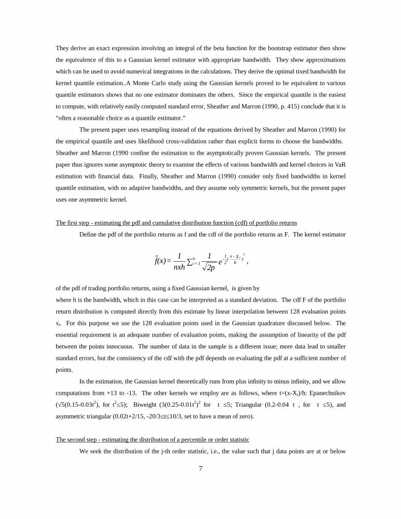
Define the pdf of the portfolio returns as f and the cdf of the portfolio returns as F. The kernel estimator

of the pdf of trading portfolio returns, using a fixed Gaussian kernel, is given by

where h is the bandwidth, which in this case can be interpreted as a standard deviation. The cdf F of the portfolio

return distribution is computed directly from this estimate by linear interpolation between 128 evaluation points

xi. For this purpose we use the 128 evaluation points used in the Gaussian quadrature discussed below. The

essential requirement is an adequate number of evaluation points, making the assumption of linearity of the pdf

between the points innocuous. The number of data in the sample is a different issue; more data lead to smaller

standard errors, but the consistency of the cdf with the pdf depends on evaluating the pdf at a sufficient number of

points.

In the estimation, the Gaussian kernel theoretically runs from plus infinity to minus infinity, and we allow

computations from +13 to -13. The other kernels we employ are as follows, where t=(x-Xi)/h: Epanechnikov

(√5(0.15-0.03t2), for t2≤5); Biweight (3(0.25-0.01t2)2 for t≤5; Triangular (0.2-0.04t, for t≤5), and

asymmetric triangular (0.02t+2/15, -20/3≤t≤10/3, set to have a mean of zero).

The second step - estimating the distribution of a percentile or order statistic

We seek the distribution of the j-th order statistic, i.e., the value such that j data points are at or below

,e21

nxh1 = (x)f )

hX - x(

21-n

1 = ii

2

π∑ˆ

8

that value and n-j above it. When the problem is stated as a percentile, p, we seek the order statistic given by

. nxp It is necessary to round the result when it is not an integer because a continuous population has continuous

percentiles, but order statistics are defined discretely (first, second,..., highest) only for a theoretical or actual

sample or a discrete population. On average, k points divide the range of a continuous random variable into k+1

intervals. Thus, the third order statistic of 99 data corresponds to the 3.00 percentile, but the third order statistic

of 100 data corresponds to the 3/101 or 2.97 percentile. In a large sample, the rounding is minor. Distributions

of percentiles require known or estimated pdfs, which we estimate, and VaR calculations as well as worst case

scenario calculations (Boudoukh, Richardson, and Whitelaw (1995)) defined over finite periods refer to order

statistics, which we analyze.

Using pdfs estimated with the kernel density estimator above, we derive the pdf of the j-th order statistic

and calculate its mean and variance. The pdf is not analytic, but its moments can be calculated by numerical

methods. The mean implied by that pdf is the estimate of VaR. From the standard error of the estimate one can

calculate confidence intervals. In this way we propose to address the problems discussed above associated with

the historical simulation approach to VaR estimation.

The distribution of the j-th order statistic is derived as follows (Stuart and Ord (1987), 445-446). Let

the order statistic be called x, with pdf gj(x) and cdf Gj(x). Then the probability that exactly j of the data are less

than or equal to x is

so that the probability that at least j of the data are less than or equal to x is

If at least j of the data are less than or equal to x, then the j-th order statistic is less than or equal to x. Thus,

equation 3 defines the cdf of the j-th order statistic. The pdf that follows from this by differentiation with respect

to x is, after some manipulation (Hoel, Port and Stone (1971), 160-163))

Equation 4 states that j-1 of the data must be less than or equal to x, one must equal x, and the rest must be greater

than or equal to x.

To obtain estimates of moments of the pdf of g from equation 4, it is necessary to integrate the pdf

,)F(x)-(1)F(xj)!-(nj!

n! j-nj

. )F(x)-(1)F(xk)!-(nk!

n! = (x)G k-nknj=kj ∑

. )F(x)-(1)f(x)F(xj)!-(n1)!-(j

n! = (x)g j-n1-jj

9

numerically. We employ Gaussian quadrature with 128 evaluation points to calculate both the mean of the

percentile, i.e., the estimate of the VaR, and the variance of the percentile, i.e., the variance of the VaR. We also

calculate the skewness and kurtosis of the estimate VaR (see Stuart and Ord (1987, p. 322)). Significant

skewness makes symmetrical confidence intervals sub-optimal, and kurtosis significantly above from 3.0

increases the width of confidence intervals beyond the width with a normal distribution.

Alternative approaches to measuring the precision of estimates

In addition to the kernel estimates, we compute two other estimates of the VaR, one based on the

empirical quantile with Monte Carlo standard errors and the other based on the assumption that the data are

normally distributed, then computing the mean and variance. For the latter purpose we employ computations

using the normal distribution.

Resampling of the data can be used to obtain an estimated standard error, although there are explicit

formulae for the variance of empirical quantiles (Sheather and Marron (1990)); we use resampling to avoid

assuming any more structure than is essential. To examine this alternative, we calculate a standard error by

employing a Monte Carlo simulation of 1,000 samples of size 100 with replacement taken from the observations.

The results of the simulation for the third percentile, the one employed in the application to financial data below,

show that the third order statistic (approximately the third percentile with a sample of size 100), is the smallest

number in the data set 81 times, the second smallest 233 times, the third smallest 279 times, and so on: fourth,

174, fifth, 111, sixth, 57, seventh, 40, eighth, 17, ninth, 5, tenth, 2, and twelfth, 1. We also determine distributions

for other percentiles which might be required in other applications. An alternative that is simpler is to impose a

parametric assumption. Here, we assume that the portfolio returns follow a normal distribution, and then the VaR

corresponding to the third percentile follows from the standard deviation of the portfolio returns. A standard error

for the percentile is calculated using a single Monte Carlo simulation rather than one for each portfolio. The

normal-based VaR is 1.88 times standard deviations of the portfolio returns below the mean. The standard error

of the normal-based estimate of VaR is calculated by multiplying the standard deviation of portfolio returns by

0.22. This multiplier is obtained from the results of a Monte Carlo simulation of 1,000 samples of size 100 with

replacement taken from a standard normal distribution. In this simulation the standard error of the estimated third

percentile was approximately 0.22 times the standard deviation of portfolio returns.

An example

To illustrate the estimation, assume that we collect three observations from an unknown distribution.

The three observations y are -5, -1, and 0. The standard deviation of this sample is 2.16. The standard bandwidth

suggested above would then be 1.56. We use 2.0 for the fixed kernel or 3.0 at the point -5 or 1.5 at the points 1

and 0. Using a fixed Gaussian kernel we evaluate the pdf at xi=-14.0, -13.9,..., 9.9, 10.0 The estimated pdf at xi

is then given by the following, where h is the bandwidth.

10

This estimated pdfs are shown in Figure 1. The value of the cdf at xi then is given by the following, in which the

evaluation is done at the same 241 points with an interval between points of 0.1.

We examine the 25th percentile, rather than the third percentile as in the next section. because, wiith

three observations, the first order statistic in the sample corresponds to the 25th percentile of the distribution.

The pdf of the 25th percentile is evaluated at the same 241 points using equation 4, substituting in equations 5

and 6.

To estimate the mean and variance of the 25th percentile or first order statistic, the pdf in equation (6) is

multiplied at each point from -14 to +10 by the value of the point or its square and summed. The Monte Carlo

quantile approach here with three points leads to drawing a random sample of size three from the sample; this

assigns weight 1/27 to 0, 7/27 to -1, and 19/27 to -5. Finally, we estimate the pdf of the first order statistic

assuming a normal distribution of y. The estimated mean and standard deviation are then -4.55836 and 2.31859

under the fixed kernel, -5.62697 and 2.88840 under the adaptive kernel, -3.82792 and 1.61607 under the

assumed normal distribution, and -3.77778 and 1.89215 under the quantile approach.

The results anticipate what the application shows. The adaptive kernel spreads the points in the left tail

more, producing an algebraically smaller (more conservative) estimate of VaR than the fixed kernel, and both are

more conservative than the normal distribution and quantile approaches.

IV. APPLICATION OF THE NEW VAR ESTIMATOR AND ALTERNATIVES

Here we examine the performance of the new estimator and two alternatives with actual trading portfolio

data from one financial institution.4 For these calculations, we assume the VaR is the third percentile of the

return distribution. Nothing about the method we propose is restrictive concerning the percentile, however; any

other could be calculated. We compare the historical simulation VaR estimate of the point determined by the

third order statistic in the sample to the VaR estimate obtained by applying the kernel estimator with various

kernels to equation (4).

Application of the new VaR estimator

The data used in the following analysis were provided by an active dealer, and they represent actual

positions of the financial institution in three trading portfolios at four dates between November 1, 1995 and

. e2h1

31

= )xf( hy - x0.53

=1kiki

2

∑π

)xf(0.1 = )xF( mi

=1mi ∑

11

February 1, 1996. These portfolios are quite diverse, containing positions in swaps, forwards, futures, options,

and cash market instruments. For each portfolio the financial institution calculated 99 or 100 simulated changes

in portfolio value based on observed changes in levels of various market risk factors, including interest rates and

exchange rates, over the 100 trading days prior to the date of the VaR calculation. For each portfolio we estimate

a single VaR using all changes in portfolio value.

Table 1 contains descriptive statistics for the sample returns of the twelve portfolios. The numbers are

re-scaled to help conceal the identity of the financial institution. The portfolio return distributions show no pattern

in skewness and are somewhat fat-tailed relative to the normal distribution (kurtosis = 3), though significantly so

for only one portfolio. Only one result is significant at the 5% level, and only one is significant at the 10% level,

exactly what would occur by chance. Those results are consistent with normality.

The results of the VaR estimation are shown in Table 2. Full results are shown for the first portfolio, and

somewhat abbreviated results are shown for the others. All kernel VaRs are more conservative when the adaptive

bandwidth is used, because it spreads the values in the lower tail of the return distribution more, resulting in more

negative values. The results for different kernels differ by as much as 20% in some cases, but the largest

differences are between the kernel VaRs and the alternative VaRs, and a number of generalizations about the

twelve sets of portfolio returns examined here are possible. All kernel VaRs are positively skewed, meaning that

they display a long upper tail. This is not problematic for risk estimation, because, while standard symmetric

confidence intervals are not optimal, they are likely to overstate the downside risk rather than understating it. No

kernel estimator displays significantly greater kurtosis than the normal.

The Epanechnikov kernel in nine of twelve cases is the most conservative. The standard errors based on

the Epanechnikov kernel are moderate, not usually the smallest or largest. This is also the easiest kernel to use

and a very popular kernel in common use. Thus, it seems to be a good choice for VaR estimation. Based on these

results, we recommend a confidence interval approach based on an adaptive Epanechnikov kernel.

The other kernel we emphasize is the Gaussian kernel. This produces the best confidence intervals,

because the VaR has insignificant skewness in only this case. However, the VaR is often, but not always, less

conservative for the Gaussian kernel, so it has statistical advantages but estimates a lower level of risk.

The biweight, triangular and asymmetric triangular kernels produce results usually more conservative

than the Gaussian results and less conservative than the Epanechnikov results, with usually higher standard errors

than either. Since they are not theoretically more valid and produce no especially interesting results, we do not

pursue them further here. All results are available from the authors.

Considering the alternatives to the kernel VaR, the normal distribution usually produces a less

conservative (algebraically higher) estimate of the VaR than the other techniques. The quantile VaR is often close

to the normal distribution VaR and somewhat algebraically higher than the others. This similarity could result

from the data being approximately normally distributed. The skewness of the quantile VaR is usually significant

but not always positive, as the kernel VaR is. The kurtosis of the quantile VaR is several times significantly less

12

than 3.0. All of these results indicate that quantile and normal VaRs result in less conservative estimates, with

potential difficulties for confidence intervals from quantiles because the skewness can be negative, with a long left

tail which is problematic for calculations of downside risk.

Figure 2 displays the estimated left tail of the distribution of returns for the first portfolio and first period

for the Epanechnikov and Gaussian kernels. This illustrates the flatter distribution estimated by the adaptive

kernel and the more bell-shaped distribution estimated by the fixed Gaussian kernel. The adaptive Epanechnikov

kernel does not estimate a unimodal distribution. Other portfolios and periods would produce similar results, as

Table 2 indicates.

The values of the fixed bandwidths selected by likelihood cross-validation are shown in Table 3 along

with the amount of probability in the region examined to find the third percentile. The Gaussian bandwidths are

noticeably small, and the Epanechnikov bandwidths are larger, but not as large as triangular bandwidths. The

differences in bandwidth are much greater than the differences in the results of using the kernels, which is typical

in kernel estimation. The probability assigned to the region examined to find the third percentile is never less

than 5.9% and for the Gaussian and Epanechnikov kernels is never less than 10.8%, another reason to use these

two in applications.

V. SUMMARY AND CONCLUSIONS

We propose a new VaR estimator that uses a kernel estimator of the density of the portfolio returns and

Gaussian quadrature to estimate the moments of any percentile or order statistic of the distribution of the returns

on a trading portfolio. This estimator is in the class of historical simulation estimators of VaR and produces a

standard error which can be used to gauge the precision of the estimated VaR. We illustrate the application of the

estimator with data from three trading portfolios of a financial institution.

Estimation using five different kernels and both fixed and adaptive bandwidths shows that the most

conservative estimates are produced by the Epanechnikov kernel, a commonly used kernel which is also relatively

easy to use (it is a quadratic function) which produces, here, moderate standard errors. The Gaussian kernel

produces the best confidence intervals, but is less conservative than the other kernels. The other three kernels

produce results usually intermediate between the results of these two. All kernels are more conservative when

adaptive estimation is used; that results from spreading more the influence in the estimation of large negative

returns. All kernels produce VaRs with positive skewness, which makes symmetric confidence intervals

problematic, because they overstate the apparent down-side risk, not because they understate it. For VaR

estimation, this is less of a problem than it would be in other statistical applications. The results here thus support

the use of Epanechnikov and Gaussian kernels with adaptive bandwidths.

We also evaluate two alternative approaches to obtaining precision information. We calculate a standard

error for the empirical quantile estimate using a Monte Carlo simulation. There is a formula for the variance of an

13

empirical quantile, but we use Monte Carlo toavoid making unnecessary assumptions in the estimation. This

approach cannot be utilized to obtain additional information about the distribution of portfolio returns, such as the

size of possible losses in the tail, while such information is produced as a by-product of the kernel approach.

Also, the skewness of the quantile VaR is sometimes negative, which causes symmetric confidence intervals to

understate the down-side risk. In the other alternative, the point estimate of VaR obtained by assuming the

portfolio return distribution is normal is usually but not always smaller than the kernel VaR and might be

unreliable for constructing confidence intervals, given the imposition of a specific distributional assumption.

Without the additional information provided by a standard error, the quality of information in the VaR

estimate is difficult to assess. The estimator proposed here permits risk managers to construct confidence

intervals to help in making ex ante risk management decisions. The estimator is also useful for evaluating the ex

post performance of the VaR estimate, because it provides information which can help explain whether large

deviations from VaR are the result of modeling problems (the more likely explanation if the standard error is

small) or market conditions (the more likely explanation if the standard error is large).

Improved information about ex-post performance may also have a significant effect on regulatory capital

charges for market risk capital applied to the largest banks. These rules set forth a capital penalty to be applied,

the severity of which depends on the number of times one day trading losses exceed the corresponding day’s VaR

estimate (Basle Committee on Banking Supervision (1996)). The relation between the number of exceptions and

the severity of the penalty is based on the assumption that the VaR is estimated without error, but supervisors of

banks may discount exceptions if they can be explained as not arising from model error. Information on the

precision of the VaR estimate may help in explaining some exceptions and assisting supervisors in decisions

concerning reductions in penalties.

14

Notes

15

References

Alexander, Carol, and C. T. Leigh. 1997. On the Covariance Matrices Used in Value at Risk Models. Journal ofDerivatives 4 (Spring), 50-62.

Basle Committee on Banking Supervision. 1996. Supervisory Framework for the use of “backtesting” inconjunction with the internal models approach to market risk capital requirements. Basle (January).

Beder, Tanya. 1995. VAR: Seductive but Dangerous. Financial Analysts Journal (September-October), 12-24.Boudoukh, Jacob, Matthew Richardson, and Robert Whitelaw. 1995. Expect the Worst. Risk 8 (September),

100-101.Boudoukh, Jacob, Matthew Richardson, and Robert Whitelaw. 1997. Investigation of a Class of Volatility

Estimates. Journal of Derivatives 4 (Spring), 63-71.Crnkovic, C. and J. Drachman. 1995. A Universal Tool to Descriminate Among Risk Measurement Techniques.

Unpublished manuscript, J. P. Morgan (September).Federal Register. 1996.”Risk-Based Capital Standards: Market Risk; Joint Final Rule. 1996.” Federal Register

61 (September 6), 47357-47378.Hendricks. Darrell. 1995. Evaluating Value-at-Risk Models Using Historical Data. Unpublished manuscript,

Federal Reserve Bank of New York (July). Hoel, Paul, Sidney Port and Charles Stone. 1971. Introduction to Probability Theory. New York: Houghton

Mifflin Company.Jackson, Patricia, David Maude and William Perraudin. 1995. Capital Requirements and Value-at-Risk Analysis.

Unpublished manuscript.Jordan, James and Robert Mackay. 1995. Assessing Value at Risk For Equity Portfolios: Implementing

Alternative Techniques. Unpublished manuscript, Virginia Tech University (July).Jorion, Phillippe. 1996. Risk2: Measuring the Risk in Value at Risk. Financial Analysts Journal 52

(November/December), 47-56. Kupiec, Paul. 1995. Techniques for Verifying the Accuracy of Risk Measurement Models, forthcoming, Journal

of Derivatives.Kupiec, Paul and James O’Brien. 1994. The Use of Bank Risk Measurement Models for Regulatory Capital

Purposes. Unpublished manuscript, Board of Governors of the Federal Reserve (March). Mahoney, James. 1995. Empirical-based Versus Model-based Approaches to Value-at-Risk. Unpublished

manuscript, Federal Reserve Bank of New York (September).Pritzker, Matthew. 1995. Evaluating Value at Risk Methodologies: Accuracy versus Computational Time.

Unpublished manuscript, Board of Governors of the Federal Reserve (November).Sheather, Simon J. and J. S. Marron. 1990. “Kernel Quantile Estimators.” Journal of the American Statistical

Association 85(410):410-416.Silverman, B.W. 1986. Density Estimation for Statistics and Data Analysis. London: Chapman and Hall.Smithson, Charles and Lyle Minton. 1996. Value-At-Risk. Risk 9 (January), 25-27.Stuart, Alan and J. Ord. 1987. Kendall’s Advanced Theory of Statistics, volume 1, fifth edition. New York:

Oxford University Press.

16

Table 1

Descriptive Statistics of the Trading Portfolios

Descriptive statistics for historical simulations of dollar returns on three trading portfolios of a financial institutionobserved at four separate dates between November 1, 1995, and February 1, 1996. The simulations consisted of 100 or99 observations each. The observations in each sample represent simulated one-day changes in the value of the portfolio. The numbers in the table have been rescaled to conceal the identity of the institution.

Portfolio & Date mean s.d. skewness s.e. kurtosis s.e. minimum maximum 1 1 -319.82 1362.34 .3550 .3325 3.5052 1.3924 -3377.63 4348.40 1 2 298.89 1253.47 -.3328 .2484 3.3251 .9872 -3304.64 3825.67 1 3 -364.94 942.77 .4617 .4216 4.6727 1.7817 -3110.00 2937.65 1 4 -274.52 1218.23 -.0090 .1432 2.1223* .3660 -2657.50 2265.03 2 1 12.65 363.24 .0878 .2129 2.8715 .7867 -956.81 973.09 2 2 2.76 115.27 -.6518** .3498 3.9302 1.3930 -370.30 268.01 2 3 8.30 79.33 -.3547 .5783 5.3064 2.6404 -306.61 236.23 2 4 7.81 125.86 -.1910 .3035 3.5088 1.2124 -383.59 361.69 3 1 -98.28 2807.31 .0104 .3676 3.8273 1.5747 -9871.10 6681.84 3 2 -495.54 2963.33 .3448 .3085 3.5103 1.2645 -7637.70 9313.66 3 3 -566.92 2143.97 .8152 .6788 6.2422 3.1269 -6590.00 8350.43 3 4 -515.09 2544.93 -.0014 .2810 3.5899 1.1252 -7952.50 6524.83

Notes:* Skewness significantly different from 0.0 or kurtosis significantly different from 3.0 at the .05 level** Skewness significantly different from 0.0 or kurtosis significantly different from 3.0 at the .10 level

17

Table 2

Results of the Estimation of VaR using Kernels and Other Methods

Kernel-Based Estimation of VaR using three different trading portfolios of a financial institution observed on fourseparate dates between November 1, 1995, and February 1, 1996

The methods:ND Normal distribution of the data assumed; normal quantiles evaluatedGK Standardized Gaussian kernel with likelihood cross-validated bandwidthGKA The preceding with adaptive bandwidthsEK Epanechnikov kernel with likelihood cross-validated bandwidthEKA The preceding with adaptive bandwidthsBK Biweight kernel with likelihood cross-validated bandwidthBKA The preceding with adaptive bandwidthsAK Asymmetric triangular kernel with likelihood cross-validated bandwidthAKA The preceding with adaptive bandwidthsTK Symmetric triangular kernel with likelihood cross-validated bandwidthTKA The preceding with adaptive bandwidthsQ Quantile estimation with bootstrap standard errors and other moments

In all cases the VaR is defined and estimated at the third percentile.

Note that all kernel results are shown for the first portfolio and first date, but for all others, only Gaussian andEpanechnikov kernel results are shown.

* Skewness significantly different from 0.0 or kurtosis significantly different from 3.0 at the .05 level** Skewness significantly different from 0.0 or kurtosis significantly different from 3.0 at the .10 level

18

Portfolio 1 Date 1

percentile: 3.00 n: 100 order statistic: 3

method mean s.d. skewness s.e. kurtosis s.e. ND -2882.10 297.25 GK -3247.23 355.16 -.0898 .2265 2.9038 .8736 GKA -3956.05 477.87 .6745* .2343 2.7617 .8278 EK -4009.36 431.01 .8683* .3634 3.5274 1.5478 EKA -4110.74 365.92 .9890* .4854 4.1238 2.3419 BK -3954.14 444.08 .9536* .4760 4.0679 2.2512 BKA -3980.28 428.97 .9844** .5110 4.2266 2.4934 AK -3941.76 441.85 .9412** .4829 4.0899 2.3028 AKA -3934.11 443.11 .9269** .4750 4.0482 2.2535 TK -3702.03 559.52 .8513* .3712 3.6707 1.5325 TKA -3711.48 557.20 .8655* .3783 3.7124 1.5703 Q -2912.45 280.50 .6276* .2506 3.0454 .9307

Portfolio 1 Date 2

percentile: 3.00 n: 100 order statistic: 3

method mean s.d. skewness s.e. kurtosis s.e. ND -2058.62 273.49 GK -2623.90 363.15 -.0852 .2285 2.9302 .8854 GKA -2945.28 455.89 .0675 .1687 2.3747 .5461 EK -3327.88 369.02 .7132* .3251 3.2727 1.3606 EKA -3429.85 325.78 .9033* .4509 3.9088 2.1421 Q -2351.85 399.23 -.8270* .2251 3.1487 .6993

Portfolio 1 Date 3

percentile: 3.00 n: 100 order statistic: 3

method mean s.d. skewness s.e. kurtosis s.e. ND -2138.09 205.70 GK -2308.14 289.62 -.2902 .2104 2.8146 .7717 GKA -2610.07 334.10 .3014 .1845 2.5184 .6205 EK -2821.44 281.01 .7581* .3485 3.4403 1.4746 EKA -2911.07 244.13 .9233* .4698 4.0118 2.2508 Q -2168.53 415.72 -.6619* .1952 2.7428 .5789

19

Portfolio 1 Date 4

percentile: 3.00 n: 99 order statistic: 3

method mean s.d. skewness s.e. kurtosis s.e. ND -2565.76 265.81 GK -2561.63 182.24 .0600 .2653 3.0718 1.1042 GKA -2963.65 378.07 -.0633 .1544 1.8408* .3081 EK -3057.55 342.93 .4710* .2216 2.4883 .7673 EKA -3124.59 306.28 .7810* .3475 3.3277 1.4706 Q -2476.46 181.81 .6661* .1655 1.8464* .3407

Portfolio 2 Date 1

percentile: 3.00 n: 100 order statistic: 3

method mean s.d. skewness s.e. kurtosis s.e. ND -670.53 79.26 GK -697.22 75.98 .0345 .2012 2.7212 .7443 GKA -754.58 80.57 .4346** .2242 2.7341 .8222 EK -744.10 92.16 .6466* .3029 3.1663 1.2313 EKA -767.96 85.47 .8561* .4141 3.7614 1.8600 Q -658.12 123.54 -1.0211* .2261 3.3302 .7120

Portfolio 2 Date 2

percentile: 3.00 n: 100 order statistic: 3

method mean s.d. skewness s.e. kurtosis s.e. ND -214.04 25.15 GK -281.87 54.68 -.2061 .1665 2.3069 .5059 GKA -299.50 61.26 -.1698 .1709 2.4906 .5615 EK -394.88 41.26 .6862* .3383 3.3021 1.4398 EKA -411.02 33.64 .8993** .4633 3.9285 2.2373 Q -272.36 66.73 -.1620 .1410 1.7318* .2105

Portfolio 2 Date 3

percentile: 3.00 n: 100 order statistic: 3

method mean s.d. skewness s.e. kurtosis s.e. ND -140.90 17.31

20

GK -130.33 13.84 .2727 .2291 2.8047 .8847 GKA -137.34 13.98 .5440* .2683 2.9626 1.0578 EK -128.39 18.75 .6177* .2779 3.0896 1.0684 EKA -131.90 18.09 .7946* .3454 3.5044 1.4028 Q -149.57 63.81 -1.2649* .2399 3.3217 .6944 Portfolio 2 Date 4

percentile: 3.00 n: 99 order statistic: 3

method mean s.d. skewness s.e. kurtosis s.e. ND -228.91 27.46 GK -279.66 44.51 -.3197 .2302 2.9101 .8717 GKA -337.01 58.55 .2235 .1716 2.3670 .5415 EK -384.80 42.74 .8253* .3733 3.5535 1.6096 EKA -398.82 35.26 .9622** .4937 4.1154 2.4107 Q -257.02 52.15 -.7029* .2353 3.5399 .8122

Portfolio 3 Date 1

percentile: 3.00 n: 100 order statistic: 3

method mean s.d. skewness s.e. kurtosis s.e. ND -5378.24 612.53 GK -5497.32 752.51 -.3857 .2486 3.0494 .9595 GKA -6937.77 836.34 .7678* .2967 3.2816 1.1478 EK -6957.16 848.50 .8719* .3788 3.6808 1.6141 EKA -7205.12 728.45 .9812* .4977 4.1929 2.4085 Q -5390.84 1697.32 -1.2419* .3045 4.3389 .9879

Portfolio 3 Date 2

percentile: 3.00 n: 100 order statistic: 3

method mean s.d. skewness s.e. kurtosis s.e. ND -6068.95 646.57 GK -6840.59 792.68 -.1246 .2220 2.8795 .8470 GKA -8170.17 1029.03 .5471* .2165 2.6304 .7474 EK -8403.99 915.03 .8298* .3557 3.4786 1.5072 EKA -8651.61 774.93 .9703* .4812 4.0911 2.3184 Q -6071.37 711.57 -.0027 .1842 3.4505 .7965

Portfolio 3 Date 3

21

percentile: 3.00 n: 99 order statistic: 3

method mean s.d. skewness s.e. kurtosis s.e. ND -4599.27 467.79 GK -4154.23 486.60 -.4807** .2639 3.2146 1.0188 GKA -4951.05 508.88 .6945* .2739 3.1768 1.0436 EK -4822.69 606.20 .7317* .3053 3.2555 1.2254 EKA -4998.76 546.75 .9123* .4353 3.9095 1.9809 Q -4429.43 1354.49 -.6849* .1383 1.6484* .1249 Portfolio 3 Date 4

percentile: 3.00 n: 99 order statistic: 3

method mean s.d. skewness s.e. kurtosis s.e. ND -5301.56 555.28 GK -6159.30 799.97 -.2173 .2276 2.9114 .8685 GKA -7091.75 1050.61 .1730 .1705 2.3465 .5369 EK -7913.77 807.68 .7819* .3497 3.4207 1.4804 EKA -8159.58 684.73 .9422* .4756 4.0325 2.2876 Q -5722.46 849.49 -.8322* .3002 4.9230** 1.1441

22

Table 3

Fixed Bandwidths and Probability Regions Examined

Fixed bandwidths estimated and percentages of the total probability distribution examined under various kernels

The kernels:GK Standardized Gaussian kernel with likelihood cross-validated bandwidthEK Epenechnikov kernel with likelihood cross-validated bandwidthBK Biweight kernel with likelihood cross-validated bandwidthAK Asymmetric triangular kernel with likelihood cross-validated bandwidthTK Symmetric triangular kernel with likelihood cross-validated bandwidth

In order to find the distribution of the third percentile, a larger proportion of the total probability distribution than .03 isexamined; the amount in each case is noted in the table below under "lower tail"

method bandwidth lower tail bandwidth lower tail bandwidth lower tail Portfolio 1 Date 1 Portfolio 2 Date 1 Portfolio 3 Date 1 GK 784.58 .2808605 177.78 .2443916 1480.87 .3506012 EK 5640.47 .1913394 1450.49 .1394316 11443.03 .1900543 BK 4317.59 .1433582 1145.66 .0997459 8910.89 .1384536 AK 2806.74 .1410123 295.84 .1970772 2567.56 .2585119 TK 5923.50 .1059986 1571.21 .0737919 12147.43 .1033329

Portfolio 1 Date 2 Portfolio 2 Date 2 Portfolio 3 Date 2 GK 630.52 .2145011 50.82 .2451256 1632.15 .3061871 EK 5028.90 .2088844 462.22 .2739407 11818.99 .2008447 BK 3944.28 .1506776 367.41 .1947175 9376.99 .1447599 AK 3615.23 .1091287 227.83 .1956062 6909.97 .1280691 TK 5364.72 .1112627 498.64 .1440354 12829.34 .1072238

Portfolio 1 Date 3 Portfolio 2 Date 3 Portfolio 3 Date 3 GK 475.34 .2556575 44.96 .2048238 930.43 .3163969 EK 3788.52 .1965846 332.09 .1077422 9054.59 .1532834 BK 2999.39 .1406272 253.66 .0795542 6960.02 .1117406 AK 2034.96 .1334085 214.58 .0629930 5621.59 .0923119 TK 4033.10 .1055919 345.08 .0593731 9415.06 .0839674 Portfolio 1 Date 4 Portfolio 2 Date 4 Portfolio 3 Date 4 GK 300.18 .1959432 67.95 .3039673 1284.50 .2572377 EK 4925.64 .1403903 504.22 .2430521 10121.26 .2221758 BK 3880.76 .1002023 396.69 .1761150 8026.40 .1593756

23

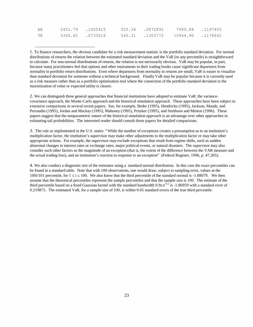
AK 2451.79 .1005415 555.34 .0872892 7085.88 .1197493 TK 5350.82 .0733018 540.31 .1303772 10944.90 .1178642

1. To finance researchers, the obvious candidate for a risk measurement statistic is the portfolio standard deviation. For normaldistributions of returns the relation between the estimated standard deviation and the VaR (or any percentile) is straightforwardto calculate. For non-normal distributions of returns, the relation is not necessarily obvious. VaR may be popular, in part,because many practitioners feel that options and other instruments in their trading books cause significant departures fromnormality in portfolio return distributions. Even where departures from normality in returns are small, VaR is easier to visualizethan standard deviation for someone without a technical background. Finally VaR may be popular because it is currently usedas a risk measure rather than as a portfolio optimization tool where the connection of the portfolio standard deviation to themaximization of value or expected utility is clearer.

2. We can distinguish three general approaches that financial institutions have adopted to estimate VaR: the variance-covariance approach, the Monte-Carlo approach and the historical simulation approach. These approaches have been subject toextensive comparisons in several recent papers. See, for example, Beder (1995), Hendricks (1995), Jackson, Maude, andPerraudin (1995), Jordan and Mackay (1995), Mahoney (1995), Pritzker (1995), and Smithson and Minton (1996). Thesepapers suggest that the nonparametric nature of the historical simulation approach is an advantage over other approaches inestimating tail probabilities. The interested reader should consult those papers for detailed comparisons.

3. The rule as implemented in the U.S. states: “While the number of exceptions creates a presumption as to an institution’smultiplication factor, the institution’s supervisor may make other adjustments to the multiplication factor or may take otherappropriate actions. For example, the supervisor may exclude exceptions that result from regime shifts, such as suddenabnormal changes in interest rates or exchange rates, major political events, or natural disasters. The supervisor may alsoconsider such other factors as the magnitude of an exception (that is, the extent of the difference between the VAR measure andthe actual trading loss), and an institution’s reaction in response to an exception” (Federal Register, 1996, p. 47,365).

4. We also conduct a diagnostic test of the estimator using a standard normal distribution. In this case the exact percentiles canbe found in a standard table. Note that with 100 observations, one would draw, subject to sampling error, values at the100i/101 percentile, for 1 ≤ i ≤ 100. We also know that the third percentile of the standard normal is -1.88079. We thenassume that the theoretical percentiles represent the sample percentiles and that the sample size is 100. The estimate of thethird percentile based on a fixed Gaussian kernel with the standard bandwidth 0.9s n-0.2 is -1.86959 with a standard error of0.219875. The estimated VaR, for a sample size of 100, is within 0.05 standard errors of the true third percentile.