estimating truck volumes on state highways: statistical approach

Estimating Truck Volumes on State Highways – A Statistical Approach

Mittal, N. Research Assistant, Dept. of Civil and Environmental Engineering, Rutgers University, New Jersey

Phone: (732) 445 3162, Fax: (732) 445 0577, E-mail: [email protected]

Golias, M.Research Assistant, Dept. of Civil and Environmental Engineering, Rutgers University, New Jersey


Boile, M.P.Assistant Professor, Dept. of Civil and Environmental Engineering, Rutgers University, New Jersey


Spasovic, L.N.Professor, School of Management, NJIT, Newark, New Jersey

Phone: (973), Fax: (973) 596-6454, E-mail: [email protected]

Ozbay, K.Associate Professor, Dept. of Civil and Environmental Engineering, Rutgers University, New Jersey

Phone: (732) 445-2792, Fax: (732) 445-0577, E-mail: [email protected]

Word Count: 4,580Figures: 1,750

Tables: 750Total word count: 7,080

Submitted for Consideration for Presentation at the 84th Annual Transportation Research Board MeetingAnd Publication in the Transportation Research Record

Submitted: August 1st, 2004Revised: November 15, 2004

TRB 2005 Annual Meeting CD-ROM Paper revised from original submittal.

Mittal, Golias, Boile, Spasovic, Ozbay 2

ABSTRACT

This paper is based on the results of a research project sponsored by the New Jersey Department of Transportation (NJDOT). It presents a statistical approach for estimating truck volumes, based primarily on classification counts and information on roadway functionality, employment, sales volume and number of establishments within the state. Models have been created that may predict truck volumes at any given location in the state highway network. Profiles of truck traffic are developed for selected roadways, indicating the Annual Average Daily Traffic, truck and passenger car volumes and percentages. The procedure has been modeled into a GIS framework, facilitating data analysis and presentation.



1) INTRODUCTION AND BACKGROUND

Knowledge of the truck volumes on local, state and interstate highways is important for highway authorities and government organizations because of their strong influence on the economy of the states and the nation overall. It has been found that shipments by truck alone account for more than half (53%) of the total tonnage, more than two-thirds (72%) of the shipments by value and nearly one quarter (24%) of the total ton-miles in the United States. (1) Estimates say that more than 375M tons of freight is transported each year in New Jersey. Trucks dominate this transportation, carrying 283M tons. The 1997 Commodity Flow Survey reported that about 67 percent of the freight tonnage that originates in New Jersey stays in the state, indicating that the truck traffic is mainly regional or local.

Trucks negatively impact the roadway network, primarily because of their massive weight, poor operating characteristics and large dimensions. These factors result in a stronger need for truck traffic estimation. Such an estimate can be helpful in pavement and bridge design and management, reconditioning and reconstruction of highway pavement, planning for freight movements, environmental impact analysis, and investment policies.

The increased importance of truck activity in both engineering and planning has created a need for truck activity estimation. Several estimation techniques have been developed using data typically available for planning applications. These techniques can provide the authorities with good statistics on the freight transportation system activity, which in turn may be used to facilitate plan development for pavement and bridge designs, prediction and planning for future freight movements, development of weight enforcement strategies, environmental impact analysis and analysis of highway investment policies.

2) LITERATURE REVIEW

Pertinent literature is briefly discussed in the following two sections, dealing with Freight Data Collectionand Freight Modeling. Freight Data Collection discusses the basic structure of state traffic monitoring programs and illustrates the different types of data collection methods that are commonly used. The Freight modeling section presents methods and tools available for freight data analysis.

2.1) Freight Data Collection

States and local highway agencies need to comply with the Highway Performance Monitoring System (HPMS) and report the traffic data collected to the Federal Government. This reporting requirement demands an efficient system with good cooperation between the different agencies and authorities.

The Traffic Monitoring Guide (2) defines the primary data collection plan as the one including: a large number of short duration counts and an appropriate number of permanent and continuously operating sites undertaking a continuous count program in the state. The classification counts at the short duration count stations are taken for a 48-hour period using the standard FHWA Highway Performance Monitoring System 13 vehicle category. Data is also collected from continuous counters to understand the variations in traffic. Weigh-In-Motion scales provide the truck and axle weight information. The collected data are then adjusted for seasonal, directional, time-of-the-day, month-of-the-year, and axle adjustments. Final data are stored in databases for future studies. Use of these data in estimating truck traffic and some related problems have been documented in the literature (3,4,5). In addition to the state program, local authorities install and operate traffic counters to collect data that may be used to complement data collected by the state.

2.2) Freight Modeling

The current state of the practice in truck trip activity estimation and freight modeling in general, falls short to today’s needs, and is at a very elementary level compared to passenger transportation modeling. Nevertheless, several techniques have been developed to estimate freight movements, which can be broadly classified under two categories, commodity-based and vehicle-based approaches.

Various states have developed their own models for modeling freight movements. The majority of these models are commodity based. The state of Virginia developed a Statewide Intermodal Freight Transportation Planning Methodology to identify problems and evaluate alternative improvements for its



transportation infrastructure. In order to have all the freight movements analyzed, commodity flows by both weight and value were considered and predictions were made for the generations and attractions of each key commodity by county and city. In the year 2000, the Indiana state authorities created a database of commodity flows within the State using the Commodity Flow Survey from the year 1997, so as to forecast the freight movement for the whole state. The state of Iowa has been active in freight transportation modeling efforts since the early 1970s, focusing primarily into the grain forecasting models. In the year 1996, the Iowa DOT developed a multi-modal and tactical model capable of modeling movements of several commodities. The Oregon DOT in 1998 initiated a study to determine the information gaps of commodity movements by truck in the state. They called the study ‘Oregon Freight Truck Commodity Flows’ study. To better estimate and forecast movement of passengers, freight and commodity into and within the state of Texas, the Texas DOT developed a Statewide Analysis Model (SAM). The models were developed to predict intra-urban area movements of freight and commodities by mode and the additional movements generated by state, regional, and national movements of freight and commodities into urban areas.

A typical vehicle-based approach develops truck trip estimates using land-use and socio-economic data (6). Based on the purpose for which a model is used, models are classified into various subgroups. These subgroups can be enlisted as; Traffic Count-Based Models, Self-Calibrating Gravity Models, Partial Matrix Techniques, GIS-based Models, Heuristic Models, Facility Forecasting Techniques etc.

The ‘Four-Step Model’ has been of the most popular techniques. (7) It is being used to predict the number of trips made within an area by type; time of day; zonal O-D pair; mode of travel used to make the trip; the routes taken etc. The release of the US DOT’s Quick Response Freight Manual (QRFM) illustrates simple techniques and transferable parameters that help in developing commercial truck movements. (8)QRFM follows a three-step process, which includes trip generation, distribution and assignment of the traffic.

Mathematical models are used to forecast freight traffic over specific network links and nodes. (9)These models are generally big in size and complexity, make numerous assumptions and require adaptations of powerful linear and non-linear programming algorithms to simplify the calculations.

This paper describes a statistical approach for estimating truck volumes on state roadways. The method is based on information and data typically collected by the states and is readily available to transportation planners. Compared to the existing methods, the new method eliminates several assumptions, avoids inconsistencies among steps of the sequential methods, and reduces the amount of data required. The trade-off is that this new method may not be used to forecast future conditions. It merely develops a picture of the current conditions on state roadways. State DOTs and Metropolitan Planning Organizations typically use their consultants for the development of freight models, analysis of current traffic conditions, and prediction of future volumes. Transportation planners in these state and regional agencies usually do not have control over the models or direct access to the tools, and rely on the results they receive by their consultants. The new method develops an easy to use tool, which can be used by transportation planners to make in-house estimates of truck volumes on state highways. These estimates are necessary in a number of key activities for a state DOT, including pavement and bridge design and management, scheduling of reconditioning and reconstruction of highway pavement, planning for freight movements, environmental impact analysis, and investment policies.

3) METHODOLOGY

The goal of this study was to create statistical models that would estimate truck volumes on the roadways of New Jersey, given the adjacent land use and socio-economic activities. A graphical representation of the methodology developed is shown in Figure 1.

The first step in the process is data collection and identification of the independent variables that would help in predicting truck traffic. Traffic counts were collected from all possible sources throughout the state. Roadway type and functionality was studied for all highways in the state and the analysis was based on the type of roadway. For the independent factors; number of employees, number of establishments and estimated sales volume (by Standard Industrial Classification, SIC) were found to be the most promising factors in predicting truck volumes. Regression models were built and truck volume predictions were made for the locations where no prior information was available. Profiles with truck volumes and percentages were created to better understand the traffic conditions. Finally, the procedure was implemented into a GIS framework to facilitate data visualization and understanding.



Figure 1 here

3.1) DATA COLLECTION

The data collection effort for the project was divided into two areas: traffic counts with truck classification data used as the dependent variables, and socio-economic activity as the explanatory variables. Every state has a traffic data collection program, through which traffic counts are taken at certain locations throughout the state. In New Jersey, as is the case in most of the other states, a limited number of locations are surveyed each year due to budgetary constraints. The NJDOT Bureau of Data Development uses a set of criteria for the selection of the count locations, including good geographic, temporal and spatial coverage of the traffic. Typical vehicle – based models develop truck trip estimates using land use and socioeconomic data. These explanatory variables are not necessarily sufficient to explain truck traffic data. Nevertheless, and according to the NCHRP Synthesis 298 (2001), these are typically the variables being used.

Dependent Data

The majority of the traffic counts were obtained through the NJDOT’s Bureau of Data Development. These counts consist of both long and short duration counts. Short duration counts were adjusted for axle correction and pattern factors. A number of supplemental traffic counts from toll authorities such as the New Jersey Turnpike Authority and the Delaware River Joint Bridge Commission were considered as well. Due to the different classification scheme that was used for these counts, they were not used in the project. In all, a dataset consisting of 270 locations as shown in Figure 2 was created for the analysis. The dataset includes all the NJDOT classification counts that were collected for the year 2000.

Figure 2 here

Independent Variable Dataset

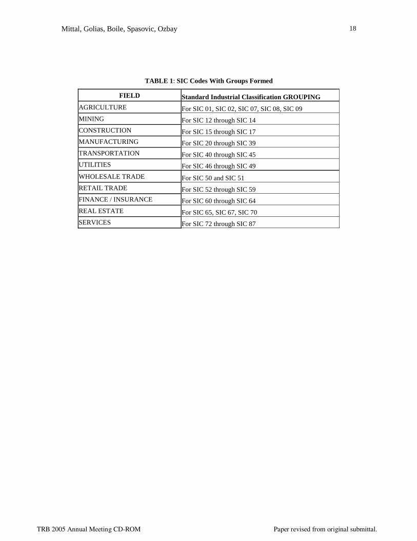
The data for the independent variable dataset includes number of employees, sales volume, and number of establishments. It has been extracted from the ESRI BIS data (Environmental Systems Research Institute Business Information Solutions), a comprehensive list of businesses licensed from InfoUSA. The database used includes employment, sales volume and number of establishments in NJ for year 2001. Data items included business name and location, franchise code, industrial classification code, number of employees, and sales volume. Information on the number of employees, sales volumes and number of establishments under each of the SIC codes included in the database was extracted. For the purpose of this analysis, SICs were grouped as shown below in Table 1.

Table 1 here

The independent data were extracted in the shape of bands (or “buffers” in the GIS parlance) along the highway sections that were defined. Uniform sections of highway were defined based on major intersections or cross roads and change in roadway functionality. Circular buffer areas were also considered, however, due to the limited number of counting locations and problems with occasional double counting and overlapping, it was found that a band shaped buffer worked best and gave more uniform estimates.

Roadway Information

Based on the area they serve, network continuity and traffic characteristics, roadways are classified into various categories. Table 2 shows the roadway classification based on functional and administrative characteristics.

Table 2 here



3.2) STATISTICAL ANALYSIS

Using the above described data; relationships between truck volumes and adjacent activities were built. Sensitivity analysis was performed to determine the change in the models’ behavior with a change in the band’s width. The best model for each roadway class was selected based on the bandwidth that produced the best results.

Stepwise linear regression was used to create the predictive models. This method selects the most significant variables to be used into the model and removes the non-significant variables, thus finally building the model that would best fit the data.

Based on the functional classes of the roadways and performing some preliminary analysis such as clustering, the following roadway grouping was developed:

FC 1,2 = rural interstate and major arterials FC 6, 7, 8, 9 = rural minor arterials, collectors, and localFC 11 = urban interstateFC 12 = urban expressways and parkwaysFC 14 = urban major arterials FC 16, 17, 19 = urban minor arterials, collectors, and local

Models were developed for tucks (FHWA Highway Performance Monitoring System vehicle class 6 through class 13), as agreed upon during a meeting with NJDOT officials. Vehicle class 5 was taken out of the analysis because of the arguable way that class 5 vehicles are classified. Depending on the data collection system used, very often cars and small pick-up trucks and vans are classified as class 5 trucks.

Model Analysis

The statistical software package SAS was used to perform the regression analysis and build the models for truck volume prediction. R-square values were used to determine the model’s predicting capability.

Sensitivity Analysis

Sensitivity analysis was performed to determine how “sensitive” a model is with respect to the size of the activity area considered in the analysis. Buffers considered varied with widths of 0.25, 0.5, 0.75, 1.0, 1.25, 1.5, 2.0, 3.0, and 5.0-mile. The resulting R-square values of the models are shown in Figure 3.

Figure 3 here

The figure shows that the models are sensitive to the area considered in the analysis. A general trend is that for lower level roads a small buffer area seems to work better, whereas for higher-level roads (interstates, expressways) a larger radius performs better. A very large radius negatively affects the models, a result that is expected, since activity in such a large area generates traffic that is distributed over several roadways and is not necessarily part of the traffic in the specific roadway segment under consideration.

Final Models Built

Based on the approach and methodology presented in the previous section, the following models were built. The independent variables that enter the model are all found to be significant at alpha value = 0.15.

1. Trucks on Rural InterstateY = 412.07 + 22.54 (emp_transp) +27.83 (emp_real) + 0.011 (sales_agri) + 0.006 (sales_whol) + 0.172 (sales_fin) –70.67 (cnt_const) + 341.59 (cnt_manu) – 393.34 (cnt_transp) – 469.29 (cnt_fin)

2. Trucks on Rural MinorY = 64.445 + 0.726 (emp_const) – 0.265 (emp_serv) + 13.27 (cnt_manu) + 17.43 (cnt_whol)

3. Trucks on Urban Interstates



Y = 9998.6 – 98.36 (emp_agri) + 108.36 (emp_const) – 21.29 (emp_util) + 6.489 (emp_fin) + 0.957 (emp_serv) – 0.59 (sales_const) + 0.007 (sales_manu) – 0.037 (sales_fin) + 204.20 (cnt_whol)

4. Trucks on ExpresswaysY = 4889.5 + 126.27(emp_agri) – 500.03(emp_min) – 1.55 (emp_fin) + 1.15 (emp_serv) + 0.31 (sales_agri) + 1.34(sales_min) + 0.36 (sales_util) – 0.015 (sales_reta) – 270.66 (cnt_agri) + 977.55(cnt_util) + 322.21(cnt_trans) –119.01 (cnt_whol) –46.37 (cnt_serv)

5. Trucks on Urban MajorY = 1501.3 + 3.397 (emp_whol) – 53.17 (cnt_fin)

6. Trucks on Urban MinorY = 119.43 + 0.77 (emp_transp) – 0.385(emp_reta) + 0.003 (sales_reta) – 30.14(cnt_agri) + 818.83 (cnt_mini) + 13.72 (cnt_ fin) + 4.664 (cnt_real)

Table 3 shows the standard error associated with each model.

Table 3 here

The above analysis shows that the models that have been estimated for higher-level facilities, such as interstates and expressways, have a substantially higher intercept value compared to those for lower level facilities. The higher intercept accounts for the through traffic on these roadways, meaning traffic that does not have its origin and/or destination in the state but uses state roadways to move between points of origin and destination. Thus, the models implicitly account for this ‘overhead truck traffic’. Estimates of through traffic on major highways were not available at the time of the project. If such estimates become available in the future, the value of through traffic could be subtracted from the corresponding observed counts in their respective highway locations, and the procedure described above would be used to develop models to estimate locally generated traffic on higher-level roadway sections. Typically, lower level facilities do not carry large volumes of through traffic, thus inclusion of through truck volume estimates would not affect these models.

Truck Traffic Profile

After the models were created and predictions were made for the locations where no prior information was available on trucks, traffic profiles were produced. To present an example of the traffic profiles created, Interstate 78 in New Jersey is selected and its observed and predicted truck volumes are shown in figure 4. Interstate 78 was selected because it is one of the roadways analyzed in this work with the highest number of observed counts. Figure 5 shows the observed and estimated truck traffic percentage on I-78. It can be observed that the estimations provided by the models presented in this paper are fairly close to the actual observed counts. Similar observations were made in all roadways considered in the analysis. Overall, the models seem to make reasonable estimates of the truck volumes. It is expected that a larger number of observations would help train better models and increase their accuracy in estimating truck volumes.

Figure 4 and 5 here

These profiles help in better visualizing and understanding the flow of truck traffic throughout New Jersey and validate the models for the sections with observed data.

GIS based Interactive Tool

The truck volume estimation models were implemented within GIS, to facilitate calibration and data visualization. The classification count and econometric data were also included in the GIS platform. The resulting tool allows the user to select a roadway segment and, depending on its functional grouping, use the appropriate model to estimate truck volumes and truck percentages. Graphical images showing the traffic profile on the selected segment and the adjacent ones are generated. A snapshot of the GIS-based tool is shown in Figure 6



Figure 6 here

4) COMPARISON WITH THE QRFM AND THE NJ STATEWIDE MODEL

The Quick Response Freight Manual (QRFM) or three-step approach for modeling truck traffic was compared with the regression approach presented in this paper. The two approaches are similar in that they predict truck traffic based on adjacent economic and land-use activity, and categorize employment data by SIC. A major point of distinction between the two approaches was that regression did not make as many assumptions as the QRFM approach and avoided inconsistencies that are typical among the steps of sequential processes such as QRFM. Regression is thus found to be closer to the real world situation and more practical in its application.

Predictions were made using the regression models and the predicted truck volumes were compared with those from the existing statewide truck model for New Jersey, which is based on a QRFM-like approach. Regression and statewide truck model results are plotted in GIS along with the observed truck volumes (from the vehicle classification counts). Comparison of the results shows that the regression approach made, in general, better estimates (closer to the observed counts) than the statewide model. Figure 7 below shows a snapshot of Interstate 78 in New Jersey with observed truck volumes and predicted volumes from both regression and the statewide truck model. The bottom part of the figure shows a zoomed-in image of the same interstate.

Figure 7 here

5) RESULTS AND CONCLUSIONS

The following conclusions were drawn based on the results of this study:• Building models considering roadway classes is significant, as different roadways attract different

types of truck traffic and truck volumes.• Number of Employees, Estimated Sales Volume and the Number of Establishments based on the

Standard Industrial Classification for the region are considered to be good predictors of truck volumes.• Creating vehicle profiles for different roadway sections helps in understanding the traffic flow patterns

within the state• Models become sensitive to the area considered along the section. A larger bandwidth resulted in better

truck volume estimates for roadways such as Interstates and Expressways. Models for minor roads gave better estimates when smaller buffer areas were considered.

• Although preliminary results obtained through this study are promising in terms of the proposed methodology and results, it is recognized that a much larger set of counts should be considered in order to obtain more sound statistical models and more accurate results. Additional data and surveys (example: cordon counts or license plate surveys) should be carried-out in order to provide accurate estimates of the ‘through traffic’ on the various major highways.

• The proposed method is not intended to “replace” or “compete” with existing methods and may not be used as a freight-forecasting tool. It can effectively be used for facility planning, corridor planning, and strategic planning for transportation systems including pavement and bridge design and management, reconditioning and reconstruction of highway pavement, planning for freight movements, environmental impact analysis, and investment policy applications.

• This tool can help planners in obtaining truck volume, flow and percentage estimates on state roadways without having to use freight forecasting tools which require more data, time, and resources. This kind of analysis is typically outsourced to consultants by state DOTs. Having the proposed tool available in-house, estimates on truck volumes can easily be made. Any additional information on future scenarios and what-if kind of analysis will have to use the traditional channels.

ACKNOWLEDGMENTThis research has been supported by the New Jersey Department of Transportation, the Center for Advanced Infrastructure and Transportation and the National Center for Transportation and Industrial Productivity. This support is gratefully acknowledged, but implies no endorsement of the conclusions by NJDOT, CAIT and NCTIP. The contents of this paper reflect the views of the authors who are responsible for the facts and the accuracy of the information presented herein.



7) REFERENCES

1. Boile M.P., “Estimation of Truck Volumes and Flows,” A Project Report by the Center For Advanced Infrastructure and Transportation (CAIT), Rutgers University, June 2001

2. “Traffic Monitoring Guide,” U.S. Department of Transportation, Federal Highway Administration, Office of Highway policy Information, May 2001

3. Sharma S.S. , Liu G. X. , Thomas S. , “Sources of Error in Estimating Truck Traffic from Automatic Vehicle Classification Data”, Journal of Transportation and Statistics, October 1998, p. 89-93,

4. Weinblatt H. , “Using Seasonal and Day-of-Week Factoring to Improve Estimates of Truck Vehicle Miles Traveled,” Transportation Research Record 1522, p. 1-8

5. Mingo, R.D., and Wolff, H.K. Improving National Travel Estimates for Combination Vehicles. In Transportation Research Record 1511, TRB, National Research Council, Washington, D.C., 1995, pp 42-46

6. Boile, M.P., Benson S. and Rowinski J. “Freight Flow Forecasting - An Application to New Jersey Highways.” Journal of the Transportation Research Forum, Vol. 39, No. 2, 2000 pp. 159-170

7. Meyer, Michael and Eric Miller. Urban Transportation Planning, Second edition. McGraw-Hill, 20018. Marker J.T. Jr., and Goulias K.G., “Truck Traffic Prediction Using Quick Response Freight Model

Under Different Degrees of Geographic Resolution, Transportation Research Record 1625, 1998, p. 118-123

9. Friesz T.L., “Strategic Freight Network Planning Models,” Handbook of Transportation Modeling, 2000, p. 527-537



LIST OF FIGURES

FIGURE 1: Methodology ..............................................................................................................................11FIGURE 2: Classification Count Sites ..........................................................................................................12FIGURE 3: Sensitivity Analysis....................................................................................................................13FIGURE 4: Traffic Profile With Observed And Predicted Truck Traffic On Interstate-78 ..........................14FIGURE 5: Traffic Profile With Observed And Predicted Truck Percentage On Interstate-78....................15FIGURE 6: GIS Based Modeling Tool Application......................................................................................16FIGURE 7: Sections On I-78 With Observed And Estimated Truck Volumes.............................................17

LIST OF TABLES

TABLE 1: SIC Codes With Groups Formed .................................................................................................18TABLE 2: Roadway Classification ...............................................................................................................19TABLE 3: Standard Errors Associated With Each Model ............................................................................20



FIGURE 1: Methodology

DATA COLLECTION: TRUCK VOLUMES

CREATION OF SECTIONS ALONG THE OBSERVATIONS

TAKE INDEPENDENT DATASET IN BANDS OF 0.25, 0.5, 0.75, 1.0, 1.5, 2.0, 3.0 AND 5.0 MILES

BUILD MODELSY = a + b1x1 + b2X2 + …+ bnXn

SENSITIVITY ANALYSIS

PREDICT TRUCK VOLUME ON SECTIONSWHERE NO COUNTS ARE TAKEN

CREATE TRAFFIC PROFILES ON SELECTED ROADWAY SECTIONS

MODEL THE PROCEDURE INTO A GIS BASED PLATFORM

RESULTS / CONCLUSIONS



FIGURE 2: Classification Count Sites



Model Sensitivity by Buffer Widths

0

0.2

0.4

0.6

0.8

1

1.2

Rural Interstate Rural Minor Urban Interstate Expressways Urban Major Urban Minor

R-s

quar

e

0.25

0.5

0.75

1

1.25

1.5

2

3

5

FIGURE 3: Sensitivity Analysis



FIGURE 4: Traffic Profile With Observed And Predicted Truck Traffic On Interstate-78



FIGURE 5: Traffic Profile With Observed And Predicted Truck Percentage On Interstate-78



FIGURE 6: GIS Based Modeling Tool Application



FIGURE 7: Sections On I-78 With Observed And Estimated Truck Volumes



TABLE 1: SIC Codes With Groups Formed

FIELD Standard Industrial Classification GROUPING

AGRICULTURE For SIC 01, SIC 02, SIC 07, SIC 08, SIC 09

MINING For SIC 12 through SIC 14

CONSTRUCTION For SIC 15 through SIC 17

MANUFACTURING For SIC 20 through SIC 39

TRANSPORTATION For SIC 40 through SIC 45

UTILITIES For SIC 46 through SIC 49

WHOLESALE TRADE For SIC 50 and SIC 51

RETAIL TRADE For SIC 52 through SIC 59

FINANCE / INSURANCE For SIC 60 through SIC 64

REAL ESTATE For SIC 65, SIC 67, SIC 70

SERVICES For SIC 72 through SIC 87



TABLE 2: Roadway Classification

Roadway Classification Name1 Rural Interstates2 Rural Other Principal Arterials6 Rural Minor Arterials7 Rural Major Collectors8 Rural Minor Collectors9 Rural Local

11 Urban Interstates12 Urban Other Freeways and Expressways14 Urban Other Principal Arterials16 Urban Minor Arterials17 Urban Collectors19 Urban Locals



TABLE 3: Standard Errors Associated With Each Model

Rural Interstate

VariableParameter Estimate

Standard Error

Intercept 412.07 161.82EMP_TRANSP 22.54 2.65EMP_REAL_E 27.83 2.30SALES_AGRI 0.01 0.00SALES_WHOL 0.01 0.00SALES_FINA 0.17 0.02COUNT_CONS -70.67 13.56COUNT_MANU 341.60 52.83COUNT_TRAN -393.35 58.35COUNT_FINA -469.29 41.34Rural Minor


Standard Error

Intercept 64.45 17.57EMP_CONSTR 0.73 0.36EMP_SERVIC -0.27 0.05COUNT_MANU 13.27 6.14COUNT_WHOL 17.42 4.44Urban Interstate


Standard Error

Intercept 9998.65 134.05EMP_AGRICU -98.36 16.96EMP_CONSTR 108.46 14.25EMP_UTILIT -21.30 2.74EMP_FINANC 6.49 1.46EMP_SERVIC 0.96 0.55SALES_CONS -0.59 0.08SALES_MANU 0.01 0.00SALES_FINA -0.04 0.01COUNT_WHOL 204.20 41.62



Expressways


Standard Error

Intercept 4889.51 148.91EMP_AGRICU 126.27 5.95EMP_MINING -500.04 37.83EMP_FINANC -1.55 0.57EMP_SERVIC 1.15 0.17SALES_AGRI 0.31 0.01SALES_MINI 1.34 0.17SALES_UTIL -0.37 0.00SALES_RETA -0.01 0.00COUNT_AGRI -270.66 16.52COUNT_UTIL 977.55 11.29COUNT_TRAN 322.21 6.89COUNT_WHOL -119.02 3.72COUNT_SERV -46.37 1.81Urban Major


Standard Error

Intercept 1501.30 507.80EMP_WHOLES 3.40 1.22COUNT_FINA -53.17 36.42Urban Minor


Standard Error

Intercept 119.44 16.99EMP_TRANSP 0.78 0.15EMP_RETAIL -0.39 0.26SALES_RETA 0.00 0.00COUNT_AGRI -30.14 8.96COUNT_MINI 818.83 149.27COUNT_FINA 13.72 5.78COUNT_REAL 4.66 2.45COUNT_SERV -2.00 0.53


estimating truck volumes on state highways: statistical approach

Documents