1

Estimating the Medium-term Effects of

the ASEAN Economic Community*

Hiro Lee†

Osaka University

Michael G. Plummer

OECD and Johns Hopkins University, SAIS-Bologna

April 2010

Abstract

Consequences of the ASEAN Economic Community (AEC) are investigated using a dynamic computable general equilibrium (CGE) model. Quantitative assessments of the effects on economic welfare, trade flows and sectoral output are offered. When the removal of trade barriers are combined with reductions in administrative and technical barriers and lowering the trade and transport margins under the assumption of endogenously determined productivity, the estimated welfare gains for the year 2015 range from 1.1% in Indonesia to 9.4% in Thailand. The results suggest that streamlining customs procedures and other reductions in administrative and technical barriers, as well as increased competition and improvements in infrastructure, are significant in enlarging the benefits of the AEC. JEL classification: F15, F17 Keywords: ASEAN, AEC, CGE model

* The authors are grateful to Mordechai E. Kreinin and Dominique van der Mensbrugghe for their helpful comments. † Corresponding author. Osaka School of International Public Policy, Osaka University, 1-31 Machi-kaneyama-cho, Toyonaka, Osaka 560-0043, Japan. Email: hlee@osipp.osaka-u.ac.jp

2

1. Introduction

Founded in 1967 with the Bangkok Declaration, the Association of Southeast Asian

Nations (ASEAN) is the most advanced institution of regional cooperation in Asia and one

of the oldest. At first, its goals were mainly political in nature. In particular, it sought to

promote peace in what was at that time a volatile region. ASEAN did not attempt any

significant economic cooperation initiatives until the new international political environ-

ment emerged at the end of the 1980s. Its first major initiative was ASEAN Free Trade

Area (AFTA), which was established in 1992 and originally only covered trade in

manufactured goods to be liberalized over a 15-year period.1 However, ASEAN subse-

quently broadened the scope and shortened the implementation period of AFTA so that it

was technically in full effect at the beginning of 2004 for the original ASEAN countries2

At the 2002 ASEAN Summit in Phnom Penh, it was proposed that the region

should consider the possibility of creating an ASEAN Economic Community (AEC) by

2020. In the 2007 “Cebu Declaration” the ASEAN leaders not only formalized this

commitment but actually pushed up the deadline to 2015. The action plan for the

implementation of the AEC was published in the form of the “ASEAN Blueprint” in

November 2007. As part of the AEC process, ASEAN developed the ASEAN Charter,

which was ratified by each ASEAN member state and went into effect in December 2008.

Specifically, the AEC has the following four goals:

and Brunei Darussalam (“ASEAN-6”), although there are transitional periods for products

on the temporary exclusion lists, including some agricultural and food products and

automobiles.

1. A single market and production base, characterized by a free flow of goods, services, investment and skilled labor, as well as a freer flow of capital.

2. A competitive economic region, characterized by sound competition policy, con-sumer protection, intellectual property rights protection, infrastructure development, sectoral competition in energy and mining, rationalized taxation and e-commerce.

1 Liberalization was somewhat loosely defined, as it left tariffs in the 0–5% range rather than the traditional 0%. 2 Indonesia, Malaysia, the Philippines, Singapore and Thailand.

3

3. Equitable economic development, characterized by small and medium enterprise development and enhancement of initiatives geared to help the least-developed ASEAN member states.

4. Integration into the global economy, with ASEAN centrality and participation in global supply networks.

In sum, the primary goal of economic integration in ASEAN, as articulated by its

leaders, is to reduce transactions costs associated with economic interchange and to make

the region more attractive to multinational corporations wishing to take advantage of its

diversity and openness in rationalizing production networks. In this sense, it is both

determining and determined by the new wave of outward-oriented regionalism in Asia.

The objective of this paper is to evaluate the potential effects of the AEC on

economic welfare, trade flows and sectoral output of the member states using a dynamic

computable general equilibrium (CGE) model. The model incorporates endogenously

determined sectoral productivity and reductions in transactions costs, including the trade

and transport margins and frictional trade costs (i.e. trade-related risks and administrative

and technical barriers to trade). The next section gives an overview of the model. Section 3

provides a brief description of the baseline and policy scenarios, followed by assessments

of computational results in section 4. The final section offers conclusions and possible

extensions of the paper.

2. Overview of the CGE Modeling Framework

The model used in this study is a modified version of the LINKAGE model

developed by van der Mensbrugghe (2005). This model has been extensively used for the

comparative analysis of alternative trade integration scenarios, including an assessment of

various Doha Round proposals by Anderson et al. (2006) and the evaluation of various

free-trade agreement scenarios in East Asia by Lee and van der Mensbrugghe (2008). In

many respects the structure of the LINKAGE model is similar to two other widely used and

cited global trade models, specifically, the Purdue-based GTAP, as elaborated in Hertel

4

(1997) and MIRAGE, sponsored by CEPII in Paris and discussed by Bchir et al. (2002).3

The core of all three frameworks is a comparative static CGE model, although all three

incorporate specific variations. For example, LINKAGE and MIRAGE are typically used for

undertaking a recursive dynamic analysis, where specific assumptions regarding popula-

tion and labor growth, capital accumulation and productivity are invoked in order to

develop a baseline scenario from which different policy shocks are then examined.4

The LINKAGE model entails a standard CGE paradigm, built around the circular

flow of the economy, where on the supply side, goods and services are produced by

combining intermediate inputs and factors (e.g., labor, capital and land). A nested constant

elasticity of substitution (CES) structure captures the substitution and complementary

effects across intermediate goods and factors. In most sectors, the degree of substitution

between capital and labor constitutes the core relation, while intermediate goods are taken

to be a fixed proportion of output.

5

An open-economy CGE model entails a somewhat more complicated structure,

since domestic production needs to be allocated between domestic and multiple foreign

A second node of the circular flow, relating to

economic agents’ supply of the needed factors of production and their factor earnings, is

specified in the LINKAGE framework by a single representative household that receives all

factor income. Finally, a third node, characterizing agents’ demand for final goods and

services, uses the extended linear expenditure system (ELES) whereby purchases of goods

and services are simultaneously determined with savings (Lluch, 1973). As in the

conventional CGE model, such as those developed by Dervis et al. (1982) and Löfgren et

al. (2002), constant returns to scale and perfect competition are assumed in the goods and

services market, and product and factor prices are determined by equilibrium in their

respective markets.

3 van der Mensbrugghe (2006) offers a discussion of representative numerical results based on the LINKAGE model, along with a summary comparison to those using GTAP. 4 Although a dynamic version of GTAP has been developed by Ianchovichina and McDougall (2000), a majority of GTAP applications involve a static version of that model. 5 One strength of the LINKAGE model is a rather detailed formulation for agricultural production, in which land use plays a key role, as, for example, in the choice between intensive versus extensive crop production, or range-fed, as compared to other smaller livestock undertakings. The energy sector also constitutes a separate activity, which is assumed to be a near-complement to capital in the short run, but a substitute for capital in the long run.

5

markets, while domestic demand can be met by goods produced either domestically or

from abroad. In this regard, the standard LINKAGE model assumes that domestic output is

supplied homogeneously from all markets, with the law of one price holding, so that

producers can switch their sales across market destinations costlessly.6 On the demand

side, products are differentiated for both producers and final consumers on the basis of

their origin, in keeping with the so-called Armington assumption.7

The model distinguishes between four interrelated price categories for traded

goods, which entail four separate instruments. The initial price producers receive for their

exported goods is designated as PE, while the FOB price, denoted as WPE, reflects

domestic export taxes or subsidies. The CIF price, WPM, includes the trade and transport

margins, represented by the ad valorem wedge ζ, as well as frictional trade costs,

corresponding to an iceberg parameter λ.

More specifically, the

LINKAGE framework relies on a nested CES structure, where at the top nested level, each

agent chooses to allocate aggregate demand between locally produced goods and an

aggregate import bundle, while minimizing the overall cost of the aggregate demand

bundle. At the second level, aggregate import demand is allocated across different trading

partners, again using a CES specification, wherein the aggregate costs of imports are

minimized. This open-economy formulation generates a much broader set of market

equilibria, whereby the supply and demand for each traded good is required to be equal.

Hence, if the closed economy model had n equilibria for n goods, the global model has

r x n equilibria for domestic goods and r x r x n equilibria for traded goods, where r is the

number of modeled countries/regions.

8

6 The model also allows for a finite constant elasticity of transformation (CET) function, which applies across market destinations, and uses a two-level nested CET specification. At the top nested level, production is allocated between the domestic market and aggregate exports, so as to maximize revenue. At the second level, a CET function is used to allocate aggregate exports across foreign markets, while maximizing total export revenue.

Thus, the relationship between the FOB and CIF

prices is given by

7 See Armington (1969). 8 Such an iceberg specification for transportation costs was formulated by Samuelson (1952), based on a concept developed earlier by von Thünen.

6

( ) irrirrirrirr WPEWPM ,',,',,',,', 1 λζ+= (1)

for the different r and r' combinations of exporting and importing regions/countries and i

commodities. Finally, the domestic price of imports, PM, equals the CIF price, WPM, plus

tariffs and/or the tariff-equivalent effects of a range of possible commercial policies. In the

subsequent analysis, an increase in irr ,',λ corresponds to a reduction in trade-related risks,

lower administrative barriers to trade (e.g., customs procedures), and/or a fall in technical

barriers (e.g., mutual recognition of product standards). In sum, trade facilitating policy

initiatives imply an increase in the value of irr ,',λ .

Final demand in the model is split into three categories, involving a representative

household, the public sector and the investment account. Public expenditure is specified as

fixed as a share of GDP and investment is determined by the total savings of the economy,

thereby leading to a different pattern of demand expenditures relative to that of households.

There are three closure rules relating to final goods expenditures in each country. First, the

government deficit is assumed to be fixed, while a lump sum tax borne by the

representative household is endogenously determined, so as to meet the public deficit

target. Thus, trade reform can generate an increase in the direct taxation of consumers, as a

result of reduced tariff revenues. Second, investment equals the sum of private, public and

foreign savings. Third, the level of foreign saving is fixed; i.e., the current account balance

is taken as exogenously given. The latter implies that an ex ante change in import demand

generates an offsetting adjustment in the real exchange rate.

The model was calibrated to a 2004 base year using version 7 of the GTAP

database.9

9 A detailed description of version 7 of the GTAP database is offered by Narayanan and Walmsley (2008).

Although the LINKAGE model can be analyzed for 113 countries/regions and 57

sectors, this more detailed database has been aggregated in the current analysis, and relates

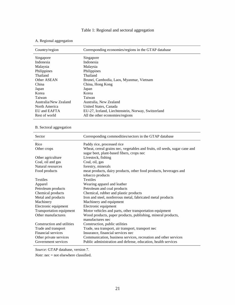
to 14 countries/regions and 20 sectors as shown in Table 1. More specifically, the

country/region breakdown includes five individual ASEAN economies (Singapore,

Indonesia, Malaysia, the Philippines and Thailand), an aggregation of other ASEAN

economies (Brunei, Cambodia, Laos, Myanmar and Vietnam), four East Asian economies

7

(China, Japan, Korea and Taiwan), as well as regional country groupings for

Australia/New Zealand, North America, Europe (EU and EAFTA) and the rest of the

world. The values of key parameters, such as demand, supply and substitution elasticities,

are based upon the previous empirical estimates. The model calibration primarily consists

of calculating share and shift parameters to fit the model specifications to the observed

data, so as to be able to reproduce a solution for the base year.10

The Appendix provides

the values of the key elasticities used in the model.

3. The Baseline and Policy Scenarios

3.1 The Baseline Scenario

In order to evaluate the effects of the ASEAN Economic Community, the baseline

scenario is first established, showing the path of each of the 14 economies/regions in the

absence of ASEAN economic integration over the period 2004-2020. Population and labor

force growth are assumed exogenous, in line with assumptions made by the UN, such that

the growth of the labor force growth equals the growth of the working age population (ages

15-64). Real GDP growth rates are also exogenous in the baseline in order to be consistent

with the actual growth rates for 2004-2008 and the World Bank’s growth forecast for

2009-2020. The basic capital accumulation function equates the current capital stock to the

depreciated stock inherited from the previous period plus gross investment. In the baseline

the trade and transport margins are assumed to decline by 1 percent per annum in every

country/region, which is consistent with the recent trends.

Sectoral productivity is determined by three components: a uniform economy-wide

factor that is calibrated to achieve the given GDP target, a sector-specific factor related to

the degree of openness, and a shift term that permits constant deviations across sectors

beyond the differences in openness. More specifically, the sector-specific factor intended

to capture the sensitivity of changes in productivity to an economy’s openness, χi,t

10 Some of the calibrated parameters are adjusted in the dynamic scenario, as explained by van der Mensbrugghe (2006).

, is

given by the formula:

8

i

ti

tititi X

Eη

φχ

=

,

,,, (2)

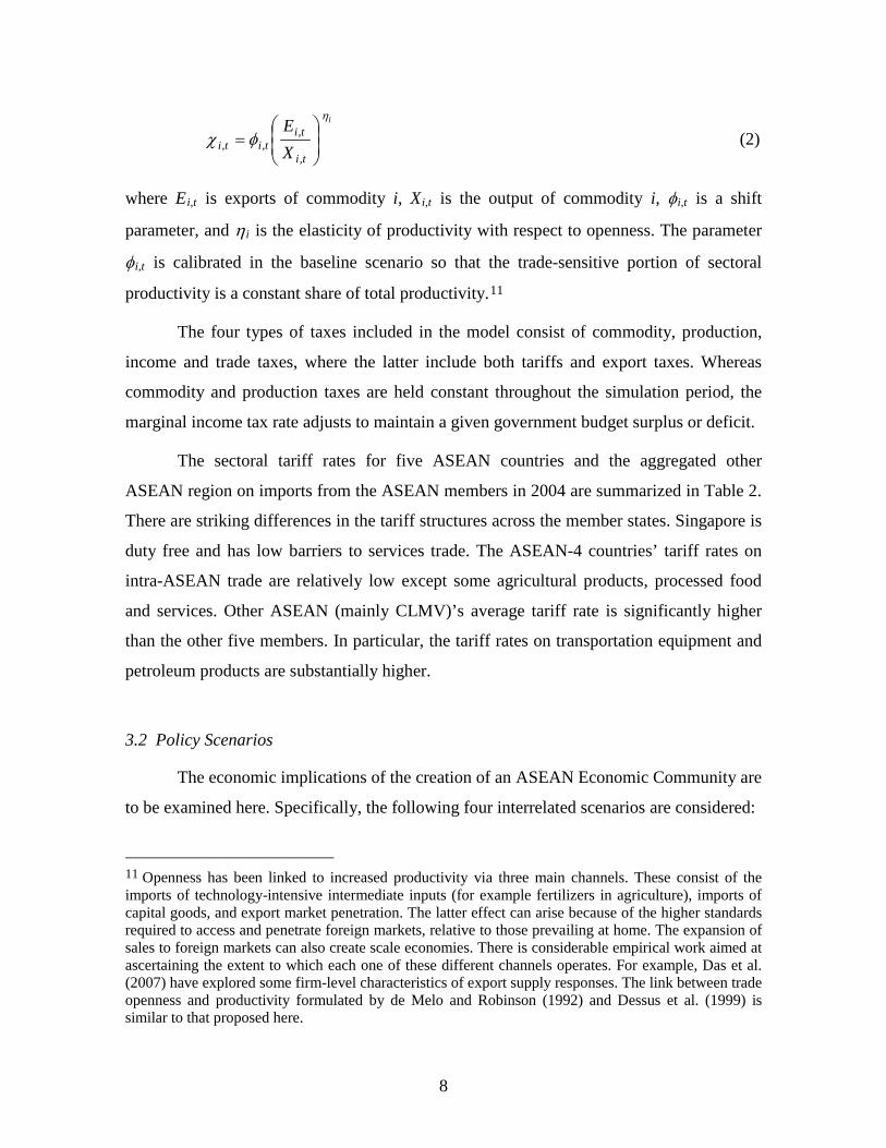
where Ei,t is exports of commodity i, Xi,t is the output of commodity i, φi,t is a shift

parameter, and ηi is the elasticity of productivity with respect to openness. The parameter

φi,t is calibrated in the baseline scenario so that the trade-sensitive portion of sectoral

productivity is a constant share of total productivity.11

The four types of taxes included in the model consist of commodity, production,

income and trade taxes, where the latter include both tariffs and export taxes. Whereas

commodity and production taxes are held constant throughout the simulation period, the

marginal income tax rate adjusts to maintain a given government budget surplus or deficit.

The sectoral tariff rates for five ASEAN countries and the aggregated other

ASEAN region on imports from the ASEAN members in 2004 are summarized in Table 2.

There are striking differences in the tariff structures across the member states. Singapore is

duty free and has low barriers to services trade. The ASEAN-4 countries’ tariff rates on

intra-ASEAN trade are relatively low except some agricultural products, processed food

and services. Other ASEAN (mainly CLMV)’s average tariff rate is significantly higher

than the other five members. In particular, the tariff rates on transportation equipment and

petroleum products are substantially higher.

3.2 Policy Scenarios

The economic implications of the creation of an ASEAN Economic Community are

to be examined here. Specifically, the following four interrelated scenarios are considered:

11 Openness has been linked to increased productivity via three main channels. These consist of the imports of technology-intensive intermediate inputs (for example fertilizers in agriculture), imports of capital goods, and export market penetration. The latter effect can arise because of the higher standards required to access and penetrate foreign markets, relative to those prevailing at home. The expansion of sales to foreign markets can also create scale economies. There is considerable empirical work aimed at ascertaining the extent to which each one of these different channels operates. For example, Das et al. (2007) have explored some firm-level characteristics of export supply responses. The link between trade openness and productivity formulated by de Melo and Robinson (1992) and Dessus et al. (1999) is similar to that proposed here.

9

Scenario 1: The ASEAN members remove bilateral trade barriers by 2015. The sector-specific productivity factors capturing the impact of openness, χi,t

Scenario 2: A 2.5% reduction in frictional trade costs among the ASEAN members over the period 2010-2015 is introduced under Scenario 1, while the sector-specific productivity factors related to the degree of openness, χ

, are fixed at the baseline levels.

i,t

Scenario 3: The sector-specific productivity factors related to the degree of openness (χ

, are, again, fixed at the baseline levels.

i,t

Scenario 4: A 10% reduction in the trade and transport margins among the ASEAN countries relative to the baseline over the period 2010-2015 is incorporated in scenario 3.

) are now endogenously determined, in keeping with equation (2), while maintaining the other assumptions of scenario 2.

Bilateral tariffs, nontariff barriers and export taxes/subsidies in all the sectors are

gradually removed among the ASEAN members over the 2010-2015 period. It is assumed

that frictional intra-ASEAN trade costs, such as costs arising from trade-related risks and

administrative and technical barriers, would be reduced by 2.5%.12 In scenarios 3 and 4,

the elasticities of productivity in relation to the degree of openness, ηi

, are set equal to

values of 0.5 and 1.0 in agriculture and all other sectors, respectively. Finally,

improvements in transport infrastructure and increases in competition within the region are

assumed to reduce the trade and transport margins among the ASEAN members by 10%

over the period 2010-2015 relative to the baseline.

12 Keuschnigg and Kohler (2002) and Madsen and Sorensen (2002) consider a 5% reduction in real costs of trade between the EU-15 and Central and East European countries. However, a smaller reduction in these costs is invoked here, since the reductions in technical barriers are expected to be quite small for the AEC, as compared with those under EU enlargement.

10

4. Empirical Findings

4.1 Effects on Welfare

The welfare results for the four policy scenarios, as deviations in equivalent

variations (EV) from the baseline in 2015, are summarized in Table 3. When bilateral trade

barriers among the member states are removed under scenario 1, economic welfare of

Singapore is expected to increase most substantially. In terms of percentage deviations

from the baseline, Thailand, Malaysia and the Philippines are also expected to realize

welfare gains of more than 1%, while ‘Other ASEAN’ region would incur a welfare loss.

This finding may initially appear surprising since consumers in countries with higher

initial tariff rates are generally expected to benefit more from regional integration.

Nonetheless, this result is clearly driven by the Armington assumption of nationally-

differentiated products, which implies that each country has a monopoly in the market for

its exports.13

When the reduction in trade costs among the ASEAN countries is added in scenario

2, the magnitudes of welfare gains for the members are amplified considerably.

Principally, this is a trade-creating policy initiative, since lower administrative and

technical barriers facilitate trade by generating greater intra-ASEAN market access. Other

ASEAN’s economic welfare is predicted to become positive under this scenario. Overall,

ASEAN-10’s welfare gain would double from 1.06% under scenario 1 to 2.10% under

scenario 2.

Thus, the terms of trade of countries with zero or low initial tariff rates (e.g.,

Singapore and Malaysia) improve, while those of countries with high initial tariff rates

(Other ASEAN) deteriorate, often dominating other welfare effects. Although non-ASEAN

countries incur some welfare losses, they are extremely small in percentage terms.

In the next two scenarios, the sector-specific productivity levels actually respond to

changes in the sectoral export-output ratios. A comparison of the results in scenario 3 with

those in scenario 2 shows that endogenizing χi,t

13 Brown (1987) shows that monopoly power implicit in national product differentiation is the source of strong terms-of-trade effects resulting from tariff changes in Armington-type models.

leads to an increase in welfare gains for all

ASEAN members, but the increases are relatively small.

11

Under scenario 4, it is hypothesized that improved infrastructure and increased

competition within the region lead to a significant reduction in the trade and transport

margins, ζ r,r',i. Specifically, it is assumed that ζ r,r',i will be reduced by 10% over the period

2010-2015 compared with the baseline. The associated increases in welfare gains for the

ASEAN countries are striking, ranging from a 37% increase in Singapore to a sixfold

increase in Other ASEAN. The substantial variations in the extents of additional welfare

gains across members result from large disparities in the initial trade and transport margins

both among countries and across commodities, as well as from substantial differences in

the trade structures among the ASEAN members. For example, Singapore, Malaysia and

the Philippines have the highest export share in electronic equipment, which has the lowest

ζ r,r',i among all products except services. In contrast, Other ASEAN’s main export items

are apparel, coal, oil and gas, agricultural products, processed food and other manufactur-

ing, but ζ r,r',i for these products except apparel are relatively high. Thus, an improvement

in infrastructure is expected to benefit the CLMV countries by a much greater extent than

the other ASEAN members.14

4.2 Effects on Intra- and Extra-regional Trade Flows

In this sub-section, the effects of ASEAN integration on intra- and extra-regional

trade flows are examined under the assumptions invoked under scenario 4. Accordingly,

sectoral productivity levels are endogenously determined, while it is assumed that there are

removals of trade barriers, a 2.5% fall in administrative and technical barriers to trade, and a

10% reduction in the trade and transport margins among the member states over the period

2010-2015. Table 4 summarizes the results, where the trade flow effects are expressed as

percent deviations from the baseline for the year 2015.

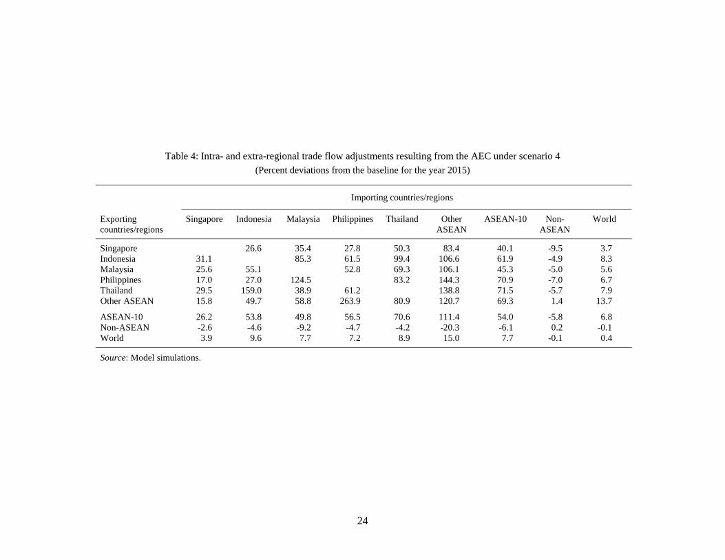
Not surprisingly, intra-ASEAN trade is predicted to increase drastically. The

percent increase in a member’s intra-ASEAN imports is positively correlated with its

initial tariff rates. For example, intra-ASEAN imports of Other ASEAN are estimated to

14 Stone and Struttt (2009) find that trade and transport cost reductions in the Greater Mekong Subregion (GMS) would greatly expand intraregional trade and increase economic welfare of the GMS countries.

12

increase by 111%, whereas those of Singapore increase by only 26%. On average, intra-

ASEAN trade would expand 54% while ASEAN-10’s imports from non-ASEAN countries

would contract by 6.1%. Since world trade flows increase by 0.4%, the extent of trade

creation effects is greater than that of trade diversion.

While Other ASEAN’s imports from all the member states increase significantly,

increases in the Philippines’ imports from Other ASEAN, Indonesia’s imports from

Thailand and Malaysia’s imports from the Philippines stand out. Although changes in trade

flows by sector are not presented in Table 4, these dramatic increases mostly stem from

extraordinarily large increases in bilateral imports of particular products. For example, the

Philippines’ imports of rice, fossil fuel and apparel from Other ASEAN are predicted to

increase by 970%, 163% and 134%, respectively, compared with the baseline in 2015.

However, the enormous increase in rice imports is the main reason for a 264% increase in

the Philippines’ imports from Other ASEAN because rice constitutes about one-fifth of the

former’s imports from the latter. Similarly, a 556% increase in Indonesia’s imports of

processed food from Thailand and over a 1,000% rise in Malaysia’s imports of other crops

from the Philippines are major causes of the drastic increases in Indonesia-Thailand and

Malaysia-Philippines trade, respectively.

4.3 Effects on Sectoral Output

Estimates of the impact of ASEAN integration are provided for the 20 sectors

under scenario 4. The expected changes are again expressed in percent deviations from the

baseline in 2015. Evidently, the differences in the initial tariff rates across sectors play a

critical role in determining the direction of the adjustments in sectoral output. Other factors

that affect the magnitude and direction of output adjustments for each product category

include the import-demand ratio, the export-output ratio, the share of each imported

intermediate input in total costs, and the elasticity of substitution between domestic and

imported products.15

15 A sector with a larger import-demand ratio generally suffers from proportionately larger output contraction through greater import penetration when initial tariff levels are relatively high. In contrast, a sector with a higher export-output ratio typically experiences a larger extent of output expansion, as a result of the removal of tariffs in the member countries. The share of imported intermediate inputs in the

13

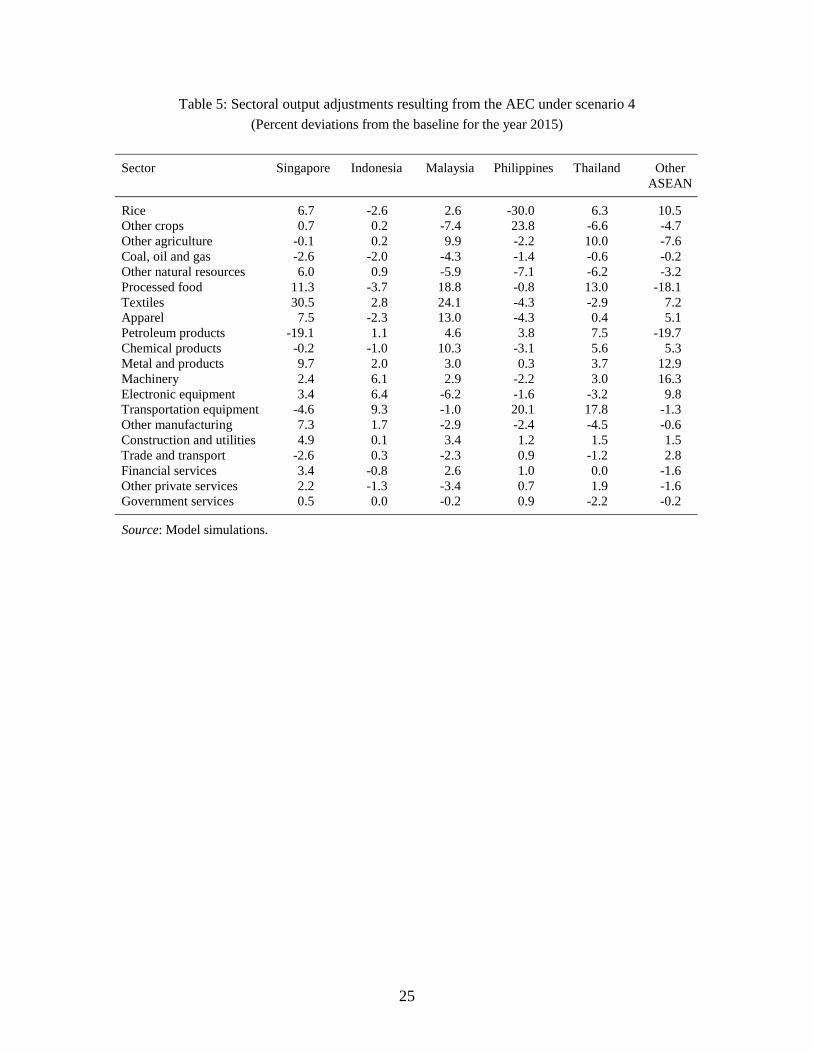
Among agricultural sectors, output of rice in Thailand and Other ASEAN

(particularly Vietnam) and that of other crops in the Philippines expand through large

increases in intra-ASEAN exports. By contrast, output of rice in the Philippines and

Indonesia, as well as that of other crops in Malaysia, Thailand and Other ASEAN, contract

mainly because of large import penetrations resulting from the removal of relatively high

tariffs. Finally, since the share of Singapore’s agricultural sectors in total output is only

0.3%, the results for Singapore are unimportant. Overall, changes in output of agricultural

sectors among the ASEAN members are consistent with a priori expectations.

Sectoral output results for manufacturing and services sectors need to be interpreted

with caution. Output expansions of processed food in Thailand, textiles and apparel in

Other ASEAN, machinery in Singapore and Malaysia, electronic equipment in Singapore,

transportation equipment (mainly motor vehicles) in Thailand and financial services in

Singapore and Malaysia are consistent with comparative advantage of these countries.

However, output expansions of processed food, textiles and apparel in Singapore and

Malaysia and machinery and electronic equipment in Other ASEAN, as well as an output

contraction of electronic equipment in Malaysia, seem to be counter-intuitive and need

some explanations.

The tariff rates on processed food are among the highest in the region except in

Singapore and the Philippines. Thus, a significant increase in Singapore and Malaysia’s

intraregional exports appears to be a major cause for their output expansion of processed

food, including palm oil in Malaysia. Expansions of output in textiles and apparel in the

two countries also results from the elimination of relatively high tariffs in these products,

but absolute increases are very small because textiles and apparel account for less than 1%

and 2%, respectively, of Singapore and Malaysia’s total output. The predicted contraction

of Malaysia’s electronic industry might be explained by a small percent increase in the

exports relative to other industries. Almost 70% of Malaysia’s intra-ASEAN exports of

electronic equipment are shipped to Singapore, while about 60% of its intra-ASEAN total cost of a downstream industry (e.g., the share of imported textiles in the cost of the apparel industry) would evidently affect the magnitude and direction of output adjustments in the latter sector. Finally, the greater the values of substitution elasticities between domestic and imported products, the greater the sensitivity of the import-domestic demand ratio to changes in the relative price of imports, thereby magnifying the effects of regional integration.

14

imports of this product originate from Singapore. Malaysia’s exports of electronic

equipment to Singapore are predicted to increase by only 9.7%, whereas its imports from

Singapore are estimated to increase by 13.6%, which eventually results in a reduction in

demand for domestic electronic equipment in Malaysia.

In the machinery and electronic equipment sectors, international fragmentation has

dramatically developed in East Asia since the 1990s (Ando and Kimura, 2005a; Kimura,

2006). Paralleling this development is a significant rise in the shares of parts and

components in both exports and imports of machinery and electronic equipment in the

region. More specifically, over the 1990-2003 period, intra-East Asian exports of parts and

components of these products increased by 452%, which accounted for about a half of

intraregional export growth (Ando and Kimura, 2005b). Thus, it is quite plausible for

Other ASEAN to expand exports of low-quality machinery and electronic equipment

(including parts and components), imports of high-quality products and output of these

products simultaneously. It should be noted that absolute changes in Other ASEAN’s

output of machinery and electronic equipment are rather small since these products are

projected to constitute only 7% of Other ASEAN’s total output for 2015 in the baseline,

compared with 27% in Singapore, 34% in Malaysia, 20% in the Philippines and 26% in

Thailand.

5. Conclusion

In this paper, we have used a dynamic CGE model to examine the effects of the

ASEAN Economic Community on economic welfare, trade flows and sectoral output of

the member states. The simulation experiments are conducted for four different nested

scenarios, starting with the removal of bilateral tariffs and export taxes/subsidies.

Subsequently, a reduction in frictional trade costs (e.g. administrative and technical

barriers) is examined. In two final scenarios, productivity levels are assumed to be

positively correlated with economic openness, while the incremental effects of lowering

the trade and transport margins are also assessed.

Large disparities in the initial tariff rates across members and the incorporation of

the Armington assumption result in large terms-of-trade effects, particularly for Singapore

15

(positive) and Other ASEAN (negative), which might dominate other welfare effects under

the first scenario. It is found that reductions in frictional trade costs and the trade and

transport margins have large effects on economic welfare while allowing for endogenously

determined productivity levels has a small impact. When these factors are incorporated, the

estimated welfare gains for the year 2015 range from 1.1% in Indonesia to 9.4% in

Thailand. The results suggest that reductions in administrative and technical barriers (e.g.

streamlining customs procedures and mutual recognition of product standards) and

lowering the trade and transport margins (e.g. through increased competition and

improvements in infrastructure) are significant in enlarging the benefits of the AEC.

A challenging extension of the paper would be to endogenize FDI flows to consider

attraction of these flows to ASEAN countries, which may have greater effects than the

removal of trade barriers, as in the cases of Mexico joining NAFTA and Spain and

Portugal joining the EU. Changes in FDI flows deriving from the AEC in the Plummer and

Chia’s (2009) study are estimated to result in an increase in ASEAN’s FDI stocks to the

tune of 28-63 percent ($117-$264 billion relative to 2006 inward FDI stocks).

Endogenizing an FDI effect would require the construction of a world investment matrix

by industry, but the data on bilateral FDI flows by source and host countries and industry

are currently available only in a few developed countries. Nevertheless, such an extension

will allow us to shed new light on the trade-FDI nexus and international production and

distribution networks in the region.

16

Appendix: Values of the Key Elasticities

Most of the elasticities in the LINKAGE model have a long vintage, in some cases

going back to the late 1980s. Many have been gleaned from the literature using

econometric estimates when available. Others can be attributed to guess-estimates.

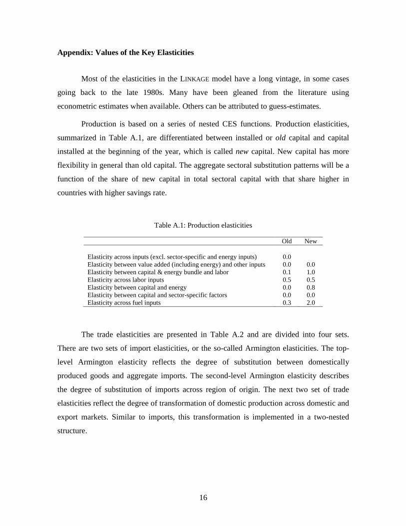
Production is based on a series of nested CES functions. Production elasticities,

summarized in Table A.1, are differentiated between installed or old capital and capital

installed at the beginning of the year, which is called new capital. New capital has more

flexibility in general than old capital. The aggregate sectoral substitution patterns will be a

function of the share of new capital in total sectoral capital with that share higher in

countries with higher savings rate.

Table A.1: Production elasticities Old New

Elasticity across inputs (excl. sector-specific and energy inputs) 0.0 Elasticity between value added (including energy) and other inputs 0.0 0.0 Elasticity between capital & energy bundle and labor 0.1 1.0 Elasticity across labor inputs 0.5 0.5 Elasticity between capital and energy 0.0 0.8 Elasticity between capital and sector-specific factors 0.0 0.0 Elasticity across fuel inputs 0.3 2.0

The trade elasticities are presented in Table A.2 and are divided into four sets.

There are two sets of import elasticities, or the so-called Armington elasticities. The top-

level Armington elasticity reflects the degree of substitution between domestically

produced goods and aggregate imports. The second-level Armington elasticity describes

the degree of substitution of imports across region of origin. The next two set of trade

elasticities reflect the degree of transformation of domestic production across domestic and

export markets. Similar to imports, this transformation is implemented in a two-nested

structure.

17

Table A.2: Trade elasticities

Top-level Armington elasticity Rice 4.45 Other crops 4.36 Other agriculture 3.94 Coal, oil and gas 4.93 Other natural resources 2.80 Processed food 4.01 Textiles 3.94 Apparel 4.27 Petroleum products 4.93 Chemical products 3.94 Metal and products 3.94 Machinery 3.94 Electronic equipment 3.94 Transportation equipment 4.71 Other manufacturing 3.94 Construction and utilities 1.76 Trade and transport 2.09 Financial services 2.09 Other private services 2.09 Government services 2.09 Elasticity of substitution across imports by Twice the value of top-level region of origin Armington elasticity Elasticity of transformation between output supplied domestically and exported Infinity Elasticity of transformation across exports by region of destination Infinity

18

References

Anderson, K., Martin, W., and van der Mensbrugghe, D. (2006). Market and welfare

implications of Doha reform scenarios. In: K. Anderson and W. Martin (eds.), Agricultural Trade Reform and the Doha Development Agenda. New York and Washington, DC: Palgrave Macmillan and World Bank.

Ando, M., and Kimura, F. (2005a). The formation of international production and distribution networks in East Asia. In: T. Ito and A. K. Rose (eds.), International Trade in East Asia. Chicago: University of Chicago Press.

Ando, M., and Kimura, F. (2005b). Global supply chains in machinery trade and sophisticated nature of production/distribution networks in East Asia. KUMQRP Discussion Paper No. 2005-15. Tokyo: Keio University.

Armington, P. (1969). A theory of demand for products distinguished by place of production. IMF Staff Papers, 16, 159-178.

Asian Development Bank (ADB) (2008). Emerging Asian Regionalism. Manila: Asian Development Bank.

Bchir, H., Decreux, Y., Guérin, J-L., and Jean, S. (2002). MIRAGE, A Computable General Equilibrium Model for Trade Policy Analysis. CEPII Working Paper No. 2002-17. Paris: CEPII.

Brown, D. K. (1987). Tariffs, the terms of trade, and national product differentiation. Journal of Policy Modeling, 9, 503-526.

Das, S., Roberts, M. J., and Tybout, J. R. (2007). Market entry costs, producer heterogeneity, and export dynamics. Econometrica, 75, 837-873.

de Melo, J., and Robinson, S. (1992). Productivity and externalities: Models of export-led growth. Journal of International Trade & Economic Development, 1, 41-68.

Dervis, K., de Melo, J., and Robinson, S. (1982). General Equilibrium Models for Development Policy. Cambridge: Cambridge University Press.

Dessus, S., Fukasaku, K., and Safadi, R. (1999). Multilateral Tariff Liberalization and the Developing Countries. OECD Development Centre Policy Brief No. 18. Paris: OECD.

Hertel, T. W., ed. (1997). Global Trade Analysis: Modeling and Applications. Cambridge: Cambridge University Press.

Hoekman, B. (2000). The next round of services negotiations: Identifying priorities and options. Federal Reserve Bank of St. Louis Review, 82(4), 31-48.

Ianchovichina, E., and McDougall, R. (2000). Theoretical Structure of Dynamic GTAP. GTAP Technical Paper No. 17. West Lafayette: Center for Global Trade Analysis, Purdue University.

19

Kawai, M., and Wignaraja, G. (2007). ASEAN+3 or ASEAN+6: Which Way Forward? ADB Institute Discussion Paper No. 77. Tokyo: ADB Institute.

Keuschnigg, C., and Kohler, W. (2002). Eastern enlargement of the EU: How much is it worth for Austria? Review of International Economics, 10, 324-342.

Kimura, F. (2006). International production and distribution networks in East Asia: Eighteen facts, mechanics, and policy implication. Asian Economic Policy Review, 1, 326-344.

Kiyota, K., and Stern, R. M. (2008). Computational Analysis of APEC Trade Liberaliza-tion. RSIE Discussion Paper No. 578, University of Michigan.

Lee, H., and van der Mensbrugghe, D. (2005). Interactions between foreign direct investment and trade in a general equilibrium framework. Paper presented at the ADB Experts’ Meeting on Long-term Scenarios of Asia’s Growth and Trade, Asian Development Bank, Manila, 10-11 November.

Lee, H., and van der Mensbrugghe, D. (2008). Regional integration, sectoral adjustments and natural groupings in East Asia. International Journal of Applied Economics, 5(2), 57-79.

Lluch, C. (1973). The extended linear expenditure system. European Economic Review, 4, 21-32.

Löfgren, H., Harris, R. L., and Robinson, S. (2002). A Standard Computable General Equilibrium (CGE) Model in GAMS. Microcomputers in Policy Research 5. Washington, DC: International Food Policy Research Institute.

Madsen, A. D., and Sorensen, M. L. (2002). Economic consequences for Denmark of EU enlargement. Paper presented at the International Conference on Policy Modeling, Brussels, 4-6 July.

Martin, W., and Mitra, D. (2001). Productivity growth and convergence in agriculture and manufacturing. Economic Development and Cultural Change, 49, 403-422.

Narayanan, B., and Walmsley, T. L. (eds.) (2008). Global Trade, Assistance, and Production: The GTAP 7 Data Base. West Lafayette: Center for Global Trade Analysis, Purdue University.

Plummer, M. G., and Chia, S. Y., eds. (2009). Realizing the ASEAN Economic Community: A Comprehensive Assessment. Singapore: ISEAS.

Samuelson, P. A. (1952). The transfer problem and transport costs: The terms of trade when impediments are absent. Economic Journal, 62, 278-304.

Stone, S., and Strutt, A. (2009), Transport Infrastructure and Trade Facilitation in the Greater Mekong Subregion. ADBI Working Paper No. 130. Tokyo: Asian Development Bank Institute.

20

van der Mensbrugghe, D. (2005). LINKAGE Technical Reference Document: Version 6.0. Washington, DC: World Bank.

van der Mensbrugghe, D. (2006). Estimating the benefits: Why numbers change. In: R. Newfarmer (ed.), Trade, Doha and Development: A Window into the Issues. New York and Washington, DC: Palgrave Macmillan and World Bank.

Verikos, G., and Zhang, X-G. (2001). Global Gains from Liberalizing Trade in Telecom-munications and Financial Services. Staff Research Paper. Canberra: Productivity Commission.

21

Table 1: Regional and sectoral aggregation A. Regional aggregation Country/region Corresponding economies/regions in the GTAP database Singapore Singapore Indonesia Indonesia Malaysia Malaysia Philippines Philippines Thailand Thailand Other ASEAN Brunei, Cambodia, Laos, Myanmar, Vietnam China China, Hong Kong Japan Japan Korea Korea Taiwan Taiwan Australia/New Zealand Australia, New Zealand North America United States, Canada EU and EAFTA EU-27, Iceland, Liechtenstein, Norway, Switzerland Rest of world All the other economies/regions

B. Sectoral aggregation Sector Corresponding commodities/sectors in the GTAP database Rice Paddy rice, processed rice Other crops Wheat, cereal grains nec, vegetables and fruits, oil seeds, sugar cane and sugar beet, plant-based fibers, crops nec Other agriculture Livestock, fishing Coal, oil and gas Coal, oil, gas Natural resources forestry, minerals Food products meat products, dairy products, other food products, beverages and tobacco products Textiles Textiles Apparel Wearing apparel and leather Petroleum products Petroleum and coal products Chemical products Chemical, rubber and plastic products Metal and products Iron and steel, nonferrous metal, fabricated metal products Machinery Machinery and equipment Electronic equipment Electronic equipment Transportation equipment Motor vehicles and parts, other transportation equipment Other manufactures Wood products, paper products, publishing, mineral products, manufactures nec Construction and utilities Construction, public utilities Trade and transport Trade, sea transport, air transport, transport nec Financial services Insurance, financial services nec Other private services Communication, business services, recreation and other services Government services Public administration and defense, education, health services Source: GTAP database, version 7. Note: nec = not elsewhere classified.

22

Table 2: ASEAN countries’ tariff rates on imports from ASEAN members, 2004 (percent)

Sector Singapore Indonesia Malaysia Philippines Thailand Other ASEAN 1 Rice 0.0 18.7 0.0 50.0 0.0 2.4 2 Other crops 0.0 3.3 11.8 4.6 20.6 7.3 3 Other agriculture 0.0 2.7 0.4 2.3 4.1 7.2 4 Coal, oil and gas 0.0 0.0 1.2 3.0 0.0 0.2 5 Other natural resources 0.0 1.5 0.0 2.9 0.2 1.2 6 Processed food 0.0 18.5 19.8 3.6 34.7 21.8 7 Textiles 0.0 2.5 4.4 2.6 12.5 8.9 8 Apparel 0.0 2.2 2.8 4.5 6.4 7.4 9 Petroleum products 0.0 1.3 0.3 1.5 0.7 13.9 10 Chemical products 0.0 2.2 1.4 2.8 6.3 3.9 11 Metal and products 0.0 2.1 2.2 1.5 3.7 3.4 12 Machinery 0.0 1.5 1.8 0.9 2.6 5.5 13 Electronic equipment 0.0 0.6 0.1 0.2 0.9 5.1 14 Transportation equipment 0.0 2.8 5.8 3.8 4.5 22.8 15 Other manufacturing 0.0 2.9 2.0 2.8 10.1 7.3 16 Construction and utilities 0.0 6.0 4.0 15.0 13.5 6.0 17 Trade and transport 2.5 12.0 4.5 17.0 17.0 7.5 18 Financial services 5.6 10.3 11.6 13.8 12.5 17.7 19 Other private services 3.0 21.5 3.5 17.5 17.0 9.5 20 Government services 5.5 10.5 5.5 10.5 13.0 10.5 Weighted average 0.0 3.2 2.4 3.3 4.4 9.4 Sources: Sectors 1-15: GTAP database, version 7. Sectors 16-20: Authors’ calculation based on ad

valorem equivalents of nontariff barriers in Hoekman (2000), Kiyota and Stern (2008), and Verikos and Zhang (2001).

23

Table 3: The welfare effects of the AEC (Deviations in equivalent variations from the baseline in 2015)

Region Scenario 1 Scenario 2 Scenario 3 Scenario 4

A. Absolute deviations (US$ billion in 2004 prices) Singapore 5.25 8.09 8.13 11.16 Indonesia 0.48 1.76 2.06 4.37 Malaysia 2.73 5.37 5.47 8.99 Philippines 1.15 1.80 1.91 2.69 Thailand 1.80 3.50 3.88 7.47 Other ASEAN -1.00 0.10 0.42 2.50 China -0.91 -1.59 -0.99 -1.62 Japan -0.30 -0.84 -0.65 -1.07 Korea 0.04 -0.29 -0.21 -0.54 Taiwan -0.11 -0.31 -0.27 -0.39 Australia/New Zealand -0.45 -0.51 -0.46 -0.60 North America -0.42 -0.79 -0.50 -0.89 EU and EFTA -0.37 -1.43 -1.08 -1.99 Rest of world -1.13 -1.59 -1.12 -1.55 ASEAN-10 10.41 20.61 21.88 37.19 World 6.76 13.26 16.60 28.54 B. Percent deviations Singapore 3.83 5.90 5.93 8.14 Indonesia 0.12 0.46 0.53 1.13 Malaysia 1.72 3.38 3.45 5.66 Philippines 1.01 1.58 1.67 2.35 Thailand 2.26 4.39 4.87 9.38 Other ASEAN -0.94 0.09 0.39 2.33 China -0.03 -0.05 -0.03 -0.05 Japan -0.01 -0.02 -0.02 -0.03 Korea 0.00 -0.03 -0.02 -0.06 Taiwan -0.03 -0.08 -0.07 -0.10 Australia/New Zealand -0.06 -0.07 -0.06 -0.08 North America 0.00 -0.01 0.00 -0.01 EU and EFTA 0.00 -0.01 -0.01 -0.02 Rest of world -0.01 -0.02 -0.01 -0.02 ASEAN-10 1.06 2.10 2.23 3.78 World 0.02 0.03 0.04 0.07

Definitions of scenarios: Scenario 1: The ASEAN members remove bilateral tariffs and export taxes/subsidies by 2015. The sector-

specific productivity factors related to openness (χi,t) are fixed at the baseline levels. Scenario 2: Scenario 1 plus a 2.5% reduction in administrative and technical barriers among the ASEAN

members over the period 2010-2015. χi,t are fixed at the baseline levels. Scenario 3: Same as scenario 2 except that χi,t are endogenous and determined by equation (2). Scenario 4: Scenario 3 plus a 10% reduction in the trade and transport margins among the ASEAN

countries over the period 2010-2015. Source: Model simulations.

24

Table 4: Intra- and extra-regional trade flow adjustments resulting from the AEC under scenario 4 (Percent deviations from the baseline for the year 2015)

Importing countries/regions

Exporting Singapore Indonesia Malaysia Philippines Thailand Other ASEAN-10 Non- World countries/regions ASEAN ASEAN Singapore 26.6 35.4 27.8 50.3 83.4 40.1 -9.5 3.7 Indonesia 31.1 85.3 61.5 99.4 106.6 61.9 -4.9 8.3 Malaysia 25.6 55.1 52.8 69.3 106.1 45.3 -5.0 5.6 Philippines 17.0 27.0 124.5 83.2 144.3 70.9 -7.0 6.7 Thailand 29.5 159.0 38.9 61.2 138.8 71.5 -5.7 7.9 Other ASEAN 15.8 49.7 58.8 263.9 80.9 120.7 69.3 1.4 13.7

ASEAN-10 26.2 53.8 49.8 56.5 70.6 111.4 54.0 -5.8 6.8 Non-ASEAN -2.6 -4.6 -9.2 -4.7 -4.2 -20.3 -6.1 0.2 -0.1 World 3.9 9.6 7.7 7.2 8.9 15.0 7.7 -0.1 0.4 Source: Model simulations.

25

Table 5: Sectoral output adjustments resulting from the AEC under scenario 4 (Percent deviations from the baseline for the year 2015)

Sector Singapore Indonesia Malaysia Philippines Thailand Other ASEAN Rice 6.7 -2.6 2.6 -30.0 6.3 10.5 Other crops 0.7 0.2 -7.4 23.8 -6.6 -4.7 Other agriculture -0.1 0.2 9.9 -2.2 10.0 -7.6 Coal, oil and gas -2.6 -2.0 -4.3 -1.4 -0.6 -0.2 Other natural resources 6.0 0.9 -5.9 -7.1 -6.2 -3.2 Processed food 11.3 -3.7 18.8 -0.8 13.0 -18.1 Textiles 30.5 2.8 24.1 -4.3 -2.9 7.2 Apparel 7.5 -2.3 13.0 -4.3 0.4 5.1 Petroleum products -19.1 1.1 4.6 3.8 7.5 -19.7 Chemical products -0.2 -1.0 10.3 -3.1 5.6 5.3 Metal and products 9.7 2.0 3.0 0.3 3.7 12.9 Machinery 2.4 6.1 2.9 -2.2 3.0 16.3 Electronic equipment 3.4 6.4 -6.2 -1.6 -3.2 9.8 Transportation equipment -4.6 9.3 -1.0 20.1 17.8 -1.3 Other manufacturing 7.3 1.7 -2.9 -2.4 -4.5 -0.6 Construction and utilities 4.9 0.1 3.4 1.2 1.5 1.5 Trade and transport -2.6 0.3 -2.3 0.9 -1.2 2.8 Financial services 3.4 -0.8 2.6 1.0 0.0 -1.6 Other private services 2.2 -1.3 -3.4 0.7 1.9 -1.6 Government services 0.5 0.0 -0.2 0.9 -2.2 -0.2

Source: Model simulations.