estimating the mean of random binomial parameterthe investigation of j. vanryzinwassupportedin...

ESTIMATING THE MEAN OF ARANDOM BINOMIAL PARAMETER

G. MORRIS SOUTHWARDINTERNATIONAL PACIFIC HALIBUT COMMISSION

andJ. VAN RYZIN

UNIVERSITY OF WISCONSIN

1. Introduction

In studying biological phenomenon, one often observes random variables whichare the result of other randomly occurring unobservable events. This is usuallythe case in the observation of genetic traits. The measurable trait in questionhas a probability distribution for the population of animals under study. Eachindividual member of the population of animals carries a value of the measurabletrait, but it may or may not (and often is not) directly observable. It is not diffi-cult to envision the probability distribution of the trait in the population as beingcontinuous, while the distribution of the visible expression of the trait is a dis-crete count depending on the value of the measurable trait.Such a problem came to the authors' attention during discussion with a poultry

scientist who was interested in the probability distribution governing the fre-quency with which blood spotted eggs occur. Poultrymen wish to determine fromexamination of a small number of eggs laid early in the life of each hen what theaverage probability of laying blood spotted eggs is for the flock.The problem can be conceptualized as follows. The distribution of blood spots

in eggs for a given chicken is taken as binomial. That is, if p represents the prob-ability of a given chicken to lay a blood spotted egg and m eggs are laid, thenX = number of blood spotted eggs is binomially distributed with parameters mand p assuming the eggs are laid independently. However, the probability p (orpropensity) for laying blood spotted eggs (the trait in question), differs fromchicken to chicken and can be thought of as having a continuous distributionon the unit interval. The probability distribution of the blood spotting trait pin the population is not directly observable. That is, one might postulate that thebinomial parameter p (or trait) has a distribution on the unit interval and thatthe values of this probability carried by each bird in the flock are independentlyallocated according to this distribution, denoted G(p). Rarely, if ever, are valuesof p directly observable.The investigation of J. Van Ryzin was supported in part by USPHS Research Grant No.

GM-10525-08, National Institute of Health, Public Health Service, and in part by NSFContract No. GP-9324.

249

250 SIXTH BERKELEY SYMPOSIUM: SOUTHWARD AND VAN RYZIN

Thus, the model is written as

(1.1) f(x; m) = | (m) px(1 - p)m-z dG(p),

x = 0, * , m, where m is the size of the sample examined and G(p) is the dis-tribution of the probability p.The problem we consider here is that of estimating the mean g,u of the prob-

ability distribution G(p), that is, u = ,u = f p dG(p), based on a random sampleXi, * * *, X. from f(x; m), where Xi is the number of blood spotted eggs amongthe m eggs sampled from the ith chicken. The moment estimator of J,u and itslarge sample properties along with confidence intervals are developed in Section2.

It is clear that the above type of sampling, when we wish to estimate y,occurs in many setups similar to that of our chicken example. Also, the alliedproblem, when the sample size m is allowed to vary from individual to individual,is discussed in Sections 3, 4, and 5. In that case, the distribution of each Xi isgiven by equation (1.1), where m is now replaced by mi; that is, Xi is distributedwith discrete densityf(xi; mi) in (1.1), xi = 0, * , mi, i = 1, * * *, n.Theorems 5.1 and 5.2 develop the consistency and asymptotic distribution

theory for the case of differing sample sizes (mi different). These theorems con-cern an estimator 4 for uL which behaves asymptotically like the minimum vari-ance unbiased linear (in the Xi) estimator of A which is studied in Section 3.Some aspects of this general problem are covered by Pearson [2] who discusses

Bayes theorem in the light of experimental sampling. However, no attack on theabove problem is made therein.

2. Estimation of the mean of G(p)

Let Xi, * , X, be a random sample from the model

(2.1) f(x;m) = f () px(l - p)m- dG(p).

We consider the problem of estimating the mean

(2.2) = p dG(p)based only on the observations X1,i , Xn. Note that in fact there exists abivariate random sample {(Xi, Pi), i 1, . .. , n}, where we assume that Xiconditional on Pi = p is binomially distributed with m trials and success prob-ability p and the Pi are independent marginally distributed as G(p). We writeXilPi = p - b(m, p) and Pi - G(p), i = 1, * -*-, n.We employ the method of moments to obtain our estimator. Observe that

(2.3) E(X1) = E{E[X,IPi]} = mE(P1) = mI

From (2.3) and the fact that X1, * *, Xn are independent and identically dis-

MEAN OF A RANDOM BINOMIAL PARAMETER 251

tributed with distribution (2.1), we have EX = my. Hence, the method of mo-ments yields the estimator a of Iu given by

(2.4) Ximn mn i=l

From the strong law of large numbers, we have immediately that a is a stronglyconsistent estimator of I. That is,(2.5) P(lim p)=1.

Next we will obtain the large sample distribution of 4a quite directly from thecentral limit theorem. First, observe that the variance of A is given by

(2.6) Var (A) = Var (m) =

where Ad = Var (X1). Therefore, by the central limit theorem for independent,identically distributed random variables with finite variance, we have as nX

(2.7) s 4 - -)N(O, 1),

where S(Zn) - N(,u, a2) means {Zn} converges in distribution to a random vari-able Z which is normally distributed with mean ,u and variance o2.

Besides 4 being strongly consistent as in (2.5) and asymptotically normal asin (2.7), we note that a in (2.4) is the minimum variance unbiased linear (in theXi) estimator of ,u. This is a direct result of Theorem 3.1 in Section 3.

Furthermore, by definingn

(2.8) S2 = (n - 1)- (X, 2,

we have S2 in an unbiased, consistent estimator of al. That is,

(2.9) 32 d

as n -4 o. Using (2.9) and (2.7), we obtain (see for example, Rao [3], (x) - (b),p. 102) as n- oo

(2.10) (mvn(4 - )) -N(0, 1).

From (2.10), we can immediately give a 100(1 - a) per cent, 0 < a < 1,large sample confidence interval for p, since

(2.11) lim P - Za/2 <p < ( + 1 Z"/ = 1-a,n m-+/2'

where Za/2 is defined by the equation

(2.12) f (2!-) exp { } dt = 1 - a.

For example, if we want a 95 per cent confidence interval for the mean prob-


ability of the flock for laying a blood spotted egg, we would choose a = 0.05yielding an approximate large sample confidence interval

(2.13) (±(X 3 )1(X+ l 96S))

Some sample intervals are constructed for data randomly generated by a sim-ilation process involving varying sample sizes and are here included.The density given by (2.1) was computed for the case of G(p) being a beta

distribution. That is, assume dG(p) = g(p) dp, where the density g(p) is given by(2.14) g(p) = {(r, s)}ppl(l - p)&A, 0 < p < 1, r > 0, s > 0,and f3(r, s) = fo pr-1(l - p) - dp. A range of values of m, r, and s was chosenand ,u computed for each set of values thereof. Random samples were drawn andA and Var (4) estimated. Table I gives u, 4, and the estimated standard errorof A, S/(mVn), for a few selected values of m, r, and s. The entry on the first lineis for a sample of n = 50 and on the second line for a sample of n = 200. Inmost instances A estimates uz well; p i: 1.96S/mV/n fails to contain Iu only threetimes out of the 40 cases presented. That is, when m = 10, r = s = 1, n = 50;m = 15, r = 1, s = 5, n = 200; and m = 15, r = 2, s = 15, n = 200. Manyother values of m, r, s, and n were also tried with similar good results.

3. The case of differing sample sizes

Often times in applications the number of trials m connected with each ob-servation may not be the same. That is, consider the case where each X, isdistributed as (2.1) with m replaced by mi, i = 1, * - *, n. We assume the mi areall known, fixed, positive integers, but not necessarily equal.To estimate Iu, we again use the method of moments. Similar to (2.3), we have

(3.1) E(Xi) = mig, i= 1, ** *, n.

Since (3.1) implies both E{jF_?.. (Xi/mj)} = nu and E(E2'1 Xi) = (_t=l mi)p,we have as possible moment estimators of ,u both

(3.2) al nand

x(3.3) 42==mwhere m = (1/n) Et-l mi.

In order to discuss the relative merits of the estimators A, and 42, we computetheir variances. With(3.4) 2 = Var (Pi) = f (p -)2 dG(p)and(3.5) X = E{P1(1 - PI)} = f p(l - p) dG(p),


TABLE I

COMPARISON OF ,U AND }X FOR CASE OF BETADISTRIBUTION, n = 50 AND n = 200

m r 8 4PAP S/(m/Vn)

10 1 1 .500 .594 .0411.505 .0217

2 .333 .314 .0366.342 .0198

5 .167 .170 .0241.158 .0125

10 .091 .100 .0204.093 .0087

15 .063 .060 .0121.060 .0068

2 1 .667 .698 .0366.688 .0177

2 .500 .548 .0388.482 .0181

5 .286 .314 .0287.298 .0146

10 .167 .178 .0225.154 .0106

15 .118 .120 .0232.116 .0082

15 1 1 .500 .489 .0470.474 .0218

2 .333 .295 .0397.327 .0179

5 .167 .197 .0268.190 .0129

10 .091 .116 .0209.096 .0082

15 .063 .052 .0107.062 .0057

2 1 .667 .653 .0341.657 .0183

2 .500 .449 .0386.485 .0165

5 .286 .320 .0306.285 .0136

10 .167 .192 .0225.167 .0102

15 .118 .112 .0175.118 .0075

we have

(3.6) Var (A2) = (Mn)-2 E Var (Xi)

= n-'(ana2 + b.7r),where an = (m2n)1-I = 1 Xbn = (rn)-1, r7i = n-1 Et?_ 1 Mi.


Also, we obtainn

(3.7) Var (Al) = n-2 E Var (Xi) = n-(c(a2 + cnr),

where Cn = n-1 mT1.From the Cauchy-Schwarz inequality, it is easy to show that

(3.8) an _ 1 and bn Cn,

where the inequalities are strict unless mi = m for all i. Hence, it is clear thatneither A, nor #2 is for all G relatively more efficient than the other. In fact, from(3.8) we see that if a2 = 0 and r > 0, A2 is more efficient, Var (#2) . Var (Al),than Al, while the reverse is true if o2> 0 and T = 0.Note the case a2 = 0 implies that G(p) is degenerate at, say, p0, and hence

that S. = Et-l Xi is binomially distributed with parameter E-l.I mi and p0.Thus, A2 in this case becomes the classical (maximum likelihood, moment andminimum variance unbiased estimator) solution to the problem of estimatingit = po. In the remainder of the paper, we omit this case from consideration and shallassume 2 > 0.We consider now the question of the existence of an optimal solution in the

minimum variance sense. The following theorem gives a solution to the problemfor unbiased linear (in Xi) estimators.

Let Mn be the class of all unbiased linear estimators of p based on Xi, * , Xn.That is,

(3.9) Mn = {ala = Cmi L Cin =

Observe that the condition Et-I Cin = 1 implies that A is unbiased by (3.1).Also, A E Mn is clearly linear in the Xi as well as in the Xi/mi by taking c;n =Cin/mi and defining A = 2-1i cinXi in Mn.THEOREM 3.1. The minimum variance unbiased linear estimate of , (that is,

the A E Mn of minimum variance) is given by

(3.10) AO = Ecn m'

where

(3.11) 4n = cfn(ol2,) = {2 + m-} /i { +

with a2 and r as in (3.4) and (3.5).REMARK. In particular, Ao = Al = A2 if all mi = m (see Section 1), and AO =

Al if r-2 > 0, r = 0, and Ao = A2 if a2 = 0, T > 0.PROOF. Let oi = Var (Xi/mi) = u2 + r/mi. Then, for A E Mn, we have

Var (p) = ff=l cZ which is minimized by taking cm = 4n as in (3.11). (Seefor example, Rao [3], 2.2, p. 249.)THEOREM 3.2. If .2 > 0, then P{imn- Ao =AO } = 1 for any sequence {mn}

of positive integers.


PROOF. Let Yi = rt-2(Xi/mj), where cr, = Var (Xi/m,) = a2 + r/mi. Lebn = Etn 1 as 2 and observe that (see Loeve [1], 16.3, II, A, p. 238) Po -, =bn-1 Ein 1 (Yi - EY) -- 0 with probability 1 as n -f X provided

(3.12) E_ bn-2 Var (Yn) < oo.n=l

But since bn 2 n(o2 + 7)-1 and Var (Yi) = aS 2 < a-2 we see that (3.12) holdssince n-1n-2 < oo.THEOREM 3.3. If o2 > a, then for any sequence of positive integers {mn},

(3.13) (( ;A') -- N(0, 1)as n -÷ o, where

(3.14) Var (4o) n{ as 2} = { (u2 + T/Mi) -

PROOF. Let Yin = ci,n(milXi- I), ain = Var (Yin), and en = E2?= atn.Then, by an extended version of the Liapounov theorem (Loeve [1], 20.1, a,p. 277), we have

(3.15) ((Var (A'oP) =

OS(Sn) - N(0, 1)as n -X provided

n(3.16) Sn 3 E Elyinl' > O

i=1

as n -X o. But since sn = fias2}-1 and c'n = stor2 with ol = u2 +r/mi ,we have

(3.17) Sn- ElYi = n E a 6E -

- n E ai=1

_ n-%(2 + T)%a4,

where the last inequality follows by using (a2 + r)1 _ at2 < a-2 Hence, (3.16)holds and the theorem is proved.We note that Theorem 3.3 immediately yields large sample confidence inter-

vals on ,u provided C2 and r are known. Under the condition of Theorem 3.3 a100(1- a) per cent large sample approximate confidence interval for ju is givenby(3.18) (o -en,4o+ en),where En = Z./2{_2- (a2 + r/mi)-1} and Ao = _?=ict- (X1/mS). However, inmost applications a2 and T remain unknown and we must therefore concernourselves with this case. Section 4 discusses the question of estimating U2 and T,


while Section 5 develops the necessary large sample results for estimating u whena2 and T are unknown and the sample sizes mi differ.

4. Estimation of a2 and r

Define the random variables Yi, Z. and the indicator variables bi, i = 1, **,n, as follows:

(4.1) Yi =

(4.2) Zi = mt(mi-if mi > 1,

if mi = 1,and

4= { if mi > 1,(4-3) aito if mi = 1.

Observing that EXV = EXi(Xj - 1) + EXi = mWE(P) + miT, one obtains(4.4) EZi=Sir=Furthermore, using the relationship

n ~~~~n(4-5) E(Yi - F)2 = (Yi - ,u)2 - n(Y - i)2it can easily be shown that

(4.6) E (Yi - F)2} = (n - 1){a2+ ( - )T}From equations (4.4) and (4.6) and defining(4-7) ~~~~S2= (n - )lE(Ys - )2

s=land

(4.8) an= max { 5a,

we obtain as moment estimators of r and ca2, when t.i > 0,n

(4.9) T= an1 Zii=l

and

(4.10) (a*)2 = S 2

Note that from (4.4) and (4.6) the unbiasedness of T and (a*)2 follows. That is,when 2-E 5i > 0,(4.11) E(T) = T, E{(a*)2} = 2.The estimator (cr*)2 in (4.9) may be negative as an estimator of a2 > 0. We


shall find it convenient to modify (a*)2 for later purposes and we define 62 as thefollowing positive truncation of (a*) 2,(4.12) 62 = max {(a*) 2, n-11.The following theorem gives the consistency properties of TX 62 (and (a*)2)-THEOREM 4.1. Let C2 > 0. If {mn} is any sequence of positive integers for

which an°-o as n-oo (see (4.8)), then as n ->ooTo T and 62-a2 (or(a * 2) in probability. Furthermore, if {mn} is such that n an2 <an theconvergences hold with probability one.

PROOF. Observe that since 0 < Zi _ 12, we haven

(4.13) Var (T) = an2 E Vi Var (Zi) < (4an)-1.i=l

Hence, T--T- in probability as n -X 00 by Chebyshev's inequality. To prove con-vergence with probability one for T, it suffices (by LoNve [1], 16.3, II, A, p. 238)to verify that n a;2 Var (Zn) <00, which clearly holds in ,n= 1 an2 <00,since Var (Zn) _ 4Observe that (a*)2 is linear in T in (4.10). Thus, convergence of (aT*)2 to CT2 in

probability () or with probability one ( ) as n -X00 follows from Theorem 3.2provided

(4.14) - ( T2+ -) a 0n itimi

as n oo. But (4.14) follows immediately from (4.5), (4.6), and (4.7) providedas n -o,

(4.15) - E (Y 2 2 + ni-m

Let Xt = (Y - U)2 in (4.15) and write the left side of (4.15) as n-11n (X -EX'). Now, applying a version of the Kolmogorov strong law of

large numbers (see Loeve [1], 16.3, II, A, p. 238), we see (4.15) holds provided

(4.16) EI n-2 Var (X') < oo.n=1

But the convergence of the series in (4.16) is an immediate consequence of theboundedness of Xn by one. Thus, the theorem is proved.REMARK. We observe that the condition an -*00 is necessary in Theorem

4.1. To see this consider the case where all the mi are 1 or 2. Then an -,4 oo impliesthere exist no such that an = 0 (Mn = 1) for n _ no. Thus T = az1 St=, Zi for

Pall n _ nO and clearly T rT as n -* oo.

5. Estimation of ,u when C2 and r are unknown in the differingsample size case

The minimum variance unbiased linear estimate of ,u in Theorem 3.1 dependson knowing a2 and r for the optimal choice of the constants Ci' in (3.11). To over-


come this problem when a2 and T are unknown, we propose and study an esti-mator of A, denoted A4, which chooses the cr,, in (3.11) based on the estimators&2X T Of o2, T given in the previous section. Theorems 5.1 and 5.2 give the largesample properties of the proposed estimator.

Specifically, let1 if ? = 0,n

(5-1) ein= Cf(2T) = (2 + if T >,

n

where iand &2 are defined by (4.9), (4.10), and (4.12). Now define

(5.2) -= Cin --

It will be shown that under appropriate conditions 4-4As in probability asn - X (see Theorem 5.1). Before proving this theorem, however, we developthe following lemma.LEMMA 5.1. If o.2 > 0 and an-- °o as n - oo (see (4.3) and (4.8)), then

(53) A0~~I* = AO + (&2 _ ,2) a )(5.3)M(=1ain#

n

+ (0- )

+ [1&2 - u21 + IT - TI]2Ov(1)p1,where ain and #Bin are nonrandom coefficients such that ,i = 1 Cin = 1 (3i = 0and Op(1) indicates a random factor which is bounded in probability.PROOF. Let

(u, v) = {E (u + V)y}l (u + v)1

(5.4) ain = Oc,O1u u =a2,1=T

#innOiV lU=r2,V=r

Observe that cin (u, v) has continuous second order partial (and mixed partial)derivatives on the set {(u, v): 0 < u < oo, 0 _ v < oo}, where the partial deriv-ative is defined from the right at v = 0. Hence, we have the following secondorder Taylor expansion for cin (6&2, T),(5.5) Cin(62, T) = Cin(u2, r) + (a2- n2)an + (T-)lin

(62 - o.2)2 02cin,2 0U2 Iu=?Ul =V


+ (82 2)(^ -T) 02Cs

(T - r) 2 a2Ci;,|+ 2 V2 lu=X*.=#

where min (a2, a2) _ u* < max (a-2, &2) and min (r, T) _ vt < max (T, T). Ob-serve that

{(+ -I)n (U + V)-2}-( + V2j= ( +

(5.6) dj= {3 ( + }

(5.7){( V )-I n +( V )-2} { 1 ( v -2 n (

dv { (u + m }

d92 n2 (u + 2 + m-) .- +(5.8)0u ~(±mS)1 {iEl (~+ m

+(2+ )1 {E (u +-)}} 2 (+ V)-2n ( +

mi j= 1 j= mij=1 j

{ E (u + m }{.E(U + )-) }V

C2C m2 (u + 2_ + E$A 2 ( +(5.8) {- (1+m-) {

~~~)1(n+ ( V )-2}2 2( v )-2 n

1(~+

-

{; (u + }{.n (u + )-)V}and

(.210 I - + m-) 2 (u+m-) m(u +-)jOO (u + m{ ( +m

+ (u + ) E (U +V )-21 ( + V)-2 n ( V )-2+ n{ (U+_n} +; V 1

(5.9)~ ~M, (u nm-) } {Vj u+1-)2


+2 + V)-1 {~n (u + Vm-2}{ 1n (u +;-V(u + -

( V )-2 n =1 ( V)-

{2 (U+(V+ }

Note that from (5.6) and (5.7), we see that ,?=i ai, = X?=i 8i. = 0. Thus, wehave from (5.2) and the Taylor expansion (5.5),

(5.11) AO + (82 - o.2) i( - -)+(T -

(&2 - o.2)2 n X. /a2ei7'2 ,=1 m, \0u2 |u2 8OXa2) ,-t) m-(a |f=*.=)

+ - T)2a 7-)n X

+ 2 ~&i=m,\ 0v2 ts=tsMi =v)

But the right side of (5.11) is bounded by

(5.12) {Ia2 - a21 + If - r1}2 {(_5(u)-)-} ,

where u = maxi ui*, u = mini u*, and v = maxi v*, since from (5.8) through(5.10) and repeated use of the inequalities

(5.13) (u* + vt)-1 _ (t' + )-i _ (ut*)-, <_1<

it is easy to show that

au2 =n(u4 + vj')-1'(5.14) t(tl=X*. =s)-nu()v)

|( V2 lU=+*vvi) (t + 1t)and

(5.15) J(2Clu=u.'v I <-n(u+)-3\au av7'7?7-*I n( + 1)iBounding the right side of (5.11) by (5.12) and noting that Theorem 4.1

implies that as n -,

(5.16) (ui + -)' (0f2 + T)->we have that 5(u)-3(-u + v) is O,(1). Hence, the lemma is proved.


THEOREM 5.1. If 2> 0 and a. -- X as n o (see (4.3) and (4.8)), then po*P

defined by (5.1) and (5.2) is such that A ,uas n oo.PROOF. Repeated use of (u2 + 7)1 _ (o2 + Tim.)1 < a2 and mF 1 _ 1

in (5.6) and (5.7) imply E_el lai.1 and E =-1 Winl are bounded by -4(c2 + 7)-i.Hence, bounding (Xi/mi) - il _ 1 in (5.3) and invoking the convergences inTheorems 3.2 and 4.1, expansion (5.3) yields the result.

LEMMA 5.2. If nma,-1 -l> 0 as n -X 00, then nY(2 - a2) 0 andnX(f-7) AOas n ->Xo.PROOF. From (4.2) we have 0 - Zi _ Y and Var (Zi) _ Y and therefore,

(5.17) Var (nyT) = n%an 2E i Var (Zi) <. n%a1.

Thus, by Chebyshev's inequality, we have(5.18) nYi(T- T) A 0as n -X oo.

Next, in (4.5) and (4.7) observe that

(5.19) (n-1)S n= -i=l

Since S is a nonnegative random variable and IY- < 1, it follows that

(5.20) Var (Sf) < ES1 _ ( 2n 1) Var (Y)

(n-)2 n (a2 + 1n 7m.

But this inequality together with mF 1 < 1 imply that Var (niS2) isO(n-((a2 + r)). Hence, again by Chebyshev's inequality and (4.6), we have

(5.21) ny{ [a + ( - )]

as n -* oo. This result together with (5.18) combine in (4.10) to yieldnY4[(*)2 - or2] A 0 as n -X 00 which completes the proof of the lemma by usingthe definition of 62.THEOREM 5.2. If an --Xo and nan;1 -o 0 as n -X00 (see (4.3) and (4.8)) and

a2 > 0, then(5.22) ((a ())4) N(0, 1)

as n -*oo. Furthermore, replacingVar (no) i/ [ ( + m

by(5.23) u2=

the result (5.22) still holds.


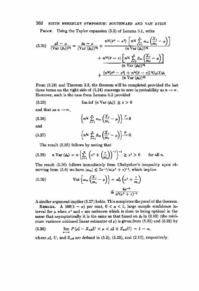
PROOF. Using the Taylor expansion (5.3) of Lemma 5.1, write

5 24 °-y _ ,.-IU n(a2 2) n i-(5.24) (Var (4o~))~ (Var aO (nVar(jZ))6

+ n3( - T) [ni tE1 'h" -m )

(n Var (ao))iM{n5224- *2I + nA -- +}2Ov(l)i2.

(n Var (Ao))AFrom (5.24) and Theorem 3.3, the theorem will be completed provided the lastthree terms on the right side of (5.24) converge to zero in probability as n oo .

However, such is the case from Lemma 5.2 provided(5.25) lim inf {n Var (4o)} _ c > 0

and that as n -,

(5.26) {n nE .ain (xi -)}A°

and

(5.27) {n Eflin - )°The result (5.25) follows by noting that

(5.28) n Var (so) = n {n (.2 (m))} 2 > 0 for all n.

The result (5.26) follows immediately from Chebyshev's inequality upon ob-serving from (5.6) we have lai.1 : 2o&-4/n(0f2 + 7T)-1, which implies

(5.29) Var {ain (m--i- = n (a +in

4a-6S'n2(a2 + r)-2

A similar argument implies (5.27) holds. This completes the proof of the theorem.REMARK. A 100(1- a) per cent, 0 < a < 1, large sample confidence in-

terval for ,u when 0.2 and r are unknown which is close to being optimal in thesense that asymptotically it is the same as that based on AO in (3.10) (the mini-mum variance unbiased linear estimator of p) is given from (5.22) and (5.23) by(5.30) lim P{jy-Za,2U < , <,s0 + Z/2U} =1-a,

ndwhere ;40, U, and Ze./2 are defined in (5.2), (5.23), and (2.12), respectively.


6. SummaryThis paper has examined the question of estimating the mean ;I in (2.2) of a

random binomial parameter having distribution G(p). Such a problem arose inthe context of measuring an unobservable genetic trait in flocks of chickens.The sampling scheme upon which our procedures are based involves observationsXi from a density f(xi; mi) given by (1.1), i = 1, * * *, n, where the mi areknown, fixed, positive integers. The case in which mi = m for i = 1, . .. , n istreated in Section 2 with the confidence intervals for ,u being given by (2.11)based on the estimator a in (2.4).The case in which the mi differ is developed in Sections 3, 4, and 5 with the

corresponding confidence interval for jz given by (3.18) based on Ao in (3.10)of o.2 and T are known and by (5.30) based on uo* in (5.2) if a2 and r are unknown.

> K K > KThe authors would like to thank Mr. Alin-Chiang Wang for doing the com-

puter programming of the simulation results in Section 2.

REFERENCES

[1] M. LohvE, Probability Theory, Princeton, Van Nostrand, 1960 (2nd ed.).[2] E. S. PEARSON, "Bayes theorem in the light of experimental sampling," Biometrika, Vol.

17 (1925), pp. 388-442.[3] C. R. RAO, Linear Statistical Inference and Its Applications, New York, Wiley, 1965.

estimating the mean of random binomial parameterthe investigation of j. vanryzinwassupportedin...

Documents