estimating the long-term health impact of air pollution using spatial ecological studies · ·...

Estimating the long-term health impactof air pollution using spatial ecologicalstudies

Duncan Lee

EPSRC and RSS workshop 12th September 2014

Acknowledgements

This is joint work with Alastair Rushworth and RichardMitchell from the University of Glasgow and Sujit Sahuand Sabyasachi Mukhopadhyay from the University ofSouthampton, and Paul Agnew, Christophe Sarran, FionaO’Connor and Rachel McInnes from the Met Office.

The work is funded by the EPSRC grants EP/J017442/1and EP/J017485/1.

1. Introduction 2. Spatial ecological Studies 3. Modelling 5. Conclusions 2/28

1. Introduction

Air pollution has long been known to adversely affectpublic health, in both the developed and developing world.

A recent report by the UK government estimates thatparticulate matter alone reduces life expectancy by 6months, with a health cost of £19 billion per year.

Epidemiological studies into the effects of air pollutionhave been conducted since the 1990s, with one of the firstbeing that conducted by Schwartz and Marcus (1990) inLondon.

Since 1990 a large number of studies have been conducted,which collectively have investigated the short-term andlong-term health impact of air pollution.


Study designs

Pollution legislation continues to be informed byepidemiological studies investigating both the short-term andlong-term health effects of air pollution exposure.

Acute studies investigate the effects resulting from a fewdays of high exposure.

e.g. NMMAPS in the USA, Dominici et al(2002) and APHEA in Europe, Katsouyanniet al (2001).

Chronic studies investigate the effects of cumulative(long-term) exposure over months and years.

e.g. Dockery et al (1993) in six US cities, andElliot et al (2007) in the UK.


Chronic studies

There are two main study designs when investigating the effectsof long-term exposure to air pollution.

Cohort studies e.g. The Six Cities study by Dockery et al(1993) and the American Cancer study by Pope etal (2002), which relate average air pollutionconcentrations to the health status of a largepre-defined cohort of people.

Spatial ecological studies e.g. Elliot et al (2007) and Lee et al(2009), which relate yearly average air pollutionconcentrations in a set of contiguous areas (such aselectoral wards), against yearly numbers of healthevents from the population living in that area.


2. Spatial ecological studies

Spatial ecological studies relate to populations living in aset of n non-overlapping areal units, rather than toindividuals.

Examples of such studies include Jerrett et al. (2005),Elliott et al. (2007), Lee et al. (2009) and Greven et al.(2011).

The health data are denoted by Y = (Y1, . . . ,Yn) andE = (E1, . . . ,En), which are the observed and expectednumbers of disease cases in each areal unit over a year.

The expected numbers of cases are computed usingexternal standardisation, based on age and sex specificdisease rates.


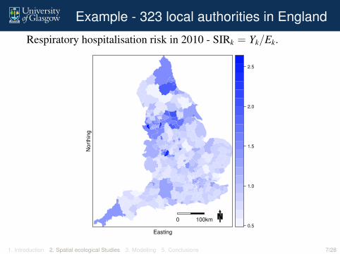
Example - 323 local authorities in England

Respiratory hospitalisation risk in 2010 - SIRk = Yk/Ek.

Easting

Nort

hin

g

0 100km0.5

1.0

1.5

2.0

2.5


Pollution data

Pollution data comes from two distinct sources.

Observed data from the AURN network at single fixedgeographical points located throughout the study region.These data are known to be measured with little error butdo not provide complete spatial coverage of England.

Estimated background concentrations over 12 Kilometregrid cells from the Air Quality in the Unified Model(AQUM) run by the Met Office. These model estimatesprovide complete spatial coverage of the study region, butare known to contain biases and are less accurate then themonitoring data.

Both data sets can be available at an hourly resolution.


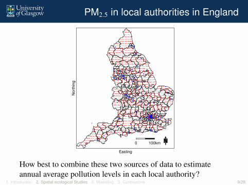
PM2.5 in local authorities in England

Easting

Nort

hin

g

0 100km

How best to combine these two sources of data to estimateannual average pollution levels in each local authority?


A common statistical model for these data

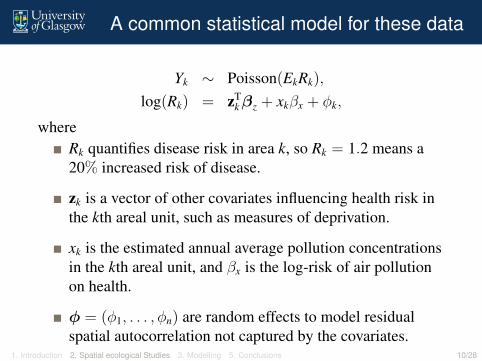
Yk ∼ Poisson(EkRk),

log(Rk) = zTkβz + xkβx + φk,

whereRk quantifies disease risk in area k, so Rk = 1.2 means a20% increased risk of disease.

zk is a vector of other covariates influencing health risk inthe kth areal unit, such as measures of deprivation.

xk is the estimated annual average pollution concentrationsin the kth areal unit, and βx is the log-risk of air pollutionon health.

φ = (φ1, . . . , φn) are random effects to model residualspatial autocorrelation not captured by the covariates.


Residual spatial autocorrelation

Spatial autocorrelation occurs when observationsgeographically close are more similar than those furtherapart.

The residuals from fitting a regression model to the healthdata with just (zT

k , xk) are typically spatially autocorrelated,requiring the random effect φk to account for it.

The autocorrelation is typically caused by unmeasuredconfounding, namely the presence of important spatiallysmooth risk factors that have been omitted from theregression model.

Ignoring this autocorrelation is known to bias βx.


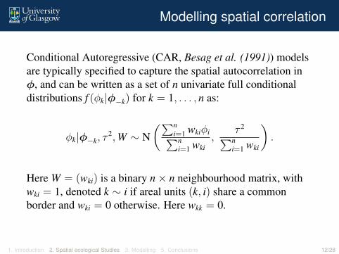
Modelling spatial correlation

Conditional Autoregressive (CAR, Besag et al. (1991)) modelsare typically specified to capture the spatial autocorrelation inφ, and can be written as a set of n univariate full conditionaldistributions f (φk|φ−k) for k = 1, . . . , n as:

φk|φ−k, τ2,W ∼ N

(∑ni=1 wkiφi∑n

i=1 wki,

τ 2∑ni=1 wki

).

Here W = (wki) is a binary n× n neighbourhood matrix, withwki = 1, denoted k ∼ i if areal units (k, i) share a commonborder and wki = 0 otherwise. Here wkk = 0.


Interpreting βx

The relative risk for a 1µgm−3 increase in pollutionconcentrations measures the proportional increase in health riskfrom increasing pollution by 1µgm−3, and is calculated as

RR(βx, 1) =Ek exp(zT

k βz + (xk + 1)βx + φk)

Ek exp(zTk βz + xkβx + φk)

= exp(1× βx).

Hence a relative risk of 1.03 means a 3% increase in diseaserisk when the pollution level increases by 1µgm−3.


Limitations - spatial autocorrelation

The CAR prior forces the random effects (φ1, . . . , φn) to beglobally spatially smooth everywhere. This causes twoproblems:

Collinearity with covariates that are also globally smoothsuch as air pollution, as was illustrated by Clayton et al.(1993) and Hughes and Haran (2013).

The spatial autocorrelation in the data remaining afteraccounting for the covariates is unlikely to be globallyspatially smooth, because the disease data (e.g. the SIR)are not globally smooth so the residuals after removingcovariate effects are also unlikely to be.

Both these may result in biased estimates of βx.


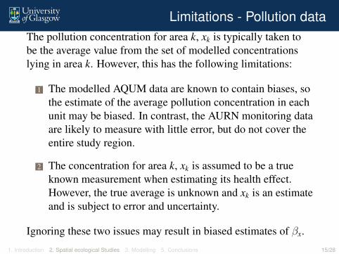
Limitations - Pollution dataThe pollution concentration for area k, xk is typically taken tobe the average value from the set of modelled concentrationslying in area k. However, this has the following limitations:

1 The modelled AQUM data are known to contain biases, sothe estimate of the average pollution concentration in eachunit may be biased. In contrast, the AURN monitoring dataare likely to measure with little error, but do not cover theentire study region.

2 The concentration for area k, xk is assumed to be a trueknown measurement when estimating its health effect.However, the true average is unknown and xk is an estimateand is subject to error and uncertainty.

Ignoring these two issues may result in biased estimates of βx.


3. Modelling

This project aims to address all of these statisticalshortcomings, by:

1 Developing a spatial regression model linking themonitoring and modelled pollution data, thus allowingaverage pollution concentrations xk to be predicted foreach areal unit with an associated measure of uncertainty.

2 Extending the health model so that it allows for theuncertainty in xk.

3 Extending the health model so that it models the spatialautocorrelation (a prior for (φ1, . . . , φn)) more flexibly thanthe global CAR model, allowing for local rather thanglobal patterns of spatial structure.


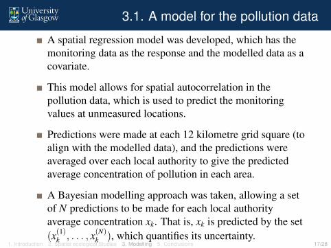
3.1. A model for the pollution data

A spatial regression model was developed, which has themonitoring data as the response and the modelled data as acovariate.

This model allows for spatial autocorrelation in thepollution data, which is used to predict the monitoringvalues at unmeasured locations.

Predictions were made at each 12 kilometre grid square (toalign with the modelled data), and the predictions wereaveraged over each local authority to give the predictedaverage concentration of pollution in each area.

A Bayesian modelling approach was taken, allowing a setof N predictions to be made for each local authorityaverage concentration xk. That is, xk is predicted by the set(x(1)k , . . . , x(N)

k ), which quantifies its uncertainty.1. Introduction 2. Spatial ecological Studies 3. Modelling 5. Conclusions 17/28

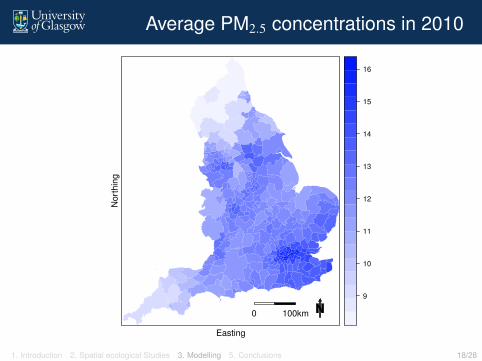
Average PM2.5 concentrations in 2010

Easting

Nort

hin

g

0 100km

9

10

11

12

13

14

15

16


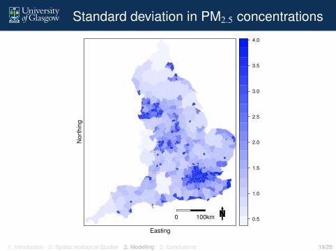
Standard deviation in PM2.5 concentrations

Easting

Nort

hin

g

0 100km 0.5

1.0

1.5

2.0

2.5

3.0

3.5

4.0


3.2. Allowing for uncertainty in xk

The standard regression model assumes xk is a known valuemeasured without error, which is unrealistic in this setting. Twomain statistical approaches have been proposed for correctingthis.

1 Measurement error models - This approach assumes thepredicted values (x(1)k , . . . , x(N)

k ) are error pronemeasurements of the single true but unknownconcentration xk.

2 Ecological bias models - This approach assumes thepredicted values (x(1)k , . . . , x(N)

k ) represent the range ofconcentrations in area k, allowing for within area variationin the concentrations.


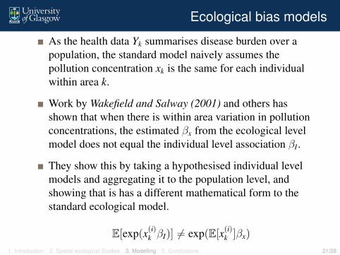
Ecological bias models

As the health data Yk summarises disease burden over apopulation, the standard model naively assumes thepollution concentration xk is the same for each individualwithin area k.

Work by Wakefield and Salway (2001) and others hasshown that when there is within area variation in pollutionconcentrations, the estimated βx from the ecological levelmodel does not equal the individual level association βI .

They show this by taking a hypothesised individual levelmodels and aggregating it to the population level, andshowing that is has a different mathematical form to thestandard ecological model.

E[exp(x(i)k βI)] 6= exp(E[x(i)k ]βx)


A model for ecological bias

Richardson et al (1987) show that one solution to overcome thisproblem is to change the model for Rk from

Rk = exp(zTk βz + µkβx + φk),

to

Rk = exp(zTk βz + µkβx + σ2

kβ2x/2 + φk),

thus explicitly incorporating the variation in xk. Here (µk, σ2k )

respectively denote the mean and variance of (x(1)k , . . . , x(N)k ).

This change is based on assuming the within area exposuredistribution is Gaussian, and comes direct from the momentgenerating function E[exp(x(i)k βI)].


The impact of ecological bias

The difference between the naive ecological model and thecorrected model is the term σ2

kβ2x/2, which is likely to be small

if:

βx is small.σ2

k is small.

The former is likely to be true and the latter may or may not be,and preliminary analyses show that the impact of ecologicalbias may be small for these studies.

We are currently investigating the exact extent of this problem.


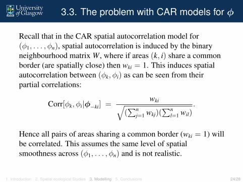
3.3. The problem with CAR models for φ

Recall that in the CAR spatial autocorrelation model for(φ1, . . . , φn), spatial autocorrelation is induced by the binaryneighbourhood matrix W, where if areas (k, i) share a commonborder (are spatially close) then wki = 1. This induces spatialautocorrelation between (φk, φi) as can be seen from theirpartial correlations:

Corr[φk, φi|φ−ki] =wki√

(∑n

j=1 wkj)(∑n

l=1 wil).

Hence all pairs of areas sharing a common border (wki = 1) willbe correlated. This assumes the same level of spatialsmoothness across (φ1, . . . , φn) and is not realistic.


Alternatives?

Ignore the spatial autocorrelation entirely and let φk = 0for all areas k.

Replace the random effects (φ1, . . . , φn) with an alternativespatial smoothing component that is forced to beorthogonal (unrelated) to the air pollution covariate, so thatspatial confounding cannot occur. Such an approach wasproposed by Hughes and Haran in (2013).

Extend the CAR model to make it more flexible and allowfor localised smoothness in the random effects, so thatgeographically adjacent values can be modelled as similaror very different.


Locally smooth CAR models

A number of approaches have been proposed to extend thestandard CAR model to allow for localised spatial smoothness.They can be broken into two main approaches:

Treat each wki relating to neighbouring areas as binaryrandom quantities, so that if wki is estimated as one then(φk, φi) are spatially smoothed, while if wki is estimated aszero they are not. Examples include Lee and Mitchell(2013) and Lee, Rushworth and Sahu (2014).

Augment the spatially smooth random effects with apiecewise constant jump component with different meanlevels, so that if two areas close together have differentmean levels their residuals will not be similar. Examplesinclude Lawson and Clark (2002), Lee et al (2014).


Results

The choice of residual spatial autocorrelation model can make alarge difference on the estimated pollution-health relationship.The estimated relative risks and 95% uncertainty intervals for a1µgm−3 increase in PM2.5 were:

Ignore correlation - 1.032 (1.005, 1.060).CAR model - 1.065 (1.043, 1.091).Orthogonal model - 1042 (1.040, 1.043).Localised CAR model - 1.046 (1.033, 1.060).

Both the estimates and uncertainty intervals can differsubstantially.


5. Conclusions

1 Developing a statistically valid approach for estimating thehealth effects of air pollution using spatial ecological datais a challenging task, and requires complex models forboth the pollution and health data.

2 Using an inappropriate statistical model results inestimated health effects that are likely to be biased.

3 Future work will extend this model into thespatio-temporal domain, and the replication of the spatialdata over time will enable more precise estimation of theair pollution effects.

4 The effects of air pollution will be investigated acrossScotland, to see if the England results are replicated here.


estimating the long-term health impact of air pollution using spatial ecological studies · ·...

Documents