1

RIETI Discussion Paper Series 15-E-00X *** 2015

Estimating the Impacts of FTA on Foreign Trade: An Analysis of Extensive and Intensive Trade Margins for Japan-Mexico FTA*

Arata Kuno†, Shujiro Urata‡, and Kazuhiko Yokota§

Abstract

This paper examines the impacts of Japan-Mexico FTA (JMXFTA), which was

enacted in 2005, on Japanese exports to Mexico. The authors construct a theoretical

trade model of heterogeneous firms, which is based on the Melitz-Chaney model, and

derive the theoretical relationship of the impacts of tariff changes on extensive and

intensive trade margins. Applying this model, the authors estimate the impacts of

JMXFTA on product-level extensive and intensive margins of Japan’s exports to

Mexico by using the most detailed commodity trade data. The results show that the

tariff reduction caused by JMXFTA increases intensive margin while no clear

evidence is found about the effect on extensive margin. This indicates that in the

short-run, the JMXFTA exerted more favorable effect on existing exporters than on

new export market entrants.

Key words: Free trade agreements, Extensive and intensive trade margins, Tariffs

JEL classification: F14, F15

* This study is conducted as a part of the Project “Economic Analysis on Trade Agreements” undertaken at Research Institute of Economy, Trade and Industry (RIETI). The author would like to thank RIETI for the fruitful research opportunity, Mitsuyo Ando, Hikaru Ishido, Kennichi Kawasaki, Fukunari Kimura, Eiichi Tomiura, and Ryuhei Wakasugi for helpful comments, and Youngmin Baek for efficient research assistance. In addition, we would like to thank the participants of the 5th Spring Meeting of the Japan Society of International Economics. The views expressed in this paper are the sole responsibility of the author. All remaining errors are our own. † Associate Professor, Faculty of Social Sciences, Kyorin University. Contact address: 476 Miyashita-cho, Hachioji, Tokyo 192-8508, Japan. E-mail: arata.kuno@gmail.com. ‡ Faculty fellow, RIETI and Professor, Graduate School of Asia-Pacific Studies, Waseda University. Contact address: 1-21-1 Nishiwaseda, Shinjuku-ward, Tokyo 169-0051, Japan. E-mail: surata@waseda.jp § Professor, School of Commerce, Waseda University. Contact address: 1-6-1 Nishiwaseda, Shinjuku-ward, Tokyo 169-8050, Japan. E-mail: yokota21@gmail.com.

RIETI Discussion Papers Series aims at widely disseminating research results in the form of professional

papers, thereby stimulating lively discussion. The views expressed in the papers are solely those of the

author(s), and do not represent those of the Research Institute of Economy, Trade and Industry.

2

1. Introduction

Japan has become active in establishing free trade agreements (FTAs) since the turn of the

century. The first FTA for Japan was with Singapore, which became effective in November 2002.

The second FTA was with Mexico, which became into action in April 2005. As of January 2014,

Japan has enacted 13 FTAs and signed one FTA awaiting ratification. The main objective of FTAs

for Japan is to expand exports to the FTA partners.

Since multilateral negotiations for trade liberalization under the General Agreement on

Tariffs and Trade (GATT)/World Trade Organization (WTO) became stalled, increasing number of

countries became interested in FTAs as a means to expand their exports, which would contribute to

economic growth. It was in the early 1990s when the Uruguay Round of multilateral trade

negotiations under the GATT were in deadlock that many countries began negotiating FTAs. The

FTA frenzy continued even after the WTO was established in 1995 and after the first multilateral

trade negotiations under the WTO, or the Doha Development Agenda (DDA), began in 2001,

because DDA negotiations were making no progress due to the differences in the opinions of the

WTO members on the DDA. Faced with increasing number of FTAs, which are discriminatory in the

sense that FTA members benefit from preferential access to FTA members’ market while non-FTA

members suffer from discrimination in those markets, Japan became interested in FTAs in order to

avoid discriminatory treatment in many countries in the world.

In light of increasing importance of FTAs for Japan’s trade policy, this paper attempts to

examine the impacts of Japan-Mexico FTA on Japan’s exports to Mexico. This type of research is

very important as it tries to confirm the expected impacts of FTAs. It is well known that FTAs would

lead to an expansion of trade between FTA partners, or the trade creation effect of an FTA. Ando and

Urata (2011) conducted a detailed analysis of the impacts of Japan-Mexico FTA (JMXFTA) on

bilateral trade and found that bilateral trade of many products, which were protected but liberalized

under the FTA, increased substantially1. This paper attempts to investigate the impacts of FTAs on

trade from different perspectives, that is, extensive and intensive margins, in order to deepen our

understanding of the issue by shedding new light2.

Not so long ago, we took for granted that trade liberalization expands trade volumes and in

turn leads to economic growth. However, since the last decade, some empirical as well as theoretical

researches have shed light on the fact that trade liberalization affects trade margins in two different

1 In their analysis of trade and regional trade agreements including FTAs and customs unions involving 67 countries for 27 years from 1980 to 2006, Urata and Okabe (2014) found positive or trade creation effect in many cases but not in all the cases. The presence of non-tariff barriers and/or difficulty in the use of FTAs seems to prevent the trade creation effect. 2 Unless otherwise specified, the terms “extensive margin” and “intensive margin” refer to the product-level margins rather than the partner-level margins.

3

ways. A change in trade margin can be decomposed into two margins, the change in trade volume

per existing traded good and the change in the number of traded goods. The former is referred to as

the intensive margin and the latter as the extensive margin. The intensive margin brought out by

trade liberalization simply means increasing production of a good that already has a comparative

advantage while decreasing the production of a good with comparative disadvantage. On the other

hand, the extensive margin indicates that the exporter starts to gain a comparative advantage in a

new good. In other words, the exporter who expands its trade volume through the extensive margin

experiences a change in production as well as trade structure. In this sense the effect caused by this

change may be long-lasting.3

Although the impact of these two margins on economic growth is still being investigated,

it is now widely recognized that distinguishing these margins is important when the effects of trade

liberalization are considered. In particular the extensive margin has been paid little attention as a

factor of trade expansion. The structure of the paper is as follows. Section 2 reviews the literature on

the impacts of FTAs and trade liberalization on intensive and extensive trade margins. Section 3

presents the model used for our analysis of the impacts of the JMXFTA on extensive and intensive

trade margins regarding Japan’s exports to Mexico. Our model is based on Melitz-Chaney type

heterogeneous firm trade, but it differs from their models in some points: our model addresses the

different characteristics by sector, and our model incorporates transport costs and tariff barriers

separately. This separation is important when we analyze the effect of tariff reduction. Section 4

provides an overall picture of Japan’s exports to Mexico before and after the FTA. Section 5

provides the details of the data of tariffs and exports. Section 6 presents and discusses the results of

the empirical analysis, and section 7 concludes the paper.

2. The Impacts of Trade Liberalization on Intensive and Extensive Trade Margins: Previous

Studies

Let us begin with theoretical explanation of the importance of considering the extensive

margins in the analysis of trade flows. Using heterogeneous firm framework, Chaney (2008)

examines the importance of the elasticity of substitution between goods in determining the effect of

trade barriers on export volumes, and shows that the magnitude of the elasticity of substitution

affects export volume through the intensive and extensive margins differently. Helpman, Melitz and

Rubinstein (2008) (hereafter HMR) argue the importance of the extensive margin in different way

from Chaney. They theoretically and empirically show that the estimates in gravity equation would

be biased if the extensive margin is omitted.

The question which margin is more affected by the trade liberalization is solely an

empirical issue. Using more than 5,000 product categories, Hummels and Klenow (2005) identify

3 Buono and Lalanne (2012) touch on this point.

4

that larger economies tend to export more than smaller economies and the extensive margin plays a

crucial role of their export expansion. Also adopting the Feenstra methodology, Kehoe and Ruhl

(2013) find that extensive margin contributed significantly to trade expansion between the US and its

FTA countries. Dutt, Mihov, and van Zandt (2013) focus on the impact of WTO membership on the

intensive and the extensive margins and find that the WTO membership raises the extensive margin

but decreases intensive margin with country-level data in the panel gravity model. There are some

other studies that show the significant impact of FTA on the extensive margin including Hillberry

and McDaniel (2002) on the impacts of the North American Free Trade Agreement (NAFTA) on the

NAFTA members’ trade and Foster (2012) on the effects of preferential trade agreements (PTAs) on

imports.4 These studies seem to indicate that the extensive margin plays an important role in

determining the size of trade in the case of policy change, as argued by Kehoe and Ruhl.

As seen from the discussions above, majority of the studies which we reviewed find that

trade liberalization and FTAs lead to an expansion of extensive margins of trade. However, there are

some studies, a few though, which find limited role of the extensive margin. Buono and Lalanne

(2012) estimate the impact of the Uruguay round on French firms’ export activities and find the tariff

reduction resulted in noticeable export expansion, mainly through the expansion of intensive margins.

This study uses firm-level data, unlike most other studies, which use trade data. Debaere and

Mostashari (2010) analyze the sources of the changes in the extensive margins of the exports to the

US by using disaggregated trade and tariff data, and find that tariff reduction has a limited impact on

the extensive margin.

3. The Model

In this section we set up a model which is used for the empirical study in a later section.

Our model has a similar structure to Chaney (2008) which theoretically incorporates intensive and

extensive margins into heterogeneous firm model a la Melitz (2003). We assume that consumers of a

country 𝑖𝑖 has the following utility function,

𝑈𝑈𝑖𝑖 = 𝑞𝑞0𝜇𝜇0�� � 𝑞𝑞𝑠𝑠

𝜔𝜔∈𝛺𝛺𝑠𝑠

(𝜔𝜔)𝜎𝜎𝑠𝑠−1𝜎𝜎𝑠𝑠 𝑑𝑑𝜔𝜔�

𝜇𝜇𝑠𝑠𝜎𝜎𝑠𝑠

𝜎𝜎𝑠𝑠−1𝑆𝑆

𝑠𝑠=1

.

There are S industries, and a representative consumer in the country 𝑖𝑖 consumes a homogeneous

4 There are some studies which have different definition of extensive margin, such as Fellbermyr and Kohler (2006) and Evenett and Venables (2002). They define the extensive margin is the number of new market (country) although Evenett and Venables don’t use the term “extensive”. In addition, Amurgo and Pierola (2008) develop the method to separate two extensive margins (the numbers of new products and new markets).

5

good, 𝑞𝑞0, and a continuum of differentiated goods 𝑞𝑞𝑠𝑠�ω�, ω ∈ 𝛺𝛺𝜔𝜔. The homogeneous good is assumed numeraire and freely traded between countries without any cost. The consumers spend a

share μ for each good, such that 𝜇𝜇0 + ∑ 𝜇𝜇𝑠𝑠𝑆𝑆𝑠𝑠=1 = 1. 𝜎𝜎𝑠𝑠 is the elasticity of substitution between

differentiated goods for sector s, and assumed 𝜎𝜎𝑠𝑠 − 1 > 0.

Maximizing the utility subject to the budget constraint gives the country 𝑖𝑖′s demand for differentiated goods of sector s.

𝑞𝑞𝑠𝑠𝑖𝑖(𝜔𝜔) = 𝜇𝜇𝑠𝑠𝑌𝑌𝑖𝑖𝑝𝑝𝑠𝑠𝑖𝑖(𝜔𝜔)−𝜎𝜎𝑠𝑠𝑃𝑃𝑠𝑠𝑖𝑖 . (1)

𝑌𝑌𝑖𝑖 is country 𝑖𝑖′s income and 𝜇𝜇𝑠𝑠𝑌𝑌𝑖𝑖 is the expenditure for the goods in sector s. 𝑃𝑃𝑠𝑠𝑖𝑖 is country

𝑖𝑖′s composite price index in sector s, given by

𝑃𝑃𝑠𝑠𝑖𝑖 = � � 𝑝𝑝𝑠𝑠𝑖𝑖𝜔𝜔∈𝛺𝛺𝑠𝑠

(𝜔𝜔)1−𝜎𝜎𝑠𝑠𝑑𝑑𝜔𝜔�

1𝜎𝜎𝑠𝑠−1

.

A firm in the country 𝑖𝑖 exports differentiated product to country 𝑗𝑗 covering

transportation costs and import tariff incurred by country 𝑗𝑗. The transportation costs include freight

and insurance which become greater as the distance between countries 𝑖𝑖 and 𝑗𝑗 becomes longer. We

assume that the cost is in the form of iceberg that country 𝑗𝑗 receives one unit of a good in sector s if country 𝑖𝑖 ships 𝜏𝜏𝑠𝑠𝑖𝑖𝑠𝑠 unit to country 𝑗𝑗. A tariff rate 𝑡𝑡𝑠𝑠𝑠𝑠 is incurred by country 𝑗𝑗 for sector s. We

assume that 𝜏𝜏𝑠𝑠𝑖𝑖𝑠𝑠 > 1 for 𝑖𝑖 ≠ 𝑗𝑗, and 𝜏𝜏𝑠𝑠𝑖𝑖𝑖𝑖 = 1, and 𝑡𝑡𝑠𝑠𝑠𝑠 > 0. There is an additional cost, 𝑓𝑓𝑠𝑠𝑖𝑖𝑠𝑠 , which

must be borne by a firm when it exports,5 given by 𝑓𝑓𝑠𝑠𝑖𝑖𝑠𝑠 > 0 for 𝑖𝑖 ≠ 𝑗𝑗, and 𝑓𝑓𝑠𝑠𝑖𝑖𝑖𝑖 = 0.

Assuming only labor is a factor of production, and the good 𝑞𝑞0 is produced under

constant returns to scale technology, while the differentiated products 𝑞𝑞𝑠𝑠(𝜔𝜔), 𝑠𝑠 > 1 are produced

under increasing returns to scale technology. Consider the case that a representative firm in country

𝑖𝑖 exports a differentiated good to country 𝑗𝑗. Maximizing the profit subject to the budget constraint,

we have the following optimal pricing rule which shows a constant mark-up over the marginal cost:

𝑝𝑝𝑠𝑠𝑖𝑖𝑠𝑠(𝜑𝜑) = 𝛼𝛼𝑤𝑤𝑖𝑖𝜏𝜏𝑠𝑠𝑖𝑖𝑠𝑠(1 + 𝑡𝑡𝑠𝑠𝑠𝑠)

𝜑𝜑, (2)

where 𝜑𝜑 is the firm’s labor productivity, 𝑤𝑤𝑖𝑖 is country 𝑖𝑖′𝑠𝑠 wage rate which equals to the

5 To keep the model as simple as possible, we assume there is no fixed cost for entering the market. In other words, the firm has two choices, supplies to domestic market or supplies to both domestic market and country 𝑗𝑗.

6

marginal cost, and 𝛼𝛼 = 𝜎𝜎𝑠𝑠 (𝜎𝜎𝑠𝑠 − 1)⁄ . As in HMR (2008), Chaney (2008), and others, we assume the

productivity 𝜑𝜑 follows Pareto distribution over the range of [1, +∞);

Pr(𝜑𝜑� < 𝜑𝜑) = 𝐺𝐺(𝜑𝜑) = 1 − 𝜑𝜑−𝛾𝛾𝑠𝑠 ,

where parameter 𝛾𝛾𝑠𝑠 stands for the curvature of the density with 𝛾𝛾𝑠𝑠 > 𝜎𝜎𝑠𝑠 − 1. Using equations (1)

and (2), we have the demand for differentiated goods produced in country 𝑖𝑖 and sold in country 𝑗𝑗

of sector s as follows:

𝑥𝑥𝑠𝑠𝑖𝑖𝑠𝑠(𝜑𝜑) = 𝑝𝑝𝑠𝑠𝑠𝑠(𝜑𝜑)𝑞𝑞𝑠𝑠𝑖𝑖𝑠𝑠(𝜑𝜑) = 𝜇𝜇𝑠𝑠𝑌𝑌𝑠𝑠𝛼𝛼1−𝜎𝜎𝑠𝑠 �𝑤𝑤𝑖𝑖�1 + 𝑡𝑡𝑠𝑠𝑠𝑠�𝜏𝜏𝑠𝑠𝑖𝑖𝑠𝑠

𝜑𝜑�1−𝜎𝜎𝑠𝑠

𝑃𝑃𝑠𝑠𝑠𝑠𝜎𝜎𝑠𝑠−1. (3)

We next consider the heterogeneity of producers. To find the volume of differentiated

goods exports from country 𝑖𝑖 to country j in the heterogeneous firm model, we define the

productivity threshold using the density function above. Since the firm’s profit in the country 𝑖𝑖

from exporting differentiated goods to country 𝑗𝑗 is 𝜋𝜋𝑠𝑠𝑖𝑖𝑠𝑠(𝜑𝜑) = �𝑝𝑝𝑠𝑠𝑠𝑠(𝜑𝜑)− 𝑤𝑤𝑖𝑖�1+𝑡𝑡𝑠𝑠𝑠𝑠�𝜏𝜏𝑠𝑠𝑖𝑖𝑠𝑠𝜑𝜑

� 𝑞𝑞𝑠𝑠𝑖𝑖𝑠𝑠(𝜑𝜑)−

𝑓𝑓𝑠𝑠𝑖𝑖𝑠𝑠, the threshold is obtained to solve for 𝜑𝜑 by setting 𝜋𝜋𝑠𝑠𝑖𝑖𝑠𝑠(𝜑𝜑) = 0. We therefore obtain,

𝜑𝜑� = 𝛼𝛼𝛼𝛼 �𝑓𝑓𝑠𝑠𝑖𝑖𝑠𝑠𝜇𝜇𝑠𝑠𝑌𝑌𝑠𝑠

�

1𝜎𝜎𝑠𝑠−1 𝑤𝑤𝑖𝑖�1 + 𝑡𝑡𝑠𝑠𝑠𝑠�𝜏𝜏𝑠𝑠𝑖𝑖𝑠𝑠

𝑃𝑃𝑠𝑠𝑠𝑠. (4)

Equation (4) indicates that an increase in either export fixed cost (𝑓𝑓𝑠𝑠𝑖𝑖𝑠𝑠), marginal cost (𝑤𝑤𝑖𝑖),

tariff rate (𝑡𝑡𝑠𝑠𝑠𝑠), or transportation cost (𝜏𝜏𝑠𝑠𝑖𝑖𝑠𝑠) increase the threshold of export (𝜑𝜑�). On the other hand,

an increase in either demand share (𝜇𝜇𝑠𝑠), income (𝑌𝑌𝑠𝑠), or price index (𝑃𝑃𝑠𝑠𝑠𝑠) reduces 𝜑𝜑�.

With this result, we calculate the number of exported goods which equals the number of

exporters. Combining the maximum number of differentiated goods with Pareto distribution, we

have the following:

𝐸𝐸𝑠𝑠𝑖𝑖𝑠𝑠 = � 𝑁𝑁𝑠𝑠𝑖𝑖𝑑𝑑𝐺𝐺(𝜑𝜑) = 𝑁𝑁𝑠𝑠𝑖𝑖𝜑𝜑�−𝛾𝛾𝑠𝑠∞

𝜑𝜑�

, (5)

where 𝐸𝐸𝑠𝑠𝑖𝑖𝑠𝑠 is the number of goods exported from country 𝑖𝑖 to country j, and 𝑁𝑁𝑠𝑠𝑖𝑖 is the maximum

number of differentiated goods produced in sector s in country j. Equations (4) and (5) indicate that 𝐸𝐸𝑠𝑠𝑖𝑖𝑠𝑠 is a function of the maximum number of differentiated goods in sector s, the entry cost into

7

export market, sector-wise income of country j, marginal cost, transportation costs, price index, and the tariff rate. Among these variables, an increase in either 𝑓𝑓𝑠𝑠𝑖𝑖𝑠𝑠, 𝑤𝑤𝑖𝑖, 𝑡𝑡𝑠𝑠𝑠𝑠, or 𝜏𝜏𝑠𝑠𝑖𝑖𝑠𝑠 decrease 𝐸𝐸𝑠𝑠𝑖𝑖𝑠𝑠, by

raising 𝜑𝜑�. On the other hand, an increase in variables such as 𝜇𝜇𝑠𝑠, 𝑌𝑌𝑠𝑠, or 𝑃𝑃𝑠𝑠𝑠𝑠 raises 𝐸𝐸𝑠𝑠𝑖𝑖𝑠𝑠 through the

reduction in 𝜑𝜑�.

The extensive margin, we define, is a change in the number of exported differentiated

goods by sector. In order to obtain the extensive margin of exports, we take logarithm and deference

in terms of time of both side of equation (5).

On the other hand, the intensive margin of export is defined as a change in the average

volume of exported differentiated goods by sector. To see this, we first calculate the total volume of

trade in differentiated goods. This volume of exports 6 is calculated from the number of

differentiated goods 𝑁𝑁𝑠𝑠𝑖𝑖 and the volume of exported goods for sector s which is described by

equation (3). Then we have7

𝑋𝑋𝑠𝑠𝑖𝑖𝑠𝑠 = � 𝑁𝑁𝑠𝑠𝑖𝑖𝑥𝑥𝑠𝑠𝑖𝑖𝑠𝑠(𝜑𝜑)𝑑𝑑𝐺𝐺(𝜑𝜑)

∞

𝜑𝜑�

= 𝜇𝜇𝑠𝑠𝑌𝑌𝑠𝑠 �𝛼𝛼𝑤𝑤𝑖𝑖�1 + 𝑡𝑡𝑠𝑠𝑠𝑠�𝜏𝜏𝑠𝑠𝑖𝑖𝑠𝑠

𝑃𝑃𝑠𝑠𝑠𝑠�1−𝜎𝜎𝑠𝑠 𝛾𝛾𝑠𝑠

𝛾𝛾𝑠𝑠 − (𝜎𝜎𝑠𝑠 − 1)𝜑𝜑�𝜎𝜎𝑠𝑠−1𝑁𝑁𝑠𝑠𝑖𝑖𝜑𝜑�−𝛾𝛾𝑠𝑠 .

(6)

The term, 𝑁𝑁𝑠𝑠𝑖𝑖𝜑𝜑�−𝛾𝛾𝑠𝑠, is the number of exports in differentiated goods defined by equation (5), and the

𝜑𝜑� is a threshold condition which is defined by equation (4).

The total volume of differentiated good exports can be divided into two parts: the number of exported differentiated goods and the average volume of the differentiated exports, or 𝑋𝑋𝑠𝑠𝑖𝑖𝑠𝑠 =

𝐸𝐸𝑠𝑠𝑖𝑖𝑠𝑠 × �𝑋𝑋𝑠𝑠𝑖𝑖𝑠𝑠/𝐸𝐸𝑠𝑠𝑖𝑖𝑠𝑠�. 𝐸𝐸𝑠𝑠𝑖𝑖𝑠𝑠 is shown in equation (5), while the term �𝑋𝑋𝑠𝑠𝑖𝑖𝑠𝑠/𝐸𝐸𝑠𝑠𝑖𝑖𝑠𝑠� can be shown as

follows:

𝐼𝐼𝑠𝑠𝑖𝑖𝑠𝑠 = 𝜇𝜇𝑠𝑠𝑌𝑌𝑠𝑠 �𝛼𝛼𝑤𝑤𝑖𝑖�1 + 𝑡𝑡𝑠𝑠𝑠𝑠�𝜏𝜏𝑠𝑠𝑖𝑖𝑠𝑠

𝑃𝑃𝑠𝑠𝑠𝑠�1−𝜎𝜎𝑠𝑠 𝛾𝛾𝑠𝑠

𝛾𝛾𝑠𝑠 − (𝜎𝜎𝑠𝑠 − 1)𝜑𝜑�𝜎𝜎𝑠𝑠−1 (7)

The extensive and the intensive margins are changes in volume of equations (5) and (7).

Taking natural logarithm and difference with respect to time of both sides of the equation, we have

∆ln𝑋𝑋𝑠𝑠𝑖𝑖𝑠𝑠 = ∆ln𝐸𝐸𝑠𝑠𝑖𝑖𝑠𝑠 + ∆ln� 𝑋𝑋𝑠𝑠𝑖𝑖𝑠𝑠/𝐸𝐸𝑠𝑠𝑖𝑖𝑠𝑠�. We define that the extensive margin is the first term and the

intensive margin is the second term of the right side of the equation.

6 The total volume of exports includes homogeneous good and differentiated goods. To make the model as simple as possible, we ignore the trade in homogeneous goods trade. 7 The model analyzes the export from country 𝑖𝑖 to country j, only national income of country j appears in the equation which differs from Chaney’s (2008) model.

8

Hence, from equation (7), the intensive margin of trade includes the entry cost into export

market, sector-wise income of country j, marginal cost, transportation costs, price index, the tariff

rate, and the threshold condition.

Impact of FTA on extensive and intensive margins

Next we analyze the effect of FTA on the intensive and the extensive margins. Let us first

define the effect of FTA is the same as a decrease in tariff rate of country 𝑗𝑗. First we analyze the

effect of FTA on the extensive margin. It is clear that from equations (4) and (5), the extensive

margin is a function of a tariff rate, and a decrease in tariff rate reduces the threshold point, 𝜑𝜑�, and in

turn a decrease in 𝜑𝜑� raises the extensive margin since −𝛾𝛾𝑠𝑠 < 0. We hereafter refer to this as a

productivity effect.

Now note that the country 𝑗𝑗′s income 𝑌𝑌𝑠𝑠 is also a function of tariff rate 𝑡𝑡𝑠𝑠𝑠𝑠 because 𝑌𝑌𝑠𝑠

is expressed by ∑ 𝑤𝑤𝑠𝑠𝑠𝑠𝐿𝐿𝑠𝑠𝑠𝑠=1 +∑ �∫ 𝜋𝜋𝑠𝑠𝑠𝑠𝑖𝑖(𝜑𝜑)∞

0 𝑑𝑑𝐺𝐺(𝜑𝜑) + ∫ 𝑡𝑡𝑠𝑠𝑠𝑠𝑞𝑞𝑠𝑠𝑖𝑖𝑠𝑠(𝜑𝜑)∞

𝜑𝜑� 𝑑𝑑𝐺𝐺(𝜑𝜑)�𝑠𝑠=1 . 8 The first term

(𝑤𝑤𝑠𝑠𝑠𝑠𝐿𝐿𝑠𝑠) means the total labor income of country 𝑗𝑗, the first integral in the bracket expresses sum of

firm’s profit, and the second integral in the bracket stands for collected tariff revenue. An increase in

tariff rate creates tariff revenue which tends to raise country 𝑗𝑗′s income, 𝑌𝑌𝑠𝑠 . Since ∂𝑌𝑌𝑠𝑠 𝜕𝜕𝑡𝑡𝑠𝑠𝑠𝑠⁄ > 0 from the equation of 𝑌𝑌𝑠𝑠 above, a decrease in 𝑡𝑡𝑠𝑠𝑠𝑠 reduces 𝑌𝑌𝑠𝑠 and in turn raises 𝜑𝜑�. This finally

reduces 𝐸𝐸𝑠𝑠𝑖𝑖𝑠𝑠. However, many researchers find the positive correlation between trade liberalization

and national income such as Sachs and Warner (1995), Krueger (1997), and Frankel and Romer

(1999), to name a few. If this is the case, the effect of the tariff reduction on the national income can

be positive. The total effect of the FTA on the national income is therefore ambiguous. We hereafter

refer to this as an indirect income effect.9 The combined effect of the formation of the FTA on the

extensive margin hence depends on the balance of strength between the two.

PROPOSITION 1: Extensive margin is positive if and only if the elasticity of income with respect to

the tariff is smaller than (𝜎𝜎𝑠𝑠 − 1). 𝜀𝜀𝑦𝑦𝑡𝑡 < (𝜎𝜎𝑠𝑠 − 1).

PROOF: Inserting equation (4) into equation (5) and taking natural logarithm of both sides of the

equation, and taking derivative with respect to ln�1 + 𝑡𝑡𝑠𝑠𝑠𝑠�, we have:

𝜕𝜕ln𝐸𝐸𝑠𝑠𝑖𝑖𝑠𝑠𝜕𝜕ln�1 + 𝑡𝑡𝑠𝑠𝑠𝑠�

= 𝛾𝛾𝑠𝑠 �1

𝜎𝜎𝑠𝑠 − 1𝜀𝜀𝑦𝑦𝑡𝑡 − 1�,

8 However 𝑃𝑃𝑠𝑠𝑠𝑠 is not a function of 𝑡𝑡𝑠𝑠𝑠𝑠. Since 𝑃𝑃𝑠𝑠𝑠𝑠 is a function of an optimum price of country j, (𝑝𝑝𝑠𝑠𝑠𝑠) which is a function of 𝑡𝑡𝑠𝑠𝑖𝑖. 9 Chaney (2008), Crozet and Koenig (2010), and Arkolakis (2010) assume the income effect is independent of policy changes, which is different from our model.

9

where 𝜀𝜀𝑦𝑦𝑡𝑡 = 𝜕𝜕ln𝑌𝑌𝑠𝑠 𝜕𝜕ln�1 + 𝑡𝑡𝑠𝑠𝑠𝑠�⁄ , which means the elasticity of tariff with respect to the national

income. If this equation is negative, the FTA expands the extensive margin of the trade. This is

positive if and only if 𝜀𝜀𝑦𝑦𝑡𝑡 < (𝜎𝜎𝑠𝑠 − 1). If this is the case, the FTA expands the extensive margin. ■

We next analyze the impact of FTA on the intensive margin. Since the intensive margin

can be obtained by differencing the average volume of each export, we focus on the relation between

the left and right sides of the equation (7). In the right side of equation (7), tariff rate appears four times: in the nominator in the parenthesis, 𝑌𝑌𝑠𝑠, and two times in 𝜑𝜑�. We name the effect of 𝑡𝑡𝑠𝑠𝑠𝑠 in the

nominator in the parenthesis and 𝑌𝑌𝑠𝑠 as direct effect and direct income effect, respectively. The

effects of 𝑡𝑡𝑠𝑠𝑠𝑠 through 𝜑𝜑� are referred as the productivity and the indirect income effects, same as in

the case of extensive margin. Taking care of the sign of the power of the parenthesis (𝜎𝜎𝑠𝑠 − 1 > 0), we derive the direct effect of tariff reduction: ∂ 𝐼𝐼𝑠𝑠𝑖𝑖𝑠𝑠 𝜕𝜕𝑡𝑡𝑠𝑠𝑠𝑠⁄ < 0. Hence the effect of forming FTA

increases the intensive margin. The direct income effect, on the other hand, shows the negative

correlation between the intensive margin and the direct income effect.

PROPOSITION 2: (A) Intensive margin is positive if and only if the elasticity of income with

respect to the tariff is smaller than (𝜎𝜎𝑠𝑠 − 1), that is 𝜀𝜀𝑦𝑦𝑡𝑡 < (𝜎𝜎𝑠𝑠 − 1), when the productivity effects

are ignored. (B) However if the productivity effect is included, the effect of tariff reduction on the

intensive margin becomes neutral.10

PROOF:

(A) Taking derivative of equation (7) without the productivity term (𝜑𝜑�𝜎𝜎𝑠𝑠−1), we have the following

result,

𝜕𝜕ln𝐼𝐼𝑠𝑠𝑖𝑖𝑠𝑠𝜕𝜕ln�1 + 𝑡𝑡𝑠𝑠𝑠𝑠�

= 𝜀𝜀𝑦𝑦𝑡𝑡 − (𝜎𝜎𝑠𝑠 − 1).

It should be negative if 𝜀𝜀𝑦𝑦𝑡𝑡 < (𝜎𝜎𝑠𝑠 − 1). If this is the case, the FTA expands the intensive margin.

(B) Taking derivative of equation (7) with the productivity term (𝜑𝜑�𝜎𝜎𝑠𝑠−1), we have the following

result,

𝜕𝜕ln𝐼𝐼𝑠𝑠𝑖𝑖𝑠𝑠𝜕𝜕ln�1 + 𝑡𝑡𝑠𝑠𝑠𝑠�

= 𝜀𝜀𝑦𝑦𝑡𝑡 + (1− 𝜎𝜎𝑠𝑠) + (𝜎𝜎𝑠𝑠 − 1) �−1

𝜎𝜎𝑠𝑠 − 1𝜀𝜀𝑦𝑦𝑡𝑡 + 1� = 0.

10 This result is similar to the effect of fixed cost on trade flows of Chaney (2008), p.1717.

10

■

It is easy to infer the impact of FTA on total exports 𝑋𝑋𝑠𝑠𝑖𝑖𝑠𝑠 from these propositions. For the

case without productivity effect, it becomes

�𝜀𝜀𝑦𝑦𝑡𝑡 − (𝜎𝜎𝑠𝑠 − 1)� �1 +𝛾𝛾𝑠𝑠

𝜎𝜎𝑠𝑠 − 1�,

which is positive or negative depending on the sign of 𝜀𝜀𝑦𝑦𝑡𝑡 − (𝜎𝜎𝑠𝑠 − 1). On the other hand, the effect

with productivity path is just the same as the effect on extensive margin in proposition 1.

4. Japan’s Exports to Mexico

Japan’s exports to Mexico began to increase sharply in 2003 after experiencing a slow

decline for several years (Figure 1). The rate of increase of Japan’s exports to Mexico from 2003 to

2007 was very high as the magnitude of the exports increased 2.7 fold in 4 years, to register 1.1

trillion yen in 2007. A major reason for the rapid expansion of Japan’s exports to Mexico is high

economic growth achieved by the Mexican economy, which registered 4~5 percent growth rates for

the 2003-2007 period. In addition, the Japan-Mexico Free Trade Agreement, which became effective

in March 2005, appears to have also contributed to the rapid expansion of Japan’s exports to Mexico.

Japan’s exports to Mexico dropped precipitously to 600 billion yen in 2009 as Mexico’s GDP

declined by 4.7 percent due to the negative impacts caused by the Global Financial Crisis in 2008.

Japan’s exports to Mexico recovered quickly in 2010, as the Mexican economy recovered quickly

and strongly. Japan’s exports to Mexico remained at around 800 billion yen from 2010 to 2013.

Japan’s exports to Mexico are concentrated in machinery products. Specifically, the

average shares of general, electric, and electronic machinery and transport machinery in Japan’s total

exports to Mexico for the 2000-2013 period were 44.4 and 28.6 percent, respectively. Other products

which recorded relatively high shares include base metals, precision machinery, and chemical

products and plastics, whose shares in total exports were 12.2, 6.9 and 4.9 percent, respectively. The

combined share of these five products in Japan’s total exports to Mexico was as high as 97 percent.

It should be noted that these shares remained more or less the same throughout the 2000-2013

period.

Let us turn to a detailed examination of the patterns of Japan’s exports to Mexico in terms

of extensive and intensive margins in 2004 and 2006, for which we conduct a statistical analysis, in

order to discern the impacts of the Japan-Mexico Free Trade Agreement on Japan’s exports to

Mexico. We selected the years 2004 and 2006 for our analysis because of the availability of the most

detailed export data on the consistent classification basis (HS-9 digit).

11

Table 1 summarizes Japan’s exports to Mexico in terms of yen value and the number of

products at HS-9 digit level. The total number of products that Japan exported to the world in 2004

and 2006 amounted to 6,150 (Table 1). The number of products that are exported to Mexico in 2004

(pre-JMXFTA) and 2006 (post-JMXFTA) were 1,841 (1,493+348) and 1,859 (1,493+366),

respectively. Interestingly, the total number of exported products from Japan to Mexico grew less

than one percent during the period, despite a significant tariff reduction under the JMXFTA.

On the contrary, the value of Japan’s total exports to Mexico increased 1.86-fold from 553

billion yen to 1,030 billion yen from 2004 to 2006 (Table 1). Of these, the value of the products that

were exported both in 2004 and 2006 increased 1.85-fold from 540 billion yen to 1,002 billion yen

(intensive margin). Whether this significant increase in Japanese export value was achieved by

Mexico’s tariff reduction under the JMXFTA is an empirical matter. The values of exports that were

exported only in 2004 and only in 2006 were 12 billion yen and 28 billion yen, respectively. These

values amount to meager 2.2 percent and 2.8 percent of the total export values for 2004 and 2006,

respectively, indicating that the turnaround (entry and exit from the export market) in Japan’s exports

to Mexico occurred mostly for the products whose export values are quite small. In other words,

exported products with large value tended to be exported in both years.

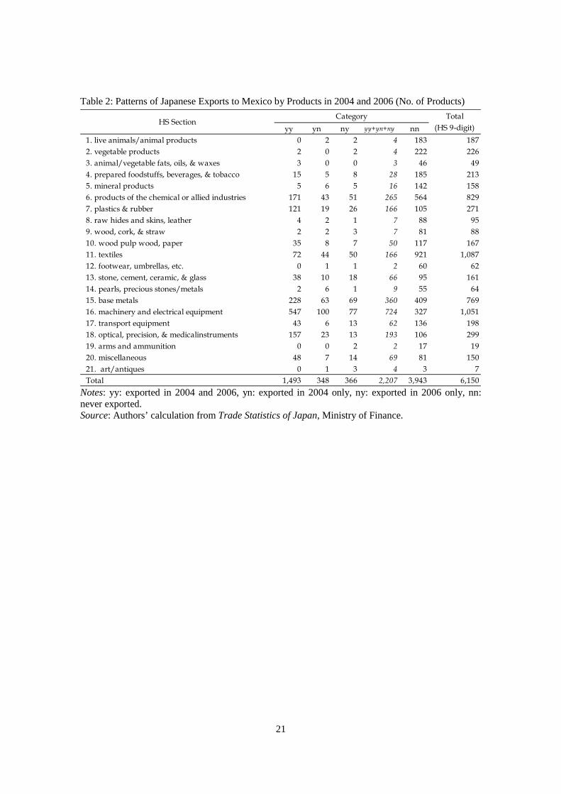
An examination of Japanese exports to Mexico by products reveals that the number of

products classified under general and electrical equipment is by far the largest, as the number of

products under these categories exported in 2004 and 2006 (for both years as well as just for one

year) amounted to 724, or 32.8 percent of the total number of exported products (Tables 2). Other

categories that registered a large number of exported products are base metals (360, 16.3%),

chemical products (265, 12.0%), precision machinery (193, 8.7%), plastics & rubber (166, 7.5%),

and textiles (166, 7.5%). These six industries as a group account for 84.9% of the total number of

products. These are the industries that experienced a substantial turnaround of the products in terms

of export status, i.e. exiting from as well as entering into the export market. Focusing on these six

industries, we find different patterns of change in the export status of the products. For general and

electric machinery, and precision machinery, the number of products exited from the export market

is larger than the number of products entered into the export market, resulting in the decline in the

number of exported products. By contrast, for base metals, chemical products, plastics & rubber, and

textiles, the number of products entering the export market was larger than the number of products

exiting from the export market, leading to an increase in the number of exported products. Besides

these four industries, stone, cement, ceramic & glass, and transport machinery saw an increase in the

number of exported products from 2004 to 2006.

The changing pattern of Japanese exports to Mexico in terms of export value shows quite a

different picture compared to the pattern observed in terms of product numbers (Table 3). As for the

products that were exported both in 2004 and 2006, a large increase in export value (intensive

12

margin) was observed in general and electric machinery (227 billion yen), and in transport

machinery (162 billion yen).11 In terms of growth rate, pearls, precious stones/metals recorded a

huge increase of 1,300 percent. Other than this industry, prepared foodstuffs, beverages & tobacco,

stone, cement, ceramic & glass, animal/vegetable fats, oils & waxes, and transport machinery

showed high increase of more than 200 percent. An investigation of the turnover of the exit from and

entry into the Mexican market by product shows that the value of newly exported products in

transport machinery in 2006 was large at 20 billion yen, accounting for as much as 70.5 percent of

the total value of newly exported products. For the transport machinery, the value of exported

products that exited from the export market was small at 300 million yen. The net increase resulting

from the turnover was quite large at 19.7 billion yen. The values of newly exported products were

quite large for base metals and general and electric machinery, respectively at 3.4 billion yen and 2.1

billion yen, but the values of the products exited from the exported market were significantly larger,

respectively at 5.0 billion yen and 4.9 billion yen, resulting in the net decline in the turnover value.

5. Empirical Analysis

5.1 Empirical Framework

We estimate the impact of FTA on trade flows, in particular extensive and intensive

margins by applying the model developed in section 3. Following HMR (2008), we assume 𝜏𝜏𝑠𝑠𝑖𝑖𝑠𝑠 = 𝑑𝑑𝑖𝑖𝑠𝑠𝑒𝑒𝑢𝑢𝑠𝑠, where 𝑑𝑑𝑖𝑖𝑠𝑠 represents physical distance between countries 𝑖𝑖 and 𝑗𝑗, and 𝑢𝑢𝑠𝑠 is the

error term with a mean of 0 and a variance of 𝜎𝜎2. In order to estimate of the effect of FTA on the

extensive margin, we insert equation (4) in equation (5) and then take logarithm of equations (5),

ln𝐸𝐸𝑠𝑠𝑖𝑖𝑠𝑠 = 𝛽𝛽𝐸𝐸 +𝛾𝛾𝑠𝑠

𝜎𝜎𝑠𝑠 − 1ln𝜇𝜇𝑠𝑠𝑌𝑌𝑠𝑠−𝛾𝛾𝑠𝑠ln�1 + 𝑡𝑡𝑠𝑠𝑠𝑠� −

𝛾𝛾𝑠𝑠𝜎𝜎𝑠𝑠 − 1

ln𝑓𝑓𝑠𝑠𝑖𝑖𝑠𝑠−𝛾𝛾𝑠𝑠ln𝑤𝑤s𝑖𝑖−𝛾𝛾𝑠𝑠ln𝑑𝑑𝑖𝑖𝑠𝑠 + 𝛾𝛾𝑠𝑠ln𝑃𝑃𝑠𝑠𝑠𝑠 + 𝑢𝑢𝑠𝑠,

where 𝛽𝛽𝐸𝐸 = ln𝑁𝑁𝑠𝑠 − 𝛾𝛾𝑠𝑠𝛼𝛼ln𝛼𝛼 which is constant over time. It is often observed that productivity

difference, strength of labor unions, inertia of mobility, and others lead to different wage rates over

industries. We assume, therefore, the marginal product of labor differs over sectors. The extensive

margin can be obtained by taking the difference in terms of time of the equation.

∆ln𝐸𝐸𝑠𝑠𝑖𝑖𝑠𝑠 = 𝛾𝛾𝑠𝑠𝜎𝜎𝑠𝑠−1

∆ln𝜇𝜇𝑠𝑠𝑌𝑌𝑠𝑠−𝛾𝛾𝑠𝑠∆ln�1 + 𝑡𝑡𝑠𝑠𝑠𝑠� −𝛾𝛾𝑠𝑠

𝜎𝜎𝑠𝑠−1∆ln𝑓𝑓𝑠𝑠𝑖𝑖𝑠𝑠−𝛾𝛾𝑠𝑠∆ln𝑤𝑤𝑠𝑠𝑖𝑖 + 𝛾𝛾𝑠𝑠∆ln𝑃𝑃𝑠𝑠𝑠𝑠 + ∆𝑢𝑢𝑠𝑠 . (8)

We apply the same procedure to equation (7) to get the estimated equation for the intensive margin

for the case of no-productivity path (assuming 𝜑𝜑� = 1).

11 It is worth noting that prior to the JMXFTA, automobile producers who did not have any production sites in Mexico had to bear 50 percent of import tax. See Ando and Urata (2011).

13

ln𝐼𝐼𝑠𝑠𝑖𝑖𝑠𝑠 = 𝛽𝛽𝐼𝐼 + ln𝜇𝜇𝑠𝑠𝑌𝑌𝑠𝑠 − (𝜎𝜎𝑠𝑠 − 1)�ln�1 + 𝑡𝑡𝑠𝑠𝑠𝑠�+ ln𝑓𝑓𝑠𝑠𝑖𝑖𝑠𝑠 + ln𝑤𝑤𝑠𝑠𝑖𝑖 + ln𝑑𝑑𝑖𝑖𝑠𝑠 − ln𝑃𝑃𝑠𝑠𝑠𝑠� + 𝑢𝑢𝑠𝑠,

where 𝛽𝛽𝐼𝐼 = ln 𝛾𝛾𝑠𝑠𝛾𝛾𝑠𝑠−(𝜎𝜎𝑠𝑠−1) − (𝜎𝜎𝑠𝑠 − 1)ln𝛼𝛼 which is constant over time. The intensive margin is

obtained from time-differencing the equation,

∆ln𝐼𝐼𝑠𝑠𝑖𝑖𝑠𝑠 = ∆ln𝜇𝜇𝑠𝑠𝑌𝑌𝑠𝑠 − (𝜎𝜎𝑠𝑠 − 1)�∆ln�1 + 𝑡𝑡𝑠𝑠𝑠𝑠�+ ∆ln𝑓𝑓𝑠𝑠𝑖𝑖𝑠𝑠 + ∆ln𝑤𝑤𝑠𝑠𝑖𝑖 − ∆ln𝑃𝑃𝑠𝑠𝑠𝑠� + ∆𝑢𝑢𝑠𝑠. (9)

Equations (8) and (9) are different from theoretical gravity equations developed by, for

example, Chaney (2008), Anderson and van Wincoop (2003), and HMR. (2008).12 The most important difference from them is the inclusion of the sector level income effect, ie., ∆ln𝜇𝜇𝑠𝑠𝑌𝑌𝑠𝑠. Since

we focus on the impact of FTA by sector, the term of sector specific demand plays an important role

although all previous studies ignore it.13 The second important difference is the presence of the policy variable 𝑡𝑡𝑠𝑠𝑠𝑠. We explicitly separate the policy variable of trade liberalization 𝑡𝑡𝑠𝑠𝑠𝑠 from the

transportation costs 𝜏𝜏𝑠𝑠𝑖𝑖𝑠𝑠. This separation is particularly important for a policy analysis because the

transportation costs 𝜏𝜏𝑠𝑠𝑖𝑖𝑠𝑠 contains a physical distance between the two countries which is not a

policy variable.

In the empirical analysis, country 𝑗𝑗’s imports from the world for the goods in sector 𝑠𝑠 (𝑀𝑀𝑠𝑠𝑠𝑠) are used as a proxy for the sector level expenditure for the goods in the sector (𝜇𝜇𝑠𝑠𝑌𝑌𝑠𝑠). The

utilization rate of FTA preferential tariffs is assumed to be 100%. In other words, exporters in

country 𝑖𝑖 always make use of preferential tariff rates granted by country 𝑗𝑗 whenever possible. We also assume that fixed cost in each sector (𝑓𝑓𝑠𝑠𝑖𝑖𝑠𝑠) and distance between countries 𝑖𝑖 and 𝑗𝑗 (𝑑𝑑𝑖𝑖𝑠𝑠) are

constant over time.

Consequently, the equations to be estimated are given by:

∆ln𝐸𝐸𝑠𝑠𝑖𝑖𝑠𝑠 = 𝛽𝛽1𝑒𝑒𝑒𝑒∆ ln𝑇𝑇𝑠𝑠𝑠𝑠 + 𝛽𝛽2𝑒𝑒𝑒𝑒∆ln𝑀𝑀𝑠𝑠𝑠𝑠 + 𝛽𝛽3𝑒𝑒𝑒𝑒∆ln𝑤𝑤𝑖𝑖𝑠𝑠 + 𝛽𝛽4𝑒𝑒𝑒𝑒∆ln𝑃𝑃𝑠𝑠𝑠𝑠 + 𝑢𝑢𝑠𝑠 , (8)′

∆ln𝐼𝐼𝑠𝑠𝑖𝑖𝑠𝑠 = 𝛽𝛽1𝑖𝑖𝑖𝑖∆ ln𝑇𝑇𝑠𝑠𝑠𝑠 + 𝛽𝛽2𝑖𝑖𝑖𝑖∆ln𝑀𝑀𝑠𝑠𝑠𝑠 + 𝛽𝛽3𝑖𝑖𝑖𝑖∆ln𝑤𝑤𝑖𝑖𝑠𝑠 + 𝛽𝛽4𝑖𝑖𝑖𝑖∆ln𝑃𝑃𝑠𝑠𝑠𝑠 + 𝑢𝑢𝑠𝑠, (9)′

where 𝑇𝑇𝑠𝑠𝑠𝑠 = 1 + 𝑡𝑡𝑠𝑠𝑠𝑠 . Expected signs for these variables are 𝛽𝛽1 < 0, 𝛽𝛽2 > 0, 𝛽𝛽3 < 0, and

𝛽𝛽4 > 0 for both extensive and intensive margin equations..

12 Exactly speaking, our estimation equation is not a gravity model because it includes only one country income, not two, and the dependent variable is not the bilateral trade flows but one way exports from country 𝑖𝑖 to country 𝑗𝑗. 13 HMR (2008) and Chaney (2008), for example, include exporter’s and importer’s total demands (GDPs) in the estimation, not industry specific demands.

14

5.2 Data and Variables

The data on our dependent variables, the extensive (𝐸𝐸) and intensive margins (I) of Japan’s

exports to Mexico, are taken from the Ministry of Finance (MOF) of Japan’s Trade Statistics of

Japan, which records trade flows for Japan at the most detailed 9-digit tariff line level, and then

aggregated to the 6-digit commodity level. We focus on the year 2004 and 2006, one year prior to

and after the enactment of JMXFTA. The data for both years are based on version 2002 of the

Harmonized Commodity Description and Coding System (HS code). For some commodities,

however, minor revisions of commodity definition at the 9-digit level have been made by the

Government of Japan between the two years. In such case, we use concordance tables published by

the MOF in order to connect the two point datasets. Data on intensive margin are deflated and

converted from Japanese yen to U.S. dollars. Both GDP deflator and exchange rate are obtained

from the World Bank’s World Development Indicator.

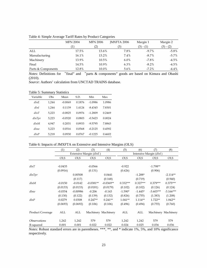
Our tariff data (𝑇𝑇) are taken from the UNCTAD TRAINS database through the World

Integrated Trade Solution (WITS) website. ∆ln𝑇𝑇 is calculated by taking the difference between log

of Mexico’s Most-Favored Nation (MFN) applied tariffs in 2004 and log of its preferential tariffs

vis-à-vis Japan in 2006 under the JMXFTA. It should be noted that between 2004 and 2006, Mexico

has implemented unilateral liberalization by reducing its MFN tariffs vis-à-vis WTO member

countries. In fact, Mexico’s simple average MFN applied tariff rate dropped from 17.5% in 2004 to

13.6% in 2006, whereas its preferential tariff rates against Japan was 7.8% in 2006 (Table 4). This

suggests that while ∆ln𝑇𝑇 actually represents tariff-saving effect that Japanese exporters have

enjoyed after the enactment of the JMXFTA, it does not necessarily represent the preferential margin

for Japanese exporters. We therefore construct an alternative variable ∆ln𝑇𝑇𝑝𝑝𝑇𝑇 , which is the

difference between log of Mexico’s MFN tariffs in 2006 and log of its preferential tariffs applied on

imports from Japan in 2006.

Data on Mexico’s imports from the world (𝑀𝑀) are taken from the Trade Map, developed

by the UNCTAD/WTO International Trade Center (ITC). Data on Japan’s wage rates by sector (w)

are drawn from the UNIDO’s International Yearbook of Industrial Statistics for manufacturing

sector and from the OECD’s STAN Structural Analysis Database for agricultural, forestry, fishing,

and mining sector, and converted from ISIC revision 3 product classifications to version 2002 of HS

code, using a converter provided by the WITS. We also obtain the data on price index by sector in

Mexico (𝑃𝑃) from the OECD’s STAN. The summary statistics for the variables, which will be

included in our estimation in the next subsection, are shown in Table 5.

5.3 Results

Using Monte Carlo simulations, Silva and Tenreyro (2006) showed that under

15

heteroskedasticity, parameters of log-linearized models estimated by OLS are severely biased, and

proposed to use Pseudo Poisson Maximum Likelihood (PPML) estimator in estimating the gravity

equations, in order to deal with the zero trade issues. However, we use OLS estimator because all the

variables in the estimation equations (8)’ and (9)’ including dependent variables ∆𝑙𝑙𝑙𝑙𝐸𝐸 and ∆𝑙𝑙𝑙𝑙𝐼𝐼

are time difference variables rather than level variables, meaning ∆𝑙𝑙𝑙𝑙𝐸𝐸 = 0 and ∆𝑙𝑙𝑙𝑙𝐼𝐼 = 0 in an

sector do not necessarily mean the level of export in the sector equals zero.

Table 6 reports the results from our baseline OLS models estimating the impacts of tariff

reduction under the JMXFTA on Japan’s exports. Separate regressions are presented for two

alternative tariff variables 𝑑𝑑𝑙𝑙𝑙𝑙𝑇𝑇 and 𝑑𝑑𝑙𝑙𝑙𝑙𝑇𝑇𝑝𝑝𝑇𝑇 for two different dependent variables – extensive

margin (dlnE) and intensive margin (dlnI). Results in columns (1) and (5) of Table 6 show that the

estimated coefficients for tariff reduction 𝑑𝑑𝑙𝑙𝑙𝑙𝑇𝑇 are not statistically significant in either extensive or

intensive margin regressions. On the other hand, column (6) indicates that if we use 𝑑𝑑𝑙𝑙𝑙𝑙𝑇𝑇𝑝𝑝𝑇𝑇 as an

independent variable, the tariff coefficient in the intensive margin regression becomes negative and

statistically significant at the 10% level, whereas that in the extensive margin regression is

statistically insignificant (column (2)). The coefficients for sector-level income, wage rate, and price

index in column (6) have the expected signs and are all statistically significant.

In Table 6, regression equations (3), (4), (7) and (8) focus on the sample of machinery

products. Machinery is the major export items of Japan and many of which are considered to be

differentiated products, therefore machinery exports are expected to react readily with the tariff

changes. Machinery products include all the goods classified as part of general machinery (HS 84),

electric machinery (HS 85), transport equipment (HS 86-89), and precision machinery (HS 90-92).

In the intensive margin equation (columns 7 and 8), the signs of coefficients of two tariff variables

show negative and statistically significant at 5% level. On the other hand, tariff coefficients of the

same tariff variables in the extensive margin regression are not statistically significant (columns 3

and 4). It is interesting to note that the sizes of the coefficients of tariffs in machinery (columns 7

and 8) are larger than the sizes of coefficients of tariffs in total export cases (columns 5 and 6). This

result support, as we expected, the idea that machinery exports are more sensitive to the tariff

changes rather than other export sectors. Other variables such as the proxy for industry demand

(dlnM), composite price index (dlnP) are correlated positively with intensive margins while the wage

rate (dlnw) correlates negatively with intensive margin. These all results in intensive margin case

support our hypotheses based on our theoretical model.

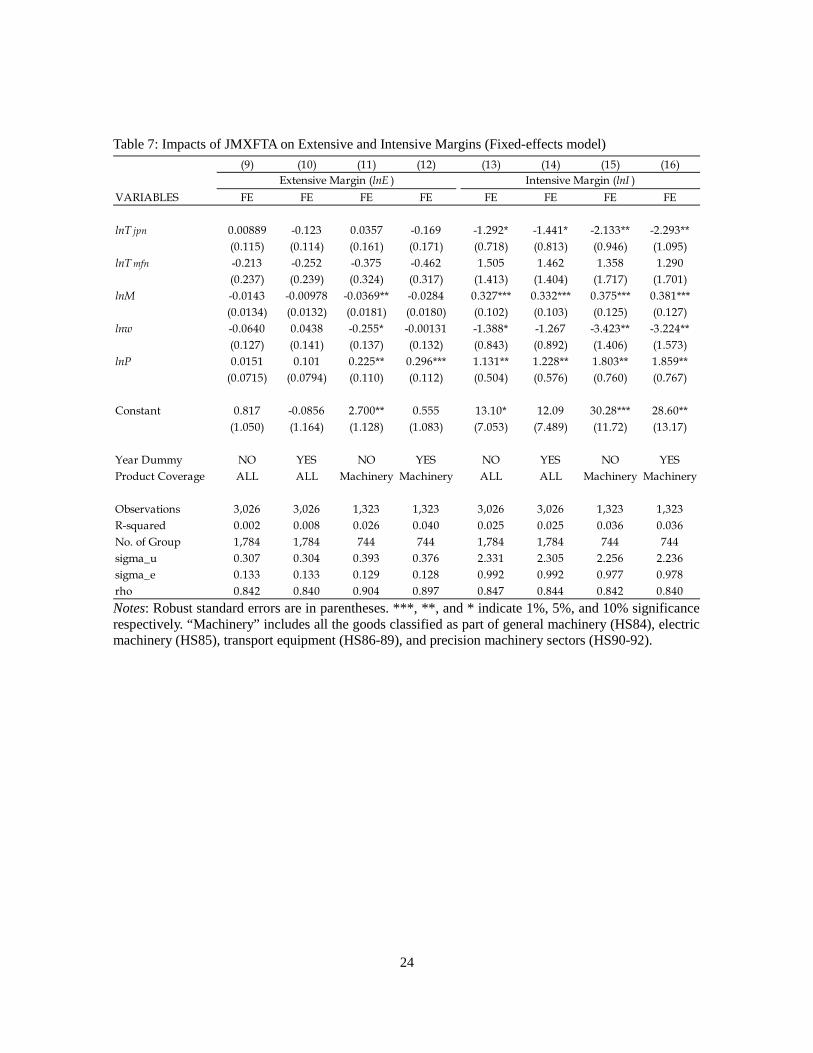
As a robustness check, we estimate product-specific fixed effects models. To do this, we

create and use a two-year panel dataset with level variables, rather than using a cross-section dataset with time difference variables. In particular, we introduce two tariff variables 𝑑𝑑𝑙𝑙𝑙𝑙𝑇𝑇𝑠𝑠𝑗𝑗𝑖𝑖 and

𝑑𝑑𝑙𝑙𝑙𝑙𝑇𝑇𝑚𝑚𝑚𝑚𝑖𝑖 in our estimation models, in order to capture the effects of Mexico’s preferential tariff

reduction vis-à-vis Japan while controlling the effects of Mexico’s unilateral liberalization vis-à-vis

16

WTO members as discussed in section 5.2. The results are shown in Table 7. Year fixed effects are included in the regressions (10), (12), (14), and (16). The coefficients for preferential tariff (𝑑𝑑𝑙𝑙𝑙𝑙𝑇𝑇𝑠𝑠𝑗𝑗𝑖𝑖)

in the intensive margin regressions remain negative and statistically significant at the 10% level for

all-products sample (column (13) and (15)), and at the 5% level for machinery products sample

(column (14) and (16)). On the contrary, tariff coefficients in the extensive margin regressions are

unstable and not statistically significant.

6. Summary and Conclusion This paper examines the impacts of JMXFTA on Japanese exports to Mexico. We construct

a theoretical trade model of heterogeneous firms, which is based on the Melitz-Chaney model, and

derive the theoretical relationship of the impacts of tariff changes on extensive and intensive trade

margins. Applying this model, the authors estimate the impacts of JMXFTA on product-level

extensive and intensive margins of Japan’s exports to Mexico by using the most detailed commodity

trade data.

We find that, in contrast to most previous studies, intensive margin rather than extensive

margin plays an important role in explaining the increase in trade volume caused by the FTA. The

reasons for this result appear to be twofold: First, our estimation uses the most detailed HS 9-digit

product level data rather than firm level data or country level data, which were used by many

previous studies adopting the Melitz and Chaney’s heterogeneous firm models. Those models

assume that each heterogeneous firm produces each differentiated product. However, one cannot

distinguish the intensive margin from extensive margin from only the information of the

firm-level-export data. For example, if a firm increases its export volume after tariff reduction, we

never know whether the firm expands export of goods it has previously exported or starts to export a

new good. According to the theory, the existing firms can never be new-goods-exporters. In other

words, the model predicts that if the existing firm increases its export after the policy change, the

export expansion is through the intensive margin, while if a new firm emerges (starts to export) after

the policy change, it is counted as the extensive margin, even if the new firm exports the same

product exported by the existing firm. Many of the literatures mentioned above often use

firm-level-export data and assume that the number of firms is a proxy for the extensive margin.

However, the number of firms does not equal to the number of products. The definition of extensive

margin is the number of new goods (not firms) introduced into the market. The number of firms,

therefore, cannot be a proxy for the extensive margin. In this paper, we correct this misalignment

between the theory and the empirical study.

Second, we use data of the year 2006, only one year after the enactment of JMXFTA. It

might be more time-consuming for exporters, even for existing exporters, to start exporting totally

new goods than trying to expand trade volume of existing traded goods, as they may have to bear

17

fixed costs including costs for searching and understanding information on preferential tariffs and

rules of origin, as well as costs for meeting rules of origin requirements. These transaction costs

would be much higher in the case of potential new exporters who do not have any experiences of

utilizing preferential tariffs or who are unaware that FTAs can be utilized as a corporate strategic tool.

If this were the case, a possible policy implication would be to reduce fixed costs, which potential

FTA users might face after the conclusion of new FTAs, through introducing less restrictive rules of

origin or providing user-friendly information for potential new FTA users. These policy initiatives

would contribute to trade expansion especially through extensive margins.

To conclude, we would like to touch upon two future research agendas. First, although our

study mainly focused on the impacts of JMXFTA on exports from Japan to Mexico, the impacts of

other FTAs such as NAFTA, should be also taken into account when estimating impacts of JMXFTA

on Japan’s exports. Second, the impacts of domestic policies in Mexico such as PROSEC (the

Program of Sectoral Promotion) in automotive industry should be considered, as it might also affect

bilateral trade and investment flow between the two countries.

18

References

1. Amurgo-Pacheco, A., and Pierola, M. D. (2008), “Patterns of export diversification in

developing countries: intensive and extensive margins.” Policy research working paper series,

No. 4473. The World Bank.

2. Ando M. and Urata S. (2011), “Impacts of the Japan=Mexico EPA on Bilateral Trade,” REITI

Discussion Paper 11-E-020.

3. Arkolakis, C. (2010). “Market penetration costs and the new consumer margin in international

trade.” Journal of Political Economy, 118(6), 1151-1199.

4. Arkolakis, C., Costinot, A., and Rodríguez-Clare, A. (2012). “New trade models, same old

gains?” American Economic Review 102(1), 94-130.

5. Besedes, T., and Prusa, T. J. (2013). “The role of extensive and intensive margins and export

growth.” Journal of Development Economics, 96(2), 371-379.

6. Buono, I. and Lalanne, G. (2012). “The effect of the Uruguay round on the intensive and

extensive margins of trade.” Journal of International Economics 86(2), 269-283.

7. Chaney, T. (2008). “Distorted Gravity: The intensive and extensive margins of international

trade.” American Economic Review 98(4), 1707–21.

8. Crozet, M. and Koenig, P. (2010). “Structural gravity equations with intensive and extensive

margins.” Canadian Journal of Economics, 43(1), 41-62.

9. Debaere, P., and Mostashari, S. (2010). “Do tariffs matter for the extensive margin of

international trade? An empirical analysis.” Journal of International Economics, 81(2), 163-169.

10. Dutt, P., Mihov, I., and van Zandt, T. (2013). “The effect of WTO on the extensive and intensive

margins of trade.” Journal of International Economics, 91(2), 204-219.

11. Evenett, S. J. and Venables, A. J. (2002). “Export growth in developing countries: market entry

and bilateral trade flows.” Working paper, University of Bern.

12. Feenstra R. C. (1994). “New product varieties and the measurement of international prices.”

American Economic Review, 84(1), 157-177.

13. Feenstra R. C. (2010). Product Variety and the Gains from International Trade. MIT Press,

Cambridge, MA.

14. Fellbermyr, G. J., and Kohler, W. (2006). “Exploring the intensive and extensive margins of

world trade.” Review of World Economics, 142(4), 642-674.

15. Foster, N. (2012). “Preferential trade agreements and the margins of Imports.” Open Economies

Review, 23(5), 869–889.

16. Frankel, J. and Romer, D. (1999). “Does trade cause growth?” American Economic Review

89(3), 379-399.

17. Helpman, El., Melitz, M. and Rubinstein, Y. (2008). “Estimating trade flows: trading partners

19

and trading volumes.” Quarterly Journal of Economics 123(2): 441–87.

18. Hillberry, R. H., and McDaniel, C. A. (2002). “”A decomposition of North American trade

growth since NAFTA.” Working paper, U.S. International Trade Commission.

19. Hummels, D. and Klenow, P. J. (2005). “The variety and quality of a nation’s exports.”

American Economic Review, 95(3), 704-723.

20. Kehoe Timothy J. and Ruhl, Kim J. (2013). “How important is the new goods margin in

international trade?” Journal of Political Economy, 121(2), 358-392.

21. Kimura, F and Obashi, A. (2010) “International Production Networks in Machinery Industries:

Structure and Its Evolution.” ERIA Discussion Paper Series (ERIA-DP-2010-09), Economic

research Institute for ASEAN and East Asia (ERIA).

22. Krueger, A. (1997). “Trade policy and development: how we learn.” American Economic

Review 87(1), 1-22.

23. Melitz, M. (2003) “The impact of trade on intra-industry reallocations and aggregate industry

productivity.” Econometrica 71(6), 1695–725.

24. Romalis, J. (2007). “NAFTA’s and CUSFTA’s impact on international trade.” Review of

Economics and Statistics, 89(3), 416-435.

25. Sachs, J. D. and Warner, A. (1995). “Economic reform and the process of global integration.”

Brookings Papers on Economic Activity 1995(1), 1-118.

26. Silva, J. M. C. S and Tenreyro, S. (2006) “The Log of Gravity.” Review of Economics and Statistics, 88(4), 641-58.

27. Urata, S. and M. Okabe (2013) “Trade Creation and Diversion Effects of Regional Trade Agreements: A Product-Level Analysis.” World Economy, 37(2), 267-289.

20

Figure 1: Japan's Exports to Mexico by Major Products

Source: Trade Statistics of Japan, Ministry of Finance.

Table 1: Patterns of Japanese Exports to Mexico in 2004 and 2006

Source: Computed from Trade Statistics of Japan, Ministry of Finance.

0

200

400

600

800

1,000

1,200

2000 2002 2004 2006 2008 2010 2012

OthersChemical products & plasticsPrecision machineryBase metalsTransport machineryGeneral & electricc machinery

(Billion JPY)

21

Table 2: Patterns of Japanese Exports to Mexico by Products in 2004 and 2006 (No. of Products)

Notes: yy: exported in 2004 and 2006, yn: exported in 2004 only, ny: exported in 2006 only, nn: never exported. Source: Authors’ calculation from Trade Statistics of Japan, Ministry of Finance.

yy yn ny yy+yn+ny nn 1. live animals/animal products 0 2 2 4 183 187 2. vegetable products 2 0 2 4 222 226 3. animal/vegetable fats, oils, & waxes 3 0 0 3 46 49 4. prepared foodstuffs, beverages, & tobacco 15 5 8 28 185 213 5. mineral products 5 6 5 16 142 158 6. products of the chemical or allied industries 171 43 51 265 564 829 7. plastics & rubber 121 19 26 166 105 271 8. raw hides and skins, leather 4 2 1 7 88 95 9. wood, cork, & straw 2 2 3 7 81 88 10. wood pulp wood, paper 35 8 7 50 117 167 11. textiles 72 44 50 166 921 1,087 12. footwear, umbrellas, etc. 0 1 1 2 60 62 13. stone, cement, ceramic, & glass 38 10 18 66 95 161 14. pearls, precious stones/metals 2 6 1 9 55 64 15. base metals 228 63 69 360 409 769 16. machinery and electrical equipment 547 100 77 724 327 1,051 17. transport equipment 43 6 13 62 136 198 18. optical, precision, & medicalinstruments 157 23 13 193 106 299 19. arms and ammunition 0 0 2 2 17 19 20. miscellaneous 48 7 14 69 81 150 21. art/antiques 0 1 3 4 3 7 Total 1,493 348 366 2,207 3,943 6,150

HS SectionTotal

(HS 9-digit)Category

22

Table 3: Patterns of Japanese Exports to Mexico by Products in 2004 and 2006 (Export value, million yen)

Notes: yy: exported in 2004 and 2006, yn: exported in 2004 only, ny: exported in 2006 only, nn: never exported. Source: Computed from Trade Statistics of Japan, Ministry of Finance.

yy04 yy06 yy06-yy04 yy06/yy04 yn04 yn06 ny04 ny06 nn04 nn06 1. live animals/animal products 0 0 0 12 0 0 21 0 0 2. vegetable products 2 3 2 1.8 0 0 0 1 0 0 3. animal/vegetable fats, oils, & waxes 6 13 7 2.1 0 0 0 0 0 0 4. prepared foodstuffs, beverages, & tobacco 114 349 235 3.1 5 0 0 6 0 0 5. mineral products 81 107 26 1.3 905 0 0 24 0 0 6. products of the chemical or allied industries 11,980 13,702 1,722 1.1 272 0 0 801 0 0 7. plastics & rubber 17,191 22,497 5,306 1.3 138 0 0 641 0 0 8. raw hides and skins, leather 4 5 1 1.3 2 0 0 0 0 0 9. wood, cork, & straw 15 8 -7 0.5 4 0 0 11 0 0 10. wood pulp wood, paper 1,159 1,714 555 1.5 90 0 0 82 0 0 11. textiles 1,494 2,145 651 1.4 250 0 0 234 0 0 12. footwear, umbrellas, etc. 0 0 0 2 0 0 1 0 0 13. stone, cement, ceramic, & glass 3,634 10,833 7,198 3.0 18 0 0 607 0 0 14. pearls, precious stones/metals 17 238 221 13.6 21 0 0 1 0 0 15. base metals 64,006 103,873 39,867 1.6 5,009 0 0 3,456 0 0 16. machinery and electrical equipment 265,806 492,696 226,890 1.9 4,917 0 0 2,094 0 0 17. transport equipment 142,533 304,195 161,662 2.1 309 0 0 20,059 0 0 18. optical, precision, & medicalinstruments 28,766 43,338 14,572 1.5 182 0 0 326 0 0 19. arms and ammunition 0 0 0 0 0 0 4 0 0 20. miscellaneous 3,636 5,807 2,171 1.6 24 0 0 17 0 0 21. art/antiques 0 0 0 0 0 0 53 0 0 Total 540,444 1,001,524 461,080 40.9 12,160 0 0 28,440 0 0

yyHS Section

yn ny nn

23

Table 4: Simple Average Tariff Rates by Product Categories

Notes: Definitions for “final” and “parts & components” goods are based on Kimura and Obashi (2010). Source: Authors’ calculation from UNCTAD TRAINS database. Table 5: Summary Statistics

Table 6: Impacts of JMXFTA on Extensive and Intensive Margins (OLS)

Notes: Robust standard errors are in parentheses. ***, **, and * indicate 1%, 5%, and 10% significance respectively.

MFN 2004 MFN 2006 JMXFTA 2006 Margin 1 Margin 2(1) (2) (3) (3) - (1) (3) - (2)

ALL 17.5% 13.6% 7.8% -9.7% -5.8%Manufacturing 16.1% 13.2% 7.4% -8.7% -5.7%Machinery 13.9% 10.5% 6.0% -7.8% -4.5%Final 14.5% 10.9% 6.3% -8.2% -4.5%Parts & Components 12.8% 10.0% 5.6% -7.2% -4.4%

Variable Obs Mean S.D. Min Max

dlnE 1,244 -0.0069 0.1876 -1.0986 1.0986

dlnI 1,244 0.1139 1.4124 -8.4345 7.8301

dlnT 5,223 -0.0825 0.0976 -1.2809 0.2469

dlnTpr 5,223 -0.0520 0.0803 -0.5423 0.0024

dlnM 4,947 0.2031 0.8933 -9.5795 7.8843

dlnw 5,223 0.0516 0.0568 -0.2125 0.4592

dlnP 5,218 0.0930 0.0767 -0.1225 0.4602

(1) (2) (3) (4) (5) (6) (7) (8)

OLS OLS OLS OLS OLS OLS OLS OLS

dlnT -0.0435 -0.0566 -0.922 -1.798**(0.0916) (0.131) (0.626) (0.906)

dlnTpr 0.00508 0.0441 -1.288* -2.114**(0.117) (0.168) (0.719) (0.940)

dlnM -0.0150 -0.0142 -0.0381** -0.0369** 0.332*** 0.327*** 0.379*** 0.375***(0.0133) (0.0133) (0.0181) (0.0179) (0.102) (0.102) (0.126) (0.124)

dlnw -0.0354 -0.00986 -0.206 -0.143 -1.590* -1.445* -3.603*** -3.166***(0.130) (0.122) (0.139) (0.132) (0.826) (0.755) (1.383) (1.208)

dlnP 0.0279 0.0308 0.247** 0.241** 1.041** 1.114** 1.722** 1.842**(0.0693) (0.0692) (0.106) (0.106) (0.496) (0.494) (0.755) (0.760)

Product Coverage ALL ALL Machinery Machinery ALL ALL Machinery Machinery

Observations 1,242 1,242 579 579 1,242 1,242 579 579R-squared 0.001 0.001 0.022 0.022 0.024 0.025 0.036 0.036

Extensive Margin (dlnE ) Intensive Margin (dlnI )

24

Table 7: Impacts of JMXFTA on Extensive and Intensive Margins (Fixed-effects model)

Notes: Robust standard errors are in parentheses. ***, **, and * indicate 1%, 5%, and 10% significance respectively. “Machinery” includes all the goods classified as part of general machinery (HS84), electric machinery (HS85), transport equipment (HS86-89), and precision machinery sectors (HS90-92).

(9) (10) (11) (12) (13) (14) (15) (16)

VARIABLES FE FE FE FE FE FE FE FE

lnT jpn 0.00889 -0.123 0.0357 -0.169 -1.292* -1.441* -2.133** -2.293**(0.115) (0.114) (0.161) (0.171) (0.718) (0.813) (0.946) (1.095)

lnT mfn -0.213 -0.252 -0.375 -0.462 1.505 1.462 1.358 1.290(0.237) (0.239) (0.324) (0.317) (1.413) (1.404) (1.717) (1.701)

lnM -0.0143 -0.00978 -0.0369** -0.0284 0.327*** 0.332*** 0.375*** 0.381***(0.0134) (0.0132) (0.0181) (0.0180) (0.102) (0.103) (0.125) (0.127)

lnw -0.0640 0.0438 -0.255* -0.00131 -1.388* -1.267 -3.423** -3.224**(0.127) (0.141) (0.137) (0.132) (0.843) (0.892) (1.406) (1.573)

lnP 0.0151 0.101 0.225** 0.296*** 1.131** 1.228** 1.803** 1.859**(0.0715) (0.0794) (0.110) (0.112) (0.504) (0.576) (0.760) (0.767)

Constant 0.817 -0.0856 2.700** 0.555 13.10* 12.09 30.28*** 28.60**(1.050) (1.164) (1.128) (1.083) (7.053) (7.489) (11.72) (13.17)

Year Dummy NO YES NO YES NO YES NO YESProduct Coverage ALL ALL Machinery Machinery ALL ALL Machinery Machinery

Observations 3,026 3,026 1,323 1,323 3,026 3,026 1,323 1,323R-squared 0.002 0.008 0.026 0.040 0.025 0.025 0.036 0.036No. of Group 1,784 1,784 744 744 1,784 1,784 744 744sigma_u 0.307 0.304 0.393 0.376 2.331 2.305 2.256 2.236sigma_e 0.133 0.133 0.129 0.128 0.992 0.992 0.977 0.978rho 0.842 0.840 0.904 0.897 0.847 0.844 0.842 0.840

Extensive Margin (lnE ) Intensive Margin (lnI )