University of North DakotaUND Scholarly Commons

Theses and Dissertations Theses, Dissertations, and Senior Projects

January 2014

Estimating The Effect Of Poverty On ViolentCrimeJose Gabriel Ramos

Follow this and additional works at: https://commons.und.edu/theses

This Thesis is brought to you for free and open access by the Theses, Dissertations, and Senior Projects at UND Scholarly Commons. It has beenaccepted for inclusion in Theses and Dissertations by an authorized administrator of UND Scholarly Commons. For more information, please contactzeineb.yousif@library.und.edu.

Recommended CitationRamos, Jose Gabriel, "Estimating The Effect Of Poverty On Violent Crime" (2014). Theses and Dissertations. 1696.https://commons.und.edu/theses/1696

ESTIMATING THE EFFECT OF POVERTY ON VIOLENT CRIME

by

Jose Gabriel Ramos Bachelor of Arts, Florida International University, 1997

Master of Business Administration, Florida International University, 2002

A thesis

Submitted to the Graduate Faculty

of the

University of North Dakota

in partial fulfillment of the requirements

for the degree of

Master of Science in Applied Economics

Grand Forks, North Dakota August 2014

Copyright 2014 Jose Ramos

ii

PERMISSION

Title Estimating the Effect of Poverty on Violent Crime Department Economics Degree Master of Science in Applied Economics

In presenting this thesis in partial fulfillment of the requirements for a graduate degree from the University of North Dakota, I agree that the library of this University shall make it freely available for inspection. I further agree that permission for extensive copying for scholarly purposes may be granted by the professor who supervised my thesis work or, in his absence, by the Chairperson of the department or the dean of the School of Graduate Studies. It is understood that any copying or publication or other use of this thesis or part thereof for financial gain shall not be allowed without my written permission. It is also understood that due recognition shall be given to me and to the University of North Dakota in any scholarly use which may be made of any material in my thesis.

Jose Ramos June 28, 2014

iv

TABLE OF CONTENTS

LIST OF FIGURES ........................................................................................................... vi

LIST OF TABLES ............................................................................................................ vii

ABSTRACT ..................................................................................................................... viii

CHAPTER

I. INTRODUCTION .......................................................................................1

II. LITERATURE REVIEW AND BACKGROUND .....................................6

III. DATA AND METHODOLOGY ...............................................................11

IV. RESULTS ..................................................................................................21

V. CONCLUSION .........................................................................................30

REFERENCES ..................................................................................................................31

v

LIST OF FIGURES

Figure Page

1. Poverty rates in the U.S ...................................................................................................2

2. Violent Crime rates in the U.S .........................................................................................3

3. Change in Violent Crime and Law Enforcement personnel in the U.S ..........................4

vi

LIST OF TABLES

Table Page

1. Variables and summary statistics ..................................................................................14

2. Correlation diagnostics between violent crime rates and explanatory variables ..........17

3. Multicollinearity diagnostics results of explanatory variables .....................................19

4. State fixed effects results on violent crime rates ..........................................................22

5. State and time fixed effects results on violent crime rates ............................................24

6. State and time fixed effects results of poverty rates on violent crime rates .................26

7. Regression results for individual violent crime categories ...........................................27

vii

ABSTRACT

I examine the effect of poverty on violent crime in the United States during the years

between 2000 and 2012. My analysis contributes to the literature by utilizing state-level

poverty rates as the main variable of interest, and directly studying its effect on violent

crime rates. I use panel data and a group (state) and time fixed effects estimation method

in the study. The results confirm prior research that concludes that poverty does not have

a significant effect on violent crime.

viii

CHAPTER I

INTRODUCTION

In the literature, some researchers have developed a theory of crime by creating

economic models that explain illegal behavior. Others have focused on analyzing

historical data to measure and identify the determinants of crime. The effect of the

business cycles on various measures of crime has also been an important part of the

research on this topic.

However, not much research has focused specifically on the relationship between

poverty and violent crime. For example, Huang, Laing and Wang (2004) propose a

dynamic general equilibrium model to understand the link between crime and poverty,

but poverty rates do not figure anywhere in their model. Bjerk (2010) found a connection

between individual poverty and property and violent crimes, where his focus was

neighborhood poverty and economic segregation. The poverty rate was not the main

independent variable in Bjerk’s study. A brief review of the related literature, which we

detail in chapter II, suggests that poverty has been indirectly linked to crime rates via

proxy economic indicators, such as the per capita income and the unemployment rate.

In the popular mass-media on the other hand, there are reports supporting the link

between crime and poverty. For example, Blaine and Sauter (2013) suggest the existence

of a relationship between violent crime and poverty in their well-publicized article “The

Most Dangerous States in America”, which was reproduced by several news outlets.

1

They pointed out that “of the 10 states with the highest rates of violent crime, eight have

lower rates of adults with bachelor’s degrees, and most of them had median income

levels below the national figure in 2012”1.

A quick glance at the poverty and violent crime rate data for the years 2000 –

2012 leaves us with a taste of uncertainty between these two factors.

Figure 1. Poverty rates in the U.S. Source: U.S. Bureau of the Census.

1 Blaine, C. & Sauter, M. (October 4, 2013). The Most Dangerous States in America. 24/7 Wall St. Available at:

http://247wallst.com/special-report/2013/10/04/the-most-dangerous-states-in-america

02

46

810

1214

16P

erce

nt in

Pov

erty

2000 2005 2010 2015Year

poverty rate

Period 2000 - 2012Poverty rates in the U.S.

2

During the 13-year period covered by Figure 1, poverty rates have been consistently

increasing in the United States, from a low of 11.3% in the year 2000 to a high of 15% in

2012. The highest jump seems to have occurred in 2007/2008 and the rate stabilized

around the year 2010. This behavior, which officially started in December of 2007 and

ended in June of 2009, coincided with the worst of the great recession.

When we look at different types of violent crimes, which are displayed in Figure

2, we observe a trend that is in the opposite direction during that same period.

Figure 2. Violent Crime rates in the U.S. Source: Federal Bureau of Investigation

Uniform Crime Reports (UCR)

For example, the overall violent crime rate decreased by roughly 20% between 2000 and

2012. Among others, rape and murder rates remained fairly constant, while robbery and

010

020

030

040

050

0C

rimes

per

100

000

2000 2005 2010 2015Year

aggravated assault murder rape

robbery violent crime

Period 2000 - 2012Violent Crime rates in the U.S.

3

aggravated assault rates dropped, especially the latter one. The reported data does not

seem to support the positive link between poverty and violent crimes, as media outlets

tend to propagate. There are certainly other factors at work that could explain the

dramatic drop in violent crime in the last decade, and they could be possibly “cancelling”

out the negative effect of poverty. A counterintuitive representation of our data is the

comparison between the changes in violent crime rates and law enforcement personnel.

As we can see from Figure 3 they both decreased in the period between 2000 and 2012.

Figure 3. Change in Violent Crime and Law Enforcement personnel in the U.S.

Source: Federal Bureau of Investigation

5.8

5.9

66.

16.

2R

ate

Cha

nge

2000 2005 2010 2015Year

violent crime

law enforcement personnel

Period 2000 - 2012Violent Crime and Law enforcement personnel in the U.S.

4

In this research, I intend to fill the gap in the literature and study the effect

poverty has on violent crime at an aggregate level, with poverty rates as the central

variable of interest. Given the initial direction of the data, it is possible that poverty rates

may not be an appropriate variable to use at the aggregate level, and instead a different

economic indicator may have to be selected as a proxy for poverty levels.

My data-driven approach relies on contemporary econometric methods and

existing theory. The expected results are that the poverty rates are strongly related to

robberies but less so to aggravated assaults, murders and rapes. Also, the overall

relationship between poverty and violent crime rates should not be statistically

significant.

As a resident of Tennessee, the state with the highest violent crime rate in the

country in 2012, this topic is of particular interest to me. If it is found that poverty does

have a significant positive effect on violent crime, then the implication for policy-making

is that reduction in poverty levels should go together with law enforcement initiatives in

the pursuit of combating and reducing violent crime in the state. On the other hand, if

poverty has a negative effect on violent crimes or no effect at all, efforts should be made

to identify and study other variables that could have an impact in lowering the violent

crime rates in the state.

5

CHAPTER II

LITERATURE REVIEW AND BACKGROUND

Among the numerous research that studies crime using alternative economic

methods, probably the most widely quoted paper is "Crime and Punishment: an

Economic Approach" by Gary Becker (1968). Becker (1968) developed a model of

crime to find optimal public and private policies to combat illegal behavior using

economic analysis. According to Becker’s model, criminal acts result from a rational

decision based on a cost-benefit analysis. As noted by Fajnzylber, Lederman and Loayza

(2002), the expected benefits are given by the difference between the loot and the

opportunity cost of crime; and the costs are given by the penalties imposed to

apprehended criminals. The model’s deterrence theory is that an increase in a typical

offender’s chance of being caught decreases crime. This intuitive prediction is at the core

of many papers that mention Becker’s research as seminal and as the starting point of

analyzing crime using economic methods.

Departing from Becker’s original model, Cantor and Land (1985) focused their

research in studying whether economic conditions had an effect on crime. Using annual

time-series data for the United States and the unemployment rate as a proxy for economic

activity, they found a significant effect of the business cycles on crime. Their theoretical

model, which used the criminal motivation and criminal opportunity effects, became the

foundation for two decades of empirical research into the relationship between economic

6

conditions and crime. Social strain and social controls are two of the sociological

theories that support the relationship between criminal motivation and economic

conditions.

Social strain is “the pressure individuals feel to reach socially determined goals”

(Arvanites & Defina, 2006, p. 141). When these goals become out of reach via legal

means, individuals are pressured to make use of illegitimate means to achieve them. For

example, if we measure success in our society by the level of material wealth, an

individual must have a good paying job or another source of legitimate income to be

successful. When economic conditions are deteriorating, “success” becomes more

elusive. Therefore, criminal motivation can arise from social strain.

Social control is usually described as “the ability of society to regulate its

members” (Arvanites & Defina, 2006, p. 142). The lives of people are structured by

work, parents, friends, stores, churches, libraries, etc. that provide routines, expectations

and social support networks. If a person loses his/her job, the social aspect of work is

greatly reduced. These institutions depend on the support of the people, and when

economic conditions worsen, people cannot provide them with the same level of

resources they are used to, weakening them. A result of that fact is that social control

diminishes and criminal activities rise.

Besides motivation, the economic conditions also influence the opportunity to

commit crimes. For example, in an improving economy, more wealth is generated and

people are busy working or taking part in activities away from their homes. This creates

the opportunity for criminals to target empty homes.

7

Based on the prior definitions Cantor and Land (1985) conclude that the criminal

opportunity effect will run counter to the criminal motivation effect.

Prior to Cornwell and Trumbull’s (1994) economic model of crime, estimating

and testing what type of economic models was done using aggregate data, usually at the

state or national level, with cross-sectional econometric techniques. Cornwell and

Trumbull (1994, p. 360) argued that “ideally, the economic model of crime should be

estimated with individual level data since the model purports to describe the behavior of

individuals”. Instead, they became one of the first to use county-level data for a lower

level of aggregation, as well as panel data to control for unobserved heterogeneity.

In a related paper, Gould, Weinberg and Mustard (2002) examine the impact of

both wages and unemployment on crime and found that even though those two factors are

significantly related to crime, wages played a larger role in the crime trends in the last

few decades. Their research not only focused on property crimes but also included

violent crimes. They used county-level panel data and instrumental variables in their

analysis.

Levitt (2004) studies the reasons why crime fell in the 1990s. He identifies four

factors that appear to explain the drop in crime: increased incarceration, more police, the

decline of crack and legalized abortion. Other factors often cited as important reasons for

the decline do not appear to have played an important role: the strong economy, changing

demographics, innovative policing strategies, gun laws and increased use of capital

punishment.

8

Arvanites and Defina (2006) reexamine Cantor and Land’s (1985) work to

analyze the influence of business cycle fluctuations on street crime. Instead of using the

unemployment rate as a proxy for economic strength, as previous studies had done,

Arvanites and Defina (2006) determine that the inflation-adjusted per capita gross state

product is a better measure of business cycle conditions. Using fixed-effects panel

models, they find that a strong economy has a negative and statistically significant effect

on property crimes and robbery - the only violent crime with a purpose of financial gain.

The conclusion that the “stronger economy of the 1990s contributed to reductions in

crime” (Arvanites & Defina, 2006, p. 161) is in stark contrast to Levitt’s (2004) assertion

that the strong economy did not play an important role in the decline of crime during the

same period.

Violent crime was specifically targeted by Rosenfeld (2009), who proposes that

the economy stimulates violent crime indirectly through its effect on acquisitive crime.

He questions social strain and social control theories because they imply that violent and

property crimes are spuriously associated and they don’t acknowledge the possibility of a

causal connection between the two types of crime. Citing prior research by LaFree

(1998), Rosenfeld (2009) notes that property and violent crime rates track one another

closely over time, and that involvement in property crime is an important risk factor for

violent victimization, including homicide. The existence of “underground” markets,

where stolen goods are traded, contribute to the rise of violent crimes because violence is

the main mode of enforcement of agreements in this space. Rosenfeld (2009) uses fixed-

effects panel models of change in acquisitive crime and homicide rates to evaluate his

hypothesis. The findings include a significant effect of acquisitive crime on homicide,

9

which put pressure on studies that deny that economic conditions do not have an effect on

violent crimes other than robbery.

Interestingly, poverty is not directly used as one of the principal factors affecting

crime rates in the literature reviewed. Rather, it is implicit in the economic factors that

are part of the various studies on crime. Bjerk (2010) is the only work that comes close

with his model of crime, poverty and neighborhood composition. He concludes that

“violent criminal behavior of poor individuals may be more influenced by their

neighborhood economic characteristics than is the violent criminal behavior of non-poor

individuals” (Bjerk, 2010, p. 243).

Therefore, my research not only complements the existing literature but also

extends it to a new direction.

.

10

CHAPTER III

DATA AND METHODOLOGY

Ideally, individual level data should be used when estimating an economic model

of crime, since crime is the result of individual behavior. Data at the county or zip codes

or metropolitan area level are preferred to aggregate level, such as state or national data.

Due to difficulty in obtaining reliable annual poverty rate data prior to 2005, as well as

data for other variables of interest, this paper uses state-level data for empirical work.

Data for this study covers the 13 year period 2000 – 2012 for each of the 50 states.

Because the District of Columbia technically is not a state, it is excluded from the dataset.

A more appropriate place to include Washington D.C. should be a study of crime

comparing different metropolitan areas.

The FBI’s Uniform Crime Report (UCR) is the source of data on violent crime

rates, both for aggregate and individual categories (robbery, assault, murder, etc.). The

annual report “Crime in the United States”, from the same agency, provided information

on state law enforcement personnel. The Census Bureau is the source of data for poverty

rates, population growth rates, population aged 15-24, race and Hispanic origin, and

educational attainment levels. The Bureau of Economic Analysis is the source of

information on state GDP per capita and the National Bureau of Economic Research

11

(NBER) provided data on business cycles reference dates. In all, we have 650 observations

per variable for a total of more than 7000 observations to work with.

Besides poverty rates, additional explanatory variables were selected based on prior

studies and theories from the existing literature. State GDP per capita, state law

enforcement per 100,000 population and population aged 15-24, also known as the “crime

age”, were selected following Rosenfeld’s (2009) study on economic conditions and

homicides. Arvanites and Defina (2006) also include a similar “crime age” variable in

their model although their age range was 17-24. Gould, Weinberg and Mustard (2002)

make use of multiple variables related to educational attainment when studying the

relationship between crime and labor market conditions for less educated men. The

variable population growth rate is included in my model based on the assumption that a

larger population could result in more crimes reported, but not necessarily greater crime

rates. Finally, race and ethnicity variables have been used by Arvanites and Defina (2006)

and by Cornwell and Trumbull (1994). The categories selected in this paper, non-Hispanic

white, non-Hispanic black and Hispanic, are the ones used by the Bureau of Justice

Statistics in their prisoner census data.

The following equation (1) is our preliminary regression specification:

VCit= β0 + β1POVi,t+ β2POVi,t-1+ β3GDPi,t+ β4POPi,t+ β5AGEDi,t+ β6LAWENFi,t+

β7HSGRADi,t+ β8WHTi,t + β9BLKi,t + β10HISi,t + Ui,t (1)

12

where the main dependent variable VCi,t is the violent crime rate in state i at time t.

Among the set of main explanatory variables, POVi,t is the poverty rate in state i at time

t, POVi,t-1 is the lagged poverty rate in state i at time t-1, GDPi,t is the GDP per capita in

2005 chained dollars in state i at time t, POPi,t is the population growth rate in state i at

time t expressed as a percentage, AGEDi,t is the percentage of the population aged 15-24

years in state i at time t, LAWENFi,t is the law enforcement personnel per 100,000 in

state i at time t, HSGRADi,t is the percentage of the population 25 years and older that

graduated high school in state i at time t, WHTi,t is the percentage of the population that

is non-Hispanic white in state i at time t, BLKi,t is the percentage of the population that is

non-Hispanic black in state i at time t, HISi,t is the percentage of the population that is

Hispanic of any race in state i at time t, and Ui,t is the error term.

Separately, I test regressions (1) for secondary dependent variables for 4 different

categories of violent crime: robbery rates (RBit), aggravated assault rates (AAit), murder

rates (MUit) and rape rates (RPit). These secondary regressions have the same

explanatory variables as Equation 1. The only difference is the dependent variable on the

left hand side. Cherry and List (2002) argue that economic models of crime suffered

from aggregation bias and it isn’t appropriate to pool different crime types into a single

decision model. Therefore, running separate regressions for specific categories of violent

crime in addition to the aggregate violent crime rate is an effective attempt to address this

issue.

All variables included in this study are summarized in Table 1.

13

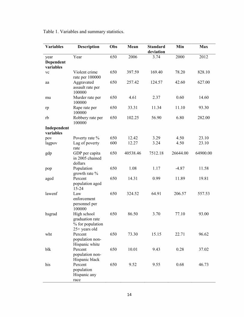
Table 1. Variables and summary statistics.

Variables Description Obs Mean Standard deviation

Min Max

year Year 650 2006 3.74 2000 2012 Dependent variables

vc Violent crime rate per 100000

650 397.59 169.40 78.20 828.10

aa Aggravated assault rate per 100000

650 257.42 124.57 42.60 627.00

mu Murder rate per 100000

650 4.61 2.37 0.60 14.60

rp Rape rate per 100000

650 33.31 11.34 11.10 93.30

rb Robbery rate per 100000

650 102.25 56.90 6.80 282.00

Independent variables

pov Poverty rate % 650 12.42 3.29 4.50 23.10 lagpov Lag of poverty

rate 600 12.27 3.24 4.50 23.10

gdp GDP per capita in 2005 chained dollars

650 40538.46 7512.18 26644.00 64900.00

pop Population growth rate %

650 1.08 1.17 -4.87 11.58

aged Percent population aged 15-24

650 14.31 0.99 11.89 19.81

lawenf Law enforcement personnel per 100000

650 324.52 64.91 206.57 557.53

hsgrad High school graduation rate % for population 25+ years old

650 86.50 3.70 77.10 93.00

wht Percent population non-Hispanic white

650 73.30 15.15 22.71 96.62

blk Percent population non-Hispanic black

650 10.01 9.43 0.28 37.02

his Percent population Hispanic any race

650 9.52 9.55 0.68 46.73

14

All variables show a certain amount of variation. Poverty rates had a fairly low standard

deviation of 3.70, where the lowest poverty rate was 4.50% and belonged to New

Hampshire in the year 2000; the highest poverty rate in our data set was 23.10%, which

belonged to Mississippi in the year 2009. In those same years, the violent crime rate for

New Hampshire was 175.4 and for Mississippi was 286.3. In both instances, well below

the mean violent crime rate of 397.59 for the 13-year period between 2000 and 2012.

Could this be an indication that there is no relationship between poverty and violent

crime? Another variable, the percentage of the population aged 15-24 years, had the

smallest standard deviation of 0.99, indicating most of its data is clustered around the

mean of 14.31%. Connecticut had the smallest share of its population between ages 15-

24 in the year 2000, at 11.89%, while Utah had the largest concentration of young people

in the years 2000 and 2001, with 19.82% of its population in that age bracket. The

violent crime rates for these states in the year 2000 were 324.7 and 255.7 respectively.

The variable per capita GDP had the largest dispersion around its mean, with a standard

deviation of 7,512.18. Expressed in 2005 chained dollars, Delaware had the highest per

capita GDP in 2007 at $64,900 while Mississippi had the lowest per capita GDP in 2001

at $26,644. In those same years, the violent crime rate for Delaware was 705.4 and for

Mississippi was 349.9. This suggests a possible positive relationship between per capita

GDP and violent crime rates.

The estimation method selected for this study is the fixed effects method. None

of the explanatory variables are time-invariant, a requirement for using this method.

Panel data allows us to control for unobserved heterogeneity, which decreases the chance

for endogeneity, where the explanatory variable is correlated with the error term of the

15

regression. The fixed effects estimator allows for arbitrary correlation between the

unobserved effects and the explanatory variables in any time period (Wooldridge, 2013,

Ch. 14). Using changes within each group (states) from our panel, the fixed effects can

be eliminated by subtracting the individual means of the variables in the model. The

alternative random effects method assumes there is no correlation between the

unobserved effects and the explanatory variables. However, as Wooldridge (2013, p.

496) points out, “we cannot treat our sample as a random sample from a large population,

especially when the unit of observation is a large geographical unit”, which in our case is

a state. Because we have data for 13 years, an additional regression that also includes

time fixed effects will be tested. This regression results in adding year dummies, except

for the first year, to our original state fixed effects regression.

Natural logarithms are applied to our dependent variables and to the explanatory

variables real GDP per capita and law enforcement personnel. This helps to achieve

stationarity in the time-series part of the data, transform any non-linear distributions and

normalize data where non-normal distributions are present (Yearwood & Koinis, 2011).

The remaining variables are already given as percentages so there is no need to apply

logarithmic transformations. After transformation, the regression equation (1) becomes

equation (2):

Ln(VCi,t)= β0 +β1POVi,t+β2POVi,t-1+β3Ln(GDPi,t)+β4POPi,t+β5AGEDit+β6Ln(LAWENFi,t)+

β7HSGRADi,t+β8WHTi,t +β9BLKi,t +β10HISi,t + Ui,t (2)

16

Correlation results between violent crime rates and the explanatory variables are

presented in Table 2:

Table 2. Correlation diagnostics between violent crime rates and explanatory variables.

lvc pov lgdp pop aged llawenf hsgrad wht blk his

lvc 1 pov 0.301 1 lgdp 0.122 -0.468 1

pop 0.196 -0.104 0.0434 1 aged -0.114 0.040 -0.081 -0.016 1

llawenf 0.480 0.174 0.224 0.071 -0.049 1 hsgrad -0.452 -0.617 0.369 -0.094 0.058 -0.302 1

wht -0.553 -0.319 -0.217 -0.183 0.065 -0.421 0.402 1 blk 0.506 0.375 -0.093 -0.033 -0.098 0.498 -0.530 -0.388 1

his 0.365 0.239 0.198 0.251 0.001 0.272 -0.288 -0.631 -0.141 1

Violent crime rates have the strongest positive correlation with the percentage of the

population that are black (51%), percentage of the population that are Hispanic (37%),

law enforcement personnel (48%) and poverty rates (30%). The strongest negative

correlation are with the percentage of the population that are white (-55%) and with high

school graduation rates (-45%). It is not counterintuitive that more law enforcement

personnel is linked to higher violent crime rates. “Previous empirical work suggests that

the greater the number of police, the greater the number of reported crimes…this result

may be due to a dependency of the size of the police force on the crime rate” (Cornwell

& Trumbull, 1994, p. 363). Data for our 13-year period shows that as violent crime rates

dropped, the number of police per capita has remained constant or has also dropped

17

slightly. The race and ethnicity variables may be signaling that people of certain

race/ethnicity are more exposed to violent crime than others, for example they could live

or work in areas that have a higher crime rate. The relationships between violent crime

and poverty rates and educational attainment, seem to validate, at least initially, the

widespread belief that more poverty breeds more violent crime, and better educational

attainment levels help reduce crime.

Among the set of explanatory variables, the highest negative correlations are

between the population of Hispanics and whites (-63%), between the black population

and high school graduation rates (-53%), and between poverty and high school

graduation rates (-62%). On the positive side, the relationships between the black

population and the number of law enforcement personnel (50%) and between per capita

GDP and high school graduation rates (37%) are the ones that stand out. These results all

conform to standard expectations that better education and a stronger economy help

reduce poverty, and a better education fuels better incomes. It also points out that the

black population is victim of more violent crimes therefore more police resources are

dispatched to areas where they live and work. This environment is not conducive to

achieving high school graduation rates. And lastly, the population growth of Hispanics is

linked directly to the population decline of whites. A high correlation among

independent variables can be a sign of multicollinearity. Overall, the highest correlation

among our independent variables is the negative 63% between the population of

Hispanics and whites, though it can be argued that this level of correlation is not

extremely high, such as 75% or more in absolute values. Wooldridge (2013, Ch. 3)

emphasizes that it is better to have less correlation among independent variables.

18

Multicollinearity can be a problem because it can increase the variance of the

coefficient estimates and make the estimates very sensitive to minor changes in the

model. In other words, we get unstable parameter estimates, which makes it very

difficult to assess the effect of explanatory variables on dependent variables. A

multicollinearity test is our next logical step before setting up and running our actual

regression. Results of that test are shown in Table 3.

Table 3. Multicollinearity diagnostics results of explanatory variables.

Explanatory variable VIF Tolerance pov 2.19 0.456 lgdp 1.94 0.515 pop 1.15 0.872 aged 1.03 0.974 llawenf 1.72 0.583 hsgrad 2.52 0.398 wht 2.87 0.348 blk 3.21 0.311 his 3.27 0.306 Mean VIF 2.21

Table 3 results suggest that the Variance Inflation Factor (VIF) for our

explanatory variables are all less than 3.5. A rule of thumb is that a VIF should be less

than 10, and ideally less than 2.5, to not be overly concerned about multicollinearity in

19

our model. The tolerance is defined as 1/VIF, and values of 0.4 (equivalent to a VIF of

2.5) or above should provide us some valid justification for their inclusion. Four out of

nine explanatory variables have VIFs above 2.5 but not by much. It is expected to have

some degree of correlation among some of our explanatory variables. In this case, the

test results do not warrant excluding any of our variables from our regression model.

Notice that we did not include the variable lag of poverty rate in our correlation

and multicollinearity tests. The reason being is that this variable is generated from the

poverty rate variable and is very likely to have a high correlation coefficient and VIF,

which can affect the test results of the other variables and prompt us to incorrectly

exclude them from our regression.

20

CHAPTER IV

RESULTS

Using the model specification from equation (2), we run a within group (state)

fixed effects regression for violent crime rates, represented by equation (3):

Ln(VCi,t)= β0 +β1POVi,t+β2POVi,t-1+β3Ln(GDPi,t)+β4POPi,t+β5AGEDit+β6Ln(LAWENFi,t)+

β7HSGRADi,t+β8WHTi,t +β9BLKi,t +β10HISi,t + Ai + Ui,t (3)

where the term Ai represents the group (state) fixed effects in state i.

A random effects regression is also estimated and the Hausman test is performed

to determine if random effects are appropriate. We test the null hypothesis that the

coefficients estimated by the random effects estimator are the same as the ones estimated

by the fixed effects estimator. The p-value of 0.000 is significant and it signals we

should use fixed effects but our results are also not positive definite. This means the

Hausman statistic has not yielded the best possible value and we cannot trust this result.

We apply the Stata command xtoverid: this is a Hausman test for fixed vs random effects

that allows for clustered standard errors. The result is a p-value of 0.000, which means

that random effects assumptions do not hold and we should use fixed effects.

21

The results of our group (state) fixed effects estimation are reported in Table 4.

Table 4. State fixed effects results on violent crime rates.

Explanatory variable Beta coefficient pov -0.008* (0.004) lagpov -0.008** (0.003) lgdp 0.749** (0.121) pop 0.004 (0.008) aged -0.024* (0.011) llawenf 0.598** (0.096) hsgrad -0.005 (0.004) wht -0.064** (0.017) blk 0.041 (0.026) his -0.145** (0.024) _cons 1.095 (2.385) N 600 r2 0.404 rmse 0.0970

Standard errors in parentheses * p < 0.05, ** p < 0.01

22

The variables population growth rate, high school graduation rate and the percentage of

population that is non-Hispanic black are not statistically significant. The variables

poverty rate and percentage of population aged 15-24 years, are significant at the 5%

level. Variables lag of poverty rate, log of GDP per capita, log of law enforcement per

100,000, percentage of population that is non-Hispanic white, and percentage of

population that is Hispanic, are significant at the 1% level. Of the ten explanatory

variables in our regression, seven are statistically significant at 5% or 1% levels.

Next, we add time fixed effects to the model specification from equation (3) and

run a group (state) and time fixed effects regression for violent crime rates, represented

by equation (4):

Ln(VCi,t)= β0 +β1POVi,t+β2POVi,t-1+β3Ln(GDPi,t)+β4POPi,t+β5AGEDit+β6Ln(LAWENFi,t)+

β7HSGRADi,t+β8WHTi,t +β9BLKi,t +β10HISi,t + Ai + Yt + Ui,t (4)

The term Yt in equation (4) represents the time fixed effects at time t.

The year dummy variables are not included in our results table since we only use

them to control for time fixed effects. The results of our group (state) and time fixed

effects regression are shown in Table 5.

23

Table 5. State and time fixed effects results on violent crime rates.

Explanatory variable Beta coefficient pov -0.004 (0.004) lagpov -0.005 (0.004) lgdp 0.683** (0.142) pop 0.003 (0.008) aged -0.031* (0.014) llawenf 0.476** (0.100) hsgrad -0.001 (0.005) wht -0.060** (0.020) blk 0.038 (0.027) his -0.152** (0.025) _cons 1.999 (2.634) N 600 r2 0.443 rmse 0.0947 t test β1= β2= 0 Pr(|T| > |t|) = 0.0000

Standard errors in parentheses * p < 0.05, ** p < 0.01

24

Including time fixed effects provides different results. This time only five out of the ten

explanatory variables are statistically significant. At the 1% level, the positive coefficient

of the change in GDP per capita indicates that a 1% increase in this variable results in a

0.68% jump in violent crime; a 1% increase in the number of the police force is due to a

0.48% increase in violent crime, a 1% increase in the Hispanic population is linked to a

15% reduction in violent crime, and a 1% increase in the non-Hispanic white population

is connected to a 6% decrease in violent crime. At the 5% significance level, a 1%

increase in the population aged 15-24 years goes along with a 3% decline in violent

crimes. The positive link between law enforcement personnel per capita and violent

crime is not unexpected as evidenced by prior empirical work (see page 17) and by

Figure 3 from chapter I where as violent crime rates dropped, law enforcement personnel

per capita remained mostly flat with a slight drop in the last few years.

The biggest surprise in Table 5 is that our main variable of interest, poverty rate,

is no longer statistically significant. Its coefficient is still negative, but now a 1%

increase in poverty results in a decrease in violent crime of 0.4%, as opposed to the 0.8%

drop when time fixed effects were not considered. The negative relationship between

poverty and violent crime, however small, seems to be a reflection of what Figure 1 in

chapter I displayed: during the period of this study, while poverty increased, violent

crime rates experienced a sharp drop. The same can be said about the variable lag of

poverty rate: its negative relationship with violent crime rates and significance mirrors

that of the original poverty rate variable. The last row in Table 5 displays a t test where

the null hypothesis states that the coefficients of poverty rate and lag of poverty rate are

equal to 0. The result is a p-value of 0, that leads us to reject the null and confirm that the

25

coefficients of poverty rates and lag of poverty rates are significantly different than 0 at a

5% level.

Two separate models, one with only the poverty rate and the other with only the

lag of the poverty rates as explanatory variables, are tested. The results are in table 6.

Table 6. State and time fixed effects results of poverty rates on violent crime rates.

Model (1) Model (2) Explanatory variable Beta coefficient Beta coefficient pov -0.013** (0.004) lagpov -0.013** (0.004) _cons 6.073** 6.058** (0.045) (0.045) N 650 600 r2 0.172 0.180 rmse 0.117 0.114

Standard errors in parentheses * p < 0.05, ** p < 0.01

In both instances, without any other explanatory variables in the models, poverty rate and

lag of poverty rate have a negative sign, as we found out in our previous regression

results, and they are both statistically significant at the 1% level. This confirms the

negative relationship between poverty and violent crime. As a side note, Model (2) has

only 600 observations because the lagged variable starts in year 2.

Additional group (state) and time fixed effects regressions for individual violent

crime categories were ran to verify their behavior with respect to the overall violent crime

rates. The results are summarized in Table 7.

26

Table 7. Regression results for individual violent crime categories.

Aggravated Assault

Murder Rape Robbery

Expl. variable Beta Coeff. Beta Coeff. Beta Coeff. Beta Coeff. pov -0.005 -0.008 -0.009* -0.003 (0.005) (0.007) (0.004) (0.004) lagpov -0.005 -0.008 -0.006 -0.002 (0.005) (0.007) (0.004) (0.004) lgdp 0.847** 0.607* 0.345* 0.353* (0.181) (0.267) (0.152) (0.151) pop 0.002 0.010 0.002 0.004 (0.010) (0.014) (0.008) (0.008) aged -0.030 0.028 -0.059** -0.015 (0.018) (0.026) (0.015) (0.015) llawenf 0.613** 0.199 0.429** 0.209 (0.128) (0.189) (0.107) (0.107) hsgrad -0.003 0.005 -0.002 0.002 (0.006) (0.009) (0.005) (0.005) wht -0.055* 0.002 0.013 -0.098** (0.025) (0.038) (0.021) (0.021) blk 0.052 0.113* 0.072* -0.000 (0.035) (0.052) (0.029) (0.029) his -0.155** -0.063 -0.037 -0.188** (0.032) (0.047) (0.027) (0.027) _cons -1.283 -7.546 -2.806 8.513** (3.367) (4.967) (2.819) (2.806) N 600 600 600 600 r2 0.341 0.175 0.327 0.481 rmse 0.121 0.179 0.101 0.101 t test β1= β2=0 Pr(|T| > |t|) =

0.0000 Pr(|T| > |t|) =

0.0000 Pr(|T| > |t|) =

0.0000 Pr(|T| > |t|) =

0.0000

Standard errors in parentheses * p < 0.05, ** p < 0.01

27

We observe that the poverty rates are only statistically significant with rape rates at the

5% level, where a 1% increase in poverty results in a 0.9% drop in rapes. In the

remaining violent crime categories, poverty does not have a significant effect. The other

unexpected result is that robbery is not significantly affected by poverty rates, and the

direction of the insignificant relationship is negative, meaning that a 1% increase in

poverty results in a 0.3% decrease in robbery rates. The only variable that is statistically

significant across all violent crime indices is the GDP per capita. Increases in this

variable result in higher violent crimes, with the effect on aggravated assault being the

largest, where a 1% increase in the GDP per capita generates a 0.8% jump in aggravated

assaults.

The empirical results confirm our initial expectations that poverty does not have a

significant effect on violent crimes. However, the no-effect on robberies but the

significant effect on rape rates comes as a surprise. The negative sign of the coefficients

seems to contradict the assumption that more poverty should result in more violent

crimes. A possible explanation may be found in the criminal opportunity theory: when

there is less poverty, there is more opportunity to commit crimes due to more people

being away from their homes working, and better incomes make it possible to have more

material wealth, which turns more people into attractive targets for criminals. If we add

that more people have the discretionary income to go out and engage in behavior

conducive to violence, such as drinking more, gambling and drug consumption, it is not

far-fetched to conclude that poverty and violent crimes go in opposite directions.

28

The positive sign of the GDP per capita variable with all indices of violent crime

is the other side of the coin. An economic expansion results in higher GDP per capita,

which could have the effect of reducing poverty rates.

With that said, these results should be taken with caution due to the aggregate-

level nature of the study. It is possible that within a state, communities with high levels

of poverty experience higher rates of violent crimes while the majority of the state

experiences the opposite. The total effect could be what we have seen: less poverty

overall but more localized violent crime. A targeted study of smaller communities with

high levels of poverty and violent crime could yield completely different conclusions.

An interesting result is the sign of the coefficient for law enforcement personnel

per capita: it is positive for every violent crime category, whether statistically significant

or not. The interpretation is that a larger police force exists where there are more violent

crimes. This result is consistent with findings from previous empirical work. In Tables

2, 4 and 5, the sign of the coefficient of high school graduation rates is negative and

although not statistically significant, it implies that higher graduation rates help decrease

violent crime rates. When looking at the individual violent crime categories in Table 7

however, this variable has a coefficient with positive sign for murder and robbery rates,

when the opposite is expected. At worse, we can conclude that educational attainment

does not have an impact on violent crime.

29

CHAPTER V

CONCLUSION

The assumption that more poverty leads to more violent crime may still be up for

debate, and more research is necessary to arrive to a definitive answer. In this paper,

using aggregate level data for a 13-year period and a group and time fixed effects

estimation model, we have arrived to the conclusion that poverty does not have a

significant effect on violent crime in the United States. It can be argued that poverty does

have a significant negative effect on violent crime when poverty rates are the only

variable in our regression, as Table 6 results showed. However, poverty does not occur

in a vacuum and including variables that have a strong link to poverty levels, such as per

capita GDP, helps us paint a more accurate picture of the effect of poverty on violent

crime.

Poverty rates do have a significant negative effect on rape rates, an unexpected

result that demands more thorough research. Robbery is not significantly affected by

poverty rates. These results do not mean that poverty doesn’t matter when analyzing the

determinants of crime. More research at the individual level, utilizing city and county

level data for larger periods of time is necessary to confirm or deny my results. Due to

the local nature of crime, this result cannot be extrapolated to other parts of the world,

where poverty conditions may be more critical than in the United States.

30

REFERENCES

Arvanites, T. M., & DeFina, R. H. (2006). Business cycles and street crime. Criminology,

44(1), 139-164.

Becker, G. S. (1968). Crime and punishment: An economic approach. Journal of Political

Economy, 76(2), 169-217.

Bjerk, D. (2010). Thieves, thugs, and neighborhood poverty. Journal of Urban Economics,

68(3), 231-246.

Blaine, C. & Sauter, M. (October 4, 2013). The Most Dangerous States in America. 24/7 Wall

St. Available at: http://247wallst.com/special-report/2013/10/04/the-most-dangerous-

states-in-america

Cantor, D., & Land, K. C. (1985). Unemployment and crime rates in the post-world war II

United States: A theoretical and empirical analysis. American Sociological Review, 50(3),

317-332.

Cherry, T., & List, J. (2002). Aggregation bias in the economic model of crime. Economics

Letters, 75(2002), 81-86.

31

Cornwell, C., & Trumbull, W. N. (1994). Estimating the economic model of crime with panel

data. Review of Economics & Statistics, 76(2), 360.

Fajnzylber, P., Lederman, D., & Loayza, N. B. (2002). What causes violent crime? European

Economic Review, 46(1), 1323-1357.

Gould, E. D., Weinberg, B. A., & Mustard, D. B. (2002). Crime rates and local labor market

opportunities in the United States: 1979-1997. The Review of Economics and Statistics,

84(1), 45-61.

Huang, C., Laing, D., & Wang, P. (2004). Crime and poverty: a search-theoretic approach.

International Economic Review, 45(3), 909-938.

LaFree, G. (1998). Losing legitimacy: street crime and the decline of social institutions in

America. Boulder, CO. Westview Press Inc.

Levitt, S. D. (2004). Understanding why crime fell in the 1990s: Four factors that explain the

decline and six that do not. Journal of Economic Perspectives, 18(1), 163-190.

Rosenfeld, R. (2009). Crime is the problem: Homicide, acquisitive crime, and economic

conditions. Journal of Quantitative Criminology, 25(3), 287-306. doi:10.1007/s10940-

009-9067-9

Yearwood, D. L., & Koinis, G. (2011). Revisiting property crime and economic conditions:

An exploratory study to identify predictive indicators beyond unemployment rates. The

Social Science Journal, 48(1), 145-158.

32

Wooldridge, J. (2013). Introductory econometrics – a modern approach. Mason, OH. South-

Western.

33