1

Estimating the Dispersion Parameter of the Negative Binomial Distribution

for Analyzing Crash Data Using a Bootstrapped Maximum Likelihood

Method

Yunlong Zhang*, Ph.D., P.E. Assistant Professor

Zachry Department of Civil Engineering Texas A&M University

3136 TAMU College Station TX, 77843

Phone: (979)845-9902 Email: yzhang@civil.tamu.edu

Zhirui Ye Graduate Research Assistant

Zachry Department of Civil Engineering Texas A&M University

3136 TAMU College Station, TX 77843

Phone (979) 845-1599 Email: ye38@neo.tamu.edu

Dominique Lord, Ph.D., P.E. Assistant Professor

Zachry Department of Civil Engineering Texas A&M University

3136 TAMU College Station, TX

77843-3136 Tel (979) 458-3949 Fax: (979) 845-6481

Email: d-lord@tamu.edu

Nov. 14, 2006

*Corresponding Author Word Count: 4340+ (7 Tables and Figures)*250 = 6090

2

ABSTRACT

The objective of this study is to improve the estimation of the dispersion parameter of the

negative binomial distribution for modeling motor vehicle collisions. The negative binomial

distribution is widely used to model count data such as traffic crash data, which often exhibit low

sample mean values and small sample sizes. Under such situations, the most commonly used

methods for estimating the dispersion parameter, the method of moment and the maximum

likelihood estimate, may become inaccurate and unstable. A bootstrapped maximum likelihood

estimate is proposed to improve the estimation of the dispersion parameter. The proposed

method combines the technique of bootstrap resampling with the maximum likelihood estimation

method to obtain better estimates of the dispersion parameter. The performance of the

bootstrapped maximum likelihood estimate is compared with the method of moment and the

maximum likelihood estimates through Monte Carlo simulations. To validate the simulation

results, the methods are applied to observed data collected at 4-legged unsignalized intersections

in Toronto, Ont. Overall, the results show that the proposed bootstrap maximum likelihood

method produces smaller biases and more stable estimates. The improvements are more

pronounced with small samples and low sample means.

Key words: Crash Data; Dispersion Parameter; Negative Binomial Distribution; Bootstrap;

Resampling; Method of Moments; Maximum Likelihood; Monte Carlo Simulations

3

INTRODUCTION

To analyze crash data in traffic safety analysis, statistical distributions are often used to fit the

data. It is often assumed that the distribution of crash counts at a given site follows a Poisson

distribution, which only has one parameter and its mean and variance are the same. The Poisson

distribution has been shown to be reasonable to model crash data at a given one site, as discussed

by Nicholson and Wong (1). In reality, crash data over a series of sites often exhibit a large

variance and a small mean, and display overdispersion with a variance-to-mean value greater

than 1 (2). For this reason, the negative binomial distribution, also known as the Poisson-

Gamma distribution, has become the most commonly used probabilistic distribution for

modeling crashes at a series of sites (3, 4, 5, 6). The negative binomial distribution is considered

to be able to handle overdisperson better than other distributions and has been widely used in

many fields in addition to traffic safety, such as entomology (7, 8), zoology (9), bacteriology

(10), and biology (2, 11). In addition, the closed form of this distribution is very easy to

manipulate (i.e., estimating the mean and variance).

The negative binomial distribution has two parameters: the mean u and the shape

parameter or the dispersion parameter k , which is commonly considered to be fixed (4, 12), to

measure overdispersion. For a sample of counts X that fits a negative binomial distribution

( ~ ( , )X NB u k ), the variance of the distribution is kuu /2+ . The probability that the variable

X takes the value x is

( )Pr[ ] ( ) (1 )! ( )

( 1)( 2) ( 1) ( ) (1 ) , u,k 0, x 0,1,2,...!

x k

x k

x k u uX xx k u k k

x k x k k k u ux u k k

−

−

Γ += = +

Γ ++ − + − ⋅⋅⋅ +

= + > =+

4

where )(⋅Γ denotes the gamma function defined by ∫∞

−−=Γ0

1)( dttez zt (13). In some literatures,

the dispersion parameter is denoted by the variable ka /1= , and k is called the inverse

dispersion parameter.

From the probability density function of the negative binomial distribution, it can be seen

that k is an essential part of the model. Estimation of k is thus important given a sample of

counts. In traffic safety studies, the importance of an accurate estimate of k has been addressed

(4). For example, k is a critical parameter for developing confidence intervals and refining the

predicted mean when the Empirical Bayes (EB) is used (14, 5). The importance of the dispersion

parameter in highway safety analyses is further discussed in some other references (5, 15, 16).

Several estimators have been proposed to estimate the dispersion parameter (or its

inverse). The simplest method to estimate k is the Method of Moments Estimate (MME) (17).

The Maximum Likelihood Estimate (MLE) method, first proposed by Fisher (9) and later

developed by Lawless (18) with the introduction of gradient elements, is also commonly used.

More recently, Clark and Perry ( 19 ) introduced the Maximum Quasi-Likelihood Estimate

(MQLE), which is considered to be an extension of the MME. A method of multistage

estimation was also presented in (11). Among these methods, the MME and the MLE are often

considered to be superior to other methods and are more widely used nowadays.

As reported in several traffic safety literatures (4, 20, 21, 22), crash data often have the

characteristic of having a low sample mean, which causes the so-called Low Mean Problem

(LMP). The LMP in a negative binomial distribution seriously affects the estimation of the

dispersion parameter (4), especially when combined with small sample sizes, which are also

common for crash data as researchers and practitioners are usually unable to collect a large

quantity of data due to prohibitively high costs and other limited conditions (23, 24, 25). The

5

problem of low sample means combined with small sample sizes has been the focus of several

studies in other fields. For instance, in a biological study (11), it is stated that both the MME and

the MLE have difficulties estimating the parameter k when u is small and k is large, and under

such situations both estimators tend to overestimate and are unstable. Clark and Perry (19)

compared the MME and the MQLE and found that both estimators become biased and unstable

when the mean value ( u ) is less than 3.0 and the sample size ( n ) is small. Piegorsch (26)

reported that both the MLE and the MQLE generated biased estimates when the sample size is

50. A recent study of modeling micro-organisms (27) showed that the MLE had unstable

estimates when the sample size became small and the mean is low. Superior estimators than

MME and MLE for LMPs are desirable but are not found in the current literature.

The objective of this paper is to improve the estimation of the common k under low

sample mean and small sample size situations. The rest of this paper is organized as follows. The

two commonly used estimation methods, the MME and the MLE, are first reviewed. A new

method—the Bootstrapped Maximum Likelihood Estimate (BMLE) is then proposed in order to

improve the estimation performance. Monte Carlo Simulations are conducted to show the

performances of MME, MLE, and BMLE. Finally, all three methods are used to model observed

crash data and their performances are again compared and discussed.

ESTIMATORS OF k

This section describes the estimators of the dispersion parameter. The Bootstrapped maximum

likelihood estimator is proposed to improve upon methods of moments and maximum likelihood

estimates with the low mean problem.

6

Method of Moments Estimate

For a negative binomial distribution, the variance σ2, mean u and k have the relationship

kuu /22 +=σ . Based on this relationship, the MME is developed and estimated by

2

2ˆ xk

s x=

− (1)

where x and 2s are the first and second unbiased sample moments (17). Note that the estimate

k is reasonable only when 2s x> because 0>k (11).

To obtain a good estimate of k by MME (Equation 1), it is very important to have a good

knowledge of the variance because even a slight change of the variance may cause a large

variation of k . This problem will be enlarged when the sample size becomes smaller.

Maximum Likelihood Estimate

As shown by Fisher (9), the log-likelihood function from a sample of independent identically

distributed (i.i.d.) variates ( ix ’s) is proportional to

1

( )1( , ) log{ } log{ } ( ) log{1 / }( )

ni

i

x kl k u x u x k u kn k=

Γ += + − + +

Γ∑ .

where u is again the mean of the negative binomial distribution. The sample variates are integers

in practice, which yields ( ) / ( ) ( 1)( 2) ( 1)x k k x k x k k kΓ + Γ = + − + − ⋅⋅⋅ + . The term

( )log{ }( )ix kk

Γ +Γ

then can be written as 1

0

( )log{ } log{1 / }( )

ixi

v

x k k v kk

−

=

Γ += +

Γ ∑ without call to the

gamma function (18). Thus, the log-likelihood function can finally be expressed by

1

1 0

1( , ) log{1 / } log( ) ( ) log{1 / }ixn

i vl k u k v k x u x k u k

n

−

= =

= + + − + +∑∑ with gradient elements

7

1 /1 /u

x x klu u k

+∇ = −

+ and

12

1 0

1 ( )log{1 / }1 / 1 /

ixn

ki v

v u x kl k u kn v k u k

−

= =

+∇ = + + −

+ +∑∑ . From the gradient

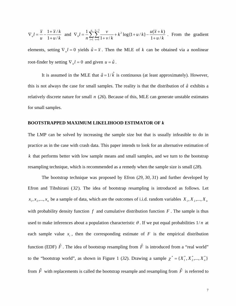
elements, setting 0=∇ lu yields u x= . Then the MLE of k can be obtained via a nonlinear

root-finder by setting 0=∇ lk and given uu ˆ= .

It is assumed in the MLE that ˆˆ 1/a k= is continuous (at least approximately). However,

this is not always the case for small samples. The reality is that the distribution of a exhibits a

relatively discrete nature for small n (26). Because of this, MLE can generate unstable estimates

for small samples.

BOOTSTRAPPED MAXIMUM LIKELIHOOD ESTIMATOR OF k

The LMP can be solved by increasing the sample size but that is usually infeasible to do in

practice as in the case with crash data. This paper intends to look for an alternative estimation of

k that performs better with low sample means and small samples, and we turn to the bootstrap

resampling technique, which is recommended as a remedy when the sample size is small (28).

The bootstrap technique was proposed by Efron (29, 30, 31) and further developed by

Efron and Tibshirani (32). The idea of bootstrap resampling is introduced as follows. Let

nxxx ,...,, 21 be a sample of data, which are the outcomes of i.i.d. random variables nXXX ,...,, 21

with probability density function f and cumulative distribution function F . The sample is thus

used to make inferences about a population characteristic θ . If we put equal probabilities n/1 at

each sample value ix , then the corresponding estimate of F is the empirical distribution

function (EDF) F . The idea of bootstrap resampling from F is introduced from a “real world”

to the “bootstrap world”, as shown in Figure 1 (32). Drawing a sample },...,,{ **2

*1

*nXXX=χ

from F with replacements is called the bootstrap resample and resampling from F is referred to

8

as the nonparametric bootstrap. In reality, a large number of resamples, such as 200 or more,

need to be drawn to achieve robust estimates of inferences. In this way, the distribution of θ can

be approximated by the distribution of *θ .

The bootstrap has several good features in dealing with small sample problems. First,

unlike the classic procedures, the bootstrap does not rely on theoretical distributions and thus

does not require strong assumptions of the sample and the distribution. This is a nice attribute

since it is usually difficult to obtain accurate parameters for a certain distribution given small

samples. Moreover, by bootstrapping, the original sample is duplicated many times. Hence, the

bootstrap can treat a small sample as the virtual population and generate more observations from

it. Finally, the bootstrap is a rather simple technique and does not require a sophisticated

mathematical background for people to use it. Because of those strengths, the bootstrap

techniques have been widely applied to many engineering areas and applications, including radar

and sonar signal processing, geophysics, biomedical engineering, imaging processing, control,

and environmental engineering(33). The bootstrap techniques are widely used for estimating

statistical features including bias (34, 35), variance (36, 37), hypothesis testing (38, 39), and

confidence interval (40, 41).

The proposed BMLE method to estimate the fixed k values of negative binomial

distributions under low sample mean and small sample size conditions has the maximum

likelihood estimation nested inside. The BMLE algorithm is shown in the following steps:

Step 1: Data collection. Collect data into 1 2{ , ,..., }nX X Xχ = , then construct the

empirical distribution function F , which puts equal mass 1/ n at each observation:

1 1 2 2 n n, X = x , ..., X = xX x= .

9

Step 2: Resampling. Draw a random sample of size n with replacements from F :

* * *1 2* { , ,..., }nX X Xχ = . Calculate the variance and mean of the resample *χ . If the variance is

less than or equal to the mean, redraw *χ .

Step 3: Calculation of the bootstrap estimate. Calculate the bootstrap estimate of *k from

*χ using the maximum likelihood method.

Step 4: Iteration. Repeat steps 2 and 3 B times to obtain b estimates of *k :

* * *1, 2, ,, ,...,b b b bk k k .

Step 5: Estimation of k . Sort the b estimates of *k , then k is approximated by the

median value of * * *1, 2, ,, ,...,b b b bk k k .

In step 5, the median value is used instead of the mean as the estimate of k because the

median value is less sensitive to the skewness of the distribution of * * *1, 2, ,, ,...,b b b bk k k .

SIMULATIONS AND RESULTS

Monte Carlo simulations are conducted to show the performance and applicability of the BMLE

under low sample mean and small sample size situations. Also, estimated results from MME,

MLE, and BMLE are compared to investigate their relative performances. The simulation

procedure is as follows.

Step 1: Generate a sample 1 2{ , ,..., }nX X Xχ = with size n from the negative binomial

distribution ~ ( , )X NB u k . Calculate the variance and mean of the sample, regenerate χ if the

variance to mean value is less than or equal to 1.

10

Step 2: Calculate the estimate of k from χ , using MME, MLE, and BMLE respectively.

For the BMLE, a fixed number of resampling 499B = is used (500 samples counting the

original one).

Step 3: Repeat steps 1 and 2 until r estimates of k are obtained.

In the simulations, wide but practical ranges of the parameters are considered as follows:

u : 0.75, 1, 1.5, and 2 respectively.

k : 1, 2, 3, and 4 for each u .

n : may take values of 20, 50, 100, 200, 500, and 1000, and varies according to

the performances of those three estimators.

r : 1000 times.

During the simulation, a sample was discarded if an estimate failed to converge. As in the

study by Wilson et al. (11), we set upper and lower limits of 1000 and 0.001 on the dispersion

parameter for the MLE. Thus, estimates by the MLE that exceed the upper and lower limits are

discarded, and corresponding estimates by the MME and BMLE are also removed. Those

estimates are not counted in r .

Simulations were realized through the Matlab software, which provides both the

resampling and the maximum likelihood algorithms. Other software programs such as SAS,

GenStat, and Rgui can also be used for such work. Simulation results are shown in Tables 1

through 4 with different parameter settings. k values in the tables are set to 1, 2, 3, and 4

sequentially. Bias, variance, and the Mean Square Error (MSE) of estimates from r simulation

runs are used for comparing the performances of the three estimators. The bias measures the

difference between the true value and the average of all estimates ( kkEkbias −= ]ˆ[)ˆ( ); the

11

variance measures the spread of the estimates about the mean of all estimates

( ]])ˆ[ˆ[( 22ˆ kEkEk

−=σ ); and the MSE is calculated by 2ˆ

2))ˆ((k

kbiasMSE σ+= .

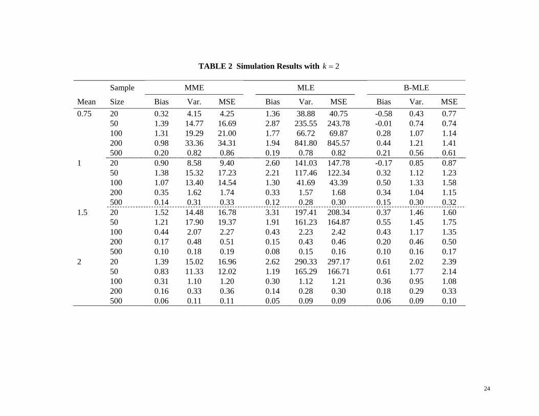
It is interesting to note that the performances of those estimators not only depend on the

sample mean and sample size, but also rely highly on the k value. Through comparing the four

tables, it can be seen that with a fixed sample mean and a fixed sample size, the increase of k

deteriorates estimation performances as shown by the increasing values for bias, variance, and

MSE from table to table, especially for the MME and the MLE. This agrees with Willison’s (11)

and Lord’s (42) conclusions. When the k value is low, for example, 1k = , for 1u = , the MME

and the MLE can have relatively accurate estimations when the sample size is as low as 100

(MSEs of 0.48 and 0.42 for MME and MLE, respectively). While with 4k = , the sample size

has to be more than 1000 to obtain reasonably stable and accurate estimations. At sample size of

500, MSEs are still as large as 18.80 and 20.71 for MME and MLE, respectively. The BMLE, on

the other hand has superior estimates. Even when 4k = ( 1u = ), it can still deliver relatively

accurate and stable estimations for the sample size of 100, with a very good MSE at only 2.26,

comparing with MSEs of 62.46 and 396.76 for MME and MLE. To better illustrate the

performances of those three methods, three boxplots of estimates are shown in Figure 2, with

1 ,4 == uk and 200n = . From the figure, while the three boxplots have almost identical median

values around 4, the boxplot of the BMLE has the shortest inter-quartile range (IQR), the range

between the 25th and the 75th percentiles ( 13 QQIQR −= ), indicated by the shorter box. Outliers

of the BMLE, as defined as those that are beyond IQRQ *5.13 + , are much closer to the median

value and they are much fewer in number as compared with MME and MLE. Note that some

outliers in the boxplots of the MME and the MLE are not displayed since they are further out

from the median value and clear differences in performances have already been displayed.

12

Tables 1 through 4 also show that generally the MME has smaller bias and variance than

the MLE with relatively small samples. This agrees with the conclusion stated by Pieters et al.

(43). The MME is also less likely to have large overestimations. Only at large sample sizes, the

MLE is slightly better than the MME and about the same as the BMLE. This demonstrates that

the MLE is only suitable for large samples, but may still be unstable under low mean and high k

conditions. The BMLE outperforms the MME in all sample size scenarios. It also outperforms

the MLE in almost all cases except a few in which the sample sizes are very large. For those

limited number of cases the performance of the BMLE is about the same as that of the MLE. The

tables clearly show that the BMLE is much more robust in estimating k under low sample mean

conditions. The BMLE does need more expensive computations, but with the development of

modern computing capabilities this problem can be almost neglected.

APPLICATION WITH OBSERVED CRASH DATA

A crash count dataset is used as an example to show different performances of the three

estimators. The sample dataset was collected from 4-legged unsignalized intersections in

Toronto, Ontario (44), with the initial objective of developing statistical models for predicting

safety performance of these intersections. It was later used to fit negative binomial models (4).

Fatal and non-fatal injuries are included in this dataset. There are 354 observations, and the

sample has a mean value of 1 and a variance-to-mean of 1.28. The maximum and minimum

values of this sample are 5 and 0, respectively. Like in Lord’s study (4), we assume no spatial or

temporal correlation between those observations for simplicity and use the dataset to examine the

effects of low sample means and small sample sizes on different estimators. By randomly

selecting observations from the dataset, we can obtain subsamples with different sample sizes.

13

The three estimators were firstly used to estimate the k parameter for the full dataset.

Then, the full dataset was treated as the sample population and subsamples were generated from

it. 1000 subsamples, with sample sizes of 50, 100, and 200 respectively, were generated. These

subsamples were drawn with overdispersion ( xs >2 ) to fit negative binomial distributions. The

k values were estimated by the three estimators. Results of the statistics are shown in Table 5.

For sample sizes of 50, 100, and 200, the mean values in Table 5 are averages of estimation from

1000 subsamples. For the BMLE method, 499 resamples are drawn from each subsample.

For the full dataset, all the estimated k values are between 3 and 4, suggesting the k

value should be somewhere between 3 and 4. The estimated k values from the MLE and BMLE

are close, which is a conclusion similar to one reached from simulations with large sample size

and also suggesting the k value should be around 3.3. For the subsamples with different smaller

sample sizes, it is again found that both the MME and the MLE are unstable with large

estimation variance while the BMLE has small variance of estimation. From Tables 3 and 4, it

can be inferred that with a k value between 3 and 4 and 1=u , the BMLE tends to slightly

underestimate k with the fixed sample size of 50, and slightly overestimate k with the fixed

sample size of 200, while the other two estimators tend to overestimate the k value by a larger

margin under both scenarios. These phenomena seem to be very well identified by this example:

the MME and MLE estimated k at values from 4.55 to 6.38, significantly high than the 3 to 4

range; while for the BMLE it seemed to underestimate k at 2.95 with sample size of 50 and

slightly overestimate it at 3.85 with the sample size of 200. Table 5 again shows that the BMLE

produces more accurate estimations and also with much smaller spread when sample sizes are

small. Table 5 results also show the good stability of the BMLE method as the estimated mean

and variance do not differ too much for different sample sizes.

14

CONCLUSIONS

Crash count data for safety analysis tend to display the character of overdispersion and

the negative binomial distribution is widely used as the model to fit the data. In practice, crash

count data are often characterized by low sample mean values and small sample sizes, which

make accurate and robust estimation of the dispersion parameter difficult to achieve using the

most common methods.

To improve the estimation of the dispersion parameter for data with low sample mean

and small sample sizes, this paper proposed a new method, the bootstrapped maximum

likelihood estimate, which combines the maximum likelihood method with the bootstrapping

resampling technique. Various Monte Carlo simulations of the negative binomial distributions

with low sample means are conducted, and the results show that the proposed estimator produces

the most accurate and stable estimates. In the end, the superiority of the proposed estimator is

demonstrated using observed crash count dataset.

This research only focuses on estimation of the dispersion parameter of the negative

binomial distribution. Further work should be conducted to expand the proposed bootstrapped

maximum likelihood estimate for negative binomial regression models that include covariates.

15

REFERENCE

1 Nicholson, A., and Y. Wong. Are Accidents Poisson distributed? A Statistical Test. Accident

Analysis and Prevention, Vol.25, No. 1, pp. 91-97, 1993.

2 Bliss, C.I., and R.A. Fisher. Fitting the Negative Binomial Distribution to Biological Data

and Not on the Efficient Fitting of the Negative Binomial. Biometrics 9, pp. 176-200, 1953.

3 Poch, M., and F.L. Mannering. Negative Binomial Analysis of Intersection Accident

Frequency. Journal of Transportation Engineering, Vol. 122, No. 2, pp.105-113, 1996.

4 Lord, D. Modeling Motor Vehicle Crashes using Poisson-Gamma Models: Examining the

Effects of Low Sample Mean Values and Small Sample Size on the Estimation of the Fixed

Dispersion Parameter. Accident Analysis & Prevention, Vol. 38, No. 4, pp. 751-766, 2006.

5 Hauer, E. Observational Before-After Studies in Road Safety: Estimating the Effect of

Highway and Traffic Engineering Measures on Road Safety. Oxford, England: Pergamon

Press, Elsevier Science Ltd, 1997.

6 Washington, S.P., M.G. Karlaftis, and F.L. Mannering. Statistical and Econometric Methods

for Transportation Data Analysis. Chapman & Hall CRC, 2003.

7 Taylor, L.R. Aggregation, Variance, and the Mean. Nature189, pp. 732-735, 1961.

8 Bliss, C.I., and A.R.G. Owen. Negative Binomial Distributions with a Common k.

Biometrika, Vol. 45, No. 1/2, pp. 37-58, 1958.

9 Fisher, R.A. The Negative Binomial Distribution. Annals of Eugenics 11, pp. 182-187, 1941.

10 Neyman, J. On a New Class of ‘Contagious’ Distributions, Applicable in Entomology and

Bacteriology. Annals of Mathematical Statistics 10, pp. 35-57, 1939.

11 Willson, L.J., J.L. Folks, and J.H. Young. Multistage Compared with Fixed-Sample-Size

Estimation of the Negative Binomial Parameter k. Biometrics, Vol. 109-117, 1984.

16

12 Bliss, C.I., and A.R.G. Owen. Negative Binomial Distributions with a Common k.

Biometrika, Vol. 45, No. ½, pp. 37-58, 1958.

13 Anscombe, F.J. Sampling Theory of the Negative Binomial and Logarithmic Series

Distributions. Biometrika 37, pp.358-382, 1950.

14 Wood, G.R. Confidence and Prediction Intervals for Generalized Linear Accident Models.

Accident Analysis & Prevention, Vol. 37, No. 2, pp. 267-273, 2005.

15 Hauer, E. Overdispersion in Modelling Accidents on Road Sections and in Empirical Bayes

Estimation. Accident Analysis & Prevention, Vol. 33, No. 6, pp. 799-808, 2001.

16 Persaud, B., and C. Lyon. Empirical Bayes before–after safety studies: Lessons learned from

two decades of experience and future directions. Accident Analysis & Prevention, 2006, in

press.

17 Anscombe, F.J. The Statistical Analysis of Insect Counts Based on the Negative Binomial

Distributions. Biometrics 5, pp. 165-173, 1949.

18 Lawless, J.F. Negative Binomial and Mixed Poisson Regression. The Canadian Journal of

Statistics 15, pp. 209-225, 1987.

19 Clark, S.J., and J.N. Perry. Estimation of the Negative Binomial Parameter k by Maximum

Quasi-Likelihood. Biometrics 45, pp. 309-316, 1989.

20 Maycock, G., and R.D. Hall. Accidents at 4-Arm Roundabouts. TRRL Laboratory Report

1129. Transportation and Road Research Laboratory, Crowthorne, Bershire, 1984.

21 Fridstrom, L.J.I., S. Ingebrigtsen, S.R. Kulmala, and L.K. Thomsen. Measuring the

Contribution of Randomness, Exposure, Weather, and Daylight to the Variation in Road

Accident Counts. Accident Analysis and Prevention, Vol. 27, No. 1, pp. 1-20, 1995.

17

22 Maher, M.J., and I. Summersgill. A Comprehensive Methodology for the Fitting Predictive

Accident Models. Accident Analysis and Prevention, Vol. 28, No. 3, pp. 281-296, 1996.

23 Kumara, S.S.P., H.C. Chin, and W.M.S.B. Weerakoon. Identification of Accident Causal

Factors and Prediction of Hazardousness of Intersection Approaches. Transportation

Research Record 1840, pp. 116- 122, 2003.

24 Oh, J., C. Lyon, S.P. Washington, B.N. Persaud, and J. Bared. Validation of the FHWA Crash

Models for Rural Intersections: Lessons Learned. Transportation Research Record 1840, pp.

41-49, 2003.

25 Lord, D., and J.A. Bonneson. Calibration of Predictive Models for Estimating the Safety of

Ramp Design Configurations. Transportation Research Record 1908, pp. 88-95, 2005.

26 Piegorsch, W.W. Maximum Likelihood Estimation for the Negative Binomial Dispersion

Parameter. Biometrics 46, pp. 863-867, 1990.

27 Toft, N., G.T. Innocent, D.J. Mellor, and S.W.J. Reid. The Gamma-Poisson Model as a

Statistical Method to Determine if Micro-Organisms are Randomly Distributed in a Food

Matrix. Food Microbiology, Vol. 23, No. 1, pp. 90-94, 2006.

28 Diaconis, P., and B. Efron. Computer-intensive Methods in Statistics. Scientific American, pp.

116-130, 1983.

29 Efron, B. Bootstrap Methods: Another Look at the Jackknife. The Annals of Statistics 7, pp.

1-26, 1979.

30 Efron, B. Nonparametric Estimates of Standard Error: The Jackknife, the Bootstrap and

Other Methods. Biometrika 63, pp.589-599, 1981.

31 Efron, B. The Jackknife, the Bootstrap, and Other Resampling Plans. Society of Industrial and

Applied Mathematics CBMS-NSF Monographs 38, 1982.

18

32 Efron, B., and R.J. Tibshirani. An Introduction to the Bootstrap. New York: Chapman & Hall,

1993.

33 Zoubir, A.M., and D.R. Iskander. Bootstrap Techniques for Signal Processing. Cambridge

University Press, 2004.

34 Politis, D.N. Computer-Intensive Methods in Statistical Analysis. IEEE Signal Processing

Magazine 15, pp. 39-55, 1998.

35 Tamstorf, R., and H.W. Jensen. Adaptive Sampling And Bias Estimation in Path Tracing. In

“Rendering Techniques’97.” Eds. J. Dorsey and Ph. Slusallek. Springer-Verlag. Pp. 285-295,

1997.

36 Rosychuk, R., X. Sheng, and J.L. Stuber. Comparison of Variance Estimation Approaches in

a Two-State Markov Model for Longitudinal Data with Misclassification. Statistics in

Medicine, Vol. 25, No. 11, pp. 1906-1921, 2006.

37 Yeo, D, H. Mantel, and T.P.Liu. Bootstrap Variance Estimation for the National Population

Health Survey. Proceedings of the Annual Meeting of the American Statistical Association,

Survey Research Methods Section, August 1999. Baltimore: American Statistical

Association, 1999.

38 Zoubir, A. M. Multiple Bootstrap Tests and Their Application. In Proceedings of the IEEE

International Conference on Acoustics, Speech and Signal Processing (ICASSP) VI, pp. 69-

72, Adelaide, Australia, April 1994.

39 Hall, P., S.R. Wilson. Two Guidelines for Bootstrap Hypothesis Testing. Biometrics 47, pp.

757-762, 1991.

40 Fisher, N.I., and P. Hall. Bootstrap Confidence Regions for Directional Data. Journal of the

American Statistical Society 84, pp. 996-1002, 1989.

19

41 Reid, D.C., A.M. Zoubir, and B. Boashash. The Bootstrap Applied to Passive Acoustic

Aircraft Parameter Estimation. In: Proceedings ICASSP '96, Atlanta, pp. 3154～3157, 1996.

42 Lord, D., and L.F. Miranda-Moreno. Effects of Low Sample Mean Values and Small Sample

Size on the Estimation of the Fixed Dispersion Parameter of Poisson-gamma Models for

Modeling Motor Vehicle Crashes: A Bayesian Perspective. Presented at the 86th Annual

Meeting of the Transportation Research Board, Washington, D.C., 2006.

43 Pieters, E.G., C.E. Gates, J.H. Matis, and W.L. Sterling. Small Sample Comparisons of

Different Estimators of Negative Binomial Parameters. Biometrics 33, pp. 718-723, 1977.

44 Lord, D. The Prediction of Accidents on Digital Networks: Characteristics and Issues Related

to the Application of Accident Prediction Models. Ph.D. Dissertation, Department of Civil

Engineering, University of Toronto, Toronto, Ontario, 2000.

20

LIST OF FIGURES

FIGURE 1 The bootstrap approach (Efron and Tibshirani, 1993). ................................. 21

FIGURE 2 Boxplot of estimates with 1 ,4 == uk and 200n = ..................................... 22

LIST OF TABLES

TABLE 1 Simulation Results with 1k = .......................................................................... 23

TABLE 2 Simulation Results with 2k = ........................................................................ 24

TABLE 3 Simulation Results with 3k = ......................................................................... 25

TABLE 4 Simulation Results with 4k = ......................................................................... 26

TABLE 5 Estimation Results of the k Parameter for Crash Count Data ........................ 27

21

FIGURE 1 The bootstrap approach (Efron and Tibshirani, 1993).

22

FIGURE 2 Boxplots of estimates with 1 ,4 == uk and 200n = .

23

TABLE 1 Simulation Results with 1k =

MME MLE BMLE

Mean Sample Size Bias Var. MSE Bias Var. MSE Bias Var. MSE

0.75 20 0.69 2.60 3.09 1.11 17.78 19.01 0.14 0.39 0.41 50 0.88 7.70 8.47 1.55 110.69 113.1 0.28 0.46 0.54 100 0.26 0.82 0.89 0.23 0.97 1.02 0.21 0.30 0.34 200 0.14 0.21 0.23 0.11 0.18 0.19 0.13 0.18 0.20 1 20 0.85 3.86 4.58 1.34 23.91 25.70 0.30 0.56 0.65 50 0.59 3.36 3.71 0.64 14.33 14.74 0.36 0.51 0.63 100 0.21 0.43 0.48 0.18 0.39 0.42 0.20 0.26 0.31 200 0.09 0.12 0.13 0.07 0.09 0.10 0.09 0.10 0.11 1.5 20 0.76 3.53 4.11 1.05 27.81 28.91 0.43 0.68 0.86 50 0.35 2.35 2.48 0.43 31.99 32.17 0.28 0.43 0.51 100 0.14 0.16 0.18 0.11 0.13 0.14 0.14 0.14 0.16 200 0.06 0.07 0.07 0.05 0.05 0.05 0.06 0.05 0.06 2 20 0.69 3.22 3.69 0.76 7.81 8.39 0.52 0.94 1.21 50 0.22 0.41 0.46 0.17 0.34 0.37 0.22 0.33 0.38 100 0.12 0.11 0.13 0.09 0.09 0.09 0.11 0.09 0.11 200 0.05 0.05 0.05 0.03 0.04 0.04 0.04 0.04 0.04

24

TABLE 2 Simulation Results with 2k =

Sample MME MLE B-MLE

Mean Size Bias Var. MSE Bias Var. MSE Bias Var. MSE 0.75 20 0.32 4.15 4.25 1.36 38.88 40.75 -0.58 0.43 0.77 50 1.39 14.77 16.69 2.87 235.55 243.78 -0.01 0.74 0.74 100 1.31 19.29 21.00 1.77 66.72 69.87 0.28 1.07 1.14 200 0.98 33.36 34.31 1.94 841.80 845.57 0.44 1.21 1.41 500 0.20 0.82 0.86 0.19 0.78 0.82 0.21 0.56 0.61 1 20 0.90 8.58 9.40 2.60 141.03 147.78 -0.17 0.85 0.87 50 1.38 15.32 17.23 2.21 117.46 122.34 0.32 1.12 1.23 100 1.07 13.40 14.54 1.30 41.69 43.39 0.50 1.33 1.58 200 0.35 1.62 1.74 0.33 1.57 1.68 0.34 1.04 1.15 500 0.14 0.31 0.33 0.12 0.28 0.30 0.15 0.30 0.32 1.5 20 1.52 14.48 16.78 3.31 197.41 208.34 0.37 1.46 1.60 50 1.21 17.90 19.37 1.91 161.23 164.87 0.55 1.45 1.75 100 0.44 2.07 2.27 0.43 2.23 2.42 0.43 1.17 1.35 200 0.17 0.48 0.51 0.15 0.43 0.46 0.20 0.46 0.50 500 0.10 0.18 0.19 0.08 0.15 0.16 0.10 0.16 0.17 2 20 1.39 15.02 16.96 2.62 290.33 297.17 0.61 2.02 2.39 50 0.83 11.33 12.02 1.19 165.29 166.71 0.61 1.77 2.14 100 0.31 1.10 1.20 0.30 1.12 1.21 0.36 0.95 1.08 200 0.16 0.33 0.36 0.14 0.28 0.30 0.18 0.29 0.33 500 0.06 0.11 0.11 0.05 0.09 0.09 0.06 0.09 0.10

25

TABLE 3 Simulation Results with 3k =

Sample MME MLE BMLE

Mean Size Bias Var. MSE Bias Var. MSE Bias Var. MSE 0.75 50 1.30 22.25 23.95 3.69 434.12 447.72 -0.68 0.86 1.32 100 2.24 51.12 56.12 4.16 387.81 405.11 -0.07 1.34 1.35 200 1.82 44.85 48.15 2.33 106.92 112.34 0.35 1.89 2.01 500 0.66 16.94 17.37 0.72 30.20 30.72 0.45 2.05 2.26 1000 0.26 1.11 1.18 0.27 1.07 1.15 0.30 1.04 1.13 1 50 1.61 26.19 28.79 3.48 797.57 809.66 -0.16 1.23 1.26 100 1.95 33.32 37.14 2.77 127.68 135.36 0.44 2.08 2.27 200 0.93 11.23 12.09 0.98 12.86 13.83 0.54 2.27 2.55 500 0.37 2.24 2.38 0.38 2.34 2.48 0.39 1.61 1.76 1000 0.14 0.46 0.48 0.14 0.44 0.46 0.17 0.45 0.48 1.5 50 2.12 37.55 42.03 3.77 343.90 358.08 0.56 2.63 2.94 100 1.29 23.20 24.86 1.54 51.16 53.52 0.74 2.97 3.51 200 0.49 3.27 3.52 0.50 3.32 3.57 0.51 2.20 2.47 500 0.19 0.64 0.67 0.18 0.60 0.63 0.22 0.62 0.67 2 50 2.06 46.27 50.50 3.35 275.58 286.80 0.92 3.62 4.47 100 0.80 7.84 8.47 0.80 10.03 10.68 0.71 2.77 3.28 200 0.31 1.27 1.37 0.31 1.22 1.31 0.38 1.28 1.43 500 0.11 0.36 0.38 0.10 0.34 0.35 0.13 0.34 0.36

26

TABLE 4 Simulation Results with 4k =

Sample MME MLE BMLE

Mean Size Bias Var. MSE Bias Var. MSE Bias Var. MSE 0.75 50 0.80 23.04 23.69 3.45 407.23 419.14 -1.55 0.85 3.25 100 2.29 58.11 63.37 4.37 334.35 353.48 -0.70 1.40 1.89 200 2.98 120.02 128.89 5.18 829.51 856.37 0.00 2.25 2.25 500 1.94 91.61 95.37 2.31 213.92 219.25 0.62 3.63 4.01 1000 0.66 12.19 12.63 0.69 14.00 14.47 0.54 3.02 3.31 1 50 1.46 28.49 30.62 3.58 319.03 331.84 -0.85 1.46 2.18 100 2.26 57.34 62.46 3.82 382.18 396.76 -0.12 2.25 2.26 200 2.41 82.98 88.77 3.17 236.82 246.88 0.50 3.30 3.55 500 0.82 18.14 18.80 0.84 20.00 20.71 0.60 3.46 3.82 1000 0.33 1.86 1.97 0.34 1.84 1.95 0.37 1.81 1.94 1.5 50 2.40 61.00 66.76 7.40 2828.00 2882.76 0.10 2.70 2.71 100 2.46 71.07 77.13 3.64 264.57 277.79 0.73 4.06 4.59 200 1.31 55.52 57.23 1.80 425.10 428.36 0.78 4.48 5.08 500 0.28 1.73 1.81 0.28 1.64 1.71 0.34 1.68 1.80 1000 0.17 0.67 0.70 0.17 0.64 0.67 0.20 0.66 0.70 2 50 2.60 52.54 59.30 4.33 617.93 636.68 0.74 4.17 4.71 100 1.91 61.97 65.62 2.64 307.03 314.00 0.93 4.96 5.83 200 0.83 8.16 8.85 0.85 8.66 9.38 0.81 4.06 4.72 500 0.21 1.11 1.16 0.22 1.08 1.12 0.27 1.12 1.19 1000 0.08 0.38 0.38 0.09 0.39 0.39 0.11 0.42 0.43

27

TABLE 5 Estimation Results of k for Crash Count Data

sample MME MLE BMLE

size Mean Var. Mean Var. Mean Var.

354* 3.78 3.26 3.35 50** 5.15 26.99 6.38 238.55 2.95 1.49 100** 5.64 38.49 5.77 90.82 3.57 2.36 200** 4.98 22.88 4.55 30.56 3.85 2.68

Note: *: one dataset is used. **: 1000 subsamples are used.