estimating the cost of capital implied by market prices and accounting...

Foundations and Trends R© inAccountingVol. 2, No. 4 (2007) 241–364c© 2009 P. Easton

DOI: 10.1561/1400000009

Estimating the Cost of Capital Implied byMarket Prices and Accounting Data∗

Peter Easton

Center for Accounting Research and Education, The University of NotreDame, Notre Dame, Indiana 46556-5646, [email protected]

Abstract

Estimating the Cost of Capital Implied by Market Prices andAccounting Data focuses on estimating the expected rate of returnimplied by market prices, summary accounting numbers, and forecastsof earnings and dividends. Estimates of the expected rate of return,often used as proxies for the cost of capital, are obtained by invertingaccounting-based valuation models. The author describes accounting-based valuation models and discusses how these models have been used,and how they may be used, to obtain estimates of the cost of capital.

* I thank Brad Badertscher, Matt Brewer, Devin Dunn, Gus De Franco, Vicki Dickinson,Cindy Durtschi, Pengjie Gao, Joost Impiink, Lorie Marsh, Steve Monahan, Jim Ohlson,Steve Orpurt, Ken Peasnell, Stephen Penman, Greg Sommers, Jens Stephan, Gary Taylor,Laurence van Lent, Arnt Verriest, Xiao-Jun Zhang, PhD. students in the Limperg InstituteAdvanced Capital Markets course at Tilburg University, and participants at the Universityof Cincinnati 4th Annual Accounting Research Symposium, and cost of capital seminarsat the National University of Singapore and Seoul National University, for very helpfuldiscussions as I was writing this survey. Most of all, I thank Bob Lindner, for his clear andfirm guidance very early in my career; this survey reflects that guidance.

1

Introduction

The focus of this survey is on estimating the expected rate of returnimplied by market prices, summary accounting numbers (such as bookvalue and earnings), and forecasts of earnings and dividends. Estimatesof the expected rate of return, which are often used as proxies for thecost of capital, are obtained by inverting accounting-based valuationmodels. I begin by describing accounting-based valuation models andthen I discuss the way these models have been used, and how they maybe used, to obtain estimates of the cost of capital.

The re-introduction of the residual income valuation model byOhlson (1995) and the development of the abnormal growth in earningsmodel by Ohlson and Juettner-Nauroth (2005) have been the driv-ing force behind the burgeoning empirical literature that reverse engi-neers these models to infer markets expectations of the rate of returnon equity capital. The obvious advantage of this reverse-engineeringapproach is that estimates of the expected rate of return are basedon forecasts rather than extrapolation from historical data. Prior tothe development of these approaches, researchers and valuation practi-tioners relied on estimates based on historical data (estimated via themarket model, the empirical analogue of the Sharpe–Lintner Capital

242

243

Asset Pricing Model, or variants of the Fama and French (1992)three/four-factor model). As a practical matter the usefulness of theseestimates is very limited. Fama and French (1997, 2002) concludethat these estimates, based on historical return data are “unavoidablyimprecise” and empirical problems “probably invalidate their use inapplications.”

The practical appeal of accounting-based valuation models, partic-ularly the abnormal growth in earnings model, is that they focus onthe two variables that are most commonly at the heart of valuationscarried out by practicing equity analysts; namely, forecasts of earningsand forecasts of earnings growth. The question at the core of this surveyis: How can these forecasts be used to obtain an estimate of the costof capital? After addressing this question, I will examine the empiricalvalidity of the estimates based on these forecasts and then I will explorepossible means of improving these estimates.

The later part of the survey details a method for isolating the effectof any factor of interest (such as cross-listing, fraud, disclosure quality,taxes, analyst following, accounting standards, etc.) on the cost ofcapital.1

If you are interested in understanding the key ingredients of theacademic literature on accounting-based estimates of expected rate ofreturn this survey is for you. My aim is to provide a foundation fora deeper comprehension of this literature and to give a jump start tothose who may have an interest in extending this literature.

I have deliberately chosen to introduce the key ideas via examplesbased on actual forecasts, accounting information, and market prices forlisted firms. I have found that people exposed to this literature for thefirst time find this a useful way to gain a sound intuitive understandingof the essential elements of the models and methods. I then show howthe numerical examples are based on sound algebraic relations.2

1 I do not review the large literature that examines the effect of various factors on the costof capital. This literature developed very shortly after the first accounting based empiricalestimates of the cost of capital were developed. I expect that the reader of this surveymay conclude that many of these studies should be re-visited after more refined estimatesof the cost of capital have been developed.

2Many readers of this survey have observed that these numerical examples have been criticalto their understanding. Some have underscored the importance of these examples when

244 Introduction

The survey proceeds as follows:

Section 2: Valuing the firm

The survey begins by reviewing, in Section 2, the discounted cashflow valuation model and the closely related accounting-based valu-ation model; namely, the residual operating income valuation model.These models are used to value the operations of the firm. I have chosento use the discounted cash flow valuation model as the starting pointbecause most readers have at least some familiarity with the use of thisvaluation model.

The theoretical papers that underpin this survey are, by and large,based on the dividend capitalization model, which is a model of equityvaluation, rather a model for the valuation of the firm. The keypapers are Ohlson (1995) and Ohlson and Juettner-Nauroth (2005).The empirical literature has also focused on the valuation of equity. Mysense is that this emphasis is primarily driven by the availability of data.The models used in the valuation of equity are discussed in Sections 3and 4. I will discuss the related empirical literature in the later sections.There is still a great deal of room for research that focuses on the oper-ations of the firm rather than the portion of those assets that are ownedby equity shareholders. I return to this point at the end of the survey.

I demonstrate valuation of the firm in Section 2 by means of a simpleexample similar to those used in introductory accounting and financecourses.3 In this example, there are forecasts of free cash flow fromoperations for the next four years, together with forecasts of expectedgrowth beyond this four-year horizon. The forecasted free cash flows arediscounted to determine the present value of the firm, which is oftenreferred to as the enterprise value. Other terms used include firm value,asset value, and value of operations.

Next, I illustrate the residual operating income valuation modelusing the same example. Again, the focus is on valuing the operations.I show, through the example, that free cash flow from operations is

telling me that they have undertaken the exercise of setting up the related spreadsheetsand repeating the calculations; this ensures a thorough understanding of the valuationmodels because all of the algebraic relations are implicit in the set up of the spreadsheets.

3The example is the same as that in Easton et al. (2008).

245

equal to net operating profit after taxes (NOPAT) adjusted for theaccrual components, which may also be referred to as non cash-flowcomponents, of operating income. I use this equality to show how theresidual operating income valuation model is derived from the free cashflow valuation model.

Section 3: Changing the focus to the valuation of equity and introducingreverse engineering

The structure of Section 3 closely parallels Section 2. Focus is shiftedfrom valuation of the firm to valuation of equity. Most of the remain-ing sections focus on valuing equity and, in turn, on calculating theimplied expected rate of return on equity capital. The parallels betweenSections 2 and 3 should be borne in mind when reading the remainder ofthe survey. I begin Section 3 by introducing the dividend capitalizationmodel from which I derive the residual income valuation model. Theparallels between: (1) the valuation of the firm based on the discountedcash flow valuation model and the valuation of equity based on thedividend capitalization model; and (2) the derivation of the residualoperating income valuation model from the discounted cash flow valu-ation model and the derivation of the residual income model from thedividend capitalization model, become apparent.

This survey is on estimating the cost of capital implied by marketprices and accounting data. The empirical literature that estimates thecost of capital based on market prices and accounting data reverseengineers the accounting-based valuation models to obtain estimatesof the implied expected rate of return, which, in turn is used as aproxy for the cost of capital. The concept of reverse engineering isintroduced at the end of Section 3. Reverse engineering to obtain theimplied expected rate of return depends critically on the maintainedassumption about the growth rate beyond the period for which forecastsare available. The effect of the growth-rate assumption on estimates ofthe implied expected rate of return becomes evident in the example.

Although the term cost of capital is commonly used to describethe implied expected rates of return, they are not the cost of cap-ital unless the market prices are efficient and the earnings forecastsare the market’s earnings expectations. A more precise term would be

246 Introduction

“the internal rate of return implied by market prices, accounting bookvalues and analysts’ forecasts of earnings.” Since many of the earningsforecasts used in the extant literature are made by analysts who arein the business of making stock buy/sell recommendations, estimatesof the expected rate of return implied by these analysts’ forecasts andmarket prices are, arguably, not estimates of the cost of capital. Itwould seem reasonable to suggest, for example, that analysts may basetheir recommendations on the difference between the internal rate ofreturn implied by market prices, accounting book values and analysts’forecasts of earnings and the cost of equity capital.

Section 4: Reverse engineering the abnormal growth in earnings valua-tion model: PE ratios and PEG ratiosThe residual income valuation model anchors the valuation of equityon book value of equity and makes adjustments to this valuation viafuture expected residual income. The abnormal growth in earningsmodel, which is also derived from the dividend capitalization model,anchors the valuation of equity on capitalized future earnings and thenmakes adjustments to this value via future expected abnormal growthin earnings.

In Section 4, I derive and illustrate the abnormal growth in earningsvaluation model, focusing on the meaning of abnormal growth inearnings. Reverse engineering the abnormal growth in earnings valu-ation model to obtain estimates of the expected rate of return andexpected growth beyond the earnings forecast horizon is also illus-trated. Valuations based on the price-earnings (PE) ratio and on thePEG ratio (the PE ratio divided by short-term earnings growth) arespecial cases of the abnormal growth in earnings valuation model. Ishow in Section 4 that reverse engineering these ratios to obtain esti-mates of the expected rate of return may rely on assumptions thatare not descriptively valid. I illustrate modifications that may improvethese estimates of the expected rate of return.

Section 5: Reverse-engineering accounting-based valuation models toobtain firm-specific estimates of the implied expected rate of return

Section 5 focuses on reverse engineering the residual income valuationmodel and the abnormal growth in earnings valuation model to obtain

247

firm-specific estimates of the implied expected rate of return on equity,which, in turn, may be used as estimates of the cost of equity capital.I present a critical assessment of the most commonly used reverse-engineering methods.

Sections 6 and 7: Reverse engineering the valuation models to obtainportfolio-level estimates of the implied expected rate of return

Section 6 describes methods of reverse engineering the abnormalgrowth in earnings valuation model to obtain portfolio-level estimatesof the implied expected rate of return. Section 7 describes two methodsfor reverse engineering the residual income valuation model to obtainportfolio-level estimates of the expected rate of return. The clearadvantage of these methods is that they simultaneously estimatethe expected rate of return and the expected growth rate impliedby the data. Estimating both of these rates avoids the need formaking inevitably erroneous assumptions about the expected growthrate beyond the earnings forecast horizon. The growth rates are theexpected rate of change in abnormal growth in earnings and theexpected residual income growth rate.

Section 8: Methods for assessing the quality/validity of firm-specificestimates

Section 8 describes and evaluates two approaches to assessing the valid-ity/reliability of firm-specific estimates of the expected rate of returnon equity capital. The first method asks: Do the estimates of ex anteexpected return explain ex post realized return? The second method,which is more common in the literature, asks: What is the correlationbetween the estimates of the expected rate of return and commonlyused risk proxies? I show that the second method has serious shortcom-ings and conclude that the method that relies on explanatory power forex post realized returns, after controlling for omitted correlated vari-ables, is the best extant method for evaluation of the estimates.

Section 9: Measurement error in firm-specific estimates of the expectedrate of return

Section 9 focuses on the firm-specific estimates of the implied expectedrate of return in the extant literature and summarizes results of

248 Introduction

analyses of their quality and validity. Unfortunately, the news is bad;the firm-specific estimates are quite poor, and thus unreliable. I has-ten to add, however, that this is not a reason to abandon the use ofthese estimates. The lack of reliability is a reflection of the fact that theresearch literature is in its infancy; there are significant opportunitiesfor research that has the aim of improving these estimates. Section 11provides some suggestions.

Section 10: Bias in estimates of the expected rate of return due to biasin earnings forecasts

Evidence of bias, that is systematic or nonzero average error, in esti-mates of the implied expected rate of return is presented and discussedin this section. This evidence complements the evidence of error at thefirm-specific level discussed in Section 9.

Section 11: Dealing with shortcomings in firm-specific estimates

Section 11 suggests ways of dealing with the shortcomings in firm-specific estimates of the implied expected rate of return and ways ofmitigating the effects of bias in portfolio-level estimates. Possible direc-tions for future research are also discussed.

Section 12: Methods for determining the effect of a phenomenon ofinterest on the cost of capital

Much of the research literature asks the question: What is the effectof a phenomenon of interest (for example, disclosure quality, cross-listing, adoption of IFRS) on the cost of equity capital? Section 12describes a method for determining these effects. The method comparesestimates of the implied expected rate of return among groups of stocks,which differ in the phenomenon of interest. The method also permitsintroduction of control variables to deal with differences among thegroups of stocks.

Section 13: Data Issues

Section 13 describes data issues that are often, in fact usually, encoun-tered when estimating rates of return implied by accounting data andmarket prices. These issues are often overlooked even though they maybe important as a practical matter. Ways of dealing with these issues

249

are discussed. The main focus is on developing a method that facili-tates daily estimation of the implied expected rate of return using onlypublicly available information at the estimation date.

Section 14: Some thoughts on future directions

Section 14 provides a brief summary and speculates on possibledirections for future research.

2

Valuing the Firm

The next three sections of the survey lay out the basic elements of thevaluation models that have been reverse-engineered to obtain estimatesof the cost of capital. Since the emphasis of this survey is on the esti-mates of the cost of capital rather than on the valuation models per se,my discussion of these models is brief. Details of the derivations of thesemodels, of the properties of these models, and of their relative strengthsand weaknesses as practical valuation tools may be found elsewhere;see, for example, Ohlson and Gao (2006) and Penman (2007).

I have chosen to begin this survey with a discussion of the discountedcash flow valuation model for two reasons. First, the discounted cashflow valuation model is familiar to most people who have an interest inestimates of the cost of capital. Often the reason for this interest is theneed to obtain an estimate of the discount rate to be used to estimatethe present value of a series of cash flow forecasts. Second, the approachof “undoing” the accounting accruals to obtain an estimate of the freecash flow from forecasts of earnings, which is often taught in financeclasses, may be turned on its head to show that the accounting-basedvaluation models are readily derived from this discounted cash flowmodel.

250

251

After laying out the basic ingredients of the discounted cash flowvaluation model, I discuss an example based on forecasts for Procterand Gamble Inc. (P&G). In this example, there are forecasts of free cashflow from operations for the next four years, together with forecastsof expected growth in free cash flow beyond this four year horizon;these forecasts of free cash flow and growth are derived from forecastedincome statement and balance sheet data. The forecasted free cash flowsare discounted using the weighted average cost of capital as the discountrate to determine the present value of the firm (usually referred to asthe enterprise value).

I also introduce the residual operating income valuation model inthis section and I illustrate its use with the P&G example. Again, thefocus is on valuing the firm rather than valuing the equity. I show, bymeans of the example, that free cash flow from operations is equal tonet operating profit after taxes (NOPAT) adjusted for the accrual com-ponents, which may also be referred to as non-cash-flow components, ofoperating income. It follows that a variant of the free cash flow valua-tion model that focuses on operating income minus a capital charge forthe investment in operations, that is, residual operating income, maybe derived. I illustrate this residual operating income valuation modelusing the P&G example.

Since the focus of this survey is on reverse-engineering accounting-based valuation models to obtain estimates of the cost of capital,I illustrate the fundamental idea behind these estimates by reverse-engineering the residual operating income valuation model with theP&G data. Rather than calculating an intrinsic value of P&G, I deter-mine the internal rate of return that is implied by P&G’s market valueand the forecasts of NOPAT. This internal rate of return may be viewedas the market’s expected rate of return on P&G, and, in turn, it maybe viewed as an estimate of the cost of capital for P&G.

At the outset, it is important to repeat the point made in the intro-duction that using this internal rate of return as an estimate of the costof capital implicitly assumes that the market prices are efficient andthat the operating income forecasts capture the market’s expectations.It is important to bear in mind that these assumptions may not bevalid.

252 Valuing the Firm

The P&G example illustrates the equivalence of the discountedcash flow valuation model and the residual operating income valuationmodel. This equivalence is underscored at the end of the section viaa formal derivation of the residual operating income valuation modelfrom the discounted cash flow valuation model.

2.1 The Discounted Cash Flow Valuation Model

The discounted cash flow (DCF) valuation model may be written asfollows:

V0 =∞∑t=1

(FCFt

(1 + ro)t

), (2.1)

where V0 is the intrinsic (or true economic) value of the operations ofthe firm, FCFt is the after-tax free cash flow from the operations of thefirm in period t, and ro is the expected rate of return on the operationsof the firm.1

As a practical matter, we do not have forecasts for an infiniteperiod. If we have an estimate of the expected growth in free cashflows beyond the forecast horizon (gfcf), we can implement the follow-ing finite-horizon version of the DCF valuation model2:

V0 =T−1∑t=1

(FCFt

(1 + ro)t

)+(

FCFT

(ro − gfcf) ∗ (1 + ro)T−1

)(2.2)

1This expected rate of return on operations is often referred to as the cost of capital forthe firm and, as a practical matter, is often determined as the weighted average of theafter-tax cost of debt and the cost of equity capital; referred to as the weighted averagecost of capital (WACC).

2This form of the model implicitly assumes that the cash flow grows at gfcf duringyear T . If the infinite growth rate begins for year T + 1, the model must be written asfollows:

V0 =T∑

t=1

(FCFt

(1 + ro)t

)+

(FCFT (1 + gfcf)

(ro − gfcf) ∗ (1 + ro)T

).

2.2 A Simple Example 253

2.2 A Simple Example

I use forecasts for P&G to illustrate discounted cash flow valuation.These forecasts are based on a careful review of the financial statementsand some knowledge of the company’s plans. I use P&G’s 2006 incomestatement and balance sheet as the basis for the forecasts3:

Sales $68,222Sales growth rate 4.4%Net operating profit before tax $13,249Net operating profit after tax (NOPAT) $9,221Net operating assets (NOA) $99,879Net operating profit margin (NOPM) ($9,221/$68,222) 13.52%Net operating asset turnover (NOAT) ($68,222/$99,879) 0.683

Using these inputs, I forecast P&G’s sales, NOPAT and NOA.4

Each year’s forecasted sales is the prior year sales multiplied succes-sively by (one-plus) the expected sales growth rate, or 1.044 in thiscase, and then rounded to whole digits. NOPAT is computed usingforecasted (and rounded) sales each year times the 2006 net operatingprofit margin (NOPM) of 13.52%; and NOA is computed using fore-casted (and rounded) sales divided by the 2006 net operating assetturnover (NOAT) of 0.683.5 Forecasted numbers for 2007 through 2010are provided in the following table.

3P&G’s fiscal year ended on June 30, 2006. In this example, “years” are fiscal years. Com-paring P&G sales for 2005 and 2006, we see a 20.2% increase ([$68,222/$56,741] − 1).This sales growth is high and I question its persistence. Further analysis reveals P&G’s2006 sales include eight months of sales from Gillette after its acquisition by P&G during2006. P&G’s 2005 sales do not include those from Gillette. Thus, comparing 2005 to 2006is not valid. Footnotes reveal pro forma sales that show what the income statement wouldhave reported had Gillette’s full-year sales been included in both 2005 and 2006; P&G’ssales growth would have been 4.4%, which is more realistic, and is the forecasted salesgrowth I use.

4NOPAT is sales less operating expenses (including the effect of taxes), NOA is current andlong-term operating assets less current and long-term operating liabilities; or operatingworking capital plus long-term net operating assets.

5NOPM is the ratio of NOPAT to sales; NOAT is the ratio of sales to net operating assets.


Procter & Gamble Multiyear Forecasts of Sales,

NOPAT and NOA ($millions)

2006 2007 Est. 2008 Est.

Net sales $68,222 $71,224 $74,358

($68,222 × 1.044) ($71,224 × 1.044)

NOPAT $9,221 $9,627 $10,051

($71,224 × 13.52%) ($74,358 × 13.52%)

NOA $99,879 $104,274 $108,862

($71,224/0.683) ($74,358/0.683)

2009 Est. 2010 Est.

Net sales $77,629 $81,045

($74,358 × 1.044) ($77,629 × 1.044)

NOPAT $10,493 $10,955

($77,629 × 13.52%) ($81,045 × 13.52%)

NOA $113,652 $118,652

($77,629/0.683) ($81,045/0.683)

These forecasts of NOPAT and NOA may be used to obtain forecastsof FCF; which is equal to NOPAT minus the change in net operatingassets. Note that this is, in fact, the standard calculation seen in mostvaluation texts where change in net operating assets is broken intoseveral main components; such as change in working capital (changein inventory, change in accounts receivable, and change in accountspayable), depreciation, and capital expenditure.6

For the sake of the example, assume a growth rate beyond the four-year forecast horizon of 4.4%, and a cost of capital for operations (alsoreferred to as the weighted average cost of capital) of 7%.7 The calcu-lation of free cash flow and the valuation based on the discounted cashflow valuation model are provided in the following table.

6Another way of understanding this calculation is to note that we are adjusting NOPATfor the accounting accruals to get to a free cash flow number; note that NOPAT containsaccruals such as change in receivables, change in payables, change in inventory, etc. andchange in NOA also contains these same items so that it follows that NOPAT minus changein NOA is equal to free cash flow.

7The weighted average cost of capital for P&G of 7% was obtained from Bloomberg onJune 30, 2006.

2.3 The Residual Operating Income Valuation Model 255

YearTerminal

(In millions) 2006 2007 2008 2009 2010 yearSales $68,222 $71,224 $74,358 $77,629 $81,045 $84,611NOPAT 9,221 9,627 10,051 10,493 10,955 11,437NOA 99,879 104,274 108,862 113,652 118,652 123,873Increase 4,394 4,588 4,790 5,001 5,221

in NOAFCF 5,232 5,463 5,703 5,954 6,216

V0 =5,2321.07

+5,4631.072

+5,7031.073

+5,9541.074

+6,216

(0.07 − 0.044) ∗ 1.074

= $201,245.

That is, the estimated intrinsic value of the operations of P&G is$201,245.

2.3 The Residual Operating Income Valuation Model

Notice that in determining the forecasts of free cash flow, we use thefact that:

FCFt = NOPATt − ∆NOAt. (2.3)

Recognizing this fact, we can substitute for FCFt in Equation (2.1) toobtain the residual operating income valuation model8

V0 = NOA0 +∞∑t=1

(NOPATt − roNOAt−1

(1 + ro)t

). (2.4)

And, since we only have forecasts for a finite future period, we imple-ment the finite horizon version of this model:

V0 = NOA0 +T−1∑t=1


(1 + ro)t

)

+(

NOPATT − roNOAT−1

(r − gropi) ∗ (1 + ro)T−1

), (2.5)

8More details of this derivation are provided in Section 2.6.


where gropi is the expected growth in residual operating income beyondthe forecast horizon.

Applying this model to the P&G forecasts, we obtain:

V0 = 99,879 +(9,627 − 0.07 ∗ 99,879)

1.07+

(10,051 − 0.07 ∗ 104,274)1.072

+(10,493 − 0.07 ∗ 108,862)

1.073+

(10,955 − 0.07 ∗ 113,652)1.074

+(11,437 − 0.07 ∗ 118,652)

(0.07 − 0.044) ∗ 1.074

= $201,245.

This value is the same as we obtained using the discounted cash flowvaluation model. This is expected because models (2.1) and (2.4) arelinked by an identity, Equation (2.3). However, in the finite horizon wealso need gfcf to be equal to gropi if we are to obtain the same valuation.This will be so if (as in our P&G example) we have forecasted to thepoint where sales are assumed to be growing at a constant rate (4.4%for P&G) and the NOPM and the NOAT are assumed to be constant.In other words, we have forecasted to “steady-state,” which is oftendone in practice.

2.4 Reverse Engineering

The focus of this survey is on using forecasts of accounting numbers toestimate the cost of capital. I illustrate the fundamental idea behindthese estimates by reverse engineering the residual operating incomevaluation model with the P&G data. Rather than calculating an intrin-sic value of P&G as we have just done, we can determine the internalrate of return that is implied by P&G’s market value and the forecastswe have made. This internal rate of return may be viewed as the mar-ket’s expected rate of return on P&G, and, in turn, it may be viewed asan estimate of the cost of capital for P&G. Note that, since the focusremains on the operations of the firm, we obtain an estimate of the costof capital for operations, which is also called the cost of capital for thefirm or the weighted-average cost of capital. I will return to this point.

2.5 The Algebra of the Accounting-based Valuation Models 257

On July 1, 2006, P&G’s market value was $212,557 million.9 Thismarket value and the forecast of NOPAT and NOA, imply an internalrate of return of 6.86%; which is the solution to the following equation:

212,557 = 99,879 +(9,627 − ro ∗ 99,879)

(1 + ro)+

(10,051 − ro ∗ 104,274)(1 + ro)2

+(10,493 − ro ∗ 108,862)

(1 + ro)3+

(10,955 − ro ∗ 113,652)(1 + ro)4

+(11,437 − ro ∗ 118,652)(ro − 0.044) ∗ (1 + ro)4

That is, our forecasts, taken together with the market price, suggestthat the market expects a return of 6.86% on the operations of P&G;this expected rate of return may be viewed as an estimate of the costof capital for operations.

2.5 The Algebra of the Derivation of the Accounting-basedValuation Models

The algebra of the derivation of the accounting-based valuation modelsis as follows. We will see this algebra in the derivation of the resid-ual operating income model in the next section, in the derivation ofthe residual income model in Section 3, and in the derivation of theabnormal growth in earnings valuation model in Section 4.

The derivation of accounting-based valuation models begins withthe capitalization model:

V =∞∑

t=1

(xt

(1 + r)t

), (2.6)

where xt is the pay-off; either free cash flow if V is the value of thefirm, or dividends (that is, net payments to equity holders) if V is thevalue of equity. The next step is introduction of the following zero-sumequality10:

0 = y0 +y1 − (1 + r)y0

(1 + r)+

y2 − (1 + r)y1

(1 + r)2+ · · · (2.7)

9$35,816 million owned by debt-holders and $176,741 million owned by equity holders(3,178,800,000 shares priced at $55.60 per share).

10 The role of this zero-sum equality is explained in Ohlson and Gao (2006).


this may be more easily understood if re-written as follows:

0 = y0 − y0 +y1

(1 + r)− y1

(1 + r)+

y2

(1 + r)2− y2

(1 + r)2+ · · ·

where yt is a valuation anchor such as book value or capitalized next-period earnings. This zero-sum equality permits the introduction of theaccounting-based valuation anchor to the valuation model.

Adding Equations (2.6) and (2.7) yields:

V = y0 +∞∑t=1

(yt + xt − (1 + r) ∗ yt−1

(1 + r)t

). (2.8)

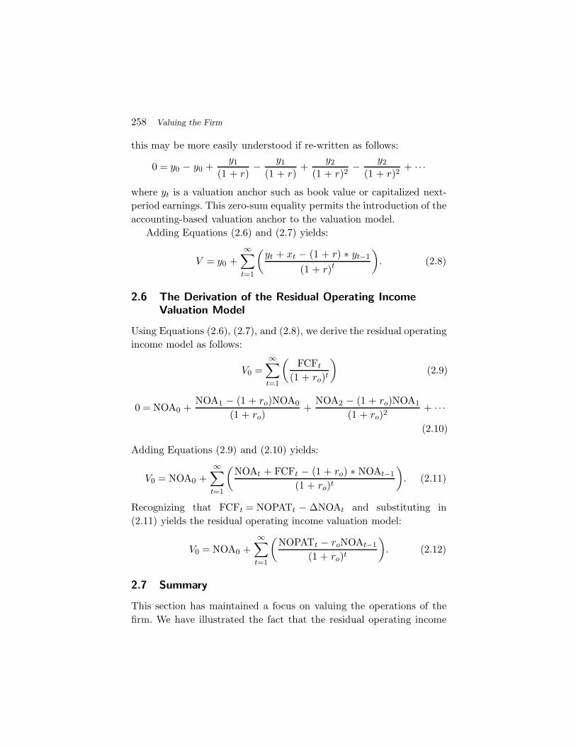
2.6 The Derivation of the Residual Operating IncomeValuation Model

Using Equations (2.6), (2.7), and (2.8), we derive the residual operatingincome model as follows:

V0 =∞∑t=1

(FCFt

(1 + ro)t

)(2.9)

0 = NOA0 +NOA1 − (1 + ro)NOA0

(1 + ro)+

NOA2 − (1 + ro)NOA1

(1 + ro)2+ · · ·(2.10)


V0 = NOA0 +∞∑

t=1

(NOAt + FCFt − (1 + ro) ∗ NOAt−1

(1 + ro)t

). (2.11)

Recognizing that FCFt = NOPATt − ∆NOAt and substituting in(2.11) yields the residual operating income valuation model:

V0 = NOA0 +∞∑t=1


(1 + ro)t

). (2.12)

2.7 Summary

This section has maintained a focus on valuing the operations of thefirm. We have illustrated the fact that the residual operating income

2.7 Summary 259

valuation model may be derived from the discounted cash flow valuationmodel and we have seen that the residual operating income valuationmodel may be reverse-engineered to determine the expected rate ofreturn that is implied by market prices, the book value of net operatingassets, and forecasts of NOPAT.

Although we may be able to make our own forecasts of NOPAT,these forecasts are generally not readily available for large samples ofobservations. On the other hand, forecasts of earnings are readily avail-able and this is the most likely reason why the research literature hastended to focus on reverse-engineering earnings-based valuation modelsrather than models based on NOPAT and free cash flow. The next twosections examine earnings-based valuation models that are at the centerof much of the academic literature.

3

Changing the Focus to the Valuation of Equityand Introducing Reverse Engineering

Professional analysts tend to forecast dividends and earnings.1 For alarge company, like P&G, these forecasts are available from a varietyof sources. For example, ValueLine provided the following forecasts forP&G at the end of June 2006:

year

2007 2008 2009 2010 2011Earnings per share 3.02 3.45 3.83 4.22 4.60Dividends per share 1.41 1.54 1.66 1.78 1.90Price per share 100.00

How can these forecasts be converted into an estimate of the intrinsicvalue of an equity share of P&G? How can these forecasts be used toobtain an estimate of the cost of capital? How might these forecastsbe used as the basis for stock recommendations? I will answer thesequestions in this section.

1Analysts have, more recently been forecasting cash flow numbers; these numbers must beused cautiously as they are likely not free cash flow as defined in Section 2.

260

3.1 The Dividend Capitalization Model 261

I begin Section 3 with a discussion of the dividend capitalizationmodel from which I derive the residual income valuation model. I illus-trate this model using the forecasts for P&G. In the latter part of thesection, I demonstrate reverse engineering of the dividend capitaliza-tion model and the residual income valuation model to obtain estimatesof the cost of equity capital.

The set-up of Section 3 closely parallels that of Section 2. The par-allels between: (1) the valuation of the firm based on the discountedcash flow valuation and the valuation of equity based on the dividendcapitalization model; and (2) the derivation of the residual operatingincome valuation model from the discounted cash flow valuation modeland the derivation of the residual income model from the dividendcapitalization model, become apparent.

This survey is on estimating the cost of capital implied by marketprices and accounting data. The empirical literature that estimates thecost of capital based on market prices and accounting data reverseengineers the accounting-based valuation models to obtain estimatesof the implied expected rate of return, which, in turn is used as aproxy for the cost of capital. The concept of reverse engineering isintroduced at the end of the section. Reverse engineering to obtain theimplied expected rate of return depends critically on the maintainedassumption about the growth rate beyond the period for which forecastsare available. The effect of the growth-rate assumption on estimates ofthe implied expected rate of return becomes evident in the example.

3.1 The Dividend Capitalization Model

The dividend capitalization model may be written as follows:

V E0 =

∞∑t=1

(dpst

(1 + rE)t

), (3.1)

where V E0 is the intrinsic value of an equity share, dpst is the expected

dividend per share paid to a shareholder of the firm in period t, andrE is the expected rate of return on the equity investment.

Again, as a practical matter, we do not have forecasts for aninfinite period. If, instead, we have estimates of the expected growth in

262 Focus on the Valuation of Equity and Introducing Reverse Engineering

dividends beyond the investment horizon (gd), we can implement thefollowing finite-horizon version of the dividend capitalization model:

V E0 =

T∑t=1

(dpst

(1 + rE)t

)+(

dpsT (1 + gd)(rE − gd) ∗ (1 + rE)T

)(3.2)

and if we have a forecast of share prices at the end of the forecasthorizon, as we do for P&G, we can invoke the following form of themodel:

V E0 =

T∑t=1

(dpst

(1 + rE)t

)+(

priceT

(1 + rE)T

). (3.3)


Applying the dividend capitalization model to the forecasts for P&Gwe obtain:

V E0 =

1.411.079

+1.54

1.0792+

1.661.0793

+1.78

1.0794+

1.901.0795

+100

1.0795

= $74.94

(in this illustrative example, I use Bloomberg’s estimate of the cost ofequity capital for P&G, which was 7.9% at the end of June 2006).

That is, ValueLine’s forecasts of dividends and terminal price, andBloomberg’s estimate of the cost of equity capital, suggest that P&G’smarket price of $55.60 at the date of these forecasts was too low.

Rather than using Bloomberg’s estimate of the cost of equitycapital, we can reverse engineer the dividend capitalization model todetermine the implied market expected rate of return. Continuing withthe P&G example, we solve the following equation:

55.60 =1.41

(1 + rE)+

1.54(1 + rE)2

+1.66

(1 + rE)3+

1.78(1 + rE)4

+1.90

(1 + rE)5+

100(1 + rE)5

rE = 9.05%.

3.3 The Residual Income Valuation Model 263

That is, analysts’ forecasts of dividends and terminal prices implythat they expect a return of 9.05% on an equity investment in P&G.

Also, to illustrate the use of Equation (3.2), let us suppose that wedid not have a forecast of price for P&G at the end of the forecasthorizon. Then the unknown would be growth in dividends beyond theinvestment horizon (gd). We can reverse engineer the dividend capital-ization model to obtain an estimate of this growth rate:

55.60 =1.411.079

+1.54

1.0792+

1.661.0793

+1.78

1.0794+

1.901.0795

+1.90(1 + gd)

(0.079 − gd) ∗ (1.079)5

gd = 5.1%.

3.3 The Residual Income Valuation Model

The residual income valuation model relies on the accounting stocksand flows equation; sometimes referred to as the clean-surplus relation.This equation simply states that value at the beginning of the period,reported on the balance sheet as the book value of common shareholderequity (bpst−1), plus the value created during the period, reported onthe income statement as net income (epst), minus the value distributedduring the period, in the form of dividends (dpst), is the value at theend of the period (bpst). That is

bpst = bpst−1 + epst − dpst

or,

dpst = epst − ∆bpst. (3.4)

Recognizing this fact, we can substitute for dpst in the dividend capital-ization model, Equation (3.1), to obtain the residual income valuationmodel2:

V E0 = bps0 +

∞∑t=1

(epst − rEbpst−1

(1 + rE)t

). (3.5)

2See Section 3.6 for a formal derivation.


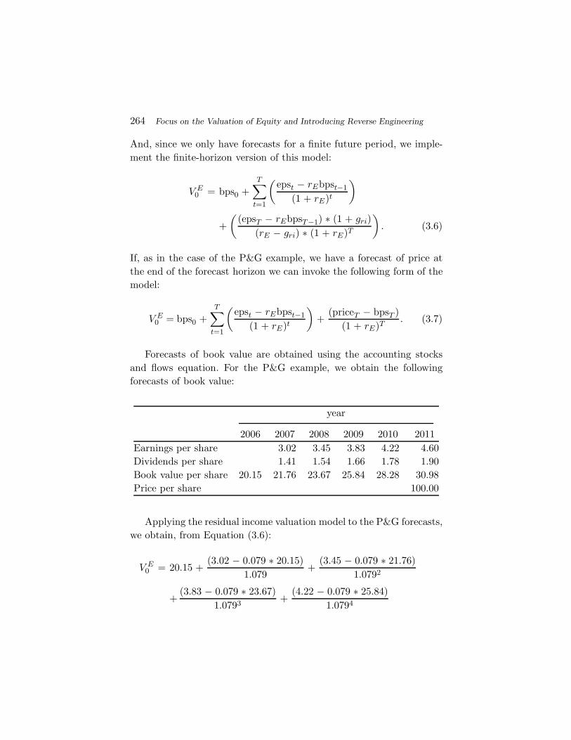
And, since we only have forecasts for a finite future period, we imple-ment the finite-horizon version of this model:

V E0 = bps0 +

T∑t=1


(1 + rE)t

)

+(

(epsT − rEbpsT−1) ∗ (1 + gri)(rE − gri) ∗ (1 + rE)T

). (3.6)

If, as in the case of the P&G example, we have a forecast of price atthe end of the forecast horizon we can invoke the following form of themodel:

V E0 = bps0 +

T∑t=1


(1 + rE)t

)+

(priceT − bpsT )(1 + rE)T

. (3.7)

Forecasts of book value are obtained using the accounting stocksand flows equation. For the P&G example, we obtain the followingforecasts of book value:

year

2006 2007 2008 2009 2010 2011Earnings per share 3.02 3.45 3.83 4.22 4.60Dividends per share 1.41 1.54 1.66 1.78 1.90Book value per share 20.15 21.76 23.67 25.84 28.28 30.98Price per share 100.00

Applying the residual income valuation model to the P&G forecasts,we obtain, from Equation (3.6):

V E0 = 20.15 +

(3.02 − 0.079 ∗ 20.15)1.079

+(3.45 − 0.079 ∗ 21.76)

1.0792

+(3.83 − 0.079 ∗ 23.67)

1.0793+

(4.22 − 0.079 ∗ 25.84)1.0794

3.4 Reverse Engineering the Residual Income Valuation Model 265

+(4.60 − 0.079 ∗ 28.28)

1.0795+

(4.60 − 0.079 ∗ 28.28) ∗ 1.04324(0.079 − 0.04324) ∗ 1.0795

= $74.94.

and from Equation (3.7):

V E0 = 20.15 +

(3.02 − 0.079 ∗ 20.15)1.079

+(3.45 − 0.079 ∗ 21.76)

1.0792

+(3.83 − 0.079 ∗ 23.67)

1.0793+

(4.22 − 0.079 ∗ 25.84)1.0794

+(4.60 − 0.079 ∗ 28.28)

1.0795+

(100 − 30.98)1.0795

= $74.94.

Notice that we have reverse engineered the residual income modelto obtain a growth rate gri = 4.324%. The present value of residualincome growing perpetually beyond the five-year forecast horizon at4.324% from the 2011 base ($4.60 − 0.079 ∗ $28.28) will be equal tothe 2011 difference between the forecasted price ($100) and expectedbook value ($30.98).

3.4 Reverse Engineering the Residual IncomeValuation Model

Rather than calculating an intrinsic value of P&G, we can determinethe internal rate of return that is implied by P&G’s market price andthe ValueLine forecasts. This internal rate of return may be viewed asthe market’s expected rate of return on P&G, and, in turn, it may beviewed as an estimate of the cost of capital for P&G. Since the focusnow is on the equity ownership of P&G, this internal rate of return isan estimate of the cost of equity capital.

The price of P&G stock at the date of the forecasts in this examplewas $55.60. This stock price, the forecasts of earnings, and a rate ofgrowth in residual income of 4.324% beyond 2011, imply an internal


rate of return of 9.05%, which is the solution to the following equation:

55.60 = 20.15 +(3.02 − rE ∗ 20.15)

(1 + rE)+

(3.45 − rE ∗ 21.76)(1 + rE)2

+(3.83 − rE ∗ 23.67)

(1 + rE)3+

(4.22 − rE ∗ 25.84)(1 + rE)4

+(4.60 − rE ∗ 28.28)

(1 + rE)5+

(4.60 − rE ∗ 28.28) ∗ 1.04324(rE − 0.04324) ∗ (1 + rE)5

.

In other words, the ValueLine forecasts, taken together with the marketprice, suggest an expected rate of return of 9.05% on equity investmentin P&G. This rate is higher than the Bloomberg estimate, probablyreflecting optimism in the ValueLine forecasts. We will return to thispoint in Sections 8 and 9.

Recall that the growth rate of 4.324% beyond 2011 was based onthe ValueLine 2011 price per share forecast of $100; which may be quiteoptimistic. Observe, alternatively, that we can take the Bloomberg esti-mate of the cost of equity capital (7.9%) as given, and reverse engineerthe residual income valuation model, to obtain the implied expectedrate of growth in residual income:

55.60 =20.15 + (3.02 − 0.079 ∗ 20.15)

1.079+

(3.45 − 0.079 ∗ 21.76)(1.079)2

+(3.83 − 0.079 ∗ 23.67)

(1.079)3+

(4.22 − 0.079 ∗ 25.84)(1.079)4

+(4.60 − 7.9% ∗ 28.28)

(1.079)5+

(4.60 − 0.079 ∗ 28.28) ∗ (1 + gri)(0.079 − gri) ∗ (1.079)5

gri = 1.98%.

3.5 The Importance of Simultaneously EstimatingBoth the Implied Expected Rate of Return andthe Implied Expected Growth Rate

The example in Section 3.4 illustrates the interdependence of the esti-mate of the expected rate of return and the estimate of the expectedrate of growth. The assumption about one of these expectations affects

3.6 Formal Derivation of the Residual Income Valuation Model 267

the estimate of the other, and vice versa. This underscores the needfor a method that reverse engineers this valuation model to simultane-ously estimate both the implied expected rate of return and the impliedexpected growth rate. This method will be detailed in Section 9.

3.6 Formal Derivation of the Residual Income ValuationModel

We derive the residual income model as follows:

V E0 =

∞∑t=1

(dpst

(1 + rE)t

)(3.8)

0 = bps0 +bps1 − (1 + rE)bps0

(1 + rE)+

bps2 − (1 + rE)bps1(1 + rE)2

+ · · · (3.9)


V E0 = bps0 +

∞∑t=1

(bpst + dpst − (1 + rE) ∗ bpst−1

(1 + rE)t

). (3.10)

Recognizing dpst = epst − ∆bpst and substituting in (3.9) yields theresidual income valuation model:

V E0 = bps0 +

∞∑t=1


(1 + rE)t

). (3.11)

3.7 The Importance of the Clean-Surplus Assumption

I have shown the derivation of the residual income valuation model on aper share basis. Of course, one could also derive the model following thesame steps to obtain the total dollar value of equity. As Ohlson (2005)points out, future equity transactions that are expected to change thenumber of shares outstanding generally imply that the clean-surplusassumption does not hold on a per share basis. Many studies haveignored this issue and calculated forecasted book value by assumingthat the clean-surplus assumption holds; the effect of this assumptionon the validity of the implied expected rate of return obtained in thesepapers is unknown. Ohlson (2005) further observes that for the residual


income valuation model to hold on a total dollar basis, issuances andre-purchases of shares must be value-neutral from the point of view ofnew, future shareholders; again, the impact of these assumptions onthe validity of implied expected rate of return is unknown.

These concerns lead Ohlson (2005) to advocate the use of the abnor-mal earnings growth valuation model discussed in the next section. It isimportant to note, however, that there are sound reasons for advocatingthe use of the extant empirical methods for obtaining estimates of theimplied expected rate of return that are based on the residual incomevaluation model rather than the extant methods based on the abnor-mal growth in earnings valuation model. These reasons are discussedlater in the survey.

3.8 Summary

This section has changed the focus from the valuation of the opera-tions of the firm and reverse-engineering the residual operating incomevaluation model to obtain an estimate of the cost of capital for opera-tions to a focus on the valuation of equity and reverse engineering theresidual income model to obtain an estimate of the cost of equity cap-ital. The residual income valuation model is derived from the dividendcapitalization model. And, the importance of assumptions about theexpected rate of growth beyond the earnings forecast horizon is illus-trated. In the next section, another equity valuation model, based onearnings and earnings growth rather than on book value and residualincome will be illustrated and derived.

4

Reverse Engineering the Abnormal Growth inEarnings Valuation Model: PE Ratios and

PEG Ratios

The residual income valuation model discussed in Section 3 anchorsthe valuation of equity on book value of equity and makes adjustmentsto this valuation via future expected residual income. The abnormalgrowth in earnings model, which is also derived from the dividend cap-italization model, anchors the valuation of equity on capitalized futureearnings; it then makes adjustments to this value via future expectedabnormal growth in earnings. This model is derived and illustrated inthis section. The derivation is a somewhat over-simplified version ofthe derivation in Ohlson and Juettner-Nauroth (2005) and Ohlson andGao (2006). The reader interested in the detailed derivation and theproperties of this valuation model may fill in the details by readingthese papers.

Valuations based on the price-earnings (PE) ratio and on the PEGratio (the PE ratio divided by short-term earnings growth) are shownin this section to be special cases of the abnormal growth in earningsvaluation model. I show that reverse engineering these ratios to obtainestimates of the expected rate of return may rely on assumptions thatare not descriptively valid. I illustrate modifications that may improvethese estimates of the expected rate of return.

269

270 Abnormal Growth in Earnings Valuation Model: PE Ratios and PEG Ratios

4.1 The Abnormal Growth in Earnings Valuation Model

Forecasts of book value are required to implement the residual incomevaluation model. Although our P&G example suggests that these fore-casts are relatively easy to obtain via forecasts of earnings and divi-dends, this may not always be the case. Also, the obvious focus by theinvestment community on earnings motivates a valuation model basedonly on earnings forecasts. This model is referred to as the AbnormalGrowth in Earnings Valuation Model.

4.2 Formal Derivation of the Abnormal Growth in EarningsValuation Model

The derivation of the abnormal growth in earnings valuation modelfollows the steps outlined via Equations (2.6), (2.7), and (2.8), withdividends as the payoff and capitalized next-period earnings as thevaluation anchor:

V E0 =

∞∑t=1

(dpst

(1 + rE)t

)(4.1)

0 =eps1rE

+eps2rE

− (1 + rE) eps1rE

(1 + rE)+

eps3rE

− (1 + rE) eps2rE

(1 + rE)2+ · · · (4.2)


V E0 =

eps1rE

+∞∑t=1

( epst+1

rE+ dpst − (1 + rE) ∗ epst

rE

(1 + rtE)

). (4.3)

Rearranging yields:

V E0 =

eps1rE

+∞∑

t=2

(epst + rEdpst−1 − (1 + rE) ∗ epst−1

rE ∗ (1 + rE)t−1

)

=eps1rE

+∞∑

t=2

(agrt

rE ∗ (1 + rE)t−1

)(4.4)

where agrt is the abnormal growth in earnings for year t. I will discussthe interpretation of this variable in Section 4.4.

4.3 The Abnormal Growth in EVM and RIVM 271

4.3 The Connection Between the Abnormal Growth inEarnings Valuation Model and the Residual IncomeValuation Model

Notice that the derivation of the abnormal growth in earnings modeldoes not require clean-surplus accounting, thus avoiding the concernsraised by Ohlson (2005), which were outlined in Section 3.7. Ohlson(2005) shows that the residual income valuation model implies theabnormal earnings growth valuation; but the converse does not apply.In other words, the abnormal growth in earnings valuation model is“more robust” from a theoretical viewpoint.1 However, we will see laterthat extant empirical estimates of the implied rate of return obtainedfrom the residual income valuation model are likely to be more robustempirically than those obtained by reverse engineering the abnormalgrowth in earnings valuation model.


In order to apply the abnormal growth in earnings valuation model toa set of finite horizon earnings forecasts, the model may be re-writtenin the following form:

V E0 =

eps1rE

+T∑

t=2

(agrt

rE ∗ (1 + rE)t−1

)

+(

agrT (1 + gagr)(rE − gagr) ∗ rE ∗ (1 + rE)T−1

)(4.5)

and the calculations for P&G are as follows:

year

2007 2008 2009 2010 2011Earnings per share 3.02 3.45 3.83 4.22 4.60Dividends per share 1.41 1.54 1.66 1.78 1.90Abnormal Growth in Earnings 0.30 0.23 0.22 0.19

1See Proposition III in Ohlson (2005).


P&G’s abnormal growth in earnings for 2008 is calculated as: $3.45 +0.079 ∗ ($1.41) − 1.079 ∗ ($3.02) = $0.30. The calculation for otheryears is similar. The intrinsic value of a share of P&G stock is esti-mated as follows:

V E0 =

3.020.079

+0.30

0.079 ∗ 1.079+

0.230.079 ∗ 1.0792

+0.22

0.079 ∗ 1.0793

+0.19

0.079 ∗ 1.0794+

0.19 ∗ 1.01271(0.079 − 0.01271) ∗ 0.079 ∗ 1.0794

= $74.94.

Note that this valuation assumes a rate of change in abnormal growthin earnings beyond the five-year forecast horizon (gagr) of 1.271%, whichis the rate such that the intrinsic value remains at $74.94, which wasthe valuation based on the residual income model. In other words, theabnormal growth in earnings valuation model was reverse engineeredto obtain this growth rate.

4.5 What is Abnormal Growth in Earnings?

For the sake of illustration, suppose we only had earnings forecasts fortwo future periods. We could employ these forecasts to value P&G usingthe following, two-period, version of the abnormal growth in earningsvaluation model:

V E0 =

eps1rE

+agr2

(rE − gagr) ∗ rE. (4.6)

Just as we reverse engineered the residual income valuation modelto obtain an estimate of the cost of equity capital, we can reverseengineer the abnormal growth in earnings valuation model to obtainan estimate of this cost of capital. On the other hand, we could acceptBloomberg’s estimate of the cost of equity capital and reverse engineerthe abnormal growth in earnings model to obtain an estimate of themarket’s expectation of gagr as follows:

55.60 =3.020.079

+0.30

(0.079 − gagr) ∗ 0.079

gagr = −14.2%

4.6 The Concept of Economic Earnings 273

What does this negative 14.2% growth rate mean?2 Before answeringthis question, let us first step back and examine the meaning of agr2008for P&G.

P&G’s abnormal growth in earnings from 2007 to 2008 is forecastto be: $3.45 + 0.079 ∗ ($1.41) − 1.079 ∗ ($3.02) = $0.30. Reverse engi-neering the abnormal growth in earnings valuation model to obtain thechange in the abnormal growth in earnings (beyond 2008) that equatesa price of $55.60, capitalized earnings of $3.02

0.079 and the 2008 abnormalgrowth in earnings of $0.30 yields a change in the abnormal growth inearnings of negative 14.2%. The abnormal growth in earnings of $0.30and the growth from this base at negative 14.2%, are a consequence ofGAAP. To see this, we introduce the concept of economic earnings.

4.6 The Concept of Economic Earnings

With an expected rate of return of 7.9%, P&G’s expected cum-dividendprice at the end of 2007 will be $55.60 ∗ 1.079, or $59.99.3 Economicearnings for 2007 are expected to be $59.99 − $55.60, or $4.39. After$1.41 of dividends, price per share will drop to $58.58. By the end of2008, price is expected to increase to $58.58 ∗ 1.079, or $63.21. That is,economic earnings for 2008 are expected to be $4.63.

If accountants were to record economic earnings instead ofaccounting earnings for P&G, there would be no abnormal growthin earnings ($4.63 + 0.079 ∗ $1.41 − 1.079 ∗ $4.39 = $0.00) for 2008.In this scenario, growth in economic earnings is “normal” inasmuchas cum-dividend earnings grow from 2007 to 2008 at a rate of

2Ohlson and Jeuttner-Nauroth (2005) show that the long-run rate of change in abnormalgrowth in earnings must be positive and less that the cost of capital. But their modeldoes not permit the empirical possibility that the abnormal growth in earnings base onwhich this growth is built may be so high that future (short-run) growth must be negativein order to justify the market price. It is important to note that, although a long-rungrowth rate that is positive and less than the cost of capital is a necessary regularitycondition, the growth rate that is implicit in versions of this model based on earnings forshort forecast horizons is the average of a short-term growth rate (in the P&G examplea short-term attenuation in the abnormal growth in earnings) and the very long-termgrowth rate captured by Ohlson and Jeuttner-Nauroth (2005). Easton (2004) shows thatempirical estimates of gagr are often negative.

3The Bloomberg estimate of the cost of equity capital is chosen for illustrative purposes only.I am not suggesting that Bloomberg’s estimate is either correct or incorrect. This exampleand the examples in the remainder of this section would follow with other estimates.


7.9%.4 But, since accounting earnings differs from economic earn-ings ($3.02 compared with $4.39 in 2007 and $3.45 compared with$4.63 in 2008), there is nonzero abnormal growth in earnings. Inother words, accounting earnings were conservative in 2007; they wereless than economic earnings. The positive ($0.30) abnormal growth inaccounting earnings in 2008 means that accounting earnings partiallyadjust for this conservatism.

4.7 What is Growth in Abnormal Growth in Earnings?

As I have illustrated in Sections 4.4 and 4.5, abnormal growth inearnings is the dollar amount of the difference between cum-dividendearnings in period t ($3.45 + 0.079 ∗ ($1.41) in the P&G example) and“normal earnings,” conditional on earnings of period t − 1 (1.079 ∗($3.02) in the P&G example). The estimate of gagr, which is the esti-mate of the rate of change in abnormal growth in earnings, of negative14.2% is the geometric average rate at which the abnormal growth inearnings of 30 cents will decrease as accounting earnings eventually“correct” for the short-run difference between accounting and eco-nomic earnings in the two-year forecast horizon, 2007 to 2008.5 Thedifference between short-run forecasts of accounting earnings ($3.02and $3.45) and expected economic earnings ($4.39 and $4.63) deter-mines the abnormal growth in earnings agr2008 “base.” The abnormalgrowth in earnings will change from this base at a geometric averagerate gagr of negative 14.2% in the future. As an illustration of the rela-tion between agr2008 and gagr, suppose that the forecast of earnings for2008 includes a nonrecurring item of $0.20. The forecast of earningsif this nonrecurring item had been removed would be $3.25 instead of$3.45. This lower earnings forecast implies a much lower agr2008 ($0.10)and a positive gagr of 0.41%.6

4The “normal” growth in cum-dividend earnings incorporates the dividend irrelevanceproposition of Modiglaini and Miller (1958), which, in essence, implies in this contextthat future dividend payments can be invested at the expected rate of return.

5This growth reflects the fact that differences between accounting earnings and economicearnings in any one period must be captured in accounting earnings of another period (seeEaston et al. (1992) for an elaboration of this point).

6The computations are as follows. agr2008 = 3.25 + 0.079 ∗ 1.41 − 3.02 ∗ 1.079 = 0.10281and from Equation (4.6), 55.6 = 3.02

0.079+ 0.10281

[(0.079−gagr)×0.079], that is, gagr = 0.41%.

4.8 Special Case: PE Ratios 275

4.8 Special Case: PE Ratios

The PE ratio and the PEG ratio, which are often used to comparestocks, are special cases of the two-year abnormal growth in earningsvaluation model:

V E0 =

eps1rE

+agr2

(rE − gagr) ∗ rE. (4.7)

If we assume that agr2 = 0; in other words, if we assume thatnext-year’s forecast of earnings is sufficient for valuation, this relationbecomes:

V E0 =

eps1rE

. (4.8)

In other words, the cost of equity capital may be estimated as theinverse of the forward PE ratio. Reverse engineering this special case ofthe abnormal earnings valuation model would suggest an expected rateof return on equity capital of 5.4% for P&G, which is too low becausethe future accounting earnings growth has been erroneously assumed tobe zero. Investment professionals have observed this shortcoming andsuggested the use of PEG ratios.

4.9 PE Ratios and PEG Ratios

The PEG ratio is equal to the price-earnings ratio divided by anearnings growth rate. Analysts differ in their choice of the form ofthe price-earnings ratio (that is, price-to-trailing earnings or price-to-forward earnings) and in their choice of the earnings growth rate; whichranges from a one-year historical growth rate to an average expectedannual growth rate estimated for several years.

Numerous articles in the popular press describe the pervasive-ness of the use of the PEG ratio as a basis for stock recommen-dations.7 The PEG ratio and its use in valuation is described on

7For example, Barrons (November 9, 1998), Business Week (March 23, 2001), ForbesMagazine (September 2, 2001 and October 28, 2002), New York Times (September 17,2000), Time Magazine (April 1, 2001), and Wall Street Journal (January 24, 2001 andMarch 19, 2001). Financial web sites, (for example, http://www.stockselector.com andhttp://www.fool.com/pegulator) often report PEG ratios and rely on these ratios as aprimary basis for stock recommendations. Bradshaw (2004) further elaborates on theextensive use of the PEG ratio in analysts’ reports.


http://www.fool.com/school/thegrowthrate.htm and is advocated bywell-known Wall Street analyst, Peter Lynch, in his book One Up OnWall Street. The arguments for the use of the PEG ratio vary con-siderably but the essence of these arguments may be summarized asfollows.

Use of the price-to-forward earnings (PE) ratio as a basis for stockrecommendations relies on the notion that, ceteris paribus, a high (low)PE implies a low (high) expected rate of return, supporting a sell (buy)recommendation. However, next period’s earnings may not be indica-tive of the future stream of earnings, and as Lynch ((2000), page 199)observes:

“A company, say, with an [earnings] growth rate of12% a year. . . and a PE ratio of 6 is a very attractiveprospect. On the other hand, a company with a growthrate of 6 percent a year and a PE ratio of 12 is anunattractive prospect and headed for a comedown.”

He goes on to say:

“The PE ratio of any company that’s fairly priced willequal its [earnings] growth rate. . . . In general, a PEratio that’s half the growth rate is very positive, andone that’s twice the growth rate is very negative. Weuse this measure all the time in analyzing stocks formutual funds.”

4.10 Stock Recommendations Based on the PEG Ratio

The comparison of the PE ratio and the earnings growth rate as abasis for stock recommendations is captured in the PEG ratio. Con-sistent with Lynch’s (2000) argument, a stock is fairly priced if itsPEG ratio is equal to one and analysts would recommend holding thestock. A PEG ratio considerably greater/less than one would support asell/buy recommendation. To summarize, the essence of the argumentfor the use of the PEG ratio is that, ceteris paribus, a high (low) PEGimplies that the PE ratio is high (low) relative to the expected rate of

4.11 The Modified PEG Ratio 277

growth in earnings suggesting that the future prospects are expected toworsen (improve), implicitly the expected rate of return is low (high),supporting a sell (buy) recommendation.

Despite the pervasive use of the PEG ratio, its proponents do notprovide a model that is based on fundamental valuation theory. Theabnormal growth in earnings valuation model may be used as this foun-dation/model. We will see this shortly.

4.11 The Modified PEG Ratio

Easton (2004) suggests the following modification to the PEG ratio.Consider the special case gagr = 0.8 That is, agr2 = agr3 = · · · , and thenext period’s expected abnormal growth in earnings provides an unbi-ased estimate of all subsequent periods’ abnormal growth in earnings.This special case of Equation (4.6) may be written9:

P=0

eps2 + rEdps1 − eps1r2E

(4.9)

and

rE =√

eps2 + rEdps1 − eps1P0

. (4.10)

That is:

r2E − rE ∗ dps1

P0− eps2 − eps1

P0= 0. (4.11)

For P&G:

0.1012 − 0.101 ∗ 1.4155.60

− 3.45 − 3.0255.60

= 0.

That is, the implied expected rate of return on equity capital is 10.1%.10

8There will be cases where the assumption gagr = 0 is a very reasonable first approximation.For example, consider Honda Motor Company (HMC), which was trading at a price pershare of $80 at the end of its fiscal year (March 31) 2001. Analysts were forecastingearnings for 2002 and 2003 of $5.50 and $6.25 and dividends of $0.50. If Honda’s expectedrate of return is 10 percent, agr2 = $6.25 + 0.1($0.50) − (1.1)$5.50 = 0.25. In this example,P0 = $80 = [eps1/rE ] + [agr2/r2

E ] = [$5.50/0.1] + [0.25/0.01] and gagr = 0.9We replace intrinsic value V E

0 with market price P0 because we are interested in reverseengineering to determine the expected rate of return implied by this market price.

10 This model is used in several recent studies to estimate an implied expected rate of returnon equity capital (see, for example, Francis et al. (2005) and Hail and Leuz (2006)).


4.12 The PEG Ratio

As a second special case, assume gagr = 0 and dps1 = 0, then fromEquation (4.6):

rE =√

eps2 − eps1P0

. (4.12)

Under these assumptions, the implied estimate of the expected rate ofreturn is equal to the square root of the inverse of the PEG ratio. Tosee this, note that:

(eps2 − eps1)P0

=eps2−eps1

eps1P0

eps1

=1

PEG ∗ 100.

For P&G:

8.8% =

√3.45 − 3.02

55.60.

That is, the implied expected rate of return on equity capital is 8.8%.Notice that this is much lower that the expected rate of return impliedby the modified PEG ratio because the substantial dividends of $1.41are ignored.

4.13 The Gode and Mohanram Modification

Gode and Mohanram (2003) also reverse engineer the abnormal growthin earnings valuation model to obtain estimates of the implied expectedrate of return. They assume that gagr beyond the earnings forecasthorizon is equal to the risk-free rate minus 3%. They also modify theformula for agr2 as follows:

agr2 =eps2 + (1 + ge) ∗ eps1

2+ rEdps1 − (1 + rE) ∗ eps1. (4.13)

The argument for this modification is that the growth in earningsper share from year 1 to year 2 may not be indicative of a long-term

Easton (2004) shows that estimates of the implied expected rate of return based on thismethod are generally biased downward — in other words, the gagr implied by the datais greater than zero.

4.14 Conclusions Regarding Modifications 279

growth. Since analysts also provide an estimate of short-term earningsgrowth rate ge (usually the average rate of growth for years 3 to 5), wemay obtain a more reasonable estimate of the short-term growth rateby taking the average of these two estimates. For the P&G example(where analysts were forecasting a 3 to 5 year growth rate of 11.11%)the Gode and Mohanram (2003) estimate agr2 is:

agr2 =$3.45 + 1.1111 ∗ 3.02

2+ rE$1.41 − (1 + rE) ∗ $3.02.

Their estimate of the implied expected rate of return is the solution to

55.60 =3.02rE

+3.45+1.1111∗3.02

2 + rE ∗ 1.41 − (1 + rE) ∗ 3.02(rE − 0.0171) ∗ rE

.

That is, rE = 9.7%.11

The Gode and Mohanram (2003) modification to the calculation ofagr2 may also be applied to the growth rates used in the calculationof the expected rate of return implied by the PEG ratio and by themodified PEG ratio. The argument against this modification is thatanalysts’ long-term growth rate forecasts tend to be very optimistic;it follows that the implied expected rate of return may be too highrelative to market expectations.

4.14 Conclusions Regarding Modifications

Although the modifications outlined above may serve to improve esti-mates of the expected rate of return on equity capital and facilitatea more meaningful ranking of stocks, these estimates are affected byimplicit or explicit assumptions about growth beyond the forecast hori-zon. This suggests the need for a method that reverse engineers theabnormal growth in earnings valuation model to simultaneously obtainestimates of the expected rate of return and the expected rate ofgrowth. I will describe this method in Section 8.

11 The risk-free rate (return on US Treasury Notes) at the end of 2006 was 4.71%, and hencethe assumed rate of change in abnormal growth in earnings aagr is 1.71%.


4.15 Summary

This section derived and illustrated the abnormal growth in earningsvaluation model and discussed special cases of this model. The conceptof abnormal growth in earnings, which defines short-term earningsgrowth as the dollar difference between cum-dividend earnings and nor-mal earnings, was illustrated. The critical roles of: (1) this benchmarkfrom which long-run growth occurs; and (2) the associated assumptionsabout this long-run growth rate when reverse engineering the abnormalearnings growth valuation model, became apparent.

5

Reverse Engineering the Residual IncomeValuation Model to Obtain Firm-Specific

Estimates of the Implied ExpectedRate of Return

Several attempts have been made in the academic literature to obtainfirm-specific estimates of the cost of capital. We saw some of thesemethods in the previous section; each was based on a restricted versionof the abnormal growth in earnings valuation model. I will discuss thesemethods further in this section and introduce and illustrate other meth-ods, each of which are based on the residual income valuation model.This section focuses on the assumptions that have been made to per-mit the estimation of firm-specific estimates. Estimates at the portfoliolevel will be discussed in Sections 6 and 7.

5.1 Reverse Engineering the Residual IncomeValuation Model

Claus and Thomas (2001), Gebhardt et al. (2001), and Easton et al.(2002) reverse engineer the residual income valuation model to obtainestimates of the implied expected rate of return on equity. The principaldifference between these papers is the treatment of expected rates ofgrowth beyond the (short) forecast horizon (four to five years).

281

282 Estimates of the Implied Expected Rate of Return

I do not analyze the Botosan (1997) approach to the estimation ofthe implied expected rate of return on equity capital, which, at firstglance appears to be based on the residual income valuation model,because it is, in fact, based on the dividend capitalization model.1

5.2 Approaches to the Problem of Growth Rates Beyondthe Forecast Horizon

Four approaches regarding the growth rate beyond the forecast horizonare common: (1) assuming that residual income, in Claus and Thomas(2001), or abnormal growth in earnings, in Gode and Mohanram (2003),grow at the same rate for all firms (in both of these papers this growthrate is an estimate of the expected inflation rate); (2) fading the ter-minal return-on-equity to an industry median return-on-equity as inGebhardt et al. (2001); (3) simultaneously estimating the expected rateof return and the residual income growth rate implied by the data as inO’Hanlon and Steele (2000) and in Easton et al. (2002); and (4) simul-taneously estimating the expected rate of return and the rate of changein abnormal growth in earnings as in Easton (2004), that are impliedby the data.2

5.3 Advantages/Disadvantages

The advantage of the first two approaches is that they ostensibly pro-vide firm-specific estimates of the implied expected rate of return whilethe latter approaches only provide estimates of the implied expectedrate of return for portfolios of stocks. The disadvantage of the first two

1To see this, note that Equations (3.3) and (3.6) are algebraically equivalent. The empiricalimplication is that, if we use forecasts of terminal (period T ) price and we get estimatesof book value (and, hence, residual income) from forecasts of dividends, the forecast ofearnings (and, hence, residual income) are irrelevant in the valuation. In other words,the estimate of the cost of capital is independent of the forecasts of earnings; Botosan’sestimate of the implied expected rate of return is based on the dividend capitalizationmodel rather than on the residual income valuation model.

2Several studies have used estimates of the expected rate of return based on a restrictedform of the abnormal growth in earnings model in which the rate of change in abnormalgrowth in earnings is assumed to be zero. This method is outlined in Easton (2004), whichshows that the implied estimates of the expected rate of return based on this method aredownward biased.

5.4 Gebhardt et al. (2001) 283

approaches is that the assumed growth rate beyond the short forecasthorizon may, and probably will, differ from the growth rate implied bythe data. It follows that the implied expected rates of return are likelyto be unreliable.

5.4 Gebhardt et al. (2001)

The residual income model, as implemented in Gebhardt et al. (2001),may be expressed as

p0 = bps0 +11∑t=1

(ROEt − rE) ∗ bpst−1

(1 + rE)t+

(ROE12 − rE) ∗ bps11rE ∗ (1 + rE)11

,

(5.1)

where ROEt is the expected return-on-equity for year t; that is,epst/bpst−1. Expected earnings for the first three years are based onanalysts’ forecasts, with forecasted book value based on the assump-tions that forecasted earnings are clean-surplus and the dividend payoutratio is constant. Gebhardt et al. (2001) assume that beyond year three,expected return-on-equity fades to the historical industry median; thenresidual income is constant beyond year t + 12. The historical industrymedian return-on-equity is the median over time and across firms forall firms in the same Fama and French (1997) industry classificationthat have available data in any of the prior nine years.3

Returning to the P&G example,

Year

2006 2007 2008 2009Earnings per share 3.02 3.45 3.83Dividends per share 1.41 1.54 1.66Book value per share 20.15 21.76 23.67 25.84ROE 0.150 0.159 0.162

P&G is in the “consumer goods” industry. The median ROE for thisindustry, calculated as in Gebhardt et al. (2001), is 13.5% so that the

3As in Gebhardt et al. (2001), all observations with negative net income are excluded fromthe calculation of the industry median return-on-equity.


ROE is assumed to fade linearly over the years 2009 to 2018 as follows:

2009 2010 2011 2012 2013 2014 2015 2016 2017 20180.162 0.159 0.156 0.153 0.150 0.147 0.144 0.141 0.138 0.135

and the implied expected rate of return is 7.4%.Pertinent questions regarding the implementation of the Gebhardt

et al. (2001) idea of fading the ROE are: Why fade to the industrymedian return-on-equity? and: What is the appropriate industry com-parison group?

5.5 Why Fade to the Industry Median Return-on-Equity?

Gebhardt et al. (2001) base their argument for fading to theindustry median return-on-equity on the notion that residual incomecaptures economic rents. They state that “the mean reversion inreturn-on-equity attempts to capture the long-term erosion of abnor-mal return-on-equity over time and the notion that, in the long-run,individual firms tend to become more like their peers.” But, abnormalreturn-on-equity captures both: (1) economic rents (positive net presentvalue opportunities — that is, economic value added); and (2) differ-ences between the accountant’s measure of the expected rate of return-on-equity-capital (ROE) and the market’s expected rate of return; thatis, accounting value added.4

In view of the conservative nature of accounting in particular, andthe difference between GAAP earnings and economic earnings in gen-eral, it is improbable that residual income will capture economic rents;rather, residual income will be due to the accounting methods thatunder-pin the determination of book value and the forecasts of earnings.It follows that abnormal return-on-equity is primarily due to choiceof accounting method and will reflect both real growth and a correc-tion for GAAP differences between short-run forecasts of earnings and“economic earnings.”

4See Easton (2001) for a detailed discussion of this difference.

5.6 What is the Appropriate Industry Comparison Group? 285

5.6 What is the Appropriate Industry Comparison Group?

Investment professionals may be sufficiently familiar with a firm andits peers to make a well-informed estimate of the ROE to which theterminal ROE should be faded in a reverse engineering exercise similarto that of Gebhardt et al. (2001). This is, however, much more diffi-cult for researchers who are interested in large samples of observationsand who may have little familiarity with the firms that comprise theirsample — almost certainly they do not have enough familiarity to sub-jectively select comparable firms, or, even firms that are truly withinthe same industry. I provide two examples, both based on companies inthe Dow Jones Industrial Average, which illustrate possible problemsthat researchers may encounter. Of course, determination of the “true”expected ROE is impossible, and judgments regarding the validity ofcomparable firms will vary.

The first example is Altria Group Inc. Altria Group Inc. is in theindustry dubbed “smoke” by Fama and French (1997). At December2004, Altria was the holding company of Kraft Foods, Philip MorrisInternational, Philip Morris USA, and Philip Morris Capital Corpo-ration. Altria Group was also the largest shareholder in the world’ssecond-largest brewer, SABMiller, with an approximate 33.9% eco-nomic interest. Seventeen firms formed the basis of the 87 firm-yearobservations that would be used to calculate the Gebhardt et al. (2001)industry median ROE. This comparison group includes four AmericanDepositary Receipts (ADRs).

I will not offer a detailed debate about the comparability of theAltria Group and the firms used to calculate the “smoke” industrymedian ROE; but a few observations are in order. First, one mightreason that in view of the similar size, similar legal environment, andsimilar structure, RJ Reynolds would be the most appropriate compar-ison firm; RJ Reynolds follows US GAAP, and hence has an ROE thatis based on similar accounting principles and, like Altria, RJ Reynoldsis not only in the tobacco business but it is also in the food and bev-erage business. Yet, RJ Reynolds entered the comparison group onlyfour times; in 1999, 2000, 2001, and 2004 with returns-on-equity of 0.21,0.26, 0.05, and 0.23. These ROEs are in line with the forecasted 2007


ROE for Altria of 0.23 based on I/B/E/S data, and are lower than themedian ROE of 0.35 for the 87 observations.5 Second, the four ADRsare companies that follow UK GAAP, which requires the revaluationof long-lived intangible assets on the balance sheet, while Altria fol-lows US GAAP, under which long-lived tangible assets are generallyrecorded at historic cost. It follows that ROE is unlikely to be com-parable between Altria and the four ADR firms, rendering the medianROE somewhat questionable.

The second example is Microsoft and IBM. It is hard to accept thatthe 1,338 firms comprising the 4,930 firm-year observations that wouldbe used by a researcher following the Gebhardt et al. (2001) method-ology to calculate the industry median ROE for IBM and Microsoft atDecember 2004 were comparable with these very large well-establishedfirms.6 One could also debate whether Hewlett-Packard should beexcluded (as it was) as a comparable firm.

5.7 Claus and Thomas (2001)

Claus and Thomas (2001) also reverse engineer the residual incomevaluation model to obtain estimates of the implied expected rate ofreturn. They assume that gri beyond the earnings forecast horizon isequal to the risk-free rate minus 3%. Their estimate of the impliedexpected rate of return for P&G is the solution to7:

55.60 = 20.15 +(3.02 − rE ∗ 20.15)

1 + rE+

(3.45 − rE ∗ 21.76)(1 + rE)2

+(3.83 − rE ∗ 23.67)

(1 + rE)3+

(4.22 − rE ∗ 25.85)(1 + rE)4

+(4.60 − rE ∗ 28.28)

(1 + rE)5+

(4.60 − rE ∗ 28.28) ∗ (1 + 0.0171)(rE − 0.0171) ∗ (1 + rE)5

,

that is, rE = 7.8%.

5RJ Reynolds had negative ROE in the other sample years and, hence, following Gebhardtet al. (2001), these years would not be included in the calculation of the “smoke” industrymedian ROE.

6The number of firms in this comparison group increased by 219 during 2004. These addi-tional firms are unlikely to be comparable with IBM and Microsoft.

7The risk-free rate as of June 30, 2006 was 4.71%.

5.8 Growth at rf − 3% 287

5.8 Growth at rf − 3%

Both Claus and Thomas (2001) and Gode and Mohanram (2003)assume growth beyond the forecast horizon at the risk-free rate minus3%. Claus and Thomas’ (2001) assumption relates to growth in resid-ual income and Gode and Mohanram’s (2003) assumption relates tothe rate of change in abnormal growth in earnings. Their rationale isas follows.

Expected residual income will be zero if book values reflect marketvalues. If book values measure input costs fairly, but do not include theportion of market values that represent expected economic rents not yetearned, residual income would reflect those rents. However, the magni-tude of these rents at the aggregate market level is likely to be small,and any rents that do emerge are likely to be dissipated over time. But,accounting conservatism leads to the understatement of input costs: onaverage, assets (liabilities) tend to be understated (overstated). Forexample, many investments, such as research and development, adver-tising and purchased intangibles are written off too rapidly in manyaccounting regimes. As a result, residual income tends to be positiveeven in the absence of economic rents.

Zhang (2000) shows that there are two important determinants ofthe difference between ROE and the market’s expected rate of return onequity (rE), which in turn determine the growth in residual income: (1)the long-term growth in investments; and (2) accounting conservatism.Under conservative accounting, expected ROE approaches rE over timebut remains above it; as the difference between ROE and rE declines,residual income will also decline. However, a countervailing effect isthe growth in investments, which increases the base on which residualincome is generated.

In their main analyses, Claus and Thomas (2001) assume that thegrowth due to investment dominates the growth due to accountingconservatism; consequently, they assume that growth in investmentswill be at the rate of inflation estimated as the nominal risk-free rateminus the real risk-free rate (estimated to be 3%). Gode and Mohanram(2003) use the same rate for the rate of change in abnormal growth inearnings beyond the earnings forecast period.


5.9 Growth Stemming from Accounting Conservatism isNot Zero

Both Claus and Thomas (2001) and Gode and Mohanram (2003)implicitly assume that growth stemming from accounting conservatismis zero beyond the earnings forecast horizon. This assumption may bereasonable regarding earnings in the very long-run future, but thereare two reasons to question this assumption as a practical matter:(1) we generally only have reliable forecasts for a near-term horizon;and (2) our determination of the implied expected rate of return willbe affected by the fact that these short-run earnings forecasts are fore-casts of accounting earnings rather than economic earnings. Bear inmind that in Section 4 we saw that, in the P&G example, the rate ofchange in abnormal growth in earnings beyond the forecast horizon wasnegative 14.2%; this was due to the very high “base” resulting from thehigh expected rate of growth in earnings from 2007 to 2008.

5.10 Firm-Specific Estimates are Unlikely to beMeaningful When the Same Growth Rate isApplied to All Firms

Although the method in Claus and Thomas (2001) has been used byothers to obtain firm-specific estimates of the implied expected rate ofreturn, the fact that the method uses the same growth rate for all stocksafter a short, three-year, forecast horizon suggests that the impliedexpected rate of return is unlikely to be reliable at the firm-specificlevel. Claus and Thomas (2001) discuss the reason this is so: expectedgrowth is affected by both the expectation of future economic rents andthe conservative nature of accounting; and, the effects of conservativeaccounting on the short-horizon forecasts of earnings and book valueswill differ from firm to firm, thus affecting the base from which earningsare assumed to grow in perpetuity. A similar observation applies to themethod in Gode and Mohanram (2003).

Daske (2006) observes that the Gode and Mohanram (2003) pro-cedure uses “economically plausible” assumptions and “can be appliedto a single firm.” I disagree. Although the Gode and Mohanram (2003)

5.11 A Model that Fades to the Cost of Capital 289

assumptions may be plausible at the country level, there is no reason toconclude that their assumption is descriptively valid at the firm level.

5.11 A Model that Fades to the Cost of Capital

Several investment banks implement a version of the residual incomevaluation model where, in lieu of fading to the industry median, asin Gebhardt et al. (2001), they fade to the cost of equity capital.When ROE is equal to the cost of capital, residual income will bezero; hence, market value and book value will be equal because resid-ual income beyond that point is expected to be zero. Citi, for example,uses this idea in its “Prospects Model,” which is based on five yearsof analysts’ earnings forecasts and then the terminal (fifth-year) ROEis faded over 30 years to the cost of capital. Citi inverts this model toobtain estimates of the implied expected rate of return. They then usethese returns to screen for stocks with particularly high or low impliedexpected rates of return. Although this method has intuitive appeal, itrelies on the assumption that conservative accounting on the balancesheet will eventually dissipate and book value will eventually equalmarket value. Feltham and Ohlson (1996) and Zhang (2002) suggestthat this assumption will not be reasonable in the presence of growth;whether this is important as a practical matter is unknown and cannotbe tested because the issue is whether the difference between prices andbook values will converge to zero in expectation.

5.12 Summary

The extant methods of estimating the expected rate of return at thefirm-specific level have been reviewed in this section. All of these meth-ods rely on assumptions about the expected rate of growth beyond theshort earnings forecast horizon. Since these assumptions are criticaland, since they may not be reasonable estimates of the market’s expec-tation of growth, the usefulness of the estimates of the expected rateof return is unclear. I will assess the empirical validity of these firm-specific estimates in Sections 8 and 9. Before doing so, I will reviewmethods of simultaneously estimating both the expected rate of return


and the expected rate of growth that are implied by market prices andearnings forecasts. The advantage/strength of these methods is thatthe estimate of the implied expected rate of return is not dependenton assumptions about the expected rate of growth. These estimates,however, may only be obtained for a portfolio of stocks rather than atthe firm-specific level.

6

Reverse Engineering the Abnormal Growth inEarnings Valuation Model to Obtain

Portfolio-Level Estimates of the ImpliedExpected Rate of Return

Each of the methods of reverse-engineering accounting-based valuationmodels described in Sections 4 and 5 may be used to obtain estimatesof the expected rate of return for a portfolio (group) of stocks bysimply taking an equally-weighted or value-weighted average of thefirm-specific estimates for the firms comprising the portfolio. This is,in effect, what is often done when, for example, researchers comparemeans of firm-specific estimates across groups of stocks. And, as animportant aside, this is about all that can be done with the extantestimates because of the measurement error in these estimates (thiserror will be discussed in Section 9).

In the next two sections, I will discuss three other methods forestimating the expected rate of return for a portfolio of stocks. Theclear advantage of these methods is that they simultaneously estimatethe expected rate of return and the expected rate of growth impliedby the data, thus avoiding the need for making inevitably erroneousassumptions about the expected growth rate beyond the earningsforecast horizon.

I will begin this section by describing a method for simultane-ously estimating the rate of change in abnormal growth in earnings

291

292 Portfolio-Level Estimates of the Implied Expected Rate of Return

and the expected rate of return implied by market prices and forecastsof earnings for a portfolio of stocks. Then I will show that the assump-tions about this rate of increase that are used in extant methods forestimating firm-specific expected rates of return may be flawed.

The next section describes two methods for simultaneously estimat-ing the expected rate of growth in residual income and the expected rateof return implied by market prices, book values, earnings, and forecastsof earnings for a portfolio of stocks. Again, I am not primarily inter-ested in the expected rate of growth in residual income. Rather, I willshow how commonly invoked assumptions about this growth rate affectthe resulting estimates of the implied expected rate of return.

6.1 A Method for Simultaneously Estimating the Rate ofChange in Abnormal Growth in Earnings and theExpected Rate of Return

The method for simultaneously estimating the rate of increase in abnor-mal growth in earnings and the expected rate of return that are impliedby market prices and forecasts of earnings is developed in Easton(2004). This method is based on the observation that the finite horizonabnormal growth in earnings valuation model may be expressed as:

P0 =eps1rE

+agr2

(rE − gagr) ∗ rE, (6.1)

where agr2 = [eps2 + rE ∗ dps1 − (1 + rE) ∗ eps1].We can rearrange Equation (6.1) to obtain:

ceps2P0

= γ0 + γ1eps1P0

, (6.2)

where γ0 = r ∗ (r − gagr), γ1 = (1 + gagr) and ceps2 is the forecast oftwo-period ahead cum-dividend earnings (that is, eps2 + rE ∗ dps1).The expected rate of return (rE) is the rate of return that is impliedby current prices (P0), forecasts of earnings (eps1 and eps2), and theimplied long-run change in the abnormal growth in earnings (gagr).

Although Equations (6.1) and (6.2) are for a single firm, we canwrite Equation (6.2) as the following linear relation for each firm j:

cepsj2

Pj0= γj0 + γj1

epsj1Pj0

. (6.3)

6.2 A Word of Caution 293

The linear relation between cepsj2

Pj0and epsj1

Pj0in (6.3) suggests that the

average (portfolio) expected rate of return (rE) and the average rate ofchange in abnormal growth in earnings (gagr) may be estimated fromthe intercept and the slope coefficients from a linear regression of cepsj2

Pj0

on epsj1

Pj0for any portfolio of j = 1, . . . ,J stocks.

Easton (2004) runs the regression:cepsj2

Pj0= γ0 + γ1

epsj1

Pj0+ ej0. (6.4)

Notice that there is no error term in Equation (6.3). The error term ej0

in Equation (6.4) arises because of the firm-specific random componentof the coefficients γj0 and γj1.1 The estimates of the coefficients γ0

and γ1 may be regarded as the mean of the firm-specific coefficients. Itfollows that the rE and gagr implied by these estimates are the estimatesfor the portfolio of J firms.

6.2 A Word of Caution

Regression (6.4) may be used to obtain an estimate of the expectedrate of return implied by any set of prices and forecasts of earnings.For example, if we are interested in determining the effect of earningsquality on the cost of capital we can partition firms into two portfo-lios — those with high quality disclosure and those with low qualitydisclosure — and then we can compare the estimates of the cost of cap-ital across the two portfolios. But we should be cautious in using thismethod; arguably, both the dependent variable and the independentvariable in regression (6.4) are measured with error and the regressionestimates will be biased.

6.3 Bias in Estimates of the Expected Rate of ReturnBased on the PEG Ratio

For a group of stocks with the same PEG ratio, the r-square fromregression (6.4) will be very close to one. To see this, note that: ceps2

P0=

1PEG−ratio + rE ∗ dps1

P0+ eps1

P0and, if all stocks in the portfolio have the

1Since ej0 = γj0 − γ0 +(γj1−γ1)epsj1

Pj0, the error term is heteroskedastic, and White (1980)

corrections should be made to the standard errors.


same PEG ratio, the variance of 1/PEG-ratio (within the portfolio)will be zero. Since the variance of rE ∗ dps1

P0will be small relative to the

variance of eps1P0

, almost all of the variation in ceps2P0

will be explained byvariation in eps1

P0. Thus, this estimate of the expected rate of return rE

will be very precise. Easton (2004) uses this estimate to determine thebias in the estimate of the expected rate of return based on the PEGratio and in the estimate based on the method in Gode and Mohanram(2003).

6.4 An Illustration: P&G

Recall that in Section 4 special cases of the abnormal growth in earningsvaluation model were reverse engineered to obtain various estimates ofthe implied expected rate of return: (1) the estimate based on the PEratio was 5.4% and we noted that this was too low relative to theestimate provided by Bloomberg of 7.9% because the PE ratio doesnot take account of earnings growth beyond one year; (2) when short-term growth was taken into account via the PEG ratio, this estimatewas 8.8%, which was too high (relative to the Bloomberg estimate)because the short-term growth rate (which the PEG ratio, in essence,assumes continues forever) was too high; (3) when expected dividendpayments were included in the expected future payoffs, the expectedrate of return was even higher (10.1%); and (4) when growth beyondthe earnings forecast horizon was assumed to be at the risk-free rate ofreturn minus 3%, the estimate of the expected rate of return was 9.7%.All of these methods implicitly assume a rate of increase in abnormalgrowth in earnings beyond the two-year earnings forecast horizon. Herewe ask the question: What does the data tell us about this rate ofgrowth?

6.5 The Regression-based Estimate for P&G

To illustrate the point in Easton (2004), I gathered I/B/E/S forecastdata and market prices for a set of 20 firms having the same PEG ratioas P&G and I ran regression (6.4) to obtain estimates of the impliedexpected rate of return (8.1%) and the rate of increase in abnormal

6.6 Assumptions About Long-Term Growth in Earnings 295

growth in earnings (−12.1%) for this portfolio of stocks. Recall that:(1) inverting the PEG ratio to obtain an estimate of the expected rateof return implicitly assumes a rate of increase in abnormal growth inearnings of zero; and, (2) Gode and Mohanram (2003) assume a rateof 1.71%. Both of these rates are much higher than the data suggestsand, hence, the associated estimates of the expected rate of return arealso much higher. Interestingly, the rate implied by the data (8.1%) isquite similar to the Bloomberg estimate.

6.6 An Illustration: Large Sample Evidence of the Effect ofAssumptions About Long-Term Growth in Earnings

The aim of Easton (2004) is to highlight the missing parts of a completemodel of the relation between prices and the expected future streamof earnings when commonly used ratios — the PE ratio and the PEGratio — are used to rank stocks. The PE ratio assumes that the futuredividends are zero and both the short-term and long-term earningsgrowth rates are zero. The PEG ratio takes account of expected short-term earnings growth but ignores growth beyond the earnings forecasthorizon. Easton (2004) shows that for a large sample of stocks over theyears 1994 to 2004, the average rate of increase in abnormal growth inearnings (implicitly assumed to be zero when the PEG ratio is used torank stocks) is 2.9%, and the resulting under-estimate of the impliedexpected rate of return is 1.7%. An example of the possible effect offailing to take change in abnormal growth in earnings into account isthat we would obtain a much lower estimate of the average expectedequity risk premium (average of 3.1% compared with 4.8% when thischange in growth is taken into account).

6.7 The Importance of High r-square in the Easton (2004)Regression

Although regression (6.4) has been used in several contexts, it wasdesigned for a particular context, and works well in that context,because the samples are selected such that the regression r-square isvery close to one; the context was determination of the bias in esti-mates of the expected rate of return based on PEG ratios. It makes


sense in this context to estimate the regression for portfolios formedon the magnitude of the PEG ratio, with the resultant benefit that theregression r-square is close to one. When this is so, the fact that boththe dependent variable and the independent variable in this regressionare measured with error does not pose problems. If the r-square differsfrom one, this regression (and the corresponding reverse regression) canonly be used to establish the bounds on the estimate of the expectedrate of return.2

6.8 An Example: The DJIA as of December 31, 2004

For the DJIA firms at December 31, 2004, the estimates of the coeffi-cients (t-statistics), γ0 and γ1, in regression (6.4) are 0.0008 (0.32) and1.0905 (28.02) and, hence, the estimate of the expected rate of returnis 9.9%. The coefficients from the reverse regression:

epsjt+1

Pjt= γR

0 + γR1

cepsjt+2

Pjt+ uR

jt (6.5)

are 0.0014 (0.63) and 0.8854 (28.02). Since γR0 = rE∗(rE−gagr)

1+gagr, and

γR1 = 1

1+gagr, the implied expected rate of return is 13.9%.

The Easton (2004) regression (6.4) and the reverse regression (6.5)establish that the estimate of the expected rate of return implied bythe prices and forecasts of earnings for these DJIA stocks lies between9.9% and 13.9%. Note that the magnitude of the range of estimatesof the regression coefficients (and, hence, the range of the estimatesof the implied expected rate of return) are a function of the regres-sion r-square — γR

1 = γ1

R2 . It follows that the range will be large if theregression r-square is small; and the range will be close to zero if ther-square is close to one (which is the case, by construction, in Easton(2004).

2For example, like Easton (2004), Daske (2006) forms portfolios based on the PEG ratiobut the r-squares in his regressions are much lower than one (0.904 and 0.839) because hissample size is smaller and hence the PEG ratios differ considerably within his sub-samples.Berger et al. (2006) also form portfolios based on the PEG ratio. Although they do notreport regression r-squares, they are likely to be close to one and, therefore, they can bereasonably confident in their estimates of the implied expected rate of return.

6.9 Summary 297

6.9 Summary

The Easton (2004) method (summarized by regression (6.4)) may beused to estimate the expected rate of return that is implied by marketprices and forecasts of earnings for a group of stocks if the regressionr-square is high; otherwise the range of implied expected rates of returnmay be considerable.

The expected growth rates (in abnormal growth in earnings) impliedby the data appear to be much lower than the rates assumed in theextant (firm-specific) estimates of the expected growth rates. Sinceerrors in the estimates of the expected growth rate will lead to errorsin estimates of the expected rate of return, the estimates of these firm-specific expected rates of return are likely to have considerable error.Further, if the assumed growth rates are too high, the estimates of theexpected rates of return will also be too high.

7

Reverse Engineering the Residual IncomeValuation Model to Obtain Portfolio-Level

Estimates of the Implied ExpectedRate of Return

In this Section, I introduce two methods for estimating the impliedexpected rate of return that are based on the residual income valuationmodel: (1) based on prices, book values, and forecasts of earnings; and(2) based on prices, book values, and current earnings. Like the esti-mates introduced in Section 6, the advantage of these methods is thatthe implied estimate of the expected rate of return is based on a growthrate that is implied by the data rather than on an assumed growth rate(as in Gebhardt et al. (2001) and Claus and Thomas (2001)). In thelatter part of this section, I will illustrate the effect of these growthrate assumptions on estimates of the equity market premium.

7.1 Simultaneously Estimating the Rate of Growth inResidual Income and the Expected Rate of Return thatare Implied by Market Prices, Book Value,and Forecasts of Earnings

The method for simultaneously estimating the rate of growth in resid-ual income and the expected rate of return that are implied bymarket prices, book values, and forecasts of earnings is developed in

298

7.1 Rate of Growth in Residual Income and Expected Rate of Return 299

Easton et al. (2002). This method is based on the observation that thefinite horizon residual income valuation model:

Pt = bpst +(epst+1 − rEbpst)

rE − gri(7.1)

may be re-written as

epst+1

bpst= γ0 + γ1

Pt

bpst, (7.2)

where γ0 = gri and γ1 = rE − gri. This relation, derived for an indi-vidual stock, may be re-expressed for a group of observations via thefollowing (regression) relation:

epsjt+1

bpsjt= γ0 + γ1

Pjt

bpsjt+ µjt. (7.3)

The regression coefficients, γ0 and γ1, represent an average of the firm-specific γ0j and γ1j coefficients and the cross-sectional variation in thesecoefficients creates the regression residual. Easton et al. (2002) describethis regression in detail.

We can estimate regression (7.3) for any group of stocks to obtainestimates of γ0 and γ1 and, hence, we can obtain estimates of the rateof growth gri and the expected rate of return rE implied by the marketprices, book values, and forecasts of earnings for these stocks.

Notice that this regression is set up with ROE rather than the price-to-book ratio as the dependent variable. The reason for this form of theregression is that the forecast of earnings is measured with error andshould be included in the dependent variable (rather than the indepen-dent variable) in order to avoid measurement error bias in the estimatesof the regression coefficients. The measurement error may be due to:(1) analysts’ forecasts of earnings are (usually) used as proxies for mar-ket expectations; (2) the forecasts of earnings are assumed to be a goodsummary of the payoffs on which investors focus when determining theprice they are willing to pay for the stock; and/or (3) forecasts of div-idends (used to forecast future book value and future ROE) may notbe the market expectations of dividends.


7.2 Earnings Aggregation

Regression (7.3), which permits the determination of the expected rateof growth in residual income and the expected rate of return fromthe estimates of the regression coefficients, is necessarily based on asingle-period forecast of earnings (that is, epsjt+1).1 At first glance thisseems unsatisfactory in view of the fact that in many settings we haveforecasts of earnings for several future periods. But, since earnings maybe summed over time, a time interval t to t + 1 may be of any lengthranging from a quarter if we have earnings forecasts for just one quarter,to many years if we have several years of forecasts.

Easton et al. (2002) have forecasts of earnings for four years intothe future. Thus, the numerator in the dependent variable in regression(7.2) is aggregate four-year earnings; the intercept γ0 is an estimate ofthe four-year residual income growth rate [(1 + gri)4 − 1], from whichthe annual rate of growth gri may be determined and the slope coef-ficient γ1 is an estimate of the difference between the four-year rateof return and the four-year growth rate [(1 + rE)4 − (1 + gri)4] fromwhich the implied expected annual rate of return rE may be calculated.

As Easton et al. (1992) observe, dividend payments over a longearnings forecast horizon must be taken into account when calculat-ing aggregate earnings because these dividends may be re-invested toyield future earnings. In other words, payment of dividends in an earlyperiod displaces earnings in a future period. It follows that the payoffof interest to investors is aggregate cum-dividend earnings, which, forfour periods may be determined as follows:

4∑t=1

epst +3∑

t=1

{1 + rE}4−t − 1 ∗ dpst

7.3 Example of Earnings Aggregation: P&G

The forecasts of earnings and dividends for P&G may be used to illus-trate the calculation of aggregate four-year forecasted cum-dividend

1This, single-period form permits the determination of two estimates (gri and rE) basedon two regression parameters (γ0 and γ1). That is, we have exact identification.

7.4 The ETSS Iterative Procedure 301

earnings as used by Easton et al. (2002):

epst dpst Earnings on dividends2007 3.02 1.41 1.41 ∗ (1.123 − 1) = 0.572008 3.45 1.54 1.54 ∗ (1.122 − 1) = 0.392009 3.83 1.66 1.66 ∗ (1.121 − 1) = 0.202010 4.22 1.72 1.78 ∗ (1.120 − 1) = 0.00

14.52 = 1.16

That is, aggregate cum-dividend earnings are $15.68 = $14.52 + $1.16.

7.4 The ETSS Iterative Procedure

Calculation of aggregate cum-dividend earnings requires an estimateof the implied expected rate of return rE (12% in the P&G exam-ple in Section 7.3). Yet the aim of Easton et al. (2002) is toestimate this rate of return. To deal with this apparent circu-larity, Easton et al. (2002) begin by assuming that the displace-ment of future earnings due to the payment of dividends is 12%based on the assumption that if these dividends had stayed inthe firm they would have earned a return which is approximatelyequal to the historic rate of return on the market. The regres-sion then yields an implied estimate of the expected rate of return,which, in turn, is used as the revised rate for re-investment ofthe dividends. This iterative procedure is continued until furtheriterations result in no further revision to the estimates of eitherthe implied expected rate of return or the implied residual incomegrowth rate.

7.5 An Illustration: Large Sample Evidence of theEffect of Assumptions About Long-Term Growthin Residual Income

The aim of Easton et al. (2002) is to provide a method for simulta-neously estimating the growth rate and the expected rate of returnimplied by the data. Simultaneous estimation is necessary becauseassumptions about the growth rate will inevitably affect the estimate


of the implied expected rate of return. Easton et al. (2002) illus-trate the importance of their method by comparing their estimateof the equity risk premium with the estimate of the equity risk pre-mium in: (1) Gebhardt et al. (2001), whose assumption about thelong-term growth rate is implicit in their assumption that the ROEfades to the industry median ROE and; (2) Claus and Thomas (2001)who assume that residual income will grow at the risk-free rateminus 3%.

Using essentially the same data as Gebhardt et al. (2001) andClaus and Thomas (2001), Easton et al. (2002) estimate an equitypremium of 4.8%, which is much higher than the Gebhardt et al.(2001) estimate of between 2% and 3% and the Claus and Thomas(2001) estimate of less than 3%. Apparently the assumed rates ofgrowth in Gebhardt et al. (2001) and Claus and Thomas (2001) aretoo low.

7.6 The Trade-off Between Using Just One Quarter orJust One Year of Earnings and Using all AvailableForecast Data

If data is available for several periods into the future, the argumentfor using all of these data is clear, particularly in view of the factthat the method accommodates multi-period forecasts. So: Why throwdata away? The argument against using all of the data rests on theobservation that analysts’ long-run forecasts tend to be less accuratethan their short-run forecasts. The key question, which is, indeed,difficult to answer is: Which (future) earnings data best summarizethe payoffs of interest to shareholders (and potential shareholders)when they are valuing the stock? If the answer to this question is —very short-run forecasts — then, quarterly earnings may be sufficient(though one must be aware of seasonality). If the answer is — fore-casts over a long horizon — then we may choose to use all of theavailable forecast data (though we must be aware that the forecasterror and the optimistic bias in these forecasts increase with forecasthorizon).

7.7 Simultaneously Estimating Growth and Rate of Return 303

7.7 Simultaneously Estimating the Rate of Growthin Residual Income and the Expected Rateof Return that are Implied by Market Prices,Book Value, and Current Earnings

The method for simultaneously estimating the rate of growth in residualincome and the expected rate of return that are implied by marketprices, book values, and current earnings is derived in Easton (2006)and Easton and Sommers (2007). This method is an adaptation of anidea put forward by O’Hanlon and Steele (2000).

This method is based on the observation that the finite horizonresidual income valuation model may be expressed as follows:

Pt = bpst +(epst − rEbpst−1) ∗ (1 + g′ri)

rE − g′ri

. (7.4)

This relation may be re-expressed as:

epstbpst−1

= δ0 + δ1Pt − bpstbpst−1

, (7.5)

where δ0 = rE , δ1 = rE−g′ri1+g′ri

.In a manner analogous to Easton et al. (2002) and Easton (2004),

Equation (7.5) may be used as the basis for a regression and we canobtain estimates of the expected rate of return and the expected rateof growth in residual income from the regression parameter estimates.This method has the obvious advantage that it relies on realized earn-ings rather than analysts’ forecasts and, thus, may, in principle, beapplied to any portfolio of stocks — even those not followed by analysts.

7.8 A Key Issue is the Implicit Assumption that theAccounting Data Summarize the Payoffs AboutWhich the Investor is Concerned When Determiningthe Value of the Stock

Although the residual income valuation model and the abnormalgrowth in earnings valuation model are theoretically very sound, theyare infinite horizon models. Reducing them to finite horizon models


places the emphasis in valuation on short-run payoffs, forecasts of thosepayoffs, and an estimate of growth beyond the forecast horizon. Themethods derived in Easton et al. (2002), Easton (2004), and Easton(2006) provide means of estimating the growth beyond the forecasthorizon that is implied by the price, book value, and earnings data,but therein lies the problem with all of the estimates of the impliedexpected rate of return; these estimates are only as good as the dataon which they rely. The key issue here is that the implicit assump-tion is that the accounting data (book value, earnings, and earningsforecasts) summarize the payoffs about which the investor is concernedwhen determining the price. This leads to the question: Which earningsshould be used in the valuation models?

7.9 Which Earnings?

Which earnings? The answer is: the earnings that best summarize theexpected future stream of payoffs to investment in the stock. Thisis core/sustainable/permanent earnings. Among the various earningsdata available to us, those that are most likely closest to core earningsare those provided by analysts who generally remove one-time items inan attempt to bring attention to earnings that are more likely to besustainable. But, this conclusion is not at all clear cut and all earningsdata must be viewed with some caution.

If we are inverting a valuation model that is based on current earn-ings, the earnings data that are most likely to be the best summary offuture expected payoffs are the “actual” earnings data provided by ana-lysts; if these data are not available, and we are relying on large databases such as Compustat, we might use earnings before one-time items(at least, earnings before extraordinary and special items). Again, wemust be cautious in interpreting the results. As with all analyses, wewill have more confidence in our conclusions if they are supported byseveral different sets of empirical analyses.

7.10 A Need for Caution

To underscore the need for caution, consider observations where actualearnings, and/or forecasts of earnings and/or book values are negative.

7.11 Value-Weighted Estimates of the Implied Expected Rate of Return 305

Just as we would not use price-earnings or price-book multiples tovalue these firms, we are unlikely to obtain meaningful estimates of theexpected rate of return based on negative earnings or negative bookvalue data. But, we cannot just eliminate these observations becausewe will then be looking at a sample of, generally, more healthy firms,and our inferences will be limited to firms in this biased sample.

In some applications there will be no need to eliminate firms withnegative earnings. For example, in each of the regression methods out-lined in this and the previous chapter, the regression can be based onthe entire distribution of earnings data and we will (still) obtain mean-ingful estimates even if some of the observations are negative. Thatsaid, it is clear that a large proportion of loss observations will lead tomeaningless estimates of the expected rate of return (the reason, sim-ply put, is that these losses are not a meaningful anchor for valuation).Little attention is given to this issue in the literature; more work needsto be done. A possible solution is the use of value-weighted regressions.

7.11 Value-Weighted Estimates of the ImpliedExpected Rate of Return

Almost every study that uses accounting-based estimates of the impliedexpected rate of return, implicitly, if not explicitly, gives equal weightto all observations. Such weighting will be appropriate in some studies.Francis et al. (2004), for example, compare the difference between theimplied expected rates of return across samples with different account-ing attributes. The focus of their study is on average differences as itshould be; value-weighting would lead to results that were dominatedby accounting attributes of large firms.

Nevertheless, value-weighting will be more appropriate in manystudies. Perhaps the best example is the estimation of the equity riskpremium, which is a central part of three well-known studies basedon analysts’ earnings forecasts by Gebhardt et al. (2001), Claus andThomas (2001), and Easton et al. (2002). These studies give equalweighting to all stocks. Yet, estimating the market-wide equity riskpremium is more meaningful if stocks are weighted by their marketcapitalization. In the equally weighted analyses in the papers referred


to above, small stocks will have an undue effect on the estimate ofthe market return.2 In order to avoid these undue influences, and toprovide an estimate of the equity risk premium that is more representa-tive of the risk premium for the market portfolio, Easton and Sommers(2007) repeat all of their analyses weighting each of the observationsby market capitalization.3

7.12 Summary

This section presented methods for simultaneously estimating theexpected rate of return and the expected rate of growth based on mar-ket prices, book values, current earnings, and forecasts of earnings.The importance of careful consideration of loss observations, value- orequal-weighting, and the choice of the earnings variable to be used inthe regression-based methods was discussed.

Although estimates based on the methods discussed in this sectioninevitably have shortcomings, some of which were discussed in thissection and more of which will be discussed in Section 10, they are thebest that researchers and investment professionals have at this time.Refinements to these methods will be discussed in Sections 11, 12,and 13.

2Smaller firms tend to have a much greater proportion of losses (the proportion of lossesdecreases monotonically from 17.64% for the decile of smallest firms in, for example, theEaston and Sommers (2007) sample to 1.65% for the decile of largest firms).

3Easton and Sommers (2007) perform value-weighted analyses using PROC REG in SASwith weight equal to market capitalization.

8

Methods for Assessing the Quality/Validity ofFirm-Specific Estimates

In this section, we examine two approaches to assessing thevalidity/reliability of firm-specific estimates of the expected rate ofreturn on equity capital. Both are based on intuitively appealingideas. The first method asks the question: Do the estimates of ex anteexpected return explain ex post realized return? The second method,which is more common in the literature, asks the question: What is thecorrelation between the estimates of the expected rate of return andcommonly used risk proxies?

8.1 The Motivation for Estimating Accounting-basedEstimates of the Expected Rate of Return at theFirm Level

Firm-specific estimates of the cost of capital are required for manyreasons, including valuation, stock portfolio choices, and capital bud-geting. Ex post, return-based estimates have “proven disappointing”;for example, Gebhardt et al. (2001) observe that, after extensive testingof the CAPM and three-factor based industry costs-of-capital, Fama

307

308 Methods for Assessing the Quality/Validity of Firm-Specific Estimates

and French (1997) conclude that these cost-of-capital estimates are“unavoidably imprecise.” If they are “imprecise” at the industry level,they are poor, indeed, at the firm-specific level. Of course, lack ofprecision of ex post estimates says nothing about lack of precisionof ex ante estimates. We will see, in this section, that versions ofthese ex ante firm-specific estimates in the extant literature are alsoimprecise.

8.2 Do the Estimates of ex ante Expected ReturnExplain ex post Realized Return?

Although, at first glance, the question — Do the estimates of the ex anteexpected rate of return explain realized return? — seems reasonable,there is a considerable literature that argues that this is not so. I willbriefly review this literature, and then I will discuss a method thatdeals with the concerns raised therein.

8.3 Correlated Omitted Variables Bias

The majority of studies in the empirical asset-pricing literature evalu-ate expected return proxies via their association with realized returns.However, arguments and evidence in Elton (1999) and Fama and French(2002) support the conclusion that realized returns are biased and noisymeasures of expected returns. These authors show that “informationsurprises,” which cause realized returns to differ from expected returns,do not cancel out over time or across firms.1 If these information sur-prises are correlated with expected returns, the simple regressions ofrealized returns on expected return proxies will yield spurious infer-ences because of bias due to correlated omitted variables.

1Elton (1999) states (p. 1199): “The use of average realized returns as a proxy for expectedreturns relies on a belief that information surprises tend to cancel out over the period of astudy and realized returns are therefore an unbiased measure of expected returns. However,I believe there is ample evidence that this belief is misplaced.” Fama and French (2002)provide evidence that suggests the abnormally large equity premium observed during thepost-war era was attributable to information surprises that took the form of consistentdownward revisions in expected future discount rates.

8.4 Realized Return as a Measure of Validity 309

8.4 Using Realized Return as a Measure of Validity is atOdds with the Motivation for Using Accounting-basedEstimates

A key reason for using accounting-based estimates of the expected rateof return (particularly in a research context) is that realized returns arenoisy and biased. This implies that, if researchers want to use realizedreturns to evaluate an accounting-based estimate, they must develop aresearch design that controls for the bias and noise in realized returns.One such method is developed and illustrated by Easton and Monahan(2005). This method: (1) is based on the fact that realized returnshave three components, one of which is expected returns; and (2) takesaccount of the fact that, as a practical matter, each of these componentswill be measured with error.

8.5 The Components of Realized Returns

Vuolteenaho (2002) demonstrates that firm i’s realized, continuouslycompounded return for year t + 1, rit+1, can be decomposed into threecomponents: (1) expected return, erit+1; (2) changes in expectationsabout future cash flows (cash flow news, cnit+1); and (3) changes inexpectations about future discount rates (return news, rnit+1). That is

rit+1 ≈ erit+1 + cnit+1 − rnit+1, (8.1)

where return expectations, erit+1, are formed at the beginning of yeart + 1, while the variables cash flow news, cnit+1, and return news,rnit+1, reflect changes in expectations during year t + 1.

The intuition behind this relation is simple; price may be viewed asthe sum of expected cash flows discounted to a present value using theexpected rate of return as the discount factor. It follows that change inprice (that is, return) is equal to the expected rate of return plus theunexpected rate of return. And the unexpected rate of return has twocomponents: (1) the present value of the effect of news on expectationsabout future cash flows; and (2) the effect of news on the expectedrate of return, which is given a negative sign because, ceteris paribus,increases in future discount rates lead to a decrease in price and, hence,


realized return is negatively related to expected return (discount rate)news.

Notice that: (1) Equation (8.1) is based on a tautology; real-ized return is equal to the sum of expected return and unexpectedreturn and unexpected return has a cash flow news (numerator) com-ponent and a return news (denominator) component; and (2) sinceEquation (8.1) reflects the effect of changes in expectations aboutfuture cash flows and the effect of changes in expectations aboutfuture discount rates on realized returns, it provides a direct meansof dealing with Elton’s (1999) argument that information surprisescause realized returns to be a biased and noisy measure of expectedreturns.

Elaborating on point (2); if changes in expectations about futurecash flows and/or discount rates are associated with contemporaneousexpected returns, the coefficient on expected returns will be affectedby correlated omitted variables bias. This is quite likely. For example,an explanation for the equity premium puzzle is that during the post-war period the United States (and other western nations) experiencedan extraordinary run of “good luck.”2 Thus, the expected future rateof return required by investors as compensation for holding the mar-ket portfolio steadily declined. In other words, economy-wide rnit+1

was negative; which, as per Equation (8.1), caused the realized equitypremium to be consistently larger than expected.3 This, in turn, ledto higher than expected realized returns on individual stocks. Addi-tionally, the magnitude of the bias at the individual stock level wasarguably increasing in the covariance between a stock’s return and thereturn on the market portfolio. It follows that: (1) changes in expecta-tions about future discount rates, that is, rnit+1, were correlated withboth realized and expected returns, that is, rit+1 and erit+1; and (2) the

2The “equity premium puzzle” is that, historically, the equity premium (the differencebetween the return on an investment in the stock market index and the risk-free rate ofreturn) has been too high compared to theoretical models, other markets, and estimatesfrom surveys of academics and investment professionals. See Chapter 21 of Cochrane (2001)for a discussion of the equity premium puzzle. The discussion under the heading Luck anda Lower Target on pages 460 through 462 is particularly relevant.

3Fama and French (2002) provide specific evidence of this phenomenon.

8.6 A Method for Evaluating Estimates of Expected Returns 311

coefficient on erit+1 is biased if rnit+1 is omitted from a regression ofrealized return on an estimate of expected return.4

8.6 A Method for Evaluating Estimates of ExpectedReturns

Easton and Monahan (2005) base their method for analyzing the esti-mates of expected rate of return on the Vuolteenaho (2002) returndecomposition. It is evident from Equation (8.1) that if the compo-nents of realized returns are measured without error, the estimates ofthe slope coefficients in a regression of realized returns on expectedreturns, cash flow news, and return news will be equal to one. Hence,one means of evaluating a method for estimating the expected rate ofreturn is to test the difference between the estimate of the coefficienton expected return and one. Unfortunately, these tests do not lead toclear-cut inferences because the cash flow news and return news vari-ables are also measured with error.

8.7 All Components of Realized Returns areMeasured with Error

Easton and Monahan’s (2005) method recognizes the fact that all right-hand side variables in a regression based on Equation (8.1) are mea-sured with error. They develop an approach that isolates the portionof the bias in the estimate of the coefficient on expected returns thatis solely due to the measurement error in expected returns; which isthe only variable of interest in the return decomposition. This methodallows unbiased inferences based on the association between realizedreturns and estimates of the expected rate of return even if realizedreturns are biased and noisy. The Easton and Monahan’s (2005) methodis a refinement of the approach discussed in Garber and Klepper (1980)and Barth (1991). Detailed discussion of the method is beyond the

4A similar argument can be made for the inclusion of cnit+1 in the regression. In particular,if changes in expectations about future cash flows are correlated with investment oppor-tunities, which, in turn, are correlated with expected returns, cnit+1 will be correlatedwith both realized and expected return. Berk et al. (1999) develop a model in which firms’optimal investment choices are associated with expected returns.


scope of this survey. The template, which may be used to compare themeasurement error in any set of proxies for the expected rate of return,is detailed in the Easton and Monahan’s (2005) paper and AppendixB thereof.

8.8 Correlations with Realized Return as the Method forEvaluating Expected Return Proxies

Guay et al. (2005) use correlations with realized returns as their methodfor evaluating estimates of the expected rate of return. The crucialdifference between Easton and Monahan (2005) and Guay et al. (2005)is the inclusion of cash flow news and return news proxies in the formermethod. Since the evidence presented in Guay et al. (2005) is basedon simple regressions of realized return on the expected return proxies,the associations they document are likely to be biased representationsof the relation between the expected return proxies and true expectedreturn. Easton and Monahan (2005) provide evidence that this bias isconsiderable.

8.9 Evaluation Based on the Regression of the Estimatesof the Expected Rate of Return on Commonly UsedRisk Proxies

Several studies (for example, Gebhardt et al. (2001), Gode andMohanram (2003), and Botosan and Plumlee (2005)) rank measuresof expected returns by comparing the relation between the expectedreturn proxies and factors that are commonly used as proxies for risk(for example, CAPM beta, equity market value, leverage, etc.). But,using correlation with risk proxies as a measure of the validity of esti-mates of the expected rate of return is at odds with the motivation forusing accounting-based estimates.

A key motivation for using firm-specific, accounting-based estimatesof the expected rate of return is as follows. The extant theoretical asset-pricing literature has failed to develop a well accepted model of thefactors that cause the expected rate of return to vary across firms.So, practitioners who wish to estimate the expected rate of return andresearchers who want to study the properties of the expected rate of

8.10 Regression of Estimates of the Return Premium on Risk Proxies 313

return proxy or who want to use it as a control variable, etc., areconcerned about using proxies based on theoretical models. One wayof circumventing these concerns is to use an accounting-based proxy.This approach is only valid, however, if the accounting-based proxy isrelated to the underlying construct of interest. But, and this is key,given that the theoretical models are questionable, it is illogical to usemeasures based on these models (for example, CAPM beta) to evaluatethe validity of an accounting-based proxy.

It follows that using correlation with risk proxies as a measureof validity is at odds with the motivation for using accounting-basedestimates. If the “theory-based” proxies are good enough, then theaccounting-based proxies are unnecessary; assessing their validity ismoot. On the other hand, if the accounting-based proxies are necessary,they are necessary because the theory-based proxies are lacking; which,in turn, implies they are of limited usefulness for evaluating constructvalidity. Also, note that, if the reason for deriving accounting-basedproxies is that the constructs suggested by theory are not empiricallyobservable, or if these constructs can only be measured with error, theyare seriously lacking as a basis for evaluating the construct validityof the accounting-based proxies. All the same, given the popularity ofthis method of evaluation in the accounting literature, I discuss it alittle more.

8.10 The Regression of the Firm-Specific Estimate of theReturn Premium on Risk Proxies

The main method in Gebhardt et al. (2001), Gode and Mohanram(2003), and Botosan and Plumlee (2005) for evaluating firm-specificestimates of the expected rate of return is based on a regression ofthe firm-specific equity premium (that is, the estimate of the expectedrate of return minus the risk-free rate of return) on a large set of riskproxies. Two statistics are used to evaluate/compare the estimates ofthe expected rate of return: (1) the regression r-square; the estimate ofthe expected rate of return for which the regression r-square is highestis considered to be the best estimate; and (2) the signs, magnitude andsignificance of the regression coefficients; for example, a good estimate


of the expected rate of return would be one for which the estimate ofthe coefficient on beta is significantly positive and the estimate of thecoefficient on size is significantly negative.

8.11 Shortcomings of the Regression Approach

The regression approach has several shortcomings in addition to beingat odds with the motivation for using accounting-based risk proxies.First, reliance on r-square requires that the researcher make the implicitassumption that the risk factors evaluated are, indeed, risk factors, thatthey are measured without error, and that they are an exhaustive set,all of which are unlikely. Second, since risk proxies are noisy at best,a high r-square may reflect no more than a correlation between noisein expected rate of return and noise in the risk proxies, rather than acorrelation between true expected rate of return and true risk. Third,a high r-square may be a spurious effect of the way that the partic-ular estimate of the expected rate of return is obtained; Botosan andPlumlee (2005) note this shortcoming. Fourth, estimates of the regres-sion coefficients (and their significance) may be affected by the waythat the particular estimate of the expected rate of return is obtained.

8.12 Illustration of Spurious Effects

To illustrate the third and fourth points, notice that when Botosan andPlumlee (2005) add expected earnings growth (that is, (eps5−eps4)

|eps4| ) asan additional explanatory variable in their regression of expected rateof return estimated via the following formula:

rE =√

eps5 − eps4P0

.

where epst is analysts’ forecast of earnings for period t, the regressionr-square increases from 23.1% to 73.8% making this estimate clearlythe best in terms of r-square.5 Also, the t-statistic on the estimate ofthe coefficient on the earnings growth variable is 31.28, which is, by far,the highest t-statistic in their paper; yet this result is obviously a reflec-tion of the fact that this independent variable (earnings growth) is the

5See Botosan and Plumlee (2005), Tables 4 and 5.

8.13 The Role of Correlations with Risk Proxies 315

main ingredient in the calculation of the dependent variable (the esti-mate of expected rate of return). Botosan and Plumlee (2005) note thispoint; it should, however, be boldly underscored because such spuriouseffects are likely for most (perhaps all) of the estimates. For example,Botosan and Plumlee (2005), Easton and Monahan (2005), and Eas-ton (2006) report that cross-sectional variation in the estimate of theexpected rate of return, obtained via the method in Gebhardt et al.(2001), is primarily due to cross-sectional variation in the book-to-market ratio and the industry ROE; this is not surprising given theway that the Gebhardt et al. (2001) estimate is calculated. In light ofthese spurious influences, which will differ across methods of estimatingthe expected rate of return, it is not clear what can be learned fromregressions of these estimates on risk proxies.

8.13 The Role of Correlations with Risk Proxies

The fact that correlations between risk proxies and estimates of theexpected rate of return may be a spurious effect of the method used tocalculate the proxies does not mean that they should be disregarded inthe assessment of these estimates. Rather, it means that these correla-tions should be interpreted with extreme caution. For example, Botosanand Plumlee (2005) observe that the estimate of the expected rate ofreturn which has the least measurement error according to the methodin Easton and Monahan (2005) is negatively related to beta and tothe standard deviation of returns. Of course, as Botosan and Plumlee(2005) observe, this evidence should not be disregarded; it underscoresEaston and Monahan’s (2005) observation that all of the estimates(even this one) are very poor.

8.14 The Importance of Focusing on Measurement Error

Botosan and Plumlee (2005) observe that all methods that assess thevalidity of estimates of the expected rate of return are vulnerable tomeasurement error in the proxies (for example, the expected rate ofreturn proxies in Botosan and Plumlee (2005) and the cash flow newsand return news proxies in Easton and Monahan (2005)) included in


the regression. Although this is partially correct, three points must benoted. First, the method in Easton and Monahan (2005) is designed tospecifically deal with measurement error in all three of the independentvariables in their regression. Second, measurement error is a key con-cern in Easton and Monahan (2005) and thus must be addressed whenevaluating the proxies. Finally, as long as measurement error remainsthe Achilles’ Heel in estimating the expected rate of return, it shouldbe one of the focuses of future research on these estimates. Easton andMonahan (2005) begin this research and they evaluate some methodsof dealing with measurement error; these methods will be discussed inSection 11.

8.15 Summary

This section examines two approaches to assessing the validity/reliability of firm-specific estimates of the expected rate of return onequity capital: (1) based on explanatory power for realized returns; and(2) based on correlations with commonly used risk proxies. Reasons whythe second of these methods is unlikely to be meaningful as a practicalmatter are provided and the importance of controlling for correlatedomitted variables in the first method is stressed. Use of the secondmethod will be illustrated in Section 9.

9

Extant Firm-Specific Estimates are Poor

In this section, I examine the quality/validity of extant firm-specificestimates of the expected rate of return on equity capital. Unfortu-nately, the news is bad; the firm-specific estimates are quite poor, andthus unreliable. I hasten to add, however, that this is not a reason toabandon the use of these estimates. The lack of reliability is a reflectionof the fact that the research literature is in its infancy; there is muchopportunity for research that has the aim of improving these measures(some suggestions are made in later sections).

9.1 Comparison with the Risk-Free Rate and OtherDescriptive Statistics

Some descriptive statistics taken from Easton and Monahan (2005) areprovided in Table 9.1. The column titled less rf , shows the percentageof observations that are less than the risk-free rate. Not surprisingly,realized return is less than the risk-free rate for 43.5% of the observa-tions, providing a simple demonstration of the lack of validity of realizedreturn as a measure of the validity of estimates of the expected rate ofreturn.

317

318 Extant Firm-Specific Estimates are Poor

Table 9.1 Realized returns and estimates of the expected rate of return.

Mean Std less rf 5th 25th 50th 75th 95th

Realized return 0.096 0.366 0.435 −0.551 −0.093 0.122 0.315 0.631rpe 0.088 0.034 0.310 0.041 0.065 0.083 0.107 0.152rpeg 0.110 0.032 0.119 0.066 0.090 0.106 0.126 0.169rmpeg 0.122 0.032 0.026 0.081 0.100 0.116 0.137 0.181rgm 0.129 0.033 0.012 0.086 0.107 0.124 0.145 0.189r∆agr 0.128 0.029 0.005 0.094 0.110 0.122 0.138 0.178rct 0.120 0.032 0.020 0.077 0.098 0.115 0.138 0.180rgls 0.109 0.031 0.105 0.063 0.089 0.107 0.126 0.163

rit+1 is the realized for year t + 1. rpe is the expected return estimate imputed from theprice to forward earnings model. rpeg is the expected rate of return implied by the PEGratio. rmpeg is the expected rate of return implied by the modified PEG ratio. rgm andr∆agr are the expected return estimates imputed from Gode and Mohanram (2003) andEaston (2004), respectively. rct and rgls are the expected return estimates imputed fromClaus and Thomas (2001) and Gebhardt et al. (2001) implementation of the residualincome valuation model.

The median estimate of the expected rate of return based on the PEratio, rpe, is 8.3%, which is considerably less than the median realizedreturn of 12.2%. Also, as shown in the column titled less rf , 31% of thefirm-years in the Easton and Monahan (2005) sample have values of rpe

below the risk-free rate. These results suggest that rpe is a downwardbiased measure of expected return. It is important to note, however,that these results do not provide evidence about the cross-sectionalassociation between rpe and true expected returns; this evidence isprovided via the Easton and Monahan (2005) analyses and presentedlater in this section.1

As discussed in Section 4, analysts suggest that the adjustmentto the PE ratio provided by taking short-term earnings growth intoaccount will provide a better means of ranking stocks. Consistent withthis argument, the median estimate of the expected rate of return basedon the PEG ratio, rpeg, is higher — 10.6% — than the median estimatebased on the PE ratio. Including dividends in the expected pay-off andcalculating the expected rate of return implied by the modified PEGratio, rmpeg, causes the median estimate to rise to 11.6%.

1Given the expected risk premium on a stock is rarely less than zero, a high value of less rf

suggests that the average of the expected return proxy is a poor measure of mean expectedreturns. However, less rf is not informative about the cross-sectional characteristics of theproxy (that is, bias does not imply noise); a large number of estimates less that the risk-freerate is not prima-facie evidence that an expected return proxy is unreliable.

9.2 Correlation with Realized Returns 319

The estimation procedure used by Gode and Mohanram (2003),which relies on the assumption that abnormal growth in earningsincreases after year t + 2 at the risk-free rate minus 3% and the methodused by Easton (2004), which estimates the rate of change in abnormalgrowth in earnings implied by the data, lead to estimates of increasesin abnormal growth in earnings that are, on average, positive. Hence,the median estimate of the expected rate of return based on the Godeand Mohanram (2003) method, rgm, (12.4%) and the median estimatebased on the Easton (2004) method r∆agr (12.2%) exceeds the medianvalue of rmpeg.

The median estimates of the expected rate of return based on theresidual income valuation model — Claus and Thomas (2001), rct, andGebhardt et al. (2001), rgls — are 11.5% and 10.7%, respectively.

9.2 Correlation with Realized Returns

Table 9.2, also taken from Easton and Monahan (2005), includes thecorrelations among realized returns and several expected return proxies.Pearson (Spearman) correlations are shown above (below) the diagonal.We will focus on the Spearman correlations; the Pearson correlationslead to similar inferences.

There is a significant positive correlation between realized returnand two of the expected return proxies: rct (0.073, t-statistic of 2.35)and rgls (0.061, t-statistic of 1.95). None of the correlations betweenthe remaining expected return proxies and realized returns is statis-tically different from zero at the 0.05 level. Three of the correlationsare negative. These negative correlations imply that the cash flow newsand return news components of realized returns reflect more than ran-dom measurement error, which only causes attenuation bias and hasno affect on the sign of the correlation.2 These correlations support thearguments made by Easton and Monahan (2005) that true cash flownews and true return news are correlated with the expected returnproxies. Hence, in order to avoid drawing spurious inferences due toomitted correlated variables bias, it is crucial that researchers control

2This point is discussed in detail in Easton and Monahan (2005).


Table 9.2 Correlations: Realized returns and the expected return proxies.

rit+1 rpe rpeg rmpeg rgm r∆agr rct rgls

rit+1 0.048 −0.032 0.013 −0.006 −0.010 0.050 0.057(1.16) (−1.40) (0.54) (−0.34) (−0.52) (1.68) (2.03)

rpe 0.056 0.384 0.537 0.339 0.325 0.713 0.599(1.31) (18.98) (15.73) (14.93) (17.56) (38.29) (33.13)

rpeg −0.028 0.386 0.892 0.880 0.866 0.591 0.415(−1.13) (19.48) (44.39) (37.33) (26.11) (33.64) (23.05)

rmpeg 0.023 0.577 0.860 0.956 0.817 0.664 0.394(0.85) (18.41) (38.84) (60.30) (20.10) (39.26) (19.52)

rgm −0.003 0.351 0.843 0.936 0.811 0.567 0.278(−0.13) (13.87) (31.81) (47.21) (18.89) (30.02) (11.25)

r∆agr −0.015 0.360 0.910 0.807 0.795 0.498 0.331(−0.68) (19.89) (101.45) (38.93) (32.16) (20.54) (14.84)

rct 0.073 0.713 0.620 0.724 0.610 0.573 0.428(2.35) (40.22) (37.09) (59.88) (28.21) (38.55) (14.13)

rgls 0.061 0.605 0.471 0.451 0.317 0.418 0.470(1.95) (38.42) (28.48) (25.16) (12.12) (24.07) (17.86)

rit+1 is the realized for year t + 1. rpe is the expected return estimate imputed from theprice to forward earnings model. rpeg is the expected rate of return implied by the PEGratio. rmpeg is the expected rate of return implied by the modified PEG ratio. rgm andr∆agr are the expected return estimates imputed from Gode and Mohanram (2003) andEaston (2004), respectively. rct and rgls are the expected return estimates imputed fromClaus and Thomas (2001) and Gebhardt et al. (2001) implementation of the residualincome valuation model.

for variation in cash flow news and returns news when assessing thevalidity of estimates of the expected rate of return.

9.3 The Measurement Error Variance of the Estimates ofthe Expected Rate of Return

Easton and Monahan (2005) develop and describe a method for rankingproxies for the expected rate of return based on their measurementerror variance. Readers interested in conducting an investigation ofthe validity/quality of various estimates of the expected rate of returnshould read the details of the method in Easton and Monahan (2005).I will cover only the key ingredients of the analyses.

First, recall the Vuolteenaho (2002) return decomposition:

rit+1 ≈ erit+1 + cnit+1 − rnit+1. (9.1)

This implies that, if expected returns, cash flow news, and return newsare measured without error, the coefficients on these components in aregression of realized returns on each of these components will be one.

9.3 The Measurement Error Variance of the Proxies 321

Easton and Monahan (2005) develop a method that focuses on, anddeals with, the fact that each of these components is measured witherror. Their key regression is

υMCit+1 = δ0t+1 + δM

1t+1 × εA1it+1 + δ2t+1 × εA

2it+1

+δ3t+1 × εA3it+1 + µit+1, (9.2)

where υMCit+1 is the difference between firm i’s realized return for

year t + 1 and the sum of the empirical measures of its compo-nents υCit+1 = rit+1 − erit+1 − cnit+1 − rnit+1 modified to remove thecovariance between the true expected return and the sum of true cashflow news and true return news. Notice that υCit+1 equals the com-bined measurement error in each of the empirical proxies for each ofthe components of returns; εA

1it+1, εA2it+1, and εA

3it+1 are the adjustederrors from a regression of one of the proxies on the remaining two (forexample, εA

1it+1 is the adjusted residual from a regression of erit+1 oncnit+1 and rnit+1).

Each regression coefficient in Equation (9.2) measures the relationbetween the error in a particular proxy and the combined error inall the proxies. For example, the coefficient δM

1t+1 on εA1it+1, which is

the variable of interest, is the variance of the measurement error in theexpected return proxy, minus: (1) the covariance between true expectedreturn and the sum of true cash flow news and true return news; and (2)the covariance between the measurement error in the expected returnproxy and the sum of true cash flow news and true return news.

Easton and Monahan (2005) observe that, while there is a reason tobelieve the covariance between the true expected return and the sum oftrue cash flow news and true return news is not equal to zero, it involvesonly the true values, which implies it is constant across expected returnproxies. It follows that, if differences across expected return proxies inthe covariance between the measurement error in the expected returnproxy are relatively small, which is a reasonable assumption, differencesin the estimates of the regression coefficient, δM

1t+1, will be primarilydue to differences in the measurement error variances of the expectedreturn. The key point here is that the expected return proxy that hasthe lowest measurement error variance (that is, the proxy that yieldsthe lowest δM

1t+1) is the best proxy.


9.4 Ranking of the Methods for Estimating the ExpectedRate of Return

The results of estimating Equation (9.2) for each of methods of esti-mating the expected rate of return that are analyzed by Easton andMonahan (2005) are shown in Table 9.3. Before proceeding with a dis-cussion of the regression coefficients, it is interesting to note that Equa-tion (9.2) explains a considerable portion of the cross-sectional variationin the combined measurement error in the estimates of expected returns(υCit+1).3 For example, the r-square for the regression based on rgls is0.91. This implies the return decomposition developed by Vuolteenaho(2002) provides a useful characterization of the components of realizedreturns.

The estimate of the expected rate of return with the lowest estimateof δM

1 is the method based on Claus and Thomas (2001), rct, (0.0003, t-statistic of 1.25). However, the coefficient on rct is only slightly less thanthe estimate of the coefficient δM

1 on rpe (0.0005, t-statistic of 1.42),

Table 9.3 The estimates of the regression coefficients.

Model δ0 δM1 δ2 δ3 R2

PE 0.161 0.0005 0.132 1.214 0.94(5.33) (1.42) (3.65) (6.36)

PEG 0.189 0.0012 0.136 2.098 0.96(6.26) (5.92) (4.01) (7.89)

Modified PEG 0.153 0.0008 0.139 2.093 0.96(4.02) (3.76) (4.03) (7.85)

Gode and Mohanram 0.162 0.0010 0.142 2.284 0.96(4.90) (5.31) (4.08) (8.32)

Easton 0.203 0.0008 0.143 1.712 0.96(6.16) (5.02) (4.30) (8.71)

Claus and Thomas 0.087 0.0003 0.106 1.130 0.93(1.98) (1.25) (2.91) (7.30)

Gebhardt, Lee and Swaminathan 0.239 0.0004 0.150 0.552 0.91

(7.91) (1.61) (4.02) (7.77)

Regression: υMCit+1 = δ0t+1 + δM

1t+1 × εA1it+1 + δ2t+1 × εA

2it+1 + δ3t+1 × εA3it+1 + µit+1.

The table contains estimates of the regression coefficients; t-statistics are in parentheses.

3Easton and Monahan (2005) report that the means (medians) of υCit+1 for theexpected return proxies are: rpe 0.09(0.03), rpeg − 0.01(0.01), rmpeg − 0.02(−0.02), rgm −0.05(−0.03), r∆agr − 0.03(−0.01), rct − 0.07(−0.03), and rgls 0.02(0.01). These amountssuggest that, for several of the expected return proxies, the average (median) combinedmeasurement error is considerable.

9.5 Summary 323

and the difference between these two coefficients is not statisticallysignificant. Moreover, the coefficient on rpe is smaller than each of thecoefficients on the remaining proxies except rgls, and the coefficienton rgls is not statistically different from the coefficient on rpe. Theestimates of the coefficient δM

1 are significantly positive for all of theother estimates of the expected rate of return suggesting significantmeasurement error variance.

9.5 Summary

This section summarizes the Easton and Monahan (2005) analysesof the extant firm-specific estimates of the implied expected rates ofreturn. The news is bad: the simplest estimate, based on the PE ratio,which has the most restrictive (least reasonable) assumptions ex ante,yields an estimate of expected returns that contains no more measure-ment error than the remaining estimates. The good news is that thereis much room for improvement of these measures. I will make somesuggestions in Sections 10 and 11.

10

Bias in Estimates of the Expected Rate ofReturn Due to Bias in Earnings Forecasts

In Section 9, we discussed studies of the validity of firm-specific esti-mates of the implied expected rate of return. None of these studiesaddresses bias, that is, the average nonzero difference between the ratesimplied by analysts’ forecasts and the market expectation of the rateof return, which these studies purport to measure.

The analysts’ forecasts of earnings that are used in the literatureto derive accounting-based estimates of the expected rate of returntend to be optimistically biased, particularly as they are usually mea-sured a year in advance of the earnings announcement.1 It follows thatthe expected rates of return implied by these forecasts will be upwardbiased; Easton and Sommers (2007) show that this bias is statisticallyand economically significant.2 This section focuses on the extent of thebias; means of mitigating the bias will be discussed in Section 11.

1Optimistic bias in analysts’ earnings forecasts is well-established in the literature; see, forexample, O’Brien (1988); Mendenhall (1991); Brown (1993); Dugar and Nathan (1995);and Das et al. (1998). Forecasts made well in advance tend to be much more optimisticthan those made closer to the earnings announcement; see Richardson et al. (2004).

2Claus and Thomas (2001) observe that the optimistic bias in analysts’ forecasts will biastheir estimate of the equity premium upward. Williams (2004) also makes this point inhis discussion of Botosan et al. (2004).

324

10.1 Bias Matters 325

10.1 Bias Matters

It is possible that the bias in analysts’ forecasts and hence the likely biasin estimates of expected rates of return may be affected by the factorthat researchers are investigating. For example, it is possible that ana-lysts’ forecasts for firms under one regime (say, firms that use account-ing based on domestic accounting standards) may be more optimisticthan analysts’ forecasts for firms under a different regime (say, firmsthat use accounting based on international accounting standards).3

These optimistic forecasts may bias the estimate of the expected rateof return upward for some firms, potentially leading to the (possiblyerroneous) inference that the cost of capital is higher for these firms.

Easton and Sommers (2007) show that, consistent with the extantliterature, the analysts’ forecasts that are most-often used to obtainaccounting-based estimates of the expected rate of return, tend to beoptimistic, leading to implied expected rates of return that are, onaverage, biased upward by 2.84%. Comparing this bias with the esti-mates of the expected equity premium based on these data (3% or lessin Claus and Thomas (2001); between 2% and 3% in Gebhardt et al.(2001); and 4.8% in Easton et al. (2002); suggests that there may beno premium at all! The bias obviously matters!

10.2 An ex ante Measure of Optimism

The extant literature on analysts’ optimism/pessimism generally com-pares forecasts of earnings with realizations of the earnings that areforecasted. This provides an ex post measure of optimism. The primaryanalysis in Easton and Sommers (2007) is a comparison of the expectedrate of return implied by current market prices and analysts’ earningsforecasts of next period’s earnings with the expected rate of returnimplied by these prices and current earnings. Since this comparison isdone at the time the forecast is made, rather than after the realization,it provides an ex ante measure of the effect of optimism/pessimism.

3There is considerable evidence of differences in bias across regimes. For example, Das andSaudagaran (1998) show that analysts’ earnings forecasts are less optimistic with respectto cross-listed firms than they are for domestic firms. Capstaff et al. (1998) find evidencethat analysts’ forecasts are more biased for UK firms than for German firms.

326 Bias in Estimates of the Expected Rate of Return

This ex ante comparison is interesting for two reasons. First, whatmatters is the bias at the time the forecasts are made (that is, the biasat the date of the estimation of the implied expected rate of return).Second, unlike ex post measures of optimism/pessimism, this measureis not affected by events that occur between the forecast date and thetime of the earnings realization.4

10.3 Bias is the Difference Between Estimates based onForecasts of Earnings and Estimates based onEarnings Realizations

The method used for estimating the expected rate of return that isimplied by prices, current book values, and forecasts of earnings andthe method for estimating the expected rate of return that is implied byprices and current accounting data were described in Section 6. Eastonand Sommers (2007) develop these methods to unravel the affects ofbias. Their estimates of the implied expected rate of return are based onthree sets of earnings data: (1) analysts’ forecasts of next year’s earn-ings; (2) realized earnings for the current year; and (3) perfect foresightforecasts of next year’s earnings; that is, next year’s actual earnings.Comparing the estimates based on forecasts to the estimates based onactual earnings leads to two determinations of the bias when estimatesof the market expected rate of return are based on analysts’ forecastsof earnings. In each case, bias is the difference between estimates basedon forecasts of earnings and estimates based on earnings realizations.

10.4 Ex ante and ex post Measures of Bias

An ex ante measure of bias is obtained by comparing the estimates ofthe implied expected rate of return based on analysts’ forecasts withestimates based on current earnings realizations. This measure is exante inasmuch as it relies on information available at the time of theearnings forecast. The ex post measure compares estimates formed using

4An obvious recent example of such an event is the tragedy of the terrorist attack ofSeptember 11, 2001. This event, which was not foreseen by analysts, would almost certainlyhave made their forecasts overly optimistic with the benefit of hindsight.

10.5 Ex ante Determination of the Effect of Bias 327

analysts’ forecasts with estimates based on perfect foresight of next-period earnings realizations.5

10.5 Ex ante Determination of the Effect of Bias

The ex ante determination of the effects of bias on estimates of theexpected rate of return is based on a comparison of the estimate ofthe expected rate of return determined using the Easton et al. (2002)method of analysis of I/B/E/S forecasts (which is, arguably, upwardbiased because the earnings forecasts are, on average, optimistic) andthe estimate of the expected rate of return using the method in Easton(2006) based on current earnings (where there is, arguably, no biasin the earnings numbers). That is, the ex ante bias is the differencebetween the estimate of the expected rates of return obtained via thefollowing regressions:

epsIBESjt+1

bpsjt= γ0 + γ1

Pjt

bpsjt+ µjt, (10.1)

where epsIBESjt+1 is the I/B/E/S forecast of earnings for year t + 1, and

epsjt

bpsjt−1

= δ0 + δ1

Pjt − bpsjtbpsjt−1

+ ζjt, (10.2)

where epsjt is I/B/E/S “actual” earnings for year t.Since epsjt is the only pay-off used in estimating the implied

expected rate of return based on Equation (10.2), this estimate is notaffected by analysts’ optimism unless that optimism is shared by themarket and captured in Pjt. It follows that the difference betweenthe estimate of the expected rate of return based on analysts’ fore-casts in Equation (10.1) and the estimate based on current earnings inEquation (10.2) is an ex ante estimate of bias introduced when usinganalysts’ forecasts to estimate the markets’ expected rate of return.

5There may be factors other than analysts’ optimism affecting each of these measures ofbias; but, since other factors affecting the ex ante measure would not affect the ex postmeasure (and vice-versa), obtaining similar results based on both measures suggests thatthe effect of other factors is minimal. I elaborate on this point later in this section.


10.6 Ex post Determination of the Effect of Bias

Easton and Sommers (2007) obtain an ex post measure of the bias inthe estimate of the expected rate of return by comparing the estimateof the expected rate of return based on I/B/E/S analysts’ forecasts inEquation (10.1) with the expected rate of return based on perfect fore-sight forecasts of earnings (in other words, future earnings realizations);that is, Easton and Sommers (2007) replace epsIBES

jt+1 in Equation (10.2)with earnings realizations for period t+1, denoted as epsPF

jt+1. Of course,this ex post comparison, like prior studies of bias in analysts’ fore-casts, will be affected by events having an effect on earnings, whichhappen between the time of the forecast and the date of the earningsannouncement.

10.7 Ex ante and ex post Comparison

In the ex post comparison of expected rates of return, unforeseen eventsare omitted from the market price but included in epsPF

jt+1. On the otherhand, in the ex ante comparison, expectations of future events are notincluded in epsjt but are implicitly included in the market price. Sincethere is no obvious reason to expect a correlation between the infor-mation omitted from price in the analyses based on Equation (10.1)and the information included in price but excluded from earnings inthe analyses based on Equation (10.2), the two methods provide alter-native, independent estimates of the bias. Easton and Sommers (2007)obtain similar estimates using either method.

10.8 Empirical Estimate of the ex ante Bias

The mean estimate of the implied expected rate of return obtainedfrom regression (10.1) based on earnings forecasts for a large sampleof firms followed by I/B/E/S over the years 1992 to 2004 (see Eastonand Sommers (2007) for more detail) is 9.43%, while the mean estimateof the implied expected rate of return from regression (10.2) based onactual earnings is 6.59%. The difference between these two estimates(2.84%) is a measure of the effect of bias in analysts’ forecast of earningson bias in estimates of the implied expected rate of return.

10.9 Empirical Estimate of ex post Bias 329

An implication of the observation that expected rates of returnbased on analysts’ forecasts tend to be higher is that caution shouldbe taken when interpreting the meaning of the rate of return that isimplied by analysts’ earnings forecasts; if, as is often the case in theextant literature, it is used as an estimate of the cost of capital, thisestimate is likely upward biased.

10.9 Empirical Estimate of ex post Bias

The mean estimate of the expected rate of return implied by perfectforesight forecasts is 6.68%. The difference between this estimate andthe estimate based on the I/B/E/S forecasts (9.43%) is the ex postestimate of the bias in estimates of the implied expected rate of return(2.75%).

10.10 Which Earnings are Related to Prices? Does theMarket See Through the Forecast Bias?

The maintained hypothesis in the Easton and Sommers (2007) analysisof bias is that the earnings numbers that best capture the market’sexpectations that are built into prices are actual earnings (either cur-rent earnings or perfect foresight forecasts of future earnings). Thesetwo estimates, which are not expected to contain bias, are very similar.In the ex post comparison of expected rates of return, unforeseen eventsare omitted from the market price but included in the actual (perfectforesight) future earnings. On the other hand, in the ex ante compari-son, expectations of future events are not included in current earningsbut are almost inevitably included in the market price. The similarityof the implied estimates of the expected rate of return based on thetwo actual earnings numbers supports the maintained hypothesis; themarket sees through the optimistic bias in the analysts’ forecasts.

Further evidence consistent with the notion that the marketsees through the optimistic bias is the fact that, consistent withRichardson et al. (2004), Easton and Sommers (2007) report that theforecast error (that is, the difference between the forecast of earningsand actual earnings) declines almost monotonically as the forecast hori-zon decreases from approximately 12 months ahead of the earnings


announcement date to just before the earnings announcement date.And, the associated implied expected rate of return based on earningsforecasts and prices also decreases almost monotonically to 6.47% justbefore year t+1 earnings are announced. That is, the expected rate ofreturn implied by analysts’ forecasts declines to the ex ante estimate ofthe expected rate of return implied by accounting earnings at date t.Again these results suggest that the market at date t sees through theoptimistic bias in the analysts’ forecasts of earnings for period t+1.

10.11 Summary

Analysts’ forecasts tend to be optimistically biased and, in turn, esti-mates of the expected rate of return implied by these forecast areupward biased. Methods of mitigating the effects of this bias arepresented in Sections 11 and 12.

11

Dealing with Shortcomings in Firm-SpecificEstimates

In Section 9, we discussed studies of the validity of firm-specific esti-mates of the implied expected rate of return. In light of the fact thatthe extant firm-specific estimates are poor and unreliable, the obviousquestions to ask are: How do we deal with the shortcomings? How canwe improve upon these estimates? In this section, we will discuss fourmethods of dealing with the shortcomings and we will discuss somedirections for future research that could lead to the improvement inthe accuracy or validity of these firm-specific estimates.

In Section 10, we saw that bias in estimates of the expected rate ofreturn is economically and statistically significant when estimates arebased on I/B/E/S data; which are the most commonly used data.1 Biasis the average error in the estimates of the expected rate of return. Thiserror is, on average, positive (in other words, the estimates are biasedupward); analysts’ forecasts tend to be optimistic. Since bias is theaverage error, many of the methods of dealing with error in firm-specific

1The Easton and Sommers (2007) paper, which documents this result, is based on I/B/E/Sdata. The observation that analysts’ forecasts, including ValueLine and Zack’s, both ofwhich are used in the literature, are also optimistically biased strongly suggests that therewill also be upward bias in estimates based on these data.

331

332 Dealing with Shortcomings in Firm-Specific Estimates

estimates may also be used to mitigate bias. Frankel and Lee (1998)provide an example; although their modeling of forecast errors via aregression of forecast errors on the book to price ratio, sales growth,analysts’ optimism and analysts’ forecasts of the long-term earningsgrowth rate could be used to estimate errors at the firm-specific level,their emphasis is on reducing the effects of bias — that is, reducing theaverage error.2

11.1 Methods for Mitigating the Effects ofMeasurement Error

The standard econometrics textbook suggestions for dealing with errorsin variables are: (1) grouping; and (2) use of instrumental variables. Iwill discuss these methods in the context of estimates of the expectedrate of return. I will also provide examples of sets of data where theerrors in variables problem is likely to be less severe; researchers mayseek out these samples though it is important to be aware of possiblesample selection bias. Finally, and possibly most importantly, I willsuggest ways of reducing the error in firm-specific estimates.

Several extant studies rely on an average of estimates of theexpected rate of return obtained from various methods of reverse engi-neering the residual income valuation model and/or the abnormalgrowth in earnings valuation model. Note, however, that this averag-ing is unlikely to yield superior estimates because all of these methodsare based on the same forecasts of earnings and error in the forecastsis most likely the primary source of measurement error; Easton andMonahan (2005) provide evidence that supports this conclusion.

11.2 Grouping

The aim of grouping a set of firm-specific observations and drawinginferences based on the average for the group is that averaging mayremove firm-specific error; this will mitigate an “errors in variables”problem if the error is randomly distributed with zero mean. Extantstudies that rely on means and medians of many firm-specific estimates

2The Frankel and Lee (1998) idea is discussed later in this section.

11.3 Variables that May be Used to Form Groups 333

of the expected rate of return take advantage of this averaging effect.Note also that the regression methods (which are based on groups ofobservations) discussed in Sections 6 and 7 may also mitigate the effectsof firm-specific measurement error as long as the regressions are esti-mated with the variables that are measured with error as the dependentvariable (rather than as independent variables).

11.3 Variables that May be Used to Form Groups

The classic purpose of grouping of observations is to form groups wherethe within group variation in the true expected rate of return is min-imized and the variation in the true expected rate of return acrossgroups is maximized. The shortcoming of this method is that its effec-tiveness is limited by our ability to find proxies that will facilitatethe formation of groups with homogeneous risk characteristics; further,if we had very good proxies it is not clear why we would need theaccounting-based estimates of the expected rate of return. Neverthe-less, grouping may result in some improvement if the risk proxy at leastserves to reduce the within group variation and to increase the acrossgroup variation.

11.4 Empirical Evidence of the Effects of Grouping

Easton and Monahan (2005) group observations each year into setsof ten, based on variables that have been used in the literature asindicators of firm-specific risk (including CAPM beta, market capi-talization, the ratio of equity book value to equity market value, thestandard deviation of past returns, and industry type). They find thatgrouping does not appear to substantially reduce the measurementerror variance for their estimates of the expected rate of return. Theyobtain similar results for portfolios of twenty observations. Easton andMonahan (2005) note it is possible that the use of even larger portfo-lios may lead to a significant reduction in measurement error. However,since they do not have sufficient degrees of freedom to reliably evalu-ate this assertion, they cannot make definitive statements about thereliability of expected return proxies for larger portfolios. Furthermore,


they cannot assess the accuracy of estimates of the expected rate ofreturn that are specifically designed for large portfolios of observations(such as the estimates obtained from the regression methods discussedin Sections 6 and 7).

11.5 Instrumental Variables

The instrumental variables procedure used to mitigate errors-in-variables problems in the context of estimates of the expected rateof return is as follows. The estimate of the expected rate of return isregressed on instruments that are assumed to be correlated with trueexpected return but uncorrelated with the measurement error. It fol-lows that, if this assumption is empirically valid, the fitted values fromthis regression will be purged of measurement error.

11.6 Variables that May be Used as Instruments

As with grouping, the shortcoming of the instrumental variablesmethod in the context of estimates of the expected rate of return isthat its effectiveness is limited by our ability to find proxies that arecorrelated with the true expected rate of return but uncorrelated withthe measurement error. And, if we had very good proxies it is not clearwhy we would need the accounting-based estimates of the expectedrate of return. Nevertheless, instrumental variables may mitigate themeasurement error problem; whether or not this will occur can only beanswered by further empirical analyses.

11.7 Empirical Evidence of the Effectiveness ofInstrumental Variables

Easton and Monahan (2005) use CAPM beta, market capitalization,the ratio of equity book value to equity market value, the standarddeviation of past returns, and industry type as instrumental variables.They find that the fitted values from the regression of the estimates ofthe expected rate of return on these instruments have lower measure-ment error variances than the raw estimates of the expected rate of

11.8 Errors in Variables Problem May be Less Severe for Some Subsets 335

return. Despite this improvement, their evidence continues to suggestthat the estimates of the expected rate of return are poor.

11.8 The Errors in Variables Problem May be Less Severefor Some Subsets of the Data

The errors in variables problem may be less severe for some subsets ofthe data; researchers may seek out these samples though it is impor-tant to be aware of possible sample selection bias, which may lead tospurious inferences or results and inferences that may not apply for alarger sample. The literature suggests several possible sub-samples.

11.9 The Relevance of the Vast Literature on Analysts’Forecast Errors

Although the research literature on analysts’ forecasts is vast and theliterature that reverse engineers accounting-based valuation models toobtain estimates of the implied expected rate of return relies on theseanalyst forecast data, this later reverse-engineering literature has madelittle reference to the earlier analysts’ forecasts literature. Connectingthese two research areas is likely to be a fruitful direction for futureresearch; to the extent we know the determinants of analysts’ forecasterrors, we may be able to remove (or, at least, reduce) the effects ofthese errors.

11.10 Sub-samples Where the Error and/or BiasMay be Less

I will consider just a few examples from the earnings forecast literature.La Porta (1996) and Frankel and Lee (1998) provide evidence thatanalysts’ earnings forecasts errors are correlated with the magnitudeof their estimate of the long-term earnings growth rate. Consistentwith this evidence, Easton and Monahan (2005) show that there isa positive association between the reliability of the estimates of theexpected return they evaluate and the magnitude of analysts’ estimateof the long-term earnings growth rate.


Brown (1997) provides evidence that analysts’ forecast errors aresmaller for: (1) S&P 500 firms; (2) firms with large market capitaliza-tion, large absolute value of earnings forecasts, and large analyst follow-ing; and (3) firms in certain industries. Brown (2001, 2003) shows thatpast forecast accuracy may be used to predict future forecast accu-racy. These studies suggest sub-samples where errors and/or bias inestimates of the expected rate of return may be less.

11.11 Reducing the Error and/or Reducing the Effects ofthe Error: An Example

As an example of the way that evidence from the literature on analysts’forecast errors may be used to predict (and hence mitigate the effectsof) analysts’ forecasts errors, consider the evidence that analysts’ tendto be slow (“sluggish”) in updating their earnings forecasts (see, forexample, Lys and Sohn (1990) and Abarbanell (1991)); the evidence ofthis sluggishness is that revisions in analysts’ forecasts tend to be corre-lated with past returns. The implication is that the prices used to invertaccounting-based valuation models will implicitly contain informationthat is not in the forecasts.

11.12 Methods for Dealing with, So-called, “Sluggish”Forecasts

Guay et al. (2005) suggest three means of mitigating the effects ofmeasurement error arising from sluggishness: (1) form portfolios basedon past returns and use the median error from the portfolio of firmswith similar recent returns; (2) use a price obtained some time beforethe earnings forecast date in the calculation of the implied expectedrate of return; and (3) calculate the predicted value from a regressionof forecast errors on various firm characteristics (one of which is laggedreturns) and subtract this error from the forecasted earnings beforecalculating the implied expected rate of return.

The first two approaches are somewhat specific to sluggishness asthe source of error. The latter, introduced to the earnings forecast

11.13 Critique of Methods 337

literature by Ali et al. (1992) has much more general application.Caution must be exercised when applying the first two methods.

11.13 Critique of Methods

Use of the portfolio median error relies on the implicit assumption thatthe median return is not affected, at least as much as individual obser-vations, by sluggishness. Note however, that if portfolios are formed onpast returns, high (positive or negative) return portfolios are likely toover-weight observations for which sluggishness is more likely to affectforecast errors so that the sluggishness may not be removed at all. Nev-ertheless, there may be improvement in the accuracy of the estimates ofthe implied expected rate of return. Guay et al. (2005) use correlationswith realized returns to gauge this effectiveness but they do not con-trol for the correlated omitted variables, which Easton and Monahan(2005) argue is imperative. It would be interesting to see whether theportfolio median errors do better when ranked using the Easton andMonahan (2005) method.

The idea of using prices that lag the earnings forecast is: these priceswill not contain information that has not been taken into account informing the (sluggish) analyst forecast. But this introduces anotherform of error; unless the researcher precisely matches the price datewith the date that the information used by analysts became available,he/she will either choose a price that is too late (that is, the effectsof sluggishness are not completely dealt with) or he/she will choosea price that is too early, in which case earnings will contain informa-tion that is not in price. Nevertheless, the effectiveness of this methodis an empirical question, which may be answered via the Easton andMonahan (2005) method.

11.14 Reducing the Forecast Error by the Predicted Valuefrom a Regression of Forecast Errors on VariousFirm Characteristics

Ali et al. (1992) observe that lagged forecast errors are predictiveof future forecast errors; this observation motivates their method for


reducing forecast errors, by: (1) determining the predicted forecasterror as the fitted value from a regression of forecast error on laggedforecast error; and then (2) adjusting the earnings forecast by thisamount. Others have used the idea behind this method. For example,Frankel and Lee (1998) model forecast errors via a regression offorecast errors on the book to price ratio, sales growth, analysts’optimism and analysts’ forecasts of the long-term earnings growthrate. Similarly, Guay et al. (2005) obtain the predicted value froma regression of forecast errors on various firm characteristics (one ofwhich is lagged returns) and subtract this error from the forecastedearnings before calculating the expected rate of return implied by theforecast. The Ali et al. (1992) method has a great deal of merit. It islikely that future attempts to estimate expected rates of return basedon analysts’ forecast will build on this work.

11.15 Combining Time-Series Forecasts and Analysts’Forecasts

A large early literature (see, for example, Brown and Rozeff (1978),Collins and Hopwood (1980), Fried and Givoly (1982), Makridakis andWinkler (1983), Givoly and Lakonishok (1984), Brown et al. (1987),Conroy and Harris (1987), Stober (1992), and Peters (1993a,b) examineand debate the effectiveness of combining several forecasts of earningscompared with the use of a single forecast. Combinations of forecastsfrom time-series models, from models involving several financial state-ment items, and analysts’ forecasts out-perform analysts’ forecasts insome samples. The overarching aim in all of these papers is to identifythe forecast that is best in a particular research setting. Revisiting theseresearch ideas with a focus on improving estimates of the expected rateof return may be fruitful.

11.16 Summary

The deficiencies (measurement error and bias) in extant estimates ofthe expected rate of return implied by prices and accounting data are

11.16 Summary 339

clear. Overcoming these deficiencies provides many opportunities forfuture work.

I have argued that Easton and Monahan (2005) is the method thatshould be used to determine whether attempts to mitigate the effectsof forecast errors work. I expect that much work can be done to eitherimprove on the Easton and Monahan (2005) method or to developalternative methods.

12

Methods for Determining the Effect of aPhenomenon of Interest on the Cost of Capital

This section describes a method for determining the effect of a charac-teristic of interest (such as disclosure quality, regulatory regime, cross-listing, earnings attributes, internal control weaknesses, etc.) on thecost of capital. The analysis compares estimates of the implied expectedrate of return (a proxy for the cost of capital) across groups of stocks,which differ in the factor of interest. The method also allows introduc-tion of control variables to deal with differences in factors other thanthe main factor.

12.1 Examples of Phenomena Studied in the ExtantLiterature

The emphasis in much of the research literature is on determining theeffect of a phenomenon of interest on the cost of capital. Some exam-ples from a long list of papers include Botosan (1997) examining theeffect of disclosure quality on the cost of capital; Daske (2006) exam-ining the effect of adopting IFRS or US-GAAP on the cost of capital;Dhaliwal et al. (2005) examining the effects of dividend taxes on thecost of capital; Francis et al. (2005) examining the effects of incentives

340

12.2 The Most Common Methodology 341

for voluntary disclosure on the cost of capital; Francis et al. (2005)examining the effects of earnings attributes on the cost of capital; Hailand Leuz (2006) examining the effects of legal institutions and regu-latory regime on the cost of capital; and Hribar and Jenkins (2004)examining the effects of accounting restatements on the cost of capital.

12.2 The Most Common Methodology

The method used in the vast majority of these studies is based ona regression of firm-specific estimates of the cost of capital, obtainedvia the reverse-engineering procedures discussed in earlier sections, onthe variables of interest; for example, Hail and Leuz (2006) includemeasures of disclosure regulation, securities regulation, legal environ-ment, equity market development, and flow of funds into the marketand risk and country control variables. This method depends heavilyon the validity of the estimates of the cost of capital that form thedependent variable. As we saw in Section 9, these estimates are poor;for most extant firm-specific estimates, the effect of measurement erroris overwhelming. But, the question of interest in most of these studiesis whether there is difference in the cost of capital among groups ofstocks. Thus, firm-specific estimates are unnecessary.

12.3 A Method for Comparing Expected Rates of ReturnAcross Groups of Stocks

The method discussed in this section does not rely on firm-specificestimates. Rather it facilitates a focus on differences in the cost ofcapital among groups of stock, which differ in the attribute of interest.This method is a straight-forward extension of the methods in Eastonet al. (2002) and Easton (2006).

The method is as follows. The effect of the characteristic of inter-est on the implied expected rate of return may be estimated via thefollowing dummy-variable regressions, based on Easton et al. (2002):

epsjt+1

bpsjt= γ0 + γ1

Pjt

bpsjt+ γ2D + γ3D

Pjt

bpsjt+ υjt (12.1)

342 The Effect of a Phenomenon of Interest on the Cost of Capital

and based on Easton (2006):

epsjt

bpsjt−1

= δ0 + δ1

Pjt − bpsjtbpsjt−1

+ δ2D + δ3DPjt − bpsjt

bpsjt−1

+ ζjt, (12.2)

where D is a dummy variable equal to one for the group of firms withthe characteristic of interest (for example, a cross-listed firm, or a firmadopting IFRS, or a firm with disclosure quality above the median),zero otherwise. Recall that γ0 = g and γ1 = (rE − g), so that the sumof these coefficients is an estimate of the expected rate of return. Sinceγ2 captures the difference in g across the two sets of observations andγ3 captures the difference in (rE − g) across the two sets of observa-tions, the sum of the coefficients γ2 and γ3 captures the effect of thecharacteristic of interest on rE , the estimate of the implied expectedrate of return. It follows that the effect of the characteristics of intereston the implied expected rate of return may be “backed out” of theestimates of the coefficients γ2 and γ3. Similarly, estimates of the effectof the characteristics of interest on the implied expected rate of returnmay be backed out of δ2 and δ3.

12.4 Controlling for Effects Other than the Effect ofInterest

Most studies add risk factors and other variables to ensure that theobserved differences in the implied expected rates of return are, indeed,due to the phenomenon of interest. This may be meaningful. For exam-ple, if the firms in one group are much larger than the firms in anothergroup, one may wish to ensure that this size difference is not drivingthe results. On the other hand, it is important to ensure that thesecontrols do not “throw the baby out with the bath water”; if we con-trol for all known risk factors, then one could reasonably ask: What isthe additional risk difference that is captured by the variable of inter-est? Have we found a new risk proxy? Or: Might one reasonably expectthe risk inherently captured by the variable of interest to be correlatedwith (and theoretically related to) the risk proxies? In short, it is notalways clear there is a need to control for (other) risk factors, despitethe fact that this has become almost standard methodology.

12.5 Introducing Controls in the Dummy Variable Regression 343

Note the troublesome circularity here. Researchers have chosen touse accounting-based estimates of the expected rate of return becauseof the shortcomings of alternative proxies — particularly variables thathave been shown to be empirically correlated with “abnormal returns”(such as beta, size, book-to-market, momentum) — and yet they usethese proxies to control for all other likely risk factors.

12.5 Introducing Controls in the Dummy VariableRegression

Controls may be introduced into the dummy variable regressions eitheras additional dummy variables or interaction terms. There are numer-ous ways by which this can be done. I will discuss just the basic idea.

12.6 Additional Dummy Variables or Interaction Terms

To illustrate, if one group of observations is comprised of firms that arelarger than those in the other group and we wish to ensure that firmsize is not driving the results, we would add firm size in the regressionin the following manner:

epsjt+1

bpsjt= γ0 + γ1

Pjt

bpsjt+ γ2D + γ3D

Pjt

bpsjt+ γ4adjsizejt

+γ5

adjsizejt ∗ Pjt

bpsjt+ ejt, (12.3)

where adjsizejt is the adjusted size of firm j at time t. The adjustment,could, for example, be subtraction of the mean size from all obser-vations (that is, mean centering). Under this specification the sum ofthe coefficients γ2 and γ3 captures the effect of the characteristic ofinterest on the estimate of the implied expected rate of return for theaverage-size firm.1

1This method was suggested by Sanjay Bissessur. Other risk proxies could be added in amanner similar to the way we have added size.


12.7 Matched-Sample Design

Another way of attempting to ensure that portfolio differences in esti-mates of the implied expected rate of return are not due to factorsother than the factor of interest is to use a matched-sample design. Forexample, consider the research question: Does accounting-based fraudaffect the expected rate of return on investment? One might reason-ably argue that fraud tends to be concentrated in particular industries(those with declining profitability, for example) and in firms of similarsize. One might also argue that there are “spillover” effects of fraud. Forexample, WorldCom’s apparent superior performance during the yearsof its fraud may have had spillover effects on the market’s perceptionof AT&T and Sprint.

These arguments suggest that two matched samples are necessaryin this research study: (1) matched on industry, size, and on the timeperiod of the fraud; and (2) matched on industry where no frauds havebeen detected, size, and the time period of the fraud. I will not delveinto details of the matching procedure; ironing out these details is by nomeans trivial and we must always add the caveat that the conclusionswill rely heavily upon the validity/closeness of the matching.2

12.8 The Firm as Its Own Control

Often in studies of the effect of a factor of interest on the cost ofcapital, the firms in the sample may be used as their own control;the estimate of the implied expected rate of return in an earlier periodmay be compared with the estimate of the cost of capital after a change(such as change from domestic to foreign GAAP or cross-listing). It isimportant, however, to attempt to ensure that the change over time isdue to the factor of interest. This generally involves a matched-sampledesign in which the change over time in the implied expected rate ofreturn for the matched firms is the estimate of the change that wouldhave happened independent of the factor of interest.

2A shortcoming of the matched sample design is that the samples are no longer random,limiting the ability to generalize the results to the whole population.

12.9 Matching and the Firm as Its Own Control 345

12.9 Matching and the Firm as Its Own Control:The Dummy Variable Regression

Let us return to the study of firms that have been accused of account-ing fraud. For the sake of simplicity, let us focus on the fraud firmsand the matched sample of firms for which there is no spillover effect;adding the matched sample of spillover firms is easy to do but thisadds unnecessary complication to the depiction of the dummy variableregression.

I would set up the regression as follows:

epsjt

bpsjt= γ0 + γ1

Pjt

bpsjt+ γ2Dduring + γ3Dduring

Pjt

bpsjt+ γ4Dfraud

+γ5DfraudPjt

bpsjt+ γ6DduringDfraud

+γ7DduringDfraudPjt

bpsjt+ ejt, (12.4)

where Dduring = 1 if the observation is in the period of the fraud, 0 ifprior to the fraud; and Dfraud = 1 if the observation is for a firm accusedof fraud, 0 otherwise.

In this dummy variable regression, the interpretation of the regres-sion coefficients is as follows:

γ0 + γ1 is the estimate of the implied expected rate of returnfor nonfraud firms in the period prior to the fraud. Itis the benchmark;

γ2 + γ3 is the change in the implied expected rate of return forthe nonfraud firms from the period prior to the fraudto the period of the fraud;

γ4 + γ5 is the difference in the implied expected rate of returnbetween the fraud firms and the nonfraud firms in theperiod prior to the fraud; and

γ6 + γ7 is the incremental implied expected rate of return forthe fraud firms during the fraud period; incrementalto the implied expected rate of return for these firmsin the prior period and for the nonfraud firms in the


fraud period. This is the estimate that is likely to beof most interest.

12.10 Expected Growth Rates are Determined by the Data

Easton (2006), using the portfolio methods discussed in Section 7,demonstrates that growth rates implied by the data differ considerablyfrom growth rates assumed in the literature. Further, he demonstratesthat descriptively invalid growth rate assumptions may lead to incor-rect conclusions about differences in cost of capital across groups ofstocks. A strength of the method described in this section is that dif-ferences in implied expected growth rates and differences in the impliedexpected rate or return are estimated simultaneously in the empiricalmodel; in other words, both the growth rates and the expected ratesof return are those implied by the data.

12.11 Summary

Work on the portfolio-based approach to estimation of the impliedexpected rate of return has only just begun. The regression-basedapproach of Easton et al. (2002) and Easton (2006) is new. Much workis yet to be done. Some concerns with this approach, which is thebasis of the methods discussed in this section, and some suggestionsfor refinements and extensions will be provided in the next section.Some attempts have been made to modify this method to obtain firm-specific estimates of the cost of capital (see for example, Huang et al.(2005) and Ogneva et al. (2007)). These early attempts are certainlyworthwhile, particularly in light of the serious short comings of extantfirm-specific measures as highlighted by Easton and Monahan (2005)with regard to accounting-based estimates and by Fama and French(1997, 2002) with regard to historical return-based estimates.

13

Data Issues

This section describes data issues that are often encountered whenestimating the rate of return implied by accounting data and marketprices. These issues are often over-looked. In this section, I will discussways of dealing with these issues. Failing to deal with these issues willintroduce errors and biases into the estimates of the expected rate ofreturn and may lead to spurious inferences. These issues will arise whenusing most sources of analysts’ earnings forecasts; I/B/E/S forecastsfor P&G are used in this section as an illustration.

13.1 Misalignment of Prices, Book Values, and EarningsForecasts

Consider estimates of the expected rate of return obtained by reverseengineering the residual income valuation model:

Pt = bpst +epst+1 − rEbpst

rE − gri.

Notice that prices and book values enter this model on the same date(date 0) and future earnings are earnings for the period that begins atdate 0 and ends at date 1. This point may seem trite in the context of

347

348 Data Issues

the model but it is very important when we are gathering prices, bookvalues, and earnings forecast data with the goal of estimating an impliedexpected rate of return. As a practical matter, we may wish to valuethe stock (or we may wish to obtain an implied expected rate of return)at any date; for example, we may wish to see how the implied expectedrate of return changes around an event of interest (for example, aroundan interest rate change, which may affect all stocks at the same date,or around the announcement of an internal control weakness, whichwill affect different stocks at different dates). Yet book value is knownor forecasted for discrete points in time (generally quarterly), andearnings forecasts are generally provided at discrete points in time (forexample, I/B/E/S issues monthly forecasts on Thursday before thethird Friday of the month and ValueLine issues forecasts at quarterlyintervals on a rotating basis and in general each firm is covered in areport every 13 weeks with a different set of firms covered each week).

13.2 An Example: P&G

The following data are illustrative of data typically used in the litera-ture that reverse engineers accounting-based valuation models to obtainestimates of the implied expected rate of return (earlier data for thiscompany and from I/B/E/S, for example, was used by Gebhardt et al.(2001), Claus and Thomas (2001), and Easton et al. (2002)).

The I/B/E/S earnings forecasts for Proctor and Gamble providedon June 15, 2006 were:

FY0: actual earnings for year ending 6-30-2005 $2.66FY1: forecast of earnings for year ending 6-30-2006 $2.63FY2: forecast of earnings for year ending 6-30-2007 $2.99FY3: forecast of earnings for year ending 6-30-2008 $3.41FY4: forecast of earnings for year ending 6-30-2009 $3.94LTG: forecast of annual earnings growth rate over the

business cycle beginning 6-30-09 11.23%

Similar data are provided for other firms, although for manyfirms only FY0, FY1, FY2, and LTG are available. In this latter

13.3 A Close Look at the Time-Line for These Forecasts 349

circumstance, FY3 and FY4 are generally obtained by growing FY2at LTG.

13.3 A Close Look at the Time-Line for These Forecasts

The time-line for these P&G forecasts is

FY1 - $2.63 FY2 - $2.99 FY3 - $3.41 FY4 - $3.94

LTG = 11.23%$3.94 (1.1123)

=$4.38

Fore

cast

6-1

5-06 FY

E 6

-30-

07

FYE

6-3

0-08

FYE

6-3

0-09

FYE

6-3

0-10

FYE

6-3

0-06

2006

Ear

ning

s an

noun

ced

8-2-

06

etc.

Note that the forecasts are assumed to reflect expectations at thedate the analysts made the forecasts, June 15, 2006. In most reverse-engineering applications we will generally (by no means, always) takea price that incorporates these expectations (say, the price at the closeof trade on the next day, June 16, 2006). But, what earnings and bookvalue data should be used?

13.4 The Earnings Forecast May be for a Fiscal Periodthat has Ended

P&G’s 2006 earnings were announced on August 2, 2006. FY1 (that is,the, so-called, forecast for this August 2, 2006 announcement of fiscalyear earnings) is the forecast for the year ending June 30, 2006, whichis just 15 days after the forecast is made; the important point beingthat most of the year has passed. To underscore this point note that

350 Data Issues

I/B/E/S announced a FY1 forecast on July 14, 2006; this is a forecastof earnings for a year that ended 14 days before the forecast. Are theseforecasts, which are for a year that has either passed or is partially,sometimes almost completely, passed, ever useful in valuation? Theanswer is, surely, yes, because these earnings forecasts will be a focusof attention of the market when valuing the stock; I will show howthese forecasts should be incorporated in the valuation. Yet it must benoted that the increase in value represented by the earnings has alreadyaccrued. It follows that this earnings pay-off should not be discountedin a residual income or abnormal earnings growth valuation formula;this has often been done in the literature.

13.5 Book Value will not be Known Until the EarningsAnnouncement Date

The assumption that book value is calculable once earnings are knownis reasonable for most intents and purposes. It follows that the initialbook value anchor in the residual income valuation model could rea-sonably be calculated by adding earnings to book value from the previ-ous year and subtracting net transactions with shareholders (dividendsplus stock repurchases minus new stock issues). Errors are introducedbecause the forecasted earnings: (1) rarely, if ever, include “dirty sur-plus” or “comprehensive income” items, though adjustments for thelarge items such as change in the foreign currency translation reserveand change in the value of securities that are marked-to-market may bemade using readily available data from, for example, Compustat; and(2) analysts tend to forecast earnings before one-time items, yet bookvalue will be affected by these items; an approximation for these itemsmay be possible using Compustat data if one is prepared to assumethat these items might reasonably have been expected or known (atleast on average) by the market.

13.6 Forecasted Book Value as the Anchor

Easton et al. (2002) and Easton and Sommers (2007) address the issueof book value not being known until the earnings announcement date

13.7 One Option 351

(or more generally book value not being known at the valuation date),by calculating a forecast of book value from the forecast of earningsfollowing a procedure that is similar to the above method; that is, theyadd forecasted earnings to beginning-of-year book value, subtract nettransactions with shareholders, and adjust for dirty surplus and one-time items.

13.7 One Option: Calculate Implied Expected Rates ofReturn based on Forecasts Obtained at Year Endand based on Year-End Prices

For some applications, it may be reasonable to limit the analyses toprices and forecasts that are taken near the fiscal year end. The advan-tage of this is simplicity because prices, book values, and forecast peri-ods are more or less aligned.

For example, Easton et al. (2002) limit their analyses to firms withDecember fiscal-year end. They use fiscal-year-end prices, I/B/E/Searnings forecasts obtained as near as possible to the end of Decem-ber (the Thursday before the third Friday) and they extrapolate bookvalue forward using prior year book values, forecasts of earnings forthe fiscal year that is about to end and dividends obtained fromCompustat (they also check the sensitivity of their results to using “per-fect foresight” forecasts of book values — that is, reported book values).They describe their sample selection procedure via the followingexample.

For observations in 1995, the December I/B/E/S forecasts becameavailable on the 14th day of the month. These data include forecastsfor a fiscal year ending 17 days later (that is, December 31, 1995) andeither an earnings forecast for each of the fiscal years ending December31, 1996 and 1997 (that is, epst+1 and epst+2) or the forecast for thefiscal year ending December 31, 1996 (that is, epst+1) and a forecastof growth in earnings per share for the subsequent years. Easton et al.(2002) use the actual forecasts for the subsequent year (in this example,1997) as their proxy for epst+2 when they are available. When actualforecasts are not available, they use I/B/E/S forecasts of growth inearnings as the basis for developing their proxy for epst+2.

352 Data Issues

13.8 Disadvantages of Using Reverse Engineering based onPrices at a Particular Point in Time

The disadvantages of restricting the sample to December year-end firmsis that this may result in some bias and/or the interest of the researchermay be in firms with predominantly non-December year ends (for exam-ple, many retail firms would not be included in a December year-endsample). Also, researchers and investment professionals may be inter-ested in the value of the firm or the implied expected rate of returnat any particular date. In the next section, I outline a procedure foraddressing these issues. I use the P&G example.

13.9 Determining Virtual Forecasted Book Values andVirtual Forecasted Earnings at any Date: The MethodProposed by Daske et al. (2006)

The idea of developing virtual book values and virtual earnings is pro-posed by Daske et al. (2006). The aim of this method is to facilitatedaily estimation of the implied expected rate of return using only infor-mation that is publicly available at the estimation date. The basicidea involves four modifications: (1) calculate the “virtual” forecastof earnings for the portion of the year ending at the estimation date;(2) calculate the “virtual” book value of equity at the estimation dateby adding to last year’s book value the intra-year “virtual” profit accu-mulated to that date and subtracting actual dividends paid betweenthe end of the prior fiscal year and the estimation date; (3) calculatethe forecast of “virtual” earnings for the remainder of the fiscal year;and (4) discount on a daily basis so that discounting takes account ofthe exact time between the end of the fiscal (earnings accumulation)period and the estimation date.

13.10 An Example: P&G

In order to illustrate the method, suppose we want to determine theimplied expected rate of return at the end of the trading day, January13, 2008, when P&G stock closed at a price of $70.29. The most recentValueLine forecasts were available on January 4, 2008.

13.11 Estimating Earnings to the Estimation Date 353

These forecasts were:

Year ending

Earningsper share

($)

Dividendsper share

($)

Book valueper share

($)6-30-2008 3.48 1.54 34.246-30-2009 3.90 1.69 36.456-30-2010 4.33 1.85 38.936-30-2011 4.75 1.90 41.78

Recall that P&G has a fiscal year end date of June 30; book value pershare taken from the most recent annual report (dated June 30, 2007)was $32.30.

13.11 Estimating Earnings to the Estimation Date

The calculation of earnings for the portion of the year ending at theestimation date recognizes that earnings early in the year beget earn-ings later in the year1:

epsJuly1,2007 to Jan 13,2008 = bps2007

(1 +eps2008bps2007

)#ofdays(FYEtoED)365

− 1

= $32.30

[(1 +

$3.48$32.30

) 197365

− 1

]= $1.83.

Of course, this is just one way of calculating the earnings. It is themethod that fits well with use of annual forecasts, but could be modi-fied if quarterly forecasts are available. The fine-tuning associated withcompounding the earnings within the forecast period may be unneces-sary (perhaps even invalid; this would be so if earnings followed sea-sonal patterns as is often the case), and a simple average (in the caseof P&G:$3.48 ∗ 197

365 = $1.88) may be equally reasonable. The methodcould be refined to account for seasonal patterns by, for example,assuming that past observed patterns are expected to reoccur in thesubject year.

1The number of days between the fiscal year end (June 30, 2007) and the estimation date(January 13, 2008) is 197 days.

354 Data Issues

13.12 Estimating Virtual Book Value

Virtual book value of equity at the estimation date is calculated byadding virtual earnings and subtracting dividends paid to that date;these data may be, in general, obtained from the quarterly Compustatdata base and/or from the CRSP daily price files. For P&G:

bpsJan13,08 = bps2007 + epsJuly1,2007 to Jan13,2008

−dpsJuly1,2007 to Jan13,2008

Since P&G paid dividends of $0.35 on July 18, 2007 and October 17,2007, the calculation is

$33.43 = $32.30 + $1.83 − $0.70.

13.13 Estimating Earnings for the Remainder of the FiscalPeriod

The calculation of earnings for the remainder of the fiscal period forP&G is straight forward:

epsJan13,2008 to June30,2008 = eps08 − epsJuly1,2007 to Jan13,2008

$1.65 = $3.48 − $1.83.

13.14 Discount Daily

Discounting may be done on a daily basis so that discounting takesaccount of the exact time between the end of the estimation date andthe end of the fiscal period. The general formula is as follows:

PED = bpsED +

(epsEDtoFYE −

[(1 + rE)

#days(EDtoFYE)365 − 1

]bpsED

)(1 + rE)

#days(EDtoFYE)365

+

T∑t=1


(1 + rE)#days(EDtoFYE)+365t

365

)

+

((epsT − rEbpsT−1) ∗ (1 + gri)

(rE − gri) ∗ (1 + rE)#days(EDtoFYE)+365(T−1)

365

)

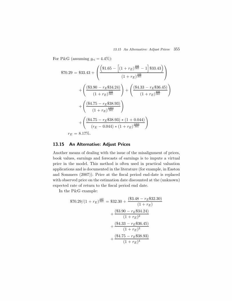
13.15 An Alternative: Adjust Prices 355

For P&G (assuming gri = 4.4%):

$70.29 = $33.43 +

($1.65 −

[(1 + rE)

168365 − 1

]$33.43

)(1 + rE)

168365

+

(($3.90 − rE$34.24)

(1 + rE)533365

)+

(($4.33 − rE$36.45)

(1 + rE)898365

)

+

(($4.75 − rE$38.93)

(1 + rE)1263365

)

+

(($4.75 − rE$38.93) ∗ (1 + 0.044)

(rE − 0.044) ∗ (1 + rE)1263365

)rE = 8.17%.

13.15 An Alternative: Adjust Prices

Another means of dealing with the issue of the misalignment of prices,book values, earnings and forecasts of earnings is to impute a virtualprice in the model. This method is often used in practical valuationapplications and is documented in the literature (for example, in Eastonand Sommers (2007)). Price at the fiscal period end-date is replacedwith observed price on the estimation date discounted at the (unknown)expected rate of return to the fiscal period end date.

In the P&G example:

$70.29/(1 + rE)197365 = $32.30 +

($3.48 − rE$32.30)(1 + rE)

+($3.90 − rE$34.24)

(1 + rE)2

+($4.33 − rE$36.45)

(1 + rE)3

+($4.75 − rE$38.93)

(1 + rE)4

356 Data Issues

+($4.75 − rE$38.93)

(rE − 4.4%) ∗ (1 + rE)4

rE = 8.2%

13.16 Summary

This section describes methods of dealing with data issues and ways ofestimating the cost of capital at any point in time. These issues willarise when using most sources of analysts’ earnings forecasts.

14

Some Thoughts on Future Directions

The literature on reverse-engineering accounting-based valuation mod-els has come a long way in a very short time, but we have a long wayto go. Estimates of firm-specific implied rates of return appear to bequite poor. The challenge is to improve the estimates. The question isHow?

14.1 Other Sources of Earnings Forecasts: The Data

In view of the fact that most studies have been based on I/B/E/Sforecasts, it is tempting to look to other sources, such as ValueLine orZack’s, taking the view that there is, as yet, no evidence that estimatesbased on these forecasts suffer the same short-comings as estimatesbased on I/B/E/S. This argument has been made in several studies butit is without foundation; it is likely that when subjected to rigoroustesting via methods such as Easton and Monahan (2005), estimatesbased on these data sources will also be found wanting.

Another approach has been to avoid use of earnings forecasts, andto, instead, rely on analysts’ forecasts of dividends and prices as in Bravet al. (2005). It would be surprising if these methods out-performed

357

358 Some Thoughts on Future Directions

the accounting-based estimates when subjected to rigorous analysis;nevertheless, the proof will be in the pudding.

14.2 Mitigating Errors and Bias

The vast literature on analysts’ forecasts provides a wealth of opportu-nities for mitigating/reducing the effects of errors in analysts’ forecasts.Much of this literature has focused on obtaining better estimates of themarket earnings expectations but the use of the better estimates hasbeen limited (for example, to obtain a better measure of the surprise inthe announcement of earnings). Reverse-engineering accounting-basedvaluation models provides a new, and important, context.

14.3 Refocus on Operations

I began this survey with a focus on the operations of the firm and Ishowed how: (1) the residual operating income model may be used tovalue the firm; and (2) we can reverse-engineer the residual operatingincome model to obtain estimates of the implied cost of capital for thefirm (otherwise known as the cost of capital for operations).

All of the methods of estimating the cost of equity capital at theportfolio level could be applied to estimating the cost of capital foroperations. We would need estimates of net operating profit after tax(NOPAT) and net operating asset (NOA). Nissim and Penman (2001)provides a template for calculating these items from Compustat data.Backing forecasts of NOPAT and NOA out of analysts’ forecasts willpose challenges, but these challenges are becoming less and less daunt-ing as analysts’ provide forecasts of more and more data other thanearnings.

References

Abarbanell, J. (1991), ‘Do analysts’ earnings incorporate informationin prior stock price changes?’. Journal of Accounting and Economics14, 147–166.

Ali, A., A. Klein, and J. Rosenfeld (1992), ‘Analysts’ use of informationabout permanent and transitory earnings components in forecastingannual EPS’. The Accounting Review 67(January), 183–199.

Barth, M. (1991), ‘Relative measurement errors among alternative pen-sion asset and liability measures’. The Accounting Review 66(July),433–463.

Berger, P., H. Chen, and F. Li (2006), ‘Firm specific information andcost of equity’. Working Paper, University of Chicago.

Berk, J., R. Green, and V. Naik (1999), ‘Optimal investment, growthoptions, and security returns’. Journal of Finance 54(October),1553–1607.

Botosan, C. (1997), ‘Disclosure level and the cost of equity capital’.The Accounting Review 72, 323–349.

Botosan, C. and M. Plumlee (2005), ‘Assessing alternative prox-ies for the expected risk premium’. The Accounting Review 80,21–54.

359

360 References

Botosan, C., M. Plumlee, and Y. Xie (2004), ‘The role of informa-tion precision in determining the cost of equity capital’. Review ofAccounting Studies 9, 233–259.

Bradshaw, M. (2004), ‘How do analysts use their earnings forecastsin generating stock recommendations?’. The Accounting Review 79,25–50.

Brav, A., R. Lehavy, and R. Michaely (2005), ‘Using expectations totest asset pricing models’. Financial Management 34, 31–64.

Brown, L. (1993), ‘Earnings forecasting research: It’s implications forcapital markets research’. International Journal of Forecasting 9,295–320.

Brown, L. (1997), ‘Earnings surprise research: Synthesis and perspec-tives’. Financial Analysts Journal 53, 13–19.

Brown, L. (2001), ‘A temporal analysis of earnings surprises: Profitsversus losses’. Journal of Accounting Research 39, 221–242.

Brown, L. (2003), ‘Small negative surprises: Frequency and conse-quences’. International Journal of Forecasting 19(January–March),149–159.

Brown, L., R. Hagerman, P. Griffin, and M. Zmijewski (1987), ‘Anevaluation of alternative proxies for the market’s assessment of unex-pected earnings’. Journal of Accounting and Economics 9, 159–193.

Brown, L. and M. Rozeff (1978), ‘The superiority of analyst forecastsas measures of expectations: Evidence from earnings’. Journal ofFinance 33, 1–16.

Capstaff, J., K. Paudyal, and W. Rees (1998), ‘Analysts’ forecasts ofGerman firms’ earnings: A comparative analysis’. Journal of Inter-national Financial Management and Accounting 9, 83–116.

Claus, J. and J. Thomas (2001), ‘Equity risk premium as low as threepercent? Evidence from analysts’ earnings forecasts for domestic andinternational stocks’. Journal of Finance 56, 1629–1666.

Cochrane, J. (2001), Asset pricing. Princeton, NJ: Princeton UniversityPress.

Collins, W. and W. Hopwood (1980), ‘A multivariate analysis of annualearnings forecasts generated from quarterly forecasts of financialanalysts and univariate time series models’. Journal of AccountingResearch 18, 390–406.

References 361

Conroy, R. and R. Harris (1987), ‘Consensus forecasts of corporateearnings: Analysts’ forecasts and time series methods’. ManagementScience 33(June), 725–739.

Das, S., B. Levine, and K. Sivaramakrishnan (1998), ‘Earnings pre-dictability and bias in analysts’ earnings forecasts’. The AccountingReview 73, 277–294.

Das, S. and S. Saudagaran (1998), ‘Accuracy, bias, and dispersion inanalysts’ earnings forecasts: The case of cross-listed foreign firms’.Journal of International Financial Management and Accounting 9,16–33.

Daske, H. (2006), ‘Economic benefits of adopting IFRS or US-GAAP —Have the expected costs of equity capital really decreased?’. Journalof Business, Finance, and Accounting 33, 329–373.

Daske, H., G. Gebhardt, and S. Klein (2006), ‘Estimating the expectedcost of equity capital using analysts’ consensus forecasts’. Schmalen-bach Business Review 58(January), 2–36.

Dhaliwal, D., L. Krull, O. Li, and W. Moser (2005), ‘Dividend taxes andimplied cost of capital’. Journal of Accounting Research 43, 675–715.

Dugar, A. and S. Nathan (1995), ‘The effect of banking relations onfinancial analysts’ earnings investment recommendations’. Contem-porary Accounting Research 12, 131–160.

Easton, P. (2001), ‘Discussion of: “When capital follows profitability:Non-linear residual income dynamics”’. Review of Accounting Studies6(June–September), 267–274.

Easton, P. (2004), ‘PE ratios, PEG ratios, and estimating the impliedexpected rate of return on equity capital’. The Accounting Review79, 73–96.

Easton, P. (2006), ‘Use of forecasts of earnings to estimate and comparecost of capital across regimes’. Journal of Business, Finance, andAccounting 33, 374–394.

Easton, P., T. Harris, and J. Ohlson (1992), ‘Aggregate earnings canexplain most of security returns: The case of long event windows’.Journal of Accounting and Economics 15(2/3), 119–142.

Easton, P. and S. Monahan (2005), ‘An evaluation of accounting-basedmeasures of expected returns’. The Accounting Review 80, 501–538.

362 References

Easton, P. and G. Sommers (2007), ‘Effects of analysts’ optimism onestimates of the expected rate of return implied by earnings fore-casts’. Journal of Accounting Research 45(December), 983–1015.

Easton, P., G. Taylor, P. Shroff, and T. Sougiannis (2002), ‘Using fore-casts of earnings to simultaneously estimate growth and the rateof return on equity investment’. Journal of Accounting Research40(June), 657–676.

Easton, P., J. Wild, R. Halsey, and M. McAnally (2008), FinancialAccounting for MBAs. Chicago, IL: Cambridge Business Publishers.

Elton, E. (1999), ‘Expected return, realized return, and asset pricingtests’. Journal of Finance 54(August), 1199–1220.

Fama, E. and K. French (1992), ‘The cross-section of expected returns’.Journal of Finance 47(June), 427–465.

Fama, E. and K. French (1997), ‘Industry costs of equity’. Journal ofFinancial Economics 43, 154–194.

Fama, E. and K. French (2002), ‘The equity premium’. Journal ofFinance 58(April), 609–646.

Feltham, G. and J. Ohlson (1996), ‘Uncertainty resolution and the the-ory of depreciation measurement’. Journal of Accounting Research34(Autumn), 209–235.

Francis, J., I. Khurana, and R. Periera (2005), ‘Disclosure incentivesand effects on cost of capital around the world’. The AccountingReview 80, 1125–1163.

Francis, J., R. LaFond, P. Olsson, and K. Schipper (2004), ‘Costs ofcapital and earnings attributes’. The Accounting Review 79, 967–1011.

Frankel, R. and C. Lee (1998), ‘Accounting valuation, market expecta-tions, and cross-sectional stock returns’. Journal of Accounting andEconomics 35, 283–319.

Fried, D. and D. Givoly (1982), ‘Financial analysts’ forecasts ofearnings: A better surrogate for market expectations’. Journal ofAccounting and Economics 4(October), 85–108.

Garber, S. and S. Klepper (1980), ‘Administrative pricing or competi-tion coupled with errors of measurement?’. International EconomicReview 21(June), 413–435.

References 363

Gebhardt, W., C. Lee, and B. Swaminathan (2001), ‘Towards an ex-ante cost of capital’. Journal of Accounting Research 39, 135–176.

Givoly, D. and J. Lakonishok (1984), ‘Aggregate earnings expectationand stock market behavior’. Journal of Accounting, Auditing, andFinance 2(Spring), 117–137.

Gode, D. and P. Mohanram (2003), ‘What affects the implied cost ofequity capital?’. Review of Accounting Studies 8, 399–431.

Guay, W., S. Kothari, and S. Shu (2005), ‘Properties of implied costof capital using analysts’ forecasts’. Working Paper, University ofPennsylvania, Pennsylvania, Wharton School.

Hail, L. and C. Leuz (2006), ‘International differences in the cost ofequity capital: Do legal institutions and securities regulation mat-ter?’. Journal of Accounting Research 44, 485–532.

Hribar, P. and N. Jenkins (2004), ‘The effect of accounting restatementson earnings revisions and the estimated cost of capital’. Review ofAccounting Studies 9, 337–356.

Huang, R., R. Natarajan, and S. Radhakrishnan (2005), ‘Estimatingfirm-specific long-term growth rate and cost of capital’. WorkingPaper. University of Texas at Dallas.

La Porta, R. (1996), ‘Expectations and the cross-section of stockreturns’. Journal of Finance 51, 1715–1742.

Lynch, P. (2000), One Up on Wall Street. New York, NY: Simon andSchuster, p. 199.

Lys, T. and S. Sohn (1990), ‘The association between revisions of finan-cial analysts’ earnings forecasts and security-price changes’. Journalof Accounting and Economics 13(December), 341–364.

Makridakis, S. and R. Winkler (1983), ‘Averages of forecasts: Someempirical results’. Management Science 29(September), 987–997.

Mendenhall, R. (1991), ‘Evidence on the possible underweighting ofearnings information’. Journal of Accounting Research 29, 170–179.

Modiglaini, F. and M. Miller (1958), ‘The cost of capital, corporationfinance, and the theory of investment’. American Economic Review48(June), 261–297.

Nissim, D. and S. Penman (2001), ‘Ratio analysis and equity valuation:From research to practice’. Review of Accounting Studies 6, 109–154.

364 References

O’Brien, P. (1988), ‘Analysts’ forecasts as earnings recommendations’.Journal of Accounting and Economics 10, 53–83.

Ogneva, M., K. R. Subramanyam, and K. Raghunandan (2007), ‘Inter-nal control weakness and cost of equity: Evidence from SOX section404 disclosures’. The Accounting Review 82(October), 1255–1298.

O’Hanlon, J. and A. Steele (2000), ‘Estimating the equity risk premiumusing accounting fundamentals’. Journal of Business Finance andAccounting 27, 1051–1084.

Ohlson, J. (1995), ‘Earnings, book values, and dividends in equity val-uation’. Contemporary Accounting Research 11(Spring), 661–688.

Ohlson, J. and Z. Gao (2006), ‘Earnings, earnings growth and value’.Foundations and Trends in Accounting.

Ohlson, J. and B. Juettner-Nauroth (2005), ‘Expected EPS and EPSgrowth as determinants of value’. Review of Accounting Studies10(June–September), 349–365.

Penman, S. (2007), Financial Statement Analysis and Valuation.McGraw-Hill.

Peters, D. (1993a), ‘Are earnings surprises predictable?’. Journal ofInvesting 2(Summer), 47–51.

Peters, D. (1993b), ‘The influence of size on earnings surprise pre-dictability’. Journal of Investing 2(Winter), 54–59.

Richardson, S., S. Teoh, and P. Wysocki (2004), ‘The walk-down tobeatable analyst forecasts: The role of equity issuances and insidertrading incentives’. Contemporary Accounting Research 21, 885–924.

Stober, T. (1992), ‘Summary financial statement measures and ana-lysts’ forecasts of earnings’. Journal of Accounting and Economics15(June–September), 347–373.

Vuolteenaho, T. (2002), ‘What drives firm-level stock returns?’. Journalof Finance 57(October), 233–264.

White, H. (1980), ‘A heteroscedasticity-consistent covariance estimatorand a direct test for heteroscedasticity’. Econometrica 48, 817–838.

Williams, M. (2004), ‘Discussion of “The role of information precisionin determining the cost of equity capital”’. Review of AccountingStudies 9, 261–264.

Zhang, X. (2000), ‘Conservative accounting and equity valuation’. Jour-nal of Accounting and Economics 29(February), 125–149.

estimating the cost of capital implied by market prices and accounting...

Documents