Economic Commission for Europe Conference of European Statisticians

Joint Eurostat/UNECE Work Session on Demographic Projections Geneva, 18-20 April 2016 Item 3 of the provisional agenda Sub-national projections Estimating sub-national behaviour in the Danish microsimulation model SMILE

by Marianne Frank Hansen, Tobias Ejnar Markeprand & Peter Stephensen1

Summary

The SMILE model is a Danish dynamic microsimulation model, which forecasts demography, household formation, housing demand, socioeconomic and educational attainment, income, taxation, and labour market pensions until the year of 2040. In the most recent version of the model, SMILE 3.0, selected behavioural patterns are allowed to vary across the 98 municipalities of Denmark. Especially, this provides the model with a detailed description of sub-national moving behaviour, which is essential when seeking to identify geographic areas characterized by a future positive or negative population growth.

Modelling behavioural patterns by a large number of potentially high dimensional covariates allows for a rich description of individual behaviour, but simultaneously reduces the number of observations with identical characteristics. Hence, due to data sparsity the curse of dimensionality following from introducing detailed sub-national behaviour significantly challenges the estimation of municipality dependant transition probabilities. This paper suggests the use of a combination of Principal Component Analysis (PCA) and classification by Conditional Inference Trees (CTREEs) when estimating transition probabilities depending on a large number of high dimensional covariates, hence overcoming the curse of dimensionality. The method is described and results are given.

Keywords: sub-national population projections, household projections, microsimulation, conditional inference trees, principal component analysis.

1 DREAM (www.dreammodel.dk), Denmark. This paper is largely an extract of the paper “Residential Choice in the Danish Microsimulation Model SMILE” by Marianne Frank Hansen, Tobias Ejnar Markeprand, and Peter Stephensen (2015).

Working paper 6

Distr.: General 30 March 2016 English only

2

I. Introduction

1. The SMILE2 model is a Danish dynamic microsimulation model, which forecasts demography, household formation, housing demand, socioeconomic and educational attainment, income, taxation, and labour market pensions of the entire Danish population until the year of 2040. In the most recent version of the model, SMILE 3.0, behavioural patterns are allowed to vary across the 98 municipalities of Denmark. Specifically, this equips the model with a detailed description of sub-national moving behaviour, which is essential when seeking to identify geographic areas characterized by a future positive or negative population growth.

2. Modelling behaviour by a large number of high dimensional covariates seems attractive when attempting to illuminate social and regional differences. Unfortunately, this tends to reduce the number of observations with identical characteristics, thus inducing the curse of dimensionality.

3. To overcome this sparsity challenge, transition probabilities in SMILE are estimated using a data mining classification procedure. Data mining transition probabilities by using the conditional inference tree (CTREE) algorithm is found to be useful in order to quantify a discrete response variable conditional on multiple individual characteristics. Classifying observations by CTREEs tends to give rise to better covariate interactions than traditional parametric discrete choice models, i.e. logit and probit models, cf. Fernandez-Delgado, M., Cernadas, E. & Barro, S. (2014)3.

4. Estimating responses across multiple high dimensional characteristics can however lead to lacking convergence of the classification algorithm. Though facilitating an enriched characterization of individual behaviour, increasing the dimension of the geographical component of the model from describing behaviour across 11 regions to 98 municipalities turns out to constitute a significant challenge regarding convergence. The lack of convergence can be overcome by ordering the entries of certain feature variables, hereby restricting the classification options of the CTREE algorithm. Principal component analysis (PCA) is introduced as a tool for deciding on the ordering sequence of the entries of the geographic feature variables, hereby constituting an unsupervised learning pre-process enabling convergence of the classification algorithm.

5. Section II summarizes the CTREE classification algorithm supported by a few examples. The following subsection explains the difference between ordered and non-ordered variables as well as the restrictions hereby imposed on classification. Subsequently, principal component analysis is introduced and applied to rank the Danish municipalities, which constitute the entries of the geographic feature variables

2 Simulation Model of Individual Lifecycle Evaluation. 3 However, the opposite might be true if logit or probit models are applied to a tuned selection of covariates and covariate interactions.

3

entering as covariates in the classification algorithm. A conclusion is provided in section III.

II. Estimating transition probabilities

6. The rich register data from Statistics Denmark allows for the initial population in SMILE to be constituted of the entire Danish population of 2013 distributed on a vast range of demographic, educational, socioeconomic, and dwelling related characteristics. The population is divided into households in order to allow for events simultaneously affecting all individuals of a household. During each forecast year the households are exposed to a series of events allowing the household or its individual members to transfer from one state to another. The occurrence of an event is decided by Monte Carlo simulation and an estimated transition probability describing the likeliness of the event from a series of household or individual specific characteristics. Determining transition probabilities is therefore a vital part of most dynamic microsimulation models. In SMILE transition probabilities are used to determine events regarding demography, family formation, educational and socioeconomic attainment as well as events regarding residential choice, cf. Hansen, J. Z. & Stephensen, P. (2013) and Hansen M.F. & Markeprand T. (2015).

Conditional inference trees - CTREEs 7. As mentioned in the introduction describing behavioural patterns by a large number of

high dimensional covariates seems appealing when attempting to illuminate social and regional differences. The hereby induced curse of dimensionality challenges the possibility of estimating responses as raw probabilities. Further, in the case of policy changes the model is likely to produce future states with very few or without previous instances. A frequency based calculation of transition probabilities, will not allow for behaviour being estimated for unprecedented states.

8. In SMILE the sparsity challenge is met by estimating transition probabilities by a data mining approach. The conditional inference tree (CTREE) algorithm is used to classify observations with similar responses across a vast range of characteristics. Describing the response by multiple characteristics leads to the possible presence of correlation between the features. However, this is of less importance when applying classification by conditional inference trees. Considerations regarding the use of feature selection therefore become redundant. Apart from accommodating the curse of dimensionality, classification also facilitates the estimation of behaviour related to unprecedented states.

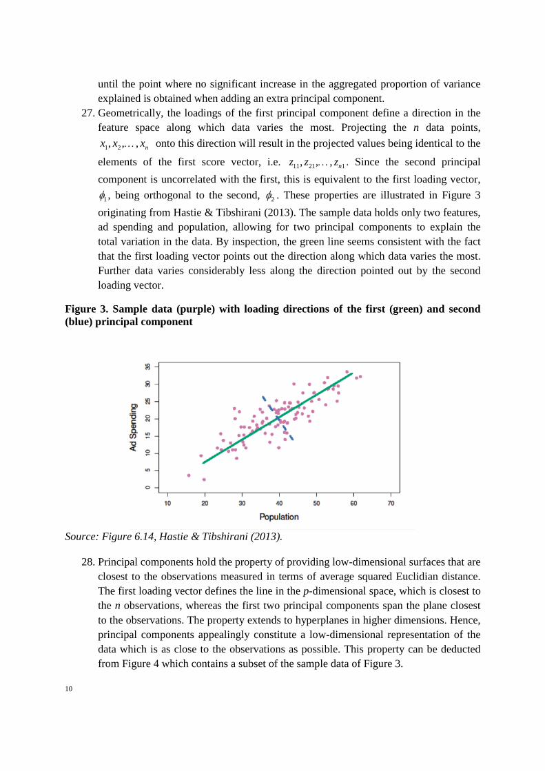
9. Using recursive binary partitioning, classification by conditional inference trees (CTREEs) constitutes an algorithm for grouping individuals’ responses according to a range of conditioning covariates. CTREE is one of the most recent algorithms serving this purpose, cf. Hothorn, Hornik & Zeileis (2006). Recursively splitting the population by characteristics results in smaller groups consisting of individuals with

4

identical behaviour, i.e. identical responses regarding a specific event. Classification is induced by recognized statistical procedures evaluating heterogeneity and the number of observations within the group exposed to a potential split. If a split is statistically validated, binary partitioning results in two new tree nodes, each of which can potentially split further after the next evaluation. The recursion stops when indicated by the statistical test procedures. Nodes caused by the final split are called terminal nodes. The final tree is characterized by a minimum of variation in the response between observations within a terminal node and maximum variation across terminal nodes. For each terminal node a transition probability is calculated and used to describe the response of individuals with the same covariate structure as characterizing the given terminal node.

10. For example, if a terminal node consists of single men aged 60 or above with a basic education and couples aged between 40 and 50, this indicates that the classification algorithm does not detect a significant difference in behaviour between the two household types. A common transition probability is calculated from all the observations classified within the group hereby creating a probability estimate, which is identical across several feature variables. Hence, by applying a classification algorithm to the data, the sparsity problem can be overcome.

11. The CTREE-algorithm can be summarized in three steps (for details see Hothorn, Hornik, Strobl & Zeileis 2013):

1) Test the global null hypothesis of independence between any of the explanatory

variables and the response. a. Stop if this hypothesis cannot be rejected (p>0.05). b. Otherwise select the input variable with strongest association to the response. This

association is measured by a p-value corresponding to a test for the partial null hypothesis of a single input variable and the response. For SMILE we choose to use the default implementation with cquad-type test statistics and Bonferroni-adjusted p-values to avoid overfitting.

2) Implement a binary split in the selected input variable. To find the optimal binary

split in the selected input variable the algorithm uses a permutation test. The default stopping criterion ensures that groups containing less than 20 observations will not be split and that the groups resulting from a split will contain at least 7 observations.

3) Recursively repeat steps 1) and 2) until a stopping criterion is reached.

5

12. Since the algorithm is capable of handling a large number of feature variables the need for domain specific knowledge otherwise required when deciding on which explanatory variables to include or group is reduced. Unlike similar recursive fitting algorithms CTREEs are not biased towards selecting input variables with many missing values or many possible splits. The CTREE-framework is applicable to a wide range of regression problems where both response and covariates can be measured at arbitrary scales, including nominal, ordinal, discrete and continuous as well as censored and multivariate variables.

An example

13. Figure 1 contains an example of the structure of a very simple CTREE. The CTREE is based on dummy data but provides an illustration of how recursively splitting the data set by the elements of the explanatory variables leads to the estimation of transition probabilities across multiple features.

Figure 1. The structure of a CTREE.

Note: The transition probability for a couple with an average age of 24 is 17 % while the transition probability for a single 20-year old male is 21 %. A family with an average age of 42 with a compulsory education experiences the occurrence of the event with a probability of 11 %.

14. The first split concerns the average age of the adults in the family, while the second split depends on the outcome of the first split. If the average age is above 25 the next split depends on the level of educational attainment while in the opposite case the second split is conditional on whether the household consists of one or two adults. In order to determine the estimated transition probability the tree structure must be

6

followed downwards until a terminal node is reached. Splits can be performed on both continuous and categorical data. By specifying explanatory variables as continuous, the numerical order of the input variable will be respected, hereby restricting the structure of the splits. Age is a continuous variable. This means that the algorithm can group families with an average age above 25 but cannot perform a split that places 16- and 18-year olds together while at the same time placing 15- and 17-year olds in a group of their own. In this case age is said to be an ordered variable. In the next section a discussion of the difference between ordered and non-ordered variables is provided. This issue is important since the nature of the explanatory variables matters profoundly on the convergence ability of the CTREE algorithm, i.e. the ability of the algorithm reaching a stopping criterion. In the example above, each terminal node contains a transition probability representing the likeliness of a decision with a binary outcome occurring (event vs. non-event). In SMILE CTREEs are used to estimate responses with binary outcomes as well as responses with multiple outcomes (multinomial classification).

15. Providing an additional example4, the result of applying the CTREE algorithm to data describing the decision of moving is illustrated in Figure 2, where the age dependent moving probabilities calculated by frequencies are compared to probabilities resulting from applying the CTREE algorithm. Probabilities estimated by the frequency approach fluctuate around the behaviour resulting from classification. The flat sections of the moving probabilities estimated by the CTREE indicate that the algorithm groups subjects within the given age intervals. For example, individuals aged between 20 and 27 are found to exhibit identical moving behaviour. The same is the case for individuals aged 85 or above.

Figure 2. Estimated moving probabilities of single males.

Source: Calculations performed on register data from Statistics Denmark. 4 More examples are provided in Rasmussen, N. E., M. F. Hansen & P. Stephensen (2013). For an introduction to big data analysis and CTREEs, Varian (2014) is recommendable.

0

0.1

0.2

0.3

0.4

0.5

0 5 10 15 20 25 30 35 40 45 50 55 60 65 70 75 80 85 90 95100

Pro

babi

lity

CTREE No classification modelAge

7

Ordered and non-ordered variables 16. As mentioned previously the CTREE algorithm might experience difficulties

converging. Hence the test statistic will continuingly establish a significant relationship between the response and an explanatory variable, indicating a tendency of splitting the data into groups consisting of the smallest possible number of observations defined by the stopping criterion. In the absence of a stopping criterion, this could consequently lead to a classification result similar to what would be the outcome of a simple frequency calculation, hereby leaving the challenge of data sparsity unresolved.

17. The nature of the feature variables has a considerable influence on the chance of convergence. The feature variables will typically appear as either ordered or non-ordered. An ordered variable is characterized by its set elements appearing in a logical order whereas there is no predefined sequence for the set elements of a non-ordered variable. Categorical variables are traditionally non-ordered whereas the elements of numerical variables tend to have a logical order attached to them. For example, it seems reasonable that a variable describing age consists of ordered elements whereas no objective ordering of variable elements defining labour market participation comes into mind.

18. The ordered or non-ordered nature of a variable restricts the classification options of the CTREE algorithm. When an ordered variable is selected for splitting in step 1b, only observations with adjacent values of the given variable will be grouped in the particular split. I.e. when splitting on the ordered variable age, individuals under the age of 20 cannot be grouped with individuals aged 50 or above, hereby leaving individuals of the remaining ages in a group of their own. Rather the observations might be split into two groups consisting of people aged below or above 20 respectively. If the age variable for the group holding individuals aged above 20 subsequently is reselected for splitting, then at this stage the individuals can be grouped depending on whether the subject is aged above 50 or between 20 and 50. Since the observations are grouped by age in multiple splits, it is unlikely that the classification results in similar behaviour with respect to the response of individuals aged below 20 and above 50. In the case of the age variable being non-ordered there is no hindrance for a single split classifying observations in the aforementioned non-adjacent age intervals into the same group.

19. Allowing demography, moving propensities and residential choice to vary across municipalities induces lacking convergence of the CTREE algorithm when the municipality information is included as a non-ordered feature variable. Restricting the classification procedure by ordering the set elements of the municipality variable can however lead to convergence of the algorithm and hence result in estimation of municipality dependent responses. As stated above, the choice of ranking is essential, thus imposing a challenge when no immediate sequence appears logical. An ordering sequence could be chosen by ranking the municipalities according to a specific

8

feature, i.e. labour market participation rate, educational attainment, tax/service ratio, median, or average income, hereby insuring that municipalities with similar features are more likely to be grouped by the CTREE algorithm. However, classification might depend profoundly on the choice of ranking measure used. In the following section principal component analysis is introduced as providing a tool for choosing the ordering sequence of the municipality variable, thus allowing the ranking to spring from multiple features.

Ordering variables by principal component analysis 20. While classification is an example of a supervised learning method, principal

component analysis is an example of an unsupervised learning technique. In both settings we have access to a number of feature variables describing a set of observations, but the response is only known in the case of supervised learning. Hence, predicting the response is not the objective when applying an unsupervised learning method. Rather such methods are applied to discover certain patterns in the data, such as subgroups across the features or within the observations. Clustering is another example of an unsupervised learning algorithm5. While a supervised learning method allows for testing of estimation accuracy, this is not the case in an unsupervised learning setting given the nature of no response. However, applying the result of an unsupervised learning method as a pre-process to supervised learning, will allow for an implicit testing of the unsupervised outcome within the supervised framework.

21. When faced with a number of observations characterized by a large set of potentially correlated variables, principal component analysis can be used to summarize this set by a smaller number of representative independent variables that explain most of the variability in the original set. Principal component analysis is not a feature selection tool but can be used to deduct a low-dimensional representation of the data set, which explains a significant part of the total variance. Finding a low-dimensional representation can also be useful to visualize a largely dimensioned data set. In order to understand how PCA can help us finding a ranking order of the elements of the municipality variable used in classification, the method is introduced in the following section.

Principal component analysis 22. Assume that we have a data set with n observations described by p features, i.e. we

have p variables 1 2, , , pX X X each of dimension n. Each observation is described in

p dimensions which are unlikely to be of equal interest. Some variables might be of

5 Clustering methods have been applied to the data attempting to determine an initial disaggregation of the data set that would allow for convergence of the CTREE algorithm without ordering the set elements of the municipality variable. The suggested grouping of the observations did however not allow for a successful application of the CTREE method. Further, experiments with a less restrictive stopping criterion of the classification algorithm have been performed.

9

lesser importance if the observations are correlated across several features or simply do not vary along a given dimension. PCA seeks to identify a low-dimensional space that contains a significant part to total data variability along each of its dimensions. Each of these dimensions can be represented by a principal component which is found to be a restricted linear combination of the p features in the data set.

23. The first principal component is the linear combination of the p features that has the largest variance, subject to the coefficients being normalized.

1 1 2 2k k k pk pZ X X Xφ φ φ= + + + 24. That is, we solve the following problem

2 21 1

1 1

1max s.t. 1pn

i ji j

zn

φ= =

=

∑ ∑

where 1 11 1 21 2 1i i i p ipz x x xφ φ φ= + + + and we have assumed, that each of the p features have been centered to have zero mean. The elements of the coefficient vector

( )1 11 21 1, , , pφ φ φ φ= are referred to as loadings of the first principal component

whereas the n entries of the first principal component vector 11 21 1, , , nz z z… are referred to as scores. The loadings have been normalized to guarantee a unique solution to the maximization problem, since otherwise variation could be chosen arbitrarily large simply by increasing the loadings. The optimization problem can be solved by eigen decomposition which is outside the scope of this paper.

25. After having determined the first principal component, 1Z , the second principal

component, 2Z , can be found. The latter is defined as the linear combination of

1 2, , , pX X X that has the largest variance out of all linear combinations that are

uncorrelated with 1Z . Under the restriction of independency between principal components, we solve the following problem

2 22 2

1 1

1max s.t. 1pn

i ji j

zn

φ= =

=

∑ ∑

26. By following the above procedure, and hence conditioning on the independence

between principal components, we are able to subsequently deduct as many as k principal components, where min( 1, )k n p= − . Calculating the proportion of the total variance in the data explained by each component can be used to decide on the number of principal components constituting a reasonable low-dimensional representation of the data. The basic rule is to include principal components in the data representation

10

until the point where no significant increase in the aggregated proportion of variance explained is obtained when adding an extra principal component.

27. Geometrically, the loadings of the first principal component define a direction in the feature space along which data varies the most. Projecting the n data points,

1 2, , , nx x x… onto this direction will result in the projected values being identical to the

elements of the first score vector, i.e. 11 21 1, , , nz z z… . Since the second principal component is uncorrelated with the first, this is equivalent to the first loading vector,

1φ , being orthogonal to the second, 2φ . These properties are illustrated in Figure 3 originating from Hastie & Tibshirani (2013). The sample data holds only two features, ad spending and population, allowing for two principal components to explain the total variation in the data. By inspection, the green line seems consistent with the fact that the first loading vector points out the direction along which data varies the most. Further data varies considerably less along the direction pointed out by the second loading vector.

Figure 3. Sample data (purple) with loading directions of the first (green) and second (blue) principal component

Source: Figure 6.14, Hastie & Tibshirani (2013).

28. Principal components hold the property of providing low-dimensional surfaces that are closest to the observations measured in terms of average squared Euclidian distance. The first loading vector defines the line in the p-dimensional space, which is closest to the n observations, whereas the first two principal components span the plane closest to the observations. The property extends to hyperplanes in higher dimensions. Hence, principal components appealingly constitute a low-dimensional representation of the data which is as close to the observations as possible. This property can be deducted from Figure 4 which contains a subset of the sample data of Figure 3.

11

Figure 4. Sample data with loading direction and score values of the first principal component

Note: The blue dot indicates average population and ad spending. Source: Figure 6.15, Hastie & Tibshirani (2013).

29. The loading vector of the first principal component is the line closest to the observations measured by the sum of the squared distances identified by the black dashed lines. The dashed black lines projects the observations onto the loading vector, hence allowing the projected values to be identified as the scores of the first principal component. The score values of the first and second principal component are depicted in the right-hand side of Figure 4.

30. Since each principal component spans the variability of the data in a given dimension, observations with neighbouring score-values of a specific principal component are considered to be more similar than observations represented by more widely differing scores-values. E.g. observations with score-values in each end of the green line in Figure 4 are mutually more different than observations lying in the middle of the line. This suggests that we can use the order of score-values of one or more principal components to rank the Danish municipalities when these are described from a vast range of features. The subsequent paragraph will clarify how this is done.

Ranking municipalities by principal component score-values

31. Data describing 60 fundamental demographic, socioeconomic, and economic features of each of the 98 Danish municipalities are retrieved from the Municipality Fundamentals Database of The Ministry of Social Affairs and the Interior6. The selected features are averaged over the years ranging from 2007 to 2014, hereby

6 In Danish: Social- og Indenrigsministeriets database over kommunale nøgletal.

12

reducing the impact of business cycle effects and local policy on the principal components7.

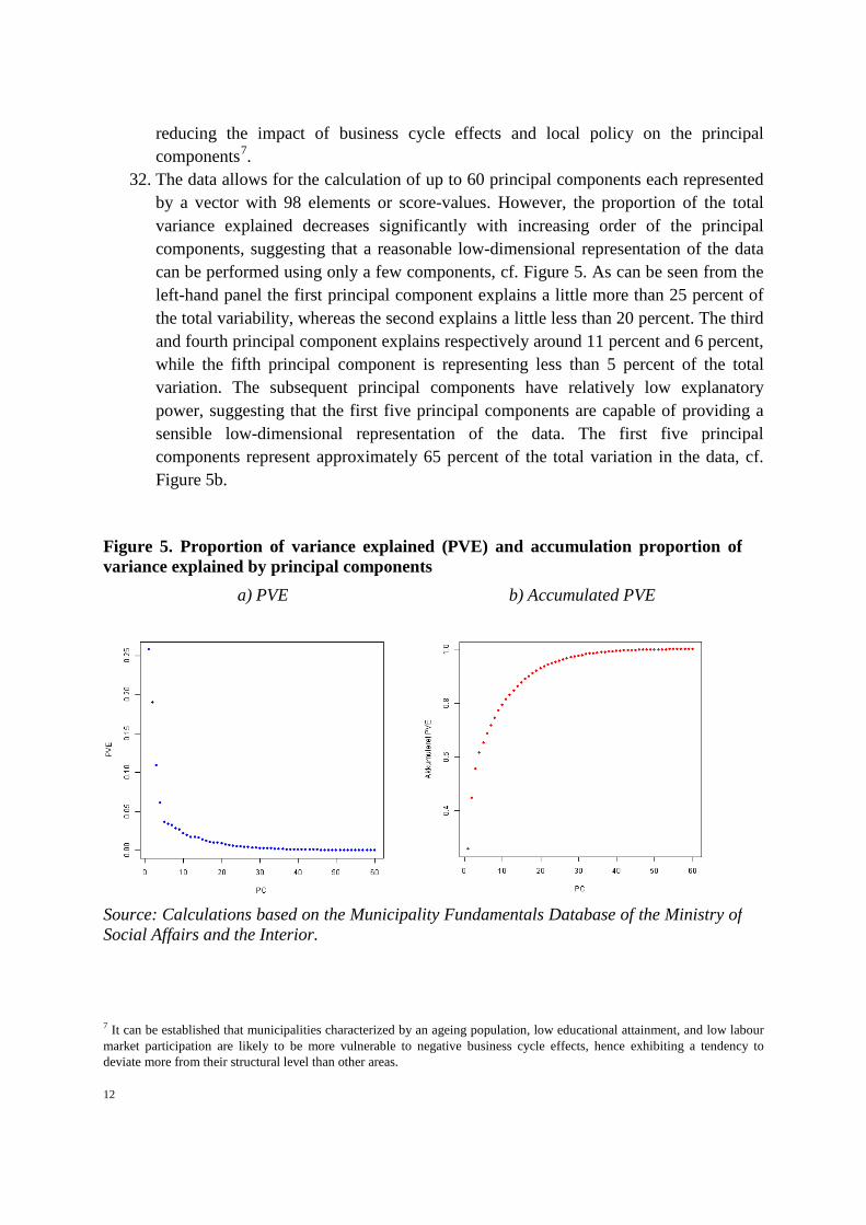
32. The data allows for the calculation of up to 60 principal components each represented by a vector with 98 elements or score-values. However, the proportion of the total variance explained decreases significantly with increasing order of the principal components, suggesting that a reasonable low-dimensional representation of the data can be performed using only a few components, cf. Figure 5. As can be seen from the left-hand panel the first principal component explains a little more than 25 percent of the total variability, whereas the second explains a little less than 20 percent. The third and fourth principal component explains respectively around 11 percent and 6 percent, while the fifth principal component is representing less than 5 percent of the total variation. The subsequent principal components have relatively low explanatory power, suggesting that the first five principal components are capable of providing a sensible low-dimensional representation of the data. The first five principal components represent approximately 65 percent of the total variation in the data, cf. Figure 5b.

Figure 5. Proportion of variance explained (PVE) and accumulation proportion of variance explained by principal components

a) PVE b) Accumulated PVE

Source: Calculations based on the Municipality Fundamentals Database of the Ministry of Social Affairs and the Interior.

7 It can be established that municipalities characterized by an ageing population, low educational attainment, and low labour market participation are likely to be more vulnerable to negative business cycle effects, hence exhibiting a tendency to deviate more from their structural level than other areas.

13

33. Figure 6 and Figure 7 contain a geographical representation of the score-values of the first and second principal component. From Figure 6 it can be seen that municipalities that are either coinciding with the major cities or situated in the close vicinity of these, are likely to have neighbouring score-values of the first principal component. These municipalities are characterized by a greenish colour. Especially, it is noticeable that the municipalities in a vast range of Copenhagen are of similar colour, which is however gradually fading with increasing distance from the capital. On Funen and in Jutland the contrast between the municipalities hosting the major cities and their immediate neighbours is somewhat larger. In Figure 7 the major cities are again identified by having similar score-values of the second principal component. However, opposite to the scores of the first principal component, this similarity is now shared with the islands south of Zeeland, Bornholm as well as the sparsely populated small islands. Further, it should be noticed that the score-values changes immediately and to a remarkable extent when moving to the suburbs of the major cities. E.g. the suburbs of Copenhagen, Aarhus, and Aalborg exhibit strong positive score-values indicated by the vibrant blue colour, whereas negative values can be observed for the neighbouring major city municipalities.

Figure 6. Score-values of the first principal component by municipality

Source: Calculations based on the Municipality Fundamentals Database of the Ministry of Social Affairs and the Interior.

14

Figure 7. Score-values of the second principal component by municipality

Source: Calculations based on the Municipality Fundamentals Database of the Ministry of Social Affairs and the Interior.

34. The correlation between the feature variables and each of the principal components has been calculated in order to aid the interpretation of the variability represented by each principal component. Since the proportion of variance explained decreases with increasing order of the principal components, so does the correlation with the feature variables. The interpretability of higher order principal components can therefore become somewhat unclear. Therefore, only the first two principal components are subject to analysis in this section.

35. The first principal component exhibits a strong negative correlation with variables expressing the share of population living in urban housing, the share of the population commuting, per capita revenue from real estate and income taxes, land value per capita, the share of social housing, the share of citizens having a high level of educational attainment, population density, and share of Western immigrants. High values of these variables are traditionally associated with a high degree of urbanisation, hence the first principal component can to a wide extent be thought of as representing the level of urbanisation. Due to the aforementioned negative correlation

15

between these features and the scores values of the first principal component, small score-values indicate a high degree of urbanisation. The score-values are positively correlated with variables indicating geographical area size, home ownership housing as a share of total housing, the share of the population with low educational attainment, and the share of the population aged above 65. Municipalities outside the urban hubs are characterized by having high values of these features and are then associated with high score-values of the first principal component. In general the first principal component exhibits the strongest absolute correlation with features that are to be considered somewhat rigid, hence the features can be characterized as structural.

36. The second principal component is negatively correlated with variables indicating the expenditure needs of the municipalities. Municipalities with high levels of expenditure per capita, high expenditures per student in basic education, a large share of the population having only obtained basic educational skills, and a large share of total housing being social are linked to low score-values of the second principal component. The same is the case when the number of cash benefit recipients, early retirement recipients and unemployed is high. Oppositely, high score-values are associated with high levels of income tax revenue per capita and high land value per capita. Further, there is a strong positive correlation between the share of total housing being owner occupied, the share of the population with higher educational attainment, and the scores of the second principal component.

37. The second principal component can be interpreted as representing the budget balance of the municipalities8, and hence the average socioeconomic status of its citizens. As previously mentioned, the municipalities situated in the suburbs of the major cities are characterised by having higher score-values than the municipalities of these cities. This suggests than when controlling for the level of urbanisation, the labour market attainment and taxable income is somewhat higher in the suburban areas. This is emphasized by the fact that the municipalities of the major cities experience a high degree of ingoing commuting, which is mirroring the high tendency of outgoing commuting from the suburban areas.

38. Equivalently to Figure 4, Figure 8 depicts the relationship between the first and second principal component. Moving from the left to the right on the horizontal axis represents a shift from municipalities associated with a high degree of urbanisation to municipalities characterized by more rural structural features. The municipality of Copenhagen lies farthest to the left, whereas the small rural islands are almost consistently grouped to the right. On the contrary, the second principal component depicted on the vertical axis, places the capital on the same level as the aforementioned islands, hereby stating the mutual socioeconomic features of these areas. It should be noticed that the variability along the primary axis is somewhat

8 The principal component analysis is performed on the basis of variables, which have not been altered by municipal equalization. Therefore, the true budget balance can be represented by these variables.

16

similar to the variability along the secondary axis. This is consistent with the first and second principal component explaining an almost similar proportion of the total variance in the data, cf. Figure 5.

Figure 8. Relationship between the score-values of the first and second principal component, identified by municipalities

Source: Calculations based on the Municipality Fundamentals Database of the Ministry of Social Affairs and the Interior.

39. After having performed the principal component analysis, the municipalities are ranked according to the score-values of each of the principal components, which have been chosen to constitute the low-dimensional representation of the data set. The PVE provides some initial guidelines to this selection. Each ranking identifies an ordered variable with can be included as an explanatory variable in the CTREE. Due to the independence between principal components, the ranking of the municipalities is most likely to differ across principal components, hence allowing for less restrictive splits in the classification. E.g. the municipalities of Frederiksberg, Gentofte, and Copenhagen are ranked sequentially according to the first principal component, whereas they are far from immediate neighbours when judging from the ranking induced by the second principal component. This allows for a less restrictive classification and hence a more flexible estimation of behaviour with respect to the response being targeted by classification. Initially, it was mentioned that a single ranking measure is likely to be too restrictive. The final number of principal

17

components used in the CTREE is decided by testing model accuracy on a test data set when including one to five principal components in the classification procedure. Typically, this suggests the use of two or three principal components in the classification method.

III. Conclusion

40. Ranking covariate elements by the score values of a principal component is found to aid convergence of the CTREE classification algorithm, when classifying a response depending on high dimensional covariates. In SMILE this allows for estimation of municipality specific transition probabilities. Using the result of a principal component analysis further has the advantage of letting the ordering sequence of the municipality variable spring from multiple features. However, it should be mentioned that ranking municipalities according to a single measure highly correlated with, or in the binary case identical to, the response targeted in classification, is found to lead to a marginal improvement of estimation accuracy. Applying PCA, and hence sequencing the municipality elements from multiple features, is found to constitute a more general and universal applicable ranking measure since independent of the classification response.

41. It is vital to state, that classification results in behaviour being averaged across observations within a subgroup, hereby providing the group estimate. By definition this will clutter observation specific characteristics, but since grouping is decided by hypothesis testing, this should not lead to a significant information loss, but may induce a minor trend shift between observed and forecasted responses. To avoid extending business cycle effects observations are generally classified with respect to responses observed from 2000 to 2013. Hence, the forecast cannot be expected to constitute an extension of the response behaviour from the most recent two or three years.

18

References

Fernandez-Delgado, M., Cernadas, E. & Barro, S. (2014): Do we Need Hundreds of Classifiers to Solve Real World Classification Problems?, Journal of Machine Learning Research 15, 3133-3181.

Hansen, M. F & Markeprand T. (2015): Fremskrivning af familiekarakteristika og boligefterspørgslen i danske kommuner, DREAM Report, September 2015. The report can be downloaded from www.dreammodel.dk/SMILE. (Only Danish version available).

Hansen, M.F., Markeprand T. & Stephensen P. (2015): Residential choice in the Danish microsimulation SMILE, October 2015. The paper is available upon request.

Hansen, J. Z., Stephensen, P. & Kristensen, J. B. (2013): Household Formation and Housing Demand Forecasts, DREAM Report, December 2013. The report can be downloaded from www.dreammodel.dk/SMILE

Hansen, J. Z. & Stephensen, P. (2013): Modeling Household Formation and Housing Demand in Denmark using the Dynamic Microsimulation Model SMILE, DREAM Conference Paper, December 2013. The paper can be downloaded from www.dreammodel.dk/SMILE

Hastie, T., R. Tibshirani (with G. James & D. Witten) (2013): An Introduction to Statistical Learning, Springer.

Hothorn, T., K. Hornik & A. Zeileis (2006): Unbiased Recursive Partitioning: A Conditional Inference Framework, Journal of Computational and Graphical Statistics, Vol. 15, No. 3, page 651–74.

Hothorn, T., Hornik, K, Strobl, Carolin & Zeileis, A. ‘Party’ package for R: A Laboratory for Recursive Partytioning, October 2013, http://cran.r-project.org/web/packages/party/party.pdf

Rasmussen, N. E., M. F. Hansen & P. Stephensen (2013): Conditional inference trees in dynamic microsimulation - modelling transition probabilities in the SMILE model, DREAM Conference Paper, December 2013. The paper can be downloaded from www.dreammodel.dk/SMILE Stephensen, P. (2013): The Danish microsimulation model SMILE - An overview, DREAM Conference Paper, December 2013. The paper can be downloaded from www.dreammodel.dk/SMILE

Stephensen, P. (2015): The Event-Pump: An Agent-Based approach to Microsimulation, Fifth World Congress of the International Microsimulation Association (IMA).

Stephensen, P. & Markeprand, T. (2013): SBAM: An Algorithm for Pair Matching. The 4th General Conference of the International Microsimulation Association.

Varian, H. R. (2014): "Big Data: New Tricks for Econometrics." Journal of Economic Perspectives, 28(2): 3-28.