Estimating Soil Moisture and Electrical Conductivity Using Wi-Fi

Jian DingMicrosoft Research

Ranveer ChandraMicrosoft Research

Abstract

Soil Moisture and Soil Electrical Conductivity (EC) are im-portant parameters for data-driven farming. This knowledgecan help a farmer improve crop yield, reduce input costs, andadopt sustainable agriculture practices. However, the highcost of commercial soil moisture and EC sensors has lim-ited their adoption. In this paper, we present the design andimplementation of a system, called SMURF, that senses soilmoisture and soil EC using RF propagation in existing Wi-Fibands. It overcomes the key challenge of limited bandwidthavailability in the 2.4 GHz unlicensed spectrum using a novelmulti-antenna technique that maps the propagation time andamplitude of Wi-Fi to the different antennas as a function ofthe refractivity and permittivity of soil, and uses them to infersoil moisture and EC. Our experiments with software definedradios (USRP and WARP), and two commodity Wi-Fi cardsshow that SMURF can accurately estimate soil moisture andEC using Wi-Fi, thereby enabling a future in which a farmerwith a smartphone that has a Wi-Fi radio can sense soil in herfarm without investing 100s of dollars in soil sensing equip-ment.

1 Introduction

Several agricultural applications rely on soil moisture andsoil EC measurements. For example, precision irrigation,which refers to the variable application of water in differ-ent regions of the farm, depends on accurate soil moisturevalues at different depths. This helps reduce the amount ofwater use, and also reduces the leeching of ground water bythe contaminants used in fertilizers and other agricultural in-puts. Soil EC is another key indicator of soil health. It hasbeen shown to correlate very well with crop yield and plantnutrient availability, and farmers are recommended by theUSDA to measure soil EC to determine soil treatment plansand management zones for Precision Agriculture [1].

Several techniques have been invented over the last fewdecades to measure soil moisture and EC. These methods

include direct sensing techniques, that require soil to be ex-tracted and dried out, as well as indirect sensing methods thatmeasure surrogate properties of soil moisture and EC, suchas capacitance, electrical, and nuclear response. Researchershave also explored the use of radar based technologies tomeasure soil moisture and EC.

However, one of the key challenges in the adoption of soilmoisture and EC sensing technologies is the cost of existingsensor solutions. Although hobbyist soil moisture sensorsare available for less than 10 dollars, they are not reliableand degrade quickly, and are consequently not used by agri-cultural experts [2]. We are not aware of any low cost soilEC sensor. The lowest cost, commercial grade, soil mois-ture or soil EC sensing solutions still cost over a 100 dollars.They use ruggedized components that typically measure theresistance, capacitance, or conductivity change of the sen-sor (discussed in Section 2). The cost of the sensor packageis further increased by the need for additional components,such as the microprocessor, ADC, cables, packaging, etc.

At these price points for soil sensors, it is unaffordable formost farmers to adopt moisture or EC sensing technologies.Most farmers in developing regions don’t make enough toafford sensors that cost a few hundred dollars. In fact, evenin the developed world, the cost of these sensors has limitedthe adoption of precision irrigation technologies [3].

In this paper we present a low-cost soil sensing techniquecalled SMURF, for Soil Measurements Using RF, that esti-mates soil moisture and soil EC without the need for a spe-cialized sensor. Instead, SMURF leverages the phenomenonthat RF waves travel slower in soil with higher permittivity.With just a few antennas in soil, SMURF can estimate thepermittivity, and the corresponding moisture and EC levelsof soil at the location of the antennas.

Even though prior work on Ground Penetrating Radars(GPRs) has considered using RF for measuring soil prop-erties, these systems are specialized, wideband (a few GHzin the lower UHF spectrum), and hence cost several 1000s ofdollars. In contrast, SMURF uses Wi-Fi devices in the unli-censed 2.4 GHz of spectrum, with multiple antennas placed

at different depths in the soil. A wireless transmitter, e.g.Wi-Fi, from the soil surveying device, emits signals that arereceived by these antennas in soil. The receiver uses signalson multiple antennas to compute soil permittivity. The re-sults are then transmitted back to the soil surveying device,which then computes the soil moisture and soil EC values atthe location of the antenna.

This capability of SMURF enables several new scenarios.For example, a farmer with a Wi-Fi enabled smartphone willbe able to learn about the soil in their farm. A tractor or aUAV (unmanned aerial vehicle) can create new up to datemaps of the soil every time they traverse the farm. An ECmap can help a farmer build management zones. A sprinklersystem can dynamically learn of moisture maps of the farm,and adapt the time of irrigation, and the amount of water thatit uses in different regions. And there are many more.

Previous GPR techniques use time of flight (ToF) to mea-sure the speed of the RF signal, and consequently the per-mittivity of soil. They use wideband spectrum from 100sof MHz to few GHz of spectrum to measure ToF. However,such a wide contiguous bandwidth is not available in the un-licensed spectrum. Furthermore, time of flight measures theaverage moisture level from the surface of soil, but doesn’tmeasure the absolute moisture levels, such as the soil mois-ture 8 inches below surface level.

SMURF addresses the above challenges by proposing anew technique to estimate the moisture and EC level fromWi-Fi signals. Due to poor propagation in 5 GHz of spec-trum, SMURF only uses the 70 MHz of available spectrumin 2.4 GHz. Instead of measuring the absolute ToF, whichwould require a wide bandwidth, SMURF uses a techniqueto measure the relative ToF of the received signal betweenmultiple antennas. The relative ToF is used to determine thepermittivity and soil moisture. We then propose a new tech-nique to measure soil EC using the ratio of signal amplitudeson the different antennas.

To the best of our knowledge, SMURF is the first workto demonstrate how Wi-Fi transmissions in the unlicensedspectrum can be used to sense soil moisture and soil EC.We have implemented SMURF in the 2.4 GHz unlicensedbands over various hardware, including USRP, WARP, andIntel and Qualcomm Atheros based Wi-Fi cards, and shownthe system to perform as well as the more expensive soil sen-sors.

Furthermore, through this design, this paper makes the fol-lowing contributions:

• It shows how average soil moisture from the surfaceof soil to the antenna can be estimated using a nar-row bandwidth in the unlicensed spectrum by leverag-ing machine learning models trained on CSI, along witha combination of other RF parameters.

• It presents a new technique to estimate soil moistureat a given depth by mapping it to the permittivity and

refractive index of soil, and approximating it using thetime difference of arrival between antennas.

• It presents a new technique to estimate soil EC usingrelative amplitudes of signals received by multiple an-tennas.

• It solves systems challenges related to antenna place-ment in soil, and fast (joint) estimation of average mois-ture from surface level to the antenna, along with mois-ture level at the location of the antenna.

• It demonstrates how the system can be implemented inthe 2.4 GHz unlicensed bands, and over various hard-ware, such as USRP, WARP, and Intel and QualcommAtheros based Wi-Fi cards.

2 Background

We first provide some background on the state of the art insoil moisture and EC sensing, and then show how GPR basedtechniques have used RF for estimating soil moisture.

2.1 Sensing Soil Moisture and EC

The most accurate method for soil sensing is the direct gravi-metric method [4]: of sampling soil, drying it out, andweighing the amount of moisture that is lost from the soil.However, this technique is expensive, manual, requires ovendrying, and disturbs the soil.

Several lower-cost surrogate sensing approaches havebeen proposed in the literature that estimate soil moisturebased on the indirect properties of soil that are affected bymoisture. For example, electrical resistance based sensorsmeasure the resistance of soil when current is passed throughtwo electrodes [5]. Capacitive sensors measure the time tocharge the capacitor. A calibration chart is then used to con-vert the resistance to the corresponding soil moisture value.Heat-diffusion sensors measure the rate of increase of tem-perature when applying a heat source [6]. Wet soil dissipatesheat much faster than dry soil. Tensiometers [7] measurethe tension created by soil absorbing the water kept in a ce-ramic cup connected through a tube. Radioactive sensors [8]measure the slowing of neutrons in soil after being emittedinto the soil from a fast-neutron source. Most ”commercial”grade soil moisture sensors, such as the ones from Decagon,Campbell Scientific, or Sensoterra, typically cost over a 100dollars.

To measure EC, the resistance to current is measuredthrough electrodes in soil. The most inexpensive sensors weare aware of cost over a 100 dollars. They have to be to con-nected to a microprocessor and RF modules, and hence areeven more expensive.

2

2.2 Soil Sensing Using RFToF-based RF sensing techniques, such as GPRs and TDRs,exploit the relationship between electromagnetic (EM) wavecharacteristics and material properties. Two key materialproperties that enable RF-based sensing are dielectric per-mittivity and electrical conductivity (EC). Compared withwave propagation in free space, larger permittivity and ECvalues in soils add attenuation to the signal strength andslows down the wave propagation speed. Conversely, know-ing the attenuation and velocity of a signal traveling in asoil can help to figure out the permittivity and EC of thatsoil. Next, we will mathematically explain the relationshipbetween material properties and wave propagation.

Permittivity, ε∗ = ε′+ jε

′′, is a complex value, where ε

′

and ε′′

are its real and complex components. It is usuallyrepresented by the the term relative permittivity given as:

ε∗r =

ε∗

ε0=

ε′

ε0+ j

ε′′

ε0= ε

′r + jε

′′r (1)

where ε0 is the permittivity of free space (8.854× 10−12

F/m). EC is usually represented by a real value, σ , since itsimaginary component is insignificant at radio frequencies.Permittivity (in F/m) and EC (in S/m) affect attenuation andphase rotation for a signal that propagates in a conductingdielectric medium at frequency f and travels a distance of din the following form:

E( f ,d) =Ad

e−(α+ jβ )d (2)

where

α =2π f

c

√√√√√√ε′r

2

√√√√1+

(ε′′r +

σ

2π f ε0

ε′r

)2

−1

(3)

β =2π f

c

√√√√√√ε′r

2

√√√√1+

(ε′′r +

σ

2π f ε0

ε′r

)2

+1

(4)

are the attenuation coefficient that determines signal atten-uation and phase coefficient that determines phase variationduring propagation. c is the speed of light and A is the signalamplitude determined by wavelength in the medium and sys-tem parameters including antenna beam pattern, gain settingsat transmitter and receiver, and antenna gains. For isotropicantennas, A is given as follows from the Friis equation [9]:

A =

√PrGtGrλ

4π(5)

where Pr is the transmit power, Gt and Gr are the transmitand receive antenna gains. Compared with wave propagationin free space, which is given as:

E0( f ,d) =A0

de

j2π f dc =

λ0Aλd

e−(α0+ jβ0)d (6)

where α0 = 0 and β0 = 2π f/c, we can see that the dielec-tric medium basically adds an extra attenuation due to thechange of wavelength λ0/λ and the transmission loss eαd ,and slows down the speed of wave by a factor of β/β0. Thepropagation velocity can be expressed as follows:

v =c

β/β0=

c√Ka

(7)

where

Ka =ε′r

2

√√√√1+

(ε′′r +

σ

2π f ε0

ε′r

)2

+1

(8)

is known as the apparent permittivity of a material, whichis often adopted in ToF-based RF techniques to describe thepermittivity estimated from ToF. When ε

′′r and σ/2π f ε0 are

small compared with ε′r, the above equation reduces to:

Ka = ε′r (9)

The typical range of√

Ka in soil is 2-6, corresponding to 2-6times slow down of wave speed in soil compared with thespeed of light [10].

2.2.1 Water Content Estimation from ToF

ToF-based RF techniques measure ToF to estimate wave ve-locity v and then determine the apparent permittivity Ka ofsoil. The relationship between Ka and ToF of a signal travel-ing through a known distance d is given as follows:

Ka =(cτ

d

)2(10)

Soil is considered as a mixture of soil particles, water andair. The permittivity of soil strongly depends on the wa-ter content in it since water has a much larger permittiv-ity than air and soil particles. The permittivity of water isaround 80, while the permittivity of air is 1 and the permit-tivity of soil particles is from 3 to 10. The water content-permittivity relationship of soils has been well studied andmodeled [11, 12, 13]. Once the permittivity value of a soil isobtained, it can be fit into existing water content-permittivitymodels for that soil type to estimate the water content. Anexample model, which is widely used for mineral soils [11],is as follows:

θ =−5.3×10−2 +2.92×10−2Ka−5.5×10−4K2a

+4.3×10−6K3a

(11)

where θ is the volumetric water content in soil and Ka isthe soil apparent permittivity given in Eq. 8.

3

2.2.2 EC estimation from Attenuation

RF techniques measure the signal attenuation eαd through aknown distance d to estimate the attenuation coefficient α

and then use α to estimate EC. In attenuation-based EC esti-mation methods, since both the imaginary component of per-mittivity ε

′′r and electrical conductivity σ contribute to the at-

tenuation, a term apparent conductivity or effective conduc-tivity is used for the EC estimated by such methods, whichis given as:

σa = σ +2π f ε0ε′′r (12)

which can be calculated from Eq. 3. When σa/2π f ε0ε′r is

a small value, the calculation of σa can be simplified to

σa =α√

ε′r

60π(13)

2.2.3 Limitations of Existing RF Sensing Techniques

Accurate ToF and signal attenuation measurements are thekey factors for the accuracy of soil moisture and EC esti-mation, which imposes a need of special system design togive reliable results. The cost of RF sensing systems is thususually very high, of the order of several thousand dollars.ToF estimation requires ultra-wide bandwidth to obtain goodperformance. The bandwidth of systems like GPRs usuallyspans multiple GHz. Such systems also require specially de-signed hardware to allow operation on a wide bandwidth.The FCC-imposed power limit for ultra-wideband systems,which is -41.3 dBm/MHz, gives rise to higher power effi-ciency requirement in designing these systems.

Since EC estimation requires absolute amplitude measure-ments, it makes the system complex. One needs to knowsystem parameters both during design and in operation. ForTDR systems that use transmission line to estimate permit-tivity and EC, tradeoff exists when choosing probe designparameters for ToF and EC [14]. In antenna-based systemslike GPRs, besides the system parameters given in Eq. 5, thewhole propagation path from transmitter to receiver, whichincludes multiple reflections and refractions, also needs to becarefully modeled.

3 SMURF Design

SMURF measures soil moisture and EC only using Wi-Fisignals. A Wi-Fi transmitter, such as a phone or on a tractor,transmits packets which are received by multiple antennas insoil, as shown in Figure 1. All antennas are connected toa single radio. The received signal is used to estimate thepermittivity of soil, which is then used to determine the soilmoisture and soil EC.

We describe these techniques in detail in the rest of thissection.

Figure 1: Overview of SMURF

3.1 Estimating Permittivity with Wi-Fi

Overcoming bandwidth limitation using multiple anten-nas: Antennas and RF chains on a MIMO capable Wi-Fidevice are synchronized in time and frequency. Previouswork [15, 16, 17] has shown that such antennas can be uti-lized to estimate angle of arrival (AoA) based on path differ-ence across antennas on an array. In air, this path difference,∆l, corresponds to a delay of ∆τ = ∆l/c, where c is the speedof light.

Our insight here is: if the path difference happens in soil,this delay will be longer due to slower wave velocity. Sim-ilar to our previous analysis, permittivity can be calculatedfrom Eq. 10. The difference is that the ToF τ in Eq. 10 isno longer the absolute ToF of a signal that travels from thetransmit antenna to the receive antenna, but the ToF differ-ence from between multiple receive antennas. In the follow-ing discussion, we use the term of relative ToF to refer to thedelay caused by the path difference between two adjacentantennas on the array.

Unlike absolute ToF, the accuracy of relative ToF is dom-inated by the carrier frequency instead of bandwidth. Henceit is possible to get better resolution for relative ToF than ab-solute ToF.

Mapping relative ToF to soil permittivity: The otherkey insight in SMURF is that the multiple antennas can beplaced to create a path difference in soil, such that the rel-ative ToF maps to permittivity. Typically, we are interestedin a scenario where the transmitter is in air and the receiverantenna array is in soil. Since commodity Wi-Fi devices usu-ally have three antennas, we consider using three antennas asthe receive array. Next we will show how to estimate permit-tivity based on relative ToF estimation in this setup.

We use the air-to-soil wave propagation model as shown inFigure 2 to help explain the relationship between relative ToFand path difference in soil. For simplicity, we introduce theconcept refractive index n to describe the slow down effectof soil, which relates to the permittivity as follows:

n =√

Ka (14)

4

Figure 2: Model of plane wave propagating through air-to-soil sur-face. Transmit and receive antennas are oriented perpendicular tothe plane of the paper. The wave travels to antenna B has a delay ofn∆l2/c+n∆l3/c−∆l1/c relative to the wave travels to antenna A.

When signal travels from the transmitter to the receive an-tennas, the wave is refracted at the air-to-soil surface. There-fore, the path length difference of two adjacent antennas nowconsists of three parts: ∆l1, ∆l2, ∆l3. ∆l1 and ∆l2 are near thesurface, while ∆l3 is near the antenna array. Since the speedof wave in soil is c/n, the additional time it takes to travelthese path length differences, i.e., relative ToF, is

∆τ =∆l1c− n∆l2

c+

n∆l3c

=∆lc

(15)

where ∆l = ∆l1− n∆l2 + n∆l3 is the equivalent total dis-tance difference. As we can see, ∆l contains information ofsoil refraction index, n. Next, we calculate ∆l to find out itsrelationship with n, and then soil permittivity ε .

∆l1, ∆l2 and ∆l3 are given as

∆l1 = d1sinθ1,∆l2 = d1sinθ2,∆l3 = dsinθ3 (16)

where d is the distance between antennas on the antennaarray, d1 is the distance between waves going to the antennaarray at the air-to-soil surface, θ1 is the angle of incidence,θ2 is the angle of refraction, θ3 is the angle of incident waveat the antenna array.

The refraction at air-to-soil surface follows Snell’s law, soθ1 and θ2 have the following relationship

sinθ1 = nsinθ2 (17)

Therefore, we have ∆l1 = n∆l2 so that ∆l = n∆l3 =ndsinθ3. θ3 is a function of the angle of refraction and theangle of antenna array, θ4

θ3 = θ4−θ2 (18)

We can then rewrite ∆l as

∆l = ndsin(θ4−θ2) = ndsin(θ4−arcsin(sinθ1

n)) (19)

In the above equation, d and θ4 are parameters we cancontrol during the deployment of the antenna array, whichare independent of soil moisture. θ1 depends on the locationof transmit antenna and n. Note that in the case of normalincidence, θ1 is 0 and is independent of n. If we can furtherknow ∆l or the corresponding relative ToF τ = ∆l/c, we canestimate n and Ka.

3.2 Estimating EC from Relative Amplitude

As discussed in Section 2, measuring EC from absolute RFamplitude measurements is prone to errors, and difficult toimplement and calibrate. Instead we propose a new tech-nique that uses the ratio of amplitudes across multiple an-tennas, which we call the relative amplitude, to estimate theEC. This avoids the need to calibrate several other parame-ters, such as antenna gains, impedance, etc.

Reducing model complexity by exploiting relative am-plitude: When wave travels from air into soil, the signalpower attenuation is modeled as follows [18]:

Pt

Pr= T︸︷︷︸

refraction

1GtGr︸ ︷︷ ︸

antenna gains

(4π(ds

√Ka +da) fc

)2

︸ ︷︷ ︸spreading loss

e2αds︸︷︷︸transmission loss

(20)where ds and da are the distances the wave travels in soil

and air. T is the transmission coefficient caused by the re-fraction at air-to-soil interface, which is a function of inci-dent angle and soil permittivity. We notice that for threeclosely-located and orientation-aligned antennas, their val-ues of T are similar. Furthermore, since soil moisture doesnot vary much within a small area, the three antennas ex-perience similar impedance change and hence have similarreceive gains Gr. Gt is the same for the three antennas sincethey simultaneously receive the same packet from the sametransmitter.

Therefore instead of looking at the absolute amplitude, wepropose to use the difference between attenuation of two an-tennas at different depths, i.e., relative attenuation:

Pr(ds1 ,da1)

Pr(ds2 ,da2)=

(ds2

√Ka +da2

ds1

√Ka +da1

)2

e2α(ds2−ds1 ) (21)

Comparing the above equation with Eq. 20, the relativeamplitude eliminates a lot of system parameters and is lessvulnerable to the transmit antenna’s location change. In thecase of normal incident where da1 = da2 and far field, theabove equation can be reduced to Prel(∆d) = e2α∆d .

Recall that in Eq. 17, the large values of n in soil limit theangle of refraction to be small. This indicates that dsi can beapproximated to the depth of the ith antenna, which is known

5

during the deployment of the receive antenna array. There-fore, we can use the relative amplitude or relative power attwo antennas at different depths to estimate the attenuationcoefficient and then figure out the EC value from Eq. 3 orEq. 13.

3.3 Soil-Specific Antenna Array DesignTo make a good estimation of soil moisture from the relativeToF, we need to carefully choose antenna array parametersthat are included in (19). Specifically, these parameters are:(i) antenna distance, d, (ii) antenna array rotation θ4, and (iii)angle of incident wave, θ1. Additionally, we need to choosea proper frequency band as the wave’s carrier frequency.

Figure 3: A typical antenna array setup in soil. The three antennasare at put different depths and the distance between two adjacentantennas in the horizontal plane is small.

3.3.1 Array Parameters Selection

In practice, the refractive index of soil, n, is usually a valuebetween 2 and 6, which makes θ2 a small value (usually be-low 10 degrees) according to Snell’s law. This implies thatwhen the wave is incident on the soil surface, the incidentpoint of the shortest path is usually around the area rightabove the receiver antennas. Given an antenna distance ofd, the distance between the incident points of waves that goto different antennas is around dcosθ4.

All the equations in Section 3.1 are based on the assump-tion that soil is a homogeneous medium and the surface istotally flat. However, the real world soil surface is alwaysrough and soil moisture can vary even within a small area. Adepth variation of ∆d will lead to a ToF variation of n∆d/c.Consider ∆d = 0.01m and n = 3, the ToF variation is 0.1 ns.If we use a carrier frequency of 2.4 GHz, the phase differ-ence caused by this variation is 0.48π . To reduce the effectof soil non-homogeneity, ideally we want dcosθ4 to be assmall as possible, i.e., either d or cosθ4 needs to be small.In practice, d needs to be a relatively big value to toleratevariations caused by soil heterogeneity and reduce possiblereflections from nearby antennas. Since θ2 is a small value in

soil, setting θ4 to be 90 degrees is likely to cause blockage ofthe bottom two antennas’ line-of-sight (LoS) paths. There-fore, we choose θ4 to be a value around 90 degrees that doesnot cause blockage.

Figure 3 shows a real world example of an antenna setupin soil. Antenna distances in the x-axis are set to be the sameso that ∆x = x3− x2 = x2− x1. Additionally, ∆x is set to bea small value to reduce the effect of soil non-homogeneity.Antenna distances in the z -axis are also set to be the sameso that ∆z = z3− z2 = z2− z1. The depth difference, ∆z, isset to be a relative big value to tolerate possible variations insoil structure.

3.3.2 Frequency Band Selection

As we can see from Eq. 20, signal attenuation in soil isfrequency-dependent. Higher frequency signals have higherattenuation. Therefore, we should choose a frequency thatcan at least penetrate to the bottom antenna in our setup.

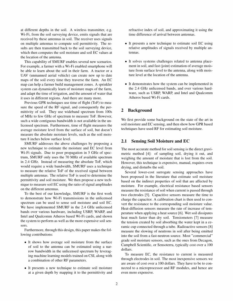
To understand how Wi-Fi frequency bands perform in soilat different moisture levels, we conducted measurementswith a network analyzer in potting soil. Since frequencybelow 1 GHz is known to have good performance in GPRapplications, here our main focus is to look at signal atten-uation at Wi-Fi frequency bands, i.e., 2.4 GHz and 5 GHz.Figure 4 plots the signal attenuation in soil for the three re-ceive antennas at depths of 5 cm, 10 cm and 15 cm in soil.With a transmission power of 15 dBm, the channels mea-sured with smaller than -90 dB log magnitude do not containuseful phase information. We can see that the attenuation at2.4 GHz channels maintain larger than -80 dB log magni-tude at all moisture levels while 5 GHz channels do not havegood signal strength for the bottom antenna even when soilis very dry. Therefore, although 5 GHz channels have a totalbandwidth span of about 665 MHz, the attenuation problemmakes most of the data measured at 5 GHz invalid. Theseresults indicate that we should focus on using 2.4 GHz chan-nels, which have about 70 MHz of available bandwidth.

3.4 Dealing with Multipath

The equations derived in Section 3.1 only consider the short-est path from the transmit to the receive antennas. In prac-tice, channels always consist of multiple paths. In our mea-surement setup, the shortest path is also the strongest path inmost cases. Therefore, we use the MUSIC algorithm to ac-curately recover the shortest path from a multipath channel.

In multipath environment, the CSI of mth antenna and nth

frequency can be written as the sum of L paths

hm,n =L

∑l=1

al,me− j2π( f0+∆ f n)τl,m (22)

where al,m is the complex amplitude of lth path, τl is the

6

2 3 4 5 6−110

−100

−90

−80

−70

−60

−50

−40

−30

−20

−10

Frequency (GHz)

Log m

agnitude o

f channel (d

B)

Channel attenuation over frequencies (depth: 5cm)

Permittivity: 4−7Permittivity: 13−20Permittivity: 15−24Permittivity: 24−34

(a)

2 3 4 5 6−110

−100

−90

−80

−70

−60

−50

−40

−30

−20

−10

Frequency (GHz)

Log m

agnitude o

f channel (d

B)

Channel attenuation over frequencies (depth: 10cm)

Permittivity: 4−7Permittivity: 13−20Permittivity: 15−24Permittivity: 24−34

(b)

2 3 4 5 6−110

−100

−90

−80

−70

−60

−50

−40

−30

−20

−10

Frequency (GHz)

Log m

agnitude o

f channel (d

B)

Channel attenuation over frequencies (depth: 15cm)

Permittivity: 4−7Permittivity: 13−20Permittivity: 15−24Permittivity: 24−34

(c)

Figure 4: Channel attenuation in soil at different depths measured by network analyzer. Generally, signal attenuation increases as frequency,depth, or soil moisture increases.

absolute ToF of lth path and ∆ f is the frequency spacing be-tween two adjacent frequency samples.

If there is no time and frequency synchronization betweenthe transmitter and the receiver, the measured CSI is cor-rupted with packet detection delay (PDD), sampling fre-quency offset (SFO), and carrier frequency offset (CFO) in-troduced by hardware, so the CSI becomes

hm,n =L

∑l=1

al,me− jθ0e− j2π( f0+∆ f n)(τl,m+τ0) (23)

where θ0 is the phase shift caused by CFO and τ0 is theToF shift caused by PDD, SFO, and other possible delays inhardware. θ0 and τ0 are the same across all the paths, sub-carriers in a single channel, and antennas when the samplesare measured at the same time.

Note that although we do not know what τ0 is, we are stillable to get the relative ToF between two antennas, τl,i−τl, j =(τl,i + τ0)− (τl, j + τ0). For a uniform linear antenna array,the path difference remains the same for all adjacent antennapairs under far-field assumption so that the relative ToF alsoremains the same, i.e., ∆τl = τl,i − τl,i+1 = τl,i+1 − τl,i+2.Therefore, we can use MUSIC to jointly estimate absoluteToF (τl,m− τ0) and relative ToF (τl,i− τl, j) in a similar wayas Spotfi [15] did. Here the absolute ToF refers to the to-tal ToF consisting of PDD, SFO, and delays in hardware.However, Spotfi assumes the phase difference caused by theadditional path difference is the the same for all subcarriers,which requires 2πB∆τ to be a small value, where B is the to-tal bandwidth of N subcarriers. This is not true in our systemsince we use a larger bandwidth and look at a longer relativeToF. Considering an antenna array with 3 antennas, we con-struct a modified smoothed CSI matrix without smoothingCSIs of different antennas as follows:

h1,1 h1,2 h1,3 . . . h1,K...

......

. . ....

h1,N−K+1 h1,N−K+2 h1,N−K+3 . . . h1,Nh2,1 h2,2 h2,3 . . . h2,K

......

.... . .

...h2,N−K+1 h2,N−K+2 h2,N−K+3 . . . h2,N

h3,1 h3,2 h3,3 . . . h3,K...

......

. . ....

h3,N−K+1 h3,N−K+2 h3,N−K+3 . . . h3,N

(24)

Resolving Ambiguity in Relative ToF: We first ex-plain the reason for the ambiguity issue and then discuss themethod to remove it. When wave propagates at a carrier fre-quency of f , its phase variation is given by

θ =−2π f τ (25)

where τ is the ToF. The time it takes the phase to rotate2π is τ0 = 1/ f . Assuming that the relative ToF of antennasat different depths is ∆, we get the phase of the three receiveantennas at three depths as: θ1 = −2π f τ , θ2 = −2π f (τ +∆τ) and θ3 = −2π f (τ +2∆τ). Due to phase ambiguity, wehave:

θ1 =−2π f τ

θ2 =−2π f (τ +∆τ) =−2π f (τ +(∆τ + τ0))

=−2π f (τ +(∆τ +2τ0)) = . . .

θ3 =−2π f (τ +2∆τ) =−2π f (τ +2(∆τ + τ0))

=−2π f (τ +2(∆τ +2τ0)) = . . .

(26)

From the above equation, we can see that a delay of ∆τ isequivalent to ∆τ+τ0, ∆τ+2τ0 , . . . . Thus we will get an infi-nite number of possible relative ToF values with a separationof τ0. In 2.4 GHz channels, τ0 is about 0.4 ns.

Next we show how SMURF leverages the knowledge ofsoil properties to remove this ambiguity. First, we know thatthe refraction index in soil is usually between 2 and 6. There-fore, when we set the antenna depth distance at a knownvalue, e.g., 4.5 cm, we know the relative ToF range is 0.3-0.9 ns. In 2.4 GHz, if the relative ToF falls in 0.3-0.5 ns or

7

0.7-0.9 ns, ambiguity occurs. Now recall that in Figure 4, wehave observed a big channel attenuation gap between the twopermittivity ranges corresponding to the two ambiguity val-ues. Although multipath and the rotation of transmit antennamay affect the signal strength, we use the signal strength ofthe three antennas and the data collected at different transmitantenna locations to make a correct choice of antenna pairsto use for relative ToF.

4 Implementation

We implemented SMURF on multiple platforms includingUSRP, WARP, Intel Wi-Fi Link 5300 NIC, and AtherosAR9590 Wi-Fi NIC to measure soil moisture and EC at2.4 GHz. USRP allows us to do wideband experiments forground truthing. The WARP board allows us to replicate CSImeasurements similar to Wi-Fi cards, and microbenchmarkthe performance of SMURF. We validate our results by im-plementing SMURF on two off-the-shelf Wi-Fi cards.

USRP N200 devices with SBX daughterboards can oper-ate on 400-4400 MHz, however, we observe that the trans-mission power of the SBX daughterboards drops as fre-quency increases. Therefore, we only use a bandwidth thatspans from 400 MHz to 1400 MHz in our measurements.We use one USRP device as transmitter and the other as re-ceiver. To emulate a MIMO capable receiver equipped withmultiple antennas as described in Section 3, we switched an-tennas during the measurements. For each antenna, the sys-tem sweeps through the 400-1400 MHz bandwidth with astep size of 5MHz. To allow such an emulation, PLL offsets,CFO, SFO, and PDD should be consistent for all the receiverantennas. We employ two features on USRP to eliminatePLL offsets, CFO and SFO: (i) SBX daughterboards havea PLL phase offset resync feature to synchonize PLL phaseoffsets on two USRPs after each frequency retune; (ii) Twodevices can be connected with a MIMO cable to get time andfrequency synchronization. To reduce the effect of PDD, weuse a narrowband sinusoid to estimate CSI.

WARP boards and the Wi-Fi cards are both MIMO ca-pable and can operate on 2.4 GHz and 5 GHz. With thesetwo types of devices, we consider a more general case thatthe transmitter and receiver do not share oscillators. How toextract valid CSI information from PLL offsets, CFO, SFO,and PDD corrupted CSI data is the key challenge here. TheIntel Wi-Fi cards have a well known issue of random phasejumps at 2.4 GHz [17] while WARP boards and the Atheroscards do not have such an issue. Since WARP has better sup-port for manual configuration, especially gain settings, weevaluated SMURF’s performance mainly with WARP. Weuse a fixed transmit power of 8 dBm in all the experiments,which is much lower than the FCC-imposed power limit for2.4 GHz channels. To investigate the possibility of usingWi-Fi cards to achieve the same performance as WARP, weset the Wi-Fi cards into monitor mode using the open-source

CSI tools[19, 20] on Linux.We use the entire 70 MHz bandwidth at 2.4 GHz spectrum

to cope with potential multipath and amplitude variationsthat occur due to soil heterogeneity and antenna impedancechange. To use the entire bandwidth, we switch acrossthe channels. Therefore, we need to compensate for hard-ware impairments that lead to inconsist measurements acrosschannels. The calibration on WARP has two procedures.First, we calibrate the PLL phase offsets across channels byleveraging a key observation: although PLL phase offsetsare different at different channels, they are constant after afrequency retune. Therefore, the PLL phase offsets at allthe channels can be calibrated at the same time and do notneed re-calibration unless nodes are reset. Then we adoptthe phase sanitization algorithm in SpotFi [15] to equalizethe impact of PDD and SFO on channel phase slopes acrossmultiple channel measurements. For Wi-Fi cards, since theRF chains share the same PLL, their random phase behaviouris simpler than WARP, which only has two possible statesseparated by π .

(a) (b) (c)

Figure 5: Soil measurement setup for multi-antenna system. An-tennas are at different depths in soil while there is a rod coming outfrom soil surface to indicate the location of antenna array in soil. (a)Antennas protected by a waterproof box. (b) Tent with soil boxes.(c) Measurement setup on a farm.

As depicted in Figure 5, we use a waterproof box to pro-tect the connectors of antennas as well as hold antennas atdifferent depths in soil, and there is a rod coming out fromsoil surface to tell the farmers where the antennas are buried.We setup potting soil boxes in a tent to conduct measure-ments with controlled salinity and moisture levels, and testreal soils in outdoor environments.

5 Performance Evaluation

We first show the accuracy of SMURF in measuring relativeToF, and then evaluate its performance in measuring soil per-mittivity, EC, and moisture. We use wideband USRP to mea-sure ground truth, and Wi-Fi based measurements on WARPto microbenchmark SMURF. We also present results usingIntel and Atheros Wi-Fi cards.

5.1 Relative ToF Estimation AccuracySMURF is able to accurately estimate soil moisture and ECwith limited bandwidth in 2.4 GHz Wi-Fi. Here we show that

8

0 0.1 0.2 0.3 0.4 0.5 0.60

0.5

1

1.5

2

2.5

3

3.5

Rx Antenna distance (m)

Rela

tive T

OF

(ns)

Joint relative TOF estimation with different bandwidth

Bandwidth: 50MHz (520MHz−570MHz)Bandwidth: 100MHz (520MHz−620MHz)Bandwidth: 230MHz (470MHz−700MHz)Bandwidth: 500MHz (400MHz−900MHz)Bandwidth: 1GHz (400MHz−1400MHz)Ground truth

(a)

0 0.1 0.2 0.3 0.4 0.5 0.60

5

10

15

Rx Antenna distance (m)

Absolu

te T

OF

(ns)

Joint absolute TOF estimation with different bandwidth

Bandwidth: 50MHz (520MHz−570MHz)Bandwidth: 100MHz (520MHz−620MHz)Bandwidth: 230MHz (470MHz−700MHz)Bandwidth: 500MHz (400MHz−900MHz)Bandwidth: 1GHz (400MHz−1400MHz)Ground truth

(b)

0 200 400 600 800 1000

0

1

2

3

4

5

6

Bandwidth (MHz)

MS

E (

ns)

MSE of relative TOF estimation at different Rx antenna distances

Separate estimation

Joint estimation

(c)

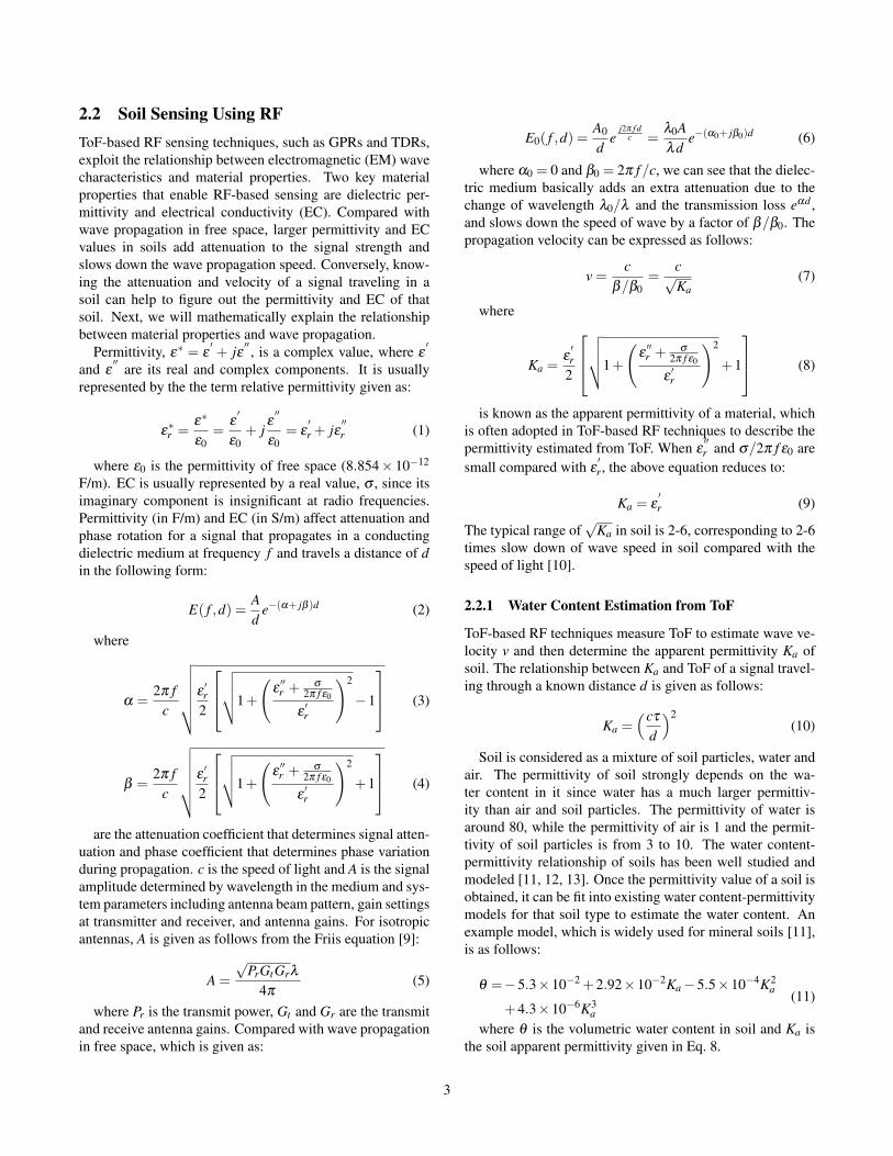
Figure 6: Performance of the multi-antenna system in estimating relative ToF. (a) Joint relative ToF estimation. Using 3 antennas to jointlyestimate relative ToF and absolute ToF give very accurate results even with small bandwidth.(b) Joint absolute ToF estimation for the antennaclosest to the transmit antenna. Smaller bandwidth deviates more in estimating absolute ToF. (c) MSE of relative ToF estimation with differentbandwidth. The joint estimation method outperforms separate estimation at small bandwidth.

0 2 4 6 8

10

15

20

25

30

35

40

Antenna depth difference (cm)

Appare

nt die

lectr

ic p

erm

ittivity

Soil permittivity estimation with different antenna depth difference

Permittivity range measured by soil sensorBandwidth: 50MHz (520MHz−570MHz)Bandwidth: 100MHz (520MHz−620MHz)Bandwidth: 230MHz (470MHz−700MHz)Bandwidth: 500MHz (400MHz−900MHz)Bandwidth: 1GHz (400MHz−1400MHz)

(a)

1 2 3 40

20

40

60

80

100

Moisture level

Appare

nt die

lectr

ic p

erm

ittivity

Soil permittivity estimation at different moisture levels

Permittivity range measured by soil sensorBandwidth: 50MHz (520MHz−570MHz)Bandwidth: 100MHz (520MHz−620MHz)Bandwidth: 230MHz (470MHz−700MHz)Bandwidth: 500MHz (400MHz−900MHz)Bandwidth: 1GHz (400MHz−1400MHz)

(b)

1 2 3 4 50

10

20

30

40

50

Moisture level

Appare

nt die

lectr

ic p

erm

ittivity

Soil permittivity estimation at different moisture levels

Permittivity range measured by soil sensor

2.4GHz channels with 70MHz bandwidth

(c)

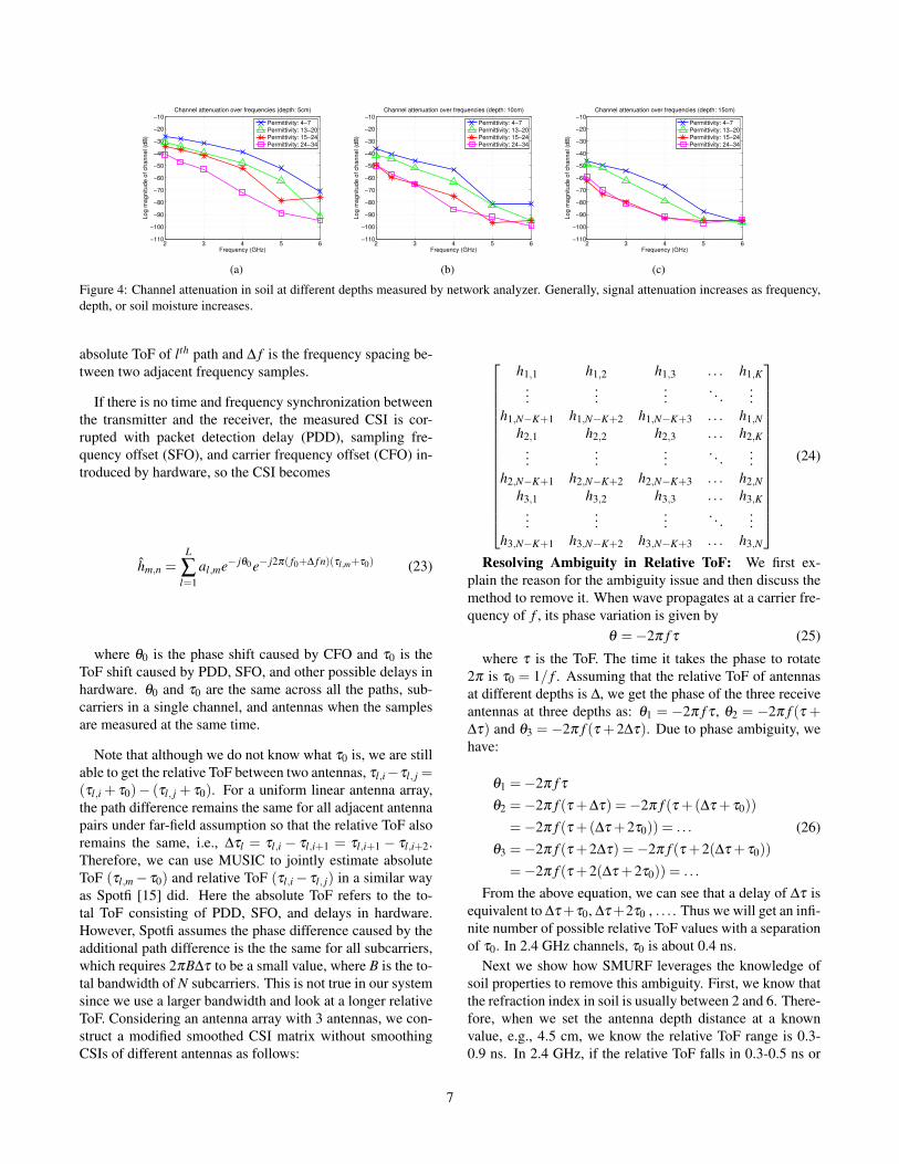
Figure 7: Soil dielectric permittivity estimation based on relative ToF. (a) Permittivity estimation from USRPs with different antenna depthdifferences. A small depth difference results in large estimation error. (b) Permittivity estimation with USRPs at different moisture levels.The system can accurately estimate soil moisture value at all soil moisture levels. Even a small bandwidth performs well in distinguishingsoil moisture levels. (c) Permittivity estimation with WARPs at different moisture levels. Permittivity estimated from 2.4 GHz channels isgenerally smaller than the sensor data.

with a few antennas at the receiver, the relative ToF estima-tion is very accurate even with a very small bandwidth. Wefirst use USRP over a large bandwidth to micro-benchmark,and then use WARP to evaluate the performance at 2.4 GHzchannels.

5.1.1 Time-of-Flight Accuracy over the Air

Soil is not a homogeneous medium, and its variations canintroduce shifts in estimated ToF. Therefore, we use over-the-air measurements to evaluate the system’s performancein estimating absolute ToF. The ground truth ToF is the dis-tance of antennas measured by tape measure and divided byspeed of light. We conducted measurements with USRPs byvarying the distance between adjacent receive antennas from0.1 m to 0.5 m. The distance between the transmit antennaand the receive antenna closest to it is 1.2 m and remains thesame across all the measurements.

Figure 6 plots the relative ToF and absolute ToF estimationresults given by the joint estimation method and the separateestimation method. Relative ToF refers to the ToF differ-ence between two adjacent antennas. The separate estima-tion method refers to first estimating absolute ToFs at the

three antennas separately from the CSI collected by the threereceive antennas and then calculating the relative ToF fromthe average difference of absolute ToFs. The joint estima-tion method estimates relative ToF and absolute ToF at thesame time for the three antennas. Surprisingly, with the jointestimation method, even a bandwidth of 50 MHz gives accu-rate relative ToF results, although its absolute ToF estimationcan deviate more from the ground truth. Furthermore, thejoint estimation method has a much smaller MSE of relativeToF and absolute ToF estimation than the separate estimationwith small bandwidth.

5.1.2 Relative Time-of-Flight Accuracy in soil

Here we examine the relative ToF estimation performance ofthe multi-antenna system in soil. We conducted the exper-iments in potting soil in indoor environment. In the USRPexperiments, the transmit antenna is set at a height of 1.08mabove soil surface, the receive antennas are put at differentdepths in soil. In the WARP experiments, the transmit an-tenna is 0.36m above soil surface. We compare our resultswith the permittivity measured by a Decagon GS3 soil sen-sor, which can simultaneous measure permittivity, EC and

9

temperature. In each experiment, we use the soil sensorto measure moisture at more than 10 locations in the areaaround the antenna array to account for heterogeneity of soil.

Impact of antenna depth separation: As discussedin 3.3.1, the choice of antenna depth separation is the keyfactor that affects the relative ToF estimation accuracy in ourantenna array design. We conducted experiments with US-RPs to examine the impact of depth difference. Figure 7(a)plots the permittivity estimated from relative ToF when an-tennas have different depth separation. Sensor data showsthat soil moisture can vary within a certain range in an area.With a depth separation of 1.5 cm, the estimated permittivitycan deviate a lot from sensor data. The reason is the depthseparation of 1.5 cm is relatively small compared to possiblepath length variations that exist in soil due to the heteroge-neous nature of soil. With larger antenna depth separation,the permittivity values estimated by different bandwidth aremore converged.Based on the results shown in Figure 7(a),we choose an antenna depth separation of 4.5 cm to evalu-ate the performance of USRP and WARP in the followingdiscussions.

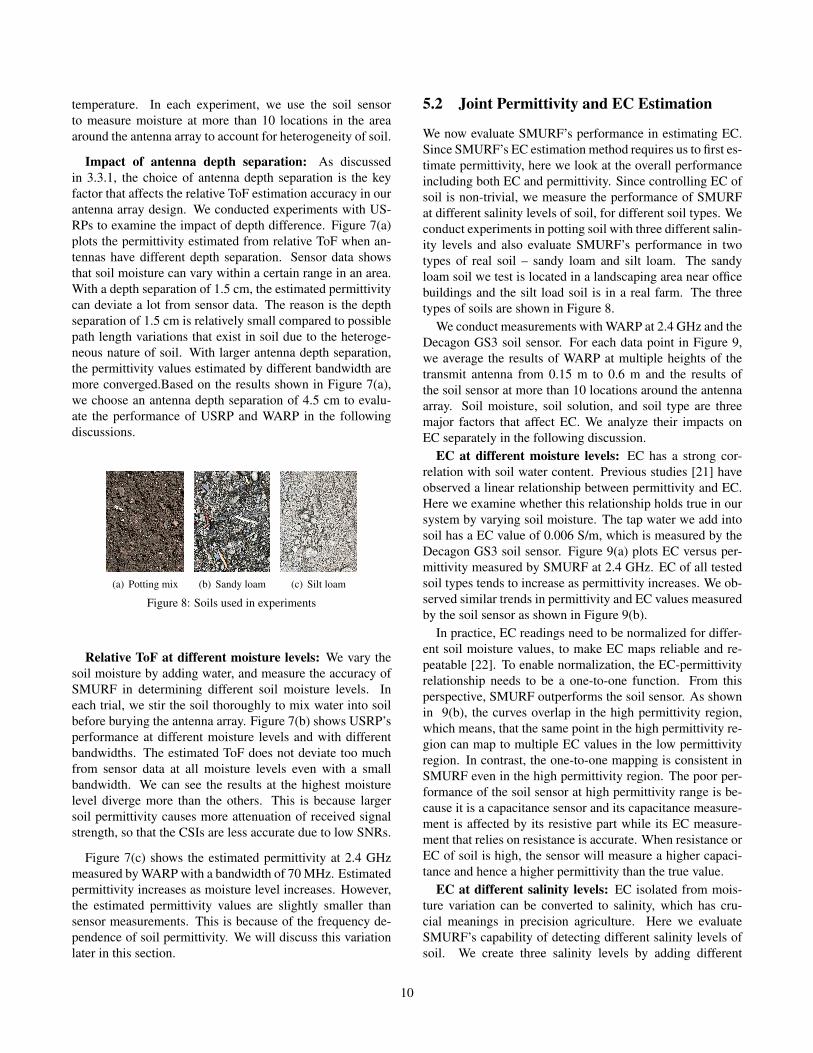
(a) Potting mix (b) Sandy loam (c) Silt loam

Figure 8: Soils used in experiments

Relative ToF at different moisture levels: We vary thesoil moisture by adding water, and measure the accuracy ofSMURF in determining different soil moisture levels. Ineach trial, we stir the soil thoroughly to mix water into soilbefore burying the antenna array. Figure 7(b) shows USRP’sperformance at different moisture levels and with differentbandwidths. The estimated ToF does not deviate too muchfrom sensor data at all moisture levels even with a smallbandwidth. We can see the results at the highest moisturelevel diverge more than the others. This is because largersoil permittivity causes more attenuation of received signalstrength, so that the CSIs are less accurate due to low SNRs.

Figure 7(c) shows the estimated permittivity at 2.4 GHzmeasured by WARP with a bandwidth of 70 MHz. Estimatedpermittivity increases as moisture level increases. However,the estimated permittivity values are slightly smaller thansensor measurements. This is because of the frequency de-pendence of soil permittivity. We will discuss this variationlater in this section.

5.2 Joint Permittivity and EC Estimation

We now evaluate SMURF’s performance in estimating EC.Since SMURF’s EC estimation method requires us to first es-timate permittivity, here we look at the overall performanceincluding both EC and permittivity. Since controlling EC ofsoil is non-trivial, we measure the performance of SMURFat different salinity levels of soil, for different soil types. Weconduct experiments in potting soil with three different salin-ity levels and also evaluate SMURF’s performance in twotypes of real soil – sandy loam and silt loam. The sandyloam soil we test is located in a landscaping area near officebuildings and the silt load soil is in a real farm. The threetypes of soils are shown in Figure 8.

We conduct measurements with WARP at 2.4 GHz and theDecagon GS3 soil sensor. For each data point in Figure 9,we average the results of WARP at multiple heights of thetransmit antenna from 0.15 m to 0.6 m and the results ofthe soil sensor at more than 10 locations around the antennaarray. Soil moisture, soil solution, and soil type are threemajor factors that affect EC. We analyze their impacts onEC separately in the following discussion.

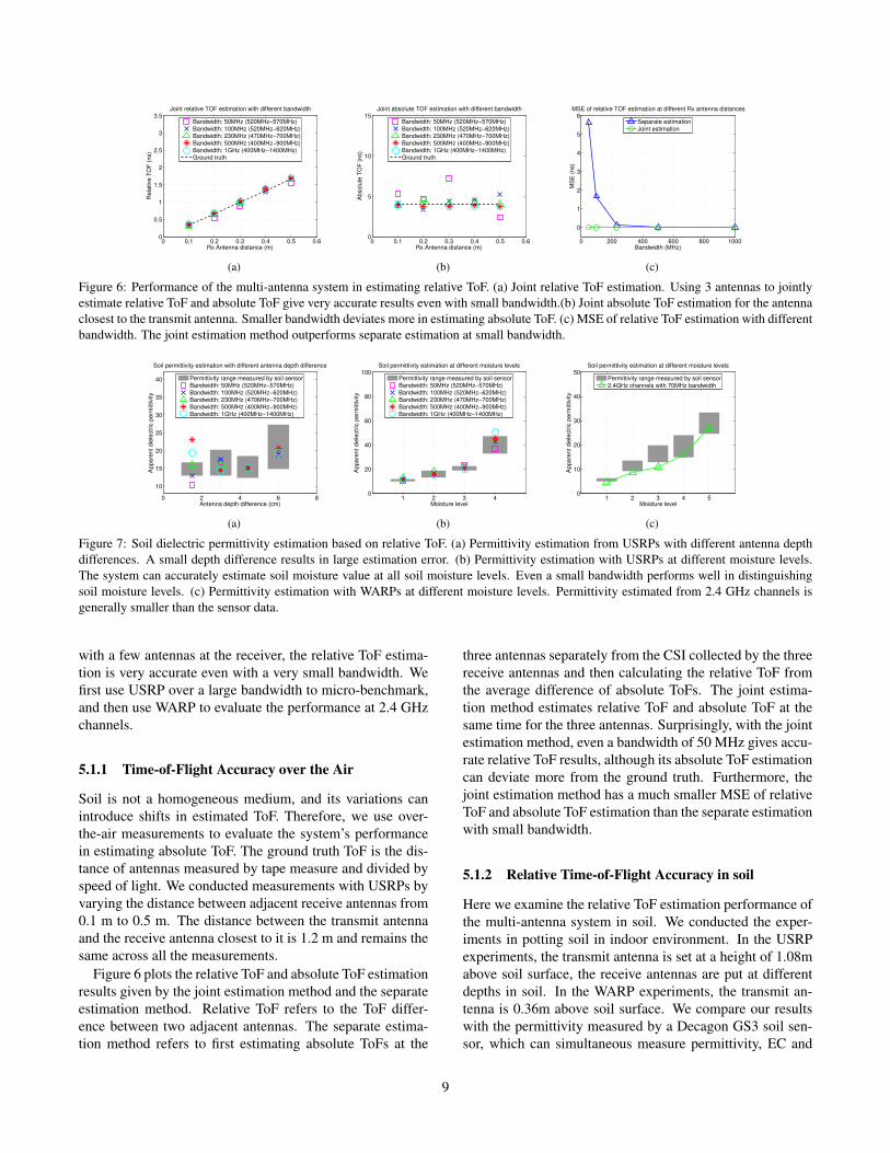
EC at different moisture levels: EC has a strong cor-relation with soil water content. Previous studies [21] haveobserved a linear relationship between permittivity and EC.Here we examine whether this relationship holds true in oursystem by varying soil moisture. The tap water we add intosoil has a EC value of 0.006 S/m, which is measured by theDecagon GS3 soil sensor. Figure 9(a) plots EC versus per-mittivity measured by SMURF at 2.4 GHz. EC of all testedsoil types tends to increase as permittivity increases. We ob-served similar trends in permittivity and EC values measuredby the soil sensor as shown in Figure 9(b).

In practice, EC readings need to be normalized for differ-ent soil moisture values, to make EC maps reliable and re-peatable [22]. To enable normalization, the EC-permittivityrelationship needs to be a one-to-one function. From thisperspective, SMURF outperforms the soil sensor. As shownin 9(b), the curves overlap in the high permittivity region,which means, that the same point in the high permittivity re-gion can map to multiple EC values in the low permittivityregion. In contrast, the one-to-one mapping is consistent inSMURF even in the high permittivity region. The poor per-formance of the soil sensor at high permittivity range is be-cause it is a capacitance sensor and its capacitance measure-ment is affected by its resistive part while its EC measure-ment that relies on resistance is accurate. When resistance orEC of soil is high, the sensor will measure a higher capaci-tance and hence a higher permittivity than the true value.

EC at different salinity levels: EC isolated from mois-ture variation can be converted to salinity, which has cru-cial meanings in precision agriculture. Here we evaluateSMURF’s capability of detecting different salinity levels ofsoil. We create three salinity levels by adding different

10

0 5 10 15 20 25 30 350

0.2

0.4

0.6

0.8

1

1.2

1.4

Permittivity

EC

(S/m

)Permittivity and EC measured by WARP

Sandy loamSilt loamPotting (salinity level 1)Potting (salinity level 2)Potting (salinity level 3)

(a)

0 10 20 30 40 500

0.05

0.1

0.15

0.2

0.25

0.3

0.35

0.4

Permittivity

EC

(S/m

)

Permittivity and EC measured by soil sensor

Sandy loamSilt loamPotting (salinity level 1)Potting (salinity level 2)Potting (salinity level 3)

(b)

0 0.05 0.1 0.15 0.2 0.25 0.30

0.2

0.4

0.6

0.8

1

1.2

1.4

EC from sensor (S/m)

EC

fro

m W

AR

P (

S/m

)

EC measured by soil sensor and WARP

Sandy loamSilt loamPotting (salinity level 1)Potting (salinity level 2)Potting (salinity level 3)

(c)

0 10 20 30 40 500

10

20

30

40

50

60

Permittivity from sensor

Perm

ittivity fro

m W

AR

P

Permittivity measured by soil sensor and WARP

Sandy loamSilt loamPotting (salinity level 1)Potting (salinity level 2)Potting (salinity level 3)

(d)

Figure 9: Soil permittivity and EC estimation for different soil types and salinity levels. (a) Permittivity and EC measured by WARP with 2.4GHz channels. EC increases as moisture level increases and salinity level increases. (b) Permittivity and EC measured by soil sensor at 70MHz. EC level affects the soil sensor’s permittivity estimation accuracy. (c) Comparison between EC measured by soil sensor and WARP. ECmeasured at 2.4 GHz is higher than EC measured by soil sensor. (d) Comparison between permittivity measured by soil sensor and WARP.WARP results of different soil types deviate from the soil sensor differently. The deviation is larger at higher salinity levels.

0 500 1000 1500 2000 250010

15

20

25

30

35

40

45

50

55

Frequency (MHz)

Pe

rmittivity

Permittivity measured at different frequencies

Wetter soil Dryer soil

Soil sensor USRP WARP

(a)

0 500 1000 1500 2000 25000

0.2

0.4

0.6

0.8

1

Frequency (MHz)

EC

(S

/m)

EC measured at different frequencies

Wetter soil Dryer soil

Soil sensor USRP WARP

(b)

0 500 1000 1500 2000 25000

10

20

30

40

50

60

70

Frequency (MHz)

Imagin

ary

perm

ittiiv

ty

Imaginary part of permittivity measured at different frequencies

Wetter soil Dryer soil

Soil sensor USRP WARP

(c)

Figure 10: Permittivity and EC measured by soil sensor, USRP and WARP at different frequencies. (a) Apparent permittivty drops asfrequency increases. (b) EC increases as frequency increases. (c) Imaginary effective permittivity converted from EC.

amount of salt into three boxes with the same type of pot-ting soil. By looking at EC values vertically with the samepermittivity in Figure 9(a) and Figure 9(b), we observe thatSMURF can successfully detect the increase of salinity lev-els from EC readings at all permittivity regions while the soilsensor can only tell the difference of salinity levels when per-mittivity is smaller than 20.

EC in different soils: Different soil types may have dif-ferent EC-permittivity and EC-salinity relationships due todielectric property change [23]. Previously, we conductedmost of our experiments with potting soil since it is more ac-cessible and hence easier to set up controlled experiments.Here we test two typical types of real soils to show the ac-curacy of SMURF in detecting permittivity and EC of realworld soils. As shown in Figure 9(a) and Figure 9(b), thethree types of soils have quite different salinity levels. Gen-erally, SMURF can detect the permittivity increase as watercontent increases and EC increase as salinity level increasesin different types of soils. The rate of increase in EC overpermittivity is different for different soil types and even forthe same soil type with different salinity levels. In practice,SMURF will need to be calibrated for different soil types,just as the existing soil sensors have to be calibrated beforeuse.

Comparing SMURF with soil sensor: We plot EC mea-sured by SMURF and the soil sensor in Figure 9(c), and

permittivity measured by SMURF and the soil sensor inFigure 9(d). Overall, SMURF measures a larger EC valueand a smaller permittivity value than the soil sensor. TheEC-EC slopes decrease as salinity level increases while thepermittivity-permittivity slopes do not have a clear trend.The permittivity deviation is larger at larger moisture levels.

Comparing WARP with Atheros Wi-Fi card: To com-pare the performance of WARP and Atheros Wi-Fi card, weconduct experiments with the same transmit and receive an-tenna locations for same soil. Basically, we just change thedata transmit and record devices from WARPs to AtherosWiFi cards. We see very similar CSI phase results measuredby WARP and Wi-Fi cards. While the Atheros Wi-Fi cardsdo not give reliable amplitude measurements, we can use itsRSSI reported for each channel for EC estimation. We ob-serve that the EC measured by Wi-Fi cards using RSSIs aresimilar to the EC measured by WARP. One example set ofresults is: permittivity and EC measured by WARP is 8.8and 0.24 S/m, while permittivity and EC measured by Wi-Fiis 9.2 and 0.21 S/m.

5.2.1 Understanding Permittivity and EC Deviationsbetween SMURF and Soil Sensor

Previous studies [8, 23, 24, 25] show that both the real andimaginary parts of permittivity of soil are frequency depen-

11

dent and affected by salinity, where the imaginary permit-tivity refers to the effective imaginary permittivity given asε′′re = ε

′′r + σ/2π f ε0. In the frequency range from a few

MHz to Wi-Fi frequency bands at 2.4 GHz, the real andimaginary parts of permittivity both drop over frequencywhile the imaginary drops more significantly at lower fre-quencies. As salinity increases, the real permittivity slightlydrops while the imaginary permittivity increases and the in-crease is significant at lower frequencies. The difference ofimaginary permittivity at lower frequencies and higher fre-quencies is due to the EC component σ/2π f ε0. To evalu-ate how SMURF’s relative ToF and relative amplitude basedpermittivity and EC estimation match with existing studies,we conduct experiments with the soil sensor operating at 70MHz, USRP operating at 400-1400 MHz, and WARP op-erating at 2.402-2.472 GHz. Both USRP and WARP use themulti-antenna system to measure relative ToF and amplitude.Since USRP measures a wide bandwidth, we are able to getmultiple data points by selecting subsets of frequency rangeswithin 400-1400 MHz.

Figure 10 shows the results of potting soil at two differ-ent moisture levels. As frequency increases, the estimatedpermittivity decreases and EC increases, which agree withthe deviations we observe earlier. Note that effective imag-inary and effective EC, which is the EC value we measure,are two interchangeable concepts and has a relationship ofε′′re = σa/2π f ε0. We convert our EC results to imaginary

permittivity in Figure 10(c) for a more intuitive comparisonwith exiting studies. The trends and scale of values of ourestimated real and imaginary permittivity match with resultsreported in [25].

Implications for calibration requirements: The aboveanalysis provides implications about how we should cali-brate our system. (i) Getting real part of permittivity fromapparent permittivity measurement: as we can see from Fig-ure 10(c), the imaginary permittivity at 2.4 GHz is a smallvalue compared with the real part of permittivity so the mea-sured apparent permittivity is equal to the real part of permit-tivity and there is no need for calibration. (ii) Estimating soilwater content from permittivity: the drop of real permittiv-ity over frequency needs to be calibrated to use the existingwater content-permittivity models which are mainly devel-oped for lower frequencies. Fortunately, the dependence ofreal and imaginary permittivity on frequency has been mod-eled for different soil types, although measurements are stillrequired to validate those models. (iii) Estimating salinityfrom measured EC: to get the true EC component, the imag-inary permittivity component needs to be removed from themeasured apparent EC. On the one hand, we can refer to ex-isting studies of soil dielectric properties to get the imaginarypermittivity values for different soil types; on the other hand,our results in Figure 9(a) and 9(c) indicate that it is possibleto directly convert our measured EC to salinity.

6 Related Work

While soil sensing using RF has been well studied, our workis the first that makes it possible to use off-the-shelf low-cost Wi-Fi devices for detecting soil properties. We discussrelated work in three main categories:

Soil moisture sensing using RF: The well-establishedRF sensing techniques can be classified into three types. (i)Remote sensing techniques[26, 27, 28] use the dependenceof soil reflectivity on soil moisture to sense soil moisture.These approaches have low spatial resolution from 1 m to10s of km and can only detect soil moisture on shallow soilsurface with a depth of a few centimeters. (ii) ToF-basedtechniques such as GPR [29] and time domain reflectometry(TDR) [30] provides good spatial resolution. However, theseapproaches rely on specialized ultra-wideband systems to getaccurate ToF estimation, thus are very expensive. (iii) A fewstudies [31, 32, 33, 34] have proposed to use a moisture orEC sensitive sensing element together with a low-cost com-munication node, e.g., RFID or backscatter, to sense soil.However, low-cost sensing elements like a capacitive sensorcan only sensor moisture, not EC, and its accuracy will notbe comparable to the more reliable but higher-cost commod-ity sensors. A specialized probe that is sensitive to moistureand salinity change is used in [32] to detect moisture andsalinity, which could potentially increase cost.

AoA and ToF estimation on Wi-Fi devices: We buildSMURF on existing AoA and ToF estimation technologiesdeveloped for commodity Wi-Fi devices [15, 35, 36, 20, 16,37]. However, these technologies do not work for wave prop-agation in soil due to different reasons. The sub-nanosecondaccuracy achieved in Chronos [35] is unlikely in soil due tothe high attenuation of 5 GHz signals. SpotFi’s [35] accuracybenefits from 40 MHz bandwidth and the carrier frequencyof 5 GHz. To combat signal attenuation in soil, we insteaduse 20 MHz channels at 2.4GHz. To deal with multipath insoil and amplitude variations due to impedance change orsoil heterogeneity, we spliced all 2.4 GHz channels. How-ever, existing work on channel splicing only works for asingle antenna [20, 37]. We utilize our observations abouthardware to eliminate exhaustive search for both PLL phaseoffset calibration [17] and channel splicing [20, 37]

Other low-cost techniques: Other than ultra-widebandsystems and Wi-Fi devices, there are some other commer-cially available RF devices that can provide ToF estimation,such as global positioning system (GPS) receivers [38]. GPSrelies on ToF between satellites and the receiver for localiza-tion. However, its ToF resolution and penetration depth limitits usage in ToF-based soil moisture sensing. Ranging tech-niques using ultrasound [39, 40] have been well studied forover the air wave propagation. However, ultrasound is notappropriate for ToF-based soil moisture estimation since itdoes not correlate very with moisture, which limits its appli-cations of soil sensing to rely on reflectivity[41, 42].

12

Although there exist hobbyist soil sensors that cost lowerthan 30 dollars, they are not recommended by agricultureexperts for irrigation management on farms [2]. The cheap-est suggested soil moisture sensors still cost over 50 dollars.Actually, the higher accuracy of expensive sensors can po-tentially help to save more water resources in the long term.We note that we are not aware of any commercially availableEC sensor below 100 dollars.

7 Discussion & Future Work

SMURF takes the first step in leveraging Wi-Fi communica-tion for estimating soil properties. However, for it to achieveits true potential, where a farmer with any Wi-Fi enabled de-vice can infer soil properties, we plan to take SMURF in thefollowing directions.

Integration with commercial Wi-Fi devices: The Wi-Fichip vendors in off-the-shelf phones have started to exposeCSI information. The Intel and Atheros 11n chipsets haveshown the feasibility of providing this information to the userlevel, and we will work with other chip vendors to exposethese values. We note that SMURF only requires a singleantenna at the smartphone. Furthermore, since 2.4 GHz ofthe spectrum is available in nearly all countries, we expectSMURF to be universally usable.

Profiling overhead: In its current implementationSMURF relies on an offline profiling of the ToF and relativeToF values for different soil types. This is similar to how sur-rogate soil sensing methods are currently used. We howeverrealize that this is an overhead when using these sensors, andcould potentially be a source of inaccuracy in unknown soilconditions. We are investigating ways in which the multipleantennas in soil can be used to self calibrate, especially sinceeach pair of antennas can be used as a different measurementto estimate the corresponding soil type.

Sensing deeper in soil: The technique might not workover 2.4 GHz of spectrum for fruit orchards, where the rootsmight be up to 1 meter deep, and the Wi-Fi signals might nothave good SNR at those depths. TV white space spectrumcan be used to sense soil at depths deeper than 1 m, whichis sufficient for most broadacre crops and for horticulture.While one could still use SMURF over the TV White Spacespectrum, we are investigating ways in which Wi-Fi over the2.4 GHz spectrum could be used as well. Our key insightis to use beamforming to increase the SNR in the directionof the antennas in soil. The challenge of course is that thedirection of the beamformed signal will have to change basedon the moisture level of soil. We are actively investigatingsolutions to this problem.

Price: We note that SMURF does not require a special-ized reader. Only a Wi-Fi device is needed to communicatewith the device embedded in soil. For the device in soil, itis recommended to use a chipset with 3 antennas, althougha 2-antenna radio can work as well. The price of a typical

IoT board with a Wi-Fi chipset with an onboard ARM pro-cessor and batteries is similar to a Vocore2, or C.H.I.P., bothof which cost less than 10 dollars.

Battery Life: The device in soil only needs to wake upwhen the surveying device is closeby. Else, it should operatein deep sleep mode. One way to accomplish this is usingthe Network List Offload (NLO) feature of Wi-Fi that turnsthe radio into very low power mode until it hears a beaconwith the expected BSSID. In this case, the surveyor can beprogrammed to pretend like a Wi-Fi Access Point and emit abeacon with a SMURF BSSID.

8 Summary

In this paper we present a new technique, called SMURF,for estimating soil moisture and EC using Wi-Fi signals. Thesystem estimates soil moisture by measuring the relative timeof flight of Wi-Fi between multiple antennas, and the soilEC by measuring the ratios of the amplitudes of the signalsacross different antennas. We have implemented SMURFon two different SDR platforms, and on two Wi-Fi cards.Our results show that SMURF can accurately estimate soilmoisture and EC at various depths.

Our vision is to enable a future in which a farmer can takeher smartphone, which has a Wi-Fi radio, close to soil andlearns about the soil conditions, such as soil moisture andsoil EC. By avoiding use of sensors that cost more than 100sof dollars each, SMURF reduces the price for sensing theseparameters, thereby taking a big step in enabling the adop-tion of data-driven agriculture techniques by small holderfarmers.

References

[1] Soil electrical conductivity, soil quality kit – guide foreducators, usda nrcs.

[2] Soil moisture monitoring: a selection guide, depart-ment of primary industries and regional development,government of australia, 5th sep, 2018.

[3] Deepak Vasisht, Zerina Kapetanovic, Jongho Won,Xinxin Jin, Ranveer Chandra, Sudipta N. Sinha, AshishKapoor, Madhusudhan Sudarshan, and Sean Stratman.Farmbeats: An iot platform for data-driven agricul-ture. In 14th USENIX Symposium on Networked Sys-tems Design and Implementation, NSDI 2017, Boston,MA, USA, March 27-29, 2017, pages 515–529, 2017.

[4] Milton Whitney et al. Instructions for taking samplesof soil for moisture determinations. 1894.

[5] EA Colman. The place of electrical soil-moisture me-ters in hydrologic research. Eos, Transactions Ameri-can Geophysical Union, 27(6):847–853, 1946.

13

[6] Harrison E Patten. Heat transference in soils. 1909.

[7] LA Richards. Soil moisture tensiometer materials andconstruction. Soil Sci, 53(4):241–248, 1942.

[8] Wilford Gardner and Don Kirkham. Determinationof soil moisture by neutron scattering. Soil Science,73(5):391–402, 1952.

[9] Harald T Friis. A note on a simple transmission for-mula. Proceedings of the IRE, 34(5):254–256, 1946.

[10] Harry M Jol. Ground penetrating radar theory and ap-plications. elsevier, 2008.

[11] G Clarke Topp, JL Davis, and Aa P Annan. Electro-magnetic determination of soil water content: Mea-surements in coaxial transmission lines. Water re-sources research, 16(3):574–582, 1980.

[12] Kurt Roth, Rainer Schulin, Hannes Fluhler, and WernerAttinger. Calibration of time domain reflectome-try for water content measurement using a compos-ite dielectric approach. Water Resources Research,26(10):2267–2273, 1990.

[13] John O Curtis. Moisture effects on the dielectric prop-erties of soils. IEEE transactions on geoscience andremote sensing, 39(1):125–128, 2001.

[14] DA Robinson, Scott B Jones, JM Wraith, Daniel Or,and SP Friedman. A review of advances in dielec-tric and electrical conductivity measurement in soils us-ing time domain reflectometry. Vadose Zone Journal,2(4):444–475, 2003.

[15] Manikanta Kotaru, Kiran Joshi, Dinesh Bharadia, andSachin Katti. Spotfi: Decimeter level localization usingwifi. In ACM SIGCOMM Computer CommunicationReview, volume 45, pages 269–282. ACM, 2015.

[16] Jie Xiong and Kyle Jamieson. Arraytrack: a fine-grained indoor location system. Usenix, 2013.

[17] Jon Gjengset, Jie Xiong, Graeme McPhillips, and KyleJamieson. Phaser: Enabling phased array signal pro-cessing on commodity wifi access points. In Pro-ceedings of the 20th annual international conferenceon Mobile computing and networking, pages 153–164.ACM, 2014.

[18] ZHI Sun, Ian F Akyildiz, and Gerhard P Hancke. Dy-namic connectivity in wireless underground sensor net-works. IEEE Transactions on Wireless Communica-tions, 10(12):4334–4344, 2011.

[19] Daniel Halperin, Wenjun Hu, Anmol Sheth, and DavidWetherall. Tool release: Gathering 802.11 n traces withchannel state information. ACM SIGCOMM ComputerCommunication Review, 41(1):53–53, 2011.

[20] Yaxiong Xie, Zhenjiang Li, and Mo Li. Precise powerdelay profiling with commodity wifi. In Proceedingsof the 21st Annual International Conference on MobileComputing and Networking, pages 53–64. ACM, 2015.

[21] MA Hilhorst. A pore water conductivity sensor. SoilScience Society of America Journal, 64(6):1922–1925,2000.

[22] Robert Dwight Grisso, Marcus M Alley, David LeeHolshouser, and Wade Everett Thomason. Precisionfarming tools. soil electrical conductivity. 2005.

[23] Myron C Dobson, Fawwaz T Ulaby, Martti T Hal-likainen, and Mohamed A El-Rayes. Microwave di-electric behavior of wet soil-part ii: Dielectric mixingmodels. IEEE Transactions on Geoscience and RemoteSensing, (1):35–46, 1985.

[24] M Craig Dobson and Fawwaz T Ulaby. Active mi-crowave soil moisture research. IEEE Transactions onGeoscience and Remote Sensing, (1):23–36, 1986.

[25] Timo Saarenketo. Electrical properties of water in clayand silty soils. Journal of Applied Geophysics, 40(1-3):73–88, 1998.

[26] JR Wang and BJ Choudhury. Remote sensing ofsoil moisture content, over bare field at 1.4 ghz fre-quency. Journal of Geophysical Research: Oceans,86(C6):5277–5282, 1981.

[27] Thomas J Jackson. Iii. measuring surface soil moistureusing passive microwave remote sensing. Hydrologicalprocesses, 7(2):139–152, 1993.

[28] Binayak P Mohanty, Michael H Cosh, Venkat Lak-shmi, and Carsten Montzka. Soil moisture remote sens-ing: State-of-the-science. Vadose Zone Journal, 16(1),2017.

[29] JA Huisman, SS Hubbard, JD Redman, and AP Annan.Measuring soil water content with ground penetratingradar. Vadose zone journal, 2(4):476–491, 2003.

[30] K Noborio. Measurement of soil water content andelectrical conductivity by time domain reflectometry:a review. Computers and electronics in agriculture,31(3):213–237, 2001.

[31] Azhar Hasan, Rahul Bhattacharyya, and Sanjay Sarma.A monopole-coupled rfid sensor for pervasive soilmoisture monitoring. In Antennas and Propagation So-ciety International Symposium (APSURSI), 2013 IEEE,pages 2309–2310. IEEE, 2013.

14

[32] Shuvashis Dey, Nemai Karmakar, Rahul Bhat-tacharyya, and Sanjay Sarma. Electromagnetic charac-terization of soil moisture and salinity for uhf rfid ap-plications in precision agriculture. In Microwave Con-ference (EuMC), 2016 46th European, pages 616–619.IEEE, 2016.

[33] Spyridon-Nektarios Daskalakis, Stylianos D Assimo-nis, Eleftherios Kampianakis, and Aggelos Bletsas.Soil moisture scatter radio networking with low power.IEEE Transactions on Microwave Theory and Tech-niques, 64(7):2338–2346, 2016.

[34] Md Mazidul Islam, Kimmo Rasilainen, and Ville Vi-ikari. Implementation of sensor rfid: Carrying sen-sor information in the modulation frequency. IEEETransactions on Microwave Theory and Techniques,63(8):2672–2681, 2015.

[35] Deepak Vasisht, Swarun Kumar, and Dina Katabi.Decimeter-level localization with a single wifi accesspoint. In NSDI, pages 165–178, 2016.

[36] Swarun Kumar, Stephanie Gil, Dina Katabi, andDaniela Rus. Accurate indoor localization with zerostart-up cost. In Proceedings of the 20th annual in-ternational conference on Mobile computing and net-working, pages 483–494. ACM, 2014.

[37] Jie Xiong, Karthikeyan Sundaresan, and KyleJamieson. Tonetrack: Leveraging frequency-agileradios for time-based indoor wireless localization.In Proceedings of the 21st Annual InternationalConference on Mobile Computing and Networking,pages 537–549. ACM, 2015.

[38] Elliott Kaplan and Christopher Hegarty. UnderstandingGPS: principles and applications. Artech house, 2005.

[39] Andy Ward, Alan Jones, and Andy Hopper. A newlocation technique for the active office. IEEE Personalcommunications, 4(5):42–47, 1997.

[40] Nissanka B Priyantha, Anit Chakraborty, and Hari Bal-akrishnan. The cricket location-support system. InProceedings of the 6th annual international conferenceon Mobile computing and networking, pages 32–43.ACM, 2000.

[41] DA Robinson, CS Campbell, JW Hopmans, Brian KHornbuckle, Scott B Jones, R Knight, F Ogden,J Selker, and O Wendroth. Soil moisture measurementfor ecological and hydrological watershed-scale obser-vatories: A review. Vadose Zone Journal, 7(1):358–389, 2008.

[42] Nobutaka Hiraoka, Takefumi Suda, Kazuhiro Hirai,Katsuhiko Tanaka, Kazunari Sako, Ryoichi Fukagawa,Makoto Shimamura, and Asako Togari. Improved mea-surement of soil moisture and groundwater level usingultrasonic waves. Japanese Journal of Applied Physics,50(7S):07HC19, 2011.

15