estimating response of ring-necked - west, inc
TRANSCRIPT
ESTIMATING RESPONSE OF RING-NECKED PHEASANT (Phasianus colchicus) TO THE
CONSERVATION RESERVE PROGRAM
Contract number 53-3151-5-8059
Prepared For: Department of Agriculture, Farm Service Agency
Acquisition Management Branch Special Projects Section
1400 Independence Avenue SW, Stop 0567 Washington, DC 20250-0567
Prepared By:
Ryan M. Nielson Lyman L. McDonald
Shay Howlin Western EcoSystems Technology, Inc.
2003 Central Avenue Cheyenne, Wyoming 82001
Tel: 307-634-1756; Fax: 307-637-6981
http://www.west-inc.com
Joseph P. Sullivan Ardea Consulting
10 First Street Woodland, CA 95695
Tel: 530-669-1645 http://www.ardeacon.com
Colleen Burgess
MathEcology, LLC 37239 North 33rd Avenue
Desert Hills, AZ 85086-9101 Tel: 623-581-9955
http://www.mathecology.com
Devin S. Johnson National Marine Mammal Laboratory
Alaska Fisheries Science Center, NOAA 7600 Sand Point Way N.E.
Seattle, WA 98115 Tel: 206-526-6867
June 19, 2006
II
Table of Contents
TABLE OF CONTENTS ............................................................................................................................................ I
LIST OF TABLES.................................................................................................................................................... III
LIST OF FIGURES.................................................................................................................................................. IV Report Citation: .................................................................................................................................................IV
EXECUTIVE SUMMARY .........................................................................................................................................1
ACKNOWLEDGEMENTS ........................................................................................................................................2
INTRODUCTION .......................................................................................................................................................2 DESCRIPTION OF BREEDING BIRD SURVEY BBS PROGRAM.......................................................................................4
DATA COLLECTION METHODS...........................................................................................................................6 BBS DATA ................................................................................................................................................................6
Data Processing...................................................................................................................................................6 GIS METHODS...........................................................................................................................................................7 CONSERVATION RESERVE PROGRAM GIS DATA .......................................................................................................7 PROCESSING CONSERVATION RESERVE PROGRAM GIS DATA...................................................................................7 QA/QC OF GIS OUTPUT..........................................................................................................................................11 ASSIGNING BBS ROUTES TO USDA LAND RESOURCE REGIONS.............................................................................11
STATISTICAL ANALYSIS AND MODELING METHODS...............................................................................12 BAYESIAN HIERARCHICAL MODEL..........................................................................................................................12 MODEL SELECTION..................................................................................................................................................14 MODEL EVALUATION ..............................................................................................................................................14
RESULTS...................................................................................................................................................................15 MODEL EVALUATION ..............................................................................................................................................24
DISCUSSION.............................................................................................................................................................26 USE OF THE DIC CRITERION IN FITTING BAYESIAN HIERARCHICAL MODES ............................................................26 INTERPRETATION OF THE RECOMMENDED MODEL ..................................................................................................26 OTHER GRASSLAND SPECIES ...................................................................................................................................29 RECOMMENDATIONS FOR FUTURE RESEARCH.........................................................................................................29
Availability of Data and Refitting of Models......................................................................................................30 REFERENCES ..........................................................................................................................................................31
APPENDIX A: DATA METHODS..........................................................................................................................34 BBS DATA – ACQUISITION......................................................................................................................................34 BBS DATA – DESCRIPTION......................................................................................................................................34 BBS DATA – PROCESSING .......................................................................................................................................34
Inserting Records for Zero Observations...........................................................................................................35 Selecting Only Pheasant Records ......................................................................................................................36
GIS METHODS FOR BUFFERING BBS ROUTES .........................................................................................................36 Project to Albers Equal Area USGS ..................................................................................................................36 Check for Short Routes ......................................................................................................................................37 Determine Number of Routes .............................................................................................................................37 Buffer Routes......................................................................................................................................................37
III
Spatially Join Buffers to Route Subsets..............................................................................................................37 Append Subsets ..................................................................................................................................................38 Delete Extra Fields ............................................................................................................................................38
ECONOMIC RESEARCH SERVICE BACKGROUND.......................................................................................................38 RECEIPT OF CONSERVATION RESERVE PROGRAM GIS DATA FROM FARM SERVICE AGENCY .................................38
Phase 1. Standardizing, Projecting, and Merging County-Level CLU and CRP Shapefiles ............................39 PROCESSING CONSERVATION RESERVE PROGRAM GIS DATA.................................................................................39
Phase 2. Creating CRP Layer for Version 1 (this Phase applies to Version 1 ONLY) .....................................39 Phase 3. Create CRP Practice Groupings Table ..............................................................................................41 Phase 4. Create Land Use Shares.....................................................................................................................42 Phase 5. Running FRAGSTAT on Land Use Grids ...........................................................................................44 Phase 6. Combing Data Sets to Produce Final Output Dataset .......................................................................45
QA/QC OF GIS OUTPUT..........................................................................................................................................45 ASSIGNING BBS ROUTES TO USDA LAND RESOURCE REGIONS.............................................................................46 COMBINING GIS OUTPUT WITH BBS DATA.............................................................................................................46
APPENDIX B: WINBUGS CODE...........................................................................................................................48
APPENDIX C: CAR MODEL..................................................................................................................................50
APPENDIX D: MODEL ESTIMATES ...................................................................................................................51 MODEL PREDICTIONS ..............................................................................................................................................51
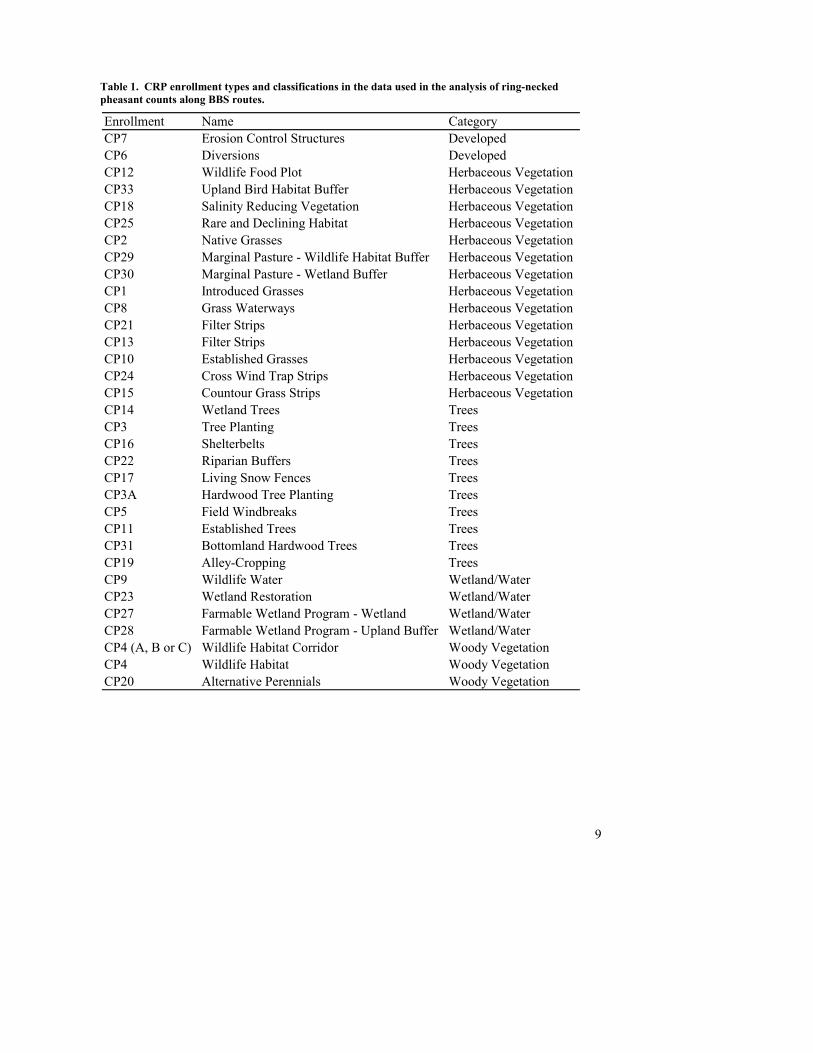
List of Tables Table 1. CRP enrollment types and classifications in the data used in the analysis of ring-necked pheasant counts
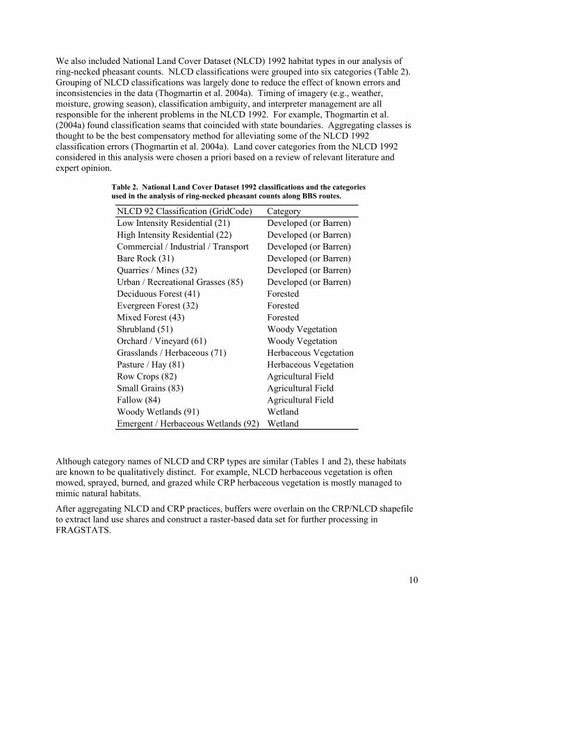
along BBS routes. ................................................................................................................................................9 Table 2. National Land Cover Dataset 1992 classifications and the categories used in the analysis of ring-necked
pheasant counts along BBS routes. ....................................................................................................................10 Table 3. Hectares of CRP enrollment classes in 2004 within the 11 LRRs represented by the 388 analyzed BBS
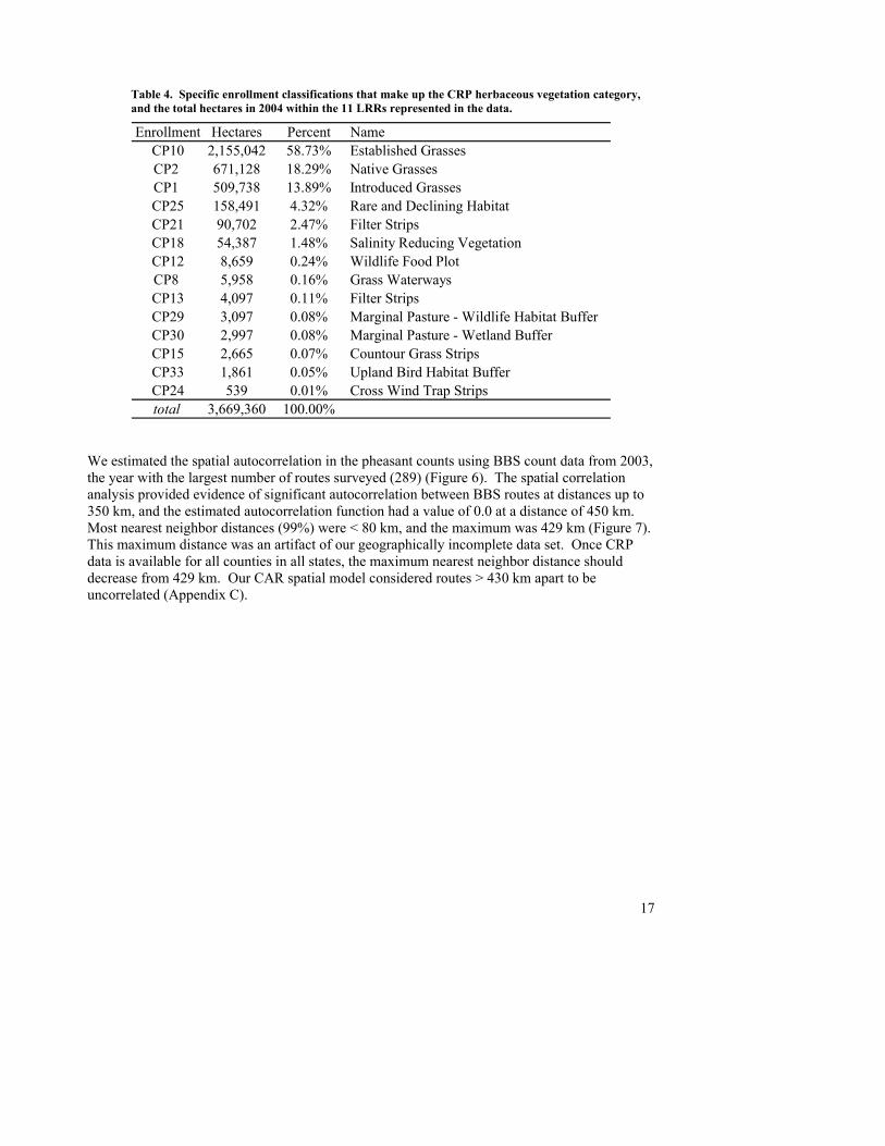
routes used in the analysis, along with the amount found within 1000 m of the survey routes. ........................16 Table 4. Specific enrollment classifications that make up the CRP herbaceous vegetation category, and the total
hectares in 2004 within the 11 LRRs represented in the data. ...........................................................................17 Table 5. Variables in models chosen by DIC backwards elimination for each buffer size.........................................19 Table 6. Means (coefficients) of posterior distributions of standardized model parameters, with 90% credibility
intervals for the entire study area. Distributions were calculated using one chain of length 30,000 after discarding the first 10,000 values.......................................................................................................................20
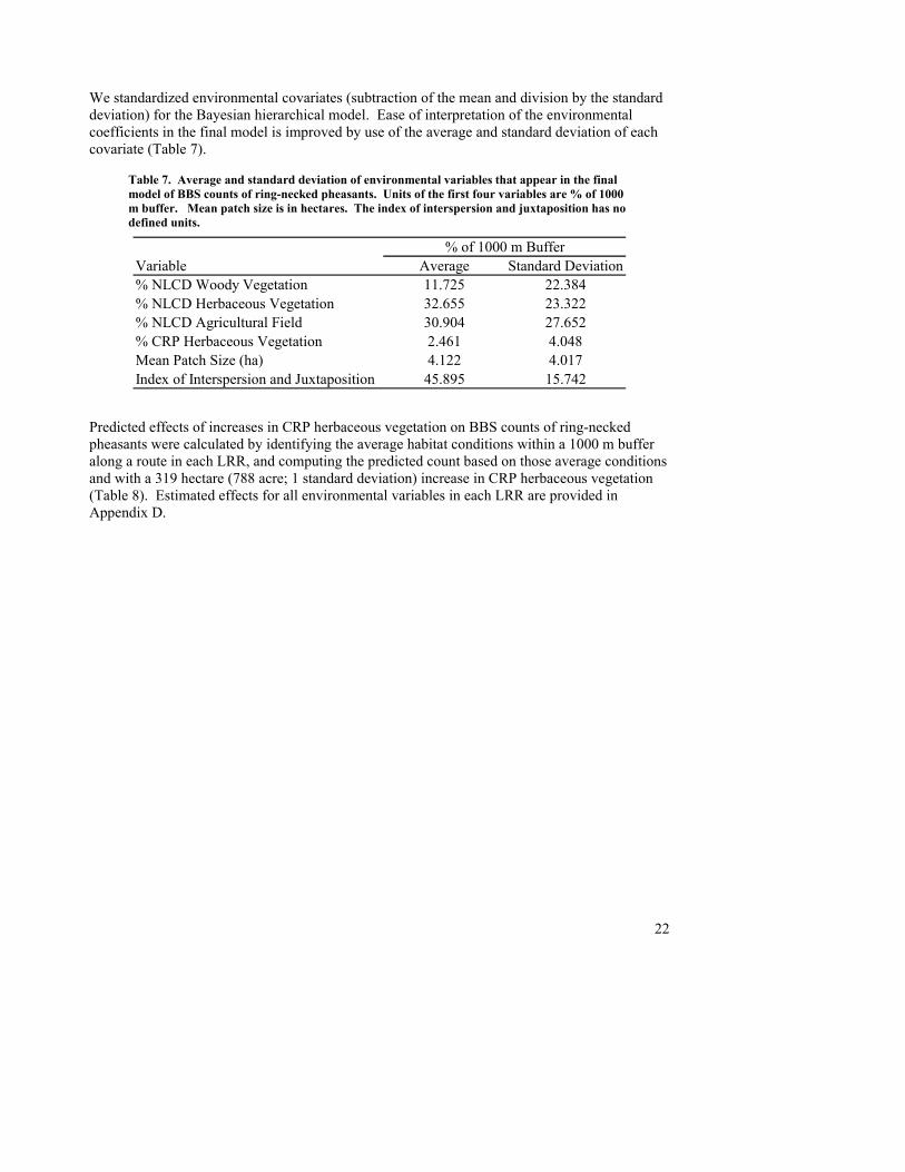
Table 7. Average and standard deviation of environmental variables that appear in the final model of BBS counts of ring-necked pheasants. Units of the first four variables are % of 1000 m buffer. Mean patch size is in hectares. The index of interspersion and juxtaposition has no defined units. ...................................................22
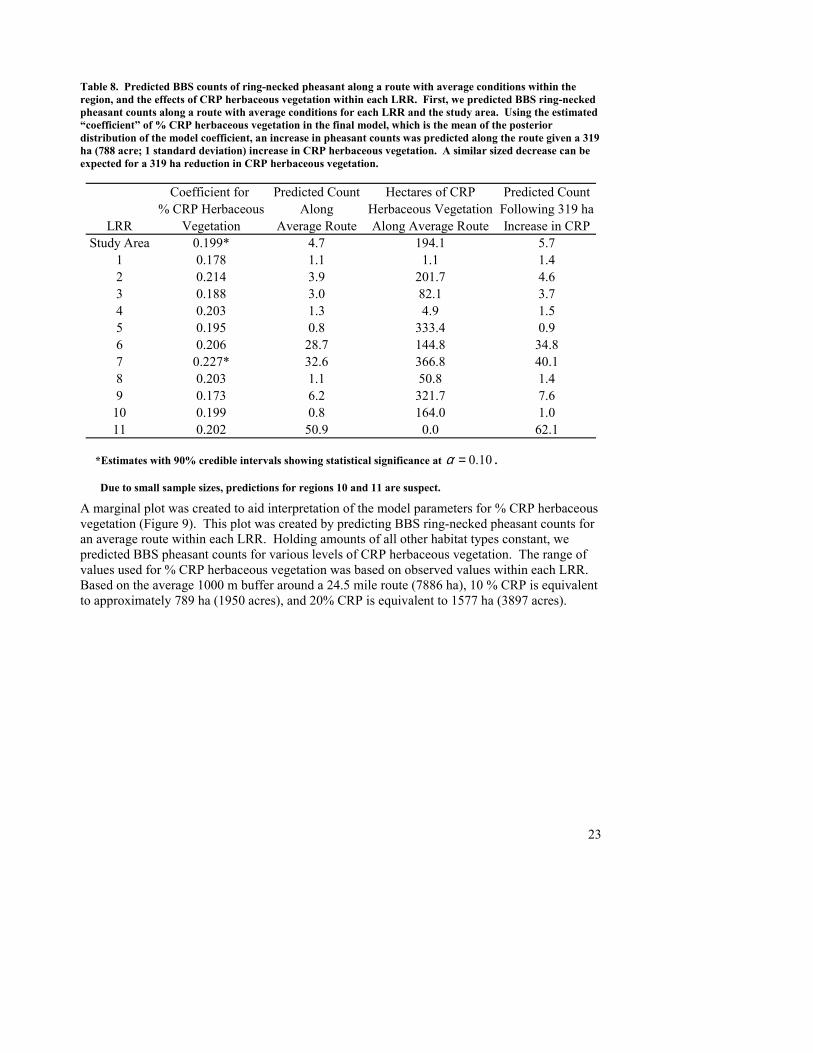
Table 8. Predicted BBS counts of ring-necked pheasant along a route with average conditions within the region, and the effects of CRP herbaceous vegetation within each LRR. First, we predicted BBS ring-necked pheasant counts along a route with average conditions for each LRR and the study area. Using the estimated “coefficient” of % CRP herbaceous vegetation in the final model, which is the mean of the posterior distribution of the model coefficient, an increase in pheasant counts was predicted along the route given a 319 ha (788 acre; 1 standard deviation) increase in CRP herbaceous vegetation. A similar sized decrease can be expected for a 319 ha reduction in CRP herbaceous vegetation. .......................................................................23
Table 9. Coefficients estimated with a fixed effects model in SAS versus the Bayesian hierarchical model estimated using MCMC. ....................................................................................................................................................25
Table 10. Other grassland species and their expected association with CRP fields. Species with a positive association are expected to have increases in breeding populations due to the presence of CRP. Species with negative associations are expected not to benefit or suffer reduced densities because of CRP. ........................29
IV
Table D.1. Estimated coefficients for environmental variables and time trend for each LRR and the entire study area based on posterior distributions of model parameters. Distributions were calculated using one chain of length 30,000 after discarding the first 10,000 values. .................................................................................................52
Table D.2. Estimated random effects for each year based on posterior distributions calculated using one chain of length 30,000 after discarding the first 10,000 values........................................................................................52
Table D.3. Estimated random effects for each BBS route in each LRR using available data based on posterior distributions calculated using one chain of length 30,000 after discarding the first 10,000 values. ..................53
List of Figures Figure 1. Range map for Ring-necked Pheasants. (Taken from Ridgely et al. 2003) .................................................3 Figure 2. Map of Land Resource Regions. ...................................................................................................................4 Figure 3. BBS Routes in the 48 coterminous states......................................................................................................5 Figure 4. LRRs and number of BBS routes in the 9 states contained in data used for evaluating ring-necked
pheasant response to CRP. .................................................................................................................................15 Figure 5. Histogram of counts of Ring-necked Pheasants along 388 BBS routes surveyed during 1987 – 2005.......16 Figure 6. Moran’s I statistics and estimated autocorrelation function for total number of pheasants observed on a
BBS route in 2003. Vertical bars are Bonferroni-corrected 95% confidence intervals on Moran’s I. The darker line is the smoothed autocorrelation function. ........................................................................................18
Figure 7. Histogram and summary statistics of nearest neighbor distances for analyzed BBS routes in our data surveyed in 2003. ...............................................................................................................................................18
Figure 8. Means (coefficients) of posterior distributions of standardized model parameters for each LRR and the entire study area. Distributions were calculated using one chain of length 30,000 after discarding the first 10,000 values. Estimates with 90% credible intervals that included zero are marked with closed circles, ●. Estimates with 90% credible intervals showing statistical significance (did not include zero at the
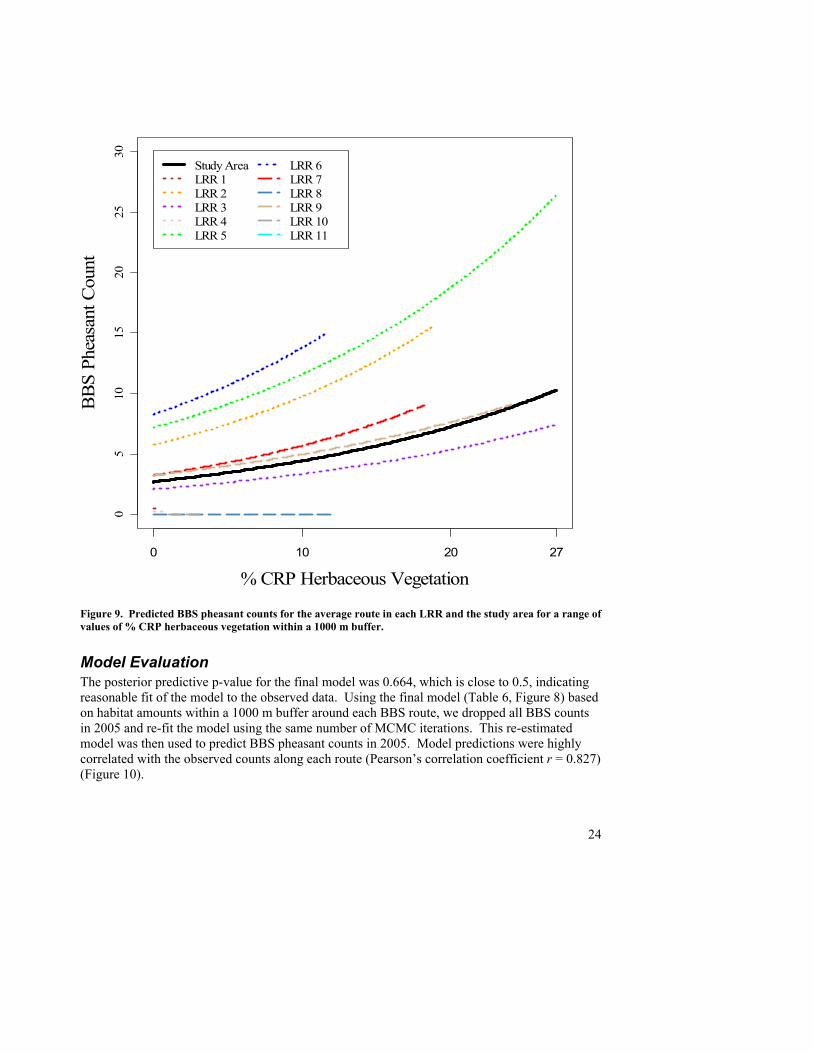
0.10α = level) are marked with asterisks, *. ..................................................................................................21 Figure 9. Predicted BBS pheasant counts for the average route in each LRR and the study area for a range of values
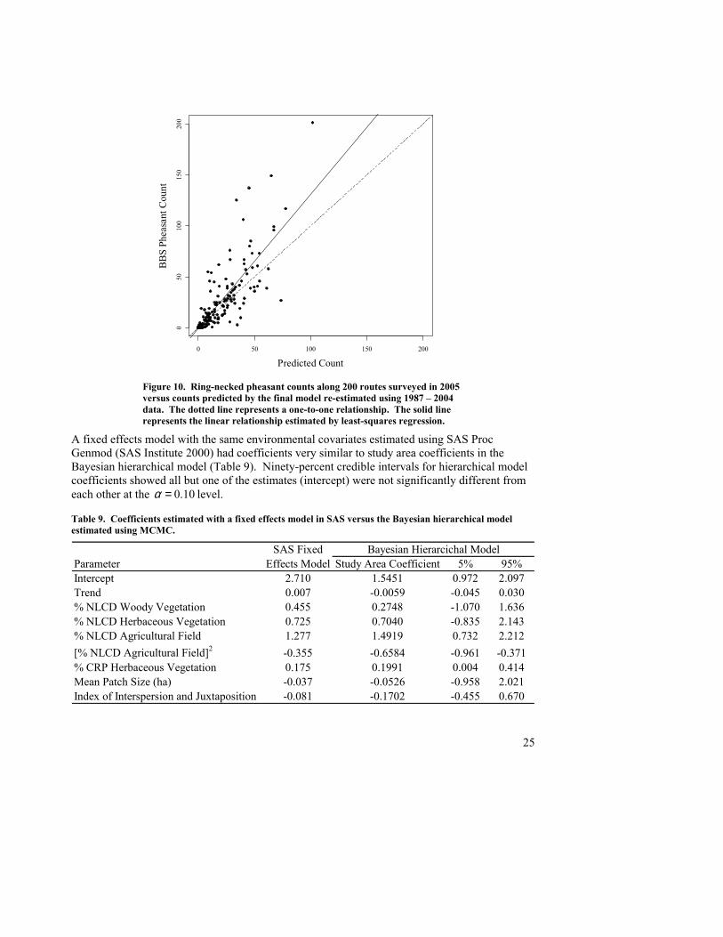
of % CRP herbaceous vegetation within a 1000 m buffer. ................................................................................24 Figure 10. Ring-necked pheasant counts along 200 routes surveyed in 2005 versus counts predicted by the final
model re-estimated using 1987 – 2004 data. The dotted line represents a one-to-one relationship. The solid line represents the linear relationship estimated by least-squares regression.....................................................25
Figure 11. Ring-necked pheasant counts along 200 routes surveyed in 2005 versus counts predicted by a model with % total CRP in place of % CRP herbaceous vegetation. This model was estimated using 1987 – 2004 data. The dotted line represents a one-to-one relationship. The solid line represents the linear relationship estimated by least-squares regression.................................................................................................................................27
Report Citation: Nielson, R. M., L. L. McDonald, J. P. Sullivan, C. Burgess, D. S. Johnson, and S. Howlin. 2006. Estimating response of the ring-necked pheasant (Phasianus colchicus) to the Conservation Reserve Program. Technical report prepared for US Department of Agriculture Farm Service Agency, Contract Number 53-3151-5-8059, Western EcoSystems Technology, Inc., 2003 Central Avenue, Cheyenne, WY 82001.
1
Executive Summary • We evaluated benefits of the Conservation Reserve Program (CRP) to ring-necked
pheasant (Phasianus colchicus) populations by modeling Breeding Bird Survey (BBS) counts of ring-necked pheasants along 388 BBS routes in the US during 1987 – 2005.
• The BBS is conducted yearly, although not every route is surveyed every year. Routes are identified as 24.5-mile sections of secondary road, and counts of various species are based on the total number of birds seen/heard during a three-minute interval at each of fifty stops located at 0.5-mile intervals along the route.
• Predictor variables considered in the statistical analysis included a time trend (percent change per year), percentages of major habitat types (agricultural field, woody and herbaceous vegetation, forested, developed, wetland) identified in the National Land Cover Dataset 1992 within a 1000 m buffer around each route, percentages of CRP enrollment types (woody and herbaceous vegetation, trees, wetland/water) within a 1000 m buffer around each route, along with mean patch size (ha) and an index of interspersion and juxtaposition – a measure of the distribution of patch type adjacencies.
• Computer software (FRAGSTATS) was used to calculate an index of interspersion/juxtaposition of land use categories and edge density, by identifying NLCD and CRP categories as unique patch types. Patches were identified as groups of 30 m by 30 m cells falling into one of the 14 NLCD and CRP categories.
• CRP data available from the following states within the range of ring-necked pheasants in the US were available for analysis: Minnesota, North Dakota, South Dakota, Nebraska, Kansas, Missouri, Utah, Idaho, and Oregon. Only ring-necked pheasant counts along BBS routes within these states were used in the analysis.
• BBS pheasant counts were modeled as over-dispersed Poisson counts in a Bayesian hierarchical model estimated with Markov chain Monte Carlo methods. This method allowed for simultaneous estimation of the effects of environmental variables like CRP and NLCD habitat types within each of 11 Land Resource Regions (LRR) and across the entire study area.
• The Deviance Information Criterion (DIC) was used as a guide to help identify the most parsimonious model to predict ring-necked pheasant counts along BBS routes.
• The study-area wide final model for estimating the number of ring-necked pheasants counted along a BBS route in year i was:
exp[1.5451 0.0059( 1996) 0.2748(NLCD Woody Vegetation)i iT year= − − + +
0.7040(NLCD Herbaceous Vegetation) 1.4949(NLCD Agricultural Field)+ − 20.6584(NLCD Agricultural Field) 0.1991(CRP Herbaceous Vegetation)+ −
0.0526(Mean Patch Size) 0.1702(Interspersion and Juxtaposition)]− .
• Based on this model there is an estimated 1.22 fold, or 22%, increase in ring-necked pheasant counts along a BBS route associated with every increase of 319 ha (788 acres) of CRP herbaceous vegetation within a 1000 m buffer around the route. Three hundred nineteen ha is 4.05 % of an average buffer.
2
• A goodness-of-fit test indicated the final model adequately fit the observed data, and model validation showed predictions from the final model were highly correlated with actual BBS counts (r = 0.827).
• The methodology, analyses and models presented in this report can be performed and repeated periodically to track effects of changes in CRP lands on changes in ring-necked pheasant populations resulting from new enrollments and expiration of existing contracts. These methods can also be extended to other species counted during Breeding Bird Surveys and to other states and LRRs as CRP and NLCD information is updated or becomes available.
Acknowledgements We thank Shawn Bucholtz (USDA, Economic Research Service) for his help in the data collection and processing phases of this project. We also thank Douglas Johnson (USGS, Northern Prairie Wildlife Research Center), Skip Hyberg and Richard Iovanna (USDA, Farm Service Agency) for their ideas and helpful reviews of early versions of this report. John Sauer (USGS, Patuxent Wildlife Research Center) and Wayne Thogmartin (USGS, Upper Midwest Environmental Sciences Center) provided helpful advice during the planning stages of this project. However, the authors of this report are solely responsible for its content.
Introduction To better evaluate benefits to wildlife populations when considering Conservation Reserve Program (CRP) offers and to comply with the Government Performance and Results Act (GPRA), the Farm Service Agency (FSA) needs accurate estimates of the responses of wildlife populations to land use changes and habitat development related to CRP practices throughout the United States (US) and the ability to relate changes in those populations to changes in CRP lands. FSA’s June 2004 CRP Overview (Barbarika et al. 2004), states that “Over 34.7 million acres of environmentally sensitive and fragile lands have been placed into grass and trees that improve the soil, water, air, and wildlife resources of the Nation.”
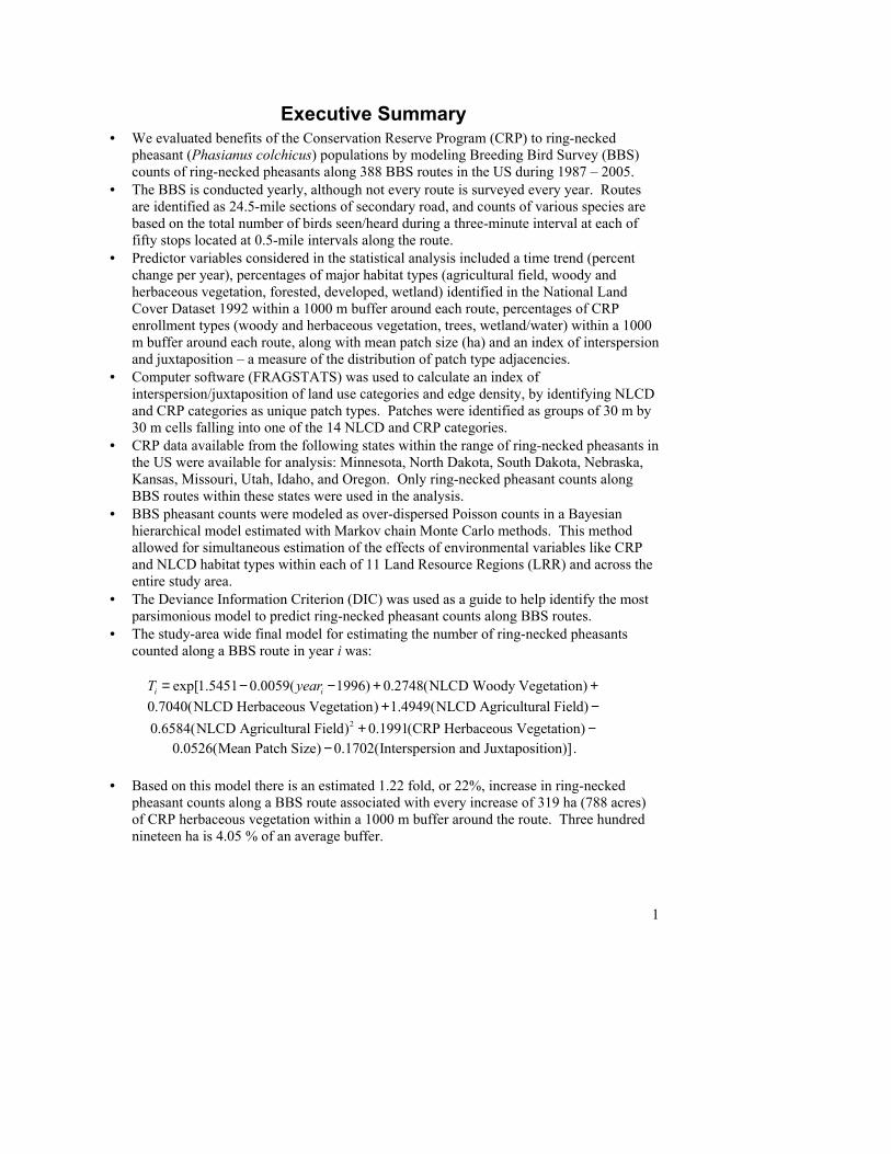
CRP practices not only have strong potential benefit to wildlife, but also reduce soil erosion and improve air and water quality. For example, field windbreaks can reduce wind erosion and improve air quality. Filter strips can improve water quality. These same practices potentially benefit wildlife by providing increased wildlife habitat. Other CRP practices focus directly on benefits to wildlife by planting wildlife food plots, restoring native vegetation and wetlands, etc. Barbarika et al. (2004) list 29 different CRP practices that may benefit wildlife species. The objective of this report is to assess how ring-necked pheasant (Phasianus colchicus) populations in their range within the US (Figure 1) have responded to the set-aside of environmentally sensitive cropland and some pasture.
3
Figure 1. Range map for Ring-necked Pheasants. (Taken from Ridgely et al. 2003)
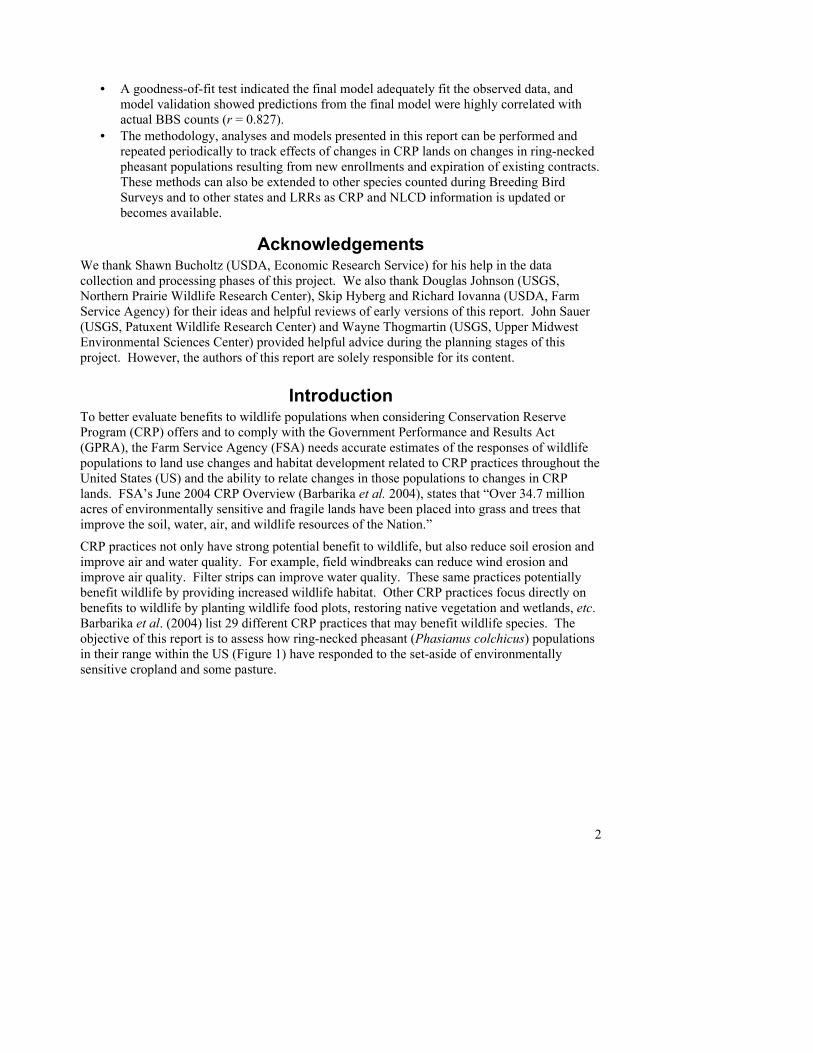
Our goal was to provide a thorough, objective, and scientifically rigorous methodology to: 1) relate indices of ring-necked pheasant populations based on the Breeding Bird Survey (BBS, administered by the United States Geological Survey (USGS); http://www.mbr-pwrc.usgs.gov/bbs/bbs.html) to land use changes and habitat development due to CRP practices, and 2) allow FSA to annually generate updated estimates of the responses. Analyses were performed on Land Resource Regions (LRR) (Figure 2) and aggregated into summary statistics for all states for which data were available. The methodology and models should allow the FSA to expand the methods into states and regions as additional CRP lands and practices are digitized into a GIS, and potentially to other breeding bird species. The methodology, analyses and model selection can be performed and repeated periodically to track effects of changes in CRP lands on changes in ring-necked pheasant population trends, resulting from new enrollments and expiration of existing contracts.
4
Figure 2. Map of Land Resource Regions.
We anticipated that the best indicator variable (metric) available from BBS data to meet FSA objectives was abundance of ring-necked pheasants as indexed by recorded occurrence along a BBS route. This dependent variable would measure the response of pheasants to land use changes and habitat development associated with CRP implementation. The statistical analysis methods (models) for prediction of abundance of pheasants will allow the FSA to generate annual estimates of effects of CRP practices on the selected wildlife species. For a given region, estimates of the relative abundance of pheasants per standard BBS route can be given for a range of hectares (acres) of CRP lands of various practices within 400, 700, or 1000 m of the randomly located BBS routes. In particular, estimates can be given on an annual basis, e.g., for relative abundance of the ring-necked pheasants per standard BBS route with the average hectares of CRP land of various practices within areas surrounding the BBS routes. These annual estimates should allow the FSA to meet the GPRA requirements that programs set measurable goals and measure progress in meeting those goals. Further, results should be useful for communication with decision and policy-makers concerning CRP benefits and refinement of program priorities.
Description of Breeding Bird Survey BBS Program Breeding Bird Surveys are conducted along secondary roads during the peak of the nesting season, primarily in June, although surveys in desert regions and some southern states (where the
5
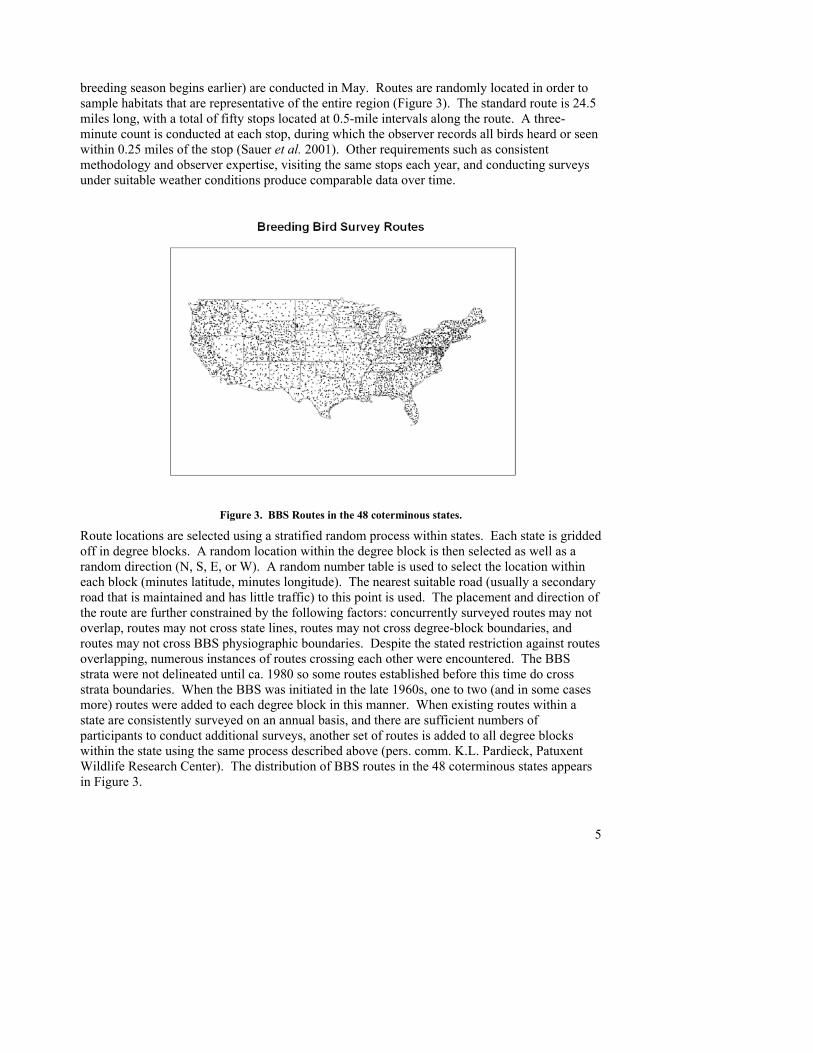
breeding season begins earlier) are conducted in May. Routes are randomly located in order to sample habitats that are representative of the entire region (Figure 3). The standard route is 24.5 miles long, with a total of fifty stops located at 0.5-mile intervals along the route. A three-minute count is conducted at each stop, during which the observer records all birds heard or seen within 0.25 miles of the stop (Sauer et al. 2001). Other requirements such as consistent methodology and observer expertise, visiting the same stops each year, and conducting surveys under suitable weather conditions produce comparable data over time.
Figure 3. BBS Routes in the 48 coterminous states.
Route locations are selected using a stratified random process within states. Each state is gridded off in degree blocks. A random location within the degree block is then selected as well as a random direction (N, S, E, or W). A random number table is used to select the location within each block (minutes latitude, minutes longitude). The nearest suitable road (usually a secondary road that is maintained and has little traffic) to this point is used. The placement and direction of the route are further constrained by the following factors: concurrently surveyed routes may not overlap, routes may not cross state lines, routes may not cross degree-block boundaries, and routes may not cross BBS physiographic boundaries. Despite the stated restriction against routes overlapping, numerous instances of routes crossing each other were encountered. The BBS strata were not delineated until ca. 1980 so some routes established before this time do cross strata boundaries. When the BBS was initiated in the late 1960s, one to two (and in some cases more) routes were added to each degree block in this manner. When existing routes within a state are consistently surveyed on an annual basis, and there are sufficient numbers of participants to conduct additional surveys, another set of routes is added to all degree blocks within the state using the same process described above (pers. comm. K.L. Pardieck, Patuxent Wildlife Research Center). The distribution of BBS routes in the 48 coterminous states appears in Figure 3.
6
The BBS produces an index of relative abundance rather than a complete count or density of breeding bird populations. Data analyses of BBS counts assume that fluctuations in these indices of abundance are representative of the population as a whole (Sauer et al. 2001).
Bystrak (1981) discusses the utility of the BBS and states that it has demonstrated its usefulness as an effective index of bird population levels, both temporally and spatially. However, he states that species susceptible to harsh winters may show large annual fluctuations. The BBS is also biased toward those species detectable from roadsides. When habitats along roads change at a different rate than those in the region, the trends identified by the BBS might not be representative of the region as a whole (Bart et al. 1995).
The ability of the BBS to detect population changes will vary by species. Since BBS routes are along roads, the BBS will be better able to detect change in those species likely to be observed along roads. Hanowski and Niemi (1995) suggest that if the major habitat type off-road is distinctly different from that found along roads, the sensitivity of road surveys might be lower than off-road surveys. Conversely, if the habitat away from roads is similar to that along the sampling route, road surveys would likely be representative of the surrounding areas. In an agricultural region where the fields extend practically to the road edge, the BBS may do a very good job of counting most of the species in the area. The BBS also is good at identifying trends associated with broad regional changes, such as acid rain (Hames et al. 2002). The BBS is most likely to be sensitive to population changes of those species likely to be observed along roads where the roadside habitat is representative of the larger area, and the factors affecting the bird population are present along the road. For more details of the BBS program, see http://www.pwrc.usgs.gov/BBS/.
Data Collection Methods A detailed, step-by-step description of all methods and sources of data can be found in Appendix A.
BBS Data GIS data for North American BBS digitized routes were available from the Bird Conservation Node of the National Biological Information Infrastructure (http://mbirdims.fws.gov/nbii/). Bird count data are available from the U.S. Geological Survey’s Patuxent Wildlife Research Center’s website (http://www.pwrc.usgs.gov). Each BBS route has a unique identifier consisting of a two digit state code and a three digit route code.
Data Processing Since no records were present in the BBS data to indicate years when the route was surveyed but no individuals of a species were observed, these records of zero ring-necked pheasant counts had to be created. Care was taken to ensure that counts of zero ring-necked pheasants were only created for years a route was actually surveyed, since many routes are not surveyed every year. Additional variables considered for use in the analyses were available from the Weather and Route files. Finally, only records pertaining to ring-necked pheasants were retained for analysis.
Formatted: Font color: Auto
7
GIS Methods To evaluate the relative abundance of pheasants in the vicinity of CRP lands associated with BBS routes, routes were buffered at three levels – extending radially outward from the route at distances of 400 m, 700 m, and 1000 m. If BBS routes were straight lines, these buffer sizes would correspond to 7794 acres, 13,640 acres, 19,487 acres, respectively. Buffer areas around nearby routes were maintained separately so that the area around each route could be evaluated individually. These three buffer sizes were chosen based on the BBS survey protocol (i.e., birds are counted if seen or heard within ¼ mile ~ 400 meters), potential home range sizes, and daily movements (Giudice and Ratti 2001).
There were three instances where one BBS route was replaced by another during the time period considered by this study. For example, route 81114 contained much of the same survey area as route 81014. Route 81014 was run intermittently through 1999, and route 81114 has been surveyed since 2000. To preserve independence between the BBS routes, we combined the survey data for these pairs of routes (81014 and 81114; 33024 and 33124; 50040 and 50140) and considered the pair to be one route for the analysis.
Conservation Reserve Program GIS Data CRP data were provided by the FSA, and processed by the USDA Economic Research Service (ERS). As of November, 2005, data for nine states in the range of pheasants were available for analysis: Idaho; Kansas; Minnesota; Missouri; Nebraska; North Dakota; Oregon; South Dakota; and Utah. CRP GIS data were available in two different formats. The older format included Common Land Unit (CLU) shapefiles and associated CRP tables for each county. The CLU shapefiles contained boundaries for all farm fields. The CRP tables contained contract identifier and practice information. Data for Idaho, North Dakota, South Dakota, and most counties in Missouri were received in this format. An updated version was received for Kansas, Nebraska, Minnesota, Oregon, and Utah. This version included CRP shapefiles for each county. The CRP shapefiles contained boundaries for only the CRP fields. The CRP shapefiles contained some contract and practice information. There were 20 BBS routes partially or fully within a few counties of Missouri with incomplete CRP data, and these routes were dropped from the analysis. In many instances, the available CRP data did contain information that would allow estimation of the age of a contract. However, a major limitation was that the current snapshot of CLU did not contain parcels with expired CRP contracts. Therefore, it was not possible to develop a snapshot of CRP for any time period prior to the first release of the CLU data (2004), and therefore, it was not possible to develop a longitudinal dataset of CRP. This imposed a limitation on the data analysis, as the preferred analysis would take a longitudinal approach to modeling CRP practice types, amounts, and age (e.g., CRP enrollments along a route would mature through time).
Processing Conservation Reserve Program GIS Data All county-level ArcView shapefiles were combined into a single state-wide file. Prior to combining into state-wide files, some data clean-up was required to ensure all files were in the same GIS format, and all attributes possessed standardized names for all counties. The older version of the CRP data required more processing prior to use. Since the files contained boundaries for all farm fields, those fields enrolled in the CRP program first had to be extracted.
8
Then the CRP practice data needed to be associated with those parcels. Some records in tables containing the CRP parcel specific data were missing information, particularly for CRP cover practices.
To fill in missing information, we used the Fiscal Year 2002 and a monthly upload of June 2004 data from the national CRP contracts database. This national database contained all the information for each CRP contract. The output was a state-wide CRP shapefile with all the attributes necessary for the subsequent modeling procedures.
It was possible for a contract to have multiple practices and for there to be no further information on how those practices were distributed within the parcels. A solution was created so that when a buffer edge intersected CRP contract parcels, we could assign proportions of the areas of specific CRP practices to be within the buffer. In some instances, the number of acres for a practice and the size of a parcel matched. In that case, we assumed that practice was restricted to a single parcel for that contract.
In other instances, a single parcel contained multiple CRP practices. In those instances, two approaches were necessary. To most accurately assign the proportion of area for a specific CRP practice within the buffer, the different practices were randomly spread across the parcel(s) of the contract based on known shares. While this method was useful for achieving correct proportions, it would have artificially inflated the amount of edge and number of patches within the parcels, thereby biasing estimates of edge density and interspersion and juxtaposition as measured by FRAGSTATS (see below). Therefore, in the second approach each parcel was assigned the dominant practice for the contract.
Once a usable CRP shapefile with attached cover group data was created, we combined CRP practices into 5 categories (Table 1). This was necessary due to the small acreage of specific CRP enrollment types across the landscape. In addition, it is believed the effect of CRP enrollment types and ages on pheasant abundance is largely due to differences in vegetation structure (Eggebo et al. 2003), so our 5 CRP categories represent different vegetation structures.
9
Table 1. CRP enrollment types and classifications in the data used in the analysis of ring-necked pheasant counts along BBS routes.
Enrollment Name CategoryCP7 Erosion Control Structures DevelopedCP6 Diversions DevelopedCP12 Wildlife Food Plot Herbaceous VegetationCP33 Upland Bird Habitat Buffer Herbaceous VegetationCP18 Salinity Reducing Vegetation Herbaceous VegetationCP25 Rare and Declining Habitat Herbaceous VegetationCP2 Native Grasses Herbaceous VegetationCP29 Marginal Pasture - Wildlife Habitat Buffer Herbaceous VegetationCP30 Marginal Pasture - Wetland Buffer Herbaceous VegetationCP1 Introduced Grasses Herbaceous VegetationCP8 Grass Waterways Herbaceous VegetationCP21 Filter Strips Herbaceous VegetationCP13 Filter Strips Herbaceous VegetationCP10 Established Grasses Herbaceous VegetationCP24 Cross Wind Trap Strips Herbaceous VegetationCP15 Countour Grass Strips Herbaceous VegetationCP14 Wetland Trees TreesCP3 Tree Planting TreesCP16 Shelterbelts TreesCP22 Riparian Buffers TreesCP17 Living Snow Fences TreesCP3A Hardwood Tree Planting TreesCP5 Field Windbreaks TreesCP11 Established Trees TreesCP31 Bottomland Hardwood Trees TreesCP19 Alley-Cropping TreesCP9 Wildlife Water Wetland/WaterCP23 Wetland Restoration Wetland/WaterCP27 Farmable Wetland Program - Wetland Wetland/WaterCP28 Farmable Wetland Program - Upland Buffer Wetland/WaterCP4 (A, B or C) Wildlife Habitat Corridor Woody VegetationCP4 Wildlife Habitat Woody VegetationCP20 Alternative Perennials Woody Vegetation
10
We also included National Land Cover Dataset (NLCD) 1992 habitat types in our analysis of ring-necked pheasant counts. NLCD classifications were grouped into six categories (Table 2). Grouping of NLCD classifications was largely done to reduce the effect of known errors and inconsistencies in the data (Thogmartin et al. 2004a). Timing of imagery (e.g., weather, moisture, growing season), classification ambiguity, and interpreter management are all responsible for the inherent problems in the NLCD 1992. For example, Thogmartin et al. (2004a) found classification seams that coincided with state boundaries. Aggregating classes is thought to be the best compensatory method for alleviating some of the NLCD 1992 classification errors (Thogmartin et al. 2004a). Land cover categories from the NLCD 1992 considered in this analysis were chosen a priori based on a review of relevant literature and expert opinion.
Table 2. National Land Cover Dataset 1992 classifications and the categories used in the analysis of ring-necked pheasant counts along BBS routes.
NLCD 92 Classification (GridCode) CategoryLow Intensity Residential (21) Developed (or Barren)High Intensity Residential (22) Developed (or Barren)Commercial / Industrial / Transport Developed (or Barren)Bare Rock (31) Developed (or Barren)Quarries / Mines (32) Developed (or Barren)Urban / Recreational Grasses (85) Developed (or Barren)Deciduous Forest (41) ForestedEvergreen Forest (32) ForestedMixed Forest (43) ForestedShrubland (51) Woody VegetationOrchard / Vineyard (61) Woody VegetationGrasslands / Herbaceous (71) Herbaceous VegetationPasture / Hay (81) Herbaceous VegetationRow Crops (82) Agricultural FieldSmall Grains (83) Agricultural FieldFallow (84) Agricultural FieldWoody Wetlands (91) WetlandEmergent / Herbaceous Wetlands (92) Wetland
Although category names of NLCD and CRP types are similar (Tables 1 and 2), these habitats are known to be qualitatively distinct. For example, NLCD herbaceous vegetation is often mowed, sprayed, burned, and grazed while CRP herbaceous vegetation is mostly managed to mimic natural habitats.
After aggregating NLCD and CRP practices, buffers were overlain on the CRP/NLCD shapefile to extract land use shares and construct a raster-based data set for further processing in FRAGSTATS.
11
Several landscape indices were identified that could be calculated using FRAGSTATS. FRAGSTATS is a stand-alone program that can accept ArcInfo GRID output as input for processing. The FRAGSTATS program and detailed description of its use can be obtained, free of charge, at http://www.umass.edu/landeco/research/fragstats/fragstats.html. FRAGSTATS was used to calculate an index of interspersion/juxtaposition (McGarigal and Marks 1985) of land use categories and edge density, by identifying NLCD and CRP categories as unique patch types. Patches were identified as groups of 30 m by 30 m cells falling into one of the 14 NLCD and CRP categories.
QA/QC of GIS Output To verify and validate the GIS methods employed, we developed a set of steps intended for quality assurance / quality control. In addition to data on the amount of CRP land contained within a buffer region surrounding a BBS route, data were also provided on the amount of the various NLCD coverage groupings (Table 2) within this same area. In particular, because the underlying CRP data are confidential, these data were utilized for quality control purposes.
To generate the dataset to perform quality control, we first downloaded the NLCD raster dataset for each of the nine states from http://www.seamless.usgs.gov/. The state-wide raster was cut down to the shape of the BBS route buffers utilizing the ArcGIS Extract Clip function, working one route buffer at a time. The resulting polygons were then spatially joined to the buffers to acquire the appropriate attributes, and the files were converted to ASCII format to be run in the FRAGSTATS application in batch mode. The final output consisted of the amount of land within the buffer falling within each of the NLCD groupings and the results of the FRAGSTATS analysis which computed the amount of edge density within each buffer and an index of interspersion and juxtaposition. These data were collated with the output from the USDA-ERS analysis and compiled into a table for further evaluation.
Assigning BBS Routes to USDA Land Resource Regions We assigned each BBS route to a LRR (Figure 2). The LRR information was downloaded as an ArcInfo coverage from http://www.nrcs.usda.gov/technical/land/aboutmaps/us48mlra.html. The BBS routes from each state were overlain onto the map of the LRRs. To assign routes to LRRs, the shapefile containing the BBS routes was “intersected” with the shapefile containing the LRRs. For routes crossing LRR boundaries, each route was assigned to the LRR that contained the most length.
12
Statistical Analysis and Modeling Methods
Bayesian Hierarchical Model The status and trends in ring-necked pheasant population numbers likely have high variation across routes, and CRP practices are likely different across larger regions. To accommodate this complex structure of spatial heterogeneity, we took a Bayesian hierarchical modeling approach to this analysis similar to the methodology described in Thogmartin et al. (2006) and Thogmartin et al. (2004b). A Bayesian hierarchical model was fit using Markov chain Monte Carlo (MCMC) methods (Link et al. 2002) to model BBS counts of ring-necked pheasants as overdispersed Poisson counts (i.e., the variance is larger than the standard Poisson distribution). This model viewed BBS counts as resulting from a multilevel probability structure. At the highest level (i.e., study area), it is believed that BBS counts are related to a set of hyper-parameters, which govern the overall relationship of counts with environmental and longitudinal covariates. However, regional differences in these relationships are believed to exist and parameters at the regional scale are viewed as random variables. Many researchers feel these complex models are necessary for successfully modeling the heterogeneity in BBS counts and designing management plans. For examples, see Link et al. (2002), Link and Sauer (2002), Sauer and Link (2002), and Thogmartin et al. (2004b; 2006).
Trends in BBS pheasant counts and relationships with land cover types and CRP practices were estimated for each LRR, as well as for the study area as a whole. Using counts of ring-necked pheasants since the beginning of the CRP (1987 through 2005) along routes where at least one ring-necked pheasant had been observed during this period, we modeled the expected value
ijtλ of count ijtY in LRR i, at route j, in year t as
*
1
log[ ] ( )p
ijt i i ik ijk t ij ijtk
LRR t t xλ γ β α ω ε=
= + − + + + +∑ , [1]
where *t is the median year (1996) from which change is measured, iγ is the trend over time (change per year) in LRR i, ikβ are environmental (fixed) effects of covariates ijkx in LRR i, k indexes the number of environmental effects, tα are random year effects, ijω are random route-specific effects, and ijtε are overdispersion Poisson errors. Year 1987 was chosen as the first year for data in the analysis because CRP enrollments began in 1986.
Environmental covariates representing amounts of land cover (NLCD or CRP types), as well as patch metrics (e.g., average patch size and interspersion and juxtaposition) were treated as fixed effects. We standardized each environmental covariate to increase the efficiency of the MCMC process (Gilks and Roberts 1996). Standardization involved subtracting the mean value and dividing by the standard deviation. The model was fit using WinBUGS 1.4.1 (Speigelhalter et al. 2003a), which can be obtained free of charge at http://www.mrc-bsu.cam.ac.uk/bugs/. The code for estimating parameters of this model is in Appendix B, the data and initial values files are archived at WEST, Inc., and will be provided to FSA on a CD to accompany this report.
There are two key differences between our model (1) and the models used by Thogmartin et al. (2004b; 2006). The first is that we did not include a term for observer differences (biases), as
13
ring-necked pheasants are easily detectable and identifiable (Gough et al. 1998). Observer differences are believed to be an important component in models of BBS counts of rare and elusive species (Link and Sauer 1994). However, ring-necked pheasants, although declining in some areas, are not rare. Investigation into potential observer differences found no evidence of such effects for northern bobwhite (Colinus virginianus) (pers. comm. W. Thogmartin, USGS), another bird in the family.
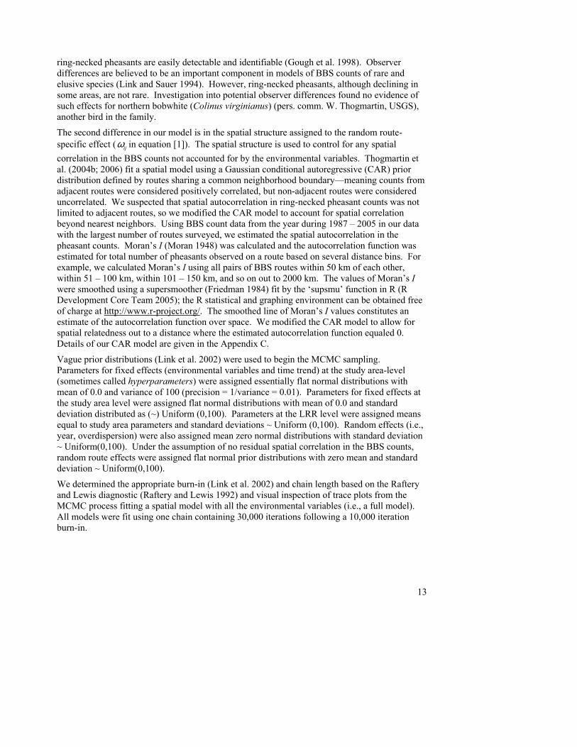
The second difference in our model is in the spatial structure assigned to the random route-specific effect ( ijω in equation [1]). The spatial structure is used to control for any spatial correlation in the BBS counts not accounted for by the environmental variables. Thogmartin et al. (2004b; 2006) fit a spatial model using a Gaussian conditional autoregressive (CAR) prior distribution defined by routes sharing a common neighborhood boundary—meaning counts from adjacent routes were considered positively correlated, but non-adjacent routes were considered uncorrelated. We suspected that spatial autocorrelation in ring-necked pheasant counts was not limited to adjacent routes, so we modified the CAR model to account for spatial correlation beyond nearest neighbors. Using BBS count data from the year during 1987 – 2005 in our data with the largest number of routes surveyed, we estimated the spatial autocorrelation in the pheasant counts. Moran’s I (Moran 1948) was calculated and the autocorrelation function was estimated for total number of pheasants observed on a route based on several distance bins. For example, we calculated Moran’s I using all pairs of BBS routes within 50 km of each other, within 51 – 100 km, within 101 – 150 km, and so on out to 2000 km. The values of Moran’s I were smoothed using a supersmoother (Friedman 1984) fit by the ‘supsmu’ function in R (R Development Core Team 2005); the R statistical and graphing environment can be obtained free of charge at http://www.r-project.org/. The smoothed line of Moran’s I values constitutes an estimate of the autocorrelation function over space. We modified the CAR model to allow for spatial relatedness out to a distance where the estimated autocorrelation function equaled 0. Details of our CAR model are given in the Appendix C.
Vague prior distributions (Link et al. 2002) were used to begin the MCMC sampling. Parameters for fixed effects (environmental variables and time trend) at the study area-level (sometimes called hyperparameters) were assigned essentially flat normal distributions with mean of 0.0 and variance of 100 (precision = 1/variance = 0.01). Parameters for fixed effects at the study area level were assigned flat normal distributions with mean of 0.0 and standard deviation distributed as (~) Uniform (0,100). Parameters at the LRR level were assigned means equal to study area parameters and standard deviations ~ Uniform (0,100). Random effects (i.e., year, overdispersion) were also assigned mean zero normal distributions with standard deviation ~ Uniform(0,100). Under the assumption of no residual spatial correlation in the BBS counts, random route effects were assigned flat normal prior distributions with zero mean and standard deviation ~ Uniform(0,100).
We determined the appropriate burn-in (Link et al. 2002) and chain length based on the Raftery and Lewis diagnostic (Raftery and Lewis 1992) and visual inspection of trace plots from the MCMC process fitting a spatial model with all the environmental variables (i.e., a full model). All models were fit using one chain containing 30,000 iterations following a 10,000 iteration burn-in.
14
Model Selection During model selection, we considered the effects of covariates listed in Tables 1 and 2, provided these habitats were more than 5% of total area in buffers around BBS routes. We also considered the average patch size within a buffer, and an index of interspersion and juxtaposition. Edge density was found to be negatively correlated with average patch size (Pearson’s correlation coefficients > -0.63 for all buffer sizes) and thus was dropped from the analysis.
The main objective of the analysis was to identify the most parsimonious model, and we used the Deviance Information Criterion (DIC) (Speigelhalter et al. 2003b) as a guide to that end. DIC is a measure of goodness of fit and model complexity – essentially the Bayesian equivalent of Akaike’s Information Criterion (AIC) (Burnham and Anderson 2002). A good model corresponds to a lower DIC. Final models were obtained by backwards variable removal from the full model using the DIC (Speigelhalter et al. 2003b, Thogmartin et al. 2004b). The full model contained a time trend, random year and route effects, the environmental variables listed above, along with quadratic forms for the percent of NLCD agricultural field and percent CRP wetland. At each step of the backwards removal process, each variable was dropped from the model and the resulting DIC was calculated. The variable dropped resulting in the lowest DIC was removed from the previous model, provided the DIC for the resulting model was smaller than the DIC for the previous model. Model selection was performed for each of the three buffer sizes.
Following model selection, the need for the CAR spatial structure was evaluated using the DIC criterion. Provided the final model has the appropriate structure (i.e., overdispersed Poisson), the CAR spatial structure might not be needed if the spatial correlation is accounted for by the model covariates (both nuisance and fixed effects) (Thogmartin et al. 2004b). If the DIC was lowered then the CAR component was included, otherwise, random route effects were assumed to be independent. The resulting model was used to obtain estimates of coefficients and 90% credible intervals for coefficients.
Model Evaluation We measured model goodness-of-fit by the posterior predictive p-value (Gelman and Meng 1996). A p-value close to 0.0 or 1.0 indicates the data do not agree with the proposed model, while a value near 0.5 indicates the model adequately fits the data. We compared model predictions, based on pre-2005 data, to the actual BBS counts in 2005 for all routes in our data. Pearson’s correlation coefficient (Neter et al. 1996) was used to assess the agreement between the model and observed counts. For this evaluation, we dropped all 2005 BBS counts and re-fit the final model using data from 1987 – 2004. The coefficients from this model were then used to predict BBS counts in 2005. We assumed using 2005 for this comparison would provide the most precise evaluation of the final model because the CRP information in the data represented enrollment in 2004.
The models fit using MCMC were compared to similar non-Bayesian models, i.e., overdispersed Poisson models containing only environmental covariates. These simpler models were estimated using Proc GENMOD (SAS Institute 2000). Such comparisons with other data have been used to evaluate support for the objective Bayesian models fit using MCMC (e.g., Thogmartin et al. 2004b).
15
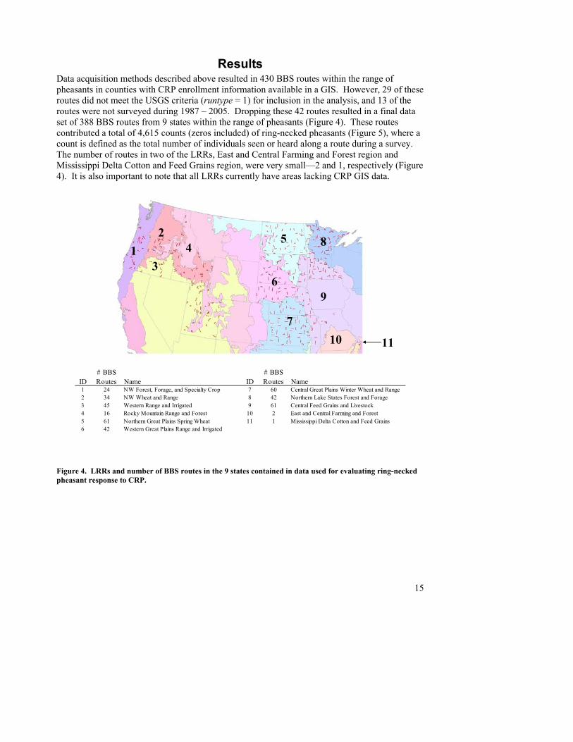
Results Data acquisition methods described above resulted in 430 BBS routes within the range of pheasants in counties with CRP enrollment information available in a GIS. However, 29 of these routes did not meet the USGS criteria (runtype = 1) for inclusion in the analysis, and 13 of the routes were not surveyed during 1987 – 2005. Dropping these 42 routes resulted in a final data set of 388 BBS routes from 9 states within the range of pheasants (Figure 4). These routes contributed a total of 4,615 counts (zeros included) of ring-necked pheasants (Figure 5), where a count is defined as the total number of individuals seen or heard along a route during a survey. The number of routes in two of the LRRs, East and Central Farming and Forest region and Mississippi Delta Cotton and Feed Grains region, were very small—2 and 1, respectively (Figure 4). It is also important to note that all LRRs currently have areas lacking CRP GIS data.
13
24
6
5 8
9
107
11
# BBS # BBSID Routes Name ID Routes Name1 24 NW Forest, Forage, and Specialty Crop 7 60 Central Great Plains Winter Wheat and Range2 34 NW Wheat and Range 8 42 Northern Lake States Forest and Forage3 45 Western Range and Irrigated 9 61 Central Feed Grains and Livestock4 16 Rocky Mountain Range and Forest 10 2 East and Central Farming and Forest5 61 Northern Great Plains Spring Wheat 11 1 Mississippi Delta Cotton and Feed Grains6 42 Western Great Plains Range and Irrigated
Figure 4. LRRs and number of BBS routes in the 9 states contained in data used for evaluating ring-necked pheasant response to CRP.
16
BBS Pheasant Count
Freq
uenc
y
0 50 100 150 200 250 300
050
010
0015
0020
0025
00
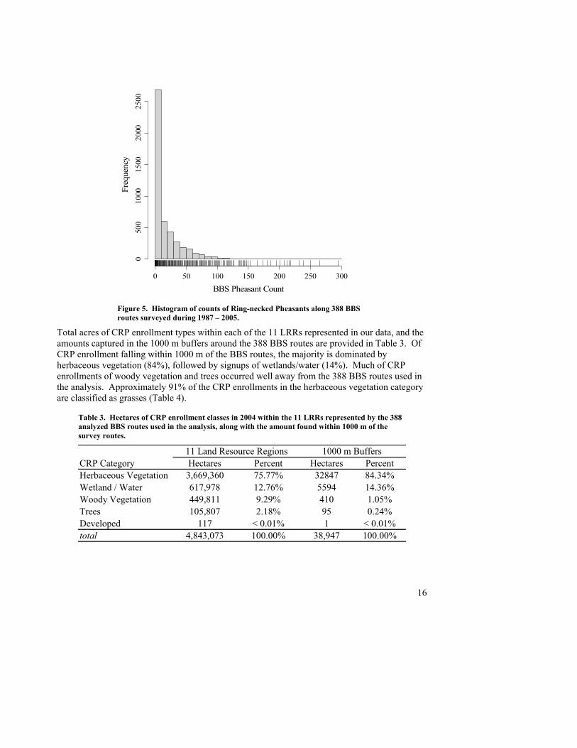
Figure 5. Histogram of counts of Ring-necked Pheasants along 388 BBS routes surveyed during 1987 – 2005.
Total acres of CRP enrollment types within each of the 11 LRRs represented in our data, and the amounts captured in the 1000 m buffers around the 388 BBS routes are provided in Table 3. Of CRP enrollment falling within 1000 m of the BBS routes, the majority is dominated by herbaceous vegetation (84%), followed by signups of wetlands/water (14%). Much of CRP enrollments of woody vegetation and trees occurred well away from the 388 BBS routes used in the analysis. Approximately 91% of the CRP enrollments in the herbaceous vegetation category are classified as grasses (Table 4).
Table 3. Hectares of CRP enrollment classes in 2004 within the 11 LRRs represented by the 388 analyzed BBS routes used in the analysis, along with the amount found within 1000 m of the survey routes.
CRP Category Hectares Percent Hectares PercentHerbaceous Vegetation 3,669,360 75.77% 32847 84.34%Wetland / Water 617,978 12.76% 5594 14.36%Woody Vegetation 449,811 9.29% 410 1.05%Trees 105,807 2.18% 95 0.24%Developed 117 < 0.01% 1 < 0.01%total 4,843,073 100.00% 38,947 100.00%
11 Land Resource Regions 1000 m Buffers
17
Table 4. Specific enrollment classifications that make up the CRP herbaceous vegetation category, and the total hectares in 2004 within the 11 LRRs represented in the data.
Enrollment Hectares Percent NameCP10 2,155,042 58.73% Established GrassesCP2 671,128 18.29% Native GrassesCP1 509,738 13.89% Introduced GrassesCP25 158,491 4.32% Rare and Declining HabitatCP21 90,702 2.47% Filter StripsCP18 54,387 1.48% Salinity Reducing VegetationCP12 8,659 0.24% Wildlife Food PlotCP8 5,958 0.16% Grass WaterwaysCP13 4,097 0.11% Filter StripsCP29 3,097 0.08% Marginal Pasture - Wildlife Habitat BufferCP30 2,997 0.08% Marginal Pasture - Wetland BufferCP15 2,665 0.07% Countour Grass StripsCP33 1,861 0.05% Upland Bird Habitat BufferCP24 539 0.01% Cross Wind Trap Stripstotal 3,669,360 100.00%
We estimated the spatial autocorrelation in the pheasant counts using BBS count data from 2003, the year with the largest number of routes surveyed (289) (Figure 6). The spatial correlation analysis provided evidence of significant autocorrelation between BBS routes at distances up to 350 km, and the estimated autocorrelation function had a value of 0.0 at a distance of 450 km. Most nearest neighbor distances (99%) were < 80 km, and the maximum was 429 km (Figure 7). This maximum distance was an artifact of our geographically incomplete data set. Once CRP data is available for all counties in all states, the maximum nearest neighbor distance should decrease from 429 km. Our CAR spatial model considered routes > 430 km apart to be uncorrelated (Appendix C).

18
0 500 1000 1500 2000
-0.5
0.0
0.5
1.0
Kilometers between BBS Routes
Cor
rela
tion
Figure 6. Moran’s I statistics and estimated autocorrelation function for total number of pheasants observed on a BBS route in 2003. Vertical bars are Bonferroni-corrected 95% confidence intervals on Moran’s I. The darker line is the smoothed autocorrelation function.
0 100 200 300 400
0.00
00.
005
0.01
00.
015
0.02
0
Distance (km)
Den
sity
Mean = 38.26 km
Median = 35.44 km
Stdev = 27.21 km
Figure 7. Histogram and summary statistics of nearest neighbor distances for analyzed BBS routes in our data surveyed in 2003.
19
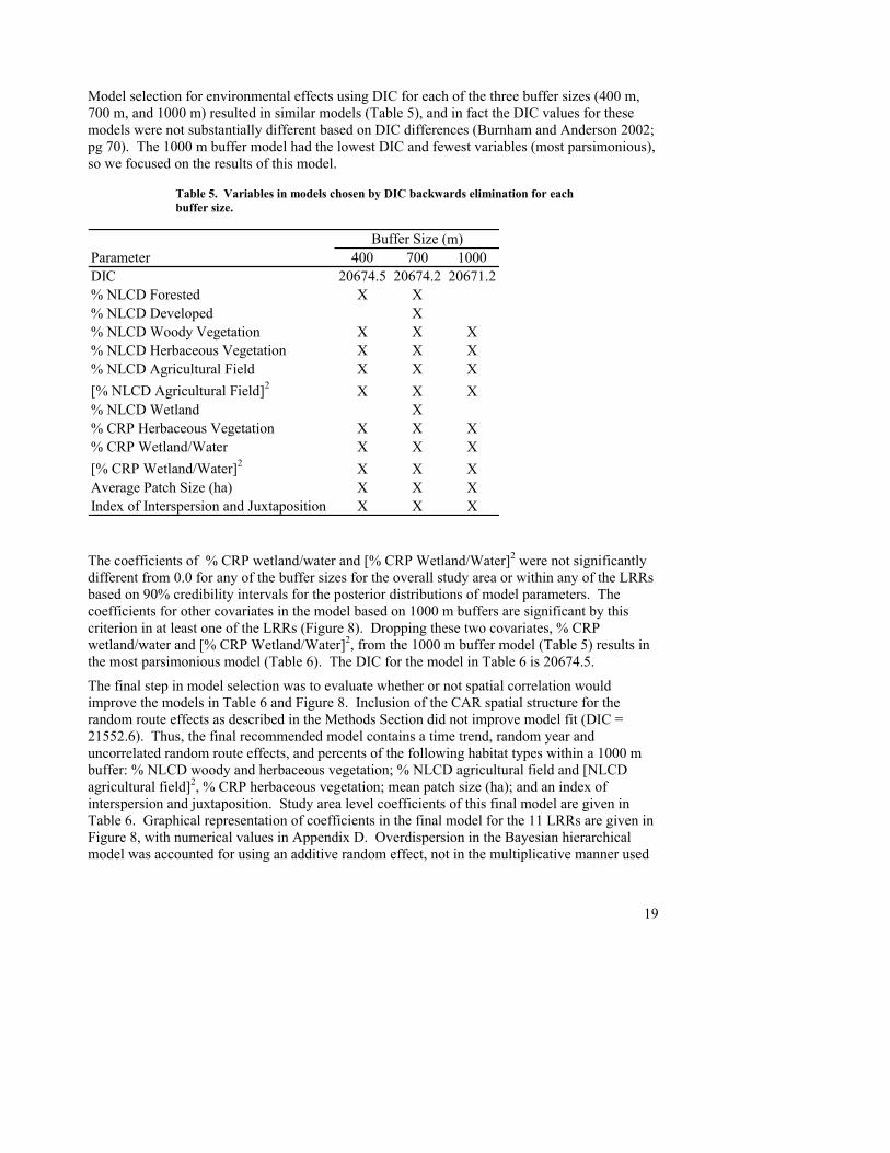
Model selection for environmental effects using DIC for each of the three buffer sizes (400 m, 700 m, and 1000 m) resulted in similar models (Table 5), and in fact the DIC values for these models were not substantially different based on DIC differences (Burnham and Anderson 2002; pg 70). The 1000 m buffer model had the lowest DIC and fewest variables (most parsimonious), so we focused on the results of this model.
Table 5. Variables in models chosen by DIC backwards elimination for each buffer size.
Parameter 400 700 1000DIC 20674.5 20674.2 20671.2% NLCD Forested X X% NLCD Developed X% NLCD Woody Vegetation X X X% NLCD Herbaceous Vegetation X X X% NLCD Agricultural Field X X X[% NLCD Agricultural Field]2 X X X% NLCD Wetland X% CRP Herbaceous Vegetation X X X% CRP Wetland/Water X X X[% CRP Wetland/Water]2 X X XAverage Patch Size (ha) X X XIndex of Interspersion and Juxtaposition X X X
Buffer Size (m)
The coefficients of % CRP wetland/water and [% CRP Wetland/Water]2 were not significantly different from 0.0 for any of the buffer sizes for the overall study area or within any of the LRRs based on 90% credibility intervals for the posterior distributions of model parameters. The coefficients for other covariates in the model based on 1000 m buffers are significant by this criterion in at least one of the LRRs (Figure 8). Dropping these two covariates, % CRP wetland/water and [% CRP Wetland/Water]2, from the 1000 m buffer model (Table 5) results in the most parsimonious model (Table 6). The DIC for the model in Table 6 is 20674.5.
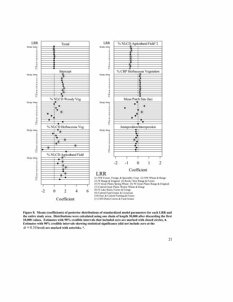
The final step in model selection was to evaluate whether or not spatial correlation would improve the models in Table 6 and Figure 8. Inclusion of the CAR spatial structure for the random route effects as described in the Methods Section did not improve model fit (DIC = 21552.6). Thus, the final recommended model contains a time trend, random year and uncorrelated random route effects, and percents of the following habitat types within a 1000 m buffer: % NLCD woody and herbaceous vegetation; % NLCD agricultural field and [NLCD agricultural field]2, % CRP herbaceous vegetation; mean patch size (ha); and an index of interspersion and juxtaposition. Study area level coefficients of this final model are given in Table 6. Graphical representation of coefficients in the final model for the 11 LRRs are given in Figure 8, with numerical values in Appendix D. Overdispersion in the Bayesian hierarchical model was accounted for using an additive random effect, not in the multiplicative manner used
20
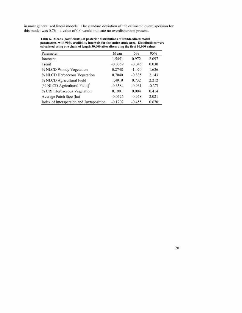
in most generalized linear models. The standard deviation of the estimated overdispersion for this model was 0.76 – a value of 0.0 would indicate no overdispersion present.
Table 6. Means (coefficients) of posterior distributions of standardized model parameters, with 90% credibility intervals for the entire study area. Distributions were calculated using one chain of length 30,000 after discarding the first 10,000 values.
Parameter Mean 5% 95%Intercept 1.5451 0.972 2.097Trend -0.0059 -0.045 0.030% NLCD Woody Vegetation 0.2748 -1.070 1.636% NLCD Herbaceous Vegetation 0.7040 -0.835 2.143% NLCD Agricultural Field 1.4919 0.732 2.212[% NLCD Agricultural Field]2 -0.6584 -0.961 -0.371% CRP Herbaceous Vegetation 0.1991 0.004 0.414Average Patch Size (ha) -0.0526 -0.958 2.021Index of Interspersion and Juxtaposition -0.1702 -0.455 0.670
21
-2 0 2 4 6
Coefficient
Trend
Intercept
% NLCD Woody Veg
% NLCD Herbaceous Veg
% NLCD Agricultural Field
1110987654321
Study -Area
1110987654321
Study -Area
1110987654321
Study -Area
1110987654321
Study -Area
1110987654321
Study -Area
LRR
% NLCD Agricultural Field^2
% CRP Herbaceous Vegetation
Mean Patch Size (ha)
Juxtaposition/Interspersion
1110987654321
Study -Area
1110987654321
Study -Area
1110987654321
Study -Area
1110987654321
Study -Area
LRR
-2 -1 0 1 2
CoefficientLRR
(1) NW Forest, Forage, & Speciallty Crop (2) NW Wheat & Range(3) W Range & Irrigated (4) Rocky Mnt Range & Forest(5) N Great Plains Spring Wheat (6) W Great Plains Range & Irrigated(7) Central Great Plains Winter Wheat & Range(8) N Lake States Forest & Forage(9) Central Feed Grains & Livestock(10) East & Central Farming & Forest(11) MS Delta Cotton & Feed Grains
Figure 8. Means (coefficients) of posterior distributions of standardized model parameters for each LRR and the entire study area. Distributions were calculated using one chain of length 30,000 after discarding the first 10,000 values. Estimates with 90% credible intervals that included zero are marked with closed circles, ●. Estimates with 90% credible intervals showing statistical significance (did not include zero at the
0.10α = level) are marked with asterisks, *.
22
We standardized environmental covariates (subtraction of the mean and division by the standard deviation) for the Bayesian hierarchical model. Ease of interpretation of the environmental coefficients in the final model is improved by use of the average and standard deviation of each covariate (Table 7).
Table 7. Average and standard deviation of environmental variables that appear in the final model of BBS counts of ring-necked pheasants. Units of the first four variables are % of 1000 m buffer. Mean patch size is in hectares. The index of interspersion and juxtaposition has no defined units.
Variable Average Standard Deviation% NLCD Woody Vegetation 11.725 22.384% NLCD Herbaceous Vegetation 32.655 23.322% NLCD Agricultural Field 30.904 27.652% CRP Herbaceous Vegetation 2.461 4.048Mean Patch Size (ha) 4.122 4.017Index of Interspersion and Juxtaposition 45.895 15.742
% of 1000 m Buffer
Predicted effects of increases in CRP herbaceous vegetation on BBS counts of ring-necked pheasants were calculated by identifying the average habitat conditions within a 1000 m buffer along a route in each LRR, and computing the predicted count based on those average conditions and with a 319 hectare (788 acre; 1 standard deviation) increase in CRP herbaceous vegetation (Table 8). Estimated effects for all environmental variables in each LRR are provided in Appendix D.
23
Table 8. Predicted BBS counts of ring-necked pheasant along a route with average conditions within the region, and the effects of CRP herbaceous vegetation within each LRR. First, we predicted BBS ring-necked pheasant counts along a route with average conditions for each LRR and the study area. Using the estimated “coefficient” of % CRP herbaceous vegetation in the final model, which is the mean of the posterior distribution of the model coefficient, an increase in pheasant counts was predicted along the route given a 319 ha (788 acre; 1 standard deviation) increase in CRP herbaceous vegetation. A similar sized decrease can be expected for a 319 ha reduction in CRP herbaceous vegetation.
Coefficient for Predicted Count Hectares of CRP Predicted Count% CRP Herbaceous Along Herbaceous Vegetation Following 319 ha
LRR Vegetation Average Route Along Average Route Increase in CRPStudy Area 0.199* 4.7 194.1 5.7
1 0.178 1.1 1.1 1.42 0.214 3.9 201.7 4.63 0.188 3.0 82.1 3.74 0.203 1.3 4.9 1.55 0.195 0.8 333.4 0.96 0.206 28.7 144.8 34.87 0.227* 32.6 366.8 40.18 0.203 1.1 50.8 1.49 0.173 6.2 321.7 7.6
10 0.199 0.8 164.0 1.011 0.202 50.9 0.0 62.1
*Estimates with 90% credible intervals showing statistical significance at 0.10α = .
Due to small sample sizes, predictions for regions 10 and 11 are suspect.
A marginal plot was created to aid interpretation of the model parameters for % CRP herbaceous vegetation (Figure 9). This plot was created by predicting BBS ring-necked pheasant counts for an average route within each LRR. Holding amounts of all other habitat types constant, we predicted BBS pheasant counts for various levels of CRP herbaceous vegetation. The range of values used for % CRP herbaceous vegetation was based on observed values within each LRR. Based on the average 1000 m buffer around a 24.5 mile route (7886 ha), 10 % CRP is equivalent to approximately 789 ha (1950 acres), and 20% CRP is equivalent to 1577 ha (3897 acres).
24
05
1015
2025
30
% CRP Herbaceous Vegetation
BB
S Ph
easa
nt C
ount
0 10 20 27
Study AreaLRR 1LRR 2LRR 3LRR 4LRR 5
LRR 6LRR 7LRR 8LRR 9LRR 10LRR 11
Figure 9. Predicted BBS pheasant counts for the average route in each LRR and the study area for a range of values of % CRP herbaceous vegetation within a 1000 m buffer.
Model Evaluation The posterior predictive p-value for the final model was 0.664, which is close to 0.5, indicating reasonable fit of the model to the observed data. Using the final model (Table 6, Figure 8) based on habitat amounts within a 1000 m buffer around each BBS route, we dropped all BBS counts in 2005 and re-fit the model using the same number of MCMC iterations. This re-estimated model was then used to predict BBS pheasant counts in 2005. Model predictions were highly correlated with the observed counts along each route (Pearson’s correlation coefficient r = 0.827) (Figure 10).
25
0 50 100 150 200
050
100
150
200
Predicted Count
BB
S Ph
easa
nt C
ount
Figure 10. Ring-necked pheasant counts along 200 routes surveyed in 2005 versus counts predicted by the final model re-estimated using 1987 – 2004 data. The dotted line represents a one-to-one relationship. The solid line represents the linear relationship estimated by least-squares regression.
A fixed effects model with the same environmental covariates estimated using SAS Proc Genmod (SAS Institute 2000) had coefficients very similar to study area coefficients in the Bayesian hierarchical model (Table 9). Ninety-percent credible intervals for hierarchical model coefficients showed all but one of the estimates (intercept) were not significantly different from each other at the 0.10α = level.
Table 9. Coefficients estimated with a fixed effects model in SAS versus the Bayesian hierarchical model estimated using MCMC.
SAS FixedParameter Effects Model Study Area Coefficient 5% 95%Intercept 2.710 1.5451 0.972 2.097Trend 0.007 -0.0059 -0.045 0.030% NLCD Woody Vegetation 0.455 0.2748 -1.070 1.636% NLCD Herbaceous Vegetation 0.725 0.7040 -0.835 2.143% NLCD Agricultural Field 1.277 1.4919 0.732 2.212[% NLCD Agricultural Field]2 -0.355 -0.6584 -0.961 -0.371% CRP Herbaceous Vegetation 0.175 0.1991 0.004 0.414Mean Patch Size (ha) -0.037 -0.0526 -0.958 2.021Index of Interspersion and Juxtaposition -0.081 -0.1702 -0.455 0.670
Bayesian Hierarcichal Model
26
Discussion
Use of the DIC criterion in fitting Bayesian Hierarchical Modes Little is known about the ability of the DIC criterion to select the most parsimonious model, but our experience is that its frequentist equivalent, AIC, tends to over fit the available data by including too many covariates. Employing too many covariates in standard frequentist regression modeling includes coefficients associated with relatively small improvements in the AIC tending to fit extreme values in the available data and hence may not accurately fit the general trend of other or future data. This potential for over-fitting led us to selection of a parsimonious model guided by DIC rather than a strict adherence to the DIC criterion.
Model selection by DIC in this report seemed to favor models with larger numbers of covariates, regardless of the fact that we dropped CRP wetland/water based on lack of statistical significance in any LRR. We were concerned that the models selected may not predict new data very well, because of the large number of covariates included. Our check for adequacy of the final model was to drop the 2005 ring-necked pheasant BBS counts, refit the model based on pre-2005 counts, use the refitted model to predict the 2005 counts route by route, and consider the correlation of the observed and predicted counts (Figure 10). The re-fitted model tended to underestimate the observed ring-necked pheasant counts in 2005, because the estimated random effect of 2005 was positive (Table D.2). The correlation was, never-the-less, quite good (0. 827). For this reason, we feel comfortable recommending use of the final models (Figure 8 and Appendix D). Recall that the coefficients of the final model were obtained using BBS data through 2005.
Based on smaller-scale studies, ring-necked pheasants have been positively correlated with CRP practices (Eggebo et al. 2003, Patterson and Best 1996). Some studies have shown that pheasants seem to prefer wetland habitats in some areas during specific seasons. Percent CRP wetlands was dropped from the 1000 m buffer model (Table 5) selected by DIC because estimates of the effects of wetlands were not significantly different from zero within any individual LRR, or across the study area as a whole. However, CRP enrollment types CP23 and CP27 (Table 1) were not available until 1997, so wetland habitats enrolled prior to 1997 were likely enrolled as grasses (CP1, CP2, CP10; pers. comm. Skip Hyberg, FSA). This possibly obscured any effect of CRP wetlands discernable in our analysis.
Interpretation of the Recommended Model The models presented in this report were derived from relationships observed in the available data. As in the use of all empirical models, it is advisable to remember three principles that have been highlighted by McCullagh and Nelder (1983), among others. These are:
All models are wrong, but some are useful, Modeling in science is at least partly an art rather than a completely objective process,
and
It is not a good idea to fall in love with one model to the exclusion of alternatives. To these we would add the corollary:
Empirical models do not last very long.
27
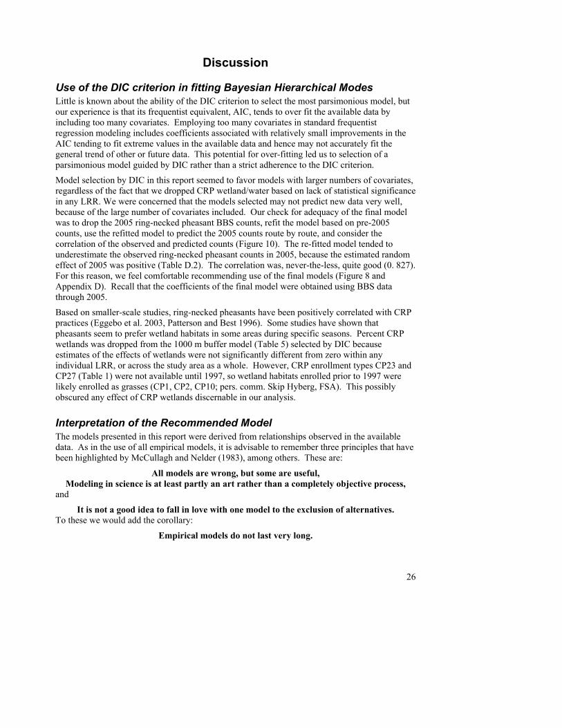
Empirical models are estimated with the basic objective of providing predictions that come as close to the observed data values as possible. In general, one can expect several different sets of covariates to do about equally well in fitting the available data, and so we caution the reader from putting too much importance on which covariates ended up in the recommended model. For example, a model with “total % CRP” (which includes wetlands, trees, woody and herbaceous vegetation) was found to predict BBS ring-necked pheasant counts nearly as well as the model containing only “CRP herbaceous vegetation” (when combined with the other NLCD covariates) (r = 0.826; Figure 11). Thus, we cannot conclude ring-necked pheasants do not benefit from other CRP practices besides those falling in the herbaceous vegetation class. However, we have presented a useful model for predicting ring-necked pheasant counts in the BBS. This model predicts an increase in ring-necked pheasant counts for given increases in hectares of CRP herbaceous vegetation, and is viewed as reliable, provided we do not extrapolate beyond the range of observed values (amount of CRP within a 1000 m buffer) of CRP in the available data and other conditions remain similar.
0 50 100 150 200
050
100
150
200
Predicted Count
BB
S Ph
easa
nt C
ount
Figure 11. Ring-necked pheasant counts along 200 routes surveyed in 2005 versus counts predicted by a model with % total CRP in place of % CRP herbaceous vegetation. This model was estimated using 1987 – 2004 data. The dotted line represents a one-to-one relationship. The solid line represents the linear relationship estimated by least-squares regression.
Tables 6 and 7 can be used to interpret the estimated relationships. For example, across the study area, there is an estimated (Table 6) exp(0.1991) = 1.22 fold, or 22%, increase in ring-necked pheasant counts along a BBS route associated with a 1 standard deviation increase (4.05 %; Table 7), in percent of CRP herbaceous vegetation within a 1000 m buffer, holding other variables constant. Using the median pheasant count along a route (i.e., the count of 6), and the
28
average buffer size along a 24.5 mile route (7886 acres), we can simplify the above interpretation and say there is an estimated average increase of 1.32 BBS ring-necked pheasant counts for every additional 319 ha (788 acres) of CRP herbaceous vegetation within a 1000 m buffer during 1987 – 2005. A similar sized decrease (-22%) can be expected for a 319 ha reduction in CRP herbaceous vegetation. An example of how to calculate a prediction for a specific BBS route based on the final model is presented in Appendix D.
Another way to interpret the effect of an increase in CRP herbaceous vegetation, would be that while holding all other variables constant, if enrollment in CRP herbaceous vegetation was increased by 4.05% in a random or uniform manner across the study area during 1987 – 2005, there would be an estimated average 22% increase in pheasant counts on randomly located BBS routes.
Using the final model (Table 6) for the entire study area as an illustration, there is an indication of a slight decline in pheasant numbers across the entire study area since 1987 (trend over years is slightly negative but not significant). Similarly, the final model leads to the strong conjecture:
1. positive relationships for ring-necked pheasant counts along BBS routes associated with larger amounts of NLCD 1992 woody and herbaceous vegetation,
2. an estimated decrease in ring-necked pheasant counts along BBS routes in areas with large patches of habitat as defined by our NLCD and CRP cover types, and
3. decreases associated with increases in the index of interspersion and juxtaposition.
In comparison, the estimated positive effects of NLCD 1992 agricultural fields and CRP herbaceous vegetation were significant at the 0.1α = level and deserve more consideration.
The final model is based on past data and statistical relationships. Predictions are appropriate to what would have happened to BBS pheasant counts given changes in enrollment of CRP herbaceous vegetation during 1987 – 2005, while holding other variables constant. Future predictions or predictions involving changes in more than one variable are always tentative. The model may not accurately account for future events or the effects of complicated interactions between variables.
Comparisons across LRRs show little variation in the estimated effect of CRP herbaceous vegetation on BBS counts of ring-necked pheasants (Table 8, Figures 8 and 9). All region specific coefficients are positive, are of about the same magnitude, and several are significant. Also, the estimated effects of NLCD agricultural field were very consistent across LRRs. Estimated effects of the other NLCD habitat types were more variable across regions (Figure 8) and should be given less consideration in interpreting predictions of the final model.
Estimates of effects of % NLCD 1992 woody and herbaceous vegetation, and mean patch size, exhibited higher than expected variation across LRRs (Figure 8), possibly indicating that separate models should be determined for each region (i.e., allowing different model parameters), provided more data were available for each region. NLCD 1992 woody vegetation was rare in the data with the exception of routes within 4 LRRs: (1) Northwestern Forest, Forage, and Specialty Crop; (2) Northwestern Wheat and Range; (3) Western Range and Irrigated; and (4) Rocky Mountain Range and Forest.
Formatted: Space After: 0 pt
Formatted: Bullets and Numbering
Deleted: of
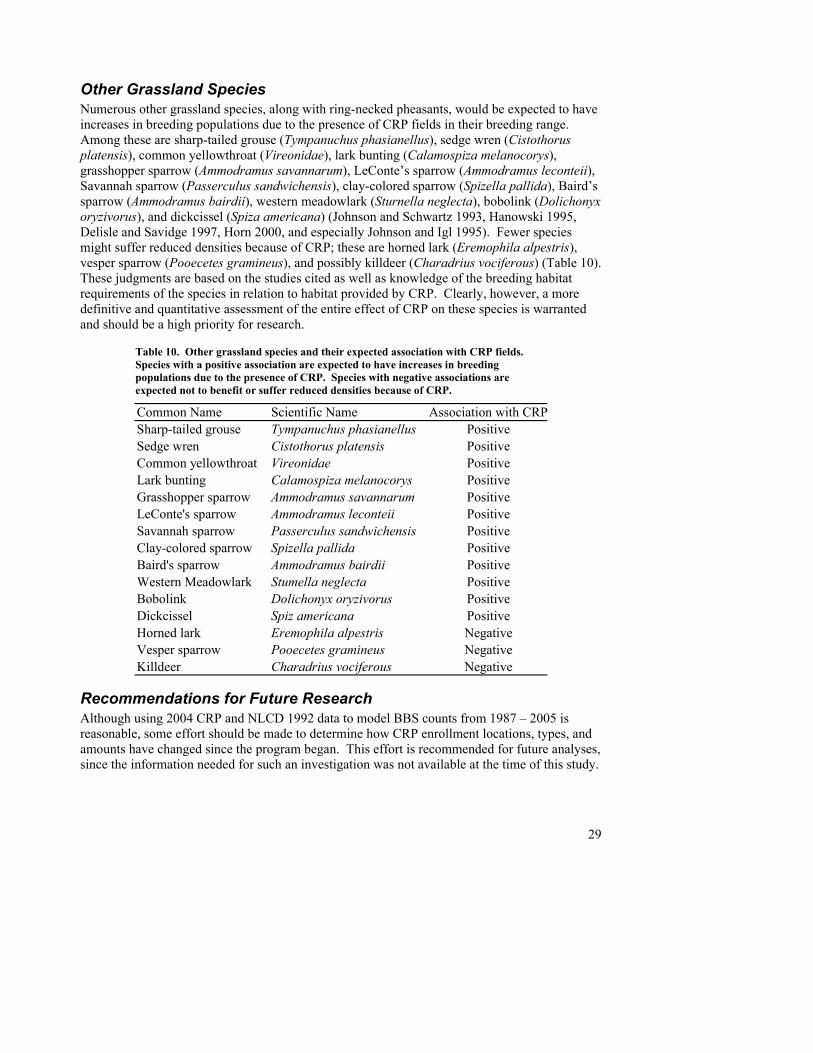
29
Other Grassland Species Numerous other grassland species, along with ring-necked pheasants, would be expected to have increases in breeding populations due to the presence of CRP fields in their breeding range. Among these are sharp-tailed grouse (Tympanuchus phasianellus), sedge wren (Cistothorus platensis), common yellowthroat (Vireonidae), lark bunting (Calamospiza melanocorys), grasshopper sparrow (Ammodramus savannarum), LeConte’s sparrow (Ammodramus leconteii), Savannah sparrow (Passerculus sandwichensis), clay-colored sparrow (Spizella pallida), Baird’s sparrow (Ammodramus bairdii), western meadowlark (Sturnella neglecta), bobolink (Dolichonyx oryzivorus), and dickcissel (Spiza americana) (Johnson and Schwartz 1993, Hanowski 1995, Delisle and Savidge 1997, Horn 2000, and especially Johnson and Igl 1995). Fewer species might suffer reduced densities because of CRP; these are horned lark (Eremophila alpestris), vesper sparrow (Pooecetes gramineus), and possibly killdeer (Charadrius vociferous) (Table 10). These judgments are based on the studies cited as well as knowledge of the breeding habitat requirements of the species in relation to habitat provided by CRP. Clearly, however, a more definitive and quantitative assessment of the entire effect of CRP on these species is warranted and should be a high priority for research.
Table 10. Other grassland species and their expected association with CRP fields. Species with a positive association are expected to have increases in breeding populations due to the presence of CRP. Species with negative associations are expected not to benefit or suffer reduced densities because of CRP.
Common Name Scientific Name Association with CRPSharp-tailed grouse Tympanuchus phasianellus PositiveSedge wren Cistothorus platensis PositiveCommon yellowthroat Vireonidae PositiveLark bunting Calamospiza melanocorys PositiveGrasshopper sparrow Ammodramus savannarum PositiveLeConte's sparrow Ammodramus leconteii PositiveSavannah sparrow Passerculus sandwichensis PositiveClay-colored sparrow Spizella pallida PositiveBaird's sparrow Ammodramus bairdii PositiveWestern Meadowlark Stumella neglecta PositiveBobolink Dolichonyx oryzivorus PositiveDickcissel Spiz americana PositiveHorned lark Eremophila alpestris NegativeVesper sparrow Pooecetes gramineus NegativeKilldeer Charadrius vociferous Negative
Recommendations for Future Research Although using 2004 CRP and NLCD 1992 data to model BBS counts from 1987 – 2005 is reasonable, some effort should be made to determine how CRP enrollment locations, types, and amounts have changed since the program began. This effort is recommended for future analyses, since the information needed for such an investigation was not available at the time of this study.
30
Alternative definitions of unique patches of habitat types could be more meaningful to pheasants and thus provide more appropriate measures of mean patch size and interspersion and juxtaposition. For example, pheasants may only benefit from interspersion and juxtaposition of agricultural field and woody and herbaceous vegetation, not interspersion and juxtaposition of all 14 NLCD and CRP types used in this analysis.
Model building could be conducted to allow for variables represented at various buffer sizes. Thus, a model could potentially contain predictor variables measured in a 400 m buffer, others measured in a 700 m buffer, and so on. Justification for this “multi-scale” model is that pheasants might select habitat based on different landscape scales for different habitat characteristics.
It might be possible to produce useful models of ring-necked pheasant counts based only on CRP practices, a time trend, random year and route effects, and using the CAR spatial structure to pick up any unexplained differences among routes with respect to NLCD. That is, the CAR spatial structure may be able to account for variation in the NLCD image yielding simpler models dependent only on CRP data.
Availability of Data and Refitting of Models Data available for this analysis represents a substantial, but incomplete, selection from the range of ring-necked pheasants in the US (Figures 1 and 4). The methods described above, including re-selection of covariates, can be re-applied when data on CRP enrollments are available from additional states. The distribution of CRP enrollment by type varies spatially, so we would expect that modeling ring-necked pheasant counts along BBS routes might require inclusion of CRP trees, CRP woody vegetation, or CRP wetland classes in other areas of the country.
The NLCD 1992 covers the entire lower 48 states with a consistent approach and definitions. However, this coverage is becoming outdated given that it is based on Landsat or aerial images from 1992. The NLCD is being updated based on 2001 images, but the update will not be completed until 2006 or later (pers. comm. Stephen Howard, USGS EROS Data Center). We recommend re-running the analysis, including variable selection, using the NLCD 2001 image once it becomes available for states for which CRP data are available.
If additional data are added to those used in this analysis, environmental variables should be re-standardized based on the average and standard deviation of the complete data set. In addition, if model validation involves routes not used in the analysis, or the landscape has changed along those routes over time, the environmental variables for those routes need to be standardized using the same transformation applied to the model data. The spatial covariance structure for random route effects should be investigated in future analyses, when additional CRP and NLCD 2001 data are available.
The methods outlined above could also be used to evaluate the effects of CRP practices on BBS counts of other species. If a species is rare or difficult to detect, visually or audibly, a random observer effect could be included in the hierarchical model, and a fixed effect for novice observers should also be investigated (Thogmartin et al. 2004b; 2006).
The Bayesian hierarchical model simultaneously provides estimates for the entire study area and each LRR. Those LRRs with smaller sample sizes provide less information for study area parameter estimates compared to larger sample sizes from other regions, and their specific
31
posterior distributions are closer to the hyperparameters’ posteriors because they essentially borrow information from regions with more observations. Due to small sample sizes, parameter estimates for the East and Central Farming and Forest region (10) and the Mississippi Delta Cotton and Feed Grains region (11) should not be used to make bold predictions within those regions.
References Barbarika, A., S. Hyberg, J. Williams, and J. Agapoff. 2004. Conservation Reserve Program
Overview. CRP: Planting for the future. United States Department of Agriculture, Farm Service Agency. Washington DC. x + 25 pp.
Bart, J., M. Hopschen, B.G. Peterjohn. 1995. Reliability of the Breeding Bird Survey: Effects of
restricting surveys to roads. Auk 112: 758-761. Burnham, K. P., and D. R. Anderson (2002). Model Selection and Multimodel Inference.
Second edition. Springer, New York, New York, USA. Bystrak, D. 1981. The North American Breeding Bird Survey. Studies in Avian Biology 6: 34-41.
Bystrak, D. 1981. The North American Breeding Bird Survey. Pages 34 – 41 in C. J. Ralph and
J. M. Scott, editors. Estimating numbers of terrestrial birds. Studies in Avian Biology 6. Delisle, J. M., and J. A. Savidge. 1997. Avian use and vegetation characteristics of Conservation
Reserve Program fields. Journal of Wildlife Management 61:318–325. Eggebo, S. L., K. F. Higgins, D. E. Naugle, and F. R. Quamen. 2003. Effects of CRP field age
and cover type on ring-necked pheasants in eastern South Dakota. Wildlife Society Bulletin 31:779 – 785.
Friedman, J. H. 1984. SMART User’s Guide. Laboratory for Computational Statistics, Stanford
University Technical Report No. 1. Gelman, A., and X. L. Meng. 1996. Model checking and model improvement. Pages 189 – 201
in W. R. Gilks, S. Richardson, and D. J. Spiegelhalrter, editors. Markov chain Monte Carlo Methods in practice. Chapman & Hall, New York, USA.
Gilks, W. R., and G. O. Roberts. 1996. Strategies for improving MCMC. Pages 89-114 in W.
R. Gilks, S. Richardson, and D. J. Spiegelhalrter, editors. Markov chain Monte Carlo methods in Practice. Chapman & Hall, New York, USA.
Giudice, J. H., and J. T. Ratti. 2001. Ring-necked Pheasant (Phasianus colchicus). In The Birds
of North America, No. 572 (A. Poole and F. Gill, eds.). The Birds of North America, Inc., Philadelphia, PA.
Gough, G.A., J. R. Sauer, M. Iliff. 1998. Patuxent Bird Identification Infocenter. 1998. Version
97.1. Ptuxent Wildlife Research Center, Laurel, MD. http://www.mbr-pwrc.usgs.gov/id/framlst/infocenter.html.
32
Hames, R.S., K.V. Rosenberg, J.D. Lowe, S.E. Barker, and A.A. Dhondt. 2002. Adverse effects
of acid rain on the distribution of the wood thrush Hylocichla mustelina in North America. Proceedings of the National Academy of Science 99: 11235-11240.
Hanowski, J.M. and G.J. Niemi (1995). A comparison of on- and off-road bird counts: Do you
need to go off road to count birds accurately. Journal of Field Ornithology 66(4) 469-483.
Hanowski, J.M. 1995. Breeding bird composition and species relative abundance patterns on
Conservation Reserve Program (CRP) land in western Minnesota. Loon 67:12–16. Horn, D. J. 2000. The influence of habitat features on grassland birds nesting in the Prairie
Pothole Region of North Dakota. Ph.D. Dissertation, Iowa State University, Ames, USA. Johnson, D. H., and M. D. Schwartz. 1993. The Conservation Reserve Program and grassland
birds. Conservation Biology 7:934–937. Johnson, D. H., and L. D. Igl. 1995. Contributions of the Conservation Reserve Program to
populations of breeding birds in North Dakota. Wilson Bulletin 107:709–718. Link, W. A., and J. R. Sauer. 1994. Estimating equations estimates of trends. Bird Populations
2:23 – 31. Link, W. A., E. Cam, J. D. Nichols, and E. G. Cooch. 2002. Of BUGS and birds: Markov chain
Monte Carlo for hierarchical modeling in wildlife research. Journal of Wildlife Management 6:277 – 291.
Link, W. A., and J. R. Sauer. 2002. A hierarchical analysis of population change with
application to cerulean warblers. Ecology 83:2832 – 2840. McCullagh, P., and J. A. Nelder. 1983. Generalized Linear Models. Chapman and Hall, London.
McCullagh, P. and J. A. Nelder. 1989. Generalized linear models. Second edition. Chapman and
Hall, Boca Raton, Florida, USA. McGarigal, K., and B. Marks. 1985. FRAGSTATS: Spatial pattern analysis program for
quantifying landscape structure. USDA Forest Service - General Technical Report PNW-GTR-351. http://www.innovativegis.com/basis/Supplements/BM_Aug_99/FRAG_expt.htm.
Moran, P. A. P. 1948. The interpretation of statistical maps. Journal of the Royal Statistical
Society B 10:243 – 251. Neter, J., M. H. Kutner, C. J. Nachtsheim, and W. Wasserman. 1996. Applied linear statistical
models. Fourth edition. McGraw-Hill, Boston, Massachusetts, USA.
33
Patterson, M. P, and L. B. Best. 1996. Bird abundance and nesting success in Iowa CRP fields: The importance of vegetation structure and composition. American Midland Naturalist 135:153 – 167.
R Development Core Team. 2005. R: A language and environment for statistical computing. R
Foundation for Statistical Computing, Vienna, Austria. ISBN 3-900051-07-0, URL http://www.R-project.org.
Raftery, A. E., and S. M. Lewis. 1992. One long run with diagnostics: Implementation
strategies for Markov chain Monte Carlo. Statistical Science 7:493 – 497. Ridgely, R.S., T.F.Allnutt, T. Brooks, D.K. McNicol, D.W.Mehlman, B.E. Young, and J.R.
Zook. 2003. Digital distribution maps of the birds of the Western Hemisphere, version 1.0. NatureServe, Arlington, VA. USA.
SAS Institute, Inc. 2000. SAS/STAT Users Guide. SAS Institute, Cary, North Carolina, USA. Sauer, J. R., J. E. Hines, and J. Fallon. 2001. The North American Breeding Bird Survey,
Results and Analysis 1966 - 2000. Version 2001.2, USGS Patuxent Wildlife Research Center, Laurel, MD.
Sauer, J. R., and W. A. Link. 2002. Hierarchical modeling of population stability and species
group attributes from survey data. Ecology 86:1743 – 1751. Speigelhalter, D. J., A. Thomas, N. B. Best, and D. Lunn. 2003a. WinBUGS Version 1.4. User
manual. MRC Biostatistics Unit, Cambridge, UK. Speigelhalter, D. J., N. G. Best, B. P. Carlin, and A. Van der Linde. 2003b. Bayesian measures
of model complexity and fit (with discussion). Journal of the Royal Statistical Society, Series B 64:583 – 616.
Thogmartin, W. E., A. L. Gallant, M. G. Knutson, T. J. Fox, and M. J. Suarez. 2004a.
Commentary: a cautionary tale regarding use of the National Land Cover Dataset 1992. Wildlife Society Bulletin 2004:970 – 978.
Thogmartin, W. E., J. R. Sauer, and M. G. Knutson. 2004b. A hierarchical spatial model of
avian abundance with application to cerulean warblers. Ecological Applications 14:1766 – 1779.
Thogmartin, W. E., M. G. Knutson, and J. R. Sauer. 2006. Predicting regional abundance of
rare grassland birds with a hierarchical spatial count model. Condor 108:25 – 46.
34
Appendix A: Data Methods
BBS Data – Acquisition North American BBS digitized route locations and locations of the route start points were available from the Bird Conservation Node of the National Biological Information Infrastructure (http://mbirdims.fws.gov/nbii/). By following the link to “Download GIS Data”, files compatible with ESRI’s ArcGIS or ArcInfo could be downloaded for the entire route lengths or just the start points. The route files were used to create buffers around each route.
Bird count data are available from the U.S. Geological Survey’s Patuxent Wildlife Research Center’s website (http://www.pwrc.usgs.gov). Following the links through Research → Birds → Breeding Bird Survey → Raw Data → “I have read the disclaimer . . “→ FTP Site → States will get to the page for downloading each state’s or province’s data. The data for each state or province can then be downloaded as either a comma-delimited or fixed-width data set. Additional files that define the codes that appear in the raw data or provide additional descriptions for routes and conditions of each survey also are available at this website on the web page that contains the link leading to the states page.
BBS Data – Description The data file for each state consists of an 11-column table providing in order from left to right, the state number, route number, year, American Ornithologists’ Union (AOU) species code, five columns containing the total counted for that species in 10 stop increments, number of stops where the species was counted, total number of individuals observed in all fifty stops. There is a single record within the data set for each species for each year it was observed along each route. When a particular species was not observed in a specific year, even if it had been observed in other years, no record appears in the data set.
The states and provinces are numbered in alphabetical order with all U.S states and Canadian provinces intermixed. The names of species and the codes that refer to them can be found in a file named “sAou.txt”. Additional files contained information required for the final analyses. The file “FRoutes.exe” can be expanded to “routes.txt” which contains the route name, whether the route is still active, its latitude and longitude, BBS physiographic stratum code, and the Bird Conservation Region for that route. The file “FWeather.exe” can be expanded to “weather.txt which contains a record for each year a route was surveyed. Each record in weather.txt contains the day and month the route was surveyed, a code for the observer for that year, weather conditions during the survey, start and stop times of the survey, whether the observer had an assistant, and whether that particular survey met all criteria and was acceptable for use in any analyses of the data.
BBS Data – Processing The BBS data contained variables for a state code as well as a route code. The state code was up to two digits (e.g., 1 – 99) and the route code was up to three digits (e.g., 1 – 999). To create a unique identifier for each route across all states, these codes needed to be combined. This was
35
accomplished after importing the data into Microsoft Access . A new variable, RouteNumber, was created by multiplying the state code by 1000 and then adding the route code. For example, the state code for Kansas is 38. Within Kansas, each route code was added to 38000 resulting in a unique RouteNumber that would not occur in any other state.
Inserting Records for Zero Observations Since no records were present in the BBS data to indicate years when the route was surveyed but no individuals of a species were observed, these records had to be created. To accomplish this, the BBS data were imported into Microsoft Access. One table was created within each state’s database that contained two variables RouteNumber and the species code, sAou with a single occurrence for each route X species combination. This was accomplished by:
1) Select the State BBS file Click “Copy” on the toolbar. 2) Click “Paste” on the toolbar. 3) In the Paste Table As dialog box, type “State Species by Route” for the copied table,
click Structure Only, and then click OK. 4) Open the new table in Design view, and select the RouteNumber and sAou fields in the
State BBS table. 5) Click Primary Key on the toolbar to create a primary key based on the selected fields. 6) Save and close the table. 7) Create a new query based on the State BBS table. 8) In query Design view, click Query Type on the toolbar, and then click Append Query. 9) In the Append dialog box, click the name of the new table in the Table Name list, and
then click OK. 10) Select only the RouteNumber and sAou fields from the State BBS table. 11) Run the query.
A second table was created in the same manner that consisted of only the RouteNumber and year using the same procedures. This table consisted of all the years in which each route was surveyed and was named “State Route by Year”. By combining the information in these two tables, it was possible to expand the dataset to create records that would include a record for each year a route was surveyed for all species that were ever observed on that route, whether or not they were observed during that particular year. This could not be accomplished in Microsoft Access, so the State BBS table and the two newly created tables were exported to STATA Statistical Data Analysis package.
Within STATA, the following procedures were used to combine the necessary tables and create the new records with zero values included when no individuals were observed in years when the route was surveyed.
1) Use “State Route by Year file”. 2) Join by using “State Species by Route file”, unmatched (both).
Files are joined on the common variable RouteNumber such that all possible combinations of RouteNumber, Year, and Species are created.
3) Save “State Species by Route by Year”. Copyright Microsoft Corportation Copyright StataCorp.
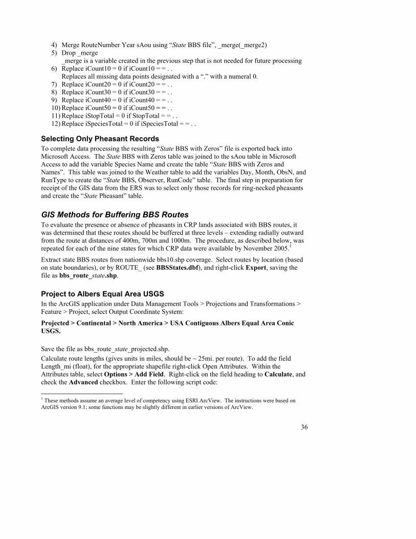
36
4) Merge RouteNumber Year sAou using “State BBS file”, _merge(_merge2) 5) Drop _merge
_merge is a variable created in the previous step that is not needed for future processing 6) Replace iCount10 = 0 if iCount10 = = . .
Replaces all missing data points designated with a “.” with a numeral 0. 7) Replace iCount20 = 0 if iCount20 = = . . 8) Replace iCount30 = 0 if iCount30 = = . . 9) Replace iCount40 = 0 if iCount40 = = . . 10) Replace iCount50 = 0 if iCount50 = = . . 11) Replace iStopTotal = 0 if StopTotal = = . . 12) Replace iSpeciesTotal = 0 if iSpeciesTotal = = . .
Selecting Only Pheasant Records To complete data processing the resulting “State BBS with Zeros” file is exported back into Microsoft Access. The State BBS with Zeros table was joined to the sAou table in Microsoft Access to add the variable Species Name and create the table “State BBS with Zeros and Names”. This table was joined to the Weather table to add the variables Day, Month, ObsN, and RunType to create the “State BBS, Observer, RunCode” table. The final step in preparation for receipt of the GIS data from the ERS was to select only those records for ring-necked pheasants and create the “State Pheasant” table.
GIS Methods for Buffering BBS Routes To evaluate the presence or absence of pheasants in CRP lands associated with BBS routes, it was determined that these routes should be buffered at three levels – extending radially outward from the route at distances of 400m, 700m and 1000m. The procedure, as described below, was repeated for each of the nine states for which CRP data were available by November 2005.1
Extract state BBS routes from nationwide bbs10.shp coverage. Select routes by location (based on state boundaries), or by ROUTE_ (see BBSStates.dbf), and right-click Export, saving the file as bbs_route_state.shp.
Project to Albers Equal Area USGS In the ArcGIS application under Data Management Tools > Projections and Transformations > Feature > Project, select Output Coordinate System:
Projected > Continental > North America > USA Contiguous Albers Equal Area Conic USGS.
Save the file as bbs_route_state_projected.shp. Calculate route lengths (gives units in miles, should be ~ 25mi. per route). To add the field Length_mi (float), for the appropriate shapefile right-click Open Attributes. Within the Attributes table, select Options > Add Field. Right-click on the field heading to Calculate, and check the Advanced checkbox. Enter the following script code:
1 These methods assume an average level of competency using ESRI ArcView. The instructions were based on ArcGIS version 9.1; some functions may be slightly different in earlier versions of ArcView.
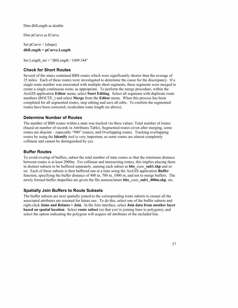
37
Dim dblLength as double
Dim pCurve as ICurve
Set pCurve = [shape] dblLength = pCurve.Length
Set Length_mi = “dblLength / 1609.344”
Check for Short Routes Several of the states contained BBS routes which were significantly shorter than the average of 25 miles. Each of these routes were investigated to determine the cause for the discrepancy. If a single route number was associated with multiple short segments, these segments were merged to create a single continuous route, as appropriate. To perform the merge procedure, within the ArcGIS application Editor menu, select Start Editing. Select all segments with duplicate route numbers (ROUTE_) and select Merge from the Editor menu. When this process has been completed for all segmented routes, stop editing and save all edits. To confirm the segmented routes have been corrected, recalculate route length (as above).
Determine Number of Routes The number of BBS routes within a state was tracked via three values: Total number of routes (based on number of records in Attributes Table), Segmented routes (even after merging, some routes are disjoint – especially “900” routes), and Overlapping routes. Tracking overlapping routes by using the Identify tool is very important, as some routes are almost completely collinear and cannot be distinguished by eye.
Buffer Routes To avoid overlap of buffers, subset the total number of state routes so that the minimum distance between routes is at least 2000m. For collinear and intersecting routes, this implies placing them in distinct subsets to be buffered separately, naming each subset as bbs_state_sub1.shp and so on. Each of these subsets is then buffered one at a time using the ArcGIS application Buffer function, specifying the buffer distance of 400 m, 700 m, 1000 m, and not to merge buffers. The newly formed buffer shapefiles are given the file nomenclature bbs_state_sub1_400m.shp, etc.
Spatially Join Buffers to Route Subsets The buffer subsets are next spatially joined to the corresponding route subsets to ensure all the associated attributes are retained for future use. To do this, select one of the buffer subsets and right-click Joins and Relates > Join. In the Join interface, select Join data from another layer based on spatial location. Select route subset (so that you’re joining lines to polygons), and select the option indicating the polygons will acquire all attributes of the included line.
38
Append Subsets Once the spatial join is complete, and it is confirmed that all attributes have been correctly associated with buffered routes, append the buffer subsets to a single shapefile within the ArcGIS application by selecting from Data Management Tools > General > Append (use TEST schema type).
Check for correct attributes, especially for overlapping routes. This can be done using the Identify tool.
Delete Extra Fields A number of the fields associated with the buffered routes are extraneous or all zeros, and should be deleted. The fields to be kept are as follows: FID, Shape, BufferDist, BBS_ROUTE_, ROUTE_, ROUTENAME, ACTIVE, STRATUM, BCR_REGION, ASSIGN2001, SOURCETHM, Shape_len (or LENGTH), Length_mi.
When this process is complete for a given state, export the appended buffer shapefile to a new shapefile named statebuff400m.shp, and so on. In the end there will be three buffer shapefiles for each state—statebuff400m.shp, statebuff700m.shp, statebuff1000m.shp.
Economic Research Service Background The general role that the Economic Research Service (ERS) fulfills regarding the Conservation Effects Assessment Project (CEAP) Wildlife Component project is to use Geographic Information System (GIS) and statistical methods to construct land use shares and landscape indices for areas around BBS routes. The project begins with base Common Land Unit (CLU) GIS data and associated CRP tables provided by Farm Services Agency (FSA) and BBS route-level buffer polygons provided by cooperating partners. ERS’s portion of the project ends with a state-level data set of land use shares and landscape indices for each BBS route. The work is completed in six phases.
Receipt of Conservation Reserve Program GIS Data from Farm Service Agency ERS was provided CRP Data from the FSA throughout 2005. As of November, 2005, ERS had received data for nine states that were used in the analysis. ERS received the data in two general formats.
The first format, referred to as version 1, included, for each county, CLU shapefiles and associated CRP tables. The CLU shapefiles contain boundaries for ALL farm fields. The CRP tables contained contract identifier and practice information. ERS received version 1 CLU shapefiles and associated CRP Tables for the following states: ID, ND, SD and most counties in MO.
The second format, referred to as version 2, included, for each county, CRP shapefiles. The CRP shapefiles contained boundaries for ONLY the CRP fields. The CRP shapefiles contained contract and practice information. Because the CRP shapefiles contained all necessary contract information, it was not necessary to merge them with CRP data. Version 2 data was received for the following states: KS, NE, MN, OR, and UT.

39
Version 2 represented an update to version 1. It was considerably cleaner and required little extra work. FSA verified all data in version 2 against the national CRP data base.
Phase 1. Standardizing, Projecting, and Merging County-Level CLU and CRP Shapefiles The version 1 CLU data were provided by FSA in the form of county-level ArcView shapefiles. For each state, the county-level CLU shapefiles were merged into one statewide shapefile so they can be combined with CRP contract data in Phase 2. The county-level shapefiles differed in projection and were converted to the USGS Albers Equal Area. The following is a step-by-step process for completing Phase 1 for the version 1 CLU shapefiles, including the names of associated SAS programs.
1) Place all county-level CLU shapefiles in directory …CLU\ST_CLU\OrigData. 2) Review all county-level CLU shapefiles to gather information on their projection (UTM
zones) and to test if they are usable. Opening the shapefiles in ArcView and displaying them was sufficient to ensure they were usable. A SAS program called “Extracting projection information.sas” was created to generate a list of the projection of each shapefile. In some instances, projection information was incorrect or non-existent and was corrected before proceeding.
3) Most of the county-level CLU shapefiles have consistent attribute information (contained in their associated .dbf file). However, various files contain extra information and, in some cases, inconsistent attribute names. In order to ensure proper merging of files in later steps, .dbf files were reformatted to contain consistent attribute names. This was accomplished by running the SAS code “SAS CODE FOR Fixing DBF to have same vars.sas”. Each state had its own version of this script. It is contained in …CLU\ST_CLU.
4) Merge county-level CLU shapefiles with same projection into single statewide CLU shapefile. This was accomplished using ArcGIS Append command. This process was run 2-3 times, depending on the number of separate projections in the county-level CLU shapefiles.
5) Re-project the new statewide CLU shapefiles to USGS Albers Equal Area. The new re-projected shapefile was stored in CLU\ST_CLU\CRPLayer and was named “joinedlayer_all_aea”.
The step-by-step process for completing Phase 1 for the version 2 CRP shapefiles followed the above procedures with a single exception. Since all the county-level CRP shapefiles have consistent attribute information (contained in their associated .dbf file), it was not necessary to perform Step 3.
Processing Conservation Reserve Program GIS Data
Phase 2. Creating CRP Layer for Version 1 (this Phase applies to Version 1 ONLY) Phase 1 yielded a single statewide CLU shapefile for version 1 states. From this CLU shapefile, we need to extract just the CLU’s that are CRP parcels. Accompanying the CLU shapefile data
40
are tables that provide information on which CLU’s are enrolled in the CRP program. There is one table per county. These tables are stored in the subdirectory ...CLU\ST_CLU\OrigData and are in DBF format. They were named “crp_t_ST###.dbf” by FSA where ST is the two letter state abbreviation and ### represents the 3-digit county code. These tables contain information on cover practice and contract expiration date. Some records in these tables were missing information, particularly in the cover practice field. This was troublesome as the analysis depends heavily on having correct cover practice for each field.
To fill in some of the missing information, ERS used the Fiscal Year 2002 and a monthly upload of June 2004 data from the national CRP contracts database. This national database contained all the information for each CRP contract. Two different points in time were used to maximize the chances of getting a match between the CRP data that accompanies the CLU and a record in the national data base2. Since the CRP data that accompany the CLU data contain contract numbers, the contract number can be used to link with the national database and fill in missing information when necessary. It is important to note that ERS assumed that the information contained in the CRP data that accompanies the CLU is correct. We use the national CRP data base ONLY when we have missing data.
To build the CRP table, ERS wrote a SAS program (Create CRP contract data.sas) for each state with version 1 data. The program does the following:
1) Imports and Appends all the CLU CRP Contract dbf files received from FSA. 2) Imports Fiscal Year 2002 and June 2004 national CRP contracts data. 3) Aggregates the CRP practices from the CRP Contract dbf, per instructions from
cooperating partners. 4) When CLU CRP Contract dbf files are missing CRP practice data, the practice data from
the FY 2002-June 2004 national CRP contracts database are substituted. 5) In instances where the CLU CRP Contract dbf files are missing CRP practice data and a
single contract contained more than one CRP practice, the two dominant practices for that contract were used. The two dominant practices are those practices that had more hectares than any other practices contained in the contract. If more than two CRP practices were present, only the two most abundant practices were used in proportions to their relative abundance.
6) Exports a single table called “CRP_w_NatCont.dbf” (and stored in the …CLU\ST_CLU\CRPLayer) with the following variables: CLUID, PRAC1, PRAC1AC (practice 1 hectares), PRAC2, PRAC2AC (practice 1 hectares), CONTRAC (contract hectares), contract (contract ID), and calchectares (hectares of CLU field). It is important to note that these attributes are now consistent with the version 2 CRP attributes. In effect, version 1 CLU data were supplemented with national level CRP data to create a version 2.
7) The last step was to merge the “CRP_w_NatCont.dbf” CRP table with the “JoinedLayer_all_aea” shapefile from Phase 1 to create JoinedLayer_aea, which
contains only CRP fields. This shapefile is stored in …\CLU\ST_CLU\CRPLayer.
2 We are unable to determine the date of the CRP data that accompanies the CLU. Therefore, using FY 2002 and June 2004 snapshots of the national CRP database ensure that we capture all contracts that could have existed between 1992 and June of 2004.
41
In summary, for the states where ERS received version 1 CLU data, Phase 1 and Phase 2 yielded a state-level shapefile that contained only the CRP parcels and standardized contract information. For states where ERS received version 2 CRP data, Phase 1 ALONE yielded a state-level shapefile that contained ONLY the CRP parcels and standardized contract information. It was not necessary to perform Phase 2 on version 2 data. The output from the above phases is, for each state, a state-wide CRP shapefile with the following attributes:
Prac1 The first type of CRP practice Prac1AC The hectares of the first type of CRP practice Prac2 The second type of CRP practice (can be blank) Prac2AC The hectares of the second type of CRP practice (can be 0) CNTRTAC The total hectares of the two practices CONTRACT The contract ID CALCHECTARES The hectares of the parcel with CRP COUFIPS The FIPS code of the parcel location
Phase 3. Create CRP Practice Groupings Table Phases 1 and 2 yielded CRP shapefiles for each state, each containing standardized CRP attributes. Each CRP parcel was permitted to have up to two CRP practices. Ideally, each CRP parcel would be restricted to have only one type of practice. In this ideal world, calculating the CRP cover shares and FragStats metrics would be simple. However, because a parcel may have multiple practices, and there is no further information on how those practices are distributed within the parcel, assumptions must be made. A simple assumption would be to simply assign each parcel to have the cover of the dominant cover practice for the entire contract.
Investigation of the CRP data from version 2 highlighted that the many-to-many relationship described may be avoided, at least in some cases, by further refinement of the CRP practice information. Consider the example below:
COUFIPS Contract CALCHECTARES CNTRTAC PRAC1 PRAC1AC PRAC2 PRAC2AC 1001 345 12 32 CP10 20 CP23 12 1001 345 20 32 CP10 20 CP23 12
In this case, CRP contract 345 is spread across two separate parcels and contains two different CRP practice types (CP10, CP23). It is extremely likely that the 4.9-hectare (12-acres) parcel contains only CP23 while the 20-acre parcel contains only CP10. There were numerous examples of this issue throughout data from all the states.
ERS and cooperators decided to develop an algorithm that could take advantage of these various situations to further refine the CRP cover information. The algorithm compares the different parcels of the contract with the different cover amounts and looks for potential matches. When matches are found, that particular parcel is assigned ONLY one type of cover. The algorithm is contained in the SAS file “Create CRP Layer data.sas” under …\CLU.
After this step was carried out, the CRP practices were grouped according to the scheme provided by cooperating partners. The scheme is contained in the file CPCodes.txt under …\CLU.
42
Although this algorithm refined portions of each state’s CRP parcels, there were still many instances of a contract spread across multiple parcels and having multiple covers. Given that no additional information can be used to refine the data, assumptions were needed before the land use shares and FragStat metrics could be calculated.
Two assumptions were used. The first assumption was that randomly distributing multiple covers within a parcel would yield, on average, the correct land use shares within a buffer. The second assumption was that assigning a parcel to the one or two dominant land use cover(s) for creating FragStats grids would bias the FragStats results the least.
In order to implement these two assumptions in the next phases, the share of each cover group type was calculated. The resulting information was used to create a table for each state called crpcover.dbf. This table was attached to each state’s “JoinedLayer__aea” shapefile and is stored in …\CLU\ST_CLU\CRPLayer. The table contained four variables:
Crpg1 – The group ID of the first cover group Crpg2 – The group ID of the second cover group Crpg1P – Percent of parcel covered by first cover group Crpg2P – Percent of parcel covered by second cover group. In most cases, only crpg1 contains an ID value and crpg1P equals 100, signifying that a parcel is 100% one type of cover group. When a parcel has multiple potential cover groups, the record will resemble the following:
crpg1 crpg2 crpg1P crpg2P 7.0000 4.0000 65.0000 35.0000
Phase 4. Create Land Use Shares Now that a usable CRP shapefile with attached cover group data was created, the next step was to overlay the buffers with the CRP shapefile to extract land use shares and construct a raster-based data set for further processing in FragStats. Recall from above that there are two separate assumptions regarding how to calculate land use shares and FragStats metrics. The assumptions are implemented, and the resulting land use shares and FragStats grids are created in an ArcInfo AML called “MainRun.aml”. The “MainRun.aml” calls another AML named “makeCRPgrid.aml”. The AMLs are stored in …\CLU. Together, the two AMLs accomplished the following tasks:
1) Converted the BBS Buffer coverage into a grid with a cell size of 5 meters3. 2) Imported the CRP shapefile into a grid with cell size of 5 meters. 3) Created land use grid #1 that contained ONLY National Land Cover Database (NLCD)
values by overlaying the BBS buffer with the state NLCD grid4. 4) Created land use grid #2 that combined CRP and NLCD. The two grids are combined
such that the CRP practice takes precedence over the NLCD land use. In addition, land use grid #1 is created such that, in instances where the cell could be more than one CRP
3 The BBS buffers were given to ERS in shapefile format. An AML was written to convert the shapefiles into coverages. The AML is called makebuffers.aml and is located under \CLU. 4 An NLCD grid was created for each state. The grids use the native NLCD in AEA project and group the NLCD categories into smaller groups based on cooperating partner’s groupings. Lastly, in some instances, parts of other states were added to a particular state to avoid issues where buffers slightly ran into an adjacent state.
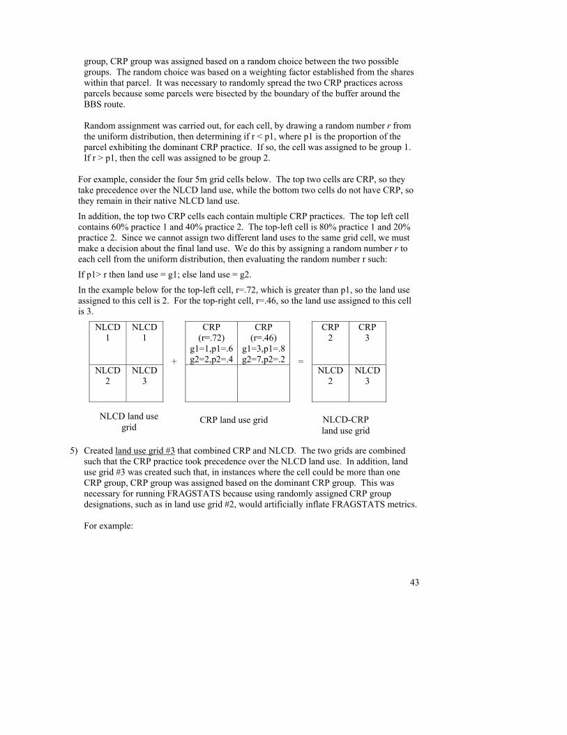
43
group, CRP group was assigned based on a random choice between the two possible groups. The random choice was based on a weighting factor established from the shares within that parcel. It was necessary to randomly spread the two CRP practices across parcels because some parcels were bisected by the boundary of the buffer around the BBS route. Random assignment was carried out, for each cell, by drawing a random number r from the uniform distribution, then determining if r < p1, where p1 is the proportion of the parcel exhibiting the dominant CRP practice. If so, the cell was assigned to be group 1. If r > p1, then the cell was assigned to be group 2.
For example, consider the four 5m grid cells below. The top two cells are CRP, so they take precedence over the NLCD land use, while the bottom two cells do not have CRP, so they remain in their native NLCD land use.
In addition, the top two CRP cells each contain multiple CRP practices. The top left cell contains 60% practice 1 and 40% practice 2. The top-left cell is 80% practice 1 and 20% practice 2. Since we cannot assign two different land uses to the same grid cell, we must make a decision about the final land use. We do this by assigning a random number r to each cell from the uniform distribution, then evaluating the random number r such:
If p1> r then land use = g1; else land use = g2.
In the example below for the top-left cell, r=.72, which is greater than p1, so the land use assigned to this cell is 2. For the top-right cell, r=.46, so the land use assigned to this cell is 3.
NLCD 1
NLCD 1
CRP (r=.72)
g1=1,p1=.6g2=2,p2=.4
CRP (r=.46)
g1=3,p1=.8g2=7,p2=.2
CRP 2
CRP 3
NLCD 2
NLCD 3
+
= NLCD
2 NLCD
3
5) Created land use grid #3 that combined CRP and NLCD. The two grids are combined such that the CRP practice took precedence over the NLCD land use. In addition, land use grid #3 was created such that, in instances where the cell could be more than one CRP group, CRP group was assigned based on the dominant CRP group. This was necessary for running FRAGSTATS because using randomly assigned CRP group designations, such as in land use grid #2, would artificially inflate FRAGSTATS metrics.
For example:
NLCD land use grid
CRP land use grid NLCD-CRP land use grid
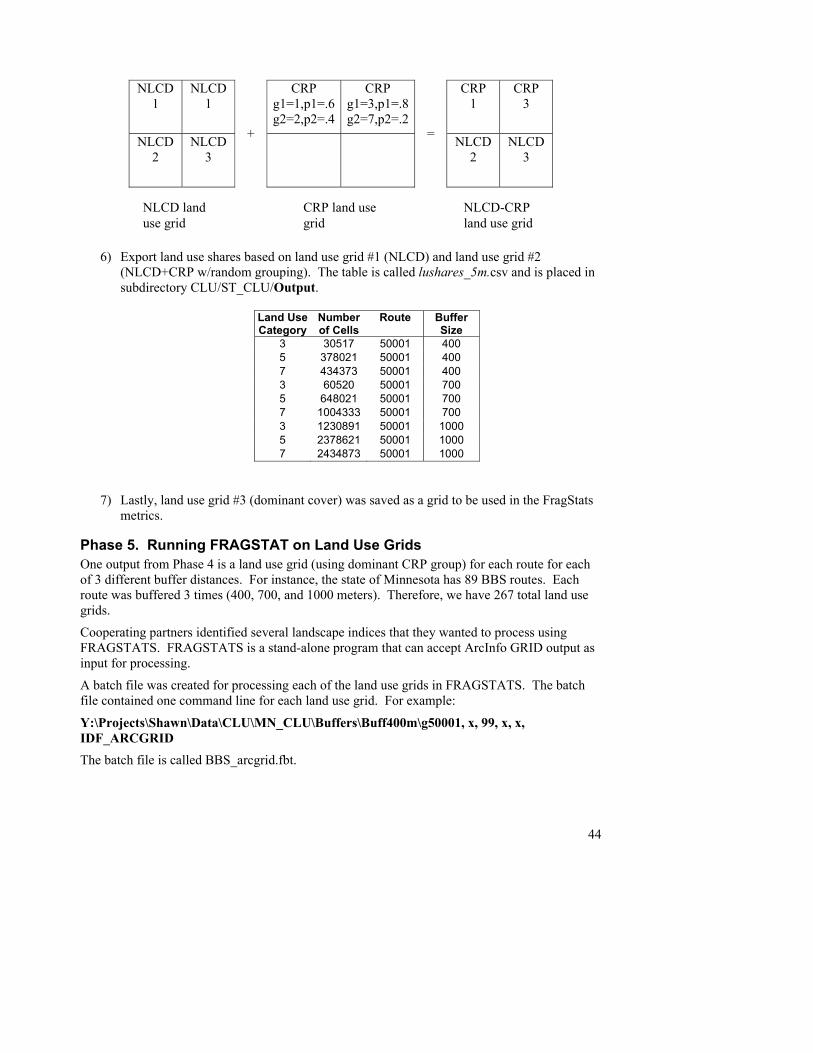
44
NLCD 1
NLCD 1
CRP g1=1,p1=.6g2=2,p2=.4
CRP g1=3,p1=.8g2=7,p2=.2
CRP 1
CRP 3
NLCD 2
NLCD 3
+ = NLCD2
NLCD3
6) Export land use shares based on land use grid #1 (NLCD) and land use grid #2
(NLCD+CRP w/random grouping). The table is called lushares_5m.csv and is placed in subdirectory CLU/ST_CLU/Output.
Land Use Category
Number of Cells
Route Buffer Size
3 30517 50001 400 5 378021 50001 400 7 434373 50001 400 3 60520 50001 700 5 648021 50001 700 7 1004333 50001 700 3 1230891 50001 1000 5 2378621 50001 1000 7 2434873 50001 1000
7) Lastly, land use grid #3 (dominant cover) was saved as a grid to be used in the FragStats
metrics.
Phase 5. Running FRAGSTAT on Land Use Grids One output from Phase 4 is a land use grid (using dominant CRP group) for each route for each of 3 different buffer distances. For instance, the state of Minnesota has 89 BBS routes. Each route was buffered 3 times (400, 700, and 1000 meters). Therefore, we have 267 total land use grids.
Cooperating partners identified several landscape indices that they wanted to process using FRAGSTATS. FRAGSTATS is a stand-alone program that can accept ArcInfo GRID output as input for processing.
A batch file was created for processing each of the land use grids in FRAGSTATS. The batch file contained one command line for each land use grid. For example:
Y:\Projects\Shawn\Data\CLU\MN_CLU\Buffers\Buff400m\g50001, x, 99, x, x, IDF_ARCGRID The batch file is called BBS_arcgrid.fbt.
NLCD land use grid
CRP land use grid
NLCD-CRP land use grid
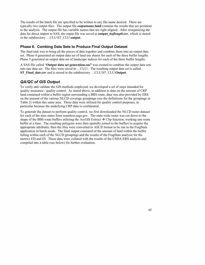
45
The results of the batch file are specified to be written to any file name desired. There are typically two output files. The output file outputname.land contains the results that are pertinent to the analysis. The output file has variable names that are right aligned. After reorganizing the data for direct import to SAS, the ouput file was saved as output_buflength.csv, which is stored in the subdirectory …CLU\ST_CLU\output.
Phase 6. Combing Data Sets to Produce Final Output Dataset The final task was to bring all the pieces of data together and combine them into an output data set. Phase 4 generated an output data set of land use shares for each of the three buffer lengths. Phase 5 generated an output data set of landscape indices for each of the three buffer lengths.
A SAS file called “Output data set generation.sas” was created to combine the output data sets into one data set. The files were saved in …CLU\. The resulting output data set is called ST_Final_date.csv and is stored in the subdirectory …CLU\ST_CLU\Output.
QA/QC of GIS Output To verify and validate the GIS methods employed, we developed a set of steps intended for quality assurance / quality control. As stated above, in addition to data on the amount of CRP land contained within a buffer region surrounding a BBS route, data was also provided by ERS on the amount of the various NLCD coverage groupings (see the definitions for the groupings in Table 2) within this same area. These data were utilized for quality control purposes, in particular because the underlying CRP data is confidential.
To generate the dataset to perform quality control, we first downloaded the NLCD raster dataset for each of the nine states from seamless.usgs.gov. The state-wide raster was cut down to the shape of the BBS route buffers utilizing the ArcGIS Extract Clip function, working one route buffer at a time. The resulting polygons were then spatially joined to the buffers to acquire the appropriate attributes, then the files were converted to ASCII format to be run in the FragStats application in batch mode. The final output consisted of the amount of land within the buffer falling within each of the NLCD groupings and the results of the FragStats analysis for the metrics ED and IJI. These data were collated with the results of the USDA-ERS analysis and compiled into a table (see below) for further evaluation.
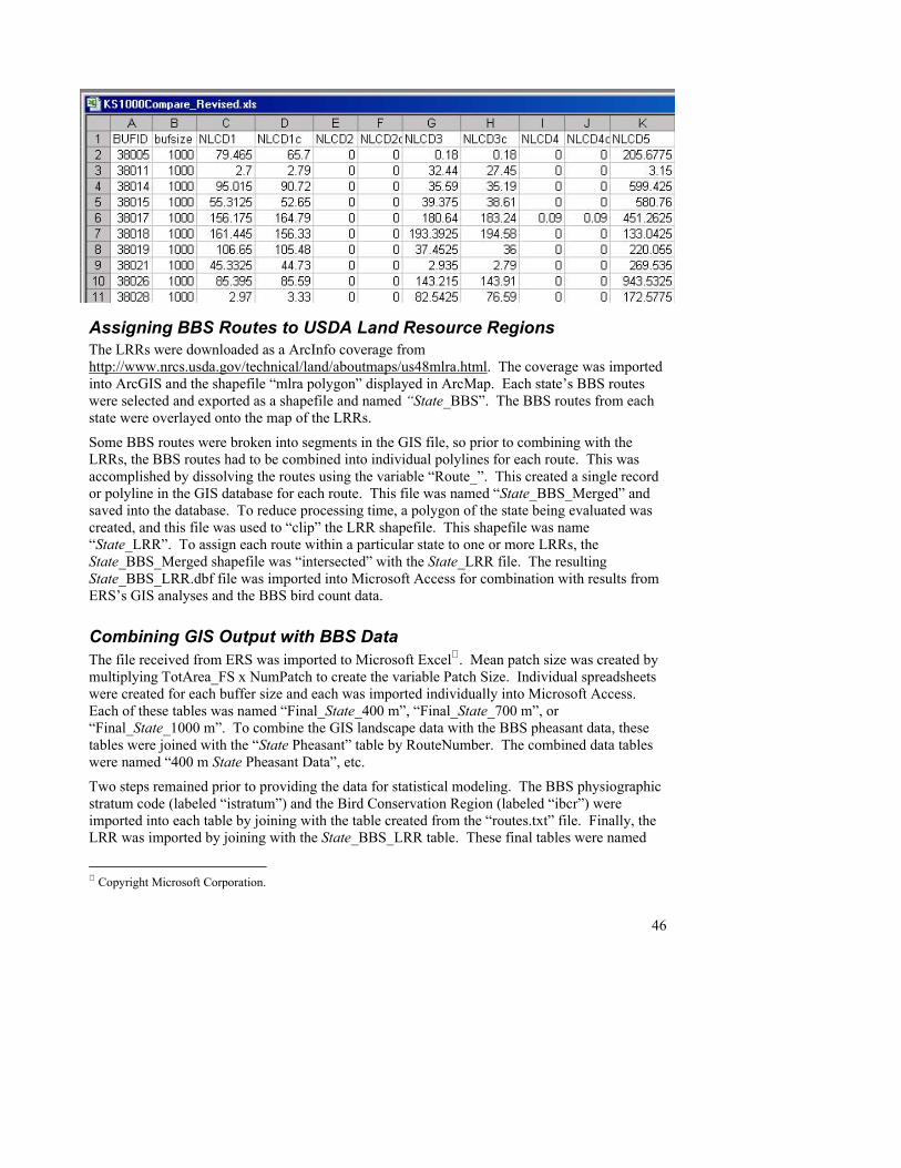
46
Assigning BBS Routes to USDA Land Resource Regions The LRRs were downloaded as a ArcInfo coverage from http://www.nrcs.usda.gov/technical/land/aboutmaps/us48mlra.html. The coverage was imported into ArcGIS and the shapefile “mlra polygon” displayed in ArcMap. Each state’s BBS routes were selected and exported as a shapefile and named “State_BBS”. The BBS routes from each state were overlayed onto the map of the LRRs.
Some BBS routes were broken into segments in the GIS file, so prior to combining with the LRRs, the BBS routes had to be combined into individual polylines for each route. This was accomplished by dissolving the routes using the variable “Route_”. This created a single record or polyline in the GIS database for each route. This file was named “State_BBS_Merged” and saved into the database. To reduce processing time, a polygon of the state being evaluated was created, and this file was used to “clip” the LRR shapefile. This shapefile was name “State_LRR”. To assign each route within a particular state to one or more LRRs, the State_BBS_Merged shapefile was “intersected” with the State_LRR file. The resulting State_BBS_LRR.dbf file was imported into Microsoft Access for combination with results from ERS’s GIS analyses and the BBS bird count data.
Combining GIS Output with BBS Data The file received from ERS was imported to Microsoft Excel . Mean patch size was created by multiplying TotArea_FS x NumPatch to create the variable Patch Size. Individual spreadsheets were created for each buffer size and each was imported individually into Microsoft Access. Each of these tables was named “Final_State_400 m”, “Final_State_700 m”, or “Final_State_1000 m”. To combine the GIS landscape data with the BBS pheasant data, these tables were joined with the “State Pheasant” table by RouteNumber. The combined data tables were named “400 m State Pheasant Data”, etc.
Two steps remained prior to providing the data for statistical modeling. The BBS physiographic stratum code (labeled “istratum”) and the Bird Conservation Region (labeled “ibcr”) were imported into each table by joining with the table created from the “routes.txt” file. Finally, the LRR was imported by joining with the State_BBS_LRR table. These final tables were named
Copyright Microsoft Corporation.

47
“400 m State Pheasant_LRR”, etc. These tables were exported from Access as comma delimited files for use in SAS.
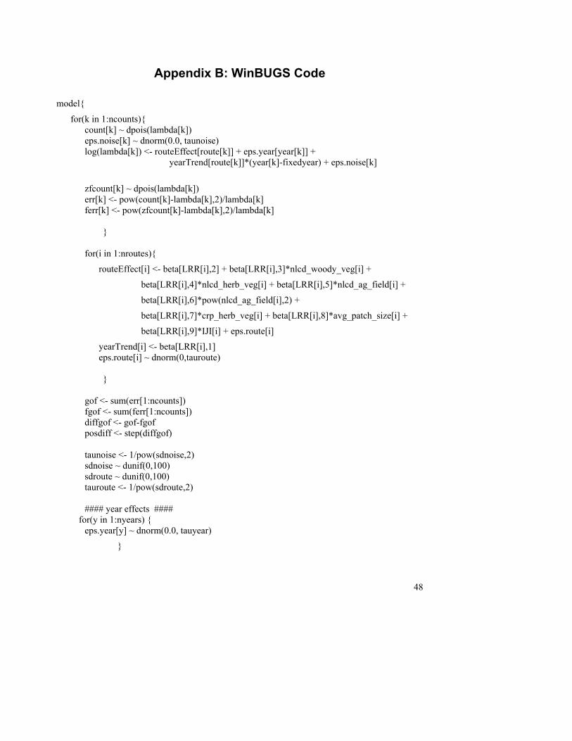
48
Appendix B: WinBUGS Code
model{
for(k in 1:ncounts){ count[k] ~ dpois(lambda[k]) eps.noise[k] ~ dnorm(0.0, taunoise) log(lambda[k]) <- routeEffect[route[k]] + eps.year[year[k]] +
yearTrend[route[k]]*(year[k]-fixedyear) + eps.noise[k]
zfcount[k] ~ dpois(lambda[k]) err[k] <- pow(count[k]-lambda[k],2)/lambda[k] ferr[k] <- pow(zfcount[k]-lambda[k],2)/lambda[k] }
for(i in 1:nroutes){
routeEffect[i] <- beta[LRR[i],2] + beta[LRR[i],3]*nlcd_woody_veg[i] +
beta[LRR[i],4]*nlcd_herb_veg[i] + beta[LRR[i],5]*nlcd_ag_field[i] +
beta[LRR[i],6]*pow(nlcd_ag_field[i],2) +
beta[LRR[i],7]*crp_herb_veg[i] + beta[LRR[i],8]*avg_patch_size[i] +
beta[LRR[i],9]*IJI[i] + eps.route[i]
yearTrend[i] <- beta[LRR[i],1] eps.route[i] ~ dnorm(0,tauroute)
}
gof <- sum(err[1:ncounts]) fgof <- sum(ferr[1:ncounts]) diffgof <- gof-fgof posdiff <- step(diffgof)
taunoise <- 1/pow(sdnoise,2) sdnoise ~ dunif(0,100) sdroute ~ dunif(0,100) tauroute <- 1/pow(sdroute,2) #### year effects ####
for(y in 1:nyears) { eps.year[y] ~ dnorm(0.0, tauyear)
}
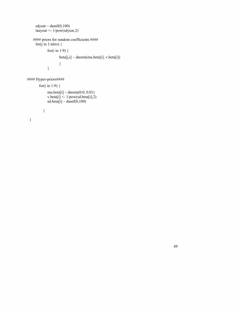
49
sdyear ~ dunif(0,100) tauyear <- 1/pow(sdyear,2)
#### priors for random coefficients ####
for(j in 1:nlrrs) {
for(i in 1:9) {
beta[j,i] ~ dnorm(mu.beta[i], v.beta[i])
} }
#### Hyper-priors####
for(i in 1:9) {
mu.beta[i] ~ dnorm(0.0, 0.01) v.beta[i] <- 1/pow(sd.beta[i],2) sd.beta[i] ~ dunif(0,100)
} }

50
Appendix C: CAR Model Overall, route effects were modeled as a multivariate normal
( )1 388, , ~ ( , )CARNω ω ω= 0 ΣK . [1]
The CAR model is defined by all of the conditional distributions
( )2| ~ ,i i i iNω µ τ−ω , [2]
where,
i
i ij jj n
cµ φ ω∈
= ∑ [3]
and in is the collection of neighbors for the ith BBS route. The weights ijc satisfy the constraint 2 2
ij j ji ic cτ τ= and ijc = 0 if the jth unit is not a neighbor of the ith unit.
The conditional distributions define the covariance matrix 1( )CAR φ −= −Σ I C M , [4]
where C is an n n× matrix with elements ijc and M is a diagonal matrix with elements 2iτ . If
0φ = , then the CAR model reduces to an independent effects model. We used
{ }0, > 430
max , <=430 ij
ij k kij ij ij
dc
d d d− −
=
, [5]
with k = 1, and 2 2 / | |i inτ τ= , [6]
which gives 2 1( )CAR Dτ φ −= −Σ I C , [7]
where D is a diagonal matrix with elements equal to number of neighbors ( | |in ). The distance weighted CAR model allows spatial association that decreases with distance. This is similar to a geostatistical spatial process, but is much less computationally expensive.
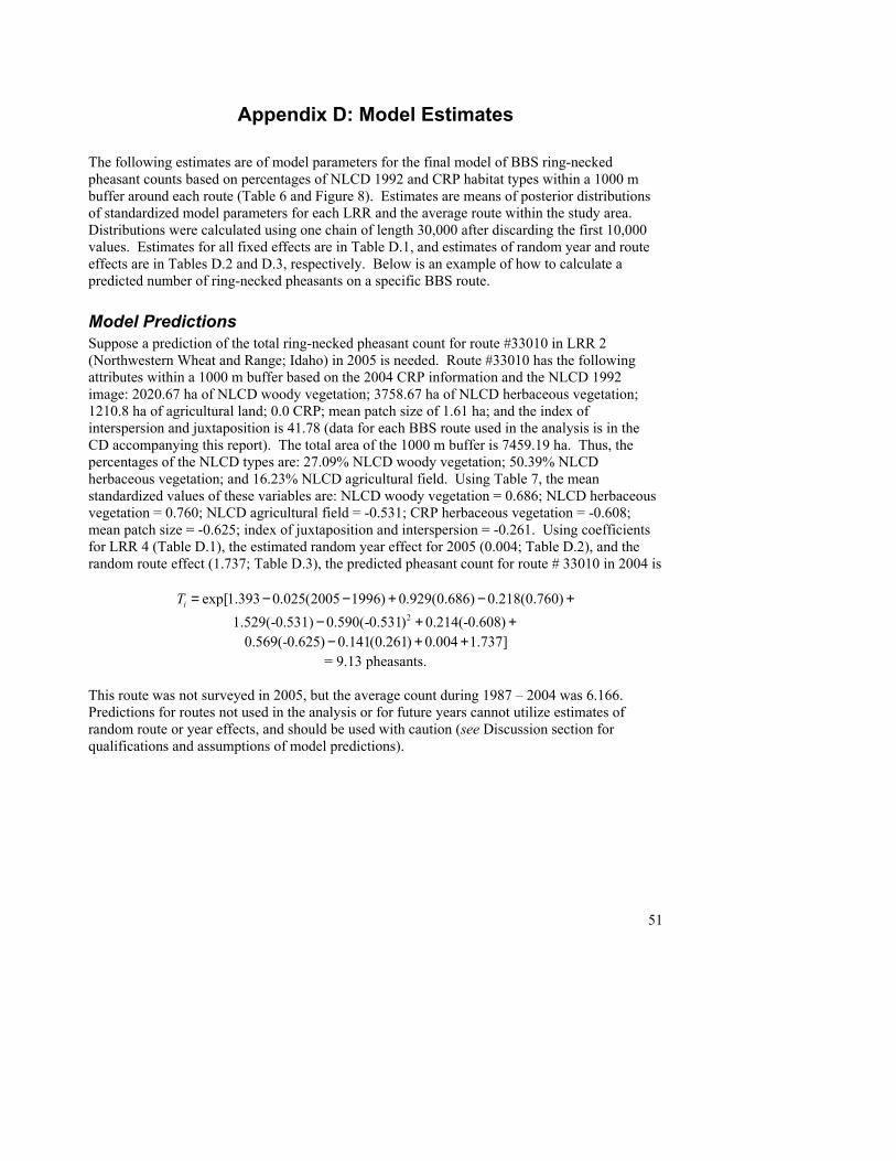
51
Appendix D: Model Estimates
The following estimates are of model parameters for the final model of BBS ring-necked pheasant counts based on percentages of NLCD 1992 and CRP habitat types within a 1000 m buffer around each route (Table 6 and Figure 8). Estimates are means of posterior distributions of standardized model parameters for each LRR and the average route within the study area. Distributions were calculated using one chain of length 30,000 after discarding the first 10,000 values. Estimates for all fixed effects are in Table D.1, and estimates of random year and route effects are in Tables D.2 and D.3, respectively. Below is an example of how to calculate a predicted number of ring-necked pheasants on a specific BBS route.
Model Predictions Suppose a prediction of the total ring-necked pheasant count for route #33010 in LRR 2 (Northwestern Wheat and Range; Idaho) in 2005 is needed. Route #33010 has the following attributes within a 1000 m buffer based on the 2004 CRP information and the NLCD 1992 image: 2020.67 ha of NLCD woody vegetation; 3758.67 ha of NLCD herbaceous vegetation; 1210.8 ha of agricultural land; 0.0 CRP; mean patch size of 1.61 ha; and the index of interspersion and juxtaposition is 41.78 (data for each BBS route used in the analysis is in the CD accompanying this report). The total area of the 1000 m buffer is 7459.19 ha. Thus, the percentages of the NLCD types are: 27.09% NLCD woody vegetation; 50.39% NLCD herbaceous vegetation; and 16.23% NLCD agricultural field. Using Table 7, the mean standardized values of these variables are: NLCD woody vegetation = 0.686; NLCD herbaceous vegetation = 0.760; NLCD agricultural field = -0.531; CRP herbaceous vegetation = -0.608; mean patch size = -0.625; index of juxtaposition and interspersion = -0.261. Using coefficients for LRR 4 (Table D.1), the estimated random year effect for 2005 (0.004; Table D.2), and the random route effect (1.737; Table D.3), the predicted pheasant count for route # 33010 in 2004 is
exp[1.393 0.025(2005 1996) 0.929(0.686) 0.218(0.760)iT = − − + − + 21.529(-0.531) 0.590(-0.531) 0.214(-0.608)− + +
0.569(-0.625) 0.141(0.261) 0.004 1.737]− + + = 9.13 pheasants.
This route was not surveyed in 2005, but the average count during 1987 – 2004 was 6.166. Predictions for routes not used in the analysis or for future years cannot utilize estimates of random route or year effects, and should be used with caution (see Discussion section for qualifications and assumptions of model predictions).
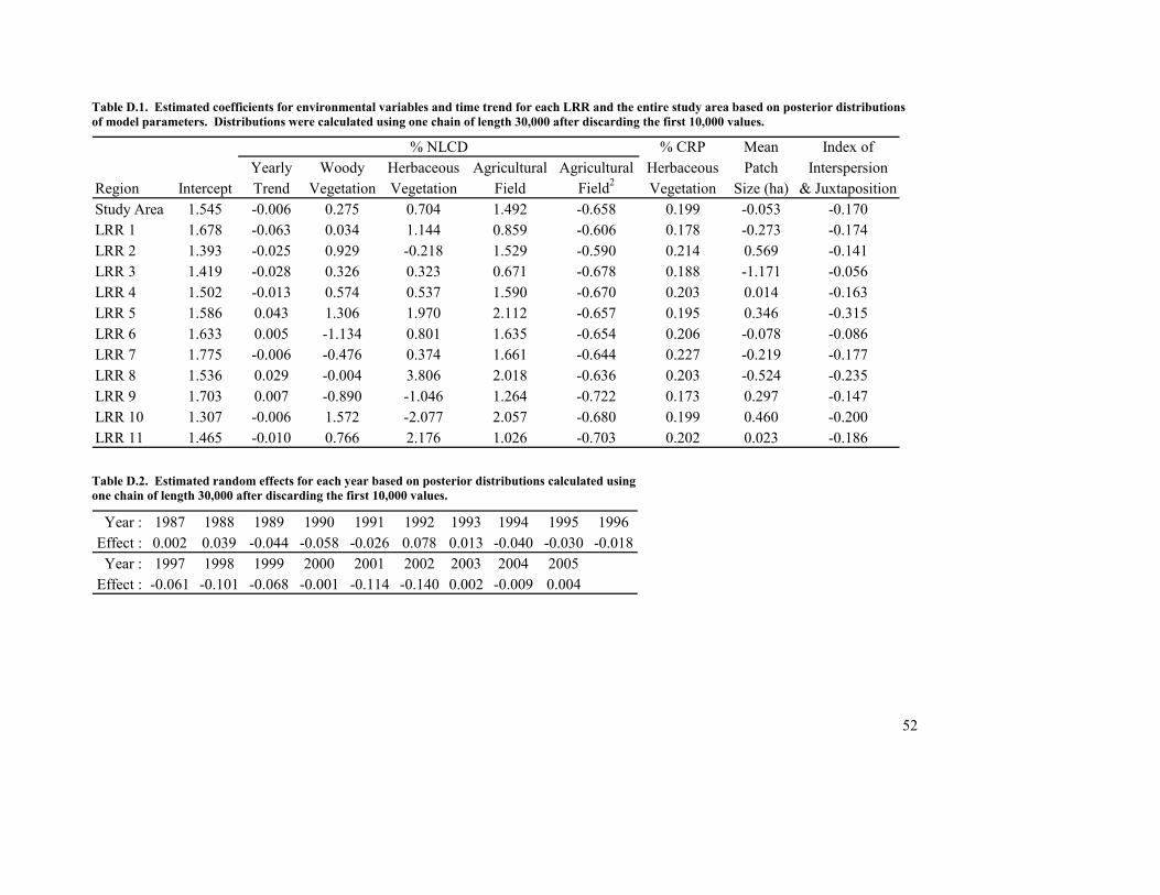
52
Table D.1. Estimated coefficients for environmental variables and time trend for each LRR and the entire study area based on posterior distributions of model parameters. Distributions were calculated using one chain of length 30,000 after discarding the first 10,000 values.
% CRP Mean Index ofYearly Woody Herbaceous Agricultural Agricultural Herbaceous Patch Interspersion
Region Intercept Trend Vegetation Vegetation Field Field2 Vegetation Size (ha) & JuxtapositionStudy Area 1.545 -0.006 0.275 0.704 1.492 -0.658 0.199 -0.053 -0.170LRR 1 1.678 -0.063 0.034 1.144 0.859 -0.606 0.178 -0.273 -0.174LRR 2 1.393 -0.025 0.929 -0.218 1.529 -0.590 0.214 0.569 -0.141LRR 3 1.419 -0.028 0.326 0.323 0.671 -0.678 0.188 -1.171 -0.056LRR 4 1.502 -0.013 0.574 0.537 1.590 -0.670 0.203 0.014 -0.163LRR 5 1.586 0.043 1.306 1.970 2.112 -0.657 0.195 0.346 -0.315LRR 6 1.633 0.005 -1.134 0.801 1.635 -0.654 0.206 -0.078 -0.086LRR 7 1.775 -0.006 -0.476 0.374 1.661 -0.644 0.227 -0.219 -0.177LRR 8 1.536 0.029 -0.004 3.806 2.018 -0.636 0.203 -0.524 -0.235LRR 9 1.703 0.007 -0.890 -1.046 1.264 -0.722 0.173 0.297 -0.147LRR 10 1.307 -0.006 1.572 -2.077 2.057 -0.680 0.199 0.460 -0.200LRR 11 1.465 -0.010 0.766 2.176 1.026 -0.703 0.202 0.023 -0.186
% NLCD
Table D.2. Estimated random effects for each year based on posterior distributions calculated using one chain of length 30,000 after discarding the first 10,000 values.
Year : 1987 1988 1989 1990 1991 1992 1993 1994 1995 1996Effect : 0.002 0.039 -0.044 -0.058 -0.026 0.078 0.013 -0.040 -0.030 -0.018
Year : 1997 1998 1999 2000 2001 2002 2003 2004 2005Effect : -0.061 -0.101 -0.068 -0.001 -0.114 -0.140 0.002 -0.009 0.004
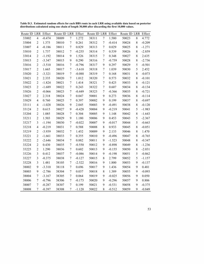
53
Table D.3. Estimated random effects for each BBS route in each LRR using available data based on posterior distributions calculated using one chain of length 30,000 after discarding the first 10,000 values.
Route ID LRR Effect Route ID LRR Effect Route ID LRR Effect Route ID LRR Effect33002 4 -0.474 38009 7 1.272 38311 7 1.580 50023 8 4.77233004 2 1.375 38010 7 0.261 38312 7 -0.414 50024 8 -0.20933007 4 -0.186 38011 7 0.829 38313 7 0.029 50025 8 -1.27133010 2 1.737 38012 7 -0.255 38314 7 0.539 50026 8 -2.85933014 2 -1.192 38014 9 1.526 38315 7 0.348 50027 8 2.63533015 2 -3.347 38015 9 0.290 38316 7 -0.759 50028 8 -2.73633016 2 -3.510 38016 7 -0.796 38317 9 0.297 50029 5 -0.50133017 2 1.665 38017 7 -3.610 38318 7 1.039 50030 5 2.45233020 2 -3.321 38019 7 -0.088 38319 7 0.168 50031 8 -0.07333021 2 2.335 38020 7 1.012 38320 7 0.573 50032 8 -0.10133022 2 -1.824 38021 7 1.414 38321 7 0.425 50033 8 -0.12133023 2 -1.689 38022 7 0.243 38322 7 0.607 50034 8 -0.13433026 2 -0.066 38023 7 -0.449 38323 7 -0.366 50035 8 -0.72133027 2 2.318 38024 7 0.047 50001 9 0.273 50036 8 -0.11433029 4 0.760 38025 7 0.397 50002 9 0.199 50037 8 -0.69733111 4 -1.028 38026 9 2.045 50003 9 -0.491 50038 8 -0.12033124 2 0.615 38027 9 -0.428 50004 9 -0.219 50041 5 -1.98333204 2 1.085 38028 7 0.304 50005 9 1.148 50042 8 -1.64333211 2 1.503 38029 9 1.180 50006 9 0.453 50043 5 -2.36733217 3 -1.194 38030 7 -0.022 50007 9 -0.017 50044 5 -0.66333218 4 -0.219 38031 7 0.588 50008 8 0.933 50045 8 -0.05133219 2 -3.939 38032 7 1.452 50009 9 2.133 50046 8 1.47033221 2 -1.661 38033 7 0.355 50010 9 -0.496 50047 8 -0.76533222 2 -2.646 38034 7 0.882 50011 9 -1.523 50048 8 -0.34733224 2 0.430 38035 7 -0.550 50012 9 -0.898 50049 8 -1.23633225 2 1.290 38036 7 0.602 50013 9 -0.155 50050 8 -2.03133226 3 0.412 38037 7 -0.086 50014 9 -0.198 50051 5 -0.86233227 3 -0.375 38038 7 -0.127 50015 8 2.799 50052 5 -1.15733228 3 1.481 38105 7 -2.522 50016 9 1.800 50053 9 -0.13738002 9 -3.310 38118 7 0.696 50017 9 1.436 50054 9 0.48138003 9 -2.786 38304 7 0.037 50018 8 1.389 50055 9 -0.09338004 7 -3.167 38305 7 0.064 50019 9 -0.025 50056 9 0.05038006 7 -0.796 38306 7 -0.173 50020 9 -0.296 50057 9 0.80638007 7 -0.287 38307 7 0.199 50021 9 -0.531 50058 9 -0.37538008 7 -0.397 38308 7 -1.120 50022 8 -0.512 50059 9 -0.849
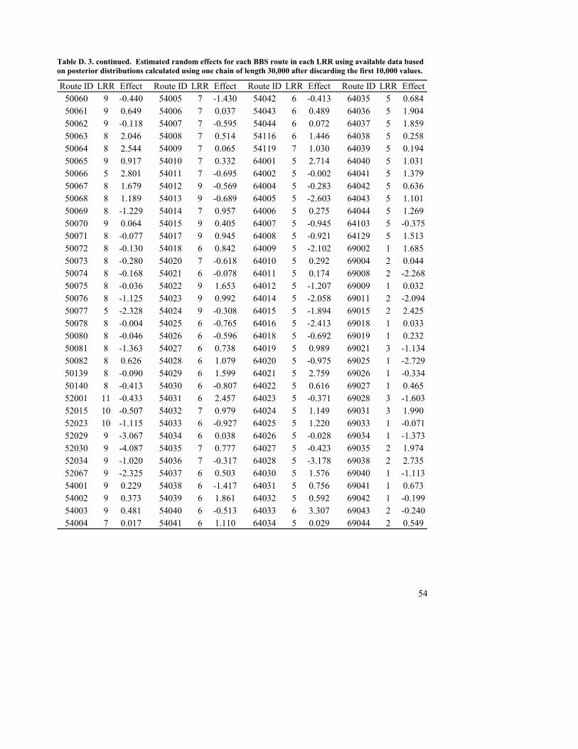
54
Table D. 3. continued. Estimated random effects for each BBS route in each LRR using available data based on posterior distributions calculated using one chain of length 30,000 after discarding the first 10,000 values.
Route ID LRR Effect Route ID LRR Effect Route ID LRR Effect Route ID LRR Effect50060 9 -0.440 54005 7 -1.430 54042 6 -0.413 64035 5 0.68450061 9 0.649 54006 7 0.037 54043 6 0.489 64036 5 1.90450062 9 -0.118 54007 7 -0.595 54044 6 0.072 64037 5 1.85950063 8 2.046 54008 7 0.514 54116 6 1.446 64038 5 0.25850064 8 2.544 54009 7 0.065 54119 7 1.030 64039 5 0.19450065 9 0.917 54010 7 0.332 64001 5 2.714 64040 5 1.03150066 5 2.801 54011 7 -0.695 64002 5 -0.002 64041 5 1.37950067 8 1.679 54012 9 -0.569 64004 5 -0.283 64042 5 0.63650068 8 1.189 54013 9 -0.689 64005 5 -2.603 64043 5 1.10150069 8 -1.229 54014 7 0.957 64006 5 0.275 64044 5 1.26950070 9 0.064 54015 9 0.405 64007 5 -0.945 64103 5 -0.37550071 8 -0.077 54017 9 0.945 64008 5 -0.921 64129 5 1.51350072 8 -0.130 54018 6 0.842 64009 5 -2.102 69002 1 1.68550073 8 -0.280 54020 7 -0.618 64010 5 0.292 69004 2 0.04450074 8 -0.168 54021 6 -0.078 64011 5 0.174 69008 2 -2.26850075 8 -0.036 54022 9 1.653 64012 5 -1.207 69009 1 0.03250076 8 -1.125 54023 9 0.992 64014 5 -2.058 69011 2 -2.09450077 5 -2.328 54024 9 -0.308 64015 5 -1.894 69015 2 2.42550078 8 -0.004 54025 6 -0.765 64016 5 -2.413 69018 1 0.03350080 8 -0.046 54026 6 -0.596 64018 5 -0.692 69019 1 0.23250081 8 -1.363 54027 6 0.738 64019 5 0.989 69021 3 -1.13450082 8 0.626 54028 6 1.079 64020 5 -0.975 69025 1 -2.72950139 8 -0.090 54029 6 1.599 64021 5 2.759 69026 1 -0.33450140 8 -0.413 54030 6 -0.807 64022 5 0.616 69027 1 0.46552001 11 -0.433 54031 6 2.457 64023 5 -0.371 69028 3 -1.60352015 10 -0.507 54032 7 0.979 64024 5 1.149 69031 3 1.99052023 10 -1.115 54033 6 -0.927 64025 5 1.220 69033 1 -0.07152029 9 -3.067 54034 6 0.038 64026 5 -0.028 69034 1 -1.37352030 9 -4.087 54035 7 0.777 64027 5 -0.423 69035 2 1.97452034 9 -1.020 54036 7 -0.317 64028 5 -3.178 69038 2 2.73552067 9 -2.325 54037 6 0.503 64030 5 1.576 69040 1 -1.11354001 9 0.229 54038 6 -1.417 64031 5 0.756 69041 1 0.67354002 9 0.373 54039 6 1.861 64032 5 0.592 69042 1 -0.19954003 9 0.481 54040 6 -0.513 64033 6 3.307 69043 2 -0.24054004 7 0.017 54041 6 1.110 64034 5 0.029 69044 2 0.549
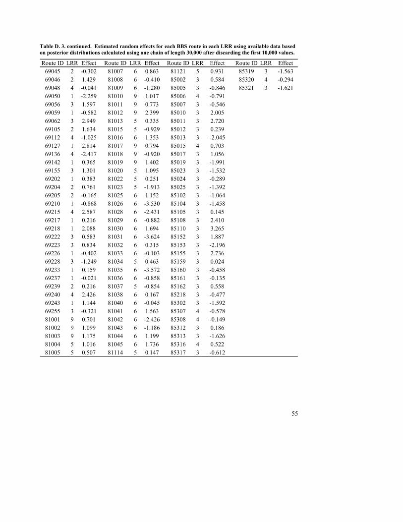
55
Table D. 3. continued. Estimated random effects for each BBS route in each LRR using available data based on posterior distributions calculated using one chain of length 30,000 after discarding the first 10,000 values.
Route ID LRR Effect Route ID LRR Effect Route ID LRR Effect Route ID LRR Effect69045 2 -0.302 81007 6 0.863 81121 5 0.931 85319 3 -1.56369046 2 1.429 81008 6 -0.410 85002 3 0.584 85320 4 -0.29469048 4 -0.041 81009 6 -1.280 85005 3 -0.846 85321 3 -1.62169050 1 -2.259 81010 9 1.017 85006 4 -0.79169056 3 1.597 81011 9 0.773 85007 3 -0.54669059 1 -0.582 81012 9 2.399 85010 3 2.00569062 3 2.949 81013 5 0.335 85011 3 2.72069105 2 1.634 81015 5 -0.929 85012 3 0.23969112 4 -1.025 81016 6 1.353 85013 3 -2.04569127 1 2.814 81017 9 0.794 85015 4 0.70369136 4 -2.417 81018 9 -0.920 85017 3 1.05669142 1 0.365 81019 9 1.402 85019 3 -1.99169155 3 1.301 81020 5 1.095 85023 3 -1.53269202 1 0.383 81022 5 0.251 85024 3 -0.28969204 2 0.761 81023 5 -1.913 85025 3 -1.39269205 2 -0.165 81025 6 1.152 85102 3 -1.06469210 1 -0.868 81026 6 -3.530 85104 3 -1.45869215 4 2.587 81028 6 -2.431 85105 3 0.14569217 1 0.216 81029 6 -0.882 85108 3 2.41069218 1 2.088 81030 6 1.694 85110 3 3.26569222 3 0.583 81031 6 -3.624 85152 3 1.88769223 3 0.834 81032 6 0.315 85153 3 -2.19669226 1 -0.402 81033 6 -0.103 85155 3 2.73669228 3 -1.249 81034 5 0.463 85159 3 0.02469233 1 0.159 81035 6 -3.572 85160 3 -0.45869237 1 -0.021 81036 6 -0.858 85161 3 -0.13569239 2 0.216 81037 5 -0.854 85162 3 0.55869240 4 2.426 81038 6 0.167 85218 3 -0.47769243 1 1.144 81040 6 -0.045 85302 3 -1.59269255 3 -0.321 81041 6 1.563 85307 4 -0.57881001 9 0.701 81042 6 -2.426 85308 4 -0.14981002 9 1.099 81043 6 -1.186 85312 3 0.18681003 9 1.175 81044 6 1.199 85313 3 -1.62681004 5 1.016 81045 6 1.736 85316 4 0.52281005 5 0.507 81114 5 0.147 85317 3 -0.612