ESTIMATING REQUIRED CONTINGENCY FUNDS FOR

CONSTRUCTION PROJECTS USING MULTPLE LINEAR REGRESSION

THESIS

Jason J. Cook, Captain, USAF

AFIT/GEM/ENV/06M-02

DEPARTMENT OF THE AIR FORCE AIR UNIVERSITY

AIR FORCE INSTITUTE OF TECHNOLOGY

Wright-Patterson Air Force Base, Ohio

APPROVED FOR PUBLIC RELEASE; DISTRIBUTION UNLIMITED

The views expressed in this thesis are those of the author and do not reflect the official policy or position of the United States Air Force, Department of Defense, or the United States Government.

AFIT/GEM/ENV/06M-02

ESTIMATING REQUIRED CONTINGENCY FUNDS FOR CONSTRUCTION PROJECTS USING MULTPLE LINEAR REGRESSION

THESIS

Presented to the Faculty

Department of Systems and Engineering Management

Graduate School of Engineering and Management

Air Force Institute of Technology

Air University

Air Education and Training Command

In Partial Fulfillment of the Requirements for the

Degree of Master of Science in Engineering Management

Jason J. Cook, BS

Captain, USAF

March 2006

APPROVED FOR PUBLIC RELEASE; DISTRIBUTION UNLIMITED.

AFIT/GEM/ENV/06M-02

ESTIMATING REQUIRED CONTINGENCY FUNDS FOR CONSTRUCTION PROJECTS USING MULTPLE LINEAR REGRESSION

Jason J. Cook, BS Captain, USAF

Approved: /signed/ 17 Mar 06 ______________________________________ __________ Alfred E. Thal, Jr., PhD (Chairman) date /signed/ 16 Mar 06 ______________________________________ __________ Jared A. Astin, Colonel, USAF (Member) date /signed/ 15 Mar 06 ______________________________________ __________ Edward D. White III, PhD (Member) date

iv

AFIT/GEM/ENV/06M-02

Abstract

Cost overruns are a critical problem for construction projects. The common

practice for dealing with cost overruns is the assignment of an arbitrary flat percentage of

the construction budget as a contingency fund. This research seeks to identify significant

factors that may influence, or serve as indicators of, potential cost overruns. The study

uses data on 243 construction projects over a full range of project types and scopes

gathered from an existing United States Air Force construction database. The author uses

multiple linear regression to analyze the data and compares the proposed model to the

common practice of assigning contingency funds. The multiple linear regression model

provides better predictions of actual cost overruns experienced. Based on the

performance metric used, the model sufficiently captures 44% of actual cost overruns

versus current practices capturing only 20%

The proposed model developed in this study only uses data that would be

available prior to the award of a construction contract. This allows the model to serve as

a planning tool throughout the concept and design phases. The model includes project

characteristics, design performance metrics, and contract award process influences. This

research supports prior findings of a relationship between design funding and design

performance as well as the influence of the contract award process on cost overruns.

While the proposed model captures 44% of actual cost overruns, its application reduces

average contingency budgeting error from -11.2% to only -0.3% over the entire test

sample.

v

Acknowledgments

First, I would like to acknowledge the influence and help of Greg Hoffman. His

work served as the inspiration for this study, and his help early in the process proved

critical to its success. I would like to thank my thesis advisor, Dr. Al Thal, for his endless

patience and invaluable insights that greatly improved the quality of this effort. I would

also thank my committee members, Col Jared Astin and Dr. Edward White, for all of

their advice and support. Tyler Nielsen, thank you for acting as a sounding board for my

ideas and helping to put things in perspective. Finally, and of course most importantly, I

could not have done this work without the love, support, and understanding of my wife.

Jason J. Cook

vi

Table of Contents

Page Abstract.............................................................................................................................. iv

Acknowledgments ...............................................................................................................v

Table of Contents............................................................................................................... vi

List of Figures.................................................................................................................. viii

List of Tables ..................................................................................................................... ix

I. Introduction .....................................................................................................................1

General Background ........................................................................................................1 Specific Background........................................................................................................5 Research Question ...........................................................................................................6 Investigative Questions....................................................................................................7 Proposed Methodology....................................................................................................7 Limitations.......................................................................................................................8

II. Literature Review...........................................................................................................9

Existing Models ...............................................................................................................9

Artificial Neural Network (ANN)............................................................................... 9 Multiple Linear Regression....................................................................................... 12

Causes of Construction Cost Overruns..........................................................................14 Conclusion .....................................................................................................................17

III. Methodology...............................................................................................................18

Step 1: Hypothesize the Deterministic Component of the Model ................................18 Step 2: Estimate Model Parameters ..............................................................................20 Step 3: Specify the Probability Distribution of the Random Error Term .....................21 Step 4: Check Assumptions of the Random Error Term ..............................................21 Step 5: Statistically Evaluate the Usefulness of the Model ..........................................24 Step 6: Use the Model for Prediction ...........................................................................26 Conclusion .....................................................................................................................27

IV. Results ........................................................................................................................28

Data Collection ..............................................................................................................28

vii

Page

Identification of Candidate Independent Variables .......................................................29 Iterative Process of Modeling........................................................................................31 Proposed Model .............................................................................................................32 Test the Proposed Model against Methodology Assumptions ......................................33 Statistically Evaluate the Usefulness of the Model .......................................................36 Use the Model for Prediction.........................................................................................38 Conclusion .....................................................................................................................40

V. Conclusions..................................................................................................................41

Discussion of Results.....................................................................................................41 Limitations.....................................................................................................................45 Recommendations..........................................................................................................46

Usefulness of the Model ........................................................................................... 46 Future Research ........................................................................................................ 47

Appendix: JMP® Regression Model Output ....................................................................49

References..........................................................................................................................54

viii

List of Figures

Figure Page 1. Plot of Model Predicted Values vs. Residuals ............................................................. 33 2. Histogram of Studentized Residuals with a Fitted Normal Distribution ..................... 35 3. Histogram of Cook's Distance ..................................................................................... 35

ix

List of Tables

Table Page 1. Top 10 Cost Overrun Causal Factors (Zentner, 1996)................................................. 15 2. Early Warning Signs of Troubled Projects (Giegerich, 2002)..................................... 15 3. Candidate Independent Variables (Bold Items Included in Final Model) ................... 30 4. Regression Coefficient P-values and VIF Scores ........................................................ 37 5. Comparison of Model Predictions to Current AF Practice.......................................... 39

1

ESTIMATING REQUIRED CONTINGENCY FUNDS FOR CONSTRUCTION PROJECTS USING MULTPLE LINEAR REGRESSION

I. Introduction

Contingency funds and management reserves are moneys held in reserve to pay

for mandatory and optional changes initiated either by the user or construction agent after

construction contract award (USAF PM Guide, 2000). These post contract award

changes, collectively referred to as cost overruns, represent additional expenses during

the construction phase that increase the amount spent on a project beyond planned

budgets. The normal method of determining the amount of required contingency funding

to cover these cost overruns is to use an arbitrary percentage of the basic construction

cost (Chen and Hartman, 2000). To provide a more objective method of estimating the

contingency funding required, research efforts have identified various sources of risk and

linked them to construction cost overruns (Federle and Pigneri, 1993). Therefore, using

these identified sources of risk as predictors, a statistical analysis should be able to

produce a predictive model for project cost overruns and the associated need for

construction contingency funds.

General Background

Adhering to a budget and managing costs is arguably the most critical measure of

a construction project’s success. In most cases, a project manager can decrease the scope

of a project or “trade time for money” with a contractor in order to handle cost overruns.

However, acquiring additional funding if cost overruns are excessive is not an easy task.

2

Cost overruns on construction projects create budgeting problems for project managers,

use money that may have supported other projects, and have cascading effects on budgets

for comprehensive construction programs.

To better understand cost overruns, it is useful to think of them as a by-product of

risk – risk in the design package, construction estimate, bid environment, labor and

material market during construction, and many other facets of the construction process.

While many of these factors are beyond the project manager’s influence, the design

process typically implements various controls to reduce risks. Comprehensive reviews

by construction experts seek to catch any errors and omissions that might go unnoticed in

the final design package. During the design process, there is also a concerted effort to

incorporate all known user requirements. User-initiated change requests during

construction often represent improperly identified project requirements. However, it is

common for requirements initially considered unnecessary during the design phase to be

added to the project because of leftover contingency funding. Of all the factors that

introduce risk into a project budget, design effectiveness is an area in which there is

sufficient information prior to contract award to be able to gage the effectiveness of

controls in the design process and predict with statistical significance the potential for

cost overruns.

A properly designed project minimizes controllable risks as much as possible.

However, there are certain factors (i.e., risk indicators) that may raise the potential for

design errors and therefore the risk of cost overruns. Shortening the amount of time

available for design reviews might increase the potential for mistakes. Spending less

money on a design completed by an architect-engineer firm may be an indication of less

3

time spent on the design and an increased potential for mistakes. Some project types,

such as major utility upgrades, are more problematic and may have a higher potential for

mistakes in the design due to unforeseen site conditions. Although not always the case,

the complexity of a design normally increases with the scope of the project. Therefore,

as the scope of a project increases, its potential for design errors will probably also

increase. Awarding a design-build contract places responsibility for both the design and

construction of a project with a single contractor; this should help reduce the risks in the

project. Assessing these risk indicators prior to the start of construction should enable

better prediction of risk levels and the potential for cost overruns.

For each risk indicator, a common practice is to assume a probability distribution

of financial outcomes. For example, it might be reasonable to assume that uncertainties

from material and labor prices would follow a relatively normal distribution. In some

cases, the estimate will be higher than actual costs; and at other times, it will be lower.

With adequate market research, these estimates should have little deviation from actual

prices in most cases. Project managers may make similar assumptions about any factor

suspected to contribute to project cost overruns. These assumptions, coupled with

subjective assessments of key distribution parameters, are the primary weakness of risk

management methodologies.

Project managers use risk management to identify, assess, and plan for

uncertainties in both cost and schedule. Although there are small differences among

available risk management methodologies, the majority follow a basic six-step process:

management planning, identification, qualitative analysis, quantitative analysis, response

planning, monitoring and control (Mantel, 2005). This methodology bases both the

4

qualitative and quantitative analyses on project personnel’s subjective assessments.

During the qualitative phase, project personnel assign probabilities and financial impacts

using loosely defined categorical tables in order to prioritize risks. The quantitative

phase analyzes risks deemed as important using a variety of techniques ranging from

basic expected value calculations to simulation. Common to all of these techniques are

subjective assessments of the probability distributions for each identified risk; therefore,

the entire process relies on the judgment and experience of project personnel.

As stated by Chen and Hartman (2000:1), “no empirical method or tool,

quantitative or otherwise, is available for forecasting [cost overruns].” While a great deal

of research examines causal factors and indicators of construction project cost overruns,

relatively little research attempts to develop a method of predicting these cost overruns.

In fact, relevant literature appears to identify only two existing models with the express

purpose of predicting construction cost overruns. Chen and Hartmann (2000) apply

artificial neural networks to the problem of cost overruns. Federle and Pigneri (1993)

apply multiple linear regression to develop a predictive model for a limited set of Iowa

Department of Transportation (IDOT) construction projects.

The most common method of dealing with risks from a budget perspective is to

allocate contingency funding as an arbitrary percentage of the estimated construction cost

or bid amount. For example, projects with little uncertainty may receive 5% and projects

with great uncertainty, like major utility upgrades, may receive 10%. Assigning a

contingency percentage to the budget for overruns is an overly simplistic approach based

solely on experience and intuition. The very act of assigning some preset percentage

denotes the arbitrariness of this system (Chen and Hartmann, 2000).

5

Specific Background

This research will use Air Force projects and data available in the Automated

Civil Engineer System Project Management module (ACES-PM). The Air Force

measures cost overruns as the difference between the winning bid amount and the final

contract price. This definition excludes uncertainties in the estimate and bid

environment, which are typically accounted for in the bid price. It also excludes

uncertainty in labor and material prices that are passed on to the contractor at the time of

contract award – barring any major price or currency fluctuations the government might

consider for reimbursement under standard contract clauses.

The projects used in this study generally received 5% contingency funding

regardless of any project characteristics; the actual percentage depends on the Major

Command in control of the funding. For example, the Air Education and Training

Command (AETC) assigns 2% contingency and 3% management reserve (AETC PM

Guide, 2004:6-3). In assigning an arbitrary percentage for contingency allowance, there

is no attempt to ascertain the risks unique to a particular project. To increase budgeting

effectiveness, it is necessary to find a better way of accounting for the inherent

uncertainties in project budgeting and assigning an appropriate level of contingency

funding to each project.

As previously stated, some of a project’s risk comes from design errors and user

change requests. For this research though, there is no differentiation between the two

categories. A portion of project cost overrun variance should be attributable to the

effectiveness of the design process and the quality of the final design package. However,

some research has indicated that the contract award process itself may be a source of

6

inherent risk and project cost overruns (Harbuck, 2004). Since information is available

prior to construction contract award related to this factor, this research will investigate the

predictive usefulness of potential variables that attempt to characterize the bid climate.

By using available data to develop and validate a statistically significant model

for predicting cost overruns, this research could improve the entire method of assigning

contingency funding. Rather than assigning an arbitrary percentage, a model would

enable the tailoring of contingency funding to correspond with project-specific risks.

High-risk projects could justify increased contingency funding up-front and help prevent

tradeoffs that may decrease scope or increase construction duration for lack of funding.

Assigning fewer contingency dollars to low risk projects helps prevent “artificial” cost

inflation from user-change requests and allows allocation of funds to riskier projects of

higher priority. Combining the model with appropriate policy and guidance changes

would greatly enhance the ability of any project manager to budget effectively.

Research Question

The overall goal of this research is to improve current practices of determining

contingency funds in project budgets. Several studies have attempted to predict cost

overruns with limited success. Identifying valid indicators of risk factors and building a

predictive model for construction cost overruns will greatly enhance current risk

management analysis and lead to increased effectiveness in budgeting practices. The

main question addressed in this research is what model, based on information available

prior to contract award, will provide a statistically significant prediction of cost overruns

for construction projects?

7

Investigative Questions

Using available data on Air Force Military Construction (MILCON) construction

projects, this research will explore several key areas of the overall problem. Addressing

each of the following questions with appropriate analysis should provide a logical and

thorough investigation of the key requirements in identifying indicators of project risk,

thereby providing a validated predictive model for construction cost overruns.

1. What models have been identified by experts in the field that have been successful in predicting expected project cost overruns?

2. What risk indicators and causal factors of construction cost overruns have

been identified in previous research that can be assessed prior to award of a construction project?

3. What would a proposed model consist of to be able to predict project cost

overruns across a range of construction projects based on information available prior to contract award?

4. What is the predictive accuracy of the proposed model?

Proposed Methodology

Using the factors identified in existing models and through a review of relevant

literature, this research will develop a multiple linear regression model to predict cost

overruns based upon data available prior to award of a construction contract. After

development, standard tests can determine the statistical significance and overall

usefulness of the model. Finally, application of the proposed model to project data

reserved for testing purposes will allow some measurement of model performance and

comparison against current practices.

8

Limitations

The results of this study rely upon the assumption that data entered in ACES-PM

are accurate. Inaccuracies in the data may alter the results of the modeling process, to

include regression coefficients and associated significance levels. This research takes

every effort to eliminate inaccurate information and limit this potential effect; however,

the possibility remains.

The purpose of the study is to develop a model using information available prior

to the award of a construction contract. By scoping the problem in this manner, this

research purposefully overlooks factors and influences that occur after the start of

construction that could have direct impacts on project cost overruns, such as market

fluctuations for material or labor prices. Therefore, this study does not account for any

cost overruns associated with these factors. Additionally, the reliance on available data

limits the possible variables that can be examined. While some qualitative variables such

as teamwork and communication may have a significant relationship with project cost

overruns, the lack of data for these variables prevents their investigation.

9

II. Literature Review

This chapter examines current research and information pertaining to construction

cost overruns in two main areas. First, this chapter examines in detail two existing

models developed with the express purpose of predicting project cost overruns. The

remainder of the chapter focuses on identifying potential independent variables that may

prove predictive for construction cost overruns. Both portions of the literature review are

critical to the successful development of the predictive model proposed in this study.

Existing Models

Research into existing models revealed only two prospective models. For the first

case, Chen and Hartman (2000) used artificial neural networks to develop a predictive

model for both project time and cost performance. They present their research as an

alternative to the multiple linear regression techniques normally applied to predictive

models. For the second case, Federle and Pigneri (1993) used the multiple linear

regression methodology to develop a model to predict cost overruns for the Iowa

Department of Transportation. Both models are explained in detail in the rest of this

section.

Artificial Neural Network (ANN)

Chen and Hartman (2000:1) applied an artificial neural network (ANN)

methodology, a technique they describe as “an information processing technology that

simulates the human brain and nervous system,” in developing their model. Essentially,

the ANN technique uses a software simulation to replicate basic learning by using

10

experience (or “training”) to identify complex non-linear relationships. The researcher

supplies the software simulation with training data that it uses to identify relationships

between available inputs and the outcome it must predict. After each repetition, the

simulation improves its ability to predict the outcome variable. Once the training is

complete, the software simulation becomes the proposed model for predicting outcomes

for other data sets.

Chen and Hartman (2000:1) selected the ANN methodology because it “has been

proven that problems that involve complex nonlinear relationships can be better solved

by neural networks than by conventional methods.” In their discussion, the researchers

compare the ANN methodology to standard linear statistical techniques. They claim that

ANN may be more appropriate than these techniques because it does not rely upon the

assumption that underlying relationships are linear. Since ANN is capable of detecting

and predicting complex non-linear relationships, they cite its appropriateness by stating

“real world systems are often nonlinear” (Chen and Hartman, 2000:1). Additionally, the

ANN methodology does not rely upon knowledge of the underlying relationships

between the input and output variables. This, the authors claim, makes it a more flexible

tool for general modeling, especially where nonlinear relationships are probable or

expected.

Although Chen and Hartman (2000) modeled both time and cost performance, the

remainder of the discussion in this section is limited to the portions related to predicting

cost overruns. The researchers applied the ANN methodology to 80 test cases from a

large oil and gas company in Canada. Of the 80 available cases, the study used 48 for

training the simulation, 16 for testing, and 16 for actual predictions where the simulation

11

had no prior encounter with the data. Of the 16 cases used for actual predictions, the

ANN model correctly categorized 75% of the projects into cost overrun and underrun

categories. To compare the technique to multiple linear regression, the researchers

computed an R2 value of 0.519 for the best performing model developed for cost. This

means that the model was able to account for roughly 52% of the variance in the cost

overrun data for all 80 cases used in the study. The researchers also ran multiple linear

regression against the data, and they concluded that the ANN outperformed multiple

linear regression from their results.

While the model demonstrated the potential application of the ANN methodology

to the problem of predicting cost overruns, Chen and Hartman’s (2000) study had several

problems that limit its practical application, usefulness, and generalizability to other

construction populations. The authors identified the largest problem with the study when

comparing ANN to linear statistical techniques: “linear models have advantages in that

they can be understood and analyzed in great detail, and they are easy to explain and

implement” (Chen and Hartman, 2000:2). Although a properly trained ANN can detect

complex non-linear relationships, the final model is in essence a “black box” in which the

researcher may have little or no insight into how the program is making its predictions.

Therefore, the underlying mathematics was not discussed. Although 19 input variables

were used in the model, the researchers did not enumerate which of these were critical to

the output calculations.

Another potential weakness is that the input variables are measured subjectively

using surveys of project managers. The authors used this method even though they noted

that “owner organizations often deal with uncertainties and risks by relying on “expert”

12

opinions based on personal subjectivity and intuition” (Chen and Hartman 2000:2). The

19 input variables used in the model represented “risk indicators” identified by the

researchers. To gather the necessary data, the researchers created and distributed a

structured questionnaire explaining the 19 risk indicators and asking project managers to

rate their projects. After citing this as a weakness of current practices, Chen and Hartman

(2000) appear to rely upon “expert” opinions as well.

Multiple Linear Regression

Iowa State University undertook a study of construction project cost overruns for

the Iowa Department of Transportation (IDOT) using the multiple linear regression

methodology (Federle and Pigneri, 1993). The study intended to demonstrate a statistical

relationship between the cost estimate, several cost factors, and the project’s final cost

overrun/underrun. There were 79 IDOT projects used to develop the model, all of which

were completed in 1989 and had completion costs exceeding $100,000.

The authors generally followed the six-step multiple linear regression

methodology explained in Chapter 3 of this paper. They began their analysis by selecting

a pool of independent variables for testing in the regression model. They grouped these

independent variables, or factors, into three broad categories: project characteristics,

economic characteristics, and qualitative characteristics. Project characteristics were

variables considered unique to a given project, such as project type. Economic variables

were considered indicators of the overall economic climate at the time of construction,

such as the level of competition. The authors did not include or address qualitative

variables except to indicate that they required subjective analysis and would not be

included in the study (Federle and Pigneri, 1993).

13

The final model included 21 variables, 14 of which were dummy variables, and

attained an R2 value of 0.88. Of the 21 variables included in the model, only seven had

statistical significance as specified by the author: project location (as a function of

geographic district), number of bids, project type (both grading and concrete repair),

design funds, the ratio of low bid to engineer’s estimate, and contractor history (Federle

and Pigneri, 1993). The current study uses six of these relationships in the list of

candidate variables that might have predictive potential. The variable discounted is

contractor history because of a lack of information prior to contract award.

While Federle and Pigneri (1993) presented a technically accurate application of

the multiple linear regression methodology, they ignored several areas when applying the

methodology. Although the authors addressed statistical outliers, there was no discussion

of influential data points that may “pull” the regression away from true estimates of

statistical relationships. Additionally, the paper did not address collinearity, which is an

indication that independent variables may correlate more with each other than with the

dependent variable. Finally, the number of sample points seems small considering the

number of independent variables.

Besides methodological problems, the study also had significant problems with

generalizability. The projects used to develop the model represent a very narrow range of

typical construction projects. The model included data from projects managed by one

agency, represented by a small group of project types, and constructed with a small static

population of contractors. The narrow scope of the model may have also accounted for

inflation in the reported R2 value. The relationships reported by the authors appear

14

significant and logical, but further analysis is necessary before generalizing them to a

broad construction population.

Causes of Construction Cost Overruns

While efforts at predictive modeling appear minimal in the literature, many

research efforts have attempted to classify the causes of construction project cost

overruns. However, only the research that contributed insight into potential independent

variables is discussed in this section. Additionally, this portion of the literature review

focuses on information available prior to contract award.

In a study conducted on United States nuclear industry construction projects, the

researchers identified 68 causal factors and rated them by impact (Zentner, 1996).

Higher-ranking factors were the ones contributing to the largest overruns in the shortest

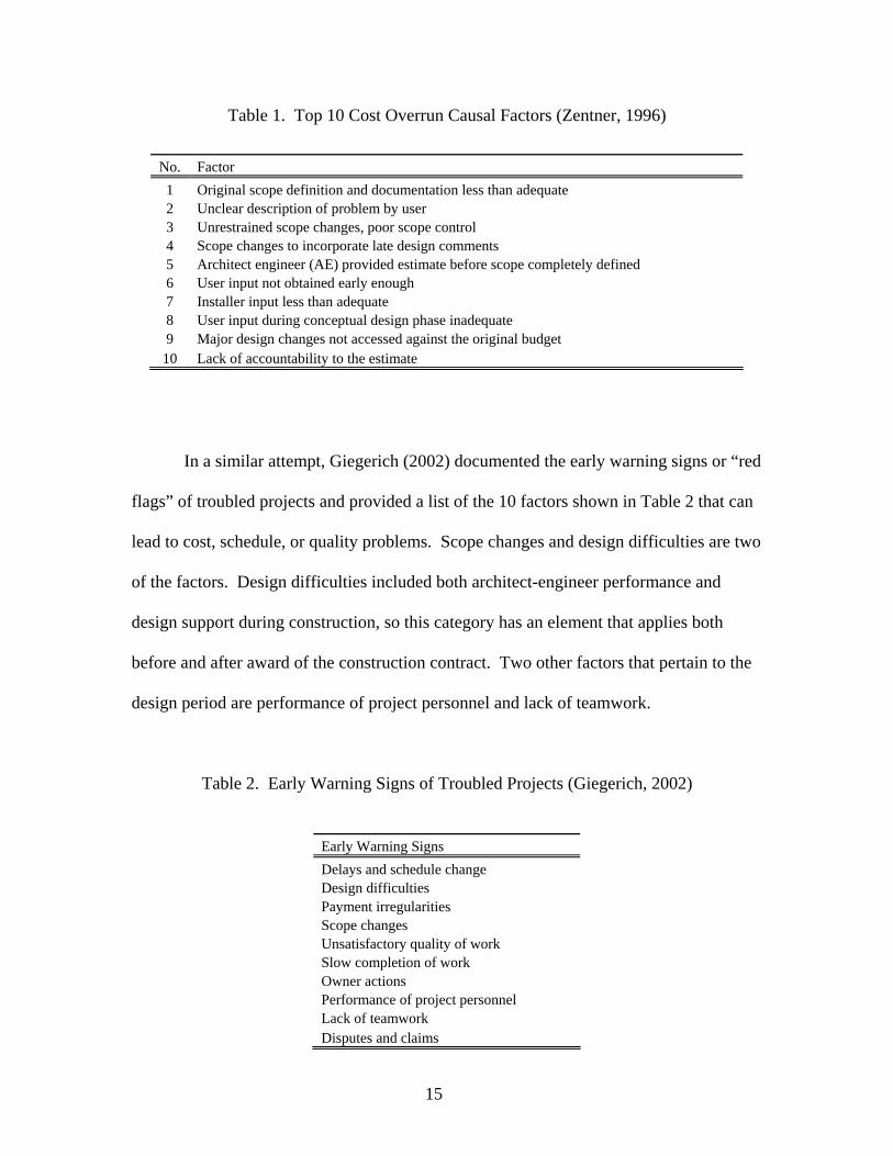
time. From this study, the researchers generated a list of the “top 10” causal factors, as

shown in Table 1. Of these factors, 80% relate directly to scope identification and

control (Zentner, 1996). The research identified poor estimating technique and poor

performance tracking as major categories as well. This study indicates a clear link

between design phase problems and an increased risk of cost overruns during the

construction phase.

15

Table 1. Top 10 Cost Overrun Causal Factors (Zentner, 1996)

No. Factor 1 Original scope definition and documentation less than adequate 2 Unclear description of problem by user 3 Unrestrained scope changes, poor scope control 4 Scope changes to incorporate late design comments 5 Architect engineer (AE) provided estimate before scope completely defined 6 User input not obtained early enough 7 Installer input less than adequate 8 User input during conceptual design phase inadequate 9 Major design changes not accessed against the original budget

10 Lack of accountability to the estimate

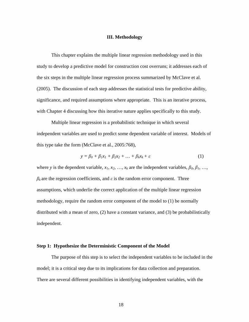
In a similar attempt, Giegerich (2002) documented the early warning signs or “red

flags” of troubled projects and provided a list of the 10 factors shown in Table 2 that can

lead to cost, schedule, or quality problems. Scope changes and design difficulties are two

of the factors. Design difficulties included both architect-engineer performance and

design support during construction, so this category has an element that applies both

before and after award of the construction contract. Two other factors that pertain to the

design period are performance of project personnel and lack of teamwork.

Table 2. Early Warning Signs of Troubled Projects (Giegerich, 2002)

Early Warning Signs Delays and schedule change Design difficulties Payment irregularities Scope changes Unsatisfactory quality of work Slow completion of work Owner actions Performance of project personnel Lack of teamwork Disputes and claims

16

In a study conducted on Federal Highway Administration projects, Harbuck

(2004) proposed that the contracting and award process itself was a potential contributor

to a project’s cost overrun. He documented three major categories of cost overruns in

highway projects: design problems, construction problems, and third party problems.

Design problems included design changes, design errors, and ambiguous specifications.

Construction problems included differing site conditions, delays, and scope additions.

Finally, third party problems included utilities, local government, and permit agencies

(Harbuck, 2004). Although the nature of the relationship was undefined, he found

evidence that cost overruns are symptomatic of contractor perceptions of risk. Low

bidders view the potential risks in an optimistic light, while high bidders perceive the

same project risk level pessimistically. With increased competition, the difference

between the low and high bid increased. The research implied a need for further

investigation into the relationship between bid climate, specifically the number of

bidders, and cost overruns. It also noted the difference between the low and median bid

seems to correlate with average cost overruns. Unfortunately, this data is not available in

the current study’s sample to allow exploration of this relationship.

Many researchers have indicated that design problems are causal factors leading

to construction cost overruns. In a study of Los Angeles public works projects, Kuprenas

and Nasr (2003) linked high design costs with poor performance during the design

period. In their study, 28 of 96 projects experienced actual design costs that greatly

exceeded the budgeted design costs. Of these projects, over two-thirds of the projects’

increased design costs could be attributed directly to “poor pre-design requiring rework

17

during the design phase” (Kuprenas and Nasr, 2003:1). This would indicate that

excessively high design costs might serve as a valid indicator of design problems.

A great deal of the research into cost overruns examines either factors beyond

project manager influence or factors unidentifiable prior to construction award. The

multiple linear regression model developed by Federle and Pigneri (1993) indicated that

funding spent on supervision correlated with increased cost overruns. Singh (2002)

identified 13 causes of claims (i.e., cost overruns); however, information relating to 10 of

these 13 causes is typically not available until either post contract award or the time of

the specific cost overrun event. Without delving into the individual causes, the overall

takeaway from the research that focuses on post contract award causes is that the overall

variance in cost overruns cannot be captured solely with information available prior to

contract award.

Conclusion

Although a predictive model based on information prior to contract award cannot

capture all of the variance in the data, the literature indicates there are relationships that

will facilitate the development of a predictive model. A number of researchers have

found meaningful relationships linking project characteristics, design phase performance,

and the contract award process with construction cost overruns. These three categories of

independent variables will serve as the framework for the initial steps of the multiple

linear regression methodology discussed in the next chapter.

18

III. Methodology

This chapter explains the multiple linear regression methodology used in this

study to develop a predictive model for construction cost overruns; it addresses each of

the six steps in the multiple linear regression process summarized by McClave et al.

(2005). The discussion of each step addresses the statistical tests for predictive ability,

significance, and required assumptions where appropriate. This is an iterative process,

with Chapter 4 discussing how this iterative nature applies specifically to this study.

Multiple linear regression is a probabilistic technique in which several

independent variables are used to predict some dependent variable of interest. Models of

this type take the form (McClave et al., 2005:768),

y = β0 + β1x1 + β2x2 + … + βkxk + ε (1)

where y is the dependent variable, x1, x2, …, xk are the independent variables, β0, β1, …,

βk are the regression coefficients, and ε is the random error component. Three

assumptions, which underlie the correct application of the multiple linear regression

methodology, require the random error component of the model to (1) be normally

distributed with a mean of zero, (2) have a constant variance, and (3) be probabilistically

independent.

Step 1: Hypothesize the Deterministic Component of the Model

The purpose of this step is to select the independent variables to be included in the

model; it is a critical step due to its implications for data collection and preparation.

There are several different possibilities in identifying independent variables, with the

19

approach depending upon the overall intent of a proposed study. In some instances, a

review of the literature indicates that certain independent variables have proved

predictive in the past. In other cases, the researcher may have a hypothesized relationship

for which he or she is attempting to provide supporting evidence. It is important to note

that selection of independent variables does not rely upon a hypothesized or demonstrated

causal relationship. For the purposes of the multiple linear regression methodology, good

independent variables correlate with the dependent variable. However, the independent

variables may only be indicators and not necessarily causal factors for the response in the

dependent variable.

Independent variables can be either quantitative, qualitative, or a combination of

both. A regression model includes qualitative variables by the creation of “dummy”

variables, which are defined to correspond to distinct levels of the qualitative variable.

The actual coding of dummy variables is arbitrary except for one key consideration. A

qualitative variable may have n distinct levels; therefore, the researcher might code n

dummy variables to correspond individually to each of these n levels. However, a

regression model can only contain a maximum of n-1 levels of the dummy variable. The

value of the intercept regression coefficient, based on the mathematics involved, includes

the nth dummy variable level.

A useful technique in identifying candidate independent variables is the use of the

analysis of variance (ANOVA) test to identify significant breakpoints in quantitative

variables. While a quantitative variable may not be predictive in itself, converting it to

qualitative dummy variables based on the breakpoints from the ANOVA test may make it

predictive. The ANOVA test is a statistical technique for comparing population means.

20

In this context, ANOVA compares the means of the dependent variable populations for

the levels of the independent variable. If the means are statistically different, the new

qualitative dummy variable qualifies for further evaluation of predictive ability. A

typical way of doing this is to visually inspect bivariate plots of quantitative independent

variables versus the dependent variable and search for possible distinct levels within the

quantitative variable. For any detected patterns, dummy variables are then coded for the

possible distinct levels of the variable of interest.

Often, a researcher may elect to “pool” candidate variables and screen them

before making the final decision of which independent variables to include in the model.

For the purposes of this study, potential independent variables were identified from past

research and a screening of all available data fields; additionally, some potential

independent variables were the result of hypothesized relationships to be tested. Only the

most predictive variables remained in the final model.

Step 2: Estimate Model Parameters

The purpose of this step is to complete the deterministic portion of the regression

model. This step uses sample data gathered on independent and dependent variables;

however, researchers normally set aside a portion of their available data for use in step 6.

After identifying the independent variables, the method of least squares is used to

determine the regression coefficients. This involves the solution of a large number of

simultaneous linear equations; therefore, researchers normally rely upon software

packages to perform the necessary calculations. The overall intent of the method of least

squares is to identify the regression coefficients that minimize the sum of the squares of

21

the difference between the predicted dependent variable values and the actual dependent

variable values. Put another way, the method of least squares finds the model that

minimizes the squared error in dependent variable predictions.

Step 3: Specify the Probability Distribution of the Random Error Term

The purpose of this step is to complete the model by specifying the

nondeterministic portion, or random error term, of the regression model. This

methodology assumes a normally distributed error term with a mean of zero. All that

remains is specification of the distribution variance or σ2. Since the actual variance is

unknown, dividing the sum of the squares for the error in the model by the difference in

the number of observations and the number of regression coefficients provides a

reasonable estimate (McClave et al., 2005).

Step 4: Check Assumptions of the Random Error Term

The outcome of the previous three steps is a fully specified multiple linear

regression model. The purpose of this step is to ensure the model meets all of the

required assumptions for proper application of the multiple linear regression

methodology. Once again, these assumptions surround the random error term of the

regression model.

First, the random error term must be normally distributed with a mean of zero.

Testing the mean of the error term only requires plotting a distribution of the residuals

and calculating the mean. For the purposes of this study, the Shapiro-Wilk test was used

to check whether the residuals were normally distributed. With the Shapiro-Wilk test, the

22

software fits a normal distribution to the residuals and then performs a goodness-of-fit

test. The null hypothesis is that the residuals are normally distributed, and the alternate

hypothesis is that the residuals are not normally distributed. The probability value (p-

value) generated in this test is compared to the designated α of 0.05 (indicating the

researcher requires a 95% confidence level in the results). If the p-value is greater than

0.05, there is not enough evidence to support the alternate hypothesis. Since the null

hypothesis cannot be rejected, the residuals are assumed to be normally distributed. If the

value is less than 0.05, there is enough evidence to indicate that the residuals are not

normally distributed.

At this point in the process, it is easy to test for statistical outliers and influential

data points. The presence of outliers in the residuals can be evidence of problems with

individual data points or the regression model itself. For a normal distribution, 95% of

all values should fall within 2 standard deviations of the mean and 99% within 3 standard

deviations. Converting the residuals to a “studentized” distribution and then plotting

them enables easy inspection for outliers. Converting residuals to studentized values

converts them to equivalent values in a normal distribution with a mean of zero and a

standard deviation of one. After this conversion, the residuals become numbers that

represent the number of standard deviations they are from zero. Therefore, any values

greater than three or less than negative three are potential outliers and require further

investigation.

Influential data points are different than statistical outliers. An influential data

point is an observation included in the model that has a disproportionate effect on

calculating the regression coefficients. The resulting effect of the data point is to “pull”

23

the regression coefficient estimates in order to account for this single data point. An

influential data points can result in a regression model that is not representative of the

overall data population because of this single point. For the purposes of this study, the

Cook’s distance statistic was used to detect influential data points. The Cook’s distance

statistic “measures the shift in the vector of regression coefficients when a particular

object is omitted” (Freund et al., 2003:86). While there are no specific rules regarding

the results of the Cook’s distance statistic, a large value warrants further investigation

into an individual observation. For this research, any value greater than 0.25 was

considered a sign that further investigation was needed.

The next assumption to be checked is whether the error term exhibits constant

variance. This study used the Breusch-Pagan test, in which the null hypothesis states that

the residuals have constant variance. The alternate hypothesis is that the residuals do not

have constant variance. The researcher records the sum of the squares of the error (SSE)

in the model and the number of observations used and then uses the same independent

variables in a regression analysis in which the dependent variable is the squared residuals

of the proposed model. This regression analysis generates a sum of squares for

regression (SSR). These three values allow calculation of a test statistic in the chi-

squared distribution with a corresponding p-value. Similar to the test for normality, this

p-value is compared to the designated α of 0.05. If the p-value is greater than 0.05, there

is not enough evidence to support the alternate hypothesis. Since the null hypothesis

cannot be rejected, the residuals are assumed to exhibit constant variance. If the p-value

is less than 0.05, there is enough evidence to indicate that the residuals do not have

constant variance.

24

The final assumption of independence is the most difficult to test. While there are

statistical tests for time-dependent data, these tests do not apply to this study. Therefore,

logical arguments must be used and a judgment made as to whether this assumption is

valid for the regression model developed in this research. The lack of ability to test this

assumption is a limitation that is discussed further in Chapter 5.

Step 5: Statistically Evaluate the Usefulness of the Model

The result of the first four steps is a fully specified regression model that has been

tested for compliance with the required assumptions. The purpose of this step is to

determine the statistical significance of the regression model. An F-test initially

determines if at least some portion of the overall model is statistically significant.

Hypothesis tests of each regression coefficient are then used to determine if the

regression model is statistically different due to the inclusion of the respective

independent variable in the regression model.

An F-test evaluates the statistical significance of the entire model; its null

hypothesis is that all regression coefficients in the model are actually zero. In other

words, the null hypothesis is that none of the regression coefficients is statistically

significant; the alternate hypothesis is that at least one of the regression coefficients is

statistically different from zero. Using an F-distribution, a p-value is generated and

compared to the designated α of 0.05. If the p-value is greater than 0.05, there is not

enough evidence to indicate the model has any statistical significance. If the p-value is

less than 0.05, there is enough evidence to reject the null hypothesis and conclude that at

least one of the regression coefficients is statistically different from zero.

25

After verifying the model has at least one significant regression coefficient,

similar hypothesis tests are performed on each regression coefficient in the model,

including the intercept term. For each regression coefficient, the null hypothesis is that

the coefficient is zero; the alternate hypothesis is that the regression coefficient is

statistically different from zero. A p-value is generated and compared to the designated α

of 0.05. If the p-value is greater than 0.05, there is not enough evidence to reject the null

hypothesis. If the p-value is less than 0.05, there is enough evidence to conclude that the

regression coefficient is statistically different from zero.

A problem of concern in a regression model, depending on its application, is

collinearity. Collinearity means that independent variables correlate more with each

other than with the dependent variable. Collinearity is a concern because it makes the

value of regression coefficients unstable. This problem can be detected using variance

inflation factors (VIFs). There are no formal criteria for using the VIF scores, but the

researcher compared the VIFs to a baseline statistic calculated by taking the inverse of

the model R2 value, explained in the next paragraph, subtracted from one (Freund et al.,

2003:110). If the VIF is greater than the baseline statistic, it is an indication that

collinearity exists with other independent variables with similarly high VIF scores. This

method is useful for models with lower R2 values and is more conservative than other

methods.

The final test of the statistical significance of the regression model is the adjusted

R2 value. The multiple linear regression methodology utilizes the method of least

squares, which chooses a model equation that minimizes the sum of the squares of the

error term (SSE). The methodology calculates the best regression equation to explain the

26

variance in the dependent variable data. The sum of squares of the regression (SSR)

refers to this explained variance. An R2 value is determined by calculating the ratio of

the variance explained, or SSR, to the total variance in the data. Ranging from 0 to 1, the

R2 value indicates the percentage of sample variance explained by the regression model.

Therefore, a higher R2 value indicates a better regression model than one with a lower

value. One weakness of this measure is that the addition of any independent variable will

improve the R2 value regardless of its statistical significance. Another weakness of the

R2 value is that it does not account for sample size. Therefore, the adjusted R2 is a better

measure of a model’s statistical significance. This value is simply the R2 of the model

adjusted to account for the total number of variables, or regression coefficients, included

in the model and the sample size. The adjusted R2 value is calculated by the equation

(McClave et al., 2005:789),

Ra2 = 1 – [(n-1)/(n-(k+1))](1-R2) (2)

where R2 is the multiple coefficient of determination, n is the number of observations in

the sample, and k is the number of regression coefficients.

Step 6: Use the Model for Prediction

The ultimate test of any model is whether it is useful in practical application. The

outcome of the previous five steps is a fully specified model tested for required

assumptions and statistically evaluated for usefulness. The purpose of this step is to

determine how well the model does in actual practice. This is typically done by using the

model to predict the dependent variable of interest for data that was not a part of the

sample used to create the model. For this study, the researcher randomly selected a

27

portion of the available data for this purpose. This data was set aside and unexamined

until completion of all previous steps through several iterations. A pre-identified

comparison metric evaluates these predictions against actual values to determine some

type of performance statistic. Normally this step attempts to demonstrate that the new

model is better than an existing practice or another model.

Conclusion

The methodology presented in this chapter serves as guidance for data analysis.

Its proper application ensures that the outcome of this process is a statistically accurate,

significant, and tested model that meets all required assumptions. Use of this

methodology allows the investigation and definition of relationships between any number

of independent variables and the dependent variable of interest. This methodology is the

most appropriate of those available for the area of interest, construction cost overruns,

and the intentions of this study.

28

IV. Results

This chapter summarizes the development of a predictive model for construction

cost overruns using available data on Air Force projects. The data collection section

discusses the source of project data and the steps used in determining a sample population

of projects with required project information. The remaining sections cover the

methodology steps described in Chapter 3.

Data Collection

Data used to develop the proposed multiple linear regression model was captured

from the Air Force’s Automated Civil Engineer System – Project Manager (ACES-PM)

module, which is an existing database used to capture project management information.

This system contains hundreds of data fields, but the use of these fields varies depending

on project type, funding source, and user needs. Therefore, the data was thoroughly

reviewed for completeness.

The data set contained 348,427 individual project entries as of August 2005. Of

these projects, approximately 24,000 were considered complete; in other words, they

contained the basic information required to calculate a construction cost overrun

percentage. After examining these records, it quickly became apparent that consistency

in the use of available data fields existed only for Air Force Military Construction

(MILCON) projects. MILCON projects are typically larger in scope and cost than other

Air Force projects; therefore, the requirements for data maintenance and upkeep appear

stricter. Further screening of the MILCON resulted in 243 projects that contained

29

information on the independent variables of interest; these projects ranged in cost from

$346,997 to $46,131,823. Of these 243 projects, 25 were randomly selected

(approximately 10%) and set aside for step 6 of the multiple linear regression

methodology; this left 218 projects to be included in the development process.

Identification of Candidate Independent Variables

The literature review in Chapter 2 identified three broad categories of independent

variables: project characteristics, design performance indicators, and contract award

process indicators. Using this framework and the requirement that data be available prior

to contract award results in the pool of candidate variables shown in Table 3. Visual

inspection of data plots and the use of ANOVA tests helped identify many of these

variables. In total, this study identified 42 independent variables for further examination

of predictive ability.

30

Table 3. Candidate Independent Variables (Bold Items Included in Final Model)

Variable Description Project Characteristics Location (Air Force Base) Geographic location of the project Major Command (MAJCOM) Agency responsible for project funding and oversight Design Agent Agency responsible for implementing a project design Construction Agent Agency responsible for oversight during construction Construction Agent (Non Air Force) The construction agent was non Air Force Construction Duration Duration specified in the construction contract in days Construction Duration < 1 year The construction contract specifies a duration less than a year Construction Duration > 2 years The construction contract specifies a duration greater than 2 years Type of Work (EEIC) Project type as specified by AF funding code Infrastructure Project The project's primary purpose involves major utility systems Housing Project The project's primary purpose involves housing units Medical Project The project's primary purpose involves medical facilities Dorm Project The project's primary purpose involves dormitories Paving Project The project's primary purpose involves asphalt or concrete paving New Construction The primary purpose is the construction of a new facility Fiscal Year (FY) The year in which the project was funded FY 2000 and Later The project was started after October 1, 1999 Design Performance Indicators Programmed Amount (PA) Construction funding budgeted at the conceptual design phase Estimate Amount (Estimate) The estimated cost at the end of the design phase Design Cost The total cost of designing the project Design Length The total time to complete the project design in days Normalized Design Length Design length divided by design cost (days/$) Normalized Design Length (Estimate) Design length divided by the estimate amount (days/$) Normalized Design Length (Cost at Award) Design length divided by the cost at award (days/$) Design Less than 3 Months The design was completed in less than 3 months Design Greater than 2 Years The design was completed in more than 2 years Design Cost % of Estimate Design cost divided by the estimate amount Design/Estimate Cost > 10% The previous variable is greater than 0.10 Design Cost % of Cost at Award Design cost divided by the cost at award Design/Cost at Award > 10% The previous variable is greater than 0.10 Estimate % of Cost at Award Estimate amount divided by the cost at award Low Estimate The estimate is less than the cost at award Estimate % of PA Estimate amount divided by the PA Estimate > PA The estimate is greater than the PA Contract Award in August The contract award occurred in August Contract Award in September The contract award occurred in September Contract Award in October The contract award occurred in October Contract Award Process Indicators Bid Protest A bid protest occurred Number of Bidders The number of bids submitted on a project High Competition > 4 Bidders The number of bids submitted on a project is more than 4 High Competition > 5 Bidders The number of bids submitted on a project is more than 5 High Competition > 9 Bidders The number of bids submitted on a project is more than 9

31

Iterative Process of Modeling

As mentioned in Chapter 3, the multiple linear regression methodology is an

iterative process. The current study was not an exception to this rule, and the model

presented in the remainder of this chapter is the result of multiple iterations. Following is

a discussion of the reasons that resulted in multiple iterations of the entire modeling

process.

Initially, no combination of independent variables could produce a model that

would pass the required tests of assumption. Specifically, the test for normality of

residuals failed even after careful selection of independent variables and the removal of

outliers and influential data points. After several dozen iterations, some other approach

became necessary. The solution to this problem was changing the dependent variable by

transforming it to the natural logarithm of the cost overrun percentage; as it turns out,

logarithmic transformations are a common solution to passing the tests of assumptions for

economic data (McClave et al., 2005).

However, this transformation has several implications for the applicability and

usefulness of the study. For example, the most fundamental impact is that it prevents the

prediction of cost underruns, which caused the exclusion of five additional projects.

After further examination of the data, eight outliers and two influential data were

removed. Histograms of studentized residuals and Cook’s distance allowed detection of

these points as described in Chapter 3. Excessively high or low cost overrun values are

the likely cause of five of the outliers; however, no cause could be identified for the

remaining outliers or the influential data points. Removing the outliers and influential

32

data points enables the model to pass the required tests of assumptions. Thus, 203

projects were used in the development of the proposed model.

Proposed Model

This study used the JMP® Statistical Discovery Software package (Copyright ©

2003 SAS Institute Inc.) to develop the multiple linear regression model presented in this

section. The software’s stepwise regression function assisted in selecting the most

statistically significant independent variables. With this function, the user specifies

statistical significance tolerances that guide the computer’s selection of independent

variables. While this is a valuable tool, a manual investigation was performed to confirm

the software tool’s selections. The final model in equation form is,

Ln (% Overrun) = -2.151-19.285x1 + 1.018 x2 + 0.140 x3 + 0.133 x4 – 0.216 x5

– 0.234 x6 – 1.008 x7 – 0.696 x8 – 0.958 x9 + 0.295 x10 (3)

where

x1 = normalized design length (design length divided by the design cost),

x2 = estimate % of cost at award (estimate amount divided by the cost at award),

x3 = design cost/cost at award > 10% (dummy variable – 1 if > 10% and 0 if ≤ 10%),

x4 = September award (dummy variable – 1 if contract award in September and 0 if not),

x5 = high competition > 9 bidders (dummy variable – 1 if >9 and 0 if ≤ 9),

x6 = FY 2000 and later (dummy variable – 1if funded after October 1, 1999 and 0 if not),

x7 = estimate % of PA (estimate amount divided by the programmed amount),

x8 = type of work is emergency MILCON – EEIC341 (dummy variable – 1 if EEIC is 341 and 0 if not),

33

x9 = type of work is housing - EEIC713 (dummy variable – 1 if EEIC is 713 and 0 if not), and

x10 = design greater than 2 years (dummy variable – 1 if > 2 years and 0 if ≤ 2 years).

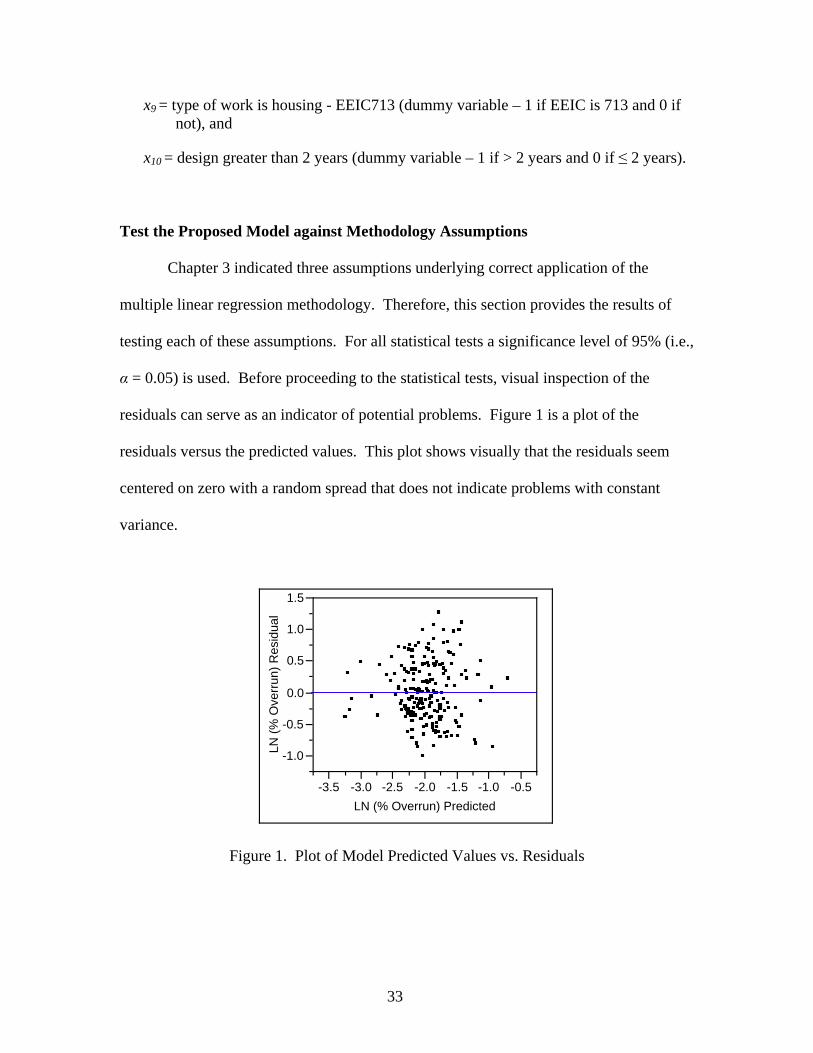
Test the Proposed Model against Methodology Assumptions

Chapter 3 indicated three assumptions underlying correct application of the

multiple linear regression methodology. Therefore, this section provides the results of

testing each of these assumptions. For all statistical tests a significance level of 95% (i.e.,

α = 0.05) is used. Before proceeding to the statistical tests, visual inspection of the

residuals can serve as an indicator of potential problems. Figure 1 is a plot of the

residuals versus the predicted values. This plot shows visually that the residuals seem

centered on zero with a random spread that does not indicate problems with constant

variance.

-1.0

-0.5

0.0

0.5

1.0

1.5

LN (%

Ove

rrun

) Res

idua

l

-3.5 -3.0 -2.5 -2.0 -1.5 -1.0 -0.5LN (% Overrun) Predicted

Figure 1. Plot of Model Predicted Values vs. Residuals

34

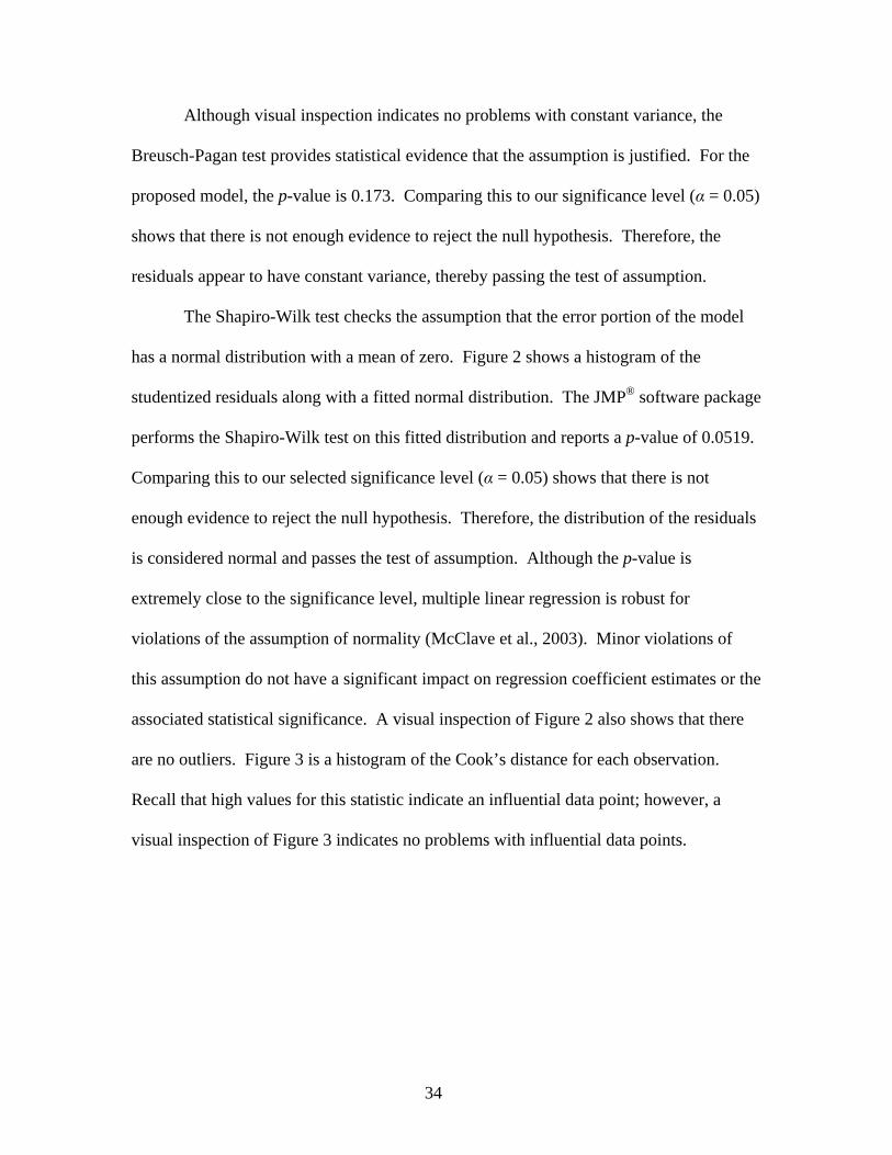
Although visual inspection indicates no problems with constant variance, the

Breusch-Pagan test provides statistical evidence that the assumption is justified. For the

proposed model, the p-value is 0.173. Comparing this to our significance level (α = 0.05)

shows that there is not enough evidence to reject the null hypothesis. Therefore, the

residuals appear to have constant variance, thereby passing the test of assumption.

The Shapiro-Wilk test checks the assumption that the error portion of the model

has a normal distribution with a mean of zero. Figure 2 shows a histogram of the

studentized residuals along with a fitted normal distribution. The JMP® software package

performs the Shapiro-Wilk test on this fitted distribution and reports a p-value of 0.0519.

Comparing this to our selected significance level (α = 0.05) shows that there is not

enough evidence to reject the null hypothesis. Therefore, the distribution of the residuals

is considered normal and passes the test of assumption. Although the p-value is

extremely close to the significance level, multiple linear regression is robust for

violations of the assumption of normality (McClave et al., 2003). Minor violations of

this assumption do not have a significant impact on regression coefficient estimates or the

associated statistical significance. A visual inspection of Figure 2 also shows that there

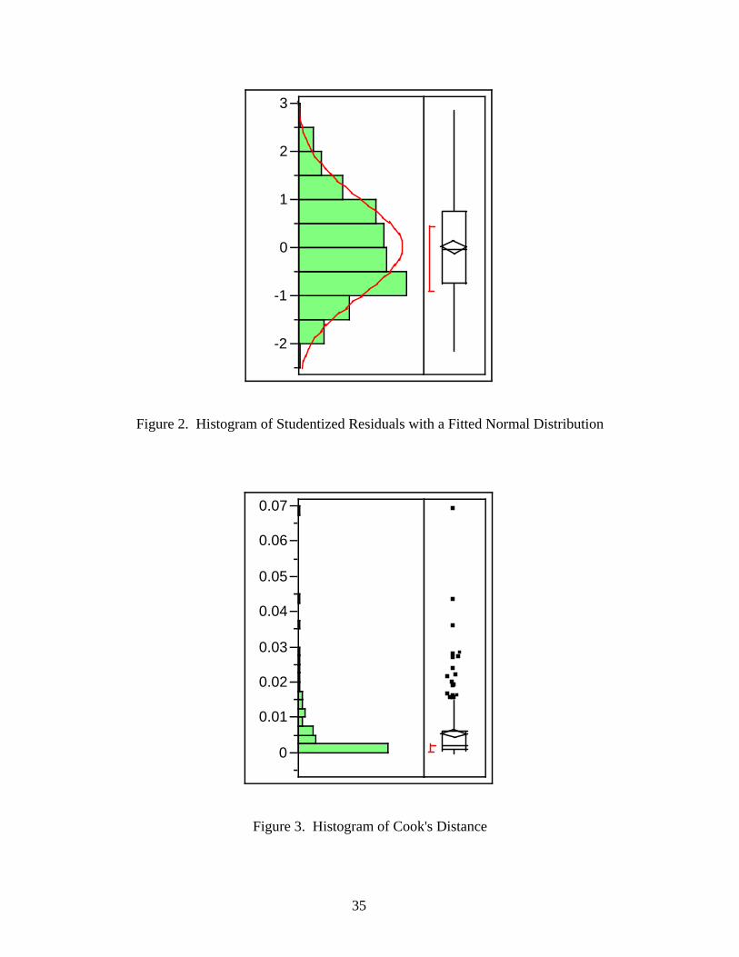
are no outliers. Figure 3 is a histogram of the Cook’s distance for each observation.

Recall that high values for this statistic indicate an influential data point; however, a

visual inspection of Figure 3 indicates no problems with influential data points.

35

-2

-1

0

1

2

3

Figure 2. Histogram of Studentized Residuals with a Fitted Normal Distribution

0

0.01

0.02

0.03

0.04

0.05

0.06

0.07

Figure 3. Histogram of Cook's Distance

36

The final assumption is independence of the observations. Unfortunately, no

statistical tests are available that apply directly to cost overrun data and this model.

Several issues might cause dependence in cost overrun errors. For example, a contractor

working several construction projects simultaneously or consecutively at a single

geographic location might cause some dependence between observations. Additionally,

large numbers of projects occurring simultaneously at a single geographic location might

also introduce dependencies. However, inspection of the project data used in the

development of this model does not indicate any situations of concern. The projects

cover a large timeframe at widely different geographic locations. Therefore, while

statistical testing of the assumption of independence is not possible, there is no evidence

to suggest violation of this assumption.

Statistically Evaluate the Usefulness of the Model

The statistical evaluation of the model’s usefulness begins with the overall F-test.

This test evaluates whether at least one of the regression coefficients is statistically

significant. Assuming the model passes this test, additional hypothesis testing determines

the statistical significance of each regression coefficient. The overall adjusted R2 value

helps interpret the amount of variance the model explains in the subject data. Finally

variance inflation scores (VIFs) are examined to assure there are no problems with

collinearity in the independent variables. The JMP® software package provides all the

previous information as part of its standard model output, and the appendix to this paper

includes this model output. The proposed model passes the F-test with a p-value less

than 0.0001; it also has an adjusted R2 value of 0.371 (unadjusted R2 = 0.402). Table 4

37

summarizes the p-values for the hypothesis tests for significance of each regression

coefficient and its associated VIF score.

Table 4. Regression Coefficient P-values and VIF Scores

Independent Variable Regression Coefficient Std Error P-value VIF

Intercept -2.151 0.266 <.0001 .

Normalized Design Length -19.285 8.588 0.026 1.145

Estimate Percent of Cost at Award 1.018 0.180 <.0001 1.110

Design/Cost at Award > 10% 0.140 0.074 0.059 1.202

Contract Award in September 0.133 0.075 0.078 1.077

High Competition >9 -0.216 0.087 0.014 1.101

FY 2000 and Later -0.234 0.078 0.003 1.158

Estimate % of Programmed Amount -1.008 0.246 <.0001 1.119

Type of Work EEIC341 (Emergency MILCON) -0.696 0.245 0.005 1.049

Type of Work EEIC713 (Housing) -0.958 0.223 <.0001 1.075

Design Greater Than 2 Years 0.295 0.124 0.018 1.119

As Table 4 indicates, two of the independent variables have p-values greater than

the designated 95% confidence level. However, these regression coefficients are

significant and non-zero with at least 90% confidence. Removing these variables from

the regression model did not decrease the R2 value significantly; however, it caused the

model to fail the tests for assumptions of the methodology. For this reason, the final

model includes both variables.

Based on the R2 value of 0.402, VIF scores greater than 1.67 would be a concern

for collinearity. As Table 4 indicates though, all VIF scores are below this value.

Therefore, the estimates of the regression coefficients are stable, meaning the

independent variables correlate with the dependent variable and not each other.

38

Use the Model for Prediction

Recall that 25 projects were set aside for preliminary testing of the model. Using

the model with these projects and comparing the predictions to the current Air Force

practice of assigning an arbitrary 5% contingency allowance provides a measure of the

model’s performance. Since the model predictions represent the natural logarithm, using

the natural exponent with the predictions provides raw percentage values in decimal form

for testing. However, this type of transformation makes it difficult to evaluate the

confidence interval of each prediction; the value returned by this transformation is the

median, and not the mean, of the confidence interval around the prediction.

A more practical approach is to set some performance limits and evaluate the

model and existing practices against the defined metric. Based on practical

considerations, a reasonable metric would be predicting the cost overrun percentage

within 5% of the actual value. Using this performance metric, the current Air Force

practice of assigning 5% contingency to projects is within the 5% of the actual overrun

percentage for only 20% of the projects tested. However, the model’s predictions are

within 5% of the actual values for 44% of the test projects. Table 5 summarizes the

results of this analysis. Additionally, the average difference between the model

prediction and the actual overrun is only -0.3% for the 25 test projects, while it is -11.2%

for current arbitrary percentages. This indicates that the average project is significantly

short in contingency funding.

39

Table 5. Comparison of Model Predictions to Current AF Practice

Actual Model Current AF

Practice Test

Project Actual

% Predicted

% Within

5% Predicted

% Within

5% 1 0.0949 0.1296 Y 0.0500 Y 2 0.1762 0.0883 N 0.0500 N 3 0.0948 0.1471 N 0.0500 Y 4 0.1151 0.2067 N 0.0500 N 5 0.1173 0.1998 N 0.0500 N 6 0.2462 0.1596 N 0.0500 N 7 0.1037 0.0998 Y 0.0500 N 8 0.2062 0.3964 N 0.0500 N 9 0.0751 0.1883 N 0.0500 Y 10 0.2937 0.1559 N 0.0500 N 11 0.1119 0.0972 Y 0.0500 N 12 0.2269 0.1292 N 0.0500 N 13 0.2360 0.1756 N 0.0500 N 14 0.1054 0.1452 Y 0.0500 N 15 0.1446 0.0990 Y 0.0500 N 16 0.0884 0.2708 N 0.0500 Y 17 0.2559 0.1234 N 0.0500 N 18 0.2335 0.1893 Y 0.0500 N 19 0.0849 0.0939 Y 0.0500 Y 20 0.1150 0.1382 Y 0.0500 N 21 0.1888 0.1247 N 0.0500 N 22 0.1074 0.1303 Y 0.0500 N 23 0.1408 0.1348 Y 0.0500 N 24 0.3591 0.2269 N 0.0500 N 25 0.1383 0.1380 Y 0.0500 N

40

Conclusion

This study resulted in a multiple linear regression model that outperforms existing

contingency funding practices using only information available prior to contract award.

Preliminary testing indicates it performs well over an extremely wide range of project

types and scopes. The model predicted 44% of test cases within 5% of the actual overrun

with an average error of -0.3%. The model performance greatly exceeds the 20%

performance metric and -11.2% average error for current practices. Chapter 5 further

discusses implications of this study.

41

V. Conclusions

This chapter discusses the key results and implications of this study, details some

of the limitations associated with the multiple linear regression model that was

developed, and provides recommendations for use of the model. Additionally, this

section presents some ideas for further research that may advance understanding of

construction cost overruns and increase the effectiveness of preventing and planning for

them.

Discussion of Results

The final regression model includes 10 independent variables shown to have a

relationship with potential cost overruns. To gain insight into these relationships, the

following paragraphs discuss each of the variables. Prior to this though, it is important to

reiterate that the model provides the natural logarithm of the predicted cost overrun

percentage in decimal form. Therefore, the discussions will reference percentages that

represent median, and not mean, values.

The most obvious observation of the modeling effort is the intercept coefficient.

This value corresponds to a base-line overrun amount of 11.63%, which greatly exceeds

the current practice of assigning 5% contingency to a construction project. This is an

indication that current practices drastically under-budget for actual overruns experienced.

From a macro perspective then, this raises questions regarding the effectiveness of

current project cost control activities and measures.

42

Normalized design length is the total length of the design period in days divided

by the total design cost. It is a measure of how much time the designer spends working

on the project normalized by the project scope. Although this variable has a relatively

small impact on the final overrun percentage, it is very easy to control and has a negative

coefficient for the entire range. Over the range of test cases in Table 5, the lowest value

decreased the overrun by 0.03% and the highest decreased it by 1.03%. This relationship

indicates that allowing designers additional time will decrease resulting overruns. This

makes logical sense and provides some assurance that design efforts have positive results

on final cost.

Estimate percent of cost at award is an indication of how well the designers

estimated the cost of the project. The sign of this coefficient is positive, indicating that it

increases the overrun. The test case data indicates that it is better to underestimate than

overestimate the cost of the project. However, this is misleading because of probable

interaction with the variable estimate percent of programmed amount. Therefore, further

investigation of this relationship is required.

If design cost is greater than 10% of the cost at the time of award, the model

indicates that cost overruns will increase. This supports the findings of Kuprenas and

Nasr (2003) in which they found that high design costs often result from design

problems. For the current research effort, the model indicates that high design costs also

indicate an increased risk of cost overruns from these design problems. In fact, ignoring

the contributions of other variables, indications of high design costs increase the baseline

cost overrun amount from 11.63% to 13.37%.

43

The contract award in September variable is unique to the fiscal year requirements

of the government, but is easily applicable to all construction projects. For the purposes

of this study, this variable indicates whether the contract award occurred in the month

immediately preceding fiscal year rollover (i.e., September). This would indicate

potential “rushing” of a project to meet funding deadlines. In these situations, awarding a

contract during this month, due primarily to funding constraints, increases the baseline

cost overrun amount from 11.63% to 13.29%.

The next variable indicates the presence of high competition, which is the only

bidder-based variable that proved significant. Based on the ANOVA analysis, the

statistically significant break point for large construction projects seems to be 10 or more

bidders. The presence of high competition, based upon the proposed model, is likely to

decrease the baseline cost overrun amount from 11.63% to 9.38%. This is similar to the

results found by Harbuck (2004).

ANOVA testing of the cost overrun percentages in the sample projects indicates

that overruns have decreased slightly in recent years. Therefore, the model includes a

variable that accounts for this trend for projects constructed after October 1, 1999.

Recent projects have a median cost overrun percentage that is 9.21% as predicted by the

model. Inclusion of this variable is necessary in the current study because of a lack of

data on recent year projects. However, this value should move into the intercept term for

practical application of the model to current projects.

Estimate percentage of programmed amount is the ratio of the final estimate to the

estimate at the concept stage of the project. This variable has a negative influence on

cost overruns according to the model; however, it most likely interacts with the estimate

44

percentage of cost at award variable. From the model, it appears that overestimation at

the concept stage is an indication of poor project definition and may result in an increased

cost overrun.

There are two separate types of work variables in the final model, emergency

Military Construction (MILCON) and housing. Emergency MILCON is work funded

because of legal requirements or other mitigating factors that make immediate

completion of the work critical. In the sample observations, these projects typically

represent simple requirements and straightforward designs. This corresponds to the

reduced median overruns predicted by the model of 5.80%. Housing work has an even

lower median overrun, ignoring other variables, of 4.46%. This relationship may

represent the fact that housing work is very “cookie-cutter” and contractors bidding on

these projects have enormous experience in bidding on and controlling these types of

projects.

The final variable in the model represents a design period that lasts longer than

two years. It indicates that a shorter design period is better, which is contrary to the

normalized design length variable. The baseline cost overrun predicted by the model

increases from 11.63% to 15.63% for excessively long designs. This is most likely an

indication of designs “placed on the shelf” and then given a quick update when funding

for the project becomes available.

The intention of this study is the prediction of cost overruns using only data that is

available prior to contract award. By framing the study in this manner, the proposed

model does not account for all the variance in cost overrun data. The adjusted R2 value

of 0.371 clearly demonstrates this fact. However, using the model to predict a best-case

45

design scenario and bid environment (where the programmed amount, estimate, and cost

at award are identical) results in a predicted overrun of approximately 7.5%. This

provides evidence of several key assumptions of this study. First, there are sources of

overrun variance not accounted for in the model. Second, even the best possible design

efforts will not eliminate cost overruns in all cases because some sources of variance are

outside the project manager’s control. Finally, even under the best circumstances, this

model predicts that the median cost overrun will exceed the 5% contingency funds

normally assigned to a construction project.

Limitations

Several limitations apply to this research. First, predicting the natural logarithm

of the cost overrun percentage means the model cannot predict a cost underrun.

However, as mentioned in the Chapter 4 section on model iteration, this only eliminated 5

of 243 projects in the sample population. Since the intention of the study is to assist in

estimating contingency fund needs, this limitation does not impair the usefulness of the

model for its intended purpose. Additionally, taking the exponent of the model

predictions returns the median or 50th percentile. This makes interpretation of confidence

intervals around the predicted value problematic and less useful for the construction

practitioner. However, the median provides a valid planning tool for construction project

contingency funds.

As with any predictive methodology, the usefulness of the model is directly

dependent upon the accuracy and range of the sample data used in its creation. This

study relies on the accuracy of the data pulled from the Air Force’s Automated Civil

46

Engineer System – Project Manger module (ACES-PM) as input by individual project

managers throughout the United States and overseas locations. While efforts were made

to minimize possible inaccuracies, there is still a possibility that inaccurate data affected

the calculation of regression coefficients. Predictive models are only truly useful within

the range of the data used to create it. In this respect, the sample population of this study

covered a comprehensive range of construction project scopes, location, costs, and other

factors; however, prediction outside the range of sample data is extrapolation beyond the

intent of the model. Additionally, the data available on the sample population limits the

independent variables examined for predictive ability. Qualitative variables such as

teamwork and communication may have a relationship with cost overruns, but capturing

this relationship is impossible within available data sources.

Finally, the scope of the study limits the total variance explained by the model.

By only using information that is available prior to contract award, sources of variance

that do not occur until post contract award are ignored and not accounted for in the

modeling efforts.

Recommendations

Usefulness of the Model

The proposed model predicted the actual cost overrun percentages within 5% for

44% of the test projects, while the current practice of assigning 5% performed to the

same level in only 20% of test cases. This indicates the model has validity and use as a

planning tool up to and including the contract award phase of a project. The average

difference between predicted and actual cost overruns was only -0.3% for the proposed

47

model, while the same statistic is -11.2% for the arbitrary assignment of a 5%

contingency. This implies that current practices will always cause a shortage in the

allocation of contingency funds, while application of the proposed model will result in a

significantly smaller shortage of contingency funds. The application of this model is a

step in the direction of correct budgeting for contingency requirements. While individual

project predictions may contain errors, the overall impact of applying the model is a

significant reduction in the net effect of under-budgeting for all projects under current

practices.

Future Research

The first area for further research is the re-accomplishment of this study using

data from projects completed after October 1, 1999 only. The fiscal year variable in the

final model represents a potential time-based trend. Further research is necessary to

determine if this reduction in overruns is a sustained trend or a result of changes in

management or design practices. An overall time trend might indicate possible market

changes that would require periodic re-evaluation. If the decrease in overruns

represented by this variable is the result of management or design practices, investigation

into the causes might shed insight into gaining further reductions.

The housing type of work variable in the final model is possible evidence of the

influence of contractor experience. Further investigation into this area may increase the

predictive ability of future model revisions and enable the inclusion of additional

variables accounting for contractor experience as it applies to other project types.

Current data gathering techniques in the Air Force did not make it possible to include this

investigation as a part of this study.

48

The interaction of the programmed amount, estimated amount, and cost at award

in the model represents a complex relationship that requires further investigation to

understand. The implications of this complex interaction are two-fold. First, these values

serve as performance metrics of the design effort. How the relationships of these three

values correspond to the quality of a design is important in understanding the impacts to

potential cost overruns. Second, understanding the relationships and their predictive

ability is critical to determining a control strategy that minimizes potential cost overruns.

As an Air Force-specific area of further research, investigation into the

effectiveness of current construction data gathering practices might improve the quality

of data captured in ACES-PM. From the data collection section of Chapter 4, less than

7% of available sample projects had the minimum requisite data fields for capturing cost

overrun information. Inconsistencies in data field use and bookkeeping practices

throughout Major Commands greatly reduces the overall effectiveness and utility of

gathered data. Further research might determine if improving the ACES-PM system

would make it more effective, either through software or policy changes.

Finally, this study indicates that no amount of design work will eliminate all

potential cost overruns. Regardless of the effort expended, it seems some cost overruns

are beyond the project manager’s control in the design phase. Research into the “point of

diminishing return” for design funding and time would be beneficial in maximizing the

return on investment for expended design effort.

49

Appendix

JMP® Regression Model Output

50

Response LN (% Overrun) Actual by Predicted Plot

-3.5

-3

-2.5

-2

-1.5

-1

-0.5LN

(% O

verr

un) A

ctua

l

-3.5 -3.0 -2.5 -2.0 -1.5 -1.0 -0.5LN (% Overrun) Predicted P<.0001RSq=0.40 RMSE=0.4743

Summary of Fit RSquare 0.402054RSquare Adj 0.370911Root Mean Square Error 0.474297Mean of Response -1.96494Observations (or Sum Wgts) 203 Analysis of Variance Source DF Sum of Squares Mean Square F RatioModel 10 29.041921 2.90419 12.9099Error 192 43.191910 0.22496 Prob > FC. Total 202 72.233831 <.0001 Parameter Estimates Term Estimate Std Error t Ratio Prob>|t| VIFIntercept -2.151282 0.26571 -8.10 <.0001 .Normalized Design Length -19.28451 8.588378 -2.25 0.0259 1.1450628Estimate Percent of Cost at Award 1.0184801 0.179565 5.67 <.0001 1.1099979Design/Cost at Award > 10% 0.1397122 0.073644 1.90 0.0593 1.2018648Contract Award in September 0.132996 0.074995 1.77 0.0777 1.0766651High Competition >9 -0.215583 0.086995 -2.48 0.0141 1.1007514FY 2000 and Later -0.233655 0.078134 -2.99 0.0032 1.157993Estimate % of Programmed Amount -1.008428 0.245572 -4.11 <.0001 1.1185188Type of Work EEIC341 (Emergency MILCON)

-0.696249 0.245281 -2.84 0.0050 1.0486791

Type of Work EEIC713 (Housing) -0.957792 0.222663 -4.30 <.0001 1.0748185Design Greater Than 2 Years 0.2953019 0.123895 2.38 0.0181 1.1193256

51

Effect Tests Source Nparm DF Sum of Squares F Ratio Prob > FNormalized Design Length 1 1 1.1342166 5.0419 0.0259Estimate Percent of Cost at Award 1 1 7.2370698 32.1708 <.0001Design/Cost at Award > 10% 1 1 0.8096502 3.5991 0.0593Contract Award in September 1 1 0.7074749 3.1449 0.0777High Competition >9 1 1 1.3814697 6.1410 0.0141FY 2000 and Later 1 1 2.0117195 8.9427 0.0032Estimate % of Programmed Amount 1 1 3.7934347 16.8629 <.0001Type of Work EEIC341 (Emergency MILCON)

1 1 1.8126056 8.0575 0.0050

Type of Work EEIC713 (Housing) 1 1 4.1624278 18.5031 <.0001Design Greater Than 2 Years 1 1 1.2779806 5.6810 0.0181 Scaled Estimates Continuous factors centered by mean, scaled by range/2 Term Scaled

EstimatePlot Estimate Std Error t Ratio Prob>|t|

Intercept -1.964937 0.033289 -59.03 <.0001Normalized Design Length -0.484138 0.215612 -2.25 0.0259Estimate Percent of Cost at Award

0.8046389 0.141863 5.67 <.0001

Design/Cost at Award > 10% 0.0698561 0.036822 1.90 0.0593Contract Award in September 0.066498 0.037498 1.77 0.0777High Competition >9 -0.107791 0.043497 -2.48 0.0141FY 2000 and Later -0.116828 0.039067 -2.99 0.0032Estimate % of Programmed Amount

-0.583984 0.142212 -4.11 <.0001

Type of Work EEIC341 (Emergency MILCON)

-0.348124 0.12264 -2.84 0.0050

Type of Work EEIC713 (Housing)

-0.478896 0.111332 -4.30 <.0001

Design Greater Than 2 Years 0.147651 0.061948 2.38 0.0181

52

Distributions Cook's D Influence LN (% Overrun)

0

0.01

0.02

0.03

0.04

0.05

0.06

0.07

Quantiles 100.0% maximum 0.06923 99.5% 0.06871 97.5% 0.02764 90.0% 0.01418 75.0% quartile 0.00607 50.0% median 0.00180 25.0% quartile 0.00051 10.0% 0.00006 2.5% 1.32e-6 0.5% 2.15e-8 0.0% minimum 2.03e-8 Moments Mean 0.0050686 Std Dev 0.0082629 Std Err Mean 0.0005799 upper 95% Mean 0.0062121 lower 95% Mean 0.0039251 N 203

53

Studentized Resid LN (% Overrun)

-2

-1

0

1

2

3

Normal(0.00094,1.00061) Quantiles 100.0% maximum 2.794 99.5% 2.786 97.5% 2.096 90.0% 1.439 75.0% quartile 0.747 50.0% median -0.047 25.0% quartile -0.744 10.0% -1.342 2.5% -1.784 0.5% -2.148 0.0% minimum -2.152 Moments Mean 0.0009386 Std Dev 1.0006109 Std Err Mean 0.0702291 upper 95% Mean 0.1394147 lower 95% Mean -0.137538 N 203 Fitted Normal Parameter Estimates Type Parameter Estimate Lower 95% Upper 95%Location Mu 0.000939 -0.137538 0.139415Dispersion Sigma 1.000611 0.911825 1.108703 Goodness-of-Fit Test Shapiro-Wilk W Test

W Prob<W .986591 0.0519

54

References

Chen, Dong, and Francis T. Hartman. “A Neural Network Approach to Risk Assessment and Contingency Allocation,” AACE International Transactions: RISK.07.01-RISK.07.06 (2000).

Department of the Air Force. The United States Air Force Project Manager’s Guide for

Design and Construction. Washington: HQ AFCEE, June 2000. Department of the Air Force. Air Education and Training Command Project Manager’s

Guide for Design and Construction. Washington: HQ AETC, Spring 2004. Federle, Mark O., and Steven C. Pigneri. “Predictive Model of Cost Overruns,”

Transactions of AACE International: L.7.1-L.7.9 (1993). Freund, Rudolf, and others. Regression Using JMP®. North Carolina: SAS Institute Inc.

and John Wiley & Sons, Inc., 2003. Giegerich, Donald B. “Early Warning Signs of Troubled Projects,” AACE International

Transactions: CDR.02.1-CDR.02.8 (2002). Harbuck, Robert H. “Competitive Bidding for Highway Construction Projects,” AACE

International Transactions: EST.09.1-EST.09.4 (2004). Kuprenas, John A., and Elhami B. Nasr. “Controlling Design-Phase Scope Creep,”

AACE International Transactions: CSC.01.1-CSC.01.5 (2003). Mantel, Samuel J., Jr. and others. Project Management in Practice. New Jersey: John

Wiley & Sons, Inc., 2005. McClave, James T., and others. Statistics for Business and Economics (9th Edition).

New Jersey: Pearson Prentice Hall, 2005. Singh, Rohit. “Be Prepared for Construction Claims – Globally,” AACE International

Transactions: CDR.04.1-CDR.04.2 (2000). Zentner, Randal S. “Accurate Estimates Start with Clear Pictures,” Transactions of

AACE International: C&S/M&C.10.1-C&S/M&C.10.6 (1996).

1

REPORT DOCUMENTATION PAGE Form Approved OMB No. 074-0188

The public reporting burden for this collection of information is estimated to average 1 hour per response, including the time for reviewing instructions, searching existing data sources, gathering and maintaining the data needed, and completing and reviewing the collection of information. Send comments regarding this burden estimate or any other aspect of the collection of information, including suggestions for reducing this burden to Department of Defense, Washington Headquarters Services, Directorate for Information Operations and Reports (0704-0188), 1215 Jefferson Davis Highway, Suite 1204, Arlington, VA 22202-4302. Respondents should be aware that notwithstanding any other provision of law, no person shall be subject to an penalty for failing to comply with a collection of information if it does not display a currently valid OMB control number. PLEASE DO NOT RETURN YOUR FORM TO THE ABOVE ADDRESS. 1. REPORT DATE (DD-MM-YYYY)

23-03-2006 2. REPORT TYPE

Master’s Thesis

3. DATES COVERED (From – To) Jun 2005 – Mar 2006

5a. CONTRACT NUMBER

5b. GRANT NUMBER

4. TITLE AND SUBTITLE Estimating Required Contingency Funds for Construction Projects using Multiple

Linear Regression 5c. PROGRAM ELEMENT NUMBER

5d. PROJECT NUMBER 5e. TASK NUMBER

6. AUTHOR(S) Cook, Jason J., Captain, USAF

5f. WORK UNIT NUMBER

7. PERFORMING ORGANIZATION NAMES(S) AND ADDRESS(S) Air Force Institute of Technology Graduate School of Engineering and Management (AFIT/EN) 2950 Hobson Street WPAFB OH 45433-7765

8. PERFORMING ORGANIZATION REPORT NUMBER AFIT/GEM/ENV/06M-02 10. SPONSOR/MONITOR’S ACRONYM(S)

9. SPONSORING/MONITORING AGENCY NAME(S) AND ADDRESS(ES) N/A

11. SPONSOR/MONITOR’S REPORT NUMBER(S)

12. DISTRIBUTION/AVAILABILITY STATEMENT APPROVED FOR PUBLIC RELEASE; DISTRIBUTION UNLIMITED.

13. SUPPLEMENTARY NOTES

14. ABSTRACT Cost overruns are a critical problem for construction projects. The common practice for dealing with cost overruns is the assignment of an arbitrary flat percentage of the construction budget as a contingency fund. This research seeks to identify significant factors that may influence, or serve as indicators of, potential cost overruns. The study uses data on 243 construction projects over a full range of project types and scopes gathered from an existing United States Air Force construction database. The author uses multiple linear regression to analyze the data and compares the proposed model to the common practice of assigning contingency funds. The multiple linear regression model provides better predictions of actual cost overruns experienced. Based on the performance metric used, the model sufficiently captures 44% of actual cost overruns versus current practices capturing only 20% The proposed model developed in this study only uses data that would be available prior to the award of a construction contract. This allows the model to serve as a planning tool throughout the concept and design phases. The model includes project characteristics, design performance metrics, and contract award process influences. This research supports prior findings of a relationship between design funding and design performance as well as the influence of the contract award process on cost overruns. While the proposed model captures 44% of actual cost overruns, its application reduces average contingency budgeting error from -11.2% to only -0.3% over the entire test sample. 15. SUBJECT TERMS Construction, Cost Overruns, Mathematical Prediction, Regression Analysis 16. SECURITY CLASSIFICATION OF: 19a. NAME OF RESPONSIBLE PERSON

Alfred E. Thal, Jr., PhD, AFIT\ENV a. REPORT

U

b. ABSTRACT

U

c. THIS PAGE

U

17. LIMITATION OF ABSTRACT

UU

18. NUMBER OF PAGES

65 19b. TELEPHONE NUMBER (Include area code) (937) 255-3636, ext 7401; e-mail: alfred.thal@afit.edu

Standard Form 298 (Rev. 8-98) Prescribed by ANSI Std. Z39-18