estimating potential community-wide energy and greenhouse gas

Energy and Environment Research; Vol. 2, No. 1; 2012 ISSN 1927-0569 E-ISSN 1927-0577

Published by Canadian Center of Science and Education

44

Estimating Potential Community-wide Energy and Greenhouse Gas Emissions Savings from Residential Energy Retrofits

Damian Pitt1, John Randolph2, David St. Jean3 & Mark Chang2 1 Urban and Regional Planning, L. Douglas Wilder School of Government and Public Affairs, Virginia Commonwealth University, Richmond, VA, USA 2 Urban Affairs and Planning, School of Public and International Affairs, Virginia Tech, Blacksburg, VA, USA 3 Maryland Energy Administration, Annapolis, MD, USA*

Correspondence: Damian Pitt, Urban and Regional Planning, L. Douglas Wilder School of Government and Public Affairs, Virginia Commonwealth University, Richmond, VA, PO Box 842028, USA. Tel: 1-804-828-7397. E-mail: [email protected]

* Any views or opinions expressed in this article are solely those of the authors and not that of the Maryland Energy Administration.

The research was funded in part by a grant from the Town of Blacksburg, Virginia.

Received: January 29, 2012 Accepted: February 14, 2012 Online Published: May 3, 2012

doi:10.5539/eer.v2n1p44 URL: http://dx.doi.org/10.5539/eer.v2n1p44

Abstract

The residential sector accounts for over 20% of U.S. primary energy consumption and offers numerous opportunities for conservation and efficiency. Chief among these is retrofitting existing homes, which can reduce annual household energy consumption while also improving indoor air quality and thermal comfort and supporting local economic development. Many U.S. localities identify residential retrofits as a major priority in their Climate Action Plans, but lack information on the extent of energy consumption and greenhouse gas (GHG) reduction that they can achieve. We present a methodology used in Blacksburg, Virginia, to estimate potential energy and GHG savings from a residential retrofit program, which we find could reduce projected year 2050 residential energy use by as much as 36%. We conclude with a discussion of the obstacles that communities face in implementing retrofit programs and steps being taken in Blacksburg to overcome those obstacles.

Keywords: urban planning, residential, energy efficiency, greenhouse gas reduction

1. Introduction

Over 1,000 U.S. cities have initiated local climate action programs to reduce their community-wide carbon footprint and mitigate global climate change, and a growing number has reached the stage of identifying implementation measures to achieve local greenhouse gas (GHG) reductions (Boswell et al., 2011). In this process cities are evaluating the potential of various measures to reduce energy use and resulting GHG emissions from their residential, commercial, and industrial sectors, local transportation patterns, and the cities’ own municipal operations. Among these potential mitigation measures, evidence suggests that energy-efficiency retrofits to existing buildings represent the biggest, fastest, cheapest, cleanest, and most long-lasting opportunity to reduce energy use and greenhouse gas emissions in cities (Choi Granade et al., 2009).

Energy for operating buildings amounts to 40% of U.S. primary energy consumption and GHG emissions (U.S. Department of Energy, 2010a). While new green buildings can reduce future energy and emissions per square foot, we will still have a legacy of older, inefficient buildings for years to come. Improving the energy efficiency of existing residential buildings is essential to accomplishing long-term energy use and GHG emission reduction and can provide multiple additional sustainability benefits. For example, rising energy prices have reduced housing affordability, forcing low-income residents to make tough budgeting decisions between rent, energy, food, and other expenses. Residential retrofits increase the energy efficiency of a home’s “building envelope” by adding insulation to the ceilings, floors, and walls, installing more efficient windows and doors, and sealing holes and insulation by-passes to reduce infiltration of outside air into the building. They can also involve upgrading to more modern, fuel-efficient heating, ventilation, and air conditioning (HVAC) systems, and

www.ccsenet.org/eer Energy and Environment Research Vol. 2, No. 1; 2012

45

replacing inefficient lighting and appliances. Such improvements can simultaneously increase thermal comfort and improve indoor air quality while reducing energy bills, thus freeing funds for other household needs. Benefits to the economy can come not only from this increased purchasing power due to reduced energy expenditures, but also by creating “green jobs” to do the retrofit work.

However, improving the energy efficiency of our existing residential buildings is no easy task. Even though energy retrofits are generally very cost effective, they suffer from transaction costs associated with poor technical and economic information, limited access to financing the initial cost of retrofits, and weak workforce capacity to provide credible information to building owners and to perform the retrofit work (U.S. Council on Environmental Quality, 2009). Furthermore, while we can easily estimate the energy use and GHG-emission savings from retrofitting a single home, the variation in housing size and type, age, occupancy and tenure status, heating and cooling systems, and structural materials makes it difficult to estimate the potential energy and climate benefits of a large-scale community-wide retrofit program.

We focus here on this latter problem and present a case study of our approach to estimating potential community-wide energy and GHG savings from residential retrofits in the town of Blacksburg, Virginia. Our approach uses readily available secondary data and relatively simple spreadsheet models, and can easily be replicated for other cities without the need for technical expertise in building construction or advanced computer modeling. This approach helps to remedy two major methodological difficulties – the lack of useful data and staff technical capacity – that have been identified as obstacles to the evaluation of local GHG mitigation options and the adoption and implementation of community climate action plans (Bailey, 2007; Betsill, 2001; Pitt & Randolph, 2009).

We begin by discussing local approaches to residential energy efficiency in the U.S. and the climate action planning process in Blacksburg that set the context for this research, followed by a review of prior studies that have quantified potential energy and GHG savings from residential retrofits. We then present our approach to estimating the potential energy and GHG savings from retrofitting single-family housing in Blacksburg. We conclude with a discussion of the significance of these results, the progress towards implementing a residential retrofit program in the Blacksburg area, and the opportunities and obstacles facing communities that wish to implement a residential retrofit program.

1.1 Residential Retrofits in Local Climate Action Planning

Many local governments have incorporated residential retrofit goals, policies, and programs into their climate action planning efforts. In their evaluation of 20 climate action plans from U.S. cities, Bassett and Shandas (2010) found that 70% of those plans included action strategies for improving the energy efficiency of existing residential buildings. Boswell et al. (2011) found similar trends in their study of 144 climate action plans. A typical objective of these plans is to reduce overall residential energy consumption by approximately 30 percent, and most plans are relatively general in describing how their energy efficiency goals can be achieved.

The Town of Blacksburg (VA) completed a community-wide energy use and GHG emissions inventory in 2008, with revisions in 2009. The revised inventory shows that the residential sector accounts for 26% of energy use in the town and 36% of resulting GHG emissions. The town conducted a public outreach process in 2009-2010, during which establishing a residential retrofit program, initiated with funds from the federal Energy Efficiency and Community Development Block Grant (EECBG) program, emerged as a major priority for implementation in the town’s climate action plan. A draft plan prepared for the town in 2011 included an objective to reduce GHG emissions from single-family homes by 66% from the years 2010-2050. It recommended a number of strategies to be implemented by the local government and the community at large, including a residential energy efficiency retrofit program.

Some climate action planning early adopter communities have already enacted aggressive policies to implement residential retrofits. For example, Berkeley and San Francisco adopted time-of-sale energy standards for existing buildings (City of Berkeley, 2011; City of San Francisco, 2009). Seattle’s municipal utility has offered demand side retrofits for thirty years, saving one million megawatt hours (MWh) per year by 2006 (Seattle City Light, 2011). Philadelphia’s residential weatherization program upgraded nearly 1,100 low-income homes in the 2010 fiscal year (Philadelphia Housing Development Corporation, 2010). New York and Portland, among other cities, participate in multi-agency public-private partnerships to provide building energy services (City of Portland, 2011; Pratt Center for Community Development, 2011).

However, most local climate action plans are rather vague when estimating the impacts of residential retrofit programs. The city of Chicago’s Climate Action Plan includes perhaps the most detailed evaluation of retrofit potential. Their analysis concludes that residential retrofits can reduce per-building energy demand by 30%


46

through a combination of building envelope efficiency, water heating, and lighting upgrades (Center for Neighborhood Technology, 2008). Boulder, Colorado, a college town with similar demographics to Blacksburg (e.g., higher-than-average percentages of renter-occupied and multi-family units) estimates in its Climate Action Plan that weatherization efforts could reduce residential energy bills by 20-25%. Boulder also conducted a pilot study in which five homes received energy efficiency retrofits that included new high efficiency furnaces. These homes experienced savings of around 50% on their heating bills (City of Boulder, 2006).

1.2 Studies of Energy and GHG Savings from Residential Retrofits

Much of the academic research on residential energy efficiency focuses on residential behavior with respect to energy conservation and efficiency investments (e.g., Parker, Rowlands & Scott, 2005). Many of the prior studies on building performance focus on specific efficiency improvements, such as window replacement, heating system upgrades, etc., while others analyze energy efficiency potential in commercial or institutional buildings (e.g., Yalcintas & Kaya, 2009). We focus here on those that evaluate whole building energy efficiency potential in the residential sector.

In the 1980s researchers at the Lawrence Berkeley Laboratory maintained a database of the before-and-after energy performance outcomes of over 100 residential retrofit programs in the U.S. and Canada. Initial findings included an average space-heating energy use reduction of 20-30% (Goldman, 1985; Wall et al., 1983), while a follow-up study found a median average annual electricity savings of 16% (Cohen et al., 1991). Other studies from that era produced similar results, generally around 20-40% of space heating energy demand and 10-20% of total household energy demand (Hirst & Goeltz, 1985; Brown & Berry, 1993; Randolph et al., 1991). More recently, a number of European researchers have modeled the potential effects of residential energy efficiency retrofits in their respective regions. Hens et al. (2001) noted that residential energy use in Belgium could, in theory, be reduced by 75% if all homes were built or retrofitted to the International Energy Agency’s recommended Solar Low Energy House standard. In a study of new residential construction in Ireland, Dineen and Ó Gallachóir (2011) estimated that space heating demand had already fallen 28% from 2001 to 2007, and that proposed new efficiency policies could reduce that demand to 75% below the 2001 level. For individual homes, Verbeeck and Hens (2005) found that primary energy consumption in an individual rural dwelling could be reduced by about 50%. The greatest opportunities for residential energy efficiency are demonstrated by the German “passivhaus” principle, which can reduce space heating energy consumption to 80% below that of comparable conventional homes, with total household primary energy use savings of 50% (Schneiders, 2003).

Other studies have found less optimistic results for residential energy efficiency. Uihlein (2010), for example, envisioned potential energy use and GHG savings of only 14% from “cost-optimal” retrofits in the EU, but it should be noted that this scenario included only structural efficiency measures without any HVAC efficiency improvements. Similarly, Lloyd et al. (2008) found that retrofits to public housing units in southern New Zealand reduced household energy consumption by only 5-9%, pointing to the potential for retrofits to result in improved thermal comfort rather than energy savings, particularly when the participants are low-income households in areas of extreme winter weather.

The U.S. Department of Energy’s (DOE) Weatherization Assistance Program (WAP), which provides funding for retrofits to low-income homes, reports an average savings of 32% on clients’ heating bills (U.S. Department of Energy, 2010b). These savings can be even greater in colder climates, where improved insulation and reduced infiltration can reduce space heating and cooling demands by 50% (Moomaw & Johnston, 2008). The impacts and cost-effectiveness of the WAP are regularly evaluated at the state level, and DOE produced meta-evaluations of the program’s performance based on these state analyses in 1997, 1999, and 2005 (Schweitzer, 2005). The agency is currently conducting a new nation-wide evaluation of the WAP (Energy Center of Wisconsin, 2011).

The U.S. national HERS rating system created by the Residential Energy Systems Network (RESNET) was originally developed for new homes but is now used for existing homes as well. The revised rating scores a house meeting the 2004 International Energy Conservation Code at 100 and a zero energy home at 0. The HERS served as the basis for the Home Energy Score, the residential energy retrofit rating system developed by Lawrence-Berkeley National Laboratory for U.S. DOE’s home energy retrofit rating program (for more on home rating and audits systems see U.S. DOE, 2010a, 2010b).

Our case study addresses a void in the academic literature, specifically the lack of studies evaluating the potential impacts of residential energy retrofits at the community scale.

2. Estimation of Residential Energy Retrofits in Blacksburg

The following sections describe the four steps we took to evaluate those potential GHG savings in Blacksburg: estimate local residential energy demand by end-use; create baseline models for space heating energy demand in


47

typical electric and natural gas heated homes; estimate the potential space heating energy demand savings from retrofits to those typical homes; and extrapolate those per-unit savings to all single-family homes in the community.

2.1 Estimate Local End-use Residential Energy Demand

Our method for estimating local energy demand by end use, summarized in Figure 1, was based on data from the U.S. Energy Information Administration’s Residential Energy Consumption Survey (RECS) (U.S. Department of Energy, 2005). The reliability of the RECS survey data is occasionally questioned given its relatively small sample size (e.g., Brown & Logan 2008; Randolph, 2008), but it is the only source of average annual residential energy consumption data that matches the Census breakdown of housing unit types, and it has been used as a primary data source in several other published works (e.g., Ewing & Rong, 2008; Kaza, 2010). The RECS survey was updated in 2009, but results on energy consumption and expenditures had not been released by the time of this study.

Figure 1. Steps to estimating end-use residential energy consumption

The RECS data provides average annual residential energy consumption by end use (space heating, air conditioning, water heating, refrigerators, and lighting / other), broken down by tenure (renter vs. owner), units in structure (single family homes vs. townhomes, apartments, etc.), and climate, among other factors. Residences in the same “climate zone” as Blacksburg – areas that average less than 2,000 cooling-degree-days and between 4,000 and 5,499 heating degree days per year – consume about 7% more energy annually than the national average, including 17.5% more for space heating. To model local conditions in Blacksburg we used these ratios of energy consumption in our climate zone to the national average to adjust the RECS’ detailed breakdown of end use energy consumption by tenure and units in structure. We then multiplied those adjusted end-use energy consumption figures by the number of units of each housing type in 2005, as derived from U.S. Census 2000 and


48

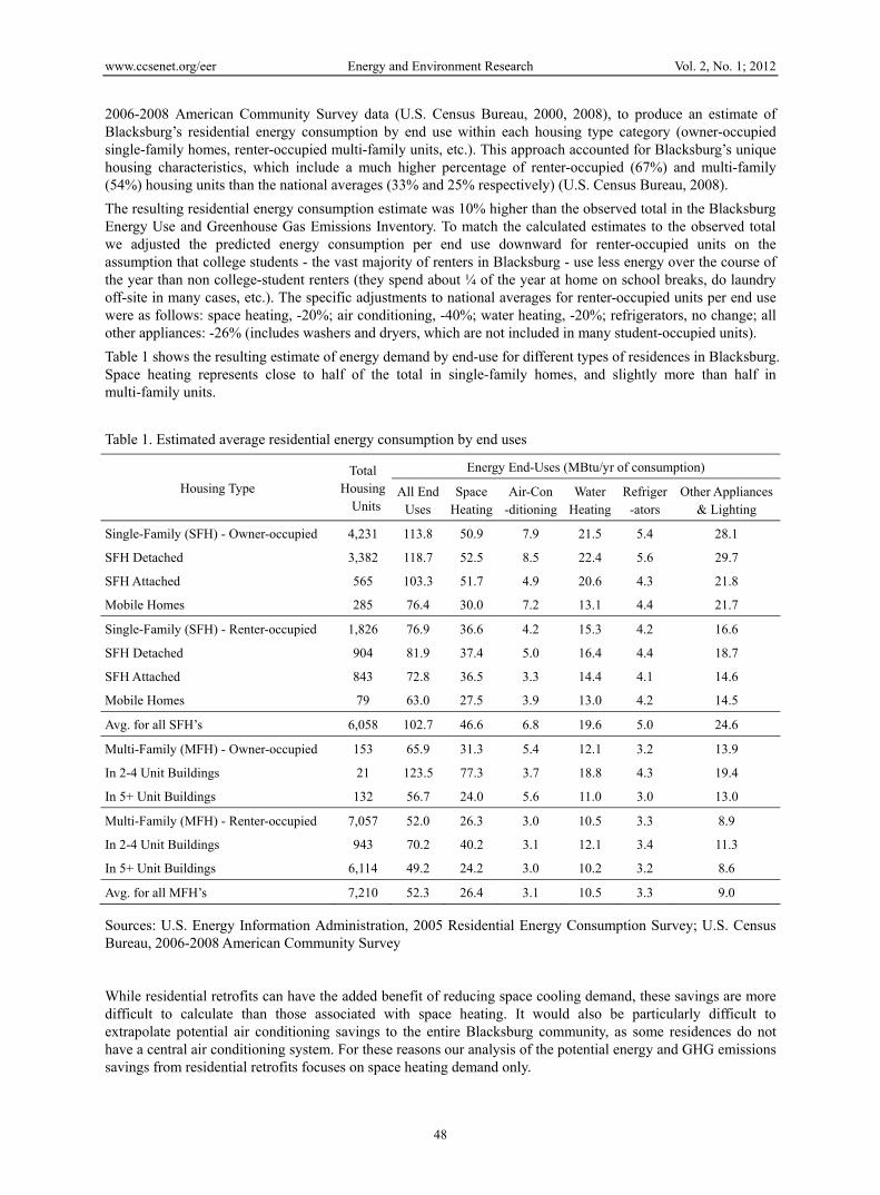
2006-2008 American Community Survey data (U.S. Census Bureau, 2000, 2008), to produce an estimate of Blacksburg’s residential energy consumption by end use within each housing type category (owner-occupied single-family homes, renter-occupied multi-family units, etc.). This approach accounted for Blacksburg’s unique housing characteristics, which include a much higher percentage of renter-occupied (67%) and multi-family (54%) housing units than the national averages (33% and 25% respectively) (U.S. Census Bureau, 2008).

The resulting residential energy consumption estimate was 10% higher than the observed total in the Blacksburg Energy Use and Greenhouse Gas Emissions Inventory. To match the calculated estimates to the observed total we adjusted the predicted energy consumption per end use downward for renter-occupied units on the assumption that college students - the vast majority of renters in Blacksburg - use less energy over the course of the year than non college-student renters (they spend about ¼ of the year at home on school breaks, do laundry off-site in many cases, etc.). The specific adjustments to national averages for renter-occupied units per end use were as follows: space heating, -20%; air conditioning, -40%; water heating, -20%; refrigerators, no change; all other appliances: -26% (includes washers and dryers, which are not included in many student-occupied units).

Table 1 shows the resulting estimate of energy demand by end-use for different types of residences in Blacksburg. Space heating represents close to half of the total in single-family homes, and slightly more than half in multi-family units.

Table 1. Estimated average residential energy consumption by end uses

Housing Type Total

Housing Units

Energy End-Uses (MBtu/yr of consumption)

All EndUses

Space Heating

Air-Con-ditioning

Water Heating

Refriger -ators

Other Appliances& Lighting

Single-Family (SFH) - Owner-occupied 4,231 113.8 50.9 7.9 21.5 5.4 28.1

SFH Detached 3,382 118.7 52.5 8.5 22.4 5.6 29.7

SFH Attached 565 103.3 51.7 4.9 20.6 4.3 21.8

Mobile Homes 285 76.4 30.0 7.2 13.1 4.4 21.7

Single-Family (SFH) - Renter-occupied 1,826 76.9 36.6 4.2 15.3 4.2 16.6

SFH Detached 904 81.9 37.4 5.0 16.4 4.4 18.7

SFH Attached 843 72.8 36.5 3.3 14.4 4.1 14.6

Mobile Homes 79 63.0 27.5 3.9 13.0 4.2 14.5

Avg. for all SFH’s 6,058 102.7 46.6 6.8 19.6 5.0 24.6

Multi-Family (MFH) - Owner-occupied 153 65.9 31.3 5.4 12.1 3.2 13.9

In 2-4 Unit Buildings 21 123.5 77.3 3.7 18.8 4.3 19.4

In 5+ Unit Buildings 132 56.7 24.0 5.6 11.0 3.0 13.0

Multi-Family (MFH) - Renter-occupied 7,057 52.0 26.3 3.0 10.5 3.3 8.9

In 2-4 Unit Buildings 943 70.2 40.2 3.1 12.1 3.4 11.3

In 5+ Unit Buildings 6,114 49.2 24.2 3.0 10.2 3.2 8.6

Avg. for all MFH’s 7,210 52.3 26.4 3.1 10.5 3.3 9.0

Sources: U.S. Energy Information Administration, 2005 Residential Energy Consumption Survey; U.S. Census Bureau, 2006-2008 American Community Survey

While residential retrofits can have the added benefit of reducing space cooling demand, these savings are more difficult to calculate than those associated with space heating. It would also be particularly difficult to extrapolate potential air conditioning savings to the entire Blacksburg community, as some residences do not have a central air conditioning system. For these reasons our analysis of the potential energy and GHG emissions savings from residential retrofits focuses on space heating demand only.


49

2.2 Prepare Baseline Models to Estimate Space Heating Demand in Single-family Homes

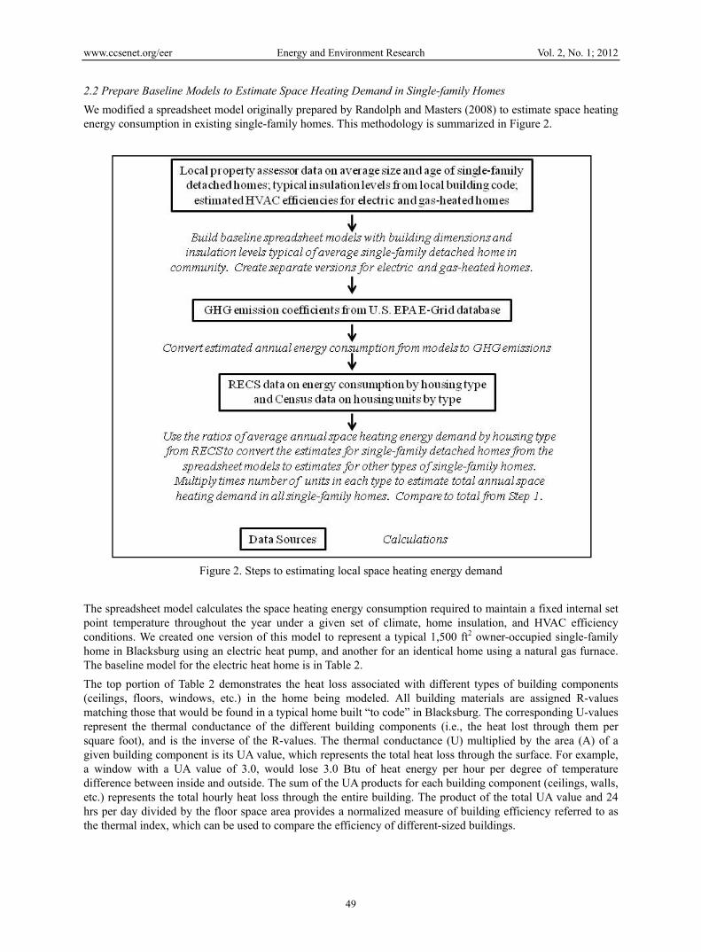
We modified a spreadsheet model originally prepared by Randolph and Masters (2008) to estimate space heating energy consumption in existing single-family homes. This methodology is summarized in Figure 2.

Figure 2. Steps to estimating local space heating energy demand

The spreadsheet model calculates the space heating energy consumption required to maintain a fixed internal set point temperature throughout the year under a given set of climate, home insulation, and HVAC efficiency conditions. We created one version of this model to represent a typical 1,500 ft2 owner-occupied single-family home in Blacksburg using an electric heat pump, and another for an identical home using a natural gas furnace. The baseline model for the electric heat home is in Table 2.

The top portion of Table 2 demonstrates the heat loss associated with different types of building components (ceilings, floors, windows, etc.) in the home being modeled. All building materials are assigned R-values matching those that would be found in a typical home built “to code” in Blacksburg. The corresponding U-values represent the thermal conductance of the different building components (i.e., the heat lost through them per square foot), and is the inverse of the R-values. The thermal conductance (U) multiplied by the area (A) of a given building component is its UA value, which represents the total heat loss through the surface. For example, a window with a UA value of 3.0, would lose 3.0 Btu of heat energy per hour per degree of temperature difference between inside and outside. The sum of the UA products for each building component (ceilings, walls, etc.) represents the total hourly heat loss through the entire building. The product of the total UA value and 24 hrs per day divided by the floor space area provides a normalized measure of building efficiency referred to as the thermal index, which can be used to compare the efficiency of different-sized buildings.


50

Table 2. Baseline model for existing single-family home – electric heat

Building Components Area (ft2) R-Value

(Thermal Resistance)U-Value

(Thermal Conductance) UA % of UA

Ceiling 1,500 30.0 0.033 50.0 10%

Windows 250 1,6 0.625 156.3 33%

Doors 60 2.5 0.400 24.0 5%

Walls 970 12.5 0.080 77.4 16%

Floors 1,500 30.0 0.033 50.0 10%

Infiltration / Ventilation Volume (ft3) Air Changes Per Hour Efficiency UA % of UA

Infiltration 12,000 0.55 NA 118.8 25%

Ventilation 12,000 0.00 70% 0.0 0%

TOTAL UA (Btu/hroF) = 476.46

Thermal Index (Btu/ft2 oF-day) = 7.6

Additional Assumptions:

Fuel Price (per million Btu) 35.60 $

Furnace Efficiency 190%

Distribution Efficiency 75%

Internal gains, qint 3,000 Btu/hr

Internal set point, Ti 68.75 oF

Heating Degree Days (HDD65) 5,052 oF d/yr

Design temperature -5 oF

Energy Consumption Results:

Balance Point Temp (Tbal) 62.5 oF

HDD @ Tbal 4,492 oF d/yr

Delivered energy (Qdel) 51.4 Million Btu/yr

Fuel Consumption (Qfuel) 36.0 Million Btu/yr

Annual Fuel Bill $1,391 per year

Annual GHG Emissions 7.5 Metric tonnes CO2-e (at 1.56 lbs/kWh)

The models also include a value for air changes per hour (ACH), which represents the heat loss associated with the permeability of building components and infiltration of outside air through gaps in the building structure. Retrofitting the building envelope reduces this leakage, but comprehensive retrofits can potentially result in an unhealthy lack of ventilation. Industry experts recommend an ACH of at least 0.35 through a combination of infiltration and mechanical ventilation.

The values for internal heat gains (Qint) account for the heat contributed to the interior environment by occupants, lighting, electrical equipment, and cooking. This factor is important when calculating the balance point temperature (Tbal), which is the temperature to which the heating system must heat the home in order to achieve the internal set point temperature. Specifically, the ratio of UAtot to Qint is subtracted from the internal set point to determine Tbal. The internal set points for both models are set at 68.75 o F, which allows the average estimated total heating energy demand from the two models to match the per-unit residential heating demand estimated for single-family detached homes in Blacksburg as shown in Table 1.

The Qdel value in the table represents the amount of heat that would need to be delivered to the home to maintain the constant set point temperature of 68.75oF for the entire home heating season. Finally, the Qfuel value is the amount of fuel consumed to provide that quantity of delivered heat, taking into account the efficiency of the HVAC system. The electric heat baseline model assumes an air-source heat pump with a rated heating season performance factor (HSPF) of 6.5, which translates to a functional efficiency of 190%. Because these systems transfer heat from the outside air to the indoor conditioned space they are able to deliver more energy in heat than they consume in electricity. The 75% distribution efficiency assumes a forced-air distribution system with


51

leaky ducts. This results in an estimated annual space heating energy consumption of 36.0 million Btu, which translates to an annual fuel bill of about $1,391 at $0.12 / kWh and produces 7.5 tonnes of CO2-equivalent GHG emissions.

The GHG conversion rate was derived from the U.S. Environmental Protection Agency’s e-Grid data for Blacksburg’s electric grid sub-region (RFC West), in which 72.9% of electricity is generated from coal, 3.75% from natural gas and other fossil fuels, 0.3% from biomass, and the remainder from non GHG-emitting nuclear (22.3%), hydro-electric (0.6%), and wind power (0.1%) (U.S. Environmental Protection Agency, 2010). The e-Grid data for RFC West shows a carbon dioxide emission rate of 1,551.52 lb/megawatt-hour (MWh), plus rates of 24.30 lb/gigawatt-hour (GWh) for methane and 31.48 lbs/GWh for nitrous oxide. The emission rates for methane and nitrous oxide were multiplied by factors of 25:1 and 298:1 respectively to convert them to CO2-equivalent emissions (U.S. Department of Energy, 2007). This adds up to 1,559.71 lbs CO2-e/MWh, which converts to 0.2078 metric tonnes CO2-e per 1 million Btu of electricity consumption.

Table 3 summarizes the baseline model for an identical owner-occupied single-family home with a natural gas furnace. All of the assumptions are the same as those shown in the electric heat model, except for the furnace efficiency and fuel price. The furnace efficiency of 80% is typical for equipment installed prior to 1992. The estimated 83.5 MBtu/year of space heating demand in this model is much higher than that of the electric-heated home because of the lower efficiency of the natural gas furnace. However, the much lower fuel price ($14.00/million Btu) and carbon coefficient (11.71 lbs CO2-e per therm, or 0.0532 tonnes/million Btu) for natural gas results in about 60% the GHG emissions and a slightly lower fuel bill compared to the electric-heated home.

Table 3. Baseline model for existing single-family home – natural gas heat

Building Components Area (ft2) R-Value

(Thermal Resistance)U-Value

(Thermal Conductance) UA % of UA

Ceiling 1,500 30.0 0.033 50.0 10%

Windows 250 1,6 0.625 156.3 33%

Doors 60 2.5 0.400 24.0 5%

Walls 970 12.5 0.080 77.4 16%

Floors 1,500 30.0 0.033 50.0 10%

Infiltration / Ventilation Volume (ft3) Air Changes Per Hour Efficiency UA % of UA

Infiltration 12,000 0.55 NA 118.8 25%

Ventilation 12,000 0.00 70% 0.0 0%

TOTAL UA (Btu/hroF) = 476.46

Thermal Index (Btu/ft2oF-day) = 7.6

Additional Assumptions:

Fuel Price (per million Btu) 14.00 $

Furnace Efficiency 80%

Distribution Efficiency 75%

Internal gains, qint 3,000 Btu/hr

Internal set point, Ti 68.75 oF

Heating Degree Days (HDD65) 5,052 oF d/yr

Design temperature -5 oF

Energy Consumption Results:

Balance Point Temp (Tbal) 62.5 oF

HDD @ Tbal 4,492 oF d/yr

Delivered energy (Qdel) 51.4 Million Btu/yr

Fuel Consumption (Qfuel) 85.6 Million Btu/yr

Annual Fuel Bill $1,306 per year

Annual GHG Emissions 4.6 Metric tonnes CO2-e (at 11.71 lbs/therm)


52

To double-check the validity of these models, we used them to estimate the average space heating energy consumption for all owner-occupied single-family detached homes in Blacksburg, and compared that value to the average derived from the RECS data in Table 1. The 2000 U.S. Census indicated that 61% of homes in Blacksburg were primarily heated with electricity, 29% with natural gas, and the remaining 10% with “other fuels” such as propane and wood. Subsequent American Community Survey reports from the Census Bureau have shown the electricity and natural gas shares increasing to 65% and 28% respectively, with the “other fuels” share decreasing to 6.7% (U.S. Census Bureau, 2010). Census 2010 data on home heating fuels was not yet available at the time of this analysis. For this study we disregarded the “other fuels” due to their diminishing role in home heating and assumed that 67% of homes in Blacksburg are electric heated and 33% use natural gas heat. Multiplying the annual fuel consumption figures for electric and gas-heated homes from Tables 2 and 3 times these respective percentages, and then by the total number of owner-occupied single-family detached homes, results in a total space heating energy consumption estimate of 177,094 MBtu/yr for those homes. This works out to a combined average of 52.4 MBtu/yr for owner-occupied single-family detached homes, nearly identical to the value in Table 1 estimated from the RECS data.

We then estimated the per-unit energy consumption for other types of single-family homes (e.g., attached owner-occupied) by multiplying the Qfuel values for the baseline electric and gas-heated homes times the respective ratios of the “combined average” values shown in Table 1. For example, the ratio of space heating demand in owner-occupied attached homes to owner-occupied detached homes in Table 1 is 0.985, and multiplying the Qfuel values from Tables 2 and 3 times this ratio results in values of 35.4 MBtu/yr for electric-heated and 85.6 for gas-heated owner-occupied attached homes. Table 4 shows the results of these calculations for all forms of single-family homes, along with the total space heating energy consumption from each home type and the re-calculated averages for each housing type.

Table 4. Estimate of single-family home heating demand from baseline models

Housing Type Total Housing

Units

Estimated Energy Consumption (MBtu/yr)

Per-Unit Electric

Per-Unit Nat Gas

Total - Electric

Total - Nat Gas

Combined Total

Combined Average

Owner-occupied 4,231 34.9 82.9 98,897 115,822 214,719 50.7

SFH Detached 3,382 36.0 85.6 81,567 95,527 177,094 52.4

SFH Attached 565 35.4 84.3 13,409 15,704 29,113 51.5

Mobile Homes 285 20.5 48.8 3,921 4,592 8,512 29.9

Renter-occupied 1,826 25.0 59.6 30,650 35,896 66,546 36.4

SFH Detached 904 25.6 61.0 15,525 18,181 33,706 37.3

SFH Attached 843 25.0 59.4 14,126 16,544 30,670 36.4

Mobile Homes 79 18.8 44.7 999 1,171 2,170 27.4

Avg. for all SFH’s 6,058 31.9 75.9 129,547 151,718 281,265 46.4

These combined average scores shown in Table 4 mirror closely those shown in Table 1 from the RECS data.

2.3 Calculate Potential Per-unit Energy Consumption and GHG Emissions Savings from Building Energy Efficiency

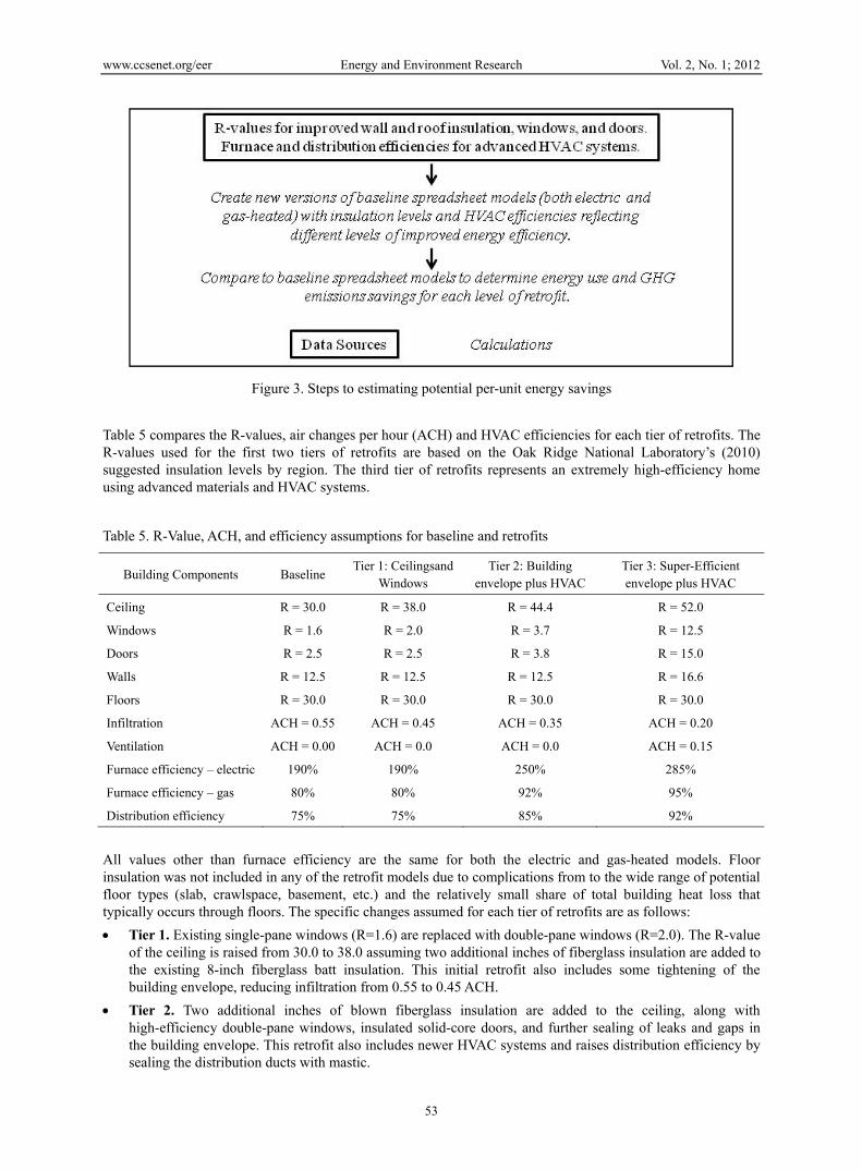
Having verified the accuracy of the baseline models, we then created additional versions of both to represent three levels of potential energy efficiency retrofits. This process is summarized in Figure 3. The three “tiers” of retrofits included upgrades to ceilings and windows (Tier 1), upgrades to the full building envelope and HVAC system (Tier 2), and super-efficient upgrades to the building envelope and HVAC system (Tier 3).


53

Figure 3. Steps to estimating potential per-unit energy savings

Table 5 compares the R-values, air changes per hour (ACH) and HVAC efficiencies for each tier of retrofits. The R-values used for the first two tiers of retrofits are based on the Oak Ridge National Laboratory’s (2010) suggested insulation levels by region. The third tier of retrofits represents an extremely high-efficiency home using advanced materials and HVAC systems.

Table 5. R-Value, ACH, and efficiency assumptions for baseline and retrofits

Building Components Baseline Tier 1: Ceilingsand

Windows Tier 2: Building

envelope plus HVACTier 3: Super-Efficient envelope plus HVAC

Ceiling R = 30.0 R = 38.0 R = 44.4 R = 52.0

Windows R = 1.6 R = 2.0 R = 3.7 R = 12.5

Doors R = 2.5 R = 2.5 R = 3.8 R = 15.0

Walls R = 12.5 R = 12.5 R = 12.5 R = 16.6

Floors R = 30.0 R = 30.0 R = 30.0 R = 30.0

Infiltration ACH = 0.55 ACH = 0.45 ACH = 0.35 ACH = 0.20

Ventilation ACH = 0.00 ACH = 0.0 ACH = 0.0 ACH = 0.15

Furnace efficiency – electric 190% 190% 250% 285%

Furnace efficiency – gas 80% 80% 92% 95%

Distribution efficiency 75% 75% 85% 92%

All values other than furnace efficiency are the same for both the electric and gas-heated models. Floor insulation was not included in any of the retrofit models due to complications from to the wide range of potential floor types (slab, crawlspace, basement, etc.) and the relatively small share of total building heat loss that typically occurs through floors. The specific changes assumed for each tier of retrofits are as follows:

Tier 1. Existing single-pane windows (R=1.6) are replaced with double-pane windows (R=2.0). The R-value of the ceiling is raised from 30.0 to 38.0 assuming two additional inches of fiberglass insulation are added to the existing 8-inch fiberglass batt insulation. This initial retrofit also includes some tightening of the building envelope, reducing infiltration from 0.55 to 0.45 ACH.

Tier 2. Two additional inches of blown fiberglass insulation are added to the ceiling, along with high-efficiency double-pane windows, insulated solid-core doors, and further sealing of leaks and gaps in the building envelope. This retrofit also includes newer HVAC systems and raises distribution efficiency by sealing the distribution ducts with mastic.


54

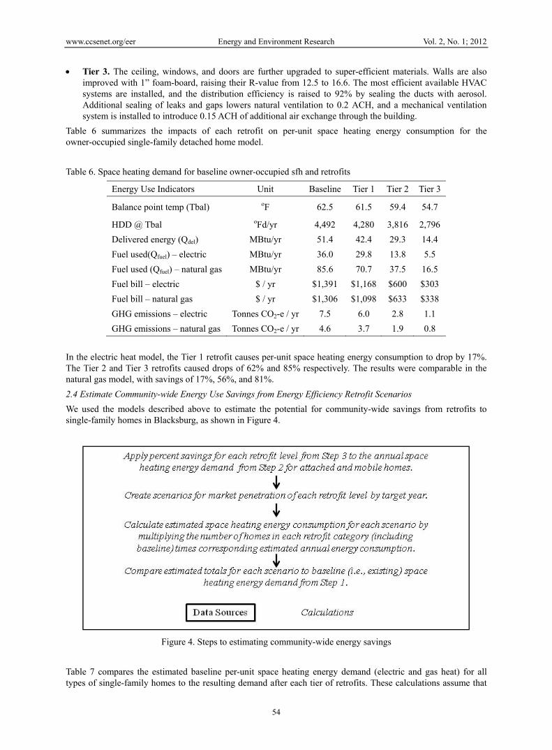
Tier 3. The ceiling, windows, and doors are further upgraded to super-efficient materials. Walls are also improved with 1” foam-board, raising their R-value from 12.5 to 16.6. The most efficient available HVAC systems are installed, and the distribution efficiency is raised to 92% by sealing the ducts with aerosol. Additional sealing of leaks and gaps lowers natural ventilation to 0.2 ACH, and a mechanical ventilation system is installed to introduce 0.15 ACH of additional air exchange through the building.

Table 6 summarizes the impacts of each retrofit on per-unit space heating energy consumption for the owner-occupied single-family detached home model.

Table 6. Space heating demand for baseline owner-occupied sfh and retrofits

Energy Use Indicators Unit Baseline Tier 1 Tier 2 Tier 3

Balance point temp (Tbal) oF 62.5 61.5 59.4 54.7

HDD @ Tbal oFd/yr 4,492 4,280 3,816 2,796

Delivered energy (Qdel) MBtu/yr 51.4 42.4 29.3 14.4

Fuel used(Qfuel) – electric MBtu/yr 36.0 29.8 13.8 5.5

Fuel used (Qfuel) – natural gas MBtu/yr 85.6 70.7 37.5 16.5

Fuel bill – electric $ / yr $1,391 $1,168 $600 $303

Fuel bill – natural gas $ / yr $1,306 $1,098 $633 $338

GHG emissions – electric Tonnes CO2-e / yr 7.5 6.0 2.8 1.1

GHG emissions – natural gas Tonnes CO2-e / yr 4.6 3.7 1.9 0.8

In the electric heat model, the Tier 1 retrofit causes per-unit space heating energy consumption to drop by 17%. The Tier 2 and Tier 3 retrofits caused drops of 62% and 85% respectively. The results were comparable in the natural gas model, with savings of 17%, 56%, and 81%.

2.4 Estimate Community-wide Energy Use Savings from Energy Efficiency Retrofit Scenarios

We used the models described above to estimate the potential for community-wide savings from retrofits to single-family homes in Blacksburg, as shown in Figure 4.

Figure 4. Steps to estimating community-wide energy savings

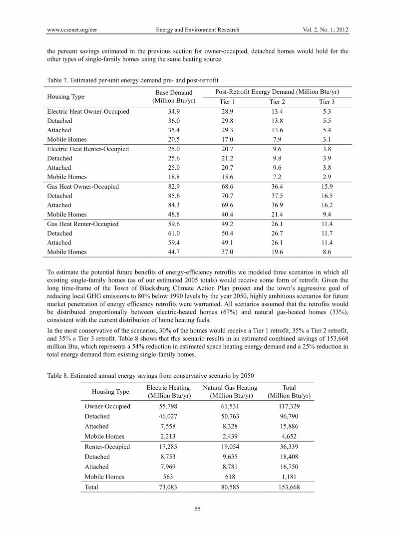
Table 7 compares the estimated baseline per-unit space heating energy demand (electric and gas heat) for all types of single-family homes to the resulting demand after each tier of retrofits. These calculations assume that


55

the percent savings estimated in the previous section for owner-occupied, detached homes would hold for the other types of single-family homes using the same heating source.

Table 7. Estimated per-unit energy demand pre- and post-retrofit

Housing Type Base Demand

(Million Btu/yr) Post-Retrofit Energy Demand (Million Btu/yr)

Tier 1 Tier 2 Tier 3

Electric Heat Owner-Occupied 34.9 28.9 13.4 5.3

Detached 36.0 29.8 13.8 5.5

Attached 35.4 29.3 13.6 5.4

Mobile Homes 20.5 17.0 7.9 3.1

Electric Heat Renter-Occupied 25.0 20.7 9.6 3.8

Detached 25.6 21.2 9.8 3.9

Attached 25.0 20.7 9.6 3.8

Mobile Homes 18.8 15.6 7.2 2.9

Gas Heat Owner-Occupied 82.9 68.6 36.4 15.9

Detached 85.6 70.7 37.5 16.5

Attached 84.3 69.6 36.9 16.2

Mobile Homes 48.8 40.4 21.4 9.4

Gas Heat Renter-Occupied 59.6 49.2 26.1 11.4

Detached 61.0 50.4 26.7 11.7

Attached 59.4 49.1 26.1 11.4

Mobile Homes 44.7 37.0 19.6 8.6

To estimate the potential future benefits of energy-efficiency retrofits we modeled three scenarios in which all existing single-family homes (as of our estimated 2005 totals) would receive some form of retrofit. Given the long time-frame of the Town of Blacksburg Climate Action Plan project and the town’s aggressive goal of reducing local GHG emissions to 80% below 1990 levels by the year 2050, highly ambitious scenarios for future market penetration of energy efficiency retrofits were warranted. All scenarios assumed that the retrofits would be distributed proportionally between electric-heated homes (67%) and natural gas-heated homes (33%), consistent with the current distribution of home heating fuels.

In the most conservative of the scenarios, 30% of the homes would receive a Tier 1 retrofit, 35% a Tier 2 retrofit, and 35% a Tier 3 retrofit. Table 8 shows that this scenario results in an estimated combined savings of 153,668 million Btu, which represents a 54% reduction in estimated space heating energy demand and a 25% reduction in total energy demand from existing single-family homes.

Table 8. Estimated annual energy savings from conservative scenario by 2050

Housing Type Electric Heating (Million Btu/yr)

Natural Gas Heating (Million Btu/yr)

Total (Million Btu/yr)

Owner-Occupied 55,798 61,531 117,329

Detached 46,027 50,763 96,790

Attached 7,558 8,328 15,886

Mobile Homes 2,213 2,439 4,652

Renter-Occupied 17,285 19,054 36,339

Detached 8,753 9,655 18,408

Attached 7,969 8,781 16,750

Mobile Homes 563 618 1,181

Total 73,083 80,585 153,668


56

The aggressive scenario, depicted in Table 9, shows the results of applying Tier 2 retrofits to 50% of existing homes and Tier 3 retrofits to the remaining 50%. This scenario reduces estimated space heating energy demand in those homes by 70% and total energy demand by 32%.

Table 9. Estimated annual energy savings from aggressive scenario by 2050




Owner-Occupied 72,398 79,290 151,688

Detached 59,720 65,415 125,135

Attached 9,806 10,732 20,538

Mobile Homes 2,872 3,143 6,015

Renter-Occupied 22,428 24,554 46,982

Detached 11,357 12,442 23,799

Attached 10,340 11,315 21,655


Total 94,825 103,844 198,669

Table 10 depicts the maximum scenario, in which 20% of homes receive a Tier 2 retrofit and 80% a Tier 3 retrofit. This scenario would result in a 78% reduction in space heating energy demand for existing single-family homes, and a 35% reduction in their total energy demand.

Table 10. Estimated annual energy savings from maximum scenario by 2050




Owner-Occupied 79,257 87,840 167,097

Detached 65,378 72,469 137,847

Attached 10,735 11,889 22,624

Mobile Homes 3,144 3,482 6,626

Renter-Occupied 24,552 27,202 51,754

Detached 12,434 13,784 26,218

Attached 11,320 12,536 23,856


Total 103,810 115,041 218,851

Figure 5 compares the results of the three retrofit scenarios to the baseline estimate of total space heating demand in single-family homes, showing that significant energy savings would be achieved in each scenario. In all cases total energy consumption from natural gas exceeds that from electricity, despite the fact that 2/3 of homes in Blacksburg use electric heat, because even the most basic electric heat pumps are approximately twice as efficient as natural gas furnaces.


57

Figure 5. Estimated energy demand from space heating after retrofits to existing single family homes

We converted these energy consumption savings into GHG using the afore-mentioned GHG emissions coefficients of 0.2078 metric tonnes CO2-e per million Btu of electricity consumption and 0.0532 tonnes/million Btu of natural gas. Figure 6 shows that the conservative scenario would reduce annual GHG emissions by 54%, from roughly 35,000 tonnes CO2-e to around 15,900. In the aggressive scenario these emissions would be reduced by 70% from the baseline, to about 10,300 tonnes, and in the maximum scenario they would drop 77%, to just over 8,000 tonnes.

Figure 6. Estimated GHG emissions from space heating after retrofits to existing single family homes

3. Addressing Challenges to Achieving Retrofit Savings

Despite their significant energy savings potential, four primary challenges limit the effectiveness of residential retrofits and the extent to which they are currently being implemented: methodological difficulties in estimating the potential of retrofits for multi-family units and for reducing air conditioning energy demand; the lack of incentive for retrofitting renter-occupied units; the lack of up-front financing for major retrofit projects; and a shortage of workers trained to conduct residential energy audits and retrofits. In Blacksburg, the town is collaborating with local and regional stakeholders to pursue creative solutions for addressing and overcoming these challenges.

0

50,000

100,000

150,000

200,000

250,000

300,000

350,000

Baseline Scenario 1 -Conservative

Scenario 2 -Aggressive

Scenario 3 -Maximum

Mill

ion

Btu

Natural Gas Electric

0

10,000

20,000

30,000

40,000

50,000

60,000

Baseline Scenario 1 -Conservative

Scenario 2 -Aggressive

Scenario 3 -Maximum

Ton

nes

CO

2-e

Natural Gas Electric


58

While single-family homes represent approximately ¾ of housing units nation-wide, and have greater energy-demand per-unit than multi-family units, achieving energy savings in existing multi-family buildings also will be necessary to reduce total residential energy use to acceptable levels over the coming years. This is particularly true for communities such as Blacksburg in which the percentage of multi-family units far exceeds the national average. Retrofits to multi-family units are promising due to their potentially smaller per-unit costs and payback periods as compared to a single family retrofit (Center for Neighborhood Technology, 2008). Unfortunately, while our models are accurate for estimating single-family home heating demand they have been less successful when adjusted for multi-family housing, in part because the internal heat gains from residents, appliances, etc. are much more difficult to estimate for an apartment building. Additionally, while residential retrofits have the potential to reduce cooling energy demand in the summer, little is known about the extent of these potential savings. Further research in these areas will help to further bolster the argument for local retrofit efforts.

The retrofitting of rental properties is also of particular importance in Blacksburg and other college towns, where they often represent more than half of all housing units. However, they present unique challenges for energy efficiency because there is little financial incentive for property owners to pay for improvements if their tenants will reap the benefit of reduced energy bills. The tenants also have little incentive to spend on efficiency improvements when they do not own the building and their tenure is likely to be less than the pay-back period of the investment. This conundrum is sometimes described as the “owner/tenant split financial incentive” (City of Berkeley, 2009, p. 68). One potential solution, recommended in the draft Blacksburg Climate Action Plan, is to create a voluntary energy efficiency rating and certification program for multi-family rental housing. The purpose of this program would be to identify energy-efficient rental units in the community, provide renters with information on the energy costs savings associated with those units, and thus allow property owners to charge a slightly higher rent in order to offset some of the costs of energy efficiency upgrades.

While the payback times for energy efficiency retrofits are generally favorable, many homeowners are challenged to come up with the several thousands of dollars in up-front costs that would be required for a substantial upgrade such as those modeled in our Tier 2 and Tier 3 retrofits. Therefore, one of the biggest challenges for local governments that wish to encourage residential energy efficiency is to identify creative ways to assist residents in financing the cost of a retrofit to their homes. In response to this challenge, local governments have adopted, or are considering, a variety of local financial incentives including grants or rebates for the purchase of energy-efficient products or materials, revolving loan programs, energy services contracts with on-bill financing, and property assessment clean energy (PACE) programs. The Town of Blacksburg, for example, has used the majority of its Energy Efficiency and Conservation Block Grant allocation to work in concert with a regional energy alliance called Community Alliance for Energy Efficiency (CAFE2) that coordinates a residential energy retrofit program. Blacksburg homeowners receive a rebate up to $500 to cover the cost of an initial energy audit if they follow through with the retrofit work, and a zero-interest loan up to $2,500 to cover a portion of the up-front cost of a building energy efficiency retrofit. CAFE2 is also working with the Federal Home Loan Bank to offer retrofit loans up to $15,000 to homeowners with less than 80% of median income for their locality. These loans are 20% forgiven each year, so that if homeowners stay in the residences for five years the entire loan is forgiven.

Although the art and science of building energy retrofit is well established, the availability of private sector vendors and trained evaluators to perform the retrofits is limited, and most homeowners do not know where to begin in determining the most effective use of their available resources to reduce their home energy costs. In response, Virginia Tech has piloted a residential energy education program (REEP) that trains students to provide free or nominal cost energy evaluations of residential houses. Although the students use some of the latest analytical tools for evaluation, including blower doors, duct blasters, infrared cameras, and electrical submeters, the evaluations are not billed as a full professional energy audit. They do, however, identify opportunities for efficiency improvements to the building envelope, HVAC equipment, appliances, and lighting, along with recommendations for further audit work and retrofit measures by private vendors.

Finally, as with many local energy and GHG emission reduction opportunities, residential retrofit programs will likely be more effective if they expand beyond the boundaries of a given municipality and provide consistent support for homeowners across a given metropolitan area or region. For example, as mentioned above, the Town of Blacksburg has partnered with neighboring jurisdictions in the CAFE2 energy alliance, which provides a consistent approach to residential retrofits and increases the opportunities for the region to receive state and federal funding for these initiatives.

4. Conclusions

These findings demonstrate the potential for energy-efficiency retrofits to significantly reduce energy demand in


59

single-family homes. The “tiers” of retrofits we modeled show that even a basic upgrade of windows and ceiling insulation reduces predicted space heating demand by 17%, while an aggressive retrofit using the best available technologies could reduce that demand by more than 80%. Actual energy savings from a “real-life” retrofit would fall somewhere in between these two totals, depending on the extent of the retrofit and the amount the home-owner is willing to spend on top-of-the-line insulation and HVAC systems.

The three scenarios for future retrofits demonstrate potential community-wide savings from a concentrated effort to improve existing housing stock. It must be noted, however, that this study does not take into account the “rebound effect”, or the potential for some of the energy savings to be offset by behavior changes such raising thermostat temperatures to increase thermal comfort. Lloyd (2008) cites several previous European studies that found actual energy savings from retrofit programs to be lower than expected due to this effect, with the general consensus being that lower-income households will primarily experience thermal comfort improvements, while reduced energy consumption would take place primarily in higher-income households. Even without factoring in the rebound effect, these savings translate to reductions of no more than 36% (aggressive scenario) in total projected residential energy demand for the year 2050. Clearly, reducing overall residential energy consumption to the extent necessary to achieve Blacksburg’s aggressive GHG reduction goals will also require aggressive energy efficiency measures for new homes, water heating and appliances (in both new and existing homes), and solar PV or other forms of on-site renewable energy.

Nevertheless, the potential savings are significant enough, and realistic enough, to merit a full-scale effort to retrofit existing homes as part of local climate action planning initiatives. It is again important to note that these scenarios are extremely ambitious, as they were prepared in the context of a community climate action plan with a 40-year planning horizon and a goal of reducing local GHG emissions to 80% below 1990 levels by the year 2050. Such savings could only be achieved in the real world through a dramatic, concerted, community-wide effort to retrofit homes on a large scale, which would require substantial financial incentives and other policy directives. However, this same methodology could be used to model scenarios for more modest changes in the short-term, such as those that might be gained from a specific local policy like providing a set amount of zero-interest loans for energy efficiency retrofits.

Acknowledgements

This research was made possible by a grant from the Town of Blacksburg. The authors would like to thank Susan Garrison and Kelly Mattingly at the Town of Blacksburg Public Works Department for their support and guidance on this project, along with the following individuals who provided useful feedback and advice: Sean McGinnis, David Roper, Bill Claus, Joe Mugavero, and Chase Counts.

References

Bailey, J. (2007). Lessons from the Pioneers: Tackling Global Warming at the Local Level. Minneapolis, MN: Institute for Local Self Reliance.

Bassett, E., & Shandas, V. (2010). Innovation and climate action planning: perspectives from municipal plans. Journal of the American Planning Association, 76(4), 435-450. http://dx.doi.org/10.1080/01944363.2010.509703

Betsill, M. (2001). Mitigating climate change in US cities: opportunities and obstacles. Local Environment, 6(4), 393-406. http://dx.doi.org/10.1080/13549830120091699

Brown, M., & Berry, L. (1993). Weatherization Assistance: the Single-Family Study. Retrieved from http://www.homeenergy.org/archive/hem.dis.anl.gov/eehem/93/930907.html (January 8, 2009)

Brown, M., & Logan, E. (2008). The residential energy and carbon footprints of the 100 largest U.S. metropolitan areas. Georgia Institute of Technology. Retrieved from http://www.spp.gatech.edu/faculty/workingpapers/wp39.pdf (March 1, 2011)

Center for Neighborhood Technology. (2008). Chicago Greenhouse Gas Emissions: An Inventory, Forecast, and Mitigation Analysis for Chicago and the Metropolitan Region. Retrieved from http://www.chicagoclimateaction.org/filebin/pdf/FINALALL091708_1-118.pdf (October 1, 2011)

Choi Granade, H., Creyts, J., Derkach, A., Farese, P., Nyquist, S., & Ostrowski, K. (2009). Unlocking Energy Efficiency in the U.S. Economy. McKinsey and Company. Retrieved from http://ww1.mckinsey.com/clientservice/ccsi/pdf/US_energy_efficiency_full_report.pdf (February 1 2009)

City of Berkeley. (2009). Berkeley Climate Action Plan. Retrieved from http://www.berkeleyclimateaction.org/docManager/1000000266/BCAP%20Chapters.pdf (July 1, 2010)


60

City of Berkeley. (2011). RECO: Compliance Steps for Sale or Transfer of Property. Retrieved from http://www.ci.berkeley.ca.us/ContentDisplay.aspx?id=19562 (May 1, 2011)

City of Boulder. (2006). Climate Action Plan. Retrieved from http://www.bouldercolorado.gov/files/Environmen tal%20Affairs/climate%20and%20energy/cap_final_25sept06.pdf (July 1, 2010)

City of Portland. (2011). Clean Energy Works Portland. Retrieved from http://www.portlandonline.com/bps/index.cfm?c=50152& (May 1, 2011)

City of San Francisco. (2009). What You Should Know about San Francisco’s Residential Energy and Water Conservation Requirements. Retrieved from http://www.sfdbi.org/Modules/ShowDocument.aspx?documen tid=124 (May 1, 2011)

Cohen, S., Goldman, C., & Harris, J. (1991). Energy savings and economics of retrofitting single-family buildings. Energy and Buildings, 17(4), 297-311. http://dx.doi.org/10.1016/0378-7788(91)90012-R

Dineen, D., & Ó Gallachóir, B. P. (2011). Modelling the impacts of building regulations and a property bubble on residential space and water heating. Energy and Buildings, 43(1), 166-178. http://dx.doi.org/10.1016/j.enbuild.2010.09.004

Energy Center of Wisconsin. (2011). National Weatherization Assistance Program Evaluation. Retrieved from http://www.ecw.org/weatherization/background.php (May 1, 2011)

Ewing, R., & Rong, F. (2008). The impact of urban form on residential energy use. Housing Policy Debate, 19(1), 1-30. http://dx.doi.org/10.1080/10511482.2008.9521624

Goldman, C. (1985). Measured energy savings from residential retrofits: updated results from the BECA-B project. Energy and Buildings, 8(2), 137-155. http://dx.doi.org/10.1016/0378-7788(85)90022-2

Hens, H., Verbeek, G., & Verdonck, B. (2001). Impact of energy efficiency measures on the CO2 emissions in the residential sector, a large scale analysis. Energy and Buildings, 33(3), 275-281. http://dx.doi.org/10.1016/S0378-7788(00)00092-X

Hirst, E., & Goeltz, R. (1985). Estimating energy savings due to conservation programmes: The BPA residential weatherization pilot programme. Energy Economics, 7(1), 20-28. http://dx.doi.org/10.1016/0140-9883(85)90035-0

Kaza, N. (2010). Understanding the spectrum of residential energy consumption: a quantile regression approach. Energy Policy, 38(11), 6574-6585. http://dx.doi.org/10.1016/j.enpol.2010.06.028

Lloyd, C. R., Callau, M. F., Bishop, T., & Smith, I. J. (2008). The efficacy of an energy efficient upgrade program in New Zealand. Energy and Buildings, 40(7), 1228-1239. http://dx.doi.org/10.1016/j.enbuild.2007.11.006

Moomaw, W., & Johnston, L. (2008). Emissions mitigation opportunities and practice in Northeastern United States. Mitigation and Adaptation Strategies for Global Change, 13(5-6), 615-642. http://dx.doi.org/10.1007/s11027-007-9135-0

Oak Ridge National Laboratory. (2010). Insulation Fact Sheet. Retrieved from http://www.ornl.gov/sci/roofs+walls/insulation/ins_16.html (July 1, 2010)

Parker, P., Rowlands, I. H., & Scott, D. (2005). Who changes consumption following residential energy evaluations? Local programs need all income groups to achieve Kyoto targets. Local Environment, 10(2), 173-187. http://dx.doi.org/10.1080/1354983052000330761

Philadelphia Housing Development Corporation. (2010). 2010 Annual Report. Retrieved from http://www.phdchousing.org/reports/PHDC%20Annual%20Report%202010%20for%20web.pdf (May 1, 2011)

Pitt, D, & Randolph, J. (2009). Identifying Obstacles to Municipal Climate Protection Planning. Environment and Planning C: Government and Policy, 27(6), 841-857. http://dx.doi.org/10.1068/c0871

Pratt Center for Community Development. (2011). Retrofit NYC Block by Block. Retrieved from http://prattcenter.net/retrofit-nyc-block-block (May 1, 2011)

Randolph, J. (2008). Comment on Reid Ewing and Fang Rong's “The impact of urban form on residential energy use.” Housing Policy Debate, 19(1), 45-52. http://dx.doi.org/10.1080/10511482.2008.9521626

Randolph, J., Greely, K., & Hill W. (1991). Evaluation of Virginia Weatherization Program. Blacksburg, VA: Virginia Center for Coal and Energy Research.


61

Randolph, J., & Masters, G. (2008). Energy for Sustainability: Technology, Planning, Policy. Washington DC: Island Press.

Schneiders, J. (2003). CEPHEUS – Measurement Results from More than 100 Dwelling Units in Passive Houses. Passive House Institute, Darmstadt, Germany. Retrieved from http://www.eceee.org/conference_proceedings/eceee/2003c/Panel_2/2047schnieders (May 1, 2011)

Schweitzer, M. (2005). Estimating the National Effects of the U.S. Department of Energy’s Weatherization Assistance Program with State-Level Data: A Metaevaluation Using Studies from 1993 to 2005. Retrieved from http://weatherization.ornl.gov/pdfs/ORNL_CON-493.pdf (May 1, 2011)

Seattle City Light. (2011). 2008-2012 Action Plan: Conservation Resources Division. Retrieved from http://www.seattle.gov/light/conserve/docs/Conservation_5_Year_Action_Plan.pdf (May 1, 2011)

U.S. Census Bureau. (2000). Census 2000. Retrieved from http://factfinder.census.gov/servlet/DatasetMainPage Servlet?_program=DEC&_submenuId=datasets_2&_lang=en&_t (November 1, 2009)

U.S. Census Bureau. (2008). 2006-2008 American Community Survey 3-Year Estimates. Retrieved from http://factfinder.census.gov/servlet/DatasetMainPageServlet?_program=ACS&_submenuId=datasets_2&_lang=en (November 1, 2009)

U.S. Census Bureau. (2010). 2006-2010 American Community Survey 5-Year Estimates. Retrieved from http://factfinder2.census.gov/faces/nav/jsf/pages/searchresults.xhtml?refresh=t (February 19, 2011)

U.S. Council on Environmental Quality. (2009). Recovery through Retrofit. Retrieved from http://www.whitehou se.gov/assets/documents/Recovery_Through_Retrofit_Final_Report.pdf (February 28, 2011)

U.S. Department of Energy. (2005). Residential Energy Consumption Survey. Table US14. Retrieved from http://www.eia.doe.gov/emeu/recs (November 1, 2009)

U.S. Department of Energy. (2007). Instructions for Form EIA-1605: Voluntary reporting of greenhouse gases. Retrieved from http://www.eia.doe.gov/oiaf/1605/pdf/Form%20EIA-1605%20Instructions.pdf (May 2, 2011)

U.S. Department of Energy. (2009). American Recovery and Reinvestment Act. Retrieved from http://www1.eere.energy.gov/recovery/(October 1, 2010)

U.S. Department of Energy. (2010a). Annual Energy Review, Energy Consumption by Sector, 1949-2009. Retrieved from http://www.eia.doe.gov/emeu/aer/consump.html (July 1, 2010)

U.S. Department of Energy. (2010b). Accelerating Adoption of Energy Efficiency and Renewable Energy. Retrieved from http://www1.eere.energy.gov/wip/pdfs/wip_factsheet.pdf (July 1, 2010)

U.S. Department of Energy. (2010c). Review of Selected Home Energy Auditing Tools: In Support of the Development of a National Building Performance Assessment and Rating Program. Prepared by Sentech Inc. for the U.S. Department of Energy. Retrieved from http://apps1.eere.energy.gov/buildings/publications /pdfs/homescore/auditing_tool_review.pdf (December 1, 2011)

U.S. Department of Energy. (2010d). Overview of Existing Home Energy Labels.Navigant Consulting for the U.S. Department of Energy. Retrieved from http://apps1.eere.energy.gov/buildings/publications/pdfs/homescore/existing_labels.pdf (December 1, 2011)

U.S. Department of Energy. (2011). Home Energy Score. Retrieved from http://www1.eere.energy.gov/buildings/homeenergyscore (December 1, 2011)

U.S. Environmental Protection Agency. (2010). E-Grid2010 Version 1.0, Year 2007 Summary Tables. Retrieved from http://www.epa.gov/cleanenergy/energy-resources/egrid/index.html (May 1, 2011)

Verbeeck, G., & Hens, H. (2005). Energy savings in retrofitted dwellings: economically viable. Energy and Buildings, 37(7), 747-754. http://dx.doi.org/10.1016/j.enbuild.2004.10.003

Wall, L., Goldman, C., & Rosenfeld, A. (1983). Building energy use compilation and analysis (BECA).Part B: Retrofit of existing North American residential buildings. Energy and Buildings, 5(3), 151-170. http://dx.doi.org/10.1016/0378-7788(83)90003-8

Yalcintas, M., & Kaya, A. (2009). Conservation vs. renewable energy: Cases studies from Hawaii. Energy Policy, 37(8), 3268–3273. http://dx.doi.org/10.1016/j.enpol.2009.04.029

estimating potential community-wide energy and greenhouse gas

Documents