Estimating Natural Gas Salt Cavern Storage

Costs

Nathalie HincheyGraduate Student

Center for Energy StudiesJames A. Baker III Institute for Public Policy

Rice University6100 Main StreetHouston, Texas

77005USA

nh17@rice.edu

Abstract

Peak load natural gas storage demand is primarily served from saltcaverns as they offer high deliverability, with both injection and with-drawal rates easy to vary on short notice. Many short term traders usesalt cavern storage to maximize profits by arbitraging differences in pricefrom unpredictable and occasionally unanticipated demand surges. It isgenerally acknowledged that higher storage levels increase injection costsand reduce withdrawal costs. Recently, there has been a dearth of in-vestment in new gas storage capacity. Forecasts, however, predict thatdemand for storage capacity in the Gulf Region will increase in the nextfew years, mainly in response to US LNG exports and the use of naturalgas in power generation. LNG exports, in particular, will likely increaseseasonality in demand for U.S. natural gas since the primary importersof U.S. natural gas, Europe and Asia, have less storage themselves. Thisdemand will put pressure on existing storage capacity. Comprehensionas to how storage, injection and withdrawal costs respond to increaseddemand for storage is essential to understanding natural gas pricing.

1

1 Introduction

Natural gas is an important fuel source used for residential heating, industrial

manufacturing, and power generation in the U.S. and many other countries. It is

the cleanest fossil fuel and provides significant additional advantages for power

generation due to its widespread availability, dispatchability and affordability.

A significant challenge for the natural gas sector, however, is the seasonal and

volatile nature of demand paired with the steady and constant nature of its

supply. In months with extreme temperatures, demand for natural gas skyrock-

ets, while in temperate months demand decreases significantly. This leads to

unattractive price volatility for purchasers of natural gas and potential profits

for owners if natural gas storage facilities, who can take advantage of spatial

and intertemporal arbitrage opportunities. Storing natural gas during times of

low demand and prices and increasing supply by drawing down inventories dur-

ing times of high demand and prices also assists consumers by decreasing price

variation. Storage of natural gas also helps transmission companies manage

sudden load variations and maintain system stability. More widespread use of

natural gas storage depends on its cost. In this paper, I use a GMM estimation

technique on first order conditions from a structural model of a representative

agent to investigate the operating costs of salt cavern storage facilities.

Prior to 1992, gas storage facilities were almost exclusively owned and con-

trolled by interstate and intrastate pipeline companies. They sold natural gas to

consumers as a bundled service including production, transmission and storage

services. In April 1992, the Federal Energy Regulatory Commission (FERC)

issued Order 636, which essentially unbundled these services to help foster the

structural changes necessary to create a competitive market for the American

natural gas industry (American Gas Association, 2017). Order 636 instructed

owners of storage facilities to open access to storage to third parties and only

2

allowed the former to reserve space for their own use to balance system supply.

The newly deregulated market presented new arbitrage opportunities. Previ-

ously, storage could be used only as a physical hedge to market conditions.

After liberalization, it could also be used a financial tool to profit from price

differentials for short term gas traders (Schoppe, 2010). Order 636, along with

high price volatility, led to an impressive expansion of high deliverability storage

facilities during the late nineteen nineties (Fang et al., 2016). High deliverabil-

ity facilities allow for rapid injection and withdrawal of gas from storage, but

generally tend to have lower storage capacity. They are especially important for

supplying unexpected demand surges in the electricity generation sector.

In 2016, as in the three preceding years, no new underground facilities were

developed in the U.S. and the only expansion of capacity has been represented by

brownfield investment in the South Central (Gulf) region, concentrated mostly

in high deliverability salt cavern storage facilities (EIA, 2017b).

The nature of natural gas demand also has been changing and will continue to

do so. Overall, demand changes can be attributed to three main causes. First,

natural gas use for power generation has grown substantially in recent years

and is expected to grow further not only because of the relatively high energy

efficiency and low cost of combined cycle natural gas plants. Single cycle natural

gas turbines are also a good complement to intermittent renewable generation

sources. Second, industrial demand for natural gas has been growing in recent

years, although this demand growth contributes to base load demand. Third,

LNG exports are expected to strengthen the demand for U.S. gas with the U.S.

expected to become a net gas exporter in 2017 (EIA, 2017c). The importance of

these sources of natural gas demand will put a premium on gas storage facilities

that can meet sudden demand surges. Understanding the effects these changes

will have on natural gas storage facilities is then of great importance.

3

To understand the demand for storage facilities, a comprehensive analysis

that considers regional responses to demand and supply changes is needed. A

recent study by Fang et al. (2016) uses a proprietary nonlinear programming

system to model the U.S. natural gas market. They examine how gas stor-

age utilization will be affected under two different scenarios. In a base case

scenario, wide availability of natural gas lead to increases in power sector de-

mand and LNG exports. In a contrasting “Low Oil and Gas Resource” case,

renewable energy becomes more prominent in the power sector and natural gas

generation is used only to stabilize the system. At an aggregate level, the study

finds there will be very little additional storage needed under either case. The

study also predicts, however, that higher LNG exports and increased demand

for natural gas in the power sector will increase utilization of high deliverability

storage in the Gulf region, which mainly takes the form of salt cavern storage

facilities.Nevertheless, the study does not find that storage expansion will be

warranted, implying that existing salt cavern storage facilities will be stressed.

The costs of injecting and withdrawing natural gas from salt caverns, and re-

sponses and reactions to increased utilization of such facilities, will therefore

likely have an increasing impact on natural gas prices and stability of the nat-

ural gas delivery system.

Industry experts suggested, anecdotally, that the cost of injecting/withdrawing

natural gas from storage depends on both the level of gas stored in the facility

and the rate of injection/withdrawal. In particular, costs of injecting natural

gas appear relatively stable and constant when inventory levels are below 85%-

90% of total storage capacity, but increase at an increasing rate when storage

levels exceed this threshold. Similarly, withdrawal costs escalate when storage

levels near the minimum (cushion gas) level. Figure 1 illustrates these effects of

storage levels on injection and withdrawal costs.

4

Spare Capacity in Storage

Injection Cost

(a) Injection Costs as Storage Levels Change

Storage Level

Withdrawal Cost

(b) Withdrawal Costs as Storage Levels Change

Figure 1: Injection and Withdrawal Costs

5

It has been observed that as utilization in salt cavern storage facilities in-

crease, a higher inventory level (or cushion gas) is required to maintain the

integrity of the facility (FERC, 2004). Increased utilization in the Gulf region

will therefore most likely increase the injection costs into storage for salt cavern

storage facilities.

The main contribution of this paper will be to examine what would happen

to injection costs if storage utilization in the Gulf region increased due to LNG

exports and enhanced demand from the power sector. Specifically, the primary

goal will be to develop and estimate a model that quantifies the degree to which

injection costs increase when storage levels near capacity. There are a number

of benefits of estimating such a cost function: it will aid in valuation of gas

storage methodologies; it will provide more clarity on the pricing of natural gas;

and it will give some insight into the behavior of short term gas traders.

To facilitate the understanding of this problem, the next section will present

a brief introduction on the different types of demand for natural gas storage,

the physical properties and types of underground storage, and the nature of

gas storage contracts. The paper will then provide a literature review of the

relevant research in this area, which will be followed by the theoretical model

and model estimation, and finally an analysis of future expected storage costs.

2 Types of Demand for Natural Gas Storage

Due to its gaseous state, natural gas needs to be stored in an environment that

pressure low enough to limit leakage and resulting losses of the fuel. On the

other hand, pressure in the storage facility assists the extraction of gas from

storage. Naturally occurring underground formations, such as depleted oil and

gas reservoirs, aquifers and salt caverns provide the most effective means to store

6

gas in its natural form. Alternatively, natural gas can be stored in pipelines

(when spare capacity is available) or as LNG1 in LNG storage tanks. The latter

requires liquefaction of the fuel prior to storage and regasification before it can

be injected back into a pipeline system. Each type of storage facility has its own

set of physical properties, which in turn determine the cost of storing natural

gas as well as the type of storage that the facility is best suited for.

In principal, there are two different purposes for storing natural gas. The

first is to meet predictable seasonal variations in natural gas demand. Storage

operators purchase natural gas during times of low demand, or the “shoulder

months”,2 and sell the gas during periods of high demand, in order to arbitrage

profitable seasonal price differences. Typically, natural gas demand is highest

during the winter months when it is used to heat houses, commercial and indus-

trial interiors. Increasingly, natural gas is also used during the summer months

to provide air conditioning, as natural gas open cycle turbines provide most of

the peaking power generation in the United States. In 2016, natural gas ac-

counted for approximately 33.8% of electric generation in utility scale facilities

(EIA, 2017), although an increasing number of these would be combined cycle

plants used to provide base or intermediate load, which tend to be less sea-

sonal in nature. It is the predictable, seasonal nature of demand for natural gas

that has provided the need and incentive to develop storage facilities. Figure

2 illustrates the seasonal demand for natural gas. Natural gas stored to meet

predictable seasonal variations in demand tends to be held in storage for longer

periods to account for changing seasons and weather patterns.

Natural gas storage can also be used to meet unpredicatable peak load de-

1Liquefied Natural Gas (LNG) is obtained by cooling natural gas (in a liquefaction plant)to -260 degrees Fahrenheit, (-162.2 degrees Celsius), after the extraction of oxygen, waterand carbon dioxide, as well as most sulfates (Office of Fossil Energy, 2016). This reduces thevolume by a factor of 600 and permits cost-effective transport by way of specially constructedtanker ships. A regasification plant turns the LNG back into natural gas after delivery.

2These are generally the months of May-June and September-October.

7

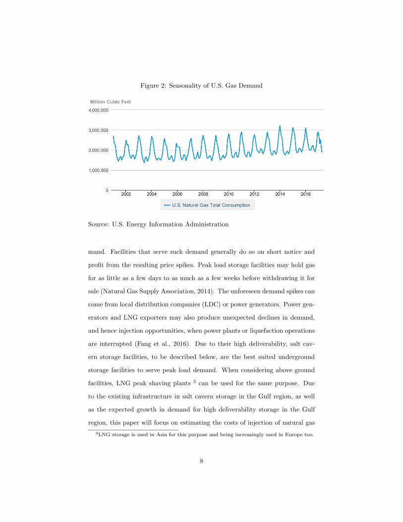
Figure 2: Seasonality of U.S. Gas Demand

Source: U.S. Energy Information Administration

mand. Facilities that serve such demand generally do so on short notice and

profit from the resulting price spikes. Peak load storage facilities may hold gas

for as little as a few days to as much as a few weeks before withdrawing it for

sale (Natural Gas Supply Association, 2014). The unforeseen demand spikes can

come from local distribution companies (LDC) or power generators. Power gen-

erators and LNG exporters may also produce unexpected declines in demand,

and hence injection opportunities, when power plants or liquefaction operations

are interrupted (Fang et al., 2016). Due to their high deliverability, salt cav-

ern storage facilities, to be described below, are the best suited underground

storage facilities to serve peak load demand. When considering above ground

facilities, LNG peak shaving plants 3 can be used for the same purpose. Due

to the existing infrastructure in salt cavern storage in the Gulf region, as well

as the expected growth in demand for high deliverability storage in the Gulf

region, this paper will focus on estimating the costs of injection of natural gas

3LNG storage is used in Asia for this purpose and being increasingly used in Europe too.

8

into salt caverns in the Gulf region.

3 Physical Properties and Types of Underground

Storage

Depleted oil and gas reservoirs, aquifers, and salt caverns are the most common

formations used for underground storage. The particular desirability of these

three types of underground storage is based on their geological and geographical

traits. Each differs in terms of its working gas capacity, base (cushion) gas,

shrinkage factor, deliverability and geographical location. A storage facility’s

working gas capacity refers to the amount of gas that can be injected into

and withdrawn from storage for use. Since storage reservoirs must maintain a

certain amount of pressure for extraction purposes, there is a minimum amount

of gas required, called the base or cushion gas level, below which no gas can

be extracted from storage. Essentially, a storage operator must inject a certain

amount of gas into the reservoir that is extremely difficult to recover. It is more

profitable to have a lower base gas level. The working gas capacity and the base

gas make up the total capacity of storage.

The shrinkage factor of a storage facility refers to the amount of leakage of

gas that occurs from the reservoir. All underground facilities lose some natural

gas through leakage, with the amount lost depending on the permeability if the

encloding rock and pressure. Deliverability reflects the rate at which gas can be

withdrawn from and injected into storage. Higher deliverability indicates that

natural gas can be cycled through the storage site more quickly. Finally, the

proximity of the storage site to end users and market centers affects the price of

the stored gas and the value of the facility for meeting peak demand changes.

Brief descriptions of the aforementioned types of storage facilities are presented

9

below.

3.1 Depleted Oil and Gas Reservoirs

Depleted oil and gas reservoirs consist of underground formations that have in-

creased pore space as a result of prior oil and gas extraction. These formations

provide natural cost advantages as the geological characteristics of the site are

already known from previous activity. Further, depleted reservoirs normally

have existing infrastructure to extract and transport natural gas, which lowers

investment costs. The surrounding rock is also often non-porous (the reason the

hydrocarbons were trapped in the fisrt place), which reduces leakage. Conse-

quently, depleted reservoirs are generally the cheapest storage sites to develop

and are the most abundant type of storage in the United States. They are pri-

marily located in producing regions of the U.S. and require about 50% base gas

(Natural Gas Supply Association, 2014). Depleted reservoirs are typically used

to satisfy base load demand as they have lower deliverability.

3.2 Aquifers

Natural aquifers can also be converted for use as a natural gas storage site. They

have geological characteristics similar to depleted reservoirs (EIA, 2015b), yet

they are less well known. Essentially, the natural gas displaces water instead

of hydrocarbons from the pore spaces in the rock. Aquifers are generally more

expensive to develop than depleted reservoirs and require the highest base gas

of all 3 storage facility types. They are generally used for base load demand,

although they are occasionally employed to serve peak load demand as well

(Natural Gas Supply Association, 2014). Aquifers are the least desirable form

of storage and are generally commissioned when there are no depleted fields or

salt caverns nearby.

10

3.3 Salt Caverns

Salt caverns are primarily located in the Gulf region and are created by a process

called “salt mining” where water is injected into salt formations underground

to dissolve the salt and create a cavern (Fairway Energy, 2017). While salt

caverns require the highest initial investments for development, they provide

the lowest per unit costs for gas storage. This is due to the high deliverability

of salt caverns, which is higher than both depleted reservoirs and aquifers. Salt

caverns only require about 33% of cushion gas (Fang et al., 2016) but have

much lower storage capacity. Since this makes them less viable to serve base

load demand, they are primarily employed to serve peak load demand. They

account for approximately 10% of working storage capacity in the U.S.4 and

28% of daily deliverability (EIA, 2015a).

4 Storage Technology and Contracts

When the owners of natural gas decide to inject or withdraw gas from storage,

they are motivated primarily by anticipated price differences compared to their

variable costs, which in turn equal the sum of the injection and withdrawal

prices charged by storage operators. Understanding the nature of storage con-

tracts is then vital to modeling the decision of natural gas owners to inject and

withdraw gas from storage. We will later use these decisions to help uncover

their respective cost functions.

The majority of underground natural gas storage facilities are owned by

interstate and intrastate pipeline transmission companies, although a significant

number are owned by LDCs and independent storage operators as well (Natural

Gas Supply Association, 2014). Owners of storage facilities generally lease out

storage space to third party clients according to detailed contracts that specify

4Specifically, in the lower 48 States.

11

a monthly, fixed payment based on the leased storage space, as well as variable

payments. The monthly leasing rate depends on the type of service required by

the customer. A renter can either choose to purchase uninterruptible service,

which guarantees access to the allocated storage space, or interruptible service,

where the rented space is accessible only when the storage provider is capable of

providing the space. Predictably, uninterruptible space is more expensive than

interruptible storage space.

The storage operator also charges for injecting natural gas into, and with-

drawing natural gas out of, storage, including associated fuel costs. The oper-

ator may also impose daily withdrawal and injection limits. Since extraction

and injection use different technologies, the injection and extraction costs typi-

cally, but not always, are not identical. In fact, the Spindletop storage facility

in Beaumont, Texas, operated by Centana Intrastate, which will be examined

in this paper, charges the same rate5 to inject and extract natural gas, within

daily maximum injection and withdrawal bounds.

To inject natural gas into storage, the incoming gas needs to be filtered

and then compressed by a gas motor or turbine, which requires fuel (DEA,

2017). Most natural gas contracts, according to postings by the Texas Railroad

Commission, charge approximately 2% of injected gas volume to cover fuel costs,

in addition to the injection charge.

To extract natural gas from storage, the gas first needs to be sufficiently

pressurized. Compressors may be required to compress the gas before it is

injected into the pipeline network. While in storage, gas absorbs water which

can be corrosive and damaging to pipelines. Storage operators must thus remove

all hydrates from the gas, usually through a process called glycol dehydration

(DEA, 2017).

5Based on the most recent rate postings by the Texas Railroad Commission.

12

5 Literature Review

There appears to be no, or a negligible amount, of research on estimating storage

injection/withdrawal costs. This may be because data on costs and storage

levels are needed and are either not readily available or are available only at

the aggregate level. Most research analyzing underground natural gas storage

has focused on valuing underground storage fields. Most of the literature uses

either intrinsic valuation methods, which essentially value storage facilities using

seasonal price spreads, or extrinsic valuation techniques, which focus on financial

hedging and trading. All of the papers described in this section use calibration

techniques to place a value on storage. As far as we know, this is the first paper

to estimate a model of the natural gas and storage problem.

Boogert and De Jong (2008) develop a Monte Carlo valuation method where

they employ a Least Squares Monte Carlo methodology using an American op-

tions framework to model the investment decisions of storage and ultimately

value storage. Cortes (2010) expands this methodology by introducing multi-

factor processes into the Least Squares Monte Carlo algorithm. Chen and

Forsyth (2007), on the other hand, develop a valuation method using a semi-

Lagrangian technique to solve the storage problem that is modeled as a Hamilton-

Jacobi-Bellman equation. Thompson et al. (2009) derive a valuation method us-

ing nonlinear partial-integro-differential equations. Finally, Henaff et al. (2013)

and Li (2007) both present valuation methods that effectively combine extrinsic

and intrinsic valuation principals to represent a more realistic setting.

These papers do not focus on the cost of injecting and withdrawing natural

gas into and from storage respectively, nor how these costs change with storage

levels. These costs will ultimately affect profitability and should be expected

to influence the final calibrated valuations of underground natural gas storage.

The results from this paper should be helpful in increasing the reliability of the

13

valuation methodologies described above.

The storage decision problem can also be viewed as an inventory problem,

and many papers have examined the decision to invest in inventories. This

paper uses an empirical approach very similar to the Euler-equation estimation

technique, first introduced by Hansen and Singleton (1982). In the context of

this paper, the most important research on the inventory problem was performed

by Cooper et al. (2010). While looking at the decision to invest in capital,

Cooper et al. (2010) use Euler equations to recover capital investment costs in

a discrete choice setting with periods of inactivity. The methodology employed

in Cooper et al. (2010) is very similar to the estimation technique proposed in

this paper to estimate natural gas injection costs.

6 Data

Proprietary data on the injection and withdrawal rates of gas into the Spindletop

Storage Facility, operated by Centana Intrastate, was generously provided by

Genscape, Incorporated. The Spindletop storage facility is a salt cavern storage

field located in Jefferson County, Texas with a storage capacity of 21,100 million

cubic feet (Mmcf) and cushion gas of 6929.8 Mmcf. It has similar characteris-

tics to most other salt cavern storage facilities in the Gulf region. Genscape,

Inc. monitors gas flows into and out of storage using infrared technology and

electro-magnetic field monitors. Daily storage levels and rates are measured in

Mmcf and are observed from June 1, 2015 to January 31, 2017. Of note is that

the data set has observations of storage levels that exceed 85% of storage ca-

pacity whereas it has no observations that are near cushion gas levels. This will

make identifying the asymptotic nature of withdrawal costs, when inventories

approach cushion gas levels, impossible. The rest of the paper will therefore

focus on estimating the injection cost function.

14

The gas trading hub located nearest the Spindletop storage cavern is the

NGPL Texas Oklahoma (TexOk) Gas Trading Hub. Daily TexOk spot prices

were obtained from Bloomberg. Since the futures prices at TexOk were not

readily available, I constructed the TexOk futures prices by determining the

differential between the TexOk and Henry Hub spot prices and adjusting the

Henry Hub futures prices with the differential between the TexOk and Henry

Hub spot prices. Prices on the weekends were filled with Friday’s prices since

injection and withdrawal activity were observed on the weekends.

The operating characteristics of the Spindletop Facility, such as working

gas capacity and base gas, measured in Mmcf, were obtained from the Texas

Railroad Commission. Since prices are reported in $/Mmbtu and the operating

characteristics as well as the injection/withdrawal rates were given in Mmcf,

the gas quantities in the dataset were converted to Mmbtu by multiplying these

values by a factor of 1037 (EIA, 2017d) to provide consistent units.

7 Model and Results

7.1 Theoretical Model

We build a model where a representative agent in a competitive natural gas mar-

ket maximizes expected profits by making a series of investment decisions based

on storage volumes, spot prices and futures prices. Let pst,T represent the spot

price of natural gas on day t in month T and Ft,T (n) denote the futures price

on day t in month T for delivery in month T + n at the trading hub. Contracts

expire at the TexOk Trading Hub on the last business day of the month. Define

it,T as the amount of gas injected into, (it,T > 0), or withdrawn from, (it,T < 0),

storage at time t and month T . Allow SMax to be the maximum storage ca-

pacity, and SMin the base gas (cushion gas), of the storage facility. Let St,T

15

represent the level of gas in storage on day t in month T . CI(St−1,T , it,T , SMax)

is the cost of injecting it,T gas into storage, which is a function of the previous

end of day storage level, St−1,T , and the maximum storage capacity, SMax,

as well as the injection rate, it,T . The domain of CI(St−1,T , it,T , SMax) is

(St−1,T , it,T , SMax) ∈ [Smin, SMax] × [0, SMax − St−1,T ] × R++. The cost of

withdrawing gas, CW (it,T ), is only a function of the amount of gas withdrawn,

it,T , for it,T negative. Specifically, the domain of CW (it,T ) is [SMin−St−1,T , 0].

The withdrawal cost function is not modeled to be dependent on inventory lev-

els because, as discussed in the following section, such a function cannot be

identified in the data set. Let CFuel(it,T ) represent the variable fuel cost in-

curred during injection. The function CFuel(it,T ) is defined to be 0 when it,T is

negative and some increasing function of it,T when it,T is positive. Let NT be

the number of days in month T . Finally, define the agent’s information set on

day t in month T as It,T and β as the daily discount factor.

The profit maximizing agent then solves the following problem:

maxit,T∈Γt,T

E

[∑T

[NT−1∑t

βt+∑T−1i=0 Ni

((Ft,T (1)− pSt,T )it,T

− 1{it,T > 0}[CI(St−1,T , it,T , SMax) + CFuel(it,T )]

− 1{it,T < 0}CW (it,T )

)+ βNT+

∑T−1i=0 Ni

((pSNT ,T − FNT ,T (1))SNT ,T + (FNT ,T (2)− pSNT ,T )SNT ,T

−{iNT ,T > 0}[CI(SNT−1,T , iNT ,T , SMax)+CFuel(iNT ,T )−(FNT ,T (1)−pSNT ,T )iNT ,T ]

− {iNT ,T < 0}[CW (iNT ,T )− (pSNT ,T − (FNT ,T (1))iNT ,T ]

)|I]

(1)

such that:

Γt,T = [SMin − St−1,T , SMax − St−1,T ] (2)

16

St,T = St−1,T + it,T for t > 1 (3)

S1,T = SNT−1,T−1 + i1,T for t = 1 (4)

where:

∂CI(St−1,T , it,T , SMax)

∂it,T> 0 (5)

∂2CI(St−1,T , it,T , SMax)

∂it,T2 > 0 (6)

∂CW (it,T )

∂it,T< 0 (7)

∂2CW (it,T )

∂it,T2 ≤ 0 (8)

Reflecting behavior observed in practice, futures contracts are used as a

financial hedge. On day t in month T , the agent makes injection and storage

decisions after observing last period’s end of day storage level, the current spot

price, pst,T and the prompt month futures price, Ft,T (1). Every time the agent

purchases gas to inject into storage, it secures a prompt month futures contract

to lock in a profit. When it withdraws gas to sell at price pst,T , the agent closes

out the corresponding futures position. On the contract’s expiration date, the

agent decides whether to roll over its position based on the futures price two

months out. Specifically, at the end of the month, the agent closes out its

futures positions with a cash settlement and then rolls over its position into the

next month. The agent thus uses the futures market to respond to and profit

from unanticipated price surges. Notice that the daily profit at time (NT , T ) in

Equation (1) converges to 0 since the spot price converges to the prompt month

17

futures price on the contract’s expiration date.

Equation (2) restricts injection/withdrawal rates to prevent inventory levels

exceeding the physical constraints of the storage facility. Equation (3) describes

the transition equation of gas inventories in storage, where St,T is the end of

day storage level at time (t, T ). Equations (5)-(8) impose the assumptions (illus-

trated in Figure 1) that the cost functions for injection and withdrawal of natural

gas are strictly convex and convex functions in injections and withdrawals, re-

spectively. Notice that the first two derivatives of CW (it,T ) are negative because

withdrawals are defined as negative numbers.

7.2 Cost Function Specifications and Identification

As previously mentioned, the cost of injecting/withdrawing gas into/from stor-

age depends on the level of gas in storage at the time of injection/withdrawal as

well as the rate of injection/withdrawal. As the level of gas in storage increases,

it becomes increasingly more expensive to inject gas. Anecdotal evidence sug-

gests costs start increasing at increasing rates when the inventory level nears

85% of the maximum capacity of the facility. Conversely, as storage levels are

depleted, it becomes increasingly more expensive to withdraw gas from storage

since there is less pressure to expel the gas from storage. In fact, there is a floor

of natural gas storage below which no further gas can be extracted from the

facility (Natural Gas Supply Association, 2014).

To capture this behavior we must specify an injection cost function that

increases with injection rates and asymptotes to +∞ as storage increases to

SMax. Similarly, the cost of withdrawing natural gas must increase with the

rate of withdrawal and asymptote to +∞ as storage decreases to SMin. To

identify and estimate costs when inventories near capacity or base gas, sufficient

observations are needed where storage levels are above 85% of the maximum

18

storage capacity level or within 15% of the base gas level. Our data satisfies

this condition for SMax but not for SMin. We therefore postulate a cost of

withdrawal that increases with the volume of withdrawals but does not depend

on inventory levels.

The cost of injection is modeled as:

CI(St−1,T , it,T , SMax) =αit,T

(SMax − St−1,T )δ(10)

This specification is useful because it captures the effect of increasing storage

levels on injection costs. However, the parameters are not invariant to the units

that St,T and it,T are measured in. Specifically, if we rescale St,T and SMax by

the same proportion k and maintain αk1−δ constant we get identical costs.

The cost of withdrawal is modeled as:

CW (it,T ) = γit,T (11)

At the time of injection, the agent also has to pay a fuel cost. Accord-

ing to the most recent Spindletop contracts, obtained from the Texas Railroad

Commission, a fuel cost of 2% of the value of injected volumes is charged. In

particular, the fuel cost is modeled as:

CF (it,T ) = 0.02pst,T it,T (9)

7.3 Empirical Model

Using the cost functions defined above, and the fact that pSNT converges to

FNT ,T (1), we now model the agent’s constrained maximization problem in the

following manner:

19

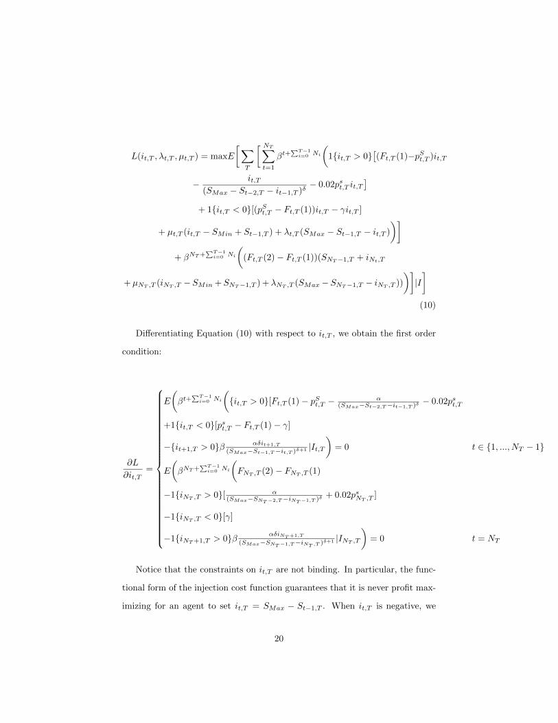
L(it,T , λt,T , µt,T ) = maxE

[∑T

[ NT∑t=1

βt+∑T−1i=0 Ni

(1{it,T > 0}

[(Ft,T (1)−pSt,T )it,T

− it,T(SMax − St−2,T − it−1,T )δ

− 0.02pst,T it,T]

+ 1{it,T < 0}[(pSt,T − Ft,T (1))it,T − γit,T ]

+ µt,T (it,T − SMin + St−1,T ) + λt,T (SMax − St−1,T − it,T )

)]+ βNT+

∑T−1i=0 Ni

((Ft,T (2)− Ft,T (1))(SNT−1,T + iNt,T

+µNT ,T (iNT ,T −SMin +SNT−1,T ) + λNT ,T (SMax−SNT−1,T − iNT ,T ))

)]|I](10)

Differentiating Equation (10) with respect to it,T , we obtain the first order

condition:

∂L

∂it,T=

E

(βt+

∑T−1i=0 Ni

({it,T > 0}[Ft,T (1)− pSt,T − α

(SMax−St−2,T−it−1,T )δ− 0.02pst,T

+1{it,T < 0}[pst,T − Ft,T (1)− γ]

−{it+1,T > 0}β αδit+1,T

(SMax−St−1,T−it,T )δ+1 |It,T)

= 0 t ∈ {1, ..., NT − 1}

E

(βNT+

∑T−1i=0 Ni

(FNT ,T (2)− FNT ,T (1)

−1{iNT ,T > 0}[ α(SMax−SNT−2,T−iNT−1,T )δ

+ 0.02psNT ,T ]

−1{iNT ,T < 0}[γ]

−1{iNT+1,T > 0}β αδiNT+1,T

(SMax−SNT−1,T−iNT ,T )δ+1 |INT ,T)

= 0 t = NT

Notice that the constraints on it,T are not binding. In particular, the func-

tional form of the injection cost function guarantees that it is never profit max-

imizing for an agent to set it,T = SMax − St−1,T . When it,T is negative, we

20

can assume an interior solution since inventory levels never approach the lower

bounds in the data set. Thus, both µt,T and λt,T from Equation (10) are set to

zero.

Essentially the first order condition stipulates that the expected marginal

value of injecting gas for time (t, T ) and (t + 1, T ) must equal the expected

marginal cost of doing so. Notice that the agent considers the effect of increasing

storage levels on injection costs when making injection decisions.

Without solving the entire system, we can estimate the injection cost param-

eter using the first order condition as a moment condition in a GMM setting.

Any vector that includes elements from the agent’s information set at time (t, T ),

such as past prices and storage levels, should be orthogonal to the first order

condition (7.3) since such a vector would contain no new information when the

agent makes its decision. These past observations can then provide instruments

to be used in a GMM framework. Define the matrix of instruments orthogonal

to the moment condition as zt, where zt is an m × q matrix, such that q ≥ 3

and m is the dimension of the sample size. We then have the following set of

moment equations,M :

M =

E

(z′(βt+

∑T−1i=0 Ni

({it,T > 0}[Ft,T (1)− pSt,T − α

(SMax−St−2,T−it−1,T )δ− 0.02pst,T

+1{it,T < 0}[pst,T − Ft,T (1)− γ]

−{it+1,T > 0}β αδit+1,T

(SMax−St−1,T−it,T )δ+1 )|It,T)

= 0 t ∈ {1, ..., NT − 1}

E

(z′(βNT+

∑T−1i=0 Ni

(FNT ,T (2)− FNT ,T (1)

−1{iNT ,T > 0}[ α(SMax−SNT−2,T−iNT−1,T )δ

+ 0.02psNT ,T ]

−1{iNT ,T < 0}[γ]

−1{iNT+1,T > 0}β αδiNT+1,T

(SMax−SNT−1,T−iNT ,T )δ+1 )|INT ,T)

= 0 t = NT

21

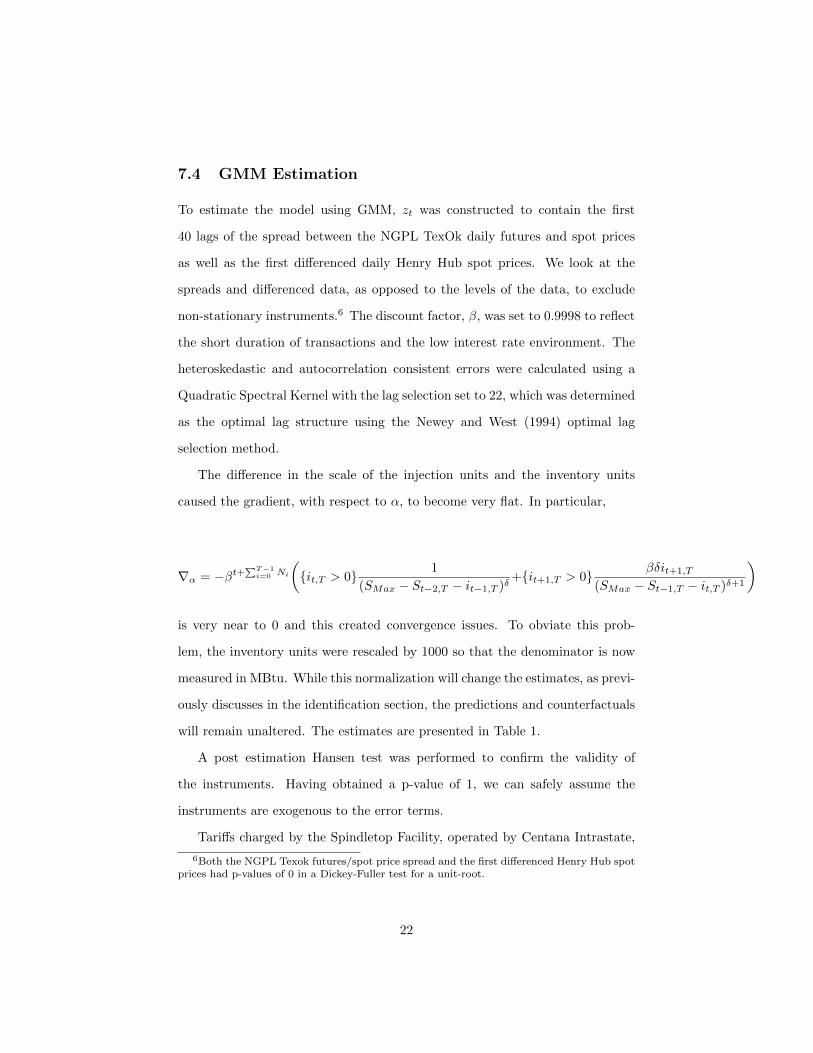
7.4 GMM Estimation

To estimate the model using GMM, zt was constructed to contain the first

40 lags of the spread between the NGPL TexOk daily futures and spot prices

as well as the first differenced daily Henry Hub spot prices. We look at the

spreads and differenced data, as opposed to the levels of the data, to exclude

non-stationary instruments.6 The discount factor, β, was set to 0.9998 to reflect

the short duration of transactions and the low interest rate environment. The

heteroskedastic and autocorrelation consistent errors were calculated using a

Quadratic Spectral Kernel with the lag selection set to 22, which was determined

as the optimal lag structure using the Newey and West (1994) optimal lag

selection method.

The difference in the scale of the injection units and the inventory units

caused the gradient, with respect to α, to become very flat. In particular,

∇α = −βt+∑T−1i=0 Ni

({it,T > 0} 1

(SMax − St−2,T − it−1,T )δ+{it+1,T > 0} βδit+1,T

(SMax − St−1,T − it,T )δ+1

)

is very near to 0 and this created convergence issues. To obviate this prob-

lem, the inventory units were rescaled by 1000 so that the denominator is now

measured in MBtu. While this normalization will change the estimates, as previ-

ously discusses in the identification section, the predictions and counterfactuals

will remain unaltered. The estimates are presented in Table 1.

A post estimation Hansen test was performed to confirm the validity of

the instruments. Having obtained a p-value of 1, we can safely assume the

instruments are exogenous to the error terms.

Tariffs charged by the Spindletop Facility, operated by Centana Intrastate,

6Both the NGPL Texok futures/spot price spread and the first differenced Henry Hub spotprices had p-values of 0 in a Dickey-Fuller test for a unit-root.

22

Table 1: Results

Cost Parameters

α .4178537 ∗∗∗∗

(35.76)

δ .4702111 ∗∗∗∗

(119.27)

γ .0331166∗∗∗∗

(399.82)

N 560

t statistics in parentheses∗ p < 0.1 ** p < 0.05, ∗∗∗ p < 0.01, ∗∗∗∗ p < 0.001

are posted by the Texas Railroad Commission, its state regulator. These rates

are subject to maximum injection and withdrawal rates. The estimated injection

cost function should provide some insight into rates that would be charged if

storage levels increased. In terms of the validity of the model, it accurately

predicts current prices given observed storage levels. The most recently posted

injection tariffs for the Spindletop Storage Facility are 0.01$/Mmbtu. The model

predicts the cost to inject one Mmbtu of gas, at the median level of storage

observed in the dataset, to be 0.009$ with a boostrapped standard error of

0.0028. Of course, we only have one observation point for comparison, but the

predictions for current costs are quite accurate given the information we have.

We can then more confidently examine some implications of these estimates in

the next section.

8 Examining the Impact of Increased Utiliza-

tion

We now explore how prices would change for different utilization rates of storage

in salt caverns. The base case cost, in other words the cost that is currently

23

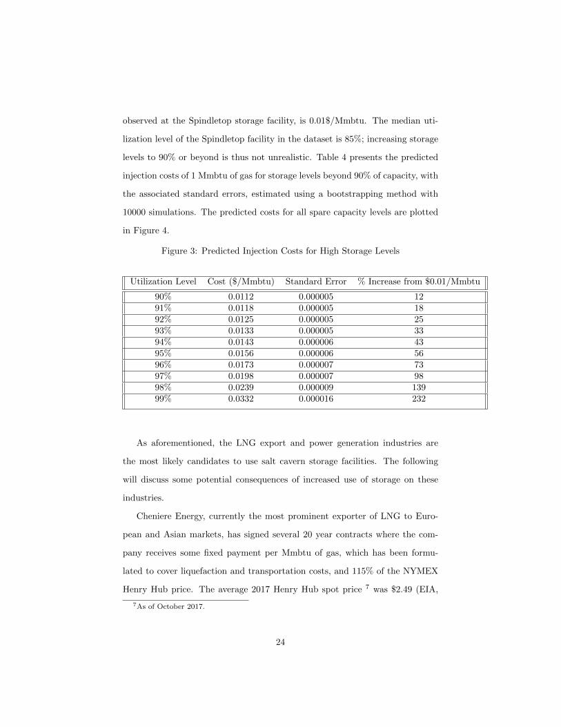
observed at the Spindletop storage facility, is 0.01$/Mmbtu. The median uti-

lization level of the Spindletop facility in the dataset is 85%; increasing storage

levels to 90% or beyond is thus not unrealistic. Table 4 presents the predicted

injection costs of 1 Mmbtu of gas for storage levels beyond 90% of capacity, with

the associated standard errors, estimated using a bootstrapping method with

10000 simulations. The predicted costs for all spare capacity levels are plotted

in Figure 4.

Figure 3: Predicted Injection Costs for High Storage Levels

Utilization Level Cost ($/Mmbtu) Standard Error % Increase from $0.01/Mmbtu

90% 0.0112 0.000005 1291% 0.0118 0.000005 1892% 0.0125 0.000005 2593% 0.0133 0.000005 3394% 0.0143 0.000006 4395% 0.0156 0.000006 5696% 0.0173 0.000007 7397% 0.0198 0.000007 9898% 0.0239 0.000009 13999% 0.0332 0.000016 232

As aforementioned, the LNG export and power generation industries are

the most likely candidates to use salt cavern storage facilities. The following

will discuss some potential consequences of increased use of storage on these

industries.

Cheniere Energy, currently the most prominent exporter of LNG to Euro-

pean and Asian markets, has signed several 20 year contracts where the com-

pany receives some fixed payment per Mmbtu of gas, which has been formu-

lated to cover liquefaction and transportation costs, and 115% of the NYMEX

Henry Hub price. The average 2017 Henry Hub spot price 7 was $2.49 (EIA,

7As of October 2017.

24

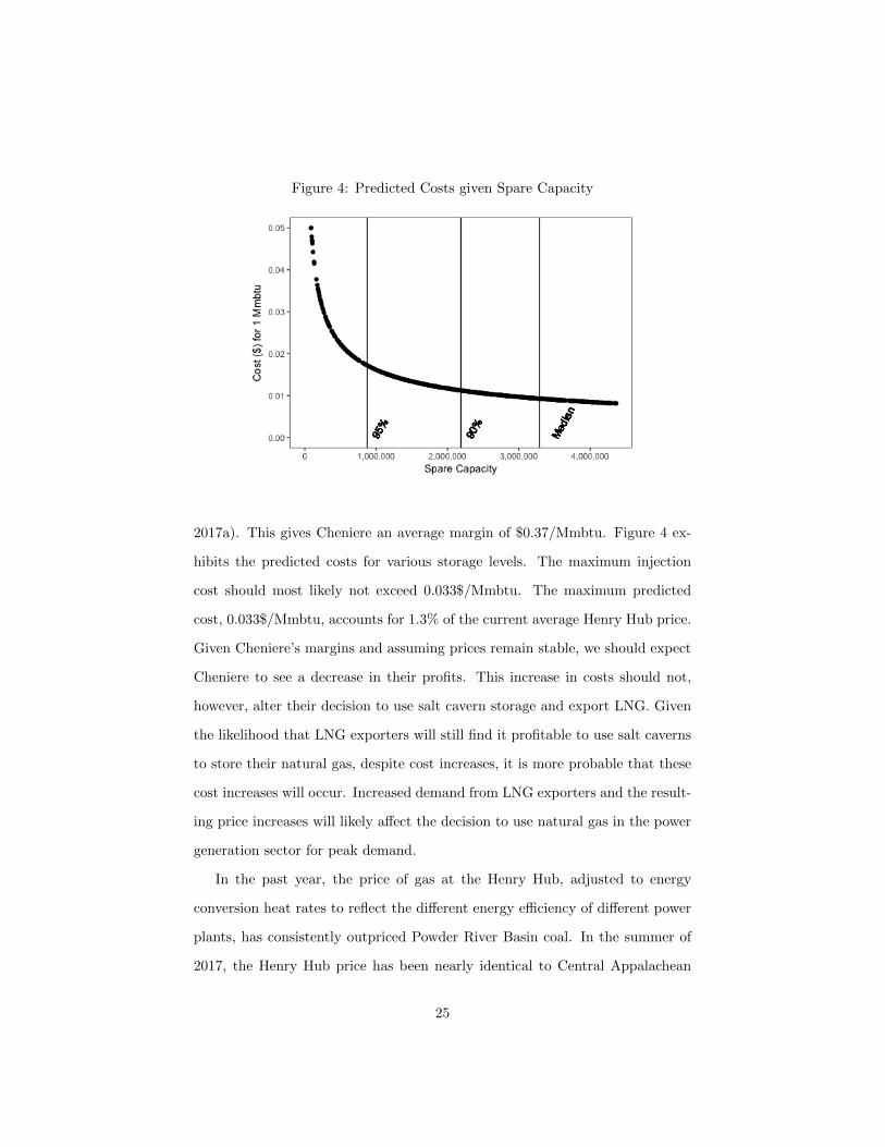
Figure 4: Predicted Costs given Spare Capacity

2017a). This gives Cheniere an average margin of $0.37/Mmbtu. Figure 4 ex-

hibits the predicted costs for various storage levels. The maximum injection

cost should most likely not exceed 0.033$/Mmbtu. The maximum predicted

cost, 0.033$/Mmbtu, accounts for 1.3% of the current average Henry Hub price.

Given Cheniere’s margins and assuming prices remain stable, we should expect

Cheniere to see a decrease in their profits. This increase in costs should not,

however, alter their decision to use salt cavern storage and export LNG. Given

the likelihood that LNG exporters will still find it profitable to use salt caverns

to store their natural gas, despite cost increases, it is more probable that these

cost increases will occur. Increased demand from LNG exporters and the result-

ing price increases will likely affect the decision to use natural gas in the power

generation sector for peak demand.

In the past year, the price of gas at the Henry Hub, adjusted to energy

conversion heat rates to reflect the different energy efficiency of different power

plants, has consistently outpriced Powder River Basin coal. In the summer of

2017, the Henry Hub price has been nearly identical to Central Appalachean

25

coal EIA (2017). Increased utilization of salt caverns in the Gulf region, which

as described above is likely, would put additional upward pressure on the cost

to generate power with natural gas. Given spare capacity rates of 90%-99%,

storage injection costs could be anywhere from 0.45% to 1.3% of the current

average yearly Henry Hub price. While these costs may not seem significant,

they can cause natural gas to lose favor to coal on the margin. Of course, demand

for coal and gas in power generation is a multifaceted problem and depends on

more than just spot prices, but higher gas prices, spurred by increased injection

costs into storage and heightened demand for gas exports, would certainly not

encourage demand for gas.

9 Conclusions and Policy Implications

There will most likely be a greater use of salt cavern storage in the Gulf region

in future years. Increased LNG exports from the area, as well as the electric

sector’s growing reliance on natural gas, will put increasing pressure on the

existing underground storage capacity.

Since injection and withdrawal costs are sensitive to the amount of pressure

in the storage facility, they are likely to change in the coming years with in-

creased use of the facilities. This paper has provided estimates on how injection

costs will change as storage is used more extensively, using a GMM estima-

tion technique that recovers the unknown parameters from profit maximization

assumptions and observed injection/withdrawal rates. The estimated results

imply that as storage levels approach capacity, injection costs increase at an

increasing rate.

The quantification of an injection cost function into salt cavern storage is

an important finding for determining natural gas pricing and understanding the

behavior of short term natural gas traders, who have a considerable influence

26

on the market. At the theoretical level, it should also aid in building models

that seek to determine the value of natural gas storage facilities. The landscape

of the U.S. natural gas market has greatly changed in the past few years and

continues to do so, mainly in response to the Shale Revolution and the beginning

of U.S. LNG exports. The natural gas storage industry is due to change with

it.

27

References

American Gas Association (2017). FERC Order 636 637.

https://www.aga.org/federal-regulatory-issues-and-advocacy/ferc-order-

636-637 [Dataset][Accessed July 2017].

Boogert, A. and C. De Jong (2008). Gas storage valuation using a monte carlo

method. The journal of derivatives 15 (3), 81–98.

Chen, Z. and P. A. Forsyth (2007). A semi-lagrangian approach for natural

gas storage valuation and optimal operation. SIAM Journal on Scientific

Computing 30 (1), 339–368.

Cooper, R., J. C. Haltiwanger, and J. L. Willis (2010). Euler-equation estima-

tion for discrete choice models: A capital accumulation application. Technical

report, National Bureau of Economic Research.

Cortes, M. F. (2010). Gas storage valuation. University of Amsterdam Thesis.

DEA (2017). Technology. http://www.dea-speicher.de/en/technology

[Dataset][Accessed July 2017].

EIA (2015a). Natural gas salt-facility storage serves special gas market needs .

https://www.eia.gov/todayinenergy/detail.php?id=22232 [Dataset][Accessed

August 2017].

EIA (2015b). The Basics of Underground Natural Gas Storage.

https://www.eia.gov/naturalgas/storage/basics/ [Dataset][Accessed July

2017].

EIA (2017a). Natural Gas. https://www.eia.gov/dnav/ng/hist/rngwhhdA.htm

[Dataset][Accessed October 2017].

28

EIA (2017b). Underground Natural Gas Working Storage Capacity.

https://www.eia.gov/naturalgas/storagecapacity/ [Dataset][Accessed July

2017].

EIA (2017c). United States expected to become a net exporter of natu-

ral gas this year. https://www.eia.gov/todayinenergy/detail.php?id=32412

[Dataset][Accessed August 2017].

EIA (2017d). What are Ccf, Mcf, Btu, and therms? How do I convert nat-

ural gas prices in dollars per Ccf or Mcf to dollars per Btu or therm?

https://www.eia.gov/tools/faqs/faq.php?id=45t=8 [Dataset][Accessed July

2017].

EIA (2017). What is U.S. electricity generation by source?

https://www.eia.gov/tools/faqs/faq.php?id=427t=3 [Dataset][Accessed

July 2017].

Fairway Energy (2017). Underground Storage Overview.

http://www.fairwaymidstream.com/capabilities/underground-storage-

overview.html [Dataset][Accessed July 2017].

Fang, H., A. Ciatto, and F. Brock (2016). U.S. Natural Gas Storage Capacity

and Utilization Outlook. https://energy.gov/epsa/downloads/us-natural-gas-

storage-capacity-and-utilization-outlook [Dataset][Accessed July 2017].

FERC (2004). Current State of and Issues Concerning Underground Natural

Gas Storage. https://www.ferc.gov/EventCalendar/Files/20041020081349-

final-gs-report.pdf [Dataset][Accessed August 2017].

Hansen, L. P. and K. J. Singleton (1982). Generalized instrumental variables

estimation of nonlinear rational expectations models. Econometrica: Journal

of the Econometric Society , 1269–1286.

29

Henaff, P., I. Laachir, and F. Russo (2013). Gas storage valuation and hedging.

a quantification of the model risk. arXiv preprint arXiv:1312.3789 .

Li, Y. (2007). Natural gas storage valuation. Georgia Institute of Technology

Thesis.

Natural Gas Supply Association (2014). Storage of Natural Gas.

http://naturalgas.org/naturalgas/storage/ [Dataset][Accessed July 2017].

Newey, W. K. and K. D. West (1994). Automatic lag selection in covariance

matrix estimation. The Review of Economic Studies 61 (4), 631–653.

Schoppe, J. (2010). The valuation of natural gas storage: a knowledge gradi-

ent approach with non-parametric estimation. Bachelor Thesis of Science in

Engineering, Department of Operations Research and Financial Engineering,

Princeton University .

Thompson, M., M. Davison, and H. Rasmussen (2009). Natural gas storage val-

uation and optimization: A real options application. Naval Research Logistics

(NRL) 56 (3), 226–238.

30