Cop

yrig

ht 2

006

SIEP

B.V

.

Sh

ell E

xplo

ratio

n &

Pro

duct

ion

EPT

Shell Exploration & Production

Estimating extreme wave design criteria incorporating directionality

Kevin EwansShell International Exploration and Production

Philip JonathanShell Research Limited

Cop

yrig

ht 2

005

SIE

P B.

V.

Shel

l Exp

lora

tion

& P

rodu

ctio

n

E

PS-H

SE

P

0462

7_00

2 Sl

.2

Overview• Motivation

• Data

• Directional extremal model

• Estimating omni-directional extremes

• Design criteria for directional extremes

• Conclusions

Cop

yrig

ht 2

005

SIE

P B.

V.

Shel

l Exp

lora

tion

& P

rodu

ctio

n

E

PS-H

SE

P

0462

7_00

2 Sl

.3

Motivation• In most regions, but particularly hurricane-dominated regions (e.g. Gulf of Mexico), and in regions where extra-tropical storms prevail (e.g. Northern North Sea), the extremal properties of storms are also highly dependent on storm direction

• Sea state design criteria for offshore facilities are frequently provided by direction to optimise engineering factilities

• Important that these criteria be consistent so that the probability ofexceedance of a given wave height from any direction derived from the directional values is the same as for the omni-directional value.

• No consensus on how the criteria should be specified

Cop

yrig

ht 2

005

SIE

P B.

V.

Shel

l Exp

lora

tion

& P

rodu

ctio

n

E

PS-H

SE

P

0462

7_00

2 Sl

.4

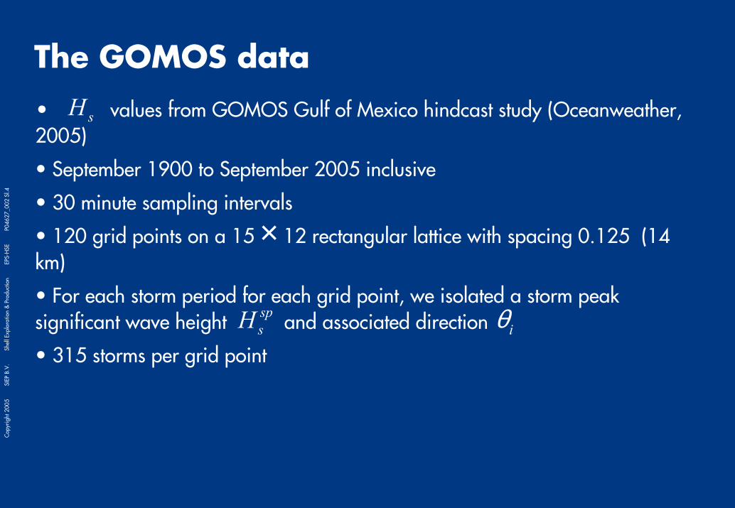
The GOMOS data• values from GOMOS Gulf of Mexico hindcast study (Oceanweather, 2005)

• September 1900 to September 2005 inclusive

• 30 minute sampling intervals

• 120 grid points on a 15 12 rectangular lattice with spacing 0.125 (14 km)

• For each storm period for each grid point, we isolated a storm peak significant wave height and associated direction

• 315 storms per grid point

sH

×

spsH iθ

Cop

yrig

ht 2

005

SIE

P B.

V.

Shel

l Exp

lora

tion

& P

rodu

ctio

n

E

PS-H

SE

P

0462

7_00

2 Sl

.5

The GOMOS data

Cop

yrig

ht 2

005

SIE

P B.

V.

Shel

l Exp

lora

tion

& P

rodu

ctio

n

E

PS-H

SE

P

0462

7_00

2 Sl

.6

The GOMOS data

These locations are 250 km apart

Cop

yrig

ht 2

005

SIE

P B.

V.

Shel

l Exp

lora

tion

& P

rodu

ctio

n

E

PS-H

SE

P

0462

7_00

2 Sl

.7

The directional extremal model

( ) ( ) ( )( )

( )( )γ θ

θγ θ

θσ θ

−

+

= ≤ = − + −

1

| , | , 1 1 iX u i i

i

iF x P X x u x ui iCDF:

( )iγ θ ( )iσ θ uscale parametershape parameter or tail index

threshold (assumed constant with direction)

Parameters characterised by Fourier series expansion (e.g. Robinson & Tawn, 1997)

( ) ( )( ) ( )( )

( ) ( )( ) ( )( )

11 120

21 220

cos sin

cos sin

p

k kkp

k kk

A k A k

A k A k

γ θ θ θ

σ θ θ θ

=

=

= +

= +

∑

∑

Parameters estimated by maximum likelihood

Cop

yrig

ht 2

005

SIE

P B.

V.

Shel

l Exp

lora

tion

& P

rodu

ctio

n

E

PS-H

SE

P

0462

7_00

2 Sl

.8

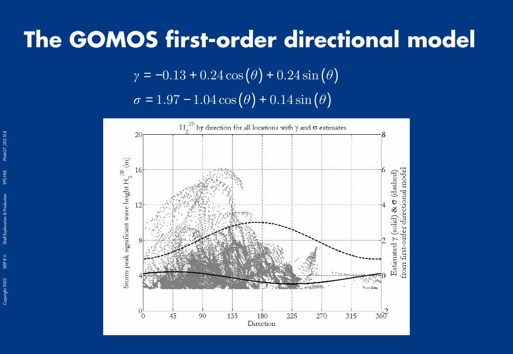
The GOMOS first-order directional model( ) ( )

( ) ( )γ θ θ

σ θ θ

= − + +

= − +

0.13 0.24 cos 0.24 sin

1.97 1.04 cos 0.14 sin

Cop

yrig

ht 2

005

SIE

P B.

V.

Shel

l Exp

lora

tion

& P

rodu

ctio

n

E

PS-H

SE

P

0462

7_00

2 Sl

.9

Comparison of higher order models

Cop

yrig

ht 2

005

SIE

P B.

V.

Shel

l Exp

lora

tion

& P

rodu

ctio

n

E

PS-H

SE

P

0462

7_00

2 Sl

.10

First-order model confidence bands

Cop

yrig

ht 2

005

SIE

P B.

V.

Shel

l Exp

lora

tion

& P

rodu

ctio

n

E

PS-H

SE

P

0462

7_00

2 Sl

.11

Estimation of omni-direction ExtremesAssume

• Given storm peak direction, , storm peak above follows GPD with parameters and

• Storm occurrences are independent Poisson events with expectation per annum per storm

• Storm peak directions for any period are restricted to

sH

0

1P

{ } 1

ni i

θ=

iθ

P

u( )iγ θ ( )iσ θ

Cop

yrig

ht 2

005

SIE

P B.

V.

Shel

l Exp

lora

tion

& P

rodu

ctio

n

E

PS-H

SE

P

0462

7_00

2 Sl

.12

Estimation of omni-direction extremes

Cop

yrig

ht 2

005

SIE

P B.

V.

Shel

l Exp

lora

tion

& P

rodu

ctio

n

E

PS-H

SE

P

0462

7_00

2 Sl

.13

Estimation of omni-direction extremesDistribution of the maximum storm within a given sector in a given period is given by:

sHP

S

( ) ( )

( )( ) ( )

( )( ) ( )

( )

max max

01

1

1

| , [1, 2,..., ]

| ,

exp 1i

X S S i

n

i i i i iki

ni

i i i

F x P X x X u i i n

P S X x X u M k P M k

xm uS

γ θ

ρ

γ θσ θ ρ

∞

==

−

=

= ≤ > ∀ ∈

= ≤ > = =

= − + −

∑∏

∑

is the expected value of the number of occurrences of storm which is assumed to follow a Poisson distribution

0

PmP

=where

Cop

yrig

ht 2

005

SIE

P B.

V.

Shel

l Exp

lora

tion

& P

rodu

ctio

n

E

PS-H

SE

P

0462

7_00

2 Sl

.14

GOMOS quadrant & omni extremes

Cop

yrig

ht 2

005

SIE

P B.

V.

Shel

l Exp

lora

tion

& P

rodu

ctio

n

E

PS-H

SE

P

0462

7_00

2 Sl

.15

Design criteria for directional extremes

Omni-directional 100-yr maximum cumulative probability

( ) ( )max100 max1001

m

Omni Si

P X x P X xi=

≤ = ≤∏where P X( )max100S xj ≤ is cumulative probability for the maximum in

the sectors in a 100-yr period{ } 1mi iS =

The 100-yr design can be calculated for a particular non-exceedance probability from

sH100Omniq

( )100 max100 100Omni Omni Omniq P X x= ≤

Specification of does not allow unique values of the sector 100-yr design

100Omniq

sH

Cop

yrig

ht 2

005

SIE

P B.

V.

Shel

l Exp

lora

tion

& P

rodu

ctio

n

E

PS-H

SE

P

0462

7_00

2 Sl

.16

Design criteria for directional extremesCASE I: All but one sectors have negative shape parameter

Each sector with negative shape parameter has an upper limit of storm peak sH

Set design values for each of these sectors to the maximum, with =100 1Sq i

and 100 100 1001

m

Omni S Siq q qi=

= ∏ = ∗

where *S is the remaining sector with positive shape parameter

Cop

yrig

ht 2

005

SIE

P B.

V.

Shel

l Exp

lora

tion

& P

rodu

ctio

n

E

PS-H

SE

P

0462

7_00

2 Sl

.17

Design criteria for directional extremesCASE II: All sectors set to omni-direction 100s OmniH

( )100 max100 100S S Omniq P X xi i= ≤ i∀set

• non-exceedance probabilities different for

• non-exceedance probability for most severe sector less than less severe

• non-exceedance probability for most severe at least as large as omni-direction

each sector

Cop

yrig

ht 2

005

SIE

P B.

V.

Shel

l Exp

lora

tion

& P

rodu

ctio

n

E

PS-H

SE

P

0462

7_00

2 Sl

.18

Design criteria for directional extremesCASE III: All sectors have equal non-exceedance probability

set

• sets 100m return-period levels for each sector

• most severe sector higher the the an than omni-direction value

• setting the most extreme sector to 100m-year level might be “over-conservative”

( )100 100 1001

m mOmni S S

iq q q

== ∏ = where ( )100 100

1S Omni mq q=

100 is SH

Cop

yrig

ht 2

005

SIE

P B.

V.

Shel

l Exp

lora

tion

& P

rodu

ctio

n

E

PS-H

SE

P

0462

7_00

2 Sl

.19

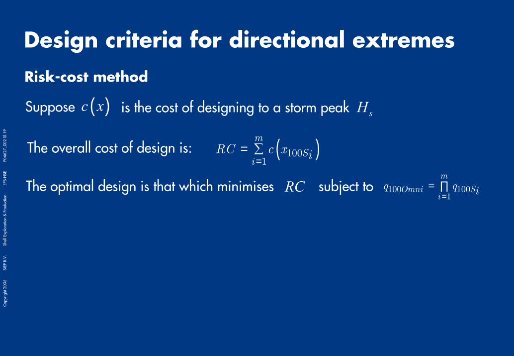
Design criteria for directional extremesRisk-cost method

Suppose is the cost of designing to a storm peak ( )c x sH

( )1001

m

Si

RC c x i== ∑The overall cost of design is:

The optimal design is that which minimises subject to RC 100 1001

m

Omni Si

q q i== ∏

Cop

yrig

ht 2

005

SIE

P B.

V.

Shel

l Exp

lora

tion

& P

rodu

ctio

n

E

PS-H

SE

P

0462

7_00

2 Sl

.20

Design criteria for directional extremesRisk-cost method – two sector example ( ) = 20.001c x x

• total design cost for

• optimal design cost balance between “omni-directional design” and “equal non-exceedances design”

=100 0.5Omniq

Cop

yrig

ht 2

005

SIE

P B.

V.

Shel

l Exp

lora

tion

& P

rodu

ctio

n

E

PS-H

SE

P

0462

7_00

2 Sl

.21

Design criteria for directional extremes

Sector RC RC RC

[0,90) 8.78 18.03 0.75 9.73 15.60 0.59 9.29 20.20 0.84

[90,180) 8.78 17.40 0.81 9.73 15.60 0.69 9.29 17.90 0.84

[180,270) 8.78 11.44 0.91 9.73 15.60 0.98 9.29 10.30 0.84

[270,360) 8.78 10.90 0.90 9.73 15.60 0.98 9.29 9.70 0.84

[0,90) 7.56 15.00 0.82 7.84 14.00 0.72 7.59 15.20 0.84

[90,180) 7.56 15.40 0.82 7.84 14.00 0.66 7.59 15.70 0.84

[180,270) 7.56 13.41 0.84 7.84 14.00 0.88 7.59 13.40 0.84

[270,360) 7.56 10.67 0.89 7.84 14.00 0.98 7.59 10.10 0.84

Equal sector non-exceedance

Dire

ctio

nal

Mod

el

Dire

ctio

n-in

depe

nden

t m

odel

Risk-cost optimal Omni-direction

Design criteria based on median omni-directional 100s OmniH

100 iSx 100 iS

x100 iSx100 iS

q 100 iSq 100 iS

q

• Directional model design values > Direction independent values

• RC model avoids large range of and of other two methods

• RC model design based on directional EV model is preferable

100 iSq 100 iS

x

Cop

yrig

ht 2

005

SIE

P B.

V.

Shel

l Exp

lora

tion

& P

rodu

ctio

n

E

PS-H

SE

P

0462

7_00

2 Sl

.22

Conclusions• Strong general case for adopting directional extreme model to storm peak [unless it can be demonstrated statistically that a direction free model is no less appropriate].

• A directional extremes model [e.g. Fourier series expansion] allows directionally consistent extreme values to be derived.

• Important to consider directionality of sea states when developing design criteria [omni-directional extremes from directional data can be significantly different from a direction-independent derivation].

– Even when the extremal characteristics of storm peak are direction independent rate of occurrence of storms is dependent on storm direction – the distribution of will have directional dependence in general.

• Risk-cost method is an objective approach to optimise directional criteria, while preserving overall reliability [RC method avoids more extreme properties of other design methods].

100sH

sH

sH