estimating covariation: epps effect, microstructure noise · estimate covariation with high...

Estimating Covariation: Epps Effect, Microstructure Noise ∗

Lan ZhangDepartment of Finance

University of Illinois at ChicagoChicago, IL 60607

E-mail: [email protected]

Original version: June 21, 2005Previous version: October 24, 2008

This version: July 2, 2009

Abstract

This paper is about how to estimate the integrated covariance 〈X,Y 〉T of two assets over a fixed timehorizon [0, T ], when the observations of X and Y are “contaminated” and when such noisy observationsare at discrete, but not synchronized, times. We show that the usual previous-tick covariance estimatoris biased, and the size of the bias is more pronounced for less liquid assets. This is an analytic charac-terization of the Epps effect. We also provide optimal sampling frequency which balances the tradeoffbetween the bias and various sources of stochastic error terms, including nonsynchronous trading, mi-crostructure noise, and time discretization. Finally, a two-scales covariance estimator is provided whichsimultaneously cancels (to first order) the Epps effect and the effect of microstructure noise. The gain isdemonstrated in data.

KEYWORDS: Bias-variance tradeoff; Epps effect; High frequency data; Measurement error; Mar-ket Microstructure; Martingale; Nonsynchronous trading; Realized covariance; Realized variance; Twoscales estimation.

JEL CODES: C01; C13; C14; C46; G11

∗The author would like to thank the editors and referees for helpful and constructive comments.

Estimate covariation with high frequency noisy data 2

1. Introduction

This paper is about how to estimate the integrated covariance 〈X,Y 〉T over a fixed time horizon [0, T ], whenthe observations of X and Y are “contaminated” and when such noisy observations of X and of Y are atdiscrete, but not synchronized, times.

Consider the price processes of two assets, {Xt} and {Yt}, both in logarithmic scale. Suppose both{Xt} and {Yt} follow an Ito process, namely,

dXt = µXt dt+ σXt dBXt , (1)

dYt = µYt dt+ σYt dBYt , (2)

where BX and BY are standard Brownian motions, with correlation corr(BXt , B

Yt ) = ρt. The drift coeffi-

cient µt, and the instantaneous variance σ2t of the returns process Xt will be stochastic processes, which are

assumed to be locally bounded.

Our interest is to estimate the integrated covariation 〈X,Y 〉T ,

〈X,Y 〉T =∫ T

0σXt σ

Yt d〈BX , BY 〉t, (3)

using the ultra-high frequency observations of X and Y within the fixed time horizon [0, T ]. Inference for(3) is a well-understood problem if X and Y are observed simultaneously and without contamination (say,in the form of microstructure noise). A limit theorem in stochastic processes states that

∑i:τi∈[0,T ](Xτi −

Xτi−1)(Yτi − Yτi−1), commonly called realized covariance, is a consistent estimator for 〈X,Y 〉T as theobservation intervals get closer; furthermore its estimation error follows a mixed normal distribution, see, forexample, Jacod and Protter (1998), Barndorff-Nielsen and Shephard (2002a), Zhang (2001), and Myklandand Zhang (2006). For a glimpse of the econometric literature on this inference problem when X = Y ,one can read Andersen and Bollerslev (1998), Andersen, Bollerslev, Diebold, and Labys (2001), Barndorff-Nielsen and Shephard (2002b), and Gencay, Ballocchi, Dacorogna, Olsen, and Pictet (2002), among others.

In ultra-high frequency data, the exact observation times of X and Y are rarely simultaneous, andestimating 〈X,Y 〉T in this asynchronous case becomes a relevant and pressing problem. This lack of syn-chronicity often causes some undesirable features in the inference. In particular, as documented by Epps(1979), correlation estimates tend to decrease when sampling is done at high frequencies. Even in daily data,asynchronicity can cause difficulties (Scholes and Williams (1977)). Lo and MacKinlay (1990) propose asolution based on a stochastic model of censoring. In practice, most nonparametric estimation proceduresfor 〈X,Y 〉T start with creating an approximately synchronized pair (X,Y ) by either previous-tick inter-polation or linear interpolation, then construct the estimator on the basis of the synchronized approxima-tions. These interpolation-based estimators are often biased, as witnessed in empirical studies (Dacorogna,Gencay, Muller, Olsen, and Pictet (2001)).

A different issue when one deals with high frequency data is the existence of microstructure noise.In the early papers (Aıt-Sahalia, Mykland, and Zhang (2005), Zhang, Mykland, and Aıt-Sahalia (2005)),they found that when the microstructure noise is present in the observed prices, then the realized varianceestimator for 〈X,X〉T – a special case of realized covariance – is biased and this bias can get progressivelyworse as more high frequency data is employed.1 However, it is not well understood how an estimator forthe covariation 〈X,Y 〉T behaves, when the estimation uses ultra-high frequency noisy data.

1Recent developments on volatility estimation include multi-scale estimation (Zhang (2006), Aıt-Sahalia, Mykland, and Zhang


In this paper, we are concerned with the behavior of the previous-tick approach to estimation of 〈X,Y 〉Twhen the observation times ofX and Y are not synchronized and when the microstructure noise is present inthe observed price processes. We show that asynchronicity leads to a bias in the previous-tick estimator for〈X,Y 〉T , thus giving an analytic form of the Epps effect. The variance of the estimator, meanwhile, comesfrom three sources – discrete observation/transaction times, nonsynchronization, and the microstructurenoise. We provide the optimal sampling frequency to balance the tradeoff among different error sources,and present the explicit expression for the asymptotic bias and variance when the observations times of Xand Y follow Poisson process.

A further advantage of the previous tick estimator is that it permits easy analysis of microstructure noise.It is here shown that in the presence of noise, one can create two and multi scale versions of the previoustick estimator. As we shall see in Section 8, the bias due to asynchronicity cancels in the same way as thebias due to microstructure noise, while the variance asymptotically behaves as if there is no asynchronicity(in the subsample of previous ticks). Thus, while the previous tick approach does throw away data, it canretain rate efficiency.

In terms of microstructure noise, this paper provides a two- and multiscale alternative to the multivariateautocovariance-based estimator of Barndorff-Nielsen, Hansen, Lunde, and Shephard (2008b). Other workinvestigating the combination of asynchronicity and microstructure noise includes Lunde and Voev (2007)and Griffin and Oomen (2007).

The paper is organized as follows: we introduce the concepts and notations in Section 2.1, and give apreview of the main findings in Section 2.2. Section 3 and 4 provide the asymptotic stochastic bias andvariance of the previous-tick estimator, assuming the absence of microstructure noise in the price processes.Section 5 deals with the case when the trading times are random. An application when the transaction timesfollow Poisson processes is provided in Section 6. Section 7 focuses on the inference when the microstruc-ture noise is present. Two scales estimation is presented in Section 8. Finally, Section 9 concludes.

2. Setting, and some Main Findings

2.1. Setup and Notations

Our interest is to estimate the covariation 〈X,Y 〉T between two returns in a fixed time period [0, T ], whenX and Y are observed asynchronously.

Let the observation/transaction times of X be recorded in Tn, and those of Y in Sm. At the momentwe assume X and Y are free of microstructure noise (in short, noise). Later in Section 7 we study thecases when these two price processes are observed with noise εX and εY respectively. We denote theelements in Tn by τn,i, and the elements in Sm by θm,i. Specifically, 0 = τn,0 ≤ τn,1 ≤ . . . ≤ τn,n = T ,0 = θm,0 ≤ θm,1 ≤ . . . ≤ θm,m = T . For the ease of the notation, we often suppress the subscript n andm from the τs and θs unless the context is misleading. The τ and θ sequences may be irregular and randombut independent of the price process, so long as the spacings are not allowed to be too large. An extensionto more general random times is considered in Section 5.

We focus on a particular type of covariance estimator called previous-tick estimator. Intuitively, it is

(2009)), kernel methods (Barndorff-Nielsen, Hansen, Lunde, and Shephard (2008a, 2009)), and pre-averaging (Podolskij and Vetter(2009) , Jacod, Li, Mykland, Podolskij, and Vetter (2009)).


a sample covariance estimator based on the prices that immediately precede (or are at) the pre-specifiedsampling points. One can view this previous-tick approach as a special way to subsample the raw data.

To formulate the previous-tick covariance estimator, we introduce the concepts related to samplingpoints. Let

N = n+m,

write n and m as nN and mN from here on.

We consider a subset of [0, T ] which satisfies the following.

VN ⊂ [0, T ]; 0, T ∈ VN , also VN is finite for each N. (4)

We use vi to denote the elements in VN , VN = {v0, v1, . . . , vMN}, with v0 = 0 and vMN

= T , whereMN is the sampling frequency. A simple case of V would be a regular grid, where the elements are equallyspaced out in time, that is, vi− vi−1 = ∆v,∀i. This sampling scheme is the most common one in analyzingtime-dependent data, for example, typical sampling interval in high-frequency financial application includesevery 5 minutes, 15 minutes, 30 minutes and hourly.

An alternative way of setting the grid VN is to let the vi’s depend on the observation times, for exampleby setting vi to be the maximum of min{τ ∈ Tn : τ > vi−1} and min{θ ∈ Sm : θ > vi−1}. This is theconcept of refresh time, as introduced by Barndorff-Nielsen, Hansen, Lunde, and Shephard (2008b). Onecan also implement this for more than two stocks.

We assume the following regarding the relation between vis, τis, and θis:

CONDITION C1: There is at least one pair of (τ, θ) in between the consecutive vis.

Under Condition C1, the previous ticks are then defined as:

ti = max{τ ∈ Tn : τ ≤ vi}, and si = max{θ ∈ Sm : θ ≤ vi}, (5)

so that the tis and the sis are the sampling points in X and Y , respectively, according to the previous-ticksampling scheme. We note that condition C1 holds so long as there are sufficiently many data in both Xand Y within the time window [0, T ]. A sufficient criterion for C1 is provided by Conditions C2-C3 below.C1 is also valid (without C3) when the v’s are the refresh times mentioned above.

We need more assumptions to pursue the analysis for the covariance estimator. We assume that thetransaction times of X and Y satisfy:

CONDITION C2: supi |θm,i − θm,i−1| = O( 1N ), and supi |τn,i − τn,i−1| = O( 1

N ).

Note that Condition C2 implies that on the one hand lim infN→∞ mNN > 0 and lim infN→∞ nN

N > 0;on the other hand, it is obvious that mNN ≤ 1 and nN

N ≤ 1. In particular, nN = O(mN ) and mN = O(nN ).We sometimes assume that the sampling frequency MN satisfies:

CONDITION C3: supi |vN,i − vN,i−1| = O( 1MN

), and MN = o(N).

Conditions C2-C3 imply Condition C1 when N is large enough.

There are two reasons for imposing C3. One is technical, it arises naturally in connection with bothtwo scales estimation (Section 8) and bias-variance tradeoffs (Sections 4.3, 6.2 and 7.1). The other is moreconceptual: the observation times are often not known exactly or incorrectly recorded. If one assumes thatthe times are known up to, say, order O(N−α), having the distance between consecutive grid points in V ,vi − vi−1, bigger than O(N−α) ensures the previous-tick estimator to be consistent.


Definition 1. At last, the previous-tick estimator for the covariation is defined as

[X,Y ]T =MN∑i=1

(Xti −Xti−1)(Ysi − Ysi−1), (6)

where the tis and sis are the previous ticks in (5).

2.2. Some Main Findings

We here summarize the most important results from the practitioner point of view. First of all, the bias inthe estimator (6) is given by

−∫ T

0〈X,Y 〉′udFN (u) +Op(

1N

), (7)

where FN (t) =∑

i:max(ti,si)≤t |ti − si|. Typically, FN (t) and the bias are of order Op(MN/N). SeeTheorem 1 for precise statements. Second, when Condition C3 is in place, then

[X,Y ]T = [X,Y ]T −∫ T

0〈X,Y 〉′udFN (u) +Op(N−1/2) (8)

where [X,Y ]T is the unobserved value of the synchronized estimator

[X,Y ]T =MN∑i=1

(Xvi −Xvi−1)(Yvi − Yvi−1). (9)

See Theorem 4 (in Section 4.1) for details. Under condition C3, therefore, one can behave as if observationswere synchronously obtained at times vi, provided that one can deal with the bias. This has importantconsequences. On the one hand, it provides an analytic characterization of the Epps (1979) effect. Asdescribed further in Section 3.2, the Epps effect is essentially the bias (7), and it is typically negative forpositively associated processes (X,Y ). Also, from (8), the Epps effect is only a matter of bias; except atthe highest sampling frequencies, it does not substantially affect the variance of the estimator. On the otherhand, (8) suggests that when suitably adapted, existing theory for the synchronized case can be applied tothe asynchronous case.

We shall show two types of applications. In Sections 4.3, 6.2, and 7.1, we carry out a bias-variance trade-off to remove the effect of asynchronicity. In Section 8 we show that both asynchronicity and microstructurenoise can be removed with the help of two-scales estimation, along the lines of Zhang, Mykland, and Aıt-Sahalia (2005).

3. Previous-tick covariance estimator under zero noise

We start with an idealized world, where the mechanics of the trading process is perfect so that there is nomicrostructure noise in both X and Y . We shall see that [X,Y ]T can be decomposed based on the impactof different data structure.


3.1. Decomposition for the estimator [X, Y ]T

Let X and Y be Ito processes satisfying (1)-(2). Let [X,Y ]T be the previous-tick covariance estimator in(6). From the Kunita-Watanabe inequality, 〈X,Y 〉t is absolutely continuous in t. Assuming Condition C1,we can therefore decompose [X,Y ]T into:

[X,Y ]T =∑i

∫ min(ti,si)

max(ti−1,si−1)〈X,Y 〉′udu︸︷︷︸

drift term

+∑i

∫ min(ti,si)

max(ti−1,si−1)(Xu −Xmax(ti−1,si−1))dYu[2]︸︷︷︸

LN , discretization error

+ RN︸︷︷︸asynchronicity error

, (10)

where the tis and sis are the previous ticks defined in (5), and see Lemma 1 in Appendix for the exact formof RN . We have used the following symbol (cf. McCullagh (1987)):

Notation 1. The symbol “[2]” is used as follows: if (a, b) is an expression in a and b, then (a, b)[2]means (a, b) + (b, a), so that (Xu − Xmax(ti−1,si−1))dYu[2] means (Xu − Xmax(ti−1,si−1))dYu + (Yu −Ymax(ti−1,si−1))dXu.

Each component in (10) plays different role in the distribution of [X,Y ]T . To proceed the discussion,we need first to define stochastic bias and stochastic variance of an estimator.

Definition 2. Consider a semimartingale Z. Let Z be an estimator for Z. Suppose that Zt − Zt has thefollowing Doob-Meyer decomposition, for t ∈ [0, T ],

Zt − Zt = At +Mt,

where {Mt} is a martingale and {At} is a predictable process. Then for fixed t, t ∈ [0, T ], we call At thestochastic bias of Zt, denoted as SBias(Zt); we call the quadratic variation 〈M,M〉t of Mt the stochasticvariance of Zt.

Note that if At is nonrandom, it is also the exact bias; if 〈M,M〉t is nonrandom, it gives the exactvariance.

In light of Definition 2 and the decomposition equation (10), the stochastic bias of [X,Y ]T is∑i

∫ min(ti,si)

max(ti−1,si−1)〈X,Y 〉′udu− 〈X,Y 〉T ;

meanwhile, both the discretization error LN and the asynchronicity error RN contribute to the stochasticvariance of [X,Y ]T . It is apparent that, in the situation when X and Y are traded simultaneously, theasynchronicity error RN becomes zero. When the trading is not synchronous, however, it is not obvious tosee the relative impact and the trade-off between LN and RN . We pursue these next. First, we need thefollowing concept.

Definition 3. A sequence of cadlag processes GN (t), 0 ≤ t ≤ T is said to be relatively compact in prob-ability (RCP) if every subsequence has a further subsequence GNk so that there is a process G(t), whereGNk(t) converges in probability to G(t) at every continuity point t ∈ [0, T ] of G(t).


For applied purposes, if the sequence GN is RCP, one can act as if the limit exists, cf. the discussion onp. 1411 of Zhang, Mykland, and Aıt-Sahalia (2005).

3.2. Stochastic bias: The Epps Effect

Theorem 1. Let X and Y be Ito processes satisfying (1)-(2), with µt and σt locally bounded. Let [X,Y ]Tbe the previous-tick covariance estimator. Let VN = {0 = v0, v1, . . . , vMN

} be a collection of samplingpoints which span across [0, T ], and let ti and si be the transaction times of X and Y , respectively, thatimmediately precede vi. Then, under Conditions C1-C2, the stochastic bias of [X,Y ]T is

−∫ T

0〈X,Y 〉′udFN (u) +Op(

1N

), (11)

where

FN (t) =∑

i:max(ti,si)≤t

|ti − si|.

Furthermore, the sequences NMN

FN (t) and NMN

∫ T0 〈X,Y 〉

′tdFN (t) are RCP in the sense of Definition 3.

The function FN takes non-negative value and it will play a central role in our narrative. To see anexample of a limit of N

MNFN (t), we refer to the Poisson example in Corollary 4 (Section 6).

From Theorem 1, one should note that FN (t) = 0 – thus the previous-tick estimator is unbiased –when the two processes X and Y are traded simultaneously, or more generally if the selected subsamplehas synchronized observation times. If the two assets X and Y are not traded simultaneously, the stochasticbias typically has order MN/N , the previous-tick estimator [X,Y ] is then asymptotically unbiased underCondition C3.

However, there is a finite sample effect in (11), and (11) is an analytic representation of the Epps effectin cases where the subsampling is moderate (see the discussion in Section 2.2). Also Theorem 1 implies themagnitude of the bias −

∫ T0 〈X,Y 〉

′udFN (u) is greater for less liquid assets (large |ti − si| on average).

Remark 1. When the previous tick estimator is used for all of [X,Y ]T , [X,X]T , and [Y, Y ]T , the correlationestimator is no larger than one in absolute value. If one uses a different type of estimator for [X,X]T , and[Y, Y ]T , the estimated correlation should just be truncated at 1 or −1 as appropriate. Similar commentsapply when a covariation matrix 〈X,X〉T is estimated for a vector processX . If a different estimator is used

to compute the diagonal elements, one can take the estimated matrix and write ˜〈X,X〉T = ΓΛΓ∗, where Γis orthogonal and Λ is a diagonal matrix. If one sets Λ+ as the matrix Λ with negative elements replaced byzero, a nonnegative definite estimator of 〈X,X〉T is given by 〈X,X〉T = ΓΛ+Γ∗. Asymptotically all theseprocedures have the same properties when the true 〈X,X〉T is positive definite, since then Λ is eventuallypositive with probability one as N →∞.


3.3. Stochastic variance

Theorem 2. Under the same conditions and setup as in Theorem 1, the following processes

U(dis)N,u =

∑i:ti,si≤u

(min(ti, si)−max(ti−1, si−1))2

T/MN,

U(nonsyn)N,u =

∑i:si,ti≤u

(si − si−1)(ti − ti−1)− (max(ti−1, si−1)−min(ti, si))2

T/N,

are RCP in the sense of Definition 3, and the process

M3/2N QN,u[2] = 2

∑i:ti,si≤u

〈X,X〉′ti

∫ min(ti,si)

max(ti−1,si−1)(min(ti, si)− u)(Yu − Ymax(ti−1,si−1))dYu[2]

+2∑

i:ti,si≤u〈X,Y 〉′ti

∫ min(ti,si)

max(ti−1,si−1)(min(ti, si)− u)(Xu −Xmax(ti−1,si−1))dYu[2].

is tight. Also, the leading terms in the stochastic variance of [X,Y ]T − 〈X,Y 〉T are

T

MN

∫ T

0

[〈X,X〉′u〈Y, Y 〉′u + (〈X,Y 〉′u)2

]dU

(dis)N,u +QN,T [2] +

T

N

∫ T

0〈X,X〉′u〈Y, Y 〉′udU

(nonsyn)N,u . (12)

Finally,U

(dis)N,u = u− 2FN (u) +O(1/MN ) +O((MN/N)2). (13)

As we shall see from the proof of Theorem 2 (in Appendix), the 1/MN term and 1/M3/2N term (i.e.

QN,T ) in (12) correspond to the first- and the second-order effect, from the quadratic variation of the dis-cretization error in (10), whereas the 1/N term comes from the quadratic variation of the asynchronouserror. We can call U (dis) quadratic covariation of time due to discretization, and call U (nonsyn) quadraticcovariation of time due to nonsynchronization.

Remark 2. In the special case where X and Y are traded simultaneously, U (nonsyn) becomes zero, and thetotal asymptotic variance in (12) reduces to

T

MN

∫ T

0

[〈X,X〉′u〈Y, Y 〉′u + (〈X,Y 〉′u)2

]dH(u), (14)

where H(u) = U(u) = lim∑

τMN,i≤u(τMN,i−τMN,i−1)2

T/MNis the quadratic variation of time. A further

specialization is when X = Y , (12) becomes

T

MN

∫ T

0

[2(〈X,X〉′u)2

]dH(u), (15)

both (14) and (15) are consistent with the results in Mykland and Zhang (2006).


Note that in (12), the relevant component in QT [2] is the end-point of a martingale with quadraticvariations as follows:

〈QN [2], QN [2]〉 =23

limMN∑i=1

(min(ti, si)−max(ti−1, si−1))4 (16)

×{(〈X,X〉′ti−1)2(〈Y, Y 〉′ti−1

)2 + 6(〈X,X〉′ti−1)(〈Y, Y 〉′ti−1

)(〈X,Y 〉′ti−1)2 + (〈X,Y 〉′ti−1

)4} × (1 + op(1)).

When taking expectation (which is relevant when the trading times are random), the QT [2] term yields zero,thus it disappears in the final expression for the variance.

4. The case when MN = o(N)

We shall see in this section that under C3, the 1/MN term (i.e. the discretization effect) in (12) is the soleleading term in the asymptotic variance of the previous-tick estimator. The source of the second-order termin the asymptotic variance depends on the exact order ofMN . An interesting case is whenMN = O(N2/3).This choice is optimal in the sense of minimizing mean squared error of [X,Y ]T , when the stochastic biasof [X,Y ]T is Op(MN/N) (Theorem 1) and the stochastic variance is Op(1/MN ) (Theorem 2). We can seethat in this scenario the 1/N term and the 1/M3/2

N term in (12) share the second-order effects. We shallelaborate on the higher-order behaviors in this Section.

We emphasize that regardless of the order of MN , the interaction between the discretization and theasynchronous effect is at most a third-order effect, with order 1/(MN

√N) (see the proof of Theorem 2).

4.1. First order behavior

This is an immediate conclusion from Theorem 2:

Corollary 1. Assume C2-C3. Then U (dis)u exists and equals the scaled quadratic variation of the grid points

V . In the case of equispaced grid points, U (dis)u = u. The total variance term of the previous tick estimator

is, to first order,

T

MN

∫ T

0

[〈X,X〉′u〈Y, Y 〉′u + (〈X,Y 〉′u)2

]dU (dis)

u (17)

Corollary 1 says that when the data (X , Y ) arrive faster than the sampling frequency, the asynchroniza-tion effect disappear and only the discretization effect U (dis) remains in the variance term.

We can also assert something about the asymptotic distribution of the estimator. Let LN be the dis-cretization term in (10). Then, in view of Theorem 1 and Lemma 1 (in the Appendix),

[X,Y ]T − 〈X,Y 〉T = −∫ T

0〈X,Y 〉′udFN (u) + LN +Op(N−1/2) (18)

The quantity in (17) is simply the asymptotic version of 〈LN , LN 〉T . By extending the arguments above toall time points t ∈ [0, T ] and using the theory in Chapters VI and IX or Jacod and Shiryaev (2003), we thusobtain


Theorem 3. Assume the conditions of Theorem 1. Under conditions C2-C3, M1/2N LN converges in law to

Z

(T

∫ T

0

[〈X,X〉′u〈Y, Y 〉′u + (〈X,Y 〉′u)2

]dU (dis)

u

)1/2

, (19)

where Z is standard normal, and independent of X and Y .

Note that the convergence is stable, in the sense of Renyi (1963), Aldous and Eagleson (1978), Chapter3 (p. 56) of Hall and Heyde (1980), Rootzen (1980) and Section 2 (p. 169-170) of Jacod and Protter (1998).For the connection to this type of high frequency data problem, see Zhang, Mykland, and Aıt-Sahalia (2005)and Zhang (2006).

By using the same methods, we relate the estimator to the hypothetical unobserved “gold standard” (9):

Theorem 4. Assume the conditions of Theorem 1. Under conditions C2-C3,

[X,Y ]T = [X,Y ]T −∫ T

0〈X,Y 〉′udFN (u) +Op(N−1/2) (20)

The result also holds if [X,Y ]T is defined with wi = max(ti, si) replacing vi.

One can, in fact, deduce Theorem 3 from this result using the standard theorems for synchronous obser-vation in Barndorff-Nielsen and Shephard (2002a), Jacod and Protter (1998), Mykland and Zhang (2006)and Zhang (2001).

4.2. Higher order behavior

We can also say something about the higher order terms in the variance. First the non-martingale part.

Corollary 2. Assume C2-C3. In addition to the conclusions of Corollary 1, we also have that

U(nonsyn)N,u = 2

N

MNFN (u) + o(1) (21)

If we for the moment ignore the martingaleQN [2], we can therefore assert that the effect of nonsynchro-nization is to high order fully characterized by the function FN (u), since this is the quantity one encountersin both the bias, the U (dis)

N,u and U (nonsyn)N,u terms.

Theorem 2 put together with Corollary 2 then yields

stochastic variance =T

MN

∫ T

0

[〈X,X〉′u〈Y, Y 〉′u + (〈X,Y 〉′u)2

]du− 2

T

MN

∫ T

0(〈X,Y 〉′u)2dFN (u)

+QN [2] + op(N−1) + op(M−3/2N ) + op(MN/N

2) (22)

Putting this in turn together with Theorem 1, one obtains that the stochastic MSE (bias2 + variance) of[X,Y ]T − 〈X,Y 〉T is

stoch MSE =(∫ T

0〈X,Y 〉′udFN (u)

)2

+T

MN

∫ T

0

[〈X,X〉′u〈Y, Y 〉′u + (〈X,Y 〉′u)2

]du

− 2T

MN

∫ T

0(〈X,Y 〉′u)2dFN (u) +QN [2] + op(N−1) + op(M

−3/2N ) + op(MN/N

2) (23)


Recall that QN [2] = Op(M−3/2N ). What about the term due to QN [2]? First order answers can be provided

by considering the case when the quadratic variations 〈X,X〉, 〈Y, Y 〉 and 〈X,Y 〉 are nonrandom. In thiscase, by taking the expected MSE, the martingale term QN disappears. One can behave as if the MSE is thefirst three elements of (23). We return to the question of the meaning of QN [2] in later Section 4.4.

4.3. Bias-Variance Tradeoff

In view of Theorem 1, “typical” behavior is thatN

MNFN (u)→ F (u) as N →∞, (24)

where F is a nondecreasing function. (In particular, every subsequence will have a further subsequencedisplaying this behavior). In this case, we obtain

stoch MSE =(MN

N

)2(∫ T

0〈X,Y 〉′udF (u)

)2

+T

MN

∫ T

0

[〈X,X〉′u〈Y, Y 〉′u + (〈X,Y 〉′u)2

]du

− 2T

N

∫ T

0(〈X,Y 〉′u)2dF (u) +QN [2] + op(N−1) + op(M

−3/2N ) + op(M2

N/N2) (25)

A tradeoff between bias2 (the first term) and variance (the later terms) is therefore obtained by setting(MN/N)2 = O(M−1

N ), yielding MN = O(N2/3). Thus the first order terms in the MSE is given by thetwo first terms in (23) or (25).

4.4. The meaning of the martingale QN

LetKN be the martingale (non-drift) term in (10). In other words, [X,Y ]T−〈X,Y 〉T = −∫ T0 〈X,Y 〉u

′dFN (u)+KN +Op(N−1). By the same methods as before, we obtain.

Corollary 3. Assume conditions C2-C3. Then, in probability,

M3N 〈QN [2], QN [2]〉 →

23T 3

∫ T

0{(〈X,X〉′u)2(〈Y, Y 〉′u)2 + 6(〈X,X〉′u)(〈Y, Y 〉′u)(〈X,Y 〉′u)2 + (〈X,Y 〉′u)4}du (26)

and

〈M1/2N KN ,M

3/2N QN [2]〉〉 → 1

3T 2

∫ T

0{5〈X,X〉′u〈Y, Y 〉′u〈X,Y 〉′u + (〈X,Y 〉′u)3}du (27)

In fact, the corollary asserts that [X,Y ]T −〈X,Y 〉T is correlated with its own stochastic variance! Whatcould this possibly imply?

Again, to get a first order answer, by considering what would happen if the quadratic variations 〈X,X〉,〈Y, Y 〉 and 〈X,Y 〉 are nonrandom. We then obtain that the third cumulant of KN is given by

cum3(KN ) = 3cov(KN , 〈KN ,KN 〉)

= 3M−2N cov(M1/2

N KN , QN [2]) + o(M−2N )

= 3M−2N E〈M1/2

N KN , QN [2]〉+ o(M−2N )

= M−2N T 2

∫ T

0{5〈X,X〉′u〈Y, Y 〉′u〈X,Y 〉′u + (〈X,Y 〉′u)3}du (28)


(for the first transition, cf. equation (2.14) (p. 23) of Mykland (1994)). Similar methods can be used tocompute the fourth cumulant.

Thus, the QN is more of a contribution to the Edgeworth expansions of our estimator, rather than anadjustment to variance.

5. When trading times are random

It is often natural to assume that the trading times τ and θ can be described as the event times of a countingprocess. Let the arrival times τs have intensity λX(t) and the θs have intensity λY (t). For the moment weassume that both these intensities can be random (but predictable) processes.

This type of model requires some modification on the earlier development. For one thing, the countsm and n are random, so is N = m + n. Also, and more seriously, Conditions C1 and/or C2 may not besatisfied. We consider these issues in turn.

First of all, to get an asymptotic framework, we assume the following.

CONDITION C4: There is a sequence of experiments indexed by nonrandom α, α > 0, so that λX = λXαand λY = λYα . In general, the intensities can be any function of α, but we suppose that there are constants cand c, independent of α, 0 < c ≤ 1 ≤ c <∞, so that for all t ∈ [0, T ],

αc ≤ λXα (t) ≤ αc and αc ≤ λYα (t) ≤ αc (29)

Remark 3. (Asymptotic framework.) We do asymptotics as α→∞. Note that since N/α = Op(1) but notop(1), this is the same as supposing that N →∞. The same argument yields the same orders for m and n.

The assumption that will run into trouble is Condition C2. This is a natural assumption for developinganalytical results when the trading/sampling times are nonrandom, but Condition C2 is neither true nornecessary if the sampling times are random. In fact, if the intensities λXα and λYα are independent of timet, then conditionally on m and n, the sampling times for the X and Y processes are like the order statisticsfrom a uniform distribution on [0, T ] (see, for example, Theorem 2.3.1 (p. 67) of Ross (1996)). Thussupi |θm,i − θm,i−1| = O(logN/N), but not O(1/N), and similarly for the τ ’s (see Devroye (1981, 1982),Aldous (1989), Shorack and Wellner (1986), for example). By the subsampling argument used in the proofof Theorem 5 below, this extends to all sampling schemes covered by condition C4.

Fortunately, this problem does not affect us in view of the upcoming Theorem 5. A restriction thatensures Condition C1 to be satisfied (eventually as N →∞) is sufficient. For this, we require that the sizeof the regular grid satisfies

Mα = op(α/ logα). (30)

Theorem 5. Let X and Y be Ito processes satisfying (1)-(2), and let µt and σt be locally bounded. Let[X,Y ]T be the previous-tick covariance estimator. Let Vα = {0 = v0, v1, . . . , vMα} be a collection ofnonrandom time points which span across [0, T ]. Let ti and si be the transaction times of X and Y ,respectively, that immediately precede vi. Assume Conditions C3, C4 and (30). Then the conclusions ofTheorems 1, 2 and 4 remain valid (with Mα replacing MN ).


6. Application: trading times follow a Poisson process

We now consider an application where the transaction times for assets X and Y follow two independentPoisson processes with (constant) intensities λXα and λYα , respectively. The meaning of condition C4 is nowsimply that λXα and λYα have the same order as index α→∞.

6.1. Stochastic bias and variance in the case of Poisson arrivals

Corollary 4. In the setting of Theorem 5, suppose that the consecutive sampling points vi’s are evenlyspaced. Also, suppose that the transaction times for assets X and Y follow two independent Poisson pro-cesses with intensities λXα and λYα (constant for each α), respectively. Also suppose that λXα /α → `X andλYα /α→ `Y , as α→∞. Then

N

MαFN (t)→ t

(`Y

`X+`X

`Y

)(31)

in probability.

Since the stochastic bias is given by SBias([X,Y ]T ) = −∫ T0 〈X,Y 〉

′tdFN (t) + Op(N−1) , we obtain

thatN

MαSBias([X,Y ]T )→ −〈X,Y 〉T

(`Y

`X+`X

`Y

). (32)

It is obvious that the bias has opposite sign with the covariation between X and Y , and its magnitudereaches its minimum when `X = `Y (for given value of ` = `X + `Y ).

We now move on to the asymptotics of stochastic variance in the case of Poisson processes. In analogywith the result in Section 4.2, we obtain:

Corollary 5. In the setting of Corollary 4, then the asymptotic stochastic variance of the previous tickestimator becomes (leaving out the term that is due to QN in Theorem 2)

T

Mα

∫ T

0(〈X,Y 〉′u)2 + 〈X,X〉′u〈Y, Y 〉′udu− 2

T

N

(`Y

`X+`X

`Y

)∫ T

0(〈X,Y 〉′u)2du (33)

The QN term is excluded for the reasons discussed in Sections 4.2 and 4.4.

6.2. Bias-variance tradeoff

Assuming that the observed (X,Y ) are true (efficient) logarithmic prices, we have demonstrated that theprevious-tick estimator has an asymptotically bounded bias. This bias is induced by asynchronous tradingof two assets. Naturally the variance estimator in this case is unbiased as the price series is inherentlysynchronized with itself.

In analogy with the development in Section 4.3, we can now find an optimal sampling frequency. In thisPoisson application, we can obtain very straightforward expressions.


Recall from Corollary 5 that the variance of the previous tick estimator consists of two terms, the 1/Mα

term and 1/N term. Under Condition (30), the latter is of smaller order. So the main terms in the meansquared error (MSE) are:(

Mα

N〈X,Y 〉T (

`Y

`X+`X

`Y))2

+T

Mα

∫ T

0

[(〈X,Y 〉′u)2 + 〈X,X〉′u〈Y, Y 〉′u

]du. (34)

Setting ∂MSE/∂Mα = 0 gives Mα = O(N2/3). In particular,

M∗α =

T ∫ T0 (〈X,Y 〉′u)2 + 〈X,X〉′u〈Y, Y 〉′udu

2(〈X,Y 〉T )2( `Y`X

+ `X

`Y)2

1/3

N2/3.

With this choice in the sampling frequency, the MSE becomes

3(2−2/3)[〈X,Y 〉T (

`Y

`X+`X

`Y)T∫ T

0

((〈X,Y 〉′u)2 + 〈X,X〉′u〈Y, Y 〉′u

)du

]2/3

N−2/3.

Note that our assumption is that Mα is nonrandom while N is random. We are using N for simplicityof notation only, to stand in for (λXα + λYα )T . We can do this since N/(λXα + λYα )T → 1 in probability asα→∞.

7. Effect of microstructure noise

Like many other applications, financial data usually are noisy. In the finance literature, this noise is com-monly referred to as microstructure noise. One can also view microstructure noise as observation or mea-surement error caused by “imperfect trading”.

A simple yet natural way to view high frequency transaction data is to use a hidden semimartingaleargument. One model is to write the logarithmic price process of the observables as the sum of a latentprocess (say, efficient price), which follows a semimartingale model, and a microstructure noise process.That is,

Xoτn,i = Xτn,i + εXτn,i and Y o

θm,i= Yθm,i + εYθm,i (35)

where Xo and Y o are the observed transaction prices in logarithmic scale, X and Y are the latent efficient(log) prices which satisfy the Ito-process models (1) and (2), respectively. Following the same notations asin Section 2.1, we suppose Xo is observed at grid Tn, Tn = {0 = τn,0 ≤ τn,1 ≤ . . . ≤ τn,n = T}, supposeY o is sampled at grid Sm, Sm = {0 = θm,0 ≤ θm,1 ≤ . . . ≤ θm,m = T}.

In the following, we present two approaches to handling microstructure noise. One is the classicalbias-variance tradeoff. We then turn to two scales estimation in the next section.

It should be emphasized that the main recommendation is to use two- or multiscale estimation. The pur-pose of carrying out the trade-off below is mainly to show that the effect of microstructure can be integratedinto the same scheme as the Epps effect, also for the purpose of sampling frequency.

7.1. Tradeoff between discretization, asynchronization, and microstructure noise

To demonstrate the idea without delving into the mathematical details, we let the noise be independent ofthe latent processes, that is, εX ⊥⊥ X , εY ⊥⊥ Y , also εX and εY are independent. A simple structure for the


ε’s is white noise. We note that this model structure can be extended to incorporate the correlation structurebetween the latent prices and the noises, as well as that of the noises from two securities, but we shall notconsider this here. (We shall use more relaxed assumptions in Section 8 below).

As was argued in Section 2 of Zhang, Mykland, and Aıt-Sahalia (2005), to rigorously implement abias-variance trade-off in the presence of microstructure noise, one needs to work with a shrinking noiseasymptotics: E(εX)2 and E(εY )2 will be taken to be of order o(1) as N → ∞. See also Zhang, Mykland,and Aıt-Sahalia (2009). A similar approach was used in Delattre and Jacod (1997).

Similar to the definition and notations in (6), the previous-tick estimator for covariation now becomesthe cross product of Xo and Y o:

[Xo, Y o]T =MN∑i=1

(Xoti −X

oti−1

)(Y osi − Y

osi−1

), (36)

where the tis and the sis are the corresponding time ticks immediately preceding the sampling point vi.(Because of the law of large numbers, we shall in this section identify Mα and MN .)

Our question in this section is, given the observations Xo and Y o at the nonsynchronized discretegrids and assuming the model (35), how close is [Xo, Y o]T to the latent quantity [X,Y ]T ? How wellcan [Xo, Y o]T estimate the target 〈X,Y 〉T ? We next study [Xo, Y o]T − [X,Y ]T , termed as the error dueto noise .

7.1.1 Signal-noise decomposition

When the microstructure noise is present in the observed price processes, we can decompose the covariationestimator into those induced by the latent prices and those related to the noise. From (36), we get

[Xo, Y o]T = [X,Y ]T + [X, εY ]T [2] + [εX , εY ]T ,

where [X,Y ]T is the same as (6), [εX , εY ]T =∑MN

i=1 (εXti − εXti−1

)(εYsi − εYsi−1

), and

[X, εY ]T [2] =MN∑i=1

(Xti −Xti−1)(εYsi − εYsi−1

) +MN∑i=1

(Ysi − Ysi−1)(εXti − εXti−1

).

We shall see that the main-order term in the above decomposition is from the noise covariation [εX , εY ] andfrom the signal-noise interaction [X, εY ]T [2]. To see this, write

[X, εY ]T =MN∑i=1

(Xti −Xti−1)εYsi −MN∑i=1

(Xti −Xti−1)εYsi−1.

Because of the white-noise property in εY , we obtainE[([X, εY ]T )2|X] = 2[X,X]TE(εY )2+Op(E(εY )2M−1N )

where the order op(E(εY )2) is from the cross term. To find the exact formula for the cross term, we refer

to the method in Zhang, Mykland, and Aıt-Sahalia (2005). So far we have [X, εY ]T = Op([E(εY )2]1/2

),

similarly, [Y, εX ]T = Op([E(εX)2]1/2

).

For the noise variation, notice that

[εX , εY ]T = 2MN∑i=1

εXti εYsi −

MN∑i=1

εXti εYsi−1

[2] + εXt0 εYs0 − ε

XtMεYsM , (37)


where we recall that εXti εYsi−1

[2] = εXti εYsi−1

+ εXti−1εYsi . Because εX and εY are both white noise with mean

zero, and uncorrelated with each other, we have

var(εXti εYsi) = var(εXti ε

Ysi−1

) = var(εXti−1εYsi) = E(εX)

2E(εY )

2.

Hence, var([εX , εY ]T ) = 6MNE(εX)2E(εY )2. Therefore, the pure noise variation [εX , εY ]T has order

[MNE(εX)2E(εY )2]1/2

. In summary,

[Xo, Y o]T = [X,Y ]T︸︷︷︸Op(1)

+ [X, εY ]T [2]︸︷︷︸Op([E(εX)2]

1/2)+Op([E(εY )2]

1/2)

+ [εX , εY ]T︸︷︷︸Op([MNE(εX)2E(εY )2]

1/2)

.

7.1.2 The Tradeoff

We study the tradeoff when the observation times of X and of Y follow Poisson processes with intensitiesλXα and λYα , respectively. As in section 6.2, we shall for ease of exposition identify N and (λXα + λYα )T (bythe law of large numbers, these two quantities are interchangeable in our formulas in this section).

We note that the previous tick estimator is asymptotically unbiased, with order MN/N . As far as itsvariance is concerned, the part due to asynchronicity and discretization decreases with sampling frequency(Theorem 2) whereas the part due to microstructure noise increases (Section 7.1.1). It would be desirableto balance the terms between the bias and the variance terms, in the sense that minimizes the MSE. We doso in the following. We let ν2

N represent the order of the variance of εX and εY , so that O(E(εX)2) =O(E(εY )2) = O(ν2

N ). For µX = µY = 0, [X, εY ]T [2] is the end point of a martingale and it has zerocovariation with the pure noise. Then, the leading terms in MSE of [Xo, Y o] is,(

MN

N〈X,Y 〉T (

`Y

`X+`X

`Y))2

+T

MN

∫ T

0

[(〈X,Y 〉′u)2 + 〈X,X〉′u〈Y, Y 〉′u

]du

+2〈X,X〉TE(εY )2

+ 2〈Y, Y 〉TE(εX)2

+ 6MNE(εX)2E(εY )

2.

In order to capture all three effects consisting of microstructure noise, discretization variance and nonsyn-chronization bias, we have elected to let the size of the microstructure go to zero as N →∞ in such a waythat the variance due to noise will have the same size as the discretization and nonsynchronization MSE. Tothis effect, we can select MN = O(N2/3), and ν2

N = O(N−2/3). To be specific, suppose that r, rX and rYare nonnegative constants to that

MN = rN2/3, E(εX)2

= rXN−2/3, and E(εY )

2= rYN

−2/3.

Note that r, rX and rY regulate the triangular array type of asymptotics described just before Section 7.1.1.Only r is assumed to be controllable by the econometrician; rX and rY are given by nature.

Setting ∂MSE/∂MN = 0, we get

2N2

[〈X,Y 〉T (

`Y

`X+`X

`Y)]2

MN −T∫ T0

[(〈X,Y 〉′u)2 + 〈X,X〉′u〈Y, Y 〉′u

]du

M2N

+ 6E(εX)2E(εY )

2= 0,

yielding an optimal choice of r satisfying

rXrY =16

{r−2T

∫ T

0

[(〈X,Y 〉′u)2 + 〈X,X〉′u〈Y, Y 〉′u

]du− 2r

[〈X,Y 〉T (

`Y

`X+`X

`Y)]2}.


(This equation uniquely defines r). Hence, the optimal mean squared error is

MSE = N−2/3

{2r−1T

∫ T

0

[(〈X,Y 〉′u)2 + 〈X,X〉′u〈Y, Y 〉′u

]du

−r2[〈X,Y 〉T (

`Y

`X+`X

`Y)]2

+ 2〈X,X〉T rY + 2〈Y, Y 〉T rX

}.

8. Two Scales Estimation with Previous Tick Covariances

We here continue to look at the case (35) where there is microstructure noise on top of X and Y . In thissection, we do not make the assumptions from Section 7.1 above. (In particular, there is no need to takenoise to be “shrinking”).

8.1. Definition and analysis of two scales estimation

First, the average lag K previous tick realized covariance is defined by

[Xo, Y o](K)T =

1K

MN∑i=K

(Xoti −X

oti−K )(Y o

si − Yosi−K ).

In analogy with development in Zhang, Mykland, and Aıt-Sahalia (2005), we can now define a previous ticktwo scales realized covariance (TSCV) by

〈X,Y 〉T = cN

([Xo, Y o](K)

T − nKnJ

[Xo, Y o](J)T

)where cN is a constant that can be tuned for small sample precision and for our purposes must satisfy thatcN = 1 + op(M

−1/6N ) (see, in particular, Section 4.2 of Zhang, Mykland, and Aıt-Sahalia (2005)), and

nK = (MN −K + 1)/K, and similarly for nJ .

The two scales are chosen such that 1 ≤ J << K. Specifically, for the asymptotics, we requireK = KN = O(N2/3). J can be fixed or go to infinity with N . In the classical two scales setting, J = 1.

If we assume that the sequence (εXti , εYsi) is independent of the latent X and Y processes, has bounded

fourth moments, and is exponentially α-mixing, it follows from the proof of Lemma A.2 in Zhang, Mykland,and Aıt-Sahalia (2005) that

〈X,Y 〉T =(

[X,Y ](K)T − nK

nJ[X,Y ](J)

T

)+

1K

(MN∑i=J

εXti εYsi−J [2]−

MN∑i=K

εXti εYsi−K [2]

)+ op(M

−1/6N ). (38)

where “εXti εYsi−J [2]” means εXti ε

Ysi−J + εYsiε

Xti−J (see Notation 1 in Section 3).

We now use the results in this paper to analyze the first term in (38). If we assume conditions C1 andC2, and if also J →∞, it follows that condition C3 is satisfied for the subsamples, and so from (8),

[X,Y ](K)T − nK

nJ[X,Y ](J)

T = [X,Y ](K)

T − nKnJ

[X,Y ](J)

T + op(M−1/6N ).


where [X,Y ](K)

T is the averaged subsampled version of the (unobserved) synchronized estimator [X,Y ]T .This is because the bias cancels to the relevant order! Specifically, the bias in [X,Y ](K)

T is the expression in(7), multiplied by 1/K, and similarly for [X,Y ](J)

T . Hence, in the end,

〈X,Y 〉T =(

[X,Y ](K)

T − nKnJ

[X,Y ](J)

T

)+

1K

(MN∑i=J

εXti εYsi−J [2]−

MN∑i=K

εXti εYsi−K [2]

)+ op(M

−1/6N ). (39)

It can be verified directly that this is also true when J is fixed as n → ∞, using the more complicatedTheorems 1-2.

Two things have ben achieved in this development. On the one hand, we have shown that in this case,previous tick estimation reduces, for purposes of analysis, to using synchronized observations. The other isthat we do not need to be overly concerned with the precise dependence structure between εXti and εYsi .

From (39), we can now obtain the asymptotic mixed normality of M1/6N (〈X,Y 〉T − 〈X,Y 〉T ) by just

recycling the results in Zhang, Mykland, and Aıt-Sahalia (2005). We again stress that Condition C3 is notrequired on the original grid V , so that one can take MN = O(N).

A concrete limit theorem would be as follows:

Theorem 6. Assume that (Xt) and (Yt) are Ito processes given by (1)-(2), with σXt and σYt continuous, andµXt and µYt locally bounded. Observables Xo

τn,i and Y oθm,i

are given by (35), and the grid V satisfies (C1)-

(C2), with MN/N → c1 > 0 as N → ∞. The scales J = JN and K = KN satisfy that KN/N2/3 → c2

and JN/N2/3 → 0 as N → ∞. Assume that J = limN→∞ JN is either infinity, or exists and is finite.Also assume that the noise processes are independent of (Xt) and (Yt), and that the process (εXti , ε

Ysi) is

stationary and exponentially α-mixing, with EεX = EεY = 0. Also suppose that εXti and εYsi have finite(4 + δ)th moment for some δ > 0. Finally, define hi as in equation (43) in Zhang, Mykland, and Aıt-Sahalia(2005), with vi replacing ti, and set Gn(t) =

∑vi+1≤t hi∆vi. Assume that Gn converges pointwise to G.

Then: N1/6(〈X,Y 〉T −〈X,Y 〉T ) converges stably in law to ωZ, where Z is standard normal (independentof X and Y ), and

ω2 =12c−11 c2T

∫ T

0

[〈X,X〉′u〈Y, Y 〉′u + (〈X,Y 〉′u)2

]dG(t) + c−2

2 c1

[γ0,J + γ0,∞ + 2

∞∑i=1

(γi,J + γi,∞)

],

where γi,j = Cov(εXt0 εYs−j [2], εXti ε

Ysi−j [2]) (the precise form is rather tedious and is given in (52) ) and

γi,∞ = limj→∞ γi,j , given by

γi,∞ = 2Cov(εXt0 , εXti )Cov(εYs0 , ε

Ysi) + 2Cov(εXt0 , ε

Ysi)Cov(εYs0 , ε

Xti ). (40)

Note that the functions Gn(t) and G(t) are exactly as in Zhang, Mykland, and Aıt-Sahalia (2005),and as argued on p. 1411 in that paper, G(t) always exists under Condition (C2), if necessary by usingsubsequences. If the vis are equidistant, we have G′(t) ≡ 4/3.

The assumption of stationarity of subsequences is one of convenience, and is not required, at the cost ofmore complicated expressions for the asymptotic variance. The deeper result is (39), which is not dependenton stationarity.


8.2. An illustration of behavior in data

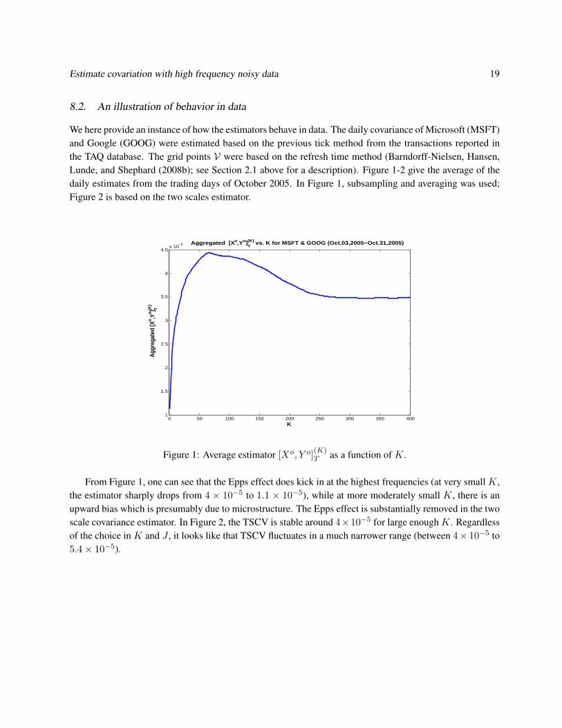
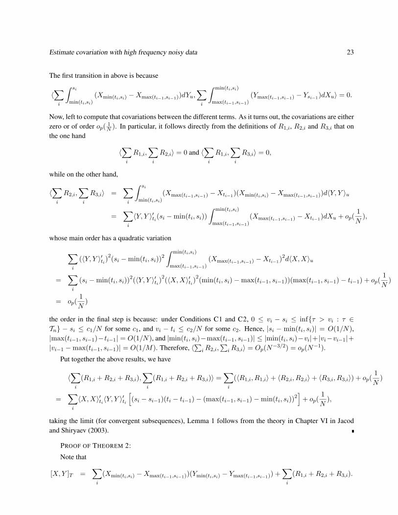
We here provide an instance of how the estimators behave in data. The daily covariance of Microsoft (MSFT)and Google (GOOG) were estimated based on the previous tick method from the transactions reported inthe TAQ database. The grid points V were based on the refresh time method (Barndorff-Nielsen, Hansen,Lunde, and Shephard (2008b); see Section 2.1 above for a description). Figure 1-2 give the average of thedaily estimates from the trading days of October 2005. In Figure 1, subsampling and averaging was used;Figure 2 is based on the two scales estimator.

0 50 100 150 200 250 300 350 4001

1.5

2

2.5

3

3.5

4

4.5x 10

−5 Aggregated [X o,Yo]T(K) vs. K for MSFT & GOOG (Oct.03,2005−Oct.31,2005)

Aggr

egat

ed [X

o ,Yo ] T(K

)

K

Figure 1: Average estimator [Xo, Y o](K)T as a function of K.

From Figure 1, one can see that the Epps effect does kick in at the highest frequencies (at very small K,the estimator sharply drops from 4 × 10−5 to 1.1 × 10−5), while at more moderately small K, there is anupward bias which is presumably due to microstructure. The Epps effect is substantially removed in the twoscale covariance estimator. In Figure 2, the TSCV is stable around 4×10−5 for large enoughK. Regardlessof the choice in K and J , it looks like that TSCV fluctuates in a much narrower range (between 4× 10−5 to5.4× 10−5).


0

5

10

15

20

0501001502002503003504003.8

4

4.2

4.4

4.6

4.8

5

5.2

5.4

x 10−5

J

Aggregated TSCV vs. K,J for MSFT & GOOG (Oct.03,2005−Oct.31,2005)

K

Aggr

egat

ed T

SCV

Figure 2: Two scales estimator 〈X,Y 〉T as a function of J and K.

9. Conclusion: the Epps effect and its remedies

This paper is about how to estimate 〈X,Y 〉T when the observation times of X and Y are not synchronizedand when the microstructure noise is present in the observed price processes. Using the previous-tick esti-mator for 〈X,Y 〉T , we show in Theorem 1 that for positively associated assetsX and Y , nonsynchronizationinduces a negative bias in the estimator. The magnitude of this bias increases in sampling frequency, up to apoint; On the other hand, it decreases for more liquid assets. This is an analytic characterization of the Eppseffect (Epps (1979)).

To cope with this effect, the paper offers two approaches. On the one hand, the effect can be controlledthrough a bias-variance trade-off. This trade-off provides a optimal scheme for subsampling observations.The scheme can incorporate microstructure noise.

A more satisfying approach is two- or multiscale estimation. Section 8 shows that this approach elimi-nates, at the same time, the biases due to asynchronicity and microstructure noise. The rate of convergenceis the same as that achieved in the scalar process case, where there is no asynchronicity.

The principles outlined can be applied similarly to multi scale estimation (Zhang (2006)), thus achievingrate efficiency. A full development of this approach is deferred to later work.


10. APPENDIX: PROOFS

PROOF OF THEOREM 1:

Assume first that µX = 0 and µY = 0. We know that the stochastic bias of [X,Y ]T is

MN∑i=1

∫ min(ti,si)

max(ti−1,si−1)〈X,Y 〉′udu− 〈X,Y 〉T =

∫ T

0〈X,Y 〉′ud[GN (u)− u],

where

GN (t) =∫ t

0

MN∑i=1

I(max(ti−1, si−1) < v < min(ti, si))dv

=∑

i:min(ti,si)≤t

(min(ti, si)−max(ti−1, si−1)) + (t− t)

=∑

i:min(ti,si)≤t

(min(ti, si)−max(ti−1, si−1)) +Op(1N

)

where t = max{l ∈ T ∪ S : l ≤ t}. Hence (11) follows since

GN (t)− t = −max(t1, s1)−∑

i:max(ti,si)≤t

(max(ti, si)−min(ti, si)),

= −∑

i:max(ti,si)≤t

(max(ti, si)−min(ti, si)) +Op(1N

).

To see why NMN

∫ T0 〈X,Y 〉

′tdFN (t) is RCP, note that under C2, 0 ≤ vi−ti ≤ inf{τ > vi : τ ∈ Tn}−ti ≤ c1

N

for some positive constant c1. Similarly, vi − si ≤ c2N for some positive constant c2.

Set 0 ≤ δti = N(vi − ti) ≤ c and set 0 ≤ δsi = N(vi − si) ≤ c for some c. Then,

N

MNFN (t) =

1MN

∑i:max(ti,si)≤t

[max(δti , δsi )−min(δti , δ

si )]

=1MN

∑i:vi≤t

[max(δti , δsi )−min(δti , δ

si )] + op(1) = Op(1).

Hence, NMN

FN (t) is RCP by Helly’s Theorem (Ash (1972), p 329). The same result for the stochastic biasfollows since 〈X,Y 〉′t is continuous.

If we do not assume that µX = 0 and µY = 0, it is easy to see that the contribution to the bias fromsuch terms is asymptotically negligible. To see this, we refer to Girsanov’s Theorem and the device used atthe beginning of the proof of Theorem 2 in Zhang, Mykland, and Aıt-Sahalia (2005) (Section A.3, p. 1410).This works unless the instantaneous correlation between X and Y is one. In this latter case, one should usethe methods of Mykland and Zhang (2006).

Lemma 1. Let X and Y be Ito processes satisfying (1)-(2). Let vi, ti, and si be the i-th sampling point, andthe previous ticks in X and in Y , respectively, as defined in Section 2.1. Let RN =

∑i(R1,i, R2,i and R3,i),


where

R1.i = (Xti −Xmin(ti,si))(Ysi − Ysi−1)

R2,i = (Xmax(ti−1,si−1) −Xti−1)(Ysi − Ysi−1)

R3,i = (Xmin(ti,si) −Xmax(ti−1,si−1))[(Ysi − Ymin(ti,si)) + (Ymax(ti−1,si−1) − Ysi−1)]

Then, under Conditions C1 and C2, U (nonsyn)N,u is RCP in the sense of Definition 3, and

RN = Op(1√N

), (41)

in particular, its quadratic variation

〈RN , RN 〉 =T

N

∫ T

0〈Y, Y 〉′u〈X,X〉′udU (nonsyn)

u + op(1N

), (42)

through any subsequence for which U (nonsyn)u (the limit of U (nonsyn)

N,u ) exists. 2

PROOF OF LEMMA 1:

U(nonsyn)N,u is RCP by the same methods as in the proof of Theorem 1.

Note that the leading terms in R1,i -R3,i are martingale increments, with order root N . This is because

〈∑i

R1,i,∑i

R1,i〉 =∑i

(Ysi − Ysi−1)2∫ ti

min(si,ti)d〈X,X〉u

=∑i

(〈Y, Y 〉si − 〈Y, Y 〉si−1)∫ ti

min(si,ti)d〈X,X〉u + op(

1N

)

=∑i

〈Y, Y 〉′si〈X,X〉′si(si − si−1)(ti −min(si, ti)) + op(

1N

).

Similarly,

〈∑i

R2,i,∑i

R2,i〉 =∑i

〈Y, Y 〉′si−1〈X,X〉′si−1

(max(ti−1, si−1)− ti−1)(si − si−1) + op(1N

).

At last, for∑

iR3,i:

〈R3,i, R3,i〉 =∑i

∫ si

min(ti,si)(Xmin(ti,si) −Xmax(ti−1,si−1))

2d〈Y, Y 〉u

+∑i

∫ min(ti,si)

max(ti−1,si−1)(Ymax(ti−1,si−1) − Ysi−1)2d〈X,X〉u

=∑i

〈X,X〉′ti〈Y, Y 〉′ti(min(ti, si)−max(ti−1, si−1))[(si −min(si, ti)) + (max(ti−1, si−1)− si−1)]

+ op(1N

)


The first transition in above is because

〈∑i

∫ si

min(ti,si)(Xmin(ti,si) −Xmax(ti−1,si−1))dYu,

∑i

∫ min(ti,si)

max(ti−1,si−1)(Ymax(ti−1,si−1) − Ysi−1)dXu〉 = 0.

Now, left to compute that covariations between the different terms. As it turns out, the covariations are eitherzero or of order op( 1

N ). In particular, it follows directly from the definitions of R1,i, R2,i and R3,i that onthe one hand

〈∑i

R1,i,∑i

R2,i〉 = 0 and 〈∑i

R1,i,∑i

R3,i〉 = 0,

while on the other hand,

〈∑i

R2,i,∑i

R3,i〉 =∑i

∫ si

min(ti,si)(Xmax(ti−1,si−1) −Xti−1)(Xmin(ti,si) −Xmax(ti−1,si−1))d〈Y, Y 〉u

=∑i

〈Y, Y 〉′ti(si −min(ti, si))∫ min(ti,si)

max(ti−1,si−1)(Xmax(ti−1,si−1) −Xti−1)dXu + op(

1N

),

whose main order has a quadratic variation

∑i

(〈Y, Y 〉′ti)2(si −min(ti, si))

2∫ min(ti,si)

max(ti−1,si−1)(Xmax(ti−1,si−1) −Xti−1)2d〈X,X〉u

=∑i

(si −min(ti, si))2(〈Y, Y 〉′ti)

2(〈X,X〉′ti)2(min(ti, si)−max(ti−1, si−1))(max(ti−1, si−1)− ti−1) + op(

1N

)

= op(1N

)

the order in the final step is because: under Conditions C1 and C2, 0 ≤ vi − si ≤ inf{τ > vi : τ ∈Tn} − si ≤ c1/N for some c1, and vi − ti ≤ c2/N for some c2. Hence, |si − min(ti, si)| = O(1/N),|max(ti−1, si−1)−ti−1| = O(1/N), and |min(ti, si)−max(ti−1, si−1)| ≤ |min(ti, si)−vi|+ |vi−vi−1|+|vi−1 −max(ti−1, si−1)| = O(1/M). Therefore, 〈

∑iR2,i,

∑iR3,i〉 = Op(N−3/2) = op(N−1).

Put together the above results, we have

〈∑i

(R1,i +R2,i +R3,i),∑i

(R1,i +R2,i +R3,i)〉 =∑i

(〈R1,i, R1,i〉+ 〈R2,i, R2,i〉+ 〈R3,i, R3,i〉) + op(1N

)

=∑i

〈X,X〉′ti〈Y, Y 〉′ti

[(si − si−1)(ti − ti−1)− (max(ti−1, si−1)−min(ti, si))

2]

+ op(1N

),

taking the limit (for convergent subsequences), Lemma 1 follows from the theory in Chapter VI in Jacodand Shiryaev (2003).

PROOF OF THEOREM 2:

Note that

[X,Y ]T =∑i

(Xmin(ti,si) −Xmax(ti−1,si−1))(Ymin(ti,si) − Ymax(ti−1,si−1)) +∑i

(R1,i +R2,i +R3,i).


Invoking Ito’s formula on the first term, we obtain,∑i

(Xmin(ti,si) −Xmax(ti−1,si−1))(Ymin(ti,si) − Ymax(ti−1,si−1))

=∑i

(〈X,Y 〉min(ti,si) − 〈X,Y 〉max(ti−1,si−1)) +∑i

∫ min(ti,si)

max(ti−1,si−1)(Xu −Xmax(ti−1,si−1))dYu[2]

=∑i

∫ min(ti,si)

max(ti−1,si−1)〈X,Y 〉′udu+

∑i

∫ min(ti,si)

max(ti−1,si−1)(Xu −Xmax(ti−1,si−1))dYu[2].

The asymptotic variance of [X,Y ]T has two components, one –∑

i(R1,i + R2,i + R3,i) – comes from thenonsynchronization, while the other –

∑i

∫ min(ti,si)max(ti−1,si−1)(Xu − Xmax(ti−1,si−1))dYu[2] – is because of the

discrete trading (or recording) time. The former is analyzed in Lemma 1. Now we are left to show the resultin the latter term and the interaction between the two terms.

We start with the quadratic variation of∑

i

∫ min(ti,si)max(ti−1,si−1)(Xu −Xmax(ti−1,si−1))dYu[2].

〈∑i

∫ min(ti,si)

max(ti−1,si−1)(Xu −Xmax(ti−1,si−1))dYu[2],

∑i

∫ min(ti,si)

max(ti−1,si−1)(Xu −Xmax(ti−1,si−1))dYu[2]〉

=∑i

∫ min(ti,si)

max(ti−1,si−1)(Xu −Xmax(ti−1,si−1))

2d〈Y, Y 〉u

+∑i

∫ min(ti,si)

max(ti−1,si−1)(Yu − Ymax(ti−1,si−1))

2d〈X,X〉u

+2∑i

∫ min(ti,si)

max(ti−1,si−1)(Xu −Xmax(ti−1,si−1))(Yu − Ymax(ti−1,si−1))d〈X,Y 〉u

=∑i

〈X,X〉′ti〈Y, Y 〉′ti(min(ti, si)−max(ti−1, si−1))2

+∑i

(〈X,Y 〉′ti)2(min(ti, si)−max(ti−1, si−1))2 +QN,T [2] + op(

1

M3/2N

),

where

QN,T [2] = 2∑i

〈X,X〉′ti

∫ min(ti,si)

max(ti−1,si−1)(min(ti, si)− u)(Yu − Ymax(ti−1,si−1))dYu[2]

+2∑i

〈X,Y 〉′ti

∫ min(ti,si)

max(ti−1,si−1)(min(ti, si)− u)(Xu −Xmax(ti−1,si−1))dYu[2].

By the results and the methods in Lemma 2 ( with αi = max(ti−1, si−1) and βi = min(ti, si)), we obtainthat the quadratic variation of QN [2] is as follows:

〈QN [2], QN [2]〉

=23

MN∑i=1

(min(ti, si)−max(ti−1, si−1))4

×{

(〈X,X〉′ti−1)2(〈Y, Y 〉′ti−1

)2 + 6(〈X,X〉′ti−1)(〈Y, Y 〉′ti−1

)(〈X,Y 〉′ti−1)2 + (〈X,Y 〉′ti−1

)4}× (1 + op(1)).


Under Condition C2, we know that QN,T [2] = Op( 1

M3/2N

).

By continuity, and using (13)∑i

〈X,X〉′ti〈Y, Y 〉′ti(min(ti, si)−max(ti−1, si−1))2 +

∑i

(〈X,Y 〉′ti)2(min(ti, si)−max(ti−1, si−1))2

∼ T

M

∫ T

0

[〈X,X〉′u〈Y, Y 〉′u + (〈X,Y 〉′u)2

]dU

(dis)N,u .

For a rigorous proof of similar statements under lesser regularity conditions, see Proposition 1 and Proposi-tion 3 in Mykland and Zhang (2006).

To see equation (13), let δsi and δti be as defined in the proof of Theorem 1, and set ∆v = T/MN . Wethen get that

min(ti, si)−max(ti−1, si−1) = ∆v −N−1(max(δti , δsi )−min(δti−1, δ

si−1)).

Hence,

U(dis)N,u =

MN

T

∑i:ti,si≤u

((∆v)2 − 2

∆vN

(max(δti , δsi )−min(δti−1, δ

si−1)) +O(N−2)

)= u− 2FN (u) +O(M−1

N ) +O((MN/N)2),

proving (13).

Next we study the interaction term. Since∑

i

∫ min(ti,si)max(ti−1,si−1)(Xu−Xmax(ti−1,si−1))dYu[2] is symmetric,

we only need to show the interaction between∑

i

∫ min(ti,si)max(ti−1,si−1)(Xu−Xmax(ti−1,si−1))dYu and

∑i(R1,i +

R2,i +R3,i). First, it is obvious that

〈∑i

∫ min(ti,si)

max(ti−1,si−1)(Xu −Xmax(ti−1,si−1))dYu,

∑i

R1,i〉 = 0.

For the rest, we have

〈∑i

∫ min(ti,si)


∑i

R2,i〉

=∑i

∫ min(ti,si)

max(ti−1,si−1)(Xu −Xmax(ti−1,si−1))(Xmax(ti−1,si−1) −Xti−1)d〈Y, Y 〉u

=∑i

(Xmax(ti−1,si−1) −Xti−1)∫ min(ti,si)

max(ti−1,si−1)〈Y, Y 〉′ti−1

(min(ti, si)− u)dXu × (1 + op(1)),

which has a quadratic variation∑i

(Xmax(ti−1,si−1) −Xti−1)2(〈Y, Y 〉′ti−1)2∫ min(ti,si)

max(ti−1,si−1)(min(ti, si)− u)2d〈X,X〉u × (1 + op(1))

≤ 13

supt

(〈Y, Y 〉′t)2 sup

t(〈X,X〉′t)

2∑i

(max(ti−1, si−1)− ti−1)(min(ti, si)−max(ti−1, si−1))3 × (1 + op(1))

= Op(1

NM2).


Hence

〈∑i

∫ min(ti,si)


∑i

R2,i〉 = Op(1√NM

).

By same method,

〈∑i

∫ min(ti,si)


∑i

R3,i〉 = Op(1√NM

).

In sum, the interaction term is negligible. Theorem 2 is proved.

For next Lemma, we use the notation∫XdY [2] =

∫XdY +

∫Y dX .

Lemma 2. Let X and Y be Ito processes satisfying (1)-(2). Let N and MN be as defined in Section 2.1.Denote

QN = 2MN∑i=1

〈Y, Y 〉′αi

∫ βi

αi

(βi − u)(Xu −Xαi)dXu,

and

RN =MN∑i=1

〈X,Y 〉′αi

∫ βi

αi

(βi − u)(Xu −Xαi)dYu[2].

Assuming Condition C1, then

MN∑i=1

∫ βi

αi

(Xu −Xαi)2d〈Y, Y 〉u =

12

MN∑i=1

〈X,X〉′αi〈Y, Y 〉′αi(βi − αi)

2 +QN + op(1

M3/2N

),

where QN has quadratic variation

13

MN∑i=1

(〈X,X〉′αi)2(〈Y, Y 〉′αi)

2(βi − αi)4 × (1 + op(1)).

Similarly,

MN∑i=1

∫ βi

αi

(Xu −Xαi)(Yu − Yαi)d〈X,Y 〉u =12

MN∑i=1

(〈X,Y 〉′αi)2(βi − αi)2 +RN + op(

1

M3/2N

),

where RN has quadratic variation

16

MN∑i=1

(〈X,Y 〉′αi)2(〈X,X〉′αi)(〈Y, Y 〉

′αi)(βi − αi)

4 × (1 + op(1)).

PROOF OF LEMMA 2:

We first show that

〈∫ βi

αi

∫ u

αi

(Xv −Xαi)dXvdu,

∫ βi

αi

∫ u

αi

(Xv −Xαi)dXvdu〉 =112

(〈X,X〉′αi)2(βi − αi)4 × (1 + op(1)). (43)


Use integration by parts on the outer integration, we get∫ βi

αi

∫ u

αi

(Xv −Xαi)dXvdu = (βi − αi)∫ βi

αi

(Xu −Xαi)dXu −∫ βi

αi

(u− αi)(Xu −Xαi)dXu

=∫ βi

αi

(βi − u)(Xu −Xαi)dXu,

which has quadratic variation∫ βi

αi

(βi − u)2(Xu −Xαi)2d〈X,X〉u =

∫ βi

αi

(βi − u)2(〈X,X〉u − 〈X,X〉αi)d〈X,X〉u × (1 + op(1))

= (〈X,X〉′αi)2∫ βi

αi

(βi − u)2(u− αi)du× (1 + op(1))

=112

(〈X,X〉′αi)2(βi − αi)4 × (1 + op(1))

Next, invoke Ito’s formula,

MN∑i=1

∫ βi

αi

(Xu −Xαi)2d〈Y, Y 〉u

=MN∑i=1

〈Y, Y 〉′αi

∫ βi

αi

(Xu −Xαi)2du+ op(M

−3/2N )

=MN∑i=1

〈Y, Y 〉′αi

∫ βi

αi

(〈X,X〉u − 〈X,X〉αi)du+ 2MN∑i=1

〈Y, Y 〉′αi

∫ βi

αi

∫ u

αi

(Xv −Xαi)dXvdu+ op(M−3/2N )

=12

MN∑i=1

〈X,X〉′αi〈Y, Y 〉′αi(βi − αi)

2 +QN + op(M−3/2N ) by (43)

Similarly,

MN∑i=1

∫ βi

αi

(Xu −Xαi)(Yu − Yαi)d〈X,Y 〉u

=MN∑i=1

〈X,Y 〉′αi

∫ βi

αi

(Xu −Xαi)(Yu − Yαi)du+ op(M−3/2N )

=MN∑i=1

〈X,Y 〉′αi

∫ βi

αi

(〈X,Y 〉u − 〈X,Y 〉αi)du+MN∑i=1

〈X,Y 〉′αi

∫ βi

αi

(∫ u

αi

(Xv −Xαi)dYv[2])du+ op(M

−3/2N )

=12

MN∑i=1

(〈X,Y 〉′αi)2(βi − αi)2 +RN + op(M

−3/2N )

PROOF OF THEOREM 4. Since in this case, U (nonsyn)N,t → 0, it follows from the proof of Theorem

2 that we can take LN in Theorem 3 to be∑

i

∫ min(ti,si)max(ti−1,si−1)(Xu − Xmax(ti−1,si−1))dYu[2]. Now set


LN =∑

i

∫ max(ti,si)max(ti−1,si−1)(Xu − Xmax(ti−1,si−1))dYu[2]. To assess LN − LN =

∑i

∫ max(ti,si)min(ti,si))

(Xu −Xmax(ti−1,si−1))dYu[2], note that

〈∑i

∫ max(ti,si)

min(ti,si)(Xu −Xmax(ti−1,si−1))dYu,

∑i

∫ max(ti,si)

min(ti,si)(Xu −Xmax(ti−1,si−1))dYu〉

=∑i

∫ max(ti,si)

min(ti,si)(Xu −Xmax(ti−1,si−1))

2d〈Y, Y 〉u

=∑i

〈X,X〉′max(ti−1,si−1)〈Y, Y 〉′min(ti,si)

∫ max(ti,si)

min(ti,si)(u−max(ti−1, si−1))du(1 + op(1))

≤ 1N

∫ T

0〈X,X〉′t〈Y, Y 〉′tdt

= Op(1/N),

and similarly for the second term. This shows the result for wi = max(ti, si). The result for vi followssimilarly.

PROOF OF COROLLARY 2: To show equation (21), define δti and δsi as in the proof of Theorem 1. Wethen obtain that (with ∆v = T/MN )

N

T

∑i:si,ti≤u

(si − si−1)(ti − ti−1)

=N

T

∑i:si,ti≤u

((∆v)2 −N−1∆v(δsi − δsi−1)−N−1∆v(δti − δti−1) +N−2(δsi − δsi−1)(δti − δti−1))

=N

T

∑i:si,ti≤u

(∆v)2 + o(1) (44)

(by telescope sum) and

N

T

∑i:si,ti≤u

(max(ti−1, si−1)−min(ti, si))2

=N

T

∑i:si,ti≤u

((∆v)2 − 2N−1∆v(max(δsi , δti)−min(δsi−1, δ

ti−1))) + o(1)

=N

T

∑i:si,ti≤u

(∆v)2 − 2N

MNFN (u) + o(1) (45)

Since U (nonsyn)N,u is defined as the difference between the two above terms, the result (21) follows.

PROOF OF THEOREM 5. The proof is similar to that of the earlier results; the main difference lies inverifying that the relevant sequences are RCP in the sense of Definition 3. We here provide the argument inthe case of the bias; entirely similar considerations apply to the variance.

Consider first the term

α

Mα

∑i

(vi −max(si, ti)) ≤α

Mα

∑i

(vi − si) +α

Mα

∑i

(vi − ti) (46)


Suppose one considers the following subsampling scheme: every time τi occurs, it is sampled with proba-bility cα/λXα (τi). By standard considerations, the subsampled times τ ′i are derived from a Poisson processwith intensity cα. Suppose that the number of such τ ′i is n′. If t′i = max{τ ′j ≤ vi} one obtains that

α

Mα

∑i

(vi − ti) ≤α

Mα

∑i

(vi − t′i) (47)

Note that by the Poisson property of the τ ′i , the expectation of the right hand side of (47) is bounded by 1/c,hence (47) is Op(1). By using the same argument on the sis, one thus obtains that (46) is Op(1). Finally, ifN ′ = m′ + n′, by the law of large numbers, N ′/α→ 2cT as α→∞. Hence N

MNFN (T ) is Op(1). Again,

by Helly’s Theorem (Ash (1972), p. 329), NMN

FN (t) is RCP. The rest of the proof follows similarly.

PROOF OF COROLLARY 4:

Let vi, si, and ti be the same as in Section 2.1. Since X and Y are Poisson with intensities λXα and λYα ,respectively, we get vi − ti ∼ exp(λXα )2, and vi − si ∼ exp(λYα ), thus

vi −max(ti, si) = min ((vi − ti), (vi − si)) ∼ exp(λXα + λYα ).

Also, since

vi −min(ti, si) = max (vi − ti, vi − si)= (vi − ti) + (vi − si)−min (vi − ti, vi − si)∼ exp(λXα ) + exp(λYα )− exp(λXα + λYα ) (48)

then,

FN (vk) = −k∑i=1

[−(vi −min(ti, si)) + (vi −max(ti, si))] +Op(1N

). (49)

Under our assumptions,

E[FN (vk)] = −k(− 1λXα− 1λYα

+2

λXα + λYα) +O(

1α

).

Also note thatN/(λXα T +λYαT )→ 1 in probability. By appropriate normalization, it follows that (31) holdsin expectation. By observing that (49) is an independent sum, it also follows that (31) holds in probability.Thus, (32) yields accordingly.

PROOF OF COROLLARY 5:

This is a direct consequence of Theorem 2 and Corollaries 2 and 4. We here provide an independentproof as an addition. Again use the relation (48), we obtain

E[vi −min(ti, si)|vi] =1λXα

+1λYα− 1λXα + λYα

, (50)

2X ∼ exp(λ) means X follow exponential distribution with intensity λ.


and

E[((min(ti, si)− vi)2|vi)

]=

2

(λXα )2+

2

(λYα )2+

2

(λXα + λYα )2+

2λXα λ

Yα

− 2E[(vi − ti) min(vi − ti, vi − si)|vi][2]

=2

(λXα )2+

2

(λYα )2+

2

(λXα + λYα )2− 2λXα λ

Yα

+2

(λXα + λYα )2(λXαλYα

+λYαλXα

) (51)

where E[(vi − ti) min(vi − ti, vi − si)|vi][2] = E[((vi − ti) + (vi − si)) min(vi − ti, vi − si)|vi]. The firststep is due to the independence between X and Y , and the second step is because

E[(vi − si) min(vi − ti, vi − si)|vi] = −λYα

λXα

1

(λXα + λYα )2+

1λXα λ

Yα

.

Thus, by independent increment and by (50)-(51), we get

E[(min(ti, si)−max(ti−1, si−1))2|vi]= E[((min(ti, si)− vi) + (vi − vi−1) + (vi−1 −max(ti−1, si−1))2|vi]

= (T

Mα)2{

1 + 2Mα

T

(2

λXα + λYα− 1λXα− 1λYα

)}+O(

1α2

).

Therefore,

EU(dis)N,vk

= kT

Mα

[1 + 2

Mα

T(

2λXα + λYα

− 1λXα− 1λYα

) +O(1α2

)].

Similarly, E[(si − si−1)] = E[(si − vi) + (vi − vi−1) + (vi−1 − si−1)|vi] = TMα

= E[(ti − ti−1)|vi], thus,

E(U (nonsyn)N,vk

) = 2(λXα + λYα )k[T

Mα(− 2λXα + λYα

+1λXα

+1λYα

) +O(1α2

)].

By the same argument as in the proof of Corollary 4 and the results in Theorem 2, the asymptotic stochasticvariance due to discretization is

T

Mα

∫ T

0(〈X,Y 〉′u)2 + 〈X,X〉′u〈Y, Y 〉′udu− 2

T

N

(`Y

`X+`X

`Y

)∫ T

0(〈X,Y 〉′u)2 + 〈X,X〉′u〈Y, Y 〉′udu,

whereas the the asymptotic stochastic variance due to nonsynchonization is

2T

N

∫ T

0〈X,X〉′u〈Y, Y 〉′udu

(`Y

`X+`X

`Y

)Adding up, (33) follows by the law of large numbers.

PROOF OF THEOREM 6: Consider separately the signal and noise terms in (39). This is legitimate sincethe two terms are independent. It is easy to see that the term involving the semimartingales X and Y ishandled exactly in analogy with the similar development (Theorem 3) in Zhang, Mykland, and Aıt-Sahalia(2005), integrating the methodology from Theorem 2 in the current paper. The constant appears as follows:the constant c from the earlier paper is here c ∼ KN/M

2/3N ∼ c2c−2/3

1 .


For the noise term, replace normalization by N1/6/KN by M−1/2N (thus creating a constant of c1/21 c−1

2 ,which is squared in the variance). We now have to deal with two suitably normalized mixing sums. Theasymptotic normality follows as in Chapter 5 of Hall and Heyde (1980). It is easy to verify that the two sumsare asymptotically uncorrelated. If one sets γi,j = Cov(εXt0 ε

Ys−j [2], εXti ε

Ysi−j [2]), the asymptotic variance of

the “J” term thus gets the form γ0,J + 2∑∞

i=1 γi,J , and similarly for the “K” term (let J → ∞ is it isn’talready there). To see the expression for γi,j , note that

γi,j = Cov(εXt0 εYs−j + εYs0ε

Xt−j , ε

Xti ε

Ysi−j + εYsiε

Xti−j )

= 2Cov(εXt0 , εXti )Cov(εYs0 , ε

Ysi) + 2Cov(εXt0 , ε

Ysi)Cov(εYs0 , ε

Xti )

+ Cov(εXt0 , εYsi−j )Cov(εYs−j , ε

Xti ) + Cov(εYs0 , ε

Xti−j )Cov(εXt−j , ε

Ysi)

+ Cov(εXt0 , εXti−j )Cov(εYs−j , ε

Ysi) + Cov(εYs0 , ε

Ysi−j )Cov(εXti , ε

Xt−j )

+ cum(εXt0 , εXti , ε

Ys−j , ε

Ysi−j ) + cum(εYs0 , ε

Ysi , ε

Xt−j , ε

Xti−j )

+ cum(εXt0 , εXti−j , ε

Ys−j , ε

Ysi) + cum(εXti , ε

Xt−j , ε

Ys0 , ε

Ysi−j ) (52)

Obviously, as j →∞, γi,j tends to the expression in (40).

REFERENCES

Aıt-Sahalia, Y., Mykland, P. A., Zhang, L., 2005. How often to sample a continuous-time process in thepresence of market microstructure noise. Review of Financial Studies 18, 351–416.

Aıt-Sahalia, Y., Mykland, P. A., Zhang, L., 2009. Ultra high frequency volatility estimation with dependentmicrostructure noise. Tech. rep., in revision for JOE.

Aldous, D., 1989. Probability Approximations via the Poisson Clumping Heuristic. Springer-Verlag.

Aldous, D. J., Eagleson, G. K., 1978. On mixing and stability of limit theorems. Annals of Probability 6,325–331.

Andersen, T. G., Bollerslev, T., 1998. Answering the skeptics: Yes, standard volatility models do provideaccurate forecasts. International Economic Review 39, 885–905.

Andersen, T. G., Bollerslev, T., Diebold, F. X., Labys, P., 2001. The distribution of realized exchange ratevolatility. Journal of the American Statistical Association 96, 42–55.

Ash, R. B., 1972. Real Analysis and Probability. Academic Press.

Barndorff-Nielsen, O. E., Hansen, P. R., Lunde, A., Shephard, N., 2008a. Designing realized kernels tomeasure ex-post variation of equity prices in the presence of noise. Econometrica 76, 1481–1536.

Barndorff-Nielsen, O. E., Hansen, P. R., Lunde, A., Shephard, N., 2008b. Multivariate realised kernels:Consistent positive semi-definite estimators of the covariation of equity prices with noise and non-synchronous trading. Tech. rep., University of Oxford.

Barndorff-Nielsen, O. E., Hansen, P. R., Lunde, A., Shephard, N., 2009. Subsampling realised kernels.Journal of Econometrics, forthcoming .


Barndorff-Nielsen, O. E., Shephard, N., 2002a. Econometric analysis of realized volatility and its use inestimating stochastic volatility models. Journal of the Royal Statistical Society, B 64, 253–280.

Barndorff-Nielsen, O. E., Shephard, N., 2002b. Estimating quadratic variation using realised variance. Jour-nal of Applied Econometrics 17, 457–477.

Dacorogna, M. M., Gencay, R., Muller, U., Olsen, R. B., Pictet, O. V., 2001. An Introduction to High-Frequency Finance. Academic Press, San Diego.

Delattre, S., Jacod, J., 1997. A central limit theorem for normalized functions of the increments of a diffusionprocess, in the presence of round-off errors. Bernoulli 3, 1–28.

Devroye, L., 1981. Law of the iterated logarithm for order statistics for uniform spacing. Annals of Proba-bility 9, 860–867.

Devroye, L., 1982. A log log law for maximal uniform spacings. Annals of Probability 10, 863–868.

Epps, T. W., 1979. Comovements in stock prices in the very short run. Journal of the American StatisticalAssociation 74, 291–298.

Gencay, R., Ballocchi, G., Dacorogna, M., Olsen, R., Pictet, O., 2002. Real-time trading models and thestatistical properties of foreign exchange rates. International Economic Review 43, 463–491.

Griffin, J., Oomen, R., 2007. Covariance measurement in the presence of non-synchronous trading andmarket microstructure noise, preprint.

Hall, P., Heyde, C. C., 1980. Martingale Limit Theory and Its Application. Academic Press, Boston.

Jacod, J., Li, Y., Mykland, P. A., Podolskij, M., Vetter, M., 2009. Microstructure noise in the continuouscase: The pre-averaging approach. Stochastic Processes and Their Applications 119, 2249–2276.

Jacod, J., Protter, P., 1998. Asymptotic error distributions for the euler method for stochastic differentialequations. Annals of Probability 26, 267–307.

Jacod, J., Shiryaev, A. N., 2003. Limit Theorems for Stochastic Processes, 2nd Edition. Springer-Verlag,New York.

Lo, A. W., MacKinlay, A. C., 1990. An econometric analysis of nonsynchronous trading. Journal of Econo-metrics 45, 181–211.

Lunde, A., Voev, V., 2007. Integrated covariance estimation using high-frequency data in the presence ofnoise. Journal of Financial Econometrics 5, 68–104.

McCullagh, P., 1987. Tensor Methods in Statistics. Chapman and Hall, London, U.K.

Mykland, P. A., 1994. Bartlett type identities for martingales. Annals of Statistics 22, 21–38.

Mykland, P. A., Zhang, L., 2006. ANOVA for diffusions and Ito processes. Annals of Statistics 34, 1931–1963.

Podolskij, M., Vetter, M., 2009. Estimation of volatility functionals in the simultaneous presence of mi-crostructure noise and jumps. Bernoulli, forthcoming .

Renyi, A., 1963. On stable sequences of events. Sankya Series A 25, 293–302.


Rootzen, H., 1980. Limit distributions for the error in approximations of stochastic integrals. Annals ofProbability 8, 241–251.

Ross, S., 1996. Stochastic Processes, 2nd Edition. Wiley, New York, N.Y.

Scholes, M., Williams, J., 1977. Estimating betas from nonsynchronous data. Journal of Financial Eco-nomics 5, 309–327.

Shorack, G. R., Wellner, J. A., 1986. Empirical Processes with Application to Statistics. Wiley.

Zhang, L., 2001. From martingales to ANOVA: Implied and realized volatility. Ph.D. thesis, The Universityof Chicago, Department of Statistics.

Zhang, L., 2006. Efficient estimation of stochastic volatility using noisy observations: A multi-scale ap-proach. Bernoulli 12, 1019–1043.

Zhang, L., Mykland, P. A., Aıt-Sahalia, Y., 2005. A tale of two time scales: Determining integrated volatilitywith noisy high-frequency data. Journal of the American Statistical Association 100, 1394–1411.

Zhang, L., Mykland, P. A., Aıt-Sahalia, Y., 2009. Edgeworth expansions for realized volatility and relatedestimators. Tech. rep., University of Illinois at Chicago.

estimating covariation: epps effect, microstructure noise · estimate covariation with high...

Documents