estimating components of variation in flight times

1

Estimating Components of Variation in Flight Times

Thomas R. Willemain, Ph.D.

Distinguished Visiting Professor, Federal Aviation Administration

and

Professor, Department of Decision Sciences and Engineering Systems

Rensselaer Polytechnic Institute

May 21, 2001

NEXTOR WP-01-2

2

Abstract

The time to fly between two airports can vary significantly from day to day and flight to flight.

This variability is an indication of possible operational problems, because flight times should

ideally be very consistent. Some of the variation is systemic in origin, caused either by weather or

by en route or terminal area congestion. The remaining variation is idiosyncratic and attributable

to factors within an airline s control, such as route planning. It is of interest to the FAA to

estimate the systemic component of variability because the FAA is responsible for the

expeditious (and safe) movement of traffic. We study two types of daily variations in average

point-to-point air times: variations around long-run average air times, and deviations from

estimated times en route filed in flight plans. This analysis decomposes variations in air time into

four components: day (system-wide) effects, origin (departure airport) effects, destination (arrival

airport) effects, and residual (en route) effects. We illustrate the methodology with data for

afternoon air times in the eastern US. The methodology uncovered interesting relationships

within and between origin, destination, and en route effects. It can be used to focus attention on

times and airspaces impeding consistent flight and to provide the basis for a graphical display of

airspace problems.

3

1. Introduction

How long does it take to fly from Atlanta to Chicago? One answer to the question is an

air time (i.e., time from wheels off the ground to wheels on the ground) of 95 minutes, which is

the average for a large number of flights in early 2001.

For an individual flight, the air time depends on many factors, including winds aloft,

weather at the airports, congestion in the terminal airspace and along the air routes, type of

aircraft, policies of the airline (e.g., allowing land and hold short -- LAHSO -- operations on

intersecting runways), and objectives of the pilot (e.g., saving fuel versus saving time versus

avoiding turbulence). We consider the first three factors systemic, i.e., part of the environment

into which the flight ventures. We consider the last three factors idiosyncratic, i.e., specific to the

flight. Collectively, these sources of variation can generate significant differences from the

average air time: one flight from Atlanta to Chicago required 173 minutes, another only 78

minutes.

Both passengers and airlines value predictability, especially when passengers must make

connections from one flight to another. For this reason alone, it would be useful to monitor air

times as a daily indicator of the health of the national airspace system (NAS). While the

necessary data are collected continuously, they are not routinely analyzed for this purpose. Even

more helpful than simply plotting air times would be partitioning the variation so that the Federal

Aviation Administration (FAA) would know where to focus its efforts on reducing delays.

We outline below a method to accomplish this partitioning. The method is premised on

the obvious idea that systemic factors manifest themselves by affecting multiple flights and can

be estimated using some form of average across flights.

Consider a set of airports. If, on a particular day, the average air time for all flights

arriving at one of the airports is longer than expected, that is suggestive of a problem in the

arrival airspace of that airport. (An alternative explanation is that there are problems in the en

route airspace from all or most of the origin airports.) Similarly, if all flights leaving a particular

4

airport take longer than expected to fly to their destinations, this suggests a problem in the

departure airspace of that particular airport. If only flights between certain airports take longer

than expected, this suggests a problem in the en route airspace connecting them. Finally, if all

flights on a given day take longer than expected, this indicates a region-wide problem involving

all airports. We define the expected air time as either the average of a number of recent flights or

the estimated time en route (ETE) filed in the flight plan.

Note that we focus on air times. We exclude any times related to pushing back from the

gate and taxiing. The method could also be applied to gate-to-gate times, though we did not do so

here since we did not have access to that data.

2. Method for Analysis of Variation in Air Times between Origin-Destination Pairs

We base the analysis on daily average air times between origin-destination (OD) pairs.

There are two variants of the methodology, one using variations around long-run average air

times, the other using deviations from estimated times en route (ETEs) in filed flight plans. The

analyses in sections 2 and 3 use the former, while section 4 uses the latter.

For any OD pair observed over a number of days, there is an average air time, which

depends primarily on the distance between the two airports. In the short run, this average is of

little interest; rather, we focus on daily deviations around the average. These deviations indicate

inconsistency in air times, so it is useful to trace the source of these inconsistencies. To do so, we

create a sequence of two-way tables, one per day. Each day s table has rows for origin airports

and columns for destination airports. The datum in each cell of the table is the difference between

that day s average air time and the long-run average air time for that OD pair. Schematically, the

model for any given day decomposes the deviations into four components in a simple additive

model:

Deviation from Average Air Time for OD pair =

Day Effect + Origin Effect + Destination Effect + En Route Effect

5

(An alternative model specification would include interaction terms. However, this would

complicate matters and require more parameter estimates, worsening the consequences of missing

data. Furthermore, we have not seen evidence for interaction effects.)

We estimate the first three effects, leaving the en route effects as residual values. The day

effect represents a kind of overall average for that day s deviations. A large value here indicates

problems throughout the region containing the OD pairs. Origin effects represent contributions to

air time associated with the departure airports. A large value here indicates a problem with flights

leaving from the airport associated with that row of the table. Likewise, destination effects

represent contributions associated with arrival airports. Large values arise when columns contain

large positive values and indicate problems with the arrival airports. After fitting the deviations

using the day, origin and destination effects, the residuals are interpreted as en route effects.

Large residuals suggest delays in the airspace between particular OD pairs.

Given a two way table with an average value in each cell, a simple way to obtain

numerical estimates of effects is row+column analysis (Mosteller and Tukey 1977), which works

from averages for the entire data table, each row, and each column. This is essentially a two-way

analysis of variance (ANOVA) without interactions. However, row+column analysis, because it

uses averages, can be greatly distorted by a few outlier cells. A variant known as median polish

does a better job of isolating the effects of unusual events (Emerson and Hoaglin 1983). Median

polish uses medians rather than means for summaries, making the summaries resistant to outliers,

which then stand out better among the residuals. Both approaches, however, are affected by the

presence of holes in a table, i.e., cells with no data. Our tables have holes along the main

diagonal, since we do not analyze flights from, say, Boston to Boston. We also have holes in a

few other cells, corresponding to OD pairs with little traffic (e.g., Newark to LaGuardia). Holes

require extra iterations for the calculations and produce estimates lacking a property that we think

is desirable: the sum of origin effects should equal zero, as should the sum of destination effects.

6

In the end, to achieve resistance to outliers, deal with holes, and achieve estimates that

sum to zero, we estimated effects by solving a nonlinear programming problem. That is, we

minimized the sum of absolute values of the residuals from the fitted additive model, subject to

constraints that the origin and destination effects each sum to zero. We implemented these

calculations in Excel using the Solver add-in. These calculations are iterative and fairly

insensitive to the starting values, though the calculations go faster with good starting values. The

estimates produced by row+column analysis serve well as initial values. That is, the initial

estimate of the day effect is simply the average of all the deviations in the table. The estimates of

row or column effects are just the row or column averages less the table average.

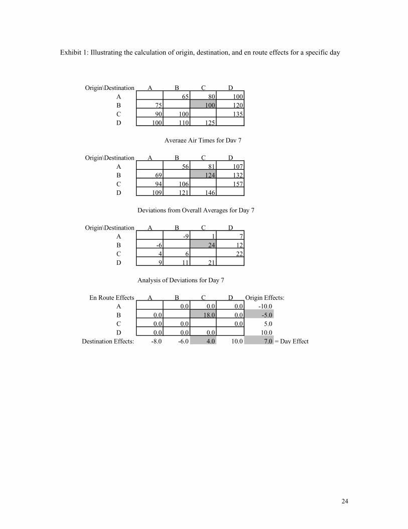
Exhibit 1 illustrates the decomposition of average air times for one day using artificial

data for four airports. Analysis begins with the first table, showing point-to-point air times

averaged over some period of time, say the 60 most recent days. For instance, the average air time

from B to C was 100 minutes. The second table shows the average air times for day 7, a day when

the average air time for flights from B to C happened to be 124 minutes. The third table expresses

the averages for day 7 as deviations from their long-term averages. This critical step puts all the

OD pairs on an equal footing, allowing us to combine results across airports. (Actually, this step

puts all OD pairs on an almost equal footing. Subtracting the long-term average value for each

cell does indeed set the expected values of all cells to zero. However, since longer air times also

tend to be more variable, the standard deviations still vary somewhat from cell to cell. We do not

believe this heteroscedasticity causes major estimation problems, and adjusting for it would

complicate the method. In section 6, we consider this and other technical problems with

estimation of effects.)

In the example, the average air time from B to C on day 7 was 24 minutes above the

long-run average for those flights. The final table in Exhibit 1 shows the estimated effects

computed from the deviations for day 7. The overall estimate for the table of deviations is 7,

indicating that day 7 as a whole had air times about 7 minutes longer than usual. The estimated

7

origin and destination effects are shown at the edges of the table. Flights leaving from airport B

had an average of 5 minutes less air time than the overall daily average. Flights arriving at airport

C had an average air time 4 minutes above the overall daily average. Thus, the model estimates

the deviation for flights from B to C to be 6 = 7 — 5 + 4. Comparing this fit to the observed

deviation of 24 gives a residual of 18 = 24 — 6. We attribute this additional 18 minutes to delays

en route.

We repeat this analysis for every day over the period of interest. If we have 60 days of

data, we end up with 60 consecutive estimates of each of the following quantities: the day effect,

the origin effect for each airport, the destination effect for each airport, and the en route effect for

each pair of airports. These sequences of estimated values can then be analyzed in their own right.

Unusually large values for any estimated effect indicate a problem. Furthermore, these estimates

can be correlated with each other to reveal patterns in the overall operation of the system.

The data in Exhibit 1 were contrived to be easy to analyze and interpret. Actual data

tables are larger and more complex. As mentioned above, real tables can have holes not only on

the main diagonal but also off it. The number of flights per day differs across OD pairs and within

OD pairs by day of the week, so different cell means have different standard errors. A more

elaborate treatment would take account of this sampling variability, but at the risk of losing

connection with the intended audience of FAA and airline staff.

One should design a table of air times with several objectives in mind. It is good for a

table to include many OD pairs, but not at the cost of containing many cells populated with few

or no flights. The condition of the NAS varies by time of day, so it is best for diagnostic purposes

to work only with flights from a portion of a day (say, morning, afternoon or evening flights). It is

also desirable to select OD pairs with a wide geographical dispersion to better sample the network

of airways.

8

3. Analysis of Afternoon Air Times in the Eastern US

To show the practical application of this methodology to assessing airborne delays in the

NAS, we used the POET software (POET 2001) to extract a large amount of information from the

FAA s Enhanced Traffic Management System (ETMS) database (ETMS 2001). The data were

actual air times (as recorded in ETMS as wheels on time minus wheels off time) between 10

airports, selected for their high levels of traffic as well as geographic coverage of the eastern US.

The flights in question had actual departure dates during the period January 29 to March 27, 2001

(except for March 10 and March 23, for which ETMS data were unavailable to POET). Since

conditions in the NAS change throughout the day, we selected only flights whose actual departure

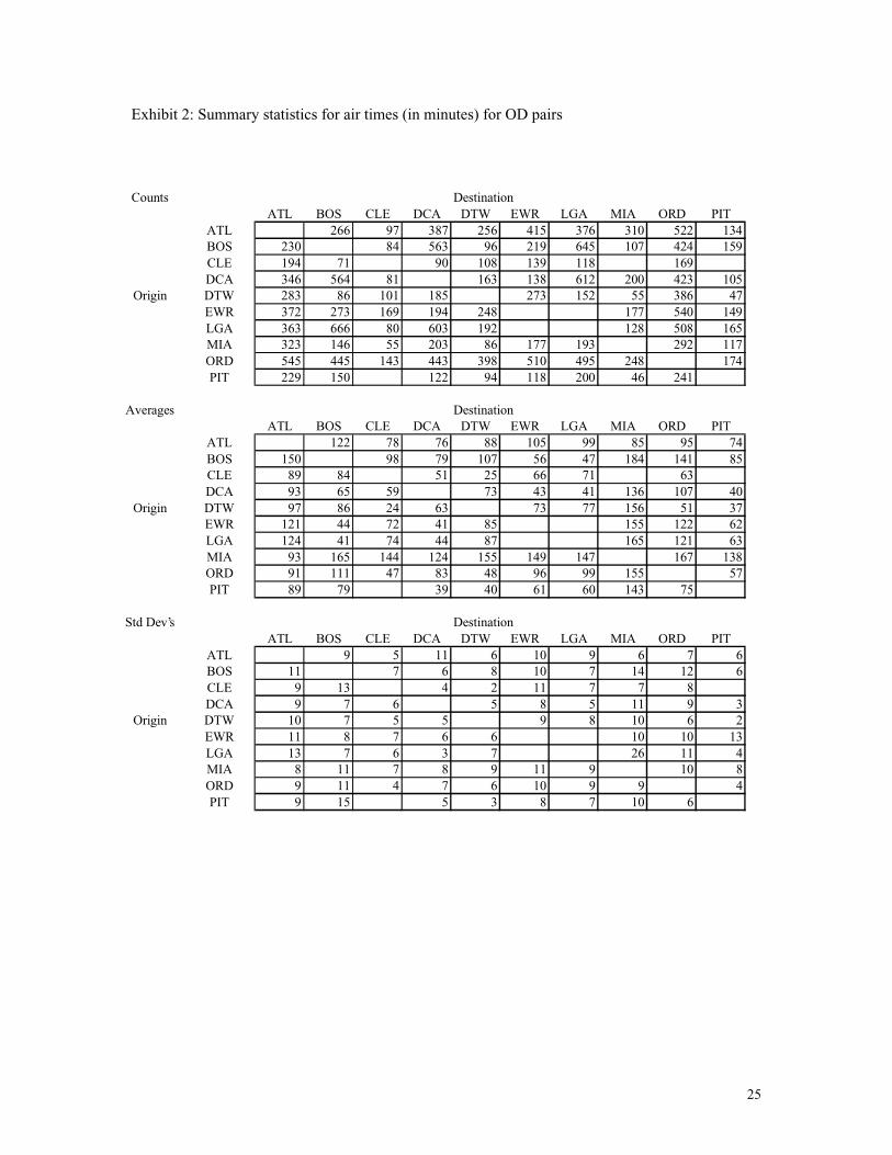
times were between 1700 and 2300 UTC, i.e., afternoon flights. We analyzed 21,399 flights by

the eight major airlines operating extensively in the eastern US at the time: American,

Continental, Delta, Northwest, Southwest, Trans World, United, and US Air. This focus on major

carriers minimized the confounding effects of different classes of aircraft on air times by

eliminating turboprops and regional jets from the dataset. (An additional 601 flights were

recorded in the dataset, but incomplete data excluded them from our analysis. Another 16 flights

were set aside either because they had the same origin and destination or because they were for an

OD pair with very few flights.). Summary statistics for the 21,339 flights are shown in Exhibit 2.

The distributions of the estimated day, destination, and origin effects are shown in

Exhibit 3. Of the 21 distributions of estimated effects, only 5 had no outliers, so there were a

number of days when estimated effects were especially interesting. At the same time, the number

of outliers was not so large as to overwhelm any effort to understand their causes. The lengths of

the boxplots indicate the daily variability in the estimated effects. From this perspective, the most

variable airports were Miami (MIA), Atlanta (ATL), Boston (BOS) and Chicago (ORD). (It is

worth noting that flights from Miami and Atlanta generally traveled the longest distances, which

tended to increase their variability. Therefore, some of the greater volatility of estimated effects

9

for these two airports might be attributed solely to this geographic factor.) We now examine the

estimated effects in some detail.

3.1 Day Effects

The single most inclusive indicator of the day to day variation in air times is the day

effect. Exhibit 4 plots estimated day effects. The day effect bobbed about more or less randomly.

The worst day was February 5, which was an outlier in a formal statistical sense. The additive

model attributes nearly 7 additional minutes to all air times on this day.

3.2 Origin Effects

Origin effects apply to all flights leaving from a given departure airport. Positive values

indicate contributions to longer air times. These might be caused by routing aircraft over

inconvenient departure fixes or placing speed or direction restrictions on departing flights to

maintain separation. Exhibit 5 shows estimated origin effects for Atlanta (ATL) and Miami

(MIA). On four days (February 5 and March 6, 21 and 22) flights leaving Atlanta had about 8

minutes additional air time. On March 6, flights leaving Miami had about 20 minutes additional

air time, whereas two days earlier, they enjoyed a reduction of about 12 minutes.

3.3 Destination Effects

Destination effects apply to all flights arriving at a given airport. Positive values indicate

contributions to longer air times. These might be traced to unfavorable runway configurations or

visibility or to maneuvers to increase spacing, such as extended downwind legs. Exhibit 6 shows

estimated destination effects for Detroit (DTW) and Boston (BOS). On February 5, flights

arriving in Detroit had about 8 minutes less than the expected air time. Boston, on the other hand,

recorded several good and bad days, notably the outlier on February 9, when the destination

effect added 16 minutes of air time.

3.4 En Route Effects

Deviations not traceable to the day, origin, or destination are, by default, attributed to the

en route phase of a flight. Factors influencing en route times include winds aloft, choice of flight

10

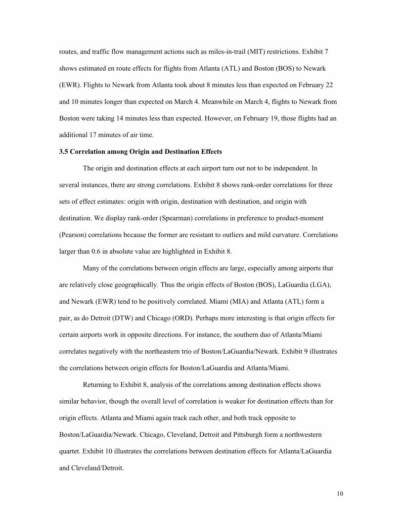
routes, and traffic flow management actions such as miles-in-trail (MIT) restrictions. Exhibit 7

shows estimated en route effects for flights from Atlanta (ATL) and Boston (BOS) to Newark

(EWR). Flights to Newark from Atlanta took about 8 minutes less than expected on February 22

and 10 minutes longer than expected on March 4. Meanwhile on March 4, flights to Newark from

Boston were taking 14 minutes less than expected. However, on February 19, those flights had an

additional 17 minutes of air time.

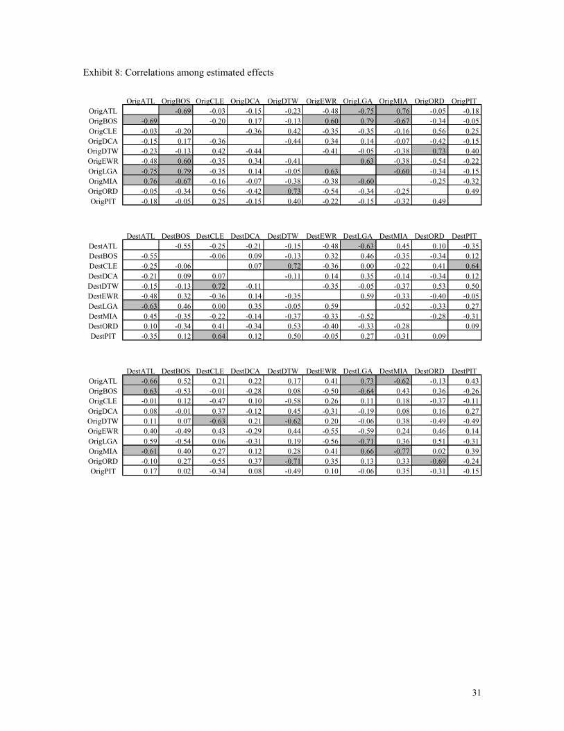
3.5 Correlation among Origin and Destination Effects

The origin and destination effects at each airport turn out not to be independent. In

several instances, there are strong correlations. Exhibit 8 shows rank-order correlations for three

sets of effect estimates: origin with origin, destination with destination, and origin with

destination. We display rank-order (Spearman) correlations in preference to product-moment

(Pearson) correlations because the former are resistant to outliers and mild curvature. Correlations

larger than 0.6 in absolute value are highlighted in Exhibit 8.

Many of the correlations between origin effects are large, especially among airports that

are relatively close geographically. Thus the origin effects of Boston (BOS), LaGuardia (LGA),

and Newark (EWR) tend to be positively correlated. Miami (MIA) and Atlanta (ATL) form a

pair, as do Detroit (DTW) and Chicago (ORD). Perhaps more interesting is that origin effects for

certain airports work in opposite directions. For instance, the southern duo of Atlanta/Miami

correlates negatively with the northeastern trio of Boston/LaGuardia/Newark. Exhibit 9 illustrates

the correlations between origin effects for Boston/LaGuardia and Atlanta/Miami.

Returning to Exhibit 8, analysis of the correlations among destination effects shows

similar behavior, though the overall level of correlation is weaker for destination effects than for

origin effects. Atlanta and Miami again track each other, and both track opposite to

Boston/LaGuardia/Newark. Chicago, Cleveland, Detroit and Pittsburgh form a northwestern

quartet. Exhibit 10 illustrates the correlations between destination effects for Atlanta/LaGuardia

and Cleveland/Detroit.

11

Finally, there are strong correlations between origin and destination effects. Of particular

interest are the correlations on the diagonal in the bottom table of Exhibit 8, which show the

correlations between the origin and destination effects at the same airports. For all ten airports,

these correlations are negative. The correlation is strongest for Miami (-0.77) and LaGuardia (-

0.71) and weakest for Washington (-0.12) and Pittsburgh (-0.15). While this phenomenon might

be interpreted as a result of alternately devoting an airport primarily to serving arrivals or

departures, such regime switches occur over a smaller time scale than we are observing here and

should balance out during an afternoon. Exhibit 11 illustrates the correlations between origin and

destination effects for Miami and LaGuardia.

3.7 Correlations among En Route Effects

It is also possible to study the correlations among en route effects, though there are a

much larger number of correlations in this case. Ten airports generate 100 OD pairs, which

generate 10,000 pairs of OD pairs, e.g., BOS to EWR correlated with LGA to MIA. Even

excluding uninteresting pairs (e.g., PIT to PIT with BOS to BOS) and duplicates (e.g., PIT to

ORD with BOS to ATL, and BOS to ATL with PIT to ORD), we end up with thousands of

meaningful correlations.

Exhibit 12 plots the distribution of the Spearman correlations between pairs of sequences

of en route effects. The distribution is quite symmetric and extends out nearly to ± 0.8. Given that

most correlations are based on 56 daily effect estimates, absolute values above about 0.3 are

statistically significant. Exhibit 13 shows selected instances from the extremes and the middle of

the distribution.

There are a number of OD pairs whose en route effects correlate positively with the en

route effects of other OD pairs. The strongest correlation (0.76) is between flights from Atlanta to

Detroit with flights from Atlanta to Chicago. Since these flights leave from the same origin for

destinations close together, a high positive correlation between en route effects is to be expected.

Many of the OD pairs with positive correlations involve flights that are basically going through

12

the same airspace in the same direction, e.g., Boston/Chicago with LaGuardia/Chicago (0.65) and

Atlanta/Miami with Chicago/Miami (0.65).

The group with correlations near zero are OD pairs whose en route effects do not track

those of any other flights. Many of these flights move, very roughly, at right angles to each other,

such as Pittsburgh/Atlanta versus Newark/Boston. There are, however, exceptions to this rule,

such as the opposite direction pair of LaGuardia/Atlanta and Atlanta/LaGuardia.

The group with negative correlations has daily sequences of en route effects that tend to

move in opposite directions from the effects of other OD pairs. The most prominent examples

involve flights from Atlanta to Chicago, such as Atlanta/Chicago versus Chicago/Miami. One

common thread here is that many of the OD pairs with negative correlations involve flights that

are basically going through the same airspace in opposite directions. Thus, certain routes appear

to be working asymmetrically. This is similar to the phenomenon, noted in Section 3.5 above, of a

given airport s origin effects correlating negatively with its own destination effects. In fact, 81%

of the opposite direction pairs have negative correlation coefficients for their en route effect

estimates.

Our analysis of Exhibit 13 picked up hints that the relative direction of two flights has a

large influence on the correlation of their estimated daily en route effects. To see this directional

effect more directly, we examined a few sets of flights sharing a common origin. Exhibit 14

shows these sets, with a map provided for reference. Consider flights from Miami to Chicago

(MIA_ORD). Flights more or less in the same direction, such as Miami/Atlanta, correlate

positively. As the direction of the second flight moves eastward, the correlation becomes

negative, reaching —0.44 for flights from Miami to Newark or Boston. A similar pattern applies to

Boston/Detroit flights (BOS_DTW). Boston/Chicago flights correlate at 0.55, but changing

direction south leads to negative correlations, reaching —0.57 for Boston/Miami. Similar patterns

apply to the two remaining sets of flights in Exhibit 14.

13

The correlation between en route effects for two flights clearly depends on the relative

directions of flight. In turn, this suggests that the en route effects are measuring the impact of

winds aloft. The positive side of this is that it validates the effects as measures of en route

conditions. The negative side is that winds aloft are outside the control of the FAA, which is more

concerned with en route holding. Presumably, daily variations in winds obscure daily changes in

en route holding.

4. Analysis of Deviations from Estimated Times En Route

We can reduce the influence of winds in our analyses if we shift the data from variations

around long-run averages to deviations from air times filed in flight plans, called Estimated

Times En route (ETEs). Flight plans include sophisticated calculations of the effects of estimated

winds aloft. Deviations from estimated air times thus reflect wind effects only to the extent that

the actual winds encountered differ from those expected before takeoff. Using ETEs also reduces

the effect of nuisance variation caused by differences in aircraft weights or flight paths. To the

extent that filed flight plans are based on accurate forecasts of flight conditions, deviations from

ETEs provide a purer indication of the effects of airspace congestion than do deviations from

long-run average air times. They certainly reflect more closely the element of surprise contained

in variations in air times.

The data for this second analysis came from POET reports for the same 8 airlines and 10

airports over the 62 day period February 28 to April 30, 2001. One day, April 28, had no ETMS

data accessible to POET. We analyzed a total of 24,109 flights. We excluded 4 flights due to

gross errors in the data, 9 flights that had the same origin and destination, and 115 flights from

OD pairs averaging fewer than one flight per day.

Exhibit 15 shows summary statistics for deviations from filed air times by OD pair.

Overall, flights from Cleveland to Detroit were the only ones to average less than their ETEs,

with deviations averaging -2 minutes. The greatest positive deviations were for flights from

14

Pittsburgh to LaGuardia, averaging +15 minutes. The standard deviations typically equaled or

exceeded the mean values, suggesting relatively high variation.

The distributions of the estimated day, destination, and origin effects are shown in

Exhibit 16. Comparing Exhibit 16 to Exhibit 3, we see that this alternative method shows many

estimated effects not centered on zero. We return to Exhibit 16 several times in the discussion

below.

4.1 Day Effects

Exhibit 17 plots the day effects. Because actual flight times averaged about 5 minutes

longer than filed flight times, the estimated day effects were centered around 5 minutes. There

were no outliers or other striking features in the sequence of estimated day effects.

4.2 Origin Effects

It is important to remember that the origin and destination effects sum to zero and

represent variations around the daily average for all flights between all origins and destinations.

Thus, if the day effect is +5, then origin effects represent airport-specific variations above and

below a base level of +5. The origin effects show the positions of the various departure airports

relative to the daily average deviation from flight plans.

Exhibit 16 shows that the estimated origin effects (on the right hand side of the figure)

were less variable than the estimated destination effects (on the left). The origin effects were also

more tightly clustered around zero. This means that the departure airspace created relatively few

deviations from ETEs.

It is noteworthy that the origin with the greatest number of outliers, both positive and

negative, was LaGuardia. While the effects were relatively small, LaGuardia could thus be

regarded as the most inconsistent departure airport. In contrast, both O Hare and Newark showed

remarkable consistency as departure airports and had slightly better than average impacts on

flight times.

15

Exhibit 18 shows estimated origin effects for Atlanta and Miami. The Atlanta sequence

had no outliers. The Miami sequence had low outliers on March 1 and 2, when departing flights

typically had air times about 5 minutes less than the average for those days. In contrast, the

estimates for March 6 and 18 were high outliers. On average, the origin effect for Miami was

about -1 minute, meaning that these flights had about 1 minute less than the daily average

deviation in air time. Since the average day effect was about 5 minutes, this means that flights

leaving Miami experienced about 5-1 = 4 minutes more air time than estimated in their flight

plans.

Comparing Exhibit 18 to Exhibit 5 shows how much different a picture we get when

working with deviations from flight plans instead of variation around long-run averages.

Deviations from flight plans produce fewer outliers, smaller and less variable effect estimates,

and less correlation in daily changes.

4.3 Destination Effects

Destination effects were much more pronounced than arrival effects. Exhibit 16 showed

that the destinations that most consistently added to flight times were Newark, LaGuardia,

Atlanta and Boston. The other six destinations were kinder to expectations, especially Cleveland

and Detroit. The most inconsistent destination airport was either O Hare, if judged by number of

outliers (6 days), or Boston, if judged by interquartile range (6 minutes).

Exhibit 19 plots the estimated destination effects for both Detroit and Boston (compare to

Exhibit 6). Detroit was a good destination, in the sense that its destination effect was almost

always negative. Boston, on the other hand, had seven effect estimates greater than +10 minutes,

including one of about +20 minutes on April 8.

4.4 En Route Effects

En route effects are estimated by the residuals from the linear model. While destination

effects are probably most closely related to traffic management inside the terminal (TRACON)

16

airspace for all arriving aircraft, en route effects are influenced by traffic management initiatives

along specific jet routes.

The estimated en route effects were quite pronounced relative to the origin and

destination effects. Exhibit 20 illustrates this for O Hare airport. The variability in the destination

effects at the far left is matched by the variability of several of the en route effects, such as

Cleveland/Chicago and Miami/Chicago. Furthermore, every one of the distributions of estimated

en route effects involving O Hare had multiple outliers.

Exhibit 21 plots two of the estimated en route effect sequences (compare to Exhibit 7).

The estimated effects for Atlanta/Newark are mostly positive and include +11 minute estimates

on March 2 and 4. In contrast, the estimated effects for Boston/Newark are mostly negative,

which is good, and include one very favorable outlier of —17 minutes on March 4.

4.5 Correlation among Origin and Destination Effects

Unlike the results shown in Exhibit 8, the correlations among estimated effects were

generally weak when based on deviations from ETEs. The universal inverse relationship between

origin and destination effects for the same airport, discussed in section 3.6, was no longer present.

Instead, the same-airport correlations ranged from —0.34 for LaGuardia to +0.45 for Newark.

4.7 Correlations among En Route Effects

Here too the correlations found in section 3 using variations around long-run averages

were much weakened when working with deviations from flight plans. Exhibit 22 shows the

distribution of rank-order correlation coefficients between sets of estimated en route coefficients

(compare to Exhibit 12). Few correlations exceeded 0.3 in absolute value.

5. A NAS Diagnostic Display

The effect estimates described above can be used to attribute variation in air time to one

of four sources: the regional airspace as a whole (day effect), the airspace at the departure airports

(origin effects), the en route airspace (residuals), or the airspace at the arrival airports (destination

17

effects). Large positive values for the estimated effects or residuals point to specific sources of

airborne delays.

This information could be useful to FAA staff at the Air Traffic Control System

Command Center (ATCSCC) in Herndon, VA, which monitors the entire NAS. While the data

used in our method are not available in real time (all the planes have to land first), the analyses

could be helpful in the frequent day after reviews that occupy much of the time of certain staff

at the Command Center and their counterparts among airline operations staff.

The estimates could also be useful for research. For example, one could correlate the

effect estimates with weather conditions or with air traffic control programs. Also, the estimates

could indicate days when there was unusual pressure on particular airports or airspace, flagging

those days for research on how controllers respond to these conditions.

To formally process timeplots of effects, one could apply the well-established methods of

statistical process control (SPC). SPC is concerned with detecting departures from a consistent

level of background randomness, i.e., detecting when a process is out of control, and is in

widespread use in the manufacturing sector. In particular, the individuals chart (Montgomery and

Runger 1994) can be used to detect deviations from purely random variation, including drift in

the mean level and outliers. (The same methods could also be applied directly to airtimes for OD

pairs, but this would not exploit the diagnostic value of plots of estimated effects.) Exhibit 23

illustrates the use of individuals charts applied to estimated effects. In the upper part of the

exhibit, the destination effects for Chicago are shown to be out of control on three days. In the

lower part of Exhibit 23, the individuals chart identifies two outliers among the sequence of

destination effects for Newark. The main advantage of using formal charting methods from SPC

is to remove the subjective element from interpretation of the timeplots of estimated effects.

Subjectivity would not be an issue with the EWR data in Exhibit 23, but could be with the ORD

data.

18

It would be helpful to those concerned with air traffic flow to display the estimated

effects graphically on a map. How to design such a display for maximum impact is beyond the

scope of this paper, but we can suggest a scheme to make the point. If there were large positive en

route effect estimates for flights between two airports, a red line might connect the two. If many

red lines flow through the airspace of one of the twenty regional Air Route Traffic Control

Centers (ARTCCs) responsible for continental US airspace, that ARTCC would be singled out for

further examination. A circle divided at its equator might represent each major airport on the

map. If the departure airspace were estimated to be causing delays, the bottom half of the circle

representing that airport could be displayed red. Problems with the arrival airspace could cause

the top half of the circle to be red. Unusually good conditions could be indicated using the color

green. Conditions in no way unusual would not be shown, in order to simplify the display.

6. Methodological Challenges

In developing the methodology, our strategy has been to err on the side of simplicity and

transparency. However, we should acknowledge that certain technical challenges remain.

One issue is the estimation of uncertainty. The presentation above reported point

estimates without standard errors or confidence intervals. Statistical inference in this

methodology is complicated by several factors. While the use of individuals charts to monitor

timeplots for out of control conditions is a one answer to the problem of inference, the effect

estimates do not strictly satisfy the assumption of individual charts that all points have the same

variability. When computing variations around long-run averages, there is sampling variability in

the long-run average point-to-point air times that serve as the baseline. Also, the daily average

deviations are based on numbers of flights that vary from day to day. Furthermore, there is a

positive association between the means and standard deviations of air times. One could respond

to these problems by expressing deviations in percentage rather than absolute terms, or by

working with standardized (i.e., zero mean, unit variance) deviations in air times. Either response

would alleviate the statistical problem but complicate interpretation of the results.

19

A second issue is the nonlinear, iterative nature of the calculations of effect estimates.

Even if we could correctly summarize the variability of the input data in the tables of deviations,

the use of a nonlinear solver greatly complicates analysis of how that variability gets transmitted

to the effect estimates. Bootstrapping methods (Efron and Tibshirani 1993) may the useful here,

although they would be very computationally expensive, especially if the resampling unit were a

single flight. More practical might be jackknife estimates of standard error (Mosteller and Tukey

1977, Efron and Tibshirani 1993), deleting whole cells to generate the variability estimates.

A third issue is that the solutions to the nonlinear programming problem are not

necessarily the most parsimonious estimates. For instance, if a deviations table were to have the

same constant value in every cell, the effect estimates should, but would not, be limited to a

single nonzero day effect, with all origin and destination effects equal to zero. Likewise, a table

developed from one nonzero origin effect and one nonzero destination effect would be fit using

nonzero values for all possible effects. Although the fits produced by the nonlinear program are

as accurate as the ideal fits, they are nowhere near as simple. This defect might be remedied by

introducing degree of freedom penalties into the objective function. Since this part of the model is

already obscure for most FAA and airline personnel, additional complication here would be

tolerable.

A fourth issue is the possibility that different airlines create their flight plans differently,

planning longer or shorter air times for the same OD pair. This could confound the interpretation

of results, to the extent that different airlines dominate different airports. Similarly, if one airline

were to drop or add service at an airport, and also thereby change the mix of aircraft using that

airport, the method might detect a change in the airport s origin effect. This would be problematic

for the FAA since it is a change outside the purview of the agency, thereby rendering the change

as noise instead of signal. The impact of these sorts of policy-irrelevant background changes can

be reduced by working with a moving window of the most recent data.

20

A separate analysis showed that it is sometimes true that different airlines develop

different ETEs for the same OD pairs. To investigate this potential problem, we analyzed ETEs

for flights made by American, Delta, and United Airlines to and from Atlanta, Boston, Dallas and

Chicago during the period March 19 to May 14, 2001. These were again ETMS data extracted by

POET. Flights from Dallas to Atlanta had an average ETE of 82 minutes for Delta Airlines, 83

minutes for United Airlines, and 88 minutes for American Airlines. The difference between the

ETEs for American and Delta was 6.4 minutes, with a standard error of 0.4 minute. This

difference is both statistically and substantively significant. Fortunately, the analysis also showed

that more often than not, the airlines ETEs were quite similar.

A fifth issue is the possibility that airline dispatchers preempt the calculation of

congestion. The analysis based on deviations from long-run averages suffers from the problem of

being strongly influenced by winds. The corresponding potential problem with the analysis based

on deviations from flight plans is that airline dispatchers might anticipate congestion and pad the

filed flight times. This adjustment would weaken the ability of the row+column analysis to detect

the congestion.

There were pronounced variations in filed flight times over the approximately two month

period of the special study of ETEs. We can think of these data in the familiar row+column

framework, attributing variations in ETEs to a linear combination of daily effects that applied to

all hours of arrival and hourly effects that applied to all days. The daily variations might be

interpreted as adjustments for seasonal changes in the jet stream. These policy-irrelevant

variations are more or less neutralized in the analysis based on ETEs. The hourly variations might

be interpreted as adjustments made by airline dispatchers in anticipation of delays. These

variations undermine the ability of the analysis based on ETEs to detect airborne delays.

Luckily, for most of the OD pairs, variations from day to day were much larger than

variations from hour to hour. Exhibit 24 shows results from a two-way analysis of variance

without interactions, using ETE as the response and day and arrival hour as factors. In all twelve

21

cases, the mean square for residuals was relatively small compared to the other two sources of

variation. This means that the linear additive model was accurate, and little was lost by not

considering a model with interaction terms. In eleven of the twelve cases, the mean square for the

day effect was substantially larger than the mean square for the arrival hour effect, suggesting that

any possible schedule manipulation to anticipate congestion was a relatively minor effect. (The

single exception was for flights from DFW to ATL.)

The fact that the mean square for arrival hour was much smaller than that for day does

not mean that the hour effect was not statistically significant. In fact, both effects were highly

significant for every OD pair studied. However, the magnitude of the effect was usually small

enough that the analysis based on ETEs could still be useful. Exhibit 25 shows mean ETEs for the

cases most favorable (BOS to ATL) and least favorable (DFW to ATL) to our method.

7. Summary and Conclusions

Expeditious movement of air traffic is made easier when flight times are consistent.

However, using ETMS data, we have documented significant variations in air times. We

developed a method to identify and estimate sources of variation throughout a regional airspace.

One variant of the method normalizes each day s average airtime for each OD pair by subtracting

the long-term average air time for that pair. The other variant subtracts the estimated time en

route (ETE) filed in the flight plan. The method uses an outlier-resistant version of row+column

analysis to estimate effects attributed to the date, the origin airport, the en route airspace, and the

destination airport.

The resulting sequences of estimated effects can themselves be studied as a dataset. One

use is to identify unusually bad or good days within the region. Another is to pinpoint the sources

of airborne delays for further analysis. The estimated effects can also be correlated with each

other, revealing subsets of airports that track each other s problems, subsets that work in opposite

ways, and the tradeoff between arrival and departure operations within individual airports.

22

This methodology could readily be scaled up to handle OD pairs spanning the entire

NAS. The results could be presented graphically to give a useful summary of airborne delay

issues for post-operational analysis. And the method should be applicable to analysis of measures

other than air time, such as total gate-to-gate times, i.e., from departure gate to arrival gate. Work

along these lines would maximize return on the large public investment in air traffic data.

23

Acknowledgements

Useful comments were provided by Mike Ball, Steve Bradford, Dan Citrenbaum, Bob

Hoffman, Dave Knorr, Ed Meyer, Tim Niznik, Joe Post and George Solomon.

References

Efron, B.; Tibshirani, R. 1993. An Introduction to the Bootstrap. New York: Chapman & Hall.

Emerson, J. and D. Hoaglin. 1983. Analysis of Two-Way Tables by Medians. In D. Hoaglin, F

Mosteller, and J. Tukey, eds., Understanding Robust and Exploratory Data Analysis. New York,

NY: Wiley.

ETMS, Enhanced Traffic Management System. 2001.

http://www.atcscc.faa.gov/Information/ETMS/etms.html

Montgomery, D. and G. Runger. 1994. Applied Statistics and Probability for Engineers. New

York, NY: Wiley.

Mosteller F. and Tukey, J. 1977. Data Analysis and Regression: A Second Course in Statistics.

Reading, MA: Addison-Wesley.

POET, Post-Operations Evaluation Tool. 2001. http://www.amtsys.com/poet/home.htm

24

Exhibit 1: Illustrating the calculation of origin, destination, and en route effects for a specific day

Origin\Destination A B C DA 65 80 100B 75 100 120C 90 100 135D 100 110 125

Average Air Times for Day 7

Origin\Destination A B C DA 56 81 107B 69 124 132C 94 106 157D 109 121 146

Deviations from Overall Averages for Day 7

Origin\Destination A B C DA -9 1 7B -6 24 12C 4 6 22D 9 11 21

Analysis of Deviations for Day 7

En Route Effects A B C D Origin Effects:A 0.0 0.0 0.0 -10.0B 0.0 18.0 0.0 -5.0C 0.0 0.0 0.0 5.0D 0.0 0.0 0.0 10.0

Destination Effects: -8.0 -6.0 4.0 10.0 7.0 = Day Effect

25

Exhibit 2: Summary statistics for air times (in minutes) for OD pairs

Counts DestinationATL BOS CLE DCA DTW EWR LGA MIA ORD PIT

ATL 266 97 387 256 415 376 310 522 134BOS 230 84 563 96 219 645 107 424 159CLE 194 71 90 108 139 118 169DCA 346 564 81 163 138 612 200 423 105

Origin DTW 283 86 101 185 273 152 55 386 47EWR 372 273 169 194 248 177 540 149LGA 363 666 80 603 192 128 508 165MIA 323 146 55 203 86 177 193 292 117ORD 545 445 143 443 398 510 495 248 174PIT 229 150 122 94 118 200 46 241

Averages DestinationATL BOS CLE DCA DTW EWR LGA MIA ORD PIT

ATL 122 78 76 88 105 99 85 95 74BOS 150 98 79 107 56 47 184 141 85CLE 89 84 51 25 66 71 63DCA 93 65 59 73 43 41 136 107 40


Std Dev’s DestinationATL BOS CLE DCA DTW EWR LGA MIA ORD PIT

ATL 9 5 11 6 10 9 6 7 6BOS 11 7 6 8 10 7 14 12 6CLE 9 13 4 2 11 7 7 8DCA 9 7 6 5 8 5 11 9 3


26

Exhibit 3: Distributions of estimated effects

-20

0

20

40

Day

DestATL

DestBOS

DestCLE

DestDCA

DestDTW

DestEWR

DestLGA

DestMIA

DestORD

DestPIT

OrigATL

OrigBOS

OrigCLE

OrigDCA

OrigDTW

OrigEWR

OrigLGA

OrigMIA

OrigORD

OrigPIT

27

Exhibit 4: Estimated day effects

Day

-5

0

5

10

28-Jan 4-Feb 11-Feb 18-Feb 25-Feb 4-Mar 11-Mar 18-Mar 25-Mar

28

Exhibit 5: Selected estimated origin effects

OrigATL

-10

-5

0

5

10


OrigMIA

-15

-10

-5

0

5

10

15

20

25


29

Exhibit 6: Selected estimated destination effects

DestDTW

-10

-5

0

5

10


DestBOS

-10

-5

0

5

10

15

20


30

Exhibit 7: Selected estimated en route effects

ATL:EWR

-10

-5

0

5

10

15


BOS:EWR

-20

-15

-10

-5

0

5

10

15

20


31

Exhibit 8: Correlations among estimated effects

OrigATL OrigBOS OrigCLE OrigDCA OrigDTW OrigEWR OrigLGA OrigMIA OrigORD OrigPITOrigATL -0.69 -0.03 -0.15 -0.23 -0.48 -0.75 0.76 -0.05 -0.18OrigBOS -0.69 -0.20 0.17 -0.13 0.60 0.79 -0.67 -0.34 -0.05OrigCLE -0.03 -0.20 -0.36 0.42 -0.35 -0.35 -0.16 0.56 0.25OrigDCA -0.15 0.17 -0.36 -0.44 0.34 0.14 -0.07 -0.42 -0.15OrigDTW -0.23 -0.13 0.42 -0.44 -0.41 -0.05 -0.38 0.73 0.40OrigEWR -0.48 0.60 -0.35 0.34 -0.41 0.63 -0.38 -0.54 -0.22OrigLGA -0.75 0.79 -0.35 0.14 -0.05 0.63 -0.60 -0.34 -0.15OrigMIA 0.76 -0.67 -0.16 -0.07 -0.38 -0.38 -0.60 -0.25 -0.32OrigORD -0.05 -0.34 0.56 -0.42 0.73 -0.54 -0.34 -0.25 0.49OrigPIT -0.18 -0.05 0.25 -0.15 0.40 -0.22 -0.15 -0.32 0.49

DestATL DestBOS DestCLE DestDCA DestDTW DestEWR DestLGA DestMIA DestORD DestPITDestATL -0.55 -0.25 -0.21 -0.15 -0.48 -0.63 0.45 0.10 -0.35DestBOS -0.55 -0.06 0.09 -0.13 0.32 0.46 -0.35 -0.34 0.12DestCLE -0.25 -0.06 0.07 0.72 -0.36 0.00 -0.22 0.41 0.64DestDCA -0.21 0.09 0.07 -0.11 0.14 0.35 -0.14 -0.34 0.12DestDTW -0.15 -0.13 0.72 -0.11 -0.35 -0.05 -0.37 0.53 0.50DestEWR -0.48 0.32 -0.36 0.14 -0.35 0.59 -0.33 -0.40 -0.05DestLGA -0.63 0.46 0.00 0.35 -0.05 0.59 -0.52 -0.33 0.27DestMIA 0.45 -0.35 -0.22 -0.14 -0.37 -0.33 -0.52 -0.28 -0.31DestORD 0.10 -0.34 0.41 -0.34 0.53 -0.40 -0.33 -0.28 0.09DestPIT -0.35 0.12 0.64 0.12 0.50 -0.05 0.27 -0.31 0.09

DestATL DestBOS DestCLE DestDCA DestDTW DestEWR DestLGA DestMIA DestORD DestPITOrigATL -0.66 0.52 0.21 0.22 0.17 0.41 0.73 -0.62 -0.13 0.43OrigBOS 0.63 -0.53 -0.01 -0.28 0.08 -0.50 -0.64 0.43 0.36 -0.26OrigCLE -0.01 0.12 -0.47 0.10 -0.58 0.26 0.11 0.18 -0.37 -0.11OrigDCA 0.08 -0.01 0.37 -0.12 0.45 -0.31 -0.19 0.08 0.16 0.27OrigDTW 0.11 0.07 -0.63 0.21 -0.62 0.20 -0.06 0.38 -0.49 -0.49OrigEWR 0.40 -0.49 0.43 -0.29 0.44 -0.55 -0.59 0.24 0.46 0.14OrigLGA 0.59 -0.54 0.06 -0.31 0.19 -0.56 -0.71 0.36 0.51 -0.31OrigMIA -0.61 0.40 0.27 0.12 0.28 0.41 0.66 -0.77 0.02 0.39OrigORD -0.10 0.27 -0.55 0.37 -0.71 0.35 0.13 0.33 -0.69 -0.24OrigPIT 0.17 0.02 -0.34 0.08 -0.49 0.10 -0.06 0.35 -0.31 -0.15

32

Exhibit 9: Selected correlations among origin effects

-15

-10

-5

0

5

10

-15 -10 -5 0 5 10

OrigBOS

Ori

gL

GA

-15

-10

-5

0

5

10

15

20

25

-10 -5 0 5 10

OrigATL

Ori

gM

IA

33

Exhibit 10: Selected correlations among destination effects

-6

-4

-2

0

2

4

6

8

10

12

14

-20 -15 -10 -5 0 5 10 15 20

DestATL

DestL

GA

-10

-8

-6

-4

-2

0

2

4

6

-10 -5 0 5 10 15

DestCLE

DestD

TW

34

Exhibit 11: Selected correlations among origin and destination effects for the same airport

-15

-10

-5

0

5

10

15

20

25

-15 -10 -5 0 5 10 15 20 25

OrigMIA

DestM

IA

-6

-4

-2

0

2

4

6

8

10

12

14

-15 -10 -5 0 5 10

OrigLGA

DestL

GA

35

Exhibit 12: Distribution of Spearman correlations between sets of en route effects

0%

5%

10%

-1.0 -0.5 0.0 0.5 1.0

Spearman Correlation

36

Exhibit 13: Correlations between en route effects for selected OD pairs

1st Route 2nd Route Correlation

ATL_DTW ATL_ORD 0.76LGA_DTW EWR_ORD 0.74ATL_ORD MIA_ORD 0.68LGA_DTW LGA_ORD 0.68ORD_ATL ORD_MIA 0.68ATL_DCA MIA_DCA 0.66

EWR_ORD LGA_ORD 0.66EWR_ORD ORD_ATL 0.66ATL_MIA ORD_MIA 0.65

BOS_ORD LGA_ORD 0.65

ATL_BOS EWR_PIT 0.00BOS_DCA CLE_ORD 0.00CLE_ATL MIA_DTW 0.00DCA_BOS BOS_PIT 0.00DTW_ATL MIA_LGA 0.00EWR_ATL CLE_DCA 0.00LGA_ATL ATL_LGA 0.00MIA_ATL DCA_BOS 0.00ORD_ATL CLE_ORD 0.00PIT_ATL EWR_BOS 0.00

BOS_ORD ATL_ORD -0.63BOS_ORD BOS_MIA -0.63MIA_ORD BOS_ORD -0.64MIA_ORD EWR_ORD -0.64ATL_ORD ATL_MIA -0.65LGA_DTW ATL_DTW -0.67LGA_DTW ATL_ORD -0.70ORD_ATL ATL_ORD -0.73

EWR_ORD ATL_ORD -0.77ORD_MIA ATL_ORD -0.78

37

Exhibit 14: Illustrating the influence of direction of flight on en route correlations

1st Route 2nd Route Correlation

MIA_ORD MIA_ATL 0.39MIA_ORD MIA_CLE 0.34MIA_ORD MIA_DTW 0.04MIA_ORD MIA_PIT -0.13MIA_ORD MIA_LGA -0.23MIA_ORD MIA_DCA -0.35MIA_ORD MIA_BOS -0.44MIA_ORD MIA_EWR -0.44

BOS_DTW BOS_ORD 0.55BOS_DTW BOS_CLE 0.25BOS_DTW BOS_PIT 0.09BOS_DTW BOS_EWR -0.13BOS_DTW BOS_LGA -0.23BOS_DTW BOS_ATL -0.39BOS_DTW BOS_DCA -0.41BOS_DTW BOS_MIA -0.57

ORD_EWR ORD_DTW 0.25ORD_EWR ORD_BOS 0.15ORD_EWR ORD_DCA -0.01ORD_EWR ORD_PIT -0.11ORD_EWR ORD_CLE -0.14ORD_EWR ORD_LGA -0.18ORD_EWR ORD_ATL -0.45ORD_EWR ORD_MIA -0.56

ATL_BOS ATL_MIA 0.59ATL_BOS ATL_DCA 0.39ATL_BOS ATL_LGA 0.21ATL_BOS ATL_EWR 0.04ATL_BOS ATL_CLE -0.35ATL_BOS ATL_DTW -0.39ATL_BOS ATL_ORD -0.48ATL_BOS ATL_PIT -0.53

38

Exhibit 15: Summary statistics for deviations from filed air times by OD pair

CountsDestination

ATL BOS CLE DCA DTW EWR LGA MIA ORD PIT ATL 303 160 433 305 485 435 355 594 167 BOS 263 92 621 127 263 724 115 476 189 CLE 190 88 104 120 154 133 187

Origin DCA 391 636 98 183 153 706 229 495 119 DTW 312 110 90 204 280 168 411 78 EWR 467 303 162 220 270 181 569 160 LGA 409 734 103 687 201 154 582 189 MIA 363 177 261 106 194 219 313 107 ORD 613 508 167 530 426 581 570 273 216 PIT 268 191 153 86 155 224 271

AveragesDestination

ATL BOS CLE DCA DTW EWR LGA MIA ORD PIT ATL 6 0 6 2 10 4 3 4 4 BOS 9 2 2 3 8 9 4 5 4 CLE 7 10 2 -2 11 11 6 DCA 9 11 3 1 6 7 2 3 0

Origin DTW 8 9 0 2 10 11 4 2 EWR 7 6 2 1 2 3 5 4 LGA 8 6 1 6 1 3 5 0 MIA 7 6 5 2 7 0 4 4 ORD 7 5 2 2 0 9 8 3 3 PIT 9 11 2 1 13 15 4

Std Dev’sDestination

ATL BOS CLE DCA DTW EWR LGA MIA ORD PIT ATL 8 6 5 4 9 6 4 8 4 BOS 8 6 4 5 7 6 7 8 6 CLE 8 12 3 2 7 7 9 DCA 8 9 6 5 7 7 7 8 4

Origin DTW 8 5 2 3 6 5 7 2 EWR 8 7 8 3 5 6 11 12 LGA 11 9 4 4 4 6 10 4 MIA 8 9 6 5 10 8 9 4 ORD 7 10 3 5 5 9 7 7 4 PIT 7 11 3 4 6 7 6

39

Exhibit 16: Distributions of effects estimated from flight plans

-10

0

10

20

30

40

Day

DestATL

DestBOS

DestCLE

DestDCA

DestDTW

DestEWR

DestLGA

DestMIA

DestORD

DestPIT

OrigATL

OrigBOS

OrigCLE

OrigDCA

OrigDTW

OrigEWR

OrigLGA

OrigMIA

OrigORD

OrigPIT

40

Exhibit 17: Day effects estimated from flight plans

Day

0

5

10

27-Feb 6-Mar 13-Mar 20-Mar 27-Mar 3-Apr 10-A pr 17-A pr 24-Apr 1-May

41

Exhibit 18: Selected origin effects estimated from flight plans

OrigA TL

-5

0

5

27-Feb 6-Mar 13-Mar 20-Mar 27-Mar 3-Apr 10-A pr 17-A pr 24-Apr 1-May

OrigMIA

-10

-5

0

5

27-Feb 6-Mar 13-Mar 20-Mar 27-Mar 3-Apr 10-Apr 17-Apr 24-Apr 1-May

42

Exhibit 19: Selected destination effects estimated from flight plans

DestDTW

-10

-5

0

5


DestBOS

-5

0

5

10

15

20

25


43

Exhibit 20: Comparison of distributions of all effects related to ORD

-15

-10

-5

0

5

10

15

20

25

DestORD

OrigORD

ATL_ORD

BOS_ORD

CLE_ORD

DCA_ORD

DTW_ORD

EWR_ORD

LGA_ORD

MIA_ORD

ORD_BOS

ORD_CLE

ORD_DCA

ORD_DTW

ORD_EWR

ORD_LGA

ORD_MIA

ORD_ORD

ORD_PIT

PIT_ORD

44

Exhibit 21: Selected en route effects estimated from flight plans

ATL:EWR

-10

-5

0

5

10

15


BOS:EWR

-20

-15

-10

-5

0

5

10


45

Exhibit 22: Distribution of en route Spearman correlations using flight plans

0%

5%

10%

15%

20%

-1 -0.5 0 0.5 1

Spearman Correlation

46

Exhibit 23: Individuals charts for selected origin effects estimated from flight plans

6050403020100

20

10

0

-10

Observation Number

Indiv

idu

al V

alue

I Chart for DestORD

11

1

X=-0.3593

3.0SL=12.44

-3.0SL=-13.16

6050403020100

35

30

25

20

15

10

5

0

-5

-10

Observation Number

Indiv

idua

l Valu

e

I Chart for DestEWR

1

1

X=4.719

3.0SL=14.45

-3.0SL=-5.009

47

Exhibit 24: Sources of variation in filed air times (ETEs)

Mean SquareOrigin Destination Day Arrival Hour ResidualATL BOS 331 81 8

DFW 503 215 19ORD 393 98 13

BOS ATL 449 16 8DFW 970 170 55ORD 876 290 38

DFW ATL 258 478 14BOS 750 350 46ORD 688 139 42

ORD ATL 309 156 19BOS 369 68 13DFW 1175 143 27

48

Exhibit 25: Most favorable and least favorable cases for use of deviations from ETEs

BOS to ATL:

DFW to ATL:

110

125

140

155

170

12345678910111213141516171819202122232425262728293031323334353637383940414243444546474849505152535455565758

Means of ETE

Day

ETE

110

125

140

155

170

01002003004005001000120013001400150016001700180019002000210022002300

Means of ETE

Arrival_Hour

ETE

70

85

100

115

130

12345678910111213141516171819202122232425262728293031323334353637383940414243444546474849505152535455565758

Means of ETE

Day

ETE

70

85

100

115

130

01002003004005006007001100120013001400150016001700180019002000210022002300

Means of ETE

Arrival_Hour

ETE

estimating components of variation in flight times

Documents