Estimating Beta-Coefficients of German Stock Data: ANon-Parametric Approach

Maik Eisenbeiß (maik.eisenbeiss@uni-muenster.de)Westfalische Wilhelms-Universitat Munster

Goran Kauermann (gkauermann@wiwi.uni-bielefeld.de)Universitat Bielefeld

Willi Semmler (semmlerw@newschool.edu)Universitat Bielefeld and New School University New York

Abstract. Although the consumption based asset pricing theory appears to be theoreti-

cally superior and more elegant than the beta pricing model, yet in practice the beta pric-

ing model is more widely applied. Indeed, beta pricing models are one of the most widely

adopted tools in financial analysis. They easily allow to handle systematic risk as priced in

financial assets. However, accurately estimating beta-coefficients is not as straightforward

as implicitly suggested by Sharpe’s standard market model, i.e., simply using the ordinary

least-squares (OLS) regression. This is primarily because beta-coefficients cannot gener-

ally be assumed as being stable over time. In order to overcome this deficiency, we present

and apply a non-parametric estimation technique that allows capturing this time effect

and promises both, more reliable estimates than obtained with an OLS-regression as well

as a better manageability compared to the existing econometric approaches dealing with

time-varying beta-coefficients. Estimation results for constant and time varying betas are

presented for portfolios of German industries.

Keywords: systematic risk, time-varying beta-coefficients, non-parametric estimation,

varying-coefficient model

1 Introduction

In the financial literature there are two paradigms used for studying assetpricing and portfolio decisions. The first paradigm is static and is basedon the traditional capital asset pricing model (CAPM) of Markowitz (1952)and Sharpe (1964), whereas the second approach is based on intertempo-ral decisions of economic agents who exhibit well specified preferences forconsumption over time. The latter approach is called consumption basedasset pricing which is well grounded in economic theory. It answers mostasset pricing and portfolio decisions in principle, yet it does not work wellin practice. The latter attempts to tie the stochastic discount factor, crucialfor pricing assets, to preferences and consumption data, but its performancein practice is rather limited.1

On the other hand, models that use factors for asset pricing are easyto handle in practice since they are usually obtained in linear form throughlinear regressions. The typical example for this is the CAPM where a beta,as a price for risk, prices the asset and justifies the return from an assetor portfolio of assets. The CAPM also allows to obtain a discount factorin linear form from the beta estimations2. If the presumed consumptionbased asset pricing model is of special form, for example representing specialpreferences then the CAPM represents an equivalent form of asset pricing3.

Apart from the ongoing research on the theoretical relationship of theCAPM to the consumption based asset pricing model, in practice beta esti-mates have always been used as a measure of risk in modern finance. Theyhave contributed to a variety of applications such as testing of asset pric-ing theories, estimating cost of capital, hedging market exposure as well asportfolio performance evaluation and thus they are one of the most widelyadopted instruments among practitioners and financial economists in orderto measure and manage risk. Wells (1995, p. 5) nicely summarizes thesignificance of beta in just one sentence: “It is one of the few regressioncoefficients, simple or otherwise, that people actually pay money to get.”As a consequence, accuracy in the measurement of the beta-coefficient canbe considered a striking topic.

1For an extensive evaluation of those two theories, see Cochrane (2001, ch. 9) andCampbell and Cochrane (2000).

2See Cochrane (2001, chs. 6 and 9).3See Cochrane (2001, ch. 9).

1

During the last three decades numerous studies have addressed the ques-tion of beta’s stability over time. Among the most prominent studies areBlume (1971), Baesel (1971), Altman, Jacquillat, and Levasseur (1974),Roenfeldt, Griepentrong, and Pflaum (1978), Alexander and Chervany (1980)and Theobald (1981). What they share in common is the observation thatbeta-coefficients are far from being stable. Despite this general consensus,still the most widely adopted approach for estimating beta is the ordinaryleast-squares regression. In its simplest form it is often based on the follow-ing model framework, known as the market model :

Rj = αj + βjRM + εj (1)

with Rj and RM denoting the holding period excess return on the jth secu-rity and on the overall market M , respectively4. The parameter αj depictsthe security’s expected return if the market is neutral, i.e., if RM = 0, andεj quantifies changes in the holding period excess return due to changes thatare exclusively firm-specific. The beta-coefficient is, of course, depicted byβj and assesses the impact of movements in the market on the jth security.However, such an approach assumes constant coefficients and in the con-text of time-varying betas it is likely to produce inconsistent results. Onereason for its prevailing use might be due to the fact that its usage is rela-tively straightforward and that the existing econometric alternatives, whichpromise more accurate estimates, are much harder to pursue. Among thoseeconometric alternatives the most widely adopted approach is to estimatebeta as a time-series process using the Kalman filter. In this respect, thetime-path of beta is commonly modelled as a process which relates today’sbeta value either to its overall mean or to last periods’ beta values5.

The remainder of this paper concentrates on a fundamentally differentapproach: Using a non-parametric estimation technique, we treat the beta-coefficient as an unspecified function of time. The estimation results whichare based on daily data of industry replicating portfolios for the Germanstock market between 1992 and 2003 support our approach as a useful andespecially easy accessible compromise in the environment of estimating time-varying beta-coefficients. Moreover, the results do not only confirm the

4The holding period excess return depicts the holding period return in excess of therisk-free rate rf .

5See Schaefer, Brealey, Hodges, and Thomas (1975)

2

general hypothesis of non-constant betas but they also suggest a counter-cyclical behavior of several industry groups’ beta-coefficients with respectto the state of the market. On average, betas tend to be significantly largerin bear-markets than in bull-markets for these industry groups. Hence,market phases can be considered a driving force for the variability of beta-coefficients.

The paper is structured as follows: Chapter 2 introduces the non-parametricapproach for estimating time-varying beta-coefficients. Chapter 3 then pro-vides a overview of the data before discussing the main results. Chapter 4finally draws the main conclusions.

2 A Non-Parametric Estimation Approach

Essentially, the starting point of the non-parametric estimation approach isto generalize the market model (1) by including a component which accountsfor the time-variation in the beta-coefficient. The “generalized” marketmodel is given by

Rjt = αj + βjRMt + βj(t)RMt + εjt (2)

with βj(t) capturing the time-effect embedded in the systematic risk com-ponent of the jth security. Apparently, coefficients βj and βj(t) in (2) arenot identifiable unless we impose

∫βj(t)dt = 0. In this respect, the para-

metric beta-estimate can be regarded as the mean value of beta for thewhole period under consideration. Thus, dependent on the time-period itis additively increased or decreased by the estimate of its non-parametriccounterpart. In other words, the estimated beta-coefficient in period k isgiven by βk = β + ˆ

β(k).In the context of the non-parametric estimation literature, a model of this

form is known as a varying-coefficient model6. The main idea of a varying-coefficient model is to provide a framework in which the influence of thepredictor variables on the response variable is linear while the correspondingcoefficients are no longer treated as constants but rather as functions ofother variables. In particular, βj(t) expresses the multiplicative interactionor temporal changes, respectively, of the influence of RMt.

6The varying-coefficient model was first proposed by Hastie and Tibshirani (1993).

3

A varying-coefficient model as in (2) can be fitted to data by finding thesolution of the following penalized least-squares criterion7

minαj ,βj

T∑

t=1

(Rjt − αj − βjRMt − βj(t)RMt

)2

+ λj

∫ b

aβ′′j (t)2dt. (3)

While the first term measures the goodness of fit, the second term penalizesthe curvature of the function βj(.). The so-called smoothing parameter λj

deserves special attention, since it controls the trade-off between bias andvariance of the fit. For λ → 0 the influence of the penalty term disappearsand the resulting function tends to interpolate between the observations.In contrast, λ → ∞ forces the penalty term to dominate and thus yields asimple linear regression fit. In this respect, Wood (2000) has proposed analgorithm which “automatically” determines an “optimal” level of smooth-ing. This algorithm is provided as the function gam() in the package mgcv

of the (public domain) statistical software environment R. The appropriateR-commands can be found in Appendix A.

In (2) we have not said much about the structure of the residuals εjt.The natural assumption of homoscedasticity is likely to be too simplisticand two potential violations spring in our mind: First, residuals can becorrelated and secondly, the residual variance can change over time. In thefirst case, the automatic smoothing parameter selection method by Wood(2000) would fail in the presence of autocorrelated errors. In such a case,the smoothing parameter should be determined by hand or by other moreelaborated methods suggested in the paper by Opsomer, Wang, and Yang(2001). In the data example at hand autocorrelation was not observable,based on both, a graphical investigation and the Durbin Watson statistics.

In contrast, we found clear indication of heteroscedasticity in the dataafter investigation of the fitted residuals based on a first smooth estimate.Note that homoscedasticity is an integral assumption in the estimation stepas well as when drawing inference from the estimation results. Hence, inthe case of heteroscedastic residuals the estimation approach as describedabove does not necessarily guarantee reliable or at least efficient estimates.We cope with heteroscedastic residuals by pursuing a two-step estimationapproach: The first step is to determine the squared residuals from the

7A technical introduction into a fitting mechanism of this kind for a varying-coefficientmodel can be found in Appendix C.

4

estimation results of model (2) by assuming (working) homoscedasticity.This yields working residuals defined through

εjt = (Rjt − Rjt)2. (4)

A simple exploratory investigation is available by plotting ε2jt against t.

Heteroscedasticity is now visualized by the structure in the plot. In a non-parametric and flexible way we can model dependence of residual variationon time with a generalized additive gamma model. This is accommodatedby modelling the squared residuals as

µ2jt = V ar(ε2

jt) = E(ε2jt) = g{αj + fj(t)} (5)

where fj(.) is a smooth but otherwise unspecified non-parametric functionand g(.) is called the inverse link function. Based on a gamma model wechoose g−1(µ) = −1/µ.8 The major idea behind the gamma model is, thatthe variance of ε2

jt is proportional to µ4jt and with fj(t) = constant = 0 a

homoscedastic (normal residual) model results. Hence, fj(t) captures theheteroscedasticity over time. Model (5) falls also in the class of modelswhich can be fitted with the gam(.) procedure in R as demonstrated in theappendix. In particular, model (5) can be regarded as a special case of thefamily of generalized additive models, which themselves are a generalizationof additive regression models9. The scedasticity-structure estimated by thegamma-model can now be used to refit model (2) in a weighted mannerwhich implicitly accounts for heteroscedasticity. Let therefore ωjt = 1/µ2

jt

be weights constructed from the fitted model (5). These weights are nowused to fit model (2) in a weighted form. In practice, this can be pursuedby inserting weights in the fitting routine, as it is implemented in the so farused R software. More details are found in Appendix A.

8See McCullagh and Nelder (1989).9See Hastie and Tibshirani (1990). While additive models linearly associate the re-

sponse variable with an additive sum of (non-parametric) functions of the predictor vari-ables, generalized additive models allow the response variable to depend on the additivepredictor through a nonlinear relationship.

5

3 Data and Results

3.1 The Data

In this section we want to demonstrate the potentials of the non-parametricestimation approach by applying the model to a variety of industry groupsbased on data from the German stock market.

The data used are daily observations from April 1991 to March 2003. Inits original form, it comprises stock prices for a range of selected companieswith listed securities at the German stock market as well as observationson the CDAX performance index. The data are from the Reuters 3000 Xtra

database. Concerning the risk-free rate in the market model we use overnightmoney market rates obtained from the German Bundesbank10.

The following seven industry groups will be regarded in the analysis11:Automobile, Banks, Consumer, Industrial, Retail, Pharma & Healthcareand Utilities. The most obvious and, of course, the most accurate way torefer to these industry groups would be to consider several industry-specificstock market indexes. However, due to lacking data, the approach pur-sued in this analysis is to construct industry-replicating portfolios containingmajor companies of the specific lines of business based on a capitalizationweighting method12. This approach is justified by the fact that companieswithin an industry group can be assumed to share several common char-acteristics such as their sensitivity to business cycles, international tariffs,technological development or raw material availability. Hence, the beta-riskof an industry-replicating portfolio approximates the beta-risk borne by thewhole industry.

The stock prices were converted to discrete rates of return13. In thecontext of this analysis, discrete returns are preferable over continuouslycompounded returns since they retain the property of additivity within port-folios.

As suggested by the market model, a broad market index should be usedin order to approximate the effects of common macroeconomic events. Forthe German stock market, the CDAX performance index can be regarded as

10Data-code: ST010111The industry groups are defined corresponding to the sector indexes of the prime

segment as described in Deutsche Borse Group (2003).12Table B.3 in appendix B provides a summary of the companies included in the analysis.13Dividend payments can be disregarded, since the focus is on daily returns.

6

an adequate proxy for the common macro factor. Strictly speaking, it con-tains all domestic listings of the stock market segments Prime Standard andGeneral Standard. These segments represent the entire range of both do-mestic and foreign securities listed at the German stock market. In analogyto the stock prices, the index data was also converted to discrete returns.

The overnight money market rates, taken as a proxy for the risk-freerate in the market model, are quoted as annual rates of return based on theact/360 standard. This method annualizes the rates of return assuming a360-day year. Thus, in order to obtain daily rates the annual yields weresimply divided by 360.

3.2 Empirical Results

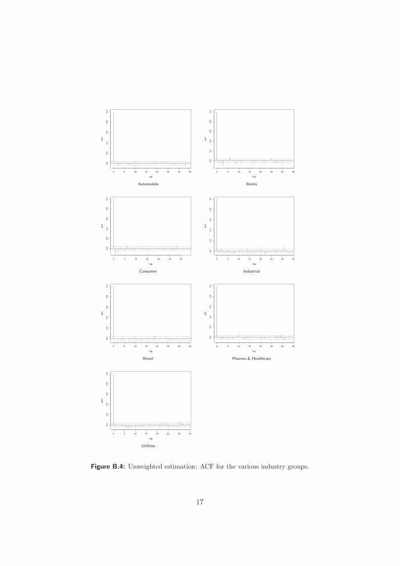
As outlined above, the non-parametric estimation results based on the gen-eralized market model (2) can only be considered reliable as long as theresiduals are neither autocorrelated nor heteroscedastic: Figure B.4 showsthe autocorrelation function of the fitted residuals in the different industrygroups, with model (2) fitted under the assumption of uncorrelated errors.Apparently, there is no indication of autocorrelation which is also shown inthe Durbin Watson statistics provided in Table B.4. Contrary, when look-ing for homoscedasticity Figure B.5 with fitted residuals ε2

jt plotted againsttime clearly gives the impression that the validity of homoscedasticity isquestionable. For this reason, the two-step estimation routine as suggestedin the previous section will be pursued.

The weighted estimation diagnostics for the various industry groups arereported in Table 3.1. As seen, both the parametric estimates reflecting themean value of systematic risk for the whole period under consideration aswell as the smooth terms are statistically significant at the 99%-level for eachindustry group. The mean value of systematic risk of the industry groups“Automobile” and “Banks” is close to unity, implying that, on average,these groups are affected by macroeconomic events to the same extent asthe average market. In contrast, all other groups are less responsive tooverall market movements. The smallest parametric beta-estimate of only0.55606 can be observed for the “Pharma & Healthcare” industry portfolio.Interestingly, on average there is no industry group that “overreacts” tomacroeconomic events, meaning that its parametric beta-estimate turns out

7

Industry Group Parametric Term Smooth Term

Coeff. Std.Error P-Value EDF P-Value

Automobile 0.98661 0.02348 < 0.001 16.71 < 0.001

Banks 0.93439 0.02079 < 0.001 14.55 < 0.001

Consumer 0.59742 0.02441 < 0.001 6.18 < 0.001

Industrial 0.77839 0.02119 < 0.001 15.45 < 0.001

Retail 0.67999 0.02279 < 0.001 4.37 0.0016

Pharma & H. 0.55606 0.02332 < 0.001 4.32 < 0.001

Utilities 0.73886 0.02155 < 0.001 15.95 < 0.001

Table 3.1: Weighted estimation results for the different industry groups

to be greater than one.However, as illustrated in Figure 3.1, the estimated beta-coefficients are

far from being stable over time and significantly deviate from their respectivemean values, especially during the period of 1996 – 2002. To be more precise,the estimation results roughly subdivide the industry groups into two classesas far as the volatility of the time-path of systematic risk is concerned:

One class comprises the industry groups “Automobile”, “Banks”, “In-dustrial” and “Utilities” with each having a (comparably) highly volatilebeta-coefficient. In contrast, the various beta-coefficients of the industrygroups “Consumer”, “Retail” as well as “Pharma & Healthcare” are exposedto a comparably small degree of time-variation. Strictly speaking, the esti-mated beta-paths “smoothly” decrease over time with troughs around theyears 2000 and 2001.

Especially for the industry groups with highly volatile beta-coefficients, arelationship between the time-path of systematic risk and the overall marketconditions can be seen. Figure 3.2 captures the return on the CDAX as asmooth function of time14. Denoting periods of average returns greater thanzero as up- or bull markets, and periods of average returns smaller thanzero as down- or bear markets, the following pattern can be observed: Forthese industry groups beta-coefficients tend to move counter-cyclically withrespect to the state of the market: on average, the respective beta-coefficientsare large in bear markets and small in bull markets. This also means thatinvestors focussing on these groups receive a higher risk-premium in periodsof substantial downside variation than in periods of upside variation.

More precisely, during the bearish market phases A, C and E as de-14The smooth function is based on an estimated gam-model of the form rMt = f(t)+ εt

using 14 degrees of freedom.

8

1992 1994 1996 1998 2000 2002

0.0

0.5

1.0

1.5

Date

s(D

ate,

16.7

1)

1992 1994 1996 1998 2000 2002

0.0

0.5

1.0

1.5

Date

s(D

ate,

14.5

5)

Automobile BanksMaximum basis dimension: k=20 Maximum basis dimension: k=20

1994 1996 1998 2000 2002

0.0

0.5

1.0

1.5

Date

s(D

ate,

6.18

)

1992 1994 1996 1998 2000 2002

0.0

0.5

1.0

1.5

Date

s(D

ate,

15.4

5)

Consumer IndustrialMaximum basis dimension: k=10 Maximum basis dimension: k=20

1992 1994 1996 1998 2000 2002

0.0

0.5

1.0

1.5

Date

s(D

ate,

4.37

)

1992 1994 1996 1998 2000 2002

0.0

0.5

1.0

1.5

Date

s(D

ate,

4.32

)

Retail Pharma & HealthcareMaximum basis dimension: k=10 Maximum basis dimension: k=10

1992 1994 1996 1998 2000 2002

0.0

0.5

1.0

1.5

Date

s(D

ate,

15.9

5)

UtilitiesMaximum basis dimension: k=20

Figure 3.1: Estimated time-paths of βj + βj(t) for the various industry groups

9

1992 1994 1996 1998 2000 2002

−0.

004

−0.

003

−0.

002

−0.

001

0.00

00.

001

0.00

2

Date

s(D

ate,

14)

A B C D E

Figure 3.2: Trend of the returns on the CDAX performance index

picted in Figure 3.2, the respective beta-coefficients of the industry groups“Automobile”, “Banks”, “Industrial” and “Utilities” are large or, at least,exhibit an upward trend. Conversely, the bullish market phases B and Dare associated with smaller beta-coefficients as far as these industry groupsare concerned.

3.3 Focussed Estimates

In order to cross-validate the suggested counter-cyclical behavior of betafor these industry groups, it seems helpful to focus on a reduced data-range.This is advisable since the estimation results are based on “global” concepts,that is to say smoothness is refined to as smoothness over the full range oftime15. As a consequence, local structures might be appropriately exhib-ited. Hence, we subsequently concentrate on a reduced estimation intervalcovering the market phases C, D and E as denoted in Figure 3.2.

Considering the various time-paths of systematic risk for the industrygroups “Automobile”, “Banks”, “Industrial” and “Utilities” in the reducedestimation interval in Figure 3.3, the suggested counter-cyclical behavior ofthe beta-coefficient becomes even more evident. All of them exhibit a smallor at least decreasing beta-coefficient during the bullish market phase D anda large or increasing beta-coefficient during the bear market environmentsC and E, respectively. Thus, the estimation results based on the reduced

15Spline smoothing in contrast to local smoothing is a global optimization problem. SeeHastie and Tibshirani (1990)

10

sample support the suggestion of a counter-cyclical behavior of the beta-coefficient for these industries.

1998 1999 2000 2001 2002 2003

0.0

0.5

1.0

1.5

Date

s(D

ate,

14.6

7)

C D E

1998 1999 2000 2001 2002 2003

0.5

1.0

1.5

Date

s(D

ate,

15.2

1)

C D E

Automobile BanksMaximum basis dimension: k=20 Maximum basis dimension: k=20

1998 1999 2000 2001 2002 2003

0.2

0.4

0.6

0.8

1.0

Date

s(D

ate,

10.6

)

C D E

1998 1999 2000 2001 2002 2003

−0.

50.

00.

51.

01.

5

Date

s(D

ate,

16.2

8)

C D E

Industrial UtilitiesMaximum basis dimension: k=20 Maximum basis dimension: k=20

Figure 3.3: Estimated time-paths of βj + βj(t) between 1998 and 2003

Of course, since the beta-coefficient of the market (portfolio) is, by def-inition, equal to one, there must also be some industry groups that exhibitthe exact opposite behavior. However, as far as our industry sample isconcerned, there is no evidence that such industry groups are included.

3.4 Performance Comparison

Finally, one aspect remains worth addressing: Even though the non-parametric estimates as presented so far reveal several “neat” results and in-sights into the time-path of systematic risk and thus indirectly acknowledgethe non-parametrical estimation technique as a useful tool for estimatingbeta-coefficients, the real gains in estimation accuracy still remain to beunknown. Therefore, this section aims to quantify the realized gains in esti-mation accuracy by measuring the improvements in fit over the conventionalordinary least-squares approach for constant beta-estimates. Generally, two

11

measures should be compared: first, the adjusted R2 as a measure of over-all fit, and secondly the Generalized Cross Validation (GCV)-criterion. TheGCV-criterion approximates the mean-squared error and hence accounts forboth bias and variance of an estimate. The objective is to reduce the GCVfunction16.

The results are reported in Table 3.2. Overall, they show gains in accu-racy for each industry group in terms of a higher R2 and lower GCV-scorewhen beta is allowed to vary. As expected, the largest improvements can beobserved for those industry groups whose betas are exposed to a high de-gree of time-variation, especially for the industries “Automobile”, “Banks”and “Utilities”. Thus, the non-parametric estimation technique as appliedin this analysis can be considered a useful tool for estimating time-varyingbeta-coefficients. Moreover, it provides a comprehensible alternative com-pared to the existing time-series approaches for these estimation purposes.

Industry Group Constant Beta Time-Varying Beta

R2(adj) GCV R2(adj) GCV

Automobile 0.525 1.03230 0.564 0.97797

Banks 0.550 1.04040 0.583 0.98471

Consumer 0.202 1.01920 0.225 0.99640

Industrial 0.377 1.01440 0.391 0.99495

Retail 0.278 0.99793 0.284 0.99398

Pharma & H. 0.210 0.99891 0.215 0.99100

Utilities 0.320 1.01610 0.341 0.99893

Table 3.2: Performance comparison between constant and time-varying beta-estimates

4 Conclusion

Our empirical results reveal that the German stock market exhibits symp-toms of time-varying beta-coefficients. This insight is in accordance withprevious studies that have found evidence of beta-instability in various othercountries. However, this study differs from preceding research in the methodapplied in order to estimate the time-path of beta. While most studies haveestimated beta as a time-series process using the Kalman filter, we focus on anon-parametric estimation technique that allows to treat the beta-coefficient

16See also Appendix C.

12

as an unspecified function of time. Compared to the existing time-seriesmodels, such an approach is not only more intuitive and thus quite easy tounderstand, the corresponding model can also be fitted to data in a com-fortable manner, as shown in Appendix A. Moreover, heteroscedasticity iseasily accommodated in the same model framework.

Due to the flexibility of the model by treating the beta-coefficient asan unspecified function of time, we were able to identify several industrygroups as being counter-cyclically related to the state of the market as faras their systematic risk exposure is concerned: on average, betas tend tobe significantly larger in bear-markets than in bull-markets for the groups“Automobile”, “Banks”, “Industrial” as well as “Utilities”.

With respect to the importance of the beta-coefficient in modern fi-nance, the results of this paper might be helpful in two regards. On the onehand, non-parametric estimation techniques whose real strengths are stillunderrated in many economic disciplines are shown to provide a potentialalternative to the more complicated time-series approaches for estimatingtime-varying beta-coefficients. On the other hand, the empirical analysisreveals significant insight into the time-path of systematic risk for a varietyof industry groups at the German stock market. Among the most importantfinding is the counter-cyclical behavior of some industry groups’ beta coeffi-cients with respect to the state of the market. For instance, with knowledgeof this kind beta-predictions could simply be used to adjust for the expec-tations of future market conditions.

13

A R-Commands

Software package R is an open source software which can be downloadedfree of charge from http://www.r-project.org. The routines used in thispaper are implemented in the mgcv package also available from the aboveweb page. A general overview about the features of R is found for instancein Dalgaard (2002).

The generalized market model (2) can be estimated using the followingR-command:

> gam(Rj ∼ RM + s(t, by=RM))

The by-argument ensures that the smooth function βj(t) gets multiplied bythe predictor RMt. The formula further indicates that the estimated time-path of the beta-coefficient is represented by a constant plus a smooth ef-fect. This is because the individual smooth functions in a varying-coefficientmodel have to be constrained to have zero mean. Otherwise the effects ofthe covariates would not be identifiable. Since mgcv’s gam() automaticallyaccounts for this constraint, regardless of the number of covariates in themodel, the resulting smooth functions are centered around zero. However,for model (2) this means that the estimate of the whole term βj(t)RMt iscentered around zero, even though its “actual” mean value might differ fromzero. Therefore, the term RMt must be included as well whose parametric es-timate can be regarded as the mean value of beta for the whole period underconsideration. Thus, depending on the time period the smooth componenteither increases or reduces the estimated mean value of the beta-coefficient.

A.1 Autocorrelated Residuals

One way to cope with autocorrelated residuals would be to determine thesmoothing parameter by hand. In such a case, the appropriate gam()-formula is as follows:

> gam(Rj ∼ RM + s(t, by=RM, knots|f))

The parameter knots must be replaced by the desired number of knots: themore knots are placed the more flexible the fit becomes and vice versa.

14

A.2 Heteroscedasticity

The two-step estimation approach for coping with heteroscedastic residualsfirst requires to fit the generalized additive gamma model (5). In R this canbe done using the following command:

> gam(r.squared ∼ s(t), family=Gamma)

with the family-argument specifying the desired response probability dis-tribution. After having constructed the appropriate weights, the weightedmarket model can be fitted to data by:

> gam(Rj ∼ RM + s(t, by=RM), weights=wj)

with the weights-argument ensuring to incorporate the vector of the con-structed weights wjt.

15

B Data Summary and Estimation Diagnostics

Company 1st Obs. Company 1st Obs.

Automobile Banks

Volkswagen AG 04/1991 Bayer. H.- und Vereinsbank AG 04/1991

Daimler Chrysler AG 04/1991 Commerzbank AG 04/1991

BMW AG 03/1993 Deutsche Bank AG 04/1991

Continental AG 03/1993 IKB Dt. Industriebank AG 01/1996

Consumer Retail

Adidas-Salomon AG 11/1995 Celesio AG 01/1996

Henkel KGaA 03/1993 Douglas Holding AG 04/1995

Wella AG 01/1996 Fielmann AG 01/1996

Beiersdorf AG 11/1996 Karstadt Quelle AG 04/1991

Puma AG 07/1996 Metro AG 07/1998

Pharma & Healthcare Industrial

Altana AG 05/1996 Deutz AG 11/1992

Fresenius Medical Care AG 10/1996 Linde AG 04/1991

Schering AG 06/1991 MAN AG 04/1991

Merck KGaA 10/1995 Rheinmetall AG 03/1998

Schwarz Pharma AG 02/1996 MG Technologies AG 10/1992

Thyssen Krupp AG 04/1991

Utilities IWKA AG 08/1996

E.ON AG 03/1993 Jenoptik AG 10/1998

RWE AG 04/1991

Table B.3: Companies included in the analysis with dates of their first observation

Industry Group DW-statistic

Automobile 2.0167

Banks 2.0758

Consumer 2.1880

Industrial 2.0186

Retail 2.0102

Pharma & Healthcare 1.9751

Utilities 1.9457

Table B.4: Durbin Watson statistics for the various industry groups.

16

0 5 10 15 20 25 30 35

0.0

0.2

0.4

0.6

0.8

1.0

Lag

AC

F

0 5 10 15 20 25 30 35

0.0

0.2

0.4

0.6

0.8

1.0

Lag

AC

F

Automobile Banks

0 5 10 15 20 25 30

0.0

0.2

0.4

0.6

0.8

1.0

Lag

AC

F

0 5 10 15 20 25 30 35

0.0

0.2

0.4

0.6

0.8

1.0

Lag

AC

F

Consumer Industrial

0 5 10 15 20 25 30 35

0.0

0.2

0.4

0.6

0.8

1.0

Lag

AC

F

0 5 10 15 20 25 30 35

0.0

0.2

0.4

0.6

0.8

1.0

Lag

AC

F

Retail Pharma & Healthcare

0 5 10 15 20 25 30 35

0.0

0.2

0.4

0.6

0.8

1.0

Lag

AC

F

Utilities

Figure B.4: Unweighted estimation: ACF for the various industry groups.

17

1992 1994 1996 1998 2000 2002

−0.

06−

0.04

−0.

020.

000.

020.

040.

06

Date

Res

idua

ls

1992 1994 1996 1998 2000 2002

−0.

050.

000.

050.

10

Date

Res

idua

ls

Automobile Banks

1994 1996 1998 2000 2002

−0.

06−

0.04

−0.

020.

000.

020.

040.

06

Date

Res

idua

ls

1992 1994 1996 1998 2000 2002

−0.

06−

0.04

−0.

020.

000.

020.

040.

060.

08

Date

Res

idua

ls

Consumer Industrial

1992 1994 1996 1998 2000 2002

−0.

04−

0.02

0.00

0.02

0.04

0.06

Date

Res

idua

ls

1992 1994 1996 1998 2000 2002

−0.

050.

000.

050.

10

Date

Res

idua

ls

Retail Pharma & Healthcare

1992 1994 1996 1998 2000 2002

−0.

06−

0.04

−0.

020.

000.

020.

040.

06

Date

Res

idua

ls

Utilities

Figure B.5: Unweighted estimation: Residuals for the various industry groups.

18

1992 1994 1996 1998 2000 2002

−4

−2

02

4

Date

Res

idua

ls: A

utom

obile

1992 1994 1996 1998 2000 2002

−2

02

4

Date

Res

idua

ls: B

anks

Automobile Banks

1994 1996 1998 2000 2002

−4

−2

02

4

Date

Res

idua

ls: C

onsu

mer

1992 1994 1996 1998 2000 2002

−4

−2

02

4

Date

Res

idua

ls: I

ndus

tria

l

Consumer Industrial

1992 1994 1996 1998 2000 2002

−4

−2

02

4

Date

Res

idua

ls: R

etai

l

1992 1994 1996 1998 2000 2002

−6

−4

−2

02

4

Date

Res

idua

ls: P

harm

a &

Hea

lthca

re

Retail Pharma & Healthcare

1992 1994 1996 1998 2000 2002

−6

−4

−2

02

4

Date

Res

idua

ls: U

tiliti

es

Utilities

Figure B.6: Two-step weighted estimation: Residuals for the various industrygroups.

19

C Theoretical Notes on the Varying-Coefficient Model

It can be shown (see e.g. De Boor (1978, ch. 4)) that a weighted version ofthe minimization problem (3) can be written as

(Y −Xβ −Cb)T W (Y −Xβ −Cb) + λbTDb. (6)

with Y = (Rj1, . . . , RjT )T , X = (1, RM ) and RM = (RM1, . . . , RMT ).Matrix C is a n× p dimensional spline basis built from rows

Ct = RMt(B1(t), . . . , Bp(t)), t = 1, . . . , T

with Bl(t) as l-th spline basis. Finally, W = diag(wjt) is the diagonalmatrix of weights accounting for heteroscedasticity andD is a penalty matrixsteering with λ the smoothness of the resulting fit. Additional constraintson b are necessary to ensure identifiability, but for notational simplicity andsince technically these do not cause problems we ignore them here (see Wood(2000) for a more technical insight). Keeping the smoothing parameter λ

fixed, one gets an estimate for Θ = (β, b) via

Θ =

((XT

CT

)W (XC) + λdiag(0,D)

)−1 (XT

CT

)WY

=: MλY

Note that if weights wjt depend on Θ as well, iterated estimation is necessary.In our fitting process we however confine ourselves to a two stage fittingroutine only.

An important issue in non-parametric regression is the selection of anappropriate smoothing parameter. Choosing λ = 0 results in a wiggled es-timate while λ →∞ would yield a time constant beta-coefficient. A widelyaccepted method for smoothing parameter selection (see Hastie and Tibshi-rani (1990)) is minimizing Akaike’s information criterion (Akaike (1973)) orits relative the Generalized Cross Validation (Craven and Wahba (1979))

GCV (λ) =(Y −Xβ −Cb)T W (Y −Xβ −Cb) /T

[1− df(λ)/n]2

where df(λ) is a measure for the degree of freedom or for the complexity

20

of the fit, respectively. As motivated for instance in Hastie and Tibshirani(1990, ch. 3) a suitable choice for df(λ) is the trace of the ”hat” matrix,which here means

df(λ) = trace {Mλ(XC)}

Clearly, GCV (λ) does not allow for simple minimization, since ∂GCV (λ)/∂λ =0 does not provide an analytic solution. However, the simple idea of a New-ton Raphson procedure can be applied to solve the first order derivative.Details are provided in Wood (2000) and the procedure is implemented inR.

When working with any automatic smoothing parameter selection oneshould be aware that the routines usually have a large variability. In practi-cal terms this means, one should not blindly believe in the selected smooth-ing parameter and take the resulting fit for granted. Instead, one shouldvisually check the fit with different smoothing parameters. If differencesare minor, the automatic selected smoothing parameter can be accepted17.We followed this advice in our data example and found that the automaticselected smoothing parameters behaved satisfactory.

17See also Ruppert, Wand, and Carroll (2003b, ch. 5.4).

21

References

Akaike, H., 1973, “Information Theory and an Extension of the maximumlikelihood principle,” Second international symposium on information the-ory, pp. 267–281.

Alexander, G., and N. Chervany, 1980, “On the estimation and stability ofbeta,” Journal of Financial and Quantitative Analysis, 15, 123–137.

Altman, E., B. Jacquillat, and M. Levasseur, 1974, “Comparative analysisof risk measures: France and the United States,” Journal of Finance, 27,1495–1511.

Baesel, J., 1971, “On the assessment of risk: Some further considerations,”Journal of Finance, 27, 1491–1494.

Blume, M., 1971, “On the assessment of risk,” Journal of Finance, 24, 1–10.

Bowman, A., and A. Azzalini, 1997, Applied smoothing tecniques for dataanalysis . Oxford Statistical Science Series, Clarendon Press, Oxford.

Campbell, J., and J. Cochrane, 2000, “Explaining the poor performance ofconsumption-based asset pricing models,” Journal of Finance, 55, 1–16.

Cochrane, J., 2001, Asset pricing, Princeton University Press, Princeton.

Craven, P., and G. Wahba, 1979, “Smoothing noisy data with spline func-tions,” Numerical Mathematics, 31, 377–403.

Dalgaard, P., 2002, Introductory Statistics with R, Springer Verlag.

De Boor, C., 1978, A practical guide to Splines, Springer Verlag, New York.

Deutsche-Borse-Group, 2003, Leitfaden zu den Aktienindizes der DeutschenBorse.

Green, P., and B. Silverman, 1994, Nonparametric regression and general-ized linear models . Monographs on Statistics and Applied Probability,Chapman and Hall, London.

Grinblatt, M., and S. Titman, 2002, Financial markets and corporate strat-egy, McGraw-Hill/Irwin, New York, 2nd edn.

22

Gu, C., and G. Wahba, 1991, “Minimizing GCV/GML scores with mul-tiple smoothing parameters via the newton method,” SIAM Journal ofScientific and Statistical Computing, 12, 383–398.

Hastie, T., 1996, “Pseudosplines,” Journal of the Royal Statistical SocietyB, 58, 379–396.

Hastie, T., and R. Tibshirani, 1990, Generalized additive models . Mono-graphs on Statistics and Applied Probability, Chapman and Hall, Lon-don.

Hastie, T., and R. Tibshirani, 1993, “Varying-coefficient models,” Journalof the Royal Statistical Society B, 55, 757–796.

Kauermann, G., and J. Opsomer, 2004, “Generalized cross-validation forbandwidth selection of backfitting estimates in generalized additive mod-els,” Journal of Computational and Graphical Statistics, 13, 66–89.

Markowitz, H., 1952, “Portfolio selection,” The Journal of Finance, 12, 77–91.

McCullagh, P., and J. Nelder, 1989, Generalized linear models . Monographson Statistics and Applied Probability, Chapman and Hall, New York.

Opsomer, J., Y. Wang, and Y. Yang, 2001, “Nonparametric regression withcorrelated errors,” Statistical Science, 16, 134–153.

Roenfeldt, R., G. Griepentrong, and C. Pflaum, 1978, “Further evidence onthe stationarity of beta coefficients,” Journal of Financial and Quantita-tive Analysis, 13, 117–121.

Ruppert, D., M. Wand, and R. Carroll, 2003a, Semiparametric regression,Cambridge University Press, Cambridge.

Ruppert, R., M. Wand, and R. Carroll, 2003b, Semiparametric Regression,Cambridge University Press.

Schaefer, S., R. Brealey, S. Hodges, and H. Thomas, 1975, “Alternativemodels of systematic risk,” In Elton, E. & M. Gruber, eds, Internationalcapital markets, North Holland, Amsterdam, 150–161.

23

Semmler, W., 2003, Asset prices, booms and recessions: Financial markets,economic activity and the macroeconomy, Springer Verlag, Berlin.

Sharpe, W., 1963, “A simplified model for portfolio analysis,” ManagementScience, 9, 227–293.

Sharpe, W., 1964, “Capital asset prices: A theory of market equilibriumunder conditions of risk,” Journal of Finance, 19, 425–442.

Sharpe, W., 1970, Portfolio theory and capital markets . Series in Finance,McGraw-Hill, New York.

Theobald, M., 1981, “Beta stationarity and estimation period: Some analyt-ical results,” Journal of Financial and Quantitative Analysis, 16, 747–757.

Wells, C., 1995, The Kalman filter in Finance, Kluwer Academic Publishers,Dordrecht.

Wood, S., 2000, “Modelling and smoothing parameter selection with mul-tiple quadratic penalties,” Journal of the Royal Statistical Society B, 50,413–436.

Wood, S., 2001, “mgcv: GAMs and generalized ridge regression for R,” R

News, 1/2, 20–25.

24