estimates of stock origin for bluefin tuna … · caught in western atlantic fisheries from 1975 to...

SCRS/2015/041 Collect. Vol. Sci. Pap. ICCAT, 72(6): 1376-1393 (2016)

1376

ESTIMATES OF STOCK ORIGIN FOR BLUEFIN TUNA

CAUGHT IN WESTERN ATLANTIC FISHERIES FROM 1975 TO 2013

Alex Hanke1, Dheeraj Busawon1 Jay R. Rooker2 and Dave H. Secor3

SUMMARY

Estimates of stock origin are given for Bluefin tuna caught in western Atlantic fisheries from

1975 to 2013. Classification models were developed on the stable isotope ratios of carbon and

oxygen using both Random Forest and linear and quadratic discriminant analysis for

classification.

RÉSUMÉ

Les estimations de l'origine du stock sont présentées pour le thon rouge capturé par les

pêcheries de l'Atlantique Ouest entre 1975 et 2013. Des modèles de classification ont été

élaborés sur la base des isotopes stables de carbone et d'oxygène au moyen de méthodologies

des forêts aléatoires, d'une analyse discriminante linéaire, d'une analyse discriminante

quadratique aux fins de la classification.

RESUMEN

Se presentan estimaciones de origen del stock para el atún rojo capturado en pesquerías del

Atlántico occidental desde 1975 hasta 2013. Se desarrollaron modelos de clasificación en las

ratios de isótopos estables de carbono y oxígeno usando análisis lineales discriminantes,

análisis cuadráticos discriminantes y metodologías de bosques aleatorios para la clasificación.

KEYWORDS

Discriminant analysis, RandomForest, bluefin tuna, natal origin, stable isotope ratios

1. Introduction

Currently, Bluefin tuna are managed as two separate stocks with no allowance for mixing between them. That is

not to say that mixing is not a concern or that methods to allow for mixing have not been applied in the past. The

fact that there is no allowance is strictly a function of the lack of mixing data.

Evidence of mixing can come from several sources, genetic analysis, otolith shape analysis, tagging studies and

otolith micro constituent analysis. Here we use otolith micro constituents as the basis for determining the natal

origin of stocks. The micro constituents are the isotopes of carbon and oxygen found in the part of the otolith

associated with the first year of life. Ratios of these isotope concentrations vary over the Bluefin tuna’s range but

these ratios measured at the earliest possible moment of life reflect its natal origin. To date, science accepts the

presence of two spawning grounds; the Gulf of Mexico and the Mediterranean Sea.

Bluefin tuna from the western management zone are hatched in the Gulf of Mexico while the eastern fish are

hatched in the Mediterranean Sea and because Bluefin are credited with spawning fidelity we can expect them to

return. However, between hatching and spawning, they are free to occur almost anywhere else and this study

attempts to predict the stock or natal origin of Bluefin caught in the western portion of the Atlantic Ocean.

1 Fisheries & Oceans Canada, Biological Station, 531 Brandy Cove Road, St. Andrews, NB E5B 2L9 CANADA. Email address of lead

author: [email protected]. 2 Department of Marine Biology, Texas A&M University, 1001 Texas Clipper Road, Galveston, Texas 77553 USA. 3 Chesapeake Biological Laboratory, University of Maryland Center for Environmental Science.

1377

2. Methods

2.1 Data source

Two data sources were required for this analysis. The first is the baseline data on which the classification models

were fit and the second is the samples for which the stock or natal origin is predicted.

The samples were collected from fish harvested off the New England coast and north as far as Newfoundland

(NL) (Table 1). The New England samples were collected in the late 1970’s and the majority of samples were

collected recently (2010-2013) from the Gulf of St. Lawrence (GSL) and Atlantic coast of Nova Scotia (NS). St.

Margret’s Bay (SMB) is on the Atlantic coast but it is treated as a separate region.

The baseline data were made available by Rooker et al. (2014) and can be accessed at: www.int-

res.com/articles/suppl/m504p265_supp.xls.

2.2 Biological sampling

The details of the catch from New England and Virginia dating back to the late 1970s are not known. We assume

that these samples were collected by the same methods as the more modern samples described below.

Bluefin tuna heads labeled with a unique commercial tag number were stockpiled by fishermen and co-ops, and

then sampled by a field technician. Sampling consisted of extracting sagittal otoliths from Atlantic Bluefin tuna

heads and taking snout length measurements (Busawon et al. 2013).

The commercial tag number was linked to commercial databases to obtain catch (e.g. location) and size

information. In some cases, the curved fork length of the fish was not reported in commercial databases or the

label with the commercial tag number was lost. In these instances, we used monthly length-weight conversion

(ICCAT 2006) and snout length conversion (Secor et al. 2014) to calculate curved fork length.

2.3 Natal origin

A single otolith (right or left) from each sample was embedded in resin and a 2.0 mm thick section was cut from

the center containing the juvenile portion of the otolith. A template from measured juvenile otolith sections was

used to identify the first annulus, which increased the consistency of the cut location (Rooker et al. 2008).

Carbonate material was milled from the identified region using a New Wave Micromill©. Samples were

analyzed for δ18O and δ13C (±0.1‰ and ±0.6‰ respectively for δ18O and δ13C) at the University of Arizona

Environmental Isotope Laboratory. For more detail on the otolith processing methodology see Schloesser et al.

(2010) and Secor et al. (2013).

Otolith δ18O and δ13C from historical samples collected in New England, Virginia, Caraquet and Miscou

(1975-1977) were corrected for the Suess Effect prior to analysis (Schloesser et al. 2009). Powdered otolith

extracted from the otolith core was analyzed to determine the isotropic differences of 13C and 18O from their

isotropic standards. The calculation is:

𝛿𝐴𝑋𝑆𝑇𝐷 =𝑅𝑆𝑎𝑚𝑝𝑙𝑒

𝐴

𝑅𝑆𝑇𝐷𝐴 − 1

Here δ expresses the abundance of isotope A of element X in a sample relative to the abundance of that same

isotope in the isotopic standard (McKinney et al. 1950).

2.4 Data analysis

Classification of the samples to a stock was accomplished using linear discriminant (LDA), quadratic

discriminant (QDA) (Bischel et al. 2014, Venables and Ripley 2002) and randomForest (Liaw and Wiener 2002)

classifiers. The QDA used here is equivalent to the conditional maximum likelihood estimate procedure HISEA

(Millar 1990; http://www.stat.auckland.ac.nz/~millar/mixedstock/code.html) used by other authors.

http://www.stat.auckland.ac.nz/~millar/mixedstock/code.html

1378

2.4.1 Linear and quadratic discriminant analysis models

Base models for both LDA and QDA used both δ13C and δ18O as the primary variables distinguishing eastern

from western samples.

The linear and quadratic discriminant analysis approaches differ with respect to assumptions made about the

form of the covariance matrix for each class. Unlike in LDA, QDA assumes that the covariance matrix can be

different for each class. Should a class have greater dispersion; cases will be over classified in it. Past analyses

using the same baseline data (Rooker et al. 2014) have assumed that the covariance matrices are different and

thus opted for the QDA approach. The evidence suggests that a QDA is justified but we fit both models

nonetheless. Multicollinearity between the variables and normality of the variables within the groups was also

assessed.

In each case, the performance of the learning algorithm was assessed using 3-fold cross validation and bootstrap

resampling (n=500). Under cross validation the model is trained on 2 of the 3 data partitions and tested on the

third while preserving the proportion of observations in each class. Under bootstrap resampling, a sample is

drawn with replacement for training and any observations not in the training set are used for testing for each run.

Performance is evaluated on the basis of the value of the aggregate false positive rate (fpr), false negative rate

(fnr) and the mean misclassification error (mmce). Performance was re-evaluated after optimizing the

classification threshold.

The resampling was conducted using the observed base sample probabilities and equalized base sample

probabilities. Equalization was achieved by over sampling the minority class (West). An optimal classification

threshold was chosen such that the fpr, fnr and mmce were minimized. The performance of the models under

resampling was compared to a model trained on all the data so that the sensitivity to over fitting could be

assessed.

The primary predictors were δ13C and δ18O; however models were also trained on an expanded basis by

including both quadratic and cross-product terms (i.e. δ13C2, δ18O2 and δ13Cxδ18O). This introduced 3 new

dimensions with a nonlinear basis.

2.4.2 RandomForest models

A randomForest model was trained on the base observations of δ13C and δ18O with no attempt to expand the

basis. Each classifier was based on 500 trees with one variable tried at each split. Given that the base observation

probabilities favoured the East, equal sample sizes were specified to reduce the emphasis of this class during

training and, through class weighting factors, more priority was given to δ18O in the fitting. Tuning was

performed to determine the optimum threshold value for assigning each sample’s class probability to a class.

Resampling was not explicitly conducted because training on a subset of the data and testing on the remainder is

intrinsic to the randomForest algorithm. This makes randomForest resistant to over fitting.

3. Results Box's M-test for homogeneity of covariance matrices indicated that the covariance matrices were heterogeneous (Chi-Sq (approx.) = 54.3, df = 3, p-value = 0). Normality of the variables within groups and multicollinearity were not issues. 3.1 Discriminant analyses Both LDA and QDA were used on training sets of the base data to predict the origin of each base observation. The base observations did not have equal probabilities (P(East) =0.56) and consequently the effect of balancing the base observation probabilities was determined in combination with the type of resampling (cross-validation, bootstrap) and setting a threshold value for prediction. The default threshold value is 0.5. Tables 2 through 5 contrast the resampling methods, the effect of unequal base observation probabilities and linear versus quadratic DA. The performance measures (fpr, fnr, mmce) for QDA and LDA are similar across these comparisons. The mean misclassification error is consistently about 18% with a larger false positive rate. Since the positive class is “East”, this would indicate that western fish are being classed as being eastern to a greater degree than the reverse. The difference in rates is larger when the base observation probabilities are unequal. The last row of the tables provides the proportion of all the misclassified base observations by class and despite the “East” being the majority class; more western fish are classified as eastern because of the large fpr.

1379

Estimating the performance measures over a range of threshold values provides the threshold for which the

predicted posterior probabilities will classify the base observations into classes with a minimum mean

misclassification error and roughly equal false positive and negative rates. Tables 6 through 9 contrast the

resampling methods, the effect of unequal base observation probabilities and linear versus quadratic DA under

optimum threshold values. The optimum threshold value is higher when the base observation probabilities are

unequal (.65 vs .6 for LDA; .68 vs .62 for QDA). Again, both QDA and LDA have very similar performance

metrics and indeed the mmce is similar to models trained using the default threshold of 0.5. Now that the fpr and

fnr are balanced the majority of misclassified fish are due to eastern base observations misclassified as western

because “East” is the majority class. Consequently the proportion of misclassified fish is similar to the base

observation probabilities.

The potential for over fitting was evaluated by fitting models to all the base data. Tables 10 and 11 contrast the

effect of unequal base observation probabilities when predictions are based on a threshold value which balances

the fpr and fnr. Performance measures were not that different from what was estimated in Tables 6 through 9

and that suggests predictions on the sample data will be insensitive to the effects of over fitting. There is very

little difference between the performance of QDA and LDA and correcting for unequal base observation

probabilities had little impact on performance as well.

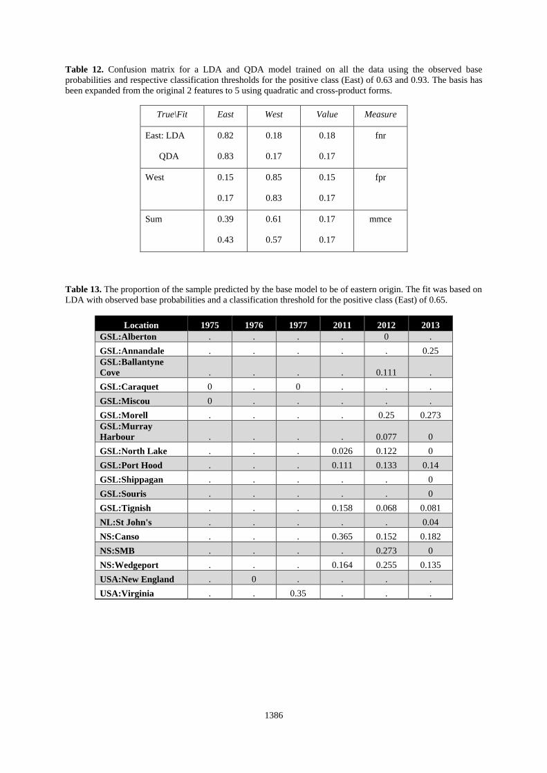
Fits to a LDA and QDA model with an expanded basis show that the extra variables do not improve the

performance of the classifier (Table 12) relative to full models with only two variables. In fact, a test of the

information gain associated with including each variable indicates that δ13C and δ13C2 contributes nothing and

that each of the other features (δ18O, δ18O2 and δ13Cxδ18O) are similar in importance.

Given that the LDA and QDA models fit to all the base data without equalizing the base observation

probabilities provided the best overall performance, the origin of the samples was predicted using the threshold

values that balanced the false positive and false negative error rates. Tables 13 and 14 provide the proportion of

the sample of eastern origin by year and sample location and Tables 15 and 16 give the regional estimates in

each year. Despite similar training errors, QDA predicts fewer eastern fish in the sample than LDA and this

discrepancy is partially a function of δ13C in the sample unlike δ13C in the base observations. A LDA fit to only

the δ18O base observations provides estimates of eastern fish in the sample similar to those provided by a QDA

model trained on both δ18O and δ13C.

3.2 RandomForest analysis

As with the LDA and QDA analyses, the classification error by class was affected by the unequal base

observation probabilities. Table 17 shows the biased fit to the majority class (East) and similar classification

errors when sample sizes are equal. However, the total model misclassification error (OOB=out-of-bag error

rate) is similar whether you correct for the unequal sample sizes or not. The accuracy is identical to what was

achieved using LDA or QDA.

Through a tuning process it was determined that the cutoff or threshold applied to the predicted class

probabilities yielded optimal sensitivity and specificity at 0.474 rather than at the default of 0.5. The predicted

origin of the samples (Table 18) was similar to results from QDA at a coarse spatial resolution. At a finer spatial

resolution (Table 19) the difference between a RandomForest and QDA classifier was more evident at particular

locations, though generally there was still good agreement.

Partial dependence plots (Figure 1) show the marginal effect of δ18O and δ13C on determining class probability.

A clear dependence exists between the class probabilities and values of δ18O whereas there is an unclear

relationship for δ13C. Measures of predictor variable importance indicate that δ18O is 5 times more influential in

reducing the error of classification and more than 2 times more influential in reducing the node impurity.

RandomForest models trained on δ18O alone had and out-of-bag error (17%) similar to one with both stable

isotope ratios.

The relationship between the base observations used in training the classifier and the sample stable isotope

values is shown in Figure 2. While many of the sample values fall within the bivariate normal kernel density

distributions, many do not. The discrepancy differs by region and is more evident for the δ13C values. Figure 3

relates the isotope values to the sample year and to the base observations used in training. The annual values are

conditioned on the predicted origin of the samples to separate any trend from the changing balance of eastern

and western fish sampled. Generally the median values are trending with time and are outside the range of the

data used in training.

1380

The classifiers (LDA, QDA, and RandomForest) provide a probability of class membership (East or West) and

the cutoff or threshold provides the decision rule that assigns the sample to a particular class. Rather than

evaluate the mixing by region using the sample assignment, the relative mixing by region was expressed as

probability density distributions. Figure 4 indicates the degree to which the samples are eastern or western in

origin. Locations like Virginia have a fairly uniform distribution indicating the potential for good representation

by both stocks in the catch. This is in contrast with the Newfoundland (NL) samples which have a high

probability of being western in origin. The class probabilities can also be related to other features of the sample

and one of the more obvious attributes is the curved fork length of the fish (CFL). Figure 5 shows that shorter

fish are more likely to be eastern in origin and that the median probability by length class differs by region.

4. Discussion

Base observations of δ18O and δ13C for Bluefin tuna of known origin provided the basis for classifying Bluefin

tuna catch spanning multiple years and locations. Three classifiers performed equally well on the training data

with misclassification rates of 17%. However, predictions of sample origin were only comparable for QDA and

randomForest while LDA classified more fish as being eastern in origin. The bivariate distribution of the

predictors in the sample was shown to be outside the range of the base observation for a portion on the data

(Figure 7). Rooker et al. (2014) had a similar issue for samples collected in the central North Atlantic Ocean but

not in the eastern Atlantic where most fish were determined to be of eastern origin. So perhaps the extra

variability in the sample stable isotope values may be a western origin phenomenon tied to the greater age of

these and/or the outliers could be a function of a third spawning location. A concern that we are extrapolating the

predictions to sample data beyond the envelope of the base observations is diminished by the fact that it is more

evident for the carbon isotope which does not have any predictive power.

The source of the differences in the isotope values is not known but may be related to time trends in the stable

isotope ratios at the reference locations or to otolith milling bias. Given that the 4 to 8 year old fish are more like

the base then the 9 to 36 year olds, drift in the stable isotope ratios at the reference site may be likely (Figure 6).

This observation is supported by Schlosser et al (2009) who found that both carbon and oxygen isotopic

signatures varied significantly by year of birth for Bluefin tuna with d13C decreasing and d18O increasing.

Although, both δ18O and δ13C have been used as predictors in classification analyses on Bluefin tuna, it has been

shown that δ13C has very little discriminatory power and one can omit it without affecting the estimated mixing

rates or increasing the classification error. Introducing a quadratic form of δ13C or the interaction with δ18O did

not improve its overall importance to the fit.

Taken at face value, the mixing analysis shows that there may be annual trends in the occurrence of eastern fish

on the fishing grounds and these may relate to the movement of small sized tuna. There is also a strong

dependence on location and season which will require consistent high resolution sampling before mixing can be

thoroughly understood. Estimates of mixing for the Virginia samples from the late 1970s were consistent with

estimates provided by Secor et al. (2013) for North American school size tuna caught in the same area.

A model relating the class probabilities to the coarse spatial and temporal features of the sampling and the

attributes of the fish may be able to provide estimates of stock origin for the corresponding times and locations

of the northwest Atlantic catch. This is for later.

1381

References

Bischl B., Lang M., Richter J., Bossek J., Judt L., Kuehn T., Studerus E. and Kotthoff L. 2014. mlr: Machine

Learning in R. R package version 2.2. http://CRAN.R-project.org/package=mlr

Busawon D. S., Neilson J. D., Andrushchenko I., Hanke A.R., Secor D.H. and Melvin,G. 2014. Evaluation of

Canadian Sampling Program for Bluefin tuna, Results of Natal Origin Studies 2011-2012 and Assessment

of Length-weight Conversions. Col. Vol. Sci. Pap. ICCAT, 70(1): 202-219.

Liaw A. and Wiener M. 2002. Classification and Regression by randomForest. R News 2(3), 18-22.

McKinney C.R., McCrea J.M., Epstein S., Allen H.A. and Urey H.C. 1950. Improvements in mass spectrometers

for the measurement of small differences in isotope abundance ratios. Rev. Sci. Instrum. 21, 724-730.

Millar R.B. 1990. Stock composition program HISEA. www.stat.auckland.ac.nz/~millar/mixedstock/code.html

Rooker J.R., Secor D.H., DeMetrio G.D., Schloesser R., Block B.A. and Neilson J.D. 2008. Natal homing and

connectivity in Atlantic Bluefin tuna populations. Science 322: 742-744.

Rooker J.R, Arrizabalaga H., Fraile I., Secor D.H. and others. 2014. Crossing the line: migratory and homing

behaviors of Atlantic bluefin tuna. Mar Ecol Prog Ser 504:265-276.

Schloesser R.W., Rooker J.R, Louchuoarn P., Neilson J.D. and Secor D.H. 2009. Inter-decadal variation in

ambient oceanic δ13C and δ18O recorded in fish otoliths. Limnology and Oceanography 54(5): 1665-1668.

Schloesser R.W., Neilson J.D, Secor D.H., and Rooker J.R. 2010. Natal origin of Atlantic Bluefin tuna (Thunnus

thynnus) from the Gulf of St. Lawrence based on otolith δ13C and δ18O. Canadian Journal of Fisheries and

Aquatic Sciences 67: 563-569.

Secor D.H., Busawon D.S., Gahagan B., Golet W., Koob E., Neilson J.D. and Siskey M. 2014. Conversion

factors for Atlantic bluefin tuna fork length from measures of snout length and otolith mass. Collect. Vol.

Sci. Pap. ICCAT, 70(2): 364-367.

Secor D.H., Rooker J.R., Neilson J.D., Busawon D.S., Gahagan B. and Allman R. 2013. Historical Atlantic

Bluefin Tuna Stock Mixing within U.S. Fisheries, 1976-2012. Col. Vol. Sci. Pap. ICCAT, 69(2): 938-

946.

Venables W. N. and Ripley B.D. 2002. Modern Applied Statistics with S. Fourth Edition. Springer, New York.

ISBN 0-387-95457-0.

http://cran.r-project.org/package=mlr

1382

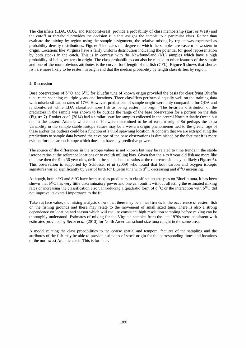
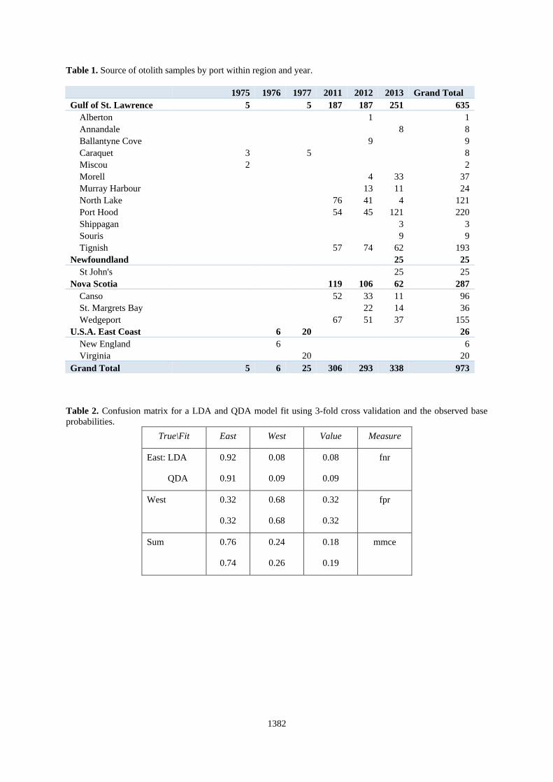
Table 1. Source of otolith samples by port within region and year.

1975 1976 1977 2011 2012 2013 Grand Total

Gulf of St. Lawrence 5

5 187 187 251 635

Alberton

1

1

Annandale

8 8

Ballantyne Cove

9

9

Caraquet 3

5

8

Miscou 2

2

Morell

4 33 37

Murray Harbour

13 11 24

North Lake

76 41 4 121

Port Hood

54 45 121 220

Shippagan

3 3

Souris

9 9

Tignish

57 74 62 193

Newfoundland

25 25

St John's

25 25

Nova Scotia

119 106 62 287

Canso

52 33 11 96

St. Margrets Bay

22 14 36

Wedgeport

67 51 37 155

U.S.A. East Coast

6 20

26

New England

6

6

Virginia

20

20

Grand Total 5 6 25 306 293 338 973

Table 2. Confusion matrix for a LDA and QDA model fit using 3-fold cross validation and the observed base

probabilities.

True\Fit East West Value Measure

East: LDA

QDA

0.92

0.91

0.08

0.09

0.08

0.09

fnr

West 0.32

0.32

0.68

0.68

0.32

0.32

fpr

Sum 0.76

0.74

0.24

0.26

0.18

0.19

mmce

1383

Table 3. Confusion matrix for a LDA and QDA model fit using 3-fold cross validation and equal base

probabilities.


East: LDA

QDA

0.88

0.88

0.12

0.12

0.12

0.12

fnr

West 0.26

0.29

0.74

0.71

0.26

0.29

fpr

Sum 0.63

0.65

0.37

0.35

0.18

0.19

mmce

Table 4. Confusion matrix for a LDA and QDA model fit using bootstrap resampling and the observed base

probabilities.


East: LDA

QDA

0.92

0.92

0.08

0.08

0.08

0.08

fnr

West 0.32

0.32

0.68

0.68

0.32

0.32

fpr

Sum 0.75

0.75

0.25

0.25

0.18

0.18

mmce

Table 5. Confusion matrix for a LDA and QDA model fit using bootstrap resampling and equal base

probabilities.


East: LDA

QDA

0.89

0.89

0.11

0.11

0.11

0.11

fnr

West 0.26

0.28

0.74

0.72

0.26

0.28

fpr

Sum 0.64

0.67

0.36

0.33

0.18

0.18

mmce

1384

Table 6. Confusion matrix for a LDA and QDA model fit using 3-fold cross validation, observed base

probabilities and respective classification thresholds for the positive class (East) of 0.65 and 0.68.


East: LDA

QDA

0.83

0.83

0.17

0.17

0.17

0.17

fnr

West 0.18

0.17

0.82

0.83

0.18

0.17

fpr

Sum 0.45

0.43

0.55

0.57

0.18

0.17

mmce

Table 7. Confusion matrix for a LDA and QDA model fit using 3-fold cross validation and equal base



East: LDA

QDA

0.81

0.82

0.19

0.18

0.19

0.18

fnr

West 0.16

0.19

0.84

0.81

0.16

0.19

fpr

Sum 0.39

0.45

0.61

0.55

0.18

0.18

mmce

Table 8. Confusion matrix for a LDA and QDA model fit using bootstrap resampling, observed base



East: LDA

QDA

0.84

0.82

0.16

0.18

0.16

0.18

fnr

West 0.16

0.17

0.84

0.83

0.16

0.17

fpr

Sum 0.43

0.42

0.57

0.58

0.16

0.17

mmce

1385

Table 9. Confusion matrix for a LDA and QDA model fit using bootstrap resampling, equal base probabilities

and respective classification thresholds for the positive class (East) of 0.60 and 0.62.


East: LDA

QDA

0.82

0.82

0.18

0.18

0.18

0.18

fnr

West 0.16

0.17

0.84

0.83

0.16

0.17

fpr

Sum 0.40

0.43

0.60

0.57

0.17

0.18

mmce

Table 10. Confusion matrix for a LDA and QDA model trained on all the data, observed base probabilities and

respective classification thresholds for the positive class (East) of 0.65 and 0.68.


East: LDA

QDA

0.84

0.81

0.16

0.17

0.16

0.17

fnr

West 0.17

0.17

0.83

0.83

0.17

0.17

fpr

Sum 0.44

0.42

0.56

0.58

0.16

0.18

mmce

Table 11. Confusion matrix for a LDA and QDA model trained on all the data, equal base probabilities and

respective classification thresholds for the positive class (East) of 0.60 and 0.62.


East: LDA

QDA

0.82

0.81

0.18

0.19

0.18

0.19

fnr

West 0.17

0.16

0.83

0.84

0.17

0.16

fpr

Sum 0.41

0.39

0.59

0.61

0.17

0.17

mmce

1386

Table 12. Confusion matrix for a LDA and QDA model trained on all the data using the observed base

probabilities and respective classification thresholds for the positive class (East) of 0.63 and 0.93. The basis has

been expanded from the original 2 features to 5 using quadratic and cross-product forms.


East: LDA

QDA

0.82

0.83

0.18

0.17

0.18

0.17

fnr

West 0.15

0.17

0.85

0.83

0.15

0.17

fpr

Sum 0.39

0.43

0.61

0.57

0.17

0.17

mmce

Table 13. The proportion of the sample predicted by the base model to be of eastern origin. The fit was based on

LDA with observed base probabilities and a classification threshold for the positive class (East) of 0.65.

Location 1975 1976 1977 2011 2012 2013

GSL:Alberton . . . . 0 .

GSL:Annandale . . . . . 0.25

GSL:Ballantyne

Cove . . . . 0.111 .

GSL:Caraquet 0 . 0 . . .

GSL:Miscou 0 . . . . .

GSL:Morell . . . . 0.25 0.273

GSL:Murray

Harbour . . . . 0.077 0

GSL:North Lake . . . 0.026 0.122 0

GSL:Port Hood . . . 0.111 0.133 0.14

GSL:Shippagan . . . . . 0

GSL:Souris . . . . . 0

GSL:Tignish . . . 0.158 0.068 0.081

NL:St John's . . . . . 0.04

NS:Canso . . . 0.365 0.152 0.182

NS:SMB . . . . 0.273 0

NS:Wedgeport . . . 0.164 0.255 0.135

USA:New England . 0 . . . .

USA:Virginia . . 0.35 . . .

1387


QDA with observed base probabilities and a classification threshold for the positive class (East) of 0.68.

Location 1975 1976 1977 2011 2012 2013



GSL:Ballantyne

Cove . . . . 0.111 .



GSL:Morell . . . . 0.25 0.182

GSL:Murray

Harbour . . . . 0 0

GSL:North Lake . . . 0.026 0.073 0

GSL:Port Hood . . . 0.111 0.133 0.132



GSL:Tignish . . . 0.158 0.054 0.032

NL:St John's . . . . . 0.04

NS:Canso . . . 0.365 0.061 0.091

NS:St. Margret’s Bay . . . . 0.182 0

NS:Wedgeport . . . 0.149 0.216 0.081




LDA with observed base probabilities and a classification threshold for the positive class (East) of 0.65.

Region 1975 1976 1977 2011 2012 2013

GSL 0 . 0 0.09 0.10 0.13

NL . . . . . 0.04

NS . . . 0.25 0.21 0.11

SMB . . . . 0.27 .

USA . 0 0.35 . . .


QDA with observed base probabilities and a classification threshold for the positive class (East) of 0.68.

Region 1975 1976 1977 2011 2012 2013

GSL 0 . 0 0.09 0.08 0.10

NL . . . . . 0.04

NS . . . 0.24 0.15 0.06

SMB . . . . 0.18 .

USA . 0 0.35 . . .

1388

Table 17. Confusion matrix for a Random Forest classifier with and without sample size correction and class

weighting. The threshold for classification was {0.5, 0.5}.


East: without

with

129

124

21

26

0.14

.17

ce

West 24

18

91

97

0.21

0.16

ce

Sum 0.17

0.17

OOB

Table 18. The proportion of the sample predicted by the base model to be of eastern origin within broad

geographical regions by year. The fit was based on a Random Forest classifier with equal sample sizes per class

and heavier class weights on δ18O. The threshold for classification was {0.53, 0.47}.

Region 1975 1976 1977 2011 2012 2013

GSL 0 . 0 0.07 0.08 0.10

NL . . . . . 0.04

NS . . . 0.22 0.14 0.06

SMB . . . . 0.14 .

USA . 0 0.35 . . .

1389

Table 19. The proportion of the sample predicted by the base model to be of eastern origin for detailed locations

within each year. The fit was based on a Random Forest classifier with equal sample sizes per class and heavier

class weights on δ18O. The threshold for classification was {0.53, 0.47}.

Location 1975 1976 1977 2011 2012 2013



GSL:Ballantyne

Cove . . . . 0.111 .



GSL:Morell . . . . 0 0.212

GSL:Murray

Harbour . . . . 0 0

GSL:North Lake . . . 0.013 0.098 0

GSL:Port Hood . . . 0.074 0.133 0.124



GSL:Tignish . . . 0.14 0.054 0.032

NL:St John's . . . . . 0.04

NS:Canso . . . 0.346 0.091 0.091

NS:SMB . . . . 0.136 0

NS:Wedgeport . . . 0.119 0.176 0.081



Figure 1. Partial dependence plots showing the marginal effect of the randomForest predictors on the class

probability.

1390

Figure 2. The predicted origin of the samples by a Random Forest classifier in relation to the observed isotope

ratio values of both the sample (points) and the base observations (polygons).

Figure 3. Trends in stable isotope values for samples by predicted stock origin. The base observations used in

training are included as a reference.

1391

Figure 4 (cont.). Trends in stable isotope values for samples by predicted stock origin. The base observations

used in training are included as a reference.

Figure 5. The probability density distributions by catch location for the predicted class probability.

1392

Figure 6. The relationship between the predicted class probability and curved fork length by catch location.

Figure 7. Sample stable isotope ratios relative to the base for different aged fish.

1393

Figure 8. The relationship between the base observations and samples. 95% and 68% confidence ellipses for

eastern and western base observations are red and blue, respectively, while the sample is green.

estimates of stock origin for bluefin tuna … · caught in western atlantic fisheries from 1975 to...

Documents