essentials of stochastic processes - department of mathematics
TRANSCRIPT

i
Essentials of Stochastic Processes
Rick Durrett
30
40
50
60
70
10‐Sep
10‐Jun
10‐May
at expiry
0
10
20
500 520 540 560 580 600 620 640 660 680 700
Almost Final Version of the 2nd Edition, December, 2011
Copyright 2011, All rights reserved.

ii
Preface
Between the first undergraduate course in probability and the first graduatecourse that uses measure theory, there are a number of courses that teachStochastic Processes to students with many different interests and with varyingdegrees of mathematical sophistication. To allow readers (and instructors) tochoose their own level of detail, many of the proofs begin with a nonrigorousanswer to the question “Why is this true?” followed by a Proof that fills inthe missing details. As it is possible to drive a car without knowing about theworking of the internal combustion engine, it is also possible to apply the theoryof Markov chains without knowing the details of the proofs. It is my personalphilosophy that probability theory was developed to solve problems, so most ofour effort will be spent on analyzing examples. Readers who want to master thesubject will have to do more than a few of the twenty dozen carefully chosenexercises.
This book began as notes I typed in the spring of 1997 as I was teachingORIE 361 at Cornell for the second time. In Spring 2009, the mathematicsdepartment there introduced its own version of this course, MATH 474. Thisstarted me on the task of preparing the second edition. The plan was to havethis finished in Spring 2010 after the second time I taught the course, but whenMay rolled around completing the book lost out to getting ready to move toDurham after 25 years in Ithaca. In the Fall of 2011, I taught Duke’s versionof the course, Math 216, to 20 undergrads and 12 graduate students and overthe Christmas break the second edition was completed.
The second edition differs substantially from the first, though curiously thelength and the number of problems has remained roughly constant. Throughoutthe book there are many new examples and problems, with solutions that usethe TI-83 to eliminate the tedious details of solving linear equations by hand.My students tell me I should just use MATLAB and maybe I will for the nextedition.
The Markov chains chapter has been reorganized. The chapter on Poissonprocesses has moved up from third to second, and is now followed by a treatmentof the closely related topic of renewal theory. Continuous time Markov chainsremain fourth, with a new section on exit distributions and hitting times, andreduced coverage of queueing networks. Martingales, a difficult subject forstudents at this level, now comes fifth, in order to set the stage for their use ina new sixth chapter on mathematical finance. The treatment of finance expandsthe two sections of the previous treatment to include American options and thethe capital asset pricing model. Brownian motion makes a cameo appearancein the discussion of the Black-Scholes theorem, but in contrast to the previousedition, is not discussed in detail.
As usual the second edition has profited from people who have told me abouttypos over the last dozen years. If you find new ones, email: [email protected].
Rick Durrett

Contents
1 Markov Chains 11.1 Definitions and Examples . . . . . . . . . . . . . . . . . . . . . . 11.2 Multistep Transition Probabilities . . . . . . . . . . . . . . . . . 71.3 Classification of States . . . . . . . . . . . . . . . . . . . . . . . . 111.4 Stationary Distributions . . . . . . . . . . . . . . . . . . . . . . . 171.5 Limit Behavior . . . . . . . . . . . . . . . . . . . . . . . . . . . . 221.6 Special Examples . . . . . . . . . . . . . . . . . . . . . . . . . . . 29
1.6.1 Doubly stochastic chains . . . . . . . . . . . . . . . . . . . 291.6.2 Detailed balance condition . . . . . . . . . . . . . . . . . . 311.6.3 Reversibility . . . . . . . . . . . . . . . . . . . . . . . . . 351.6.4 The Metropolis-Hastings algorithm . . . . . . . . . . . . . 36
1.7 Proofs of the Main Theorems* . . . . . . . . . . . . . . . . . . . 391.8 Exit Distributions . . . . . . . . . . . . . . . . . . . . . . . . . . 441.9 Exit Times . . . . . . . . . . . . . . . . . . . . . . . . . . . . . . 491.10 Infinite State Spaces* . . . . . . . . . . . . . . . . . . . . . . . . 531.11 Chapter Summary . . . . . . . . . . . . . . . . . . . . . . . . . . 591.12 Exercises . . . . . . . . . . . . . . . . . . . . . . . . . . . . . . . 62
2 Poisson Processes 772.1 Exponential Distribution . . . . . . . . . . . . . . . . . . . . . . . 772.2 Defining the Poisson Process . . . . . . . . . . . . . . . . . . . . 802.3 Compound Poisson Processes . . . . . . . . . . . . . . . . . . . . 862.4 Transformations . . . . . . . . . . . . . . . . . . . . . . . . . . . 88
2.4.1 Thinning . . . . . . . . . . . . . . . . . . . . . . . . . . . 882.4.2 Superposition . . . . . . . . . . . . . . . . . . . . . . . . . 892.4.3 Conditioning . . . . . . . . . . . . . . . . . . . . . . . . . 90
2.5 Chapter Summary . . . . . . . . . . . . . . . . . . . . . . . . . . 912.6 Exercises . . . . . . . . . . . . . . . . . . . . . . . . . . . . . . . 92
3 Renewal Processes 1013.1 Laws of Large Numbers . . . . . . . . . . . . . . . . . . . . . . . 1013.2 Applications to Queueing Theory . . . . . . . . . . . . . . . . . . 106
3.2.1 GI/G/1 queue . . . . . . . . . . . . . . . . . . . . . . . . 1063.2.2 Cost equations . . . . . . . . . . . . . . . . . . . . . . . . 1073.2.3 M/G/1 queue . . . . . . . . . . . . . . . . . . . . . . . . . 108
3.3 Age and Residual Life* . . . . . . . . . . . . . . . . . . . . . . . 1093.3.1 Discrete case . . . . . . . . . . . . . . . . . . . . . . . . . 1103.3.2 General case . . . . . . . . . . . . . . . . . . . . . . . . . 111
3.4 Chapter Summary . . . . . . . . . . . . . . . . . . . . . . . . . . 113
iii

iv CONTENTS
3.5 Exercises . . . . . . . . . . . . . . . . . . . . . . . . . . . . . . . 113
4 Continuous Time Markov Chains 1194.1 Definitions and Examples . . . . . . . . . . . . . . . . . . . . . . 1194.2 Computing the Transition Probability . . . . . . . . . . . . . . . 1234.3 Limiting Behavior . . . . . . . . . . . . . . . . . . . . . . . . . . 1274.4 Exit Distributions and Hitting Times . . . . . . . . . . . . . . . . 1334.5 Markovian Queues . . . . . . . . . . . . . . . . . . . . . . . . . . 1374.6 Queueing Networks* . . . . . . . . . . . . . . . . . . . . . . . . . 1434.7 Chapter Summary . . . . . . . . . . . . . . . . . . . . . . . . . . 1494.8 Exercises . . . . . . . . . . . . . . . . . . . . . . . . . . . . . . . 150
5 Martingales 1595.1 Conditional Expectation . . . . . . . . . . . . . . . . . . . . . . . 1595.2 Examples, Basic Properties . . . . . . . . . . . . . . . . . . . . . 1615.3 Gambling Strategies, Stopping Times . . . . . . . . . . . . . . . . 1655.4 Applications . . . . . . . . . . . . . . . . . . . . . . . . . . . . . . 1685.5 Convergence . . . . . . . . . . . . . . . . . . . . . . . . . . . . . . 1725.6 Exercises . . . . . . . . . . . . . . . . . . . . . . . . . . . . . . . 175
6 Mathematical Finance 1796.1 Two Simple Examples . . . . . . . . . . . . . . . . . . . . . . . . 1796.2 Binomial Model . . . . . . . . . . . . . . . . . . . . . . . . . . . . 1836.3 Concrete Examples . . . . . . . . . . . . . . . . . . . . . . . . . . 1876.4 Capital Asset Pricing Model . . . . . . . . . . . . . . . . . . . . . 1916.5 American Options . . . . . . . . . . . . . . . . . . . . . . . . . . 1946.6 Black-Scholes formula . . . . . . . . . . . . . . . . . . . . . . . . 1986.7 Calls and Puts . . . . . . . . . . . . . . . . . . . . . . . . . . . . 2016.8 Exercises . . . . . . . . . . . . . . . . . . . . . . . . . . . . . . . 203
A Review of Probability 207A.1 Probabilities, Independence . . . . . . . . . . . . . . . . . . . . . 207A.2 Random Variables, Distributions . . . . . . . . . . . . . . . . . . 211A.3 Expected Value, Moments . . . . . . . . . . . . . . . . . . . . . . 215

Chapter 1
Markov Chains
1.1 Definitions and Examples
The importance of Markov chains comes from two facts: (i) there are a largenumber of physical, biological, economic, and social phenomena that can bemodeled in this way, and (ii) there is a well-developed theory that allows us todo computations. We begin with a famous example, then describe the propertythat is the defining feature of Markov chains
Example 1.1. Gambler’s ruin. Consider a gambling game in which on anyturn you win $1 with probability p = 0.4 or lose $1 with probability 1−p = 0.6.Suppose further that you adopt the rule that you quit playing if your fortunereaches $N . Of course, if your fortune reaches $0 the casino makes you stop.
Let Xn be the amount of money you have after n plays. Your fortune, Xn
has the “Markov property.” In words, this means that given the current state,Xn, any other information about the past is irrelevant for predicting the nextstate Xn+1. To check this for the gambler’s ruin chain, we note that if you arestill playing at time n, i.e., your fortune Xn = i with 0 < i < N , then for anypossible history of your wealth in−1, in−2, . . . i1, i0
P (Xn+1 = i + 1|Xn = i,Xn−1 = in−1, . . . X0 = i0) = 0.4
since to increase your wealth by one unit you have to win your next bet. Herewe have used P (B|A) for the conditional probability of the event B given thatA occurs. Recall that this is defined by
P (B|A) =P (B ∩A)
P (A)
If you need help with this notion, see section A.1 of the appendix.Turning now to the formal definition, we say that Xn is a discrete time
Markov chain with transition matrix p(i, j) if for any j, i, in−1, . . . i0
P (Xn+1 = j|Xn = i,Xn−1 = in−1, . . . , X0 = i0) = p(i, j) (1.1)
Here and in what follows, boldface indicates a word or phrase that is beingdefined or explained.
Equation (1.1) explains what we mean when we say that “given the currentstate Xn, any other information about the past is irrelevant for predicting
1

2 CHAPTER 1. MARKOV CHAINS
Xn+1.” In formulating (1.1) we have restricted our attention to the temporallyhomogeneous case in which the transition probability
p(i, j) = P (Xn+1 = j|Xn = i)
does not depend on the time n.Intuitively, the transition probability gives the rules of the game. It is
the basic information needed to describe a Markov chain. In the case of thegambler’s ruin chain, the transition probability has
p(i, i + 1) = 0.4, p(i, i− 1) = 0.6, if 0 < i < N
p(0, 0) = 1 p(N,N) = 1
When N = 5 the matrix is0 1 2 3 4 5
0 1.0 0 0 0 0 01 0.6 0 0.4 0 0 02 0 0.6 0 0.4 0 03 0 0 0.6 0 0.4 04 0 0 0 0.6 0 0.45 0 0 0 0 0 1.0
or the chain by be represented pictorially as
.6 .6 .6 .6→ → → →0 1 2 3 4 5← ← ← ←
.4 .4 .4 .4→1
←1
Example 1.2. Ehrenfest chain. This chain originated in physics as a modelfor two cubical volumes of air connected by a small hole. In the mathematicalversion, we have two “urns,” i.e., two of the exalted trash cans of probabilitytheory, in which there are a total of N balls. We pick one of the N balls atrandom and move it to the other urn.
Let Xn be the number of balls in the “left” urn after the nth draw. It shouldbe clear that Xn has the Markov property; i.e., if we want to guess the stateat time n + 1, then the current number of balls in the left urn Xn, is the onlyrelevant information from the observed sequence of states Xn, Xn−1, . . . X1, X0.To check this we note that
P (Xn+1 = i + 1|Xn = i,Xn−1 = in−1, . . . X0 = i0) = (N − i)/N
since to increase the number we have to pick one of the N − i balls in the otherurn. The number can also decrease by 1 with probability i/N . In symbols, wehave computed that the transition probability is given by
p(i, i + 1) = (N − i)/N, p(i, i− 1) = i/N for 0 ≤ i ≤ N
with p(i, j) = 0 otherwise. When N = 4, for example, the matrix is
0 1 2 3 4
0 0 1 0 0 01 1/4 0 3/4 0 02 0 2/4 0 2/4 03 0 0 3/4 0 1/44 0 0 0 1 0

1.1. DEFINITIONS AND EXAMPLES 3
In the first two examples we began with a verbal description and then wrotedown the transition probabilities. However, one more commonly describes aMarkov chain by writing down a transition probability p(i, j) with
(i) p(i, j) ≥ 0, since they are probabilities.
(ii)∑
j p(i, j) = 1, since when Xn = i, Xn+1 will be in some state j.
The equation in (ii) is read “sum p(i, j) over all possible values of j.” In wordsthe last two conditions say: the entries of the matrix are nonnegative and eachROW of the matrix sums to 1.
Any matrix with properties (i) and (ii) gives rise to a Markov chain, Xn.To construct the chain we can think of playing a board game. When we are instate i, we roll a die (or generate a random number on a computer) to pick thenext state, going to j with probability p(i, j).
Example 1.3. Weather chain. Let Xn be the weather on day n in Ithaca,NY, which we assume is either: 1 = rainy, or 2 = sunny. Even though theweather is not exactly a Markov chain, we can propose a Markov chain modelfor the weather by writing down a transition probability
1 21 .6 .42 .2 .8
The table says, for example, the probability a rainy day (state 1) is followed bya sunny day (state 2) is p(1, 2) = 0.4. A typical question of interest is:
Q. What is the long-run fraction of days that are sunny?
Example 1.4. Social mobility. Let Xn be a family’s social class in the nthgeneration, which we assume is either 1 = lower, 2 = middle, or 3 = upper. Inour simple version of sociology, changes of status are a Markov chain with thefollowing transition probability
1 2 31 .7 .2 .12 .3 .5 .23 .2 .4 .4
Q. Do the fractions of people in the three classes approach a limit?
Example 1.5. Brand preference. Suppose there are three types of laundrydetergent, 1, 2, and 3, and let Xn be the brand chosen on the nth purchase.Customers who try these brands are satisfied and choose the same thing againwith probabilities 0.8, 0.6, and 0.4 respectively. When they change they pickone of the other two brands at random. The transition probability is
1 2 31 .8 .1 .12 .2 .6 .23 .3 .3 .4
Q. Do the market shares of the three product stabilize?

4 CHAPTER 1. MARKOV CHAINS
Example 1.6. Inventory chain. We will consider the consequences of usingan s, S inventory control policy. That is, when the stock on hand at the endof the day falls to s or below, we order enough to bring it back up to S. Forsimplicity, we suppose happens at the beginning of the next day. Let Xn bethe amount of stock on hand at the end of day n and Dn+1 be the demand onday n + 1. Introducing notation for the positive part of a real number,
x+ = maxx, 0 =
x if x > 00 if x ≤ 0
then we can write the chain in general as
Xn+1 =
(Xn −Dn+1)+ if Xn > s
(S −Dn+1)+ if Xn ≤ s
In words, if Xn > s we order nothing and begin the day with Xn units. If thedemand Dn+1 ≤ Xn we end the day with Xn+1 = Xn −Dn+1. If the demandDn+1 > Xn we end the day with Xn+1 = 0. If Xn ≤ s then we begin the daywith S units, and the reasoning is the same as in the previous case.
Suppose now that an electronics store sells a video game system and usesan inventory policy with s = 1, S = 5. That is, if at the end of the day, thenumber of units they have on hand is 1 or 0, they order enough new units sotheir total on hand at the beginning of the next day is 5. If we assume that
for k = 0 1 2 3P (Dn+1 = k) .3 .4 .2 .1
then we have the following transition matrix:
0 1 2 3 4 50 0 0 .1 .2 .4 .31 0 0 .1 .2 .4 .32 .3 .4 .3 0 0 03 .1 .2 .4 .3 0 04 0 .1 .2 .4 .3 05 0 0 .1 .2 .4 .3
To explain the entries, we note that when Xn ≥ 3 then Xn −Dn+1 ≥ 0. WhenXn+1 = 2 this is almost true but p(2, 0) = P (Dn+1 = 2 or 3). When Xn = 1 or0 we start the day with 5 units so the end result is the same as when Xn = 5.
In this context we might be interested in:
Q. Suppose we make $12 profit on each unit sold but it costs $2 a day to storeitems. What is the long-run profit per day of this inventory policy? How do wechoose s and S to maximize profit?
Example 1.7. Repair chain. A machine has three critical parts that aresubject to failure, but can function as long as two of these parts are working.When two are broken, they are replaced and the machine is back to workingorder the next day. To formulate a Markov chain model we declare its statespace to be the parts that are broken 0, 1, 2, 3, 12, 13, 23. If we assume that

1.1. DEFINITIONS AND EXAMPLES 5
parts 1, 2, and 3 fail with probabilities .01, .02, and .04, but no two parts failon the same day, then we arrive at the following transition matrix:
0 1 2 3 12 13 230 .93 .01 .02 .04 0 0 01 0 .94 0 0 .02 .04 02 0 0 .95 0 .01 0 .043 0 0 0 .97 0 .01 .0212 1 0 0 0 0 0 013 1 0 0 0 0 0 023 1 0 0 0 0 0 0
If we own a machine like this, then it is natural to ask about the long-run costper day to operate it. For example, we might ask:
Q. If we are going to operate the machine for 1800 days (about 5 years), thenhow many parts of types 1, 2, and 3 will we use?
Example 1.8. Branching processes. These processes arose from FrancisGalton’s statistical investigation of the extinction of family names. Consider apopulation in which each individual in the nth generation independently givesbirth, producing k children (who are members of generation n+1) with proba-bility pk. In Galton’s application only male children count since only they carryon the family name.
To define the Markov chain, note that the number of individuals in genera-tion n, Xn, can be any nonnegative integer, so the state space is 0, 1, 2, . . .. Ifwe let Y1, Y2, . . . be independent random variables with P (Ym = k) = pk, thenwe can write the transition probability as
p(i, j) = P (Y1 + · · ·+ Yi = j) for i > 0 and j ≥ 0
When there are no living members of the population, no new ones can be born,so p(0, 0) = 1.
Galton’s question, originally posed in the Educational Times of 1873, is
Q. What is the probability that the line of a man becomes extinct?, i.e., thebranching process becomes absorbed at 0?
Reverend Henry William Watson replied with a solution. Together, they thenwrote an 1874 paper entitled On the probability of extinction of families. Forthis reason, these chains are often called Galton-Watson processes.
Example 1.9. Wright–Fisher model. Thinking of a population of N/2diploid individuals who have two copies of each of their chromosomes, or of Nhaploid individuals who have one copy, we consider a fixed population of Ngenes that can be one of two types: A or a. In the simplest version of thismodel the population at time n + 1 is obtained by drawing with replacementfrom the population at time n. In this case, if we let Xn be the number of Aalleles at time n, then Xn is a Markov chain with transition probability
p(i, j) =(
N
j
)(i
N
)j (1− i
N
)N−j
since the right-hand side is the binomial distribution for N independent trialswith success probability i/N .
6 CHAPTER 1. MARKOV CHAINS
In this model the states x = 0 and N that correspond to fixation of thepopulation in the all a or all A states are absorbing states, that is, p(x, x) = 1.So it is natural to ask:
Q1. Starting from i of the A alleles and N − i of the a alleles, what is theprobability that the population fixates in the all A state?
To make this simple model more realistic we can introduce the possibilityof mutations: an A that is drawn ends up being an a in the next generationwith probability u, while an a that is drawn ends up being an A in the nextgeneration with probability v. In this case the probability an A is produced bya given draw is
ρi =i
N(1− u) +
N − i
Nv
but the transition probability still has the binomial form
p(i, j) =(
N
j
)(ρi)j(1− ρi)N−j
If u and v are both positive, then 0 and N are no longer absorbing states,so we ask:
Q2. Does the genetic composition settle down to an equilibrium distribution astime t→∞?
As the next example shows it is easy to extend the notion of a Markov chainto cover situations in which the future evolution is independent of the past whenwe know the last two states.
Example 1.10. Two-stage Markov chains. In a Markov chain the distri-bution of Xn+1 only depends on Xn. This can easily be generalized to casein which the distribution of Xn+1 only depends on (Xn, Xn−1). For a con-crete example consider a basketball player who makes a shot with the followingprobabilities:
1/2 if he has missed the last two times2/3 if he has hit one of his last two shots3/4 if he has hit both of his last two shots
To formulate a Markov chain to model his shooting, we let the states of theprocess be the outcomes of his last two shots: HH, HM,MH,MM where Mis short for miss and H for hit. The transition probability is
HH HM MH MMHH 3/4 1/4 0 0HM 0 0 2/3 1/3MH 2/3 1/3 0 0MM 0 0 1/2 1/2
To explain suppose the state is HM , i.e., Xn−1 = H and Xn = M . In this casethe next outcome will be H with probability 2/3. When this occurs the nextstate will be (Xn, Xn+1) = (M,H) with probability 2/3. If he misses an eventof probability 1/3, (Xn, Xn+1) = (M,M).
The Hot Hand is a phenomenon known to most people who play or watchbasketball. After making a couple of shots, players are thought to “get intoa groove” so that subsequent successes are more likely. Purvis Short of theGolden State Warriors describes this more poetically as

1.2. MULTISTEP TRANSITION PROBABILITIES 7
“You’re in a world all your own. It’s hard to describe. But thebasket seems to be so wide. No matter what you do, you know theball is going to go in.”
Unfortunately for basketball players, data collected by Gliovich, Vallone andTaversky (1985) shows that this is a misconception. The next table gives datafor the conditional probability of hitting a shot after missing the last three, miss-ing the last two, . . . hitting the last three, for nine players of the Philadelphia76ers: Darryl Dawkins (403), Maurice Cheeks (339), Steve Mix (351), BobbyJones (433), Clint Richardson (248), Julius Erving (884), Andrew Toney (451),Caldwell Jones (272), and Lionel Hollins (419). The numbers in parenthesesare the number of shots for each player.
P (H|3M) P (H|2M) P (H|1M) P (H|1H) P (H|2H) P (H|3H).88 .73 .71 .57 .58 .51.77 .60 .60 .55 .54 .59.70 .56 .52 .51 .48 .36.61 .58 .58 .53 .47 .53.52 .51 .51 .53 .52 .48.50 .47 .56 .49 .50 .48.50 .48 .47 .45 .43 .27.52 .53 .51 .43 .40 .34.50 .49 .46 .46 .46 .32
In fact, the data supports the opposite assertion: after missing a player will hitmore frequently.
1.2 Multistep Transition Probabilities
The transition probability p(i, j) = P (Xn+1 = j|Xn = i) gives the probabilityof going from i to j in one step. Our goal in this section is to compute theprobability of going from i to j in m > 1 steps:
pm(i, j) = P (Xn+m = j|Xn = i)
As the notation may already suggest, pm will turn out to the be the mth powerof the transition matrix, see Theorem 1.1.
To warm up, we recall the transition probability of the social mobility chain:
1 2 31 .7 .2 .12 .3 .5 .23 .2 .4 .4
and consider the following concrete question:
Q1. Your parents were middle class (state 2). What is the probability that youare in the upper class (state 3) but your children are lower class (state 1)?
Solution. Intuitively, the Markov property implies that starting from state 2the probability of jumping to 3 and then to 1 is given by
p(2, 3)p(3, 1)

8 CHAPTER 1. MARKOV CHAINS
To get this conclusion from the definitions, we note that using the definition ofconditional probability,
P (X2 = 1, X1 = 3|X0 = 2) =P (X2 = 1, X1 = 3, X0 = 2)
P (X0 = 2)
=P (X2 = 1, X1 = 3, X0 = 2)
P (X1 = 3, X0 = 2)· P (X1 = 3, X0 = 2)
P (X0 = 2)= P (X2 = 1|X1 = 3, X0 = 2) · P (X1 = 3|X0 = 2)
By the Markov property (1.1) the last expression is
P (X2 = 1|X1 = 3) · P (X1 = 3|X0 = 2) = p(2, 3)p(3, 1)
Moving on to the real question:
Q2. What is the probability your children are lower class (1) given your parentswere middle class (2)?
Solution. To do this we simply have to consider the three possible states foryour class and use the solution of the previous problem.
P (X2 = 1|X0 = 2) =3∑
k=1
P (X2 = 1, X1 = k|X0 = 2) =3∑
k=1
p(2, k)p(k, 1)
= (.3)(.7) + (.5)(.3) + (.2)(.2) = .21 + .15 + .04 = .21
There is nothing special here about the states 2 and 1 here. By the samereasoning,
P (X2 = j|X0 = i) =3∑
k=1
p(i, k) p(k, j)
The right-hand side of the last equation gives the (i, j)th entry of the matrix pis multiplied by itself.
To explain this, we note that to compute p2(2, 1) we multiplied the entriesof the second row by those in the first column: . . .
.3 .5 .2. . .
.7 . ..3 . ..2 . .
=
. . ..40 . .. . .
If we wanted p2(1, 3) we would multiply the first row by the third column:.7 .2 .1
. . .
. . .
. . .1. . .2. . .4
=
. . .15. . .. . .
When all of the computations are done we have.7 .2 .1
.3 .5 .2
.2 .4 .4
.7 .2 .1.3 .5 .2.2 .4 .4
=
.57 .28 .15.40 .39 .21.34 .40 .26
All of this becomes much easier if we use a scientific calculator like the T1-
83. Using 2nd-MATRIX we can access a screen with NAMES, MATH, EDIT

1.2. MULTISTEP TRANSITION PROBABILITIES 9
at the top. Selecting EDIT we can enter the matrix into the computer as say[A]. The selecting the NAMES we can enter [A]∧ 2 on the computation line toget A2. If we use this procedure to compute A20 we get a matrix with threerows that agree in the first six decimal places with
.468085 .340425 .191489
Later we will see that as n→∞, pn converges to a matrix with all three rowsequal to (22/47, 16/47, 9/47).
To explain our interest in pm we will now prove:
Theorem 1.1. The m step transition probability P (Xn+m = j|Xn = i) is themth power of the transition matrix p.
The key ingredient in proving this is the Chapman–Kolmogorov equa-tion
pm+n(i, j) =∑
k
pm(i, k) pn(k, j) (1.2)
Once this is proved, Theorem 1.1 follows, since taking n = 1 in (1.2), we seethat
pm+1(i, j) =∑
k
pm(i, k) p(k, j)
That is, the m+1 step transition probability is the m step transition probabilitytimes p. Theorem 1.1 now follows.
Why is (1.2) true? To go from i to j in m + n steps, we have to go from i tosome state k in m steps and then from k to j in n steps. The Markov propertyimplies that the two parts of our journey are independent.
••••
••••
••••
```````aaaaaaaa
aaaaaaaa
```````
i
j
time 0 m m + n
Proof of (1.2). We do this by combining the solutions of Q1 and Q2. Breakingthings down according to the state at time m,
P (Xm+n = j|X0 = i) =∑
k
P (Xm+n = j, Xm = k|X0 = i)
Using the definition of conditional probability as in the solution of Q1,
P (Xm+n = j, Xm = k|X0 = i) =P (Xm+n = j, Xm = k, X0 = i)
P (X0 = i)
=P (Xm+n = j, Xm = k, X0 = i)
P (Xm = k, X0 = i)· P (Xm = k, X0 = i)
P (X0 = i)= P (Xm+n = j|Xm = k, X0 = i) · P (Xm = k|X0 = i)

10 CHAPTER 1. MARKOV CHAINS
By the Markov property (1.1) the last expression is
= P (Xm+n = j|Xm = k) · P (Xm = k|X0 = i) = pm(i, k)pn(k, j)
and we have proved (1.2).
Having established (1.2), we now return to computations.
Example 1.11. Gambler’s ruin. Suppose for simplicity that N = 4 inExample 1.1, so that the transition probability is
0 1 2 3 40 1.0 0 0 0 01 0.6 0 0.4 0 02 0 0.6 0 0.4 03 0 0 0.6 0 0.44 0 0 0 0 1.0
To compute p2 one row at a time we note:
p2(0, 0) = 1 and p2(4, 4) = 1, since these are absorbing states.
p2(1, 3) = (.4)2 = 0.16, since the chain has to go up twice.
p2(1, 1) = (.4)(.6) = 0.24. The chain must go from 1 to 2 to 1.
p2(1, 0) = 0.6. To be at 0 at time 2, the first jump must be to 0.
Leaving the cases i = 2, 3 to the reader, we have
p2 =
1.0 0 0 0 0.6 .24 0 .16 0.36 0 .48 0 .160 .36 0 .24 .40 0 0 0 1
Using a calculator one can easily compute
p20 =
1.0 0 0 0 0
.87655 .00032 0 .00022 .12291
.69186 0 .00065 0 .30749
.41842 .00049 0 .00032 .584370 0 0 0 1
0 and 4 are absorbing states. Here we see that the probability of avoidingabsorption for 20 steps is 0.00054 from state 3, 0.00065 from state 2, and 0.00081from state 1. Later we will see that
limn→∞
pn =
1.0 0 0 0 0
57/65 0 0 0 8/6545/65 0 0 0 20/6527/65 0 0 0 38/65
0 0 0 0 1

1.3. CLASSIFICATION OF STATES 11
1.3 Classification of States
We begin with some important notation. We are often interested in the behaviorof the chain for a fixed initial state, so we will introduce the shorthand
Px(A) = P (A|X0 = x)
Later we will have to consider expected values for this probability and we willdenote them by Ex.
Let Ty = minn ≥ 1 : Xn = y be the time of the first return to y (i.e.,being there at time 0 doesn’t count), and let
ρyy = Py(Ty <∞)
be the probability Xn returns to y when it starts at y. Note that if we didn’texclude n = 0 this probability would always be 1.
Intuitively, the Markov property implies that the probability Xn will returnto y at least twice is ρ2
yy, since after the first return, the chain is at y, and theprobability of a second return following the first is again ρyy.
To show that the reasoning in the last paragraph is valid, we have to intro-duce a definition and state a theorem. We say that T is a stopping time ifthe occurrence (or nonoccurrence) of the event “we stop at time n,” T = n,can be determined by looking at the values of the process up to that time:X0, . . . , Xn. To see that Ty is a stopping time note that
Ty = n = X1 6= y, . . . ,Xn−1 6= y, Xn = y
and that the right-hand side can be determined from X0, . . . , Xn.Since stopping at time n depends only on the values X0, . . . , Xn, and in a
Markov chain the distribution of the future only depends on the past throughthe current state, it should not be hard to believe that the Markov propertyholds at stopping times. This fact can be stated formally as:
Theorem 1.2. Strong Markov property. Suppose T is a stopping time.Given that T = n and XT = y, any other information about X0, . . . XT isirrelevant for predicting the future, and XT+k, k ≥ 0 behaves like the Markovchain with initial state y.
Why is this true? To keep things as simple as possible we will show only that
P (XT+1 = z|XT = y, T = n) = p(y, z)
Let Vn be the set of vectors (x0, . . . , xn) so that if X0 = x0, . . . , Xn = xn,then T = n and XT = y. Breaking things down according to the values ofX0, . . . , Xn gives
P (XT+1 = z,XT = y, T = n) =∑
x∈Vn
P (Xn+1 = z,Xn = xn, . . . , X0 = x0)
=∑
x∈Vn
P (Xn+1 = z|Xn = xn, . . . , X0 = x0)P (Xn = xn, . . . , X0 = x0)
where in the second step we have used the multiplication rule
P (A ∩B) = P (B|A)P (A)

12 CHAPTER 1. MARKOV CHAINS
For any (x0, . . . , xn) ∈ Vn we have T = n and XT = y so xn = y. Using theMarkov property, (1.1), and recalling the definition of Vn shows the above
P (XT+1 = z, T = n, XT = y) = p(y, z)∑
x∈Vn
P (Xn = xn, . . . , X0 = x0)
= p(y, z)P (T = n, XT = y)
Dividing both sides by P (T = n, XT = y) gives the desired result.Let T 1
y = Ty and for k ≥ 2 let
T ky = minn > T k−1
y : Xn = y (1.3)
be the time of the kth return to y. The strong Markov property impliesthat the conditional probability we will return one more time given that wehave returned k − 1 times is ρyy. This and induction implies that
Py(T ky <∞) = ρk
yy (1.4)
At this point, there are two possibilities:
(i) ρyy < 1: The probability of returning k times is ρkyy → 0 as k →∞. Thus,
eventually the Markov chain does not find its way back to y. In this case thestate y is called transient, since after some point it is never visited by theMarkov chain.
(ii) ρyy = 1: The probability of returning k times ρkyy = 1, so the chain returns
to y infinitely many times. In this case, the state y is called recurrent, itcontinually recurs in the Markov chain.
To understand these notions, we turn to our examples, beginning with
Example 1.12. Gambler’s ruin. Consider, for concreteness, the case N = 4.
0 1 2 3 40 1 0 0 0 01 .6 0 .4 0 02 0 .6 0 .4 03 0 0 .6 0 .44 0 0 0 0 1
We will show that eventually the chain gets stuck in either the bankrupt (0)or happy winner (4) state. In the terms of our recent definitions, we will showthat states 0 < y < 4 are transient, while the states 0 and 4 are recurrent.
It is easy to check that 0 and 4 are recurrent. Since p(0, 0) = 1, the chaincomes back on the next step with probability one, i.e.,
P0(T0 = 1) = 1
and hence ρ00 = 1. A similar argument shows that 4 is recurrent. In general ify is an absorbing state, i.e., if p(y, y) = 1, then y is a very strongly recurrentstate – the chain always stays there.
To check the transience of the interior states, 1, 2, 3, we note that startingfrom 1, if the chain goes to 0, it will never return to 1, so the probability ofnever returning to 1,
P1(T1 =∞) ≥ p(1, 0) = 0.6 > 0

1.3. CLASSIFICATION OF STATES 13
Similarly, starting from 2, the chain can go to 1 and then to 0, so
P2(T2 =∞) ≥ p(2, 1)p(1, 0) = 0.36 > 0
Finally, for starting from 3, we note that the chain can go immediately to 4 andnever return with probability 0.4, so
P3(T3 =∞) ≥ p(3, 4) = 0.4 > 0
In some cases it is easy to identify recurrent states.
Example 1.13. Social mobility. Recall that the transition probability is
1 2 31 .7 .2 .12 .3 .5 .23 .2 .4 .4
To begin we note that no matter where Xn is, there is a probability of at least0.1 of hitting 3 on the next step so
P3(T3 > n) ≤ (0.9)n → 0 as n→∞
i.e., we will return to 3 with probability 1. The last argument applies even morestrongly to states 1 and 2, since the probability of jumping to them on the nextstep is always at least 0.2. Thus all three states are recurrent.
The last argument generalizes to the give the following useful fact.
Lemma 1.3. Suppose Px(Ty ≤ k) ≥ α > 0 for all x in the state space S. Then
Px(Ty > nk) ≤ (1− α)n
Generalizing from our experience with the last two examples, we will in-troduce some general results that will help us identify transient and recurrentstates.
Definition 1.1. We say that x communicates with y and write x → y ifthere is a positive probability of reaching y starting from x, that is, the probability
ρxy = Px(Ty <∞) > 0
Note that the last probability includes not only the possibility of jumping fromx to y in one step but also going from x to y after visiting several other states inbetween. The following property is simple but useful. Here and in what follows,lemmas are a means to prove the more important conclusions called theorems.The two are numbered in the same sequence to make results easier to find.
Lemma 1.4. If x→ y and y → z, then x→ z.
Proof. Since x → y there is an m so that pm(x, y) > 0. Similarly there isan n so that pn(y, z) > 0. Since pm+n(x, z) ≥ pm(x, y)pn(y, z) it follows thatx→ z.
Theorem 1.5. If ρxy > 0, but ρyx < 1, then x is transient.

14 CHAPTER 1. MARKOV CHAINS
Proof. Let K = mink : pk(x, y) > 0 be the smallest number of steps we cantake to get from x to y. Since pK(x, y) > 0 there must be a sequence y1, . . . yK−1
so thatp(x, y1)p(y1, y2) · · · p(yK−1, y) > 0
Since K is minimal all the yi 6= y (or there would be a shorter path), and wehave
Px(Tx =∞) ≥ p(x, y1)p(y1, y2) · · · p(yK−1, y)(1− ρyx) > 0
so x is transient.
We will see later that Theorem 1.5 allows us to to identify all the transientstates when the state space is finite. An immediate consequence of Theorem1.5 is
Lemma 1.6. If x is recurrent and ρxy > 0 then ρyx = 1.
Proof. If ρyx < 1 then Lemma 1.5 would imply x is transient.
To be able to analyze any finite state Markov chain we need some theory.To motivate the developments consider
Example 1.14. A Seven-state chain. Consider the transition probability:
1 2 3 4 5 6 71 .7 0 0 0 .3 0 02 .1 .2 .3 .4 0 0 03 0 0 .5 .3 .2 0 04 0 0 0 .5 0 .5 05 .6 0 0 0 .4 0 06 0 0 0 0 0 .2 .87 0 0 0 1 0 0 0
To identify the states that are recurrent and those that are transient, we beginby drawing a graph that will contain an arc from i to j if p(i, j) > 0 and i 6= j.We do not worry about drawing the self-loops corresponding to states withp(i, i) > 0 since such transitions cannot help the chain get somewhere new.
In the case under consideration the graph is
5 3 7
1 2 4 6
?
6
?
6
- -
6
The state 2 communicates with 1, which does not communicate with it,so Theorem 1.5 implies that 2 is transient. Likewise 3 communicates with 4,which doesn’t communicate with it, so 3 is transient. To conclude that all theremaining states are recurrent we will introduce two definitions and a fact.
1.3. CLASSIFICATION OF STATES 15
A set A is closed if it is impossible to get out, i.e., if i ∈ A and j 6∈ Athen p(i, j) = 0. In Example 1.14, 1, 5 and 4, 6, 7 are closed sets. Theirunion, 1, 4, 5, 6, 7 is also closed. One can add 3 to get another closed set1, 3, 4, 5, 6, 7. Finally, the whole state space 1, 2, 3, 4, 5, 6, 7 is always aclosed set.
Among the closed sets in the last example, some are obviously too big. Torule them out, we need a definition. A set B is called irreducible if wheneveri, j ∈ B, i communicates with j. The irreducible closed sets in the Example1.14 are 1, 5 and 4, 6, 7. The next result explains our interest in irreducibleclosed sets.
Theorem 1.7. If C is a finite closed and irreducible set, then all states in Care recurrent.
Before entering into an explanation of this result, we note that Theorem 1.7tells us that 1, 5, 4, 6, and 7 are recurrent, completing our study of the Example1.14 with the results we had claimed earlier.
In fact, the combination of Theorem 1.5 and 1.7 is sufficient to classify thestates in any finite state Markov chain. An algorithm will be explained in theproof of the following result.
Theorem 1.8. If the state space S is finite, then S can be written as a disjointunion T∪R1∪· · ·∪Rk, where T is a set of transient states and the Ri, 1 ≤ i ≤ k,are closed irreducible sets of recurrent states.
Proof. Let T be the set of x for which there is a y so that x → y but y 6→ x.The states in T are transient by Theorem 1.5. Our next step is to show thatall the remaining states, S − T , are recurrent.
Pick an x ∈ S − T and let Cx = y : x → y. Since x 6∈ T it has theproperty if x→ y, then y → x. To check that Cx is closed note that if y ∈ Cx
and y → z, then Lemma 1.4 implies x → z so z ∈ Cx. To check irreducibility,note that if y, z ∈ Cx, then by our first observation y → x and we have x → zby definition, so Lemma 1.4 implies y → z. Cx is closed and irreducible so allstates in Cx are recurrent. Let R1 = Cx. If S − T − R1 = ∅, we are done. Ifnot, pick a site w ∈ S − T −R1 and repeat the procedure.
* * * * * * *
The rest of this section is devoted to the proof of Theorem 1.7. To do this,it is enough to prove the following two results.
Lemma 1.9. If x is recurrent and x→ y, then y is recurrent.
Lemma 1.10. In a finite closed set there has to be at least one recurrent state.
To prove these results we need to introduce a little more theory. Recall thetime of the kth visit to y defined by
T ky = minn > T k−1
y : Xn = y
and ρxy = Px(Ty <∞) the probability we ever visit y at some time n ≥ 1 whenwe start from x. Using the strong Markov property as in the proof of (1.4) gives
Px(T ky <∞) = ρxyρk−1
yy . (1.5)
Let N(y) be the number of visits to y at times n ≥ 1. Using (1.5) we cancompute EN(y).

16 CHAPTER 1. MARKOV CHAINS
Lemma 1.11. ExN(y) = ρxy/(1− ρyy)
Proof. Accept for the moment the fact that for any nonnegative integer valuedrandom variable X, the expected value of X can be computed by
EX =∞∑
k=1
P (X ≥ k) (1.6)
We will prove this after we complete the proof of Lemma 1.11. Now the prob-ability of returning at least k times, N(y) ≥ k, is the same as the event thatthe kth return occurs, i.e., T k
y <∞, so using (1.5) we have
ExN(y) =∞∑
k=1
P (N(y) ≥ k) = ρxy
∞∑k=1
ρk−1yy =
ρxy
1− ρyy
since∑∞
n=0 θn = 1/(1− θ) whenever |θ| < 1.
Proof of (1.6). Let 1X≥k denote the random variable that is 1 if X ≥ k and0 otherwise. It is easy to see that
X =∞∑
k=1
1X≥k.
Taking expected values and noticing E1X≥k = P (X ≥ k) gives
EX =∞∑
k=1
P (X ≥ k)
Our next step is to compute the expected number of returns to y in adifferent way.
Lemma 1.12. ExN(y) =∑∞
n=1 pn(x, y).
Proof. Let 1Xn=y denote the random variable that is 1 if Xn = y, 0 otherwise.Clearly
N(y) =∞∑
n=1
1Xn=y.
Taking expected values now gives
ExN(y) =∞∑
n=1
Px(Xn = y)
With the two lemmas established we can now state our next main result.
Theorem 1.13. y is recurrent if and only if
∞∑n=1
pn(y, y) = EyN(y) =∞
Proof. The first equality is Lemma 1.12. From Lemma 1.11 we see that EyN(y) =∞ if and only if ρyy = 1, which is the definition of recurrence.
1.4. STATIONARY DISTRIBUTIONS 17
With this established we can easily complete the proofs of our two lemmas.
Proof of Lemma 1.9 . Suppose x is recurrent and ρxy > 0. By Lemma 1.6we must have ρyx > 0. Pick j and ` so that pj(y, x) > 0 and p`(x, y) > 0.pj+k+`(y, y) is probability of going from y to y in j + k + ` steps while theproduct pj(y, x)pk(x, x)p`(x, y) is the probability of doing this and being at xat times j and j + k. Thus we must have
∞∑k=0
pj+k+`(y, y) ≥ pj(y, x)
( ∞∑k=0
pk(x, x)
)p`(x, y)
If x is recurrent then∑
k pk(x, x) =∞, so∑
m pm(y, y) =∞ and Theorem 1.13implies that y is recurrent.
Proof of Lemma 1.10. If all the states in C are transient then Lemma 1.11implies that ExN(y) <∞ for all x and y in C. Since C is finite, using Lemma1.12
∞ >∑y∈C
ExN(y) =∑y∈C
∞∑n=1
pn(x, y)
=∞∑
n=1
∑y∈C
pn(x, y) =∞∑
n=1
1 =∞
where in the next to last equality we have used that C is closed. This contra-diction proves the desired result.
1.4 Stationary Distributions
In the next section we will see that if we impose an additional assumption calledaperiodicity an irreducible finite state Markov chain converges to a stationarydistribution
pn(x, y)→ π(y)
To prepare for that this section introduces stationary distributions and showshow to compute them. Our first step is to consider
What happens in a Markov chain when the initial state is random?Breaking things down according to the value of the initial state and using thedefinition of conditional probability
P (Xn = j) =∑
i
P (X0 = i,Xn = j)
=∑
i
P (X0 = i)P (Xn = j|X0 = i)
If we introduce q(i) = P (X0 = i), then the last equation can be written as
P (Xn = j) =∑
i
q(i)pn(i, j) (1.7)
In words, we multiply the transition matrix on the left by the vector q of initialprobabilities. If there are k states, then pn(x, y) is a k × k matrix. So to makethe matrix multiplication work out right, we should take q as a 1× k matrix ora “row vector.”

18 CHAPTER 1. MARKOV CHAINS
Example 1.15. Consider the weather chain (Example 1.3) and suppose thatthe initial distribution is q(1) = 0.3 and q(2) = 0.7. In this case(
.3 .7)(.6 .4
.2 .8
)=(.32 .68
)since .3(.6) + .7(.2) = .32
.3(.4) + .7(.8) = .68
Example 1.16. Consider the social mobility chain (Example 1.4) and supposethat the initial distribution: q(1) = .5, q(2) = .2, and q(3) = .3. Multiplyingthe vector q by the transition probability gives the vector of probabilities attime 1. (
.5 .2 .3).7 .2 .1
.3 .5 .2
.2 .4 .4
=(.47 .32 .21
)To check the arithmetic note that the three entries on the right-hand side are
.5(.7) + .2(.3) + .3(.2) = .35 + .06 + .06 = .47
.5(.2) + .2(.5) + .3(.4) = .10 + .10 + .12 = .32
.5(.1) + .2(.2) + .3(.4) = .05 + .04 + .12 = .21
If qp = q then q is called a stationary distribution. If the distribution attime 0 is the same as the distribution at time 1, then by the Markov propertyit will be the distribution at all times n ≥ 1.
Stationary distributions have a special importance in the theory of Markovchains, so we will use a special letter π to denote solutions of the equation
πp = π.
To have a mental picture of what happens to the distribution of probabilitywhen one step of the Markov chain is taken, it is useful to think that we haveq(i) pounds of sand at state i, with the total amount of sand
∑i q(i) being one
pound. When a step is taken in the Markov chain, a fraction p(i, j) of the sandat i is moved to j. The distribution of sand when this has been done is
qp =∑
i
q(i)p(i, j)
If the distribution of sand is not changed by this procedure q is a stationarydistribution.
Example 1.17. Weather chain. To compute the stationary distribution wewant to solve (
π1 π2
)(.6 .4.2 .8
)=(π1 π2
)Multiplying gives two equations:
.6π1 + .2π2 = π1
.4π1 + .8π2 = π2
Both equations reduce to .4π1 = .2π2. Since we want π1 + π2 = 1, we musthave .4π1 = .2− .2π1, and hence
π1 =.2
.2 + .4=
13
π2 =.4
.2 + .4=
23

1.4. STATIONARY DISTRIBUTIONS 19
To check this we note that(1/3 2/3
)(.6 .4.2 .8
)=(
.63
+.43
.43
+1.63
)
General two state transition probability.
1 21 1− a a2 b 1− b
We have written the chain in this way so the stationary distribution has a simpleformula
π1 =b
a + bπ2 =
a
a + b(1.8)
As a first check on this formula we note that in the weather chain a = 0.4 andb = 0.2 which gives (1/3, 2/3) as we found before. We can prove this works ingeneral by drawing a picture:
•1b
a + b•2 a
a + b
a−→←−b
In words, the amount of sand that flows from 1 to 2 is the same as the amountthat flows from 2 to 1 so the amount of sand at each site stays constant. Tocheck algebraically that πp = π:
b
a + b(1− a) +
a
a + bb =
b− ba + ab
a + b=
b
a + bb
a + ba +
a
a + b(1− b) =
ba + a− ab
a + b=
a
a + b(1.9)
Formula (1.8) gives the stationary distribution for any two state chain, sowe progress now to the three state case and consider the
Example 1.18. Social Mobility (continuation of 1.4).
1 2 31 .7 .2 .12 .3 .5 .23 .2 .4 .4
The equation πp = π says
(π1 π2 π3
).7 .2 .1.3 .5 .2.2 .4 .4
=(π1 π2 π3
)which translates into three equations
.7π1 + .3π2 + .2π3 = π1
.2π1 + .5π2 + .4π3 = π2
.1π1 + .2π2 + .4π3 = π3

20 CHAPTER 1. MARKOV CHAINS
Note that the columns of the matrix give the numbers in the rows of the equa-tions. The third equation is redundant since if we add up the three equationswe get
π1 + π2 + π3 = π1 + π2 + π3
If we replace the third equation by π1 + π2 + π3 = 1 and subtract π1 from eachside of the first equation and π2 from each side of the second equation we get
−.3π1 + .3π2 + .2π3 = 0.2π1 − .5π2 + .4π3 = 0
π1 + π2 + π3 = 1 (1.10)
At this point we can solve the equations by hand or using a calculator.
By hand. We note that the third equation implies π3 = 1 − π1 − π2 andsubstituting this in the first two gives
.2 = .5π1 − .1π2
.4 = .2π1 + .9π2
Multiplying the first equation by .9 and adding .1 times the second gives
2.2 = (0.45 + 0.02)π1 or π1 = 22/47
Multiplying the first equation by .2 and adding −.5 times the second gives
−0.16 = (−.02− 0.45)π2 or π2 = 16/47
Since the three probabilities add up to 1, π3 = 9/47.
Using the TI83 calculator is easier. To begin we write (1.10) in matrixform as (
π1 π2 π3
)−.2 .1 1.2 −.4 1.3 .3 1
=(0 0 1
)If we let A be the 3×3 matrix in the middle this can be written as πA = (0, 0, 1).Multiplying on each side by A−1 we see that
π = (0, 0, 1)A−1
which is the third row of A−1. To compute A−1, we enter A into our calculator(using the MATRX menu and its EDIT submenu), use the MATRIX menu toput [A] on the computation line, press x−1, and then ENTER. Reading thethird row we find that the stationary distribution is
(0.468085, 0.340425, 0.191489)
Converting the answer to fractions using the first entry in the MATH menugives
(22/47, 16/47, 9/47)
Example 1.19. Brand Preference (continuation of 1.5).
1 2 31 .8 .1 .12 .2 .6 .23 .3 .3 .4

1.4. STATIONARY DISTRIBUTIONS 21
Using the first two equations and the fact that the sum of the π’s is 1
.8π1 + .2π2 + .3π3 = π1
.1π1 + .6π2 + .3π3 = π2
π1 + π2 + π3 = 1
Subtracting π1 from both sides of the first equation and π2 from both sides ofthe second, this translates into πA = (0, 0, 1) with
A =
−.2 .1 1.2 −.4 1.3 .3 1
Note that here and in the previous example the first two columns of A consistof the first two columns of the transition probability with 1 subtracted fromthe diagonal entries, and the final column is all 1’s. Computing the inverse andreading the last row gives
(0.545454, 0.272727, 0.181818)
Converting the answer to fractions using the first entry in the MATH menugives
(6/11, 3/11, 2/11)
To check this we note that
(6/11 3/11 2/11
).8 .1 .1.2 .6 .2.3 .3 .4
=(
4.8 + .6 + .611
.6 + 1.8 + .611
.6 + .6 + .811
)Example 1.20. Basketball (continuation of 1.10). To find the stationarymatrix in this case we can follow the same procedure. A consists of the firstthree columns of the transition matrix with 1 subtracted from the diagonal,and a final column of all 1’s.
−1/4 1/4 0 10 −1 2/3 1
2/3 1/3 −1 10 0 1/2 1
The answer is given by the fourth row of A−1:
(0.5, 0.1875, 0.1875, 0.125) = (1/2, 3/16, 3/16, 1/8)
Thus the long run fraction of time the player hits a shot is
π(HH) + π(MH) = 0.6875 = 11/36.
At this point we have a procedure for computing stationary distribution butit is natural to ask: Is the matrix always invertible? Is the π we compute always≥ 0? We will prove this in Section 1.7 uing probaiblistic methods. Here we willgive an elementary proof based on linear algebra.

22 CHAPTER 1. MARKOV CHAINS
Theorem 1.14. Suppose that the k×k transition matrix p is irreducible. Thenthere is a unique solution to πp = π with
∑x πx = 1 and we have πx > 0 for
all x.
Proof. Let I be the identity matrix. Since the rows of p− I add to 0, the rankof the matrix is ≤ k − 1 and there is a vector v so that vp = v.
Let q = (I + p)/2 be the lazy chain that stays put with probability 1/2and otherwise takes a step according to p. Since vp = p we have vq = v. Letr = qk−1 and note that vr = v. Since p irreducible, for any x 6= y there is apath from x to y. Since the shortest such path will not visit any state morethan once, we can always get from x to y in k − 1 steps, and it follows thatr(x, y) > 0.
The next step is to prove that all the vx have the same sign. Suppose not.In this case since r(x, y) > 0 we have
|vy| =
∣∣∣∣∣∑x
vxr(x, y)
∣∣∣∣∣ <∑x
|vx|r(x, y)
To check the second inequality note that there are terms of both signs in thesum so some cancellation will occur. Summing over y and using
∑y r(x, y) = 1
we have ∑y
|vy| <∑
x
|vx|
a contradiction.Suppose now that all of the vx ≥ 0. Using
vy =∑
x
vxr(x, y)
we conclude that vy > 0 for all y. This proves the existence of a positivesolution. To prove uniqueness, note that if p−I has rank ≤ k−2 then by linearalgebra there are two perpendicular solutions, v and w, but the last argumentimplies that we can choose the sign so that vx, wx > 0 for all x. In this casethe vectors cannot possibly be perpendicular, which is a contradiction.
1.5 Limit Behavior
If y is a transient state, then by Lemma 1.11,∑∞
n=1 pn(x, y) <∞ for any initialstate x and hence
pn(x, y)→ 0
This means that we can restrict our attention to recurrent states and in viewof the decomposition theorem, Theorem 1.8, to chains that consist of a singleirreducible class of recurrent states. Our first example shows one problem thatcan prevent the convergence of pn(x, y).
Example 1.21. Ehrenfest chain (continuation of 1.2). For concreteness,suppose there are three balls. In this case the transition probability is
0 1 2 30 0 3/3 0 01 1/3 0 2/3 02 0 2/3 0 1/33 0 0 3/3 0

1.5. LIMIT BEHAVIOR 23
In the second power of p the zero pattern is shifted:
0 1 2 30 1/3 0 2/3 01 0 7/9 0 2/92 2/9 0 7/9 03 0 2/3 0 1/3
To see that the zeros will persist, note that if we have an odd number of balls inthe left urn, then no matter whether we add or subtract one the result will bean even number. Likewise, if the number is even, then it will be odd on the nextone step. This alternation between even and odd means that it is impossibleto be back where we started after an odd number of steps. In symbols, if n isodd then pn(x, x) = 0 for all x.
To see that the problem in the last example can occur for multiples of anynumber N consider:
Example 1.22. Renewal chain. We will explain the name in Section 3.3. Forthe moment we will use it to illustrate “pathologies.” Let fk be a distributionon the positive integers and let p(0, k − 1) = fk. For states i > 0 we letp(i, i − 1) = 1. In words the chain jumps from 0 to k − 1 with probability fk
and then walks back to 0 one step at a time. If X0 = 0 and the jump is to k−1then it returns to 0 at time k. If say f5 = f15 = 1/2 then pn(0, 0) = 0 unless nis a multiple of 5.
The period of a state is the largest number that will divide all the n ≥ 1for which pn(x, x) > 0. That is, it is the greatest common divisor of Ix = n ≥1 : pn(x, x) > 0. To check that this definition works correctly, we note thatin Example 1.21, n ≥ 1 : pn(x, x) > 0 = 2, 4, . . ., so the greatest commondivisor is 2. Similarly, in Example 1.22, n ≥ 1 : pn(x, x) > 0 = 5, 10, . . .,so the greatest common divisor is 5. As the next example shows, things aren’talways so simple.
Example 4.4. Triangle and square. Consider the transition matrix:
−2 −1 0 1 2 3−2 0 0 1 0 0 0−1 1 0 0 0 0 00 0 0.5 0 0.5 0 01 0 0 0 0 1 02 0 0 0 0 0 13 0 0 1 0 0 0
In words, from 0 we are equally likely to go to 1 or −1. From −1 we go withprobability one to −2 and then back to 0, from 1 we go to 2 then to 3 and backto 0. The name refers to the fact that 0 → −1 → −2 → 0 is a triangle and0→ 1→ 2→ 3→ 0 is a square.

24 CHAPTER 1. MARKOV CHAINS
-
?
?
6
-1 0 1
-2 3 2
1/2 1/2•
•
•
•
•
•
Clearly, p3(0, 0) > 0 and p4(0, 0) > 0 so 3, 4 ∈ I0. To compute I0 thefollowing is useful:
Lemma 1.15. Ix is closed under addition. That is, if i, j ∈ Ix, then i+ j ∈ Ix.
Proof. If i, j ∈ Ix then pi(x, x) > 0 and pj(x, x) > 0 so
pi+j(x, x) ≥ pi(x, x)pj(x, x) > 0
and hence i + j ∈ Ix.
Using this we see that
I0 = 3, 4, 6, 7, 8, 9, 10, 11, . . .
Note that in this example once we have three consecutive numbers (e.g., 6,7,8)in I0 then 6+3, 7+3, 8+3 ∈ I0 and hence I0 will contain all the integers n ≥ 6.
For another unusual example consider the renewal chain (Example 1.22)with f5 = f12 = 1/2. 5, 12 ∈ I0 so using Lemma 1.15
I0 =5, 10, 12, 15, 17, 20, 22, 24, 25, 27, 29, 30, 32,
34, 35, 36, 37, 39, 40, 41, 42, 43, . . .
To check this note that 5 gives rise to 10=5+5 and 17=5+12, 10 to 15 and 22,12 to 17 and 24, etc. Once we have five consecutive numbers in I0, here 39–43,we have all the rest. The last two examples motivate the following.
Lemma 1.16. If x has period 1, i.e., the greatest common divisor Ix is 1, thenthere is a number n0 so that if n ≥ n0, then n ∈ Ix. In words, Ix contains allof the integers after some value n0.
Proof. We begin by observing that it enough to show that Ix will contain twoconsecutive integers: k and k + 1. For then it will contain 2k, 2k + 1, 2k + 2,and 3k, 3k + 1, 3k + 2, 3k + 3, or in general jk, jk + 1, . . . jk + j. For j ≥ k − 1these blocks overlap and no integers are left out. In the last example 24, 25 ∈ I0
implies 48, 49, 50 ∈ I0 which implies 72, 73, 74, 75 ∈ I0 and 96, 97, 98, 99, 100 ∈I0, so we know the result holds for n0 = 96. In fact it actually holds for n0 = 34but it is not important to get a precise bound.
To show that there are two consecutive integers, we cheat and use a factfrom number theory: if the greatest common divisor of a set Ix is 1 then thereare integers i1, . . . im ∈ Ix and (positive or negative) integer coefficients ci sothat c1i1 + · · · + cmim = 1. Let ai = c+
i and bi = (−ci)+. In words the ai
are the positive coefficients and the bi are −1 times the negative coefficients.Rearranging the last equation gives
a1i1 + · · ·+ amim = (b1i1 + · · ·+ bmim) + 1
and using Lemma 1.15 we have found our two consecutive integers in Ix.

1.5. LIMIT BEHAVIOR 25
While periodicity is a theoretical possibility, it rarely manifests itself in ap-plications, except occasionally as an odd-even parity problem, e.g., the Ehren-fest chain. In most cases we will find (or design) our chain to be aperiodic,i.e., all states have period 1. To be able to verify this property for examples,we need to discuss some theory.
Lemma 1.17. If p(x, x) > 0, then x has period 1.
Proof. If p(x, x) > 0, then 1 ∈ Ix, so the greatest common divisor is 1.
This is enough to show that all states in the weather chain (Example 1.3),social mobility (Example 1.4), and brand preference chain (Example 1.5) areaperiodic. For states with zeros on the diagonal the next result is useful.
Lemma 1.18. If ρxy > 0 and ρyx > 0 then x and y have the same period.
Why is this true? The short answer is that if the two states have differentperiods, then by going from x to y, from y to y in the various possible ways,and then from y to x, we will get a contradiction.
Proof. Suppose that the period of x is c, while the period of y is d < c. Let kbe such that pk(x, y) > 0 and let m be such that pm(y, x) > 0. Since
pk+m(x, x) ≥ pk(x, y)pm(y, x) > 0
we have k + m ∈ Ix. Since x has period c, k + m must be a multiple of c. Nowlet ` be any integer with p`(y, y) > 0. Since
pk+`+m(x, x) ≥ pk(x, y)p`(y, y)pm(y, x) > 0
k + ` + m ∈ Ix, and k + ` + m must be a multiple of c. Since k + m is itself amultiple of c, this means that ` is a multiple of c. Since ` ∈ Iy was arbitrary, wehave shown that c is a divisor of every element of Iy, but d < c is the greatestcommon divisor, so we have a contradiction.
Lemma 1.18 easily settles the question for the inventory chain (Example1.6)
0 1 2 3 4 50 0 0 .1 .2 .4 .31 0 0 .1 .2 .4 .32 .3 .4 .3 0 0 03 .1 .2 .4 .3 0 04 0 .1 .2 .4 .3 05 0 0 .1 .2 .4 .3
Since p(x, x) > 0 for x = 2, 3, 4, 5, Lemma 1.17 implies that these states areaperiodic. Since this chain is irreducible it follows from Lemma 1.18 that 0 and1 are aperiodic.
Consider now the basketball chain (Example 1.10):
HH HM MH MMHH 3/4 1/4 0 0HM 0 0 2/3 1/3MH 2/3 1/3 0 0MM 0 0 1/2 1/2

26 CHAPTER 1. MARKOV CHAINS
Lemma 1.17 implies that HH and MM are aperiodic. Since this chain isirreducible it follows from Lemma 1.18 that HM and MH are aperiodic.
* * * * * * *
We now come to the main results of the chapter. We first list the assump-tions. All of these results hold when S is finite or infinite.
• I : p is irreducible
• A : aperiodic, all states have period 1
• R : all states are recurrent
• S : there is a stationary distribution π
Theorem 1.19. Convergence theorem. Suppose I, A, S. Then as n→∞,pn(x, y)→ π(y).
To state the next result we need a definition. We day that µ(x) ≥ 0 is astationary measure if
∑x µ(x)p(x, y) = µ(y). If S is finite we can normalize
µ to be a stationary distribution.
Theorem 1.20. Suppose I and R. Then there is a stationary measure withµ(x) > 0 for all x.
The next result describes the “limiting fraction of time we spend in eachstate.”
Theorem 1.21. Asymptotic frequency. Suppose I and R. If Nn(y) be thenumber of visits to y up to time n, then
Nn(y)n
→ 1EyTy
We will see later that we may have EyTy =∞ in which case the limit is 0.As a corollary we get the following.
Theorem 1.22. If I and S hold, then
π(y) = 1/EyTy
and hence the stationary distribution is unique.
In the next two examples we will be interested in the long run cost associatedwith a Markov chain. For this, we will need the following extension of Theorem1.21. (Take f(x) = 1 if x = y and 0 otherwise to recover the previous result.)
Theorem 1.23. Suppose I, S, and∑
x |f(x)|π(x) <∞ then
1n
n∑m=1
f(Xm)→∑
x
f(x)π(x)
Note that Theorems 1.21 and 1.23 do not require aperiodicity.To illustrate the use of Theorem 1.23, we consider

1.5. LIMIT BEHAVIOR 27
Example 1.23. Repair chain (continuation of 1.7). A machine has threecritical parts that are subject to failure, but can function as long as two ofthese parts are working. When two are broken, they are replaced and themachine is back to working order the next day. Declaring the state space tobe the parts that are broken 0, 1, 2, 3, 12, 13, 23, we arrived at the followingtransition matrix:
0 1 2 3 12 13 230 .93 .01 .02 .04 0 0 01 0 .94 0 0 .02 .04 02 0 0 .95 0 .01 0 .043 0 0 0 .97 0 .01 .0212 1 0 0 0 0 0 013 1 0 0 0 0 0 023 1 0 0 0 0 0 0
and we asked: If we are going to operate the machine for 1800 days (about 5years) then how many parts of types 1, 2, and 3 will we use?
To find the stationary distribution we look at the last row of
−.07 .01 .02 .04 0 0 10 −.06 0 0 .02 .04 10 0 −.05 0 .01 0 10 0 0 −.03 0 .01 11 0 0 0 −1 0 11 0 0 0 0 −1 11 0 0 0 0 0 1
−1
where after converting the results to fractions we have:
π(0) = 3000/8910π(1) = 500/8910 π(2) = 1200/8910 π(3) = 4000/8910π(12) = 22/8910 π(13) = 60/8910 π(23) = 128/8910
We use up one part of type 1 on each visit to 12 or to 13, so on the averagewe use 82/8910 of a part per day. Over 1800 days we will use an average of1800 · 82/8910 = 16.56 parts of type 1. Similarly type 2 and type 3 parts areused at the long run rates of 150/8910 and 188/8910 per day, so over 1800 dayswe will use an average of 30.30 parts of type 2 and 37.98 parts of type 3.
Example 1.24. Inventory chain (continuation of 1.6). We have an elec-tronics store that sells a videogame system, with the ptential for sales of 0, 1,2, or 3 of these units each day with probabilities .3, .4, .2, and .1. Each night atthe close of business new units can be ordered which will be available when thestore opens in the morning. Suppose that sales produce a profit of $12 but itcosts $2 a day to keep unsold units in the store overnight. Since it is impossibleto sell 4 units in a day, and it costs us to have unsold inventory we should neverhave more than 3 units on hand.
Suppose we use a 2,3 inventory policy. That is, we order if there are ≤ 2units and we order enough stock so that we have 3 units at the beginning of thenext day. In this case we always start the day with 3 units, so the transition

28 CHAPTER 1. MARKOV CHAINS
probability has constant rows
0 1 2 30 .1 .2 .4 .31 .1 .2 .4 .32 .1 .2 .4 .33 .1 .2 .4 .3
In this case it is clear that the stationary distribution is π(0) = .1, π(1) = .2,π(2) = .4, and π(3) = .3. If we end the day with k units then we sold 3−k andhave to keep k over night. Thus our long run sales under this scheme are
.1(36) + .2(24) + .4(12) = 3.6 + 4.8 + 4.8 = 13.2 dollars per day
while the inventory holding costs are
2(.2) + 4(.4) + 6(.3) = .4 + 1.6 + 1.8 = 3.8
for a net profit of 9.4 dollars per day.
Suppose we use a 1,3 inventory policy. In this case the transition probabilityis
0 1 2 30 .1 .2 .4 .31 .1 .2 .4 .32 .3 .4 .3 03 .1 .2 .4 .3
Solving for the stationary distribution we get
π(0) = 19/110 π(1) = 30/110 π(2) = 40/110 π(3) = 21/110
To compute the profit we make from sales note that if we always had enoughstock then by the calculation in the first case, we would make 13.2 dollars perday. However, when Xn = 2 and the demand is 3, an event with probability(4/11) ·0.1 = 0.03636, we lose exactly one of our sales. From this it follows thatin the long run we make a profit of
13.2− (.036)12 = 12.7636 dollars per day
Our inventory holding cost under the new system is
2 · 30110
+ 4 · 40110
+ 6 · 21110
=60 + 160 + 126
110= 3.1454
so now our profits are 12.7636− 3.1454 = 9.6128.
Suppose we use a 0,3 inventory policy. In this case the transition probability is
0 1 2 30 .1 .2 .4 .31 .7 .3 0 02 .3 .4 .3 03 .1 .2 .4 .3
From the equations for the stationary distribution we get
π(0) = 343/1070 π(1) = 300/1070 π(2) = 280/1070 π(3) = 147/1070

1.6. SPECIAL EXAMPLES 29
To compute our profit we note, as in the previous calculation if we always hadenough stock then we would make 13.2 dollars per day. Considering the variouslost sales scenarios shows that in the long run we make sales of
13.2− 12 ·(
2801070
0.1 +3001070
(0.1 · 2 + 0.2 · 1))
= 11.54 dollars per day
Our inventory holding cost until the new scheme is
2 · 3001070
+ 4 · 2801070
+ 6 · 1471070
=600 + 1120 + 882
1070=
47201472
= 2.43
so the long run profit is 11.54− 2.43 = 9.11 dollars per day.At this point we have computed
policy 0,3 1,3 2,3profit per day $9.11 $9.62 $9.40
so the 1,3 inventory policy is optimal.
1.6 Special Examples
1.6.1 Doubly stochastic chains
Definition 1.2. A transition matrix p is said to be doubly stochastic if itsCOLUMNS sum to 1, or in symbols
∑x p(x, y) = 1.
The adjective “doubly” refers to the fact that by its definition a transition prob-ability matrix has ROWS that sum to 1, i.e.,
∑y p(x, y) = 1. The stationary
distribution is easy to guess in this case:
Theorem 1.24. If p is a doubly stochastic transition probability for a Markovchain with N states, then the uniform distribution, π(x) = 1/N for all x, is astationary distribution.
Proof. To check this claim we note that if π(x) = 1/N then∑x
π(x)p(x, y) =1N
∑x
p(x, y) =1N
= π(y)
Looking at the second equality we see that conversely, if π(x) = 1/N then p isdoubly stochastic.
Example 1.25. Symmetric reflecting random walk on the line. Thestate space is 0, 1, 2 . . . , L. The chain goes to the right or left at each stepwith probability 1/2, subject to the rules that if it tries to go to the left from0 or to the right from L it stays put. For example, when L = 4 the transitionprobability is
0 1 2 3 40 0.5 0.5 0 0 01 0.5 0 0.5 0 02 0 0.5 0 0.5 03 0 0 0.5 0 0.54 0 0 0 0.5 0.5
It is clear in the example L = 4 that each column adds up to 1. With a littlethought one sees that this is true for any L, so the stationary distribution isuniform, π(i) = 1/(L + 1).

30 CHAPTER 1. MARKOV CHAINS
Example 1.26. Tiny Board Game. Consider a circular board game withonly six spaces 0, 1, 2, 3, 4, 5. On each turn we roll a die with 1 on three sides,2 on two sides, and 3 on one side to decide how far to move. Here we consider5 to be adjacent to 0, so if we are there and we roll a 2 then the result is5 + 2 mod 6 = 1, where i + k mod 6 is the remainder when i + k is divided by6. In this case the transition probability is
0 1 2 3 4 50 0 1/3 1/3 1/6 0 01 0 0 1/2 1/3 1/6 02 0 0 0 1/2 1/3 1/63 1/6 0 0 0 1/2 1/34 1/3 1/6 0 0 0 1/25 1/2 1/3 1/6 0 0 0
It is clear that the columns add to one, so the stationary distribution is uniform.To check the hypothesis of the convergence theorem, we note that after 3 turnswe will have moved between 3 and 9 spaces so p3(i, j) > 0 for all i and j.
Example 1.27. Mathematician’s Monopoly. The game Monopoly is playedon a game board that has 40 spaces arranged around the outside of a square.The squares have names like Reading Railroad and Park Place but we will num-ber the squares 0 (Go), 1 (Baltic Avenue), . . . 39 (Boardwalk). In Monopolyyou roll two dice and move forward a number of spaces equal to the sum. Forthe moment, we will ignore things like Go to Jail, Chance, and other squaresthat make the game more interesting and formulate the dynamics as following.Let rk be the probability that the sum of two dice is k (r2 = 1/36, r3 = 2/36,. . . r7 = 6/36, . . ., r12 = 1/36) and let
p(i, j) = rk if j = i + k mod 40
where i + k mod 40 is the remainder when i + k is divided by 40. To explainsuppose that we are sitting on Park Place i = 37 and roll k = 6. 37 + 6 = 43but when we divide by 40 the remainder is 3, so p(37, 3) = r6 = 5/36.
This example is larger but has the same structure as the previous example.Each row has the same entries but shift one unit to the right each time with thenumber that goes off the right edge emerging in the 0 column. This structureimplies that each entry in the row appears once in each column and hence thesum of the entries in the column is 1, and the stationary distribution is uniform.To check the hypothesis of the convergence theorem note that in four rolls youcan move forward by 8 to 48 squares, so p4(i, j) > 0 for all i and j.
Example 1.28. Real Monopoly has two complications:
• Square 30 is “Go to Jail,” which sends you to square 10. You can buyyour way out of jail but in the results we report below, we assume thatyou are cheap. If you roll a double then you get out for free. If you don’tget doubles in three tries you have to pay.
• There are three Chance squares at 7, 12, and 36 (diamonds on the graph),and three Community Chest squares at 2, 17, 33 (squares on the graph),where you draw a card, which can send you to another square.

1.6. SPECIAL EXAMPLES 31
0
0.5
1
1.5
2
2.5
3
3.5
0 5 10 15 20 25 30 35 40
Figure 1.1: Stationary distribution for monopoly.
The graph gives the long run frequencies of being in different squares on theMonopoly board at the end of your turn, as computed by simulation. We haveremoved the 9.46% chance of being In Jail to make the probabilities easier tosee. The value reported for square 10 is the 2.14% probability of Just VisitingJail, i.e., being brought there by the roll of the dice. Square 30, Go to Jail, hasprobability 0 for the obvious reasons. The other three lowest values occur forChance squares. Due to the transition from 30 to 10, frequencies for squares near20 are increased relative to the average of 2.5% while those after 30 or before10 are decreased. Squares 0 (Go) and 5 (Reading Railroad) are exceptions tothis trend since there are Chance cards that instruct you to go there.
1.6.2 Detailed balance condition
π is said to satisfy the detailed balance condition if
π(x)p(x, y) = π(y)p(y, x) (1.11)
To see that this is a stronger condition than πp = π, we sum over x on eachside to get ∑
x
π(x)p(x, y) = π(y)∑
x
p(y, x) = π(y)
As in our earlier discussion of stationary distributions, we think of π(x) asgiving the amount of sand at x, and one transition of the chain as sending afraction p(x, y) of the sand at x to y. In this case the detailed balance conditionsays that the amount of sand going from x to y in one step is exactly balancedby the amount going back from y to x. In contrast the condition πp = π saysthat after all the transfers are made, the amount of sand that ends up at eachsite is the same as the amount that starts there.
Many chains do not have stationary distributions that satisfy the detailedbalance condition.

32 CHAPTER 1. MARKOV CHAINS
Example 1.29. Consider1 2 3
1 .5 .5 02 .3 .1 .63 .2 .4 .4
There is no stationary distribution with detailed balance since π(1)p(1, 3) = 0but p(1, 3) > 0 so we would have to have π(3) = 0 and using π(3)p(3, i) =π(i)p(i, 3) we conclude all the π(i) = 0. This chain is doubly stochastic so(1/3, 1/3, 1/3) is a stationary distribution.
Example 1.30. Birth and death chains are defined by the property that thestate space is some sequence of integers `, ` + 1, . . . r − 1, r and it is impossibleto jump by more than one:
p(x, y) = 0 when |x− y| > 1
Suppose that the transition probability has
p(x, x + 1) = px for x < rp(x, x− 1) = qx for x > `p(x, x) = 1− px − qx for ` ≤ x ≤ r
while the other p(x, y) = 0. If x < r detailed balance between x and x + 1implies π(x)px = π(x + 1)qx+1, so
π(x + 1) =px
qx+1· π(x) (1.12)
Using this with x = ` gives π(` + 1) = π(`)p`/q`+1. Taking x = ` + 1
π(` + 2) =p`+1
q`+2· π(` + 1) =
p`+1 · p`
q`+2 · q`+1· π(`)
Extrapolating from the first two results we see that in general
π(` + i) = π(`) · p`+i−1 · p`+i−2 · · · p`+1 · p`
q`+i · q`+i−1 · · · q`+2 · q`+1
To keep the indexing straight note that: (i) there are i terms in the numeratorand in the denominator, (ii) the indices decrease by 1 each time, (iii) the answerwill not depend on q` (which is 0) or p`+i.
For a concrete example to illustrate the use of this formula consider
Example 1.31. Ehrenfest chain. For concreteness, suppose there are threeballs. In this case the transition probability is
0 1 2 30 0 3/3 0 01 1/3 0 2/3 02 0 2/3 0 1/33 0 0 3/3 0
Setting π(0) = c and using (1.12) we have
π(1) = 3c, π(2) = π(1) = 3c π(3) = π(2)/3 = c.

1.6. SPECIAL EXAMPLES 33
The sum of the π’s is 8c, so we pick c = 1/8 to get
π(0) = 1/8, π(1) = 3/8, π(2) = 3/8, π(3) = 1/8
Knowing the answer, one can look at the last equation and see that π rep-resents the distribution of the number of Heads when we flip three coins, thenguess and verify that in general that the binomial distribution with p = 1/2 isthe stationary distribution:
π(x) = 2−n
(n
x
)Here m! = 1 · 2 · · · (m− 1) ·m, with 0! = 1, and(
n
x
)=
n!x!(n− x)!
is the binomial coefficient which gives the number of ways of choosing x objectsout of a set of n.
To check that our guess satisfies the detailed balance condition, we note that
π(x)p(x, x + 1) = 2−n n!x!(n− x)!
· n− x
n
= 2−n n!(x + 1)!(n− x− 1)!
· x + 1n
= π(x + 1)p(x + 1, x)
However the following proof in words is simpler. Create X0 by flipping coins,with heads = “in the left urn.” The transition from X0 to X1 is done bypicking a coin at random and then flipping it over. It should be clear thatall 2n outcomes of the coin tosses at time 1 are equally likely, so X1 has thebinomial distribution.
Example 1.32. Three machines, one repairman. Suppose that an officehas three machines that each break with probability .1 each day, but when thereis at least one broken, then with probability 0.5 the repairman can fix one ofthem for use the next day. If we ignore the possibility of two machines breakingon the same day, then the number of working machines can be modeled as abirth and death chain with the following transition matrix:
0 1 2 30 .5 .5 0 01 .05 .5 .45 02 0 .1 .5 .43 0 0 .3 .7
Rows 0 and 3 are easy to see. To explain row 1, we note that the state willonly decrease by 1 if one machine breaks and the repairman fails to repair theone he is working on, an event of probability (.1)(.5), while the state can onlyincrease by 1 if he succeeds and there is no new failure, an event of probability.5(.9). Similar reasoning shows p(2, 1) = (.2)(.5) and p(2, 3) = .5(.8).
To find the stationary distribution we use the recursive formula (1.12) to
34 CHAPTER 1. MARKOV CHAINS
conclude that if π(0) = c then
π(1) = π(0) · p0
q1= c · 0.5
0.05= 10c
π(2) = π(1) · p1
q2= 10c · 0.45
0.1= 45c
π(3) = π(2) · p2
q3= 45c · 0.4
0.3= 60c
The sum of the π’s is 116c, so if we let c = 1/116 then we get
π(3) =60116
, π(2) =45116
, π(1) =10116
, π(0) =1
116
There are many other Markov chains that are not birth and death chainsbut have stationary distributions that satisfy the detailed balance condition. Alarge number of possibilities are provided by
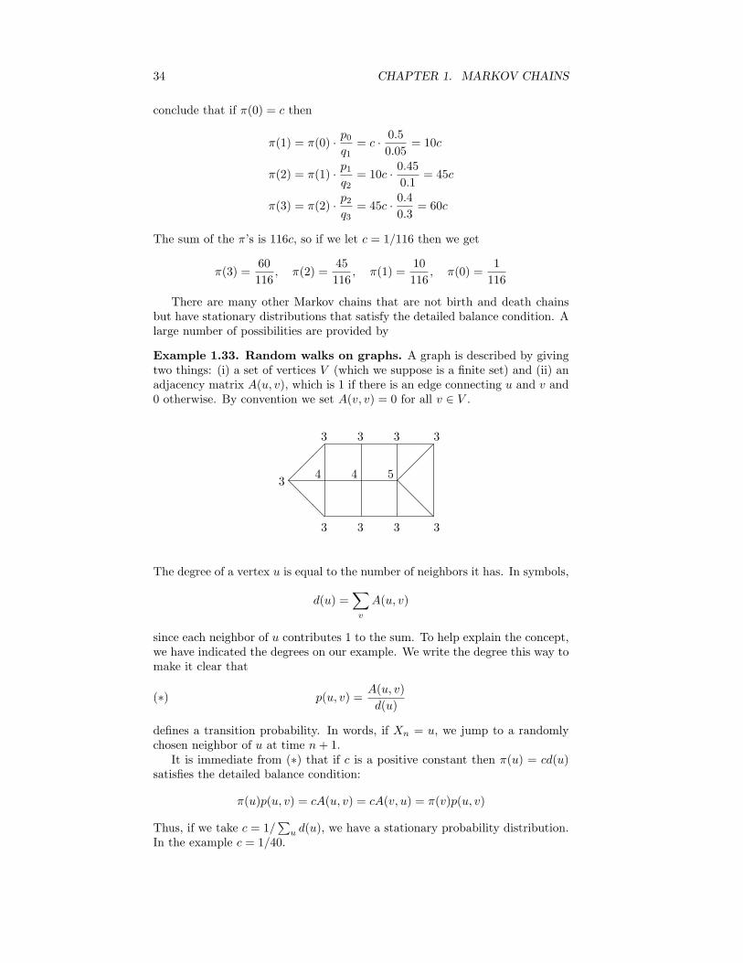
Example 1.33. Random walks on graphs. A graph is described by givingtwo things: (i) a set of vertices V (which we suppose is a finite set) and (ii) anadjacency matrix A(u, v), which is 1 if there is an edge connecting u and v and0 otherwise. By convention we set A(v, v) = 0 for all v ∈ V .
@@@
@@@
3 3 3 3
3 3 3 3
3 4 4 5
The degree of a vertex u is equal to the number of neighbors it has. In symbols,
d(u) =∑
v
A(u, v)
since each neighbor of u contributes 1 to the sum. To help explain the concept,we have indicated the degrees on our example. We write the degree this way tomake it clear that
(∗) p(u, v) =A(u, v)d(u)
defines a transition probability. In words, if Xn = u, we jump to a randomlychosen neighbor of u at time n + 1.
It is immediate from (∗) that if c is a positive constant then π(u) = cd(u)satisfies the detailed balance condition:
π(u)p(u, v) = cA(u, v) = cA(v, u) = π(v)p(u, v)
Thus, if we take c = 1/∑
u d(u), we have a stationary probability distribution.In the example c = 1/40.

1.6. SPECIAL EXAMPLES 35
For a concrete example, consider
Example 1.34. Random walk of a knight on a chess board. A chessboard is an 8 by 8 grid of squares. A knight moves by walking two steps in onedirection and then one step in a perpendicular direction.
×
• •
• •
••
••
By patiently examining all of the possibilities, one sees that the degrees ofthe vertices are given by the following table. Lines have been drawn to makethe symmetries more apparent.
2 3 4 4 4 4 3 23 4 6 6 6 6 4 34 6 8 8 8 8 6 44 6 8 8 8 8 6 44 6 8 8 8 8 6 44 6 8 8 8 8 6 43 4 6 6 6 6 4 32 3 4 4 4 4 3 2
The sum of the degrees is 4 · 2 + 8 · 3 + 20 · 4 + 16 · 6 + 16 · 8 = 336, so thestationary probabilities are the degrees divided by 336.
This problem is boring for a rook which has 14 possible moves from anysquare and hence a uniform stationary distribution. In exercises at the end ofthe chapter, we will consider the other three interesting examples: king, bishop,and queen.
1.6.3 Reversibility
Let p(i, j) be a transition probability with stationary distribution π(i). Let Xn
be a realization of the Markov chain starting from the stationary distribution,i.e., P (X0 = i) = π(i). The next result says that if we watch the process Xm,0 ≤ m ≤ n, backwards, then it is a Markov chain.

36 CHAPTER 1. MARKOV CHAINS
Theorem 1.25. Fix n and let Ym = Xn−m for 0 ≤ m ≤ n. Then Ym is aMarkov chain with transition probability
p(i, j) = P (Ym+1 = j|Ym = i) =π(j)p(j, i)
π(i)(1.13)
Proof. We need to calculate the conditional probability.
P (Ym+1 = im+1|Ym = im, Ym−1 = im−1 . . . Y0 = i0)
=P (Xn−(m+1) = im+1, Xn−m = im, Xn−m+1 = im−1 . . . Xn = i0)
P (Xn−m = im, Xn−m+1 = im−1 . . . Xn = i0)
Using the Markov property, we see the numerator is equal to
π(im+1)p(im+1, im)P (Xn−m+1 = im−1, . . . Xn = i0|Xn−m = im)
Similarly the denominator can be written as
π(im)P (Xn−m+1 = im−1, . . . Xn = i0|Xn−m = im)
Dividing the last two formulas and noticing that the conditional probabilitiescancel we have
P (Ym+1 = im+1|Ym = im, . . . Y0 = i0) =π(im+1)p(im+1, im)
π(im)
This shows Ym is a Markov chain with the indicated transition probability.
The formula for the transition probability in (1.13), which is called the dualtransition probability, may look a little strange, but it is easy to see that itworks; i.e., the p(i, j) ≥ 0, and have∑
j
p(i, j) =∑
j
π(j)p(j, i)π(i) =π(i)π(i)
= 1
since πp = π. When π satisfies the detailed balance conditions:
π(i)p(i, j) = π(j)p(j, i)
the transition probability for the reversed chain,
p(i, j) =π(j)p(j, i)
π(i)= p(i, j)
is the same as the original chain. In words, if we make a movie of the Markovchain Xm, 0 ≤ m ≤ n starting from an initial distribution that satisfies thedetailed balance condition and watch it backwards (i.e., consider Ym = Xn−m
for 0 ≤ m ≤ n), then we see a random process with the same distribution. m.To help explain the concept,
1.6.4 The Metropolis-Hastings algorithm
Our next topic is a method for generating samples from a distribution π(x). Itis named for two of the authors of the fundamental papers on the topic. One

1.6. SPECIAL EXAMPLES 37
written by Nicholas Metropolis and two married couples with last names Rosen-bluth and Teller (1953) and the other by W.K. Hastings (1970). This a veryuseful tool for computing posterior distributons in Bayesian statistics (Tierney(1994)), reconstructing images (Geman and Geman (1984)), and investigatingcomplicated models in statistical physics (Hammersley and Handscomb (1964)).It would take us too far afield to describe these applications, so we will contentourselves to describe the simple idea that is the key to the method.
We begin with a Markov chain q(x, y) that is the proposed jump distribution.A move is accepted with probability
r(x, y) = min
π(y)q(y, x)π(x)q(x, y)
, 1
so the transition probability
p(x, y) = q(x, y)r(x, y)
To check that π satisfies the detailed balance condition we can suppose thatπ(y)q(y, x) > π(x)q(x, y). In this case
π(x)p(x, y) = π(x)q(x, y) · 1
π(y)p(y, x) = π(y)q(y, x)π(x)q(x, y)π(y)q(y, x)
= π(x)q(x, y)
To generate one sample from π(x) we run the chain for a long time so thatit reaches equilibrium. To obtain many samples, we output the state at widelyseparated times. Of course there is an art of knowing how long is long enoughto wait between outputting the state to have independent realizations. If weare interested in the expected value of a particular function then (if the chainis irreducible and the state space is finite) Theorem 1.23 guarantees that
1n
n∑m=1
f(Xm)→∑
x
f(x)π(x)
The Metropolis-Hastings algorithm is often used when space is continuous,but that requires a more sophisticated Markov chain theory, so we will usediscrete examples to illustrate the method.
Example 1.35. Geometric distribution. Suppose π(x) = θx(1− θ) for x =0, 1, 2, . . .. To generate the jumps we will use a symmetric random walk q(x, x+1) = q(x, x − 1) = 1/2. Since q is symmetric r(x, y) = min1, π(y)/π(x). Inthis case if x > 0, π(x− 1) > π(x) and π(x + 1)/π(x) = θ so
p(x, x− 1) = 1/2 p(x, x + 1) = θ/2 p(x, x) = (1− θ)/2.
When x = 0, π(−1) = 0 so
p(0,−1) = 0 p(0, 1) = θ/2 p(0, 0) = 1− (θ/2).
To check reversibility we note that if x ≥ 0 then
π(x)p(x, x + 1) = θx(1− θ) · θ2
= π(x + 1)p(x + 1, x)
Here, as in most applications of the Metropolis-Hastings algorithm the choiceof q is important. If θ is close to 1 then we would want to choose q(x, x + i) =1/2L + 1 for −L ≤ i ≤ L where L = O(1/(1 − θ)) to make the chain movearound the state space faster while not having too many steps rejected.

38 CHAPTER 1. MARKOV CHAINS
Example 1.36. Binomial distribution. Suppose π(x) is Binomial(N, θ).In this case we can let q(x, y) = 1/(N + 1) for all 0 ≤ x, y ≤ N . Sinceq is symmetric r(x, y) = min1, π(y)/π(x). This is closely related to themethod of rejection sampling, in which one generates independent randomvariables Ui uniform on 0, 1, . . . , N and keep Ui with probability π(Ui)/π∗
where π∗ = max0≤x≤n π(x).
Example 1.37. Two dimensional Ising model. The Metropolis-Hastingsalgorithm has its roots in statistical physics. A typical problem is the Isingmodel of ferromagnetism. Space is represented by a two dimensional grid Λ =−L, . . . L2. If we made the lattice three dimensional, we could think of theatoms in an iron bar. In reality each atom has a spin which can point in somedirection, but we simplify by supposing that each spin can be up +1 or down−1. The state of the systems is a function ξ : Λ → −1, 1 i.e., a point in theproduct space −1, 1Λ. We say that points x and y in Λ are neighbors if y isone of the four points x + (1, 0), x + (−1, 0), x + (0, 1), x + (0,−1). See thepicture:
+ − + + + − −− − − + + + −+ − + + − − ++ + − − y + −+ − + y x y −− − − + y + −+ − + + − − +
Given an interaction parameter β, which is inversely proportional to the tem-perature, the equilibrium state is
π(x) =1
Z(β)exp
(β∑
x,y∼x
ξxξy
)
where the sum is over all x, y ∈ Λ with y a neighbor of x, and Z(β) is a constantthat makes the probabilities sum to one. At the boundaries of the square spinshave only three neighbors. There are several options for dealing with this: (i)we consider the spins outside to be 0, or (ii) we could specify a fixed boundarycondition such as all spins +.
The sum is largest in case (i) when all of the spins agree or in case (ii) whenall spins are +. These configuration minimizes the energy H = −
∑x,y∼x ηxηy
but there many more configurations one with a random mixture of +’s and −’s.It turns out that as β increases the system undergoes a phase transition froma random state with an almost equal number of +’s and −’s to one in whichmore than 1/2 of the spins point in the same direction.
Z(β) is difficult to compute so it is fortunate that only the ratio of theprobabilities appears in the Metropolis-Hastings recipe. For the proposed jumpdistribution we let q(ξ, ξx) = 1/(2L + 1)2 if the two configurations ξ and ξx
differ only at x. In this case the transition probability is
p(ξ, ξx) = q(ξ, ξx) min
π(ξx)π(ξ)
, 1
Note that the ratio π(ξx)/π(ξ) is easy to compute because Z(β) cancels out,as do all the terms in the sum that do not involve x and its neighbors. Since

1.7. PROOFS OF THE MAIN THEOREMS* 39
ξx(x) = −ξ(x).π(ξx)π(ξ)
= exp
(−2β
∑y∼x
ξxξy
)If x agrees with k of its four neighbors the ratio is exp(−2(4 − 2k)). In wordsp(x, y) can be described by saying that we accept the proposed move withprobability 1 if it lowers the energy and with probability π(y)/π(x) if not.
Example 1.38. Simulated annealing. The Metropolis-Hastings algorithmcan also be used to minimize complicated functions. Consider for example thetraveling salesman problem, which is to find the shortest (or least expensive)route that allows one to visit all of the cities on a list. In this case the statespace will be lists of cities, x and π(x) = exp(−β`(x)) where `(x) is the lengthof the tour. The proposal kernel q is chosen to modify the list in some way.For example, we might move a city to a another place on the list or reversethe order of a sequence of cities. When β is large the stationary distributionwill concentrate on optimal and near optimal tours. As in the Ising model, βis thought of as inverse temperature. The name derives from the fact that toforce the chain to better solution we increase β (i.e., reduce the temperature)as we run the simulation. One must do this slowly or the process will get stuckin local minima. For more of simulated annealing see Kirkpatrick et al. (1983)
1.7 Proofs of the Main Theorems*
To prepare for the proof of the convergence theorem, Theorem 1.19, we needthe following:
Lemma 1.26. If there is a stationary distribution, then all states y that haveπ(y) > 0 are recurrent.
Proof. Lemma 1.12 tells us that ExN(y) =∑∞
n=1 pn(x, y), so
∑x
π(x)ExN(y) =∑
x
π(x)∞∑
n=1
pn(x, y)
Interchanging the order of summation and then using πpn = π, the above
=∞∑
n=1
∑x
π(x)pn(x, y) =∞∑
n=1
π(y) =∞
since π(y) > 0. Using Lemma 1.11 now gives ExN(y) = ρxy/(1− ρyy), so
∞ =∑
x
π(x)ρxy
1− ρyy≤ 1
1− ρyy
the second inequality following from the facts that ρxy ≤ 1 and π is a probabilitymeasure. This shows that ρyy = 1, i.e., y is recurrent.
With Lemma 1.26 in hand we are ready to tackle the proof of:
Theorem 1.19. Convergence theorem. Suppose p is irreducible, aperiodic,and has stationary distribution π. Then as n→∞, pn(x, y)→ π(y).

40 CHAPTER 1. MARKOV CHAINS
Proof. Let S be the state space for p. Define a transition probability p on S×Sby
p((x1, y1), (x2, y2)) = p(x1, x2)p(y1, y2)
In words, each coordinate moves independently.
Step 1. We will first show that if p is aperiodic and irreducible then p isirreducible. Since p is irreducible, there are K, L, so that pK(x1, x2) > 0 andpL(y1, y2) > 0. Since x2 and y2 have period 1, it follows from Lemma 1.16 thatif M is large, then pL+M (x2, x2) > 0 and pK+M (y2, y2) > 0, so
pK+L+M ((x1, y1), (x2, y2)) > 0
Step 2. Since the two coordinates are independent π(a, b) = π(a)π(b) definesa stationary distribution for p, and Lemma 1.26 implies that all states arerecurrent for p. Let (Xn, Yn) denote the chain on S × S, and let T be the firsttime that the two coordinates are equal, i.e., T = minn ≥ 0 : Xn = Yn. LetV(x,x) = minn ≥ 0 : Xn = Yn = x be the time of the first visit to (x, x).Since p is irreducible and recurrent, V(x,x) < ∞ with probability one. SinceT ≤ V(x,x) for any x we must have
P (T <∞) = 1. (1.14)
Step 3. By considering the time and place of the first intersection and thenusing the Markov property we have
P (Xn = y, T ≤ n) =n∑
m=1
∑x
P (T = m,Xm = x,Xn = y)
=n∑
m=1
∑x
P (T = m,Xm = x)P (Xn = y|Xm = x)
=n∑
m=1
∑x
P (T = m,Ym = x)P (Yn = y|Ym = x)
= P (Yn = y, T ≤ n)
Step 4. To finish up we observe that since the distributions of Xn and Yn
agree on T ≤ n
|P (Xn = y)− P (Yn = y)| ≤ P (Xn = y, T > n) + P (Yn = y, T > n)
and summing over y gives∑y
|P (Xn = y)− P (Yn = y)| ≤ 2P (T > n)
If we let X0 = x and let Y0 have the stationary distribution π, then Yn hasdistribution π, and Using (1.14) it follows that∑
y
|pn(x, y)− π(y)| ≤ 2P (T > n)→ 0
proving the convergence theorem.

1.7. PROOFS OF THE MAIN THEOREMS* 41
Our next topic is the existence of stationary measures
Theorem 1.20. Suppose p is irreducible and recurrent. Let x ∈ S and letTx = infn ≥ 1 : Xn = x.
µx(y) =∞∑
n=0
Px(Xn = y, Tx > n)
defines a stationary measure with 0 < µx(y) <∞ for all y.
Why is this true? This is called the “cycle trick.” µx(y) is the expectednumber of visits to y in 0, . . . , Tx − 1. Multiplying by p moves us forwardone unit in time so µxp(y) is the expected number of visits to y in 1, . . . , Tx.Since X(Tx) = X0 = x it follows that µx = µxp.
AAAA@@AAAA@@•
•
•
•
•
•
•
•
x
y
0 Tx
Figure 1.2: Picture of the cycle trick.
Proof. To formalize this intuition, let pn(x, y) = Px(Xn = y, Tx > n) andinterchange sums to get∑
y
µx(y)p(y, z) =∞∑
n=0
∑y
pn(x, y)p(y, z)
Case 1. Consider the generic case first: z 6= x.∑y
pn(x, y)p(y, z) =∑
y
Px(Xn = y, Tx > n,Xn+1 = z)
= Px(Tx > n + 1, Xn+1 = z) = pn+1(x, z)
Here the second equality holds since the chain must be somewhere at time n,and the third is just the definition of pn+1. Summing from n = 0 to∞, we have
∞∑n=0
∑y
pn(x, y)p(y, z) =∞∑
n=0
pn+1(x, z) = µx(z)
since p0(x, z) = 0.
Case 2. Now suppose that z = x. Reasoning as above we have∑y
pn(x, y)p(y, x) =∑
y
Px(Xn = y, Tx > n,Xn+1 = x) = Px(Tx = n + 1)
42 CHAPTER 1. MARKOV CHAINS
Summing from n = 0 to ∞ we have∞∑
n=0
∑y
pn(x, y)p(y, x) =∞∑
n=0
Px(Tx = n + 1) = 1 = µx(x)
since Px(Tx = 0) = 0.To check µx(y) <∞, we note that µx(x) = 1 and
1 = µx(x) =∑
z
µx(z)pn(z, x) ≥ µx(y)pn(y, x)
so if we pick n with pn(y, x) > 0 then we conclude µx(y) <∞.To prove that µx(y) > 0 we note that this is trivial for y = x the point
used to define the measure. For y 6= x, we borrow an idea from Theorem 1.5.Let K = mink : pk(x, y) > 0. Since pK(x, y) > 0 there must be a sequencey1, . . . yK−1 so that
p(x, y1)p(y1, y2) · · · p(yK−1, y) > 0
Since K is minimal all the yi 6= y, so Px(XK = y, Tx > K) > 0 and henceµx(y) > 0.
Our next step is to prove
Theorem 1.21. Suppose p is irreducible and recurrent. Let Nn(y) be thenumber of visits to y at times ≤ n. As n→∞
Nn(y)n
→ 1EyTy
Why is this true? Suppose first that we start at y. The times between returns,t1, t2, . . . are independent and identically distributed so the strong law of largenumbers for nonnegative random variables implies that the time of the kthreturn to y, R(k) = minn ≥ 1 : Nn(y) = k, has
R(k)k→ EyTy ≤ ∞ (1.15)
If we do not start at y then t1 <∞ and t2, t3, . . . are independent and identicallydistributed and we again have (1.15). Writing ak ∼ bk when ak/bk → 1 we haveR(k) ∼ kEyTy. Taking k = n/EyTy we see that there are about n/EyTy returnsby time n.
Proof. We have already shown (1.15). To turn this into the desired result, wenote that from the definition of R(k) it follows that R(Nn(y)) ≤ n < R(Nn(y)+1). Dividing everything by Nn(y) and then multiplying and dividing on the endby Nn(y) + 1, we have
R(Nn(y))Nn(y)
≤ n
Nn(y)<
R(Nn(y) + 1)Nn(y) + 1
· Nn(y) + 1Nn(y)
Letting n→∞, we have n/Nn(y) trapped between two things that converge toEyTy, so
n
Nn(y)→ EyTy
and we have proved the desired result.

1.7. PROOFS OF THE MAIN THEOREMS* 43
Theorem 1.22. If p is an irreducible and has stationary distribution π, then
π(y) = 1/EyTy
Proof. Suppose X0 has distribution π. From Theorem 1.21 it follows that
Nn(y)n
→ 1EyTy
Taking expected value and using the fact that Nn(y) ≤ n, it can be shown thatthis implies
EπNn(y)n
→ 1EyTy
but since π is a stationary distribution EπNn(y) = nπ(y).
Theorem 1.23. Suppose p is irreducible, has stationary distribution π, and∑x |f(x)|π(x) <∞ then
1n
n∑m=1
f(Xm)→∑
x
f(x)π(x)
The key idea here is that by breaking the path at the return times to x we get aseqeunce of random variables to which we can apply the law of large numbers.
Sketch of proof. Suppose that the chain starts at x. Let T0 = 0 and Tk =minn > Tk−1 : Xn = x be the time of the kth return to x. By the strongMarkov property, the random variables
Yk =Tk∑
m=Tk−1+1
f(Xm)
are independent and identically distributed. By the cycle trick in the proof ofTheorem 1.20
EYk =∑
x
µx(y)f(y)
Using the law of large numbers for i.i.d. variables
1L
TL∑m=1
f(Xm) =1L
L∑k=1
Yk →∑
x
µx(y)f(y)
Taking L = Nn(x) = maxk : Tk ≤ n and ignoring the contribution from thelast incomplete cycle (Nn(x), n]
1n
n∑m=1
f(Xm) ≈ Nn(x)n· 1Nn(x)
Nn(x)∑k=1
Yk
Using Theorem 1.21 and the law of large numbers the above
→ 1ExTx
∑y
µx(y)f(y) =∑
y
π(y)f(y)
44 CHAPTER 1. MARKOV CHAINS
1.8 Exit Distributions
To motivate developments, we begin with an example.
Example 1.39. Two year college. At a local two year college, 60% of fresh-men become sophomores, 25% remain freshmen, and 15% drop out. 70% ofsophomores graduate and transfer to a four year college, 20% remain sopho-mores and 10% drop out. What fraction of new students eventually graduate?
We use a Markov chain with state space 1 = freshman, 2 = sophomore, G= graduate, D = dropout. The transition probability is
1 2 G D1 0.25 0.6 0 0.152 0 0.2 0.7 0.1G 0 0 1 0D 0 0 0 1
Let h(x) be the probability that a student currently in state x eventually grad-uates. By considering what happens on one step
h(1) = 0.25h(1) + 0.6h(2)h(2) = 0.2h(2) + 0.7
To solve we note that the second equation implies h(2) = 7/8 and then the firstthat
h(1) =0.60.75
· 78
= 0.7
Example 1.40. Tennis. In tennis the winner of a game is the first player towin four points, unless the score is 4− 3, in which case the game must continueuntil one player is ahead by two points and wins the game. Suppose that theserver win the point with probability 0.6 and successive points are independent.What is the probability the server will win the game if the score is tied 3-3? ifshe is ahead by one point? Behind by one point?
We formulate the game as a Markov chain in which the state is the differenceof the scores. The state space is 2, 1, 0,−1,−2 with 2 (win for server) and −2(win for opponent). The transition probability is
2 1 0 -1 -22 1 0 0 0 01 .6 0 .4 0 00 0 .6 0 .4 0
-1 0 0 .6 0 .4-2 0 0 0 0 1
If we let h(x) be the probability of the server winning when the score is x then
h(x) =∑
y
p(x, y)h(y)
with h(2) = 1 and h(−2) = 0. This gives us three equations in three unknowns
h(1) = .6 + .4h(0)h(0) = .6h(1) + .4h(−1)
h(−1) = .6h(0)

1.8. EXIT DISTRIBUTIONS 45
Using the first and third equations in the second we have
h(0) = .6(.6 + .4h(0)) + .4(.6h(0)) = .36 + .48h(0)
so we have h(0) = 0.36/0.52 = 0.6923.The last computation uses special properties of this example. To introduce
a general approach, we rearrange the equations to get
h(1)− .4h(0) + 0h(−1) = .6−.6h(1) + h(0)− .4h(−1) = 0
0h(1)− .6h(0) + h(−1) = 0
which can be written in matrix form as 1 −.4 0−.6 1 −.40 −.6 1
h(1)h(0)
h(−1)
=
.600
Let C = 1, 0,−1 be the nonabsorbing states and let r(x, y) the restrictionof p to x, y ∈ C (i.e., the 3 × 3 matrix inside the black lines in the transitionprobability). In this notation then the matrix above is I − r. Solving gives h(1)
h(0)h(−1)
= (I − r)−1
.600
=
.8769.6923.4154
General solution. Suppose that the server wins each point with prob-
ability w. If the game is tied then after two points, the server will havewon with probability w2, lost with probability (1 − w)2, and returned to atied game with probability 2w(1 − w), so h(0) = w2 + 2w(1 − w)h(0). Since1− 2w(1− w) = w2 + (1− w)2, solving gives
h(0) =w2
w2 + (1− w)2
Figure 1.3 graphs this function.Having worked two examples, it is time to show that we have computed the
right answer. In some cases we will want to guess and verify the answer. Inthose situations it is nice to know that the solution is unique. The next resultproves this.
Theorem 1.27. Consider a Markov chain with finite state space S. Let a andb be two points in S, and let C = S − a, b. Suppose h(a) = 1, h(b) = 0, andthat for x ∈ C we have
h(x) =∑
y
p(x, y)h(y) (1.16)
If Px(Va ∧ Vb <∞) > 0 for all x ∈ C, then h(x) = Px(Va < Vb).
Proof. Let T = Va ∧ Vb. It follows from Lemma 1.3 that Px(T < ∞) = 1 forall x ∈ C. (1.16) implies that h(x) = Exh(X1) when x 6= a, b. The Markovproperty implies
h(x) = Exh(XT∧n).
We have to stop at time T because the equation is not assumed to be valid forx = a, b. Since S is finite, Px(T <∞) = 1 for all x ∈ C, h(a) = 1, and h(b) = 0,it is not hard to prove that Exh(XT∧n)→ Px(Va < Vb) which gives the desiredresult.

46 CHAPTER 1. MARKOV CHAINS
0.5
0.6
0.7
0.8
0.9
1
0.5 0.6 0.7 0.8 0.9 1
Figure 1.3: Probability the server winning a tied game as a function of theprobability of winning a point.
Example 1.41. Matching pennies. Bob, who has 15 pennies, and Charlie,who has 10 pennies, decide to play a game. They each flip a coin. If the twocoins match, Bob gets the two pennies (for a profit of 1). If the two coins aredifferent, then Charlie gets the two pennies. They quit when someone has allof the pennies. What is the probability Bob will win the game?
The answer will turn out to be 15/25, Bob’s fraction of the total supply ofpennies. To explain this, let Xn be the number of pennies Bob has after nplays. Xn is a fair game, i.e., x = ExX1, or in words the expected number ofpennies Bob has is constant in time. Let
Vy = minn ≥ 0 : Xn = y
be the time of the first visit to y. Taking a leap of faith the expected numberhe has at the end of the game should be the same as at the beginning so
x = NPx(VN < V0) + 0Px(V0 < Vn)
and solving gives
Px(VN < V0) = x/N for 0 ≤ x ≤ N (1.17)
To prove this note that by considering what happens on the first step
h(x) =12h(x + 1) +
12h(x− 1)
Multiplying by 2 and rearranging
h(x + 1)− h(x) = h(x)− h(x− 1)
or in words, h has constant slope. Since h(0) = 0 and h(N) = 1 the slope mustbe 1/N and we must have h(x) = x/N .
The reasoning in the last example can be used to study Example 1.9.

1.8. EXIT DISTRIBUTIONS 47
Example 1.42. Wright–Fisher model with no mutation. The state spaceis S = 0, 1, . . . N and the transition probability is
p(x, y) =N
y
( x
N
)y(
N − x
N
)N−y
The right-hand side is the binomial(N,x/N) distribution, i.e., the number ofsuccesses in N trials when success has probability x/N , so the mean number ofsuccesses is x. From this it follows that if we define h(x) = x/N , then
h(x) =∑
y
p(x, y)h(y)
Taking a = N and b = 0, we have h(a) = 1 and h(b) = 0. Since Px(Va ∧ Vb <∞) > 0 for all 0 < x < N , it follows from Lemma 1.27 that
Px(VN < V0) = x/N (1.18)
i.e., the probability of fixation to all A’s is equal to the fraction of the genesthat are A.
Our next topic is non-fair games.
Example 1.43. Gambler’s ruin. Consider a gambling game in which onany turn you win $1 with probability p 6= 1/2 or lose $1 with probability 1− p.Suppose further that you will quit playing if your fortune reaches $N . Of course,if your fortune reaches $0, then the casino makes you stop. Let
h(x) = Px(VN < V0)
be the happy event that our gambler reaches the goal of $N before goingbankrupt when starting with $x. Thanks to our definition of Vx as the mini-mum of n ≥ 0 with Xn = x we have h(0) = 0, and h(N) = 1. To calculate h(x)for 0 < x < N , we set q = 1 − p to simplify the formulas, and consider whathappens on the first step to arrive at
h(x) = ph(x + 1) + qh(x− 1) (1.19)
To solve this we rearrange to get p(h(x + 1)− h(x)) = q(h(x)− h(x− 1)) andconclude
h(x + 1)− h(x) =q
p· (h(x)− h(x− 1)) (1.20)
If we set c = h(1)− h(0) then (1.20) implies that for x ≥ 1
h(x)− h(x− 1) = c
(q
p
)x−1
Summing from x = 1 to N , we have
1 = h(N)− h(0) =N∑
x=1
h(x)− h(x− 1) = c
N∑x=1
(q
p
)x−1
Now for θ 6= 1 the partial sum of the geometric series is
N−1∑j=0
θj =1− θN
1− θ(1.21)

48 CHAPTER 1. MARKOV CHAINS
To check this note that
(1− θ)(1 + θ + · · · θN−1) = (1 + θ + · · · θN−1)
− (θ + θ2 + · · · θN ) = 1− θN
Using (1.21) we see that c = (1 − θ)/(1 − θN ) with θ = q/p. Summing andusing the fact that h(0) = 0, we have
h(x) = h(x)− h(0) = c
x−1∑i=0
θi = c · 1− θx
1− θ=
1− θx
1− θN
Recalling the definition of h(x) and rearranging the fraction we have
Px(VN < V0) =θx − 1θN − 1
where θ = 1−pp (1.22)
To see what (1.22) says in a concrete example, we consider:
Example 1.44. Roulette. If we bet $1 on red on a roulette wheel with 18red, 18 black, and 2 green (0 and 00) holes, we win $1 with probability 18/38 =0.4737 and lose $1 with probability 20/38. Suppose we bring $50 to the casinowith the hope of reaching $100 before going bankrupt. What is the probabilitywe will succeed?
Here θ = q/p = 20/18, so (1.22) implies
P50(V100 < V0) =
(2018
)50 − 1(2018
)100 − 1
Using (20/18)50 = 194, we have
P50(V100 < V0) =194− 1
(194)2 − 1=
1194 + 1
= 0.005128
Now let’s turn things around and look at the game from the viewpoint of thecasino, i.e., p = 20/38. Suppose that the casino starts with the rather modestcapital of x = 100. (1.22) implies that the probability they will reach N beforegoing bankrupt is
(9/10)100 − 1(9/10)N − 1
If we let N →∞, (9/10)N → 0 so the answer converges to
1− (9/10)100 = 1− 2.656× 10⁻⁵
If we increase the capital to $200 then the failure probability is squared, since tobecome bankrupt we must first lose $100 and then lose our second $100. In thiscase the failure probability is incredibly small: (2.656×10⁻⁵)2 = 7.055×10⁻¹⁰.
From the last analysis we see that if p > 1/2, q/p < 1 and letting N → ∞in (1.22) gives
Px(V0 =∞) = 1−(
q
p
)x
and Px(V0 <∞) =(
q
p
)x
. (1.23)
To see that the form of the last answer makes sense, note that to get from x to0 we must go x→ x− 1→ x2 . . .→ 1→ 0, so
Px(V0 <∞) = P1(V0 <∞)x.

1.9. EXIT TIMES 49
1.9 Exit Times
To motivate developments we begin with an example.
Example 1.45. Two year college. In Example 1.39 we introduced a Markovchain with state space 1 = freshman, 2 = sophomore, G = graduate, D =dropout, and transition probability
1 2 G D1 0.25 0.6 0 0.152 0 0.2 0.7 0.1G 0 0 1 0D 0 0 0 1
On the average how many years does a student take to graduate or drop out?
Let g(x) be the expected time for a student starting in state x. g(G) =g(D) = 0. By considering what happens on one step
g(1) = 1 + 0.25g(1) + 0.6g(2)g(2) = 1 + 0.2g(2)
where the 1+ is due to the fact that after the jump has been made one yearhas elapsed. To solve for g, we note that the second equation implies g(2) =1/0.8 = 1.25 and then the first that
g(1) =1 + 0.6(1.25)
0.75=
1.750.75
= 2.3333
Example 1.46. Tennis. In Example 1.40 we formulated the last portion ofthe game as a Markov chain in which the state is the difference of the scores.The state space was S = 2, 1, 0,−1,−2 with 2 (win for server) and −2 (winfor opponent). The transition probability was
2 1 0 -1 -22 1 0 0 0 01 .6 0 .4 0 00 0 .6 0 .4 0
-1 0 0 .6 0 .4-2 0 0 0 0 1
Let g(x) be the expected time to complete the game when the current stateis x. By considering what happens on one step
g(x) = 1 +∑
y
p(x, y)g(y)
Since g(2) = g(−2) = 0, if we let r(x, y) be the restriction of the transitionprobability to 1, 0,−1 we have
g(x)−∑
y
r(x, y)g(y) = 1
Writing 1 for a 3× 1 matrix (i.e., column vector) with all 1’s we can write thisas
(I − r)g = 1

50 CHAPTER 1. MARKOV CHAINS
so g = (I − r)−11.There is another way to see this. If N(y) is the number of visits to y at
times n ≥ 0, then from (1.12)
ExN(y) =∞∑
n=0
rn(x, y)
To see that this is (I − r)−1(x, y) note that (I − r)(I + r + r2 + r3 + · · · )
= (I + r + r2 + r3 + · · · )− (r + r2 + r3 + r4 · · · ) = I
If T is the duration of the game then T =∑
y N(y) so
ExT = (I − r)−11 (1.24)
To solve the problem now we note that
I − r =
1 −.4 0−.6 1 −.40 −.6 1
(I − r)−1 =
19/13 10/13 4/1315/13 25/13 10/139/13 15/13 19/13
so E0T = (15 + 25 + 10)/13 = 50/13 = 3.846 points. Here the three terms inthe sum are the expected number of visits to −1, 0, and 1.
Having worked two examples, it is time to show that we have computed theright answer. In some cases we will want to guess and verify the answer. Inthose situations it is nice to know that the solution is unique. The next resultproves this.
Theorem 1.28. Consider a Markov chain with finite state space S. Let A ⊂ Sand VA = infn ≥ 0 : Xn ∈ A. We suppose C = S − A is finite, and thatPx(VA < ∞) > 0 for any x ∈ C. Suppose g(a) = 0 for all a ∈ A, and that forx ∈ C we have
g(x) = 1 +∑
y
p(x, y)g(y) (1.25)
Then g(x) = Ex(VA).
Proof. It follows from Lemma 1.3 that ExVA <∞ for all x ∈ C. (1.25) impliesthat g(x) = 1 + Exg(X1) when x 6∈ A. The Markov property implies
g(x) = Ex(T ∧ n) + Exg(XT∧nn).
We have to stop at time T because the equation is not valid for x ∈ A. Itfollows from the definition of the expected value that Ex(T ∧ n) ↑ ExT . SinceS is finite, Px(T < ∞) = 1 for all x ∈ C, g(a) = 0 for a ∈ A, it is not hard tosee that Exg(XT∧n)→ 0.
Example 1.47. Waiting time for TT. Let TTT be the (random) numberof times we need to flip a coin before we have gotten Tails on two consecutivetosses. To compute the expected value of TTT we will introduce a Markov chainwith states 0, 1, 2 = the number of Tails we have in a row.

1.9. EXIT TIMES 51
Since getting a Tails increases the number of Tails we have in a row by 1, butgetting a Heads sets the number of Tails we have in a row to 0, the transitionmatrix is
0 1 20 1/2 1/2 01 1/2 0 1/22 0 0 1
Since we are not interested in what happens after we reach 2 we have made 2an absorbing state. If we let V2 = minn ≥ 0 : Xn = 2 and g(x) = ExV2 thenone step reasoning gives
g(0) = 1 + .5g(0) + .5g(1)g(1) = 1 + .5g(0)
Plugging the second equation into the first gives g(0) = 1.5 + .75g(0), so.25g(0) = 1.5 or g(0) = 6. To do this with the previous approach we note
I − r =(
1/2 −1/2−1/2 1
)(I − r)−1 =
(4 22 2
)so E0V2 = 6.
Example 1.48. Waiting time for HT. Let THT be the (random) number oftimes we need to flip a coin before we have gotten a Heads followed by a Tails.Consider Xn is Markov chain with transition probability:
HH HT TH TTHH 1/2 1/2 0 0HT 0 0 1/2 1/2TH 1/2 1/2 0 0TT 0 0 1/2 1/2
If we eliminate the row and the column for HT then
I − r =
1/2 0 0−1/2 1 0
0 −1/2 1/2
(I − r)−11 =
224
To compute the expected waiting time for our original problem, we note thatafter the first two tosses we have each of the four possibilities with probability1/4 so
ETHT = 2 +14(0 + 2 + 2 + 4) = 4
Why is ETTT = 6 while ETHT = 4? To explain we begin by noting thatEyTy = 1/π(y) and the stationary distribution assigns probability 1/4 to eachstate. One can verify this and check that convergence to equilibrium is rapidby noting that all the entries of p2 are equal to 1/4. Our identity implies that
EHT THT =1
π(HT )= 4
To get from this to what we wanted to calculate, note that if we start with aH at time −1 and a T at time 0, then we have nothing that will help us in the
52 CHAPTER 1. MARKOV CHAINS
future, so the expected waiting time for a HT when we start with nothing isthe same.
When we consider TT , our identity again gives
ETT TTT =1
π(TT )= 4
However, this time if we start with a T at time −1 and a T at time 0, then aT at time 1 will give us a TT and a return to TT at time 1; while if we get aH at time 1, then we have wasted 1 turn and we have nothing that can help uslater, so
4 = ETT TTT =12· 1 +
12· (1 + ETTT )
Solving gives ETTT = 6, so it takes longer to observe TT . The reason for this,which can be seen in the last equation, is that once we have one TT , we willget another one with probability 1/2, while occurrences of HT cannot overlap.
In the Exercise 1.59 we will consider waiting times for three coin patterns.The most interesting of these is ETHTH = ETTHT .
Example 1.49. Duration of fair games. Consider the gambler’s ruin chainin which p(i, i + 1) = p(i, i − 1) = 1/2. Let τ = minn : Xn 6∈ (0, N). Weclaim that
Exτ = x(N − x) (1.26)
To see what formula (1.26) says, consider matching pennies. There N = 25 andx = 15, so the game will take 15 · 10 = 150 flips on the average. If there aretwice as many coins, N = 50 and x = 30, then the game takes 30 · 20 = 600flips on the average, or four times as long.
There are two ways to prove this.
Verify the guess. Let g(x) = x(N −x). Clearly, g(0) = g(N) = 0. If 0 < x < Nthen by considering what happens on the first step we have
g(x) = 1 +12g(x + 1) +
12g(x− 1)
If g(x) = x(N − x) then the right-hand side is
= 1 +12(x + 1)(N − x− 1) +
12(x− 1)(N − x + 1)
= 1 +12[x(N − x)− x + N − x− 1] +
12[x(N − x) + x− (N − x + 1)]
= 1 + x(N − x)− 1 = x(N − x)
Derive the answer. (1.25) implies that
g(x) = 1 + (1/2)g(x + 1) + (1/2)g(x− 1)
Rearranging gives
g(x + 1)− g(x) = −2 + g(x)− g(x− 1)
Setting g(1)− g(0) = c we have g(2)− g(1) = c− 2, g(3)− g(2) = c− 4 and ingeneral that
g(k)− g(k − 1) = c− 2(k − 1)

1.10. INFINITE STATE SPACES* 53
Using g(0) = 0 and summing we have
0 = g(N) =N∑
k=1
c− 2(k − 1) = cN − 2 · N(N − 1)2
since, as one can easily check by induction,∑m
j=1 j = m(m + 1)/2. Solvinggives c = (N − 1). Summing again, we see that
g(x) =x∑
k=1
(N − 1)− 2(k − 1) = x(N − 1)− x(x + 1) = x(N − x)
Example 1.50. Duration of nonfair games. Consider the gambler’s ruinchain in which p(i, i + 1)p and p(i, i − 1) = q, where p 6= q. Let τ = minn :Xn 6∈ (0, N). We claim that
Exτ =x
q − p− N
q − p· 1− (q/p)x
1− (q/p)N(1.27)
This time the derivation is somewhat tedious, so we will just verify the guess.We want to show that g(x) = 1 + pg(x + 1) + qg(x− 1). Plugging the formulainto the right-hand side:
=1 + px + 1q − p
+ qx− 1q − p
− N
q − p
[p · 1− (q/p)x+1
1− (q/p)N+ q
1− (q/p)x−1
1− (q/p)N
]=1 +
x
q − p+
p− q
q − p− N
q − p
[p + q − (q/p)x(q + p)
1− (q/p)N
]which = g(x) since p + q = 1.
To see what this says note that if p < q then q/p > 1 so
N
1− (q/p)N→ 0 and g(x) =
x
q − p(1.28)
To see this is reasonable note that our expected value on one play is p − q, sowe lose an average of q− p per play, and it should take an average of x/(q− p)to lose x dollars.
When p > q, (q/p)N → 0, so doing some algebra
g(x) ≈ N − x
p− q[1− (q/p)x] +
x
p− q(q/p)x
Using (1.23) we see that the probability of not hitting 0 is 1 − (q/p)x. Inthis case, since our expected winnings per play is p − q, it should take about(N −x)/(p− q) plays to get to N . The second term represents the contributionto the expected value from paths that end at 0, but it is hard to explain whythe term has exactly this form.
1.10 Infinite State Spaces*
In this section we consider chains with an infinite state space. The major newcomplication is that recurrence is not enough to guarantee the existence of astationary distribution.

54 CHAPTER 1. MARKOV CHAINS
Example 1.51. Reflecting random walk. Imagine a particle that moves on0, 1, 2, . . . according to the following rules. It takes a step to the right withprobability p. It attempts to take a step to the left with probability 1− p, butif it is at 0 and tries to jump to the left, it stays at 0, since there is no −1 tojump to. In symbols,
p(i, i + 1) = p when i ≥ 0p(i, i− 1) = 1− p when i ≥ 1
p(0, 0) = 1− p
This is a birth and death chain, so we can solve for the stationary distributionusing the detailed balance equations:
pπ(i) = (1− p)π(i + 1) when i ≥ 0
Rewriting this as π(i + 1) = π(i) · p/(1− p) and setting π(0) = c, we have
π(i) = c
(p
1− p
)i
(1.29)
There are now three cases to consider:
p < 1/2: p/(1− p) < 1. π(i) decreases exponentially fast, so∑
i π(i) <∞, andwe can pick c to make π a stationary distribution. To find the value of c tomake π a probability distribution we recall
∞∑i=0
θi = 1/(1− θ) when θ < 1.
Taking θ = p/(1− p) and hence 1− θ = (1− 2p)/(1− p), we see that the sumof the π(i) defined in (∗) is c(1− p)/(1− 2p), so
π(i) =1− 2p
1− p·(
p
1− p
)i
= (1− θ)θi (1.30)
To confirm that we have succeeded in making the π(i) add up to 1, note thatif we are flipping a coin with a probability θ of Heads, then the probability ofgetting i Heads before we get our first Tails is given by π(i).
The reflecting random walk is clearly irreducible. To check that it is aperi-odic note that p(0, 0) > 0 implies 0 has period 1, and then Lemma 1.18 impliesthat all states have period 1. Using the convergence theorem, Theorem 1.19,now we see that
I. When p < 1/2, P (Xn = j)→ π(j), the stationary distribution in (1.30).
Using Theorem 1.22 now,
E0T0 =1
π(0)=
11− θ
=1− p
1− 2p(1.31)
It should not be surprising that the system stabilizes when p < 1/2. Inthis case movements to the left have a higher probability than to the right, sothere is a drift back toward 0. On the other hand if steps to the right are more

1.10. INFINITE STATE SPACES* 55
frequent than those to the left, then the chain will drift to the right and wanderoff to ∞.
II. When p > 1/2 all states are transient.
(1.23) implies that if x > 0, Px(T0 <∞) = ((1− p)/p)x.
To figure out what happens in the borderline case p = 1/2, we use resultsfrom Sections 1.8 and 1.9. Recall we have defined Vy = minn ≥ 0 : Xn = yand (1.17) tells us that if x > 0
Px(VN < V0) = x/N
If we keep x fixed and let N →∞, then Px(VN < V0)→ 0 and hence
Px(V0 <∞) = 1
In words, for any starting point x, the random walk will return to 0 with proba-bility 1. To compute the mean return time, we note that if τN = minn : Xn 6∈(0, N), then we have τN ≤ V0 and by (1.26) we have E1τN = N − 1. LettingN →∞ and combining the last two facts shows E1V0 =∞. Reintroducing ourold hitting time T0 = minn > 0 : Xn = 0 and noting that on our first stepwe go to 0 or to 1 with probability 1/2 shows that
E0T0 = (1/2) · 1 + (1/2)E1V0 =∞
Summarizing the last two paragraphs, we have
III. When p = 1/2, P0(T0 <∞) = 1 but E0T0 =∞.
Thus when p = 1/2, 0 is recurrent in the sense we will certainly return, butit is not recurrent in the following sense:
x is said to be positive recurrent if ExTx <∞.
If a state is recurrent but not positive recurrent, i.e., Px(Tx < ∞) = 1 butExTx =∞, then we say that x is null recurrent.
In our new terminology, our results for reflecting random walk say
If p < 1/2, 0 is positive recurrentIf p = 1/2, 0 is null recurrentIf p > 1/2, 0 is transient
In reflecting random walk, null recurrence thus represents the borderlinebetween recurrence and transience. This is what we think in general when wehear the term. To see the reason we might be interested in positive recurrencerecall that by Theorem 1.22
π(x) =1
ExTx
If ExTx =∞, then this gives π(x) = 0. This observation motivates:
Theorem 1.29. For an irreducible chain the following are equivalent:(i) Some state is positive recurrent.(ii) There is a stationary distribution π.(iii) All states are positive recurrent.

56 CHAPTER 1. MARKOV CHAINS
Proof. The stationary measure constructed in Theorem 1.20 has total mass∑y
µ(y) =∞∑
n=0
∑y
Px(Xn = y, Tx > n)
=∞∑
n=0
Px(Tx > n) = ExTx
so (i) implies (ii). Noting that irreducibility implies π(y) > 0 for all y and thenusing π(y) = 1/EyTy shows that (ii) implies (iii). It is trivial that (iii) implies(i).
Our next example may at first seem to be quite different. In a branchingprocess 0 is an absorbing state, so by Theorem 1.5 all the other states aretransient. However, as the story unfolds we will see that branching processeshave the same trichotomy as random walks do.
Example 1.52. Branching Processes. Consider a population in which eachindividual in the nth generation gives birth to an independent and identicallydistributed number of children. The number of individuals at time n, Xn is aMarkov chain with transition probability given in Example 1.8. As announcedthere, we are interested in the question:
Q. What is the probability the species avoids extinction?
Here “extinction” means becoming absorbed state at 0. As we will now explain,whether this is possible or not can be determined by looking at the averagenumber of offspring of one individual:
µ =∞∑
k=0
kpk
If there are m individuals at time n − 1, then the mean number at time n ismµ. More formally the conditional expectation given Xn−1
E(Xn|Xn−1) = µXn−1
Taking expected values of both sides gives EXn = µEXn−1. Iterating gives
EXn = µnEX0 (1.32)
If µ < 1, then EXn → 0 exponentially fast. Using the inequality
EXn ≥ P (Xn ≥ 1)
it follows that P (Xn ≥ 1)→ 0 and we have
I. If µ < 1 then extinction occurs with probability 1.
To treat the cases µ ≥ 1 we will use a one-step calculation. Let ρ bethe probability that this process dies out (i.e., reaches the absorbing state 0)starting from X0 = 1. If there are k children in the first generation, then inorder for extinction to occur, the family line of each child must die out, an eventof probability ρk, so we can reason that
ρ =∞∑
k=0
pkρk (1.33)
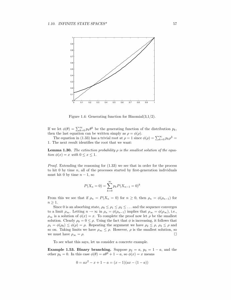
1.10. INFINITE STATE SPACES* 57
0 0.1 0.2 0.3 0.4 0.5 0.6 0.7 0.8 0.9 10
0.1
0.2
0.3
0.4
0.5
0.6
0.7
0.8
0.9
1
Figure 1.4: Generating function for Binomial(3,1/2).
If we let φ(θ) =∑∞
k=0 pkθk be the generating function of the distribution pk,then the last equation can be written simply as ρ = φ(ρ).
The equation in (1.33) has a trivial root at ρ = 1 since φ(ρ) =∑∞
k=0 pkρk =1. The next result identifies the root that we want:
Lemma 1.30. The extinction probability ρ is the smallest solution of the equa-tion φ(x) = x with 0 ≤ x ≤ 1.
Proof. Extending the reasoning for (1.33) we see that in order for the processto hit 0 by time n, all of the processes started by first-generation individualsmust hit 0 by time n− 1, so
P (Xn = 0) =∞∑
k=0
pkP (Xn−1 = 0)k
From this we see that if ρn = P (Xn = 0) for n ≥ 0, then ρn = φ(ρn−1) forn ≥ 1.
Since 0 is an absorbing state, ρ0 ≤ ρ1 ≤ ρ2 ≤ . . . and the sequence convergesto a limit ρ∞. Letting n→∞ in ρn = φ(ρn−1) implies that ρ∞ = φ(ρ∞), i.e.,ρ∞ is a solution of φ(x) = x. To complete the proof now let ρ be the smallestsolution. Clearly ρ0 = 0 ≤ ρ. Using the fact that φ is increasing, it follows thatρ1 = φ(ρ0) ≤ φ(ρ) = ρ. Repeating the argument we have ρ2 ≤ ρ, ρ3 ≤ ρ andso on. Taking limits we have ρ∞ ≤ ρ. However, ρ is the smallest solution, sowe must have ρ∞ = ρ.
To see what this says, let us consider a concrete example.
Example 1.53. Binary branching. Suppose p2 = a, p0 = 1 − a, and theother pk = 0. In this case φ(θ) = aθ2 + 1− a, so φ(x) = x means
0 = ax2 − x + 1− a = (x− 1)(ax− (1− a))

58 CHAPTER 1. MARKOV CHAINS
The roots are 1 and (1− a)/a. If a ≤ 1/2, then the smallest root is 1, while ifa > 1/2 the smallest root is (1− a)/a.
Noting that a ≤ 1/2 corresponds to mean µ ≤ 1 in binary branching moti-vates the following guess:
II. If µ > 1, then there is positive probability of avoiding extinction.
Proof. In view of Lemma 1.30, we only have to show there is a root < 1. Webegin by discarding a trivial case. If p0 = 0, then φ(0) = 0, 0 is the smallestroot, and there is no probability of dying out. If p0 > 0, then φ(0) = p0 > 0.Differentiating the definition of φ, we have
φ′(x) =∞∑
k=1
pk · kxk−1 so φ′(1) =∞∑
k=1
kpk = µ
If µ > 1 then the slope of φ at x = 1 is larger than 1, so if ε is small, thenφ(1− ε) < 1− ε. Combining this with φ(0) > 0 we see there must be a solutionof φ(x) = x between 0 and 1− ε. See the figure in the proof of (7.6).
Turning to the borderline case:
III. If µ = 1 and we exclude the trivial case p1 = 1, then extinction occurs withprobability 1.
Proof. By Lemma 1.30 we only have to show that there is no root < 1. To dothis we note that if p1 < 1, then for y < 1
φ′(y) =∞∑
k=1
pk · kxk−1 <
∞∑k=1
pkk = 1
so if x < 1 then φ(x) = φ(1) −∫ 1
xφ′(y) dy > 1 − (1 − x) = x. Thus φ(x) > x
for all x < 1.
Note that in binary branching with a = 1/2, φ(x) = (1 + x2)/2, so if we tryto solve φ(x) = x we get
0 = 1− 2x + x2 = (1− x)2
i.e., a double root at x = 1. In general when µ = 1, the graph of φ is tangentto the diagonal (x, x) at x = 1. This slows down the convergence of ρn to 1 sothat it no longer occurs exponentially fast.
In more advanced treatments, it is shown that if the offspring distributionhas mean 1 and variance σ2 > 0, then
P1(Xn > 0) ∼ 2nσ2
This is not easy even for the case of binary branching, so we refer to reader toSection 1.9 of Athreya and Ney (1972) for a proof. We mention the result herebecause it allows us to see that the expected time for the process to die out∑
n P1(T0 > n) = ∞. If we modify the branching process, so that p(0, 1) = 1then in the modified process
If µ < 1, 0 is positive recurrent

1.11. CHAPTER SUMMARY 59
If µ = 1, 0 is null recurrentIf µ > 1, 0 is transient
Our final example gives an application of branching processes to queueingtheory.
Example 1.54. M/G/1 queue. We will not be able to explain the nameof this example until we consider Poisson processes in Chapter 2. However,imagine a queue of people waiting to use an automated teller machine. LetXn denote the number of people in line at the moment of the departure of thenth customer. To model this as a Markov chain we let ak be the probabilitythat k customers arrive during one service time and write down the transitionprobability
p(0, k) = ak and p(i, i− 1 + k) = ak for k ≥ 0
with p(i, j) = 0 otherwise.
To explain this, note that if there is a queue, it is reduced by 1 by thedeparture of a customer, but k new customers will come with probability k. Onthe other hand if there is no queue, we must first wait for a customer to comeand the queue that remains at her departure is the number of customers thatarrived during her service time. The pattern becomes clear if we write out afew rows and columns of the matrix:
0 1 2 3 4 5 . . .0 a0 a1 a2 a3 a4 a5
1 a0 a1 a2 a3 a4 a5
2 0 a0 a1 a2 a3 a4
3 0 0 a0 a1 a2 a3
4 0 0 0 a0 a1 a2
If we regard the customers that arrive during a person’s service time to beher children, then this queueing process gives rise to a branching process. Fromthe results above for branching processes we see that if we denote the meannumber of children by µ =
∑k kak, then
If µ < 1, 0 is positive recurrentIf µ = 1, 0 is null recurrentIf µ > 1, 0 is transient
To bring out the parallels between the three examples, note that when µ > 1 orp > 1/2 the process drifts away from 0 and is transient. When µ < 1 or p < 1/2the process drifts toward 0 and is positive recurrent. When µ = 1 or p = 1/2,there is no drift. The process eventually hits 0 but not in finite expected time,so 0 is null recurrent.
1.11 Chapter Summary
A Markov chain with transition probability p is defined by the property thatgiven the present state the rest of the past is irrelevant for predicting the future:
P (Xn+1 = y|Xn = x,Xn−1 = xn−1, . . . , X0 = x0) = p(x, y)

60 CHAPTER 1. MARKOV CHAINS
The m step transition probability
pm(i, j) = P (Xn+m = y|Xn = x)
is the mth power of the matrix p.
Recurrence and transience
The first thing we need to determine about a Markov chain is which statesare recurrent and which are transient. To do this we let Ty = minn ≥ 1 :Xn = y and let
ρxy = Px(Ty <∞)
When x 6= y this is the probability Xn ever visits y starting at x. When x = ythis is the probability Xn returns to y when it starts at y. We restrict to timesn ≥ 1 in the definition of Ty so that we can say: y is recurrent if ρyy = 1 andtransient if ρyy < 1.
Transient states in a finite state space can all be identified using
Theorem 1.5. If ρxy > 0, but ρyx < 1, then x is transient.
Once the transient states are removed we can use
Theorem 1.7. If C is a finite closed and irreducible set, then all states in Care recurrent.
Here A is closed if x ∈ A and y 6∈ A implies p(x, y) = 0, and B is irreducible ifx, y ∈ B implies ρxy > 0.
The keys to the proof of Theorem 1.7 are: (i) If x is recurrent and ρxy > 0then y is recurrent, and (ii) In a finite closed set there has to be at least onerecurrent state. To prove these results, it was useful to know that if N(y) isthe number of visits to y at times n ≥ 1 then
∞∑n=1
pn(x, y) = ExN(y) =ρxy
1− ρyy
so y is recurrent if and only if EyN(y) =∞.
Theorems 1.5 and 1.7 allow us to decompose the state space and simplifythe study of Markov chains.
Theorem 1.8. If the state space S is finite, then S can be written as a disjointunion T∪R1∪· · ·∪Rk, where T is a set of transient states and the Ri, 1 ≤ i ≤ k,are closed irreducible sets of recurrent states.
Stationary distributions
A stationary measure is a nonnegative solution of µp = µ A stationarydistribution is a nonnegative solution of πp = π normalized so that the entriessum to 1. The first question is: do these things exist?
Theorem 1.20. Suppose p is irreducible and recurrent. Let x ∈ S and letTx = infn ≥ 1 : Xn = x.
µx(y) =∞∑
n=0
Px(Xn = y, Tx > n)
defines a stationary measure with 0 < µx(y) <∞ for all y.

1.11. CHAPTER SUMMARY 61
If the state space S is finite and irreducible there is a unique stationary distribu-tion. More generally if ExTx <∞, i.e., x is positive recurrent then µx(y)/ExTx
is a stationary distribution. Since µx(x) = 1 we see that
π(x) =1
ExTx
If there are k states then the stationary distribution π can be computed bythe following procedure. Form a matrix A by taking the first k − 1 columns ofp−I and adding a final column of 1’s. The equations πp = π and π1+· · ·πk = 1are equivalent to
πA =(0 . . . 0 1
)so we have
π =(0 . . . 0 1
)A−1
or π is the bottom row of A−1.In two situations, the stationary distribution is easy to compute. (i) If
the chain is doubly stochastic, i.e.,∑
x p(x, y) = 1, and has k states, then thestationary distribution is uniform π(x) = 1/k. (ii) π is a stationary distributionif the detailed balance condition holds
π(x)p(x, y) = π(y)p(y, x)
Birth and death chains, defined by the condition that p(x, y) = 0 if |x− y| > 1always have stationary distributions with this property. If the state space is`, ` + 1, . . . r then π can be found by setting π(`) = c, solving for π(x) for` < x ≤ r, and then choosing c to make the probabilities sum to 1.
Convergence theorems
Transient states y have pn(x, y) → 0, so to investigate the convergence ofpn(x, y) it is enough, by the decomposition theorem, to suppose the chain isirreducible and all states are recurrent. The period of a state is the greatestcommon divisor of Ix = n ≥ 1 : pn(x, x) > 0. If the period is 1, x is said tobe aperiodic. A simple sufficient condition to be aperiodic is that p(x, x) > 0.To compute the period it is useful to note that if ρxy > 0 and ρyx > 0 then xand y have the same period. In particular all of the states in an irreducible sethave the same period.
The three main results about the asymptotic behavior of Markov chains are:
Theorem 1.19. Suppose p is irreducible, aperiodic, and has a stationary dis-tribution π. Then as n→∞, pn(x, y)→ π(y).
Theorem 1.21. Suppose p is irreducible and recurrent. If Nn(y) be the numberof visits to y up to time n, then
Nn(y)n
→ 1EyTy
Theorem 1.23. Suppose p is irreducible, has stationary distribution π, and∑x |f(x)|π(x) <∞ then
1n
n∑m=1
f(Xm)→∑
x
f(x)π(x)

62 CHAPTER 1. MARKOV CHAINS
Chains with absorbing states
In this case there are two interesting questions. Where does the chain getabsorbed? How long does it take? Let Vy = minn ≥ 0 : Xn = y be the timeof the first visit to y, i.e., now being there at time 0 counts.
Theorem 1.27. Consider a Markov chain with finite state space S. Let a andb be two points in S, and let C = S − a, b. Suppose h(a) = 1, h(b) = 0, andthat for x ∈ C we have
h(x) =∑
y
p(x, y)h(y)
If ρxa + ρxb > 0 for all x ∈ C, then h(x) = Px(Va < Vb).
Let r(x, y) be the part of the matrix p(x, y) with x, y ∈ C. Since h(a) = 1 andh(b) = 0, the equation for h can be written for x ∈ C as
h(x) = r(x, a) +∑
y
r(x, y)h(y)
so if we let v be the column vector with entries r(x, a) then the last equationsays (I − r)h = v and
h = (I − r)−1v.
Theorem 1.28. Consider a Markov chain with finite state space S. Let A ⊂ Sand VA = infn ≥ 0 : Xn ∈ A. Suppose g(a) = 0 for all a ∈ A, and that forx ∈ C = S −A we have
g(x) = 1 +∑
y
p(x, y)g(y)
If Px(VA <∞) > 0 for all x ∈ C, then g(x) = Ex(VA).
Since g(x) = 0 for x ∈ A the equation for g can be written for x ∈ C as
g(x) = 1 +∑
y
r(x, y)g(y)
so if we let ~1 be a column vector consisting of all 1’s then the last equation says(I − r)g = ~1 and
g = (I − r)−1~1.
Since (I − r)−1 = I + r + r2 + . . ., for x, y 6∈ A, (I − r)−1(x, y) is the expectednumber of visits to y starting from x.
1.12 Exercises
Understanding the definitions
1.1. A fair coin is tossed repeatedly with results Y0, Y1, Y2, . . . that are 0 or 1with probability 1/2 each. For n ≥ 1 let Xn = Yn + Yn−1 be the number of 1’sin the (n− 1)th and nth tosses. Is Xn a Markov chain?

1.12. EXERCISES 63
1.2. Five white balls and five black balls are distributed in two urns in such away that each urn contains five balls. At each step we draw one ball from eachurn and exchange them. Let Xn be the number of white balls in the left urn attime n. Compute the transition probability for Xn.
1.3. We repeated roll two four sided dice with numbers 1, 2, 3, and 4 on them.Let Yk be the sum on the kth roll, Sn = Y1 + · · ·+ Yn be the total of the firstn rolls, and Xn = Sn (mod 6). Find the transition probability for Xn.
1.4. The 1990 census showed that 36% of the households in the District ofColumbia were homeowners while the remainder were renters. During the nextdecade 6% of the homeowners became renters and 12% of the renters becamehomeowners. What percentage were homeowners in 2000? in 2010?
1.5. Consider a gambler’s ruin chain with N = 4. That is, if 1 ≤ i ≤ 3,p(i, i + 1) = 0.4, and p(i, i − 1) = 0.6, but the endpoints are absorbing states:p(0, 0) = 1 and p(4, 4) = 1 Compute p3(1, 4) and p3(1, 0).
1.6. A taxicab driver moves between the airport A and two hotels B and Caccording to the following rules. If he is at the airport, he will be at one ofthe two hotels next with equal probability. If at a hotel then he returns to theairport with probability 3/4 and goes to the other hotel with probability 1/4.(a) Find the transition matrix for the chain. (b) Suppose the driver beginsat the airport at time 0. Find the probability for each of his three possiblelocations at time 2 and the probability he is at hotel B at time 3.
1.7. Suppose that the probability it rains today is 0.3 if neither of the last twodays was rainy, but 0.6 if at least one of the last two days was rainy. Let theweather on day n, Wn, be R for rain, or S for sun. Wn is not a Markov chain,but the weather for the last two days Xn = (Wn−1,Wn) is a Markov chainwith four states RR,RS, SR, SS. (a) Compute its transition probability. (b)Compute the two-step transition probability. (c) What is the probability it willrain on Wednesday given that it did not rain on Sunday or Monday.
1.8. Consider the following transition matrices. Identify the transient andrecurrent states, and the irreducible closed sets in the Markov chains. Givereasons for your answers.
(a) 1 2 3 4 51 .4 .3 .3 0 02 0 .5 0 .5 03 .5 0 .5 0 04 0 .5 0 .5 05 0 .3 0 .3 .4
(b) 1 2 3 4 5 61 .1 0 0 .4 .5 02 .1 .2 .2 0 .5 03 0 .1 .3 0 0 .64 .1 0 0 .9 0 05 0 0 0 .4 0 .66 0 0 0 0 .5 .5
(c) 1 2 3 4 51 0 0 0 0 12 0 .2 0 .8 03 .1 .2 .3 .4 04 0 .6 0 .4 05 .3 0 0 0 .7
(d) 1 2 3 4 5 61 .8 0 0 .2 0 02 0 .5 0 0 .5 03 0 0 .3 .4 .3 04 .1 0 0 .9 0 05 0 .2 0 0 .8 06 .7 0 0 .3 0 0

64 CHAPTER 1. MARKOV CHAINS
1.9. Find the stationary distributions for the Markov chains with transitionmatrices:
(a) 1 2 31 .5 .4 .12 .2 .5 .33 .1 .3 .6
(b) 1 2 31 .5 .4 .12 .3 .4 .33 .2 .2 .6
(c) 1 2 31 .6 .4 02 .2 .4 .23 0 .2 .8
1.10. Find the stationary distributions for the Markov chains on 1, 2, 3, 4with transition matrices:
(a)
.7 0 .3 0.6 0 .4 00 .5 0 .50 .4 0 .6
(b)
.7 .3 0 0.2 .5 .3 0.0 .3 .6 .10 0 .2 .8
(c)
.7 0 .3 0.2 .5 .3 0.1 .2 .4 .30 .4 0 .6
(c) The matrix is doubly stochastic so π(i) = 1/4, i = 1, 2, 3, 4.
1.11. Find the stationary distributions for the chains in exercises (a) 1.2, (b)1.3, and (c) 1.7.
1.12. (a) Find the stationary distribution for the transition probability
1 2 3 41 0 2/3 0 1/32 1/3 0 2/3 03 0 1/6 0 5/64 2/5 0 3/5 0
and show that it does not satisfy the detailed balance condition (1.11).(b) Consider
1 2 3 41 0 a 0 1− a2 1− b 0 b 03 0 1− c 0 c4 d 0 1− d 0
and show that there is a stationary distribution satisfying (1.11) if
0 < abcd = (1− a)(1− b)(1− c)(1− d).
1.13. Consider the Markov chain with transition matrix:
1 2 3 41 0 0 0.1 0.92 0 0 0.6 0.43 0.8 0.2 0 04 0.4 0.6 0 0
(a) Compute p2. (b) Find the stationary distributions of p and all of thestationary distributions of p2. (c) Find the limit of p2n(x, x) as n→∞.
1.14. Do the following Markov chains converge to equilibrium?
(a) 1 2 3 41 0 0 1 02 0 0 .5 .53 .3 .7 0 04 1 0 0 0
(b) 1 2 3 41 0 1 .0 02 0 0 0 13 1 0 0 04 1/3 0 2/3 0
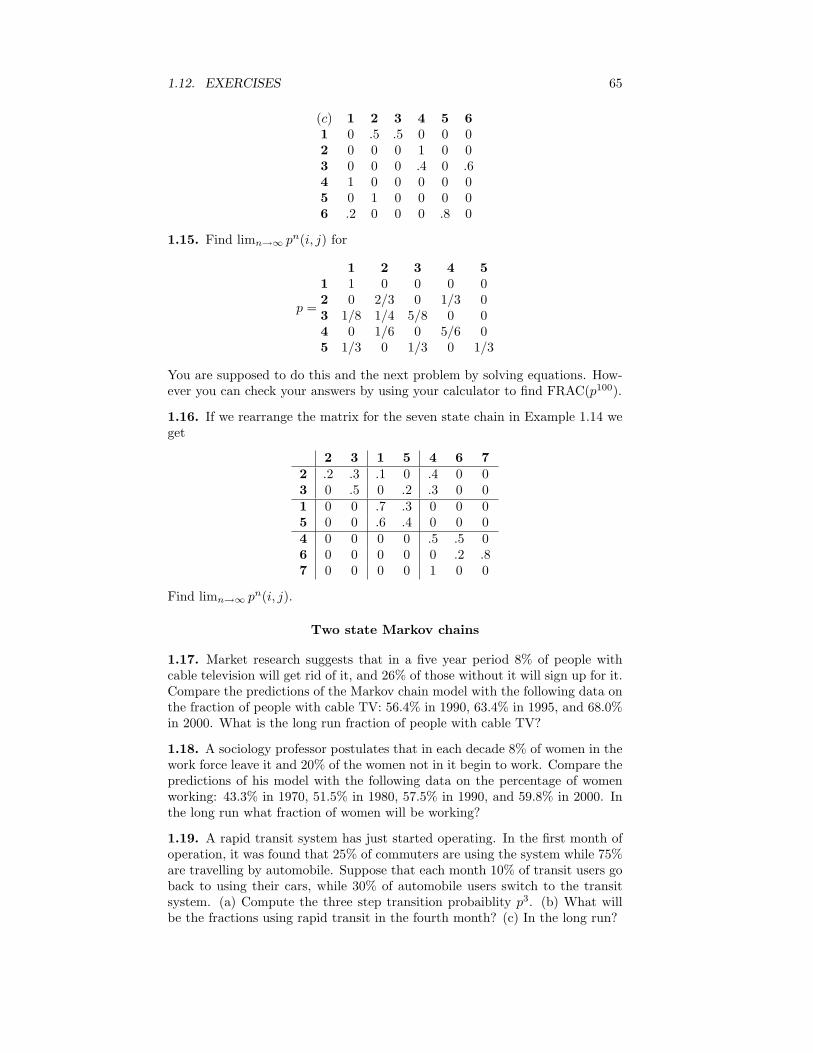
1.12. EXERCISES 65
(c) 1 2 3 4 5 61 0 .5 .5 0 0 02 0 0 0 1 0 03 0 0 0 .4 0 .64 1 0 0 0 0 05 0 1 0 0 0 06 .2 0 0 0 .8 0
1.15. Find limn→∞ pn(i, j) for
p =
1 2 3 4 51 1 0 0 0 02 0 2/3 0 1/3 03 1/8 1/4 5/8 0 04 0 1/6 0 5/6 05 1/3 0 1/3 0 1/3
You are supposed to do this and the next problem by solving equations. How-ever you can check your answers by using your calculator to find FRAC(p100).
1.16. If we rearrange the matrix for the seven state chain in Example 1.14 weget
2 3 1 5 4 6 72 .2 .3 .1 0 .4 0 03 0 .5 0 .2 .3 0 01 0 0 .7 .3 0 0 05 0 0 .6 .4 0 0 04 0 0 0 0 .5 .5 06 0 0 0 0 0 .2 .87 0 0 0 0 1 0 0
Find limn→∞ pn(i, j).
Two state Markov chains
1.17. Market research suggests that in a five year period 8% of people withcable television will get rid of it, and 26% of those without it will sign up for it.Compare the predictions of the Markov chain model with the following data onthe fraction of people with cable TV: 56.4% in 1990, 63.4% in 1995, and 68.0%in 2000. What is the long run fraction of people with cable TV?
1.18. A sociology professor postulates that in each decade 8% of women in thework force leave it and 20% of the women not in it begin to work. Compare thepredictions of his model with the following data on the percentage of womenworking: 43.3% in 1970, 51.5% in 1980, 57.5% in 1990, and 59.8% in 2000. Inthe long run what fraction of women will be working?
1.19. A rapid transit system has just started operating. In the first month ofoperation, it was found that 25% of commuters are using the system while 75%are travelling by automobile. Suppose that each month 10% of transit users goback to using their cars, while 30% of automobile users switch to the transitsystem. (a) Compute the three step transition probaiblity p3. (b) What willbe the fractions using rapid transit in the fourth month? (c) In the long run?

66 CHAPTER 1. MARKOV CHAINS
1.20. A regional health study indicates that from one year to the next, 75%percent of smokers will continue to smoke while 25% will quit. 8% of thosewho stopped smoking will resume smoking while 92% will not. If 70% of thepopulation were smokers in 1995, what fraction will be smokers in 1998? in2005? in the long run?
1.21. Three of every four trucks on the road are followed by a car, while onlyone of every five cars is followed by a truck. What fraction of vehicles on theroad are trucks?
1.22. In a test paper the questions are arranged so that 3/4’s of the time a Trueanswer is followed by a True, while 2/3’s of the time a False answer is followedby a False. You are confronted with a 100 question test paper. Approximatelywhat fraction of the answers will be True.
1.23. In unprofitable times corporations sometimes suspend dividend pay-ments. Suppose that after a dividend has been paid the next one will be paidwith probability 0.9, while after a dividend is suspended the next one will besuspended with probability 0.6. In the long run what is the fraction of dividendsthat will be paid?
1.24. Census results reveal that in the United States 80% of the daughtersof working women work and that 30% of the daughters of nonworking womenwork. (a) Write the transition probability for this model. (b) In the long runwhat fraction of women will be working?
1.25. When a basketball player makes a shot then he tries a harder shot thenext time and hits (H) with probability 0.4, misses (M) with probability 0.6.When he misses he is more conservative the next time and hits (H) with proba-bility 0.7, misses (M) with probability 0.3. (a) Write the transition probabilityfor the two state Markov chain with state space H,M. (b) Find the long-runfraction of time he hits a shot.
1.26. Folk wisdom holds that in Ithaca in the summer it rains 1/3 of the time,but a rainy day is followed by a second one with probability 1/2. Suppose thatIthaca weather is a Markov chain. What is its transition probability?
Chains with three or more states
1.27. (a) Suppose brands A and B have consumer loyalties of .7 and .8, meaningthat a customer who buys A one week will with probability .7 buy it again thenext week, or try the other brand with .3. What is the limiting market share foreach of these products? (b) Suppose now there is a third brand with loyalty .9,and that a consumer who changes brands picks one of the other two at random.What is the new limiting market share for these three products?
1.28. A midwestern university has three types of health plans: a health main-tenance organization (HMO), a preferred provider organization (PPO), and atraditional fee for service plan (FFS). Experience dictates that people changeplans according to the following transition matrix
HMO PPO FFSHMO .85 .1 .05PPO .2 .7 .1FFS .1 .3 .6

1.12. EXERCISES 67
In 2000, the percentages for the three plans were HMO:30%, PPO:25%, andFFS:45%. (a) What will be the percentages for the three plans in 2001? (b)What is the long run fraction choosing each of the three plans?
1.29. Bob eats lunch at the campus food court every week day. He either eatsChinese food, Quesadila, or Salad. His transition matrix is
C Q SC .15 .6 .25Q .4 .1 .5S .1 .3 .6
He had Chinese food on Monday. (a) What are the probabilities for his threemeal choices on Friday (four days later). (b) What are the long run frequenciesfor his three choices?
1.30. The liberal town of Ithaca has a “free bikes for the people program.”You can pick up bikes at the library (L), the coffee shop (C) or the cooperativegrocery store (G). The director of the program has determined that bikes movearound accroding to the following Markov chain
L C GL .5 .2 .3C .4 .5 .1G .25 .25 .5
On Sunday there are an equal number of bikes at each place. (a) What fractionof the bikes are at the three locations on Tuesday? (b) on the next Sunday?(c) In the long run what fraction are at the three locations?
1.31. A plant species has red, pink, or white flowers according to the genotypesRR, RW, and WW, respectively. If each of these genotypes is crossed with apink (RW ) plant then the offspring fractions are
RR RW WWRR .5 .5 0RW .25 .5 .25WW 0 .5 .5
What is the long run fraction of plants of the three types?
1.32. The weather in a certain town is classified as rainy, cloudy, or sunny andchanges according to the following transition probability is
R C SR 1/2 1/4 1/4C 1/4 1/2 1/4S 1/2 1/2 0
In the long run what proportion of days in this town are rainy? cloudy? sunny?
1.33. A sociologist studying living patterns in a certain region determines thatthe pattern of movement between urban (U), suburban (S), and rural areas (R)is given by the following transition matrix.
U S RU .86 .08 .06S .05 .88 .07R .03 .05 .92
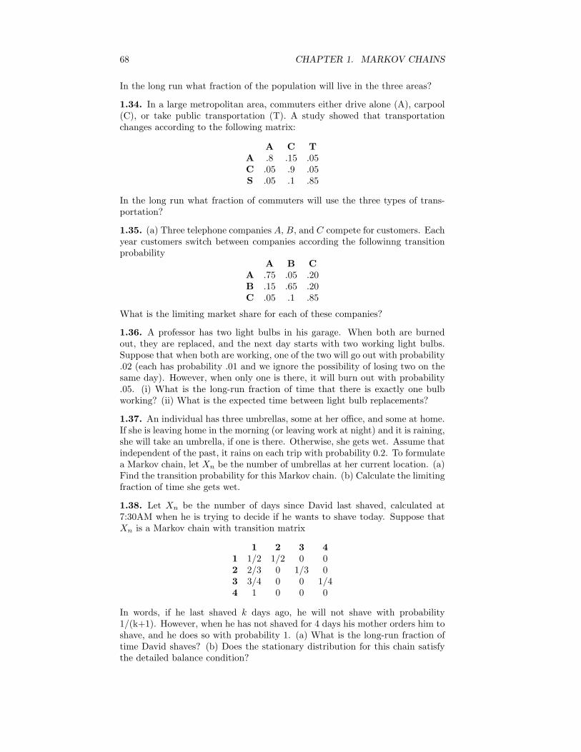
68 CHAPTER 1. MARKOV CHAINS
In the long run what fraction of the population will live in the three areas?
1.34. In a large metropolitan area, commuters either drive alone (A), carpool(C), or take public transportation (T). A study showed that transportationchanges according to the following matrix:
A C TA .8 .15 .05C .05 .9 .05S .05 .1 .85
In the long run what fraction of commuters will use the three types of trans-portation?
1.35. (a) Three telephone companies A, B, and C compete for customers. Eachyear customers switch between companies according the followinng transitionprobability
A B CA .75 .05 .20B .15 .65 .20C .05 .1 .85
What is the limiting market share for each of these companies?
1.36. A professor has two light bulbs in his garage. When both are burnedout, they are replaced, and the next day starts with two working light bulbs.Suppose that when both are working, one of the two will go out with probability.02 (each has probability .01 and we ignore the possibility of losing two on thesame day). However, when only one is there, it will burn out with probability.05. (i) What is the long-run fraction of time that there is exactly one bulbworking? (ii) What is the expected time between light bulb replacements?
1.37. An individual has three umbrellas, some at her office, and some at home.If she is leaving home in the morning (or leaving work at night) and it is raining,she will take an umbrella, if one is there. Otherwise, she gets wet. Assume thatindependent of the past, it rains on each trip with probability 0.2. To formulatea Markov chain, let Xn be the number of umbrellas at her current location. (a)Find the transition probability for this Markov chain. (b) Calculate the limitingfraction of time she gets wet.
1.38. Let Xn be the number of days since David last shaved, calculated at7:30AM when he is trying to decide if he wants to shave today. Suppose thatXn is a Markov chain with transition matrix
1 2 3 41 1/2 1/2 0 02 2/3 0 1/3 03 3/4 0 0 1/44 1 0 0 0
In words, if he last shaved k days ago, he will not shave with probability1/(k+1). However, when he has not shaved for 4 days his mother orders him toshave, and he does so with probability 1. (a) What is the long-run fraction oftime David shaves? (b) Does the stationary distribution for this chain satisfythe detailed balance condition?

1.12. EXERCISES 69
1.39. In a particular county voters declare themselves as members of the Re-publican, Democrat, or Green party. No voters change directly from the Re-publican to Green party or vice versa. Other transitions occur according to thefollowing matrix:
R D GR .85 .15 0D .05 .85 .10G 0 .05 .95
In the long run what fraction of voters will belong to the three parties?
1.40. An auto insurance company classifies its customers in three categories:poor, satisfactory and excellent. No one moves from poor to excellent or fromexcellent to poor in one year.
P S EP .6 .4 0S .1 .6 .3E 0 .2 .8
What is the limiting fraction of drivers in each of these categories?
1.41. Reflecting random walk on the line. Consider the points 1, 2, 3, 4 to bemarked on a straight line. Let Xn be a Markov chain that moves to the rightwith probability 2/3 and to the left with probability 1/3, but subject this timeto the rule that if Xn tries to go to the left from 1 or to the right from 4 itstays put. Find (a) the transition probability for the chain, and (b) the limitingamount of time the chain spends at each site.
1.42. At the end of a month, a large retail store classifies each of its customer’saccounts according to current (0), 30–60 days overdue (1), 60–90 days overdue(2), more than 90 days (3). Their experience indicates that the accounts movefrom state to state according to a Markov chain with transition probabilitymatrix:
0 1 2 30 .9 .1 0 01 .8 0 .2 02 .5 0 0 .53 .1 0 0 .9
In the long run what fraction of the accounts are in each category?
1.43. At the beginning of each day, a piece of equipment is inspected to deter-mine its working condition, which is classified as state 1 = new, 2, 3, or 4 =broken. We assume the state is a Markov chain with the following transitionmatrix:
1 2 3 41 .95 .05 0 02 0 .9 .1 03 0 0 .875 .125
(a) Suppose that a broken machine requires three days to fix. To incorporatethis into the Markov chain we add states 5 and 6 and suppose that p(4, 5) = 1,p(5, 6) = 1, and p(6, 1) = 1. Find the fraction of time that the machine isworking. (b) Suppose now that we have the option of performing preventative
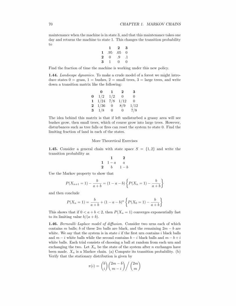
70 CHAPTER 1. MARKOV CHAINS
maintenance when the machine is in state 3, and that this maintenance takes oneday and returns the machine to state 1. This changes the transition probabilityto
1 2 31 .95 .05 02 0 .9 .13 1 0 0
Find the fraction of time the machine is working under this new policy.
1.44. Landscape dynamics. To make a crude model of a forest we might intro-duce states 0 = grass, 1 = bushes, 2 = small trees, 3 = large trees, and writedown a transition matrix like the following:
0 1 2 30 1/2 1/2 0 01 1/24 7/8 1/12 02 1/36 0 8/9 1/123 1/8 0 0 7/8
The idea behind this matrix is that if left undisturbed a grassy area will seebushes grow, then small trees, which of course grow into large trees. However,disturbances such as tree falls or fires can reset the system to state 0. Find thelimiting fraction of land in each of the states.
More Theoretical Exercises
1.45. Consider a general chain with state space S = 1, 2 and write thetransition probability as
1 21 1− a a2 b 1− b
Use the Markov property to show that
P (Xn+1 = 1)− b
a + b= (1− a− b)
P (Xn = 1)− b
a + b
and then conclude
P (Xn = 1) =b
a + b+ (1− a− b)n
P (X0 = 1)− b
a + b
This shows that if 0 < a + b < 2, then P (Xn = 1) converges exponentially fastto its limiting value b/(a + b).
1.46. Bernoulli–Laplace model of diffusion. Consider two urns each of whichcontains m balls; b of these 2m balls are black, and the remaining 2m − b arewhite. We say that the system is in state i if the first urn contains i black ballsand m− i white balls while the second contains b− i black balls and m− b + iwhite balls. Each trial consists of choosing a ball at random from each urn andexchanging the two. Let Xn be the state of the system after n exchanges havebeen made. Xn is a Markov chain. (a) Compute its transition probability. (b)Verify that the stationary distribution is given by
π(i) =(
b
i
)(2m− b
m− i
)/(2m
m
)
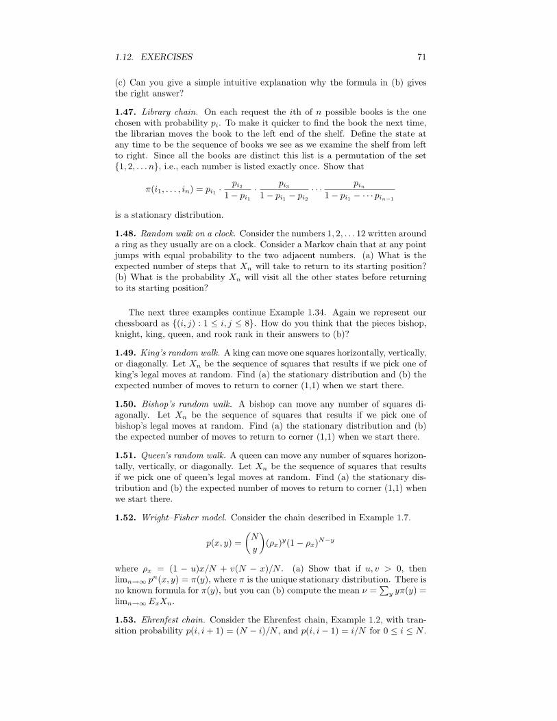
1.12. EXERCISES 71
(c) Can you give a simple intuitive explanation why the formula in (b) givesthe right answer?
1.47. Library chain. On each request the ith of n possible books is the onechosen with probability pi. To make it quicker to find the book the next time,the librarian moves the book to the left end of the shelf. Define the state atany time to be the sequence of books we see as we examine the shelf from leftto right. Since all the books are distinct this list is a permutation of the set1, 2, . . . n, i.e., each number is listed exactly once. Show that
π(i1, . . . , in) = pi1 ·pi2
1− pi1
· pi3
1− pi1 − pi2
· · · pin
1− pi1 − · · · pin−1
is a stationary distribution.
1.48. Random walk on a clock. Consider the numbers 1, 2, . . . 12 written arounda ring as they usually are on a clock. Consider a Markov chain that at any pointjumps with equal probability to the two adjacent numbers. (a) What is theexpected number of steps that Xn will take to return to its starting position?(b) What is the probability Xn will visit all the other states before returningto its starting position?
The next three examples continue Example 1.34. Again we represent ourchessboard as (i, j) : 1 ≤ i, j ≤ 8. How do you think that the pieces bishop,knight, king, queen, and rook rank in their answers to (b)?
1.49. King’s random walk. A king can move one squares horizontally, vertically,or diagonally. Let Xn be the sequence of squares that results if we pick one ofking’s legal moves at random. Find (a) the stationary distribution and (b) theexpected number of moves to return to corner (1,1) when we start there.
1.50. Bishop’s random walk. A bishop can move any number of squares di-agonally. Let Xn be the sequence of squares that results if we pick one ofbishop’s legal moves at random. Find (a) the stationary distribution and (b)the expected number of moves to return to corner (1,1) when we start there.
1.51. Queen’s random walk. A queen can move any number of squares horizon-tally, vertically, or diagonally. Let Xn be the sequence of squares that resultsif we pick one of queen’s legal moves at random. Find (a) the stationary dis-tribution and (b) the expected number of moves to return to corner (1,1) whenwe start there.
1.52. Wright–Fisher model. Consider the chain described in Example 1.7.
p(x, y) =(
N
y
)(ρx)y(1− ρx)N−y
where ρx = (1 − u)x/N + v(N − x)/N . (a) Show that if u, v > 0, thenlimn→∞ pn(x, y) = π(y), where π is the unique stationary distribution. There isno known formula for π(y), but you can (b) compute the mean ν =
∑y yπ(y) =
limn→∞ExXn.
1.53. Ehrenfest chain. Consider the Ehrenfest chain, Example 1.2, with tran-sition probability p(i, i + 1) = (N − i)/N , and p(i, i− 1) = i/N for 0 ≤ i ≤ N .

72 CHAPTER 1. MARKOV CHAINS
Let µn = ExXn. (a) Show that µn+1 = 1 + (1 − 2/N)µn. (b) Use this andinduction to conclude that
µn =N
2+(
1− 2N
)n
(x−N/2)
From this we see that the mean µn converges exponentially rapidly to theequilibrium value of N/2 with the error at time n being (1− 2/N)n(x−N/2).
1.54. Prove that if pij > 0 for all i and j then a necessary and sufficientcondition for the existence of a reversible stationary distribution is
pijpjkpki = pikpkjpji for all i, j, k
Hint: fix i and take πj = cpij/pji.
Exit distributions and times
1.55. The Markov chain associated with a manufacturing process may be de-scribed as follows: A part to be manufactured will begin the process by enteringstep 1. After step 1, 20% of the parts must be reworked, i.e., returned to step1, 10% of the parts are thrown away, and 70% proceed to step 2. After step 2,5% of the parts must be returned to the step 1, 10% to step 2, 5% are scrapped,and 80% emerge to be sold for a profit. (a) Formulate a four-state Markov chainwith states 1, 2, 3, and 4 where 3 = a part that was scrapped and 4 = a partthat was sold for a profit. (b) Compute the probability a part is scrapped inthe production process.
1.56. A bank classifies loans as paid in full (F), in good standing (G), in arrears(A), or as a bad debt (B). Loans move between the categories according to thefollowing transition probability:
F G A BF 1 0 0 0G .1 .8 .1 0A .1 .4 .4 .1B 0 0 0 1
What fraction of loans in good standing are eventually paid in full? What isthe answr for those in arrears?
1.57. A warehouse has a capacity to hold four items. If the warehouse is neitherfull nor empty, the number of items in the warehouse changes whenever a newitem is produced or an item is sold. Suppose that (no matter when we look)the probability that the next event is “a new item is produced” is 2/3 and thatthe new event is a “sale” is 1/3. If there is currently one item in the warehouse,what is the probability that the warehouse will become full before it becomesempty.
1.58. Six children (Dick, Helen, Joni, Mark, Sam, and Tony) play catch. IfDick has the ball he is equally likely to throw it to Helen, Mark, Sam, andTony. If Helen has the ball she is equally likely to throw it to Dick, Joni, Sam,and Tony. If Sam has the ball he is equally likely to throw it to Dick, Helen,Mark, and Tony. If either Joni or Tony gets the ball, they keep throwing it to
1.12. EXERCISES 73
each other. If Mark gets the ball he runs away with it. (a) Find the transitionprobability and classify the states of the chain. (b) Suppose Dick has the ballat the beginning of the game. What is the probability Mark will end up withit?
1.59. Use the second solution in Example 1.48 to compute the expected waitingtimes for the patterns HHH, HHT , HTT , and HTH. Which pattern has thelongest waiting time? Which ones achieve the minimum value of 8?
1.60. Sucker bet. Consider the following gambling game. Player 1 picks a threecoin pattern (for example HTH) and player 2 picks another (say THH). A coinis flipped repeatedly and outcomes are recorded until one of the two patternsappears. Somewhat surprisingly player 2 has a considerable advantage in thisgame. No matter what player 1 picks, player 2 can win with probability ≥ 2/3.Suppose without loss of generality that player 1 picks a pattern that beginswith H:
case Player 1 Player 2 Prob. 2 wins1 HHH THH 7/82 HHT THH 3/43 HTH HHT 2/34 HTT HHT 2/3
Verify the results in the table. You can do this by solving six equations in sixunknowns but this is not the easiest way.
1.61. At the New York State Fair in Syracuse, Larry encounters a carnivalgame where for one dollar he may buy a single coupon allowing him to play aguessing game. On each play, Larry has an even chance of winning or losing acoupon. When he runs out of coupons he loses the game. However, if he cancollect three coupons, he wins a surprise. (a) What is the probability Larry willwin the surprise? (b) What is the expected number of plays he needs to win orlose the game.
1.62. The Megasoft company gives each of its employees the title of program-mer (P) or project manager (M). In any given year 70% of programmers remainin that position 20% are promoted to project manager and 10% are fired (stateX). 95% of project managers remain in that position while 5% are fired. Howlong on the average does a programmer work before they are fired?
1.63. At a nationwide travel agency, newly hired employees are classified asbeginners (B). Every six months the performance of each agent is reviewed.Past records indicate that transitions through the ranks to intermediate (I) andqualified (Q) are according to the following Markov chain, where F indicatesworkers that were fired:
B I Q FB .45 .4 0 .15I 0 .6 .3 .1Q 0 0 1 0F 0 0 0 1
(a) What fraction are eventually promoted? (b) What is the expected timeuntil a beginner is fired or becomes qualified?

74 CHAPTER 1. MARKOV CHAINS
1.64. At a manufacturing plant, employees are classified as trainee (R), tech-nician (T) or supervisor (S). Writing Q for an employee who quits we modeltheir progress through the ranks as a Markov chain with transition probability
R T S QR .2 .6 0 .2T 0 .55 .15 .3S 0 0 1 0Q 0 0 0 1
(a) What fraction of recruits eventually make supervisor? (b) What is theexpected time until a trainee auits or becomes supervisor?
1.65. Customers shift between variable rate loans (V), thirty year fixed-rateloans (30), fifteen year fixed-rate loans (15), or enter the states paid in full (P),or foreclosed according to the following transition matrix:
V 30 15 P fV .55 .35 0 .05 .0530 .15 .54 .25 .05 .0115 .20 0 .75 .04 .01P 0 0 0 1 0F 0 0 0 0 1
(a) For each of the three loan types find (a) the expected time until paid orforeclosed. (b) the probability the loan is paid.
1.66. Brother–sister mating. In this genetics scheme two individuals (one maleand one female) are retained from each generation and are mated to give thenext. If the individuals involved are diploid and we are interested in a trait withtwo alleles, A and a, then each individual has three possible states AA, Aa, aaor more succinctly 2, 1, 0. If we keep track of the sexes of the two individuals thechain has nine states, but if we ignore the sex there are just six: 22, 21, 20, 11,10, and 00. (a) Assuming that reproduction corresponds to picking one letterat random from each parent, compute the transition probability. (b) 22 and 00are absorbing states for the chain. Show that the probability of absorption in22 is equal to the fraction of A’s in the state. (c) Let T = minn ≥ 0 : Xn =22 or 00 be the absorption time. Find ExT for all states x.
1.67. Roll a fair die repeatedly and let Y1, Y2, . . . be the resulting numbers.Let Xn = |Y1, Y2, . . . , Yn| be the number of values we have seen in the first nrolls for n ≥ 1 and set X0 = 0. Xn is a Markov chain. (a) Find its transitionprobability. (b) Let T = minn : Xn = 6 be the number of trials we need tosee all 6 numbers at least once. Find ET .
1.68. Coupon collector’s problem. We are interested now in the time it takesto collect a set of N baseball cards. Let Tk be the number of cards we have tobuy before we have k that are distinct. Clearly, T1 = 1. A little more thoughtreveals that if each time we get a card chosen at random from all N possibilities,then for k ≥ 1, Tk+1− Tk has a geometric distribution with success probability(N − k)/N . Use this to show that the mean time to collect a set of N baseballcards is ≈ N log N , while the variance is ≈ N2
∑∞k=1 1/k2.

1.12. EXERCISES 75
1.69. Algorthmic efficiency. The simplex method minimizes linear functions bymoving between extreme points of a polyhedral region so that each transitiondecreases the objective function. Suppose there are n extreme points and theyare numbered in increasing order of their values. Consider the Markov chain inwhich p(1, 1) = 1 and p(i, j) = 1/i− 1 for j < i. In words, when we leave j weare equally likely to go to any of the extreme points with better value. (a) Use(1.25) to show that for i > 1
EiT1 = 1 + 1/2 + · · ·+ 1/(i− 1)
(b) Let Ij = 1 if the chain visits j on the way from n to 1. Show that for j < n
P (Ij = 1|Ij+1, . . . In) = 1/j
to get another proof of the result and conclude that I1, . . . In−1 are independent.
Infinite State Space
1.70. General birth and death chains. The state space is 0, 1, 2, . . . and thetransition probability has
p(x, x + 1) = px
p(x, x− 1) = qx for x > 0p(x, x) = rx for x ≥ 0
while the other p(x, y) = 0. Let Vy = minn ≥ 0 : Xn = y be the time of thefirst visit to y and let hN (x) = Px(VN < V0). By considering what happens onthe first step, we can write
hN (x) = pxhN (x + 1) + rxhN (x) + qxhN (x− 1)
Set hN (1) = cN and solve this equation to conclude that 0 is recurrent if andonly if
∑∞y=1
∏y−1x=1 qx/px =∞ where by convention
∏0x=1 = 1.
1.71. To see what the conditions in the last problem say we will now considersome concrete examples. Let px = 1/2, qx = e−cx−α
/2, rx = 1/2 − qx forx ≥ 1 and p0 = 1. For large x, qx ≈ (1 − cx−α)/2, but the exponentialformulation keeps the probabilities nonnegative and makes the problem easierto solve. Show that the chain is recurrent if α > 1 or if α = 1 and c ≤ 1 but istransient otherwise.
1.72. Consider the Markov chain with state space 0, 1, 2, . . . and transitionprobability
p(m,m + 1) =12
(1− 1
m + 2
)for m ≥ 0
p(m,m− 1) =12
(1 +
1m + 2
)for m ≥ 1
and p(0, 0) = 1− p(0, 1) = 3/4. Find the stationary distribution π.
1.73. Consider the Markov chain with state space 1, 2, . . . and transitionprobability
p(m,m + 1) = m/(2m + 2) for m ≥ 1p(m,m− 1) = 1/2 for m ≥ 2
p(m,m) = 1/(2m + 2) for m ≥ 2
and p(1, 1) = 1− p(1, 2) = 3/4. Show that there is no stationary distribution.

76 CHAPTER 1. MARKOV CHAINS
1.74. Consider the aging chain on 0, 1, 2, . . . in which for any n ≥ 0 theindividual gets one day older from n to n + 1 with probability pn but dies andreturns to age 0 with probability 1 − pn. Find conditions that guarantee that(a) 0 is recurrent, (b) positive recurrent. (c) Find the stationary distribution.
1.75. The opposite of the aging chain is the renewal chain with state space0, 1, 2, . . . in which p(i, i− 1) = 1 when i > 0. The only nontrivial part of thetransition probability is p(0, i) = pi. Show that this chain is always recurrentbut is positive recurrent if and only if
∑n npn <∞.
1.76. Consider a branching process as defined in Example 7.2, in which eachfamily has exactly three children, but invert Galton and Watson’s original mo-tivation and ignore male children. In this model a mother will have an averageof 1.5 daughters. Compute the probability that a given woman’s descendentswill die out.
1.77. Consider a branching process as defined in Example 7.2, in which eachfamily has a number of children that follows a shifted geometric distribution:pk = p(1 − p)k for k ≥ 0, which counts the number of failures before the firstsuccess when success has probability p. Compute the probability that startingfrom one individual the chain will be absorbed at 0.

Chapter 2
Poisson Processes
2.1 Exponential Distribution
To prepare for our discussion of the Poisson process, we need to recall thedefinition and some of the basic properties of the exponential distribution. Arandom variable T is said to have an exponential distribution with rateλ, or T = exponential(λ), if
P (T ≤ t) = 1− e−λt for all t ≥ 0 (2.1)
Here we have described the distribution by giving the distribution functionF (t) = P (T ≤ t). We can also write the definition in terms of the densityfunction fT (t) which is the derivative of the distribution function.
fT (t) =
λe−λt for t ≥ 00 for t < 0
(2.2)
Integrating by parts with f(t) = t and g′(t) = λe−λt,
ET =∫
t fT (t) dt =∫ ∞
0
t · λe−λt dt
= −te−λt∣∣∞0
+∫ ∞
0
e−λt dt = 1/λ (2.3)
Integrating by parts with f(t) = t2 and g′(t) = λe−λt, we see that
ET 2 =∫
t2 fT (t) dt =∫ ∞
0
t2 · λe−λt dt
= −t2e−λt∣∣∞0
+∫ ∞
0
2te−λt dt = 2/λ2 (2.4)
by the formula for ET . So the variance
var (T ) = ET 2 − (ET )2 = 1/λ2 (2.5)
While calculus is required to know the exact values of the mean and variance,it is easy to see how they depend on λ. Let T = exponential(λ), i.e., have an
77

78 CHAPTER 2. POISSON PROCESSES
exponential distribution with rate λ, and let S = exponential(1). To see thatS/λ has the same distribution as T , we use (2.1) to conclude
P (S/λ ≤ t) = P (S ≤ λt) = 1− e−λt = P (T ≤ t)
Recalling that if c is any number then E(cX) = cEX and var (cX) = c2 var (X),we see that
ET = ES/λ var (T ) = var (S)/λ2
Lack of memory property. It is traditional to formulate this property interms of waiting for an unreliable bus driver. In words, “if we’ve been waitingfor t units of time then the probability we must wait s more units of time is thesame as if we haven’t waited at all.” In symbols
P (T > t + s|T > t) = P (T > s) (2.6)
To prove this we recall that if B ⊂ A, then P (B|A) = P (B)/P (A), so
P (T > t + s|T > t) =P (T > t + s)
P (T > t)=
e−λ(t+s)
e−λt= e−λs = P (T > s)
where in the third step we have used the fact ea+b = eaeb.
Exponential races. Let S = exponential(λ) and T = exponential(µ) beindependent. In order for the minimum of S and T to be larger than t, each ofS and T must be larger than t. Using this and independence we have
P (min(S, T ) > t) = P (S > t, T > t) = P (S > t)P (T > t)
= e−λte−µt = e−(λ+µ)t (2.7)
That is, min(S, T ) has an exponential distribution with rate λ + µ. Thelast calculation extends easily to a sequence of independent random variablesT1, . . . , Tn where Ti = exponential(λi).
P (min(T1, . . . , Tn) > t) = P (T1 > t, . . . Tn > t)
=n∏
i=1
P (Ti > t) =n∏
i=1
e−λit = e−(λ1+···+λn)t (2.8)
That is, the minimum, min(T1, . . . , Tn), of several independent exponentials hasan exponential distribution with rate equal to the sum of the rates λ1 + · · ·λn.
In the last paragraph we have computed the duration of a race between ex-ponentially distributed random variables. We will now consider: “Who finishesfirst?” Going back to the case of two random variables, we break things downaccording to the value of S and then using independence with our formulas(2.1) and (2.2) for the distribution and density functions, to conclude
P (S < T ) =∫ ∞
0
fS(s)P (T > s) ds
=∫ ∞
0
λe−λse−µs ds
=λ
λ + µ
∫ ∞
0
(λ + µ)e−(λ+µ)s ds =λ
λ + µ(2.9)

2.1. EXPONENTIAL DISTRIBUTION 79
where on the last line we have used the fact that (λ + µ)e−(λ+µ)s is a densityfunction and hence must integrate to 1.
From the calculation for two random variables, you should be able to guessthat if T1, . . . , Tn are independent exponentials, then
P (Ti = min(T1, . . . , Tn)) =λi
λ1 + · · ·+ λn(2.10)
That is, the probability of i finishing first is proportional to its rate.
Proof. Let S = Ti and U be the minimum of Tj , j 6= i. (2.8) implies that U isexponential with parameter
µ = (λ1 + · · ·+ λn)− λi
so using the result for two random variables
P (Ti = min(T1, . . . , Tn)) = P (S < U) =λi
λi + µ=
λi
λ1 + · · ·+ λn
proves the desired result.
Let I be the (random) index of the Ti that is smallest. In symbols,
P (I = i) =λi
λ1 + · · ·+ λn
You might think that the Ti’s with larger rates might be more likely to winearly. However,
I and V = minT1, . . . Tn are independent. (2.11)
Proof. Let fi,V (t) be the density function for V on the set I = i. In order for ito be first at time t, Ti = t and the other Tj > t so
fi,V (t) = λie−λit ·
∏j 6=i
e−λjt
=λi
λ1 + · · ·+ λn· (λ1 + · · ·+ λn)e−(λ1+·+λn)t
= P (I = i) · fV (t)
since V has an exponential(λ1 + · · ·+ λn) distribution.
Our final fact in this section concerns sums of exponentials.
Theorem 2.1. Let τ1, τ2, . . . be independent exponential(λ). The sum Tn =τ1 + · · · + τn has a gamma(n, λ) distribution. That is, the density function ofTn is given by
fTn(t) = λe−λt · (λt)n−1
(n− 1)!for t ≥ 0 (2.12)
and 0 otherwise.

80 CHAPTER 2. POISSON PROCESSES
Proof. The proof is by induction on n. When n = 1, T1 has an exponential(λ)distribution. Recalling that the 0th power of any positive number is 1, and byconvention we set 0!=1, the formula reduces to
fT1(t) = λe−λt
and we have shown that our formula is correct for n = 1.To do the induction step, suppose that the formula is true for n. The sum
Tn+1 = Tn + τn+1, so breaking things down according to the value of Tn, andusing the independence of Tn and tn+1, we have
fTn+1(t) =∫ t
0
fTn(s)ftn+1(t− s) ds
Plugging the formula from (2.12) in for the first term and the exponentialdensity in for the second and using the fact that eaeb = ea+b with a = −λs andb = −λ(t− s) gives∫ t
0
λe−λs (λs)n−1
(n− 1)!· λe−λ(t−s) ds = e−λtλn
∫ t
0
sn−1
(n− 1)!ds
= λe−λt λntn
n!
which completes the proof.
2.2 Defining the Poisson Process
In this section we will give two definitions of the Poisson process with rateλ. The first, which will be our official definition, is nice because it allows us toconstruct the process easily.
Definition. Let τ1, τ2, . . . be independent exponential(λ) random variables.Let Tn = τ1 + · · ·+ τn for n ≥ 1, T0 = 0, and define N(s) = maxn : Tn ≤ s.
We think of the τn as times between arrivals of customers at a bank, so Tn =τ1 + · · · + τn is the arrival time of the nth customer, and N(s) is the numberof arrivals by time s. To check the last interpretation, consider the followingexample:
× × × × ×0 T1 T2 T3 T4 s T5
τ1 τ2 τ3 τ4τ5
Figure 2.1: Poisson process definitions.
and note that N(s) = 4 when T4 ≤ s < T5, that is, the 4th customer has arrivedby time s but the 5th has not.
Recall that X has a Poisson distribution with mean λ, or X = Poisson(λ),for short, if
P (X = n) = e−λ λn
n!for n = 0, 1, 2, . . .

2.2. DEFINING THE POISSON PROCESS 81
To explain why N(s) is called the Poisson process rather than the exponentialprocess, we will compute the distribution of N(s).
Lemma 2.2. N(s) has a Poisson distribution with mean λs.
Proof. Now N(s) = n if and only if Tn ≤ s < Tn+1; i.e., the nth customerarrives before time s but the (n+1)th after s. Breaking things down accordingto the value of Tn = t and noting that for Tn+1 > s, we must have τn+1 > s− t,and τn+1 is independent of Tn, it follows that
P (N(s) = n) =∫ s
0
fTn(t)P (tn+1 > s− t) dt
Plugging in (2.12) now, the last expression is
=∫ s
0
λe−λt (λt)n−1
(n− 1)!· e−λ(s−t) dt
=λn
(n− 1)!e−λs
∫ s
0
tn−1 dt = e−λs (λs)n
n!
which proves the desired result.
Since this is our first mention of the Poisson distribution, we pause to derivesome of its properties.
Theorem 2.3. For any k ≥ 1
EX(X − 1) · · · (X − k + 1) = λk (2.13)
and hence var (X) = λ
Proof. X(X − 1) · · · (X − k + 1) = 0 if X ≤ k − 1 so
EX(X − 1) · · · (X − k + 1) =∞∑
j=k
e−λ λj
j!j(j − 1) · · · (j − k + 1)
= λk∞∑
j=k
e−λ λj−k
(j − k)!= λk
since the sum gives the total mass of the Poisson distribution. Using var (X) =E(X(X − 1)) + EX − (EX)2 we conclude
var (X) = λ2 + λ− (λ)2 = λ
Theorem 2.4. If Xi are independent Poissson(λi) then
X1 + · · ·+ Xk = Poisson(λ1 + · · ·+ λn).
Proof. It suffices to prove the result for k = 2, for then the general result followsby induction.
P (X1 + X2 = n) =n∑
m=0
P (X1 = m)P (X2 = n−m)
=n∑
m=0
e−λ1(λ1)m
m!· e−λ2
(λ2)n−m
(n−m)!

82 CHAPTER 2. POISSON PROCESSES
Knowing the answer we want, we can rewrite the last expression as
e−(λ1+λ2)(λ1 + λ2)n
n!·
n∑m=0
(n
m
)(λ1
λ1 + λ2
)m(λ2
λ1 + λ2
)n−m
The sum is 1, since it is the sum of all the probabilities for a binomial(n, p)distribution with p = λ1/(λ1 + λ2). The term outside the sum is the desiredPoisson probability, so have proved the desired result.
The property of the Poisson process in Lemma 2.2 is the first part of oursecond definition. To start to develop the second part we prove a Markovproperty:
Lemma 2.5. N(t+s)−N(s), t ≥ 0 is a rate λ Poisson process and independentof N(r), 0 ≤ r ≤ s.
Why is this true? Suppose for concreteness (and so that we can use Figure2.2 at the beginning of this section again) that by time s there have been fourarrivals T1, T2, T3, T4 that occurred at times t1, t2, t3, t4. We know that thewaiting time for the fifth arrival must have τ5 > s − t4, but by the lack ofmemory property of the exponential distribution (2.6)
P (τ5 > s− t4 + t|τ5 > s− t4) = P (τ5 > t) = e−λt
This shows that the distribution of the first arrival after s is exponential(λ)and independent of T1, T2, T3, T4. It is clear that τ6, τ7, . . . are independentof T1, T2, T3, T4, and τ5. This shows that the interarrival times after s areindependent exponential(λ), and hence that N(t+ s)−N(s), t ≥ 0 is a Poissonprocess.
From Lemma 2.5 we get easily the following:
Lemma 2.6. N(t) has independent increments: if t0 < t1 < . . . < tn, then
N(t1)−N(t0), N(t2)−N(t1), . . . N(tn)−N(tn−1) are independent
Why is this true? Lemma 2.5 implies that N(tn)−N(tn−1) is independent ofN(r), r ≤ tn−1 and hence of N(tn−1)−N(tn−2), . . . N(t1)−N(t0). The desiredresult now follows by induction.
We are now ready for our second definition. It is in terms of the processN(s) : s ≥ 0 that counts the number of arrivals in [0, s].
Theorem 2.7. If N(s), s ≥ 0 is a Poisson process, then(i) N(0) = 0,(ii) N(t + s)−N(s) = Poisson(λt), and(iii) N(t) has independent increments.
Conversely, if (i), (ii), and (iii) hold, then N(s), s ≥ 0 is a Poisson process.
Why is this true? Clearly, (i) holds. Lemmas 2.2 and 2.6 prove (ii) and (iii).To start to prove the converse, let Tn be the time of the nth arrival. The firstarrival occurs after time t if and only if there were no arrivals in [0, t]. So usingthe formula for the Poisson distribution
P (τ1 > t) = P (N(t) = 0) = e−λt

2.2. DEFINING THE POISSON PROCESS 83
This shows that τ1 = T1 is exponential(λ). For τ2 = T2 − T1 we note that
P (τ2 > t|τ1 = s) = P ( no arrival in (s, s + t] |τ1 = s)= P (N(t + s)−N(s) = 0|N(r) = 0 for r < s,N(s) = 1)
= P (N(t + s)−N(s) = 0) = e−λt
by the independent increments property in (iii), so τ2 is exponential(λ) and in-dependent of τ1. Repeating this argument we see that τ1, τ2, . . . are independentexponential(λ).
Up to this point we have been concerned with the mechanics of defining thePoisson process, so the reader may be wondering:
Why is the Poisson process important for applications?
Our answer is based on the Poisson approximation to the binomial. Supposethat each of the n students on Duke campus flips coins with probability λ/n ofheads to decide if they will go to the Great Hall (food court) between 12:17 and12:18 . The probability that exactly k students will go during the one-minutetime interval is given by the binomial(n, λ/n) distribution
n(n− 1) · · · (n− k + 1)k!
(λ
n
)k (1− λ
n
)n−k
(2.14)
Theorem 2.8. If n is large the binomial(n, λ/n) distribution is approximatelyPoisson(λ).
Proof. Exchanging the numerators of the first two fractions and breaking thelast term into two, (2.14) becomes
λk
k!· n(n− 1) · · · (n− k + 1)
nk·(
1− λ
n
)n(1− λ
n
)−k
(2.15)
Considering the four terms separately, we have
(i) λk/k! does not depend on n.
(ii) There are k terms on the top and k terms on the bottom, so we can writethis fraction as
n
n· n− 1
n· · · n− k + 1
n
For any j we have (n− j)/n→ 1 as n→∞, so the second term converges to 1as n→∞.
(iii) Skipping to the last term in (2.15), λ/n→ 0, so 1− λ/n→ 1. The power−k is fixed so (
1− λ
n
)−k
→ 1−k = 1
(iv) We broke off the last piece to make it easier to invoke one of the famousfacts of calculus:
(1− λ/n)n → e−λ as n→∞.
If you haven’t seen this before, recall that
log(1− x) = −x + x2/2 + . . .

84 CHAPTER 2. POISSON PROCESSES
so we have n log(1− λ/n) = −λ + λ2/n + . . .→ λ as n→∞.Combining (i)–(iv), we see that (2.15) converges to
λk
k!· 1 · e−λ · 1
which is the Poisson distribution with mean λ.
By extending the last argument we can also see why the number of individ-uals that arrive in two disjoint time intervals should be independent. Using themultinomial instead of the binomial, we see that the probability j people willgo between 12:17 and 12:18 and k people will go between 12:31 and 12:33 is
n!j!k!(n− j − k)!
(λ
n
)j (2λ
n
)k (1− 3λ
n
)n−(j+k)
Rearranging gives
(λ)j
j!· (2λ)k
k!· n(n− 1) · · · (n− j − k + 1)
nj+k·(
1− 3λ
n
)n−(j+k)
Reasoning as before shows that when n is large, this is approximately
(λ)j
j!· (2λ)k
k!· 1 · e−3λ
Writing e−λ = e−λ/3e−2λ/3 and rearranging we can write the last expression as
e−λ λj
j!· e−2λ (2λ)k
k!
This shows that the number of arrivals in the two time intervals we chose areindependent Poissons with means λ and 2λ.
The last proof can be easily generalized to show that if we divide the hourbetween 12:00 and 1:00 into any number of intervals, then the arrivals areindependent Poissons with the right means. However, the argument gets verymessy to write down.
More realistic models.
Two of the weaknesses of the derivation above are:
(i) All students are assumed to have exactly the same probability of going tothe Great Hall.
(ii) The probability of going in a given time interval is a constant multiple ofthe length of the interval, so the arrival rate of customers is constant duringthe hour. In reality there is a large influx of people between 11:30 and 11:45soon after the end of 10:10-11:25 classes.
(i) is a very strong assumption but can be weakened by using a more generalPoisson approximation result like the following:
Theorem 2.9. Let Xn,m, 1 ≤ m ≤ n be independent random variables withP (Xm = 1) = pm and P (Xm = 0) = 1− pm. Let
Sn = X1 + · · ·+ Xn, λn = ESn = p1 + · · ·+ pn,

2.2. DEFINING THE POISSON PROCESS 85
and Zn = Poisson(λn). Then for any set A
|P (Sn ∈ A)− P (Zn ∈ A)| ≤n∑
m=1
p2m
Why is this true? If X and Y are integer valued random variables then forany set A
|P (X ∈ A)− P (Y ∈ A)| ≤ 12
∑n
|P (X = n)− P (Y = n)|
The right-hand side is called the total variation distance between the twodistributions and is denoted ‖X − Y ‖. If P (X = 1) = p, P (X = 0) = 1 − p,and Y = Poisson(p) then∑
n
|P (X = n)− P (Y = n)| = |(1− p)− e−p|+ |p− pe−p|+ 1− (1 + p)e−p
Since 1 ≥ e−p ≥ 1− p the right-hand side is
e−p − 1 + p + p− pe−p + 1− e−p − pe−p = 2p(1− e−p ≤ 2p2
Let Ym = Poisson(pm) be independent. At this point we have shown ‖Xi −Yi‖ ≤ p2
i . With a little work one can show
‖(X1 + · · ·+ Xn)− (Y1 + · · ·+ Yn)‖
‖(X1, · · · , Xn)− (Y1, · · · , Yn)‖ ≤n∑
m=1
‖Xm − Ym‖
and the desired result follows.
Theorem 2.9 is useful because it gives a bound on the difference betweenthe distribution of Sn and the Poisson distribution with mean λn = ESn. Tobound the bound it is useful to note that
n∑m=1
p2m ≤ max
kpk
(n∑
m=1
pm
)so the approximation is good if maxk pk is small. This is similar to the usualheuristic for the normal distribution: the sum is due to small contributions froma large number of variables. However, here small means that it is nonzero withsmall probability. When a contribution is made it is equal to 1.
The last results handles problem (i). To address the problem of varyingarrival rates mentioned in (ii), we generalize the definition.
Nonhomogeneous Poisson processes. We say that N(s), s ≥ 0 is aPoisson process with rate λ(r) if
(i) N(0) = 0,(ii) N(t) has independent increments, and(iii) N(t)−N(s) is Poisson with mean
∫ t
sλ(r) dr.
The first definition does not work well in this setting since the interarrivaltimes τ1, τ2, . . . are no longer exponentially distributed or independent. Todemonstrate the first claim, we note that
P (τ1 > t) = P (N(t) = 0) = e−R t0 λ(s) ds

86 CHAPTER 2. POISSON PROCESSES
since N(t) is Poisson with mean µ(t) =∫ t
0λ(s) ds. Differentiating gives the
density function
P (τ1 = t) = − d
dtP (t1 > t) = λ(t)e−
R t0 λ(s) ds = λ(t)e−µ(t)
Generalizing the last computation shows that the joint distribution
fT1,T2(u, v) = λ(u)e−µ(u) · λ(v)e−(µ(v)−µ(u))
Changing variables, s = u, t = v − u, the joint density
fτ1,τ2(s, t) = λ(s)e−µ(s) · λ(s + t)e−(µ(s+t)−µ(s))
so τ1 and τ2 are not independent when λ(s) is not constant.
2.3 Compound Poisson Processes
In this section we will embellish our Poisson process by associating an indepen-dent and identically distributed (i.i.d.) random variable Yi with each arrival.By independent we mean that the Yi are independent of each other and of thePoisson process of arrivals. To explain why we have chosen these assumptions,we begin with two examples for motivation.
Example 2.1. Consider the McDonald’s restaurant on Route 13 in the south-ern part of Ithaca. By arguments in the last section, it is not unreasonable toassume that between 12:00 and 1:00 cars arrive according to a Poisson processwith rate λ. Let Yi be the number of people in the ith vehicle. There might besome correlation between the number of people in the car and the arrival time,e.g., more families come to eat there at night, but for a first approximation itseems reasonable to assume that the Yi are i.i.d. and independent of the Poissonprocess of arrival times.
Example 2.2. Messages arrive at a central computer to be transmitted acrossthe Internet. If we imagine a large number of users working at terminals con-nected to a central computer, then the arrival times of messages can be modeledby a Poisson process. If we let Yi be the size of the ith message, then againit is reasonable to assume Y1, Y2, . . . are i.i.d. and independent of the Poissonprocess of arrival times.
Having introduced the Yi’s, it is natural to consider the sum of the Yi’s wehave seen up to time t:
S(t) = Y1 + · · ·+ YN(t)
where we set S(t) = 0 if N(t) = 0. In Example 2.1, S(t) gives the number ofcustomers that have arrived up to time t. In Example 2.2, S(t) represents thetotal number of bytes in all of the messages up to time t. In each case it isinteresting to know the mean and variance of S(t).
Theorem 2.10. Let Y1, Y2, . . . be independent and identically distributed, letN be an independent nonnegative integer valued random variable, and let S =Y1 + · · ·+ YN with S = 0 when N = 0.
(i) If E|Yi|, EN <∞, then ES = EN · EYi.
(ii) If EY 2i , EN2 <∞, then var (S) = EN var (Yi) + var (N)(EYi)2.
(iii) If N is Poisson(λ), then var (S) = λEY 2i .
2.3. COMPOUND POISSON PROCESSES 87
Why is this reasonable? The first of these is natural since if N = n isnonrandom ES = nEYi. (i) then results by setting n = EN . The formula in(ii) is more complicated but it clearly has two of the necessary properties:
If N = n is nonrandom, var (S) = n var (Yi).
If Yi = c is nonrandom var (S) = c2 var (N).
Combining these two observations, we see that EN var (Yi) is the contribu-tion to the variance from the variability of the Yi, while var (N)(EYi)2 is thecontribution from the variability of N .
Proof. When N = n, S = X1 + · · · + Xn has ES = nEYi. Breaking thingsdown according to the value of N ,
ES =∞∑
n=0
E(S|N = n) · P (N = n)
=∞∑
n=0
nEYi · P (N = n) = EN · EYi
For the second formula we note that when N = n, S = X1 + · · · + Xn hasvar (S) = n var (Yi) and hence,
E(S2|N = n) = n var (Yi) + (nEYi)2
Computing as before we get
ES2 =∞∑
n=0
E(S2|N = n) · P (N = n)
=∞∑
n=0
n · var (Yi) + n2(EYi)2 · P (N = n)
= (EN) · var (Yi) + EN2 · (EYi)2
To compute the variance now, we observe that
var (S) = ES2 − (ES)2
= (EN) · var (Yi) + EN2 · (EYi)2 − (EN · EYi)2
= (EN) · var (Yi) + var (N) · (EYi)2
where in the last step we have used var (N) = EN2 − (EN)2 to combine thesecond and third terms.
For part (iii), we note that in the special case of the Poisson, we have EN =λ and var (N) = λ, so the result follows from var (Yi) + (EYi)2 = EY 2
i .
For a concrete example of the use of Theorem 2.10 consider
Example 2.3. Suppose that the number of customers at a liquor store in aday has a Poisson distribution with mean 81 and that each customer spends anaverage of $8 with a standard deviation of $6. It follows from (i) in Theorem2.10 that the mean revenue for the day is 81 · $8 = $648. Using (iii), we seethat the variance of the total revenue is
81 ·($6)2 + ($8)2
= 8100
Taking square roots we see that the standard deviation of the revenue is $90compared with a mean of $648.

88 CHAPTER 2. POISSON PROCESSES
2.4 Transformations
2.4.1 Thinning
In the previous section, we added up the Yi’s associated with the arrivals in ourPoisson process to see how many customers, etc., we had accumulated by timet. In this section we will use the Yi to split one Poisson process into several.Let Nj(t) be the number of i ≤ N(t) with Yi = j. In Example 2.1, where Yi isthe number of people in the ith car, Nj(t) will be the number of cars that havearrived by time t with exactly j people. The somewhat remarkable fact is:
Theorem 2.11. Nj(t) are independent Poisson processes with rate λP (Yi = j).
Why is this remarkable? There are two “surprises” here: the resultingprocesses are Poisson and they are independent. To drive the point home con-sider a Poisson process with rate 10 per hour, and then flip coins to determinewhether the arriving customers are male or female. One might think that see-ing 40 men arrive in one hour would be indicative of a large volume of businessand hence a larger than normal number of women, but Theorem 2.11 tells usthat the number of men and the number of women that arrive per hour areindependent.
Proof. To begin we suppose that P (Yi = 1) = p and P (Yi = 2) = 1−p, so thereare only two Poisson processes to consider: N1(t) and N2(t). We will check thesecond definition given in Theorem 2.7. It should be clear that the independentincrements property of the Poisson process implies that the pairs of increments
(N1(ti)−N1(ti−1), N2(ti)−N2(ti−1)), 1 ≤ i ≤ n
are independent of each other. Since N1(0) = N2(0) = 0 by definition, it onlyremains to check that the components Xi = Ni(t + s)−Ni(s) are independentand have the right Poisson distributions. To do this, we note that if X1 = jand X2 = k, then there must have been j + k arrivals between s and s + t, j ofwhich were assigned 1’s and k of which were assigned 2’s, so
P (X1 = j, X2 = k) = e−λt (λt)j+k
(j + k)!· (j + k)!
j!k!pj(1− p)k
= e−λpt (λpt)j
j!e−λ(1−p)t (λ(1− p)t)k
k!(2.16)
so X1 = Poisson(λpt) and X2 = Poisson(λ(1 − p)t). For the general case, weuse the multinomial to conclude that if pj = P (Yi = j) for 1 ≤ j ≤ m then
P (X1 = k1, . . . Xm = km)
= e−λt (λt)k1+···km
(k1 + · · · km)!(k1 + · · · km)!
k1! · · · km!pk11 · · · pkm
m =m∏
j=1
e−λpjt (λpj)kj
kj !
which proves the desired result.
The thinning results generalizes easily to the nonhomogeneous case:
Theorem 2.12. Suppose that in a Poisson process with rate λ, we keep a pointthat lands at s with probability p(s). Then the result is a nonhomogeneousPoisson process with rate λp(s).

2.4. TRANSFORMATIONS 89
For an application of this consider
Example 2.4. M/G/∞ queue. In modeling telephone traffic, we can, asa first approximation, suppose that the number of phone lines is infinite, i.e.,everyone who tries to make a call finds a free line. This certainly is not alwaystrue but analyzing a model in which we pretend this is true can help us todiscover how many phone lines we need to be able to provide service 99.99% ofthe time.
The argument for arrivals at the Great Hall implies that the beginnings ofcalls follow a Poisson process. As for the calls themselves, while many peopleon the telephone show a lack of memory, there is no reason to suppose thatthe duration of a call has an exponential distribution. So we use a generaldistribution function G with G(0) = 0 and mean µ. Suppose that the systemstarts empty at time 0. The probability a call started at s has ended by time tis G(t− s), so using Theorem 2.12 the number of calls still in progress at timet is Poisson with mean∫ t
s=0
λ(1−G(t− s)) ds = λ
∫ t
r=0
(1−G(r)) dr
Letting t→∞ and using (A.22) we see that in the long run the number of callsin the system will be Poisson with mean
λ
∫ ∞
r=0
(1−G(r)) dr = λµ
That is, the mean number in the system is the rate at which calls enter timestheir average duration. In the argument above we supposed that the systemstarts empty. Since the number of initial calls still in the system at time tdecreases to 0 as t → ∞, the limiting result is true for any initial number ofcalls X0.
2.4.2 Superposition
Taking one Poisson process and splitting it into two or more by using an i.i.d. se-quence Yi is called thinning. Going in the other direction and adding up a lotof independent processes is called superposition. Since a Poisson process canbe split into independent Poisson processes, it should not be too surprising thatwhen the independent Poisson processes are put together, the sum is Poissonwith a rate equal to the sum of the rates.
Theorem 2.13. Suppose N1(t), . . . Nk(t) are independent Poisson processeswith rates λ1, . . . , λk, then N1(t) + · · · + Nk(t) is a Poisson process with rateλ1 + · · ·+ λk.
Proof. Again we consider only the case k = 2 and check the second definitiongiven in Theorem 2.7. It is clear that the sum has independent incrementsand N1(0) + N2(0) = 0. The fact that the increments have the right Poissondistribution follows from Theorem 2.4.
We will see in the next chapter that the ideas of compounding and thinningare very useful in computer simulations of continuous time Markov chains. Forthe moment we will illustrate their use in computing the outcome of racesbetween Poisson processes.

90 CHAPTER 2. POISSON PROCESSES
Example 2.5. A Poisson race. Given a Poisson process of red arrivals withrate λ and an independent Poisson process of green arrivals with rate µ, whatis the probability that we will get 6 red arrivals before a total of 4 green ones?
Solution. The first step is to note that the event in question is equivalent tohaving at least 6 red arrivals in the first 9. If this happens, then we have atmost 3 green arrivals before the 6th red one. On the other hand if there are 5or fewer red arrivals in the first 9, then we have had at least 4 red arrivals andat most 5 green.
Viewing the red and green Poisson processes as being constructed by startingwith one rate λ + µ Poisson process and flipping coins with probability p =λ/(λ + µ) to decide the color, we see that the probability of interest is
9∑k=6
(9k
)pk(1− p)9−k
If we suppose for simplicity that λ = µ so p = 1/2, this expression becomes
1512·
9∑k=6
(9k
)=
1 + 9 + (9 · 8)/2 + (9 · 8 · 7)/3!512
=140512
= 0.273
2.4.3 Conditioning
Let T1, T2, T3, . . . be the arrival times of a Poisson process with rate λ, letU1, U2, . . . Un be independent and uniformly distributed on [0, t], and let V1 <. . . Vn be the Ui rearranged into increasing order . This section is devoted tothe proof of the following remarkable fact.
Theorem 2.14. If we condition on N(t) = n, then the vector (T1, T2, . . . Tn)has the same distribution as (V1, V2, . . . Vn) and hence the set of arrival timesT1, T2, . . . , Tn has the same distribution as U1, U2, . . . , Un.
Why is this true? We begin by finding the joint density function of (T1, T2, T3)given that there were 3 arrivals before time t. The probability is 0 unless0 < v1 < v2 < v3 < t. To compute the answer in this case, we note thatP (N(t) = 4) = e−λt(λt)3/3!, and in order to have T1 = t1, T2 = t2, T3 = t3,N(t) = 4 we must have τ1 = t1, τ2 = t2− t1, τ3 = t3− t2, and τ > t− t3, so thedesired conditional distribution is:
=λe−λt1 · λe−λ(t2−t1) · λe−λ(t3−t2) · e−λ(t−t3)
e−λt(λt)3/3!
=λ3e−λt
e−λt(λt)3/3!=
3!t3
Note that the answer does not depend on the values of v1, v2, v3 (as long as0 < v1 < v2 < v3 < t), so the resulting conditional distribution is uniform over
(v1, v2, v3) : 0 < v1 < v2 < v3 < t
This set has volume t3/3! since (v1, v2, v3) : 0 < v1, v2, v3 < t has volume t3
and v1 < v2 < v3 is one of 3! possible orderings.Generalizing from the concrete example it is easy to see that the joint density
function of (T1, T2, . . . Tn) given that there were n arrivals before time t is n!/tn

2.5. CHAPTER SUMMARY 91
for all times 0 < t1 < . . . < tn < t, which is the joint distribution of (V1, . . . , Vn).The second fact follows easily from this, since there are n! sets T1, T2, . . . Tnor U1, U2, . . . Un for each ordered vector (T1, T2, . . . Tn) or (V1, V2, . . . , Vn).
Theorem 2.14 implies that if we condition on having n arrivals at time t,then the locations of the arrivals are the same as the location of n points thrownuniformly on [0, t]. From the last observation we immediately get:
Theorem 2.15. If s < t and 0 ≤ m ≤ n, then
P (N(s) = m|N(t) = n) =(
n
m
)(s
t
)m (1− s
t
)n−m
That is, the conditional distribution of N(s) given N(t) = n is binomial(n, s/t).
Proof. The number of arrivals by time s is the same as the number of Ui < s.The events Ui < s these events are independent and have probability s/t, sothe number of Ui < s will be binomial(n, s/t).
2.5 Chapter Summary
A random variable T is said to have an exponential distribution with rateλ, or T = exponential(λ), if P (T ≤ t) = 1 − e−λt for all t ≥ 0. The meanis 1/λ, variance 1/λ2. The density function is fT (t) = λe−λt. The sum of nindependent exponentials has the gamma(n, λ) density
λe−λt (λt)n−1
(n− 1)!
Lack of memory property. “if we’ve been waiting for t units of time thenthe probability we must wait s more units of time is the same as if we haven’twaited at all.”
P (T > t + s|T > t) = P (T > s)
Exponential races. Let T1, . . . , Tn are independent, Ti = exponential(λi),and S = min(T1, . . . , Tn). Then S = exponential(λ1 + · · ·+ λn)
P (Ti = min(T1, . . . , Tn)) =λi
λ1 + · · ·+ λn
maxS, T = S +T −minS, T so taking expected value if S = exponential(µ)and T = exponential(λ) then
E maxS, T =1µ
+1λ− 1
µ + λ
=1
µ + λ+
λ
λ + µ· 1µ
+µ
λ + µ· 1λ
Poisson(µ) distribution. P (X = n) = e−µµn/n!. The mean and variance ofX are µ.
Poisson process. Let t1, t2, . . . be independent exponential(λ) random vari-ables. Let Tn = t1 + . . .+ tn be the time of the nth arrival. Let N(t) = maxn :Tn ≤ t be the number of arrivals by time t, which is Poisson(λt). N(t) has

92 CHAPTER 2. POISSON PROCESSES
independent increments: if t0 < t1 < . . . < tn, then N(t1)−N(t0), N(t2)−N(t1), . . . N(tn)−N(tn−1) are independent.
Thinning. Suppose we embellish our Poisson process by associating to eacharrival an independent and identically distributed (i.i.d.) positive integer ran-dom variable Yi. If we let pk = P (Yi = k) and let Nk(t) be the number ofi ≤ N(t) with Yi = k then N1(t), N2(t), . . . are independent Poisson processesand Nk(t) has rate λpk.
Random sums. Let Y1, Y2, . . . be i.i.d., let N be an independent nonnegativeinteger valued random variable, and let S = Y1 + · · · + YN with S = 0 whenN = 0.
(i) If E|Yi|, EN <∞, then ES = EN · EYi.
(ii) If EY 2i , EN2 <∞, then var (S) = EN var (Yi) + var (N)(EYi)2.
(iii) If N is Poisson(λ) var (S) = λE(Y 2i )
Superposition. If N1(t) and N2(t) are independent Poison processes withrates λ1 and λ2 then N1(t) + N2(t) is Poisson rate λ1 + λ2.
Conditioning. Let T1, T2, T3, . . . be the arrival times of a Poisson processwith rate λ, and let U1, U2, . . . Un be independent and uniformly distributed on[0, t]. If we condition on N(t) = n, then the set T1, T2, . . . Tn has the samedistribution as U1, U2, . . . , Un.
2.6 Exercises
Exponential distribution
2.1. Suppose that the time to repair a machine is exponentially distributedrandom variable with mean 2. (a) What is the probability the repair takesmore than 2 hours. (b) What is the probability that the repair takes more than5 hours given that it takes more than 3 hours.
2.2. The lifetime of a radio is exponentially distributed with mean 5 years. IfTed buys a 7 year-old radio, what is the probability it will be working 3 yearslater?
2.3. A doctor has appointments at 9 and 9:30. The amount of time eachappointment lasts is exponential with mean 30. What is the expected amountof time after 9:30 until the second patient has completed his appointment?
2.4. Copy machine 1 is in use now. Machine 2 will be turned on at time t.Suppose that the machines fail at rate λi. What is the probability that machine2 is the first to fail?
2.5. Three people are fishing and each catches fish at rate 2 per hour. Howlong do we have to wait until everyone has caught at least one fish?
2.6. Alice and Betty enter a beauty parlor simultaneously, Alice to get a man-icure and Betty to get a haircut. Suppose the time for a manicure (haircut) isexponentially distributed with mean 20 (30) minutes. (a) What is the probabil-ity Alice gets done first? (b) What is the expected amount of time until Aliceand Betty are both done?

2.6. EXERCISES 93
2.7. Let S and T be exponentially distributed with rates λ and µ. Let U =minS, T and V = maxS, T. Find (a) EU . (b) E(V − U), (c) EV . (d) Usethe identity V = S +T −U to get a different looking formula for EV and verifythe two are equal.
2.8. Let S and T be exponentially distributed with rates λ and µ. Let U =minS, T, V = maxS, T, and W = V − U . Find the variances of U , V , andW .
2.9. In a hardware store you must first go to server 1 to get your goods andthen go to a server 2 to pay for them. Suppose that the times for the twoactivities are exponentially distributed with means 6 minutes and 3 minutes.(a) Compute the average amount of time it take Bob to get his goods and payif when he comes in there is one customer named Al with server 1 and no one atserver 2. (b) Find the answer when times for the two activities are exponentiallydistributed with rates λ and µ.
2.10. Consider a bank with two tellers. Three people, Alice, Betty, and Carolenter the bank at almost the same time and in that order. Alice and Betty godirectly into service while Carol waits for the first available teller. Suppose thatthe service times for each customer are exponentially distributed with mean 4minutes. (a) What is the expected total amount of time for Carol to completeher businesses? (b) What is the expected total time until the last of the threecustomers leaves? (c) What is the probability Carol is the last one to leave?
2.11. Consider the set-up of the previous problem but now suppose that thetwo tellers have exponential service times with rates λ ≤ µ. Again, answerquestions (a), (b), and (c).
2.12. A flashlight needs two batteries to be operational. You start with fourbatteries numbered 1 to 4. Whenever a battery fails it is replaced by the lowest-numbered working battery. Suppose that battery life is exponential with mean100 hours. Let T be the time at which there is one working battery left and Nbe the number of the one battery that is still good. (a) Find ET . (b) Find thedistribution of N . (c) Solve (a) and (b) for a general number of batteries.
2.13. A machine has two critically important parts and is subject to threedifferent types of shocks. Shocks of type i occur at times of a Poisson processwith rate λi. Shocks of types 1 break part 1, those of type 2 break part 2,while those of type 3 break both parts. Let U and V be the failure times of thetwo parts. (a) Find P (U > s, V > t). (b) Find the distribution of U and thedistribution of V . (c) Are U and V independent?
2.14. A submarine has three navigational devices but can remain at sea if atleast two are working. Suppose that the failure times are exponential withmeans 1 year, 1.5 years, and 3 years. What is the average length of time theboat can remain at sea.
2.15. Excited by the recent warm weather Jill and Kelly are doing springcleaning at their apartment. Jill takes an exponentially distributed amount oftime with mean 30 minutes to clean the kitchen. Kelly takes an exponentiallydistributed amount of time with mean 40 minutes to clean the bath room. Thefirst one to complete their task will go outside and start raking leaves, a taskthat takes an exponentially distributed amount of time with a mean of one hour.

94 CHAPTER 2. POISSON PROCESSES
When the second person is done inside, they will help the other and raking willbe done at rate 2. (Of course the other person may already be done raking inwhich case the chores are done.) What is the expected time until the choresare all done?
2.16. Ron, Sue, and Ted arrive at the beginning of a professor’s office hours.The amount of time they will stay is exponentially distributed with means of1, 1/2, and 1/3 hour. (a) What is the expected time until only one studentremains? (b) For each student find the probability they are the last studentleft. (c) What is the expected time until all three students are gone?
2.17. Let Ti, i = 1, 2, 3 be independent exponentials with rate λi. (a) Showthat for any numbers t1, t2, t3
maxt1, t2, t3 = t1 + t2 + t3 −mint1, t2 −mint1, t3−mint2, t3+ mint1, t2, t3
(b) Use (a) to find E maxT1, T2, T3. (c) Use the formula to give a simplesolution of part (c) of Exercise 2.16.
Poisson approximation to binomial
2.18. Compare the Poisson approximation with the exact binomial probabilitiesof 1 success when n = 20, p = 0.1.
2.19. Compare the Poisson approximation with the exact binomial probabilitiesof no success when (a) n = 10, p = 0.1, (b) n = 50, p = 0.02.
2.20. The probability of a three of a kind in poker is approximately 1/50. Usethe Poisson approximation to estimate the probability you will get at least onethree of a kind if you play 20 hands of poker.
2.21. Suppose 1% of a certain brand of Christmas lights is defective. Use thePoisson approximation to compute the probability that in a box of 25 there willbe at most one defective bulb.
Poisson processes: Basic properties
2.22. Suppose N(t) is a Poisson process with rate 3. Let Tn denote the time ofthe nth arrival. Find (a) E(T12), (b) E(T12|N(2) = 5), (c) E(N(5)|N(2) = 5).
2.23. Customers arrive at a shipping office at times of a Poisson process withrate 3 per hour. (a) The office was supposed to open at 8AM but the clerk Oscaroverslept and came in at 10AM. What is the probability that no customerscame in the two-hour period? (b) What is the distribution of the amount oftime Oscar has to wait until his first customer arrives?
2.24. Suppose that the number of calls per hour to an answering service followsa Poisson process with rate 4. (a) What is the probability that fewer (i.e., <)than 2 calls came in the first hour? (b) Suppose that 6 calls arrive in the firsthour, what is the probability there will be < 2 in the second hour. (c) Supposethat the operator gets to take a break after she has answered 10 calls. Howlong are her average work periods?

2.6. EXERCISES 95
2.25. Traffic on Rosedale Road in Princeton, NJ, follows a Poisson processwith rate 6 cars per minute. A deer runs out of the woods and tries to crossthe road. If there is a car passing in the next 5 seconds then there will be acollision. (a) Find the probability of a collision. (b) What is the chance of acollision if the deer only needs 2 seconds to cross the road.
2.26. Calls to the Dryden fire department arrive according to a Poisson processwith rate 0.5 per hour. Suppose that the time required to respond to a call,return to the station, and get ready to respond to the next call is uniformlydistributed between 1/2 and 1 hour. If a new call comes before the Dryden firedepartment is ready to respond, the Ithaca fire department is asked to respond.Suppose that the Dryden fire department is ready to respond now. Find theprobability distribution for the number of calls they will handle before theyhave to ask for help from the Ithaca fire department.
2.27. A math professor waits at the bus stop at the Mittag-Leffler Institute inthe suburbs of Stockholm, Sweden. Since he has forgotten to find out aboutthe bus schedule, his waiting time until the next bus is uniform on (0,1). Carsdrive by the bus stop at rate 6 per hour. Each will take him into town withprobability 1/3. What is the probability he will end up riding the bus?
2.28. The number of hours between successive trains is T which is uniformlydistributed between 1 and 2. Passengers arrive at the station according to aPoisson process with rate 24 per hour. Let X denote the number of people whoget on a train. Find (a) EX, (b) var (X).
2.29. Consider a Poisson process with rate λ and let L be the time of the lastarrival in the interval [0, t], with L = 0 if there was no arrival. (a) ComputeE(t− L) (b) What happens when we let t→∞ in the answer to (a)?
2.30. Customers arrive according to a Poisson process of rate λ per hour. Joedoes not want to stay until the store closes at T = 10PM, so he decides to closeup when the first customer after time T − s arrives. He wants to leave earlybut he does not want to lose any business so he is happy if he leaves before Tand no one arrives after. (a) What is the probability he achieves his goal? (b)What is the optimal value of s and the corresponding success probability?
2.31. Customers arrive at a sporting goods store at rate 10 per hour. 60% ofthe customers are men and 40% are women. Women spend an amount of timeshopping that is uniformly distributed on [0, 30] minutes, while men spend anexponentially distributed amount of time with mean 30 minutes. Let M andN be the number of men and women in the store. What is the distribution of(M,N) in equilibrium.
2.32. Let T be exponentially distributed with rate λ. (a) Use the definition ofconditional expectation to compute E(T |T < c). (b) Determine E(T |T < c)from the identity
ET = P (T < c)E(T |T < c) + P (T > c)E(T |T > c)
2.33. When did the chicken cross the road? Suppose that traffic on a roadfollows a Poisson process with rate λ cars per minute. A chicken needs a gap oflength at least c minutes in the traffic to cross the road. To compute the timethe chicken will have to wait to cross the road, let t1, t2, t3, . . . be the interarrival

96 CHAPTER 2. POISSON PROCESSES
times for the cars and let J = minj : tj > c. If Tn = t1 + · · · + tn, then thechicken will start to cross the road at time TJ−1 and complete his journey attime TJ−1 + c. Use the previous exercise to show E(TJ−1 + c) = (eλc − 1)/λ.
Random sums
2.34. Edwin catches trout at times of a Poisson process with rate 3 per hour.Suppose that the trout weigh an average of 4 pounds with a standard deviationof 2 pounds. Find the mean and standard deviation of the total weight of fishhe catches in two hours.
2.35. An insurance company pays out claims at times of a Poisson process withrate 4 per week. Writing K as shorthand for “thousands of dollars,” supposethat the mean payment is 10K and the standard deviation is 6K. Find the meanand standard deviation of the total payments for 4 weeks.
2.36. Customers arrive at an automated teller machine at the times of a Poissonprocess with rate of 10 per hour. Suppose that the amount of money withdrawnon each transaction has a mean of $30 and a standard deviation of $20. Findthe mean and standard deviation of the total withdrawals in 8 hours.
2.37. As a community service members of the Mu Alpha Theta fraternity aregoing to pick up cans from along a roadway. A Poisson mean 60 members showup for work. 2/3 of the workers are enthusiastic and will pick up a mean of 10cans with a standard deviation of 5. 1/3 of the workers are lazy and will onlypick up an average of 3 cans with a standard deviation of 2. Find the meanand standard deviation of the the number of cans collected.
2.38. Let St be the price of stock at time t and suppose that at times of aPoisson process with rate λ the price is multiplied by a random variable Xi > 0with mean µ and variance σ2. That is,
St = S0
N(t)∏i=1
Xi
where the product is 1 if N(t) = 0. Find ES(t) and varS(t).
2.39. Messages arrive to be transmitted across the internet at times of a Poissonprocess with rate λ. Let Yi be the size of the ith message, measured in bytes,and let g(z) = EzYi be the generating function of Yi. Let N(t) be the numberof arrivals at time t and S = Y1 + ·+ YN(t) be the total size of the messages upto time t. (a) Find the generating function f(z) = E(zS). (b) Differentiate andset z = 1 to find ES. (c) Differentiate again and set z = 1 to find ES(S−1).(d) Compute var (S).
2.40. Let N(t), t ≥ 0 be a Poisson process with rate λ. Let T ≥ 0 be anindependent with mean µ and variance σ2. Find cov (T,NT ).
2.41. Let t1, t2, . . . be independent exponential(λ) random variables and let Nbe an independent random variable with P (N = n) = (1− p)n−1. What is thedistribution of the random sum T = t1 + · · ·+ tN?
Thinning and conditioning

2.6. EXERCISES 97
2.42. Traffic on Snyder Hill Road in Ithaca, NY, follows a Poisson process withrate 2/3’s of a vehicle per minute. 10% of the vehicles are trucks, the other 90%are cars. (a) What is the probability at least one truck passes in a hour? (b)Given that 10 trucks have passed by in an hour, what is the expected numberof vehicles that have passed by. (c) Given that 50 vehicles have passed by in ahour, what is the probability there were exactly 5 trucks and 45 cars.
2.43. Rock concert tickets are sold at a ticket counter. Females and males arriveat times of independent Poisson processes with rates 30 and 20 customers perhour. (a) What is the probability the first three customers are female? (b) Ifexactly 2 customers arrived in the first five minutes, what is the probabilityboth arrived in the first three minutes. (c) Suppose that customers regardlessof sex buy 1 ticket with probability 1/2, two tickets with probability 2/5, andthree tickets with probability 1/10. Let Ni be the number of customers thatbuy i tickets in the first hour. Find the joint distribution of (N1, N2, N3).
2.44. Ellen catches fish at times of a Poisson process with rate 2 per hour. 40%of the fish are salmon, while 60% of the fish are trout. What is the probabilityshe will catch exactly 1 salmon and 2 trout if she fishes for 2.5 hours?
2.45. Signals are transmitted according to a Poisson process with rate λ. Eachsignal is successfully transmitted with probability p and lost with probability1− p. The fates of different signals are independent. For t ≥ 0 let N1(t) be thenumber of signals successfully transmitted and let N2(t) be the number that arelost up to time t. (a) Find the distribution of (N1(t), N2(t)). (b) What is thedistribution of L = the number of signals lost before the first one is successfullytransmitted?
2.46. A policewoman on the evening shift writes a Poisson mean 6 number oftickets per hour. 2/3’s of these are for speeding and cost $100. 1/3’s of theseare for DWI and cost $400. (a) Find the mean and standard deviation for thetotal revenue from the tickets she writes in an hour. (b) What is the probabilitythat between 2AM and 3AM she writes 5 tickets for speeding and 1 for DWI.(c) Let A be the event that she writes no tickets between 1AM and 1:30, andN be the number of tickets she writes between 1AM and 2AM. Which is largerP (A) or P (A|N = 5)? Don’t just answer yes or no, compute both probabilities.
2.47. Trucks and cars on highway US 421 are Poisson processes with rate 40and 100 per hour respectively. 1/8 of the trucks and 1/10 of the cars get off onexit 257 to go to the Bojangle’s in Yadkinville. (a) Find the probability thatexactly 6 trucks arrive at Bojangle’s between noon and 1PM. (b) Given thatthere were 6 truck arrivals at Bojangle’s between noon and 1PM, what is theprobability that exactly two arrived between 12:20 and 12:40? (c) Suppose thatall trucks have 1 passenger while 30% of the cars have 1 passenger, 50% have2, and 20% have 4. Find the mean and standard deviation of the number ofcustomers are that arrive at Bojangles’ in one hour.
2.48. When a power surge occurs on an electrical line, it can damage a com-puter without a surge protector. There are three types of surges: “small”surges occur at rate 8 per day and damage a computer with probability 0.001;“medium” surges occur at rate 1 per day and will damage a computer withprobability 0.01; “large” surges occur at rate 1 per month and damage a com-puter with probability 0.1. Assume that months are 30 days. (a) what is the

98 CHAPTER 2. POISSON PROCESSES
expected number of power surges per month? (b) What is the expected numberof computer damaging power surges per month? (c) What is the probability acomputer will not be damaged in one month? (d) What is the probability thatthe first computer damaging surge is a small one?
2.49. Wayne Gretsky scored a Poisson mean 6 number of points per game. 60%of these were goals and 40% were assists (each is worth one point). Suppose heis paid a bonus of 3K for a goal and 1K for an assist. (a) Find the mean andstandard deviation for the total revenue he earns per game. (b) What is theprobability that he has 4 goals and 2 assists in one game? (c) Conditional onthe fact that he had 6 points in a game, what is the probability he had 4 in thefirst half?
2.50. A copy editor reads a 200-page manuscript, finding 108 typos. Supposethat the author’s typos follow a Poisson process with some unknown rate λ perpage, while from long experience we know that the copyeditor finds 90% of themistakes that are there. (a) Compute the expected number of typos found asa function of the arrival rate λ. (b) Use the answer to (a) to find an estimateof λ and of the number of undiscovered typos.
2.51. Two copy editors read a 300-page manuscript. The first found 100 typos,the second found 120, and their lists contain 80 errors in common. Suppose thatthe author’s typos follow a Poisson process with some unknown rate λ per page,while the two copy editors catch errors with unknown probabilities of successp1 and p2. Let X0 be the number of typos that neither found. Let X1 and X2
be the number of typos found only by 1 or only by 2, and let X3 be the numberof typos found by both. (a) Find the joint distribution of (X0, X1, X2, X3). (b)Use the answer to (a) to find an estimates of p1, p2 and then of the number ofundiscovered typos.
2.52. A light bulb has a lifetime that is exponential with a mean of 200 days.When it burns out a janitor replaces it immediately. In addition there is ahandyman who comes at times of a Poisson process at rate .01 and replaces thebulb as “preventive maintenance.” (a) How often is the bulb replaced? (b) Inthe long run what fraction of the replacements are due to failure?
2.53. Starting at some fixed time, which we will call 0 for convenience, satellitesare launched at times of a Poisson process with rate λ. After an independentamount of time having distribution function F and mean µ, the satellite stopsworking. Let X(t) be the number of working satellites at time t. (a) Find thedistribution of X(t). (b) Let t→∞ in (a) to show that the limiting distributionis Poisson(λµ).
2.54. Calls originate from Dryden according to a rate 12 Poisson process. 3/4are local and 1/4 are long distance. Local calls last an average of 10 minutes,while long distance calls last an average of 5 minutes. Let M be the numberof local calls and N the number of long distance calls in equilibrium. Find thedistribution of (M,N). what is the number of people on the line.
2.55. Ignoring the fact that the bar exam is only given twice a year, let ussuppose that new lawyers arrive in Los Angeles according to a Poisson processwith mean 300 per year. Suppose that each lawyer independently practices foran amount of time T with a distribution function F (t) = P (T ≤ t) that hasF (0) = 0 and mean 25 years. Show that in the long run the number of lawyersin Los Angeles is Poisson with mean 7500.
2.6. EXERCISES 99
2.56. Policy holders of an insurance company have accidents at times of aPoisson process with rate λ. The distribution of the time R until a claimis reported is random with P (R ≤ r) = G(r) and ER = ν. (a) Find thedistribution of the number of unreported claims. (b) Suppose each claim hasmean µ and variance σ2. Find the mean and variance of S the total size of theunreported claims.
2.57. Suppose N(t) is a Poisson process with rate 2. Compute the conditionalprobabilities (a) P (N(3) = 4|N(1) = 1), (b) P (N(1) = 1|N(3) = 4).
2.58. For a Poisson process N(t) with arrival rate 2 compute: (a) P (N(2) = 5),(b) P (N(5) = 8|N(2) = 3, (c) P (N(2) = 3|N(5) = 8).
2.59. Customers arrive at a bank according to a Poisson process with rate 10per hour. Given that two customers arrived in the first 5 minutes, what is theprobability that (a) both arrived in the first 2 minutes. (b) at least one arrivedin the first 2 minutes.
2.60. Suppose that the number of calls per hour to an answering service followsa Poisson process with rate 4. Suppose that 3/4’s of the calls are made by men,1/4 by women, and the sex of the caller is independent of the time of the call.(a) What is the probability that in one hour exactly 2 men and 3 women willcall the answering service? (b) What is the probability 3 men will make phonecalls before 3 women do?
2.61. Hockey teams 1 and 2 score goals at times of Poisson processes with rates1 and 2. Suppose that N1(0) = 3 and N2(0) = 1. (a) What is the probabilitythat N1(t) will reach 5 before N2(t) does? (b) Answer part (a) for Poissonprocesses with rates λ1 and λ2.
2.62. Consider two independent Poisson processes N1(t) and N2(t) with ratesλ1 and λ2. What is the probability that the two-dimensional process (N1(t), N2(t))ever visits the point (i, j)?

100 CHAPTER 2. POISSON PROCESSES

Chapter 3
Renewal Processes
3.1 Laws of Large Numbers
In the Poisson process the times between successive arrivals are independentand exponentially distributed. The lack of memory property of the exponentialdistribution is crucial for many of the special properties of the Poisson pro-cess derived in this chapter. However, in many situations the assumption ofexponential interarrival times is not justified. In this section we will considera generalization of Poisson processes called renewal processes in which thetimes t1, t2, . . . between events are independent and have distribution F .
In order to have a simple metaphor with which to discuss renewal processes,we will think of a single light bulb maintained by a very diligent janitor, whoreplaces the light bulb immediately after it burns out. Let ti be the lifetimeof the ith light bulb. We assume that the light bulbs are bought from onemanufacturer, so we suppose
P (ti ≤ t) = F (t)
where F is a distribution function with F (0) = P (ti ≤ 0) = 0.If we start with a new bulb (numbered 1) at time 0 and each light bulb is
replaced when it burns out, then Tn = t1 + · · ·+ tn gives the time that the nthbulb burns out, and
N(t) = maxn : Tn ≤ t
is the number of light bulbs that have been replaced by time t. The picture isthe same as the one for the Poisson process, see Figure 2.1.
If renewal theory were only about changing light bulbs, it would not bea very useful subject. The reason for our interest in this system is that itcaptures the essence of a number of different situations. On example that wehave already seen is
Example 3.1. Markov chains. Let Xn be a Markov chain and suppose thatX0 = x. Let Tn be the nth time that the process returns to x. The strongMarkov property implies that tn = Tn − Tn−1 are independent, so Tn is arenewal process.
Example 3.2. Machine repair. Instead of a light bulb, think of a machinethat works for an amount of time si before it fails, requiring an amount of timeui to be repaired. Let ti = si + ui be the length of the ith cycle of breakdown
101

102 CHAPTER 3. RENEWAL PROCESSES
and repair. If we assume that the repair leaves the machine in a “like new”condition, then the ti are independent and identically distributed (i.i.d.) and arenewal process results.
Example 3.3. Counter processes. The following situation arises, for exam-ple, in medical imaging applications. Particles arrive at a counter at times of aPoisson process with rate λ. Each arriving particle that finds the counter freegets registered and locks the counter for an amount of time τ . Particles arrivingduring the locked period have no effect. If we assume the counter starts in theunlocked state, then the times Tn at which it becomes unlocked for the nthtime form a renewal process. This is a special case of the previous example:ui = τ , si = exponential with rate λ.
In addition there will be several applications to queueing theory.The first important result about renewal processes is the following law of
large numbers:
Theorem 3.1. Let µ = Eti be mean interarrival time. If P (ti > 0) > 0 thenwith probability one,
N(t)/t→ 1/µ as t→∞
In words, this says that if our light bulb lasts µ years on the average then int years we will use up about t/µ light bulbs. Since the interarrival times ina Poisson process are exponential with mean 1/λ Theorem 3.1 implies that ifN(t) is the number of arrivals up to time t in a Poisson process, then
N(t)/t→ λ as t→∞ (3.1)
Proof of Theorem 3.1. We use the
Theorem 3.2. Strong law of large numbers. Let x1, x2, x3, . . . be i.i.d. withExi = µ, and let Sn = x1 + · · ·+ xn. Then with probability one,
Sn/n→ µ as n→∞
Taking xi = ti, we have Sn = Tn, so Theorem 3.2 implies that with probabilityone, Tn/n→ µ as n→∞. Now by definition,
TN(t) ≤ t < TN(t)+1
Dividing by N(t), we have
TN(t)
N(t)≤ t
N(t)≤
TN(t)+1
N(t) + 1· N(t) + 1
N(t)
By the strong law of large numbers, the left- and right-hand sides converge toµ. From this it follows that t/N(t)→ µ and hence N(t)/t→ 1/µ.
Our next topic is a simple extension of the notion of a renewal process thatgreatly extends the class of possible applications. We suppose that at the timeof the ith renewal we earn a reward ri. The reward ri may depend on the ithinterarrival time ti, but we will assume that the pairs (ri, ti), i = 1, 2, . . . areindependent and have the same distribution. Let
R(t) =N(t)∑i=1
ri

3.1. LAWS OF LARGE NUMBERS 103
be the total amount of rewards earned by time t. The main result about renewalreward processes is the following strong law of large numbers.
Theorem 3.3. With probability one,
R(t)t→ Eri
Eti(3.2)
Proof. Multiplying and dividing by N(t), we have
R(t)t
=
1N(t)
N(t)∑i=1
ri
N(t)t→ Eri ·
1Eti
where in the last step we have used Theorem 3.1 and applied the strong lawof large numbers to the sequence ri. Here and in what follows we are ignoringrewards earned in the interval [TN(t), t]. These do not effect the limit butproving this is not trivial.
Intuitively, (3.2) can be written as
reward/time =expected reward/cycleexpected time/cycle
an equation that can be “proved” by pretending the words on the right-handside are numbers and then canceling the “expected” and “1/cycle” that appearin numerator and denominator. The last calculation is not given to convinceyou that Theorem 3.3 is correct but to help you remember the result. A secondapproach to this is that if we earn a reward of ρ dollar every τ units of timethen in the long run we earn ρ/τ dollars per unit time. To get from this to theanswer given in 3.3, note that the answer there only depends on the means Eri
and Eti, so the general answer must be
ρ/τ = Eri/Eti
This device can be applied to remember many of the results in this chapter:when the answer only depends on the mean the limit must be the same as inthe case when the times are not random.
To illustrate the use of Theorem 3.3 we consider
Example 3.4. Long run car costs. Suppose that the lifetime of a car is arandom variable with density function h. Our methodical Mr. Brown buys anew car as soon as the old one breaks down or reaches T years. Suppose thata new car costs A dollars and that an additional cost of B dollars to repair thevehicle is incurred if it breaks down before time T . What is the long-run costper unit time of Mr. Brown’s policy?
Solution. The duration of the ith cycle, ti, has
Eti =∫ T
0
th(t) dt + T
∫ ∞
T
h(t) dt
since the length of the cycle will be ti if the car’s life is ti < T , but T if thecar’s life ti ≥ T . The reward (or cost) of the ith cycle has
Eri = A + B
∫ T
0
h(t) dt

104 CHAPTER 3. RENEWAL PROCESSES
since Mr. Brown always has to pay A dollars for a new car but only owes theadditional B dollars if the car breaks down before time T . Using Theorem 3.3we see that the long run cost per unit time is
Eri
Eti=
A + B∫ T
0h(t) dt∫ T
0th(t) dt +
∫∞T
Th(t) dt
Concrete example. Suppose that the lifetime of Mr. Brown’s car is uniformludistributed on [0, 10]. This is probably not a reasonable assumption, sincewhen cars get older they have a greater tendency to break. However, havingconfessed to this weakness, we will proceed with this assumption since it makescalculations easier. Suppose that the cost of a new car is A = 10 (thousanddollars), while the breakdown cost is B = 3 (thousand dollars). If Mr. Brownreplaces his car after T years then the expected values of interest are
Eri = 10 + 3T
10= 10 + 0.3T
Eti =∫ T
0
t
10dt + T
(1− T
10
)=
T 2
20+ T − T 2
10= T − 0.05T 2
Combining the expressions for the Eri and Eti we see that the long-run costper unit time is
Eri
Eti=
10 + 0.3T
T − 0.05T 2
To maximize we take the derivative
d
dT
Eri
Eti=
0.3(T − 0.05T 2)− (10 + 0.3T )(1− 0.1T )(T − 0.1T 2)2
=0.3T − 0.015T 2 − 10− 0.3T + T + 0.03T 2
(T − 0.1T 2)2
The numerator is 0.015T 2 + T − 10 which is 0 when
T =−1±
√1 + 4(0.015)(10)2(0.015)
=−1±
√1.6
0.03
We want the + root which is T = 8.83.
Using the idea of renewal reward processes, we can easily treat the followingextension of renewal processes.
Example 2.5. Alternating renewal processes. Let s1, s2, . . . be indepen-dent with a distribution F that has mean µF , and let u1, u2, . . . be independentwith distribution G that has mean µG. For a concrete example consider themachine in Example 1.1 that works for an amount of time si before needing arepair that takes ui units of time. However, to talk about things in general wewill say that the alternating renewal process spends an amount of time si instate 1, an amount of time ui in state 2, and then repeats the cycle again.
Theorem 3.4. In an alternating renewal process, the limiting fraction of timein state 1 is
µF
µF + µG

3.1. LAWS OF LARGE NUMBERS 105
To see that this is reasonable and to help remember the formula, consider thenonrandom case. If the machine always works for exactly µF days and thenneeds repair for exactly µG days, then the limiting fraction of time spent workingis µF /(µF + µG).
Proof. In order to compute the limiting fraction of time the machine is workingwe let ti = si + ui be the duration of the ith cycle, and let the reward ri = si,the amount of time the machine was working during the ith cycle. In this case,Theorem 3.3 implies that
R(t)t→ Eri
Eti=
µF
µF + µG
which gives the desired result.
For a concrete example of alternating renewal processes, consider
Example 3.5. Poisson janitor. A light bulb burns for an amount of timehaving distribution F with mean µF then burns out. A janitor comes at timesof a rate λ Poisson process to check the bulb and will replace the bulb if itis burnt out. (a) At what rate are bulbs replaced? (b) What is the limitingfraction of time that the light bulb works? (c) What is the limiting fraction ofvisits on which the bulb is working?
Solution. Suppose that a new bulb is put in at time 0. It will last for an amountof time s1. Using the lack of memory property of the exponential distribution,it follows that the amount of time until the next inspection, u1, will have anexponential distribution with rate λ. The bulb is then replaced and the cyclestarts again, so we have an alternating renewal process.
To answer (a), we note that the expected length of a cycle Eti = µF +1/λ, soif N(t) is the number of bulbs replaced by time t, then it follows from Theorem3.1 that
N(t)t→ 1
µF + 1/λ
In words, bulbs are replaced on the average every µF + 1/λ units of time.To answer (b), we let ri = si, so Theorem 3.4 implies that in the long run,
the fraction of time the bulb has been working up to time t is
Eri
Eti=
µF
µF + 1/λ
To answer (c), we note that if V (t) is the number of visits the janitor hasmade by time t, then by the law of large numbers for the Poisson process wehave
V (t)t→ λ
Combining this with the result of (a), we see that the fraction of visits on whichbulbs are replaced
N(t)V (t)
→ 1/(µF + 1/λ)λ
=1/λ
µF + 1/λ
This answer is reasonable since it is also the limiting fraction of time the bulbis off.

106 CHAPTER 3. RENEWAL PROCESSES
3.2 Applications to Queueing Theory
In this section we will use the ideas of renewal theory to prove results forqueueing systems with general service times. In the first part of this section wewill consider general arrival times. In the second we will specialize to Poissonarrivals.
3.2.1 GI/G/1 queue
Here the GI stands for general input. That is, we suppose that the times tibetween successive arrivals are independent and have a distribution F withmean 1/λ. We make this somewhat unusual choice of notation for mean so thatif N(t) is the number of arrivals by time t, then Theorem 3.1 implies that thelong-run arrival rate is
limt→∞
N(t)t
=1
Eti= λ
The second G stands for general service times. That is, we assume that theith customer requires an amount of service si, where the si are independentand have a distribution G with mean 1/µ. Again, the notation for the mean ischosen so that the service rate is µ. The final 1 indicates there is one server.Our first result states that the queue is stable if the arrival rate is smaller thanthe long-run service rate.
Theorem 3.5. Suppose λ < µ. If the queue starts with some finite numberk ≥ 1 customers who need service, then it will empty out with probability one.Furthermore, the limiting fraction of time the server is busy is ≥ λ/µ.
Proof. Let Tn = t1 + · · ·+ tn be the time of the nth arrival. The strong law oflarge numbers, Theorem 3.2 implies that
Tn
n→ 1
λ
Let Z0 be the sum of the service times of the customers in the system at time0 and let si be the service time of the ith customer to arrive after time 0. Thestrong law of large numbers implies
Z0 + Sn
n→ 1
µ
The amount of time the server has been busy up to time Tn is ≤ Z0 +Sn. Usingthe two results
Z0 + Sn
Tn→ λ
µ
The actual time spent working in [0, Tn] is Z0+Sn−Zn where Zn is the amountof work in the system at time Tn, i.e., the amount of time needed to empty thesystem if there were no more arrivals. To argue that equality holds we needto show that Zn/n → 0. Intuitively, the condition λ < µ implies the queuereaches equilibrium, so EZn stays bounded, and hence Zn/n→ 0. The detailsof completing this proof are too complicated to give here. However, in Example3.6 we will give a simple proof of this.

3.2. APPLICATIONS TO QUEUEING THEORY 107
3.2.2 Cost equations
In this subsection we will prove some general results about the GI/G/1 queuethat come from very simple arguments. Let Xs be the number of customers inthe system at time s. Let L be the long-run average number of customers inthe system:
L = limt→∞
1t
∫ t
0
Xs ds
Let W be the long-run average amount of time a customer spends in the system:
W = limn→∞
1n
n∑m=1
Wm
where Wm is the amount of time the mth arriving customer spends in thesystem. Finally, let λa be the long-run average rate at which arriving customersjoin the system, that is,
λa = limt→∞
Na(t)/t
where Na(t) is the number of customers who arrive before time t and enter thesystem. Ignoring the problem of proving the existence of these limits, we canassert that these quantities are related by
Theorem 3.6. Little’s formula. L = λaW .
Why is this true? Suppose each customer pays $1 for each minute of time sheis in the system. When ` customers are in the system, we are earning $` perminute, so in the long run we earn an average of $L per minute. On the otherhand, if we imagine that customers pay for their entire waiting time when theyarrive then we earn at rate λaW per minute, i.e., the rate at which customersenter the system multiplied by the average amount they pay.
Example 3.6. Waiting time in the queue. Consider the GI/G/1 queueand suppose that we are only interested in the customer’s average waiting timein the queue, WQ. If we know the average waiting time W in the system, thiscan be computed by simply subtracting out the amount of time the customerspends in service
WQ = W − Esi (3.3)
For instance, in the previous example, subtracting off the 0.333 hours that hishaircut takes we see that the customer’s average time waiting in the queueWQ = 0.246 hours or 14.76 minutes.
Let LQ be the average queue length in equilibrium; i.e., we do not countthe customer in service if there is one. If suppose that customers pay $1 perminute in the queue and repeat the derivation of Little’s formula, then
LQ = λaWQ (3.4)
The length of the queue is 1 less than the number in the system, except whenthe number in the system is 0, so if π(0) is the probability of no customers, then
LQ = L− 1 + π(0)
Combining the last three equations with our first cost equation:
π(0) = LQ − (L− 1) = 1 + λa(WQ −W ) = 1− λaEsi (3.5)
Recalling that Esi = 1/µ, we have a simple proof that the inequality in Theorem3.5 is sharp.

108 CHAPTER 3. RENEWAL PROCESSES
3.2.3 M/G/1 queue
Here the M stands for Markovian input and indicates we are considering thespecial case of the GI/G/1 queue in which the inputs are a rate λ Poissonprocess. The rest of the set-up is as before: there is a one server and the ithcustomer requires an amount of service si, where the si are independent andhave a distribution G with mean 1/µ.
When the input process is Poisson, the system has special properties thatallow us to go further. We learned in Theorem 3.5 that if λ < µ then a GI/G/1queue will repeatedly return to the empty state. Thus the server experiencesalternating busy periods with duration Bn and idle periods with duration In.In the case of Markovian inputs, the lack of memory property implies that In
has an exponential distribution with rate λ. Combining this observation withour result for alternating renewal processes we see that the limiting fraction oftime the server is idle is
1/λ
1/λ + EBn= π(0)
by (3.5). Rearranging, we have
EBn =1λ
(1
π(0)− 1)
(3.6)
Note that this is λ not λa. For the fourth and final formula we will haveto suppose that all arriving customers enter the system so that we have thefollowing special property of Poisson arrivals is:
PASTA. These initials stand for “Poisson arrivals see time averages.” To beprecise, if π(n) is the limiting fraction of time that there are n individuals inthe queue and an is the limiting fraction of arriving customers that see a queueof size n, then
Theorem 3.7. an = π(n).
Why is this true? If we condition on there being arrival at time t, then the timesof the previous arrivals are a Poisson process with rate λ. Thus knowing thatthere is an arrival at time t does not affect the distribution of what happenedbefore time t.
Example 3.7. Workload in the M/G/1 queue. We define the workloadin the system at time t, Zt, to be the sum of the remaining service times of allcustomers in the system, and define the long run average workload to be
Z = limt→∞
1t
∫ t
0
Zs ds
As in the proof of Little’s formula we will derive our result by computingthe rate at which revenue is earned in two ways. This time we suppose thateach customer in the queue or in service pays at a rate of $y when his remainingservice time is y; i.e., we do not count the remaining waiting time in the queue.If we let Y be the average total payment made by an arriving customer, thenour cost equation reasoning implies that the average workload Z satisfies
Z = λY

3.3. AGE AND RESIDUAL LIFE* 109
Since a customer with service time si pays si during the qi units of time spentwaiting in the queue and at rate si − x after x units of time in service
Y = E(siqi) + E
(∫ si
0
si − x dx
)Now a customer’s waiting time in the queue can be determined by lookingat the arrival process and at the service times of previous customers, so it isindependent of her service time, i.e., E(siqi) = Esi ·WQ and we have
Y = (Esi)WQ + E(s2i /2)
PASTA implies that arriving customers see the long run average behavior sothe workload they see Z = WQ, so we have
WQ = λ(Esi)WQ + λE(s2i /2)
Solving for WQ now gives
WQ =λE(s2
i /2)1− λEsi
(3.7)
the so-called Pollaczek-Khintchine formula. Using formula (3.3), and The-orem 3.6, we can now compute
W = WQ + Esi L = λW
Example 3.8. We see a number of applications of the equations from thissection to Markovian queues in Chapter 4. Customers arrive at the CIT helpdesk at rate 1/6 per minute, i.e., the mean time between arrivals is 6 minutes.Suppose that each service takes a time with mean 5 and standard deviation√
59.
(a) In the long run what is the fraction of time, π(0), that the server is idle?λ = 1/6, Esi = 5 = 1/µ, so by (3.5) π(0) = 1− (1/6)/(1/5) = 1/6.
(b) What is the average waiting W time for a customer (including their servicetime)? Es2
i = 52 + 59 = 84, so (3.7) implies
WQ =λEs2
i /21− λEsi
=(1/6) · 84/2
1/6= 42
and W = WQ + Esi = 47.
(c) What is the average queue length (counting the customer in service)?By Little’s formula, L = λW = 47/6.
3.3 Age and Residual Life*
Let t1, t2, . . . be i.i.d. interarrival times, let Tn = t1 + · · · + tn be the time ofthe nth renewal, and let N(t) = maxn : Tn ≤ t be the number of renewals bytime t. Let
A(t) = t− TN(t) and Z(t) = TN(t)+1 − t
A(t) gives the age of the item in use at time t, while Z(t) gives its residuallifetime.To explain the interest in Z(t) note that the interrarival times after TN(t)+1
will be independent of Z(t) and i.i.d. with distribution F , so if we can showthat Z(t) converges in distribution, then the renewal process after time t willconverge to an equilibrium.

110 CHAPTER 3. RENEWAL PROCESSES
× × × × ×0 T1 T2 TN(t) t TN(t)+1
A(t) Z(t)
Figure 3.1: Age and residual life.
3.3.1 Discrete case
The situation in which all the interarrival times are positive integers is verysimple but also important because visits of a Markov chain to a fixed state,Example 3.1, are a special case. Let
Vm =
1 if m ∈ T0, T1, T2, . . .0 otherwise
Vm = 1 if a renewal occurs at time m, i.e., if Tn visits m. Let An = minn−m :m ≤ n, Vm = 1 be the age and let Zn = minm − n : m ≥ n, Vm = 1 be theresidual life. An example should help clarify the definitions:
n 0 1 2 3 4 5 6 7 8 9 10 11 12 13Vn 1 0 0 0 1 0 0 1 1 0 0 0 0 1An 0 1 2 3 0 1 2 0 0 1 2 3 4 0Zn 0 3 2 1 0 2 1 0 0 4 3 2 1 0
As we can see from the concrete example, values taken in an excursion awayfrom 0 are j, j1, . . . 1 in the residual life chain and 1, 2, . . . j in the age chain sowe will have
limn→∞
1n
n∑m=1
P (Am = i) = limn→∞
1n
n∑m=1
P (Zm = i)
From this we see that it is enough to study one of the two chains. We choosewith Zn since it is somewhat simpler. It is clear that if Zn = i > 0 thenZn+1 = i− 1.
When Zn = 0, a renewal has just occurred. If the time to the next renewalis k then Zn+1 = k − 1. To check this note that Z4 = 0 and the time to thenext renewal is 3 (it occurs at time 7) so Z5 = 2. Thus Zn is a Markov chainwith state space S = 0, 1, 2, . . . and transition probability
p(0, j) = fj+1 for j ≥ 0p(i, i− 1) = 1 for i ≥ 1
p(i, j) = 0 otherwise
In this chain 0 is always recurrent. If there are infinitely many values of k withfk > 0 then it is irreducible. If not and K is the largest value of k with fk > 0then 0, 1, . . . K − 1 is a closed irreducible set.
To define a stationary measure we will use the cycle trick, Theorem 1.20,with x = 0. Starting from 0 the chain will visit a site i at most omce before it

3.3. AGE AND RESIDUAL LIFE* 111
returns to 0, and this will happen if and only if the first jump is to a state ≥ i,i.e., t1 > i. Thus the stationary measure is
µ(i) = P (t1 > i)
Using (A.20) we see that∞∑
i=0
µ(i) = Et1
so the chain is positive recurrent if and only if Et1 <∞. In this case
π(i) = P (t1 > i)/Et1 (3.8)
I0 ⊃ J0 = k : fk > 0 so if the greatest common divisor of J0 is 1 then 0is aperiodic. To argue the converse note that I0 consists of all finite sums ofelements in J0 so g.c.d. I0 = g.c.d. J0. Using the Markov chain convergencetheorem now gives:
Theorem 3.8. Suppose Et1 <∞ and the greatest common divisor of k : fk >0 is 1 then
limn→∞
P (Zn = i) =P (t1 > i)
Et1
In particular P (Zn = 0)→ 1/Et1.
Example 3.9. Visits to Go. In Monopoly one rolls two dice and then movesthat number of squares. As in Example 1.27 we will ignore Go to Jail, Chance,and other squares that make the chain complicated. The average number ofspaces moved in one roll is Et1 = 7 so in the long run we land exactly on Goin 1/7 of the trips around the board. Using Theorem 3.8 we can calculate thelimiting distribution of the amount we overshoot Go.
0 1 2 3 4 5 6 7 8 9 10 1117
17
35252
33252
30252
26252
21252
15252
10252
6252
3252
1252
3.3.2 General case
With the discrete case taken care of, we will proceed to the general case, whichwill be studied using renewal reward processes.
Theorem 3.9. As t→∞1t
∫ t
0
1As>x,Zs>y ds→ 1Et1
∫ ∞
x+y
P (ti > z) dz
Proof. Let Ix,y(s) = 1 if As > x and Zs > y. It is easy to see that∫ Ti
Ti−1
Ic(s) ds = (ti − (x + y))+
To check this we consider two cases. Ignoring the contribution from the lastincomplete cycle [TN(t), t], we have∫ t
0
Ix,y(s) ds ≈N(t)∑i=1
(ti − (x + y))+
The right-hand side is a renewal reward process with so it follows from Theorem3.3 that the limit is E(t1−(x+y))+/Et1. Applying (A.22) to X = (t1−(x+y))+
now gives the desired result.

112 CHAPTER 3. RENEWAL PROCESSES
Setting x = 0 and then y = 0 we see that the limiting distribution for theage and residual life have the density function given by
g(z) =P (ti > z)
Eti(3.9)
which looks the same as the result in discrete time. Multiplying by z, integratingfrom 0 to ∞ and using (A.21) the limit has expected value
Et2i /2Eti (3.10)
Differentiating twice we see that if ti has density function fT then the limitingjoint density of (At, Zt) is
fT (a + z)/Et1 (3.11)
Example 3.10. Exponential. In this case the limiting density given in (3.11)is
λe−λ(x+y)
1/λ= λe−λa · λe−λz
So in the limit the age and residual life are independent exponential.
Example 3.11. Uniform on (0,b). Plugging into (3.11) gives for a, z > 0,a + z < b:
1/b
b/2=
2b2
The margin densities given in (3.9) are
(b− x)/b
b/2=
2b·(1− x
b
)In words, the limiting density is a linear function that starts at 2/b at 0 andhits 0 at c = b.
Inspection paradox. Let L(t) = A(t) + Z(t) be the lifetime of the item inuse at time t. Using (3.10), we see that the average lifetime of the items in useup to time t:
E(t21)Et1
> Eti
since var (ti) = Et2i − (Eti)2 > 0. This is a paradox because the average of thelifetimes of the first n items:
t1 + · · ·+ tnn
→ Eti
and hencet1 + · · ·+ tN(t)
N(t)→ Eti
There is a simple explanation for this “paradox”: taking the average age of theitem in use up to time s is biased since items that last for time u are countedu times. That is,
1t
∫ t
0
A(s) + Z(s) ds ≈ N(t)t· 1N(t)
N(t)∑i=1
ti · ti →1
Et1· Et21

3.4. CHAPTER SUMMARY 113
3.4 Chapter Summary
This chapter shows the power of the law of large numbers to give simple deriva-tions of useful results. The work horse of the chapter is the result for renewalreward processes. If the times between renewals and the rewards earned in theseperiods (ti, ri) are an i.i.d. sequence then the limiting rate at which rewards areearned is Eri/Eti. Taking ri = 1 this reduces to the law of large numbers(Theorem 3.1) for the renewal process
N(t)/t→ 1/Eti
If the ti = si + ui with the (si, ui) are i.i.d. representing the times in states 1and 2 then taking ri = si we get see that the limiting fraction of time in state1 is
Esi/(Esi + Eui)
our result (Theorem 3.4) for alternating renewal processes. Other applicationsof renewal reward processes gave us results for the limiting behavior of the ageand residual life in Section 3.3.
A second theme here was the simple minded scheme of computing coststwo different ways to prove quantities were equal. For the GI/G/1 queue, thisallowed us to show that if
the average interarrival time Eti = 1/λ,the average service time Esi = 1/µ,the average waiting time in the queue is L,the long run rate at which customers enter the system is λa,the average waiting time in the system is W ,and the fraction of time the queue is empty is π(0)
then we haveL = λaW π(0) = 1− λa
µ
In the M/G/1 case, the expected duration of busy periods and the averagewaiting time in the queue satisfy:
π(0) =1/λ
1/λ + EBWQ =
E(s2i /2)
1− λ/µ
The first formula is a simple consequence of our result for alternating renewal.The more sophisticated second formula uses “Poisson Arrivals See Time Aver-ages” along with cost equation reasoning.
3.5 Exercises
3.1. The weather in a certain locale consists of alternating wet and dry spells.Suppose that the number of days in each rainy spell is a Poisson distributionwith mean 2, and that a dry spell follows a geometric distribution with mean 7.Assume that the successive durations of rainy and dry spells are independent.What is the long-run fraction of time that it rains?
3.2. Monica works on a temporary basis. The mean length of each job she getsis 11 months. If the amount of time she spends between jobs is exponentialwith mean 3 months, then in the long run what fraction of the time does shespend working?

114 CHAPTER 3. RENEWAL PROCESSES
3.3. Thousands of people are going to a Grateful dead concert in Pauley Pavil-lion at UCLA. They park their 10 foot cars on several of the long streets nearthe arena. There are no lines to tell the drivers where to park, so they parkat random locations, and end up leaving spacings between the cars that areindependent and uniform on (0, 10). In the long run, what fraction of the streetis covered with cars?
3.4. The times between the arrivals of customers at a taxi stand are indepen-dent and have a distribution F with mean µF . Assume an unlimited supplyof cabs, such as might occur at an airport. Suppose that each customer paysa random fare with distribution G and mean µG. Let W (t) be the total farespaid up to time t. Find limt→∞E W (t)/t.
3.5. In front of terminal C at the Chicago airport is an area where hotel shuttlevans park. Customers arrive at times of a Poisson process with rate 10 per hourlooking for transportation to the Hilton hotel nearby. When 7 people are in thevan it leaves for the 36-minute round trip to the hotel. Customers who arrivewhile the van is gone go to some other hotel instead. (a) What fraction of thecustomers actually go to the Hilton? (b) What is the average amount of timethat a person who actually goes to the Hilton ends up waiting in the van?
3.6. Three children take turns shooting a ball at a basket. They each shootuntil they misses and then it is next child’s turn. Suppose that child i makesa basket with probability pi and that successive trials are independent. (a)Determine the proportion of time in the long run that each child shoots. (b)Find the answer when p1 = 2/3, p2 = 3/4, p3 = 4/5.
3.7. A policeman cruises (on average) approximately 10 minutes before stop-ping a car for speeding. 90% of the cars stopped are given speeding tickets withan $80 fine. It takes the policeman an average of 5 minutes to write such aticket. The other 10% of the stops are for more serious offenses, leading to anaverage fine of $300. These more serious charges take an average of 30 minutesto process. In the long run, at what rate (in dollars per minute) does he assignfines.
3.8. Counter processes. As in Example 1.5, we suppose that arrivals at acounter come at times of a Poisson process with rate λ. An arriving particlethat finds the counter free gets registered and then locks the counter for anamount of time τ . Particles that arrive while the counter is locked have noeffect. (a) Find the limiting probability the counter is locked at time t. (b)Compute the limiting fraction of particles that get registered.
3.9. A cocaine dealer is standing on a street corner. Customers arrive at timesof a Poisson process with rate λ. The customer and the dealer then disappearfrom the street for an amount of time with distribution G while the transactionis completed. Customers that arrive during this time go away never to return.(a) At what rate does the dealer make sales? (b) What fraction of customersare lost?
3.10. One of the difficulties about probability is realizing when two differentlooking problems are the same, in this case dealing cocaine and fighting fires.In Problem 2.26, calls to a fire station arrive according to a Poisson processwith rate 0.5 per hour, and the time required to respond to a call, return tothe station, and get ready to respond to the next call is uniformly distributed
3.5. EXERCISES 115
between 1/2 and 1 hour. If a new call comes before the Dryden fire departmentis ready to respond, the Ithaca fire department is asked to respond. Whatfraction of calls must be handled by the Ithaca fire department
3.11. A young doctor is working at night in an emergency room. Emergenciescome in at times of a Poisson process with rate 0.5 per hour. The doctor canonly get to sleep when it has been 36 minutes (.6 hours) since the last emergency.For example, if there is an emergency at 1:00 and a second one at 1:17 then shewill not be able to get to sleep until at least 1:53, and it will be even later ifthere is another emergency before that time.(a) Compute the long-run fraction of time she spends sleeping, by formulatinga renewal reward process in which the reward in the ith interval is the amountof time she gets to sleep in that interval.(b) The doctor alternates between sleeping for an amount of time si and beingawake for an amount of time ui. Use the result from (a) to compute Eui.(c) Solve problem (b) by noting that the doctor trying to sleep is the same aschicken crossing the road in Exercise 2.33.
3.12. A worker has a number of machines to repair. Each time a repair iscompleted a new one is begun. Each repair independently takes an exponentialamount of time with rate µ to complete. However, independent of this, mistakesoccur according to a Poisson process with rate λ. Whenever a mistake occurs,the item is ruined and work is started on a new item. In the long run how oftenare jobs completed?
3.13. In the Duke versus Miami football game, possessions alternate betweenDuke who has the ball for an average of 2 minutes and Miami who has the ballfor an average of 6 minutes. (a) In the long run what fraction of time does Dukehave the ball? (b) Suppose that on each possession Duke scores a touchdownwith probability 1/4 while Miami scores with probability one. On the averagehow many touchdowns will they score per hour?
3.14. Random Investment. An investor has $100,000. If the current interestrate is i% (compounded continuously so that the grow per year is exp(i/100)),he invests his money in a i year CD, takes the profits and then reinvests the$100,000. Suppose that the kth investment leads to an interest rate Xk whichis uniform on 1, 2, 3, 4, 5. In the long run how much money does he make peryear.
3.15. Consider the set-up of Example 3.4 but now suppose that the car’s life-time h(t) = λe−λt. Show that for any A and B the optimal time T =∞. Canyou give a simple verbal explanantion?
3.16. A machine tool wears over time and may fail. The failure time measuredin months has density fT (t) = 2t/900 for 0 ≤ t ≤ 30 and 0 otherwise. If thetool fails it must be replaced immediately at a cost of $1200. If it is replacedprior to failure the cost is only $300. Consider a replacement policy in whichthe tool is replaces after c months or when it fails. What is the value of c thatminimizes cost per unit time.
3.17. People arrive at a college admissions office at rate 1 per minute. Whenk people have arrive a tour starts. Student tour guides are paid $20 for eachtour they conduct. The college estimates that it loses 10 cents in good will foreach minute a person waits. What is the optimal tour group size?

116 CHAPTER 3. RENEWAL PROCESSES
3.18. A scientist has a machine for measuring ozone in the atmosphere thatis located in the mountains just north of Los Angeles. At times of a Poissonprocess with rate 1, storms or animals disturb the equipment so that it canno longer collect data. The scientist comes every L units of time to check theequipment. If the equipment has been disturbed then she can usually fix itquickly so we will assume the the repairs take 0 time. (a) What is the limitingfraction of time the machine is working? (b) Suppose that the data that is beingcollected is worth a dollars per unit time, while each inspection costs c < a.Find the best value of the inspection time L.
Age and Residual Life
3.19. Consider the discrete renewal process with fj = P (t1 = j) and Fi =P (t1 > i). (a) Show that the age chain has transition probability
q(j, j + 1) =Fj+1
Fjq(j, 0) = 1− Fj+1
Fj=
fj+1
Fjfor j ≥ 0
(b) Show that if Et1 < ∞, the stationary distribution π(i) = P (t1 > i)/Et1.(c) Let p(i, j) be the transition probability for the renewal chain. Verify that Itshould be clear by comparing the numerical examples above that there is a closerelationship between q is the dual chain of p, i.e., the chain p run backwards.That is,
q(i, j) =π(j)p(j, i)
π(i)
3.20. Show that chain in Exercise 1.38 with transition probability is
1 2 3 41 1/2 1/2 0 02 2/3 0 1/3 03 3/4 0 0 1/44 1 0 0 0
is a special case of the age chain. Use this observation and the previous exerciseto compute the stationary distribution.
3.21. The city of Ithaca, New York, allows for two-hour parking in all downtownspaces. Methodical parking officials patrol the downtown area, passing the samepoint every two hours. When an official encounters a car, he marks it with chalk.If the car is still there two hours later, a ticket is written. Suppose that youpark your car for a random amount of time that is uniformly distributed on(0, 4) hours. What is the probability you will get a ticket?
3.22. Each time the frozen yogurt machine at the mall breaks down, it isreplaced by a new one of the same type. (a) What is the limiting age distributionfor the machine in use if the lifetime of a machine has a gamma(2,λ) distribution,i.e., the sum of two exponentials with mean 1/λ. (b) Find the answer to (a)by thinking about a rate one Poisson process in which arrivals are alternatelycolored red and blue.
3.23. While visiting Haifa, Sid Resnick discovered that people who wish totravel from the port area up the mountain frequently take a shared taxi knownas a sherut. The capacity of each car is 5 people. Potential customers arrive

3.5. EXERCISES 117
according to a Poisson process with rate λ. As soon as 5 people are in the car,it departs for The Carmel, and another taxi moves up to accept passengersoon. A local resident (who has no need of a ride) wanders onto the scene. Whatis the distribution of the time he has to wait to see a cab depart?
3.24. Suppose that the limiting age distribution in (3.9) is the same as theoriginal distribution. Conclude that F (x) = 1− e−λx for some λ > 0.

118 CHAPTER 3. RENEWAL PROCESSES

Chapter 4
Continuous Time MarkovChains
4.1 Definitions and Examples
In Chapter 1 we considered Markov chains Xn with a discrete time indexn = 0, 1, 2, . . . In this chapter we will extend the notion to a continuous timeparameter t ≥ 0, a setting that is more convenient for some applications. Indiscrete time we formulated the Markov property as: for any possible values ofj, i, in−1, . . . i0
P (Xn+1 = j|Xn = i,Xn−1 = in−1, . . . , X0 = i0) = P (Xn+1 = j|Xn = i)
In continuous time, it is technically difficult to define the conditional probabilitygiven all of the Xr for r ≤ s, so we instead say that Xt, t ≥ 0 is a Markov chainif for any 0 ≤ s0 < s1 · · · < sn < s and possible states i0, . . . , in, i, j we have
P (Xt+s = j|Xs = i,Xsn= in, . . . , Xs0 = i0) = P (Xt = j|X0 = i)
In words, given the present state, the rest of the past is irrelevant for predictingthe future. Note that built into the definition is the fact that the probabilityof going from i at time s to j at time s + t only depends on t the difference inthe times.
Our first step is to construct a large collection of examples. In Example 4.6we will see that this is almost the general case.
Example 4.1. Let N(t), t ≥ 0 be a Poisson process with rate λ and let Yn be adiscrete time Markov chain with transition probability u(i, j). Then Xt = YN(t)
is a continuous-time Markov chain. In words, Xt takes one jump according tou(i, j) at each arrival of N(t).
Why is this true? Intuitively, this follows from the lack of memory property ofthe exponential distribution. If Xs = i, then independent of what has happenedin the past, the time to the next jump will be exponentially distributed withrate λ and will go to state j with probability u(i, j).
Discrete time Markov chains were described by giving their transition proba-bilities p(i, j) = the probability of jumping from i to j in one step. In continuous
119

120 CHAPTER 4. CONTINUOUS TIME MARKOV CHAINS
time there is no first time t > 0, so we introduce for each t > 0 a transitionprobability
pt(i, j) = P (Xt = j|X0 = i)
To compute this for Example 4.1, we note that N(t) has a Poisson number ofjumps with mean λt, so
pt(i, j) =∞∑
n=0
e−λt (λt)n
n!un(i, j)
where un(i, j) is the nth power of the transition probability u(i, j).In continuous time, as in discrete time, the transition probability satisfies
Theorem 4.1. Chapman–Kolmogorov equation.∑k
ps(i, k)pt(k, j) = ps+t(i, j)
Why is this true? In order for the chain to go from i to j in time s + t, it mustbe in some state k at time s, and the Markov property implies that the twoparts of the journey are independent.
Proof. Breaking things down according to the state at time s, we have
P (Xs+t = j|X0 = i) =∑
k
P (Xs+t = j, Xs = k|X0 = i)
Using the definition of conditional probability and the Markov property, theabove is
=∑
k
P (Xs+t = j|Xs = k, X0 = i)P (Xs = k|X0 = i) =∑
k
pt(k, j)ps(i, k)
(4.1) shows that if we know the transition probability for t < t0 for anyt0 > 0, we know it for all t. This observation and a large leap of faith (which wewill justify later) suggests that the transition probabilities pt can be determinedfrom their derivatives at 0:
q(i, j) = limh→0
ph(i, j)h
for j 6= i (4.1)
If this limit exists (and it will in all the cases we consider) we will call q(i, j)the jump rate from i to j. To explain this name we will compute the:
Jump rates for Example 4.1. The probability of at least two jumps by time his 1 minus the probability of 0 or 1 jumps
1−(e−λh + λhe−λh
)= 1− (1 + λh)
(1− λh +
(λh)2
2!+ . . .
)= (λh)2/2! + . . . = o(h)
That is, when we divide it by h it tends to 0 as h→ 0. Thus, if j 6= i,
ph(i, j)h
≈ λe−λhu(i, j)→ λu(i, j)

4.1. DEFINITIONS AND EXAMPLES 121
as h→ 0. Comparing the last equation with the definition of the jump rate in(4.1) we see that q(i, j) = λu(i, j). In words we leave i at rate λ and go to jwith probability u(i, j).
Example 4.1 is atypical. There we started with the Markov chain and thencomputed its rates. In most cases, it is much simpler to describe the system bywriting down its transition rates q(i, j) for i 6= j, which describe the rates atwhich jumps are made from i to j. The simplest possible example is:
Example 4.2. Poisson process. Let X(t) be the number of arrivals up totime t in a Poisson process with rate λ. Since arrivals occur at rate λ in thePoisson process the number of arrivals, X(t), increases from n to n + 1 at rateλ, or in symbols
q(n, n + 1) = λ for all n ≥ 0
This simplest example is a building block for other examples:
Example 4.3. M/M/s queue. Imagine a bank with s ≤ ∞ tellers that servecustomers who queue in a single line if all of the servers are busy. We imaginethat customers arrive at times of a Poisson process with rate λ, and that eachservice time is an independent exponential with rate µ. As in Example 4.2,q(n, n + 1) = λ. To model the departures we let
q(n, n− 1) =
nµ 0 ≤ n ≤ s
sµ n ≥ s
To explain this, we note that when there are n ≤ s individuals in the systemthen they are all being served and departures occur at rate nµ. When n > s,all s servers are busy and departures occur at sµ.
Example 4.4. Branching proceess. In this system each individual dies atrate µ and gives birth to a new individual at rate λ so we have
q(n, n + 1) = λn q(n, n− 1) = µn
A very special case called the Yule process occurs when µ = 0.
Having seen several examples, it is natural to ask:
Given the rates, how do you construct the chain?
Let λi =∑
j 6=i q(i, j) be the rate at which Xt leaves i. If λi = ∞, then theprocess will want to leave i immediately, so we will always suppose that eachstate i has λi < ∞. If λi = 0, then Xt will never leave i. So suppose λi > 0and let
r(i, j) = q(i, j)/λi
Here r, short for “routing matrix,” is the probability the chain goes to j whenit leaves i.
Informal construction. If Xt is in a state i with λi = 0 then Xt stays thereforever and the construction is done. If λi > 0, Xt stays at i for an exponentiallydistributed amount of time with rate λi, then goes to state j with probabilityr(i, j).
122 CHAPTER 4. CONTINUOUS TIME MARKOV CHAINS
Formal construction. Suppose, for simplicity, that λi > 0 for all i. Let Yn bea Markov chain with transition probability r(i, j). The discrete-time chain Yn,gives the road map that the continuous-time process will follow. To determinehow long the process should stay in each state let τ0, τ1, τ2, . . . be independentexponentials with rate 1.
At time 0 the process is in state Y0 and should stay there for an amount oftime that is exponential with rate λ(Y0), so we let the time the process staysin state Y0 be t1 = τ0/λ(Y0).
At time T1 = t1 the process jumps to Y1, where it should stay for an expo-nential amount of time with rate λ(Y1), so we let the time the process stays instate Y1 be t2 = τ1/λ(Y1).
At time T2 = t1 + t2 the process jumps to Y2, where it should stay for anexponential amount of time with rate λ(Y2), so we let the time the process staysin state Y2 be t3 = τ2/λ(Y2).
Continuing in the obvious way, we can let the amount of time the processstays in Yn be tn+1 = τn/λ(Yn), so that the process jumps to Yn+1 at time
Tn+1 = t1 + · · ·+ tn+1
In symbols, if we let T0 = 0, then for n ≥ 0 we have
X(t) = Yn for Tn ≤ t < Tn+1 (4.2)
Computer simulation. The construction described above gives a recipe for simu-lating a Markov chain. Generate independent standard exponentials τi, say, bylooking at τi = − lnUi where Ui are uniform on (0, 1). Using another sequenceof random numbers, generate the transitions of Yn, then define ti, Tn, and Xt
as above.
The good news about the formal construction above is that if Tn → ∞ asn → ∞, then we have succeeded in defining the process for all time and weare done. This will be the case in almost all the examples we consider. Thebad news is that limn→∞ Tn < ∞ can happen. In most models, it is senselessto have the process make an infinite amount of jumps in a finite amount oftime so we introduce a “cemetery state” ∆ to the state space and complete thedefinition by letting T∞ = limn→∞ Tn and setting
X(t) = ∆ for all t ≥ T∞
To show that explosions can occur we consider.
Example 4.5. Pure birth processes with power law rates. Supposeq(i, i + 1) = λip and all the other q(i, j) = 0. In this case the jump to n + 1is made at time Tn = t1 + · · · + tn, where tn is exponential with rate np.Etn = 1/np, so if p > 1
ETn = λ
n∑m=1
1/mp
This implies ET∞ =∑∞
m=1 1/mp < ∞, so T∞ < ∞ with probability one.When p = 1 which is the case for the Yule process
ETn = (1/β)n∑
m=1
1/m ∼ (log n)/β

4.2. COMPUTING THE TRANSITION PROBABILITY 123
as n → ∞. This is, by itself, not enough to establish that Tn → ∞, but it isnot hard to fill in the missing details.
Proof. var (Tn) =∑n
m=1 1/m2β2 ≤ C =∑∞
m=1 1/m2β2. Chebyshev’s inequal-ity implies
P (Tn ≤ ETn/2) ≤ 4C/(ETn)2 → 0
as n→∞. Since n→ Tn is increasing, it follows that Tn →∞.
Our final example justifies the remark we made before Example 4.1.
Example 4.6. Uniformization. Suppose that Λ = supi λi <∞ and let
u(i, j) = q(i, j)/Λ for j 6= i
u(i, i) = 1− λi/Λ
In words, each site attempts jumps at rate Λ but stays put with probability1 − λi/Λ so that the rate of leaving state i is λi. If we let Yn be a Markovchain with transition probability u(i, j) and N(t) be a Poisson process withrate Λ then Xt = YN(t) has the desired transition rates. This construction isuseful because Yn is simpler to simulate that X(t) and has the same stationarydistribution.
4.2 Computing the Transition Probability
In the last section we saw that given jump rates q(i, j) we can construct aMarkov chain that has these jump rates. This chain, of course, has a transitionprobability
pt(i, j) = P (Xt = j|X0 = i)
Our next question is: How do you compute the transition probability pt fromthe jump rates q?
Our road to the answer starts by using the Chapman–Kolmogorov equations,Theorem 4.1, and then taking the k = i term out of the sum.
pt+h(i, j)− pt(i, j) =
(∑k
ph(i, k)pt(k, j)
)− pt(i, j)
=
∑k 6=i
ph(i, k)pt(k, j)
+ [ph(i, i)− 1] pt(i, j) (4.3)
Our goal is to divide each side by h and let h→ 0 to compute
p′t(i, j) = limh→0
pt+h(i, j)− pt(i, j)h
By the definition of the jump rates
q(i, j) = limh→0
ph(i, j)h
for i 6= j
Ignoring the detail of interchanging the limit and the sum, which we will dothroughout this chapter, we have
limh→0
1h
∑k 6=i
ph(i, k)pt(k, j) =∑k 6=i
q(i, k)pt(k, j) (4.4)

124 CHAPTER 4. CONTINUOUS TIME MARKOV CHAINS
For the other term we note that 1− ph(i, i) =∑
k 6=i ph(i, k), so
limh→0
ph(i, i)− 1h
= − limh→0
∑k 6=i
ph(i, k)h
= −∑k 6=i
q(i, k) = −λi
and we have
limh→0
ph(i, i)− 1h
pt(i, j) = −λipt(i, j) (4.5)
Combining (4.4) and (4.5) with (4.3) and the definition of the derivative wehave
p′t(i, j) =∑k 6=i
q(i, k)pt(k, j)− λipt(i, j) (4.6)
To neaten up the last expression we introduce a new matrix
Q(i, j) =
q(i, j) if j 6= i
−λi if j = i
For future computations note that the off-diagonal elements q(i, j) with i 6= jare nonnegative, while the diagonal entry is a negative number chosen to makethe row sum equal to 0.
Using matrix notation we can write (4.6) simply as
p′t = Qpt (4.7)
This is Kolmogorov’s backward equation. If Q were a number instead ofa matrix, the last equation would be easy to solve. We would set pt = eQt andcheck by differentiating that the equation held. Inspired by this observation,we define the matrix
eQt =∞∑
n=0
(Qt)n
n!=
∞∑n=0
Qn · tn
n!(4.8)
and check by differentiating that
d
dteQt =
∞∑n=1
Qn tn−1
(n− 1)!=
∞∑n=1
Q · Qn−1tn−1
(n− 1)!= QeQt
Kolmogorov’s forward equation. This time we split [0, t + h] into [0, t] and[t, t + h] rather than into [0, h] and [h, t + h].
pt+h(i, j)− pt(i, j) =
(∑k
pt(i, k)ph(k, j)
)− pt(i, j)
=
∑k 6=j
pt(i, k)ph(k, j)
+ [ph(j, j)− 1] pt(i, j)
Computing as before we arrive at
p′t(i, j) =∑k 6=j
pt(i, k)q(k, j)− pt(i, j)λj (4.9)

4.2. COMPUTING THE TRANSITION PROBABILITY 125
Introducing matrix notation again, we can write
p′t = ptQ (4.10)
Comparing (4.10) with (4.7) we see that ptQ = Qpt and that the two formsof Kolmogorov’s differential equations correspond to writing the rate matrix onthe left or the right. While we are on the subject of the choices, we shouldremember that in general for matrices AB 6= BA, so it is somewhat remarkablethat ptQ = Qpt. The key to the fact that these matrices commute is thatpt = eQt is made up of powers of Q:
Q · eQt =∞∑
n=0
Q · (Qt)n
n!=
∞∑n=0
(Qt)n
n!·Q = eQt ·Q
To illustrate the use of Kolmogorov’s equations we will now consider someexamples. The simplest possible is
Example 4.7. Poisson process. Let X(t) be the number of arrivals up totime t in a Poisson process with rate λ. In order to go from i arrivals at times to j arrivals at time t + s we must have j ≥ i and have exactly j − i arrivalsin t units of time, so
pt(i, j) = e−λt (λt)j−i
(j − i)!(4.11)
To check the differential equation, we have to first figure out what it is. Usingthe more explicit form of the backwards equation, (4.6), and plugging in ourrates, we have
p′t(i, j) = λpt(i + 1, j)− λpt(i, j)
To check this we have to differentiate the formula in (4.11).When j > i we have that the derivative of (4.11) is
−λe−λt (λt)j−i
(j − i)!+ e−λt (λt)j−i−1
(j − i− 1)!λ = −λpt(i, j) + λpt(i + 1, j)
When j = i, pt(i, i) = e−λt, so the derivative is
−λe−λt = −λpt(i, i) = −λpt(i, i) + λpt(i + 1, i)
since pt(i + 1, i) = 0.
The second simplest example is:
Example 4.8. Two-state chains. For concreteness, we can suppose that thestate space is 1, 2. In this case, there are only two flip rates q(1, 2) = λ andq(2, 1) = µ, so when we fill in the diagonal with minus the sum of the flip rateson that row we get
Q =(−λ λµ −µ
)Writing out the backward equation in matrix form, (4.7), now we have(
p′t(1, 1) p′t(1, 2)p′t(2, 1) p′t(2, 2)
)=(−λ λµ −µ
)(pt(1, 1) pt(1, 2)pt(2, 1) pt(2, 2)
)

126 CHAPTER 4. CONTINUOUS TIME MARKOV CHAINS
Since pt(i, 2) = 1 − pt(i, 1) it is sufficeient to compute pt(i, 1). Doing the firstcolumn of matrix multiplication on the right, we have
p′t(1, 1) = −λpt(1, 1) + λpt(2, 1) = −λ(pt(1, 1)− pt(2, 1))p′t(2, 1) = µpt(1, 1)− µpt(2, 1) = µ(pt(1, 1)− pt(2, 1)) (4.12)
Taking the difference of the two equations gives
[pt(1, 1)− pt(2, 1)]′ = −(λ + µ)[pt(1, 1)− pt(2, 1)]
Since p0(1, 1) = 1 and p0(2, 1) = 0 we have
pt(1, 1)− pt(2, 1) = e−(λ+µ)t
Using this in (4.12) and integrating
pt(1, 1) = p0(1, 1) +λ
µ + λe−(µ+λ)s
∣∣∣∣t0
=µ
λ + µ+
λ
µ + λe−(µ+λ)t
pt(2, 1) = p0(2, 1) +λ
µ + λe−(µ+λ)s
∣∣∣∣t0
=µ
µ + λ− µ
µ + λe−(µ+λ)t
As a check on the constants note that p0(1, 1) = 1 and p0(2, 1) = 0. To preparefor the developments in the next section note that the probability of being instate 1 converges exponentially fast to the equilibrium value µ/(µ + λ).
There are not many examples in which one can write down solutions of theKolmogorov’s differential equation. A remarkable exception is:
Example 4.9. Yule process. In this model each particle splits into two atrate β, so q(i, i+1) = βi. To find the transition probability of the Yule processwe will guess and verify that
pt(1, j) = e−βt(1− e−βt)j−1 for j ≥ 1 (4.13)
i.e., a geometric distribution with success probability e−βt and hence mean eβt.To explain the mean we note that
d
dtEX(t) = βEX(t) implies E1X(t) = eβt.
To check (4.13), we will use the forward equation (4.9) to conclude that ifj ≥ 1 then
p′t(1, j) = −βjpt(1, j) + β(j − 1)pt(1, j − 1) (4.14)
where pt(1, 0) = 0. The use of the forward equation here is dictated by the factthat we are only writing down formulas for pt(i, j) when i = 1. To check theproposed formula for j = 1 we note that
p′t(1, 1) = −βe−βt = −βpt(1, 1)
Things are not so simple for j > 1:
p′t(1, j) =− βe−βt(1− e−βt)j−1
+ e−βt(j − 1)(1− e−βt)j−2(βe−βt)
4.3. LIMITING BEHAVIOR 127
Recopying the first term on the right and using βe−βt = −(1 − e−βt)β + β inthe second, we can rewrite the right-hand side of the above as
−βe−βt(1− e−βt)j−1 − e−βt(j − 1)(1− e−βt)j−1β
+ e−βt(1− e−βt)j−2(j − 1)β
Adding the first two terms then comparing with (4.14) shows that the above is
= −βjpt(1, j) + β(j − 1)pt(1, j − 1)
Having worked to find pt(1, j), it is fortunately easy to find pt(i, j). Thechain starting with i individuals is the sum of i copies of the chain starting from1 individual. Using this one can easily compute that
pt(i, j) =(
j − 1i− 1
)(e−βt)i(1− e−βt)j−i (4.15)
In words, the sum of i geometrics has a negative binomial distribution.
Proof. To begin we note that if N1, . . . Ni have the distribution given in (4.13)and n1 + · · ·+ ni = j, then
P (N1 = n1, . . . , Ni = ni) =i∏
k=1
e−βt(1− e−βt)nk−1 = (e−βt)i(1− e−βt)j−i
To count the number of possible (n1, . . . , ni) with nk ≥ 1 and sum j, we think ofputting j balls in a row. To divide the j balls into i groups of size n1, . . . , ni, wewill insert cards in the slots between the balls and let nk be the number of ballsin the kth group. Having made this transformation it is clear that the numberof (n1, . . . , ni) is the number of ways of picking i − 1 of the j − 1 slot to putthe cards or
(j−1i−1
). Multiplying this times the probability for each (n1, . . . , ni)
gives the result.
4.3 Limiting Behavior
Having worked hard to develop the convergence theory for discrete time chains,the results for the continuous time case follow easily. In fact the study ofthe limiting behavior of continuous time Markov chains is simpler than thetheory for discrete time chains, since the randomness of the exponential holdingtimes implies that we don’t have to worry about aperiodicity. We begin bygeneralizing some of the previous definitions
The Markov chain Xt is irreducible, if for any two states i and j it ispossible to get from i to j in a finite number of jumps. To be precise, there is asequence of states k0 = i, k1, . . . kn = j so that q(km−1, km) > 0 for 1 ≤ m ≤ n.
Lemma 4.2. If Xt is irreducible and t > 0 then pt(i, j) > 0.
Proof. Since ps(i, j) ≥ exp(−λjs) > 0 and pt+s(i, j) ≥ pt(i, j)ps(j, j) it sufficesto show that this holds for small t. Since
limh→0
ph(km−1, km)/h = q(km−1, km) > 0
it follows that if h is small enough we have ph(km−1, km) > 0 for 1 ≤ m ≤ nand hence pnh(i, j) > 0.

128 CHAPTER 4. CONTINUOUS TIME MARKOV CHAINS
In discrete time a stationary distribution is a solution of πp = π. Sincethere is no first t > 0, in continuous time we need the stronger notion: π is saidto be a stationary distribution if πpt = π for all t > 0. The last conditionis difficult to check since it involves all of the pt, and as we have seen in theprevious section, the pt are not easy to compute. The next result solves theseproblems by giving a test for stationarity in terms of the basic data used todescribe the chain, the matrix of transition rates
Q(i, j) =
q(i, j) j 6= i
−λi j = i
where λi =∑
j 6=i q(i, j) is the total rate of transitions out of i.
Lemma 4.3. π is a stationary distribution if and only if πQ = 0.
Why is this true? Filling in the definition of Q and rearranging, the conditionπQ = 0 becomes ∑
k 6=j
π(k)q(k, j) = π(j)λj
If we think of π(k) as the amount of sand at k, the right-hand side representsthe rate at which sand leaves j, while the left gives the rate at which sandarrives at j. Thus, π will be a stationary distribution if for each j the flow ofsand in to j is equal to the flow out of j.
More details. If πpt = π then
0 =d
dtπpt =
∑i
π(i)p′t(i, j) =∑
i
π(i)∑
k
pt(i, k)Q(k, j)
=∑
k
∑i
π(i)pt(i, k)Q(k, j) =∑
k
π(k)Q(k, j)
Conversely if πQ = 0
d
dt
(∑i
π(i)pt(i, j)
)=∑
i
π(i)p′t(i, j) =∑
i
π(i)∑
k
Q(i, k)pt(k, j)
=∑
k
∑i
π(i)Q(i, k)pt(k, j) = 0
Since the derivative is 0, πpt is constant and must always be equal to π its valueat 0.
Lemma 4.2 implies that for any h > 0, ph is irreducible and aperiodic, soby Theorem 1.19
limn→∞
pnh(i, j) = π(j).
From this we get
Theorem 4.4. If a continuous-time Markov chain Xt is irreducible and has astationary distribution π, then
limt→∞
pt(i, j) = π(j)
We will now consider some examples.
4.3. LIMITING BEHAVIOR 129
Example 4.10. L.A. weather chain. There are three states: 1 = sunny, 2= smoggy, 3 = rainy. The weather stays sunny for an exponentially distributednumber of days with mean 3, then becomes smoggy. It stays smoggy for anexponentially distributed number of days with mean 4, then rain comes. Therain lasts for an exponentially distributed number of days with mean 1, thensunshine returns. Remembering that for an exponential the rate is 1 over themean, the verbal description translates into the following Q-matrix
1 2 31 −1/3 1/3 02 0 −1/4 1/43 1 0 −1
The relation πQ = 0 leads to three equations:
− 13π1 +π3 = 0
13π1 − 1
4π2 = 014π2 −π3 = 0
Adding the three equations gives 0=0 so we delete the third equation and addπ1 + π2 + π3 = 1 to get an equation that can be written in matrix form as
(π1 π2 π3
)A =
(0 0 1
)where A =
−1/3 1/3 10 −1/4 11 0 1
This is similar to our recipe in discrete time. To find the stationary distributionof a k state chain, form A by taking the first k− 1 columns of Q, add a columnof 1’s and then (
π1 π2 π3
)=(0 0 1
)A−1
i.e., the last row of A−1. In this case we have
π(1) = 3/8, π(2) = 4/8, π(3) = 1/8
To check our answer, note that the weather cycles between sunny, smoggy,and rainy spending independent exponentially distributed amounts of time withmeans 3, 4, and 1, so the limiting fraction of time spent in each state is justthe mean time spent in that state over the mean cycle time, 8.
Example 4.11. Duke basketball. To “simulate” a basketball game we usea four state Markov chain with four states
0 = Duke on offense 2 = UNC on offense1 = Duke scores 3 = UNC scores
and transition rate matrix
0 1 2 30 −3 2 1 01 0 −5 5 02 1 0 −2.5 1.53 6 0 0 −6

130 CHAPTER 4. CONTINUOUS TIME MARKOV CHAINS
where the rates are per minute. To explain the rates:
The Duke offense keeps the ball for an exponential amount of time with mean1/3 minute, ending with a score with probability 2/3, and turning the ballover to UNC with probability 1/3. After a score UNC needs an average of 1/5minute to take the ball down the court and then they are on offense.
The UNC offense keeps the ball for an exponential amount of time with mean2/5 minute, ending with a score with probability 0.6, and turning the ball overto Duke with probability 0.4. After a score Duke needs an average of 1/6 minuteto take the ball down the court and then they are on offense.
To find the stationary distribution we want to solve
(π0 π1 π2 π3
)−3 2 1 10 −5 5 11 0 −2.5 16 0 0 1
=(0 0 0 1
)
The answer can be found by reading the fourth row of the inverse of the matrix:
1029
429
1229
329
Thus in the long run the chain spends a fraction 4/29 in state 1, and 6/29 instate 3. To translate this into a more useful statistic, we note that the averagetime in state 1 is 1/5 and the average time in state 3 is 1/6, so the number ofbaskets per minute for the two teams are
4/291/5
=2029
= 0.68963/291/6
=1829
= 0.6206
Multiplying by 2 points per basket and 40 minutes per game yields 55.17 and49.65 points per game respectively.
Detailed balance condition. Generalizing from discrete time we canformulate this condition as:
π(k)q(k, j) = π(j)q(j, k) for all j 6= k (4.16)
The reason for interest in this concept is
Theorem 4.5. If (4.16) holds, then π is a stationary distribution.
Why is this true? The detailed balance condition implies that the flows of sandbetween each pair of sites are balanced, which then implies that the net amountof sand flowing into each vertex is 0, i.e., πQ = 0.
Proof. Summing 4.16 over all k 6= j and recalling the definition of λj gives∑k 6=j
π(k)q(k, j) = π(j)∑k 6=j
q(j, k) = π(j)λj
Rearranging we have
(πQ)j =∑k 6=j
π(k)q(k, j)− π(j)λj = 0

4.3. LIMITING BEHAVIOR 131
As in discrete time, (4.16) is much easier to check but does not always hold.In Example 4.10
π(2)q(2, 1) = 0 < π(1)q(1, 2)
As in discrete time, detailed balance holds for
Example 4.12. Birth and death chains. Suppose that S = 0, 1, . . . , Nwith N ≤ ∞ and
q(n, n + 1) = λn for n < N
q(n, n− 1) = µn for n > 0
Here λn represents the birth rate when there are n individuals in the system,and µn denotes the death rate in that case.
If we suppose that all the λn and µn listed above are positive then the birthand death chain is irreducible, and we can divide to write the detailed balancecondition as
π(n) =λn−1
µnπ(n− 1) (4.17)
Using this again we have π(n− 1) = (λn−2/µn−1)π(n− 2) and it follows that
π(n) =λn−1
µn· λn−2
µn−1· π(n− 2)
Repeating the last reasoning leads to
π(n) =λn−1 · λn−2 · · ·λ0
µn · µn−1 · · ·µ1π(0) (4.18)
To check this formula and help remember it, note that (i) there are n termsin the numerator and in the denominator, and (ii) if the state space was0, 1, . . . , n, then µ0 = 0 and λn = 0, so these terms cannot appear in theformula.
To illustrate the use of (4.18) we will consider several concrete examples.
Example 4.13. Two state chains. Suppose that the state space is 1, 2,q(1, 2) = λ, and q(2, 1) = µ, where both rates are positive. The equationsπQ = 0 can be written as(
π1 π2
) (−λ λµ −µ
)=(0 0
)The first equation says −λπ1 + µπ2 = 0. Taking into account that we musthave π1 + π2 = 1, it follows that
π1 =µ
λ + µand π2 =
λ
λ + µ
Example 4.14. Barbershop. A barber can cut hair at rate 3, where the unitsare people per hour, i.e., each haircut requires an exponentially distributedamount of time with mean 20 minutes. Suppose customers arrive at times of arate 2 Poisson process, but will leave if both chairs in the waiting room are full.(a) Find the equilibrium distribution. (b) What fraction of customers enterservice? (c) What is the average amount of time in the system for a customerwho enters service?
132 CHAPTER 4. CONTINUOUS TIME MARKOV CHAINS
Solution. We define our state to be the number of customers in the system, soS = 0, 1, 2, 3. From the problem description it is clear that
q(i, i− 1) = 3 for i = 1, 2, 3q(i, i + 1) = 2 for i = 0, 1, 2
The detailed balance conditions say
2π(0) = 3π(1), 2π(1) = 3π(2), 2π(2) = 3π(3)
Setting π(0) = c and solving, we have
π(1) =2c
3, π(2) =
23· π(1) =
4c
9, π(3) =
23· π(2) =
8c
27
The sum of the π’s is (27 + 18 + 12 + 8)c/27 = 65c/27, so c = 27/65 and
π(0) = 27/65, π(1) = 18/65, π(2) = 12/65, π(3) = 8/65
From this we see that 8/65’s of the time someone is waiting, so that fraction ofthe arrivals are lost and hence 57/65’s or 87.7% of the customers enter service.
Example 4.15. Machine repair model. A factory has three machines in useand one repairman. Suppose each machine works for an exponential amountof time with mean 60 days between breakdowns, but each breakdown requiresan exponential repair time with mean 4 days. What is the long-run fraction oftime all three machines are working?
Solution. Let Xt be the number of working machines. Since there is onerepairman we have q(i, i+1) = 1/4 for i = 0, 1, 2. On the other hand, the failurerate is proportional to the number of machines working, so q(i, i − 1) = i/60for i = 1, 2, 3. Setting π(0) = c and plugging into the recursion (4.17) gives
π(1) =λ0
µ1· π(0) =
1/41/60
· c = 15c
π(2) =λ1
µ2· π(1) =
1/42/60
· 15c =225c
2
π(3) =λ2
µ3· π(2) =
1/43/60
· 225c
2=
1125c
2
Adding up the π’s gives (1125 + 225 + 30 + 2)c/2 = 1382c/2 so c = 2/1480 andwe have
π(3) =11251382
π(2) =2251382
π(1) =30
1382π(0) =
21382
Thus in the long run all three machines are working 1125/1382 = 0.8140 of thetime.
Example 4.16. M/M/∞ queue. In this case q(n, n+1) = λ and q(n, n−1) =nµ so
π(n) = π(0)(λ/µ)n
n!
If we take π(0) = e−λ/µ then this becomes the Poisson distriibution with meanλ/µ.

4.4. EXIT DISTRIBUTIONS AND HITTING TIMES 133
Example 4.17. M/M/s queue with balking. A bank has s tellers thatserve customers who need an exponential amount of service with rate µ ndqueue in a single line if all of the servers are busy. Customers arrive at timesof a Poisson process with rate λ but only join the queue with probability an ifthere are n customers in line. Thus, the birth rate λn = λan for n ≥ 0, whilethe death rate is
µn =
nµ 0 ≤ n ≤ s
sµ n ≥ s
for n ≥ 1. It is reasonable to assume that if the line is long the probability thecustomer will join the queue is small. The next result shows that this is alwaysenough to prevent the queue length from growing out of control.
Theorem 4.6. If an → 0 as n→∞, then there is a stationary distribution.
Proof. It follows from (4.17) that if n ≥ s, then
π(n + 1) =λn
µn+1· π(n) = an ·
λ
sµ· π(n)
If N is large enough and n ≥ N , then anλ/(sµ) ≤ 1/2 and it follows that
π(n + 1) ≤ 12π(n) . . . ≤
(12
)n−N
π(N)
This implies that∑
n π(n) <∞, so we can pick π(0) to make the sum = 1.
Concrete example. Suppose s = 1 and an = 1/(n + 1). In this case
λn−1 · · ·λ0
µn · · ·µ1=
λn
µn· 11 · 2 · · ·n
=(λ/µ)n
n!
To find the stationary distribution we want to take π(0) = c so that
c
∞∑n=0
(λ/µ)n
n!= 1
Recalling the formula for the Poisson distribution with mean λ/µ, we see thatc = e−λ/µ and the stationary distribution is Poisson.
4.4 Exit Distributions and Hitting Times
In this section we generalize results from Sections 1.8 and 1.9 to continuoustime. We will approach this first using the embedded jump chain with transitionprobability
r(i, j) =q(i, j)
λiwhere λi =
∑j 6=i q(i, j)
Let Vk = mint ≥ 0 : Xt = k be the time of the first visit to x and letTk = mint ≥ 0 : Xt = k and Xs 6= k for some s < t be the time of the firstreturn. The second definition is made complicated by the fact that is X0 = kthen the chain stays at k for an an amount of time that is exponential with rateλk.

134 CHAPTER 4. CONTINUOUS TIME MARKOV CHAINS
Example 4.18. M/M/1 queue has jump rates q(i, i + 1) = λ for i ≥ 0 andq(i, i− 1) = µ for n ≥ 1. The embedded chain has r(0, 1) = 1 and for i ≥ 1
r(i, i + 1) =λ
λ + µr(i, i− 1) =
µ
λ + µ
From this we see that the embedded chain is a random walk, so the probabilitiesPi(VN < V0) are the same as those computed in (1.17) and (1.22). Using thiswith results in Section 1.10 we see that the chain is
positive recurrent E0T0 <∞ if λ < µnull recurrent E0T0 =∞ if λ = µtransient P0(T0 <∞) < 1 if λ > µ
Example 4.19. Branching process has jump rates q(i, i + 1) = λi andq(i, i− 1) = µi. 0 is an absorbing state but for i ≥ 1 the i’s cancel and we have
r(i, i + 1) =λ
λ + µr(i, i− 1) =
µ
λ + µ
Thus absorption at 0 is certain if λ ≤ µ but if λ > µ then by (1.23) theprobability of avoiding extinction is
P1(T0 =∞) = 1− µ
λ
For another derivation let ρ = P1(T0 <∞). By considering what happens whenthe chain leaves 0 we have
ρ =µ
λ + µ· 1 +
λ
λ + µ· ρ2
since starting from state 2 extinction occurs if and only if each individual’sfamily line dies out. Rearranging gives
0 = λρ2 − (λ + µ)ρ + µ = (λρ− λ)(ρ− µ/λ)
The root we want is µ/λ < 1.
As the last two examples show, if we work with the embedded chain thenwe can use the approach of Section 1.8 to compute exit distributions. Wecan also work directly with the Q-matrix. Let VA = mint : Xt ∈ A andh(i) = Pi(X(TA) = a). Then h(a) = 1, h(b) = 0 for b ∈ A− a, and for i 6∈ A
h(i) =∑j 6=i
q(i, j)λi
Multiplying each side by λi = −Q(i, i) we have
−Q(i, i)h(i) =∑j 6=i
Q(i, j)h(j)
which simplifies to ∑j
Q(i, j)h(j) = 0 for i 6∈ A. (4.19)
Turning now to hitting times, we work the first two examples using theembedded chain:

4.4. EXIT DISTRIBUTIONS AND HITTING TIMES 135
Example 4.20. M/M/1 queue. This is particularly simple because the thetime in each state i > 0 is expoenential with rate λ+µ so the new result followsfrom the one in discrete time given in (1.28)
E1T0 =1
λ + µ· λ + µ
µ− λ=
1µ− λ
(4.20)
Example 4.21. Barbershop chain. (continuation of Example 4.14) Thetransition rates are
q(i, i− 1) = 3 for i = 1, 2, 3q(i, i + 1) = 2 for i = 0, 1, 2
so the embedded chain is
0 1 2 30 0 1 0 01 3/5 0 2/5 02 0 3/5 0 2/53 0 0 1 0
Let g(i) = EiV0. g(0) = 0. Taking into account the rates at which jumps occurwe have
g(1) =15
+2/5g
(2)
g(2) =15
+35g(1) +
2/5g
(3)
g(3) =13
+ g(2)
Inserting the last equation in the second one:
g(2) =15
+35g(1) +
215
+25g(2)
or (3/5)g(2) = (1/3)+(3/5)g(1). Multiplying by 2/3’s and inserting this in thefirst equation we have
g(1) =15
+29
+25g(1)
so (3/5)g(1) = 19/45 and g(1) = 19/27.
To develop the analogue of (4.19) for exit times we note that if g(i) = EiVA
then g(i) = 0 for i ∈ A, and for i 6∈ A
g(i) =1λi
+∑j 6=i
q(i, j)λi
g(j)
Multiplying each side by λi = −Q(i, i) we have
−Q(i, i)g(i) = 1 +∑j 6=i
Q(i, j)g(j)
which simplifies to ∑j
Q(i, j)g(j) = −1 for i 6∈ A.

136 CHAPTER 4. CONTINUOUS TIME MARKOV CHAINS
Writing 1 for a vector of 1’s the solution, and writing R for the part of Q withi, j,∈ Ac:
g = −R−11 (4.21)
In the barbershop example, the matrix R is
1 2 31 −5 2 02 3 −5 23 0 3 −3
which has
−R−1 =
1/3 2/9 4/271/3 5/9 10/271/3 5/9 19/27
Adding the entries on the first row we find g(1) = 1/3 + 2/9 + 4/27 = 19/27 inagreement with the previous calculation.
Example 4.22. Return to office hours. With the machinery just developedwe can give a simple solution to one of the exercises in Chapter 2. Ron, Sue,and Ted arrive at the beginning of a professor’s office hours. The amount oftime they will stay is exponentially distributed with means of 1, 1/2, and 1/3hour, i.e., rates 1, 2, and 3. What is the expected time until all three studentsare gone?
If we describe the state of the Markov chain by the rates of the students thatare left, with ∅ to denote an empty office, then the Q-matrix is
123 12 13 23 1 2 3 ∅123 −6 3 2 1 0 0 0 012 0 −3 0 0 2 1 0 013 0 0 −4 0 3 0 1 023 0 0 0 −5 0 3 2 01 0 0 0 0 −1 0 0 12 0 0 0 0 0 −2 0 23 0 0 0 0 0 0 −3 3
Letting R be the previous matrix with the last column deleted, the first row of−R−1 is
1/6 1/6 1/12 1/30 7/12 2/15 1/20
The sum is 63/60, or 1 hour and 3 minutes. The first term is the 1/6 hour untilthe first student leaves. The next three are
12· 13
13· 14
16· 15
which are the probability we visit the state times the amount of time we spendthere. Similarly the last three are
3560· 1 16
60· 12
960· 13
where again these are the probability we visit the state times the amount oftime we spend there.

4.5. MARKOVIAN QUEUES 137
4.5 Markovian Queues
In this section we will take a systematic look at the basic models of queueingtheory that have Poisson arrivals and exponential service times. The argumentsin Section 3.2 explain why we can be happy assuming that the arrival processis Poisson. The assumption of exponential services times is hard to justify, buthere, it is a necessary evil. The lack of memory property of the exponential isneeded for the queue length to be a continuous time Markov chain. We beginwith the simplest examples.
Single server queues
Example 4.23. M/M/1 queue. In this system customers arrive to a singleserver facility at the times of a Poisson process with rate λ, and each requires anindependent amount of service that has an exponential distribution with rateµ. From the description it should be clear that the transition rates are
q(n, n + 1) = λ if n ≥ 0q(n, n− 1) = µ if n ≥ 1
so we have a birth and death chain with birth rates λn = λ and death ratesµn = µ. Plugging into our formula for the stationary distribution, (4.18), wehave
π(n) =λn−1 · · ·λ0
µn · · ·µ1· π(0) =
(λ
µ
)n
π(0) (4.22)
To find the value of π(0), we recall that when |θ| < 1,∑∞
n=0 θn = 1/(1 − θ).From this we see that if λ < µ, then
∞∑n=0
π(n) =∞∑
n=0
(λ
µ
)n
π(0) =π(0)
1− (λ/µ)
So to have the sum 1, we pick π(0) = 1 − (λ/µ), and the resulting stationarydistribution is the shifted geometric distribution
π(n) =(
1− λ
µ
)(λ
µ
)n
for n ≥ 0 (4.23)
It is comforting to note that this agrees with the idle time formula, (3.5), whichsays π(0) = 1− λ/µ.
Having determined the stationary distribution we can now compute variousquantities of interest concerning the queue. We might be interested, for exam-ple, in the distribution of the time TQ spent waiting in the queue when thesystem is in equilibrium. To do this we begin by noting that the only way towait 0 is for the number of people waiting in the queue Q to be 0 so
P (TQ = 0) = P (Q = 0) = 1− λ
µ
When there is at least one person in the system, the arriving customer willspend a positive amount of time in the queue. Writing f(x) for the densityfunction of TQ on (0,∞), we note that if there are n people in the system when

138 CHAPTER 4. CONTINUOUS TIME MARKOV CHAINS
the customer arrives, then the amount of time he needs to enter service has agamma(n, µ) density, so using (2.12) in Chapter 2
f(x) =∞∑
n=1
(1− λ
µ
)(λ
µ
)n
e−µx µnxn−1
(n− 1)!
Changing variables m = n− 1 and rearranging, the above becomes
=(
1− λ
µ
)e−µxλ
∞∑m=0
λmxm
m!=
λ
µ(µ− λ)e−(µ−λ)x
Recalling that P (TQ > 0) = λ/µ, we can see that the last result says thatthe conditional distribution of TQ given that TQ > 0 is exponential with rateµ− λ. From this we see that
WQ = ETQ =λ
µ· 1µ− λ
To compare with the Pollaczek-Khintchine formula, (3.7), we note that theservice times si have Es2
i /2 = 1/µ2 to conclude:
WQ =λE(s2
i /2)1− λEsi
=λ/µ2
1− λ/µ=
λ
µ· 1µ− λ
With the waiting time in the queue calculated, we can see that the averagewaiting time in the system is
W = WQ + Esi =λ
µ· 1µ− λ
+1µ· µ− λ
µ− λ=
1µ− λ
To get this result using Little’s formula L = λW we note that the queue lengthin equilibrium has a shifted geometric distribution so
L =1
1− λ/µ− 1 =
µ
µ− λ− µ− λ
µ− λ=
λ
µ− λ
By our fourth queueing equation, (3.6), the server’s busy periods have mean
EB =1λ
(1
π(0)− 1)
=1λ
(µ
µ− λ− 1)
=1
µ− λ
which agrees with (4.20).
Example 4.24. M/M/1 queue with a finite waiting room. In this systemcustomers arrive at the times of a Poisson process with rate λ. Customers enterservice if there are < N individuals in the system, but when there are Ncustomers in the system, the new arrival leaves never to return. Once in thesystem, each customer requires an independent amount of service that has anexponential distribution with rate µ.
Lemma 4.7. Let Xt be a Markov chain with a stationary distribution π thatsatisfies the detailed balance condition. Let Yt be the chain constrained to stayin a subset A of the state space. That is, jumps which take the chain out ofA are not allowed, but allowed jumps occur at the original rates. In symbols,q(x, y) = q(x, y) if x, y ∈ A and 0 otherwise. Let C =
∑y∈A π(y). Then
ν(x) = π(x)/C is a stationary distribution for Yt.

4.5. MARKOVIAN QUEUES 139
Proof. If x, y ∈ A then detailed balance for Xt implies π(x)q(x, y) = π(y)q(y, x).From this it follows that ν(x)q(x, y) = ν(y)q(y, x) so ν satisfies the detailedbalance condition for Yt.
It follows from Lemma 4.7 that
π(n) =(
λ
µ
)n
/C for 1 ≤ n ≤ N
To compute the normalizing constant, we recall that if θ 6= 1, then
N∑n=0
θn =1− θN+1
1− θ(4.24)
Suppose now that λ 6= µ. Using (4.24), we see that
C =1− (λ/µ)N+1
1− λ/µ
so the stationary distribution is given by
π(n) =1− λ/µ
1− (λ/µ)N+1
(λ
µ
)n
for 0 ≤ n ≤ N (4.25)
The new formula is similar to the old one in (4.23) and when λ < µ reducesto it as N → ∞. Of course, when the waiting room is finite, the state spaceis finite and we always have a stationary distribution, even when λ > µ. Theanalysis above has been restricted to λ 6= µ. However, it is easy to see thatwhen λ = µ the stationary distribution is π(n) = 1/(N + 1) for 0 ≤ n ≤ N .
To check formula (4.25), we note that the barbershop chain, Example 4.14,has this form with N = 3, λ = 2, and µ = 3, so plugging into (4.25) andmultiplying numerator and denominator by 34 = 81, we have
π(0) =1− 2/3
1− (2/3)4=
81− 5481− 16
= 27/65
π(1) =23π(0) = 18/65
π(2) =23π(1) = 12/65
π(3) =23π(2) = 8/65
From the equation for the equilibrium we have that the average queue length
L = 1 · 1865
+ 2 · 1265
+ 3 · 865
=6665
Customers will only enter the system if there are < 3 people, so
λa = 2(1− π(3)) = 114/65
and using the idle time formula (3.5)
π(0) = 1− λa
3= 1− 114
195=
81195

140 CHAPTER 4. CONTINUOUS TIME MARKOV CHAINS
Using Little’s formula, Theorem 3.6, we see that the average waiting time forsomeone who enters the system is
W =L
λa=
66/65114/65
=66114
= 0.579 hours
To check this we note that
W =1
1− π(3)
[π(0)
13
+ π(1) · 23
+ π(2) · 1]
=2757· 13
+1857· 23
+1257· 33
=9 + 12 + 12
57=
3357
=66114
From the last computation we see that WQ = W − 1/3 = 14/57. We do notcompare this result with the Pollaczek-Khintchine formula (3.7), since a keyingredient in the derivation is false: arriving customers who enter the systemdo not see the time average queue length.
By our fourth queueing equation, (3.6), the server’s busy periods have mean
EB =1λ
(1
π(0)− 1)
=12
(6527− 1)
=1927
which agrees with the computation in Example 4.21.
Multiple servers
Our next example is queue with s servers with an unlimited waiting room, asystem described more fully in Example 4.3.
Example 4.25. M/M/s queue. Imagine a bank with s ≥ 1 tellers thatserve customers who queue in a single line if all servers are busy. We imaginethat customers arrive at the times of a Poisson process with rate λ, and eachrequires an independent amount of service that has an exponential distributionwith rate µ. As explained in Example 1.3, the flip rates are q(n, n+1) = λ and
q(n, n− 1) =
µn if n ≤ s
µs if n ≥ s
The conditions that result from using the detailed balance condition are
λπ(j − 1) = µjπ(j) for j ≤ s,
λπ(j − 1) = µjπ(j) for j ≥ s.
From this we conclude that
π(k) =
c
k!
(λ
µ
)k
k ≤ s
c
s!sk−s
(λ
µ
)k
k ≥ s
(4.26)
where c is a constant that makes the sum equal to 1. From the last formula wesee that if λ < sµ then
∑∞j=0 π(j) <∞ and it is possible to pick c to make the
sum equal to 1. From this it follows that
4.5. MARKOVIAN QUEUES 141
If λ < sµ, then the M/M/s queue has as stationary distribution.
The condition λ < sµ for the existence of a stationary distribution is naturalsince it says that the service rate of the fully loaded system is larger than thearrival rate, so the queue will not grow out of control. Conversely,
If λ > sµ, the M/M/s queue is transient.
Why is this true? An M/M/s queue with s rate µ servers is less efficient thanan M/M/1 queue with 1 rate sµ server, since the single server queue alwayshas departures at rate sµ, while the s server queue sometimes has departuresat rate nµ with n < s. An M/M/1 queue is transient if its arrival rate is largerthan its service rate.
Formulas for the stationary distribution π(n) for the M/M/s queue areunpleasant to write down for a general number of servers s, but it is not hardto use (4.26) to find the stationary distribution in a concrete cases: If s = 3,λ = 2 and µ = 1, then
∞∑k=2
π(k) =c
2· 22
∞∑j=0
(2/3)j = 6c
so∑∞
k=0 π(k) = 9c and we have
π(0) =19, π(1) =
29, π(k) =
29
(23
)k−2
for k ≥ 2
Our next result is a remarkable property of the M/M/s queue.
Theorem 4.8. If λ < µs, then the output process of the M/M/s queue inequilibrium is a rate λ Poisson process.
Your first reaction to this should be that it is crazy. Customers depart at rate0, µ, 2µ, . . ., sµ, depending on the number of servers that are busy and it isusually the case that none of these numbers = λ. To further emphasize thesurprising nature of Theorem 4.8, suppose for concreteness that there is oneserver, λ = 1, and µ = 10. If, in this situation, we have just seen 30 departuresin the last 2 hours, then it seems reasonable to guess that the server is busyand the next departure will be exponential(10). However, if the output processis Poisson, then the number of departures in disjoint intervals are independent.
Proof for s = 1. Our first step in making the result in Theorem 4.8 seemreasonable is to check by hand that if there is one server and the queue isin equilibrium, then the time of the first departure, D, has an exponentialdistribution with rate λ. There are two cases to consider.
Case 1. If there are n ≥ 1 customers in the queue, then the time to the nextdeparture has an exponential distribution with rate µ, i.e.,
fD(t) = µe−µt
Case 2. If there are n = 0 customers in the queue, then we have to wait anexponential(λ) amount of time until the first arrival, and then an independentexponential(µ) for that customer to depart. If we let T1 and T2 be the waiting

142 CHAPTER 4. CONTINUOUS TIME MARKOV CHAINS
times for the arrival and for the departure, then breaking things down accordingto the value of T1 = s, the density of D = T1 + T2 in this case is
fD(t) =∫ t
0
λe−λs · µe−µ(t−s) ds = λµe−µt
∫ t
0
e−(λ−µ)s ds
=λµe−µt
λ− µ
(1− e−(λ−µ)t
)=
λµ
λ− µ
(e−µt − e−λt
)The probability of 0 customers in equilibrium is 1 − (λ/µ) by (4.23). This
implies the probability of ≥ 1 customer is λ/µ, so combining the two cases:
fD(t) =µ− λ
µ· λµ
λ− µ
(e−µt − e−λt
)+
λ
µ· µe−µt
At this point cancellations occur to produce the answer we claimed:
−λ(e−µt − e−λt
)+ λe−µt = λe−λt
We leave it to the adventurous reader to try to repeat the last calculation for theM/M/s queue with s > 1 where there is not a neat formula for the stationarydistribution.
Proof of Theorem 4.8. By repeating the proof of (1.13) one can show
Lemma 4.9. Fix T and let Ys = XT−s for 0 ≤ s ≤ T . Then Ys is a Markovchain with transition probability
pt(i, j) =π(j)pt(j, i)
π(i)
Proof. If s + t ≤ T then
P (Ys+t = j|Ys = i) =P (Ys+t = j, Ys = i)
P (Ys = i)=
P (XT−(s+t) = j, XT−s = i)P (XT−s = i)
=P (XT−(s+t) = j)P (XT−s = i|XT−(s+t) = j)
π(i)=
π(j)pt(j, i)π(i)
which is the desired result.
If π satisfies the detailed balance condition π(i)q(i, j) = π(j)q(j, i), then thereversed chain has transition probability pt(i, j) = pt(i, j).
As we learned in Example 4.25, when λ < µs the M/M/s queue is a birthand death chain with a stationary distribution π that satisfies the detailedbalance condition. Lemma 4.9 implies that if we take the movie of the Markovchain in equilibrium then we see something that has the same distribution as theM/M/s queue. Reversing time turns arrivals into departures, so the departuresmust be a Poisson process with rate λ.
It should be clear from the proof just given that we also have:
Theorem 4.10. Consider a queue in which arrivals occur according to a Pois-son process with rate λ and customers are served at rate µn when there are nin the system. Then as along as there is a stationary distribution the outputprocess will be a rate λ Poisson process.

4.6. QUEUEING NETWORKS* 143
A second refinement that will be useful in the next section is
Theorem 4.11. Let N(t) be the number of departures between time 0 and timet for the M/M/1 queue X(t) started from its equilibrium distribution. ThenN(s) : 0 ≤ s ≤ t and X(t) are independent.
Why is this true? At first it may sound deranged to claim that the outputprocess up to time t is independent of the queue length. However, if we reversetime, then the departures before time t turn into arrivals after t, and these areobviously independent of the queue length at time t, X(t).
4.6 Queueing Networks*
In many situations we are confronted with more than one queue. For example,when you go to the Department of Motor Vehicles to renew your driver’s licenseyou must (i) take a test on the driving laws, (ii) have your test graded, (iii)pay your fees, and (iv) get your picture taken. A simple model of this type ofsituation with only two steps is:
Example 4.26. Two-station tandem queue. In this system customers attimes of a Poisson process with rate λ arrive at service facility 1 where theyeach require an independent exponential amount of service with rate µ1. Whenthey complete service at the first site, they join a second queue to wait for anexponential amount of service with rate µ2.
-λ
- -µ1 µ2
Our main problem is to find conditions that guarantee that the queue sta-bilizes, i.e., has a stationary distribution. This is simple in the tandem queue.The first queue is not affected by the second, so if λ < µ1, then (4.23) tells usthat the equilibrium probability of the number of customers in the first queue,X1
t , is given by the shifted geometric distribution
P (X1t = m) =
(λ
µ1
)m(1− λ
µ1
)In the previous section we learned that the output process of an M/M/1
queue in equilibrium is a rate λ Poisson process. This means that if the firstqueue is in equilibrium, then the number of customers in the queue, X2
t , is itselfan M/M/1 queue with arrivals at rate λ (the output rate for 1) and service rateµ2. Using the results in (4.23) again, the number of individuals in the secondqueue has stationary distribution
P (X2t = n) =
(λ
µ2
)n(1− λ
µ2
)To specify the stationary distribution of the system, we need to know the
joint distribution of X1t and X2
t . The answer is somewhat remarkable: in

144 CHAPTER 4. CONTINUOUS TIME MARKOV CHAINS
equilibrium the two queue lengths are independent.
P (X1t = m,X2
t = n) =(
λ
µ1
)m(1− λ
µ1
)·(
λ
µ2
)n(1− λ
µ2
)(4.27)
Why is this true? Theorem 4.11 implies that the queue length and the departureprocess are independent.
Since there is more than a little hand-waving going on in the proof of The-orem 4.11 and its application here, it is comforting to note that one can simplyverify from the definitions that
Lemma 4.12. If π(m,n) = cλm+n/(µm1 µn
2 ), where c = (1 − λ/µ1)(1 − λ/µ2)is a constant chosen to make the probabilities sum to 1, then π is a stationarydistribution.
Proof. The first step in checking πQ = 0 is to compute the rate matrix Q. Todo this it is useful to draw a picture which assumes m,n > 0
(m− 1, n + 1) (m, n + 1)
(m− 1, n) (m, n) (m + 1, n)
(m, n− 1) (m + 1, n− 1)
-λ -λ?
µ2
?
µ2
@@@@
@Iµ1
@@
@@
@Iµ1
@@@@@
(a)
(b)
(c)
The rate arrows plus the ordinary lines on the picture, make three triangles.We will now check that the flows out of and into (m,n) in each triangle balance.In symbols we note that
(a) µ1π(m,n) =cλm+n
µm−11 µn
2
= λπ(m− 1, n)
(b) µ2π(m,n) =cλm+n
µm1 µn−1
2
= µ1π(m + 1, n− 1)
(c) λπ(m,n) =cλm+n+1
µm1 µn
2
= µ2π(m,n + 1)
This shows that πQ = 0 when m,n > 0. There are three other cases toconsider: (i) m = 0, n > 0, (ii) m > 0, n = 0, and (iii) m = 0, n = 0. In thesecases some of the rates are missing: (i) those in (a), (ii) those in (b), and (iii)those in (a) and (b). However, since the rates in each group balance we haveπQ = 0.

4.6. QUEUEING NETWORKS* 145
Example 4.27. General two-station queue. Suppose that at station i:arrivals from outside the system occur at rate λi, service occurs at rate µi, anddepartures go to the other queue with probability pi and leave the system withprobability 1− pi.
? ?
? ?
λ1 λ2
1− p1 1− p2
-
p1
p2
µ1 µ2
Our question is: When is the system stable? That is, when is there a stationarydistribution? To get started on this question suppose that both servers are busy.In this case work arrives at station 1 at rate λ1 + p2µ2, and work arrives atstation 2 at rate λ2 + p1µ1. It should be intuitively clear that:
(i) if λ1 + p2µ2 < µ1 and λ2 + p1µ1 < µ2, then each server can handle theirmaximum arrival rate and the system will have a stationary distribution.
(ii) if λ1 + p2µ2 > µ1 and λ2 + p1µ1 > µ2, then there is positive probabilitythat both servers will stay busy for all time and the queue lengths will tend toinfinity.
Not covered by (i) or (ii) is the situation in which server 1 can handle her worstcase scenario but server 2 cannot cope with his:
λ1 + p2µ2 < µ1 and λ2 + p1µ1 > µ2
In some situations in this case, queue 1 will be empty often enough to reducethe arrivals at station 2 so that server 2 can cope with his workload. As we willsee, a concrete example of this phenomenon occurs when
λ1 = 1, µ1 = 4, p1 = 1/2 λ2 = 2, µ2 = 3.5, p2 = 1/4
To check that for these rates server 1 can handle the maximum arrival rate butserver 2 cannot, we note that
λ1 + p2µ2 = 1 +14· 3.5 = 1.875 < 4 = µ1
λ2 + p1µ1 = 2 +12· 4 = 4 > 3.5 = µ2
To derive general conditions that will allow us to determine when a two-station network is stable, let ri be the long-run average rate that customersarrive at station i. If there is a stationary distribution, then ri must also bethe long run average rate at which customers leave station i or the queue wouldgrow linearly in time. If we want the flow in and out of each of the stations tobalance, then we need
r1 = λ1 + p2r2 and r2 = λ2 + p1r1 (4.28)

146 CHAPTER 4. CONTINUOUS TIME MARKOV CHAINS
Plugging in the values for this example and solving gives
r1 = 1 +14r2 and r2 = 2 +
12r1 = 2 +
12
(1 +
14r2
)So (7/8)r2 = 5/2 or r2 = 20/7, and r1 = 1 + 20/28 = 11/7. Since
r1 = 11/7 < 4 = µ1 and r2 = 20/7 < 3.5 = µ2
this analysis suggests that there will be a stationary distribution.To prove that there is one, we return to the general situation and suppose
that the ri we find from solving (4.28) satisfy ri < µi. Thinking of two inde-pendent M/M/1 queues with arrival rates ri, we let αi = ri/µi and guess:
Theorem 4.13. If π(m,n) = cαm1 αn
2 where c = (1 − α1)(1 − α2) then π is astationary distribution.
Proof. The first step in checking πQ = 0 is to compute the rate matrix Q. Todo this it is useful to draw a picture. Here, we have assumed that m and n areboth positive. To make the picture slightly less cluttered, we have only labeledhalf of the arrows and have used qi = 1− pi.
(m− 1, n + 1) (m, n + 1)
(m− 1, n) (m, n) (m + 1, n)
(m, n− 1) (m + 1, n− 1)
-
-
?
6
?
6@@@@@R@@@
@@I
@@@@@R@@
@@
@I @@@@@
(a)
(b)
(c)
λ1
µ1q1
µ2p2
λ2
µ1p1
µ2q2
The rate arrows plus the dotted lines in the picture make three triangles. Wewill now check that the flows out of and into (m,n) in each triangle balance.In symbols we need to show that
(a) µ1π(m,n) = µ2p2π(m− 1, n + 1) + λ1π(m− 1, n)(b) µ2π(m,n) = µ1p1π(m + 1, n− 1) + λ2π(m,n− 1)(c) (λ1 + λ2)π(m,n) = µ2(1− p2)π(m,n + 1) + µ1(1− p1)π(m + 1, n)
Filling in π(m,n) = cαm1 αn
2 and canceling out c, we have
µ1αm1 αn
2 = µ2p2αm−11 αn+1
2 + λ1αm−11 αn
2
µ2αm1 αn
2 = µ1p1αm+11 αn−1
2 + λ2αm1 αn−1
2
(λ1 + λ2)αm1 αn
2 = µ2(1− p2)αm1 αn+1
2 + µ1(1− p1)αm+11 αn
2

4.6. QUEUEING NETWORKS* 147
Canceling out the highest powers of α1 and α2 common to all terms in eachequation gives
µ1α1 = µ2p2α2 + λ1
µ2α2 = µ1p1α1 + λ2
(λ1 + λ2) = µ2(1− p2)α2 + µ1(1− p1)α1
Filling in µiαi = ri, the three equations become
r1 = p2r2 + λ1
r2 = p1r1 + λ2
(λ1 + λ2) = r2(1− p2) + r1(1− p1)
The first two equations hold by (4.28). The third is the sum of the first two, soit holds as well.
This shows that πQ = 0 when m,n > 0. As in the proof for the tandemqueue, there are three other cases to consider: (i) m = 0, n > 0, (ii) m > 0,n = 0, and (iii) m = 0, n = 0. In these cases some of the rates are missing.However, since the rates in each group balance we have πQ = 0.
Example 4.28. Network of M/M/1 queues. Assume now that there arestations 1 ≤ i ≤ K. Arrivals from outside the system occur to station i atrate λi and service occurs there at rate µi. Departures go to station j withprobability p(i, j) and leave the system with probability
q(i) = 1−∑
j
p(i, j) (4.29)
To have a chance of stability we must suppose
(A) For each i it is possible for a customer entering at i to leave the system. Thatis, for each i there is a sequence of states i = j0, j1, . . . jn with p(jm−1, jm) > 0for 1 ≤ m ≤ n and q(jn) > 0.
Generalizing (4.28), we investigate stability by solving the system of equa-tions for the rj that represent the arrival rate at station j. As remarked earlier,the departure rate from station j must equal the arrival rate, or a linearly grow-ing queue would develop. Thinking about the arrival rate at j in two differentways, it follows that
rj = λj +K∑
i=1
rip(i, j) (4.30)
This equation can be rewritten in matrix form as r = λ + rp and solved as
r = λ(I − p)−1 (4.31)
By reasoning in Section 1.9, where unfortunately r is what we are calling p here:
r =∞∑
n=0
λpn =∞∑
n=0
K∑i=1
λipn(i, j)
The answer is reasonable: pn(i, j) is the probability a customer entering at i isat j after he has completed n services. The sum then adds the rates for all theways of arriving at j.

148 CHAPTER 4. CONTINUOUS TIME MARKOV CHAINS
Having found the arrival rates at each station, we can again be brave andguess that if rj < µj , then the stationary distribution is given by
π(n1, . . . , nK) =K∏
j=1
(rj
µj
)nj(
1− rj
µj
)(4.32)
This is true, but the proof is more complicated than for the two station exam-ples, so we omit it.
Example 4.29. At a government agency entering customers always go to server1. After completing service there, 30% leave the system while 70% go to server2. At server 2, 50% go to server 3, 20% of the customers have to return toserver 1, and 30% leave the system. From server 3, 20% go back to server 2 butthe other 80% can go. That is, the routing matrix is
p =
1 2 31 0 .7 02 .2 0 .53 0 .2 0
Suppose that arrivals from outside only occur at server 1 and at rate λ1 = 3.8per hour. Find the stationary distribution if the service rates are µ1 = 9,µ2 = 7, and µ3 = 7.
The first step is to solve the equations
rj = λj +3∑
i=1
rip(i, j)
By (4.30) the solution is r = λ(I − p)−1, where
(I − p)−1 =
45/38 35/38 35/765/19 25/19 25/381/19 5/19 43/38
so multiplying the first row by λ1, we have r1 = 9/2, r2 = 7/2, and r3 = 7/4.Since each ri < µi the stationary distribution is:
π(n1, n2, n3) =316
(1/2)n1(1/2)n2(1/4)n3
It is easy to see that Little’s formula also applies to queueing networks. Inthis case the average number of people in the system is
L =3∑
i=1
11− (ri/µi)
− 1 = 1 + 1 +13
=73
so the average waiting time for a customer entering the system is
W =L
λ=
7/319/5
=3557
= 0.6140.

4.7. CHAPTER SUMMARY 149
4.7 Chapter Summary
In principle continuous time Markov chains are defined by giving their transitionprobabilities pt(i, j), which satisfy the Chapman-Kolmogorov equation.∑
k
ps(i, k)pt(k, j) = ps+t(i, j)
In practice, the basic data to describe the chain are the rates q(i, j) at whichjumps occur from i to j 6= i. If we let λi =
∑j 6=i q(i, j) be the total rate of
jumps out of i and let
Q(i, j) =
q(i, j) i 6= j
−λi i = j
then the transition probability satisfies the Kolmogorov differential equations:
p′t(i, j) =∑
k
Q(i, k)pt(k, j) =∑
k
pt(i, k)Q(k, j)
These equations can only be solved explicitly in a small number of examples,but they are essential for developing the theory.
Embedded Markov chain. The discrete time chain with transition proba-bility
r(i, j) =q(i, j)
λi
goes through the same sequence of states as Xt but stays in each one for onunit of time. Let VA = mint : Xt ∈ A be the time of the first visit to A.Then h(i) = Pi(X(VA) = a) satisfies h(a) = 1, h(b) = 0 for b ∈ A− a and
h(i) =∑
j
r(i, j)h(j) for i 6∈ A.
The expected hitting time g(i) = EiVA satsifies g(a) = 0 for a ∈ A and
g(i) =1λi
+∑
j
r(i, j)g(j) for i 6∈ A.
One can also work directly with the transition rates. In the first case theequation with the same boundary conditions (h(a) = 1, h(b) = 0 for b ∈ A−aand for i 6∈ A) is ∑
i
Q(i, j)h(j) = 0 for i 6∈ A
In the second case, if if we let R be the part of the Q-matrix where i, j 6∈ Athen
g = −R−11
where 1 is a column vector of all 1’s.
Stationary distributions. A stationary distribution has∑
i π(i) = 1 andsatisfies πpt = π for all t > 0, which is equivalent to πQ = 0. To solve theseequations mechanically, we replace the last column of Q by all 1’s to define amatrix A and then π will be the last row of A−1.

150 CHAPTER 4. CONTINUOUS TIME MARKOV CHAINS
If Xt is irreducible and has stationary distribution π then
pt(i, j)→ π(j) as t→∞
Detailed balance condition. A sufficient condition to be stationary is that
π(i)q(i, j) = π(j)q(j, i)
There may not be a stationary distribution with this property, but there is oneif we have a birth and death chain: i.e., the state space is 0, 1, . . . r, where rmay be ∞, and we have q(i, j) = 0 when |i− j| > 1. In this case we have
π(n) =λn−1 · · ·λ0
µn · · ·µ1· π(0)
Queues provide a number of interesting examples of birth and death chains.
4.8 Exercises
4.1. A salesman flies around between Atlanta, Boston, and Chicago as follows.
A B CA −4 2 2B 3 −4 1C 5 0 −5
(a) Find the limiting fraction of time she spends in each city. (b) What is heraverage number of trips each year from Boston to Atlanta?
4.2. A small computer store has room to display up to 3 computers for sale.Customers come at times of a Poisson process with rate 2 per week to buya computer and will buy one if at least 1 is available. When the store hasonly 1 computer left it places an order for 2 more computers. The order takesan exponentially distributed amount of time with mean 1 week to arrive. Ofcourse, while the store is waiting for delivery, sales may reduce the inventoryto 1 and then to 0. (a) Write down the matrix of transition rates Qij and solveπQ = 0 to find the stationary distribution. (b) At what rate does the storemake sales?
4.3. Consider two machines that are maintained by a single repairman. Ma-chine i functions for an exponentially distributed amount of time with rate λi
before it fails. The repair times for each unit are exponential with rate µi.They are repaired in the order in which they fail. (a) Formulate a Markovchain model for this situation with state space 0, 1, 2, 12, 21. (b) Supposethat λ1 = 1, µ1 = 2, λ2 = 3, µ2 = 4. Find the stationary distribution.
4.4. Consider the set-up of the previous problem but now suppose machine 1is much more important than 2, so the repairman will always service 1 if it isbroken. (a) Formulate a Markov chain model for the this system with statespace 0, 1, 2, 12 where the numbers indicate the machines that are broken atthe time. (b) Suppose that λ1 = 1, µ1 = 2, λ2 = 3, µ2 = 4. Find the stationarydistribution.

4.8. EXERCISES 151
4.5. Two people are working in a small office selling shares in a mutual fund.Each is either on the phone or not. Suppose that salesman i is on the phonefor an exponential amount of time with rate µi and then off the phone for anexponential amount of time with rate λi. (a) Formulate a Markov chain modelfor this system with state space 0, 1, 2, 12 where the state indicates who is onthe phone. (b) Find the stationary distribution.
4.6. (a) Consider the special case of the previous problem in which λ1 = λ2 = 1,and µ1 = µ2 = 3, and find the stationary probabilities. (b) Suppose theyupgrade their telephone system so that a call to one line that is busy is forwardedto the other phone and lost if that phone is busy. Find the new stationaryprobabilities.
4.7. Two people who prepare tax forms are working in a store at a local mall.Each has a chair next to his desk where customers can sit and be served. Inaddition there is one chair where customers can sit and wait. Customers arriveat rate λ but will go away if there is already someone sitting in the chair waiting.Suppose that server i requires an exponential amount of time with rate µi andthat when both servers are free an arriving customer is equally likely to chooseeither one. (a) Formulate a Markov chain model for this system with state space0, 1, 2, 12, 3 where the first four states indicate the servers that are busy whilethe last indicates that there is a total of three customers in the system: oneat each server and one waiting. (b) Consider the special case in which λ = 2,µ1 = 3 and µ2 = 3. Find the stationary distribution.
4.8. Two queues in series. Consider a two station queueing network in whicharrivals only occur at the first server and do so at rate 2. If a customer findsserver 1 free he enters the system; otherwise he goes away. When a customer isdone at the first server he moves on to the second server if it is free and leavesthe system if it is not. Suppose that server 1 serves at rate 4 while server 2serves at rate 2. Formulate a Markov chain model for this system with statespace 0, 1, 2, 12 where the state indicates the servers who are busy. In the longrun (a) what proportion of customers enter the system? (b) What proportionof the customers visit server 2?
Detailed balance
4.9. A hemoglobin molecule can carry one oxygen or one carbon monoxidemolecule. Suppose that the two types of gases arrive at rates 1 and 2 andattach for an exponential amount of time with rates 3 and 4, respectively.Formulate a Markov chain model with state space +, 0,− where + denotesan attached oxygen molecule, − an attached carbon monoxide molecule, and 0 afree hemoglobin molecule and find the long-run fraction of time the hemoglobinmolecule is in each of its three states.
4.10. A machine is subject to failures of types i = 1, 2, 3 at rates λi and a failureof type i takes an exponential amount of time with rate µi to repair. Formu-late a Markov chain model with state space 0, 1, 2, 3 and find its stationarydistribution.
4.11. Solve the previous problem in the concrete case λ1 = 1/24, λ2 = 1/30,λ3 = 1/84, µ1 = 1/3, µ2 = 1/5, and µ3 = 1/7.

152 CHAPTER 4. CONTINUOUS TIME MARKOV CHAINS
4.12. Three frogs are playing near a pond. When they are in the sun they gettoo hot and jump in the lake at rate 1. When they are in the lake they get toocold and jump onto the land at rate 2. Let Xt be the number of frogs in the sunat time t. (a) Find the stationary distribution for Xt. (b) Check the answer to(a) by noting that the three frogs are independent two-state Markov chains.
4.13. There are 15 lily pads and 6 frogs. Each frog at rate 1 gets the urge tojump and when it does, it moves to one of the 9 vacant pads chosen at random.Find the stationary distribution for the set of occupied lily pads.
4.14. A computer lab has three laser printers, two that are hooked to the net-work and one that is used as a spare. A working printer will function for anexponential amount of time with mean 20 days. Upon failure it is immediatelysent to the repair facility and replaced by another machine if there is one inworking order. At the repair facility machines are worked on by a single repair-man who needs an exponentially distributed amount of time with mean 2 daysto fix one printer. In the long run how often are there two working printers?
4.15. A computer lab has three laser printers that are hooked to the network.A working printer will function for an exponential amount of time with mean 20days. Upon failure it is immediately sent to the repair facility. There machinesare worked on by two repairman who can each repair one printer in an expo-nential amount of time with mean 2 days. However, it is not possible for twopeople to work on one printer at once. (a) Formulate a Markov chain model forthe number of working printers and find the stationary distribution. (b) Howoften are both repairmen busy? (c) What is the average number of machinesin use?
4.16. A computer lab has 3 laser printers and 5 toner cartridges. Each ma-chine requires one toner cartridges which lasts for an exponentially distributedamount of time with mean 6 days. When a toner cartridge is empty it is sentto a repairman who takes an exponential amount of time with mean 1 day torefill it. (a) Compute the stationary distribution. (b) How often are all threeprinters working?
4.17. Customers arrive at a full-service one-pump gas station at rate of 20 carsper hour. However, customers will go to another station if there are at leasttwo cars in the station, i.e., one being served and one waiting. Suppose that theservice time for customers is exponential with mean 6 minutes. (a) Formulatea Markov chain model for the number of cars at the gas station and find itsstationary distribution. (b) On the average how many customers are served perhour?
4.18. Solve the previous problem for a two-pump self-serve station under theassumption that customers will go to another station if there are at least fourcars in the station, i.e., two being served and two waiting.
4.19. Consider a barbershop with two barbers and two waiting chairs. Cus-tomers arrive at a rate of 5 per hour. Customers arriving to a fully occupiedshop leave without being served. Find the stationary distribution for the num-ber of customers in the shop, assuming that the service rate for each barber is2 customers per hour.
4.20. Consider a barbershop with one barber who can cut hair at rate 4 andthree waiting chairs. Customers arrive at a rate of 5 per hour. (a) Argue that

4.8. EXERCISES 153
this new set-up will result in fewer lost customers than the previous scheme.(b) Compute the increase in the number of customers served per hour.
4.21. There are two tennis courts. Pairs of players arrive at rate 3 per hourand play for an exponentially distributed amount of time with mean 1 hour. Ifthere are already two pairs of players waiting new arrivals will leave. Find thestationary distribution for the number of courts occupied.
4.22. A taxi company has three cabs. Calls come in to the dispatcher attimes of a Poisson process with rate 2 per hour. Suppose that each requires anexponential amount of time with mean 20 minutes, and that callers will hangup if they hear there are no cabs available. (a) What is the probability all threecabs are busy when a call comes in? (b) In the long run, on the average howmany customers are served per hour?
4.23. Detailed balance for three state chains. Consider a chain with state space1, 2, 3 in which q(i, j) > 0 if i 6= j and suppose that there is a stationarydistribution that satisfies the detailed balance condition. (a) Let π(1) = c. Usethe detailed balance condition between 1 and 2 to find π(2) and between 2 and3 to find π(3). (b) What conditions on the rates must be satisfied for there tobe detailed balance between 1 and 3?
4.24. Kolmogorov cycle condition. Consider an irreducible Markov chain withstate space S. We say that the cycle condition is satisfied if given a cycle ofstates x0, x1, . . . , xn = x0 with q(xi−1, xi) > 0 for 1 ≤ i ≤ n, we have
n∏i=1
q(xi−1, xi) =n∏
i=1
q(xi, xi−1)
(a) Show that if q has a stationary distribution that satisfies the detailed balancecondition, then the cycle condition holds. (b) To prove the converse, supposethat the cycle condition holds. Let a ∈ S and set π(a) = c. For b 6= a in S letx0 = a, x1 . . . xk = b be a path from a to b with q(xi−1, xi) > 0 for 1 ≤ i ≤ k let
π(b) =k∏
j=1
q(xi−1, xi)q(xi, xi−1)
Show that π(b) is well defined, i.e., is independent of the path chosen. Thenconclude that π satisfies the detailed balance condition.
Hitting times and exit distributions
4.25. Consider the salesman from Problem 4.1. She just left Atlanta. (a) Whatis the expected time until she returns to Atlanta? (b) Find the answer to (a)by computing the stationary distribution.
4.26. Consider the two queues in series in Problem 4.8. (a) Use the methodsof Section 4.4 to compute the expected duration of a busy period. (b) calculatethis from the stationary distribution.
4.27. We now take a different approach to analyzing the Duke Basketball chain,Example 4.11.

154 CHAPTER 4. CONTINUOUS TIME MARKOV CHAINS
0 1 2 30 −3 2 1 01 0 −5 5 02 1 0 −2.5 1.53 6 0 0 −6
(a) Find g(i) = Ei(V1) for i = 0, 2, 3. (b) Use the solution to (a) to show thatthe number of Duke scores (visits to state 1) by time t has N1(t)/t → 0.6896as computed previously. (c) Compute h(i) = Pi(V3 < V1) for i = 0, 2. (d)Use this to compute the distribution of X = the number of time UNC scoresbetween successive Duke baskets. (e) Use the solution of (d) to conclude thatthe number of UNC scores (visits to state 3) by time t has N3(t)/t → 0.6206as computed previously.
4.28. Brad’s relationship with his girl friend Angelina changes between Amorous,Bickering, Confusion, and Depression according to the following transition rateswhen t is the time in months.
A B C DA −4 3 1 0B 4 −6 2 0C 2 3 −6 1D 0 0 2 −2
(a) Find the long run fraction of time he spends in these four states? (b) Doesthe chain satisfy the detailed balance condition? (c) They are amorous now.What is the expected amount of time until depression sets in?
4.29. A small company maintains a fleet of four cars to be driven by its workerson business trips. Requests to use cars are a Poisson process with rate 1.5 perday. A car is used for an exponentially distributed time with mean 2 days.Forgetting about weekends, we arrive at the following Markov chain for thenumber of cars in service.
0 1 2 3 40 −1.5 1.5 0 0 01 0.5 −2.0 1.5 0 02 0 1.0 −2.5 1.5 03 0 0 1.5 −3 1.54 0 0 0 2 −2
(a) Find the stationary distribution. (b) At what rate do unfulfilled requestscome in? How would this change if there were only three cars? (c) Letg(i) = EiT4. Write and solve equations to find the g(i). (d) Use the stationarydistribution to compute E3T4.
4.30. A submarine has three navigational devices but can remain at sea if atleast two are working. Suppose that the failure times are exponential withmeans 1 year, 1.5 years, and 3 years. Formulate a Markov chain with states 0= all parts working, 1,2,3 = one part failed, and 4 = two failures. ComputeE0T4 to determine the average length of time the boat can remain at sea.
4.31. Excited by the recent warm weather Jill and Kelly are doing springcleaning at their apartment. Jill takes an exponentially distributed amount of

4.8. EXERCISES 155
time with mean 30 minutes to clean the kitchen. Kelly takes an exponentiallydistributed amount of time with mean 40 minutes to clean the bath room. Thefirst one to complete their task will go outside and start raking leaves, a taskthat takes an exponentially distributed amount of time with a mean of one hour.When the second person is done inside, they will help the other and raking willbe done at rate 2. (Of course the other person may already be done raking inwhich case the chores are done.) What is the expected time until the choresare all done?
Markovian queues
4.32. Consider a taxi station at an airport where taxis and (groups of) cus-tomers arrive at times of Poisson processes with rates 2 and 3 per minute.Suppose that a taxi will wait no matter how many other taxis are present.However, if an arriving person does not find a taxi waiting he leaves to findalternative transportation. (a) Find the proportion of arriving customers thatget taxis. (b) Find the average number of taxis waiting.
4.33. Queue with impatient customers. Customers arrive at a single server atrate λ and require an exponential amount of service with rate µ. Customerswaiting in line are impatient and if they are not in service they will leave atrate δ independent of their position in the queue. (a) Show that for any δ > 0the system has a stationary distribution. (b) Find the stationary distributionin the very special case in which δ = µ.
4.34. Customers arrive at the Shortstop convenience store at a rate of 20 perhour. When two or fewer customers are present in the checkout line, a singleclerk works and the service time is 3 minutes. However, when there are threeor more customers are present, an assistant comes over to bag up the groceriesand reduces the service time to 2 minutes. Assuming the service times areexponentially distributed, find the stationary distribution.
4.35. Customers arrive at a carnival ride at rate λ. The ride takes an expo-nential amount of time with rate µ, but when it is in use, the ride is subject tobreakdowns at rate α. When a breakdown occurs all of the people leave sincethey know that the time to fix a breakdown is exponentially distributed withrate β. (i) Formulate a Markov chain model with state space −1, 0, 1, 2, . . .where −1 is broken and the states 0, 1, 2, . . . indicate the number of peoplewaiting or in service. (ii) Show that the chain has a stationary distribution ofthe form π(−1) = a, π(n) = bθn for n ≥ 0.
4.36. Customers arrive at a two-server station according to a Poisson processwith rate λ. Upon arriving they join a single queue to wait for the next availableserver. Suppose that the service times of the two servers are exponential withrates µa and µb and that a customer who arrives to find the system emptywill go to each of the servers with probability 1/2. Formulate a Markov chainmodel for this system with state space 0, a, b, 2, 3, . . . where the states give thenumber of customers in the system, with a or b indicating there is one customerat a or b respectively. Show that this system is time reversible. Set π(2) = cand solve to find the limiting probabilities in terms of c.
4.37. At present the Economics department and the Sociology department eachhave one typist who can type 25 letters a day. Economics requires an average

156 CHAPTER 4. CONTINUOUS TIME MARKOV CHAINS
of 20 letters per day, while Sociology requires only average of 15. AssumingPoisson arrival and exponentially distributed typing times find (a) the averagequeue length and average waiting time in each departments (b) the averageoverall waiting time if they merge their resources to form a typing pool.
4.38. Consider an M/M/s queue with no waiting room. In words, requests fora phone line occur at a rate λ. If one of the s lines is free, the customer takesit and talks for an exponential amount of time with rate µ. If no lines are free,the customer goes away never to come back. Find the stationary distribution.You do not have to evaluate the normalizing constant.
Queueing networks
4.39. Consider a production system consisting of a machine center followedby an inspection station. Arrivals from outside the system occur only at themachine center and follow a Poisson process with rate λ. The machine centerand inspection station are each single-server operations with rates µ1 and µ2.Suppose that each item independently passes inspection with probability p.When an object fails inspection it is sent to the machine center for reworking.Find the conditions on the parameters that are necessary for the system to havea stationary distribution.
4.40. Consider a three station queueing network in which arrivals to serversi = 1, 2, 3 occur at rates 3, 2, 1, while service at stations i = 1, 2, 3 occurs atrates 4, 5, 6. Suppose that the probability of going to j when exiting i, p(i, j) isgiven by p(1, 2) = 1/3, p(1, 3) = 1/3, p(2, 3) = 2/3, and p(i, j) = 0 otherwise.Find the stationary distribution.
4.41. Feed-forward queues. Consider a k station queueing network in whicharrivals to server i occur at rate λi and service at station i occurs at rate µi.We say that the queueing network is feed-forward if the probability of going fromi to j < i has p(i, j) = 0. Consider a general three station feed-forward queue.What conditions on the rates must be satisfied for a stationary distribution toexist?
4.42. Queues in series. Consider a k station queueing network in which arrivalsto server i occur at rate λi and service at station i occurs at rate µi. Inthis problem we examine the special case of the feed-forward system in whichp(i, i + 1) = pi for 1 ≤ i < k. In words the customer goes to the next stationor leaves the system. What conditions on the rates must be satisfied for astationary distribution to exist?
4.43. At registration at a very small college, students arrive at the Englishtable at rate 10 and at the Math table at rate 5. A student who completesservice at the English table goes to the Math table with probability 1/4 andto the cashier with probability 3/4. A student who completes service at theMath table goes to the English table with probability 2/5 and to the cashierwith probability 3/5. Students who reach the cashier leave the system afterthey pay. Suppose that the service times for the English table, Math table, andcashier are 25, 30, and 20, respectively. Find the stationary distribution.
4.44. At a local grocery store there are queues for service at the fish counter(1), meat counter (2), and cafe (3). For i = 1, 2, 3 customers arrive from outside

4.8. EXERCISES 157
the system to station i at rate i, and receive service at rate 4 + i. A customerleaving station i goes to j with probabilities p(i, j) given the following matrix
1 2 31 0 1/4 1/22 1/5 0 1/53 1/3 1/3 0
In equilibrium what is the probability no one is in the system, i.e., π(0, 0, 0).
4.45. Three vendors have vegetable stands in a row. Customers arrive atthe stands 1, 2, and 3 at rates 10, 8, and 6. A customer visiting stand 1 buyssomething and leaves with probability 1/2 or visits stand 2 with probability 1/2.A customer visiting stand 3 buys something and leaves with probability 7/10 orvisits stand 2 with probability 3/10. A customer visiting stand 2 buys somethingand leaves with probability 4/10 or visits stands 1 or 3 with probability 3/10each. Suppose that the service rates at the three stands are large enough so thata stationary distribution exists. At what rate do the three stands make sales.To check your answer note that since each entering customers buys exactly oncethe three rates must add up to 10+8+6=24.
4.46. Four children are playing two video games. The first game, which takesan average of 4 minutes to play, is not very exciting, so when a child completesa turn on it they always stand in line to play the other one. The second one,which takes an average of 8 minutes, is more interesting so when they are donethey will get back in line to play it with probability 1/2 or go to the othermachine with probability 1/2. Assuming that the turns take an exponentiallydistributed amount of time, find the stationary distribution of the number ofchildren playing or in line at each of the two machines.

158 CHAPTER 4. CONTINUOUS TIME MARKOV CHAINS

Chapter 5
Martingales
In this chapter we will introduce a class of process that can be thought of as thefortune of a gambler betting on a fair game. These results will be importantwhen we consider applications to finance in the next chapter. In addition, theywill allow us to give more transparent proofs of some facts from Chapter 1concerning exit distributions and exit times for Markov chains.
5.1 Conditional Expectation
Our study of martingales will rely heavily on the notion of conditional expec-tation and involve some formulas that may not be familiar, so we will reviewthem here. We begin with several definitions. Given an event A we define itsindicator function
1A =
1 x ∈ A
0 x ∈ Ac
In words, 1A is “1 on A” (and 0 otherwise). Given a random variable Y , wedefine the integral of Y over A to be
E(Y ;A) = E(Y 1A)
Note that multiplying Y by 1A sets the product = 0 on Ac and leaves the valueson A unchanged. Finally, we define the conditional expectation of Y givenA to be
E(Y |A) = E(Y ;A)/P (A)
This is the expected value for the conditional probability defined by
P (·|A) = P (· ∩A)/P (A)
Example 5.1. A simple but important special case arises when the randomvariable Y and the set A are independent, i.e., for any set B we have
P (Y ∈ B,A) = P (Y ∈ B)P (A)
Noticing that this implies that P (Y ∈ B,Ac) = P (Y ∈ B)P (Ac) and comparingwith the definition of independence of random variables in (A.13), we see thatthis holds if and only Y and 1A are independent, so Theorem A.1 implies
E(Y ;A) = E(Y 1A) = EY · E1A
159

160 CHAPTER 5. MARTINGALES
and we haveE(Y |A) = EY (5.1)
It is easy to see from the definition that the integral over A is linear:
E(Y + Z;A) = E(Y ;A) + E(Z;A) (5.2)
so dividing by P (A), conditional expectation also has this property
E(Y + Z|A) = E(Y |A) + E(Z|A) (5.3)
Here and in later formulas and theorems, we always assume that allof the indicated expected values exist.
In addition, as in ordinary integration one can take constants outside of theintegral.
Lemma 5.1. If X is a constant c on A, then E(XY |A) = cE(Y |A).
Proof. Since X = c on A, XY 1A = cY 1A. Taking expected values and pullingthe constant out front, E(XY 1A) = E(cY 1A) = cE(Y 1A). Dividing by P (A)now gives the result.
Being an expected value E(·|A) it has all of the usual properties, in partic-ular:
Lemma 5.2. Jensen’s inequality. If φ is convex then
E(φ(X)|A) ≥ φ(E(X|A))
Our next two properties concern the behavior of E(Y ;A) and E(Y |A) as afunction of the set A.
Lemma 5.3. If B is the disjoint union of A1, . . . , Ak, then
E(Y ;B) =k∑
j=1
E(Y ;Aj)
Proof. Our assumption implies Y 1B =∑k
j=1 Y 1Aj , so taking expected values,we have
E(Y ;B) = E(Y 1B) = E
k∑j=1
Y 1Aj
=k∑
j=1
E(Y 1Aj ) =k∑
j=1
E(Y ;Aj)
Lemma 5.4. If B is the disjoint union of A1, . . . , Ak, then
E(Y |B) =k∑
j=1
E(Y |Aj) ·P (Aj)P (B)
In particular when B = Ω we have EY =∑k
j=1 E(Y |Aj) · P (Aj).

5.2. EXAMPLES, BASIC PROPERTIES 161
Proof. Using the definition of conditional expectation, Lemma 5.3, then doingsome arithmetic and using the definition again, we have
E(Y |B) = E(Y ;B)/P (B) =k∑
j=1
E(Y ;Aj)/P (B)
=k∑
j=1
E(Y ;Aj)P (Aj)
· P (Aj)P (B)
=k∑
j=1
E(Y |Aj) ·P (Aj)P (B)
which proves the desired result.
In the discussion in this section we have concentrated on the properties ofconditional expectation given a single set A. To connect with more advancedtreatments, we note that given a partitionA = A1, . . . An of the sample space,(i.e., disjoint sets whose union in Ω) then the conditional expectation given thepartition is a random variable:
E(X|A) = E(X|Ai) on Ai
In this setting, Lemma 5.4 says
E[E(X|A)] = EX
i.e., the random variable E(X|A) has the same expected value as X. Lemma5.1 says that if X is constant on each part of the partition then
E(XY |A) = XE(Y |A)
5.2 Examples, Basic Properties
We begin by giving the definition of a martingale. Thinking of Mn as theamount of money at time n for a gambler betting on a fair game, and Xn asthe outcomes of the gambling game we say that M0,M1, . . . is a martingalewith respect to X0, X1, . . . if for any n ≥ 0 we have E|Mn| < ∞ and for anypossible values xn, . . . , x0
E(Mn+1 −Mn|Xn = xn, Xn−1 = xn−1, . . . X0 = x0,M0 = m0) = 0 (5.4)
The first condition, E|Mn| < ∞, is needed to guarantee that the conditionalexpectation makes sense. The second, defining property, says that conditionalon the past up to time n, the average profit from the bet on the nth game is 0.
It will take several examples to explain why this is a useful definition. Inmany of our examples Xn will be a Markov chain and Mn = f(Xn, n). Theconditioning event is formulated in terms of Xn because in passing from therandom variables Xn that are driving the process the martingale to Mn, theremay be a loss of information. E.g., in Example 5.4 Mn = X2
n − n.To explain the reason for our interest in martingales, we will now give a
number of examples. In what follows we will often be forced to write theconditioning event, so we introduce the short hand
Av = Xn = xn, Xn−1 = xn−1, . . . , X0 = x0,M0 = m0 (5.5)
where v is short for the vector (xn, . . . , x0,m0)

162 CHAPTER 5. MARTINGALES
Example 5.2. Random walks. Let X1, X2, . . . be i.i.d. with EXi = µ. LetSn = S0 + X1 + · · · + Xn be a random walk. Mn = Sn − nµ is a martingalewith respect to Xn.
Proof. To check this, note that Mn+1 − Mn = Xn+1 − µ is independent ofXn, . . . , X0,M0, so the conditional mean of the difference is just the mean:
E(Mn+1 −Mn|Av) = EXn+1 − µ = 0
In most cases, casino games are not fair but biased against the player. Wesay that Mn is a supermartingale with respect to Xn if a gambler’s expectedwinnings on one play are negative:
E(Mn+1 −Mn|Av) ≤ 0
To help remember the direction of the inequality, note that there is nothing“super” about a supermartingale. The definition traces its roots to the notionof superharmonic functions whose values at a point exceed the average valueon balls centered around the point. If we reverse the sign and suppose
E(Mn+1 −Mn|Av) ≥ 0
then Mn is called a submartingale with respect to Xn. A simple modifi-cation of the proof for Example 5.2 shows that if µ ≤ 0, then Sn defines asupermartingale, while if µ ≥ 0, then Sn is a submartingale.
The next result will lead to a number of examples.
Theorem 5.5. Let Xn be a Markov chain with transition probability p and letf(x, n) be a function of the state x and the time n so that
f(x, n) =∑
y
p(x, y)f(y, n + 1)
Then Mn = f(Xn, n) is a martingale with respect to Xn. In particular ifh(x) =
∑y p(x, y)h(y) then h(Xn) is a martingale.
Proof. By the Markov property and our assumption on f
E(f(Xn+1, n + 1)|Av) =∑
y
p(xn, y)f(y, n + 1) = f(xn, n)
which proves the desired result.
The next two examples begin to explain our interest in Theorem 5.5.
Example 5.3. Gambler’s ruin. Let X1, X2, . . . be independent with
P (Xi = 1) = p and P (Xi = −1) = 1− p
where p ∈ (0, 1) and p 6= 1/2. Let Sn = S0 + X1 + · · ·+ Xn. Mn =(
1−pp
)Sn
isa martingale with respect to Xn.
5.2. EXAMPLES, BASIC PROPERTIES 163
Proof. Using Theorem 5.5 with h(x) = ((1 − p)/p)x, we need only check thath(x) =
∑y p(x, y)h(y). To do this we note that
∑y
p(x, y)h(y) = p ·(
1− p
p
)x+1
+ (1− p) ·(
1− p
p
)x−1
= (1− p) ·(
1− p
p
)x
+ p ·(
1− p
p
)x
=(
1− p
p
)x
which proves the desired result.
Example 5.4. Symmetric simple random walk. Let Y1, Y2, . . . be inde-pendent with
P (Yi = 1) = P (Yi = −1) = 1/2
and let Xn = X0 + Y1 + · · · + Yn. Then Mn = X2n − n is a martingale with
respect to Xn. By Theorem 5.5 with f(x, n) = x2−n it is enough to show that
12(x + 1)2 +
12(x− 1)2 − 1 = x2
To do this we work out the squares to conclude the left-hand side is
12[x2 + 2x + 1 + x2 − 2x + 1]− 1 = x2
Example 5.5. Products of independent random variables. To build adiscrete time model of the stock market we let X1, X2, . . . be independent ≥ 0with EXi = 1. Then Mn = M0X1 · · ·Xn is a martingale with respect to Xn.To prove this we note that
E(Mn+1 −Mn|Av) = MnE(Xn+1 − 1|Av) = 0
The reason for a multiplicative model is that changes in stock prices are thoughtto be proportional to its value. Also, in contrast to an additive model, we areguaranteed that prices will stay positive.
The last example generalizes easily to give:
Example 5.6. Exponential martingale. Let Y1, Y2, . . . be independent andidentically distributed with φ(θ) = E exp(θY1) <∞. Let Sn = S0+Y1+· · ·+Yn.Then Mn = exp(θSn)/φ(θ)n is a martingale with respect to Yn. In particular,if φ(θ) = 1 then φ(θSn) is a martingale.
Proof. If we let Xi = exp(θYi)/φ(θ) then Mn = M0X1 · · ·Xn with EXi = 1and this reduces to the previous example.
Having introduced a number of examples, we will now derive some basicproperties.
Lemma 5.6. If Mn is a martingale and φ is a convex function then φ(Mn)is a submartingale. If Mn is a submartingale and φ is a nondecreasing convexfunction then φ(Mn) is a submartingale.
Proof. Using Lemma 5.2 and the definition of a martingale, we have
E(φ(Mn+1)|Av) ≥ φ(E(Mn+1|Av)) = φ(Mn)
In the proof of the second statement, the submartingale property of Mn andthe fact that φ is nondecreasing imply that the = for martingales is now ≥.

164 CHAPTER 5. MARTINGALES
Since x2 is convex this implies that if Mn is a martingale then M2n is a
submartingale. The next result gives another proof of this, and provides a usefulformula that is the analogue of E(Y 2)− (EY )2 = var (Y ) for martingales.
Lemma 5.7. If Mn is a martingale then
E(M2n+1|Av)−M2
n = E((Mn+1 −Mn)2|Av)
Proof. Expanding out the square on the right-hand side, then using (5.3) andLemma 5.3 gives
E(M2n+1 − 2Mn+1Mn + M2
n|Av)
= E(M2n+1|Av)− 2MnE(Mn+1|Av) + M2
n
= E(M2n+1|Av)−M2
n
since E(Mn+1|Av) = Mn.
Using ideas from the last proof we get
Lemma 5.8. Othogonality of martingale increments. If Mn is a mar-tingale and 0 ≤ i ≤ j ≤ k < n then
E[(Mn −Mk)Mj ] = 0
and E[(Mn −Mk)(Mj −Mi)] = 0.
Proof. The second result follows by subtracting the result for j = i from theone for j. Let Av = Xk = xk, . . . , X0 = x0,M0 = m. Using Lemma 5.4 thenLemma 5.1 and the martingale property
E[(Mn −Mk)Mj ] =∑
x
E[(Mn −Mk)Mj |Av]
= Mj
∑x
E[(Mn −Mk)|Av] = 0
proves the desired formula.
The last result has the following useful corollary
E(Mn −M0)2 =n∑
k=1
E(Mk −Mk−1)2 (5.6)
Proof. Expanding out the square of the sum
E
(n∑
k=1
Mk −Mk−1
)2
=n∑
k=1
E(Mk −Mk−1)2
+ 2∑
1≤j<k≤n
E[(Mk −Mk−1)(Mj −Mj−1)]
and the second sum vanishes by Lemma 5.8.

5.3. GAMBLING STRATEGIES, STOPPING TIMES 165
5.3 Gambling Strategies, Stopping Times
The first result should be intuitive if we think of supermartingale as betting onan unfavorable game: the expected value of our fortune will decline over time.
Theorem 5.9. If Mm is a supermartingale and m ≤ n then EMm ≥ EMn.
Proof. It is enough to show that the expected value decreases with each timestep, i.e., EMk ≥ EMk+1. To do this, we will again use the notation from (5.5)
Av = Xn = xn, Xn−1 = xn−1, . . . , X0 = x0,M0 = m
and note that linearity in the conditioning set (Lemma 5.3) and the definitionof conditional expectation imply
E(Mk+1 −Mk) =∑
v
E(Mk+1 −Mk;Av)
=∑
v
P (Av)E(Mk+1 −Mk|Av) ≤ 0
since supermartingales have E(Mk+1 −Mk|Av) ≤ 0.
The result in Theorem 5.9 generalizes immediately to our other two typesof processes. Multiplying by −1 we see:
Theorem 5.10. If Mm is a submartingale and 0 ≤ m < n, then EMm ≤ EMn.
Since a process is a martingale if and only if it is both a supermartingale andsubmartingale, we can conclude that:
Theorem 5.11. If Mm is a martingale and 0 ≤ m < n then EMm = EMn.
The most famous result of martingale theory (see Theorem 5.12) is that
“you can’t beat an unfavorable game.” (5.7)
To lead up to this result, we will analyze a famous gambling system and showwhy it doesn’t work.
Example 5.7. Doubling strategy. Suppose you are playing a game in whichyou will win or lose $1 on each play. If you win you bet $1 on the next playbut if you lose then you bet twice the previous amount. The idea behind thesystem can be seen by looking at what happens if we lose four times in a rowand then win:
outcome L L L L Wbet 1 2 4 8 16net profit −1 −3 −7 −15 1
In this example our net profit when we win is $1. Since 1+2+· · ·+2k = 2k+1−1,this is true if we lose k times in a row before we win. Thus every time we winour net profit is up by $1 from the previous time we won.
This system will succeed in making us rich as long as the probability ofwinning is positive, so where’s the catch? Suppose for simplicity we play 6times. Let L be the time of the last win L (with L = 0 if there were six losses)and N be the total number of wins in the first six plays. The number of the 64outcomes that lead to the possible values of (L,N) are

166 CHAPTER 5. MARTINGALES
L N = 0 1 2 3 4 5 66 0 1 5 10 10 5 15 0 1 4 6 4 14 0 1 3 3 13 0 1 2 12 0 1 11 0 10 1
If we lost six times in a row then our total losses are −63. If the last loss wasat 1, 2, 3, 4, 5, or 6 then our losses after that win are −31, −15, −7, −3, −1and 0. Taking into account that N wins means a total winning of $N up toand including the last win we see that the distribution for positive values is(omitting the denominator which is always 64):
6 5 4 3 2 1 01 5 10+1 10+4 5+6 1+4+1 3+1
so our net winnings are ≥ 0 with probability 52/64 = 0.8125. The negativevalues, though less frequent, are larger
−1 −2 −4 −5 −6 −13 −14 −30 −633 1 1 2 1 1 1 1 1
Adding everything up we see that our expected winnings = 145/64−145/64 = 0.
To formulate and prove (5.7) we will introduce a family of betting strategiesthat generalize the doubling strategy. The amount of money we bet on the nthgame, Hn, clearly, cannot depend on the outcome of that game, nor is it sensibleto allow it to depend on the outcomes of games that will be played later. Wesay that Hn is an admissible gambling strategy or predictable process if foreach n the value of Hn can be determined from Xn−1, Xn−2, . . . , X0,M0.
To motivate the next definition, think of Hm as the amount of stock we holdbetween time m− 1 and m. Then our wealth at time n is
Wn = W0 +n∑
m=1
Hm(Mm −Mm−1) (5.8)
since the change in our wealth from time m − 1 to m is the amount we holdtimes the change in the price of the stock: Hm(Mm −Mm−1). To formulatethe doubling strategy in this setting, let Xm = 1 if the mth coin flip is headsand −1 if the mth flip is tails, and let Mn = X1 + · · ·+ Xn as the net profit ofa gambler who bets 1 unit every time.
Theorem 5.12. Suppose that Mn is a supermartingale with respect to Xn, Hn
is predictable, and 0 ≤ Hn ≤ cn where cn is a constant that may depend on n.Then
Wn = W0 +n∑
m=1
Hm(Mm −Mm−1) is a supermartingale
We need the condition Hn ≥ 0 to prevent the bettor from becoming thehouse by betting a negative amount of money. The upper bound Hn ≤ cn is atechnical condition that is needed to have expected values make sense. In thegambling context this assumption is harmless: even if the bettor wins everytime there is an upper bound to the amount of money he can have at time n.

5.3. GAMBLING STRATEGIES, STOPPING TIMES 167
Proof. The change in our wealth from time n to time n + 1 is
Wn+1 −Wn = Hn+1(Yn+1 − Yn)
As in the proof of Theorem 5.9 let
Av = Xn = xn, Xn−1 = xn−1, . . . , X0 = x0,M0 = m0.
Hn+1 is constant on the event Av, so Lemma 5.1 implies
E(Hn+1(Mn+1 −Mn)|Av) = Hn+1E(Mn+1 −Mn|Av) ≤ 0
verifying that Wn is a supermartingale.
Arguing as in the discussion after Theorem 5.9 the same result holds for sub-martingales and for martingales with only the assumption that |Hn| ≤ cn.
Though Theorem 5.12 may be depressing for gamblers, a simple special casegives us an important computational tool. To introduce this tool, we need onemore notion. We say that T is a stopping time with respect to Xn if theoccurrence (or nonoccurrence) of the event T = n can be determined fromthe information known at time n, Xn, Xn−1 . . . X0,M0.
Example 5.8. Constant betting up to a stopping time. One possiblegambling strategy is to bet $1 each time until you stop playing at time T . Insymbols, we let Hm = 1 if T ≥ m and 0 otherwise. To check that this is anadmissible gambling strategy we note that the set on which Hm is 0 is
T ≥ mc = T ≤ m− 1 = ∪m−1k=1 T = k
By the definition of a stopping time, the event T = k can be determined fromthe values of M0, X0, . . . , Xk. Since the union is over k ≤ m − 1, Hm can bedetermined from the values of M0, X0, X1, . . . , Xm−1.
Having introduced the gambling strategy “Bet $1 on each play up to timeT” our next step is to compute the payoff we receive when W0 = M0. LettingT ∧ n denote the minimum of T and n, i.e., it is T if T < n and n if T ≥ n, wecan give the answer as:
Wn = M0 +n∑
m=1
Hm(Mm −Mm−1) = MT∧n (5.9)
To check the last equality, consider two cases:
(i) if T ≥ n then Hm = 1 for all m ≤ n, so
Wn = M0 + (Mn −M0) = Mn
(ii) if T ≤ n then Hm = 0 for m > T , so the sum in (5.9) stops at T . In thiscase,
Wn = M0 + (MT −M0) = MT
Combining (5.9) with Theorem 5.12 and using Theorem 5.9 we have
Theorem 5.13. If Mn is a supermartingale with respect to Xn and T is astopping time then the stopped process MT∧n is a supermartingale with respectto Xn. In particular, EMT∧n ≤M0
As in the discussion after Theorem 5.9, the analogous results are true for sub-martingales (EMT∧n ≥M0) and for martingales (EMT∧n = M0).

168 CHAPTER 5. MARTINGALES
5.4 Applications
In this section we will apply the results from the previous section to rederivesome of the results from Chapter 1 about hitting probabilities and exit times forrandom walks. To motivate the developments we begin with a simple example.Let X1, X2, . . . Xn be independent with P (Xi = 1) = P (Xi = −1) = 1/2, letSn = S0 + X1 + · · · + Xn, and let τ = minn : Sn 6∈ (a, b). To quickly derivethe exist distribution it is tempting to argue that since Sn is a martingale andτ is a stopping time
x = ExSτ = aPx(Sτ = a) + b(1− P (Sτ = a))
and then solve to conclude
Px(Sτ = a) =b− x
b− a(5.10)
This formula is correct, but as the next example shows, we have to be careful.
Example 5.9. Bad Martingale. Suppose x = 1, let Va = minn : Sn = 0and T = V0. We know that P1(T <∞) but
E1ST = 0 6= 1
The trouble is thatP1(VN < V0) = 1/N
so the random walk can visit some very large values before returning to 0.
The fix for this problem is the same in all the examples we consider. We havea martingale Mn and a stopping time T . We use Theorems 5.13 and 5.11 toconclude EM0 = EMT∧n then we let n→∞ and argue that EMT∧n → EMT .
Example 5.10. Gambler’s ruin. Let X1, X2, . . . Xn be independent with
P (Xi = 1) = p and P (Xi = −1) = q = 1− p
Suppose 1/2 < p < 1 and let h(x) = (q/p)x. Example 5.3 implies that Mn =h(Sn) is a martingale. Let τ = minn : Sn 6∈ (a, b). It is easy to see that τis a stopping time. Lemma 1.3 implies that P (τ < ∞) = 1. Again if we arguecasually then
(q/p)x = Ex(q/x)S(τ) = (q/p)aP (Sτ = a) + (q/p)b[1− P (Sτ = a)] (5.11)
Solving gives
Px(Sτ = a) =(q/p)b − (q/p)x
(q/p)b − (q/p)a(5.12)
generalizing (1.22).To provide a proof for (5.11), we use Theorems 5.13 and 5.11, to conclude
that
(q/p)x = ExMτ∧n = (q/p)aP (τ ≤ n, Sτ = a) + (q/p)bP (τ ≤ n, Sτ = b)
+ E((q/p)Sn ; τ > n)

5.4. APPLICATIONS 169
Since P (τ < ∞) = 1 we have P (τ ≤ n, Sτ = c) → P (Sτ = c) for c = a, b.To handle the third term, we note that since p > 1/2, (q/p)x ≤ (q/p)a fora < x < b and hence
E((q/p)Sn ; τ > n) ≤ (q/p)aPx(τ > n)
Letting n→∞ we have established (5.11).
We can save ourselves some work by abstracting the last argument.
Theorem 5.14. Suppose Mn is a martingale and T a stopping time with P (T <∞) = 1 and |MT∧n| ≤ K for some constant K. Then EMT = EM0.
Proof. Theorem 5.13 implies
EM0 = EMT∧n = E(MT ;T ≤ n) + E(Mn;T > n).
The second term ≤ KP (T > n) and
|E(MT ;T ≤ n)− E(MT )| ≤ KP (T > n)
Since P (T > n)→ 0 as n→∞ the desired result follows.
Example 5.11. Duration of fair games. Let Sn = S0 + X1 + · · · + Xn
where X1, X2, . . . are independent with P (Xi = 1) = P (Xi = −1) = 1/2. Letτ = minn : Sn 6∈ (a, b) where a < 0 < b. Our goal here is to prove a closerelative of (1.26):
E0τ = −ab
Example 5.4 implies that S2n − n is a martingale. Let τ = minn : Sn 6∈ (a, b).
From the previous example we have that τ is a stopping time with P (τ <∞) =1. Again if we argue casually 0 = E0(S2
τ − τ) so using (5.10)
E0(τ) = E0(S2τ ) = a2P0(Sτ = a) + b2P0(Sτ = b)
= a2 b
b− a+ b2 −a
b− a= ab
a− b
b− a= −ab
To give a rigorous proof now, we use Theorems 5.13 and 5.11 to conclude
0 = E0(S2τ∧n − τ ∧ n) = a2P (Sτ = a, τ ≤ n) + b2P (Sτ = b, T ≤ n)
+ E(S2n; τ > n)− E0(τ ∧ n)
P (τ <∞) = 1 and on τ > n we have S2τ∧n ≤ maxa2, b2 so the third term
tends to 0. To handle the fourth term we note that by (1.6)
E0(τ ∧ n) =n∑
m=0
P (τ ≥ m) ↑∞∑
m=0
P (τ ≥ m) = E0τ. (5.13)
Putting it all together, we have
0 = a2P0(Sτ = a) + b2P0(Sτ = b)− E0τ
and we have proved the result.
Consider now a random walk Sn = S0 + X1 + · · · + Xn where X1, X2, . . .are i.i.d. with mean µ. From Example 5.2, Mn = Sn − nµ is a martingale withrespect to Xn.

170 CHAPTER 5. MARTINGALES
Theorem 5.15. Wald’s equation. If T is a stopping time with ET < ∞,then
E(ST − S0) = µET
Recalling Example 5.9, which has µ = 0 and S0 = 1, but ST = 1 shows that forsymmetric simple random walk E1V0 =∞.
Why is this true? Theorems 5.13 and 5.11 give
ES0 = E(ST∧n)− µE(T ∧ n)
As n ↑ ∞, E0(T ∧ n) ↑ E0T by (5.13). To pass to the limit in the other term,we note that
E|ST − ST∧n| ≤ E
(T∑
m=n
|Xm|;T > n
)Using the assumptions ET < ∞ and E|X| < ∞ one can prove that the right-hand side tends to 0 and complete the proof. However the details are somewhatcomplicated and are not enlightening so they are omitted.
Our next two examples are applications of the exponential martingale inExample 5.6:
Example 5.12. Left-continuous random walk. Suppose that X1, X2, . . .are independent integer-valued random variables with EXi > 0, P (Xi ≥ −1) =1, and P (Xi = −1) > 0. These walks are called left-continuous since theycannot jump over any integers when they are decreasing, which is going to theleft as the number line is usually drawn. Let φ(θ) = exp(θXi) and define α < 0by the requirement that φ(α) = 1. To see that such an α exists, note that (i)φ(0) = 1 and
φ′(θ) =d
dθEeθxi = E(xie
θxi) so φ′(0) = Exi > 0
and it follows that φ(θ) < 1 for small negative θ. (ii) If θ < 0, then φ(θ) ≥e−θP (xi = −1) → ∞ as θ → −∞. Our choice of α makes exp(αSn) a martin-gale. Having found the martingale it is easy now to conclude:
Theorem 5.16. Consider a left continuous random walk with positive mean.Let a < x and Va = minn : Sn = a.
Px(Va <∞) = eα(x−a)
Proof. Again if one argues casually
eαx = Ex(exp(αVa)) = eαaPx(Va <∞)
but we have to prove that there is no contribution from Va =∞. To do thisnote that Theorems 5.13 and 5.11 give
eαx = E0 exp(αSVa∧n) = eαaP0(Va ≤ n) + E0(exp(αSn);Va > n)
exp(αSn) ≤ eαa on Va > n but since P (Va = ∞) > 0 this is not enough tomake the last term vanish. The strong law of large numbers implies that onVa =∞, Sn/n→ µ > 0, so the second term → 0 as n→∞ and it follows thateαx = eαaP0(Va <∞).

5.4. APPLICATIONS 171
When the random walk is not left continuous we cannot get exact resultson hitting probabilities but we can still get a bound.
Example 5.13. Cramer’s estimate of ruin. Let Sn be the total assets ofan insurance company at the end of year n. During year n, premiums totalingc dollars are received, while claims totaling Yn dollars are paid, so
Sn = Sn−1 + c− Yn
Let Xn = c−Yn and suppose that X1, X2, . . . are independent random variablesthat are normal with mean µ > 0 and variance σ2. That is the density functionof Xi is
(2πσ2)−1/2 exp(−(x− µ)2/2σ2)
Let B for bankrupt be the event that the wealth of the insurance company isnegative at some time n. We will show
P (B) ≤ exp(−2µS0/σ2) (5.14)
In words, in order to be successful with high probability, µS0/σ2 must belarge, but the failure probability decreases exponentially fast as this quantityincreases.
Proof. We begin by computing φ(θ) = E exp(θXi). To do this we need a littlealgebra
− (x− µ)2
2σ2+ θ(x− µ) + θµ = − (x− µ− σ2θ)2
2σ2+
σ2θ2
2+ θµ
and a little calculus
φ(θ) =∫
eθx(2πσ2)−1/2 exp(−(x− µ)2/2σ2) dx
= exp(σ2θ2/2 + θµ)∫
(2πσ2)−1/2 exp(− (x− µ− σ2θ)2
2σ2
)dx
Since the integrand is the density of a normal with mean µ + σ2θ and varianceσ2 it follows that
φ(θ) = exp(σ2θ2/2 + θµ) (5.15)
If we pick θ = −2µ/σ2, then
σ2θ2/2 + θµ = 2µ2/σ2 − 2µ2/σ2 = 0
So Example 5.6 implies exp(−2µSn/σ2) is a martingale. Let T = minn : Sn ≤0. Theorems 5.13 and 5.11 gives
exp(−2µS0/σ2) = E exp(−2µST∧n) ≥ P (T ≤ n)
since exp(−2µST /σ2) ≥ 1 and the contribution to the expected value fromT > n is ≥ 0. Letting n→∞ now and noticing P (T ≤ n)→ P (B) gives thedesired result.

172 CHAPTER 5. MARTINGALES
5.5 Convergence
This section is devoted to the proof of the following remarkable result and someof its applications.
Theorem 5.17. If Xn ≥ 0 is a supermartingale then X∞ = limn→∞Xn existsand EX∞ ≤ EX0.
The bad martingale in Example 5.9 shows that we can have X0 = 1 and X∞ = 0.The key to the proof of this is the following maximal inequality.
Lemma 5.18. Let Xn ≥ 0 be a supermartingale and λ > 0.
P
(maxn≥0
Xn > λ
)≤ EX0/λ
Proof. Let T = minn ≥ 0 : Xn > λ. Theorem 5.13 implies that
EX0 ≥ E(XT∧n) ≥ λP (T ≤ n)
i.e., P (T ≤ n) ≤ EX0/λ. Since this holds for all n the desired result follows.
Proof of Theorem 5.17. Let a < b, let S0 = 0 and define stopping times fork ≥ 1 by
Rk = minn ≥ Sk−1 : Xn ≤ aSk = minn ≥ Rk : Xn ≥ b
Using the reasoning that led to Lemma 5.18
P (Sk <∞|Rk <∞) ≤ a/b
Iterating we see that P (Sk < ∞) ≤ (a/b)k. Since this tends to 0 as k → ∞Xn crosses from below a to above b only finitely many times. To conclude fromthis that limn→∞Xn exists, let
Y = lim infn→∞
Xn and Z = lim supn→∞
Xn.
If P (Y < Z) > 0 then there are numbers a < b so that P (Y < a < b < Z) > 0but in this case Xn crosses from below a to above b infinitely many times withpositive probability, a contradiction.
To prove EX∞ ≤ EX0 note that for any time n and positive real numberM
EX0 = EXn ≥ E(Xn ∧M)→ E(X∞ ∧M)
where the last conclusion follows from the reasoning in the proof of Theorem5.14. The last conclusion implies EX0 ≥ E(X∞ ∧M) ↑ EX∞ as M ↑ ∞.
Example 5.14. Polya’s urn. Consider an urn that contains red and greenballs. At time 0 there are k balls with at least one ball of each color. At timen we draw out a ball chosen at random. We return it to the urn and add onemore of the color chosen. Let Xn be the fraction of red balls at time n. Tocheck that Xn is a martingale note that at time n there are n + k balls, so ifRn = (n + k)Xn is the number of red balls then
P (Rn+1 = Rn + 1) = Xn P (Rn+1 = Rn) = 1−Xn

5.5. CONVERGENCE 173
Letting Av = Xn = xn, . . . X0 = x0 we have
E(Xn+1|Av) =Rn + 1
n + k + 1· Rn
n + k+
Rn
n + k + 1
(1− Rn
n + k
)=
1n + k + 1
· Rn
n + k+
Rn
n + k· n + k
n + k + 1= Xn
Since Xn ≥ 0, Theorem 5.17 implies that Xn → X∞.Suppose that initially there is one ball of each color. To find the distribution
of X∞ we note that There are 2 balls at time 0, . . . n + 1 at time n− 1 so theprobability the probability that red balls are drawn on the first j draws andthen green balls are drawn on the next n− j is
1 · · · j · 1 · · · (n− j)2 · · · j + 1 · j + 2 · · ·n + 1
=j!(n− j)!(n + 1)!
A little thought shows that each outcome with j red and n− j balls drawn hasthe same probability. (The denominator is the same, while the numerator isrearranged.) Since there are
(nj
)ways to choose the j draws on which we get
red,
P
(Xn =
j
n + 2
)=
1n + 1
for 1 ≤ j ≤ n + 1
and it follows that the distribution of the limit X∞ is uniform.
Example 5.15. Branching Processes. In this system introduced in Example1.8, Zn is the number of individuals in generation n and each gives rise toan independent and identically distributed number of individuals with mean0 < µ < ∞ in generation n + 1. If p(x, y) is the transition probability of theMarkov chain∑
y
p(x, y)f(y, n + 1) =1
µn+1
∑y
p(x, y)y =µx
µn+1= h(x, n)
so using Theorem 5.5 we see that Wn = Zn/µn is a martingale.Using this we can rederive some of the facts proved in Example 1.52, and
prove at least one new one.
Subcritical. If µ < 1 then P (Zn > 0) ≤ µnEZ0 → 0 as n→∞
Proof. Since Zn/µn is a martingale, EZn = µnEZ0. Using this with P (Zn ≥1) ≤ EZn gives the desired result.
Critical. Let pk be the probability an individual has k children. If µ = 1 andp1 < 1 then P (Zn > 0)→ 0.
Proof. When µ = 1, Zn is martingale and hence by Theorem 5.17 converges toa limit. Since Zn is integer valued, if Zn(ω)→ j then we must have Zn(ω) = jfor n ≥ N(ω) but this has probability 0 if p1 < 1.
Supercritical. If µ > 1 then Zn/µn →W as n→∞.
If we can show that P (W > 0) > 0 then we can conclude that the pop-ulation grows exponentially. The first step is to show that if µ > 1 thenP (Zn > 0 for all n) > 0. To approach this problem, we will consider a version of
174 CHAPTER 5. MARTINGALES
the branching process in which at each time only one individual is chosen to re-produce. In this case as long as the population size Sn > 0, Sn+1 = Sn−1+Yn+1
where P (Yn+1 = k) = pk. Since Yn+1 ≥ 0 this is a left-continuous random walkwith steps Xm = −1 + Ym run until T0 = min : Sn = 0. EXn = µ − 1 so ifµ > 1, it follows from Theorem 5.16 that
P1(T0 <∞) = eα
where α < 0 is the solution of E exp(αXi) = 1. Letting ρ = eα this means
1 =∑
k
pkρk−1 or∑
k
pkρk = ρ
which is the result we found in Lemma 1.30: the extinction probability is thefixed point of the generating function in [0, 1).
P (Zn > 0 for all n) > 0 is necessary for P (W > 0) > 0 but it is notsufficient. Kesten and Stigum (1966) have shown:
P (W > 0) > 0 if and only if∑k≥1
pk(k log k) <∞.
That result has a sophisticated proof, but it is not hard to show that
Theorem 5.19. If∑
k kpk > 1 and∑
k k2pk <∞ then P (W = 0) = ρ.
Proof. We begin with the easy part: if P (W = 0) < 1 the P (W = 0) = ρ. Ifwe have Zn/µn → 0 then this must be true for the branching processes startedby the Z1 individuals in generation 1. Breaking things down according to thevalue of Z1 and letting θ = P (W = 0) we have
θ =∑
k
pkθk
so θ < 1 must be a fixed point of the generating function.To show that
∑k kpk > 1 and
∑k k2pk < ∞ are sufficient for P (W >
0) > 0, we will let Wn = Zn/µn, and compute EW 2n . Noting that Zn is
the sum of Zn−1 independent random variables with the same distributionso E(Zn|Zn−1) = µZn−1, E((Zn − Zn−1)2|Zn−1) = σ2Zn−1. It follows fromLemma 5.7 that
E(Z2n|Zn−1) = σ2Zn−1 + (µZn−1)2
Taking expected values in the last equation and dividing both sides by µ2n weconclude that
EW 2n = EW 2
n−1 + σ2/µn+1
Iterating that we have EW 21 = 1+σ2/µ2, EW 2
2 = 1+σ2/µ2+σ2/µ3, and hence
EW 2n = 1 + σ2
n+1∑k=2
µ−k.
Thus if µ > 1,
EW 2N ≤ CW = 1 + σ2
∞∑k=2
µ−k

5.6. EXERCISES 175
To complete the proof now, we note that if V ≥ 0 then
E(V ;V > M) ≤ 1M
E(V 2;V > M) ≤ 1M
EV 2 (5.16)
The argument for the last inequality in Theorem 5.17 shows that
EW 2 ≤ limn→∞
EW 2n ≤ CW
Thus using (5.16)
|EWn − EW | ≤ E|Wn −W | ≤ E|Wn ∧M −W ∧M |+ 2CW /M
As n→∞ the first term tends to 0. If M is large the second one is < ε. Thisshows that
lim supn→∞
|EWn − EW | ≤ ε
Since ε is arbitrary we have 1 = EWn → EW .
5.6 Exercises
Throughout the exercises we will use our standard notion for hitting times.Ta = minn ≥ 1 : Xn = a and Va = minn ≥ 0 : Xn = a.
5.1. Brother–sister mating. Consider the six state chain defined in Exercise1.66. Show that the total number of A’s is a martingale and use this to computethe probability of getting absorbed into the 2,2 (i.e., all A’s state) starting fromeach initial state.
5.2. Let Xn be the Wright–Fisher model with no mutation defined in Example1.9. (a) Show that Xn is a martingale and use Theorem 5.14 to conclude thatPx(VN < V0) = x/N . (b) Show that Yn = Xn(N − Xn)/(1 − 1/N)n is amartingale. (c) Use this to conclude that
(N − 1) ≤ x(N − x)(1− 1/N)n
Px(0 < Xn < N)≤ N2
4
5.3. Lognormal stock prices. Consider the special case of Example 5.5 in whichXi = eηi where ηi = normal(µ, σ2). For what values of µ and σ is Mn =M0 ·X1 · · ·Xn a martingale?
5.4. Suppose that in Polya’s urn there is one ball of each color at time 0. LetXn be the fraction of red balls at time n. Use Theorem 5.13 to conclude thatP (Xn ≥ 0.9 for some n) ≤ 5/9.
5.5. Suppose that in Polya’s urn there are r red balls and g green balls at time0. show that X = limn→∞Xn has a beta distribution
(g + r − 1)!(g − 1)!(r − 1)!
xg−1(1− x)r−1
5.6. An unfair fair game. Define random variables recursively by Y0 = 1 andfor n ≥ 1, Yn is chosen uniformly on (0, Yn−1). If we let U1, U2, . . . be uniformon (0, 1), then we can write this sequence as Yn = UnUn−1 · · ·U0. (a) UseExample 5.5 to conclude that Mn = 2nYn is a martingale. (b) Use the fact thatlog Yn = log U1 + · · · + log Un to show that (1/n) log Xn → −1. (c) Use (b) toconclude Mn → 0, i.e., in this “fair” game our fortune always converges to 0 astime tends to ∞.

176 CHAPTER 5. MARTINGALES
5.7. General birth and death chains. The state space is 0, 1, 2, . . . and thetransition probability has
p(x, x + 1) = px
p(x, x− 1) = qx for x > 0p(x, x) = 1− px − qx for x ≥ 0
while the other p(x, y) = 0. Let Vy = minn ≥ 0 : Xn = y be the time of thefirst visit to y and let hN (x) = Px(VN < V0). Let φ(z) =
∑zy=1
∏y−1x=1 qx/px.
Show that
Px(Vb < Va) =φ(x)− φ(a)φ(b)− φ(a)
From this it follows that 0 is recurrent if and only if φ(b) → ∞ as b → ∞,giving another solution of Exercise 9.46 from Chapter 1.
5.8. Let Sn = X1 + · · ·+ Xn where the Xi are independent with EXi = 0 andvar (Xi) = σ2. (a) Show that S2
n − nσ2 is a martingale. (b) Let τ = minn :|Sn| > a. Use Theorem 5.13 to show that Eτ ≥ a2/σ2. For simple randomwalk σ2 = 1 and we have equality.
5.9. Wald’s second equation. Let Sn = X1+· · ·+Xn where the Xi are indepen-dent with EXi = 0 and var (Xi) = σ2. Use the martingale from the previousproblem to show that if T is a stopping time with ET <∞ then ES2
T = σ2ET .
5.10. Mean time to gambler’s ruin. Let Sn = S0 + X1 + · · · + Xn whereX1, X2, . . . are independent with P (Xi = 1) = p < 1/2 and P (Xi = −1) = 1−p.Let V0 = minn ≥ 0 : Sn = 0. Use Wald’s equation to conclude that if x > 0then ExV0 = x/(1− 2p).
5.11. Variance of the time of gambler’s ruin. Let ξ1, ξ2, . . . be independentwith P (ξi = 1) = p and P (ξi = −1) = q = 1 − p where p < 1/2. Let Sn =S0 + ξ1 + · · ·+ ξn. In Example 4.3 we showed that if V0 = minn ≥ 0 : Sn = 0then ExV0 = x/(1 − 2p). The aim of this problem is to compute the varianceof V0. (a) Show that (Sn− (p− q)n)2−n(1− (p− q)2) is a martingale. (b) Usethis to conclude that when S0 = x the variance of V0 is
x · 1− (p− q)2
(p− q)3
(c) Why must the answer in (b) be of the form cx?
5.12. Generating function of the time of gambler’s ruin. Continue with theset-up of the previous problem. (a) Use the exponential martingale and ourstopping theorem to conclude that if θ ≤ 0, then eθx = Ex(φ(θ)−V0). (b) Let0 < s < 1. Solve the equation φ(θ) = 1/s, then use (a) to conclude
Ex(sV0) =
(1−
√1− 4pqs2
2ps
)x
(c) Why must the answer in (b) be of the form f(s)x?
5.13. Consider a favorable game in which the payoffs are −1, 1, or 2 with prob-ability 1/3 each. Use the results of Example 5.12 to compute the probabilitywe ever go broke (i.e, our winnings Wn reach $0) when we start with $i.
5.6. EXERCISES 177
5.14. A branching process can be turned into a random walk if we only allowone individual to die and be replaced by its offspring on each step. If theoffspring distributions is pk and the generating function is φthen the randomwalk increments have P (Xi = k − 1) = pk. Let Sk = 1 + X1 + . . . + Xn andT0 = minn : Sn = 0. Suppose µ =
∑k kpk > 1. Use Example 5.12 to show
that P (T0 <∞) = ρ, the solution < 1 of φ(ρ) = ρ.
5.15. Let Zn be a branching process with offspring distribution pk with p0 > 0and µ =
∑k kpk > 1. Let φ(θ) =
∑∞k=0 pkθk. (a) Show that E(θZn+1 |Zn) =
φ(θ)Zn . (b) Let ρ be the solution < 1 of φ(ρ) = ρ and conclude that Pk(T0 <∞) = ρk
5.16. Hitting probabilities. Consider a Markov chain with finite state space S.Let a and b be two points in S, let τ = Va∧Vb, and let C = S−a, b. Supposeh(a) = 1, h(b) = 0, and for x ∈ C we have
h(x) =∑
y
p(x, y)h(y)
(a) Show that h(Xn) is a martingale. (b) Conclude that if Px(τ < ∞) > 0 forall x ∈ C, then h(x) = Px(Va < Vb) giving a proof of Theorem 1.27.
5.17. Expectations of hitting times. Consider a Markov chain state space S.Let A ⊂ S and suppose that C = S − A is a finite set. Let VA = minn ≥ 0 :Xn ∈ A be the time of the first visit to A. Suppose that g(x) = 0 for x ∈ A,while for x ∈ C we have
g(x) = 1 +∑
y
p(x, y)g(y)
(a) Show that g(XVA∧n) + (VA ∧ n) is a martingale. (b) Conclude that ifPx(VA < ∞) > 0 for all x ∈ C then g(x) = ExVA, giving a proof of Theorem1.28.
5.18. Lyapunov functions. Let Xn be an irreducible Markov chain with statespace 0, 1, 2, . . . and let φ ≥ 0 be a function with limx→∞ φ(x) = ∞, andExφ(X1) ≤ φ(x) when x ≥ K. Then Xn is recurrent. This abstract result isoften useful for proving recurrence in many chains that come up in applicationsand in many cases it is enough to consider φ(x) = x.
5.19. GI/G/1 queue. Let ξ1, ξ2, . . . be independent with distribution F andLet η1, η2, . . . be independent with distribution G. Define a Markov chain by
Xn+1 = (Xn + ξn − ηn+1)+
where y+ = maxy, 0. Here Xn is the workload in the queue at the time ofarrival of the nth customer, not counting the service time of the nth customer,ηn. The amount of work in front of the (n + 1)th customer is that in front ofthe nth customer plus his service time, minus the time between the arrival ofcustomers n and n + 1. If this is negative the server has caught up and thewaiting time is 0. Suppose Eξ<Eηi and let ε = (Eηi − Eξi)/2. (a) Show thatthere is a K so that Ex(X1 − x) ≤ −ε for x ≥ K. (c) Let Uk = minn : Xn ≤K. (b) Use the fact that XUk∧n + ε(Uk ∧ n) is a supermartingale to concludethat ExUk ≤ x/ε.

178 CHAPTER 5. MARTINGALES

Chapter 6
Mathematical Finance
6.1 Two Simple Examples
To warm up for the developments in the next section we will look at two simpleconcrete examples under the unrealistic assumption that the interest rate is 0.
One period case. In our first scenario the stock is at 90 at time 0 and maybe 80 or 120 at time 1.
90
XXXXXX
120
80
Suppose now that you are offered a European call option with strike price100 and expiry 1. This means that after you see what happened to the stock,you have an option to buy the stock (but not an obligation to do so) for 100at time 1. If the stock price is 80, you will not exercise the option to purchasethe stock and your profit will be 0. If the stock price is 120 you will choose tobuy the stock at 100 and then immediately sell it at 120 to get a profit of 20.Combining the two cases we can write the payoff in general as (X1 − 100)+,where z+ = maxz, 0 denotes the positive part of z.
Our problem is to figure out the right price for this option. At first glancethis may seem impossible since we have not assigned probabilities to the variousevents. However, it is a miracle of “pricing by the absence of arbitrage”that in this case we do not have to assign probabilities to the events to computethe price. To explain this we start by noting that X1 will be 120 (“up”) or 80(“down”) for a profit of 30 or a loss of 10, respectively. If we pay c for theoption, then when X1 is up we make a profit of 20− c, but when it is down wemake −c. The last two sentences are summarized in the following table
stock optionup 30 20− cdown −10 −c
179

180 CHAPTER 6. MATHEMATICAL FINANCE
Suppose we buy x units of the stock and y units of the option, where negativenumbers indicate that we sold instead of bought. One possible strategy is tochoose x and y so that the outcome is the same if the stock goes up or down:
30x + (20− c)y = −10x + (−c)y
Solving, we have 40x + 20y = 0 or y = −2x. Plugging this choice of y intothe last equation shows that our profit will be (−10 + 2c)x. If c > 5, then wecan make a large profit with no risk by buying large amounts of the stock andselling twice as many options. Of course, if c < 5, we can make a large profitby doing the reverse. Thus, in this case the only sensible price for the option is5.
A scheme that makes money without any possibility of a loss is called anarbitrage opportunity. It is reasonable to think that these will not existin financial markets (or at least be short-lived) since if and when they existpeople take advantage of them and the opportunity goes away. Using our newterminology we can say that the only price for the option which is consistentwith absence of arbitrage is c = 5, so that must be the price of the option.
To find prices in general, it is useful to look at things in a different way. Letai,j be the profit for the ith security when the jth outcome occurs.
Theorem 6.1. Exactly one of the following holds:
(i) There is an investment allocation xi so that∑m
i=1 xiai,j ≥ 0 for each j and∑mi=1 xiai,k > 0 for some k.
(ii) There is a probability vector pj > 0 so that∑n
j=1 ai,jpj = 0 for all i.
Here an x satisfying (i) is an arbitrage opportunity. We never lose anymoney but for at least one outcome we gain a positive amount. Turning to (ii),the vector pj is called a martingale measure since if the probability of the jthoutcome is pj , then the expected change in the price of the ith stock is equalto 0. Combining the two interpretations we can restate Theorem 6.2 as:
Theorem 6.2. There is no arbitrage if and only if there is a strictly positiveprobability vector so that all the stock prices are martingale.
Proof. One direction is easy. If (i) is true, then for any strictly positive proba-bility vector
∑mi=1
∑nj=1 xiai,jpj > 0, so (ii) is false.
Suppose now that (i) is false. The linear combinations∑m
i=1 xiai,j whenviewed as vectors indexed by j form a linear subspace of n-dimensional Eu-clidean space. Call it L. If (i) is false, this subspace intersects the positiveorthant O = y : yj ≥ 0 for all j only at the origin. By linear algebra weknow that L can be extended to an n − 1 dimensional subspace H that onlyintersects O at the origin. (Repeatedly find a line not in the subspace that onlyintersects O at the origin and add it to the subspace.)
p
PPPP
PPPP
PPPH O
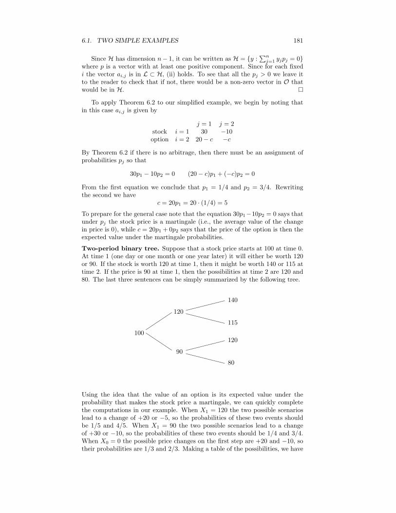
6.1. TWO SIMPLE EXAMPLES 181
Since H has dimension n− 1, it can be written as H = y :∑n
j=1 yjpj = 0where p is a vector with at least one positive component. Since for each fixedi the vector ai,j is in L ⊂ H, (ii) holds. To see that all the pj > 0 we leave itto the reader to check that if not, there would be a non-zero vector in O thatwould be in H.
To apply Theorem 6.2 to our simplified example, we begin by noting thatin this case ai,j is given by
j = 1 j = 2stock i = 1 30 −10option i = 2 20− c −c
By Theorem 6.2 if there is no arbitrage, then there must be an assignment ofprobabilities pj so that
30p1 − 10p2 = 0 (20− c)p1 + (−c)p2 = 0
From the first equation we conclude that p1 = 1/4 and p2 = 3/4. Rewritingthe second we have
c = 20p1 = 20 · (1/4) = 5
To prepare for the general case note that the equation 30p1−10p2 = 0 says thatunder pj the stock price is a martingale (i.e., the average value of the changein price is 0), while c = 20p1 + 0p2 says that the price of the option is then theexpected value under the martingale probabilities.
Two-period binary tree. Suppose that a stock price starts at 100 at time 0.At time 1 (one day or one month or one year later) it will either be worth 120or 90. If the stock is worth 120 at time 1, then it might be worth 140 or 115 attime 2. If the price is 90 at time 1, then the possibilities at time 2 are 120 and80. The last three sentences can be simply summarized by the following tree.
100
QQQQ
120
XXXXXX
140
115
90
XXXXXX
120
80
Using the idea that the value of an option is its expected value under theprobability that makes the stock price a martingale, we can quickly completethe computations in our example. When X1 = 120 the two possible scenarioslead to a change of +20 or −5, so the probabilities of these two events shouldbe 1/5 and 4/5. When X1 = 90 the two possible scenarios lead to a changeof +30 or −10, so the probabilities of these two events should be 1/4 and 3/4.When X0 = 0 the possible price changes on the first step are +20 and −10, sotheir probabilities are 1/3 and 2/3. Making a table of the possibilities, we have

182 CHAPTER 6. MATHEMATICAL FINANCE
X1 X2 probability (X2 − 100)+
120 140 (1/3) · (1/5) 40120 115 (1/3) · (4/5) 1590 120 (2/3) · (1/4) 2090 80 (2/3) · (3/4) 0
so the value of the option is
115· 40 +
415· 15 +
16· 20 =
80 + 120 + 10030
= 10
The last derivation may seem a little devious, so we will now give a secondderivation of the price of the option based on absence of arbitrage. In thescenario described above, our investor has four possible actions:
A0. Put $1 in the bank and end up with $1 in all possible scenarios.
A1. Buy one share of stock at time 0 and sell it at time 1.
A2. Buy one share at time 1 if the stock is at 120, and sell it at time 2.
A3. Buy one share at time 1 if the stock is at 90, and sell it at time 2.
These actions produce the following payoffs in the indicated outcomes
X1 X2 A0 A1 A2 A3 option120 140 1 20 20 0 40120 115 1 20 −5 0 1590 120 1 −10 0 30 2090 80 1 −10 0 −10 0
Noting that the payoffs from the four actions are themselves vectors in four-dimensional space, it is natural to think that by using a linear combination ofthese actions we can reproduce the option exactly. To find the coefficients zi
for the actions Ai we write four equations in four unknowns,
z0 + 20z1 + 20z2 = 40z0 + 20z1 − 5z2 = 15z0 − 10z1 + 30z3 = 20z0 − 10z1 − 10z3 = 0
Subtracting the second equation from the first and the fourth from the thirdgives 25z2 = 25 and 40z3 = 20 so z2 = 1 and z3 = 1/2. Plugging in thesevalues, we have two equations in two unknowns:
z0 + 20z1 = 20 z0 − 10z1 = 5
Taking differences, we conclude 30z1 = 15, so z1 = 1/2 and z0 = 10.The reader may have already noticed that z0 = 10 is the option price. This
is no accident. What we have shown is that with $10 cash we can buy andsell shares of stock to produce the outcome of the option in all cases. In theterminology of Wall Street, z1 = 1/2, z2 = 1, z3 = 1/2 is a hedging strategythat allows us to replicate the option. Once we can do this it follows thatthe fair price must be $10. To do this note that if we could sell it for $12 thenwe can take $10 of the cash to replicate the option and have a sure profit of $2.

6.2. BINOMIAL MODEL 183
6.2 Binomial Model
In this section we consider the Binomial model in which at each time the stockprice the stock is multiplied by u (for ‘up’). or multiplied by d (for ‘down’). Asin the previous section we begin with the
One period case
There are two possible outcomes for the stock called heads (H) and tails (T ).
S0
XXXXXX
S1(H) = S0u
S1(T ) = S0d
We assume that there is an interest rate r, which means that $1 at time 0 isthe same as $(1 + r) at time 1. For the model to be sensible, we need
0 < d < 1 + r < u. (6.1)
Consider now an option that pays off V1(H) or V1(T ) at time 1. This couldbe a call option (S1 −K)+, a put (K − S1)+, or something more exotic, so wewill consider the general case. To find the “no arbitrage price” of this optionwe suppose we have V0 in cash and ∆0 shares of the stock at time 0, and wantto pick these to match the option price exactly:
V0 + ∆0
(1
1 + rS1(H)− S0
)=
11 + r
V1(H) (6.2)
V0 + ∆0
(1
1 + rS1(T )− S0
)=
11 + r
V1(T ) (6.3)
Notice that here we have to discount money at time 1 (i.e., divide it by 1 + r)to make it comparable to dollars at time 0.
To find the values of V0 and ∆0 we define the risk neutral probability p∗ sothat
11 + r
(p∗S0u + (1− p∗)S0d) = S0 (6.4)
Solving we have
p∗ =1 + r − d
u− d1− p∗ =
u− (1 + r)u− d
(6.5)
The conditions in (6.1) imply 0 < p∗ < 1.Taking p∗(6.2) + (1− p∗)(6.3) and using (6.4) we have
V0 =1
1 + r(p∗V1(H) + (1− p∗)V1(T )) (6.6)
i.e., the value is the discounted expected value under the risk neutral probabil-ities. Taking the difference (6.2)− (6.3) we have
∆0
(1
1 + r(S1(H)− S1(T ))
)=
11 + r
(V1(H)− V1(T ))

184 CHAPTER 6. MATHEMATICAL FINANCE
which implies that
∆0 =V1(H)− V1(T )S1(H)− S1(T )
(6.7)
To explain the notion of hedging we consider a concrete example.
Example 6.1. A stock is selling at $60 today. A month from now it will eitherbe at $80 or $50, i.e., u = 4/3 and d = 5/6. We assume an interest rate ofr = 1/18 so the risk neutral probability is
19/18− 5/64/3− 5/6
=49
Consider now a call option (S1 − 65)+. By 6.6) the value is
V0 =1819· 49· 15 =
12019
= 6.3158
Being a savy businessman you offer to sell this for $6.50. You are delightedwhen a customer purchases 10,000 calls for $65,000, but then become worriedabout the fact that if the stock goes up you will lose $85,000. By (6.7) thehedge ratio
∆0 =1530
= 1/2
so you borrow $300,000 - $65,000 = $235,000 and buy 5,000 shares of stock.
Case 1. The stock goes up to $80. Your stock is worth $400,000. You have topay $150,000 for the calls and (19/18)$235,000 = $248,055 to redeem the loanso you make $1,945 (in time 1 dollars).
Case 2. The stock drops to $50. Your stock is worth $250,000. You owe nothingfor the calls but have to pay $248,055 to redeem the loan so again you make$1,945.
The equality of the profits in the two cases may look like a miracle but it is not.By buying the correct amount of stock you replicated the option. This meansyou made a sure profit of the $1,842 difference (in time 0 dollars) between theselling price and fair price of the option, which translates into $1,945 time 1dollars.
N period model
To solve the problem in general we work backwards from the end, repeatedlyapplying the solution of the one period problems. Let a be a string of H’s andT ’s of length n− 1 which represents the outcome of the first n− 1 events. Thevalue of the option at time n after the events in a have occurred, Vn(a), and theamount of stock we need to hold in this situation, ∆n(a), in order to replicatethe option payoff satisfy:
Vn(a) + ∆n(a)(
11 + r
Sn+1(aH)− Sn(a))
=1
1 + rVn+1(aH) (6.8)
Vn(a) + ∆n(a)(
11 + r
Sn+1(aT )− Sn(a))
=1
1 + rVn+1(aT ) (6.9)

6.2. BINOMIAL MODEL 185
Define the risk neutral probability p∗n(a) so that
Sn(a) =1
1 + r[p∗n(a)Sn+1(aH) + (1− p∗n(a))Sn+1(aT )] (6.10)
A little algebra shows that
p∗n(a) =(1 + r)Sn(a)− Sn+1(aT )Sn+1(aH)− Sn+1(aT )
(6.11)
In the binomial model one has p∗n(a) = (1 + r − d)/(u − d). However, stockprices are not supposed to follow the binomial model, but are subject only tothe no arbitrage restriction that 0 < p∗n(a) < 1. Notice that these probabilitiesdepend on the time n and the history a.
Taking p∗n(a)(6.8) + (1− p∗n(a))(6.9) and using (6.10) we have
Vn(a) =1
1 + r[p∗n(a)Vn+1(aH) + (1− p∗n(a))Vn+1(aT )] (6.12)
i.e., the value is the discounted expected value under the risk neutral probabil-ities. Taking the difference (6.8)− (6.9) we have
∆n(a)(
11 + r
(Sn+1(aH)− Sn+1(aT )))
=1
1 + r(Vn+1(aH)− Vn+1(aT ))
which implies that
∆n(a) =Vn+1(aH)− Vn+1(aT )Sn+1(aH)− Sn+1(aT )
(6.13)
In words, ∆n(a) is the ratio of the change in price of the option to the changein price of the stock. Thus for a call or put |∆n(a)| ≤ 1.
The option prices we have defined were motivated by the idea that by tradingin the stock we could replicate the option exactly and hence they are the onlyprice consistent with the absence of arbitrage. We will now go through thealgebra needed to demonstrate this for the general n period model. Supposewe start with W0 dollars and hold ∆n(a) shares of stock between time n andn + 1 when the otucome of the first n events is a. If we invest the money notin the stock in the money market account which pays interest r per period ourwealth satisfies the recursion:
Wn+1 = ∆nSn+1 + (1 + r)(Wn −∆nSn) (6.14)
Theorem 6.3. If W0 = V0 and we use the investment strategy in (6.13) thenwe have Wn = Vn.
In words, we have a trading strategy that replicates the option payoffs.
Proof. We proceed by induction. By assumption the result is true when n = 0.Let a be a string of H and T of length n. (6.14) implies
Wn+1(aH) = ∆n(a)Sn+1(aH) + (1 + r)(Wn(a)−∆n(a)Sn(a))= (1 + r)Wn(a) + ∆n(a)[Sn+1 − (1 + r)Sn(a)]
By induction the first term = (1 + r)Vn(a). Letting q∗n(a) = 1 − p∗n(a), (6.10)implies
(1 + r)Sn(a) = p∗n(a)Sn+1(aH) + q∗n(a)Sn+1(aT )

186 CHAPTER 6. MATHEMATICAL FINANCE
Subtracting this equation from Sn+1(aH) = Sn+1(aH) we have
Sn+1(aH)− (1 + r)Sn(a) = q∗n(a)[Sn+1(aH)− Sn+1(aT )]
Using (6.13) now, we have
∆n(a)[Sn+1 − (1 + r)Sn(a)] = q∗n(a)[Vn(aH)− Vn+1(aT )]
Combining our results then using (6.12)
Wn+1(aH) = (1 + r)Vn(a) + q∗n(a)[Vn(aH)− Vn+1(aT )]= p∗n(a)Vn(aH) + q∗nVn(aT ) + q∗n(a)[Vn(aH)− Vn+1(aT )]= Vn+1(aH)
The proof that Wn+1(aT ) = Vn+1(aT ) is almost identical.
Our next goal is to prove that the value of the option is its expected valueunder the risk neutral probability discounted by the interest rate (Theorem6.5). The first step is:
Theorem 6.4. In the binomial model, under the risk neutral probability mea-sure Mn = Sn/(1 + r)n is a martingale with respect to Sn.
Proof. Let p∗ and 1 − p∗ be defined by (6.5). Given a string a of heads andtails of length n
P ∗(a) = (p∗)H(a)(1− p∗)T (a)
where H(a) and T (a) are the number of heads and tails in a. To check themartingale property we need to show that
E∗(
Sn+1
(1 + r)n+1
∣∣∣∣Sn = sn, . . . S0 = s0
)=
Sn
(1 + r)n
where E∗ indicates expected value with respect to P ∗. Letting Xn+1 = Sn+1/Sn
which is independent of Sn and is u with probability p∗ and d with probability1− p∗ we have
E∗(
Sn+1
(1 + r)n+1
∣∣∣∣Sn = sn, . . . S0 = s0
)=
Sn
(1 + r)nE∗(
Xn+1
1 + r
∣∣∣∣Sn = sn, . . . S0 = s0
)=
Sn
(1 + r)n
since E∗Xn+1 = 1 + r by (6.10).
Notation. To make it easier to write computations like the last one we will let
En(Y ) = E(Y |Sn = sn, . . . S0 = s0) (6.15)
or in words, the conditional expectation of Y given the information at time n.
A second important martingale result is
Theorem 6.5. Assume that the holdings ∆n(a) can be determined from theoutcomes of the first n stock movements and let Wn be the wealth process definedby (6.14). Under P ∗, Wn/(1 + r)n is a martingale, and hence the value hasV0 = E∗(Vn/(1 + r)n).

6.3. CONCRETE EXAMPLES 187
Proof. The second conclusion follows from the first and Theorem 6.3. A littlearithmetic with (6.14) shows that
Wn+1
(1 + r)n+1=
Wn
(1 + r)n+ ∆n
(Sn+1
(1 + r)n+1− Sn
(1 + r)n
)
Since ∆n(a) is an admissible gambling strategy and Sn/(1+r)n is a martingale,the desired result follows from Theorem 5.12.
6.3 Concrete Examples
Turning to examples, we will often use the following binomial model because itleads to easy arithmetic
u = 2, d = 1/2, r = 1/4 (6.16)
The risk neutral probabilities
p∗ =1 + r − d
u− d=
5/4− 1/22− 1/2
=12
and by (6.12) the option prices follow the recursion:
Vn(a) = .4[Vn+1(aH) + Vn+1(aT )] (6.17)
Example 6.2. Callback options. In this option you can buy the stock attime 3 at its current price and then sell it at the highest price seen in the pastfor a profit of
V3 = max0≤m≤3
Sm − S3
Our goal is to compute the value Vn(a) and the replicating strategy ∆n(a) forthis option in the binomial model given in (6.16) with S0 = 4. Here the numbersabove the nodes are the stock price, while those below are the values of Vn(a)and ∆n(a). Starting at the right edge, S3(HTT ) = 2 but the maximum in thepast is 8 = S1(H) so V3(HTT ) = 8− 2 = 6.

188 CHAPTER 6. MATHEMATICAL FINANCE
XXXXXX
XXXXXX
XXXXXX
XXXXXX
HHHHHH
HHHHHH
@@@@@@
32
8
8
2
8
2
2
.5
0
8
0
6
0
2
2
3.5
16
4
4
1
3.2
2.4
0.8
2.2
−.25
−1
−.333
−1
8
2
2.24
1.2
.0666
−.466
4
1.376.1733
On the tree, stock prices are above the nodes and option prices below. Toexplain the computation of the option price note that by (6.17).
V2(HH) = 0.4(V3(HHH) + V3(HHT )) = 0.4(0 + 8) = 3.2V2(HT ) = 0.4(V3(HTH) + V3(HTT )) = 0.4(0 + 6) = 2.4
V1(H) = 0.4(V2(HH) + V2(HT )) = 0.4(3.2 + 2.4) = 2.24
If one only wants the option price then Theorem 6.5 which says that V0 =E∗(VN/(1 + r)N ) is much quicker:
V0 = (4/5)3 · 18· [0 + 8 + 0 + 6 + 0 + 2 + 2 + 2 + 3.5] = 1.376
Example 6.3. Put option. We will use the binomial model in (6.16) butnow suppose S0 = 8 and consider the put option with value V3 = (10 − S3)+.The value of this option depends only on the price so we can reduce the treeconsidered above to:
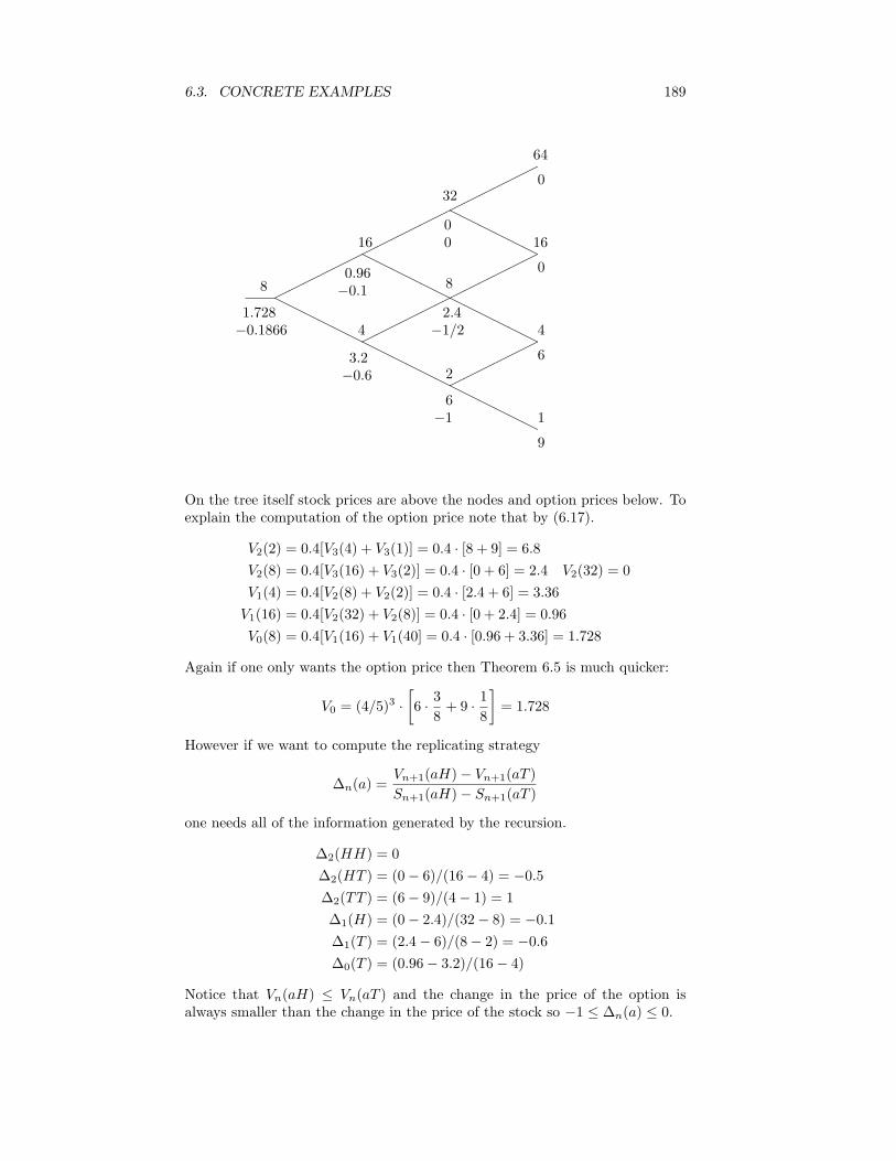
6.3. CONCRETE EXAMPLES 189
HHHHHHHHHHHHHHHHHH
HHHHHHHHHHHH
HHHHHH
64
16
4
1
0
0
6
9
32
8
2
0
2.4
6
0
−1/2
−1
16
4
0.96
3.2
−0.1
−0.6
8
1.728−0.1866
On the tree itself stock prices are above the nodes and option prices below. Toexplain the computation of the option price note that by (6.17).
V2(2) = 0.4[V3(4) + V3(1)] = 0.4 · [8 + 9] = 6.8V2(8) = 0.4[V3(16) + V3(2)] = 0.4 · [0 + 6] = 2.4 V2(32) = 0V1(4) = 0.4[V2(8) + V2(2)] = 0.4 · [2.4 + 6] = 3.36
V1(16) = 0.4[V2(32) + V2(8)] = 0.4 · [0 + 2.4] = 0.96V0(8) = 0.4[V1(16) + V1(40] = 0.4 · [0.96 + 3.36] = 1.728
Again if one only wants the option price then Theorem 6.5 is much quicker:
V0 = (4/5)3 ·[6 · 3
8+ 9 · 1
8
]= 1.728
However if we want to compute the replicating strategy
∆n(a) =Vn+1(aH)− Vn+1(aT )Sn+1(aH)− Sn+1(aT )
one needs all of the information generated by the recursion.
∆2(HH) = 0∆2(HT ) = (0− 6)/(16− 4) = −0.5∆2(TT ) = (6− 9)/(4− 1) = 1∆1(H) = (0− 2.4)/(32− 8) = −0.1∆1(T ) = (2.4− 6)/(8− 2) = −0.6∆0(T ) = (0.96− 3.2)/(16− 4)
Notice that Vn(aH) ≤ Vn(aT ) and the change in the price of the option isalways smaller than the change in the price of the stock so −1 ≤ ∆n(a) ≤ 0.

190 CHAPTER 6. MATHEMATICAL FINANCE
Example 6.4. Put-call parity. Consider the binomial model with S0 = 32,u = 3/2, d = 2/3 and r = 1/6. By (6.5) the risk neutral probability
p∗ =1 + r − d
u− d=
7/6− 2/33/2− 2/3
=3/65/6
= 0.6
so by (6.12) the value satisfies
Vn(a) =17(3.6Vn+1(aH) + 2.4Vn+1(aT ))
We will now compute the values for the call and put with strike 49 and expiry2. In the diagrams below the numbers above the line are the value of the stockand the ones below are the value of the option, and the replicating strategy.
AAA
AAA
AAA
81
call 32
36
0
16
0
54
115.27
24
0
36
414.7249
AAA
AAA
AAA
81
put 0
36
13
16
33
54
31.27
24
1267
36
414.7249
We have written the values as fractions to make it clear that the value attime 0 of these two options are exactly the same. Once you realize this it iseasy to prove.
Theorem 6.6. The values VP and VC of the put and call options with the samestrike K and expiration N are related by
VP − VC =K
(1 + r)N− S0
In particular if K = (1 + r)NS0 then VP = VC .
Proof. The key observation is that
SN + (K − SN )+ − (SN −K)+ = K
Consider the two cases SN ≥ K and SN ≤ K. Dividing by (1 + r)N , taking E∗
expected value and using the fact that Sn/(1 + r)n is a martingale
S0 + E∗ (K − SN )+
(1 + r)N− E∗ (K − SN )+
(1 + r)N=
K
(1 + r)N
Since the second term on the left is VP and the third is VC the desired resultfollows.

6.4. CAPITAL ASSET PRICING MODEL 191
It is important to note that the last result can be used to compute the valueof any put from the corresponding call. Returning to the previous example andlooking at the time 1 node where the price is 54, the formula above says
31.27− 115.2
7=
847
= 12 =6749− 54
Example 6.5. Knockout options. In these options when the price fallsbelow a certain level the option is worthless no matter what the value of thestock is at the end. To illustrate consider the binomial model from Example6.4: u = 3/2, d = 2/3, and r = 1/6. This time we suppose S0−24 and considera call (S3 − 28)+ with a knockout barrier at 20, that is if the stock price dropsbelow 20 the option becomes worthless. As we have computed the risk neutralprobability is p∗ = 0.6 and the value recursion is
Vn(a) =67[.6Vn(aH) + .4Vn(aT )],
with the extra boundary condition that if the price is ≤ 20 the value is 0.
HHHHHH
HHHHHHHHH
HHH
HHHHHH
81
36
16
53
8
0
54
24
30
4.114
36
16
16.839
0
24
8.660
To check the answer note that the knockout feature eliminates one of the pathsto 36 so
V0 = (6/7)3[(.6)3 · 53 + 2(.6)2(.4) · 8] = 8.660
From this we see that the knockout barrier reduced the value of the option by(6/7)3(0.6)2(0.4) · 8 = 0.7255.
6.4 Capital Asset Pricing Model
In this section, we will explore an approach to option pricing which is morein keeping with traditional economic thinking. Our hidden agenda here is toshow how ideas from Section 6.2 can be used to simplify a complicated lookingproblem.
Each investor is assumed to have a utility function that nondecreasing andconcave. If 0 ≤ λ ≤ 1 and x < y then
U(λx + (1− λ)y) ≥ λU(x) + (1− λ)U(y) (6.18)

192 CHAPTER 6. MATHEMATICAL FINANCE
1.5
2
2.5
3
3.5
0
0.5
1
0 5 10 15 20 25
Geometrically, the line segment from (x,U(x)) to (y, U(y)) lies below the graphof the function.
In economic terms investors are risk averse. They prefer a sure pay-off ofλx+(1−λ)y to a lottery ticket that pays x with probability λ and pays y withprobability 1− λ.
Lemma 6.7. If U is smooth then U is concave if U ′′ ≤ 0.
Proof. U ′′ ≤ 0 implies that the U ′ is decreasing, so if x > y
1λ(x− y)
∫ λx+(1−λ)y
y
U ′(z) dz ≥ 1x− y
∫ x
y
U ′(z) dz
In words, the average slope over [y, λx+(1−λ)y], and intervalof length λ(x−y)is larger than that over [y, x]. Doing the integrals and a little algebra gives
U(λx + (1− λy))− U(y) ≥ λ(U(x)− U(y))
which after a little more algebra is (6.18).
Some concrete examples of utility functions are:
Up(x) = xp/p with 0 < p < 1 for x ≥ 0 and U(x) = −∞ for x < 0.
U0(x) = lnx for x > 0 and U(x) = −∞ for x ≤ 0.
Up(x) = xp/p with p < 0 for x ≥ 0 and U(x) = −∞ for x ≤ 0.
Dividing by p is useful here because in all three cases U ′p(x) = xp−1 and U ′′
p (x) =(p− 1)xp−2 ≤ 0 for x ≥ 0. The second half of the definition is forced on us. Inthe second and third cases Up(x)→ −∞ as x ↓ 0, while in the first U ′
p(x)→ +∞as x ↓ 0.
An optimal investment problem. Given a utility function U and aninitial wealth, find an admissible trading strategy ∆n to maximize EU(WN ),where the wealth Wn satisfies the recursion (6.14)
Wn+1 = ∆nSn+1 + (1 + r)(Wn −∆nSn)
Example 6.6. Consider now the concrete example of maximizing U(x) = lnxfor a two-period binomial model with S0 = 4, u = 2, d = 1/2, and r = 1/4where the probability of up and down are 2/3 and 1/3 respectively. Note thatwe are optimizing under the real world or physical measure rather than the risk

6.4. CAPITAL ASSET PRICING MODEL 193
neutral probabilities p∗ = q∗ = 1/2 which are a fiction used to compute optionprices.
Our wealth at time 1 satisfies
W1(H) = 8∆0 +54(W0 − 4∆0) =
54W0 + 3∆0
W1(T ) = 2∆0 +54(W0 − 4∆0) =
54W0 + 3∆0
Writing δ1 = ∆1(H), δ2 = ∆1(T ), and δ0 = ∆0 our wealth at time 2 is
W2(HH) = 16δ1 +54(W1(H)− 8δ1) = 6δ1 +
154
δ0 +2516
W0
W2(HT ) = 4δ1 +54(W1(H)− 8δ1) = −6δ1 +
154
δ0 +2516
W0
W2(TH) = 4δ2 +54(W1(H)− 2δ2) =
32δ2 −
154
δ0 +2516
W0
W2(TT ) = δ2 +54(W1(H)− 2δ2) = −3
2δ2 −
154
δ0 +2516
W0
Let y0, y1, y2, and y3 be our wealth at time 2 under outcomes HH, HT , TH,and TT . To see the correspondence think of binary digits H = 0 and T = 1.With this notation we want to maximize
V = E lnW2 =49
ln y0 +29
ln y1 +29
ln y2 +19
ln y3
Differentiating and using the formulas for the yi we have
∂V
∂δ0=
154
(49· 1y0
+29· 1y1− 2
9· 1y2− 1
9· 1y3
)∂V
∂δ1= 6
(49· 1y0− 2
9· 1y1
)∂V
∂δ2=
32
(29· 1y2− 1
9· 1y3
)The second and third equations imply that 2y1 = y0 and 2y3 = y2. The firstequation implies
4y0
+2y1
=2y2
+1y3
or 4/y1 = 2/y3, i.e., 2y3 = y1. Thus if y3 = c, y1 = y2 = 2c, and y3 = 4c.Adding the equations for the W2 we have
9c = y0 + y1 + y2 + y3 =254
W0
and it follows that
y3 =49· 25
4W0 y2 = y1 =
29· 25
4W0 y0 =
19· 25
4W0 (6.19)
Once we have the yi’s we have
y0 − y1 = 12δ1 y2 − y3 = 3δ2 y0 + y1 − y2 − y3 = 15δ0

194 CHAPTER 6. MATHEMATICAL FINANCE
Turing to the two=period case for a general binomial model, the previouscalculation suggests that what we really want to solve for are the terminalvalues yi. We cannot achieve any yi. Theorem 6.5 implies that our discountedwealth Wn/(1 + r)n is a martingale under P ∗, so letting p∗m be the risk neutralprobabilities of outcomes m = 0, 1, 2, 3, we must have
1(1 + r)2
3∑m=0
p∗mym = W0
Conversely, given a vector that satisfies the last condition, the option with thesepayoffs has value W0 and there is a trading strategy that allows us to replicatethe option. Letting pm be the physical probabilities of outcomes m = 0, 1, 2, 3,our problem m is to
Maximize∑3
m=0 pm ln ym subject to (1 + r)−2∑3
m=0 p∗mym = W0.
Consider the unconstrained optimization problem of maximizing
L =3∑
m=0
pmU(ym)− λ
(1 + r)2
(3∑
m=0
p∗mym −W0(1 + r)2)
Differentiating we have∂L
∂ym=
pm
ym− λp∗m
(1 + r)2
Setting these equal to 0 we have
ym =pm(1 + r)2
λp∗m
The final detail is to pick λ to satisfy the constraint, i.e.,
(1 + r)2
λ
3∑m=0
pm = W0
or since the pm sum to 1, λ = 1/W0 and
ym = W0(1 + r)2pm
p∗m
Since 1 + r = 5/4, p3 = 4/9, p2 = p1 = 2/9, p0 = 1/9, and all the p∗m = 1/4this agrees with (6.19). However from the new solution we can easily see thenature of the solution in general.
6.5 American Options
European option contracts specify an expiration date, and if the option is to beexercised at all, this must occur at the expiration date. An option whose ownercan choose to exercise it at any time is called an American option. We willmostly be concerned with call and put options where the value at exercise is afunction of the stock price, but it is no more difficult to consider path dependentoptions, so we derive the basic formulas in that generality.
Given a sequence a of heads and tails of length n let gn(a) be the value ifwe exercise at time n. Our first goal is to compute the value function Vn(a)

6.5. AMERICAN OPTIONS 195
for the N -period problem. To simplify some statements, we will suppose withessentially no loss of generality that gN (a) ≥ 0, so VN (a) = gN (a). To workbackwards in time note that at time n we can exercise the option or let thegame proceed for one more step. Since we will stop or continue depending onwhich choice gives the better payoff:
Vn(a) = max
gn(a),1
1 + r[p∗n(a)Vn+1(aH) + q∗n(a)Vn+1(aT )]
(6.20)
where p∗n(a) and q∗n(a) = 1−p∗n(a) are the risk-neutral probabilities which makethe underlying stock a martingale.
AAA
AAA
AAA
AAA
AAA
AAA
64, 0
16, 0
4, 6
1, 9
32, 0
0, 0*
8, 2.4
2, 2.4*
2, 8
8*, 6
16, 0.96
0, 0.96*
4, 6
6*,4.16
8, 2.874
2, 2.784*
Example 6.7. For a concrete example, suppose as we did in Example 6.3 thatthe stock price follows the binomial model with S0 = 8, u = 2, d = 1/2, r = 1/4and consider a put option with strike 10, that is gn = (10 − sn)+. The riskneutral probability p∗ = 0.5 and the recursion is
Vn−1(a) = 0.4[Vn(aH) + Vn(aT )]
On the drawing above, the two numbers above each line are the price of thestock and the value of the option. Below the line are the value of the option ifexercised, and the value computed by the recursion if we continue for one moreperiod. A star indicates the large of the two, which is the value of the option atthat time. To explain the solution, note that working backwards from the end.
V2(2) = max8, 0.4(6 + 9) = 6 = 8V2(8) = max2, 0.4(0 + 6) = 2.4 = 2.4
V2(32) = max0, 0 = 0V1(4) = max6, 0.4(2.4 + 8) = 4.16 = 6
V1(16) = max0, 0.4(0 + 2.4) = 0.96 = 0.96V0(8) = max2, 0.4(0.96 + 6) = 2.784 = 2.784

196 CHAPTER 6. MATHEMATICAL FINANCE
This computes the value and the optimal strategy: stop or continue at each nodedepending on which value is larger. Notice that this is larger than the value1.728 we computed for the European version. It certainly cannot be strictlyless since one possibility in the American option is to continue each time andthis turns it into a European option.
For some of the theoretical results it is useful to notice that
V0 = maxτ
E∗(
gτ
(1 + r)τ
)(6.21)
where the maximum is taken over all stopping times τ with 0 ≤ τ ≤ N . InExample 6.7 τ(T ) = 1 and τ(H) = 3, i.e., if the stock goes down on the firststep we stop. Otherwise we continue until the end.
V0 =12· 6 · 4
5+
18· 6 ·
(45
)3
= 2.4 + 0.384
Proof. The key to prove the stronger statement
Vn(a) = maxτ≥n
E∗n(gτ/(1 + r)τ−n)
where E∗n is the conditional expectation given the events that have occurred up
to time n. Let Wn(a) denote the right-hand side. If we condition on the first noutcomes being a then P (τ = n) is 1 or 0. In the first case we get gn(a). In thesecond case Wn(a) = [p∗n(a)Wn+1(aH) + q∗n(a)Wn+1(aT )]/(1 + r), so Wn andVn satisfy the same recursion.
Example 6.8. Continue now the set-up of the previous example but considerthe call option (Sn − 10)+. The computations are the same but the result isboring: the optimal strategy is to always continue, so there is no differencebetween the American and the European option.
AAA
AAA
AAA
AAA
AAA
AAA
64, 54
16, 6
4, 0
1, 0
32, 24
22, 24*
8, 2.4
0, 2.4*
2, 0
0, 0*
16, 10.56
6, 10.56*
4, 0.96
0, 0.96*
8, 4.608
0, 4.608*

6.5. AMERICAN OPTIONS 197
To spare the reader the chore of doing the arithmetic we give the recursion:
V2(2) = max0, 0 = 0V2(8) = max0, 0.4(0 + 6) = 2.4 = 2.4
V2(32) = max22, 0.4(54 + 60 = 24 = 24V1(4) = max0, 0.4(0 + 2.4) = 0.96 = 0.96
V1(16) = max6, 0.4(24 + 2.4) = 10.56 = 10.56V0(8) = max0, 0.4(10.56 + 0.96) = 4.608 = 4.608
Our next goal is to prove that it is always optimal to continue in the caseof the American call option. To explain the reason for this we formulate anabstract result. We say that g is convex if whenever 0λ ≤ 1 and s1, s2 are realnumbers
g(λs1 + (1− λ)s2) ≤ λg(s1) + (1− λ)g(s2) (6.22)
Geometrically the line segment from (s1, g1(s)) to (s2, g2(s)) always lies abovethe graph of the function g. This is true for the call g(x) = (x−K)+ and theput g(x) = (K−x)+. However only the call satisfies all of the conditions in thefollowing result.
Theorem 6.8. If g is a nonnegative convex function with g(0) = 0 then forthe American option with payoff g(Sn) it is optimal to wait until the end toexercise.
Proof. Since Sn/(1 + r)n is a martingale under P ∗
g(Sn) = g
(E∗
n
(Sn+1
1 + r
))Under the risk neutral probability
Sn(a) = p∗n(a)Sn+1(aH)
1 + r+ (1− p∗n(a))
Sn+1(aH)1 + r
Using (6.22) with λ = p∗n(a) it follows that
g
(E∗
n
(Sn+1
1 + r
))≤ E∗
n
(g
(Sn+1
1 + r
))Using (6.22) with s2 = 0 and g(0) = 0 we have g(λs1) ≤ λg(s1), so we have
E∗n
(g
(Sn+1
1 + r
))≤ 1
1 + rE∗
ng(Sn+1)
Combining three of the last four equations we have
g(Sn) ≤ 11 + r
E∗ng(Sn+1)
This shows that if we were to stop at time n for some outcome a, it would bebetter to continue. Using (6.21) now the desired result follows.
198 CHAPTER 6. MATHEMATICAL FINANCE
6.6 Black-Scholes formula
Many options take place over a time period of one or more months, so it isnatural consider St to be the stock price after t years. We could use a binomialmodel in which prices change at the end of each day but it would also benatural to update prices several times during the day. Let h be the amount oftime measured in years between updates of the stock price. This h will be verysmall e.g., 1/365 for daily updates so it is natural to let h→ 0. Knowing whatwill happen when we take the limit we will let
Snh = S(n−1)h exp(µh + σ√
hXn)
where P (Xn = 1) = P (Xn = −1) = 1/2. This is binomial model with
u = exp(µh + σ√
h) d = exp(µh− σ√
h) (6.23)
Iterating we see that
Snh = S0 exp
(µnh + σ
√h
n∑m=1
Xm
)(6.24)
If we let t = nh the first term is just µt. Writing h = t/n the second termbecomes
σ√
t · 1√n
n∑m=1
Xm
To take the limit as n→∞, we use the
Theorem 6.9. Central Limit Theorem. Let X1, X2, . . . be i.i.d. with EXi =0 and var (Xi) = 1 Then for all x we have
P
(1√n
n∑m=1
Xm ≤ x
)→ P (χ ≤ x) (6.25)
where χ has a standard normal distribution. That is,
P (χ ≤ x) =∫ x
−∞
1√2π
e−y2/2 dy
The conclusion in (6.25) is often written as
1√n
n∑m=1
Xm ⇒ χ
where ⇒ is read “converges in distribution to.” Recalling that if we multiplya standard normal χ by a constant c then the result has a normal distributionwith mean 0 and variance σ2, we see that
√t · 1√
n
n∑m=1
Xm ⇒√
tχ
and the limit is a normal with mean 0 and variance t.This motivates the following definition:

6.6. BLACK-SCHOLES FORMULA 199
Definition. B(t) is a standard Brownian motion if B(0) = 0 and it satisfiesthe following conditions:
(a) Independent increments. Whenever 0 = t0 < t1 < . . . < tk
B(t1)−B(t0), . . . , B(tk)−B(tk−1) are independent.
(b) Stationary increments. The distribution of Bt −Bs is normal (0, t− s).
(c) t→ Bt is continuous.
To explain (a) note that if ni = ti/h then the sums∑ni−1<m≤ni
Xm i = 1, . . . k
are independent. For (b) we note that that the distribution of the sum onlydepends on the number of terms and use the previous calculation. Condition (c)is a natural assumption for the physical system which motivated this definition:the erratic movement of a pollen grain in water as seen under a microscope byBrown in 1825.
Using the new definition, our stock price model can be written as
St = S0 · exp(µt + σBt) (6.26)
where Bt is a standard Brownian motion Here µ is the exponential growthrate of the stock, and σ is its volatility. If we also assume that the per periodinterest rate in the approximating model is rh, and recall that(
11 + rh
)t/h
=1
(1 + rh)t/h→ 1
ert= e−rt
then the discounted stock price is
e−rtSt = S0 · exp((µ− r)t + σBt)
By the formula for the moment generating function for the normal withmean 0 and variance σ2t, see (5.15),
E exp(−(σ2/2)t + σBt) = 1
Since Bt has independent increments, if we let
µ = r − σ2/2 (6.27)
then reasoning as for the exponential martingale, Example 5.6, the discountedstock price, e−rtSt is a martingale.
Extrapolating wildly from discrete time, we can guess that the option priceis its expected value after changing the probabilities to make the stock price amartingale.
Theorem 6.10. Write E∗ for expected values when µ = r − σ2/2 in (6.26).The value of a European option g(ST ) is given by E∗e−rT g(ST ).

200 CHAPTER 6. MATHEMATICAL FINANCE
Proof. We prove this by taking limits of the discrete approximation. The riskneutral probabilities, p∗h, are given by
p∗h =1 + rh− d
u− d. (6.28)
Using the formulas for u and d in (6.23 and recalling that ex = 1+x+x2/2+· · · ,
u = 1 + µh + σ√
h +12(µh + σ
√h)2 + . . .
= 1 + σ√
h + (σ2/2 + µ)h + . . . (6.29)
d = 1 + µh− σ√
h + (σ2/2 + µ)h + . . .
so from (6.28) we have
p∗h ≈σ√
h + (r − µ− σ2/2)h2σ√
h=
12
+r − µ− σ2/2
2σ
√h
If Xh1 , Xh
2 , . . . are i.i.d. with
P (Xh1 = 1) = p∗h P (Xh
1 = −1) = 1− p∗h
then the mean and variance are
EXhi = 2p∗h =
(r − µ− σ2/2)σ
√h
var (Xhi ) = 1− (EXh
i )2 → 1
To apply the central limit theorem we note that
σ√
h
t/h∑m=1
Xhm = σ
√h
t/h∑m=1
(Xhm − EXh
m) + σ√
h
t/h∑m=1
EXhm
→ σBt + (r − µ + σ2/2)t
so under the risk neutral measure, P ∗,
St = S0 · exp((r − σ2/2)t + σBt)
The value of the option g(ST ) in the discrete approximation is given by theexpected value under its risk neutral measure. Ignoring the detail of provingthat the limit of expected values is the expected value of the limit, we haveproved the desired result.
The Black-Scholes partial differential equation
We continue to suppose that the option payoff at time T is g(ST ). Let V (t, s)be the value of the option at time t < T when the stock price is s. Reasoningwith the discrete time approximation and ignoring the fact that the value inthis case depends on h,
V (t− h, s) =1
1 + rh[p∗V (t, su) + (1− p∗)V (t, sd)]
6.7. CALLS AND PUTS 201
Doing some algebra we have
V (t, s)− (1 + rh)V (t− s, h) = p∗[V (t, s)− V (t, su)]+ (1− p∗)[V (t, s)− V (t, sd)]
Dividing by h we have
V (t, s)− V (t− h, s)h
− rV (t− h, s) (6.30)
= p∗[V (t, s)− V (t, su)
h
]+ (1− p∗)
[V (t, s)− V (t, sd)
h
]Letting h→ 0 the left-hand side of (6.30) converges to
∂V
∂t(t, s)− rV (t, s) (6.31)
Expanding V (t, s) in a power series in s
V (t, s′)− V (t, s) ≈ ∂V
∂x(t, s)(s′ − s) +
∂2V
∂x2(t, s)
(s′ − s)2
2
Using the last equations with s′ = su and s′ = sd, the right-hand side of (6.30)is
≈ ∂V
∂x(t, s)s[(1− u)p∗ + (1− d)(1− p∗)]/h
− 12
∂2V
∂x2(t, s)s2[p∗(1− u)2 + (1− p∗)(1− d)2]/h
From (6.28)
(1− u)p∗ + (1− d)(1− p∗)h
≈ −(
σ2
2+ µ
)= −r
(1− u)2p∗ + (1− d)2(1− p∗)h
≈ σ2
so taking the limit, the right-hand side of (6.30) is
∂V
∂x(t, s)s[−rh] +
12
∂2V
∂x2(t, s)s2σ2h
Combining the last equation with (6.31) and (6.30) we have that the valuefunction satisfies
∂V
∂t− rV (t, s) + rs
∂V
∂x(t, s) +
12σ2s2 ∂2V
∂x2(t, s) = 0 (6.32)
for 0 ≤ t < T with boundary condition V (T, s) = g(s).
6.7 Calls and Puts
We will now apply the theory developed in the previous section to the concreteexamples of calls and puts. At first glance the formula in the first result maylook complicated, but given that the value is defined by soolving a PDE, it isremarkable that such a simple formula exists.

202 CHAPTER 6. MATHEMATICAL FINANCE
Theorem 6.11. The price of the European call option (St −K)+ is given by
S0Φ(d1)− e−rtKΦ(d2)
where the constants
d1 =ln(S0/K) + (r + σ2/2)t
σ√
td2 = d1 − σ
√t.
Proof. Using the fact that log(St/S0) has a normal(µt, σ2t) distribution withµ = r − σ2/2, we see that
E∗(e−rt(St −K)+) = e−rt
∫ ∞
log(K/S0)
(S0ey −K)
1√2πσ2t
e−(y−µt)2/2σ2t dy
Splitting the integral into two and then changing variables y = µt + wσ√
t,dy = σ
√t dw the integral is equal to
= e−rtS0eµt 1√
2π
∫ ∞
α
ewσ√
te−w2/2 dw − e−rtK1√2π
∫ ∞
α
e−w2/2 dw (6.33)
where α = (log(K/S0)− µt)/σ√
t. The handle the first term, we note that
1√2π
∫ ∞
α
ewσ√
te−w2/2 dw = etσ2/2
∫ ∞
α
1√2π
e−(w−σ√
t)2/2 dw
= etσ2/2 P (normal(σ√
t, 1) > α)
The last probability can be written in terms of the distribution function Φ of anormal(0,1) χ, i.e., Φ(t) = P (χ ≤ t), by noting
P (normal(σ√
t, 1) > α) = P (χ > α− σ√
t)
= P (χ ≤ σ√
t− α) = Φ(σ√
t− α)
where in the middle equality we have used the fact that χ and −χ have thesame distribution. Using the last two computations in (6.33) converts it to
e−rtS0eµteσ2t/2Φ(σ
√t− α)− e−rtKΦ(−α)
Now e−rteµteσ2t/2 = 1 since µ = r − σ2/2. As for the argument of the firstnormal
d1 = σ√
t− α =log(S0/K) + (r − σ2/2)t
σ√
t+ σ√
t
which agrees with the formula given in the theorem. The second one is mucheasier to see: d2 = d1 − σ
√t.
Example 6.9. A Google call options. On the morning of December 5,2011 Google stock was selling for $620 a share and a March 12 call option withstrike K = 635 was selling for $33.10. To compare this with the predictionof the Black-Scholes formula we assume an interest rate of r = 0.01 per yearand assume a volatility σ = 0.3. The 100 days until expiration of the optionare t = 0.27393 years. With the help of a little spreadsheet we find that theformula predcits a price of $32.93.

6.8. EXERCISES 203
Example 6.10. Put-call parity allows us to compute the value of the put-option, VP from the value of the call option VC by the formula:
VP − VC = e−rT K − S0
In the example for March 12 Google options, exp(−rt) = 0.9966 so we mightas well ignore that factor. As the next table shows the formula works well inpractice
strike VP VC S0 + VP − VC
600 28.00 55.60 598.20640 45.90 32.70 638.20680 74.16 17.85 681.31
6.8 Exercises
6.1. A stock is now at $110. In a year its price will either be $121 or $99. (a)Assuming that the interest rate is r = 0.04 find the price of a call (S1 − 113)+.(b) How much stock ∆0 do we need to buy to replicate the option. (c) Verifythat having V0 in cash and ∆0 in stock replicates the option exactly.
6.2. A stock is now at $60. In a year its price will either be $75 or $45. (a)Assuming that the interest rate is r = 0.05 find the price of a put (60−S1−)+.(b) How much stock ∆0 do we need to sell to replicate the option. (c) Verifythat having V0 in cash and ∆0 in stock replicates the option exactly.
6.3. It was crucial for our no arbitrage computations that there were only twopossible values of the stock. Suppose that a stock is now at 100, but in onemonth my be at 130, 110 or 80 in outcomes that we call 1, 2 and 3. (a) Find allthe (nonnegative) probabilities p1, p2 and p3 = 1− p1− p2 that make the stockproce a martingale. (b) Find the maximum and minimum values, v1 and v0,of the expected value of the the call option (S1 − 105)+ among the martingaleprobabilities. (c) Show that we can start with v1 in cash, buy x1 shares of stockand we have v1 +x1(S1−S0) ≥ (S1−105)+ in all three outcomes with equalityfor 1 and 3. (d) If we start with v0 in cash, buy x0 shares of stock and we havev0 + x0(S1−S0) ≤ (S1− 105)+ in all three outcomes with equality for 2 and 3.(e) Use (c) and (d) to argue that the only prices for the option consistent withabsence of arbitrage are those in [v0, v1].
6.4. The Cornell hockey team is playing a game against Harvard that it willeither win, lose, or draw. A gambler offers you the following three payoffs, eachfor a $1 bet
win lose drawBet 1 0 1 1.5Bet 2 2 2 0Bet 3 .5 1.5 0
(a) Assume you are able to buy any amounts (even negative) of these bets.Is there an arbitrage opportunity? (b) What if only the first two bets areavailable?
6.5. Suppose Microsoft stock sells for 100 while Netscape sells for 50. Threepossible outcomes of a court case will have the following impact on the twostocks.

204 CHAPTER 6. MATHEMATICAL FINANCE
Microsoft Netscape1 (win) 120 302 (draw) 110 553 (lose) 84 60
What should we be willing to pay for an option to buy Netscape for 50 afterthe court case is over? Answer this question two ways: (i) find a probabilitydistribution so that the two stocks are martingales, (ii) show that by using cashand buying Microsoft and Netscape stock one can replicate the option.
6.6. Consider the two-period binomial model with u = 2, d = 1/2 and interestrate r = 1/4. and suppose S0 = 100. What is the value of the European calloption with strike price 80, i.e., the option with payoff (S2 − 80)+. Find thestock holdings ∆0, ∆1(H) and ∆1(T ) need to replicate the option exactly.
6.7. Consider the two-period binomial model with u = 3/2, d = 2/3, interestrate r = 1/6. and suppose S0 = 45. What is the value of the European calloption with strike price 50, i.e., the option with payoff (50 − S2)+. Find thestock holdings ∆0, ∆1(H) and ∆1(T ) need to replicate the option exactly.
6.8. The payoff of the Asian option is based on the average price: An = (S0 +· · · + Sn)/(n + 1). Suppose that the stock follows the binomial model withS0 = 4, u = 2, d = 1/2, and r = 1/4. (a) Compute the value function Vn(a)and the replicating portfolio ∆n(a) for the three period call option with strike4. (b) Check your answer for V0 by using V0 = E∗(V3/(1 + r)3).
6.9. In the putback option at time 3 you can buy the stock for the lowest priceseen in the past and the sell it at its current price for a profit of
V3 = S3 − min0≤m≤3
Sm
Suppose that the stock follows the binomial model with S0 = 4, u = 2, d = 1/2,and r = 1/4. (a) Compute the value function Vn(a) and the replicating portfolio∆n(a) for the three period call option with strike 4. (b) Check your answer forV0 by using V0 = E∗(V3/(1 + r)3).
6.10. Consider the three-period binomial model with u = 3, d = 1/2 andr = 1/3 and S0 = 16. The European prime factor option pays off $1 for eachfactor in the prime factorization of the stock price at time 3 (when the optionexpires). For example, if the stock price is 24 = 2331 then the payoff is 4 = 3+1.Find the no arbitrage price of this option.
6.11. Suppose S0 = 27, u = 4/3, d = 2/3 and interest rate r = 1/9. TheEuropean “cash-or-nothing option” pays $1 if S3 > 27 and 0 otherwise. Findthe value of the option Vn and for the hedge ∆n.
6.12. Assume the binomial model with S0 = 54, u = 3/2, d = 2/3, and r = 1/6.and consider a put (50−S3)+ with a knockout barrier at 70. Find the value ofthe option.
6.13. Consider now a four period binomial model with S0 = 32, u = 2, d = 1/2,and r = 1/4, and suppose we have a put (50 − S4)+ with a knockout barrierat 100. Show that the knockout option as the same value as an option thatpays off (50 − S4)+ when S4 = 2, 8, or 32, 0 when S4 = 128, and −18 whenS4 = 512. (b) Compute the value of the option in (a).

6.8. EXERCISES 205
6.14. Consider the binomial model with S0 = 64, u = 2, d = 1/2, and r = 1/4.(a) Find the value Vn(a) of the call option (S3−125)+ and the hedging strategy∆n(a). (b) Check your answer to (a) by computing V0 = E∗(V3/(1 + r)3). (c)Find the value at time 0 of the put option.
6.15. Consider the binomial model with S0 = 27, u = 4/3, d = 2/3, andr = 1/9. (a) Find the risk neutral probability p∗. (b) Find value Vn(a) of theput option (30− S3)+ and the hedging strategy ∆n(a). (c) Check your answerto (b) by computing V0 = E∗(V3/(1 + r)3).
6.16. Consider the binomial model of Problem 6.15 S0 = 27, u = 4/3, d = 2/3,and r = 1/9 but now (a) find value and the optimal exercise strategy for theAmerican put option (30 − S3)+, and (b) find the value of the American calloption (S3 − 30)+.
6.17. Continuing with the model of previous problem S0 = 27, u = 4/3, d =2/3, and r = 1/9, we are now interested in finding value VS of the Americanstraddle |S3 − 30|. Comparing with the values VP and VC of the call and theput computed in the previous problem we see that VS ≤ VP +VC . Explain whythis should be true.
6.18. Consider the three-period binomial model with S0 = 16, u = 3, d = 1/2and r = 1/3 An American limited liability call option pays min(Sn−10)+, 60if exercised at time 0 ≤ n ≤ 3. In words it is a call option but your profit islimited to $60. Find the value and the optimal exercise strategy.
6.19. In the American version of the callback option, you can buy the stock attime n at its current price and then sell it at the highest price seen in the pastfor a profit of Vn = max0≤m≤n Sm−Sn. Compute the value of the three periodversion of this option when the stock follows the binomial model with S0 = 8,u = 2, d = 1/2, and r = 1/4.
6.20. The payoff of the Asian option is based on the average price: An =(S0 + · · ·+Sn)/(n+1). Suppose that the stock follows the binomial model withS0 = 4, u = 2, d = 1/2, and r = 1/4. Find the value of the American version ofthe three period Asian option, (Sn−4)+, i.e., when you can exercise the optionat any time.
6.21. Show that for any a and b, V (s, t) = as + bert satisfies the Black-Scholesdifferential equation. What investment does this correspond to?
6.22. Find a formula for the value (at time 0) of cash-or-nothing option thatpays off $1 if St > K and 0 otherwise. What is the value when the strike isthe initial value, the option is for 1/4 year, the volatility is σ = 0.3, and forsimplicity we suppose that the interest rate is 0.
6.23. On May 22, 1998 Intel was selling at 74.625. Use the Black-Scholesformula to compute the value of a Janaury 2000 call (t = 1.646 years) withstrike 100, assuming the interest rate was r = 0.05 and the volatility σ = 0.375.
6.24. On December 20, 2011, stock in Kraft Foods was selling at 36.83. (a) Usethe Black-Scholes formula to compute the value of a March 12 call (t = 0.227years) with strike 33, assuming an interest rate of r = 0.01 and the volatilityσ = 0.15. The volatility here has been chosen to make the price consistent withthe bid-ask spread of (3.9,4.0). (b) Is the price of 0.4 for a put with strike 33consistent with put-call parity.

206 CHAPTER 6. MATHEMATICAL FINANCE
6.25. On December 20, 2011, stock in Exxon Mobil was selling at 81.63. (a) Usethe Black-Scholes formula to compute the value of an April 12 call (t = 0.3123years) with strike 70, assuming an interest rate of r = 0.01 and the volatilityσ = 0.26. The volatility here has been chosen to make the price consistent withthe bid-ask spread of (12.6,12.7). (b) Is the price of 1.43 for a put with strike70 consistent with put-call parity.

Appendix A
Review of Probability
Here we will review some of the basic facts usually taught in a first course inprobability, concentrating on the ones that are important in the book.
A.1 Probabilities, Independence
The term experiment is used to refer to any process whose outcome is notknown in advance. Two simple experiments are flip a coin, and roll a die. Thesample space associated with an experiment is the set of all possible outcomes.The sample space is usually denoted by Ω, the capital Greek letter Omega.
Example A.1. Flip three coins. The flip of one coin has two possible out-comes, called “Heads” and “Tails,” and denoted by H and T . Flipping threecoins leads to 23 = 8 outcomes:
HHT HTTHHH HTH THT TTT
THH TTH
Example A.2. Roll two dice. The roll of one die has six possible outcomes: 1,2, 3, 4, 5, 6. Rolling two dice leads to 62 = 36 outcomes (m,n) : 1 ≤ m,n ≤ 6.
The goal of probability theory is to compute the probability of various eventsof interest. Intuitively, an event is a statement about the outcome of an exper-iment. Formally, an event is a subset of the sample space. An example forflipping three coins is “two coins show Heads,” or
A = HHT,HTH, THH
An example for rolling two dice is “the sum is 9,” or
B = (6, 3), (5, 4), (4, 5), (3, 6)
Events are just sets, so we can perform the usual operations of set theory onthem. For example, if Ω = 1, 2, 3, 4, 5, 6, A = 1, 2, 3, and B = 2, 3, 4, 5,then the union A ∪ B = 1, 2, 3, 4, 5, the intersection A ∩ B = 2, 3, andthe complement of A, Ac = 4, 5, 6. To introduce our next definition, weneed one more notion: two events are disjoint if their intersection is the emptyset, ∅. A and B are not disjoint, but if C = 5, 6, then A and C are disjoint.
207

208 APPENDIX A. REVIEW OF PROBABILITY
A probability is a way of assigning numbers to events that satisfies:
(i) For any event A, 0 ≤ P (A) ≤ 1.
(ii) If Ω is the sample space, then P (Ω) = 1.
(iii) For a finite or infinite sequence of disjoint events P (∪iAi) =∑
i P (Ai).
In words, the probability of a union of disjoint events is the sum of the proba-bilities of the sets. We leave the index set unspecified since it might be finite,
P (∪ki=1Ai) =
k∑i=1
P (Ai)
or it might be infinite, P (∪∞i=1Ai) =∑∞
i=1 P (Ai).In Examples A.1 and A.2, all outcomes have the same probability, so
P (A) = |A|/|Ω|
where |B| is short for the number of points in B. For a very general example of aprobability, let Ω = 1, 2, . . . , n; let pi ≥ 0 with
∑i pi = 1; and define P (A) =∑
i∈A pi. Two basic properties that follow immediately from the definition of aprobability are
P (A) = 1− P (Ac) (A.1)P (B ∪ C) = P (B) + P (C)− P (B ∩ C) (A.2)
To illustrate their use consider the following:
Example A.3. Roll two dice and suppose for simplicity that they are red andgreen. Let A = “at least one 4 appears,” B = “a 4 appears on the red die,”and C = “a 4 appears on the green die,” so A = B ∪ C.
Solution 1. Ac = “neither die shows a 4,” which contains 5 · 5 = 25 outcomesso (A.1) implies P (A) = 1− 25/36 = 11/36.
Solution 2. P (B) = P (C) = 1/6 while P (B∩C) = P (4, 4) = 1/36, so (A.2)implies P (A) = 1/6 + 1/6− 1/36 = 11/36.
Conditional probability
Suppose we are told that the event A with P (A) > 0 occurs. Then the samplespace is reduced from Ω to A and the probability that B will occur given thatA has occurred is
P (B|A) = P (B ∩A)/P (A) (A.3)
To explain this formula, note that (i) only the part of B that lies in A canpossibly occur, and (ii) since the sample space is now A, we have to divide byP (A) to make P (A|A) = 1. Multiplying on each side of (A.3) by P (A) gives usthe multiplication rule:
P (A ∩B) = P (A)P (B|A) (A.4)
Intuitively, we think of things occurring in two stages. First we see if A occurs,then we see what the probability B occurs given that A did. In many casesthese two stages are visible in the problem.

A.1. PROBABILITIES, INDEPENDENCE 209
Example A.4. Suppose we draw two balls without replacement from an urnwith 6 blue balls and 4 red balls. What is the probability we will get two blueballs? Let A = blue on the first draw, and B = blue on the second draw.Clearly, P (A) = 6/10. After A occurs, the urn has 5 blue balls and 4 red balls,so P (B|A) = 5/9 and it follows from (A.4) that
P (A ∩B) = P (A)P (B|A) =610· 59
To see that this is the right answer notice that if we draw two balls withoutreplacement and keep track of the order of the draws, then there are 10 · 9outcomes, while 6 · 5 of these result in two blue balls being drawn.
The multiplication rule is useful in solving a variety of problems. To illus-trate its use we consider:
Example A.5. Suppose we roll a four-sided die then flip that number of coins.What is the probability we will get exactly one Heads? Let B = we get exactlyone Heads, and Ai = an i appears on the first roll. Clearly, P (Ai) = 1/4 for1 ≤ i ≤ 4. A little thought gives
P (B|A1) = 1/2, P (B|A2) = 2/4, P (B|A3) = 3/8, P (B|A4) = 4/16
so breaking things down according to which Ai occurs,
P (B) =4∑
i=1
P (B ∩Ai) =4∑
i=1
P (Ai)P (B|Ai)
=14
(12
+24
+38
+416
)=
1332
One can also ask the reverse question: if B occurs, what is the most likelycause? By the definition of conditional probability and the multiplication rule,
P (Ai|B) =P (Ai ∩B)∑4
j=1 P (Aj ∩B)=
P (Ai)P (B|Ai)∑4j=1 P (Aj)P (B|Aj)
(A.5)
This little monster is called Bayes’ formula, but it will not see much actionhere.
Last but far from least, two events A and B are said to be independentif P (B|A) = P (B). In words, knowing that A occurs does not change theprobability that B occurs. Using the multiplication rule this definition can bewritten in a more symmetric way as
P (A ∩B) = P (A) · P (B) (A.6)
Example A.6. Roll two dice and let A = “the first die is 4.”
Let B1 = “the second die is 2.” This satisfies our intuitive notion of indepen-dence since the outcome of the first dice roll has nothing to do with that of thesecond. To check independence from (A.6), we note that P (B1) = 1/6 whilethe intersection A ∩B1 = (4, 2) has probability 1/36.
P (A ∩B1) =1366= 1
6· 436
= P (A)P (B1)

210 APPENDIX A. REVIEW OF PROBABILITY
Let B2 = “the sum of the two dice is 3.” The events A and B2 are disjoint, sothey cannot be independent:
P (A ∩B2) = 0 < P (A)P (B2)
Let B3 = “the sum of the two dice is 9.” This time the occurrence of A enhancesthe probability of B3, i.e., P (B3|A) = 1/6 > 4/36 = P (B3), so the two eventsare not independent. To check that this claim using (A.6), we note that (A.4)implies
P (A ∩B3) = P (A)P (B3|A) > P (A)P (B3)
Let B4 = “the sum of the two dice is 7.” Somewhat surprisingly, A and B4
are independent. To check this from (A.6), we note that P (B4) = 6/36 andA ∩B4 = (4, 3) has probability 1/36, so
P (A ∩B3) =136
=16· 636
= P (A)P (B3)
There are two ways of extending the definition of independence to morethan two events.
A1, . . . , An are said to be pairwise independent if for each i 6= j, P (Ai∩Aj) =P (Ai)P (Aj), that is, each pair is independent.
A1, . . . , An are said to be independent if for any 1 ≤ i1 < i2 < . . . < ik ≤ nwe have
P (Ai1 ∩ . . . ∩Aik) = P (Ai1) · · ·P (Aik
)
If we flip n coins and let Ai = “the ith coin shows Heads,” then the Ai areindependent since P (Ai) = 1/2 and for any choice of indices 1 ≤ i1 < i2 <. . . < ik ≤ n we have P (Ai1 ∩ . . . ∩Aik
) = 1/2k. Our next example shows thatevents can be pairwise independent but not independent.
Example A.7. Flip three coins. Let A = “the first and second coins are thesame,” B = “the second and third coins are the same,” and C = “the thirdand first coins are the same.” Clearly P (A) = P (B) = P (C) = 1/2. Theintersection of any two of these events is
A ∩B = B ∩ C = C ∩A = HHH,TTT
an event of probability 1/4. From this it follows that
P (A ∩B) =14
=12· 12
= P (A)P (B)
i.e., A and B are independent. Similarly, B and C are independent and C andA are independent; so A, B, and C are pairwise independent. The three eventsA, B, and C are not independent, however, since A ∩ B ∩ C = HHH,TTTand hence
P (A ∩B ∩ C) =146=(
12
)3
= P (A)P (B)P (C)
The last example is somewhat unusual. However, the moral of the story is thatto show several events are independent, you have to check more than just thateach pair is independent.

A.2. RANDOM VARIABLES, DISTRIBUTIONS 211
A.2 Random Variables, Distributions
Formally, a random variable is a real-valued function defined on the samplespace. However, in most cases the sample space is usually not visible, so wedescribe the random variables by giving their distributions. In the discretecase where the random variable can take on a finite or countably infinite set ofvalues this is usually done using the probability function. That is, we giveP (X = x) for each value of x for which P (X = x) > 0.
Example A.8. Binomial distribution. If we perform an experiment n timesand on each trial there is a probability p of success, then the number of successesSn has
P (Sn = k) =(
n
k
)pk(1− p)n−k for k = 0, . . . , n
In words, Sn has a binomial distribution with parameters n and p, a phrase wewill abbreviate as Sn = binomial(n, p).
Example A.9. Geometric distribution. If we repeat an experiment withprobability p of success until a success occurs, then the number of trials required,N , has
P (N = n) = (1− p)n−1p for n = 1, 2, . . .
In words, N has a geometric distribution with parameter p, a phrase we willabbreviate as N = geometric(p).
Example A.10. Poisson distribution. X is said to have a Poisson distri-bution with parameter λ > 0, or X = Poisson(λ) if
P (X = k) = e−λ λk
k!for k = 0, 1, 2, . . .
To see that this is a probability function we recall
ex =∞∑
k=0
xk
k!(A.7)
so the proposed probabilities are nonnegative and sum to 1.
In many situations random variables can take any value on the real line orin a certain subset of the real line. For concrete examples, consider the heightor weight of a person chosen at random or the time it takes a person to drivefrom Los Angeles to San Francisco. A random variable X is said to have acontinuous distribution with density function f if for all a ≤ b we have
P (a ≤ X ≤ b) =∫ b
a
f(x) dx (A.8)
Geometrically, P (a ≤ X ≤ b) is the area under the curve f between a and b.In order for P (a ≤ X ≤ b) to be nonnegative for all a and b and for
P (−∞ < X <∞) = 1 we must have
f(x) ≥ 0 and∫ ∞
−∞f(x) dx = 1 (A.9)
Any function f that satisfies (A.9) is said to be a density function. We willnow define three of the most important density functions.

212 APPENDIX A. REVIEW OF PROBABILITY
Example A.11. Uniform distribution on (a,b).
f(x) =
1/(b− a) a < x < b
0 otherwise
The idea here is that we are picking a value “at random” from (a, b). That is,values outside the interval are impossible, and all those inside have the sameprobability density. Note that the last property implies f(x) = c for a < x < b.In this case the integral is c(b− a), so we must pick c = 1/(b− a).
Example A.12. Exponential distribution.
f(x) =
λe−λx x ≥ 00 otherwise
Here λ > 0 is a parameter. To check that this is a density function, we notethat ∫ ∞
0
λe−λx dx = −e−λx∣∣∞0
= 0− (−1) = 1
In a first course in probability, the next example is the star of the show.However, it will have only a minor role here.
Example A.13. Normal distribution.
f(x) = (2π)−1/2e−x2/2
Since there is no closed form expression for the antiderivative of f , it takessome ingenuity to check that this is a probability density. Those details are notimportant here, so we will ignore them.
Any random variable (discrete, continuous, or in between) has a distribu-tion function defined by F (x) = P (X ≤ x). If X has a density function f(x)then
F (x) = P (−∞ < X ≤ x) =∫ x
−∞f(y) dy
That is, F is an antiderivative of f .One of the reasons for computing the distribution function is explained by
the next formula. If a < b, then X ≤ b = X ≤ a ∪ a < X ≤ b with thetwo sets on the right-hand side disjoint so
P (X ≤ b) = P (X ≤ a) + P (a < X ≤ b)
or, rearranging,
P (a < X ≤ b) = P (X ≤ b)− P (X ≤ a) = F (b)− F (a) (A.10)
The last formula is valid for any random variable. When X has density functionf , it says that ∫ b
a
f(x) dx = F (b)− F (a)
i.e., the integral can be evaluated by taking the difference of the antiderivativeat the two endpoints.
To see what distribution functions look like, and to explain the use of (A.10),we return to our examples.

A.2. RANDOM VARIABLES, DISTRIBUTIONS 213
Example A.14. Uniform distribution. f(x) = 1/(b− a) for a < x < b.
F (x) =
0 x ≤ a
(x− a)/(b− a) a ≤ x ≤ b
1 x ≥ b
To check this, note that P (a < X < b) = 1 so P (X ≤ x) = 1 when x ≥ b andP (X ≤ x) = 0 when x ≤ a. For a ≤ x ≤ b we compute
P (X ≤ x) =∫ x
−∞f(y) dy =
∫ x
a
1b− a
dy =x− a
b− a
In the most important special case a = 0, b = 1 we have F (x) = x for 0 ≤ x ≤ 1.
Example A.15. Exponential distribution. f(x) = λe−λx for x ≥ 0.
F (x) =
0 x ≤ 01− e−λx x ≥ 0
The first line of the answer is easy to see. Since P (X > 0) = 1, we haveP (X ≤ x) = 0 for x ≤ 0. For x ≥ 0 we compute
P (X ≤ x) =∫ x
0
λe−λy dy = −e−λy∣∣x0
= 1− e−λx
In many situations we need to know the relationship between several randomvariables X1, . . . , Xn. If the Xi are discrete random variables then this is easy,we simply give the probability function that specifies the value of
P (X1 = x1, . . . , Xn = xn)
whenever this is positive. When the individual random variables have continu-ous distributions this is described by giving the joint density function whichhas the interpretation that
P ((X1, . . . , Xn) ∈ A) =∫· · ·∫
A
f(x1, . . . , xn) dx1 . . . dxn
By analogy with (A.9) we must require that f(x1, . . . , xn) ≥ 0 and∫· · ·∫
f(x1, . . . , xn) dx1 . . . dxn = 1
Having introduced the joint distribution of n random variables, we will forsimplicity restrict our attention for the rest of the section to n = 2. The firstquestion we will confront is: “Given the joint distribution of (X, Y ), how do werecover the distributions of X and Y ?” In the discrete case this is easy. Themarginal distributions of X and Y are given by
P (X = x) =∑
y
P (X = x, Y = y)
P (Y = y) =∑
x
P (X = x, Y = y) (A.11)

214 APPENDIX A. REVIEW OF PROBABILITY
To explain the first formula in words, if X = x, then Y will take on somevalue y, so to find P (X = x) we sum the probabilities of the disjoint eventsX = x, Y = y over all the values of y.
Formula (A.11) generalizes in a straightforward way to continuous distri-butions: we replace the sum by an integral and the probability functions bydensity functions. If X and Y have joint density fX,Y (x, y) then the marginaldensities of X and Y are given by
fX(x) =∫
fX,Y (x, y) dy
fY (y) =∫
fX,Y (x, y) dx (A.12)
The verbal explanation of the first formula is similar to that of the discretecase: if X = x, then Y will take on some value y, so to find fX(x) we integratethe joint density fX,Y (x, y) over all possible values of y.
Two random variables are said to be independent if for any two sets Aand B we have
P (X ∈ A, Y ∈ B) = P (X ∈ A)P (Y ∈ B) (A.13)
In the discrete case, (A.13) is equivalent to
P (X = x, Y = y) = P (X = x)P (Y = y) (A.14)
for all x and y. The condition for independence is exactly the same in thecontinuous case: the joint distribution is the product of the marginal densities.
fX,Y (x, y) = fX(x)fY (y) (A.15)
The notions of independence extend in a straightforward way to n randomvariables: the joint probability or probability density is the product of themarginals.
Two important consequences of independence are
Theorem A.1. If X1, . . . Xn are independent, then
E(X1 · · ·Xn) = EX1 · · ·EXn
Theorem A.2. If X1, . . . Xn are independent and n1 < . . . < nk ≤ n, then
h1(X1, . . . Xn1), h2(Xn1+1, . . . Xn2), . . . hk(Xnk−1+1, . . . Xnk)
are independent.
In words, the second result says that functions of disjoint sets of independentrandom variables are independent.
Our last topic in this section is the distribution of X + Y when X and Yare independent. In the discrete case this is easy:
P (X + Y = z) =∑
x
P (X = x)P (Y = z − x) (A.16)
To see the first equality, note that if the sum is z then X must take on somevalue x and Y must be z−x. The first equality is valid for any random variables.The second holds since we have supposed X and Y are independent.

A.3. EXPECTED VALUE, MOMENTS 215
Example A.16. If X = binomial(n, p) and Y = binomial(m, p) are indepen-dent, then X + Y = binomial(n + m, p).
Proof by direct computation.
P (X + Y = i) =i∑
j=0
(n
j
)pj(1− p)n−j ·
(m
i− j
)pi−j(1− p)m−i+j
= pi(1− p)n+m−ii∑
j=0
(n
j
)·(
m
i− j
)
=(
n + m
i
)pi(1− p)n+m−i
The last equality follows from the fact that if we pick i individuals from a groupof n boys and m girls, which can be done in
(n+m
i
)ways, then we must have j
boys and i− j girls for some j with 0 ≤ j ≤ i.
Much easier proof. Consider a sequence of n + m independent trials. LetX be the number of successes in the first n trials and Y be the number ofsuccesses in the last m. By (2.13), X and Y independent. Clearly their sum isbinomial(n, p).
Formula (A.16) generalizes in the usual way to continuous distributions:regard the probabilities as density functions and replace the sum by an integral.
fX+Y (z) =∫
fX(x)fY (z − x) dx (A.17)
Example A.17. Let U and V be independent and uniform on (0, 1). Computethe density function for U + V .
Solution. If U + V = x with 0 ≤ x ≤ 1, then we must have U ≤ x so thatV ≥ 0. Recalling that we must also have U ≥ 0
fU+V (x) =∫ x
0
1 · 1 du = x when 0 ≤ x ≤ 1
If U + V = x with 1 ≤ x ≤ 2, then we must have U ≥ x − 1 so that V ≤ 1.Recalling that we must also have U ≤ 1,
fU+V (x) =∫ 1
x−1
1 · 1 du = 2− x when 1 ≤ x ≤ 2
Combining the two formulas we see that the density function for the sum istriangular. It starts at 0 at 0, increases linearly with rate 1 until it reaches thevalue of 1 at x = 1, then it decreases linearly back to 0 at x = 2.
A.3 Expected Value, Moments
If X has a discrete distribution, then the expected value of h(X) is
Eh(X) =∑
x
h(x)P (X = x) (A.18)

216 APPENDIX A. REVIEW OF PROBABILITY
When h(x) = x this reduces to EX, the expected value, or mean of X, aquantity that is often denoted by µ or sometimes µX to emphasize the ran-dom variable being considered. When h(x) = xk, Eh(X) = EXk is the kthmoment. When h(x) = (x− EX)2,
Eh(X) = E(X − EX)2 = EX2 − (EX)2
is called the variance of X. It is often denoted by var (X) or σ2X . The variance
is a measure of how spread out the distribution is. However, if X has theunits of feet then the variance has units of feet2, so the standard deviationσ(X) =
√var (X), which has again the units of feet, gives a better idea of the
“typical” deviation from the mean than the variance does.
Example A.18. Roll one die. P (X = x) = 1/6 for x = 1, 2, 3, 4, 5, 6 so
EX = (1 + 2 + 3 + 4 + 5 + 6) · 16
=216
= 3.5
In this case the expected value is just the average of the six possible values.
EX2 = (12 + 22 + 32 + 42 + 52 + 62) · 16
=916
so the variance is 91/6 − 49/4 = 70/24. Taking the square root we see thatthe standard deviation is 1.71. The three possible deviations, in the sense of|X − EX|, are 0.5, 1.5, and 2.5 with probability 1/3 each, so 1.71 is indeed areasonable approximation for the typical deviation from the mean.
Example A.19. Geometric distribution. Starting with the sum of thegeometric series
(1− θ)−1 =∞∑
n=0
θn
and then differentiating twice and discarding terms that are 0, gives
(1− θ)−2 =∞∑
n=1
nθn−1 and 2(1− θ)−3 =∞∑
n=2
n(n− 1)θn−2
Using these with θ = 1− p, we see that
EN =∞∑
n=1
n(1− p)n−1p = p/p2 =1p
EN(N − 1) =∞∑
n=2
n(n− 1)(1− p)n−1p = 2p−3(1− p)p =2(1− p)
p2
and hence
var (N) = EN(N − 1) + EN − (EN)2
=2(1− p)
p2+
p
p2− 1
p2=
(1− p)p2
The definition of expected value generalizes in the usual way to continuousrandom variables. We replace the probability function by the density functionand the sum by an integral
Eh(X) =∫
h(x)fX(x) dx (A.19)
A.3. EXPECTED VALUE, MOMENTS 217
Example A.20. Uniform distribution on (a,b). Suppose X has densityfunction fX(x) = 1/(b− a) for a < x < b and 0 otherwise. In this case
EX =∫ b
a
x
b− adx =
b2 − a2
2(b− a)=
(b + a)2
since b2 − a2 = (b − a)(b + a). Notice that (b + a)/2 is the midpoint of theinterval and hence the natural choice for the average value of X. A little morecalculus gives
EX2 =∫ b
a
x2
b− adx =
b3 − a3
3(b− a)=
b2 + ba + a2
3
since b3 − a3 = (b − a)(b2 + ba + a2). Squaring our formula for EX gives(EX)2 = (b2 + 2ab + a2)/4, so
var (X) = (b2 − 2ab + a2)/12 = (b− a)2/12
To help explain the answers we have found in the last two example we use
Theorem A.3. If c is a real number, then
(a) E(X + c) = EX + c (b) var (X + c) = var (X)(c) E(cX) = cEX (d) var (cX) = c2 var (X)
Uniform distribution on (a,b). If X is uniform on [(a−b)/2, (b−a)/2] thenEX = 0 by symmetry. If c = (a + b)/2, then Y = X + c is uniform on [a, b], soit follows from (a) and (b) of Theorem A.3 that
EY = EX + c = (a + b)/2 var (Y ) = var (X)
From the second formula we see that the variance of the uniform distributionwill only depend on the length of the interval. To see that it will be a multipleof (b−a)2 note that Z = X/(b−a) is uniform on [−1/2, 1/2] and then use part(d) of Theorem A.3 to conclude var (X) = (b−a)2 var (Z). Of course one needscalculus to conclude that var (Z) = 1/12.
Generating functions will be used at several points in the text. If pk =P (X = k) is the distribution of X then the generating function is φ(x) =∑∞
k=0 pkxk. φ(1) =∑∞
k=0 pk = 1. Differentiating (and not worrying about thedetail of interchanging the sum and the integral) we have
φ′(x) =∞∑
k=1
kpkxk−1 φ′(1) = EX
or in general after m derivatives
φ(m)(x) =∞∑
k=m
k(k − 1) · · · (k −m + 1)pkxk−1
φ(m)(1) = E[X(X − 1) · · · (X −m + 1)]

218 APPENDIX A. REVIEW OF PROBABILITY
Example A.21. Poisson distribution. P (X = k) = e−λkλk/k!. The gener-ating function is
φ(x) =∞∑
k=0
e−λk λkxk
k!= exp(−λ + λx)
Differentiating m times we have
φ(m)(x) = λm exp(−λ(1− x))
and E[X(X − 1) · · · (X −m + 1)] = λm. From this we see that EX = λ andreasoning as we did for the geometric
var (X) = EX(X − 1) + EX − (EN)2 = λ2 + λ− λ2 = λ
The next two results give important properties of expected value and vari-ance.
Theorem A.4. If X1, . . . , Xn are any random variables, then
E(X1 + · · ·+ Xn) = EX1 + · · ·+ EXn
Theorem A.5. If X1, . . . , Xn are independent, then
var (X1 + · · ·+ Xn) = var (X1) + · · ·+ var (Xn)
Theorem A.6. If X1, . . . , Xn are independent and have a distribution withgenerating function φ(x) then the generating function of the sum is
E(xSn) = φ(x)n
To illustrate the use of these properties we consider the
Example A.22. Binomial distribution. If we perform an experiment ntimes and on each trial there is a probability p of success, then the number ofsuccesses Sn has
P (Sn = k) =(
n
k
)pk(1− p)n−k for k = 0, . . . , n
To compute the mean and variance we begin with the case n = 1, which iscalled the Bernoulli distribution Writing X instead of S1 to simplify notation,we have P (X = 1) = p and P (X = 0) = 1− p, so
EX = p · 1 + (1− p) · 0 = p
EX2 = p · 12 + (1− p) · 02 = p
var (X) = EX2 − (EX)2 = p− p2 = p(1− p)
To compute the mean and variance of Sn, we observe that if X1, . . . , Xn areindependent and have the same distribution as X, then X1 + · · ·+ Xn has thesame distribution as Sn. Intuitively, this holds since Xi = 1 means one successon the ith trial so the sum counts the total number of success. Using TheoremsA.4 and A.5, we have
ESn = nEX = np var (Sn) = n var (X) = np(1− p)

A.3. EXPECTED VALUE, MOMENTS 219
As for the generating function. When n = 1 it is (1 − p + px) so by TheoremA.6 it is
(1− p + px)n
in general. If we set p = λ/n and let n→∞ then(1− λ
n(1− x)
)n
→ exp(−λ(1− x))
the generating function of the Poisson.
In some cases an alternate approach to computing the expected value of Xis useful. In the discrete case the formula is
Theorem A.7. If X ≥ 0 is integer valued then
EX =∞∑
k=1
P (X ≥ k) (A.20)
Proof. Let 1X≥k denote the random variable that is 1 if X ≥ k and 0 other-wise. It is easy to see that
X =∞∑
k=1
1X≥k.
Taking expected values and noticing E1X≥k = P (X ≥ k) gives
EX =∞∑
k=1
P (X ≥ k)
which proves the desired result.
The analogous result which holds in general is:
Theorem A.8. Let X ≥ 0. Let H be a differentiable nondecreasing functionwith H(0) = 0. Then
EH(X) =∫ ∞
0
H ′(t)P (X > t) dt
Proof. We assume H is nondecreasing only to make sure that the integral exists.(It may be ∞.) Introducing the indicator 1X>t that is 1 if X > t and 0otherwise, we have∫ ∞
0
H ′(t)1X>t =∫ X
0
H ′(t) dt = H(X)
and taking expected value gives the desired result.
Taking H(x) = xp with p > 0 we have
EXp =∫ ∞
0
ptp−1P (X > t) dt (A.21)

220 APPENDIX A. REVIEW OF PROBABILITY
When p = 1 this becomes
EX =∫ ∞
0
P (X > t) dt (A.22)
the analogue to (A.21) in the discrete case is
EXp =∞∑
k=1
(kp − (k − 1)p)P (X ≥ k) (A.23)
When p = 2 this becomes
EX2 =∞∑
k=1
(2k − 1)P (X ≥ k) (A.24)
To state our final useful fact, recall that φ is convex if for all x, y andλ ∈ (0, 1)
φ(λx + (1− λ)y) ≤ λφ(x) + (1− λ)φ(y)
For a smooth function this is equivalent to φ′ is nondecreasing or φ′′ ≥ 0.
Theorem A.9. If φ is convex then Eφ(X) ≥ φ(EX).
Proof. There is a linear function `(y) = φ(EX)+c(y−EX) so that `(y) ≤ φ(y)for all y. If one accepts this fact the proof is easy. Redplacing y by X and takingexpected value we have
Eφ(X) ≥ E`(X) = φ(EX)
since E(X − EX) = 0. To prove the fact we note that for any z, as h ↓ 0
φ(z + h)− φ(z)h
↓ c+φ(z)− φ(z − h)
h↑ c−
Taking z = EX and c ∈ [c−, c+] gives the deisred linear function.

References
Allen, Linda J.S. (2003) An Introduction to Stochastic Processes with Applica-tions to Biology. Pearson Prentice Hall, Upper Saddle River, NJ
Athreya, K.B. and Ney, P.E. (1972) Branching Processes. Springer-Verlag, NewYork
Bailey, N.T.J. (1964) The Elements of Stochastic Processes: With Applicationsto the Natural Sciences. John Wiley and Sons.
Barbour, A.D., Holst, L., and Janson, S. (1992) Poisson Approximation. OxfordU. Press
Bhattacharya, R.N. and Waymire, C. Stochastic Processes with Applications.John Wiley and Sons, New York
Chung, K.L. (1967) Markov Chains with Stationary Transition Probabilities.Second edition, Springer-Verlag, New York
Cox, D.R. and Miller, H.D. (1965) The Theory of Stochastic Processes. Methuen& Co, Ltd., London
Feller, W. (1968) An Introduction to Probability Theory and its Applications.Third edition, John Wiley and Sons, New York
Geman, S. and Geman, D. (1984) Stochastic relaxation, Gibbs distributions andthe Bayesian restoration ofimages. IEEE Transactions on Pattern Analysis andMachine Intelligence. 6, 721–741
Gliovich, T., Vallone, R., and Tversky, A. (1985) The Hot Hand in Basketball:On the Misperception of Random Sequences. Cognitive Psychology. 17, 295–314
Goodman, V., and Stampfli, J. The Mathematics of Finance: Modeling andHedging. American Math Society. Providence, RI
Hammersley, J.M., and D.C. Handscomb, D.C. (1984) Monte Carlo Methods.Chapman and Hall, London
Hastings, W.K. (1970) Monte Carlo sampling methods using Markov chainsand their applications. Biometrika 57, 97–109
Hoel, P.G., Port, S.C. and Stone, C.J. (1972) Introduction to Stochastic Pro-cesses. Houghton-Mifflin, Boston, MA
Hull, J.C. (1997) Options, Futures, and Other Derivatives. Prentice Hall, UpperSaddle River, NJ
221

222 APPENDIX A. REVIEW OF PROBABILITY
Jagers, P. (1975) Branching Processes with Biological Applications. John Wileyand Sons, New York
Karlin, S. and Taylor, H.M. (1975) A First Course in Stochastic Processes.Academic Press, New York
Kelly, F. (1979) Reversibility and Stochastic Networks. John Wiley and Sons,New York
Kesten, H., and Stigum, B. (1966) A limit theorem for multi-dimensional Galton-Watson processes. Ann. Math. Statist. 37, 1211–1223
Kingman, J.F.C. (1993) Poisson Processes. Oxford U. Press
Kirkpatrick, S., Gelatt, Jr., C.D., and Vecchi, M.PP. (1983) Optimizing bysimulated annealing. Science. 220, 671–680
Lange, K. (2003) Applied Probability. Springer-Verlag, New York
Lawler, G.F. (2006) Introduction to Stochastic Processes. Second edition. Chap-man and Hall/CRC, Boca Raton, FL
Metropolis, N., Rosenbluth, A., Rosenbluth, M., Teller, A. and Teller, E.(1953) Equation of state computation by fast computing machines. J. ChemicalPhysics. 21, 1087–1092
Neveu, J. (1975) Discrete Parameter Martingales. North Holland, Amsterdam
Resnick, S.I. (1992) Adventures in Stochastic Processes. Birkhauser, Boston
Ross, S.M. (2007) Introduction to Probability Models. Ninth edition. AcademicPress, New York
Shreve, S.E. (2004) Stochastic Calculus for Finance, I. Springer, New York
Takacs, L. (1962) Introduction to the Theory of Queues. Oxford U Press
Tierney, L. (1994) Markov chains for exploring posterior distributions. Annalsof Statistics. 22,, 1701–1762
Whittle, P. (1992) Probability via Expectation. Third Edition. Springer, NewYork