essentials of corporate performance measurement
DESCRIPTION
TRANSCRIPT

ESSENTIALSof CorporatePerformanceMeasurement
George T. FriedlobLydia L. F. SchleiferFranklin J. Plewa Jr.
John Wiley & Sons, Inc.


ESSENTIALSof CorporatePerformanceMeasurement

Essentials SeriesThe Essential Series was created for busy business advisory and cor-
porate professionals. The books in this series were designed so that
these busy professionals can quickly acquire knowledge and skills in
core business areas.
Each book provides need-to-have fundamentals for those profes-
sionals who must:
• Get up to speed quickly, because they have been promoted toa new position or have broadened their responsibility scope
• Manage a new functional area
• Brush up on new developments in their area of responsibility
• Add more value to their company or clients
Other books in this series include:
Essentials of Accounts Payable, Mary S. Schaeffer
Essentials of Capacity Management, Reginald Tomas Yu-Lee
Essentials of Cash Flow, Mary S. Schaeffer
Essentials of CRM:A Guide to Customer RelationshipManagement, Bryan Bergeron
Essentials of Credit, Collections, and Accounts Receivable, Mary S.Schaeffer
Essentials of Intellectual Property, Paul J. Lerner and Alexander I.Poltorak
Essentials of Trademarks and Unfair Competition, Dana Shilling
Essentials of XBRL: Financial Reporting in the 21st Century,Miklos A.Vasarhelyi, Liv A.Watson, Brian L. McGuire, andRajendra P. Srivastava
For more information on any of the above titles, please visit
www.wiley.com.
ESSENTIALSof CorporatePerformanceMeasurement
George T. FriedlobLydia L. F. SchleiferFranklin J. Plewa Jr.
John Wiley & Sons, Inc.

Copyright © 2002 by George T. Friedlob, Lydia L. F. Schleifer, Franklin J.Plewa, Jr.All rights reserved.
Published by John Wiley & Sons, Inc., New York.Published simultaneously in Canada.
No part of this publication may be reproduced, stored in a retrieval system ortransmitted in any form or by any means, electronic, mechanical, photocopying,recording, scanning or otherwise, except as permitted under Sections 107 or 108 of the 1976 United States Copyright Act, without either the prior writtenpermission of the Publisher, or authorization through payment of the appropriateper-copy fee to the Copyright Clearance Center, 222 Rosewood Drive, Danvers,MA 01923, (978) 750-8400, fax (978) 750-4744. Requests to the Publisher forpermission should be addressed to the Permissions Department, John Wiley &Sons, Inc., 605 Third Avenue, New York, NY 10158-0012, (212) 850-6011, fax(212) 850-6008, E-Mail: [email protected].
This publication is designed to provide accurate and authoritative information in regard to the subject matter covered. It is sold with the understanding that thepublisher is not engaged in rendering legal, accounting, or other professional services. If legal advice or other expert assistance is required, the services of acompetent professional should be sought.
Wiley also publishes its books in a variety of electronic formats. Some contentthat appears in print may not be available in electronic books. For more informa-tion about Wiley products visit our Web site at www.wiley.com.
ISBN 0-471-20375-0 (pbk. : alk. paper)
Printed in the United States of America.
10 9 8 7 6 5 4 3 2 1

Preface vii
Acknowledgments ix
1 The Importance of Return on Investment: ROI 1
2 Using ROI to Analyze Performance 9
3 ROI and Decision Making 55
4 Variations of ROI 89
5 Analyzing Sales Revenues, Costs, and Profits 115
6 ROI and Investment Centers 139
7 Return on Technology Investment: ROTI and ROIT 155
8 Residual Performance Measures: RI and EVA 183
Notes 197
Index 199
Contents
v


The usual purpose of investing is to earn a return on that investment.
The most common way to evaluate the success of investments is by
measuring the return on investment (ROI). ROI is a better measure
of profitability and management performance than profit itself because
ROI considers the investment base required to generate profit.
The primary objectives in this book are to
1. Explain the meaning of ROI and its components
2. Describe the use of ROI to analyze performance and contributeto decision making
3. Describe various forms of ROI and how they are used to evalu-ate investment activities
4. Describe ways to analyze sales revenues, costs, profits, and invest-ment centers
5. Describe recent developments in ROI: return on informationtechnology (ROIT) and return on technology investment (ROTI);
6. Describe residual performance measures such as residual incomereturn on investment and economic value added (EVA).
Chapter 1 introduces the concept of ROI. Chapter 2 discusses the
use of ROI to analyze performance through the examination of com-
ponents of ROI such as profit margin and asset turnover. The chapter
also discusses the relationship of return on equity and return on invest-
ment. Chapter 3 expands on the use of ROI in decision making.
v i i
Preface

Variations of ROI can be used to improve decision making and to eval-
uate segments and managers.
Chapter 4 examines the gross margin return on investment (GMROI),
the contribution margin return on investment (CMROI), and the cash
return on investment. It also introduces the idea of quality of earnings.
Chapter 5 goes into the analysis of sales revenues, costs, and profits,
including an extensive discussion of several types of variances.
Chapter 6 discusses the use of ROI in evaluating investment centers,
including the impact of transfer pricing.Chapter 7 discusses recent devel-
opments in ROI analysis: return on technology investments (ROTI) and
return on information technology (ROIT). The chapter examines the
relationship between technology and business processes and value chains.
Finally, Chapter 8 discusses an alternative approach to ROI: the use
of residual income return on investment.The chapter also includes con-
cepts related to economic value added (EVA).
Our intention is to provide a convenient and useful reference that
helps you to understand how ROI can help you measure performance
of companies, managers, and segments, so that you can make better
decisions.We wish you success in your business ventures.
George T. Friedlob
Lydia L. F. Schleifer
Franklin J. Plewa Jr.
v i i i
E S S E N T I A L S o f C o r p o r a t e P e r f o r m a n c e M e a s u r e m e n t

We wish to thank the editors at John Wiley and Sons: John De
Remigis, Judy Howarth, and Alexia Meyers. We’d also like to
thank one of the world’s most supportive spouses, Paul Schleifer,
who put in many hours of computer work on this project.
i x
Acknowledgments


ESSENTIALSof CorporatePerformanceMeasurement


After read ing th is chapter, you wi l l be ab le to
• Understand how owners view profitability
• Compare the profitability of two companies
• Calculate a return on investment using information aboutprofit and investment
The owners of a company and the company’s creditors share a sim-
ilar goal: to increase wealth. They are thus very concerned about
profitability in all phases of operations. Creditors are specifically
concerned that the company use its resources profitably so that it can
pay interest and principal on its debt. Owners are concerned that the
company be profitable so that stock values will increase. Company man-
agers must show they can manage the owners’ investment and produce
the profits that owners and creditors demand. Because top management
must meet the profit expectations of company owners, it passes down to
the lower levels of management those profitability goals, which are then
spread throughout the company. All managers, therefore, are expected
to meet profitability goals, which are often increased and tightened as
each level of management seeks a margin of safety.
CHAPTER 1
1
The Importance of Returnon Investment: ROI
2
E S S E N T I A L S o f C o r p o r a t e P e r f o r m a n c e M e a s u r e m e n t
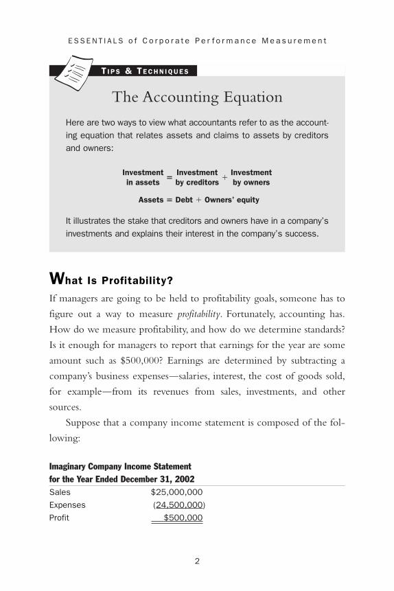
The Accounting Equation
Here are two ways to view what accountants refer to as the account-ing equation that relates assets and claims to assets by creditorsand owners:
It illustrates the stake that creditors and owners have in a company’sinvestments and explains their interest in the company’s success.
Assets � Debt � Owners’ equity
Investmentin assets
�Investmentby creditors
�Investmentby owners
T I P S & TE C H N I Q U E S
What Is Profitability?
If managers are going to be held to profitability goals, someone has to
figure out a way to measure profitability. Fortunately, accounting has.
How do we measure profitability, and how do we determine standards?
Is it enough for managers to report that earnings for the year are some
amount such as $500,000? Earnings are determined by subtracting a
company’s business expenses—salaries, interest, the cost of goods sold,
for example—from its revenues from sales, investments, and other
sources.
Suppose that a company income statement is composed of the fol-
lowing:
Imaginary Company Income Statementfor the Year Ended December 31, 2002Sales $25,000,000
Expenses (24,500,000)
Profit $500,000

3
T h e I m p o r t a n c e o f R e t u r n o n I n v e s t m e n t
Our company has made half a million dollars! Does this mean that
company managers have performed well? Probably not, because for sales
activity of $25,000,000, owners, creditors, and top management would
expect a higher profit: $500,000 is only 2 percent of $25,000,000.
Business people expect that profit must be linked to activity if we are
going to properly measure the adequacy of a company’s profit or judge
the efforts of a company’s management.
Suppose Imaginary Company instead had the following income
statement:
Imaginary Company Income Statement for the Year Ended December 31, 2002Sales $3,125,000
Expenses (2,625,000)
Profit $500,000
It looks like the same half a million, but as we look at the relationship
between profit and activity, where $500,000 in profits is generated by
sales of $3,125,00, we can see that in this scenario the profits are 16 per-
cent of sales.
Still, if we are going to draw conclusions about the profitability, we
need to know more than the absolute dollar amount of profit ($500,000)
and the relationship between profit and activity (16 percent in our exam-
ple).We need to know something about how much money we are earn-
ing relative to our investment.
What Is Return on Investment?
Let’s suppose that the management team for the company represented
by our second income statement, with sales of $3,125,000 and profits of
$500,000, runs a company with assets—plant, equipment, inventories,

4
E S S E N T I A L S o f C o r p o r a t e P e r f o r m a n c e M e a s u r e m e n t
and other items—worth $20,000,000. Does this new information
change our opinion of the performance of the management team? Of
course it does: $500,000 is only 2.5 percent of $20,000,000.A 2.5 per-
cent return on an investment of $20,000,000 is not acceptable! Owners
would be better off with their funds invested in treasury bills (T-bills) or
even in a savings account—the return would be better, and there would
be no risk.A company must generate a much higher return than T-bills
or savings accounts to justify the risk involved in doing business.As our
example shows, return on investment, or ROI, is calculated as follows:
Let’s suppose, instead, that the $500,000 profit was earned using
only $2,000,000 in assets, rather than $20,000,000. ROI is now 25 per-
cent.This return is much higher than the ROI one expects from T-bills,
government bonds, or a bank savings account, and is thus much more
acceptable to owners and creditors.
The relationship between profit and the investment that generates
the profit is one of the most widely used measures of company perfor-
mance. As a quantitative measure of investment and results, ROI pro-
vides a company’s management (as well as the owners and creditors)
ROI �$500,000
$2,000,000� 0.25, or 25.0 percent
ROI �profit
investment
ROI �$500,000
$20,000,000� 0.025, or 2.5 percent
ROI �profit
investment

5
T h e I m p o r t a n c e o f R e t u r n o n I n v e s t m e n t
with a simple tool for examining performance.ROI allows management
to cut out the guesswork and replace it with mathematical calculation,
which can then be used to compare alternative uses of invested capital.
(Should we increase inventory? Or pay off debt?)
Creditors and owners can always invest in government securities that
yield a low rate of return but are essentially risk-free. Riskier investments
require higher rates of return (reward) to attract potential investors. ROI
relates profits (the rewards) to the size of the investment used to gener-
ate it.
How Can ROI Be Useful?
Profits happen when a company operates effectively.We can tell that the
management team is doing its job well if the company prospers, obtains
funding, and rewards the suppliers of its funds. ROI is the principal tool
used to evaluate how well (or poorly) management performs.
Creditors and Owners
ROI is used by creditors and owners to do the following:
1. Assess the company’s ability to earn an adequate rate of return.Creditors and owners can compare the ROI of a company toother companies and to industry benchmarks or norms. ROIprovides information about a company’s financial health.
2. Provide information about the effectiveness of management. TrackingROI over a period of time assists in determining whether a com-pany has capable management.
3. Project future earnings. Potential suppliers of capital assess presentand future investment and the return expected from that invest-ment.
6
E S S E N T I A L S o f C o r p o r a t e P e r f o r m a n c e M e a s u r e m e n t
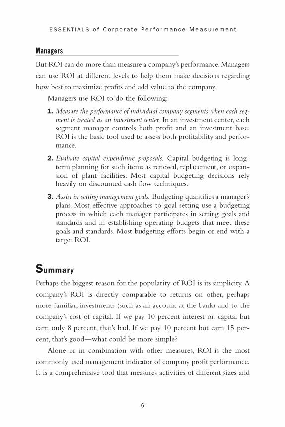
Managers
But ROI can do more than measure a company’s performance.Managers
can use ROI at different levels to help them make decisions regarding
how best to maximize profits and add value to the company.
Managers use ROI to do the following:
1. Measure the performance of individual company segments when each seg-ment is treated as an investment center. In an investment center, eachsegment manager controls both profit and an investment base.ROI is the basic tool used to assess both profitability and perfor-mance.
2. Evaluate capital expenditure proposals. Capital budgeting is long-term planning for such items as renewal, replacement, or expan-sion of plant facilities. Most capital budgeting decisions relyheavily on discounted cash flow techniques.
3. Assist in setting management goals. Budgeting quantifies a manager’splans. Most effective approaches to goal setting use a budgetingprocess in which each manager participates in setting goals andstandards and in establishing operating budgets that meet thesegoals and standards. Most budgeting efforts begin or end with atarget ROI.
Summary
Perhaps the biggest reason for the popularity of ROI is its simplicity. A
company’s ROI is directly comparable to returns on other, perhaps
more familiar, investments (such as an account at the bank) and to the
company’s cost of capital. If we pay 10 percent interest on capital but
earn only 8 percent, that’s bad. If we pay 10 percent but earn 15 per-
cent, that’s good—what could be more simple?
Alone or in combination with other measures, ROI is the most
commonly used management indicator of company profit performance.
It is a comprehensive tool that measures activities of different sizes and
7
T h e I m p o r t a n c e o f R e t u r n o n I n v e s t m e n t
natures and allows us to compare them in a standard way. In other
words, through ROI we can compare apples and oranges, at least in the
area of profitability. ROI has its faults and its advantages. It is sometimes
tricky to use if you do not understand it completely.
That’s what we are going to do in this book—learn to understand
ROI.
Profit Goals May Increase as They Are Delegated
All managers are expected to meet profitability goals, which areoften increased and tightened as each level of management seeksa margin of safety.
Board chair “Let’s target 5 percent profit.”
President “We need 10 percent profit this year.”
Vice president “Your goal is 15 percent.”
Middle manager “We’ve got to turn a 20 percent profit!”
Line manager “Earn 25 percent or else!”
I N T H E RE A L WO R L D

After read ing th is chapter, you wi l l be ab le to
• Understand the relationship between profit margin and assetturnover
• Understand the role of profit margin and asset turnover inprofit planning
• Understand the relationship between return on equity andreturn on investment
• Understand how leverage affects the return on equity
• Understand the advantages and disadvantages of ROI
• Understand the impact on segments of using target ROIs
This ROI thing sounds sort of interesting, but who uses it? Many
senior managers use ROI because it is an overall measure that is
affected by a manager’s activity in many different areas. Let’s con-
sider, for example, two hypothetical managers of companies that have
each earned a profit of $20,000 on an investment of $100,000, to pro-
duce ROIs of 20 percent.
Jones Company: ROI �$20,000
$100,000� 20%
Smith Company: ROI �$20,000$100,000
� 20%
CHAPTER 2
9
Using ROI to AnalyzePerformance

1 0
E S S E N T I A L S o f C o r p o r a t e P e r f o r m a n c e M e a s u r e m e n t
Our two managers produced the same ROI, but are their business
activities otherwise the same? Is it possible that they arrived at the same
ROI by completely different strategies?
Relationship between Profit Margin and AssetTurnover
Let’s imagine that both companies are retail jewelers. Smith Company
sells inexpensive costume jewelry in malls throughout the country.
Smith Company follows a high-volume, low-markup approach to mar-
keting.Thus, the profit margin on Smith Company sales is only 4 per-
cent, calculated as follows:
Smith Company turns its assets over rapidly.Although asset turnover
is a somewhat intuitive concept, analysts calculate it by dividing an asset
into the best measure of the asset’s activity. Sales is the best measure of
the activity of total assets. If Smith Company creates sales of $500,000
with its investment of $100,000, its asset turnover is 5 times per year,
calculated as follows:
We can see that the ROI generated by Smith Company (20 percent)
is the product of Smith Company’s investment turnover (5 times) and
its profit margin on sales (.04).The investment turnover is a measure of
how active Smith Company has been. The profit margin on sales is a
measure of how profitable that activity has been. Because Smith
Company is very active, the profit margin on each sale can be low.
Smith Companyinvestment
turnover�
salesinvestment
�$500,000$100,000
� 5 times
Profit margin on sales �profitsales
�$20,000$500,000
� .04
1 1
U s i n g R O I t o A n a l y z e P e r f o r m a n c e
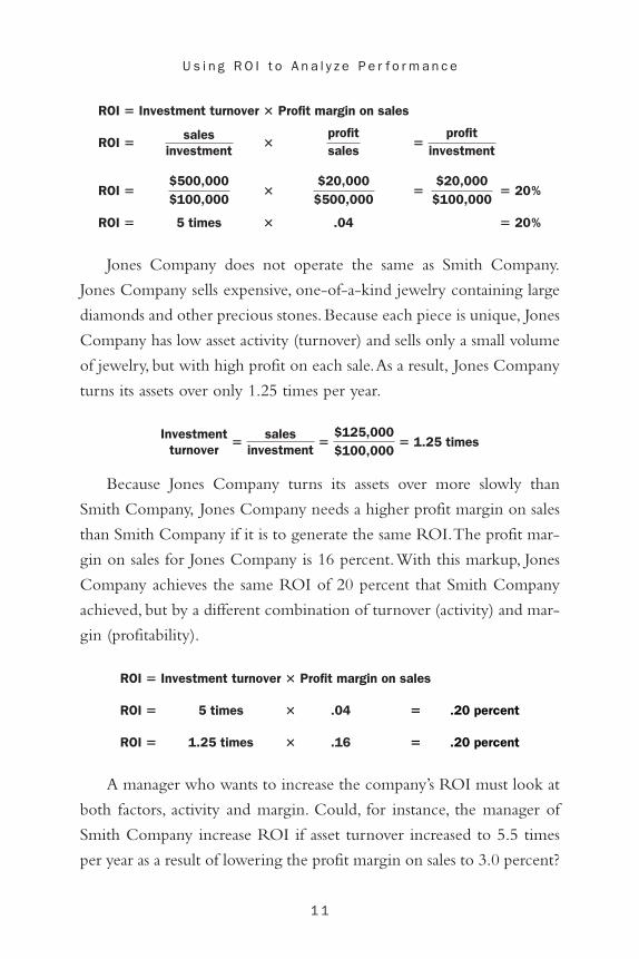
Jones Company does not operate the same as Smith Company.
Jones Company sells expensive, one-of-a-kind jewelry containing large
diamonds and other precious stones. Because each piece is unique, Jones
Company has low asset activity (turnover) and sells only a small volume
of jewelry, but with high profit on each sale.As a result, Jones Company
turns its assets over only 1.25 times per year.
Because Jones Company turns its assets over more slowly than
Smith Company, Jones Company needs a higher profit margin on sales
than Smith Company if it is to generate the same ROI.The profit mar-
gin on sales for Jones Company is 16 percent.With this markup, Jones
Company achieves the same ROI of 20 percent that Smith Company
achieved, but by a different combination of turnover (activity) and mar-
gin (profitability).
A manager who wants to increase the company’s ROI must look at
both factors, activity and margin. Could, for instance, the manager of
Smith Company increase ROI if asset turnover increased to 5.5 times
per year as a result of lowering the profit margin on sales to 3.0 percent?
ROI �
ROI �
ROI �
Investment turnover
5 times
1.25 times
�
�
�
Profit margin
.04
.16
on sales �
�
�
.
.20 percent
.20 percent
Investmentturnover
�sales
investment�
$125,000$100,000
� 1.25 times
20%
20%
�
�
profitinvestment
$20,000$100,000
�
�
Profit margin on sales
profitsales
$20,000$500,000
.04
�
�
�
�
Investment turnover
salesinvestment
$500,000$100,000
5 times
ROI �
ROI �
ROI �
ROI �

1 2
E S S E N T I A L S o f C o r p o r a t e P e r f o r m a n c e M e a s u r e m e n t
5.5 times � .03 � .165
No, that will not work. ROI would decrease to 16.5 percent. But
the manager can calculate the profit margin necessary to increase ROI
to a targeted 22 percent with a turnover of 5.5 times per year.
The manager must turn assets 5.5 times with a .04 profit margin on
sales in order to generate a 22 percent ROI.
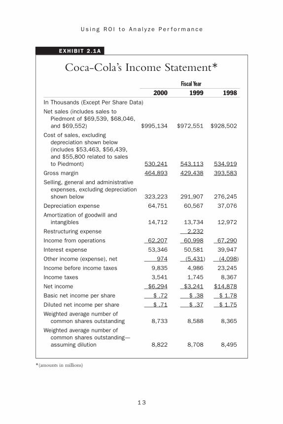
Coca-Cola and Ford
Even though two companies might be in different industries, they can
still demonstrate the phenomena just discussed. Coca-Cola Bottling and
Ford (the automotive division) had nearly the same ROIs in 2000.The
income statements and balance sheets of these two companies are in
Exhibits 2.1a—b and 2.2a—b.Their ROIs are calculated using net oper-
ating income as the return. Operating income is a company’s income from
its regular business operations. Operating income is thought to be a bet-
ter measure of the earnings that a company can continue year after year,
than is net income, which is affected by unusual gains and losses or
changes in debt and interest expense.
As we have already seen, companies can generate similar ROIs in
quite different ways. So how did Coca-Cola and Ford create these
returns? What strategies did their managers take? Let’s separate the ROIs
Ford Motor ROI �
profit 1net 21operating system 2
investment�
$5,226$95,343
� .0548
Coca-Cola ROI �
profit 1net 21operating system 2investment
�$62,207
$1,062,097� .0586
Margin �.22 target ROI
5.5 times� .04
5.5 times � profit � .22 target ROI
1 3
U s i n g R O I t o A n a l y z e P e r f o r m a n c e
EXHIBIT 2 .1A
Coca-Cola’s Income Statement*Fiscal Year
2000 1999 1998In Thousands (Except Per Share Data)
Net sales (includes sales to Piedmont of $69,539, $68,046, and $69,552) $995,134 $972,551 $928,502
Cost of sales, excluding depreciation shown below (includes $53,463, $56,439, and $55,800 related to sales to Piedmont) 530,241 543,113 534,919
Gross margin 464,893 429,438 393,583
Selling, general and administrative expenses, excluding depreciation shown below 323,223 291,907 276,245
Depreciation expense 64,751 60,567 37,076
Amortization of goodwill and intangibles 14,712 13,734 12,972
Restructuring expense 2,232
Income from operations 62,207 60,998 67,290
Interest expense 53,346 50,581 39,947
Other income (expense), net 974 (5,431) (4,098)
Income before income taxes 9,835 4,986 23,245
Income taxes 3,541 1,745 8,367
Net income $6,294 $3,241 $14,878
Basic net income per share $ .72 $ .38 $ 1.78
Diluted net income per share $ .71 $ .37 $ 1.75
Weighted average number of common shares outstanding 8,733 8,588 8,365
Weighted average number of common shares outstanding—assuming dilution 8,822 8,708 8,495
*(amounts in millions)

1 4
E S S E N T I A L S o f C o r p o r a t e P e r f o r m a n c e M e a s u r e m e n t
EXHIBIT 2 .1B
Coca-Cola Balance Sheet
In Thousands (Except Share Data)ASSETS
Current assets:CashAccounts receivable, trade, less allowance for doubtful accounts
of $918 and $850Accounts receivable from The Coca-Cola CompanyAccounts receivable, otherInventories
Prepaid expenses and other current assetsTotal current assets
Property, plant and equipment, netLeased property under capital leases, netInvestment in Piedmont Coca-Cola Bottling PartnershipOther assetsIdentifiable intangible assets, netExcess of cost over fair value of net assets of businesses
acquired, less accumulated amortization of $35,585 and $33,141Total
LIABILITIES AND STOCKHOLDERS’ EQUITYCurrent liabilities:Portion of long-term debt payable within one yearCurrent portion of obligations under capital leasesAccounts payable and accrued liabilitiesAccounts payable to The Coca-Cola CompanyDue to Piedmont Coca-Cola Bottling PartnershipAccrued interest payable
Total current liabilities
Deferred income taxes
Other liabilitiesObligations under capital leases

1 5
U s i n g R O I t o A n a l y z e P e r f o r m a n c e
Dec. 31, 2000 Jan. 2, 2000
$8,425 $9,05062,661 60,367
5,380 6,0188,247 13,938
40,502 41,411
14,026 13,275139,241 144,059429,978 468,110
7,948 10,78562,730 60,21660,846 61,312
284,842 305,783
76,512 58,127$1,062,097 $1,108,392
$ 9,904 $ 28,6353,325 4,483
80,999 96,0083,802 2,346
16,436 2,73610,483 16,830
124,949 151,038
148,655 124,171
76,061 73,9001,774 4,468
continues

1 6
E S S E N T I A L S o f C o r p o r a t e P e r f o r m a n c e M e a s u r e m e n t
EXHIBIT 2 .1B
CO C A -CO L A’S BA L A N C E SH E E T C O N T I N U E D
Long-term debtTotal liabilities
Commitments and Contingencies (Note 11)
Stockholders’ Equity:Convertible Preferred Stock, $100 par value: Authorized—
50,000 shares; Issued—NoneNonconvertible Preferred Stock, $100 par value: Authorized—
50,000 shares; Issued—NonePreferred Stock, $.01 par value: Authorized—20,000,000
shares; Issued—NoneCommon Stock, $1 par value: Authorized—30,000,000 shares;
Issued—9,454,651 and 9,454,626 sharesClass B Common Stock, $1 par value: Authorized—
10,000,000 shares; Issued 2,969,166 and 2,969,191 shares
Class C Common Stock, $1 par value: Authorized—20,000,000 shares; Issued—None
Capital in excess of par valueAccumulated deficit
Less—Treasury stock, at cost:Common—3,062,374 sharesClass B Common—628,114 sharesTotal stockholders’ equity
Total
into their investment turnover and profit margin components. Ford has
an asset turnover of more than 1.5 times that of Coca-Cola, while
Coca-Cola has a profit margin on sales 1.7 times that of Ford. Ford fol-
lowed a strategy of more active asset use; Coca-Cola had more profitable
sales. (The details of these calculations are in Exhibit 2.3.)

1 7
U s i n g R O I t o A n a l y z e P e r f o r m a n c e
Dec. 31, 2000 Jan. 2, 2000682,246 723,964
1,033,685 1,077,541
9,454 9,454
2,969 2,969
99,020 107,753(21,777) (28,071)89,666 92,105
60,845 60,845 409 409
28,412 30,851$1,062,097 $1,108,392
ROI
Coca-Cola ROI
Ford Motor ROI
�
�
�
Investment turnover
.937 times
1.4813 times
�
�
�
Profit margin
.063
.037
�
�
�
.058
.055
1 8
E S S E N T I A L S o f C o r p o r a t e P e r f o r m a n c e M e a s u r e m e n t
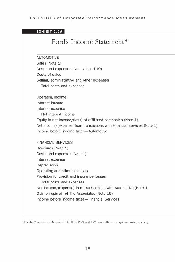
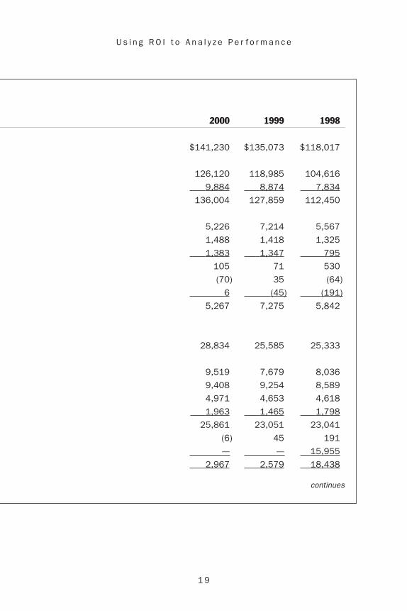
EXHIBIT 2 .2A
Ford’s Income Statement*
AUTOMOTIVE
Sales (Note 1)
Costs and expenses (Notes 1 and 19)
Costs of sales
Selling, administrative and other expenses
Total costs and expenses
Operating income
Interest income
Interest expense
Net interest income
Equity in net income/(loss) of affiliated companies (Note 1)
Net income/(expense) from transactions with Financial Services (Note 1)
Income before income taxes—Automotive
FINANCIAL SERVICES
Revenues (Note 1)
Costs and expenses (Note 1)
Interest expense
Depreciation
Operating and other expenses
Provision for credit and insurance losses
Total costs and expenses
Net income/(expense) from transactions with Automotive (Note 1)
Gain on spin-off of The Associates (Note 19)
Income before income taxes—Financial Services
*For the Years Ended December 31, 2000, 1999, and 1998 (in millions, except amounts per share)
1 9
U s i n g R O I t o A n a l y z e P e r f o r m a n c e
2000 1999 1998
$141,230 $135,073 $118,017
126,120 118,985 104,616
9,884 8,874 7,834
136,004 127,859 112,450
5,226 7,214 5,567
1,488 1,418 1,325
1,383 1,347 795
105 71 530
(70) 35 (64)
6 (45) (191)
5,267 7,275 5,842
28,834 25,585 25,333
9,519 7,679 8,036
9,408 9,254 8,589
4,971 4,653 4,618
1,963 1,465 1,798
25,861 23,051 23,041
(6) 45 191
— — 15,955
2,967 2,579 18,438
continues
2 0
E S S E N T I A L S o f C o r p o r a t e P e r f o r m a n c e M e a s u r e m e n t
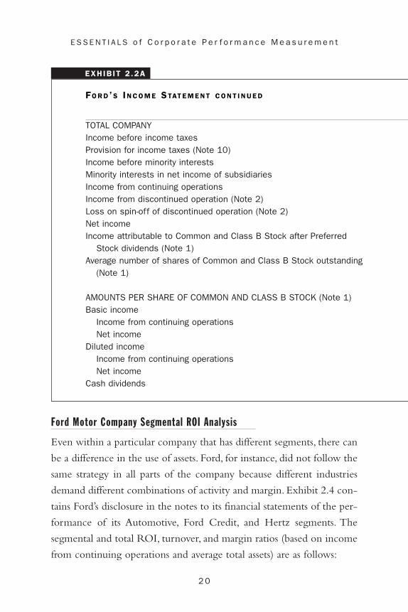
EXHIBIT 2 .2A
FO R D’S IN C O M E STAT E M E N T C O N T I N U E D
TOTAL COMPANYIncome before income taxesProvision for income taxes (Note 10)Income before minority interestsMinority interests in net income of subsidiariesIncome from continuing operationsIncome from discontinued operation (Note 2)Loss on spin-off of discontinued operation (Note 2)Net incomeIncome attributable to Common and Class B Stock after Preferred
Stock dividends (Note 1)Average number of shares of Common and Class B Stock outstanding
(Note 1)
AMOUNTS PER SHARE OF COMMON AND CLASS B STOCK (Note 1)Basic income
Income from continuing operationsNet income
Diluted incomeIncome from continuing operationsNet income
Cash dividends
Ford Motor Company Segmental ROI Analysis
Even within a particular company that has different segments, there can
be a difference in the use of assets. Ford, for instance, did not follow the
same strategy in all parts of the company because different industries
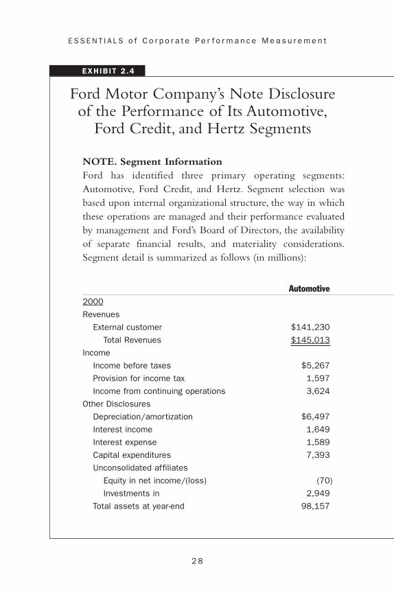
demand different combinations of activity and margin. Exhibit 2.4 con-
tains Ford’s disclosure in the notes to its financial statements of the per-
formance of its Automotive, Ford Credit, and Hertz segments. The
segmental and total ROI, turnover, and margin ratios (based on income
from continuing operations and average total assets) are as follows:

2 1
U s i n g R O I t o A n a l y z e P e r f o r m a n c e
2000 1999 1998
8,234 9,854 24,2802,705 3,248 2,7605,529 6,606 21,520
119 104 1525,410 6,502 21,368
309 735 703(2,252) — —$3,467 $7,237 $22,071
$3,452 $7,222 $21,964
1,483 1,210 1,211
$3.66 $5.38 $17.592.34 5.99 18.17
$3.59 $ 5.26 $17.192.30 5.86 17.76
$1.80 $1.88 $1.72
Ford’s Automotive and Hertz segments have a greater ROI than
the company as a whole; the Ford Credit segment’s ROI is lower.The
�
�
�
�
�
Investment turnover
1.445
.143
.490
.613
�
�
�
�
�
Profit margin
.025
.065
.070
.032
�
�
�
�
�
1
.036
.009
.034
.020
ROI
Automotive ROI
Ford Credit ROI
Hertz ROI
Total ROI 1from three segments 2
2 2
E S S E N T I A L S o f C o r p o r a t e P e r f o r m a n c e M e a s u r e m e n t
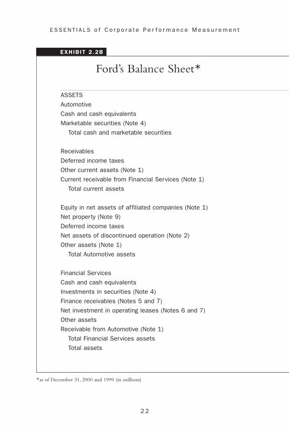
EXHIBIT 2 .2B
Ford’s Balance Sheet*
ASSETS
Automotive
Cash and cash equivalents
Marketable securities (Note 4)
Total cash and marketable securities
Receivables
Deferred income taxes
Other current assets (Note 1)
Current receivable from Financial Services (Note 1)
Total current assets
Equity in net assets of affiliated companies (Note 1)
Net property (Note 9)
Deferred income taxes
Net assets of discontinued operation (Note 2)
Other assets (Note 1)
Total Automotive assets
Financial Services
Cash and cash equivalents
Investments in securities (Note 4)
Finance receivables (Notes 5 and 7)
Net investment in operating leases (Notes 6 and 7)
Other assets
Receivable from Automotive (Note 1)
Total Financial Services assets
Total assets
*as of December 31, 2000 and 1999 (in millions)

2 3
U s i n g R O I t o A n a l y z e P e r f o r m a n c e
2000 1999
$3,374 $2,793
13,116 18,943
16,490 21,736
4,685 5,267
2,239 3,762
5,318 3,831
1,587 2,304
37,833 42,584
2,949 2,539
37,508 36,528
3,342 2,454
— 1,566
13,711 13,530
95,343 99,201
1,477 1,588
817 733
125,164 113,298
46,593 42,471
12,390 11,123
2,637 1,835
189,078 171,048
$284,421 $270,249
continues

2 4
E S S E N T I A L S o f C o r p o r a t e P e r f o r m a n c e M e a s u r e m e n t
EXHIBIT 2 .2B
FO R D’S BA L A N C E STAT E M E N T C O N T I N U E D
LIABILITIES AND STOCKHOLDERS’ EQUITYAutomotiveTrade payablesOther payablesAccrued liabilities (Note 11)Income taxes payableDebt payable within one year (Note 13)
Total current liabilities
Long-term debt (Note 13)Other liabilities (Note 11)Deferred income taxesPayable to Financial Services (Note 1)
Total Automotive liabilities
Financial ServicesPayablesDebt (Note 13)Deferred income taxesOther liabilities and deferred incomePayable to Automotive (Note 1)
Total Financial Services liabilities
Company-obligated mandatorily redeemable preferred securities of a subsidiary trust holding solely junior subordinated debentures of the Company (Note 1)
Stockholders’ equityCapital stock (Notes 14 and 15)
Preferred Stock, par value $1.00 per share (aggregate liquidation preference of $177 million)Common Stock (par value $0.01 and $1.00 per share as of 2000 and 1999, respectively; 1.837 and 1.151 million shares issued
as of 2000 and 1999, respectively) (Note 3)

2 5
U s i n g R O I t o A n a l y z e P e r f o r m a n c e
2000 1999
$ 15,075 $ 14,2924,011 3,778
23,515 18,488449 1,709
277 1,33843,327 39,605
11,769 10,39830,495 29,283
353 1,2232,637 1,835
88,581 82,344
5,297 3,550153,510 139,919
8,677 7,0787,486 6,7751,587 2,304
176,557 159,626
673 675
* *
18 1,151
continues
2 6
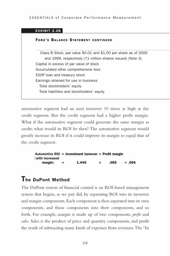
E S S E N T I A L S o f C o r p o r a t e P e r f o r m a n c e M e a s u r e m e n t
EXHIBIT 2 .2B
FO R D’S BA L A N C E STAT E M E N T C O N T I N U E D
Class B Stock, par value $0.01 and $1.00 per share as of 2000
and 1999, respectively (71 million shares issued) (Note 3)
Capital in excess of par value of stock
Accumulated other comprehensive loss
ESOP loan and treasury stock
Earnings retained for use in business
Total stockholders’ equity
Total liabilities and stockholders’ equity
automotive segment had an asset turnover 10 times as high as the
credit segment. But the credit segment had a higher profit margin.
What if the automotive segment could generate the same margin as
credit; what would its ROI be then? The automotive segment would
greatly increase its ROI if it could improve its margin to equal that of
the credit segment.
The DuPont Method
The DuPont system of financial control is an ROI-based management
system that begins, as we just did, by separating ROI into its turnover
and margin components. Each component is then separated into its own
components, and those components into their components, and so
forth. For example, margin is made up of two components, profit and
sales. Sales is the product of price and quantity components, and profit
the result of subtracting many kinds of expenses from revenues.The “In
Automotive ROI1with increased 21margin 2�
�
Investment turnover
1.445
�
�
Profit margin
.065 � .094

2 7
U s i n g R O I t o A n a l y z e P e r f o r m a n c e
2000 1999
1 71
6,174 5,049
(3,432) (1,856)
(2,035) (1,417)
17,884 24,606
18,610 27,604
$284,421 $270,249
EXHIBIT 2 .3
Ratio Calculations for Coca-Cola and Ford
.0548
.0548
�
�
Profit Margin
profitsales
$5,226$141,230
.0370
�
�
�
Investment Turnover
salesinvestment
$141,230$95,343
1.4813 times
Ford Motor ROI �
�
�
.0586
.0586
�
�
Profit margin
profitsales
$62,207$995,134
.0625
�
�
�
�
Investment turnover
salesinvestment
$995,134$1,062,097
.9370 times
ROI �
Coca-Cola ROI �
�
�
2 8
E S S E N T I A L S o f C o r p o r a t e P e r f o r m a n c e M e a s u r e m e n t
EXHIBIT 2 .4
Ford Motor Company’s Note Disclosure of the Performance of Its Automotive,
Ford Credit, and Hertz Segments
NOTE. Segment InformationFord has identified three primary operating segments:Automotive, Ford Credit, and Hertz. Segment selection wasbased upon internal organizational structure, the way in whichthese operations are managed and their performance evaluatedby management and Ford’s Board of Directors, the availabilityof separate financial results, and materiality considerations.Segment detail is summarized as follows (in millions):
Automotive2000
Revenues
External customer $141,230
Total Revenues $145,013
Income
Income before taxes $5,267
Provision for income tax 1,597
Income from continuing operations 3,624
Other Disclosures
Depreciation/amortization $6,497
Interest income 1,649
Interest expense 1,589
Capital expenditures 7,393
Unconsolidated affiliates
Equity in net income/(loss) (70)
Investments in 2,949
Total assets at year-end 98,157

2 9
U s i n g R O I t o A n a l y z e P e r f o r m a n c e
Financial Services Sector
Ford Credit Hertz Other Fin Svcs Elims/Other Total
$ 23,412 $5,057 342 23 $170,064
$ 23,606 $5,087 $496 $(4,138) $170,064
$2,495 $581 $(109) $— $8,234
926 223 (41) — 2,705
1,536 358 (35) (73) 5,410
$7,846 a/ $ 1,504 $46 $56 $ 15,949
— — — (161) 1,488
8,970 428 459 (544) 10,902
168 291 496 — 8,348
(22) — 1 — (91)
79 — 7 — 3,035
174,258 10,620 7,668 (6,282) 284,421
continues
3 0
E S S E N T I A L S o f C o r p o r a t e P e r f o r m a n c e M e a s u r e m e n t
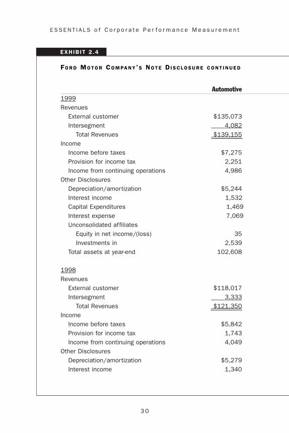
EXHIBIT 2 .4
FO R D MO T O R CO M PA N Y ’S NO T E D I S C L O S U R E C O N T I N U E D
Automotive1999Revenues
External customer $135,073Intersegment 4,082
Total Revenues $139,155Income
Income before taxes $7,275Provision for income tax 2,251Income from continuing operations 4,986
Other DisclosuresDepreciation/amortization $5,244Interest income 1,532Capital Expenditures 1,469Interest expense 7,069Unconsolidated affiliates
Equity in net income/(loss) 35Investments in 2,539
Total assets at year-end 102,608
1998Revenues
External customer $118,017Intersegment 3,333
Total Revenues $121,350Income
Income before taxes $5,842Provision for income tax 1,743Income from continuing operations 4,049
Other DisclosuresDepreciation/amortization $5,279Interest income 1,340

3 1
U s i n g R O I t o A n a l y z e P e r f o r m a n c e
Financial Services Sector
Ford Credit Hertz Other Fin Svcs Elims/Other Total
$20,020 $4,695 $866 $4 $160,658340 33 170 (4,625) —
$20,360 $4,728 $1,036 $(4,621) $160,658
$2,104 $560 $(85) $ — $9,854791 224 (18) — 3,248
1,261 336 (15) (66) 6,502
$7,565 a/ $1,357 $326 $50 $14,542— — — (114) 1,418
7,193 354 633 (623) 9,02682 351 157 — 7,659
(25) — — — 1097 — 8 — 2,644
156,631 10,137 12,427 (11,554) 270,249
$19,095 $4,241 $1,997 $ — $143,350208 9 272 (3,822) —
$19,303 $4,250 $2,269 $(3,822) $143,350
$1,812 $465 $16,161 b/ $ — $24,280680 188 149 — 2,760
1,084 277 16,060 b/ (102) 21,368
$7,327 a/ $ 1,212 $54 $31 $13,903— — — (15) 1,325
continues
3 2
E S S E N T I A L S o f C o r p o r a t e P e r f o r m a n c e M e a s u r e m e n t
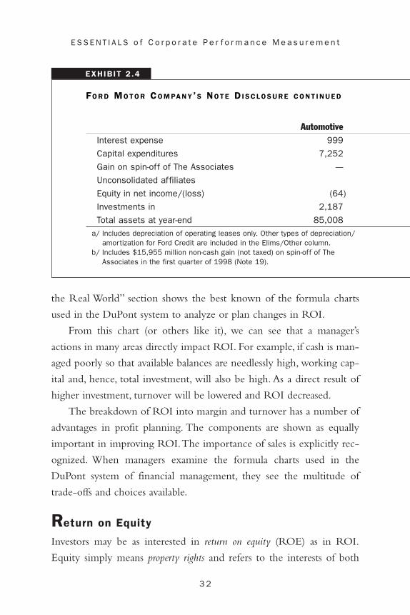
EXHIBIT 2 .4
FO R D MO T O R CO M PA N Y ’S NO T E D I S C L O S U R E C O N T I N U E D
AutomotiveInterest expense 999
Capital expenditures 7,252
Gain on spin-off of The Associates — —
Unconsolidated affiliates
Equity in net income/(loss) (64)
Investments in 2,187
Total assets at year-end 85,008a/ Includes depreciation of operating leases only. Other types of depreciation/
amortization for Ford Credit are included in the Elims/Other column.b/ Includes $15,955 million non-cash gain (not taxed) on spin-off of The
Associates in the first quarter of 1998 (Note 19).
the Real World” section shows the best known of the formula charts
used in the DuPont system to analyze or plan changes in ROI.
From this chart (or others like it), we can see that a manager’s
actions in many areas directly impact ROI. For example, if cash is man-
aged poorly so that available balances are needlessly high, working cap-
ital and, hence, total investment, will also be high. As a direct result of
higher investment, turnover will be lowered and ROI decreased.
The breakdown of ROI into margin and turnover has a number of
advantages in profit planning. The components are shown as equally
important in improving ROI.The importance of sales is explicitly rec-
ognized. When managers examine the formula charts used in the
DuPont system of financial management, they see the multitude of
trade-offs and choices available.
Return on Equity
Investors may be as interested in return on equity (ROE) as in ROI.
Equity simply means property rights and refers to the interests of both

3 3
U s i n g R O I t o A n a l y z e P e r f o r m a n c e
Financial Services Sector
Ford Credit Hertz Other Fin Svcs Elims/Other Total6,910 318 1,114 (510) 8,831
67 317 120 — 7,756
— — 15,955 — 15,955
2 — — — (62)
76 — — — 2,263
137,248 8,873 6,181 (4,598) 232,712
owners and creditors, but the equity in ROE is defined as shareholder
equity only.Thus, ROE measures the return on shareholders’ investment
in the company rather than the return on the company’s investment in
assets. For an investor, this is the most important return.
The Effect of Debt on the ROE
ROE differs from ROI because a company typically borrows part of its
capital. Consider a company that creates a 15 percent ROI, as follows.
If all the investment in assets ($900,000) is financed by owners, then
owners’ equity is also $900,000 and ROE is also 15 percent.
But if one-third of the investment in assets is borrowed, and own-
ers’ equity is only $600,000, ROE is increased to 22.5 percent. If half
ROE �profitequity
�$135,000$900,000
� .15
ROI �profit
investment�
$135,000$900,000
� .15

3 4
E S S E N T I A L S o f C o r p o r a t e P e r f o r m a n c e M e a s u r e m e n t
A Formula Chart Used in the DuPont System of Financial Management
I N T H E RE A L WO R L D
Mill costof sales
Sellingexpense
Administrativeexpense
Plus
Plus
Inventories
Accountsreceivable
Cash
PlusWorkingcapital
Permanentinvestment
Plus
Sales
Cost of sales
MinusEarnings
Earnings as% of sales
Return onInvestment
Sales
Divided by
Multiplied bySales
Turnover
Totalinvestment
Divided by
Plus
the assets are from borrowed capital, ROE rises to 30 percent.At three-
quarters debt, ROE is 45 percent.
The following summary calculations highlight the effect of
increased debt on the ROE.As the relative amount of debt increases, the
ROE also increases.
The proportion of assets obtained by debt financing rather than
owner investment is quite important, because debt leverages the owners’
investment.
ROE �profitequity
�$135,000$600,000
� .225
ROE �profitequity
�$135,000$450,000
� .30
ROE �profitequity
�$135,000$400,000
� .45

3 5
U s i n g R O I t o A n a l y z e P e r f o r m a n c e
A lever placed across a fulcrum transfers pressure on the long end of
the lever into a greatly magnified force on the short end, giving a pow-
erful mechanical advantage. In the same sense, financial leverage gives a
financial advantage, increasing ROE when companies borrow and then
earn an ROI on the borrowed funds greater than the interest rate.
Although the interest lowers earnings somewhat, the owners’ invest-
ment is much smaller and the effect of earnings is magnified, increasing
the return on the owners’ equity (ROE). Although we omit implicit
consideration of interest here, increasing debt generally increases ROE.
The Effect of Debt on Solvency
Ratios of debt and equity are called solvency or leverage ratios. Examples
include debt to owners’ equity, debt to total equities (debt plus owners’
equity), and the inverse of these ratios. Debt and equity ratios determine
the relative sizes of the property rights of creditors and owners. Too
much debt restricts managers and increases the risk of owners because
Financial Leverage as a MagnifierFinancial leverage (FL) or solvency is greater than 1.0 when a com-pany has debt, and therefore acts like a magnifier when multipliedby the ROI to obtain the ROE.
22.5%�.225�
1.5�.15�
$900,000$600,000
�$135,000$900,000
�
assetsequity
�profit
assets�
FL�ROI�ROE
T I P S & TE C H N I Q U E S

3 6
E S S E N T I A L S o f C o r p o r a t e P e r f o r m a n c e M e a s u r e m e n t
debt increases the fixed charges (interest expense) against income each
period. Special-purpose ratios, such as the times interest earned or the
fixed charge coverage ratios show the burden of fixed charges (such as
interest or lease payments) and whether the company generates the
earnings to pay them.
The proportion of income that interest and other fixed charges can
safely consume varies from industry to industry.The ratios are used as
general guidelines, similar to bank guidelines that say a consumer’s
house payment or car payment should be no more than a certain pro-
portion of the consumer’s income.
As the proportion of debt rises, creditors are more and more reluc-
tant to lend. Eventually, credit will be available only at very high inter-
est rates. Still, a certain amount of debt is good for owners because
managers use debt to increase ROE, as we saw earlier.
ROI, ROE, and Solvency
We know margin times turnover equals ROI. By adding a solvency
ratio, we can add information and expand these basic components to
analyze ROE as well as ROI.The solvency ratio we add is total invest-
ment in assets divided by owners’ equity.When we add this component
to ROI, algebraically we get ROE.
Returning to the examples of Coca-Cola and Ford Motor, we can
determine that the ROIs, turnovers, and margins for these companies
are as follows.
11
11solvency1
investmentowners' equity
�
�
profit marginon sales
profit marginon sales
incomesales
�
�
�
investmentturnover
investmentturnover
salesinvestment
11ROI �
11ROE �
11ROE �
3 7
U s i n g R O I t o A n a l y z e P e r f o r m a n c e
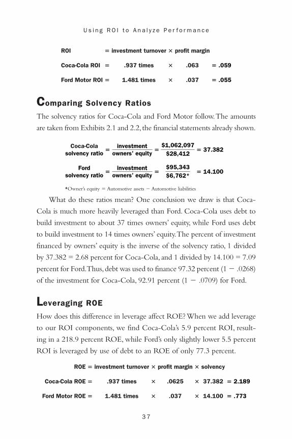
Comparing Solvency Ratios
The solvency ratios for Coca-Cola and Ford Motor follow.The amounts
are taken from Exhibits 2.1 and 2.2, the financial statements already shown.
*Owner’s equity � Automotive assets � Automotive liabilities
What do these ratios mean? One conclusion we draw is that Coca-
Cola is much more heavily leveraged than Ford. Coca-Cola uses debt to
build investment to about 37 times owners’ equity, while Ford uses debt
to build investment to 14 times owners’ equity.The percent of investment
financed by owners’ equity is the inverse of the solvency ratio, 1 divided
by 37.382 = 2.68 percent for Coca-Cola, and 1 divided by 14.100 = 7.09
percent for Ford.Thus,debt was used to finance 97.32 percent (1 � .0268)
of the investment for Coca-Cola, 92.91 percent (1 � .0709) for Ford.
Leveraging ROE
How does this difference in leverage affect ROE? When we add leverage
to our ROI components, we find Coca-Cola’s 5.9 percent ROI, result-
ing in a 218.9 percent ROE, while Ford’s only slightly lower 5.5 percent
ROI is leveraged by use of debt to an ROE of only 77.3 percent.
ROE �
Coca-Cola ROE �
Ford Motor ROE �
investment turnover
.937 times
1.481 times
�
�
�
profit margin
.0625
.037
�
�
�
solvency
37.382
14.100
�
� 2.189
� .773
Coca-Colasolvency ratio
Fordsolvency ratio
�investment
owners' equity�
�investment
owners' equity�
$1,062,097$28,412
$95,343$6,762*
� 37.38211
� 14.10011
ROI
Coca-Cola ROI
Ford Motor ROI
�
�
�
investment turnover
.937 times
1.481 times
�
�
�
profit margin
.063
.037
�
�
�
.059
.055

3 8
E S S E N T I A L S o f C o r p o r a t e P e r f o r m a n c e M e a s u r e m e n t
Notice how Coca-Cola and Ford Motor had similar ROIs, but
their debt levels (shown by the solvency ratio) produced drastically dif-
ferent ROEs.
But, how typical is an ROE of 77 percent or 219 percent? When the
average ROE of the Standard & Poor’s 500 companies reached 20.12
percent in the first quarter of 1995—the highest level since World War
II—the Wall Street Journal said an ROE of 20 percent was equivalent to
a baseball player hitting .350.1 But the Wall Street Journal was speaking
of ROE calculated using net income after tax rather than operating earn-
ings, as we used in our calculations.When we determine ROE using net
income (the final bottom line), activities and events other than opera-
tions cause ROE for Coca-Cola to be 22.2 percent, and for Ford,
18.639 percent.
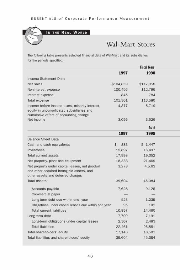
Selected financial data for Wal-Mart are included in this chapter.Using
bottom-line net income,Wal-Mart’s profit margin on sales is 3.3 percent,
its investment turnover is 2.45, and its ratio of investment to owners’ equity
is 2.49.Wal-Mart’s 2000 ROI is 8.06 percent and its ROE is 20.08 percent.
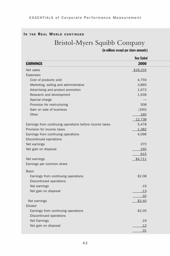
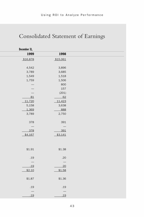
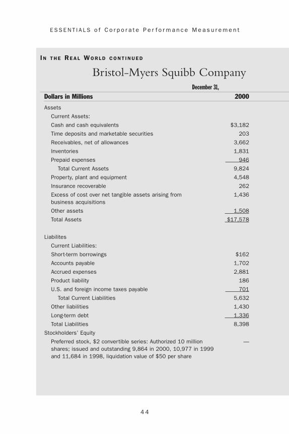
But some companies do even better. The 2000 balance sheet and
income statement for Bristol-Myers Squibb are also included in this chap-
ter.Again using net income rather than operating earnings, Bristol-Myers
has a profit margin on sales of 25.86 percent, an investment turnover of
1.04, and a ratio of investment to owners’ equity of 1.91. Bristol-Myers’
ROI is 26.8 percent and its ROE is an astounding 51.4 percent.
Notice the different approaches managers use to achieve profitabil-
ity in these companies in two completely different business environ-
ments: the debt levels of the two companies are not that different, but
ROE �
Wal-Mart ROE �
Bristol-Myers ROE �
investment turnover
2.45
1.04
�
�
�
profit margin
.033
.259
�
�
�
solvency
2.49
1.91
�
� .201
� .514
3 9
U s i n g R O I t o A n a l y z e P e r f o r m a n c e
Bristol-Myers has a very high profit margin, while Wal-Mart has a very
low profit margin. Wal-Mart, however, turns over total assets (invest-
ments) about 2.5 times while Bristol-Myers turns assets (investments)
only one time. Each company’s strategy is appropriate to its business
environment and successful in its own way.
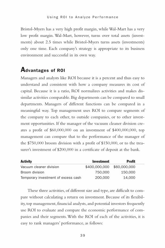
Advantages of ROI
Managers and analysts like ROI because it is a percent and thus easy to
understand and consistent with how a company measures its cost of
capital. Because it is a ratio, ROI normalizes activities and makes dis-
similar activities comparable. Big departments can be compared to small
departments. Managers of different functions can be compared in a
meaningful way. Top management uses ROI to compare segments of
the company to each other, to outside companies, or to other invest-
ment opportunities. If the manager of the vacuum cleaner division cre-
ates a profit of $60,000,000 on an investment of $400,000,000, top
management can compare that to the performance of the manager of
the $750,000 broom division with a profit of $150,000, or to the trea-
surer’s investment of $200,000 in a certificate of deposit at the bank.
Activity Investment Profit Vacuum cleaner division $400,000,000 $60,000,000
Broom division 750,000 150,000
Temporary investment of excess cash 200,000 14,000
These three activities, of different size and type, are difficult to com-
pare without calculating a return on investment. Because of its flexibil-
ity, top management, financial analysts, and potential investors frequently
use ROI to evaluate and compare the economic performance of com-
panies and their segments.With the ROI of each of the activities, it is
easy to rank managers’ performance, as follows:
4 0
E S S E N T I A L S o f C o r p o r a t e P e r f o r m a n c e M e a s u r e m e n t
Wal-Mart StoresThe following table presents selected financial data of Wal-Mart and its subsidiaries
for the periods specified.
Fiscal Years
1997 1998Income Statement Data
Net sales $104,859 $117,958
Noninterest expense 100,456 112,796
Interest expense 845 784
Total expense 101,301 113,580
Income before income taxes, minority interest, 4,877 5,719equity in unconsolidated subsidiaries and cumulative effect of accounting changeNet income 3,056 3,526
As of
1997 1998Balance Sheet Data
Cash and cash equivalents $ 883 $ 1,447
Inventories 15,897 16,497
Total current assets 17,993 19,352
Net property, plant and equipment 18,333 21,469
Net property under capital leases, net goodwill 3,278 4,5.63and other acquired intangible assets, and other assets and deferred charges
Total assets 39,604 45,384
Accounts payable 7,628 9,126
Commercial paper — —
Long-term debt due within one year 523 1,039
Obligations under capital leases due within one year 95 102
Total current liabilities 10,957 14,460
Long-term debt 7,709 7,191
Long-term obligations under capital leases 2,307 2,483
Total liabilities 22,461 26,881
Total shareholders’ equity 17,143 18,503
Total liabilities and shareholders’ equity 39,604 45,384
I N T H E RE A L WO R L D

4 1
U s i n g R O I t o A n a l y z e P e r f o r m a n c e
2000 Selected Financial Data
Ended January 31,
1999 2000 2001 (in millions)
$137,634 $165,013 $191,329
131,088 156,704 181,805
797 1,022 1,374
131,885 157,726 183,179
7,323 9,083 10,116
4,430 5,377 6,295
January 31,
1999 2000 2001 (in millions)
$ 1,879 $ 1,856 $ 2,054
17,076 19,793 21,442
21,132 24,356 26,555
23,674 32,839 37,617
5,190 13,154 13,958
49,996 70,349 78,130
10,257 13,105 15,092
— 3,323 2,286
900 1,964 4,234
106 121 141
16,762 25,803 28,949
6,908 13,672 12,501
2,699 3,002 3,154
28,884 44,515 46,787
21,112 25,834 31,343
49,996 70,349 78,130Source: www.sec.gov
4 2
E S S E N T I A L S o f C o r p o r a t e P e r f o r m a n c e M e a s u r e m e n t
I N T H E RE A L WO R L D C O N T I N U E D
Bristol-Myers Squibb Company(in millions except per share amounts)
Year Ended
EARNINGS 2000
Net sales $18,216
Expenses:
Cost of products sold 4,759
Marketing, selling and administrative 3,860
Advertising and product promotion 1,672
Research and development 1,939
Special charge —
Provision for restructuring 508
Gain on sale of business (160)
Other 160
12,738
Earnings from continuing operations before income taxes 5,478
Provision for income taxes 1,382
Earnings from continuing operations 4,096
Discontinued operations
Net earnings 375
Net gain on disposal 240
615
Net earnings $4,711
Earnings per common share
Basic
Earnings from continuing operations $2.08
Discontinued operations
Net earnings .19
Net gain on disposal .13
.32
Net earnings $2.40
Diluted
Earnings from continuing operations $2.05
Discontinued operations
Net Earnings .19
Net gain on disposal .12
.31
4 3
U s i n g R O I t o A n a l y z e P e r f o r m a n c e
Consolidated Statement of Earnings
December 31,
1999 1998
$16,878 $15,061
4,542 3,896
3,789 3,685
1,549 1,518
1,759 1,506
— 800
— 157
— (201)
81 62
11,720 11,423
5,158 3,638
1,369 888
3,789 2,750
378 391
— —
378 391
$4,167 $3,141
$1.91 $1.38
.19 .20
— —
.19 20
$2.10 $1.58
$1.87 $1.36
.19 .19
— —
.19 .19
4 4
E S S E N T I A L S o f C o r p o r a t e P e r f o r m a n c e M e a s u r e m e n t
I N T H E RE A L WO R L D C O N T I N U E D
Bristol-Myers Squibb CompanyDecember 31,
Dollars in Millions 2000
Assets
Current Assets:
Cash and cash equivalents $3,182
Time deposits and marketable securities 203
Receivables, net of allowances 3,662
Inventories 1,831
Prepaid expenses 946
Total Current Assets 9,824
Property, plant and equipment 4,548
Insurance recoverable 262
Excess of cost over net tangible assets arising from 1,436business acquisitions
Other assets 1,508
Total Assets $17,578
Liabilites
Current Liabilities:
Short-term borrowings $162
Accounts payable 1,702
Accrued expenses 2,881
Product liability 186
U.S. and foreign income taxes payable 701
Total Current Liabilities 5,632
Other liabilities 1,430
Long-term debt 1,336
Total Liabilities 8,398
Stockholders’ Equity
Preferred stock, $2 convertible series: Authorized 10 million —shares; issued and outstanding 9,864 in 2000, 10,977 in 1999 and 11,684 in 1998, liquidation value of $50 per share

4 5
U s i n g R O I t o A n a l y z e P e r f o r m a n c e
Consolidated Balance Sheet
1999 1998
$2,720 $2,244
237 285
3,272 3,190
2,126 1,873
912 1,190
9,267 8,782
4,621 4,429
468 523
1,502 1,587
1,256 951
$17,114 $16,272
$432 $482
1,657 1,380
2,367 2,302
287 877
794 750
5,537 5,791
1,590 1,541
1,342 1,364
8,469 8,696
— —
continues

4 6
E S S E N T I A L S o f C o r p o r a t e P e r f o r m a n c e M e a s u r e m e n t
I N T H E RE A L WO R L D C O N T I N U E D
Bristol-Myers Squibb CompanyDecember 31,
Dollars in Millions 2000Stockholders’ Equity
Common stock, par value of $.10 per share: Authorized 4.5 billion shares; 2,197,900,835 issued in 2000, 2,192,970,504 in 1999, and 2,188,316,808 in 1998 220
Capital in excess of par value of stock 2,002
Other comprehensive income (1,103)
Retained earnings 17,781
18,900
Less cost of treasury stock—244,365,726 common shares 9,720in 2000, 212,164,851 in 1999, and 199,550,532 in 1998
Total Stockholders’ Equity 9,180
Total Liabilities and Stockholders’ Equity $17,578
Activity ROIBroom division 20%
Vacuum cleaner division 15%
Temporary investment of excess cash 7%
ROI as a Comprehensive Tool
ROI is a comprehensive measure, affected by all the business activities
that normally determine financial health. ROI is increased or decreased
by the level of operating expenses incurred, and by changes in either
sales volume or price. The investment base can include capital invest-
ment in plant, property, and equipment, or current investments such as
receivables and inventories. Many managers think ROI is useful because
it provides a means of monitoring the results of capital investment deci-

4 7
U s i n g R O I t o A n a l y z e P e r f o r m a n c e
Consolidated Balance Sheet, continued
1999 1998
219 219
1,533 1,075
(816) (622)
15,000 12,540
15,936 13,212
7,291 5,636
8,645 7,576
$17,114 $16, 272
Source: Bristol-Myers Squibb Annual Report
sions: If a project does not earn its projected return, the manager’s ROI
goes down.
Gearing Investment and Profit
ROI is often criticized as making a complex management process
appear unrealistically simple. An ROI of 20 percent, for example,
appears to mean that each $1.00 in assets provides profit of $0.20. A
$1.00 reduction in assets is accompanied by a $0.20 reduction in prof-
its; a $1.00 increase in assets by a $0.20 increase in profit.The relation-
ship described by an ROI percentage implies that an increase or
decrease in investment is geared to an increase or decrease in profits by
the ROI ratio.

4 8
E S S E N T I A L S o f C o r p o r a t e P e r f o r m a n c e M e a s u r e m e n t
Summary of Advantages of ROI
• ROI is easy to understand.
• ROI is directly comparable to the cost of capital.
• ROI normalizes dissimilar activities so they can be understood.
• ROI is comprehensive, reflecting all aspects of a business.
• ROI shows the results of capital investment decisions.
T I P S & TE C H N I Q U E S
Although the gearing of profit and investment is to some extent
true, the relationship between investment and profit is not constant over
all the assets in a segment. If, for example, Division A has an ROI of 20
percent, it seems to follow that if Division A increases its investment in
inventory or equipment by $100,000, the division’s return will increase
by $20,000 ($100,000 � 20 percent). Likewise, if Division B has an ROI
of 25 percent, an additional $100,000 investment in inventory or equip-
ment here will return $25,000. Regardless of the type of investment—
inventory, equipment, or whatever—the ROI relationship appears to
predict the profit that managers can expect. But this is not true.
Different types of investment have different effects on profit.
Investments required by OSHA (for safety precautions) or by the EPA
(for pollution control) may have no effect whatever on profits. Other
investments may individually create an array of different returns, regard-
less of the entity’s overall ROI. An investment in high-tech robotics for
production may create a much higher ROI than an investment in higher
inventory stocks, for example.

4 9
U s i n g R O I t o A n a l y z e P e r f o r m a n c e
Gearing investment and profit seems to imply that ROI is different
in different segments for investment in identical assets (equipment or
inventory, for example).The ROI for the asset appears to be determined
not by its nature and use but by the ROI of the segment in which the
investment is made.As we have seen, if investment and profit are linked,
inventory (or any other investment) is expected to return 20 percent in
Division A, but 25 percent in Division B. As a result, justifying an
increase in inventory to support sales requires a larger contribution to
profits in one segment than in the other.
But the change in profit that actually accompanies a change in inven-
tory investment depends on the segment’s inventory level before the
change,not on the ROI of the segment’s existing mix of assets. For exam-
ple, if insufficient inventory levels are increased, profits might increase
because stockouts are prevented and customer choice is improved. But
increasing an inventory that is already at an optimum level may decrease
profit as a result of increased carrying charges and obsolescence.
A series of costs fluctuate as inventory levels vary from low to high.
These include the cost of stockouts and poor customer selection (at low
inventory levels); the cost of insurance, taxes, and other carrying costs;
and ordering and receiving costs (lower inventory levels require more
orders to maintain).The total of these costs is usually greater at very low
and very high inventory levels than at some intermediate, optimum level
that balances the cost of stockouts against excess carrying costs.A graph
in Exhibit 2.5 shows how a segment’s total inventory costs might vary
with inventory level. The effect of a change in inventory investment
depends on the segment’s position on this graph when the investment
is made.
Requiring identical investments to pay their way with different
returns in different segments of the company distorts the way managers
make decisions. In a segment with a high ROI, for instance, there is an

5 0
E S S E N T I A L S o f C o r p o r a t e P e r f o r m a n c e M e a s u r e m e n t
EXHIBIT 2 .5
A Graph of Total Inventory Costs and Inventory Level
Low inventorylevel
Lowcosts
Highcosts $
High inventorylevel
Optimumlevel
incentive for managers to lease assets that create low returns, even though
other segments (with lower returns) routinely purchase the same assets.
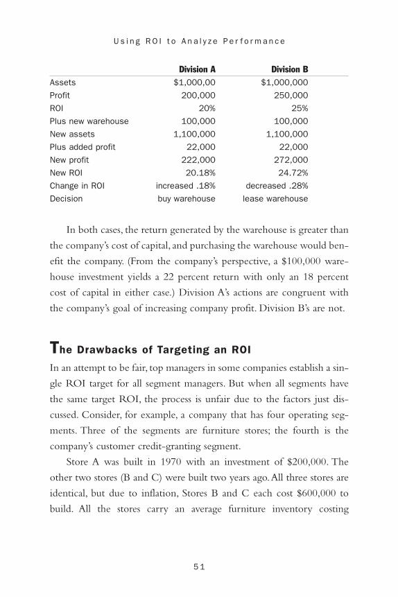
Again, assume Division A has an ROI of 20 percent, and Division B an
ROI of 25 percent.The cost of capital to the company is 18 percent and
both divisions need new warehouses that are each expected to generate
ROIs of 22 percent on the $100,000 invested.Division A will buy a ware-
house because the 22 percent return will increase the segment return, but
Division B will lease because the same return lowers its ROI.
5 1
U s i n g R O I t o A n a l y z e P e r f o r m a n c e
Division A Division BAssets $1,000,00 $1,000,000
Profit 200,000 250,000
ROI 20% 25%
Plus new warehouse 100,000 100,000
New assets 1,100,000 1,100,000
Plus added profit 22,000 22,000
New profit 222,000 272,000
New ROI 20.18% 24.72%
Change in ROI increased .18% decreased .28%
Decision buy warehouse lease warehouse
In both cases, the return generated by the warehouse is greater than
the company’s cost of capital, and purchasing the warehouse would ben-
efit the company. (From the company’s perspective, a $100,000 ware-
house investment yields a 22 percent return with only an 18 percent
cost of capital in either case.) Division A’s actions are congruent with
the company’s goal of increasing company profit. Division B’s are not.
The Drawbacks of Targeting an ROI
In an attempt to be fair, top managers in some companies establish a sin-
gle ROI target for all segment managers. But when all segments have
the same target ROI, the process is unfair due to the factors just dis-
cussed. Consider, for example, a company that has four operating seg-
ments. Three of the segments are furniture stores; the fourth is the
company’s customer credit-granting segment.
Store A was built in 1970 with an investment of $200,000. The
other two stores (B and C) were built two years ago.All three stores are
identical, but due to inflation, Stores B and C each cost $600,000 to
build. All the stores carry an average furniture inventory costing
5 2
E S S E N T I A L S o f C o r p o r a t e P e r f o r m a n c e M e a s u r e m e n t
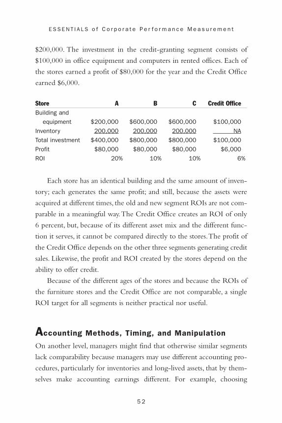
$200,000. The investment in the credit-granting segment consists of
$100,000 in office equipment and computers in rented offices. Each of
the stores earned a profit of $80,000 for the year and the Credit Office
earned $6,000.
Store A B C Credit OfficeBuilding and
equipment $200,000 $600,000 $600,000 $100,000
Inventory 200,000 200,000 200,000 NA
Total investment $400,000 $800,000 $800,000 $100,000
Profit $80,000 $80,000 $80,000 $6,000
ROI 20% 10% 10% 6%
Each store has an identical building and the same amount of inven-
tory; each generates the same profit; and still, because the assets were
acquired at different times, the old and new segment ROIs are not com-
parable in a meaningful way.The Credit Office creates an ROI of only
6 percent, but, because of its different asset mix and the different func-
tion it serves, it cannot be compared directly to the stores.The profit of
the Credit Office depends on the other three segments generating credit
sales. Likewise, the profit and ROI created by the stores depend on the
ability to offer credit.
Because of the different ages of the stores and because the ROIs of
the furniture stores and the Credit Office are not comparable, a single
ROI target for all segments is neither practical nor useful.
Accounting Methods, Timing, and Manipulation
On another level, managers might find that otherwise similar segments
lack comparability because managers may use different accounting pro-
cedures, particularly for inventories and long-lived assets, that by them-
selves make accounting earnings different. For example, choosing
5 3
U s i n g R O I t o A n a l y z e P e r f o r m a n c e
last-in, first-out (LIFO) rather than first-in, first-out (FIFO) inventory
accounting, or accelerated depreciation rather than straight-line, will
change accounting income substantially.
Other costs are subject to manipulation.A manager might delay or
eliminate some crucial but routine maintenance procedures to lower
costs and improve earnings in a slow period. Likewise, discretionary
costs such as advertising or research might be delayed or eliminated.
Production can be increased to lower the average overhead per unit,
positions that are vacated can be left unfilled, and other counterproduc-
tive measures can be taken to increase profits and ROI.
At the extreme, segment managers might falsify records, increasing
inventories to reduce cost of goods sold, or recording sales in the cur-
rent year even though they were made after the year-end cut-off.
Accounts found to be uncollectible may be retained on the books as
good receivables and spoiled or obsolete inventory included as good.
Manipulation and fraud are encouraged when top management sets
unrealistic ROI targets for segment managers.
Summary
The ROI can be analyzed as the product of two components: profit
margin and asset turnover. Profit margin expresses the percentage of
sales a company realizes in profits.A high profit margin indicates that a
company is controlling its costs relative to its sales.Asset turnover indi-
cates how much sales the company is generating relative to its assets. A
company can improve asset turnover by increasing sales or selling off
nonproductive assets. Increasing the asset turnover and/or increasing the
profit margin will increase the ROI.
From the stockholders’ point of view, the return on equity (ROE)
is a useful measure of performance. If a company increases its debt rel-
ative to its equity, the company’s leverage increases.This may have the

5 4
E S S E N T I A L S o f C o r p o r a t e P e r f o r m a n c e M e a s u r e m e n t
effect of increasing the company’s risk, but it also will cause the com-
pany’s ROE to be greater than its ROI, as long as it generates enough
income to cover additional interest expense.

CHAPTER 3
5 5
ROI and Decision Making
After read ing th is chapter, you wi l l be ab le to
• Understand how managers make decisions based on ROIand cost of capital
• Understand how managers might use variations of the ROIto improve decision making
• Understand the contribution of ROI in budgeting
• Understand the differences in assessing segment perfor-mance and assessing manager performance using ROI
• Understand issues regarding how to define the asset base,the relevant liabilities to deduct, and the appropriate valueof assets
There are some problems with using ROI for investment decisions.
A commonly cited one is the refusal of managers to pursue invest-
ments that might reduce the manager’s ROI, even though they are
otherwise acceptable. For example, a segment manager with a segment
ROI of 25 percent might refuse to invest in a project or asset expected
to return 20 percent, even if the company’s cost of capital is only 15 per-
cent, because investing in a project with a 20 percent return when the
segment’s ROI is 25 percent will lower segment ROI.

5 6
E S S E N T I A L S o f C o r p o r a t e P e r f o r m a n c e M e a s u r e m e n t
Before New Project New Project With New ProjectInvestment $1,000 $250 $1,250
Profit 250 50 300
ROI 25% 20% 24%
The same type of thinking might lead a segment manager to
increase ROI by disinvesting in assets that return less than the segment’s
ROI. Scrapping or selling otherwise profitable assets that return only 20
percent when the segment’s ROI is 24 percent increases a manager’s
ROI.
With Low ROI Project Project Scrapped Without ProjectInvestment $1,250 $250 $1,000
Profit 300 50 250
ROI 24% 20% 25%
In both cases, the project return is greater than the company’s cost
of capital and adds to the company’s total dollar profit. Now, segment
managers might not make the decision to scrap or sell lower-return
assets because top management would probably notice the sale, but top
management is less likely to notice when a segment manager passes on
an investment opportunity. Top managers often learn only of opportu-
nities disclosed to them by segment managers. If a segment manager
does not present a project to the top management, they may never learn
of it.
Both rejecting the 20 percent project and disinvesting in a 20 per-
cent asset are probably not good decisions for the company viewed as a
whole. But segment managers who do these things are acting rationally
from their own perspective, increasing the ROI of their segments. If top
5 7
R O I a n d D e c i s i o n M a k i n g
management is to avoid these situations, there must be goals for segment
managers other than a target or maximum ROI.
Profit-Neutral, Nondiscretionary Investments
Sometimes managers have to invest in things.These so-called nondiscre-
tionary investments often do not create increases in profit. Examples of
such profit-neutral investments include replacing or upgrading adminis-
trative or support facilities (such as buildings or parking lots) and adding
equipment because of OSHA regulations or EPA requirements.
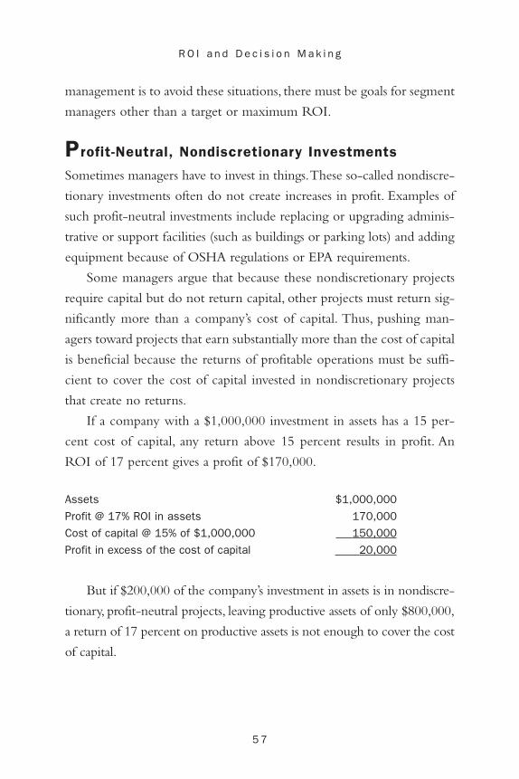
Some managers argue that because these nondiscretionary projects
require capital but do not return capital, other projects must return sig-
nificantly more than a company’s cost of capital. Thus, pushing man-
agers toward projects that earn substantially more than the cost of capital
is beneficial because the returns of profitable operations must be suffi-
cient to cover the cost of capital invested in nondiscretionary projects
that create no returns.
If a company with a $1,000,000 investment in assets has a 15 per-
cent cost of capital, any return above 15 percent results in profit. An
ROI of 17 percent gives a profit of $170,000.
Assets $1,000,000
Profit @ 17% ROI in assets 170,000
Cost of capital @ 15% of $1,000,000 150,000
Profit in excess of the cost of capital 20,000
But if $200,000 of the company’s investment in assets is in nondiscre-
tionary, profit-neutral projects, leaving productive assets of only $800,000,
a return of 17 percent on productive assets is not enough to cover the cost
of capital.
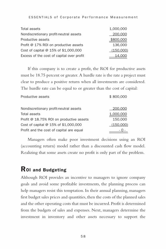
5 8
E S S E N T I A L S o f C o r p o r a t e P e r f o r m a n c e M e a s u r e m e n t
Total assets 1,000,000
Nondiscretionary profit-neutral assets 200,000
Productive assets $800,000
Profit @ 17% ROI on productive assets 136,000
Cost of capital @ 15% of $1,000,000 (150,000)
Excess of the cost of capital over profit 14,000
If this company is to create a profit, the ROI for productive assets
must be 18.75 percent or greater. A hurdle rate is the rate a project must
clear to produce a positive return when all investments are considered.
The hurdle rate can be equal to or greater than the cost of capital:
Productive assets $ 800,000
Nondiscretionary profit-neutral assets 200,000
Total assets 1,000,000
Profit @ 18.75% ROI on productive assets 150,000
Cost of capital @ 15% of $1,000,000 (150,000)
Profit and the cost of capital are equal - 0 -
Managers often make poor investment decisions using an ROI
(accounting return) model rather than a discounted cash flow model.
Realizing that some assets create no profit is only part of the problem.
ROI and Budgeting
Although ROI provides an incentive to managers to ignore company
goals and avoid some profitable investments, the planning process can
help managers resist this temptation. In their annual planning, managers
first budget sales prices and quantities, then the costs of the planned sales
and the other operating costs that must be incurred. Profit is determined
from the budgets of sales and expenses. Next, managers determine the
investment in inventory and other assets necessary to support the

5 9
R O I a n d D e c i s i o n M a k i n g
planned sales activity. Asset additions are usually budgeted using net pre-
sent values (NPV) of cash flows rather than ROI targets.
When the planning process is complete, budgeted profit divided by
the budgeted asset base determines the segment’s target ROI. But bud-
geted ROI is a target only to the extent that all the budgeted items that
compose it are targets. Budgeted ROI targets may be lower than the
actual ROI of current and past years, thus allowing managers to accept
projects with a return between the cost of capital and the segment’s ROI.
When top management uses budgets to evaluate managers, they
often assess the manager’s ability to establish a workable budget (usually
working with the manager’s superior) and then accomplish the goals the
budget describes. Segment managers can thus be evaluated by compar-
ing actual ROI to budgeted ROI instead of by ranking segment ROIs.
Budgeting that incorporates a target ROI allows top management to
consider the profit potential of each segment and allows segment man-
agers to invest in assets that increase residual income (RI), even if they
reduce ROI.
Determining Profit and the Investment Base
With RI, ROI, and other factors involved, what should segment man-
agers use to help them make investment decisions? If a company uses
ROI to evaluate segments, the segment manager will have to decide
what composition of return and investment to use. Several forms of
profit and investment can be identified, depending on the goal of the
evaluation. Is, for instance, top management evaluating the economic per-
formance of the segment or the managerial performance of the segment manager?
They are not the same thing. Economic performance evaluation of the
segment calls for classifying certain components of profit and the asset
base in a completely different manner.

6 0
E S S E N T I A L S o f C o r p o r a t e P e r f o r m a n c e M e a s u r e m e n t
If economic performance is assessed, the segment should bear all
costs directly associated with its operation and all investment dedicated
to its mission, regardless of who controls the costs or manages the invest-
ment base.The inclusion here of allocated costs is discretionary. If the
goal is to assess the manager’s performance, only the components of
profit and the investment base controlled by the manager should be
included.
Measuring Profit
Profit in published financial statements is determined using generally
accepted accounting principles (GAAP), and the performance of seg-
ments shown in published financial statements is calculated in the same
way.
Most companies provide the type of segment disclosure shown in
Exhibit 3.1, which shows segment information for Ford Motor
Company from its 2000 annual report. Ford Motor Company shows
revenues, income from continuing operations, capital expenditures,
depreciation expense, and assets for its automotive, Ford Credit, and
Hertz operations. Such detail of segment disclosure allows us to calcu-
late ROI for each of these business segments.
Ford Motor Company presents the GAAP-based information that
is useful for stockholders and others in assessing the performance of the
company’s operating segments, but it is not useful in assessing the per-
formance of segment managers. Companies that use ROI to assess the
performance of managers, rather than segments, will often exclude one
or more of the following in segment operating expenses: income taxes,
interest on corporate debt, allocated costs (of administration or other
activities), or any other costs the segment manager does not control.
Some companies argue that charging a share of interest expense to
a segment makes managers aware that invested funds are not free. If
there is no cost, some argue, segment managers might tend to use more

6 1
R O I a n d D e c i s i o n M a k i n g
funds than they otherwise would. Still, because it ignores the cost of
owners’ equity, an interest charge understates the true cost of capital,
which includes the cost of both debt and owners’ equity. (This under-
statement is in all income statements.) This causes others to insist that if
managers realize (as they do) that invested funds must recover the
unstated cost of equity capital, they also realize that the cost of creditor
capital must be recovered, even in the absence of a stated interest charge.
Determining Investment Base
There are three main questions to answer in determining the investment
amount to use in an ROI calculation:
• What assets should be included?
• What liabilities should be deducted?
• How should assets be valued?
The remainder of this chapter discusses these questions.
What Assets Should Be Included?
Deciding what assets to include will depend, in part, on whether top
management is evaluating a segment’s manager or the economic per-
formance of the segment.The issue is much the same for investment as
it is for profit. If the economic performance of the segment is assessed,
segment investment should include all capital dedicated to its mission,
regardless of who manages the investment. But if instead the segment
manager’s performance is assessed, only those components of investment
controlled by the manager should be included.
But the question is broader than defining the entity to be evaluated.
Another common problem is deciding on the treatment of shared assets.
This is a problem analogous to allocating shared expenses in determin-
ing operating income.

6 2
E S S E N T I A L S o f C o r p o r a t e P e r f o r m a n c e M e a s u r e m e n t
EXHIBIT 3 .1
Ford Motor Company Segment Disclosurefrom 2000 Annual Report
NOTE 21. Segment InformationFord has identified three primary operating segments:Automotive, Ford Credit, and Hertz. Segment selection wasbased upon internal organizational structure, the way in whichthese operations are managed and their performance evaluatedby management and Ford’s Board of Directors, the availabilityof separate financial results, and materiality considerations.Segment detail is summarized as follows (in millions):
Automotive2000
Revenues
External customer $141,230
Total Revenues $145,013
Income
Income before taxes $5,267
Provision for income tax 1,597
Income from continuing operations 3,624
Other Disclosures
Depreciation/amortization $6,497
Interest income 1,649
Interest expense 1,589
Capital expenditures 7,393
Unconsolidated affiliates
Equity in net income/(loss) (70)
Investments in 2,949
Total assets at year-end 98,157
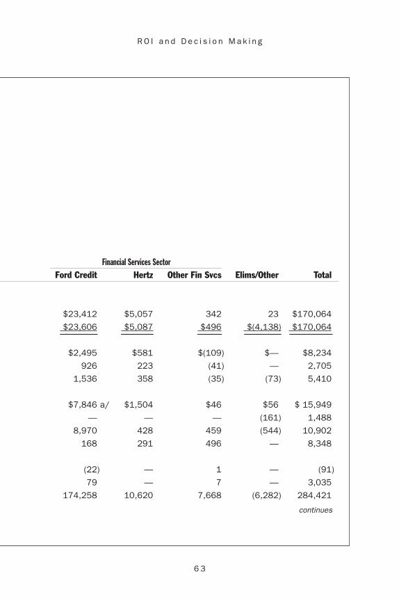
6 3
R O I a n d D e c i s i o n M a k i n g
Financial Services Sector
Ford Credit Hertz Other Fin Svcs Elims/Other Total
$23,412 $5,057 342 23 $170,064
$23,606 $5,087 $496 $(4,138) $170,064
$2,495 $581 $(109) $— $8,234
926 223 (41) — 2,705
1,536 358 (35) (73) 5,410
$7,846 a/ $1,504 $46 $56 $ 15,949
— — — (161) 1,488
8,970 428 459 (544) 10,902
168 291 496 — 8,348
(22) — 1 — (91)
79 — 7 — 3,035
174,258 10,620 7,668 (6,282) 284,421
continues

6 4
E S S E N T I A L S o f C o r p o r a t e P e r f o r m a n c e M e a s u r e m e n t
EXHIBIT 3 .1
FO R D MO T O R CO M PA N Y SE G M E N T D I S C L O S U R E C O N T I N U E D
Automotive1999
Revenues
External customer $135,073
Intersegment 4,082
Total Revenues $139,155
Income
Income before taxes $ 7,275
Provision for income tax 2,251
Income from continuing 4,986operations
Other Disclosures
Depreciation/amortization $ 5,244
Interest income 1,532
Interest expense 1,469
Capital expenditures 7,069
Unconsolidated affiliates
Equity in net income/(loss) 35
Investments in 2,539
Total assets at year-end 102,608
1998
Revenues
External customer $118,017
Intersegment 3,333
Total Revenues $121,350
Income
Income before taxes $ 5,842
Provision for income tax 1,743
Income from continuing operations 4,049
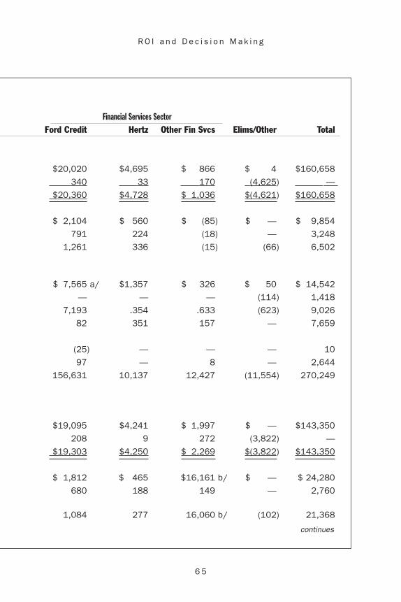
6 5
R O I a n d D e c i s i o n M a k i n g
Financial Services Sector
Ford Credit Hertz Other Fin Svcs Elims/Other Total
$20,020 $4,695 $ 866 $ 4 $160,658
340 33 170 (4,625) —
$20,360 $4,728 $ 1,036 $(4,621) $160,658
$ 2,104 $ 560 $ (85) $ — $ 9,854
791 224 (18) — 3,248
1,261 336 (15) (66) 6,502
$ 7,565 a/ $1,357 $ 326 $ 50 $ 14,542
— — — (114) 1,418
7,193 .354 .633 (623) 9,026
82 351 157 — 7,659
(25) — — — 10
97 — 8 — 2,644
156,631 10,137 12,427 (11,554) 270,249
$19,095 $4,241 $ 1,997 $ — $143,350
208 9 272 (3,822) —
$19,303 $4,250 $ 2,269 $(3,822) $143,350
$ 1,812 $ 465 $16,161 b/ $ — $ 24,280
680 188 149 — 2,760
1,084 277 16,060 b/ (102) 21,368
continues

6 6
E S S E N T I A L S o f C o r p o r a t e P e r f o r m a n c e M e a s u r e m e n t
EXHIBIT 3 .1
FO R D MO T O R CO M PA N Y SE G M E N T D I S C L O S U R E C O N T I N U E D
AutomotiveOther Disclosures
Depreciation/amortization $5,279
Interest income 1,340
Interest expense 999
Capital expenditures 7,252
Gain on spin-off of The Associates —
Unconsolidated affiliates
Equity in net income/(loss) (64)
Investments in 2,187
Total assets at year-end 85,008a/ Includes depreciation of operating leases only. Other types of depreciation/
amortization for Ford Credit are included in the Elims/Other column.b/ Includes $15,955 million non-cash gain (not taxed) on spin-off of The
Associates in the first quarter of 1998 (Note 19).
Shared assets can include a common pool of cash and receivables.
Most companies do not include shared facilities in the investment base,
but many include cash and receivables. For example, if headquarters sets
company credit policy and is responsible for collecting accounts receiv-
able, and if company cash is centrally controlled, should cash and receiv-
ables be in a segment’s assets base? Because it is difficult to determine
appropriate amounts of cash or receivables for each segment, some com-
panies include cash and receivables at arbitrary amounts, such as cash
equal to two week’s payables, or receivables equal to two month’s sales.
What Liabilities Should Be Deducted?
Regardless of the assets included, there are at least three variations of
investment created by subtracting different liabilities. Each variation
stems from a different conception of investment and results in a differ-

6 7
R O I a n d D e c i s i o n M a k i n g
Financial Services Sector
Ford Credit Hertz Other Fin Svcs Elims/Other Total
$7,327 a/ $1,212 $54 $31 $13,903
— — — (15) 1,325
6,910 318 1,114 (510) 8,831
67 317 120 — 7,756
— — 15,955 — 15,955
2 — — — (62)
76 — — — 2,263
137,248 8,873 6,181 (4,598) 232,712
ent ROI. All can be used for either the company as a whole or for
segments within the company. Exhibits 3.2a and 3.2b contain the 2000
income statement and balance sheet of Abbott Laboratories. The
amounts in the exhibits are used to calculate the three returns described
next. In each case, we use net income as the numerator.
1. Total assets. This measure deducts no liabilities and gives an ROI
sometimes called return on assets, or ROA.
Net Income $2,785,977
Divided by total assets $15,283,254
Equals an ROI (ROA) of 18.23%
2. Total assets minus current liabilities. Subtracting current liabilities
from total assets gives a return on all funds committed for the

6 8
E S S E N T I A L S o f C o r p o r a t e P e r f o r m a n c e M e a s u r e m e n t
EXHIBIT 3 .2A
Abbott Laboratories 2000 Income Statement
(in thousands)Consolidated Statement of Earnings and Comprehensive Income
(dollars and shares in thousands except per share data)
Year Ended December 31Net Sales
Cost of products sold
Research and development
Selling, general and administrative
Gain on sale of business (138,507)
Total Operating Cost and Expenses 10,345,341
Operating Earnings
Net interest expense
Income from TAP Pharmaceutical Products Inc. joint venture
Net foreign exchange (gain) loss
Other (income) expense, net 35,000
Earnings Before Taxes
Taxes on earnings 1,030.430
Net Earnings $2,785,
Basic Earnings Per Common Share $1.80
Diluted Earnings Per Common Share $1.78
Average Number of Common Shares Outstanding Used for Basic Earnings Per Common Share
Dilutive Common Stock Options 17,564
Average Number of Common Shares Outstanding Plus Dilutive Common Stock Options 1,565,579
Outstanding Common Stock Options Having No Dilutive Effect 1,038

6 9
R O I a n d D e c i s i o n M a k i n g
2000 1999 1996$13,745,916 $13,177,625 $12,512,734
6,238,646 5,977,183 5,406,635
1,351,024 1,193,963 1,228,777
2,894,176 2,657,104 2,759,757
(138,507) — —
10,345,341 10,028,250 9,395,169
3,400,575 3,149,375 3,117,565
23,221 81,765 102,540
(481,340) (390,152) (266,347)
7,287 26,238 31,158
35,000 34,636 8,349
3,816,407 3,396,888 3,241,865
1,030.430 951,129 907.512
$2,785,977 $2,445,759 $2,334,353
$1.80 $1.59 $1.52
$1.78 $1.57 $1.50
1,548,015 1,536,762 1,537,242
17,564 20,893 23,716
1,565,579 1,557,655 1,560,958
1,038 1,807 657

7 0
E S S E N T I A L S o f C o r p o r a t e P e r f o r m a n c e M e a s u r e m e n t
EXHIBIT 3 .2
AB B O T T LA B O R AT O R I E S 2000 IN C O M E STAT E M E N T C O N T I N U E D
Year Ended December 31Comprehensive Income:
Foreign currency translation adjustments
Tax benefit (expense) related to foreign currency translation adjustments
Unrealized gains (loss) on marketable equity securities
Tax benefit (expense) related to unrealized gains (loss) on marketable equity securities
Reclassification adjustment for realized gains (29,520)
Tax expense related to reclassification adjustment for realized gains
Other comprehensive income (loss), net of tax
Net Earnings 2,785
Comprehensive Income $2,588,066
Supplemental Comprehensive Income Information:
Cumulative foreign currency translation loss adjustments, net of tax $630,893
Cumulative unrealized (gains) on marketable equity securities, net of tax (27,681)
The accompanying notes to consolidated financial statements are an integral part of this statement.

7 1
R O I a n d D e c i s i o n M a k i n g
2000 1999 1996
$(198,475) $(172,517) $1,504
(476) 1,286 441
31,252 (10,548) 1,000
(12,500) 4,171 (396)
(29,520) — —
11,808 — —
(197,911) (177,608) 2,549
2,785,977 2,445,759 2,334,353
$2,588,066 $2,268,151 $2,336,902
$630,893 $431,942 $260,711
(27,681) (26,641) (33,018)

7 2
E S S E N T I A L S o f C o r p o r a t e P e r f o r m a n c e M e a s u r e m e n t
EXHIBIT 3 .2B
Abbott Laboratories Consolidated Balance Sheet
(dollars in thousands)
December 31Assets
Current Assets:
Cash and cash equivalents
Investment securities
Trade receivables, less allowances of—2000: $190,167; 1999: $238,956; 1998: $191,352
Inventories—
Finished products
Work in process
Materials
Total inventories
Prepaid income taxes
Other prepaid expenses and receivables 1,402,858
Total Current Assets 7,376,241
Investment Securities
Property and Equipment, at Cost:
Land
Buildings
Equipment
Construction in progress 330,830
Less: accumulated depreciation and amortization
Net Property and Equipment 4,816,911
Net Intangible Assets
Deferred Charges, Investments in Joint Ventures and Other AssetsLiabilities and Shareholders’ Investment
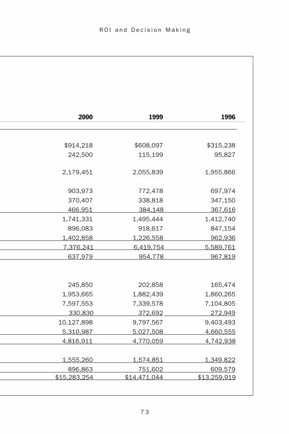
7 3
R O I a n d D e c i s i o n M a k i n g
2000 1999 1996
$914,218 $608,097 $315,238
242,500 115,199 95,827
2,179,451 2,055,839 1,955,866
903,973 772,478 697,974
370,407 338,818 347,150
466,951 384,148 367,616
1,741,331 1,495,444 1,412,740
896,083 918,617 847,154
1,402,858 1,226,558 962,936
7,376,241 6,419,754 5,589,761
637,979 954,778 967,819
245,850 202,858 165,474
1,953,665 1,882,439 1,860,265
7,597,553 7,339,578 7,104,805
330,830 372,692 272,949
10,127,898 9,797,567 9,403,493
5,310,987 5,027,508 4,660,555
4,816,911 4,770,059 4,742,938
1,555,260 1,574,851 1,349,822
896,863 751,602 609,579$15,283,254 $14,471,044 $13,259,919

7 4
E S S E N T I A L S o f C o r p o r a t e P e r f o r m a n c e M e a s u r e m e n t
EXHIBIT 3 .2B
ABBOTT LABORATORIES CONSOLIDATED BALANCE SHEET CONTINUED
December 31Current Liabilities:
Short-term borrowings and current portion of long-term debt
Trade accounts payable
Salaries, wages and commissions
Other accrued liabilities
Dividends payable
Income taxes payable
Total Current Liabilities 4,297,540
Long-Term Debt 1,076,368
Deferred Income Taxes
Other Liabilities and Deferrals 1,338,440
Shareholders’ Investment:
Preferred shares, one dollar par value Authorized—1,000,000 shares, none issued
Common shares, without par value Authorized—2,400,000,000 shares, issued at stated capital amount—Shares: 2000: 1,563,436,372; 1999: 1,564,670,440; 1998: 1,548,382,682
Common shares held in treasury, at cost—Shares: 2000: 17,502,239; 1999: 17,650,834; 1998: 17,710,838
Unearned compensation—restricted stock awards
Earnings employed in the business
Accumulated other comprehensive loss (603,212)
Total Shareholders’ Investment 8,570,906
The accompanying notes to consolidated financial statements are an
integral part of this statement.

7 5
R O I a n d D e c i s i o n M a k i n g
2000 1999 1996
$479,454 $896,271 $1,759,145
1,355,985 1,226,854 1,057,417
401,366 383,552 375,804
1,549,245 1,433,424 1,379,953
293,800 263,000 227,400
217,690 313,610 166,183
4,297,540 4,516,711 4,965,902
1,076,368 1,336,789 1,339,694
— 23,779 108,964
1,338,440 1,166,170 1,091,720
— — —
2,218,234 1,939,673 1,310,500
(255,586) (257,756) (46,735)
(18,116) (23,028) (25,796)
7,229,586 6,174,007 4,743,315
(603,212) (405,301) (227,693)
8,570,906 7,427,595 5,753,591
$15,283,254 $14,471,044 $13,259,919

7 6
E S S E N T I A L S o f C o r p o r a t e P e r f o r m a n c e M e a s u r e m e n t
long term. This measure of ROI is important to top manage-
ment, and many (but not most) companies deduct current liabil-
ities from a segment’s asset base.
Net income $2,785,977
Divided by:
Total assets $15,283,254
Minus current liabilities 4,297,540
10,985,714
Equals an ROI of 25.36%
3. Total assets minus all liabilities. This measure gives a return on net
assets or on owners’ equity, sometimes called return on equity, or
ROE. ROE is often used by shareholders or their analysts, and is
discussed further in Chapter 2.
Net income $ 2,785,977
Divided by:
Total assets $15,283,254
Minus total liabilities 6,712,348
$8,570,906
Equals an ROI (ROE) of 32.51%
Some managers of large segments might be able to borrow long-
term directly or manage their own short-term payables. Or a segment
might even be a subsidiary with full range of long- and short-term debt.
In these cases, it makes good sense to subtract from assets any debt a seg-
ment management controls. This allows the company to measure the
return on its capital invested long-term in the segment. (This is done by
a parent company that calculates its ROE in its subsidiary company.)
7 7
R O I a n d D e c i s i o n M a k i n g
Usually, however, ROA is the ROI measure best suited to invest-
ment centers because managers most often do not know or care about
the source of their funds.
How Should Assets Be Valued?
There are at least four approaches to valuing the assets included in the
investment base.
1. Gross book value.This approach uses the historical or acquisition cost
of assets,without deducting accumulated depreciation, amortization,
or depletion.
2. Net book value. Net book value of assets is gross book value minus
accumulated depreciation, amortization, and depletion.This is the
most used valuation approach.
3. Replacement cost. Replacement cost is the estimated cost of replac-
ing the assets. Replacement cost sounds logical but has defini-
tional and other problems, discussed later in the chapter.
4. Economic value. This method uses the present value of future cash
flows.Almost no one uses economic value.
Gross Book Value
Using the gross book value of the assets in the investment base gives
managers an incentive to make unwise equipment disposal and replace-
ment decisions.
Disposal Decisions.
Managers who are evaluated by an ROI using gross book values have
an incentive to (1) scrap old equipment that is fully depreciated, infre-
quently used, but still needed, and (2) scrap any equipment that is not

7 8
E S S E N T I A L S o f C o r p o r a t e P e r f o r m a n c e M e a s u r e m e n t
returning a target ROI, regardless of condition. Even if scrapping equip-
ment is foolish from the company’s viewpoint and produces a loss on
disposal for the segment, the disinvestment still improves the segment’s
ROI because it reduces the investment base (the denominator).The dis-
posal will improve ROI even in the year of disposal if the loss on dis-
posal is less than the disposed asset’s profit shortfall.
For example, Segment X has a piece of equipment, A, that returns
less than the other assets, as follows.
SEGMENT XEquipment A All Other Assets Total for Segment
Gross BV $100,000 $500,000 $600,000
Profit 15,000 125,000 140,000
ROI 15% 25% 23.33%
Equipment A has a profit shortfall of $10,000. (A profit of $10,000
more, or $25,000, gives a return of 25 percent, equal to the return of the
other assets.) Thus, if the loss on disposal of Equipment A is less than
$10,000, segment ROI in the year of disposal is increased. If Equipment
A is sold for a $5,000 loss on January 1 (before Equipment A makes any
profit contribution), segment ROI still increases from 23.33 percent to
24 percent in the year of disposal, despite the loss of $15,000 profit the
equipment would have earned if not disposed of.
SEGMENT XEquipment A All Other Assets
Gross BV – 0 – $500,000
Profit before loss – 0 – 125,000
Disposal loss (5,000)
Profit after loss 120,000
ROI 24%

7 9
R O I a n d D e c i s i o n M a k i n g
In subsequent years, with Equipment A and its contribution to profit
gone, the Segment X operating profit is reduced by $15,000 per year, but
ROI is increased to 25 percent due to the reduced investment base.
SEGMENT XAll Other Assets
Gross BV $500,000
Profit 125,000
ROI 25%
The effect of valuing the asset base at gross book value is generally
dysfunctional.The segment manager would be motivated to dispose of
Equipment A even if its 15 percent return was above the cost of capi-
tal.The manager would be motivated to dispose of the equipment even
if it were fully depreciated and its net book value was zero.
Replacement Decisions.
When assets are replaced, the company must invest an amount equal to
the cost of the new asset minus the salvage value of the old asset. But
the use of gross book value as the segment’s investment value causes its
assets to increase by only the difference between the cost of the new
asset added to the books and the cost of the old asset removed.To the
segment manager, this means that the additional investment to obtain
new assets is quite small, and replacement investments can be made
(from the segment manager’s perspective) at far, far less than the cutoff
rate used in cash flow models.
For example, if a manager acquires a new asset for $45,000 to
replace one that cost $35,000, the manager may pay $45,000, but the
increase in the gross book value of the investment base is only $10,000
8 0
E S S E N T I A L S o f C o r p o r a t e P e r f o r m a n c e M e a s u r e m e n t
(investment base + $45,000 � $35,000 = new investment base). The
increase is the same here whether the old asset is relatively new or com-
pletely depreciated, because it is the gross book value of the old machine
that is counted in the investment base.
If segment earnings then increase by $2,000, the additional invest-
ment appears to earn a return of $2,000/$10,000, or 20 percent. But if
the old asset was only worth $5,000 as a trade-in, the cash investment
required is actually $40,000, and the average return only $2,000/
$40,000, or 5 percent.
Net Book Value
Net book value is the value at which an asset is carried in the books (the
accounting records). Net book value is original cost minus any cost
already depleted, amortized, or depreciated. For instance, a building that
cost $500,000 and on which $100,000 in depreciation expense had
been taken has a book value of $400,000. Net book value, in companies
with one asset or assets of a similar age, gives a decreasing investment
base.This effect is increased when accelerated depreciation methods are
used. Because the net book value of an asset is less each year, ROI
increases each year. This effect misleads segment managers and may
cause them to avoid investing in new assets.
Suppose a segment has an investment of $200,000 and net income
of $30,000, as follows. ROI is 15 percent ($30,000/$200,000).
Investment:Cash $20,000
Inventory 30,000
Plant and equipment 150,000
Total investment in assets $200,000
Net income $30,000
ROI 15%
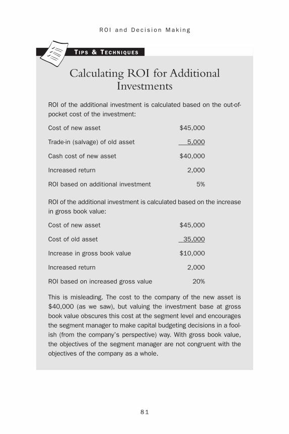
8 1
R O I a n d D e c i s i o n M a k i n g
Calculating ROI for AdditionalInvestments
ROI of the additional investment is calculated based on the out-of-pocket cost of the investment:
Cost of new asset $45,000
Trade-in (salvage) of old asset 5,000
Cash cost of new asset $40,000
Increased return 2,000
ROI based on additional investment 5%
ROI of the additional investment is calculated based on the increasein gross book value:
Cost of new asset $45,000
Cost of old asset 35,000
Increase in gross book value $10,000
Increased return 2,000
ROI based on increased gross value 20%
This is misleading. The cost to the company of the new asset is$40,000 (as we saw), but valuing the investment base at grossbook value obscures this cost at the segment level and encouragesthe segment manager to make capital budgeting decisions in a fool-ish (from the company’s perspective) way. With gross book value,the objectives of the segment manager are not congruent with theobjectives of the company as a whole.
T I P S & TE C H N I Q U E S

8 2
E S S E N T I A L S o f C o r p o r a t e P e r f o r m a n c e M e a s u r e m e n t
EXHIBIT 3 .3
Increasing ROI Using Net Book Value
End of Assets at Annual Year Cost Depreciation
1 $200,000 $30,000
2 200,000 30,000
3 200,000 30,000
4 200,000 30,000
5 200,000 30,000
Even if the segment keeps exactly the same assets and earns exactly
the same profit each year, ROI will not remain 15 percent because the
plant and equipment are depreciated each year. Assume the plant and
equipment have a life of five years and that depreciation expense of
$30,000 ($150,000/5 years) is taken each year. Depreciation expense is
charged against earnings each year and the book value of the investment
is reduced to zero over the asset’s life.
If cash, inventory, and profit remain the same, the net book value of
the segment investment and the ROI calculated on the book value is as
shown in Exhibit 3.3. ROI is based on net book value at the end of each
year, and increases from 17.6 percent at the end of year one to 60 per-
cent at the end of year five when the plant and equipment are fully
depreciated (net book value = zero).The 15 percent ROI occurs only
in year one, and only if the net book value of assets at the beginning of
the year is used. By the end of the year, the book value has been
decreased by the depreciation expense and the ROI has increased.

8 3
R O I a n d D e c i s i o n M a k i n g
AccumulatedDepreciation
to Date Book Value Profit ROI%$30,000 $170,000 $30,000 17.6
60,000 140,000 30,000 21.4
90,000 110,000 30,000 27.3
120,000 80,000 30,000 37.5
150,000 50,000 30,000 60.0
This effect (increasing ROI) occurs in companies with only one
asset or companies that purchase all their assets in the same year.When
a company purchases assets in different years, the distortion is still pre-
sent but averages out and is apparent.Additionally, when ROI is calcu-
lated using net book value at the beginning of the year, it is different
from ROI calculated using book value at the end of the year. Some
companies attempt to overcome this by using the average of beginning
and ending book values. In our example, we can calculate the following
equally acceptable ROIs for year one.
Using beginning of year book value $30,000/$200,000 ROI = 15.0%
Using end of year book value $30,000/$170,000 ROI = 17.6%
Using average book value for year $30,000/$185,000 ROI = 16.2%
This problem can be avoided by using replacement cost and annu-
ity depreciation. Annuity depreciation uses a mathematical procedure
8 4
E S S E N T I A L S o f C o r p o r a t e P e r f o r m a n c e M e a s u r e m e n t
that results in larger depreciation charges as the asset ages. It is cumber-
some to apply and produces a pattern of depreciation expense that does
not match the way assets wear out. Accountants always mention annu-
ity depreciation when discussing this problem, but we know of no com-
pany that uses annuity depreciation.
Replacement Value
Replacement cost is defined several different ways.Assume one segment
of a company uses computerized printing equipment that cost $140,000
when purchased five years ago.The equipment has a seven-year life, is
depreciated $20,000 per year, and after five years has a net book value
of $40,000 [$140,000 � (5 � $20,000)]. Its replacement cost can be
estimated using at least four approaches, each leading to a different
value.
Replacement Value As Is.
This is the cost of replacing the equipment with used equipment in the
same condition. If there is no used equipment market and the equip-
ment to be valued is unique, replacement value can be difficult to esti-
mate. Assume used equipment in the same condition is in demand for
use as parts in repairing old processes and costs $60,000 (the amounts in
this example are for illustration only).
Replacement Value New.
The cost of replacing the equipment with new equipment of exactly
the same model and type is $200,000. Because the equipment is old,
new equipment exactly like the old equipment does not exist and
requires expensive, custom manufacture. Equipment using computer

8 5
R O I a n d D e c i s i o n M a k i n g
chips two or three generations old is frequently no longer manufac-
tured.
Capacity Replacement Value.
The cost of replacing not the equipment but the capacity of the equip-
ment with equipment currently manufactured is the capacity replace-
ment value. For computerized equipment, new technology often makes
it less expensive to purchase the same capacity each year. New equip-
ment that can perform the same work as the old printing equipment
costs $90,000.
Price-Level Adjusted Historical Cost.
Although not a true measure of replacement cost, some companies
adjust an asset’s cost for changes in prices to estimate a current cost. If
the price index changed from 110 to 165 during the five years the com-
pany has owned the equipment, the price-level adjusted cost of the
equipment is $140,000 � 165/110 = $210,000.
Even when a definition of replacement cost is chosen, a company
may have great difficulty obtaining annual replacement value estimates
of the collections of assets that make up the factories, stores, and other
operating investments of each segment. Estimates by consultants or
appraisers are often subjective and may vary widely.
Economic Value
The economic value is the present value of an asset’s future cash flows.
It is subjective and difficult to determine.To estimate economic value,
managers must both estimate the future cash flows and decide on an
appropriate discount rate. These estimated flows must be the flows
expected to occur, not the flows managers might target or aspire to.

8 6
E S S E N T I A L S o f C o r p o r a t e P e r f o r m a n c e M e a s u r e m e n t
These expected actual cash flows are then discounted to their present
value.
This process produces a conflict between determining the eco-
nomic value of the investment from predictions of the segment man-
ager’s performance, and evaluating the segment manager’s performance
using the profit generated and the present value of top management’s
predictions. Performance is, in effect, evaluated against an estimate of
itself.
Additionally, the economic value approach gives the same value to
an asset, regardless of how it was obtained, wisely or otherwise. If a man-
ager saves on an equipment acquisition by shopping wisely or building
the asset in-house, the manager is assigned the same dollar investment
base as another manager who acts foolishly and buys identical equip-
ment at a high price (assuming the estimated cash flows and discount
rate are the same). Since ROI is supposed to improve a segment man-
agement’s motivation and top management’s evaluation procedures, this
is a serious problem.
To illustrate, assume two retail stores in Kansas City are owned by
C. C. Smith, who wishes to value the assets of the two store managers
using the economic value approach. Coincidentally, Smith decides the
stores should begin delivering to customers and directs the managers to
purchase one delivery truck each and begin this service as economically
as possible. Smith estimates the cash flows from the delivery service will
be $10,000 per year, and the trucks will each last five years. Smith
believes the appropriate discount rate is 10 percent.
One store manager shops wisely and purchases a new truck with the
minimum basic equipment for $24,000.The other manager understands
the economic value method and buys a top-of-the-line truck loaded
with options for $40,000.What value is placed on each manager’s truck?
The present value of $10,000 each year for five years at 10 percent is
8 7
R O I a n d D e c i s i o n M a k i n g
3.791 � $10,000 = $37,910.Thus, the investment base of each manager
is increased by $37,910, the economic value of the truck.
Finally, managers resist the use of economic value.They do not like
to be evaluated with artificial measures concocted by economists. As a
result, economic value is not often used to value the investment base in
ROI measures.
Summary
Managers can use ROI to make decisions about which assets to acquire
and which to sell.The decision process involves deciding how to mea-
sure return and how to measure the asset base that would be assumed
to generate the return. It is important to define these in a way that is
appropriate to the evaluation of segment performance versus the evalu-
ation of management performance. Methods for valuing assets include
gross book value, net book value, replacement cost, and economic value.


8 9
CHAPTER 4
Variations of ROI
After read ing th is chapter, you wi l l be ab le to
• Understand the gross margin return on investment(GMROI)
• Understand the components of the GMROI
• Understand the differences between the GMROI and the ROI
• Understand how to improve the GMROI
• Understand the contribution margin return on investment(CMROI)
• Understand the nature of fixed costs and variable costs
• Understand the difference in the contribution marginincome statement and the gross profit income statement
• Be able to compare the CMROI and the GMROI to the ROI
• Understand the relationship between cash flow and qualityof earnings
• Understand the cash return on investment
Gross Margin Return on Investment (GMROI)
There are several variations of ROI. One is called gross margin return on
investment (GMROI), and it examines the relationship between the gross

9 0
E S S E N T I A L S o f C o r p o r a t e P e r f o r m a n c e M e a s u r e m e n t
margin on sales and the investment in inventory required to support the
sales. GMROI is gross margin in dollars for some period divided by the
average cost of inventory on hand during the same period.
The numerator, gross margin, is sales minus the cost of goods
(inventory) sold. Sales of $1,000 and cost of goods sold of $600 yield a
gross margin of $400. This calculation is often made in the first three
lines of the income statement.
Sales $1,000
Cost of goods sold 600
Gross margin $ 400
If the $1,000 in sales requires an average inventory equal to two
months’ cost of sales ($600/12 � 2 months or $100), GMROI is 400
percent, or $4 for every $1 invested in inventory.
Comparing GMROI and ROI
GMROI differs from ROI in two ways: GMROI uses gross margin
instead of net income as the return (gross margin is simply higher up
than net income on the income statement), and it considers only the
investment in inventory. Since net income is usually small relative to a
company’s total investment in assets, ROI calculated using a company’s
net income and total assets is almost always less than 20 percent. But
gross margin is substantially larger than net income.And average inven-
tory is generally much smaller than total assets. Because of this, GMROI
is often quite large relative to ROI.
GMROI �gross margin
average inventory 1at cost 2 �$400$100
� 400%
GMROI �gross margin
average inventory 1at cost 2
9 1
Va r i a t i o n s o f R O I
Managers believe gross margin and the gross margin percentage are
important measures. When managers say, “We make a dollar on each
shirt sold,” they typically mean,“We sell each shirt for a dollar more than
its cost.” If a shirt that costs $2 is sold for $3, the gross margin is $1.The
gross margin percentage is 33.3 percent, calculated by dividing gross
margin by the selling price ($1/$3).
Net income is determined by subtracting cost of goods sold and all
other expenses from sales.The net income created on the sale of each
shirt might be only $0.20 after the costs of salespeople, supervision, rent,
utilities, advertising, and other costs are subtracted from gross margin.
Gross margin must be large enough to cover all these other expenses or
the company will incur a loss.
Components of GMROI
Like ROI, GMROI can be broken into margin and turnover compo-
nents. GMROI = Gross margin on sales � Inventory turnover. The
margin component of GMROI is the percentage gross margin on sales.
For the example, gross margin on sales is 40 percent.
The turnover component is inventory turnover using sales as the
numerator.An alternative calculation for inventory turnover uses cost of
goods sold as the numerator.
Combining these components shows how they interact to give a
GMROI of 400 percent. A change in either component, margin or
turnover, changes GMROI.
Inventory turnover �sales
inventory�
$1,000$100
� 10 times
Gross marginon sales
�gross margin
sales�
$400$1,000
� 40%
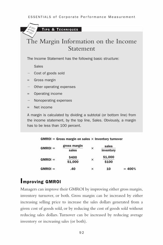
9 2
E S S E N T I A L S o f C o r p o r a t e P e r f o r m a n c e M e a s u r e m e n t
The Margin Information on the IncomeStatement
The Income Statement has the following basic structure:
Sales
� Cost of goods sold
= Gross margin
� Other operating expenses
= Operating income
� Nonoperating expenses
= Net income
A margin is calculated by dividing a subtotal (or bottom line) fromthe income statement, by the top line, Sales. Obviously, a marginhas to be less than 100 percent.
T I P S & TE C H N I Q U E S
Improving GMROI
Managers can improve their GMROI by improving either gross margin,
inventory turnover, or both. Gross margin can be increased by either
increasing selling price to increase the sales dollars generated from a
given cost of goods sold, or by reducing the cost of goods sold without
reducing sales dollars. Turnover can be increased by reducing average
inventory or increasing sales (or both).
� 400%10�.40GMROI �
$1,000$100
�$400
$1,000GMROI �
salesinventory
�gross margin
salesGMROI �
Inventory turnover�Gross margin on salesGMROI �

9 3
Va r i a t i o n s o f R O I
Increasing Gross Margin
For retailers, the selling price and the cost of inventory sold are often set
by market forces.A retail store must sell at competitive prices and often
must buy its inventory from the same sources that supply its competi-
tion. Consequently, a retail store that seeks to change its gross margin
must negotiate discounts for buying in large quantities or for buying
much of its inventory from the same vendor.
Manufacturers have more opportunities to work toward lower costs
than do retailers. Manufacturing costs are composed of three compo-
nents: raw materials, labor, and overhead. Managers can often lower the
cost of manufactured inventory by negotiating lower costs on materials,
by automating processes to reduce labor, or by adopting one of the
newer manufacturing techniques such as using robotics or just-in-time
manufacturing.
In our earlier example, GMROI is 400 percent. If management
increases selling prices by 10 percent (from $1,000 to $1,100) with no
loss in volume, gross margin percentage is increased to .4545 (a repeat-
ing decimal), turnover is increased to 11, and GMROI is increased to
500 percent, or $5 for every $1 invested in inventory.
Original performance:
Improved performance (10% increase in sales dollars):
� 500%11�.4545GMROI �
$1,100$100
�$500
$1,100GMROI �
� 400%10�.40GMROI �
$1,000$100
�$400
$1,000GMROI �
GMROI �gross margin
sales�
salesinventory
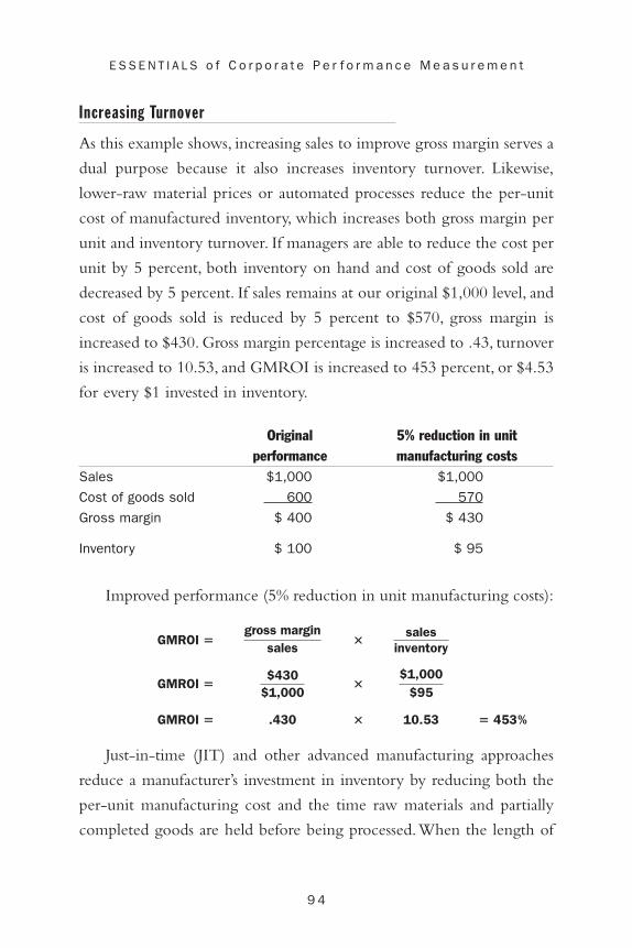
9 4
E S S E N T I A L S o f C o r p o r a t e P e r f o r m a n c e M e a s u r e m e n t
Increasing Turnover
As this example shows, increasing sales to improve gross margin serves a
dual purpose because it also increases inventory turnover. Likewise,
lower-raw material prices or automated processes reduce the per-unit
cost of manufactured inventory, which increases both gross margin per
unit and inventory turnover. If managers are able to reduce the cost per
unit by 5 percent, both inventory on hand and cost of goods sold are
decreased by 5 percent. If sales remains at our original $1,000 level, and
cost of goods sold is reduced by 5 percent to $570, gross margin is
increased to $430. Gross margin percentage is increased to .43, turnover
is increased to 10.53, and GMROI is increased to 453 percent, or $4.53
for every $1 invested in inventory.
Original 5% reduction in unit performance manufacturing costs
Sales $1,000 $1,000
Cost of goods sold 600 570
Gross margin $ 400 $ 430
Inventory $ 100 $ 95
Improved performance (5% reduction in unit manufacturing costs):
Just-in-time (JIT) and other advanced manufacturing approaches
reduce a manufacturer’s investment in inventory by reducing both the
per-unit manufacturing cost and the time raw materials and partially
completed goods are held before being processed.When the length of
� 453%10.53�.430GMROI �
$1,000$95
�$430
$1,000GMROI �
salesinventory
�gross margin
salesGMROI �

9 5
Va r i a t i o n s o f R O I
time inventories are held is reduced, the average investment in invento-
ries is reduced.
To illustrate, our original example assumed cost of goods sold to be
$600,000 and an average inventory on hand equal to two months’ cost
of sales ($600,000/12 = $50,000/month � 2 = $100,000). If JIT and
other measures allowed management to reduce inventory between
processes to only one-half of one month’s cost of sales, ($600,000/12 =
$50,000/month � .50 = $25,000), turnover is increased to 40, and
GMROI increases to 1600 percent, or $16 for each dollar of investment
in inventory.
For a competitor who does not adopt a JIT approach to manufac-
turing, an equivalent GMROI is impossible.Assume a competitor who
has not adopted JIT has identical sales and still requires two months’ cost
of sales to remain in inventory.Turnover is still 10 (as in our original cal-
culation), and to generate a GMROI of 1600 percent, gross margin per-
centage must be 160 percent, requiring gross margin to be greater than
sales! Such a result is impossible.
Gross margin percentage must be 160 percent.
� 1600%10�1.60GMROI �
$1,000$100
�?
$1,000GMROI �
salesinventory
�gross margin
salesGMROI �
� 1600%40�.40GMROI �
$1,000$25
�$400
$1,000GMROI �
salesinventory
�gross margin
salesGMROI �

9 6
E S S E N T I A L S o f C o r p o r a t e P e r f o r m a n c e M e a s u r e m e n t
Including Markup in GMROI
The analysis of financial ratios is more an art than a science.There-
fore, analysts may use different variations of the ratios. Instead of deter-
mining inventory turnover with sales as the numerator (as shown
previously),we can use cost of goods sold as the numerator and expand the
components to include markup. In our original example, markup on cost
is 166.7 percent and inventory turnover using cost of goods sold is 6.0.
Combining these new components shows how they interact to
explain a GMROI of 400 percent. GMROI is not changed by using
these new components, but a change in any component, margin,
markup, or turnover changes GMROI.
Markup is the factor that drives gross margin: Higher markups pro-
duce higher gross margins. Including markup in the components gives
added flexibility to managers trying to increase GMROI. When the
relationships are presented in this form, managers see that they can
improve GMROI by increasing either gross margin, markup, or inven-
tory turnover.
� 400%6�1.667�.40GMROI �
$600$100
�$1,000$600
�$400
$1,000GMROI �
cost of goods soldinventory
�sales
cost of goods sold�
gross marginsales
GMROI �
inventory turnover�markup�gross marginGMROI �
� 6 times$600$100
�cost of goods sold
inventoryInventory turnover �
� 166.7%$1,000$600
�sales
cost of goods soldMarkup on cost �

9 7
Va r i a t i o n s o f R O I
Types of Costs
When a manufacturer produces more than it sells and thus increases the
number of units it keeps in inventory, some costs assigned to the
increased inventory are real costs that require additional current expen-
ditures and some are not.Additional electricity is consumed and assem-
bly employees work more hours for which they must be paid.These are
real cost increases. Other costs assigned to inventory are not-so-real
costs that do not require additional current expenditures. These costs
consist either of allocations (assignments) of costs incurred in prior
years, such as depreciation on a plant, or costs that would be spent in the
same amount even if production had not increased, such as the cost of
fire insurance or property taxes.
Fixed Costs
Fixed costs are costs that do not change in total when a company’s activ-
ity level changes. If depreciation on the factory building is $60,000 per
month, it remains $60,000 per month regardless of whether the factory
operates one shift or three. If production increases from 10,000 units for
one shift to 60,000 units for three, the average depreciation cost per unit
decreases from $6 per unit ($60,000/10,000 units), to $1 per unit
($60,000/60,000 units) but total depreciation cost does not change.
Thus, there is no incremental (or increased) fixed cost associated with
increased activity. Fixed costs for a manufacturer are generally not the
costs of production but are instead the costs of maintaining the capac-
ity to produce.
Variable Costs
Variable costs are costs that do change in total when a company’s activity
level changes.Variable costs for a manufacturer include the costs of mate-
rials, labor, and some overhead (called direct overhead), such as electric-
ity consumed and the maintenance of equipment. If $20 of raw material

9 8
E S S E N T I A L S o f C o r p o r a t e P e r f o r m a n c e M e a s u r e m e n t
Z is needed to produce one unit of product, the total cost of raw mate-
rial Z is $200,000 when 10,000 units are produced ($20 � 10,000 units)
but $600,000 when 30,000 units are produced ($20 � 30,000 units).
A variable cost is an incremental (or increased) cost associated with
increased activity.The increased cost of producing an additional order is
sometimes called the marginal cost of producing the order. In our exam-
ple, the variable cost per unit for raw materials remains the same ($20),
but total costs vary directly with activity. The marginal cost of produc-
ing an additional 100 units is $2,000 (100 units � $20).
Contribution Margin Return on Investment (CMROI)
We have discussed the usefulness of gross margin in assessing profitabil-
ity, but many managers avoid gross margin and use contribution margin
instead in their decision making. The contribution margin return on
investment (CMROI) is a refinement of the gross margin return on
investment (GMROI). CMROI is often more appropriate for assessing
performance or making decisions because it recognizes that costs are not
all the same. Unlike gross margin, contribution margin is generally not
available to persons outside a company.
CMROI examines the relationship between the contribution mar-
gin on sales and the incremental investment in inventory required to
support the sales. Contribution margin is calculated by subtracting total
variable costs from sales. CMROI uses a contribution margin subtotal
sometimes called manufacturing margin or manufacturing contribution mar-
gin, calculated by subtracting only variable manufacturing costs (as in
variable cost of goods sold) from sales. Variable costs of selling and
administration, such as commissions or collections, are then subtracted
from manufacturing contribution margin to get contribution margin.
Manufacturing contribution margin and contribution margin are
calculated as shown in the contribution margin formatted income state-

9 9
Va r i a t i o n s o f R O I
EXHIBIT 4 .1
Contribution Margin and Gross ProfitFormatted Income Statements
Bunchy Company Contribution Margin Income Statement for the year
ended December 31, 200X
Sales $500,000
Variable cost of goods sold 150,000
Manufacturing contribution margin 350,000
Variable selling costs $ 25,000
Variable administrative costs 50,000 75,000
Contribution margin 275,000
Fixed costs:
Manufacturing $150,000
Selling 37,500
Administrative 12,500 200,000
Net income $75,000
Bunchy Company Gross Profit Income Statement for the year ended
December 31, 200X
Sales $500,000
Cost of goods sold 300,000
Gross profit 200,000
Selling costs $62,500
Administrative costs 62,500 125,000
Net income $75,000
ment in Exhibit 4.1. Exhibit 4.1 also contains a gross profit formatted
or multiple-step income statement. With additions for selling and
administrative costs, both income statements contain figures from the
main example used throughout the last chapter.
If $500,000 in sales (from Exhibit 4.1) requires an average invest-
ment in the variable cost of inventory equal to two months’ variable

1 0 0
E S S E N T I A L S o f C o r p o r a t e P e r f o r m a n c e M e a s u r e m e n t
cost of sales ($150,000/12 = $12,500 � 2), or $25,000, CMROI is 1400
percent, or $14 for every $1 invested in the variable cost of inventory.
Two-Component CMROI Analysis
Like ROI or GMROI, CMROI can be broken into margin and
turnover components. The margin component of CMROI is the man-
ufacturing contribution margin percentage. In our example, manufac-
turing contribution margin is 70 percent.
As with GMROI, the turnover component is inventory turnover,
but now the variable cost of inventory is the denominator.
These components combine to give the CMROI.
Three-Component CMROI Analysis
As with GMROI, CMROI can be broken into three components if we
calculate inventory turnover using the variable cost of sales (rather than
� 1400%20�.70CMROI �
salesinventory
variable cost
�
manufacturingcontribution margin
salesCMROI �
inventoryturnover
�manufacturing
contribution marginCMROI �
Inventory turnover �sales
inventory�
$500,000$25,000
� 20 times
Manufacturingcontribution
margin%�
manufacturing CMsales
�$350,000$500,000
� 70%
CMROI �
manufacturingcontribution marginaverage inventory1at variable cost 2
�$350,000$25,000
� 1400%

1 0 1
Va r i a t i o n s o f R O I
sales). The three components generated are margin, markup, and
turnover. The margin component of CMROI is the manufacturing
contribution margin percentage, as calculated previously. Markup and
turnover both use variable cost of goods sold.
These three components combine to give the CMROI.
Comparing CMROI and GMROI
The excess of sales over variable cost of goods sold is a better measure of
the benefit of selling more inventory than the excess of sales over the full
cost of goods sold. Likewise, the variable cost of units placed in inventory
is a better measure of the investment required to maintain an inventory.
Because fixed costs do not change in total when inventory is increased or
decreased, they are usually irrelevant to decisions and should not be in
ratios used to evaluate managerial performance.
Because contribution margin affects income so much more directly
than gross margin, CMROI is a much more valuable analysis tool than
GMROI.Contribution margin can be increased by either increasing sell-
ing price or reducing variable costs. Decreasing a bookkeeping allocation
of fixed cost to cost of goods sold increases GMROI but does not change
� 1400%6�3.333�.70CMROI �
variable costof goods sold
inventory�
salesvariable cost of goods sold
�manufacturing CM
salesCMROI �
inventoryturnover
�markup�manufacturing CM%CMROI �
� 6 times$150,000$25,000
�
variable costof goods sold
inventory�
Inventoryturnover
� 333.3%$500,000$150,000
�sales
variable costof goods sold
�markup

1 0 2
E S S E N T I A L S o f C o r p o r a t e P e r f o r m a n c e M e a s u r e m e n t
CMROI. Because bookkeeping allocations of fixed costs do not change
total costs in any way, it makes sense that CMROI does not change.
Cash Return on Investment
So far we have discussed ROI calculated using net income, gross profit,
and manufacturing contribution margin. Now we are going to look at
an ROI variation that defines return as cash inflow from operations.
Cash Flow and Quality of Earnings
Operating cash inflow is the most rigorous measure of return on invest-
ment that we can take.To stockholders and other investors, income is of
high quality only if it is accompanied by an appropriate cash inflow.
Income not accompanied by cash inflow is perceived to be of low qual-
ity. Low-quality earnings result in a lower market value for a company’s
stock because analysts believe that earnings accompanied by cash flows
are worth more than earnings that are not.
Low quality also results when earnings cannot be sustained or when
accounting procedures increase earnings without a corresponding increase
in cash flow. High-quality earnings can be sustained and are accompanied
by appropriate cash inflows.
Earnings are not accompanied by sustainable cash flows when man-
agers attempt to increase earnings by changing the timing of revenues
and expenses. For example, managers might avoid some maintenance
procedures to reduce expenses and raise income. If maintenance costing
$50,000 is put off until next year, profits this year are improved by
$50,000 but earnings next year are reduced by the same amount.
Likewise,managers might try to increase sales this year by relaxing credit
standards, creating sales that benefit the current year but that are more
likely to become bad debts in the following year.

1 0 3
Va r i a t i o n s o f R O I
Investors also downgrade the quality of earnings when a company
chooses an accounting method because it maximizes reported earnings.
Companies that use straight-line depreciation or FIFO inventory are
perceived to have lower-quality earnings than a company that uses an
accelerated depreciation method or LIFO inventory.2 (Both straight-
line depreciation and FIFO inventory increase reported earnings rela-
tive to companies that use an accelerated depreciation method or LIFO
inventory.)
Cash ROI
Cash ROI is determined by dividing cash flow from operations during
a period by the average investment in total assets during the same
period. If average assets are $400,000 and cash from operations is
$20,000, cash ROI is 5 percent.
Like other variations of ROI, cash ROI can be divided into a return
on sales component and a turnover component. The return on sales
component is cash return on sales, and the turnover is the turnover of
total investment in assets. If sales are $500,000, cash return on sales is 4
percent and asset turnover is 1.5.
� .051.25�.04Cash ROI �
$500,000$400,000
�$20,000$500,000
Cash ROI �
salesaverage assets
�
cash flowfrom operations
salesCash ROI �
asset turnover�cash return on salesCash ROI �
Cash ROI �cash flow from operations
average total assets�
$20,000$400,000
� .05

1 0 4
E S S E N T I A L S o f C o r p o r a t e P e r f o r m a n c e M e a s u r e m e n t
Cash return on sales is a cash flow ratio similar to the profitability
ratio, return on sales (i.e., net income/sales). Cash return on sales helps
investors evaluate the quality of a company’s earnings and determine the
extent it can support its net income with cash flow.
The asset turnover ratio measures management’s effectiveness in
using the company’s total assets to generate sales activity.
Estimating Cash Flow from Operations
Cash flow from operations is shown in every published cash flow state-
ment. Still, it is common for people to estimate it from net income by
adding depreciation and amortization expense to net income. Cash is
consumed when a company purchases an asset such as a plant or a patent,
but no cash flow occurs when the cost of the asset is depreciated or
amortized against earnings each year. Depreciation and amortization
expenses are allocations of an asset’s original cost to a period benefited
by the asset’s use.Because of this, depreciation and amortization are oper-
ating expenses that do not require operating cash outflows each year.
Because these two operating expenses subtracted in the income
statement do not require cash outflows, many people think that adding
them back to net income gives a good approximation of cash from
operations. Exhibits 4.2 and 4.3 show the 2000 income statement for
Bristol-Myers Squibb Company. We estimate cash from operations by
adding Bristol-Myers depreciation of $746,000,000 to its net income of
$4,711,000,000. Bristol-Myers’s cash flow from operations is estimated
to be $5,457,000,000. In Exhibit 4.4 Bristol-Myers’s statement of cash
flows shows net cash from operating activities as $4,652,000,000.
The statement of cash flows published in a company’s annual report
shows cash flow, in or out, for three separate activities: operating, financ-
ing, and investing.Two methods may be used in the statement of cash
flows to determine and present cash flow from operating activities: the
direct method and the indirect method.
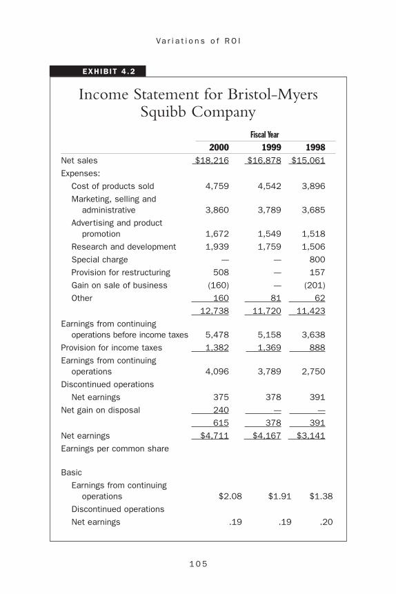
1 0 5
Va r i a t i o n s o f R O I
EXHIBIT 4 .2
Income Statement for Bristol-MyersSquibb Company
Fiscal Year
2000 1999 1998Net sales $18,216 $16,878 $15,061
Expenses:
Cost of products sold 4,759 4,542 3,896
Marketing, selling and administrative 3,860 3,789 3,685
Advertising and product promotion 1,672 1,549 1,518
Research and development 1,939 1,759 1,506
Special charge — — 800
Provision for restructuring 508 — 157
Gain on sale of business (160) — (201)
Other 160 81 62
12,738 11,720 11,423
Earnings from continuing operations before income taxes 5,478 5,158 3,638
Provision for income taxes 1,382 1,369 888
Earnings from continuing operations 4,096 3,789 2,750
Discontinued operations
Net earnings 375 378 391
Net gain on disposal 240 — —
615 378 391
Net earnings $4,711 $4,167 $3,141
Earnings per common share
Basic
Earnings from continuing operations $2.08 $1.91 $1.38
Discontinued operations
Net earnings .19 .19 .20
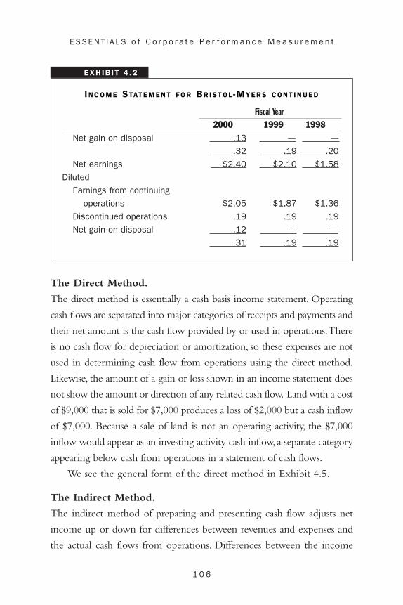
1 0 6
E S S E N T I A L S o f C o r p o r a t e P e r f o r m a n c e M e a s u r e m e n t
EXHIBIT 4 .2
IN C O M E STAT E M E N T F O R BR I S T O L -MY E R S C O N T I N U E D
Fiscal Year
2000 1999 1998Net gain on disposal .13 — —
.32 .19 .20
Net earnings $2.40 $2.10 $1.58
Diluted
Earnings from continuing
operations $2.05 $1.87 $1.36
Discontinued operations .19 .19 .19
Net gain on disposal .12 — —
.31 .19 .19
The Direct Method.
The direct method is essentially a cash basis income statement. Operating
cash flows are separated into major categories of receipts and payments and
their net amount is the cash flow provided by or used in operations.There
is no cash flow for depreciation or amortization, so these expenses are not
used in determining cash flow from operations using the direct method.
Likewise, the amount of a gain or loss shown in an income statement does
not show the amount or direction of any related cash flow. Land with a cost
of $9,000 that is sold for $7,000 produces a loss of $2,000 but a cash inflow
of $7,000. Because a sale of land is not an operating activity, the $7,000
inflow would appear as an investing activity cash inflow, a separate category
appearing below cash from operations in a statement of cash flows.
We see the general form of the direct method in Exhibit 4.5.
The Indirect Method.
The indirect method of preparing and presenting cash flow adjusts net
income up or down for differences between revenues and expenses and
the actual cash flows from operations. Differences between the income

1 0 7
Va r i a t i o n s o f R O I
EXHIBIT 4 .3
Balance Sheet for Bristol-Myers SquibbCompany
Bristol-Myers Squibb Company Consolidated Balance Sheet
December 31,
Dollars in Millions 2000 1999 1998Assets
Current Assets:
Cash and cash equivalents $3,182 $2,720 $2,244
Time deposits and marketable securities 203 237 285
Receivables, net of allowances 3,662 3,272 3,190
Inventories 1,831 2,126 1,873
Prepaid expenses 946 912 1,190
Total Current Assets 9,824 9,267 8,782
Property, plant and equipment 4,548 4,621 4,429
Insurance recoverable 262 468 523
Excess of cost over net tangible assets arising from business acquisitions 1,436 1,502 1,587
Other Assets 1,508 1,256 951
Total Assets $17,578 $17,114 $16,272
Liabilites
Current Liabilities:
Short-term borrowings $162 $432 $482
Accounts payable 1,702 1,657 1,380
Accrued expenses 2,881 2,367 2,302
Product liability 186 287 877
U.S. and foreign income taxes payable 701 794 750
Total Current Liabilities 5,632 5,537 5,791

1 0 8
E S S E N T I A L S o f C o r p o r a t e P e r f o r m a n c e M e a s u r e m e n t
EXHIBIT 4 .3
BA L A N C E SH E E T F O R BR I S T O L -MY E R S C O N T I N U E D
December 31,
Dollars in Millions 2000 1999 1998Other Liabilities 1,430 1,590 1,541
Long-Term debt 1,336 1,342 1,364
Total Liabilities 8,398 8,469 8,696
Stockholders’ Equity
Preferred stock, $2 convertible series: Authorized 10 million shares; issued and outstanding 9,864 in 2000, 10,977 in 1999, and 11,684 in 1998, liquidation value of $50 per share — — —
Common stock, par value of $.10 per share: Authorized 4.5 billion shares; 2,197,900,835 issued in 2000, 2,192,970,504 in 1999, and 2,188,316,808 in 1998 220 219 219
Capital in excess of par value of stock 2,002 1,533 1,075
Other comprehensive income (1,103) (816) (622)
Retained earnings 17,781 15,000 12,540
18,900 15,936 13,212
Less cost of treasury stock—244,365,726common shares in 2000, 212,164,851 in 1999, and 199,550,532 in 1998 9,720 7,291 5,636
Total Stockholders’ Equity 9,180 8,645 7,576
Total Liabilities and Stockholders’ Equity $17,578 $17,114 $16,272

1 0 9
Va r i a t i o n s o f R O I
EXHIBIT 4 .4
Statement of Cash Flows for Bristol-Myers Squibb Company
Bristol-Myers Squibb Company Consolidated Statement of Cash Flows
Year Ended December 31,
In Millions 2000 1999 1998Cash Flow From Operating
Activities:Net earnings $4,711 $4,167 $3,141
Depreciation and amortization 746 678 625
Special charge — — 800
Provision for restructuring/other 542 — 201
Gain from sales of businesses/product divestitures (562) — (201)
Other operating items 10 (79) (1)
Receivables (494) (176) (253)
Inventories 75 (317) (139)
Accounts payable and accrued expenses 256 258 284
Income taxes (54) 477 34
Product liability (173) (726) (715)
Insurance recoverable 100 59 196
Pension contribution (230) — —
Other assets and liabilities (275) (117) (190)
Net Cash Provided by Operating Activities 4,652 4,224 3,782
Cash Flows From Investing Activities:
Proceeds from sales of time deposits and marketable securities 45 51 309
Purchases of time deposits and marketable securities (10) (4) (256)
Additions to fixed assets (589) (709) (788)

1 1 0
E S S E N T I A L S o f C o r p o r a t e P e r f o r m a n c e M e a s u r e m e n t
EXHIBIT 4 .4
STAT E M E N T O F CA S H FL O W S F O R BR I S T O L -MY E R S C O N T I N U E D
Year Ended December 31,
In Millions 2000 1999 1998Proceeds from sales of
businesses/product divestitures 848 134 417
Business acquisitions (including purchase of
trademarks/patents) (196) (266) (93)Other, net (82) 35 65
Net Cash Provided by (Used in) Investing Activities 16 (759) (346)
Cash Flows From Financing Activities:
Short-term borrowings (247) (26) (81)Long-term debt 6 (54) 73Issuances of common stock
under stock plans 352 254 478Purchases of treasury stock (2,338) (1,419) (1,561)Dividends paid (1,930) (1,707) (1,551)
Net Cash Used in Financing Activities (4,157) (2,952) (2,642)
Effect of Exchange Rates on Cash (49) (37) (6)
Increase in Cash and Cash Equivalents 462 476 788
Cash and Cash Equivalents at Beginning of Year 2,720 2,244 1,456
Cash and Cash Equivalents at End of Year $3,182 $2,720 $2,244
The accompanying notes are an Integral part of these financial statements.
statement amounts and the related operating cash flows result in changes
in the current asset and liability accounts because, for the most part, each
of these accounts is linked directly to an operating revenue or expense.
(Inventory and accounts payable, for example, are linked to cost of goods

1 1 1
Va r i a t i o n s o f R O I
Cash Flow Analysis for Bristol-Myers Squibb
2000 1999 1998
Cash return on sales demonstrates the most consistent results.
25.11%25.03%25.54%cash flow
salesCash Return
on Sales�
23.14%28.31%31.04%
estimatedcash flow
total assetsCash ROI �
23.24%24.68%26.46%
cash flowfrom operations
total assetsCash ROI �
I N T H E RE A L WO R L D
sold, accounts receivable to sales revenue.) Cash provided by operations is
thus calculated by (1) adding to net income any changes in current asset or
liability accounts that result in increases in cash from operations,and (2) sub-
tracting from net income any changes that result in decreases. Changes in
the current accounts affect cash flow, as shown in the following:
Add (Subtract) to (from) Net Income
Effect on cash (NI) to Determine Cash Change in Account from operations from OperationsIncrease in
current asset Decrease in cash Subtract from NI
Decrease in
current asset Increase in cash Add to NI
Increase in
current liability Increase in cash Add to NI
Decrease in
current liability Decrease in cash Subtract from NI

1 1 2
E S S E N T I A L S o f C o r p o r a t e P e r f o r m a n c e M e a s u r e m e n t
EXHIBIT 4 .5
Operating Cash Flows Using the Direct Method
Caesar Company Schedule of Operating Cash Flows (Direct Method)
for the year ended December 31, 2001
Cash collected from customers $25,000
Less cash paid for expenses:
For goods sold $10,000
For salaries and wages 7,500
For other operating costs 5,000 22,500
Net cash provided by operating activities $ 2,500
Again, because depreciation and amortization expenses do not affect
cash flows, they are added back to net income. For the same reason, any
losses (or gains) are also adjustments added to (or subtracted from) net
income.
Exhibit 4.6 shows the format for the indirect method of determin-
ing cash flow from operations for ABC Company.The Bristol-Myers’s
Statement of Cash Flows in Exhibit 4.4 uses the indirect method to cal-
culate cash from operations.
Summary
The basic, traditional ROI defines return as net income or income from
operations. Other variations involve defining the return as the gross
margin on sales (gross margin = sales � cost of sales) or as the contri-
bution margin (CM = sales � variable costs) or as the cash flow. The
GMROI is gross margin divided by the average cost of inventory (a
more limited version of investment than total assets). The CMROI is
contribution margin divided by the additional investment in inventory
required to support the sales. The cash ROI divides cash flow from

1 1 3
Va r i a t i o n s o f R O I
EXHIBIT 4 .6
Operating Cash Flows Using the Indirect Method
Caesar Company Schedule of Operating Cash Flows (Indirect Method)
for the year ended December 31, 2001
Net income for 2001 $ 500
Plus:
Depreciation $1,500
Loss on sale of equipment 500
Increase in wages payable 1,000
Decrease in accounts receivable 500 3,500
Less:
Increase in inventory 1,000
Decrease in accounts payable 500 (1,500)
Net cash provided by operating activities $ 2,500
operations by total assets. Each ROI version can be broken down into a
return on sales and a turnover of some type, either inventory turnover
or total asset turnover.As usual, increasing either of the components will
result in an improved ROI.


After read ing th is chapter, you wi l l be ab le to
• Understand how to analyze sales revenues
• Understand the effect of the market on sales revenue per-formance
• Understand the effect of market variance, market share variance, and sales price variance on sales
• Understand the impact of market variance, market share variance, sales price variance, and collection variance onprofit
• Understand price and quantity variances
• Understand the cost behavior of variable and fixed costs
• Understand budget variances
Business centers can often be defined by what their managers are
responsible for controlling. For example, a revenue center manager
controls only sales or some other revenue-generating activity and
is not responsible for either the costs incurred or the investment base
used. Profit center managers are responsible for maximizing profits (and
can control revenues and costs) but not for managing the asset base.An
CHAPTER 5
1 1 5
Analyzing Sales Revenues,Costs, and Profits

1 1 6
E S S E N T I A L S o f C o r p o r a t e P e r f o r m a n c e M e a s u r e m e n t
investment center manager controls either a whole company or a seg-
ment of a company that operates as an autonomous unit, having both
profits and an underlying asset investment base.
Investment, profit, and revenue-center managers contribute to the
profitability of a company and to ROI by increasing revenue produc-
tion as part or all of their duties.Analyzing revenue production involves
more than simply looking at the total dollars of revenue generated. It is
useful to also analyze changes in the market, variations from budget for
total revenues, and any changes from budget in the percentage of cus-
tomer accounts collected. Such changes and variations need to be con-
sidered in the process of variance analysis, which examines differences
in actual results and expected results.
Market Size Variance
Managers are aware that the economy in general can have a great impact
on what they are trying to achieve. If the market for the company’s
products changes, sales revenue will change, independent of the perfor-
mance by a revenue or profit center manager. Any analysis of revenue
generation where a company has a substantial market share (perhaps 10
percent or more) should include a determination of the effect of
changes in market size.
For example, assume the manager of wholesale refrigerator sales in
Chicago is responsible only for the total refrigerator sales revenues gen-
erated.The home office is responsible for all facilities, advertising, and
other costs. In preparing sales forecasts for the year, the manager estab-
lishes a target for Chicago of 50,000 refrigerators at a standard price of
$300 each.The revenue center manager actually sells only 40,000 refrig-
erators during the year, creating a 10,000 unit variance.At the standard
selling price, this creates a $3,000,000 unfavorable (UF) variance from
forecasted sales.

1 1 7
A n a l y z i n g S a l e s R e v e n u e s , C o s t s , a n d P r o f i t s
Forecasted sales 50,000 refrigerators
Actual sales (40,000) refrigerators
Variance 10,000 refrigerators UF
� $300 standard price/refrigerator
$3,000,000 UF
But to analyze the manager’s performance in a meaningful way, we
must first look at the expected market for refrigerators in Chicago and
the market that actually existed.
Forecasted market 500,000 refrigerators
Actual market (450,000) refrigerators
Market variance 50,000 refrigerators UF
From this we see that another way to view the manager’s forecast is
not as 50,000 refrigerators, but as sales of 10 percent of the Chicago
refrigerator market (.10 � 500,000 refrigerators = 50,000 refrigera-
tors).Viewed this way, we see that 5,000 units, or $1,500,000 (5,000
refrigerators � $300 standard price) of the manager’s unfavorable vari-
ance is due to environmental influences the manager could not control,
as follows:
Market Sales @ 10% of MarketForecast 500,000 50,000 refrigerators
Market variance (50,000) UF (5,000) refrigerators UF
Actual market 450,000 refrigerators
Adjusted forecast 45,000 refrigerators
We must evaluate the manager’s performance in relation to the total
revenue available. A decline in the size of the refrigerator market is
beyond the sales manager’s control.

1 1 8
E S S E N T I A L S o f C o r p o r a t e P e r f o r m a n c e M e a s u r e m e n t
Market Share Variance
Once we have corrected for a variance in the size of the market and its
effect on the manager’s forecast, we can determine if the manager
achieved the target or forecasted market share. Here, the manager
expected to sell 45,000 refrigerators (the adjusted target) but sold only
40,000.The manager’s market share has declined by 1.22 percent, result-
ing in an unfavorable variance (UF).
Forecasted market share 50,000/500,000 refrigerators = 10.00%
Less actual market share 40,000/450,000 refrigerators = 8.88%
Market share variance = 1.12% UF
In units and dollars, the market variance and market share variance
are shown as follows.
Market Sales @ 10% of MarketForecast sales 500,000 50,000 refrigerators
Market variance (50,000) (5,000) refrigerators UF
Actual market 450,000 45,000 refrigerators
Actual sales (40,000) refrigerators
Market share variance 5,000 refrigerators UF
� $300 standard price/refrigerator
$1,500,000 UF
In Units At Standard Price
Market Sales @ 10% Sales@ $300 of Market Standard/Unit
Forecast sales 500,000 50,000 $15,000,000
Market variance (50,000) UF (5,000) UF (1,500,000) UF
Actual market 450,000
Adjusted forecast 45,000 13,500,000
Actual quantity sold (40,000) (12,000,000)
Market share variance 5,000 UF $1,500,000 UF
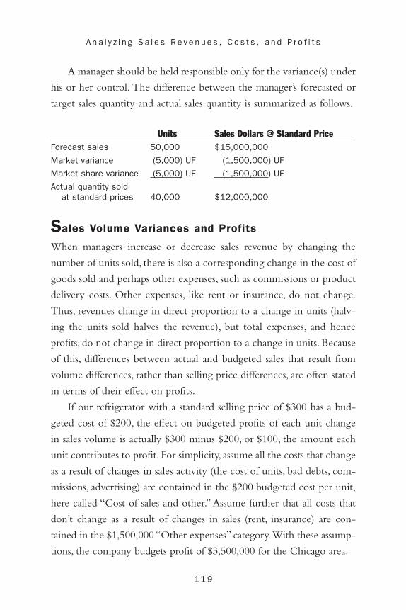
1 1 9
A n a l y z i n g S a l e s R e v e n u e s , C o s t s , a n d P r o f i t s
A manager should be held responsible only for the variance(s) under
his or her control. The difference between the manager’s forecasted or
target sales quantity and actual sales quantity is summarized as follows.
Units Sales Dollars @ Standard PriceForecast sales 50,000 $15,000,000
Market variance (5,000) UF (1,500,000) UF
Market share variance (5,000) UF (1,500,000) UF
Actual quantity sold at standard prices 40,000 $12,000,000
Sales Volume Variances and Profits
When managers increase or decrease sales revenue by changing the
number of units sold, there is also a corresponding change in the cost of
goods sold and perhaps other expenses, such as commissions or product
delivery costs. Other expenses, like rent or insurance, do not change.
Thus, revenues change in direct proportion to a change in units (halv-
ing the units sold halves the revenue), but total expenses, and hence
profits, do not change in direct proportion to a change in units. Because
of this, differences between actual and budgeted sales that result from
volume differences, rather than selling price differences, are often stated
in terms of their effect on profits.
If our refrigerator with a standard selling price of $300 has a bud-
geted cost of $200, the effect on budgeted profits of each unit change
in sales volume is actually $300 minus $200, or $100, the amount each
unit contributes to profit. For simplicity, assume all the costs that change
as a result of changes in sales activity (the cost of units, bad debts, com-
missions, advertising) are contained in the $200 budgeted cost per unit,
here called “Cost of sales and other.” Assume further that all costs that
don’t change as a result of changes in sales (rent, insurance) are con-
tained in the $1,500,000 “Other expenses” category.With these assump-
tions, the company budgets profit of $3,500,000 for the Chicago area.

1 2 0
E S S E N T I A L S o f C o r p o r a t e P e r f o r m a n c e M e a s u r e m e n t
Budgeted Income for Chicago at Budgeted QuantitySales at standard cost (50,000 � $300) $15,000,000
Cost of sales and other at budgeted cost (50,000 � $200) 10,000,000
Budgeted gross margin 5,000,000
Other expenses not changing with sales 1,500,000
Budgeted net income $3,500,000
If we change the budgeted sales quantity to the actual sales quantity
of 40,000 units, and keep the standard selling price at $300, the bud-
geted cost per unit at $200, and “Other expenses” at $1,500,000, we find
income decreases by $1,000,000. (This is what we expect because we
know that each unit sold is budgeted to contribute $100 to profit and
50,000 � 40,000 = 10,000 units � $100 = $1,000,000.)
Budgeted Income for Chicago at Actual QuantitySales at standard cost (40,000 � $300) $12,000,000
Cost of sales and other at budgeted cost (40,000 � $200) 8,000,000
Budgeted gross margin 4,000,000
Other expenses not changing with sales 1,500,000
Budgeted net income at actual quantity $ 2,500,000
Working from these income statements, our analysis of volume
changes due to market and market share variances explain the change
in profit, as follows.
Units Profit Total Profit per Unit in Dollars
Forecast profit $3,500,000
Market variance (5,000) UF � $100 (500,000) UF
Market share variance (5,000) UF � $100 (500,000) UF
Profit after market variances $2,500,000

1 2 1
A n a l y z i n g S a l e s R e v e n u e s , C o s t s , a n d P r o f i t s
Sales Price Variances
Managers can try to improve the bottom line by increasing market share
(as just discussed) or by increasing selling prices.When there is a change
in the selling price of a company’s products, the increase or decrease
goes directly to the bottom line because there is no accompanying
change in cost. If the manager in our example actually sold 40,000
refrigerators at $315 (rather than at the forecasted price of $300), the
$15 increase in selling price per unit results in a $15 per unit increase in
profit.The variance due to the change in selling price is $600,000 favor-
able (F), as follows.
40,000 units � $15/unit increase in selling price = $600,000 F
At an actual selling price of $315/unit and an actual volume of
40,000 units, total sales revenues are $12,600,000 (40,000 units �
$315), and the difference between the manager’s forecasted sales and
actual sales performance is now summarized as follows. Notice that each
of the variances is shown separately to highlight how it alone affects
sales, and actual sales contains the effect of all three variances.
Standard PriceUnits per Unit Sales Dollars
Forecast sales 50,000 � $300 $15,000,000
Sales volume variances:
Market variance (5,000) UF � 300 (1,500,000) UF
Market share variance (5,000) UF � 300 (1,500,000) UF
Sales price variance NA 600,000) F
Actual sales 40,000 $12,600,000
When the actual selling price is $315/unit, the effect on budgeted
profits of the market, market share, and sales price variances is shown as
follows.

1 2 2
E S S E N T I A L S o f C o r p o r a t e P e r f o r m a n c e M e a s u r e m e n t
Standard Profit Profit Units per Unit in Dollars
Forecast profit NA $3,500,000
Sales volume variances:
Market variance (5,000) UF � $100 (500,000) UF
Market share variance (5,000) UF � 100 (500,000) UF
Sales price variance NA 600,000) F
Actual profit $3,100,000
Sales Collection Variance
Chapter 4 discusses Cash ROI and points out that earnings must be
accompanied by cash flows for investors to believe earnings are of high
quality. Cash flows from sales are often determined by the company’s
ability to collect credit sales. If the company fails to screen customers
properly or to anticipate economic downturns, sales result in uncol-
lectible accounts expense rather than in cash inflows.
Thus, it is useful to reconcile budgeted cash collections from sales
to actual cash collected from sales. If collection is a problem, determin-
ing and isolating a sales collection variance demonstrates that collections
are as important as sales volume or selling price.
Assume the company in our example sells on credit and budgets
uncollectible sales at 6 percent of total sales. Due to a change in credit
policy, the company actually has uncollectible sales of 10 percent.
Uncollectible sales are four percentage points (10% � 6%) higher than
forecasted, and the sales collection variance is 4 percent of $12,600,000,
or $504,000 UF.
An analysis of the difference between actual and budgeted perfor-
mance that includes a consideration of the cash collection variance
follows.

1 2 3
A n a l y z i n g S a l e s R e v e n u e s , C o s t s , a n d P r o f i t s
Units Sales DollarsForecast sales 50,000 $15,000,000
Sales volume variances:
Market variance (5,000) UF (1,500,000) UF
Market share variance (5,000) UF (1,500,000) UF
Sales price variance NA 600,000) F
Actual sales 40,000 $12,600,000
Less:
Budgeted uncollectible sales (6%) (756,000)
Budgeted cash collections from sales $11,844,000
Collection variance (4%) (504,000) UF
Actual cash collected from sales (90%) $11,340,000
The company’s forecasted profit includes the budgeted uncollectible
accounts expense. The collection variance is in substance a variance in
uncollectible accounts expense. Changes in uncollectible accounts
expense (labeled “Collection variance”) are included in a reconciliation
of budgeted and actual profits, as follows.
Units Profit in DollarsForecast profit $3,500,000
Sales volume variances:
Market variance (5,000) UF (500,000) UF
Market share variance (5,000) UF (500,000) UF
Sales price variance 600,000) F
Actual profit before collection variance $3,100,000
Collection variance (504,000) UF
Actual profit $2,596,000
Summary Analysis
The manager in our example forecast sales of 10 percent of the Chicago
refrigerator market, to consist of 50,000 refrigerators sold for an average

1 2 4
E S S E N T I A L S o f C o r p o r a t e P e r f o r m a n c e M e a s u r e m e n t
(standard) price of $300 each, or total sales of $15,000,000.The manager’s
actual profit for the year is $2,596,000 on sales of $12,600,000. Profits are
$904,000 less than target, and sales are off by $2,400,000 ($1,500,000 +
$1,500,000 � $600,000, or market variance + market share variance �
sales price variance).
The manager’s performance is analyzed as follows:The Chicago mar-
ket was 10 percent less than the forecast, and the manager lost 10 percent
of the company’s predicted unit market share. The combined effect of
these losses reduced sales by $3,000,000 and profits by $1,000,000. In
response to slow profit growth, the manager increased selling price to
average $315 per unit for the year and loosened credit terms. Some of
the lost sales dollars were recovered as a result of the increased price.
Profits increased by $600,000 as a result of the price change, but fell
$504,000 because of higher uncollectibles resulting from the new credit
policies.
There may also be variances from the budgeted $200 per unit or the
budgeted $1,500,000 in other expenses, but the Chicago manager is
responsible only for sales revenues. Some other manager is responsible
for any other variances.
Income Performance for Chicago (With budgeted cost of sales and other expenses but actual quantity, price, and collection rate controllable by the Chicago manager)Sales (40,000 � $315) $12,600,000
Cost of sales and other at budgeted cost (40,000 � $200) 8,000,000
Budgeted gross margin 4,600,000
Additional uncollectible accounts expense* 504,000
Other expenses not changing with sales (budgeted) 1,500,000
Net income $ 2,596,000*Because of our beginning assumptions, the budgeted 6 percent uncollectible accountsexpense must be included in the $200/unit “Cost of sales and other.” Only the 4 percentadditional amount is shown as additional uncollectible accounts expense.

1 2 5
A n a l y z i n g S a l e s R e v e n u e s , C o s t s , a n d P r o f i t s
Variable Costs Variance
So far we have looked at techniques used to analyze variances in return
caused by revenues that vary from a targeted or budgeted level. The
remainder of the chapter discusses variances in return resulting from
costs that are different from budget.The variances in this chapter are used
as the starting point in detailed analysis of variations in profit and ROI.
Variable costs are expected to vary in total in direct proportion with
activity.Examples of items that are generally variable costs include the cost
of energy, raw materials, supplies, maintenance, and assembly-line labor.
Exhibit 5.1 shows the graph of a typical variable cost.
Variable Cost Standards
Variable cost budgets for departments or projects are generally prepared
by first estimating the cost of each individual component activity of the
department or project. For example, budgets for the cost of the payroll
department may begin with budgets for such items as the cost of autho-
rizing and printing one check, or the marginal (or additional) cost of
typing and mailing one letter. Total budgeted payroll department costs,
then, are determined as the total of 52 weekly payrolls of 200 checks at
$150 per check, plus 50,000 letters per year at a budgeted cost per let-
ter of $4, plus budgeted amounts for the costs of other activities.
The cost of each activity for which costs are budgeted separately is
often called a standard cost. Thus, we speak of the standard cost of print-
ing a weekly payroll check, or the standard cost per letter typed and
mailed.Whatever the activity, its total standard cost is determined from
the standard or budgeted quantity of an input allowed for a unit and the
standard or budgeted cost of the input.
standard quantityof inputs
�standard price
of inputs�
standard costof output
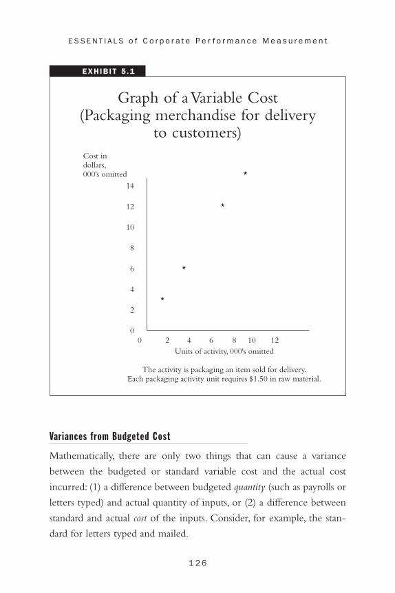
1 2 6
E S S E N T I A L S o f C o r p o r a t e P e r f o r m a n c e M e a s u r e m e n t
Variances from Budgeted Cost
Mathematically, there are only two things that can cause a variance
between the budgeted or standard variable cost and the actual cost
incurred: (1) a difference between budgeted quantity (such as payrolls or
letters typed) and actual quantity of inputs, or (2) a difference between
standard and actual cost of the inputs. Consider, for example, the stan-
dard for letters typed and mailed.
Graph of a Variable Cost(Packaging merchandise for delivery
to customers)
EXHIBIT 5 .1
14
12
10
8
6
4
2
00 2 4 6 8 10 12
Units of activity, 000's omitted
The activity is packaging an item sold for delivery.Each packaging activity unit requires $1.50 in raw material.
Cost indollars,000's omitted *
*
*
*

1 2 7
A n a l y z i n g S a l e s R e v e n u e s , C o s t s , a n d P r o f i t s
The actual, total cost is different from budget if a different quantity
of letters are typed, say 55,000 letters instead of the 50,000 budgeted.
The quantity variance is $20,000 unfavorable ($220,000 � $200,000).
An alternate way to calculate a quantity variance is
Actual results also differ from budget if the activity actually costs
more or less than the cost allowed by the standard.Assume the admin-
istration department not only types 5,000 more letters than expected,
but also pays $5 per letter typed, rather than the $4 price budgeted as
standard.
The price variance is $55,000 unfavorable ($275,000 � $220,000). An
alternate way to calculate a price variance is as follows.
Actual Quantityof Inputs
55,000 letters
�
�
Change in Priceof Inputs
$1>letter unfavorable
�
�
Price Variance
$55,000 unfavorable
Actual Quantityof Inputs
55,000 letterstyped
�
�
Actual Priceof Inputs
$5>letter
�
�
Actual Costof Actual Output
$275,000
Change in Quantityof Inputs
5,000 additionalletters
�
�
Standard Priceof Inputs
$4>letter
�
�
QuantityVariance
$20,000unfavorable
Actual Quantityof Inputs
55,000 letters
�
�
Standard Priceof Inputs
$4>letter
�
�
Standard Costof Actual Output
$220,000
Budgeted Quantityof Inputs
50,000 letters
�
�
Standard Priceof Inputs
$4>letter
�
�
Budgeted Costof Output
$200,000
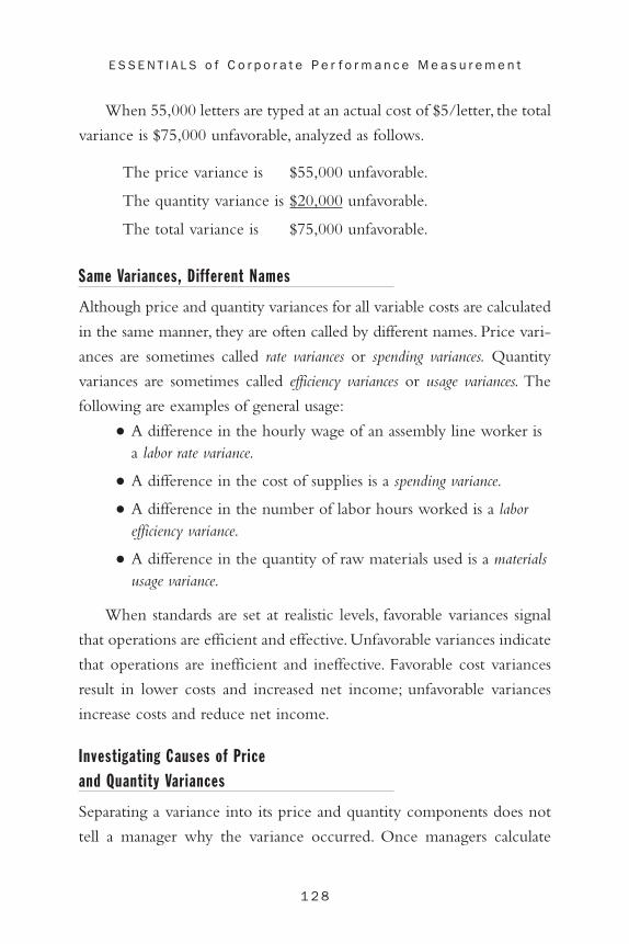
1 2 8
E S S E N T I A L S o f C o r p o r a t e P e r f o r m a n c e M e a s u r e m e n t
When 55,000 letters are typed at an actual cost of $5/letter, the total
variance is $75,000 unfavorable, analyzed as follows.
The price variance is $55,000 unfavorable.
The quantity variance is $20,000 unfavorable.
The total variance is $75,000 unfavorable.
Same Variances, Different Names
Although price and quantity variances for all variable costs are calculated
in the same manner, they are often called by different names. Price vari-
ances are sometimes called rate variances or spending variances. Quantity
variances are sometimes called efficiency variances or usage variances. The
following are examples of general usage:
• A difference in the hourly wage of an assembly line worker isa labor rate variance.
• A difference in the cost of supplies is a spending variance.
• A difference in the number of labor hours worked is a laborefficiency variance.
• A difference in the quantity of raw materials used is a materialsusage variance.
When standards are set at realistic levels, favorable variances signal
that operations are efficient and effective. Unfavorable variances indicate
that operations are inefficient and ineffective. Favorable cost variances
result in lower costs and increased net income; unfavorable variances
increase costs and reduce net income.
Investigating Causes of Price
and Quantity Variances
Separating a variance into its price and quantity components does not
tell a manager why the variance occurred. Once managers calculate
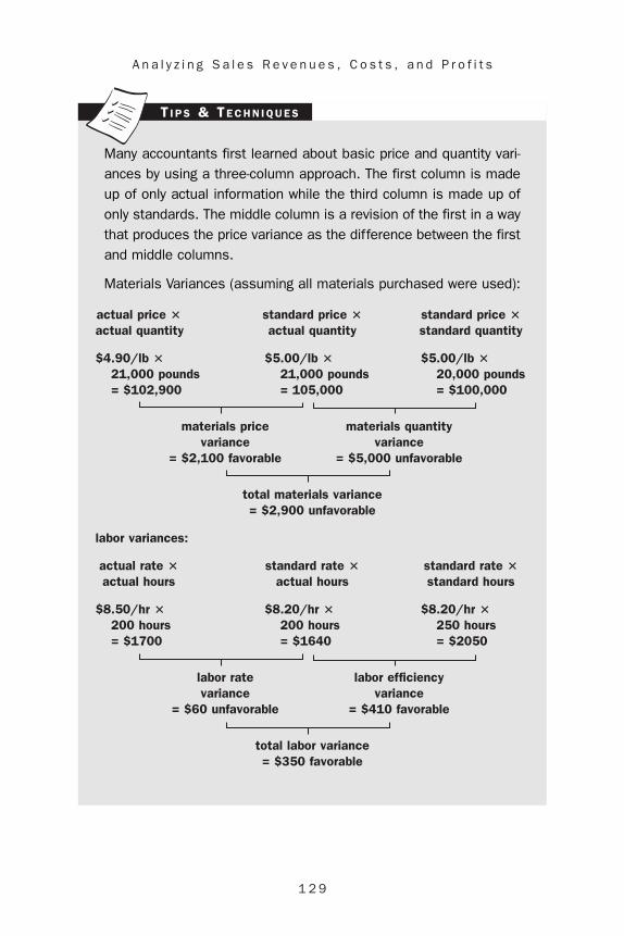
1 2 9
A n a l y z i n g S a l e s R e v e n u e s , C o s t s , a n d P r o f i t s
Many accountants first learned about basic price and quantity vari-ances by using a three-column approach. The first column is madeup of only actual information while the third column is made up ofonly standards. The middle column is a revision of the first in a waythat produces the price variance as the difference between the firstand middle columns.
Materials Variances (assuming all materials purchased were used):
actual price � standard price � standard price �actual quantity actual quantity standard quantity
$4.90/lb � $5.00/lb � $5.00/lb �21,000 pounds 21,000 pounds 20,000 pounds = $102,900 = 105,000 = $100,000
materials price materials quantity variance variance
= $2,100 favorable = $5,000 unfavorable
total materials variance= $2,900 unfavorable
labor variances:
actual rate � standard rate � standard rate �actual hours actual hours standard hours
$8.50/hr � $8.20/hr � $8.20/hr �200 hours 200 hours 250 hours = $1700 = $1640 = $2050
labor rate labor efficiency variance variance
= $60 unfavorable = $410 favorable
total labor variance= $350 favorable
T I P S & TE C H N I Q U E S
1 3 0
E S S E N T I A L S o f C o r p o r a t e P e r f o r m a n c e M e a s u r e m e n t
price and quantity variances, they must investigate to see why the vari-
ances occurred. In our example, the actual cost per letter might increase
because of a change in the cost of paper or postage. It might simply be
that the $4 standard is inaccurate or out of date.The number of letters
might increase because the number of employees, customers, or vendors
with whom the company corresponds increased. Or perhaps manage-
ment decided to improve relations by increasing its communications
with one of these groups.
Alternately, an increase in computerization or the use of form letters
might reduce the cost per letter. Increased use of electronic mail (e-mail)
might reduce the number of letters. Exhibit 5.2 lists a few of the causes
a manager might find for variances in correspondence cost.
Sometimes a variance in one department is caused by poor work
done in another department. If, for instance, an employee in the pur-
chasing department buys low-quality envelopes at a price below the
purchasing standard, that will generate a favorable price variance in the
purchasing department. But if the envelopes have a poor-quality glue,
they might stick together or fail to seal. Difficulty using the cheap, low-
quality envelopes might increase the cost to process each letter.
Fixed Cost Variances
Fixed costs are costs that do not vary in total with changes in activity.A
fixed cost remains constant or fixed in total, despite changes in operat-
ing activity. Examples of fixed costs include the cost of fire insurance or
property taxes on a building, the lease payment for a computer or car,
and the monthly compensation of all salaried workers. Exhibit 5.3
shows the graph of a typical fixed cost.
It is relatively easy to estimate the amount of variable cost per unit of
activity: simply increase activity 10 (or 100 or 1,000) units, and total vari-
able costs increase by 10 (or 100 or 1,000) times the variable cost per

1 3 1
A n a l y z i n g S a l e s R e v e n u e s , C o s t s , a n d P r o f i t s
EXHIBIT 5 .2
Payroll Department:Reasons for Cost Variances Processing Correspondence
Price variances may result from:
Changes in postage
Changes in the cost of stationery or envelopes
Changes in the specified quality of stationery or envelopes
Changes in the wages of typists or other workers involved
Changes in the level of skill specified in typist or other job
descriptions
Turnover in the department
Hiring part-time help
Changes in the level of computerization
Aging of equipment
Quantity variances may result from:
Changes in the number of employees or others receiving
correspondence
Increased use of E-mail
Changes in policy
Changes in the use of bulletin boards
Changes in the company environment requiring communica-
tion to workers
New management styles

1 3 2
E S S E N T I A L S o f C o r p o r a t e P e r f o r m a n c e M e a s u r e m e n t
Employee Participation in Variance Analysis
As mentioned in the text, managers must investigate to see whyvariances occurred. Employees may be in a position to help in thisinvestigation as it relates to efficiency variances, since employeesare the ones using the materials to produce a product and spend-ing the labor time on the product. Furthermore, managers often findthat when they involve employees in decision making, moraleimproves and operations become more effective and efficient.According to “America’s Elite Factories” in Fortune magazine, theKenworth Truck Plant in Renton, Washington, has experienced thisvery situation. Employees of Kenworth are encouraged to make sug-gestions on how to improve efficiency, and the company readilyapproves good suggestions, recently rearranging placement of partsto economize on employee time spent obtaining parts during pro-duction. In the same article, Aeroquip Group in Van Wert, Ohio, ispraised for building—and rebuilding—production cells in its questfor greater efficiency and for attaining 95 percent employee partici-pation in its “improvement teams.” This participation has drasticallycut cycle times. In such environments as these, variances would notbe insurmountable obstacles.
Gene Bylinsky. “America’s Elite Factories,” Fortune (August 14, 2000). http://www.fortune.com/indext.jhtml?channel=print_article.jhtml%doc_id=00000743.
I N T H E RE A L WO R L D
unit. For example, if we increase the number of letters typed by 10, total
cost increases by $50 (10 � $5). Dividing the $50 increase by the 10-let-
ter increase in activity gives us the variable cost of $5/letter.The cost per
unit of a variable cost does not change in response to changes in activity.
It is not easy to determine a per-unit amount for fixed costs because
total fixed costs do not change when activity is changed. The payroll
department manager’s salary, perhaps $75,000, is the same at 50,000 let-

1 3 3
A n a l y z i n g S a l e s R e v e n u e s , C o s t s , a n d P r o f i t s
Graph of a Fixed Cost(Leased equipment)
EXHIBIT 5 .3
$10,000 total cost
$14
12
10
8
6
4
2
0
0 2 4 6 8 10 12 14Units produced, 000's omitted
The equipment lease is $10,000 annually.
Cost indollars,000's omitted
ters as at 55,000. In fact, the fixed cost per unit of activity changes each
time total activity changes, as illustrated below and in Exhibit 5.4.
(These illustrations include the unrealistic assumption that the entire
salary relates to letters processed.)
$75,000 salary divided by 50,000 letters = $1.50/letter.
$75,000 salary divided by 55,000 letters = $1.36/letter.
$75,000 salary divided by 65,000 letters = $1.15/letter.
$75,000 salary divided by 75,000 letters = $1.00/letter.

1 3 4
E S S E N T I A L S o f C o r p o r a t e P e r f o r m a n c e M e a s u r e m e n t
Graph of Manager’s Salary
EXHIBIT 5 .4
$1.50/unit
$1.36/unit
$1.15/unit
$1.00/unit
50,0000
75,000
Cost indollars
Letters processed
The manager's salary is a $75,000 fixed cost.
55,000 65,000 75,000
Because fixed costs are not directly affected by specific activities as
variable costs are, fixed costs must be assigned or allocated to units of
activity in an arbitrary way. If, at the beginning of the year, the budget
for the payroll department included a $75,000 salary for the department
manager, the cost per letter or check can be determined only arbitrar-
ily. Since the manager’s salary pays for managing not only correspon-
dence, but also preparing checks and perhaps performing other
activities, we must first divide the salary among those areas. How much

1 3 5
A n a l y z i n g S a l e s R e v e n u e s , C o s t s , a n d P r o f i t s
of the manager’s salary should be allocated to letters? To checks? To
other activities?
Allocating Fixed Costs
Let’s say a consultant watches the manager and determines that 20 per-
cent of the manager’s time is devoted to supporting letter writing and
processing, 30 percent to weekly payrolls, and 50 percent to various other
activities (perhaps the preparation of checks for salaried personnel).
Using the previously budgeted activity levels of 50,000 letters and 100
checks each week (or 5,200 per year), per-unit amounts are as follows:
Letter writing and processing:
Payroll check preparation:
(Other activities are assigned the remaining $37,500 [$75,000 � .50].)
The salary/unit amounts we calculated are affected by changes in
volume.What if the company started a second shift, adding another 100
workers—would the cost still be $4.33/check written? Probably not.
The manager’s salary might well stay the same, regardless. Likewise, the
proportion of the manager’s effort (however measured) necessary to
process the weekly payroll might increase only a small amount, if at all.
(After all, the manager is responsible for managing the check-writing
process, not creating the checks.) In all likelihood, the manager’s salary per
check at 200 checks per week would simply be half what it was at 100.
$75,000 � .30 � $22,500 divided by 5,200 checks
� $4.33 salary>check
$75,000 � .20 � $15,000 divided by 50,000 letters
� $0.30 salary>letter
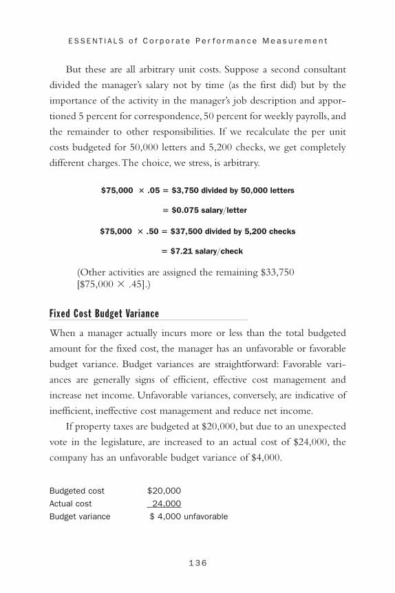
1 3 6
E S S E N T I A L S o f C o r p o r a t e P e r f o r m a n c e M e a s u r e m e n t
But these are all arbitrary unit costs. Suppose a second consultant
divided the manager’s salary not by time (as the first did) but by the
importance of the activity in the manager’s job description and appor-
tioned 5 percent for correspondence, 50 percent for weekly payrolls, and
the remainder to other responsibilities. If we recalculate the per unit
costs budgeted for 50,000 letters and 5,200 checks, we get completely
different charges.The choice, we stress, is arbitrary.
(Other activities are assigned the remaining $33,750 [$75,000 � .45].)
Fixed Cost Budget Variance
When a manager actually incurs more or less than the total budgeted
amount for the fixed cost, the manager has an unfavorable or favorable
budget variance. Budget variances are straightforward: Favorable vari-
ances are generally signs of efficient, effective cost management and
increase net income. Unfavorable variances, conversely, are indicative of
inefficient, ineffective cost management and reduce net income.
If property taxes are budgeted at $20,000, but due to an unexpected
vote in the legislature, are increased to an actual cost of $24,000, the
company has an unfavorable budget variance of $4,000.
Budgeted cost $20,000
Actual cost 24,000
Budget variance $ 4,000 unfavorable
$75,000 � .50 � $37,500 divided by 5,200 checks
� $7.21 salary>check
$75,000 � .05 � $3,750 divided by 50,000 letters
� $0.075 salary>letter

1 3 7
A n a l y z i n g S a l e s R e v e n u e s , C o s t s , a n d P r o f i t s
Managers must investigate to find and, if possible, remedy the causes
of unfavorable fixed cost variances. In this case, an increase in property
taxes is beyond management’s control.
Setting Standards
Managers sometimes set standards based on results obtained in the past,
perhaps adjusted for inflation or a change in operating methods. But,
using historical results to set standards tends to perpetuate the ineffi-
ciencies of the past by incorporating them in expectations about the
future.
Time-and-motion studies and other engineering methods are fre-
quently used to set labor standards. Engineers may also set equipment
maintenance standards or establish specifications for materials in a man-
ufacturing operation. Such approaches do not use historical data but
may set standards using unattainable engineering ideals.
Perhaps the best method is to use the judgment of the managers
who must meet the standards in a participative standard-setting process.
This may create standards that are more realistic than idealistic. Managers
who help set standards are generally more committed to meeting them.
Summary
When managers are evaluated according to what they are responsible
for controlling, there must be a way to measure when they have not met
expectations. And there must be a way to identify why their perfor-
mance did not meet expectations. A number of variances have been
developed to aid in this evaluation process.The market size variance will
help identify when revenues and profits have been affected by a change
in the market (a factor probably outside the manager’s control). The
manager’s performance can be assessed by analyzing such variances as

1 3 8
E S S E N T I A L S o f C o r p o r a t e P e r f o r m a n c e M e a s u r e m e n t
the market share variance (since a manager can certainly strive to obtain
a bigger share of the market), the sales price, and sales collections vari-
ances (since the manager can affect pricing and cash collection policies).
Managers not only control circumstances related to revenues and
cash collections, they also may control costs. Price and quantity vari-
ances are useful in evaluating management’s control over raw materials
or labor or fixed costs. Management can identify where a variance
occurs and then investigate why it occurred.
CHAPTER 6
1 3 9
ROI and InvestmentCenters
After read ing th is chapter, you wi l l be ab le to
• Understand the characteristics of an investment center
• Understand the advantages and disadvantages of decentral-ized management versus centralized management
• Understand alternative means of setting transfer prices
Calling a segment of the company an investment center seems like a
great idea. Managers are often eager to designate segments of the
company as investment centers and use ROI for performance
evaluation and control. But before top managers designate an opera-
tion as an investment center, they should be sure it has four important
characteristics:
1. Autonomous operations
2. Free access to vendors and customers
3. Separate revenues and costs
4. Management design
Autonomous Operations
Managers must be certain that a segment is an independent operating
unit before they can gain the benefits of an investment center.The man-
ager of the segment must control most operating decisions, subject only

1 4 0
E S S E N T I A L S o f C o r p o r a t e P e r f o r m a n c e M e a s u r e m e n t
EXHIBIT 6 .1
Geographic Decentralization withProduction in Each Location
ChicagoFactory 1
New YorkFactory 2
New OrleansFactory 3
AtlantaFactory 4
NashvilleHome Office
Factory 5
to broad policy guidance from top management.The segment manager
must control—completely or in large measure—investment in capital
assets, their maintenance schedules, production volumes, product mix,
and prices.
Manufacturing operations, retail and wholesale outlets, and cus-
tomer service and repair centers are examples of segments where this
level of independent operating control is possible. Segments such as
advertising departments, internal maintenance departments, and person-
nel usually cannot be independent in the same way and, therefore, can-
not be investment centers evaluated by ROI.
Autonomous operating units are common to decentralized compa-
nies, although complete decentralization is not a prerequisite for inde-
pendent segments. The intuitive image of a decentralized company is
one with geographically dispersed branches (as in Exhibit 6.1), but
decentralized management does not require physically separate operat-

1 4 1
R O I a n d I n v e s t m e n t C e n t e r s
EXHIBIT 6 .2
Decentralized Management withAuthority in Each Department
Personnel
Maintenance
Administration
Production
Shipping
Receiving
NashvilleHome Office
Factory 5
ing segments. Decentralized management delegates decision-making
authority to lower levels of operating management, as shown in Exhibit
6.2.These managers are often more responsive than headquarters to the
conditions in their operating units.
In a company using a centralized management approach, top man-
agement retains direct control of operations; lower levels of manage-
ment do not make major decisions.The advantages and disadvantages
of decentralized and centralized management are in Exhibits 6.3 and
6.4.
Free Access to Vendors and Customers
An investment center manager must have free access to suppliers and
markets, both inside and outside the company. The manager must be
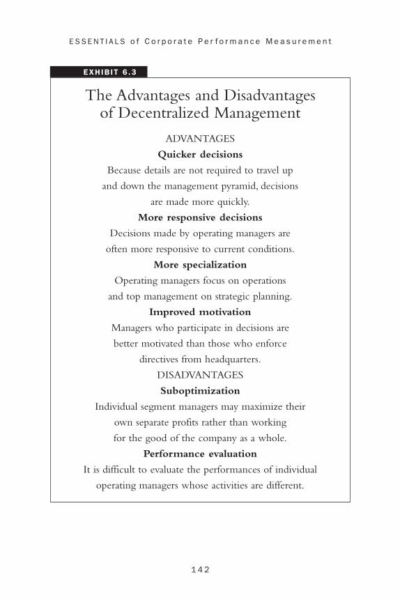
1 4 2
E S S E N T I A L S o f C o r p o r a t e P e r f o r m a n c e M e a s u r e m e n t
EXHIBIT 6 .3
The Advantages and Disadvantages of Decentralized Management
ADVANTAGES
Quicker decisions
Because details are not required to travel up
and down the management pyramid, decisions
are made more quickly.
More responsive decisions
Decisions made by operating managers are
often more responsive to current conditions.
More specialization
Operating managers focus on operations
and top management on strategic planning.
Improved motivation
Managers who participate in decisions are
better motivated than those who enforce
directives from headquarters.
DISADVANTAGES
Suboptimization
Individual segment managers may maximize their
own separate profits rather than working
for the good of the company as a whole.
Performance evaluation
It is difficult to evaluate the performances of individual
operating managers whose activities are different.

1 4 3
R O I a n d I n v e s t m e n t C e n t e r s
EXHIBIT 6 .4
The Advantages and Disadvantages of Centralized Management
ADVANTAGES
Better control
Centralized management can easily
focus on a clear corporate goal.
Economies of scale
One large operation is often more
efficient than several smaller, decentralized operations.
DISADVANTAGES
Increased complexity
Large, centrally controlled entities that combine several
different operations are often complex and hard
to manage effectively.
Diseconomies of scale
Large operations are often more difficult to control
and keep efficient than are several smaller,
decentralized operations.
Span of control
The larger an operation grows, the more
difficult it is to control everything from the top.
able to barter for the lowest cost when buying and must demand the
best price when selling. For example, the manager of a segment that uses
copper wire must be free to buy from the company’s copper-wire pro-
duction segment, or, if price, quality, or service are better, from outside
the company.The same conditions must apply to the copper production

1 4 4
E S S E N T I A L S o f C o r p o r a t e P e r f o r m a n c e M e a s u r e m e n t
segment (if it is to be an investment center).That segment must be able
to sell its wire outside the company if a better price is offered.
Restricting segment managers to buying or selling to particular
units within the company prevents them from being free to improve
their return, a situation that can reduce morale and incentive.With free
access to suppliers and markets, each autonomous segment will find the
most efficient, effective, and economical methods for purchasing, pro-
duction, and marketing.
When segments are free to purchase both inside and outside the
company, segments that do a poor job competing with markets or sup-
pliers outside the company will not survive. If the copper-wire opera-
tion cannot successfully produce copper wire and sell it to the
downstream segment in competition with outside producers, the com-
pany as a whole is better off discontinuing the operation.
Separate Revenues and Costs
An investment center must be able to separate its costs and revenues
from the rest of the company.Without this ability the segment cannot
determine a profit return. If a segment sells its production to another
segment in the same company, there might be a degree of arbitrariness
to the selling or transfer price established between the two operations.
If the production is specialized, perhaps tailormade for use in the
downstream division’s operation, there may be no realistic way to set
an objective price.This problem is discussed later in the chapter.
Management Design
Management must consider the objectives of a segment and decide that
the segment will be most focused on its objectives if it operates as an
investment center. For example, assume a molding operation receives its
molding compounds from an upstream department, molds the com-
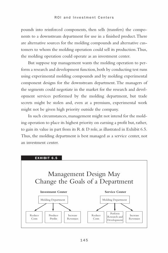
1 4 5
R O I a n d I n v e s t m e n t C e n t e r s
EXHIBIT 6 .5
Management Design May Change the Goals of a Department
ReduceCosts
ProduceProfits
IncreaseRevenues
Molding Department
Investment Center
ReduceCosts
PerformResearch andDevelopment
IncreaseRevenues
Molding Department
Service Center
pounds into reinforced components, then sells (transfers) the compo-
nents to a downstream department for use in a finished product.There
are alternative sources for the molding compounds and alternative cus-
tomers to whom the molding operation could sell its production.Thus,
the molding operation could operate as an investment center.
But suppose top management wants the molding operation to per-
form a research and development function, both by conducting test runs
using experimental molding compounds and by molding experimental
component designs for the downstream department. The managers of
the segments could negotiate in the market for the research and devel-
opment services performed by the molding department, but trade
secrets might be stolen and, even at a premium, experimental work
might not be given high priority outside the company.
In such circumstances, management might not intend for the mold-
ing operation to place its highest priority on earning a profit but, rather,
to gain its value in part from its R & D role, as illustrated in Exhibit 6.5.
Thus, the molding department is best managed as a service center, not
an investment center.

1 4 6
E S S E N T I A L S o f C o r p o r a t e P e r f o r m a n c e M e a s u r e m e n t
Other segments might completely lose their usefulness operating as
an investment center. The company might, for instance, employ high-
powered experts in its market research department who are capable of
operating as an autonomous consulting group, offering services to
clients in and out of the company. But to undertake market research in
this way defeats the purpose of the department.The operating objective
of the market research group must be to improve the market position of
the company, not create a segment profit.The same is true of the legal
department, public relations, and other service departments.
ROI and Transfers between Segments
Investment centers must have separable revenues and costs.This is not a
problem when there are alternative vendors and customers outside the
company. In such cases, segments buy, sell, and transfer products from one
to the other at competitive market prices.As a result, companies invest in
activities that promise to generate the best returns.Conversely, if a segment
grows inefficient and cannot operate in competition with producers out-
side the company, it will find no customers for its output inside or outside
the company.Then it cannot continue. Investments in unprofitable oper-
ations are moved to profitable operations. If a segment competes success-
fully with suppliers outside the company, it finds customers for its output
and its profitability justifies requests for additional capital or other support.
When there is no alternative vendor or customer and no true mar-
ket reference price, problems can arise. In this situation, managers often
create pseudomarket transfer prices based on several different general
models. All these attempts to contrive an artificial measure to replace
market price have the potential to cause problems and reduce ROI.
The six most common problems associated with transfer prices
other than a competitively set market price are as follows:

1 4 7
R O I a n d I n v e s t m e n t C e n t e r s
1. Misdirected capital investments made based on artificial returns
2. Misdirected operating funds because budgets are based on artifi-cial cost and revenue figures
3. Bonuses and other performance rewards based on assessmentsusing negotiated or mandated results, rather than real costs andrevenues
4. Erroneous actions resulting from evaluations of problems andopportunities distorted by ignorance of true revenues and costs,including opportunity costs
5. Inappropriate responses to changes in markets and competitorsdue to costs and revenues that do not reflect these processes
6. Poor morale among segment managers, resulting from percep-tions of differential treatment
Transfer Prices
Transfer prices used in place of actual market prices established in com-
petition with producers outside the company vary greatly in their use-
fulness and their potential for harm.There are four methods of setting
transfer prices that are in wide use.
Published Market Prices
Many companies that do not allow segments to buy or sell outside the
company use published market prices to transfer intermediate products
between segments. Published market prices are also adapted for use as
transfer prices when the actual intermediate product is a different (per-
haps custom-made) type, grade, or quality than the products whose
prices are published.
Often, published prices of intermediate products are for different
quantities of product, in a different location, than the product trans-
ferred. Published prices are usually spot prices, rather than long-term

1 4 8
E S S E N T I A L S o f C o r p o r a t e P e r f o r m a n c e M e a s u r e m e n t
Transfer Pricing
Transfer pricing can be a thorny issue, as shown by the followinganecdote from “Sandy Weill’s Monster” in Fortune.
In an institution that promotes cross-selling, for example,there is always the question of how the financial spoils aredivided up between the two divisions—a matter that goesunder the name transfer pricing. For example, suppose thata Salomon Smith Barney financial consultant sells a mutualfund “manufactured” by Citi’s investment management divi-sion. What’s the price that the IM division receives? Theanswer, since it determines profit, is extremely important toexecutives getting paid (and paying their people) accordingto what their own bottom line looks like. One former Citiexecutive says that difficult questions like these havesometimes aggravated business heads to the point of their“barely speaking to each other.”
Asked about transfer pricing pains at Citi, Weill saystestily that he wishes people “would think about doing thebusiness first, and worry about who gets the credit sec-ond.” But, trying to mediate, he also has his financial peo-ple studying plans for internally double-counting revenuesso as to make profits (or losses) accrue to both partiesinvolved in a cross-selling event. He adds that the weeklymeeting of the business heads has the potential—heobviously hopes—to smoothe disagreements like thoseabout cross-selling, because it encourages these peopleto “relate.”
Loomis, Carol J. “Sandy Weill’s Monster.” Fortune (April 16, 2001). http://www.fortune.com/indexw.jhtml?channel=artcol.jhtml&doc_id=201176&page=4D/
I N T H E RE A L WO R L D
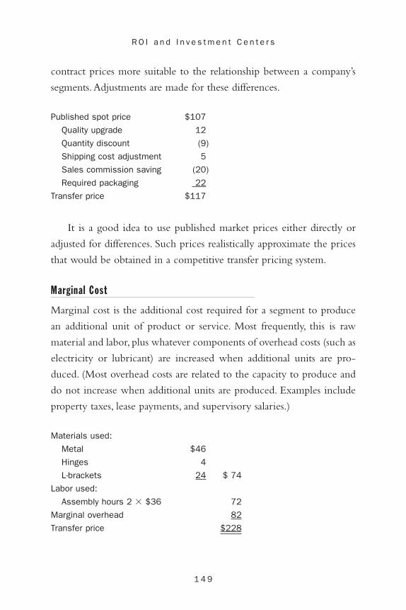
1 4 9
R O I a n d I n v e s t m e n t C e n t e r s
contract prices more suitable to the relationship between a company’s
segments.Adjustments are made for these differences.
Published spot price $107
Quality upgrade 12
Quantity discount (9)
Shipping cost adjustment 5
Sales commission saving (20)
Required packaging 22
Transfer price $117
It is a good idea to use published market prices either directly or
adjusted for differences. Such prices realistically approximate the prices
that would be obtained in a competitive transfer pricing system.
Marginal Cost
Marginal cost is the additional cost required for a segment to produce
an additional unit of product or service. Most frequently, this is raw
material and labor, plus whatever components of overhead costs (such as
electricity or lubricant) are increased when additional units are pro-
duced. (Most overhead costs are related to the capacity to produce and
do not increase when additional units are produced. Examples include
property taxes, lease payments, and supervisory salaries.)
Materials used:
Metal $46
Hinges 4
L-brackets 24 $ 74
Labor used:
Assembly hours 2 � $36 72
Marginal overhead 82
Transfer price $228

EXHIBIT 6 .6
Transfer Prices and ProfitType of Amount of Total Cost Profit (Loss) Transfer Price Transfer Price per Unit per UnitMarginal cost $228.00 $336.00 ($108.00)
Full cost $336.00 $336.00 0.00
Marginal cost plus
markup (65%) $376.20* $336.00 $40.20
Full cost plus markup
(30%) $436.80** $336.00 $100.80* $228 � 1.65 = $376.20.** $336 � 1.30 = $436.80.
1 5 0
E S S E N T I A L S o f C o r p o r a t e P e r f o r m a n c e M e a s u r e m e n t
Marginal costs are useless in calculating profit produced by the seg-
ment producing the transferred product because the total cost of pro-
duction will always include capacity costs above the marginal cost of
production (as illustrated in Exhibit 6.6 and the full-cost example that
follows). Marginal cost provides information useful for short-term oper-
ating decisions such as pricing for special orders or promotions. A spe-
cial order or promotion should not be priced below the total marginal
cost of production in all segments unless the company is willing to sus-
tain a loss.
Perhaps the biggest disadvantage of marginal cost as a transfer price
is that production inefficiencies are hidden and passed to downstream
segments.The inefficiencies of one segment are masked by the efficien-
cies of the next.
Full Costing
Full cost is the total (full) cost required for a segment to produce a prod-
uct or service, consisting of raw material, labor, and an allocated portion
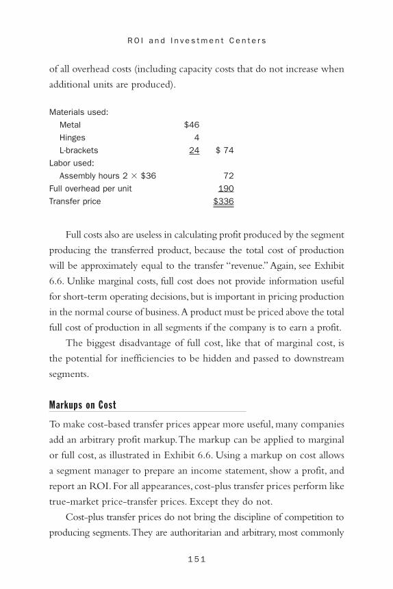
1 5 1
R O I a n d I n v e s t m e n t C e n t e r s
of all overhead costs (including capacity costs that do not increase when
additional units are produced).
Materials used:
Metal $46
Hinges 4
L-brackets 24 $ 74
Labor used:
Assembly hours 2 � $36 72
Full overhead per unit 190
Transfer price $336
Full costs also are useless in calculating profit produced by the segment
producing the transferred product, because the total cost of production
will be approximately equal to the transfer “revenue.” Again, see Exhibit
6.6. Unlike marginal costs, full cost does not provide information useful
for short-term operating decisions, but is important in pricing production
in the normal course of business.A product must be priced above the total
full cost of production in all segments if the company is to earn a profit.
The biggest disadvantage of full cost, like that of marginal cost, is
the potential for inefficiencies to be hidden and passed to downstream
segments.
Markups on Cost
To make cost-based transfer prices appear more useful, many companies
add an arbitrary profit markup.The markup can be applied to marginal
or full cost, as illustrated in Exhibit 6.6. Using a markup on cost allows
a segment manager to prepare an income statement, show a profit, and
report an ROI. For all appearances, cost-plus transfer prices perform like
true-market price-transfer prices. Except they do not.
Cost-plus transfer prices do not bring the discipline of competition to
producing segments.They are authoritarian and arbitrary, most commonly

1 5 2
E S S E N T I A L S o f C o r p o r a t e P e r f o r m a n c e M e a s u r e m e n t
Transfer Pricing
There are various cost-based or otherwise formula-driven transferprices, but scholars tend universally to recommend having market-based transfer prices or none at all. When there is no market priceto use as a guide in setting transfer prices, using cost-based, for-mula-driven transfer prices can cause managers to take dysfunc-tional actions, contrary to the company’s overall best interests.Excess costs, for example, can be passed along to other divisionswith impunity. When the markup is a percentage of cost, inefficient,inflated costs increase the transferring manager’s profits. However,in the real world, companies use cost-based, formula-driven transferprices every day, in spite of the best theory.
T I P S & TE C H N I Q U E S
set by top management using a markup return based on the company’s ulti-
mate gross profit on sales when it sells to customers outside the company,
or some measure of the company’s or the segment’s cost of capital.Another
approach to setting segment markups is to allow segment managers to earn
the profit they think would be necessary when selling to an outside cus-
tomer. Neither approach creates a competitive market price.
Summary
The use of ROI to control and evaluate performance for an investment
center can be a great idea. However, it is important to make sure that
investment centers have certain characteristics.The center should be an
independent operating center with the manager in a position to make
most of the operating decisions.
The center should be free to buy and sell wherever the manager
thinks is most efficient and effective. The center’s costs and revenues
should be separable from the rest of the company in order to determine

1 5 3
R O I a n d I n v e s t m e n t C e n t e r s
the segment’s profit. In situations where investment centers within a
company buy and sell to each other, it is necessary to set appropriate
prices for these exchanges. Such transfer prices can be determined in a
variety of ways, including use of market prices, marginal costs, full costs,
and cost plus a markup.


CHAPTER 7
1 5 5
Return on TechnologyInvestment: ROTI and ROIT
After read ing th is chapter, you wi l l be ab le to
• Understand operations technology and infrastructure tech-nology
• Use the value chain approach to analyze the impact oftechnology investments
• Evaluate the impact of technology investment on upstreamand downstream links in the value chain
• Find available vendor models to estimate the ROI of atechnology investment
• Evaluate the effect of technology on a basic business processby determining process objectives and metrics and theeffect of technology on the process
• Understand the basic components of return on infomationtechnology, or ROIT: investment, costs, and benefits
• Determine the payback or return on a technology invest-ment (ROTI)
• Calculate the dollar-impact of an improvement in produc-tivity
Determining the expected or actual ROI for technology investments is
problematic. Often the return consists of intangible benefits that may
not be readily measured or even identified as resulting directly from a

1 5 6
E S S E N T I A L S o f C o r p o r a t e P e r f o r m a n c e M e a s u r e m e n t
specific technology investment. Federal Express invested in technology that
allowed customers to use the office computer to track shipments.Although
the cost of supplying customers tracking information may be measured
directly, what change in revenue or profit can Federal Express link directly
to this investment? Often, the return associated with a technology invest-
ment consists partly or wholly of events that did not take place. For exam-
ple, the return on an investment in a firewall consists of the savings from
hacker-generated problems and losses that did not occur. How expensive
might they have been? The return on an investment in a biometric secu-
rity device must be measured as the avoided cost of intrusions.
Typically, the best evaluation metric for capital investments is a mea-
sure of discounted cash flows, net present value (NPV), or internal rate
of return (IRR). But measures of discounted cash flow fail to capture
strategic concerns and intangible, difficult-to-measure returns, such as
customer satisfaction, manufacturing flexibility, or quality enhancement.
Assume a company, for example, used NPV or IRR to select among
several computer systems available to replace an old system.Assume, also,
that one of the choices was,“Wait until next year.” Moore’s Law predicts
that computers will double in power or halve in price every year to
eighteen months. If next year’s system reflected the predicted power
increase, or price change, the choice would invariably be “Wait.” But of
course, the NPV/IRR evaluation in future years would choose “Wait”
again, and perhaps again, and again—hardly a reasonable choice.
There is no standard algorithm or template for use in calculating the
ROI for investments in information (or other) technology. Technology
investments, particularly investments in information technology (IT),
can be divided into two investment categories: operations technology
and infrastructure technology.
An investment in operations technology creates or improves a link in an
industry value chain and as such is a critical component of a company’s

1 5 7
R e t u r n o n Te c h n o l o g y I n v e s t m e n t
operation. Examples of such operations technology investments include
the Web-auction site eBay and the virtual bookstore Amazon.com.
Investments in infrastructure technology become part of a company’s infra-
structure and benefit the company by enabling another value-added
process to operate. Examples might include investments in an intranet or
a telephone system. Returns on this type of investment are difficult to
quantify.The following sections describe these two investment categories
in greater detail.
Investments in Operations Technology
Unlike investments in infrastructure, an investment in operations tech-
nology does not create its value by enabling other processes.
Operations technology enables a primary functional component in the
company’s industry value chain and generates returns directly.
Amazon.com most certainly has significant investment in an infra-
structure that supports the business processes of ordering, receiving,
inventorying, and so forth, but Amazon.com has also invested in tech-
nology that enables its primary competency: marketing books and
other items on the Internet. An operations technology enables a criti-
cal business process that could not function without the technology.
Amazon.com could perhaps perform its generic business processes
(ordering, receiving, inventorying, and so forth) without supporting
infrastructure technology, but its Internet marketing could not operate
without its operations technology.
Investments in operations technology are best viewed and evaluated
as a strategic link in the company’s value chain. The value-chain
approach to evaluating the ROI of investments in operations technol-
ogy enables a company to see the prospective investment from the holis-
tic perspective of the industry’s entire chain of activities.

1 5 8
E S S E N T I A L S o f C o r p o r a t e P e r f o r m a n c e M e a s u r e m e n t
There are two value-orientated approaches to measuring corporate
performance: value-added costs and value chain. The easiest of these to
explain is the concept of value-added and nonvalue-added costs.
Value-Added Costs
Using this approach, management attempts, first to designate all costs as
either adding value or not adding value as viewed from the perspective
of the customer. All costs in the value-added approach are related to
some specific activity. For example, the cost of fabrication is related to
fabrication activity, and the cost of inspection is related to inspection
activity. Thus, fabrication adds value as perceived by the customer
because without fabrication, there is no product to benefit the cus-
tomer. Fabrication creates value for the customer and is a value-added
activity.
Inspection, on the other hand, creates no value for the customer that
would not be created during the fabrication activity, if the activity had
been done correctly the first time.There is no value created for the cus-
tomer when a fabrication error is made.The subsequent identification
of the error by inspection does not change the value of the error, nor
does rework to restore the fabrication to specification. (Rework is
another nonvalue-added activity.)
An activity is value-added if it causes a change of state or the activ-
ity allows other activities to take place. Fabrication changes the state of
raw materials by changing it into pieces that are component-shaped and
prepared for assembly. Assembly is value-added because it changes the
components into a completed unit of product. Assembly allows the
product to be painted, and so on. Exhibit 7.1 contains a listing of
selected value-added and nonvalue-added activities.

1 5 9
R e t u r n o n Te c h n o l o g y I n v e s t m e n t
EXHIBIT 7 .1
Value-Added and Nonvalue-Added CostsExamples of Value-Added Costs
Fabricating
Assembling
Painting
Machining
Cutting
Polishing
Examples of Nonvalue-Added Costs
Inspection
Rework
Scrap
Set-ups
Billing
Paying
Collecting
Once nonvalue-added activities are identified, management tries
to reduce the amount of the nonvalue-added activity. Ultimately, the
nonvalue-added activity should be completely eliminated and its cost
driven to zero. Technology investments often offer the best route to
decreasing or eliminating a nonvalue-added activity, and, hence, the
nonvalue-added cost. Converting fabrication to a robotics operation
1 6 0
E S S E N T I A L S o f C o r p o r a t e P e r f o r m a n c e M e a s u r e m e n t
may result in products made to such uniform standards that inspection
is no longer necessary.
The value-added approach to improving profits looks only at the
company internally. As nonvalue-added costs are eliminated, by tech-
nology or otherwise, the cost of creating value is reduced and profit is
enhanced.A corollary goal is to increase the value the company adds to
the product so that the customer receives more value for the same price
(improving the company’s competitive position) or, better, at an
increased selling price. The exacting standards of robotic manufacturing
that eliminated the need for inspections may also result in an increase in
the quality (value) of the end product.
Value Chain and Operations Technology
The value-chain approach considers all activities or business processes
taking place between the creation of the raw material used in the prod-
uct, and the final consumption of the product by the customer. The
value chain of a paint manufacturer might look as shown in Exhibit 7.2.
The first link in the value chain is an oil exploration company that drills
a well in Kuwait and strikes oil, producing the raw material for the
chain.The next link is the tanker that brings the oil to the United States
so that a third link, the refinery, can process the oil into dozens of use-
ful petroleum products. Several of these components are useful directly
in paint manufacturing and others are sold by a chemical company (the
fourth link) to a company (the fifth link) that manufactures polymers
used in paint manufacture. In the sixth link in the value chain, these
polymers are used in manufacturing paint.The finished paint is sold to
a paint retailer who, in turn, sells it to a contractor who uses it to paint
a house for a homeowner, the ninth and final link.
A company might perform all the operations in its value chain, or
any combination of the links. For instance, the paint manufacturer might

1 6 1
R e t u r n o n Te c h n o l o g y I n v e s t m e n t
EXHIBIT 7 .2
The Value Chain of a Paint Manufacturer
Oil Exploration/Drilling
Tanker Transportation
Refinery Processing
Chemical Sales
Polymer Manufacturer
Paint Manufacturer
Paint Retailer
Paint Contractor
Final Customer
do nothing more than manufacture paint, or it might also have a series
of retail paint stores that sell its brand. Frequently, the same company does
the manufacture of both the paint and the polymer.Employees and man-
agers in each link in the value chain must think of ways to increase value
to the final customer. The refinery may alter its process to produce
chemicals that perform better in paint, increasing the warranty the
retailer can offer the contractor, and the contractor can offer the home-
owner. The whole value chain benefits when better value is delivered to
the final customer, regardless of whether the chain consists of one com-
pany performing nine functions, or nine companies each performing one
function.
The value-chain approach encourages managers to think outside of
the box. Investments in technology,whether IT or other technology,must
be made with an eye on the whole value chain. Often, the benefits are
not linked directly to the technology application, but may be second-,
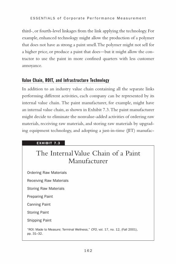
1 6 2
E S S E N T I A L S o f C o r p o r a t e P e r f o r m a n c e M e a s u r e m e n t
EXHIBIT 7 .3
The Internal Value Chain of a PaintManufacturer
Ordering Raw Materials
Receiving Raw Materials
Storing Raw Materials
Preparing Paint
Canning Paint
Storing Paint
Shipping Paint
“ROI: Made to Measure; Terminal Wellness,” CFO, vol. 17, no. 12, (Fall 2001), pp. 31–32.
third-, or fourth-level linkages from the link applying the technology. For
example, enhanced technology might allow the production of a polymer
that does not have as strong a paint smell.The polymer might not sell for
a higher price, or produce a paint that does—but it might allow the con-
tractor to use the paint in more confined quarters with less customer
annoyance.
Value Chain, ROIT, and Infrastructure Technology
In addition to an industry value chain containing all the separate links
performing different activities, each company can be represented by its
internal value chain. The paint manufacturer, for example, might have
an internal value chain, as shown in Exhibit 7.3.The paint manufacturer
might decide to eliminate the nonvalue-added activities of ordering raw
materials, receiving raw materials, and storing raw materials by upgrad-
ing equipment technology, and adopting a just-in-time (JIT) manufac-
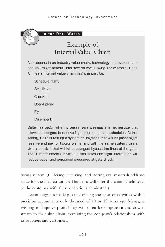
1 6 3
R e t u r n o n Te c h n o l o g y I n v e s t m e n t
Example of Internal Value Chain
As happens in an industry value chain, technology improvements inone link might benefit links several levels away. For example, DeltaAirlines’s internal value chain might in part be:
Schedule flight
Sell ticket
Check in
Board plane
Fly
Disembark
Delta has begun offering passengers wireless Internet service thatallows passengers to retrieve flight information and schedules. At thiswriting, Delta is testing a system of upgrades that will let passengersreserve and pay for tickets online, and with the same system, use avirtual check-in that will let passengers bypass the lines at the gate.The IT improvements in virtual ticket sales and flight information willreduce paper and personnel pressures at gate check-in.
I N T H E RE A L WO R L D
turing system. (Ordering, receiving, and storing raw materials adds no
value for the final customer: The paint will offer the same benefit level
to the customer with these operations eliminated.)
Technology has made possible tracing the costs of activities with a
precision accountants only dreamed of 10 or 15 years ago. Managers
wishing to improve profitability will often look upstream and down-
stream in the value chain, examining the company’s relationships with
its suppliers and customers.
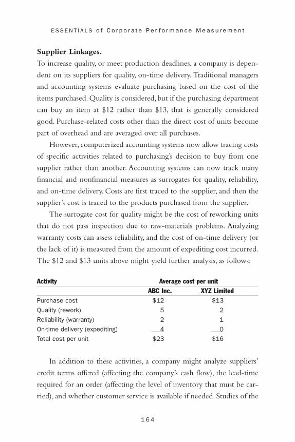
1 6 4
E S S E N T I A L S o f C o r p o r a t e P e r f o r m a n c e M e a s u r e m e n t
Supplier Linkages.
To increase quality, or meet production deadlines, a company is depen-
dent on its suppliers for quality, on-time delivery. Traditional managers
and accounting systems evaluate purchasing based on the cost of the
items purchased. Quality is considered, but if the purchasing department
can buy an item at $12 rather than $13, that is generally considered
good. Purchase-related costs other than the direct cost of units become
part of overhead and are averaged over all purchases.
However, computerized accounting systems now allow tracing costs
of specific activities related to purchasing’s decision to buy from one
supplier rather than another. Accounting systems can now track many
financial and nonfinancial measures as surrogates for quality, reliability,
and on-time delivery. Costs are first traced to the supplier, and then the
supplier’s cost is traced to the products purchased from the supplier.
The surrogate cost for quality might be the cost of reworking units
that do not pass inspection due to raw-materials problems. Analyzing
warranty costs can assess reliability, and the cost of on-time delivery (or
the lack of it) is measured from the amount of expediting cost incurred.
The $12 and $13 units above might yield further analysis, as follows:
Activity Average cost per unit ABC Inc. XYZ Limited
Purchase cost $12 $13
Quality (rework) 5 2
Reliability (warranty) 2 1
On-time delivery (expediting) 4 0
Total cost per unit $23 $16
In addition to these activities, a company might analyze suppliers’
credit terms offered (affecting the company’s cash flow), the lead-time
required for an order (affecting the level of inventory that must be car-
ried), and whether customer service is available if needed. Studies of the

1 6 5
R e t u r n o n Te c h n o l o g y I n v e s t m e n t
additional costs related to purchases might reveal that when all costs are
traced to specific suppliers, purchase cost per unit and a uniform over-
head rate is not the best method for evaluating purchasing performance
or choosing suppliers.
Customer Linkages.
Traditional function-based accounting systems assign customer costs
averaged over all customers, often as a percent of revenue. Managers
cannot use the cost system to distinguish between profitable and non-
profitable customers.
Technology has resulted in accounting systems that track customer
costs as dollars per order and analyze the value-chain link between a
company and its customers. Customer costs are a smaller percentage of
revenues for large orders, a higher percentage for small orders.Additional
considerations include terms required, lead time of orders, customer ser-
vice required, and the volatility of the customer’s demand. Managers may
also trace other costs of small-order filling, as small batch set-up, inspec-
tion, and so forth.
Companies can use the costs of different classes of customers to
focus their marketing efforts and to decide on the level of surcharges
where necessary. Banks have used this type of analysis to establish the
account privileges and charges for different types of account. Profitable
customers may be rewarded with special privileges and waived charges.
Unprofitable account classes can be structured to pay their way through
reduced privileges and account charges.
Infrastructure ROIT Model
Infrastructure refers to the basic structure of a business. ROI for any infra-
structure component, technology-based or not, is usually difficult to
quantify.What is the ROI, for instance, of the elevators and escalators?
Of the climate-control system? RSA Security notes that infrastructure
1 6 6
E S S E N T I A L S o f C o r p o r a t e P e r f o r m a n c e M e a s u r e m e n t
investments, in general, are not subject to ROI evaluation.3 For exam-
ple, a company does not base its investment in elevators and escalators
on any projected return. These infrastructure components are simply
recognized as necessary. For many companies, IT and other operations
technologies can no longer be viewed as support functions, but must be
recognized as essential business infrastructure components. Nonetheless,
many IT directors and others wanting to make IT investments find
themselves faced with the task of developing a quantifiable ROI, or,
specifically for IT investments, ROIT.
The ROI model for technology investments is still evolving.Despite
this, IT managers who request additional investment in technology are
finding they must prepare an estimated ROI as part of the process.
Often, expected ROIT is the single most important metric in the pro-
posal. Thus, IT managers are faced with an amorphous problem, with
many tangible and intangible costs and benefits that might be included
in calculating an expected ROI.
Guidelines and Estimators
Guidelines for potential customers to use in developing or estimating a
ROIT have been developed by many companies that market IT systems
or components, including IBM,Cisco Systems,Microsoft, and many oth-
ers.These guidelines are frequently available on the companies’ Web sites
and may be accompanied (or replaced) by an automated ROI estimator for
customers to use in calculating ROIT.The ROI estimator leads a poten-
tial customer through an often comprehensive series of questions that
probe the areas that might be benefited by a specific product or product
class (servers, selling, security systems, and so on).Both the guidelines and
the ROI calculators contain lists of tangible and intangible costs and
advantages specifically related to the products marketed by the company
offering the material, and might not be applicable in their entirety to
decisions involving the purchase of a different class of assets.

1 6 7
R e t u r n o n Te c h n o l o g y I n v e s t m e n t
Still, the models available from venders are useful in several ways.
Often all or part of the returns associated with a particular technology
investment may occur in another process, upstream or downstream in
the company’s value chain, or may derive from events that were avoided
and are difficult to identify. A vendor ROIT models’ value depends on
how comprehensive the set of questions is and how well these questions
cover the specific application. Regardless, guidance from venders is use-
ful in at least two areas:
1. Providing an extensive list of events that, as a result of a specific
investment, have financial impact, positive or negative
2. Suggesting default values/cost estimates for financial impacts that
are subjective and difficult to identify
Lucent Technologies’ Web site (www.lucent.com) contains Lucent’s
Telechoice ROI calculator. The calculator contains a listing of events
that affect ROI and default values calculated by Lucent, presumably
based on Lucent’s experience.There are separate macros for calculating
ROI for small business, medium business, and large business. For one
area targeted in Lucent’s marketing, managed security—small business,
Lucent’s ROI calculator offers (among other information) estimated
Service Take Rates for clients of Lucent’s customers for different ser-
vices.The ROI calculator requires input for three years. For site man-
agement, Lucent offers take-rate default values of 40 percent, 45
percent, and 50 percent for each of the three years, respectively. The
Lucent estimated default values for the percentages of customers who
will take firewall access control are 10 percent, 12 percent, and 24 per-
cent for three years. The monthly price per managed site should be
$150 (the default value). The monthly price for firewall access control
should be $50.
Potential system purchasers can accept the default values in Lucent’s
ROI calculator,or override them with their own input amounts.Once the

1 6 8
E S S E N T I A L S o f C o r p o r a t e P e r f o r m a n c e M e a s u r e m e n t
Value ChainCheck carefully to see what time period is used when returns arecalculated on technology investments. Calculations of ROIT are fre-quently made for a period spanning several years because IT invest-ments typically offer poor or negative returns in the first year. Ratherthan describing an investment as returning a negative return the firstyear, and a positive return thereafter, the investment is described ascreating a cumulative positive return in three years.
For example, the default values for a small business in the LucentTechnologies Telechoice ROI calculator yield a negative cash flow of$3,005,675 in year one, then positive cash flows of $10,187,261and $48,243,529 the second and third years, respectively, yieldinga cumulative 504 percent IRR over three years.
T I P S & TE C H N I Q U E S
input of likelihoods, events, costs, and prices is complete, the ROI calcu-
lator prepares pro forma income statements for three years, with an inter-
nal rate of return for the three years and a three-year net present value.
The Value of Performing a ROIT Analysis
Investment in IT is more frequently tactical than strategic. For example,
when accounting spreadsheets first became available, companies that
used the software received a definite advantage. The advantage was par-
ticularly evident in budgeting and planning. Companies using spread-
sheet software could prepare multiple iterations of a budget at different
activity levels—sales at $1 million, sales at $1.2 million—to see the effect
on profits and costs. Sensitivity analyses that were difficult or impracti-
cal manually were simple to calculate using spreadsheet software. But, as
time passed, spreadsheet software became less expensive and more com-
mon.Ultimately, automated spreadsheets were the standard, and companies
that used the software no longer had an advantage. Instead, companies that

1 6 9
R e t u r n o n Te c h n o l o g y I n v e s t m e n t
Use of an ROI Calculator
Before deciding to use a particular vendor’s proprietary ROI calcu-lator to estimate the potential value of an IT investment, considerthe vendor’s history with the application under consideration. Studythe ROI calculator model to see if it captures the types of benefits,savings, and costs relevant to your own company and its operations.Is the model as sophisticated as needed? Who created it? The ven-dor? A consulting firm? Do you need to add effects not consideredin the model? Does the time horizon of the model match the patternof your intended use? Calculating a five-year ROI might not be ade-quate for an application expected to be obsolete in three years.Finally, if two or more vendors offer ROI calculators, evaluate yourapplication using each model.
I N T H E RE A L WO R L D
did not adopt automated spreadsheets were at a definite disadvantage. As
technology increases, failure to “get aboard” when a new development
becomes available may result not only in the loss of a tactical advantage,
but a failure to remain competitive.
Thus, it is important that the costs of making a new or improved IT
investment be compared with the cost of not making the investment, in
terms of lost tactical advantage and ultimately, competitive advantage.
There is frequently the argument that it is better to wait on the next
generation of whatever technology is considered and the feeling that
when the next generation arrives, perhaps the company should not be
happy with “old” technology. Nonetheless, however advanced the new
generations become, it makes no difference if the company’s old IT sys-
tem still satisfies its needs.
Cisco Systems maintains that the evaluation process itself has bene-
fits that make the exercise worth the effort, even if no new technology

1 7 0
E S S E N T I A L S o f C o r p o r a t e P e r f o r m a n c e M e a s u r e m e n t
is added.4 Cisco is addressing an evaluation by a company considering
the purchase of high-availability networking, but the benefits are suffi-
ciently generic to apply to other in-depth system evaluations:
• A better understanding of the IT within company’s businessmodel and the costs and revenues affected by the level of ITperformance
• Quantifiable data and metrics that managers can use indecision making and planning
• The ability to perform what-if analysis of the consequences ofdifferent scenario relating to the IT area evaluated
• A better buy-in to the mission and operation of the ITfunction by non-IT managers who must participate in anevaluation
• The ability to compare future performance to expectations,whether the investment is made or not
• An improved ability to react to unanticipated events thatrequires the use or involvement of IT
Measuring the Impact of Technology Investment
Measuring the impact of IT investment is difficult because so much of the
effect of an infrastructure component is tied inseparably to the business
operation or process enabled by the infrastructure. A business process is
defined loosely as a group of activities addressing the same objective.
Before accepting a list of events as measuring the impact of technology
investment, managers should insist that the metrics follow directly from
the activities in the business process and address one or more of the objec-
tives of the process.Thus, metrics used to evaluate ROIT should be based
on both the basic business process affected, and the related business objec-
tive(s).5
An example of a basic business process is sales to customers. A list of
related business objectives would include maximizing online sales to exist-

1 7 1
R e t u r n o n Te c h n o l o g y I n v e s t m e n t
ing customers. Potential metrics used to measure progress toward this
objective include the following:
• Proportion of sales generated online
• Proportion of existing customers purchasing online
• Sales drop-off rate
• Repeat business rate
• Percent change in the size of the average online sale
This metric and others are described in Exhibit 7.4.
Once an IT manager has considered the basic process of making sales
to customer, and has developed metrics to address the objective maximiz-
ing online sales to existing customers, an IT manager can ask such impact
questions as,“What if we use encryption to secure communication with
customers and accept orders with digital signatures rather than requiring
them to print, process and mail an order form?”“What if we establish a
24/7 hotline to answer customer’s questions?” “What if we establish a
tracking system that will allow customers to track their orders online?”
Examining the expected impact of these questions on the metrics
developed should assist managers in recognizing and quantifying the
returns on the required investment. If, for example, establishing an
online order-tracking system would require an additional $40,000 server
but could be expected to double the proportion of sales generated
online and increase by 50 percent the proportion of existing customers
purchasing online, the IT manager is prepared to develop a range of
expected returns and the metrics by which the returns can be measured.
The Components of ROIT: Investment, Costs, and Benefits
Three components are necessary to measure return on technology
investment: investment, costs, and benefits.

1 7 2
E S S E N T I A L S o f C o r p o r a t e P e r f o r m a n c e M e a s u r e m e n t
EXHIBIT 7 .4
Processes, Objectives, and Metrics
BUSINESS PROCESS
sales to customers
BUSINESS OBJECTIVES
maximizing online sales to existing customers
POTENTIAL METRICS
proportion of sales generated online
proportion of existing customers purchasing online
sales drop-off rate
repeat business rate
percent change in the size of the average online sale
BUSINESS PROCESS
sales to customers
BUSINESS OBJECTIVES
minimizing cost of acquiring new customers
POTENTIAL METRICS
percent of new customers online
cost of each new customer
BUSINESS PROCESS
sales to customers
BUSINESS OBJECTIVES
maximizing customer satisfaction

1 7 3
R e t u r n o n Te c h n o l o g y I n v e s t m e n t
EXHIBIT 7 .4
PR O C E S S E S , OB J E C T I V E S , A N D ME T R I C S C O N T I N U E D
POTENTIAL METRICS
number of incorrect orders shipped
number of help line calls
number of exchanges
BUSINESS PROCESS
sales to customers
BUSINESS OBJECTIVES
maximizing customer satisfaction
POTENTIAL METRICS
number of incorrect orders shipped
proportion of incorrect orders shipped
number of help line calls per sales dollar
number of exchanges per sales dollar
BUSINESS PROCESS
product development
BUSINESS OBJECTIVES
improve response to changing market conditions
POTENTIAL METRICS
order cycle time
order delivery time
product time to market
time to change product
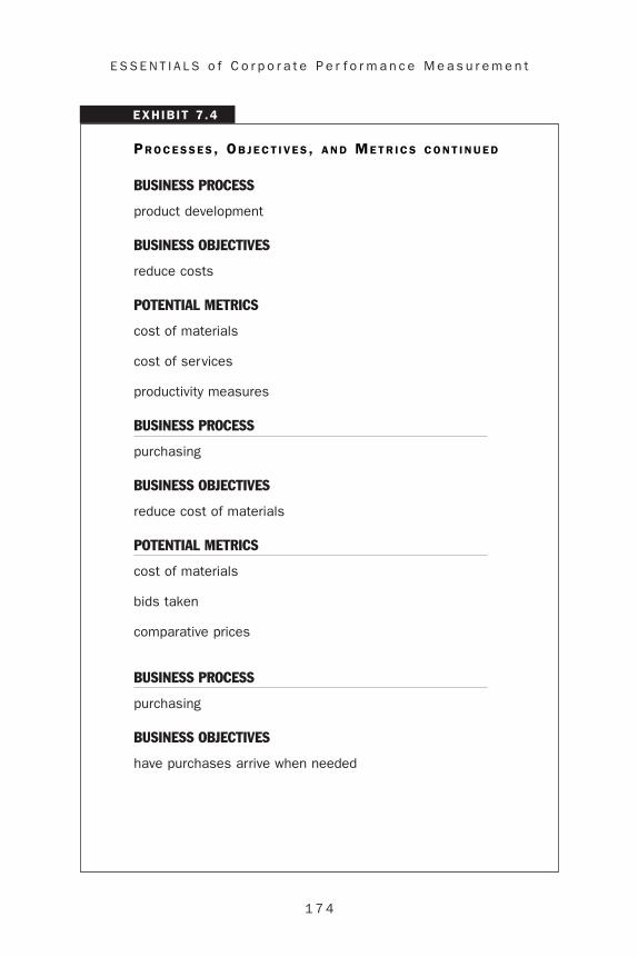
1 7 4
E S S E N T I A L S o f C o r p o r a t e P e r f o r m a n c e M e a s u r e m e n t
EXHIBIT 7 .4
PR O C E S S E S , OB J E C T I V E S , A N D ME T R I C S C O N T I N U E D
BUSINESS PROCESS
product development
BUSINESS OBJECTIVES
reduce costs
POTENTIAL METRICS
cost of materials
cost of services
productivity measures
BUSINESS PROCESS
purchasing
BUSINESS OBJECTIVES
reduce cost of materials
POTENTIAL METRICS
cost of materials
bids taken
comparative prices
BUSINESS PROCESS
purchasing
BUSINESS OBJECTIVES
have purchases arrive when needed

1 7 5
R e t u r n o n Te c h n o l o g y I n v e s t m e n t
EXHIBIT 7 .4
PR O C E S S E S , OB J E C T I V E S , A N D ME T R I C S C O N T I N U E D
POTENTIAL METRICS
shortage caused downtime
lead-time allowed
average inventory levels
inventory level at each orderpoint
This exhibit is based on RSA Security, PKI and Return on Investment, 2001,available at www.RSASecurity.com, pp. 1–3.
Investment
The required capital investment is perhaps the easiest component to
measure accurately. The investment costs typically include one or more
of the following costs:
• Hardware
• Software
• Facility modifications
• Training for employees
• Consultant’s fees
• Recruiting cost of new employees
In a study of retail e-commerce, IBM classified the investment initia-
tives of online ventures as focused either short-term or long-term. Sixty-
three percent of the companies studied had a primary short-term
investment focus. These companies focused on immediate results and
rarely made investments larger than projected cash inflows. The remain-
ing companies had a primarily long-term orientation and focused on
becoming profitable in one or two years, following initial short-term

1 7 6
E S S E N T I A L S o f C o r p o r a t e P e r f o r m a n c e M e a s u r e m e n t
losses. Companies focusing on long-term profitability invested signifi-
cantly larger amounts than companies with a short-term focus and
received significantly higher returns. IBM felt retailers that stressed imme-
diate returns damaged their business by focusing on short-term ROI.6
Benefits
IT investment typically addresses the improvement of a basic business
process by accomplishing one or more of the objectives related to that
process. The benefits may be measured by the metrics shown in Exhibit
7.4.The benefits of new IT investment might thus be tangible or intan-
gible and may result in increased revenues, reduced costs, and/or losses
avoided.
In discussing hardware for high-availability networking, Cisco
Systems advises companies to include the risk of not upgrading hard-
ware and, because of that decision, losing business from network out-
ages. High-availability refers to five nines availability—systems that are
available 99.999 (or greater) percent of the time.A company that is four
nines or three nines is not competitive.
Costs
Like benefits, costs can be tangible or intangible, and can relate to suc-
cess or lack of success in accomplishing operating or strategic objectives.
Intangible costs are much more difficult to quantify than are intangible
benefits. Lost revenue from a system outage that impacts sales, such as an
Internet merchant losing sales, may be objectively estimated, but the
cost of frustrated customers is difficult to quantify. The direct cost of
replacing an incorrect shipment may be in the accounting records, but
the cost of damage to the company’s reputation is unknown. IT-related
costs might include any of the following:

1 7 7
R e t u r n o n Te c h n o l o g y I n v e s t m e n t
• Direct operating expenditures (as salaries or energy costs)
• Indirect losses (as lost revenue or changes in stock prices ordebt rating)
• Direct losses (as lawsuits resulting from failure to perform)
• Lost or forfeited revenue (as from customer turnover)
When the costs of quality are measured for a total quality manage-
ment report, experts believe that the true cost of a product’s external
failure is 4 to 10 times as great as the product’s measurable external fail-
ure costs. A failure cost of $1,000,000 in the accounting records for
replacing defective units shipped may actually cost the company
$4,000,000 to $10,000,000 in total losses. Although the order of mag-
nitude has not been studied, the same phenomenon is no doubt present
in e-business failures.
Payback
Payback is a frequently cited metric used in making investments in IT.
Payback is a simple concept:A system that costs $100,000 and generates
$20,000 per year in profit or savings will pay for itself in five years.
payback period = investment/average annual profit or saving
Payback is not a preferred method for making capital investment
decisions. Payback ignores the total benefits of an investment—will the
$20,000 annual return continue past five years? An investment that will
return $20,000 per year for 5 years has the same payback as an invest-
ment that returns $20,000 annually for 50 years. Likewise, payback
ignores the time value of money. An investment that returns $20,000
each of five years has the same payback as an investment that returns
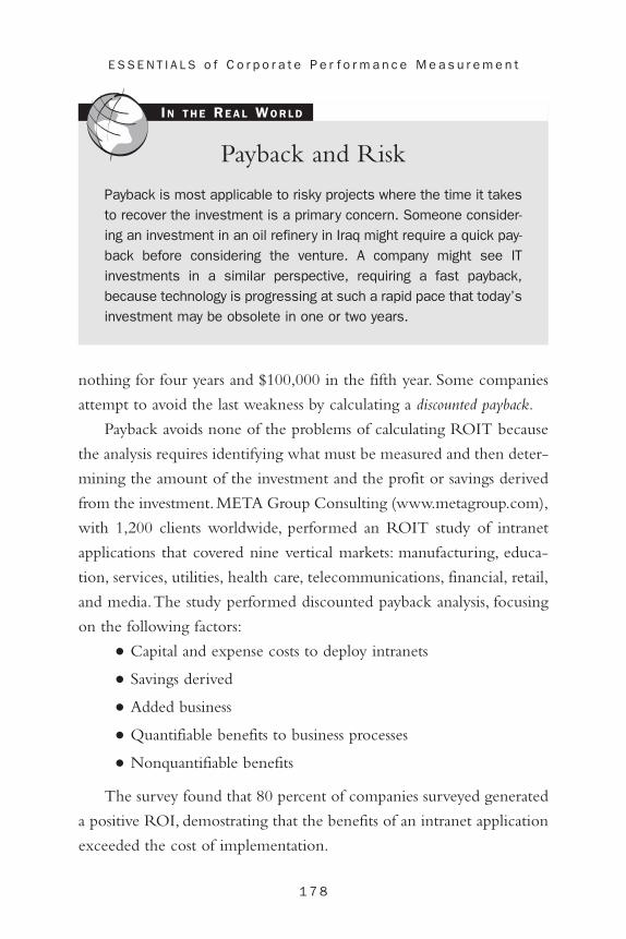
1 7 8
E S S E N T I A L S o f C o r p o r a t e P e r f o r m a n c e M e a s u r e m e n t
Payback and Risk
Payback is most applicable to risky projects where the time it takesto recover the investment is a primary concern. Someone consider-ing an investment in an oil refinery in Iraq might require a quick pay-back before considering the venture. A company might see ITinvestments in a similar perspective, requiring a fast payback,because technology is progressing at such a rapid pace that today’sinvestment may be obsolete in one or two years.
I N T H E RE A L WO R L D
nothing for four years and $100,000 in the fifth year. Some companies
attempt to avoid the last weakness by calculating a discounted payback.
Payback avoids none of the problems of calculating ROIT because
the analysis requires identifying what must be measured and then deter-
mining the amount of the investment and the profit or savings derived
from the investment. META Group Consulting (www.metagroup.com),
with 1,200 clients worldwide, performed an ROIT study of intranet
applications that covered nine vertical markets: manufacturing, educa-
tion, services, utilities, health care, telecommunications, financial, retail,
and media.The study performed discounted payback analysis, focusing
on the following factors:
• Capital and expense costs to deploy intranets
• Savings derived
• Added business
• Quantifiable benefits to business processes
• Nonquantifiable benefits
The survey found that 80 percent of companies surveyed generated
a positive ROI, demostrating that the benefits of an intranet application
exceeded the cost of implementation.

1 7 9
R e t u r n o n Te c h n o l o g y I n v e s t m e n t
Changes in Productivity
Improvements in productivity are an often cited metric for evaluating
returns on technology investment. Determining dollar amounts result-
ing from a change in productivity is not straightforward, however.
Productivity is measured as output per unit of input.
productivity rate = output/input
If a company, in fiscal year 1, generates $10,000,000 in online sales
with hardware lease costs of $550,000, productivity of the hardware is
measured as follows:
If in fiscal year 2 the company generated $12,000,000 in sales with
additional IT hardware lease cost of $50,000 ($600,000 total), is there an
improvement in productivity?
Yes, productivity increased from 18.18 to 20.0. But by what dollar
amount? To determine a dollar amount, we must restate the productiv-
ity equation so that we solve for inputs rather than the rate.
Now we can compare the inputs that would be required in fiscal
year 2 if we had performed at the productivity rate of fiscal year 1.
inputs � output>productivity rate
1Productivity rate 2 1 inputs 2 � output
productivity rate � output>input
productivity rate 12 2 � 20.0
productivity rate 12 2 � $12,000,000>$600,000
productivity rate 11 2 � 18.18
productivity rate 11 2 � $10,000,000>$550,000
productivity rate � online sales>hardware costs

1 8 0
E S S E N T I A L S o f C o r p o r a t e P e r f o r m a n c e M e a s u r e m e n t
Because productivity increased in fiscal year 2, an output of
$12,000,000 was produced with only $600,000 rather than the
$660,066 that would have been required at the fiscal year 1 productiv-
ity rate.The increase in productivity produced savings of $60,066 at an
additional cost of $50,000.The $50,000 produced an ROIT of 20.132
percent.
Theoretical input required in fiscal year 2 $660,066
Actual input required (600,000)
Savings (reduction in input) $ 60,066
New investment (50,000)
Savings from productivity increase $ 10,066
ROIT = Savings/new investment = $10,066/$50,000 = 20.132%
Summary
Measuring the return on technology investments is not a straightforward
procedure. Returns are often intangibles that are difficult to measure
objectively, or may occur in parts of the value chain different from the
link where the investment is made. Still, returns on technology invest-
ments must be quantified before many companies will allow technology
investment.The value chain affords a viable approach to examining the
companywide and even industrywide returns to be generated on invest-
ments on technology. For infrastructure ROIT, it is useful to develop
objectives and metrics directly from the basic business processes. Once
the objectives and metrics are developed, impact statements can be ana-
lyzed and investment-generated returns estimated.
inputs required � $660,066
inputs required � $12,000,000>18.18
inputs required � output 12 2>productivity rate 11 2

1 8 1
R e t u r n o n Te c h n o l o g y I n v e s t m e n t
Payback is a statistic useful in evaluating technology because it is a
measure of exposure to risk in an environment where rapid change is
expected. Increases in productivity are a frequently cited metric used to
evaluate the success of technology investments. This chapter explains
the algorithms for both measures.

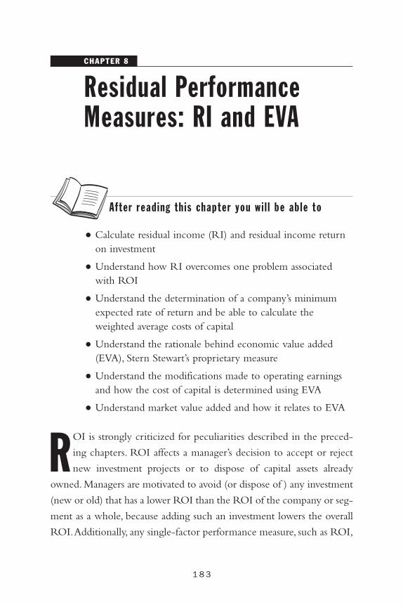
After read ing th is chapter you wi l l be ab le to
• Calculate residual income (RI) and residual income returnon investment
• Understand how RI overcomes one problem associatedwith ROI
• Understand the determination of a company’s minimumexpected rate of return and be able to calculate theweighted average costs of capital
• Understand the rationale behind economic value added(EVA), Stern Stewart’s proprietary measure
• Understand the modifications made to operating earningsand how the cost of capital is determined using EVA
• Understand market value added and how it relates to EVA
ROI is strongly criticized for peculiarities described in the preced-
ing chapters. ROI affects a manager’s decision to accept or reject
new investment projects or to dispose of capital assets already
owned. Managers are motivated to avoid (or dispose of ) any investment
(new or old) that has a lower ROI than the ROI of the company or seg-
ment as a whole, because adding such an investment lowers the overall
ROI.Additionally, any single-factor performance measure, such as ROI,
CHAPTER 8
1 8 3
Residual PerformanceMeasures: RI and EVA

1 8 4
E S S E N T I A L S o f C o r p o r a t e P e r f o r m a n c e M e a s u r e m e n t
can produce dysfunctional behavior when a manager attempts to max-
imize the single-factor measure. For example, maintenance or other
necessary expenditures may be delayed to increase a period’s ROI at the
expense of the company’s overall health and the ROI next period.
There are two residual profitability measures structured to avoid the
deficiencies of ROI and other single-factor measures. Residual income
(RI) is a simple measure of the returns that an entity generates above a
minimum required rate of return, often the company’s cost of capital.
Economic value added (EVA) is a much more elaborate measure of a com-
pany’s ability to increase the wealth of its owners. EVA is a proprietary
measure copyrighted by Stern Stewart and has recently received a great
deal of attention.
Residual Income
Residual income is thought to avoid the incongruent goals of managers
who seek to avoid projects that have a lower ROI than the company or
segment ROI. Segment managers are often charged for capital commit-
ted to their segments. If managers are not charged for capital, there is, at
least, a minimum or hurdle rate that investments are expected to exceed.
This rate is frequently the weighted average cost of capital. RI looks at
the profit contributed by an investment above its cost of capital or min-
imum rate of return.
RI is the income earned in excess of a minimum rate of return. If
the manager of a company or segment that creates a ROI of 25 percent
evaluates a new investment that returns only 20 percent, the manager
may refuse the project to avoid decreasing the overall ROI. However, if
an investment is evaluated using RI and a 15 percent minimum rate of
return, the manager will realize that adopting the project increases total
earnings. Here, the $6,250 increase in RI justifies the reduction in ROI.

1 8 5
R e s i d u a l P e r f o r m a n c e M e a s u r e s
Before New New With New Project Project Project
Investment $500,000 $125,000 $625,000
Profit 125,000 25,000 150,000
Cost of capital @15% 75,000 18,750 93,750
Residual income (above cost of capital) $ 50,000 $ 6,250 $ 56,250
ROI 25% 20% 24%
One problem with using RI for performance measurement is that
it is difficult to make comparisons among segments of different sizes.
Large segments should generate larger amounts of RI than small seg-
ments. In these cases, using a budgeted or target RI for each segment
compensates for size differences—but in those cases, a budgeted ROI
that recognized the value of the 20 percent project accomplished the
same thing.
RI avoids none of the problems of ROI discussed in the earlier
chapters except the tendency to avoid an otherwise desirable investment
because it decreases a manager’s ROI.The problems defining profit and
investment are still present.
Determining a Minimum Rate of Return
The minimum rate of return acceptable for a proposed investment is
the rate of return a company would forgo by investing in project A
rather than in alternative project B, assuming the projects are of com-
parable risk. This rate should equal or exceed the company’s cost of
capital. A company’s cost of capital is the weighted average cost of all the
company’s debt and equity financing. It is the weighted average rate
that results from obtaining funds at various costs from stockholders and
creditors.The cost of debt is simply the effective interest rate of each
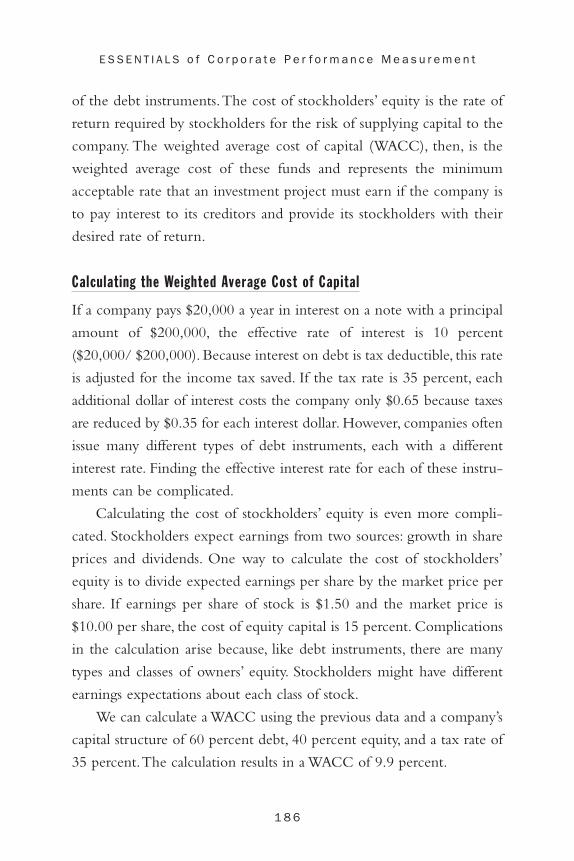
1 8 6
E S S E N T I A L S o f C o r p o r a t e P e r f o r m a n c e M e a s u r e m e n t
of the debt instruments.The cost of stockholders’ equity is the rate of
return required by stockholders for the risk of supplying capital to the
company. The weighted average cost of capital (WACC), then, is the
weighted average cost of these funds and represents the minimum
acceptable rate that an investment project must earn if the company is
to pay interest to its creditors and provide its stockholders with their
desired rate of return.
Calculating the Weighted Average Cost of Capital
If a company pays $20,000 a year in interest on a note with a principal
amount of $200,000, the effective rate of interest is 10 percent
($20,000/ $200,000). Because interest on debt is tax deductible, this rate
is adjusted for the income tax saved. If the tax rate is 35 percent, each
additional dollar of interest costs the company only $0.65 because taxes
are reduced by $0.35 for each interest dollar. However, companies often
issue many different types of debt instruments, each with a different
interest rate. Finding the effective interest rate for each of these instru-
ments can be complicated.
Calculating the cost of stockholders’ equity is even more compli-
cated. Stockholders expect earnings from two sources: growth in share
prices and dividends. One way to calculate the cost of stockholders’
equity is to divide expected earnings per share by the market price per
share. If earnings per share of stock is $1.50 and the market price is
$10.00 per share, the cost of equity capital is 15 percent. Complications
in the calculation arise because, like debt instruments, there are many
types and classes of owners’ equity. Stockholders might have different
earnings expectations about each class of stock.
We can calculate a WACC using the previous data and a company’s
capital structure of 60 percent debt, 40 percent equity, and a tax rate of
35 percent.The calculation results in a WACC of 9.9 percent.
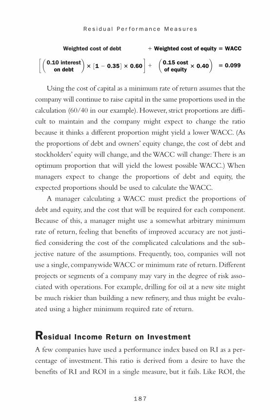
1 8 7
R e s i d u a l P e r f o r m a n c e M e a s u r e s
Using the cost of capital as a minimum rate of return assumes that the
company will continue to raise capital in the same proportions used in the
calculation (60/40 in our example). However, strict proportions are diffi-
cult to maintain and the company might expect to change the ratio
because it thinks a different proportion might yield a lower WACC. (As
the proportions of debt and owners’ equity change, the cost of debt and
stockholders’ equity will change, and the WACC will change:There is an
optimum proportion that will yield the lowest possible WACC.) When
managers expect to change the proportions of debt and equity, the
expected proportions should be used to calculate the WACC.
A manager calculating a WACC must predict the proportions of
debt and equity, and the cost that will be required for each component.
Because of this, a manager might use a somewhat arbitrary minimum
rate of return, feeling that benefits of improved accuracy are not justi-
fied considering the cost of the complicated calculations and the sub-
jective nature of the assumptions. Frequently, too, companies will not
use a single, companywide WACC or minimum rate of return. Different
projects or segments of a company may vary in the degree of risk asso-
ciated with operations. For example, drilling for oil at a new site might
be much riskier than building a new refinery, and thus might be evalu-
ated using a higher minimum required rate of return.
Residual Income Return on Investment
A few companies have used a performance index based on RI as a per-
centage of investment. This ratio is derived from a desire to have the
benefits of RI and ROI in a single measure, but it fails. Like ROI, the
Weighted cost of debt
c a0.10 intereston debt
b � 31 � 0.35 4 � 0.60 d�
�
Weighted cost of equity
a0.15 costof equity
� 0.40b� WACC
� 0.099

1 8 8
E S S E N T I A L S o f C o r p o r a t e P e r f o r m a n c e M e a s u r e m e n t
hybrid measure appears to normalize unlikes and have intuitive mean-
ing, but in truth the relationship is artificial and, because of this, gives
rise only to contrived interpretations.
For the illustration used earlier, the ratio (which has no particular
name) is as follows.
What does this mean? Only that residual income with the project
is 9.0 percent of the investment base, down from 10.0 percent
($50,000/$500,000) without the project. Any additional interpretation
is meaningless.
Economic Value Added (EVA)
Shareholders rely on information produced by accountants and on cri-
teria such as earnings per share and reported net income. But it is the
premise of the EVA calculation that both earnings per share and net
income are distorted by accounting procedures and do not give a clear
picture of a company’s performance.Accounting measures, it is alleged,
are intended to calculate earnings that are much too conservative.The
resulting reported profits are intended to tell creditors the amount of
earnings under the most pessimistic of interpretations. These earnings
amounts are structured to inform creditors how well protected they are
if the company becomes unable to pay its debts.Accounting procedures
are not designed to create financial statements that provide investors an
impartial assessment of how well the company performed.
Calculating EVA
The simple definition of EVA is economic profit.7 Proponents of EVA
maintain that stockholders are not informed by accounting measures of
residual incomeinvestment
�$56,250$625,000
� 9.0%

1 8 9
R e s i d u a l P e r f o r m a n c e M e a s u r e s
Real Use of EVA
Since the EVA concept was first introduced, more than 300 compa-nies have used it, including Coca-Cola, Quaker Oats, BoiseCascade, Briggs and Stratton, Lafarge, Siemans, Tate and Lyle,Telstra, Monsanto, JCPenney, and the U.S. Postal Service.
This information is taken from Joel M. Stern and John Shiely, The EVA Challenge,(New York: John Wiley & Sons, 2001), p. 16.
I N T H E RE A L WO R L D
profit. Instead, stockholders need to know how successful the company
is at creating new wealth. Equity is defined as property rights. There are
two types of property rights, the equity of creditors (liabilities) and the
equity of owners (stockholders’ equity). EVA is said to measure in real
terms the increase in wealth, defined as total equities—including both
creditors’ equity and stockholders’ equity. EVA is the statistic that stock-
holders need.When bonus plans use EVA rather than earnings per share
or ROI to measure the performance of managers, managers pursue
activities congruent with the interests of stockholders. Change in EVA
is the force that causes change in the market price of a company’s stock.
The equation for calculating EVA is as follows.
NOPAT is net operating profit after taxes. If a company’s NOPAT is
$3,000 and its total debt and owners’ equity are $10,000 with a 10 per-
cent cost of capital, EVA is calculated as:
EVA � $2,000
EVA � $3,000 � $1,000
EVA � $3,000 � 3$10,000 � .10 4
EVA � NOPAT � 1the cost of capital 2 � 1total debt and owners’ equity 2

1 9 0
E S S E N T I A L S o f C o r p o r a t e P e r f o r m a n c e M e a s u r e m e n t
If a company earns only enough to cover its cost of capital, it has
earned no profit. This is why the cost of capital is often a company’s
minimum desired rate of return:Anything less creates a loss.
The “net” NOPAT refers to the adjustments to operating profit after
tax that must be made to arrive at NOPAT.NOPAT might well have been
named OPATA—operating profit after taxes and adjustment. Proponents
of EVA have found 120 separate distortions of profit created by account-
ing procedures. A correction is required for each distortion present in a
company’s income calculation to arrive at NOPAT, although most com-
panies have only a few.The accounting treatment of the following items
are felt to be the most egregious distortions of reported profits and its sur-
rogate measures, such as earnings per share and the price/earnings ratio:
• Research and development. Accounting procedures require thatinvestments in research and development be expensed eachyear, as though the expenditure would provide no benefit infuture years.The simple definition of an asset is a cost that willbenefit the future, an expense being a cost that carries nofuture benefit. EVA proponents argue that expensing researchand development both understates a company’s assets andoverstates expenses, driving profits down.
• Advertising and selling. Accounting procedures likewise requirethat advertising and other selling/marketing costs be expensedwhen incurred. EVA proponents make the same argument thatexpensing these costs understates a company’s assets, overstatesexpenses, and drives profits down.
• Employee training. These costs are also expensed, failing torecognize that the future is benefited by training employees.Asa result, assets are overstated and profit is understated.
• Historical cost. Historical cost causes a different problem.Assetsare shown in the balance sheet at their original purchase cost,or at market price, whichever is lower.With even mildinflation, this causes assets to be understated. If a company

1 9 1
R e s i d u a l P e r f o r m a n c e M e a s u r e s
EXHIBIT 8 .1
Straight-Line and AcceleratedDepreciation Expense
Straight-Line Sum-of-the-Years’-DigitsDepreciation Depreciation Difference
Year (1) (2) (2) � (1)1 $2,500 $4,000 $1,500
2 2,500 3,000 500
3 2,500 2,000 (500)
4 2,500 1,000 (1,500)
Total $10,000 $10,000 -0-
purchased land on Main Street for $100,000 in 1912, and it isnow worth $10 million, it is shown on the balance sheet at$100,000.
• Deferred taxes. Accounting procedures often include as expensesamounts of deferred taxes not yet paid by a company.Althoughthese taxes might be liabilities of the company, they are notexpenses. Deducting deferred, unpaid taxes depresses profit and owners’ equity.
• Reserves. Accountants create many reserves or allowances, suchas the allowance for warranty obligations coming due in thefuture, or for bad debts not yet identified. Often these reservesare too large and unnecessarily obscure profits. SEC ChairmanArthur Levitt, Jr.8 has referred to such reserves as cookie-jarreserves. Proponents of EVA believe that warranty costs arebetter measured when a company waits until the cost is paidbefore recognizing the associated expense.
• Alternative accounting methods. Companies can frequently chooseamong alternative accounting methods, some of which affecttaxable income. Exhibit 8.1 shows the difference between

1 9 2
E S S E N T I A L S o f C o r p o r a t e P e r f o r m a n c e M e a s u r e m e n t
straight-line and accelerated sum-of-the-years’-digits (SYD)depreciation for a $10,000 machine with a four-year life andno salvage value. SYD depreciation yields higher depreciationexpense and lower net income than straight-line in the firsttwo years of the machine’s life, but the situation is exactlyreversed in the last two years. Over the machine’s four-yearlife, both methods result in the same total depreciationexpense and earnings.
Regardless of the depreciation method used for financial reporting,
a company is free, for tax reporting purposes, to use the depreciation
method that results in the lowest tax liability—so the choice of depre-
ciation method for earnings does not result in different cash flows, only
in different reported earnings. Other procedural choices require a com-
pany to use the same method for both financial reporting and taxes.The
choice of inventory methods is an example of alternative methods that
must be the same for financial reporting as for taxes. When the same
method must be used for both taxes and financial reporting, the choice
affects cash flows as well as reported profits.
Managed Earnings
Reported profits are also distorted by managers who attempt to “man-
age” earnings rather than operations.9 Managers are motivated to
increase profits, and the increase must be an acceptable size.The increase
must be at least as large as stockmarket analysts have predicted. Missing
analysts’ predictions by as little as a penny can cause the company’s stock
price to tumble.
Managers can manage profits in many ways. Managers can increase
reported profits by changing the timing of revenue and expense recog-
nition. For example, a retailer might offer liberal credit terms to entice
customers to buy who would customarily wait until next year.A com-
pany that advertises “No payment or interest until June” might motivate
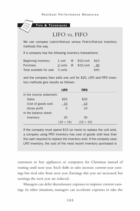
1 9 3
R e s i d u a l P e r f o r m a n c e M e a s u r e s
LIFO vs. FIFOWe can compare Last-in-first-out versus First-in-first-out inventorymethods this way.
If a company has the following inventory transactions:
Beginning inventory 1 unit @ $10/unit $10
Purchase 2 units @ $15/unit 30
Total available for sale 3 units $40
and the company then sells one unit for $20, LIFO and FIFO inven-tory methods give results as follows:
LIFO FIFOIn the income statement:
Sales $20 $20
Cost of goods sold 15 10
Gross profit 5 10
In the balance sheet:
Inventory 25 30
(10 + 15) (15 + 15)
If the company must spend $15 (or more) to replace the unit sold,a company using FIFO inventory has cost of goods sold less thanthe cash required to replace the inventory sold. If the company usesLIFO inventory, the cost of the most recent inventory purchased is
T I P S & TE C H N I Q U E S
customers to buy appliances or computers for Christmas instead of
waiting until next year. Such shifts in sales increase current-year earn-
ings but steal sales from next year. Earnings this year are increased, but
earnings the next year are reduced.
Managers can defer discretionary expenses to improve current earn-
ings. In other situations, managers can accelerate expenses to take the

1 9 4
E S S E N T I A L S o f C o r p o r a t e P e r f o r m a n c e M e a s u r e m e n t
“hit” in a current year of expected low earnings and improve prospects
for next year.Travel, maintenance or advertising expenditures might be
delayed from December, year one, to January, year two, to reduce year
one expenses. In early fall, managers might be able to set the date for
repainting the equipment and factory buildings, or for the annual sales
meeting. Delaying these expenses will improve current earnings; accel-
erating them will improve next year. Changing the timing of revenues
and expenses produces an increase in current reported earnings that
cannot be sustained in future periods.
Questionable Practices
Some efforts to manage earnings go beyond simply timing changes.
Managers might increase sales through loose credit standards that also
increase bad debts, or might bias expenses that must be based on esti-
mates, such as obsolete inventories or warranty costs to delay recogni-
tion of the full amount of these expenses. Actions such as these are
ethically questionable and result (if successful) in earnings increases in
one year at the expense of another, as the costs must eventually be writ-
ten off. Profits created by such questionable practices cannot be sus-
tained and do not provide an accompanying increased inflow of cash or
other assets.A study, years ago, by the National Accounting Association
found that straight-line depreciation is the most appropriate method for
most manufacturers.
Exhibit 8.1 shows the difference between straight-line and the
accelerated SYD depreciation for a $10,000 machine with a four-year
life.
Market Value Added
Market value added (MVA) is defined as the “difference between the mar-
ket value of a company and the sums invested in it over the years.”10 If
the market price of a company’s stock is based on expectations about

1 9 5
R e s i d u a l P e r f o r m a n c e M e a s u r e s
LIFO Reserve in the Financial Statements
Some accounting distortions can be removed if a financial state-ment user knows how. A LIFO reserve is calculated by accountantsand given in the Notes to the financial statements. The LIFO reserveis the difference between LIFO cost and the replacement cost of theinventory (usually assumed to be FIFO cost). Analysts can use theLIFO reserve to determine the effect of the LIFO/FIFO choice on thequality of earnings. For example, if ACME Company had cost ofgoods sold of $1,000,000 using LIFO and the inventory note to thefinancial statements shows a LIFO reserve of $150,000 in year FY1, and $200,000 in FY 2, the increase in LIFO reserve from FY 1 toFY 2 is $50,000. Thus, if FIFO inventory had been used, cost ofgoods sold and, consequently, earnings before tax, would have been$50,000 higher, inflated by using the LIFO inventory accountingmethod.
I N T H E RE A L WO R L D
the company’s performance in the future, which is best measured by
increases in EVA, then MVA is properly described as “the present value
of future expected EVA.”11 MVA is calculated as:
Summary
There are two important residual measures of corporate performance,
residual income (RI) and equity value added (EVA). RI is much less
informative than EVA and is used primarily as a method to atone for
� total capital
� market value of debt 2� market value of preferred stock
MVA � 1market value of common stock

1 9 6
E S S E N T I A L S o f C o r p o r a t e P e r f o r m a n c e M e a s u r e m e n t
the problems inherent in ROI. EVA is a proprietary measure used suc-
cessfully by many large companies. EVA attempts to calculate the
increases in total equities (creditor and owner) each year. A number of
adjustments must be made to profits to arrive at NOPAT.This amount
minus the cost of capital (creditor and owner) is the equity value added
each year. EVA results in a useful calculation of profits and keeps man-
agers focused on increases in shareholder wealth. Market value added
(MVA) is a companion to EVA that concentrates on the growth of a
company’s market value, as opposed to the growth of its equity.

The Importance of Return on Investment (ROI)
1. Roger Lowenstein, “The ‘20% Club’ No Longer Is Exclusive,”(Intrinsic Value), Wall Street Journal (May 4, 1995), C1.
Variations of ROI
2. See Ayres, “Perceptions of Earnings Quality: What ManagersNeed to Know,” Management Accounting (March 1994), pp. 27–29.
Return on Technology Investment: ROI and ROIT
3. RSA Security, PKI and Return on Investment, 2001, available atwww.rsasecurity.com.
4. Cisco Systems, White Paper: “Justifying Investments into High-Availability Networking,” 2001, available at www.cisco.com.
5. This metrics discussion is patterned after and based on theapproach used in the RSA Security publication previously cited,“PKI and Return on Investment.”
6. answerthink and IBM,“e-Retailing Investment Strategies,” a pre-sentation, July 13, 2000.
Residual Performance Measures: RI and EVA
7. Joel M. Stern and John Shiely, The EVA Challenge, (New York:John Wiley & Sons, 2001), p. 15. Joel Stern is one of the princi-ples of Stern Stewart, owner of the proprietary measure EVA.
1 9 7
Notes

1 9 8
E S S E N T I A L S o f C o r p o r a t e P e r f o r m a n c e M e a s u r e m e n t
Much of the discussion in this chapter uses The EVA Challenge asits primary reference.
8. Arthur Levitt, Jr., “The Money Game,” (New York, September28, 1998). Remarks at the NYU Center for Law and Business.
9. Id.
10. Stern and Shiely, p. 16–17.
11. Id.

AAbbott Laboratories:
balance sheet, 72–75
income statement, 68–71
Accelerated depreciation, 53, 103,
191–192
Accounting equation, 2
Accounting methods:
EVA and, 188, 190–192
LIFO reserve and, 195
managed earnings and, 103,
192–194
profit distortions of, 190–192
segmented ROI analysis, 52–53
Activity, see Asset/investment
turnover
Advertising/selling, accounting
methods, 190
Aeroquip Group, 132
Amazon.com, 157
“America’s Elite Factories”
(Bylinsky), 132
Annuity depreciation, 83–84
Asset, defined, 190
Asset base, 61, 66–67, 76–77
Asset/investment turnover, 104
calculating, 10
in CMROI, 100–101
of Coca-Cola/Ford, 12, 16–17,
27, 36–37
DuPont system, 26, 32, 34
gearing with ROI, 47–53
in GMROI, 91–92
increasing, 94–95
linking profit to, 2–3
profit margin and, 9–12, 53
1 9 9
Index

2 0 0
E S S E N T I A L S o f C o r p o r a t e P e r f o r m a n c e M e a s u r e m e n t
Asset valuation methods:
economic value, 77, 85–87
gross book value, 77–80
net book value, 77, 80–84
replacement value, 77, 84–85
Autonomous operations, see
Investment centers
BBook value, see Gross book value;
Net book value
Borrowing, see Debt
Bristol-Myers Squibb Company:
balance sheet, 107–108
cash flow analysis, 111
consolidated balance sheet,
44–46
consolidated statement of
earnings, 42–43
income statement, 104–106
ROI/ROE of, 38–39
statement of cash flows,
109–110
Budgets:
capital, 6
investment decisions and,
58–59
Bylinsky, Gene, 132
CCapacity replacement value, 85
Capital budgets, see Budgets
Cash flow from operations,
estimating, 104
direct method, 106, 112
indirect method, 106, 110–113
Cash return on investment,
112–113
calculation, 103–104
cash flow from operations, 104
direct method, 106, 112
indirect method, 106,
110–113
quality of earnings, 102–103
Cash return on sales, 103–104
Centralized management, 141
advantages and disadvantages,
143
Cisco Systems, 169–170, 176
Coca-Cola, 12, 16–17, 27
balance sheets, 14–17
income statement, 13
ratio calculations, 27
solvency ratio, 37–38
Collections variance analysis,
122–123
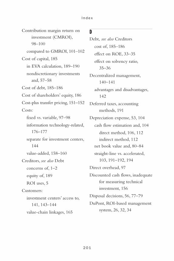
2 0 1
I n d e x
Contribution margin return on
investment (CMROI),
98–100
compared to GMROI, 101–102
Cost of capital, 185
in EVA calculation, 189–190
nondiscretionary investments
and, 57–58
Cost of debt, 185–186
Cost of shareholders’ equity, 186
Cost-plus transfer pricing, 151–152
Costs:
fixed vs. variable, 97–98
information technology-related,
176–177
separate for investment centers,
144
value-added, 158–160
Creditors, see also Debt
concerns of, 1–2
equity of, 189
ROI uses, 5
Customers:
investment centers’ access to,
141, 143–144
value-chain linkages, 165
DDebt, see also Creditors
cost of, 185–186
effect on ROE, 33–35
effect on solvency ratio,
35–36
Decentralized management,
140–141
advantages and disadvantages,
142
Deferred taxes, accounting
methods, 191
Depreciation expense, 53, 104
cash flow estimation and, 104
direct method, 106, 112
indirect method, 112
net book value and, 80–84
straight-line vs. accelerated,
103, 191–192, 194
Direct overhead, 97
Discounted cash flows, inadequate
for measuring technical
investment, 156
Disposal decisions, 56, 77–79
DuPont, ROI-based management
system, 26, 32, 34

EEarnings, see also Profit margin
projecting future, 5
quality of, 102–103
Economic performance
evaluation, 59–60
Economic value, 77, 85–87
Economic value added (EVA),
184, 188–195
accounting methods and,
188–192
calculation, 189
managed earnings and,
192–194
Efficiency variance, 128
Employees:
accounting for training of, 190
variance analysis and, 132
Equity:
cost of shareholders’, 186, 189
defined as property rights,
32–33, 189
Estimator, of ROI, 166–168, 169
Expenses:
defined, 190
managed earnings and,
192–194
FFIFO, see Inventory
Financial leverage, see Solvency
ratio
Fixed costs, 97
allocation issues, 134–136
CMROI and, 101–102
special purpose ratios and, 36
variances in, 130–137
Ford Motor Company, 12,
16–17, 27
balance sheet, 22–27
income statement, 18–21
ratio calculations, 27
segmented ROI analysis,
20–21, 26
segments disclosure, 28–32, 60,
62–67
solvency ratio and, 37–38
Fraud, 53
Full-cost transfer pricing,
150–151
GGross book value, 77–80
disposal decisions, 56, 77–79
replacement decisions, 54–57,
79–80
2 0 2
E S S E N T I A L S o f C o r p o r a t e P e r f o r m a n c e M e a s u r e m e n t

Gross margin, 90–91
Gross margin return on invest-
ment (GMROI), 89–90, 112
calculation, 90
compared to CMROI,
101–102
compared to ROI, 90–91
components of, 91–92
improving of, 92
with gross margin, 93
with increased turnover,
94–95
with markup, 96
including markup in, 96
HHertz, see Ford, segmented ROI
analysis
Historical cost:
accounting methods, 190–191
price-level adjusted, 85
Hurdle rate, 58, 184
IIncome statement, basic structure
of, 92. See also specific
companies
Incremental (increased) costs, 98
Incremental (increased) fixed
costs, 97
Information technology, see
Technology investment
Infrastructure technology, 157,
165–180
benefits component, 176
cost component, 176–177
guidelines/estimates for,
166–169
investment component, 175
metrics of, 170–175
payback, 177–178
productivity increases, 179–180
value of ROIT analysis,
168–170
Intangible costs, 176–177
Interest expense, profit
measurement and, 60–61
Internal rate of return, inadequate
for measuring technical
investment, 156
Inventory, see also Asset/
investment turnover
cost fluctuations and, 49–50
EVA and, 192–193, 195
LIFO vs. FIFO, 193
reducing investment in, 94–95
2 0 3
I n d e x
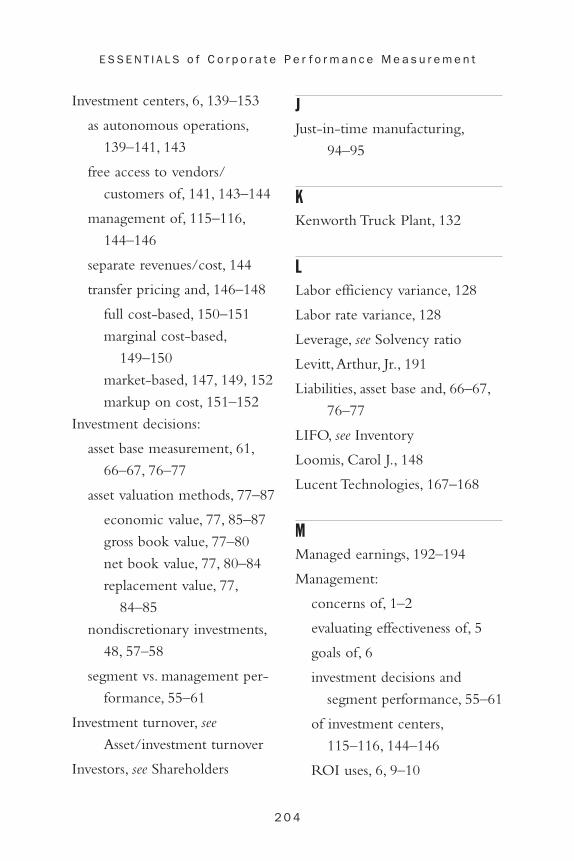
Investment centers, 6, 139–153
as autonomous operations,
139–141, 143
free access to vendors/
customers of, 141, 143–144
management of, 115–116,
144–146
separate revenues/cost, 144
transfer pricing and, 146–148
full cost-based, 150–151
marginal cost-based,
149–150
market-based, 147, 149, 152
markup on cost, 151–152
Investment decisions:
asset base measurement, 61,
66–67, 76–77
asset valuation methods, 77–87
economic value, 77, 85–87
gross book value, 77–80
net book value, 77, 80–84
replacement value, 77,
84–85
nondiscretionary investments,
48, 57–58
segment vs. management per-
formance, 55–61
Investment turnover, see
Asset/investment turnover
Investors, see Shareholders
JJust-in-time manufacturing,
94–95
KKenworth Truck Plant, 132
LLabor efficiency variance, 128
Labor rate variance, 128
Leverage, see Solvency ratio
Levitt,Arthur, Jr., 191
Liabilities, asset base and, 66–67,
76–77
LIFO, see Inventory
Loomis, Carol J., 148
Lucent Technologies, 167–168
MManaged earnings, 192–194
Management:
concerns of, 1–2
evaluating effectiveness of, 5
goals of, 6
investment decisions and
segment performance, 55–61
of investment centers,
115–116, 144–146
ROI uses, 6, 9–10
2 0 4
E S S E N T I A L S o f C o r p o r a t e P e r f o r m a n c e M e a s u r e m e n t
Manufacturing contribution
margin, 98–99
Manufacturing cost components,
93
Margin, see Profit margin
Marginal cost, 98
transfer pricing based on,
149–150
Market-based transfer pricing,
147, 149, 152
Market share variance analysis,
118–119
Market size variance analysis,
116–117
Market value added (MVA),
194–195
Markup:
in CMROI, 101
including in GMROI, 96
on costs, 151–152
Materials usage variance, 128
META Group Consulting, 178
Minimum rate of return, 184
determining, 185–187
NNet book value, 77, 80–84
Net income, 12, 91
Net operating profit after taxes
(NOPAT), 189–190
Net present value (NPV), 59
inadequate for measuring
technical investment, 156
Nondiscretionary investments, 48,
57–58
Nonvalue-added costs, 158–160
OOperating control, required for
investment centers, 139–141
Operating income, 12
Operations technology investment
analysis, 156–165
value-added cost approach,
158–160
value chain approach, 157,
160–165
Owners:
concerns of, 1–2
equity of, 37
ROI uses, 5
PPayback, 177–178
Planning, see Budgets
Price-level adjusted historical
cost, 85
2 0 5
I n d e x
Price variance, 127–128
calculating, 129
causes of, 128, 130
Productivity, increases in,
179–180
Profitability, see Profit margin
Profit center manager,
115–116
Profit margin, see also Economic
value added (EVA)
asset turnover and, 9–12, 53
calculating, 2–3, 10
in CMROI, 100–101
DuPont system, 26, 32, 34
gearing with ROI, 47–53
goals increased when
delegated, 1, 7
measuring, 60–61
of Coca-Cola/Ford, 12, 16–17,
27, 36–37
transfer prices and, 150
Property rights, equity defined as,
32–33, 189
QQuality of earnings, 102–103
Quantity variance, 127
calculating, 129
causes of, 128, 130
RRate of return, 5
Rate variances, 128
Replacement decisions, 54–57,
79–80
Replacement value, 77, 84–85
Research and development,
accounting methods, 190
Reserves, accounting methods,
191
Residual income (RI), 59,
184–188
minimum rate of return and,
184–187
return on investment, 187–188
targeted, 185
Return on equity (ROE), 32–33
effect of debt on, 33–35
shareholders and, 53–54
solvency ratio and, 36–37
Return on information
technology (ROIT), see
Technology investment
Return on investment (ROI):
2 0 6
E S S E N T I A L S o f C o r p o r a t e P e r f o r m a n c e M e a s u r e m e n t

advantages, 4–7, 39, 46–48
calculation, 4
defined, 3–5
disadvantages, 183–184
drawbacks of targeted, 47–53
GMROI compared to, 90–91
uses, 5–6
Return on technology investment
(ROTI), see Technology
investment
Revenue, 102–103
managed earnings and,
115–116, 192–194
separate for investment centers,
144
SSales:
accounting methods, 190
cash return on, 103–104
collection variance analysis,
122–123
price variance analysis, 121–122
volume variance analysis,
119–120
“Sandy Weill’s Monster”
(Loomis), 148
Segment analysis:
DuPont, 26, 32, 34
Ford, 20–21, 26
Ford’s disclosures, 28–32, 60,
62–67
investment decisions and
management performance,
55–61
with ROI, 39, 46–51
with ROI, drawbacks, 47–53
Service centers, 145–146
Shareholders:
cost of equity, 186, 189
ROE and, 32–33, 53–54
Solvency ratio, 35
effect of debt on, 35–36
effect on ROE, 37–39
ROE and, 36–37
Spending variance, 128
Stakeholders, see Shareholders
Standard cost, 125
Standards, setting, 137
Stern Stewart & Co., 184
Straight-line depreciation,
53, 103
vs. accelerated, 103, 191–192,
194
2 0 7
I n d e x
Summary variance analysis,
123–124
Suppliers, seeVendors
TTargeted residual income, 185
Targeted ROI:
drawbacks, 51–53
investment decisions and, 59
Technology investment, 155–181
infrastructure technology, 157,
165–180
benefits component, 176
cost component, 176–177
guidelines/estimates for,
166–169
investment component, 175
metrics of, 170–175
payback, 177–178
productivity increases,
179–180
value of ROIT analysis,
168–170
intangible benefits of,
155–156, 168–170
operations technology,
156–165
value-added cost approach,
158–160
value chain approach, 157,
160–165
Transfer pricing, 146–148
full cost-based, 150–151
marginal cost-based, 149–150
market-based, 147, 149, 152
markup on cost, 151–152
Turnover, see Asset/investment
turnover
UUsage variances, 128
VValuation, see Asset valuation
methods
Value-added costs, 158–160
Value chain approach, to
technology investment
analysis, 160–165
external, 164–165
internal, 162–163
Variable costs, 97–98
in CMROI, 98, 101
three-component, 100–101
two-component, 100
variance analysis
budgeted costs, 126–128
cost standards, 125–130
Variance analysis:
employee participation in, 132
fixed costs, 130–137
2 0 8
E S S E N T I A L S o f C o r p o r a t e P e r f o r m a n c e M e a s u r e m e n t

2 0 9
I n d e x
market share, 118–119
market size, 116–117
sales collection, 122–123
sales price, 121–122
sales volume, 119–120
summary variance analysis,
123–124
variable costs, 125–130
budget costs, 126–128
causes of, 128–130
cost standards, 125
Vendors:
investment centers’ access to,
141, 143–144
ROI estimators of, 166–169
value-chain linkages, 164–165
WWal-Mart Stores:
financial data, 40–41
ROI/ROE of, 38–39
Weighted average cost of capital
(WACC), 186
calculating, 186–187
Weill, Sanford, 148