Essential Partial Differential Equations Examples 1

The exercises marked with ? are the most important.

(1.1) Check that the examples of explicit solutions to Poisson, wave heat and Laplacegiven in Lecture 1 are indeed solutions to the problems.

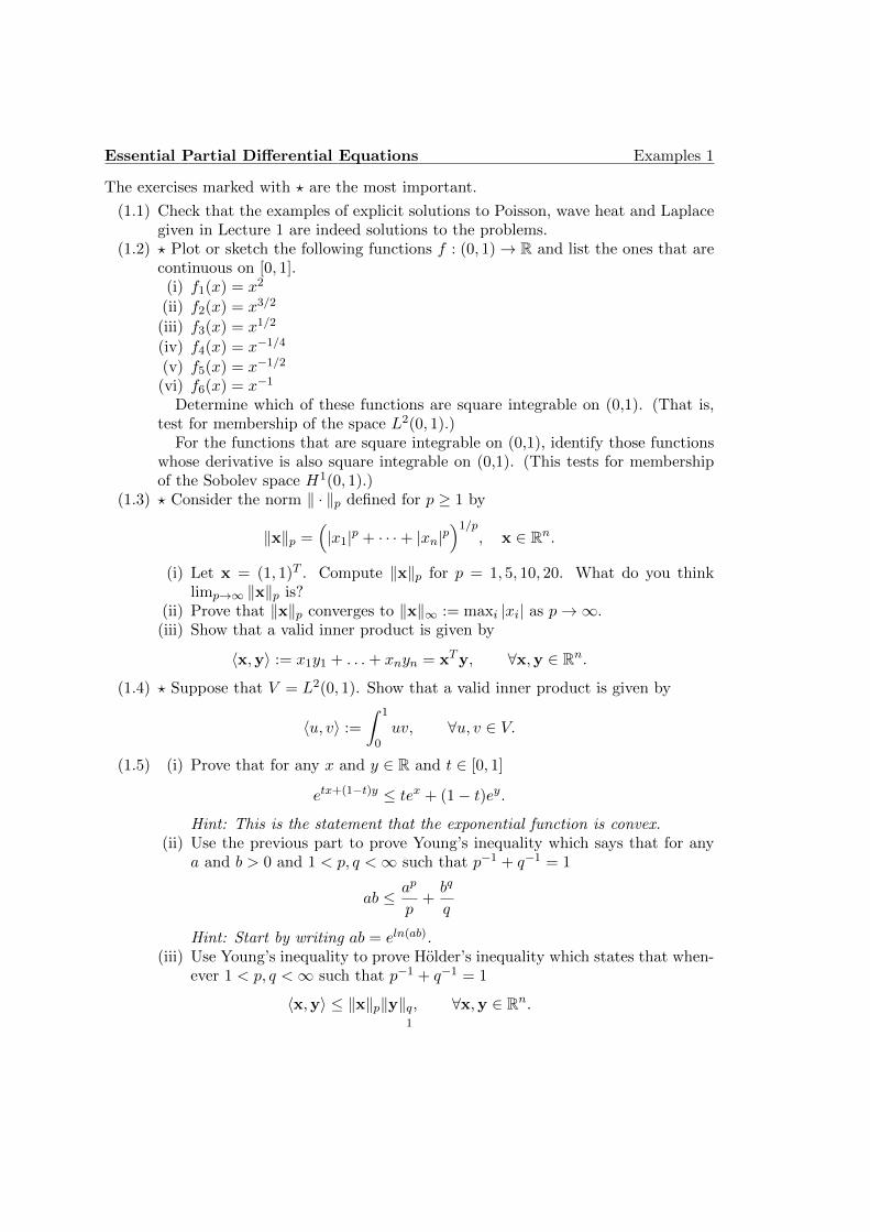
(1.2) ? Plot or sketch the following functions f : (0, 1)→ R and list the ones that arecontinuous on [0, 1].

(i) f1(x) = x2

(ii) f2(x) = x3/2

(iii) f3(x) = x1/2

(iv) f4(x) = x−1/4

(v) f5(x) = x−1/2

(vi) f6(x) = x−1

Determine which of these functions are square integrable on (0,1). (That is,test for membership of the space L2(0, 1).)

For the functions that are square integrable on (0,1), identify those functionswhose derivative is also square integrable on (0,1). (This tests for membershipof the Sobolev space H1(0, 1).)

(1.3) ? Consider the norm ‖ · ‖p defined for p ≥ 1 by

‖x‖p =(|x1|p + · · ·+ |xn|p

)1/p, x ∈ Rn.

(i) Let x = (1, 1)T . Compute ‖x‖p for p = 1, 5, 10, 20. What do you thinklimp→∞ ‖x‖p is?

(ii) Prove that ‖x‖p converges to ‖x‖∞ := maxi |xi| as p→∞.(iii) Show that a valid inner product is given by

〈x,y〉 := x1y1 + . . .+ xnyn = xTy, ∀x,y ∈ Rn.

(1.4) ? Suppose that V = L2(0, 1). Show that a valid inner product is given by

〈u, v〉 :=

∫ 1

0uv, ∀u, v ∈ V.

(1.5) (i) Prove that for any x and y ∈ R and t ∈ [0, 1]

etx+(1−t)y ≤ tex + (1− t)ey.

Hint: This is the statement that the exponential function is convex.(ii) Use the previous part to prove Young’s inequality which says that for any

a and b > 0 and 1 < p, q <∞ such that p−1 + q−1 = 1

ab ≤ ap

p+bq

q

Hint: Start by writing ab = eln(ab).(iii) Use Young’s inequality to prove Holder’s inequality which states that when-

ever 1 < p, q <∞ such that p−1 + q−1 = 1

〈x,y〉 ≤ ‖x‖p‖y‖q, ∀x,y ∈ Rn.1

2

Here the inner product and norms were defined in exercise 1.3. Hint: Con-sider proving ⟨

x

‖x‖p,

y

‖y‖q

⟩≤ 1

which is equivalent.Note that essentially the same proof applies in the case of integrals and theL2 inner product to show that when 1 < p, q <∞ are such that p−1+q−1 = 1∫ b

au(t)v(t) dt ≤

(∫ b

a|u(t)|p dt

)1/p(∫ b

a|v(t)|q dt

)1/q

.

(1.6) Let X be a Banach space. Then the set of linear operators A : X → X is itselfa vector space. Such a linear operator is called bounded if

‖A‖ = supx 6=0

‖Ax‖‖x‖

<∞.

(i) Show that ‖ · ‖ so defined is a valid norm on the set L(X) of bounded linearoperators mapping X to itself.

(ii) Show further that an equivalent definition for ‖A‖ is given by

‖A‖ = infM ∈ R : ‖Ax‖ ≤M‖x‖,∀x ∈ X.(iii) Show that if A and B : X → X are both bounded linear operators on X

then the composition AB is also a bounded linear operator on X. Provethat

‖AB‖ ≤ ‖A‖‖B‖.

3

Essential Partial Differential Equations Solutions 1

(1.1) Just follows directly from differentiation.(1.2) The six functions f1, f2, . . . , f6 are plotted below. The functions with positive

exponents are continuous over [0, 1]. The functions with negative exponent areunbounded in the limit x→ 0 so are not continuous.

0 0.1 0.2 0.3 0.4 0.5 0.6 0.7 0.8 0.9 10

0.5

1

1.5

2

2.5

3

x

f(x)

x2

x3/2

x1/2

x−1/4

x−1/2

x−1

To determine square integrability we need to check each function in turn to

see if∫ 1

0 f2i < ∞. The results are tabulated below. It is easy to see that all

functions xα with α > −1/2 are in L2(0, 1).

fi fi ∈ L2(0, 1) f ′i ∈ L2(0, 1)x2 X X

x32 X X

x12 X ×

x−14 X ×

x−12 × ×

x−1 × ×

We can similarly check the square integrability of f ′i . In this case we see thatxα has a derivative L2(0, 1) in the case α > 1/2. Thus continuous functions neednot have square integrable first derivatives!

(1.3) (i) ‖x‖p = 21/p. Thus, limp→∞ ‖x‖p = 1.

4

(ii) To prove that ‖x‖p → ‖x‖∞ as p → ∞, We let x have maximum value inits first component so that ‖x‖∞ = |x1|. Then

‖x‖p = |x1|( n∑

i=1

(|xi|/|x1|)p)1/p

.

Notice all the terms in the sum are less than 1 and hence ‖x‖p ≤ |x1|n1/p →|x1| as p→∞. Finally, since it is clear that ‖x‖p ≥ |x1|, the result follows.

(iii) To show that 〈·, ·〉 is a valid inner product we need to check the axioms:• symmetry

〈x,y〉 = x1y1 + . . .+ xnyn = y1x1 + . . .+ ynxn = 〈y,x〉 ♥• positivity

〈x,x〉 = x21︸︷︷︸≥0

+ . . .+ x2n︸︷︷︸≥0

≥ 0 ♥

• uniqueness

〈x,x〉 = 0 ⇐⇒ x21︸︷︷︸≥0

+ . . .+ x2n︸︷︷︸≥0

= 0 ⇐⇒ xi = 0, ∀i. ♥

• linearity

〈αx + βy,w〉 = (αx1 + βy1)w1 + . . .+ (αxn + βyn)wn

= αx1w1 + βy1w1 + . . .+ αxnwn + βynwn

= α(x1w1 + . . .+ xnwn) + β(y1w1 + . . .+ ynwn)

= α〈x,w〉+ β〈y,w〉 ♥(1.4) Checking the inner product axioms:

• symmetry

(u, v) =

∫ 1

0uv =

∫ 1

0vu = (v, u) ♥

• positivity

(u, u) =

∫ 1

0u2︸︷︷︸≥0

≥ 0 ♥

• uniqueness

(u, u) = 0 ⇐⇒∫ 1

0u2︸︷︷︸≥0

= 0 ⇐⇒ u = 0 almost everywere. ♥

• linearity

(αu+ βv,w) =

∫ 1

0αu+ βvw = α

∫ 1

0uw + β

∫ 1

0vw = α(u,w) + β(v, w) ♥

(1.5) (i) Set f(t) = etx+(1−t)y − tex − (1 − t)ey. The problem then is to prove thatf(t) ≤ 0 for t ∈ (0, 1). Note that

f ′′(t) = (x− y)2etx+(1−t)y ≥ 0,

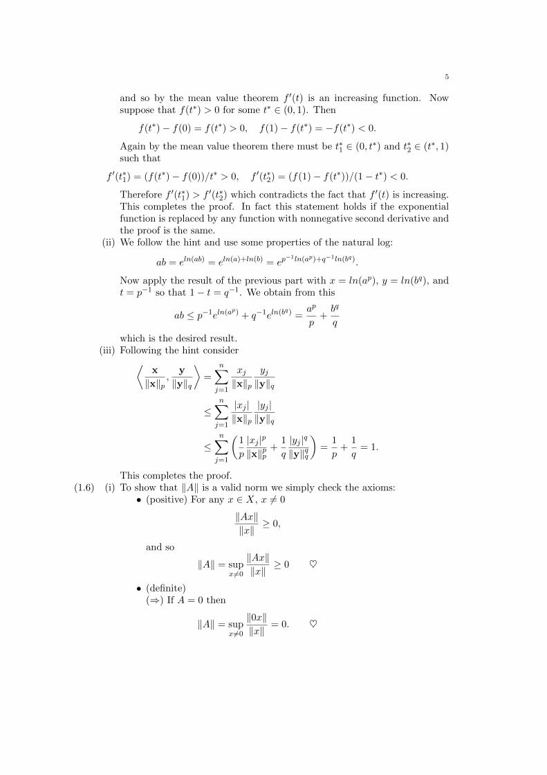
5

and so by the mean value theorem f ′(t) is an increasing function. Nowsuppose that f(t∗) > 0 for some t∗ ∈ (0, 1). Then

f(t∗)− f(0) = f(t∗) > 0, f(1)− f(t∗) = −f(t∗) < 0.

Again by the mean value theorem there must be t∗1 ∈ (0, t∗) and t∗2 ∈ (t∗, 1)such that

f ′(t∗1) = (f(t∗)− f(0))/t∗ > 0, f ′(t∗2) = (f(1)− f(t∗))/(1− t∗) < 0.

Therefore f ′(t∗1) > f ′(t∗2) which contradicts the fact that f ′(t) is increasing.This completes the proof. In fact this statement holds if the exponentialfunction is replaced by any function with nonnegative second derivative andthe proof is the same.

(ii) We follow the hint and use some properties of the natural log:

ab = eln(ab) = eln(a)+ln(b) = ep−1ln(ap)+q−1ln(bq).

Now apply the result of the previous part with x = ln(ap), y = ln(bq), andt = p−1 so that 1− t = q−1. We obtain from this

ab ≤ p−1eln(ap) + q−1eln(bq) =ap

p+bq

q

which is the desired result.(iii) Following the hint consider⟨

x

‖x‖p,

y

‖y‖q

⟩=

n∑j=1

xj‖x‖p

yj‖y‖q

≤n∑j=1

|xj |‖x‖p

|yj |‖y‖q

≤n∑j=1

(1

p

|xj |p

‖x‖pp+

1

q

|yj |q

‖y‖qq

)=

1

p+

1

q= 1.

This completes the proof.(1.6) (i) To show that ‖A‖ is a valid norm we simply check the axioms:

• (positive) For any x ∈ X, x 6= 0

‖Ax‖‖x‖

≥ 0,

and so

‖A‖ = supx 6=0

‖Ax‖‖x‖

≥ 0 ♥

• (definite)(⇒) If A = 0 then

‖A‖ = supx 6=0

‖0x‖‖x‖

= 0. ♥

6

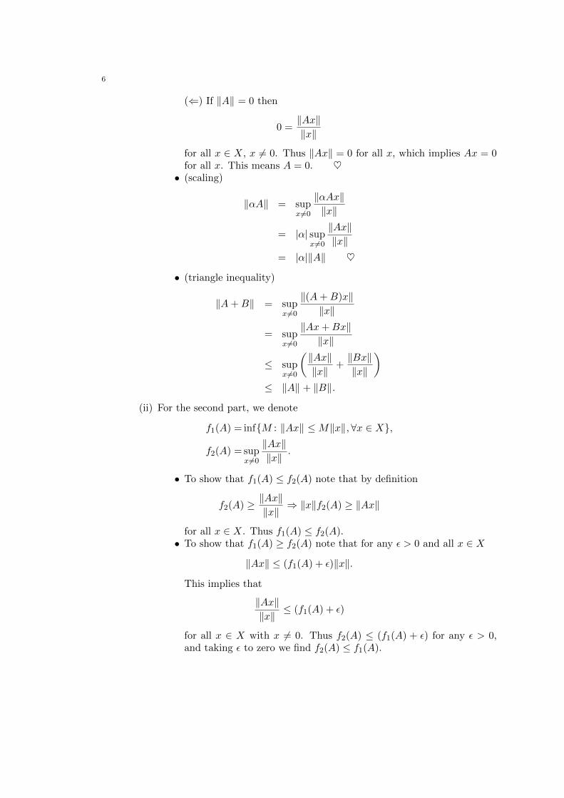
(⇐) If ‖A‖ = 0 then

0 =‖Ax‖‖x‖

for all x ∈ X, x 6= 0. Thus ‖Ax‖ = 0 for all x, which implies Ax = 0for all x. This means A = 0. ♥• (scaling)

‖αA‖ = supx 6=0

‖αAx‖‖x‖

= |α| supx6=0

‖Ax‖‖x‖

= |α|‖A‖ ♥

• (triangle inequality)

‖A+B‖ = supx6=0

‖(A+B)x‖‖x‖

= supx 6=0

‖Ax+Bx‖‖x‖

≤ supx 6=0

(‖Ax‖‖x‖

+‖Bx‖‖x‖

)≤ ‖A‖ + ‖B‖.

(ii) For the second part, we denote

f1(A) = infM : ‖Ax‖ ≤M‖x‖, ∀x ∈ X,

f2(A) = supx 6=0

‖Ax‖‖x‖

.

• To show that f1(A) ≤ f2(A) note that by definition

f2(A) ≥ ‖Ax‖‖x‖

⇒ ‖x‖f2(A) ≥ ‖Ax‖

for all x ∈ X. Thus f1(A) ≤ f2(A).• To show that f1(A) ≥ f2(A) note that for any ε > 0 and all x ∈ X

‖Ax‖ ≤ (f1(A) + ε)‖x‖.

This implies that

‖Ax‖‖x‖

≤ (f1(A) + ε)

for all x ∈ X with x 6= 0. Thus f2(A) ≤ (f1(A) + ε) for any ε > 0,and taking ε to zero we find f2(A) ≤ f1(A).

7

(iii) For the last part we have

‖AB‖ = supx 6=0

‖ABx‖‖x‖

≤ supx 6=0

‖A‖‖Bx‖‖x‖

(Part (ii))

≤ ‖A‖‖B‖ (Definition of ‖B‖).

8

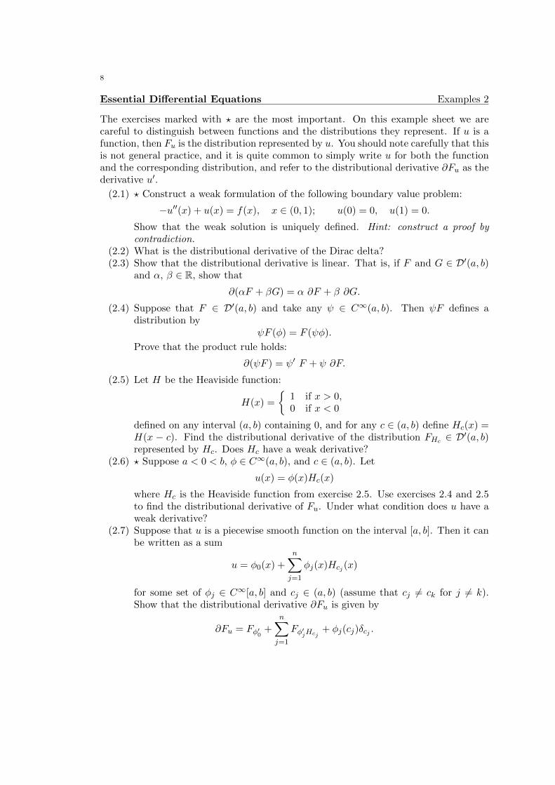
Essential Differential Equations Examples 2

The exercises marked with ? are the most important. On this example sheet we arecareful to distinguish between functions and the distributions they represent. If u is afunction, then Fu is the distribution represented by u. You should note carefully that thisis not general practice, and it is quite common to simply write u for both the functionand the corresponding distribution, and refer to the distributional derivative ∂Fu as thederivative u′.

(2.1) ? Construct a weak formulation of the following boundary value problem:

−u′′(x) + u(x) = f(x), x ∈ (0, 1); u(0) = 0, u(1) = 0.

Show that the weak solution is uniquely defined. Hint: construct a proof bycontradiction.

(2.2) What is the distributional derivative of the Dirac delta?(2.3) Show that the distributional derivative is linear. That is, if F and G ∈ D′(a, b)

and α, β ∈ R, show that

∂(αF + βG) = α ∂F + β ∂G.

(2.4) Suppose that F ∈ D′(a, b) and take any ψ ∈ C∞(a, b). Then ψF defines adistribution by

ψF (φ) = F (ψφ).

Prove that the product rule holds:

∂(ψF ) = ψ′ F + ψ ∂F.

(2.5) Let H be the Heaviside function:

H(x) =

1 if x > 0,0 if x < 0

defined on any interval (a, b) containing 0, and for any c ∈ (a, b) define Hc(x) =H(x − c). Find the distributional derivative of the distribution FHc ∈ D′(a, b)represented by Hc. Does Hc have a weak derivative?

(2.6) ? Suppose a < 0 < b, φ ∈ C∞(a, b), and c ∈ (a, b). Let

u(x) = φ(x)Hc(x)

where Hc is the Heaviside function from exercise 2.5. Use exercises 2.4 and 2.5to find the distributional derivative of Fu. Under what condition does u have aweak derivative?

(2.7) Suppose that u is a piecewise smooth function on the interval [a, b]. Then it canbe written as a sum

u = φ0(x) +n∑j=1

φj(x)Hcj (x)

for some set of φj ∈ C∞[a, b] and cj ∈ (a, b) (assume that cj 6= ck for j 6= k).Show that the distributional derivative ∂Fu is given by

∂Fu = Fφ′0 +

n∑j=1

Fφ′jHcj+ φj(cj)δcj .

9

Under what condition will u have a weak derivative?(2.8) ? Consider the following piecewise continuous functions h : (−1, 1)→ R:

h1(x) =

−1, −1 < x < 0;

1, 0 < x < 1.

h2(x) =

−x, −1 < x < 0;

x, 0 < x < 1.

Show that both functions are in L2(−1, 1). What are the distributional deriva-tives ∂Fh1 and ∂Fh2? Is either function in the Sobolev space H1(−1, 1)?

10

‘ Essential Partial Differential Equations Solutions 2

(2.1) We consider the problem

−u′′ + u = f, u(0) = u(1) = 0.

Multiplying by a test function v ∈ H10 (0, 1) and integrating by parts gives

−∫ 1

0u′′v dx+

∫ 1

0uv dx =

∫ 1

0fv dx

−[u′v]1

0+

∫ 1

0u′(x)v′(x) dx+

∫ 1

0u(x)v(x) dx =

∫ 1

0f(x)v(x) dx.

The first term is zero because v ∈ H10 (0, 1) means that v(0) = v(1) = 0. Denot-

ing the standard L2(0, 1) inner product and associated norm by (·, ·) and ‖ · ‖,respectively, the weak formulation is:

Given F ∈ H10 (0, 1)∗, find u ∈ H1

0 (0, 1) such that

(u′, v′) + (u, v) = F (v)

for all test functions v ∈ H10 (0, 1).

Using the notation A(u, v) = (u′, v′) + (u, v), the formula in the weak formu-lation can be written in the simpler form

A(u, v) = F (v).

A is a bilinear function on H10 (0, 1). Moreover, since it is symmetric, and since

A(u, u) = ‖u′‖2 + ‖u‖2 ≥ 0 with

A(u, u) = 0 ⇐⇒ ‖u′‖2︸ ︷︷ ︸≥0

+ ‖u‖2︸︷︷︸≥0

= 0

⇐⇒ ‖u‖ = 0

⇐⇒ u = 0 a.e. in (0,1)

we find that A defines an inner product on H10 (0, 1).

To show uniqueness of solution, we suppose that u1, u2 ∈ H10 (0, 1) are both

weak solutions and let e = u1 − u2. Then

A(u1, v)−A(u2, v) = A(e, v) = F (v)− F (v) = 0,

for any v ∈ H10 (0, 1). Putting v = e we find that A(e, e) = 0 and hence we have

that u1 = u2 a.e. in (0, 1).(2.2) The distributional derivative of the Dirac delta is defined by

∂δ(φ) = −δ(φ′) (definition of distributional derivative)

= −φ′(0) (definition of Dirac delta).

Thus ∂δ is the distribution which maps a function φ to φ′(0).

11

(2.3) This follows from the definition of the distributional derivative. For any ϕ ∈C∞0 (a, b)

∂(αF + βG)(ϕ) = −(αF + βG)(ϕ′) (definition of distributional derivative)

= −αF (ϕ′)− βG(ϕ′) (addition of functionals)

= −F (αϕ′)−G(βϕ′) (property of linear functionals)

= ∂F (αϕ) + ∂G(βϕ) (definition of distributional derivative)

= α ∂F (ϕ) + β ∂G(ϕ) (property of linear functionals)

= (α ∂F + β ∂G)(ϕ) (addition of linear functionals).

(2.4) This follows from the definition of the distributional derivative and the classicalproduct rule. For any ϕ ∈ C∞0 (a, b)

∂(ψF )(ϕ) = −ψF (ϕ′) (definition of distributional derivative)

= −F (ψϕ′) (definition of ψF )

= −F ((ψϕ)′ − ψ′ϕ) (Classical product rule)

= −F ((ψϕ)′) + F (ψ′ϕ) (property of linear functional)

= ∂F (ψϕ) + F (ψ′ϕ) (definition of distributional derivative)

= ψ∂F (ϕ) + ψ′F (ϕ) (definition of ψF ).

(2.5) To calculate the distributional derivative of FHc we start from the definition ofdistributional derivative. For any ϕ ∈ C∞0 (a, b):

∂FHc(ϕ) = −FHc(ϕ′) (definition of distributional derivative)

= −∫ b

aH(x− c)ϕ′ dx (definition of FHc)

= −∫ b

cϕ′(x) dx (definition of H)

= −ϕ(b) + ϕ(c) (Fundamental Theorem of Calculus)

= ϕ(c) (since ϕ(b) = 0)

= δc(ϕ) (definition of Dirac delta)

Therefore ∂FHc = δc. Since the Dirac delta δc is not represented by any functionH does not have a weak derivative.

(2.6) Here we can apply the product rule for distributions and the distributional de-rivative of FHc found in the previous exercise.

∂Fu = ∂(FφHc) (definition of u)

= ∂(φFHc) (follows from definition of φFHc)

= φ∂FHc + φ′FHc (product rule from exercise 2.4)

= φδc + φ′FHc (exercise 2.5)

= φ(c)δc + φ′FHc (follows from definition of Dirac delta).

12

Thus∂Fu = φ(c)δc + Fφ′Hc .

This distribution is represented by a function if and only if φ(c) = 0, and so uhas a weak derivative if and only if φ(c) = 0. In that case the weak derivative ofu is φ′Hc. Note the condition that φ(c) = 0 is equivalent to the condition that uis continuous.

(2.7) The formula follows easily from all of the previous exercises. As in exercise 6 wealso see that ∂Fu is represented by the function

φ′0 +∑j

φ′jHcj

when φj(cj) = 0 for all j. This formula therefore gives the weak derivative of uin this case. Furthermore, the condition φj(cj) = 0 for all j is equivalent to thecondition that u is continuous.

The consequence of this exercise is that when we have a continuous functionthat is piecewise differentiable in the classical sense with bounded derivatives,then the weak derivative exists and is found simply by taking the derivative oneach interval where the function is classically differentiable. If the function alsohas jumps (i.e. it is not continuous) then there are also Dirac deltas in thedistributional derivative and so there is no weak derivative. The coefficient ofthe Dirac delta at cj corresponds with φj(cj) which is exactly the size of thejump in the function u at cj .

(2.8) A simple calculation shows that h1 and h2 are both square integrable; e.g.∫ 1−1 h

21 =

∫ 0−1(−1)2 +

∫ 10 (1)2 = 2 < ∞. The distributional derivatives of h1 and

h2 can be found from the previous exercises (although for h2 see also example??) using

h2(x) = −x+ 2xH(x), h1(x) = −1 + 2H(x).

By exercise 6

∂Fh2 = F−1 + 2FH = F−1+2H , ∂Fh1 = 2δ.

Thus h1 is the weak derivative of h2 (which agrees with example ??), and h1

does not have a weak derivative. Therefore h2 ∈ H1(−1, 1), but h1 /∈ H1(−1, 1).

13

Essential Differential Equations Examples 3

The exercises marked with a ? are the most important.

(3.1) Consider the following weak problem: Find u ∈ H10 (0, 1) such that∫ 1

0u′(x)v′(x)dx =

∫ 1/2

0v(x) dx, ∀v ∈ H1

0 (0, 1).

Solve this problem. Hint: It may be useful to first consider the classical ODEproblem corresponding to this weak problem.

(3.2) Suppose that f(x) is a function on [0, 1] which is piecewise continuous. In par-ticular, suppose that

0 = a0 < a1 < ... < an−1 < an = 1

is a partition of the interval [0, 1], and that f is a continuous function whenrestricted to each interval (aj , aj+1) for j = 0 to n − 1. Consider the weakproblem: Find u ∈ H1

0 (0, 1) such that∫ 1

0u′(x)v′(x)dx =

∫ 1

0f(x)v(x) dx, ∀v ∈ H1

0 (0, 1).

Show that the unique solution u of this problem satisfies the following conditions.(i) u′ is continuous.

(ii) Restricted to each interval (aj , aj+1) u′ is classically differentiable and sat-isfies

−u′′(x) = f(x) ∀x ∈ (aj , aj+1).

Combined with the requirements that u is continuous and u(0) = u(1) = 0(which hold because u ∈ H1

0 (0, 1)) this is enough to solve uniquely for u, andgives us a method to solve weak problems when the right hand side is a piecewisecontinuous function.

(3.3) Suppose that u ∈ H20 (0, 1). Show that∫ 1

0u′(x)2 dx ≤

∫ 1

0u′′(x)2 dx.

(3.4) ? Given c ∈ (0, 1), show that there is a constant C > 0 such that

|u(c)| ≤ C‖u‖H1(0,1)

for all u ∈ C1[0, 1]. This can be used to prove that the Dirac delta δc is a boundedlinear functional on H1(0, 1) as claimed in lecture and the notes.

(3.5) ? Construct the weak formulation for the problem

−u′′(x) = f(x), x ∈ (0, 1); u(0) = 0, u′(1) = 1.

Find the solution of the weak formulation in each of the following cases.(i) F = δ1/2.

(ii) F = H1/2 where H1/2 is the Heaviside function (see exercise 2.5). Notethat technically in the weak formulation F should be the linear functionalrepresented by H1/2, but here we do not distinguish between the functionand the corresponding functional.

14

(3.6) Let Ω be a connected and bounded domain in R2 or R3, with smooth boundary∂Ω made up of distinct parts ∂ΩD and ∂ΩN . Given that f ∈ L2(Ω), construct aweak formulation of the PDE problem

−∇ · ∇u(~x) = f(~x), ~x ∈ Ω,

subject to the boundary conditions,

u= 0 on ∂ΩD and∂u

∂n:= ∇u · ~n= 0 on ∂ΩN ,

where ~n is the outward pointing normal vector. The solution space and the testspace should be identical by construction. Also prove that the weak solutionmust be unique. Hint: follow the construction used in the one-dimensional case.Use the vector identity

∇ · (v∇u) = v∇ · ∇u+∇v · ∇uand apply the divergence theorem.

(3.7) ? Let A be an n× n matrix which is symmetric positive definite. This means

A = AT (symmetric)

andxTAx > 0 ∀x ∈ Rn, x 6= 0 (positive definite).

(i) Show that a valid inner product on Rn is given by

(x,y)A = xTAy.

(ii) Let H = (Rn, (·, ·)A) be the finite dimensional Hilbert space made up of thevector space Rn and the inner product (·, ·)A. Suppose that f ∈ Rn andshow that the map F defined by

Rn 3 v 7→ fTv = F (v)

is a bounded linear functional on H.(iii) What is the Riesz representation of the bounded linear functional F on H

defined in part (b)?

15

Essential Partial Differential Equations Solutions 3

(3.1) Following the hint note that the corresponding ODE problem is

−u′′(x) = H1/2(x), u(0) = u(1) = 0.

For x ∈ (0, 1/2) we have u′′(x) = −1, and the general solution of this ODE is

u(x) = a1x+ a2 −x2

2

for unknown constants a1 and a2. Since we require u(0) = 0, we should havea2 = 0 and so

u(x) = a1x−x2

2for x ∈ [0, 1/2). Next, for x ∈ (1/2, 1] we have u′′(x) = 0 and the general solutionof this ODE is

u(x) = b1x+ b2.

We need to have u(1) = 0, and so b1 + b2 = 0. Thus

u(x) = b1(x− 1)

for x ∈ (1/2, 1]. So we guess that the solution should have the form

u(x) =

(a1x−

x2

2

)+

(b1(x− 1)− a1x+

x2

2

)H1/2(x).

To guarantee that u ∈ H10 (0, 1) we must make u continuous, and for this we need

b1((1/2)− 1)− a1(1/2) +(1/2)2

2= 0→ b1 =

1

4− a1.

This gives

u(x) =

(a1x−

x2

2

)+

(a1(1− 2x) +

1

4(x− 1) +

x2

2

)H1/2(x).

Since u is continuous, it has a weak derivative given by

u′(x) = a1 − x+

(x− 2a1 +

1

4

)H1/2(x).

Now let us put this into the formula for the weak problem which must hold forany v ∈ H1

0 (0, 1):∫ 1/2

0(a1 − x)v′(x) dx−

∫ 1

1/2

(a1 −

1

4

)v′(x) dx =

∫ 1/2

0v(x) dx.

Using integration by parts and the fundamental theorem of calculus on the lefthand side we get∫ 1/2

0(a1 − x)v′(x) dx−

∫ 1

1/2

(a1 −

1

4

)v′(x) dx =

(2a1 −

3

4

)v(1/2) +

∫ 1/2

0v(x) dx.

For u to be a weak solution we therefore must have

2a1 −3

4= 0⇒ a1 =

3

8

16

Thus the solution of the weak problem is

u(x) =

(3x

8− x2

2

)+

(1

8− x

2+x2

2

)H1/2(x).

This can also be written as

u(x) =

3x

8− x2

2for 0 ≤ x < 1/2

1

8(1− x) for 1/2 < x ≤ 1.

Note that this is the same problem as discussed in example 2.1 from lecture ??.(3.2) Suppose that u ∈ H1(0, 1) is a function satisfying the given requirements. Then

for any v ∈ C10 (0, 1) ⊂ H1

0 (0, 1)∫ 1

0u′(x)v′(x) dx =

n−1∑j=0

∫ aj+1

aj

u′(x)v′(x) dx.

Since u′ is classically differentiable and −u′′ = f restricted to each interval, wecan integrate by parts on each interval (note that integration by parts requiresboth functions to be classically differentiable meaning we cannot directly applyintegration by parts on all of [0, 1]) to obtain∫ 1

0u′(x)v′(x) dx =

n−1∑j=0

∫ aj+1

aj

f(x)v(x) dx+ u′(aj)v(aj)− u′(aj+1)v(aj+1)

=

∫ 1

0f(x)v(x) dx+

n−1∑j=0

u′(aj+1)v(aj+1)− u′(aj)v(aj)

=

∫ 1

0f(x)v(x) dx+ u′(1)v(1)− u′(0)v(0).

Since v(0) = v(1) = 0 this proves that u solves the weak problem.It only remains to show that a u satisfying these conditions must exist. By

a theorem you should have studied in MATH10222 on each interval (aj , aj+1),since f is continuous, there is a general solution

uj(x) = bjx+ cj + dj(x)

satisfying −u′′j (x) = f(x) on (aj , aj+1) where bj and cj are arbitrary constants

to be determined. Recall that dj is any particular solution for −d′′j (x) = f(x) on

(aj , aj+1). Our solution u can now be constructed from these general solutionson each individual interval by imposing the conditions of continuity of u and u′

as well as the boundary conditions u(0) = u(1) = 0. Indeed, suppose we take

u(x) = uj(x) = bjx+ cj + dj(x)

for x ∈ (aj , aj+1). There are then 2n unknown coefficients (the numbers bj andcj for j = 0 to n− 1) which must be determined. The boundary conditions are

c0 = −dj(0), bn−1 + cn−1 = −dn−1(1).

17

The condition that u must be continuous is

bjaj+1 + cj + dj(aj+1) = bj+1aj+1 + cj+1 + dj+1(aj+1)

for j = 0 to n− 2. The condition that u′ must be continuous is

bj + d′j(aj+1) = bj+1 + d′j+1(aj+1)

for j = 0 to n− 2. There are thus 2n equations for the 2n unknowns bj and cj ,and it is quite plausible that there will be a solution and it will be unique. Toprove there is a solution we rewrite as follows

aj+1(bj+1 − bj) + (cj+1 − cj) = dj(aj+1)− dj+1(aj+1),

bj+1 − bj = d′j(aj+1)− d′j+1(aj+1).

These imply that

cj+1 = cj + dj(aj+1)− dj+1(aj+1)− aj+1(d′j(aj+1)− d′j+1(aj+1)).

Thus we can start with the boundary condition c0 = −dj(0) and inductivelydetermine all of the cj ’s. After cn−1 is found in this way, bn−1 is found by theother boundary condition bn−1 = −cn−1 − dn−1(1). Finally, we can use

bj = bj+1 − d′j(aj+1)− d′j+1(aj+1)

to determine all of the bj ’s. Thus we have shown that there is a function satisfyingthe hypotheses given for u, and we know that it must then be the unique solutionto the weak problem.

(3.3) As u(0) = u(1) = 0, we know that there exists a ξ ∈ [0, 1] with u′(ξ) = 0 by themean value theorem. Then,

u′(x) = u′(ξ) +

∫ x

ξu′′(s) ds =

∫ x

ξu′′(s) ds

The rest of the proof is essentially the same as the proof of the Poincare–Friedrichinequality given in the lectures which we now go through. We square both sidesof the equality above and integrate to obtain∫ 1

0u′(x)2 dx =

∫ 1

0

(∫ x

ξu′′(s) ds

)2

dx

≤∫ 1

0‖1‖2L2(ξ,x)‖u

′′‖2L2(ξ,x) dx (Cauchy-Schwarz inequality)

≤ ‖u′′‖2L2(0,1)

∫ 1

0|ξ − x| dx (Evaluate L2 norm and ‖u′′‖L2(ξ,x) ≤ ‖u′′‖L2(0,1))

≤ ‖u′′‖2L2(0,1) (|ξ − x| ≤ 1)

≤∫ 1

0u′′(x)2 dx (Definition of L2 norm).

(3.4) For u ∈ C1[0, 1] we have

u(c) =

∫ c

0

1

c(xu)′(x) dx =

1

c

∫ c

0(u(x) + xu′(x))dx.

18

Using the Cauchy-Schwarz inequality this gives

|u(c)| ≤ 1

c

∫ c

0(|u(x)|+ x|u′(x)|)dx (Previous equation and triangle inequality)

≤ 1

c

(‖1‖L2(0,c)‖u‖L2(0,c) + ‖x‖L2(0,c)‖u′‖L2(0,c)

)(Cauchy-Schwarz)

≤ 1

c

(√c‖u‖L2(0,c) +

c3/2

√3‖u′‖L2(0,c)

)(Calculation of L2 norms)

≤ 1√c‖u‖H1(0,1). (‖v‖L2(0,c) + ‖v′‖L2(0,c) ≤ ‖v‖H1(0,1) for any v ∈ H1(0, 1))

Note that c−1/2 is not the ideal constant for this estimate.(3.5) Assume that u is a classical solution of the given boundary value problem. To

find the weak formulation we first multiply the ODE by a test function v andintegrate

−∫ 1

0u′′(x)v(x) dx =

∫ 1

0f(x)v(x) dx.

Next integrate by parts on the left hand side to obtain∫ 1

0u′(x)v′(x) dx− u′(1)v(1) + u′(0)v(0) =

∫ 1

0f(x)v(x) dx.

Now we apply the boundary condition u′(1) = 1, and note that in order to makethe other boundary term vanish we must require v(0) = 0. If v(0) = 0 we thushave ∫ 1

0u′(x)v′(x) dx =

∫ 1

0f(x)v(x) dx+ v(1).

The space for the test function v is therefore

H = v ∈ H1(0, 1) : v(0) = 0.The weak formulation is the following. Given F ∈ H∗, find u ∈ H such that∫ 1

0u′(x)v′(x) dx = F (v) + δ1(v)

for all v ∈ H (note that v(1) = δ1(v)).Now we find the weak solutions in the given cases.

(i) Let F = δ1/2. As in exercise 1 on this sheet we suppose that the weaksolution u should be a classical solution on the two intervals (0, 1/2) and(1/2, 1) where f = 0. Thus u(x) should have the form of the followingansatz

u(x) =

a1x+ b1 for x ∈ (0, 1/2)a2x+ b2 for x ∈ (1/2, 1).

For u ∈ H ⊂ H1(0, 1) the function u must be continuous and u(0) = 0.From the boundary condition u(0) = 0 we find that b1 = 0, and for u to becontinuous at x = 1/2 we must have

a1

2=a2

2+ b2. (1)

19

Finally, u must satisfy∫ 1

0u′(x)v′(x) dx = v(1/2) + v(1)

for any v ∈ H. Putting the ansatz we have found for u in this equationbecomes∫ 1/2

0a1v′(x) dx+

∫ 1

1/2a2v′(x) dx = v(1/2) + v(1).

By the fundamental theorem of calculus this simplifies to

a1v(1/2) + a2(v(1)− v(1/2)) = v(1/2) + v(1)

where we have also used v(0) = 0 since v ∈ H. From this we find a1 = 2and a2 = 1 since v(1/2) and v(1) are arbitrary. The continuity condition(1) then implies that b2 = 1/2. Therefore the weak solution is

u(x) =

2x for x ∈ (0, 1/2)

x+ 1/2 for x ∈ (1/2, 1)

or equivalently

u(x) = 2x+H1/2(x)(1/2− x).

(ii) Now set F = H1/2. As in the last part u should solve the classical ODE onthe intervals (0, 1/2) and (1/2, 1) from which we obtain the ansatz

u(x) =

a1x+ b1 for x ∈ (0, 1/2)

a2x+ b2 − x2/2 for x ∈ (1/2, 1).

The boundary condition u(0) = 0 gives b1 = 0, and the continuity conditionat 1/2 says

a1

2=a2

2+ b2 −

1

8(2)

Finally, u must satisfy∫ 1

0u′(x)v′(x) dx =

∫ 1

1/2v(x) dx+ v(1)

for all v ∈ H. Putting in the ansatz for u gives∫ 1/2

0a1v′(x) dx+

∫ 1

1/2(a2 − x)v′(x) dx =

∫ 1

1/2v(x) dx+ v(1).

Applying the fundamental theorem of calculus, integration by parts, andusing v(0) = 0 we get

a1v(1/2) + a2(v(1)− v(1/2)) + (1/2v(1/2)− v(1)) +

∫ 1

1/2v(x) dx =

∫ 1

1/2v(x) dx+ v(1).

Simplifying this we have

(a1 − a2 + 1/2)v(1/2) + (a2 − 2)v(1) = 0.

20

Since v(1) and v(1/2) are arbitrary these equations imply that a2 = 2 anda1 = 3/2. The continuity condition (2) then implies that

b2 = −1 +3

4+

1

8= −1

8.

Therefore

u(x) =

3

2x for x ∈ (0, 1/2)

2x− 1

8− x2

2for x ∈ (1/2, 1),

or equivalently

u(x) =3

2x+H1/2(x)

(1

2x− 1

8− x2

2

).

(3.6) The PDE problem is

−∇ · ∇u(~x) = f(~x), ~x ∈ Ω,

with associated boundary conditions,

u= 0 on ∂ΩD and ∇u · ~n= 0 on ∂ΩN .

Multiplying by a test function v ∈ H1(Ω) and integrating over Ω gives

−∫

Ωv∇ · ∇u =

∫Ωvf

and using the hint gives∫Ω∇v · ∇u =

∫Ωvf +

∫Ω∇ · (v∇u) =

∫Ωvf +

∫∂Ωv∇u · ~n.

Next we split the boundary integral into two terms∫∂Ωv∇u · ~n =

∫∂ΩD

v∇u · ~n+

∫∂ΩN

v∇u · ~n,

and note that the second term is zero because of the boundary condition on ∂ΩN .To get a symmetric weak formulation we need to insist that the test functionv is zero on ∂ΩD (which makes the integral over ∂Ω equal to zero). Thus theappropriate space for the test function is

H := v|v ∈ H1(Ω); v = 0 on ∂ΩD.

The resulting weak formulation is:

Given F ∈ H∗ find u ∈ H such that

A(u, v) = F (v) for all v ∈ H,

where A(u, v) :=∫

Ω∇v · ∇u : H ×H → R.

Note that by the same proof as in the one dimensional case the weak solutionis uniquely defined. Indeed, if u and u both solve the weak problem then

A(u− u, v) = 0

21

for all v ∈ H. Setting v = u− u gives

A(u− u, u− u) = 0,

and so ∫Ω|∇u−∇u|2 = 0.

This implies that ∇(u− u) = 0 on Ω and a function with zero gradient must beconstant. Thus u = u + C for some constant on each connected component ofits domain, but both u(~x) = 0 and u(~x) = 0 for ~x ∈ ΩD, and so C = 0.

(3.7) (i) The fact that the inner product is symmetric follows from the symmetry ofA and some basic linear algebra:

(x,y)A = xTAy = (ATx)Ty = yTATx = yTAx = (y,x)A.

The positive and definite properties of the inner product follow from thefact that A is positive definite. Indeed, if x 6= 0 then

(x,x)A = xTAx > 0,

while clearly if x = 0 then

(x,x)A = 0.

The linearity of the inner product follows from the distributive property ofmatrix multiplication:

(αx + βy, z)A = (αx + βy)TAz = αxTAz + βyTAz = α(x, z)A + β(y, z)A.

(ii) The map is linear again by the distributive property of matrix multiplica-tion:

F (v + u) = fT (v + u) = fTv + fTu = F (v) + F (u).

We must also show that F is bounded on H. We might approach thisa few different ways. First, by the Cauchy-Schwarz inequality it is easilyshown that F is bounded with respect to the standard l2 norm on Rn, andthen we may use the fact that all norms on a finite dimensional vectorspace are equivalent. However you may not be familiar with this resulton the equivalency of norms, and this proof isn’t that nice since it is notconstructive. A constructive proof can be found using linear algebra as wenow show.First note that since A is symmetric it is diagonalisable by an orthogonalmatrix and all eigenvalues are real (we use this basic fact from linear al-gebra without further comment). Let λ be an eigenvalue of A and x acorresponding eigenvector. Then since A is positive definite

λ‖x‖2 = xT (λx) = xAx > 0.

Therefore λ > 0, and all eigenvalues of A must be positive. Suppose thatλjnj=1 are the eigenvalues of A. Since A is diagonalisable by an orthogonalmatrix, there exists an orthogonal n× n matrix O such that

A = OTdiag(λ1, ... , λn)O.

22

Now we define the square root of A to be

A1/2 = OTdiag(λ1/21 , ... , λ1/2

n )O.

Note that A1/2A1/2 = A and the inverse of A1/2 is the matrix

A−1/2 = OTdiag(λ−1/21 , ... , λ−1/2

n )O.

Also, note that A1/2 and A−1/2 are both symmetric.Now we apply this to show that F is bounded on H

|F (v)| = |fTv| (Definition of F )

= |fTA−1/2A1/2v| (A−1/2A1/2 is identity matrix)

≤ ‖A−1/2f‖2‖A1/2v‖2 (Cauchy-Schwarz inequality, symmetry of A−1/2)

≤√

fTA−1/2A−1/2f√

vTA1/2A1/2v (Definition of l2 norm, symmetry of A±1/2)

≤√

fTA−1f ‖v‖H (Definition of H norm, A1/2A1/2 = A).

(iii) The Riesz representation u ∈ Rn of F must satisfy

(u,v)A = F (v)

for all v ∈ Rn. This is equivalent to

uTAv = fT v.

If this is to hold for all v ∈ Rn it must hold in particular for all v in thestandard basis ejnj=1 for Rn. Thus for j = 1 to n

uTAej = fTej .

This is equivalent touTA = fT ,

oru = A−T f = A−1f

(recall that A is symmetric and so A−1 is also symmetric). On the otherhand, if u = A−1f then

uTAv = fTA−1Av = fTv.

Therefore the Riesz representation of F is A−1f .

23

Essential Differential Equations Examples 4

The exercises marked with ? are the most important. On this sheet, let Hk be a finitedimensional subspace of a Hilbert space H, and let u ∈ H and uk ∈ Hk satisfy

A(u, v) = f(v) ∀v ∈ H, (V )

A(uk, v) = f(v) ∀v ∈ Hk, (Vk)

respectively, where A(·, ·) is a bounded and coercive bilinear form on H and f(·) abounded linear functional on H.

(4.1) ? Show thatA(u− uk, v) = 0 ∀v ∈ Hk. (G–O)

(4.2) ? Write down the inequalities satisfied by A(·, ·). Establish that there exists aconstant C > 0 satisfying

‖u− uk‖H ≤ C‖u− v‖H ∀v ∈ Hk.

This shows that uk is a reasonable approximation to u from within the subspaceHk.

(4.3) ? If A(·, ·) is a symmetric bilinear form on H, show that u satisfying (V ) solvesthe minimization problem: find u ∈ H satisfying

F (u) ≤ F (v) ∀v ∈ H, (M)

where F : H → R is the “energy functional” given by

F (v) =1

2‖v‖2A − f(v),

and ‖v‖2A = A(v, v) is the square of the A-norm (also called the energy norm)of the function v.∗

(4.4) Use (G–O) to show that If A(·, ·) is symmetric then the approximation errorek = u− uk satisfies

‖u− uk‖2A = ‖u‖2A − ‖uk‖2A.Deduce that ‖uk‖A ≤ ‖u‖A.Explain why this result is consistent with the characterisation (M).

∗ The function uk solving (M) over a finite-dimensional subspace Hk ⊂ H is calledthe Rayleigh–Ritz solution. It coincides with the Galerkin solution when the underlyingbilinear form is symmetric.

24

Essential Differential Equations Solutions 4

(4.1) Given that Hk ⊂ H we know that for every v ∈ Hk

A(u, v) = f(v) = A(uk, v) ⇐⇒ A(u, v)−A(uk, v) = 0.

Since A(·, ·) is bilinear the result follows.(4.2) First, since A is coercive on H, we know that there exists γ > 0 such that

A(v, v) ≥ γ‖v‖2H ∀v ∈ H. (1)

Second, since A is bounded on H, we know that there exists Γ <∞ such that

A(u, v) ≤ Γ‖u‖H‖v‖H ∀u, v ∈ H. (2)

Note that u− uk ∈ H. Using (G–O) gives

γ‖u− uk‖2H ≤ A(u− uk, u− uk) from (1)

= A(u− uk, u)−A(u− uk, uk)︸ ︷︷ ︸0

= A(u− uk, u)−A(u− uk, v)︸ ︷︷ ︸0

, ∀v ∈ Hk,

= A(u− uk, u− v)

≤ Γ‖u− uk‖H‖u− v‖H from (2).

Finally, dividing both sides by γ‖u − uk‖H 6= 0 gives a best approximationerror bound with C = Γ/γ. Note that, if ‖u − uk‖H = 0 then the bound holdstrivially.

It is also worthwhile to note that in the case when A is symmetric, then it isan inner product by coercivity, and the Cauchy-Schwarz inequality applies:

A(u, v) ≤ A(u, u)1/2A(v, v)1/2.

From this we can use the previous calculation to get, for any v ∈ Hk

A(u− uk, u− uk) = A(u− uk, u− v) ≤ A(u− uk, u− uk)1/2A(u− v, u− v)1/2,

which implies that

A(u− uk, u− uk) ≤ A(u− v, u− v)

for any v ∈ Hk. This is shows that uk is the best possible approximation to ufrom Hk if the error is measured in the norm

‖u‖A = A(u, u)1/2

induced by the inner product A(·, ·). ♥(4.3) Let u ∈ H be the solution of (V ), that is,

A(u, v) = f(v) ∀v ∈ H.

25

Suppose v ∈ H, and define w = v − u ∈ H. Using the symmetry of the bilinearform together with the definition ‖v‖2A = A(v, v) we get

F (v) = F (u+ w)

=1

2A(u+ w, u+ w)− f(u+ w)

=1

2A(u, u)− f(u) +

1

2A(u,w) +

1

2A(w, u)︸ ︷︷ ︸12A(u,w)

−f(w) +1

2A(w,w)

=1

2A(u, u)− f(u) +

1

2A(w,w) +A(u,w)− f(w)︸ ︷︷ ︸

=0

= F (u) +1

2A(w,w).

Finally, A(w,w) ≥ 0 using coercivity, thus F (v) ≥ F (u) as required. ♥(4.4) From the definition ‖v‖2A = A(v, v) for v ∈ H. Then, since uk ∈ Hk using (G–O)

gives

‖u− uk‖2A = A(u− uk, u− uk)= A(u− uk, u)−A(u− uk, uk)= A(u− uk, u) +A(u− uk, uk) (G–O)

= A(u− uk, u+ uk)

= A(u, u)−A(uk, uk) = ‖u‖2A − ‖uk‖2A. ♥Since ‖u− uk‖2A ≥ 0, we have the required result:

‖u‖A ≥ ‖uk‖A. (?)

To connect with (M) we note that F (u) ≤ F (uk). Thus, 12‖u‖

2A − f(u) ≤

12‖uk‖

2A−f(uk). Using (V ) and (Vk), which imply respectively that ‖u‖A = f(u)

and ‖uk‖A = f(uk), we find that −12‖u‖

2A ≤ −

12‖uk‖

2A which can be arranged to

give the result (?) above.

26

Essential Differential Equations Examples 5

The exercises marked with ? are the most important.

(5.1) ? Consider the following weak problem: given the functional F ∈ H10 (0, 1)∗

defined by

F (v) =

∫ 3/4

1/4v(x) dx,

find u ∈ H10 (0, 1) such that∫ 1

0u′(x)v′(x)dx = F (v), ∀v ∈ H1

0 (0, 1). (?)

(i) Find the exact solution to (?).(ii) Calculate the Galerkin approximation to (?) using the space H1/4 of func-

tions of the form

u3(x) = β1h1(x) + β2h2(x) + β3h3(x), β1, β2, β3 ∈ R,where hi(x) are the continuous piecewise linear functions satisfying hi(xi) =1 with support [xi−1, xi+1] for four equal subintervals of [0, 1] with nodesx0, . . . , x4. Use MATLAB to solve the required linear system of equations.

(iii) Calculate the Galerkin approximation to (?) using the spaceHk = spansin jπx : j =1, . . . , k, for cases k = 1, 2, 3, 4, and 5.

(iv) Compare your approximate solutions to the exact solution at x = 0.25, 0.5, 0.75.Which approach, (b) or (c), gives better accuracy?

(5.2) Consider the classical problem

−u′′(x) +1

2u′(x) = f(x) x ∈ (0, 1)

with boundary conditions u(0) = u(1) = 0.(i) Find a weak formulation of this problem. You should note that the bilinear

form in the weak formulation is not symmetric.(ii) Are the hypotheses of the Lax-Milgram Theorem satisfied for the weak for-

mulation you found in part (a)?(iii) Divide the interval [0, 1] into five equal subintervals, and let f(x) = 1. Find

the Galerkin system corresponding to the space H1/5 consisting of piecewiselinear functions which are linear on each of the five subintervals.

(iv) Use Matlab to calculate the Galerkin approximation in the case consideredin part (c). Also find the exact solution of the classical problem analytically.Compare the two solutions.

(5.3) ? Consider the classical Sturm–Liouville problem: find u such that

−(p(x)u′(x)

)′+ r(x)u(x) = f(x), x ∈ (a, b), (SL)

with boundary conditions

−p(a)u′(a) + αu(a) = A, p(b)u′(b) + βu(b) = B

for α, β > 0 and A,B ∈ R. Assume that

p ∈ C1([a, b]), r ∈ C([a, b]),

27

and for some c0 > 0

p(x) ≥ c0, r(x) ≥ 0, for all x ∈ [a, b].

(i) Show that the weak formulation of (SL) is:

Given F ∈ H1(a, b)∗, find u ∈ H1(a, b) such thatA(u, v) = `(v)

for all test functions v ∈ H1(0, 1), where

A(u, v) =

∫ b

a

p(x)u′(x)v′(x) + r(x)u(x)v(x)

dx+ αu(a)v(a) + βu(b)v(b)

and`(v) = F (v) +Av(a) +Bv(b).

(ii) Fix a = 0, b = 1 and construct a finite element approximation based onpiecewise linear elements on the subdivision 0 = x0 < x1 < · · · < xn = 1.You may assume that the subdivision is uniform with spacing h. Show thatthe approximation method gives rise to a set of n + 1 linear equations inn+ 1 unknowns and describe how to set up the equations.

(iii) Identify which entries in the Galerkin matrix are nonzero. Prove that thereis always a unique solution of the Galerkin system. Is this still true if youchange the hypotheses to α ≥ 0 and β ≥ 0?

(5.4) ? Following on from the previous question, let uh denote the piecewise linearfinite element approximation and let 〈·, ·〉 and ‖ · ‖ denote the standard L2(0, 1)inner product and the associated norm.(i) Suppose that for some i, e ∈ H2(xi, xi+1) satisfies e(xi) = e(xi+1) = 0.

Show that

‖e′‖L2(xi,xi+1) ≤ h‖e′′‖L2(xi,xi+1) and ‖e‖L2(xi,xi+1) ≤ h2‖e′′‖L2(xi,xi+1). (E)

(ii) Second, use (E) to show that

A(u− uh, u− uh) ≤ h2[‖p‖∞ + ‖r‖∞

]‖u′′‖2,

where we use the notation ‖f‖∞ = sup0≤x≤1 |f(x)|.(iii) By relating A(u−uh, u−uh) to the energy norm ‖u−uh‖E = 〈u′−u′h, u′−

u′h〉1/2, establish the energy error bound

‖u− uh‖E ≤ C1h ‖u′′‖,and identify the constant C1.

28

Essential Differential Equations Solutions 5

(5.1) (i) To find the exact solution we can use the result of exercise 3.2 to see thatsolution is in C1([0, 1]), satisfies u(0) = u(1) = 0, and must satisfy theclassical equation on the subintervals (0, 1/4) and (1/4, 3/4) and (3/4, 1).On (0, 1/4) the classical equation is

−u′′(x) = 0,

and so for x ∈ (0, 1/4), using also the condition u(0) = 0, we have

u(x) = a0x.

For x ∈ (1/4, 3/4) the classical equation is

−u′′(x) = 1,

and so on this interval

u(x) = a1x+ b1 −x2

2.

Finally, on x ∈ (3/4, 1), using the boundary condition u(1) = 0,

u(x) = a2(x− 1).

Now we use the condition that u and u′ must be continuous in order to findall the constants. The continuity conditions at x = 1/4 are

a0

4=a1

4+ b1 −

1

32︸ ︷︷ ︸u(1/4−)=u(1/4+)

, a0 = a1 −1

4︸ ︷︷ ︸u′(1/4−)=u′(1/4+)

.

The continuity conditions at x = 3/4 are

3a1

4+ b1 −

9

32= −a2

4︸ ︷︷ ︸u(3/4−)=u(3/4+)

, a1 −3

4= a2︸ ︷︷ ︸

u′(3/4−)=u′(3/4+)

.

Thus we have a linear system of four equations in four unknowns which youcan solve to find

a0 =1

4, a1 =

1

2, a2 = −1

4, b1 = − 1

32.

The solution is

u(x) =

x4 x ∈ (0, 1/4)

x2 −

132 −

x2

2 x ∈ (1/4, 3/4)14(1− x) x ∈ (3/4, 1).

(ii) The coefficients βj satisfy 8 −4 0−4 8 −40 −4 8

β1

β2

β3

=

1/81/41/8

.

The matrix was identified in class with mesh spacing h = 1/4 (see lecture

??). The right hand side is given by F (hi) =∫ 3/4

1/4 hi(x) dx (note these

29

integrals are easily calculated by using the area of a triangle with base 1/4

and height 1). Solving the 3 × 3 system gives ~β = (1/16, 3/32, 1/16). TheGalerkin approximation with this basis is thus

u1/4(x) =1

16h1(x) +

3

32h2(x) +

1

16h3(x).

(iii) To find the Galerkin approximation in H3, we recall that we found theGalerkin matrix for this space in class to be (see lecture ??)

K =

π2

2 0 0 0 0

0 4π2

2 0 0 0

0 0 9π2

2 0 0

0 0 0 16π2

2 0

0 0 0 0 25π2

2

.

To find the right-hand-side of the Galerkin system we calculate

bj = F (sin jπx) =

∫ 3/4

1/4sin(jπx) = −

(cos(jπx)

jπ

∣∣∣∣3/41/4

=1

jπ

(cos

(jπ

4

)− cos

(3jπ

4

)).

Thus the Galerkin system for H5 isπ2

2 0 0 0 0

0 4π2

2 0 0 0

0 0 9π2

2 0 0

0 0 0 16π2

2 0

0 0 0 0 25π2

2

β1

β2

β3

β4

β5

=

√2π0

−√

23π0

−√

25π

.

The system for Hj when j < 5 is simply the first j rows and columns of thissystem. Since the Galerkin matrix is diagonal it is easy to solve

β1

β2

β3

β4

β5

=

2√

2π3

0

− 2√

227π3

0

− 2√

2125π3

.

The Galerkin approximations for the cases H1, H2, H3, H4 and H5 are thus

u1(x) =2√

2

π3sinπx,

u2(x) =2√

2

π3sinπx,

u3(x) =2√

2

π3sinπx− 2

√2

27π3sin 3πx,

u4(x) =2√

2

π3sinπx− 2

√2

27π3sin 3πx,

30

and

u5(x) =2√

2

π3sinπx− 2

√2

27π3sin 3πx− 2

√2

125π3sin 5πx.

(iv) The table below shows the absolute value of the approximation minus theexact solution in each case. Notice that the error in the FEM basis is exactat the nodes, even though the solution is quadratic and the basis functionsare linear! The spectral error (error with the Fourier approximation) rapidlydecreases as j is increased.

x = FEM j = 1 j = 2 j = 3 j = 4 j = 50.25 0 0.0020 0.0020 0.0003 0.0003 0.00010.5 0 0.0025 0.0025 0.0008 0.0008 0.00010.75 0 0.0020 0.0020 0.0003 0.0003 0.0001

(5.2) (i) To find a weak formulation we multiple the ODE by a test function v andintegrate

−∫ 1

0u′′(x)v(x) dx+

1

2

∫ 1

0u′(x)v(x) dx =

∫ 1

0f(x)v(x) dx.

Now integrate by parts in the first term to get∫ 1

0u′(x)v′(x) dx− u′(1)v(1) + u′(0)v(0) +

1

2

∫ 1

0u′(x)v(x) dx =

∫ 1

0f(x)v(x) dx.

To eliminate the boundary terms we must require that v(0) = v(1) = 0 inorder to find∫ 1

0u′(x)v′(x) dx+

1

2

∫ 1

0u′(x)v(x) dx =

∫ 1

0f(x)v(x) dx.

Replacing the integral on the right by a general bounded linear functionalF (v) we arrive at the weak formulation.

Given F ∈ H10 (0, 1)∗, find u ∈ H1

0 (0, 1) such thatA(u, v) = F (v)

for all test functions v ∈ H10 (0, 1), where

A(u, v) =

∫ 1

0

u′(x)v′(x) +

1

2u′(x)v(x)

dx.

Note that for the bilinear form A in this weak formulation it is not true thatA(u, v) = A(v, u) because there is only a derivative on u in the second termin the integrand.

(ii) The hypotheses are satisfied in this case. The fact that the bilinear form Ais bounded on H1

0 (0, 1) can be established by the Cauchy-Schwarz inequality

|A(u, v)| =∣∣∣∣∫ 1

0

u′(x)v′(x) +

1

2u′(x)v(x)

dx

∣∣∣∣≤ ‖u′‖L2(0,1)‖v′‖L2(0,1) +

1

2‖u′‖L2(0,1)‖v‖L2(0,1) (Cauchy-Schwarz inequality)

≤ 3

2‖u‖H1

0 (0,1)‖v‖H10 (0,1)

31

For coercivity we must combine the Poincare-Friedrichs inequality with aclever trick using the Cauchy-Schwarz inequality. We begin with the triangleinequality which gives

|A(u, u)| ≥∣∣∣∣∫ 1

0u′(x)2 dx

∣∣∣∣︸ ︷︷ ︸I1

− 1

2

∣∣∣∣∫ 1

0u′(x)u(x) dx

∣∣∣∣︸ ︷︷ ︸I2

. (3)

We can apply the Poincare-Friedrichs inequality as we have already shownin lecture ?? to show

I1 ≥1

2‖u‖2H1

0 (0,1). (4)

On the other hand we can apply the Cauchy-Schwarz inequality to show thefollowing bound on I2

I2 =1

2

∣∣∣∣∫ 1

0u′(x)u(x) dx

∣∣∣∣≤ 1

2‖u′‖L2(0,1)‖u‖L2(0,1) (Cauchy-Schwarz inequality)

≤ 1

4

(‖u′‖2L2(0,1) + ‖u‖2L2(0,1)

)=

1

4‖u‖H1

0 (0,1).

In the last step we used the inequality ab ≤ 12(a2 + b2) which holds for any

a, b ∈ R (since (a− b)2 ≥ 0 for any a and b ∈ R). Finally, combine this lastestimate with (3) and (4) to obtain

|A(u, u)| ≥ 1

2‖u‖2H1

0 (0,1) −1

4‖u‖H1

0 (0,1) =1

4‖u‖2H1

0 (0,1).

Therefore the hypotheses of the Lax-Milgram Theorem are satisfied in thiscase.

(iii) Let hj for j = 1 to 4 be the four basis functions which are piecewise linearon the five subintervals and such that hj(j/5) = 1 (i.e. the nodal basisfunctions). To find the Galerkin matrix we must calculate

A(hi, hj) =

∫ 1

0h′i(x)h′j(x) dx+

1

2

∫ 1

0h′i(x)hj(x) dx.

We already know∫ 1

0h′i(x)h′j(x) dx =

10 i = j−5 i = j ± 10 otherwise.

It remains to calculate the other integrals. First we consider the case i = j∫ 1

0h′j(x)hj(x) dx =

∫ xj

xj−1

25(x− xj−1) dx−∫ xj+1

xj

25(xj+1 − x) dx

=25

2

((x− xj−1)2

∣∣xjx=xj−1

+((xj+1 − x)2

∣∣xj+1

x=xj

)= 0.

32

For i = j − 1 we have∫ 1

0h′j−1(x)hj(x) = −

∫ xj

xj−1

25(x− xj−1) dx

= −1

2.

For i = j + 1 we have∫ 1

0h′j+1(x)hj(x) =

∫ xj+1

xj

25(xj+1 − x) dx

=1

2.

Putting this together, the Galerkin matrix is

K =

10 −19/4 0 0−21/4 10 −19/4 0

0 −21/4 10 −19/40 0 −21/4 10

.

To find the Galerkin system we must also calculate the right hand side whichin this case is given by

bj =

∫ 1

0hj(x) dx =

1

5

for all j. Thus the Galerkin system is10 −19/4 0 0−21/4 10 −19/4 0

0 −21/4 10 −19/40 0 −21/4 10

β1

β2

β3

β4

=

1/51/51/51/5

(iv) The solution of the Galerkin system is

β1

β2

β3

β4

=

0.07580.11750.12150.0838

.

The exact solution is

u(x) =2

e1/2 − 1

(1− e

x2

)+ 2x.

Checking the values of u at x = 1/5, 2/5, 3/5, and 4/5 we see that theGalerkin approximation is very close to being exact at these points.

(5.3) (i) Multiplying by a test function v and integrating by parts gives∫ b

av(x)

[− (p(x)u′(x))′ + r(x)u(x)

]dx =

∫ b

af(x)v(x) dx

=[− (p(x)u′(x))v(x)

]ba

+

∫ b

a

(p(x)u′(x)v′(x) + r(x)u(x)v(x)

)dx

33

Then, applying boundary conditions to simplify the first term gives:[− (p(x)u′(x))v(x)

]ba

= p(a)u′(a)v(a)− p(b)u′(b)v(b)

= αu(a)v(a)−Av(a)−Bv(b) + βu(b)v(b).

We conclude that the weak form is as given in the exercise.(ii) To construct a finite element approximation we introduce basis functions

h0(x), . . . , hn(x), which are the piecewise linear functions on the subdivision0 = x0 < x1 < · · · < xn = 1, with hj(xk) = 0 for all k 6= j and hj(xj) = 1.We then let Hh = spanhj(x) : j = 0, . . . , n.The FEM method is to find uh ∈ Hh such that

A(uh, v) = `(v) ∀v ∈ Hh.

To compute the solution we write uh(x) = β0h0(x)+β1h1(x)+· · ·+βnhn(x),with coefficients β0, . . . , βn to be determined. To identify the linear systemsatisfied by βj we substitute v(x) = hk(x) so that

A(uh, hk) =n∑j=0

βjA(hj , hk) = `(hk).

We then set matrix coefficients Kkj = A(hj , hk) and RHS vector entriesbk = `(hk) to give

K

β0...βn

=

b0...bn

,

where K is the (n+ 1)× (n+ 1) matrix with entries Kij = A(hj , hi).(iii) The matrix K is symmetric as A(u, v) = A(v, u) and only has nonzero

entries within in one place of the diagonal because the support of hi(x) is[xi−1, xi+1] ∩ [0, 1]. Hence, the product hi(x)hj(x) is zero if |i − j| > 1. Inparticular, we are saying, A has the form

• •• • •• • •

. . .. . .

. . .

• • •• •

where the •’s represent nonzero entries, and all other entries are zero. Suchmatrices are called tridiagonal.According to the theorem we proved in class on the well-posedness of theGalerkin system, there will always be a unique solution of the Galerkinsystem if the bilinear form A is coercive. This is a bit tough to prove(although it’s true), but we can in this case follow the same outline of theproof given in class to show that

βTKβ = 0⇔ β = 0.

34

This implies that the kernel of K is just the zero vector, and so K is nonsin-gular. Therefore there is always a unique solution of the Galerkin system.Indeed, we have

0 = βTKβ =

n∑j=0

βjβiA(hi, hi)

= A

n∑i=0

βihi,n∑j=0

βjhj

.

Since hj is a linearly independent set, if we take u =∑n

i=0 βihi it isenough to show

0 = A(u, u)⇔ u = 0.

We have

0 = A(u, u) =

∫ b

a

p(x)u′(x)2 + r(x)u(x)2)

dx+ αu(a)2 + βu(b)2.

Since p(x) ≥ c0 > 0, r(x) ≥ 0, α > 0, and β > 0, all the terms on the RHSare ≥ 0, and so if they sum to zero they must all be individually equal tozero as well. Therefore∫ b

ap(x)u′(x)2 dx = 0, αu(a)2 = 0.

The integral equal to zero implies (again since p(x) ≥ c0 > 0) that u′(x) = 0for all x ∈ (0, 1). Thus u is constant, but since α > 0, αu(a)2 = 0 impliesthat u(a) = 0. Therefore u is constant and equal to zero. Thus completesthe proof.If you allow α and β to be zero, then you cannot complete the last step of theproof. In fact, that case corresponds to the Neumann problem we discussedin example ?? from lecture ?? where the bilinear form is not coercive sinceyou can have constant functions not equal to zero. The Galerkin systemwill not have unique solutions in that case.

(5.4) (i) The Poincare-Friedrichs inequality is the starting point for this part: ifu(0) = u(1) = 0 then∫ 1

0u(x)2 dx ≤

∫ 1

0u′(x)2 dx.

Making the change of variable y = hx gives∫ h

0u(y)2 dy ≤

∫ h

0h2u′(y)2 dy. (A)

Also, from exercise 3.3 we know that if u(0) = u(1) = 0 then∫ 1

0u′(x)2 dx ≤

∫ 1

0u′′(x)2 dx,

35

which under the change of variables gives∫ h

0u′(y)2 dy ≤ h2

∫ h

0u′′(y)2 dy. (B)

Setting u(y) = e(y) the two inequalities (A) and (B) imply that

‖e‖2L2(0,h) ≤ h2‖e′‖2L2(0,h) ≤ h

4‖e′′‖L2(0,h).

By translating these estimates we obtain the desired bounds.(ii) For this part we start from the best approximation property associated with

the Galerkin solution (see solution to exercise 4.2):

A(u− uh, u− uh) ≤ A(u− vh, u− vh), ∀vh ∈ Hh.

We let v∗h ∈ Hh denote the piecewise linear interpolant to u at grid pointsxj , and we set e = u− v∗h to give

A(u− uh, u− uh) ≤ A(u− v∗h, u− v∗h) = A(e, e)

=

∫ 1

0p(x)e′(x)2 + r(x)e(x)2 dx

=

n−1∑i=0

∫ xi+1

xi

p(x)e′(x)2 + r(x)e(x)2 dx

≤n−1∑i=0

‖p‖∞‖e′‖2L2(xi,xi+1) + ‖r‖∞‖e‖2L2(xi,xi+1)

≤n−1∑i=0

‖p‖∞h2‖e′′‖2L2(xi,xi+1) + ‖r‖∞h4‖e′′‖2L2(xi,xi+1) (Using (E))

=n−1∑i=0

h2[‖p‖∞ + ‖r‖∞

]‖e′′‖2L2(xi,xi+1) ( since h ≤ 1.)

Now, e′′ = u′′ on each interval (xi, xi+1) as e = u − u∗h and u∗h is piecewiselinear. Thus

A(u− uh, u− uh) ≤ h2[‖p‖∞ + ‖r‖∞

]‖u′′‖2.

(iii) To get to an energy estimate we simply observe that

A(u− uh, u− uh) =

∫ 1

0p(x)︸︷︷︸≥c0

(u′ − u′h)2 +

∫ 1

0r(x)︸︷︷︸≥0

(u− uh)2 ≥ c0‖u− uh‖2E .

Hence,

‖u− uh‖2E ≤1

c0

[‖p‖∞ + ‖r‖∞

]h2 ‖u′′‖2.

Taking the square root of both sides gives an energy error bound with

C21 = (1/c0)(‖p‖∞ + ‖r‖∞).

36

Essential Differential Equations Examples 6

This example sheet is intended to walk you through developing a Matlab code thatapplies the finite element method to approximate solutions of the weak problem

(WP )

Given F ∈ H1

0 (0, 1)∗, find a u ∈ H10 (0, 1) such that∫ 1

0u′(x)v′(x) dx = F (v)

for all v ∈ H10 (0, 1).

We divide the interval [0, 1] into n equal subintervals by selecting a sequence of nodes

0 = x0 <1

n= x1 <

2

n= x2 < ... <

j

n= xj < ... < 1 = xn.

The length of each subinterval is then h = 1/n. As usual we define the nodal basisfunction hj such that hj(xj) = 1 and hj(xk) = 0 when j 6= k. In lecture 9 we found thatthe Galerkin approximation in this case is given by solving the Galerkin system

1

h

2 −1−1 2 −1

−1 2 −1. . .

. . .. . .

−1 2 −1−1 2

β1

β2......

βn−2

βn−1

=

F (h1)F (h2)

...

...F (hn−2)F (hn−1)

.

(6.1) Create an M-file with the initial commands

N = 6; %Set number of subintervals

h = 1/N; %Length of subintervals

We will use this M-file to write a script that calculates the finite element approx-imations of the solution to the problem (WP ).

(6.2) The first task, after setting the number of subintervals, that the M-file mustperform is to create the matrix

K =1

h

2 −1−1 2 −1

−1 2 −1. . .

. . .. . .

−1 2 −1−1 2

.

Given that this is a tridiagonal matrix, probably the most straightforward methodto do this is to use the command

diag

which can be used to create a matrix with prescribed diagonals. Read the doc-umentation for that command and use it in your M-file to create the matrixK.

37

(6.3) The next step is to create the vector on the right hand side of the Galerkinsystem, which we will label as b. Add code to your M-file that can calculate b ineach of the following three cases.(i)

F (v) =

∫ 1

0v(x) dx.

Note in this case all the entries in the vector b are just h = 1/N .(ii)

F (v) =

∫ 1

0ex

2v(v) dx.

In this case you cannot calculate the exact values for the entries in thevector on the right hand side of the Galerkin system, and you must insteadapproximate the integral in order to get approximations of F (hj) for everyj. Use the trapezoid rule on the same partition of [0, 1] as used to definethe basis functions in order to approximate the integrals.

(iii)F = δ1/2.

(6.4) Solve the Galerkin system using the command

K\b

and plot the Galerkin approximations in each of the cases from question 3 for aseveral different values of N .

38

Essential Differential Equations Solutions 6

(6.1) Code for this part:

%Problem 1.

N = 6; %Set number of subintervals

h = 1/N; %Length of subintervals

(6.2) Code for this part:

%Problem 2

K = diag(2*ones(N-1,1));%Put 2’s on main diagonal

K = K+diag(-ones(N-2,1),-1); %Put -1’s below main diagonal

K = K+diag(-ones(N-2,1),1); %Put -1’s above main diagonal

K = 1/h*K;

(6.3) Before putting the code, note first that for part (b) the trapezoid rule applied asdescribed in the problem gives the following approximations for bj

bj = F (hj)

=

∫ 1

0ex

2v(x) dx

≈ 1

2

(hj(xj−1)ex

2j−1 + hj(xj)e

x2j)

+1

2

(hj(xj)e

x2j + hj(xj+1)ex2j+1

)≈ ex

2j+1 .

For part (c), we have

bj = δ1/2(hj)

= hj(1/2)

=

0 if 1/2 6= (xj−1, xj+1)

1/2−xj−1

h if 1/2 ∈ (xj−1, xj ]xj+1−1/2

h if 1/2 ∈ [xj , xj−1)

Code for this part:

%Problem 3(a)

b = h*ones(N-1,1);

%Problem 3(b)

x = h:h:1-h; %A vector containing the node positions except 0 and 1

b = h*exp(x.^2); %Applying trapezoid rule gives this for vector b

b = b’; %transpose to make a column vector

%Problem 3(c)

b = zeros(N-1,1);

39

0 0.1 0.2 0.3 0.4 0.5 0.6 0.7 0.8 0.9 10

0.02

0.04

0.06

0.08

0.1

0.12

0.14

Figure 1. Case in problem 3(a).

if N/2-round(N/2)==0;

b(N/2,1) = 1; %When N is even there is one nonzero entry in b

else

b((N-1)/2,1) = 1/2; %When N is odd there are two nonzero entries

b((N+1)/2,1) = 1/2;

end

(6.4) Code for this part:

%Problem 5(a)

uh = K\b; %Solve Galerkin system

x = 0:h:1; %A vector containing the node positions

hold on %So that we can display more than one approximation on the same axes

plot(x,[0; uh; 0],’Linewidth’,2,’Color’,’blue’)

Here are plots for each of the three cases. In each case we have plotted theGalerkin approximations with N = 3, 7, and 20 in blue, red, and green respec-tively.

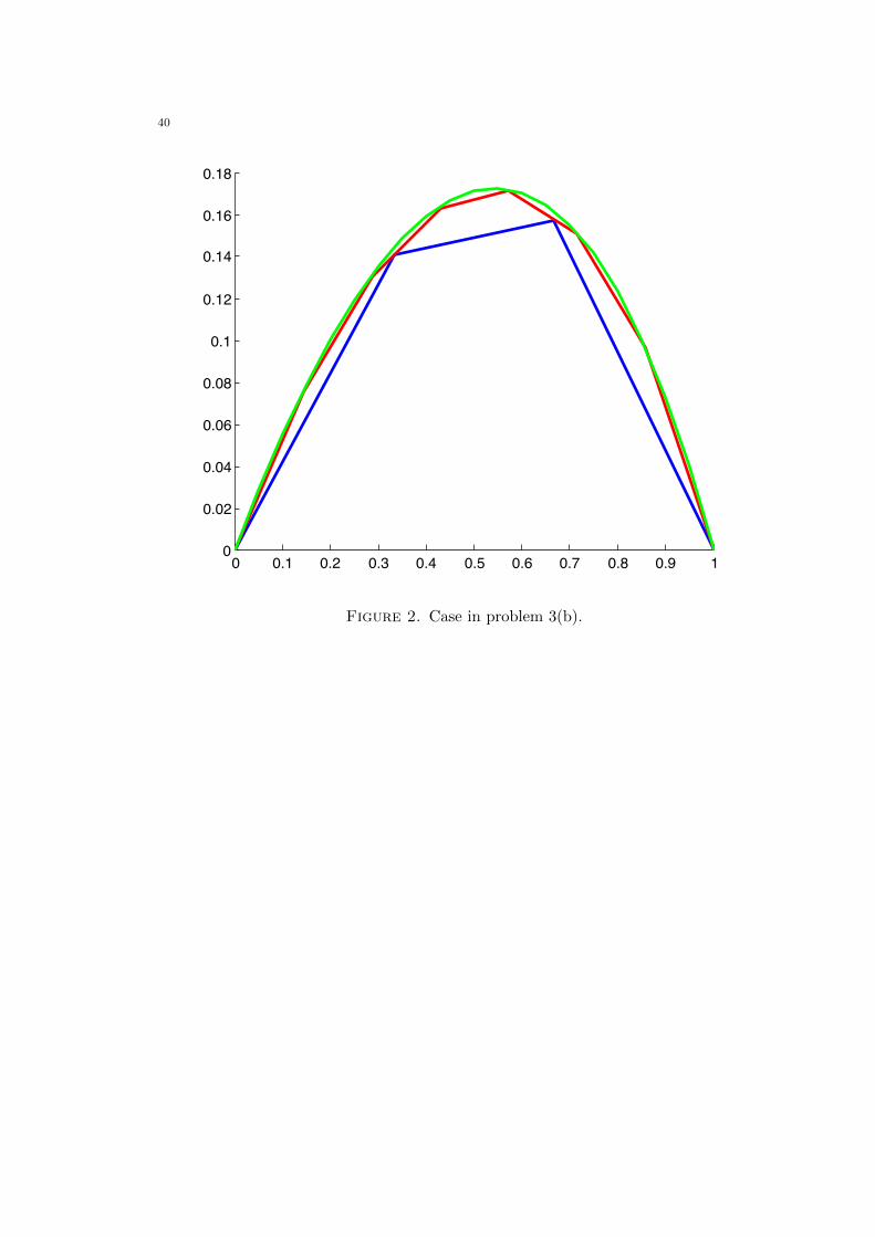
40

0 0.1 0.2 0.3 0.4 0.5 0.6 0.7 0.8 0.9 10

0.02

0.04

0.06

0.08

0.1

0.12

0.14

0.16

0.18

Figure 2. Case in problem 3(b).

41

0 0.1 0.2 0.3 0.4 0.5 0.6 0.7 0.8 0.9 10

0.05

0.1

0.15

0.2

0.25

Figure 3. Case in problem 3(c).

42

Essential Partial Differential Equations Examples 7

The exercises marked with ? are the most important.The first six exercises are related to the following eigenvalue problem: find all possiblepairs λ, u, where λ ∈ R and u : (0, 1)→ R is not identically equal to zero, such that

−u′′(x) = λ u(x) x ∈ (0, 1), (E)

together with the boundary conditions u(0) = 0 = u(1). The values of λ are calledeigenvalues and the corresponding functions u are called eigenfunctions.

(7.1) Show that the eigenfunctions are u(j)(x) = c sin(jπx) for j = 1, ... ,∞ andsome constant c 6= 0, and determine the corresponding eigenvalues. What is thesmallest eigenvalue λ(1)?

(7.2) Show that (λ, u) satisfying (E) also satisfies a weak formulation: find the pair(λ ∈ R, u 6= 0 ∈ H1

0 (0, 1)) such that∫ 1

0u′v′ dx = λ

∫ 1

0uv dx ∀v ∈ H1

0 (0, 1). (M)

(7.3) Show that any eigenvalue λ ∈ R satisfying (M) must satisfy λ > 0.(7.4) ? Given some finite dimensional subspace Hk ⊂ H1

0 (0, 1) with a basis set hjkj=1,

show that a Galerkin approximation to (M) can be found by solving the followinglinear algebra problem,

K x = λkQx (Mk)

where K is the k × k “stiffness” matrix with entries Kij =∫ 1

0 h′jh′i dx and Q is

the k × k “mass” matrix with entries Qij =∫ 1

0 hjhi dx.(7.5) Show that the matrices Q and K are both symmetric positive definite, and use

this to show that the eigenvalues λk satisfying (Mk) are all strictly positive.

(7.6) ? Hence, compute the Galerkin approximation of the smallest eigenvalue λ(1)

satisfying (E) in the case when Hk contains functions of the form

u3(x) = β1h1(x) + β2h2(x) + β3h3(x), β1, β2, β3 ∈ R,

where hi(x) are the continuous piecewise linear functions satisfying hi(xi) = 1with support [xi−1, xi+1] for four equal subintervals with nodes x0, . . . , x4. (Theeasiest way to solve the 3 × 3 problem (M3) is to use the MATLAB functioneig.)

(7.7) Write down the analytic solution of the ODE system: find u(t) ∈ R2 such that

du

dt=

(1 22 1

)u; t > 0; with u(0) =

(12

).

Can you determine an explicit solution? (Hint: Use the matrix exponential.)Note that calculation of the matrix exponential is nonexaminable.

(7.8) Suppose that B1 and B2 are k×k matrices. Show by equating terms in the seriesexpansions that if B1B2 = B2B1 then

eB1eB2 = eB1+B2 = eB2eB1 .

43

(7.9) ? Consider the generic initial value problem: given a matrix A ∈ Rk×k, initialdata u(0) ∈ Rk and a forcing function f(t), we seek u(t) such that

du

dt+Au = f , t ∈ (0, T ].

(i) Show that for t ≥ 0

|u(t)| ≤ |u(0)|+∫ t

0|f(s)| ds+ ‖A‖

∫ t

0|u(s)| ds

where ‖A‖ is the operator norm of A with | · | representing the l2 norm inRk.

(ii) The integral form of Gronwall’s inequality (see lecture 13) says that if ϕ isa nonegative continuous function such that

ϕ(t) ≤ a+ b

∫ t

0ϕ(s) ds, for t ∈ [0, T ].

with a and b nonnegative constants, then

ϕ(t) ≤ aebt, for t ∈ [0, T ].

Use this form of Gronwall’s inequality to establish the stability estimate

|u(t)| ≤ e‖A‖t(|u(0)|+

∫ t

0|f(s)| ds

)for all t ≥ 0.

44

Essential Differential Equations Solutions 7

(7.1) First consider the case λ < 0. The general solution of (E) in that case is

u(x) = a1 cosh(√−λ x

)+ a2 sinh

(√−λ x

).

The boundary condition u(0) = 0 implies a1 = 0, and the boundary conditionu(1) = 0 then implies that a2 = 0. Therefore when λ < 0 the only solution of (E)satisfying the boundary conditions is u(x) = 0. Thus there are no eigenvaluesless than zero.

Next suppose λ = 0. Then the general solution of (E) is

u(x) = a1x+ a2.

The boundary condition u(0) = 0 implies a2 = 0, and the boundary conditionu(1) = 0 then implies that a1 = 0. Therefore 0 is not an eigenvalue.

Now suppose λ > 0. The general solution is then

u(x) = a1 cos(√

λ x)

+ a2 sin(√

λ x).

The boundary condition u(0) = 0 implies that a1 = 0. The condition u(1) = 0implies that

sin(√

λ)

= 0,

and therefore√λ = jπ for some integer j. Thus the eigenfunctions are u(j)(x) =

a2 sin(jπx) as claimed. For each j the corresponding eigenvalue is

λj = j2π2.

Thus the smallest eigenvalue is λ(1) = π2 = 9.8696 · · · .(7.2) Note that u(j) ∈ C∞([0, 1]) and thus u(j) ∈ H1

0 (0, 1) for j = 1, 2, 3, . . .. Next,multiplying (E) by a test function v ∈ V and integrating by parts, we see thatthe pair (λ, u) satisfies the variational formulation (M).

(7.3) Setting v = u 6= 0 in (M) we see that λ =∫ 1

0 (u′)2/∫ 1

0 u2 = ‖u′‖2/‖u‖2 ≥ 0. We

can show that λ 6= 0 by contradiction. To this end we let λ = 0 which impliesthat ‖u′‖ = 0. Using the Poincare–Friedrichs inequality (valid for u ∈ H1

0 (0, 1))we then get

‖u‖ ≤ ‖u′‖ = 0.

Hence u = 0 almost everwhere!(7.4) The Galerkin approximation of (M) is: find the pair (λk ∈ R, uk ∈ Hk) such

that ∫ 1

0u′kv

′ = λk

∫ 1

0ukv ∀v ∈ Hk.

Given the basis set, the eigenfunction uk(x) can be uniquely written as

uk =

k∑j=1

βjhj .

45

To identify the corresponding linear algebra problem, we let v = hi so that∫ 1

0

k∑j=1

βjh′jh′i = λk

∫ 1

0

k∑j=1

βjhjhi

and we then write the integral of the sum as the sum of the integrals on both sidesof the equation. This leads to the generalized eigenvalue problem Kx = λkQx

with matrices Kij =∫ 1

0 h′jh′i and Qij =

∫ 10 hjhi and with the eigenvector x given

by the unknown coefficients

x =

β1...βk

.

(7.5) Premultiplying (Mk) by xT we see that the eigenvalue is given by the expressionλk = xTKx/xTQx. We deduce that λk must be strictly positive since xTKx > 0and xTQx > 0. (Note that x 6= 0.)

(7.6) To construct a finite element approximation we introduce basis functions h1(x), . . . , hn−1(x),which are the piecewise linear functions on the subdivision 0 = x0 < x1 < · · · <xn = 1, with hj(xi) = 0 for all i 6= j and hj(xj) = 1.

The stiffness matrix K was constructed in class (see lecture 9). For a uniformsubdivision of size h = 1

n it is the symmetric tridiagonal matrix with diagonal

entries Ki,i = 2h and off-diagonal entries Ki,i−1 = − 1

h = Ki,i+1.The mass matrix Q can be computed similarly: this time by integrating qua-

dratic polynomials in a piecewise fashion. As in the case of K, when |i− j| ≥ 1Qij = 0, and aside from this we only need to consider two cases:

Case 1 (i = j). In this case we have

Qjj =

∫ xj

xj−1

hj(x)2 dx+

∫ xj+1

xj

hj(x)2 dx

=

∫ xj

xj−1

(x− xj−1

h

)2

dx+

∫ xj

xj−1

(xj+1 − x

h

)2

dx

=

((x− xj−1)3

3h2

∣∣∣∣xjxj−1

−(

(xj−1 − x)3

3h2

∣∣∣∣xj+1

xj

=h

3+h

3=

2h

3.

Case 2 (j = i+ 1) In this case we have

Qi(i+1) =

∫ xi+1

xi

hi(x)hi+1 dx

=

∫ xi+1

xi

(xi+1 − x

h

)(x− xih

)dx.

46

We could multiply the integrand out, but is easier to change variables s = x−xito get

Qi(i+1) =1

h2

∫ h

0s(h− s) ds

=1

h2

(s2

2h− s3

3

∣∣∣∣h0

= h

(1

2− 1

3

)=h

6

From these calculations, using also the fact that Q is symmetric, we find thatQ is a tridiagonal matrix with diagonal entries Qi,i = 2h

3 and with off-diagonal

entries Qi,i−1 = h6 = Qi,i+1.

In the case of interest, h = 1/4, so the 3× 3 system takes the form 8 −4 0−4 8 −40 −4 8

β1

β2

β3

= λ

1/6 1/24 01/24 1/6 1/24

0 1/24 1/6

β1

β2

β3.

The system can be solved using MATLAB as follows.

>> h=1/4;

>> A=[2/h,-1/h,0;-1/h,2/h,-1/h;0,-1/h,2/h]

>> Q=[2*h/3,h/6,0;h/6,2*h/3,h/6;0,h/6,2*h/3]

>> lambda=eig(A,Q)

lambda =

10.3866

48.0000

126.7562

Thus we deduce that the finite element estimate of the smallest eigenvalue λ(1)

is lambda(1)= 10.3866.To get a more accurate answer we must take a finer subdivision. Repeating the

calculation with h = 1/128 gives the estimate λ(1) ≈ 9.8701 which is accurate tothree decimal places.

(7.7) The solution of the ODE system dudt = Au is given by u(t) = eAtu(0). In this

example we have the symmetric matrix

A =

(1 22 1

).

The simplest way to solve the ODE system is to diagonalise A by computingthe eigenvalues and normalized eigenvectors. This results in the matrix decom-position A = XTDX with(

1 22 1

)=

(1/√

2 1/√

2

−1/√

2 1/√

2

)(−1 00 3

)(1/√

2 −1/√

2

1/√

2 1/√

2

)

47

Note that, since A is a symmetric matrix, the eigenvector matrix X is orthogonal,that is X−1 = XT (to check, simply compute XTX). Now we have

eAt =

(1/√

2 1/√

2

−1/√

2 1/√

2

)(e−t 00 e3t

)(1/√

2 −1/√

2

1/√

2 1/√

2

)=

1

2

(e−t + e3t −e−t + e3t

−e−t + e3t e−t + e3t

).

The solution of the initial value problem is thus

u(t) = eAtu(0)

=1

2

(e−t + e3t −e−t + e3t

−e−t + e3t e−t + e3t

)(12

)=

1

2

(−e−t + 3e3t

e−t + 3e3t

).

(7.8) We want to show that

eB1eB2 = eB1+B2 = eB2eB1 .

The key point here is that if B1 and B2 commute then

(B1 +B2)j =

j∑k=0

(j

k

)Bk

1Bj−k2 .

Otherwise, if B1 and B2 do not commute then for example

(B1 +B2)2 = B21 +B1B2 +B2B1 +B2

2 6= B21 + 2B1B2 +B2

2 !

We will establish equality using the series definition of the matrix exponential,thus

eB1+B2 =

∞∑j=0

1

j!(B1 +B2)j

=

∞∑j=0

1

j!

j∑k=0

(j

k

)Bk

1Bj−k2 =

∞∑j=0

j∑k=0

1

k!(j − k)!Bk

1Bj−k2

=

∞∑k=0

∞∑m=0

1

k!m!Bk

1Bm2 =

∞∑k=0

1

k!Bk

1

∞∑m=0

1

m!Bm

2

= eB1eB2

♥(7.9) (i) If we integrate the system of ODEs from 0 to t we obtain, using the funda-

mental theorem of calculus,

u(t)− u(0) = A

∫ t

0u(s) ds+

∫ t

0f(s) ds.

48

Now moving the u(0) to the other side, taking the norm, and using thetriangle inequality we have

|u(t)| ≤ |u(0)|+∣∣∣∣∫ t

0f(s) ds

∣∣∣∣+

∣∣∣∣A∫ t

0u(s) ds

∣∣∣∣ .Finally we can apply the property of the operator norm |Ax| ≤ ‖A‖|x|, andthe fact ∣∣∣∣∫ t

0u(s) ds

∣∣∣∣ ≤ ∫ t

0|u(s)| ds

to complete the proof.(ii) From part (a) we have

|u(t)| ≤ |u(0)|+∫ t

0|f(s)| ds+‖A‖

∫ t

0|u(s)| ds ≤ |u(0)|+

∫ T

0|f(s)| ds+‖A‖

∫ t

0|u(s)| ds

for any T ≥ t. Applying the integral form of Gronwall’s inequality withϕ(t) = |u(t)| and b = ‖A‖ > 0 we have

ϕ(t) ≤ e‖A‖t(|u(0)|+

∫ T

0|f(s)| ds

)for all t ∈ [0, T ]. Setting t = T gives the desired estimate.

49

Essential Partial Differential Equations Examples 8

The exercises marked with ? are the most important.

(8.1) Read the online notes on separation of variables for the heat equation.(8.2) ? Consider the heat equation in R1. Let I = [0, T ] represent a time interval,

let u0(x), x ∈ [0, 1] be the initial condition and define a Galerkin approxima-tion space Hh ⊂ H1

0 (0, 1). The semi-discretized problem is: for t ∈ I, we seekuh(x, t) ∈ Hh satisfying(

∂uh∂t

, vh

)+

(∂uh∂x

,∂vh∂x

)= 0 ∀vh ∈ Hh,

(uh(x, 0), vh) = (u0, vh) ∀vh ∈ Hh,

where (·, ·) is the standard L2(0, 1) inner product and ‖·‖ is the associated norm.Recall, see lecture ??, that this is equivalent to the semi-discrete system of ODEs

(IV P )

Qx′(t) = −Kx(t)Qx(0) = f .

(i) Let I be divided equally into time steps with length dt so that 0 = t0 <t1 < t2 < . . . < tn = T and tj − tj−1 = dt for all j. Find a fully discreteapproximation implicit approximation scheme by integrating the ODE in(IV P ) from tj−1 to tj , and applying the trapezoid rule to approximate theintegral. Write down the resulting time stepping rule (also referred to asthe Crank–Nicolson method).

(ii) Let ujh ∈ Hh be the implicit approximations given by the method found inpart (a) at tj . Establish that the scheme from part (a) is unconditionallystable: ∥∥∥ujh∥∥∥ ≤ ∥∥∥uj−1

h

∥∥∥ ≤ . . . ≤ ∥∥u0h

∥∥ .The remaining exercises are dedicated to implementation of the numerical methods wehave covered for approximating solutions of the heat equation in MATLAB. We alsodiscuss this in lecture ??.

(8.3) We will implement all three methods, Euler (see lecture ??), Backwards Eu-ler (see lecture ??), and Crank-Nicolson (see exercise 8.2), for time discretisa-tion. Therefore create three mfiles named respectively Eheat.m, BEheat.m, andCNheat.m. Begin the files by inputting the basic parameters for each methodwhich are

%Set spatial and temporal discretisation.

n = 6; %Number of subintervals in spatial discretisation is N = 2*n

dt = 0.001; %Set time step

nsteps = 50; %Number of time steps

N = 2*n; %Number of subintervals

h = 1/N; %Length of subintervals

Note we take the number of subintervals N to be 2 ∗ n so that N is an evennumber. It is easiest to work only in one of the three mfiles, and then copy thecode into the others since it is almost all the same for all three cases.

50

(8.4) Use the same method you used on exercise 6.2 to enter the matrices

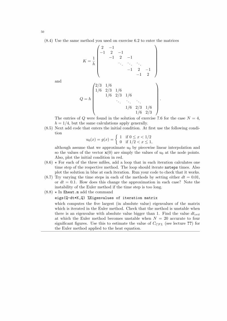
K =1

h

2 −1−1 2 −1

−1 2 −1. . .

. . .. . .

−1 2 −1−1 2

and

Q = h

2/3 1/61/6 2/3 1/6

1/6 2/3 1/6. . .

. . .. . .

1/6 2/3 1/61/6 2/3

.

The entries of Q were found in the solution of exercise 7.6 for the case N = 4,h = 1/4, but the same calculations apply generally.

(8.5) Next add code that enters the initial condition. At first use the following condi-tion

u0(x) = g(x) =

1 if 0 ≤ x < 1/20 if 1/2 < x ≤ 1,

although assume that we approximate u0 by piecewise linear interpolation andso the values of the vector x(0) are simply the values of u0 at the node points.Also, plot the initial condition in red.

(8.6) ? For each of the three mfiles, add a loop that in each iteration calculates onetime step of the respective method. The loop should iterate nsteps times. Alsoplot the solution in blue at each iteration. Run your code to check that it works.

(8.7) Try varying the time steps in each of the methods by setting either dt = 0.01,or dt = 0.1. How does this change the approximation in each case? Note theinstability of the Euler method if the time step is too long.

(8.8) ? In Eheat.m add the command

eigs(Q-dt*K,Q) %Eigenvalues of iteration matrix

which computes the five largest (in absolute value) eigenvalues of the matrixwhich is iterated in the Euler method. Check that the method is unstable whenthere is an eigenvalue with absolute value bigger than 1. Find the value dtcritat which the Euler method becomes unstable when N = 20 accurate to foursignificant figures. Use this to estimate the value of CCFL (see lecture ??) forthe Euler method applied to the heat equation.

51

Essential Differential Equations Solutions 8

(8.1) When you have finished reading the notes you can treat yourself to a mince pie.♥

(8.2) (i) As suggested in the problem, we integrate the system of ODEs over onetime step to obtain∫ tj

tj−1

Qx′(t) dt = −∫ tj

tj−1

Kx(t) dt⇔ Qx(tj)−Qx(tj−1) = −∫ tj

tj−1

Kx(t) dt.

For the fully discrete scheme we approximate the integral in this last equa-tion using the trapezoid rule∫ tj

tj−1

Kx(t) dt ≈ dt

2(Kx(tj) +Kx(tj−1))

Thus if xj−1 ≈ x(tj−1) then we find xj ≈ x(tj) using the formula

Qxj −Qxj−1 = −dt2

(Kxj +Kxj−1)⇔(Q+

dt

2K

)xj =

(Q− dt

2K

)xj−1.

For each time step we use this rule.(ii) To establish the stability of the method we follow a similar procedure to

that used in the proof of stability for the backwards Euler method fromlecture ??. We start by multiplying the time step rule by (xj + xj−1)T toobtain

(xj + xj−1)TQxj +dt

2(xj + xj−1)TKxj = (xj + xj−1)TQxj−1 −

dt

2(xj + xj−1)TKxj−1.

Rearranging we find that

xTj Qxj +dt

2(xj + xj−1)TK(xj + xj−1) = xTj−1Qxj−1.

Since K is positive definite we have

xTj Qxj ≤ xTj−1Qxj−1.

The last inequality is equivalent to

‖ujk‖2L2(0,1) ≤ ‖u

j−1k ‖2L2(0,1).

This completes the proof.(8.3) On this part, simply follow the instructions given in the question.(8.4) The following code constructs the matrices:

%Construct stiffness matrix K

K = diag(2*ones(N-1,1));%Put 2’s on main diagonal

K = K+diag(-ones(N-2,1),-1); %Put -1’s below main diagonal

K = K+diag(-ones(N-2,1),1); %Put -1’s above main diagonal

K = 1/h*K;

%Construct mass matrix Q

Q = diag(2/3*ones(N-1,1));%Put 2/3’s on main diagonal

Q = Q+diag(1/6*ones(N-2,1),-1); %Put 1/6’s below main diagonal

Q = Q+diag(1/6*ones(N-2,1),1); %Put 1/6’s above main diagonal

52

Q = h*Q;

(8.5) The following code can be used for this part:

u0 = [ones(N/2,1);zeros(N/2+1,1)]; %Initial condition

x = u0(2:N); %x0, assume u0 already piecewise linear.

clf; %Clear figure

nodes=(0:h:1)’; %Vector containing spatial node positions

plot(nodes,u0,’-r’), axis square %Plot u0

set(gca, ’Ylim’,[-.2,1.2]), shg

xlabel(’x’), ylabel(’uh’), hold all %Plot options

Note that the option ’-r’ in the plot command makes the red plot. We use holdall so that the later plots will appear on the same axes with the same options.Also, note that u0 includes the values at the two endpoints, while the vector x

does not.(8.6) The following code works for the case of the Euler method

for k=1:nsteps, % time step loop

x=Q\((Q-dt*K)*x); % Euler method time step

cla %clear axes

plot(nodes,u0,’-r’) %plot initial condition again in red

plot(nodes,[0;x;0],’-b’), axis square, shg, pause(.1) %plot approximation

end

For the backwards Euler and Crank-Nicolson methods simply replace the singleline marked Euler method time step with one of the following:

x=(Q+dt*K)\(Q*x); % backwards Euler method time step

or

x=(Q+0.5*dt*K)\((Q-0.5*dt*K)*x); % Crank-Nicolson time step

(8.7) Follow the instructions in the question and observe the results.(8.8) Note that for N = 20, we set n = 10 in the parameters at the beginning of the

mfile. It is not too hard to find dtcrit at which the Euler method loses stabilityby simply checking the eigenvalues for many different possible dt. Doing thisyou can find that the Euler method is stable for dt= 0.0004244 and unstable fordt= 0.0004245. For this value of N , h = 1/N = 0.05, and so we estimate CCFLfrom this to be

CCFL ≈dtcrith2≈ 0.0004244

(0.05)2≈ 0.1698.