Essays on Time-Varying Discount Rates

CitationDew-Becker, Ian. 2012. Essays on Time-Varying Discount Rates. Doctoral dissertation, Harvard University.

Permanent linkhttp://nrs.harvard.edu/urn-3:HUL.InstRepos:9306478

Terms of UseThis article was downloaded from Harvard University’s DASH repository, and is made available under the terms and conditions applicable to Other Posted Material, as set forth at http://nrs.harvard.edu/urn-3:HUL.InstRepos:dash.current.terms-of-use#LAA

Share Your StoryThe Harvard community has made this article openly available.Please share how this access benefits you. Submit a story .

Accessibility

©2012 — Ian Louis Dew-Becker

All rights reserved.

Dissertation Advisor: Professor John Y. Campbell Ian Louis Dew-Becker

Essays on Time-Varying Discount Rates

ABSTRACT

This dissertation consists of three essays that explore the interaction between various

discount rates and the macroeconomy.

The first essay studies the cross-section of discount rates, specifically, the term structure

of interest rates. When physical capital is discounted like a bond with a similar duration,

a high term spread is associated with low average duration for investment. I document a

strong negative correlation between the term spread and the duration of investment, im-

plying an important role for the cost of capital in determining the composition of aggregate

investment. The results are robust to including a variety of controls. Consumer durable

goods purchases display similar behavior.

The second essay develops a new utility specification that incorporates Campbell–

Cochrane–type habits into the Epstein–Zin class of preferences. It is a model in which

risk premia change over time. In a simple calibration of a real business cycle model with

EZ-habit preferences, the model generates a strongly countercyclical equity premium, sub-

stantial equity return predictability, and a stable riskless interest rate, as in the data. More-

over, conditional on the average level of risk aversion, time-variation in risk aversion in-

creases the volatility and mean return of equities. On the real side, the model matches

the short and long-term variances of output, consumption, and investment growth. As an

additional empirical test, I measure implied risk aversion and find that it has an R² of over

50 percent for 5-year stock returns in post-war data.

The third essay develops a New-Keynesian model in which households have Epstein–

Zin preferences with time-varying risk aversion and the central bank has a time-varying

inflation target. The model matches the dynamics of nominal bond prices in the US econ-

omy well: the fitting errors for individual bond yields are roughly as large as those ob-

iii

tained from a non-structural three-factor model, and two thirds smaller than in models

with constant risk aversion or a constant inflation target.

iv

CONTENTS

Abstract . . . . . . . . . . . . . . . . . . . . . . . . . . . . . . . . . . . . . . . . . . . . . iii

Acknowledgments . . . . . . . . . . . . . . . . . . . . . . . . . . . . . . . . . . . . . . . . vii

1. Investment and the Cost of Capital in the Cross-Section: The Term Spread Predicts the

Duration of Investment . . . . . . . . . . . . . . . . . . . . . . . . . . . . . . . . . . . 1

1.1 Introduction . . . . . . . . . . . . . . . . . . . . . . . . . . . . . . . . . . . . . 1

1.2 Data . . . . . . . . . . . . . . . . . . . . . . . . . . . . . . . . . . . . . . . . . . 5

1.3 Results . . . . . . . . . . . . . . . . . . . . . . . . . . . . . . . . . . . . . . . . 12

1.4 Model . . . . . . . . . . . . . . . . . . . . . . . . . . . . . . . . . . . . . . . . . 14

1.5 Alternative explanations . . . . . . . . . . . . . . . . . . . . . . . . . . . . . . 19

1.6 Consumer durables . . . . . . . . . . . . . . . . . . . . . . . . . . . . . . . . . 27

1.7 The firm-level mechanism . . . . . . . . . . . . . . . . . . . . . . . . . . . . . 29

1.8 Conclusion . . . . . . . . . . . . . . . . . . . . . . . . . . . . . . . . . . . . . . 37

2. A model of time-varying risk premia with habits and production . . . . . . . . . . . . . 39

2.1 Introduction . . . . . . . . . . . . . . . . . . . . . . . . . . . . . . . . . . . . . 39

2.2 The model . . . . . . . . . . . . . . . . . . . . . . . . . . . . . . . . . . . . . . 44

2.3 Calibration and simulation . . . . . . . . . . . . . . . . . . . . . . . . . . . . . 51

2.4 Empirical return forecasting . . . . . . . . . . . . . . . . . . . . . . . . . . . . 72

2.5 Extensions . . . . . . . . . . . . . . . . . . . . . . . . . . . . . . . . . . . . . . 81

2.6 Conclusion . . . . . . . . . . . . . . . . . . . . . . . . . . . . . . . . . . . . . . 91

3. Bond pricing with a time-varying price of risk in an estimated medium-scale Bayesian

DSGE model . . . . . . . . . . . . . . . . . . . . . . . . . . . . . . . . . . . . . . . . 93

v

3.1 Introduction . . . . . . . . . . . . . . . . . . . . . . . . . . . . . . . . . . . . . 93

3.2 Household preferences . . . . . . . . . . . . . . . . . . . . . . . . . . . . . . . 97

3.3 Aggregate supply . . . . . . . . . . . . . . . . . . . . . . . . . . . . . . . . . . 101

3.4 Model solution . . . . . . . . . . . . . . . . . . . . . . . . . . . . . . . . . . . 108

3.5 Empirics . . . . . . . . . . . . . . . . . . . . . . . . . . . . . . . . . . . . . . . 112

3.6 Asset pricing . . . . . . . . . . . . . . . . . . . . . . . . . . . . . . . . . . . . . 118

3.7 The real economy . . . . . . . . . . . . . . . . . . . . . . . . . . . . . . . . . . 137

3.8 Conclusion . . . . . . . . . . . . . . . . . . . . . . . . . . . . . . . . . . . . . . 143

Appendix 146

A. Appendix to Chapter 1 . . . . . . . . . . . . . . . . . . . . . . . . . . . . . . . . . . . 147

A.1 The approximation for average duration . . . . . . . . . . . . . . . . . . . . . 147

A.2 Further robustness tests . . . . . . . . . . . . . . . . . . . . . . . . . . . . . . 148

B. Appendix to chapter 2 . . . . . . . . . . . . . . . . . . . . . . . . . . . . . . . . . . . . 150

B.1 The certainty equivalent . . . . . . . . . . . . . . . . . . . . . . . . . . . . . . 150

B.2 Derivation of the SDF . . . . . . . . . . . . . . . . . . . . . . . . . . . . . . . . 152

B.3 The log-linear model with production . . . . . . . . . . . . . . . . . . . . . . 153

B.4 Details of return forecasting . . . . . . . . . . . . . . . . . . . . . . . . . . . . 165

C. Appendix to Chapter 3 . . . . . . . . . . . . . . . . . . . . . . . . . . . . . . . . . . . 175

C.1 Results from the text . . . . . . . . . . . . . . . . . . . . . . . . . . . . . . . . 175

C.2 Approximation method . . . . . . . . . . . . . . . . . . . . . . . . . . . . . . 177

C.3 Estimation . . . . . . . . . . . . . . . . . . . . . . . . . . . . . . . . . . . . . . 182

vi

ACKNOWLEDGMENTS

I completed this dissertation with the support of many people. John Campbell was

endlessly patient, and amazingly diligent about reading and commenting on any work I

sent him. He went above and beyond any reasonable expectation. I also benefited from

numerous comments and conversations with my other advisors, Emmanuel Farhi, Effi

Benmelech, and also David Laibson, Robin Greenwood, and Jim Stock, among others.

Countless conversations with fellow students made this possible, including in particular

Jason Beeler, Stefano Giglio, Kelly Shue, and Eric Zwick. Economists too numerous to

name also generously gave me constant feedback on my work which is reflected here. But

none of the above should be implicated in any errors or omissions.

vii

1. INVESTMENT AND THE COST OF CAPITAL IN THE CROSS-SECTION: THE TERM

SPREAD PREDICTS THE DURATION OF INVESTMENT

1.1 Introduction

This paper studies the cross-section of investment. While there is an enormous amount

of work studying the aggregate level of investment and the determinants of firm-level

investment, there is essentially no analysis of the determinants of investment in different

types of assets. This paper begins that task by analyzing the distribution of investment

across assets according to their depreciation rates. I show that when interest rates for long-

duration assets are higher than those for short-duration assets, aggregate investment shifts

relatively towards high-depreciation assets.

The response of investment to the cost of capital is a key mechanism in macroeconomics

and finance. It is central to production-based asset pricing theories (e.g. Cochrane 1991,

1996); a primary feedback mechanism in standard general-equilibrium models; one of the

key drivers for the response of the economy to monetary policy shocks; the source of the

classical crowding-out effect of government spending; and an important determinant of

the size of distortions from taxes. This paper considers a novel method for uncovering an

empirical relationship between investment and the cost of capital.

There is a long literature that studies the effect of the cost of capital on investment. Sim-

ple methods have, in general, failed to find important effects.1 Bernanke and Gertler (1995)

find that nonresidential investment seems to respond only weakly to shocks to the Federal

funds rate.2 The discount rate is also a determinant of Tobin’s Q, but estimates of the im-

pact of Q on investment tend to be small (Summers, 1981; Eberly, Rebelo, and Vincent,

1 See Chirinko, 1993, for an extensive review.

2 However, in recent unpublished papers, Gilchrist and Zakrajsek (2008) and Guiso et al. (2002) find arelationship in micro data between investment and interest rates.

1

2009, give a recent review). The primary contribution of this paper is to show that interest

rates affect what assets firms invest in at the aggregate level. Furthermore, the effect is rel-

evant at the cyclical frequency: it is neither centered around discrete (and somewhat rare)

policy changes, such as tax changes, or dependent on very long-term effects.3

The basic idea here is to forecast the cross-section of investment using the cross-section

of interest rates, instead of forecasting the level of investment with the level of interest

rates. Long-term assets are discounted with long-term interest rates, and short-term assets

with short rates. When long rates are higher than short rates—the term spread is high—a

cost-of-capital effect implies investment should shift towards short-duration assets. The

negative relationship holds strongly in the data: it explains roughly one third of the cross-

sectional variation in investment by duration, and the effect holds both within and across

industries.

Standard regressions of aggregate investment on the level of interest rates have the

fundamental identification problem that periods of high interest rates may also be periods

when investment demand is high, so the correlation between investment and interest rates

could be zero or even positive. By studying the cross-section, I abstract from aggregate

shocks, hopefully reducing this endogeneity problem. The strong empirical results suggest

that in fact endogeneity is less of an issue in the cross-section.

The data is simple to construct. I obtain nominal investment by asset and year from the

Bureau of Economic Analysis. I study an index of average duration defined as the average

the of the assets’ economic life-spans, weighted by their share in aggregate investment

in each year.4 Figure 1.1 shows that this index of average duration is highly negatively

correlated with the spread between interest rates on ten and one-year nominal Treasury

bonds (note that the axis for average duration is reversed for the sake of clarity). When

interest rates are relatively high for long-duration assets, investment shifts towards short-

duration assets, creating a strong negative correlation between average duration and the

3 Caballero (1994) and Schaller (2006) use cointegration methods to show that in the long run the cost ofcapital is meaningfully related to the size of the capital stock (and hence the level of investment). A numberof researchers have also focused on high-frequency changes in taxes which produce large movements in thecost of capital and investment (Hassett and Hubbard, 2002, provide an extensive review).

4 Specifically, "lifespan" is measured as a Macaulay duration using data on economic depreciation rates.

2

term spread.

A negative raw correlation between investment and interest rates suggests that the cost

of capital has an important role in determining the cross-sectional distribution of invest-

ment, but there are alternative mechanisms that could produce this result. I therefore build

a simple Q-theory model to help elucidate the possible sources of bias in the basic result in

figure 1.1 and try to account for them in subsequent regressions. I control for the level of

productivity and expected productivity growth in a variety of ways and find that they do

not eliminate the basic effect. More importantly, I find that the term spread–average du-

ration relationship is not driven by changes in demand across industries. When the term

spread is high, investment shifts towards low-duration assets within individual industries,

in addition to shifting from industries that use more long-duration assets to ones that use

more short-duration assets.

In addition to contributing to the literature on the determinants of the level of invest-

ment, this paper is related to the recent literature on production-based asset pricing with

projects that have differing characteristics (e.g. Berk, Green, and Naik, 1999, and Gomes,

Kogan, and Yogo, 2009). While those papers show that variation in the types of capital

owned by firms can lead to differences in their stock prices, I find that variation in the

cross-section of asset prices can affect the types of investment that firms undertake.

The findings here are also relevant to understanding the relationship between interest

rates and debt issues. The final section of the paper provides novel evidence that firms

match the maturity of their debt issues to their physical investment, consistent previous

evidence in the finance literature (e.g. Stohs and Mauer, 1996). My findings suggest that

the timing of debt issues to the term spread documented by Baker, Greenwood, and Wur-

gler (2003) could be explained by the dynamics of physical investment and the fact that

firms match the maturity of their debt to their assets.

The remainder of the paper is organized as follows. Section 1.2 describes the data and

section 1.3 reports the main result. Next, I outline in section 1.4 a simple model that jus-

tifies the regression of the average duration of investment on the term spread. Section 1.5

controls for a number of possible biases suggested by the investment model and shows

that the term spread is the single most powerful predictor of the average duration of in-

3

Figu

re1.

1:Th

eav

erag

edu

rati

onof

inve

stm

entv

ersu

sth

ete

rmsp

read

-0.2

-0.15

-0.1

-0.05

0 0.05

-0.50

0.51

1.52

1948

1953

1958

1963

1968

1973

1978

1983

1988

1993

1998

2003

Duration

Term Spread

Term Spread

0.1 0.15

0.2

-2

-1.5-1

Average Duration

Note: The term

spread

is the ga

p between the 10 and 1-year treasu

ry yields av

erag

ed over the previous year. Both variables are HP-detrended

. The

axis for av

erag

e duration is reversed. Grey bars indicate NBER-dated

recessions.

4

vestment. In section 1.6 I show that the relationship between duration and the term spread

also appears in purchases of consumer durable goods. Section 1.7 examines the relation-

ship between the type of debt that firms sell and the duration of their assets. I find a posi-

tive relationship (consistent with maturity-matching theories), which gives added support

for the idea that long-term interest rates are the relevant cost of capital for long-duration

assets and short rates for short-term assets. Finally, section 1.8 concludes.

1.2 Data

To study the relationship between investment and the cost of capital in the cross-

section, we need a relevant measure of the cost of capital that differs across assets. The du-

ration of assets is a natural source of variation because it is easy to quantify for both phys-

ical assets (through their depreciation rates) and bonds (through maturities). Of course,

the cost of capital depends on more than simply the level of interest rates. The equity pre-

mium is large and variable (e.g. Lettau and Ludvigson, 2001). The advantage of focusing

on interest rates here is that we can directly observe the cost of capital for assets of differ-

ent durations. While there have been studies of the term structure of equity (Lettau and

Wachter, 2007), there is no simple way to actually measure the term structure of expected

returns on equity, let alone the variation in the slope of that term structure.

I obtain data on Treasury yields measured at year-end from the Federal Reserve. Trea-

sury data has the advantage of including bonds with a large variety of maturities over a

long period of time. However, firms do not in general borrow at the Treasury yield. I there-

fore also study the spread between yields on 3-month commercial paper and the Moody’s

seasoned Baa corporate bond yield (from Global Financial Data and the Federal Reserve,

respectively). The Moody’s index is meant to measure bonds with remaining maturities

near 30 years. The main results focus on the Treasury yield spread.5

A potential concern is that the relevant discount rate for investment is the real inter-

est rate, not the nominal rate. One method for obtaining the real interest rate would be

5 Ideally, we would measure the true cost of capital for each asset, including the cost of capital for equity, inparticular. While there is research on the term structure for equity (Lettau and Wachter, 2007), it is not obvioushow to construct an equity cost of capital for each asset simply by looking at its depreciation rate.

5

to subtract an inflation forecast from the nominal rate. In general, random-walk inflation

forecasts are competitive with more sophisticated methods (Atkeson and Ohanian, 2001).

With a random-walk forecast, the nominal term spread and the spread obtained after sub-

tracting expected inflation will be identical, which suggests that there is little to be gained

by forecasting inflation here.6

Another option is to look at yields on inflation-protected bonds. The time series of

inflation-protected bonds in the United States is relatively short, but inflation protected

bonds have been sold in the United Kingdom since the 1980’s. Figure 1.2 plots the 10/5

year term spread in the UK for both nominal and inflation-protected bonds since 1985.

Over the sample, the two series move together closely, even through the financial crisis.

Their variances differ, but they are over 70 percent correlated. This result suggests that

by studying the nominal term spread, we will obtain results that are similar to what we

would obtain with the unobservable real term spread.

Data on capital stocks and investment come from the Bureau of Economic Analysis’s

(BEA) fixed asset tables. The main results focus on aggregate investment by asset, but

the BEA also reports data at the asset×industry level. Data on depreciation rates is from

Fraumeni (1997), the source for current depreciation rates used by the BEA.7 The BEA uses

geometric (declining balance) depreciation for nearly all assets.8 Depreciation rates are

estimated primarily from data on service lives and sales of vintage assets. Given the resale

value of an asset for each age along with a service life, one can estimate an approximate

geometric depreciation rate.9 These depreciation rates are closer to economic depreciation

than the straight-line method used for accounting purposes by many firms (Hulten and

Wykoff, 1981).

I use 36 asset classes from the BEA tables, excluding household and government as-

6 Furthermore, we would need to estimate a 10-year inflation forecast, which would be difficult even ifinflation were relatively easy to forecast at short horizons. Another option would be to use survey data oninflation forecasts, but this would substantially limit the available time series.

7 Her depreciation rates closely match depreciation obtained by simply diving BEA reported depreciationby the capital stock.

8 Missiles and nuclear fuel rods, for example, are modeled with straight-line depreciation.

9 The BEA’s current estimates are a combination of data from a variety of studies on resale values reviewedin Fraumeni, 1997.

6

Figu

re1.

2:U

nite

dK

ingd

om10

/5ye

arte

rmsp

read

s,19

85–2

010

-0.50

0.51

1.52 1/

851/

901/

951/

001/

051/

10

Nom

inal

-2

-1.5-1

Inflat

ion-a

dju

sted

Note

: gap

bet

wee

n y

ield

s on 1

0 an

d 5

-yea

r nom

inal a

nd inflat

ion-p

rote

cted

bonds

7

sets and educational, health, and religion-related structures. The majority of the analysis

focuses on equipment investment. The investment literature generally finds that models

have substantial trouble explaining structures investment (Oliner, Rudebusch, and Sichel,

1995). This may be partly caused by the fact that nonresidential building projects take four-

teen months to complete on average (Edge, 2000).10 The main results below go through

when structures are included, but the relationships are far less clear. I therefore leave

the analysis of structures to future work so as not to distract from a complete analysis of

equipment investment.

For each asset class, the BEA reports total stocks (on a current-cost basis) and invest-

ment for the private nonresidential economy. The asset classes accounting for the most

nominal investment in 2007 were software (16 percent of total investment), petroleum

and natural gas exploration and wells (8 percent), communication equipment (7 percent),

and computers and peripheral equipment (6 percent). Except for oil and gas, these assets

all have high depreciation rates, and substantial investment is necessary just to keep the

stocks at constant levels.

For an asset with geometric depreciation rate δi, if we assume that productivity is con-

stant and there is a fixed discount rate r∗, Macaulay’s duration, Di, will be

Di =∞

∑j=1

j(1− δi)

j−1

(1 + r∗)j =1 + r∗

r∗ + δi(1.1)

When measuring durations I fix r∗ = 0.03.11 Table 1.1 lists the assets used in this study

along with their depreciation rates and durations. Software, computers, and office and

accounting equipment have the highest depreciation rates, all above 20 percent per year.

Types of heavy industrial machinery tend to have lower depreciation rates, as low as 5

percent.

Finally, for the purpose of summarizing the cross-section of investment, I define an

10 See Edge (2000) for an empirical model of residential and nonresidential structures investment that takesinto account building lags.

11 Allowing for a constant rate of productivity growth would be the equivalent of choosing a lower value ofr∗. The results are not sensitive to the choice of r∗.

8

Table 1.1: Assets, depreciation rates, and durations

Depreciation

rate (percent)

Duration

(years)

Asset

Information processing equipment and software

0.25 3.73 Computers and peripheral equipment

0.40 2.37 Software

0.14 6.11 Communication equipment

0.14 6.24 Medical equipment and instruments

0.14 6.24 Nonmedical instruments

0.18 4.90 Photocopy and related equipment

0.31 3.01 Office and accounting equipment

Industrial equipment

0.09 8.46 Fabricated metal products

0.05 12.62 Engines and turbines

0.12 6.75 Metalworking machinery

0.10 7.74 Special industry machinery, n.e.c.

0.11 7.51 General industrial, including materials handling, equipment

0.05 12.88 Electrical transmission, distribution, and industrial apparatus

Transportation equipment

0.15 5.72 Trucks, buses, and truck trailers

0.22 4.12 Autos

0.12 7.10 Aircraft

0.06 11.31 Ships and boats

0.06 11.59 Railroad equipment

Other equipment

0.14 6.15 Furniture and fixtures

0.12 6.87 Agricultural machinery

0.16 5.51 Construction machinery

0.15 5.72 Mining and oilfield machinery

0.16 5.42 Service industry machinery

0.18 4.83 Electrical equipment, n.e.c.

0.15 5.81 Other nonresidential equipment

Structures

0.02 18.83 Office, including medical buildings

0.02 19.73 Commercial

0.03 16.89 Manufacturing

0.02 19.18 Electric

0.02 19.18 Other power

0.02 19.18 Communication

0.08 9.80 Petroleum and natural gas

0.05 13.73 Mining

0.02 19.62 Other buildings

0.03 17.91 Railroads

0.02 19.11 FarmNote: Depreciation rates are otained from the BEA. Duration is measured as 1.03/(0.03+δ).

9

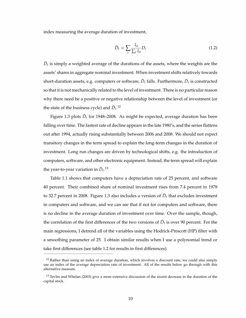
index measuring the average duration of investment,

Dt ≡∑i

Iit

∑i IitDi (1.2)

Dt is simply a weighted average of the durations of the assets, where the weights are the

assets’ shares in aggregate nominal investment. When investment shifts relatively towards

short-duration assets, e.g. computers or software, Dt falls. Furthermore, Dt is constructed

so that it is not mechanically related to the level of investment. There is no particular reason

why there need be a positive or negative relationship between the level of investment (or

the state of the business cycle) and Dt.12

Figure 1.3 plots Dt for 1948–2008. As might be expected, average duration has been

falling over time. The fastest rate of decline appears in the late 1980’s, and the series flattens

out after 1994, actually rising substantially between 2006 and 2008. We should not expect

transitory changes in the term spread to explain the long-term changes in the duration of

investment. Long run changes are driven by technological shifts, e.g. the introduction of

computers, software, and other electronic equipment. Instead, the term spread will explain

the year-to-year variation in Dt.13

Table 1.1 shows that computers have a depreciation rate of 25 percent, and software

40 percent. Their combined share of nominal investment rises from 7.4 percent in 1978

to 32.7 percent in 2008. Figure 1.3 also includes a version of Dt that excludes investment

in computers and software, and we can see that if not for computers and software, there

is no decline in the average duration of investment over time. Over the sample, though,

the correlation of the first differences of the two versions of Dt is over 90 percent. For the

main regressions, I detrend all of the variables using the Hodrick-Prescott (HP) filter with

a smoothing parameter of 25. I obtain similar results when I use a polynomial trend or

take first differences (see table 1.2 for results in first differences).

12 Rather than using an index of average duration, which involves a discount rate, we could also simplyuse an index of the average depreciation rate of investment. All of the results below go through with thisalternative measure.

13 Tevlin and Whelan (2003) give a more extensive discussion of the recent decrease in the duration of thecapital stock.

10

Figu

re1.

3:A

vera

geD

urat

ion

ofIn

vest

men

t,19

48–2

008

8

8.59

9.510

10

.511

Years

All

asse

ts

No

co

mp

ute

rs o

r so

ftw

are

6

6.57

7.5

19

48

19

53

19

58

19

63

19

68

19

73

19

78

19

83

19

88

19

93

19

98

20

03

20

08

No

te:

aver

age

du

rati

on

is

du

rati

on

su

mm

ed a

cro

ss a

ll as

sets

, w

eigh

ted

by

no

min

al i

nv

estm

ent

shar

es.

Inv

estm

ent

is o

bta

ined

fro

m t

he

BE

A f

ixed

ass

et t

able

s.

11

1.3 Results

Figure 1.1 plots HP-detrended Dt and the 10/1 year term spread at the end of the

previous year (with the axis for Dt reversed). The negative relationship is immediately

apparent. The term spread and average duration have a correlation of -54 percent. Gray

bars indicate NBER-dated recessions. In most recessions, the term spread rises due to the

Fed cutting interest rates, and the duration of investment falls. Duration is often high

just prior to recessions, e.g. 1970, 1990, 2001, and 2007, when the yield curve is inverted.

Looking more closely, we can see that over time the term spread has become more volatile

while Dt has become somewhat less volatile. This is a common finding: the real economy

has become less volatile (the great moderation), while Federal Reserve policy has become

more aggressive, causing higher volatility in interest rates.

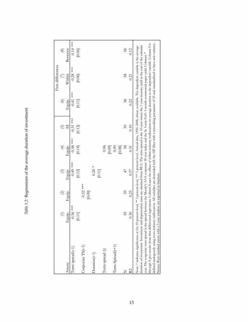
Table 1.2 reports results of regressions of Dt on the first lag of the term spread. All

of the variables in table 1.2 are standardized to have unit variance so that the regression

coefficients indicate how a one standard deviation increase in the independent variables

affects Dt in terms of its own standard deviation. The units of Dt have no deep economic

meaning on their own.

As expected, in the first column we find a highly significant negative coefficient on the

term spread and an R2 of 0.30. This is a high value; Oliner, Rudebusch, and Sichel (1995),

when forecasting the level of aggregate investment using models with as many as 11 lags

of quarterly data, obtain at best an R2 of 0.34. With a single variable, I am able to get an

R2 nearly as high for Dt. Column two uses the term spread on corporate bonds instead of

Treasuries and finds a nearly identical coefficient and R2.

The third column of table 1.2 controls for the lagged level of Dt. The coefficient is

only marginally significant and the coefficient on the term spread is essentially unchanged.

Column 4 shows that leading values of the term spread have no explanatory power for

average duration, which is consistent with the theory that firms are responding to the cost

of capital, rather than there being some underlying variable that causes the term spread

and D to generally move together.

Finally, the fifth column runs the basic regression using investment in all assets instead

12

Tabl

e1.

2:R

egre

ssio

nsof

the

aver

age

dura

tion

ofin

vest

men

t

(1)

(2)

(3)

(4)

(5)

(6)

(7)

(8)

Assets:

Equip.

Equip.

Equip.

Equip.

All

Equip.

Within

Betwee

n

Term spread

(t-1)

-0.56**

*-0.49**

*-0.58**

*-0.31**

*-0.41**

*-0.28**

*-0.14**

*

[0.11]

[0.12]

[0.14]

[0.12]

[0.11]

[0.06]

[0.06]

Corp

orate T

S(t-1)

-0.52**

*

[0.09]

Duration(t-1)

0.20*

[0.11]

Term spread

(t)

0.06

[0.09]

Term Spread

(t+1)

0.00

[0.08]

N59

59

47

58

59

58

58

58

R2

0.30

0.25

0.37

0.31

0.10

0.22

0.21

0.12

Note: * indicates significan

ce at the 10 perce

nt level, **

5 perce

nt level, **

* 1 perce

nt level. Annual data, 1950–2008, where av

ailable. The dep

enden

t variable is the av

erag

e

duration of investm

ent. Investm

ent an

d dep

reciation rates are obtained

fro

m B

EA. The term

spread

is the 10-yea

r minus the 1-yea

r trea

sury yield at the en

d of the ca

lendar

year. The co

rporate term spread

is the sp

read

betwee

n the M

oody's AAA corp

orate 30 yea

r index

and the St. L

ouis F

ed's 3 m

onth commercial pap

er yield. Columns 7

thro

ugh

9 give resu

lts from first difference

d reg

ressions. C

olumn 8 uses the effect of within-industry rea

lloca

tion on averag

e duration as the dep

enden

t variable. Column 9 is

defined

analogo

usly using cross-industry rea

lloca

tion. All variables are detrended

with the HP filter w

ith a smoothing param

eter of 25 and standardized

to hav

e unit variance

.

New

ey-W

est stan

dard errors w

ith a 3-yea

r window are rep

orted

in brack

ets.

First difference

s

13

of equipment alone. The results still go through. The symmetrical regression using only

structures investment is unenlightening because there is not enough variation in duration

within structures to provide reasonable statistical power.

To test for a break in the relationship between Dt and the term spread, I use the sup-F

test (also known as the Quandt likelihood ratio test). We might expect that the break in this

relationship would have appeared following the great moderation, when monetary policy

became more aggressive and the economy less volatile. The F-test for a break, though, is

maximized in 1958. Looking at figure 1.1, it is clear that after 1958 the volatility of Dt fell

and the volatility of the term spread rose. The F-statistic for a break is never above the

critical value reported in Andrews (1993) except for in 1958 and 1959. The highest value

outside those two years is 4.56 in 1992, well below the 10 percent critical value of 5.00.

There is thus evidence for a structural break, but not where we might have thought. For

the period since 1960, we cannot reject the hypothesis that the relationship between Dt and

the term spread has been stable.

1.4 Model

With the basic result in hand, it is useful to build a simple and stylized model to help

understand where this correlation might come from. It is tempting to immediately jump

to the conclusion that there is variation in the cost of capital (i.e. shocks to the supply of

investment goods), which drives the result in figure 1.1. The model helps identify what

other factors might induce a similar correlation.

I consider a standard infinite-horizon setup with a few simplifications for analytic

tractability. Firms face a linear production function in each type of capital, where the cur-

rent level of productivity for asset i is Bit. That is, revenue is equal to

∑i

BitKit (1.3)

where Kit is the stock of asset i at date t. Note that this revenue function ignores comple-

mentarities between types of assets. In general, if a decline in the term spread is expected

to shift investment towards long-duration assets, complementarity across assets will at-

14

tenuate this effect (in the limit of a Leontief production function, firms would never vary

the composition of the capital stock).

I follow Baxter and Crucini (1993) and Jermann (1998) in specifying the update process

for capital as

Kit+1 = (1− δi) φi (Iit−1) + φi (Iit) (1.4)

The update process for capital assumes that capital only operates for two periods for the

sake of analytic simplicity. Each asset depreciates by the factor (1− δi) between its first

and second period of operation, and is subsequently obsolete. φi incorporates adjustment

costs in investment so that a unit of investment may create less than one unit of capital. φi

takes the form

φi (Iit) =η1i

1− 1/γI1−1/γit + η2i (1.5)

φi has the useful property that the elasticity of investment with respect to Tobin’s Q will

equal the constant γ.14 The parameters η1i and η2i determine the level of investment and

the size of the adjustment costs paid and are allowed to vary across assets.15

Denoting the discount rate between dates t and t + 1 as rt+1, the firm maximizes the

discounted value of its revenue net of investment costs,

Πt = maxIit

∞

∑j=0

∑i

[exp

(−∑

jk=1rt+k

)EtBit+jKit+j − Iit+j

](1.6)

where Et denotes the expectation operator conditional on information available at date t.

All profits are discounted at the riskless rate rt.

For productivity growth, I assume that different assets may have different current lev-

els of productivity, but expected productivity growth in the future is the same for all assets,

14 This functional form has the drawback that it is not necessarily consistent with negative investment. How-ever, asset-level investment is always positive in the data, so this is not a practical concern here.

15 These two parameters allow us to choose a steady state level of investment xi where Qi = 1 and φi (xi) =xi and φ′i (xi) = 1. That is, they allow us to choose a point where the firm pays no adjustment costs overalland on the margin.

15

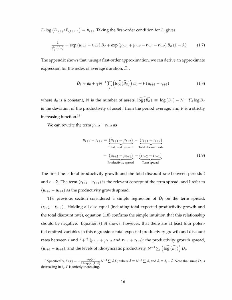
Et log(

Bi,t+j/Bi,t+j−1)= µt+j. Taking the first-order condition for Iit gives

1φ′i (Iit)

= exp (µt+1 − rt+1) Bit + exp (µt+1 + µt+2 − rt+1 − rt+2) Bit (1− δi) (1.7)

The appendix shows that, using a first-order approximation, we can derive an approximate

expression for the index of average duration, Dt,

Dt ≈ d0 + γN−1 ∑i

(log (Bit)

)Di + F (µt+2 − rt+2) (1.8)

where d0 is a constant, N is the number of assets, log (Bit) ≡ log (Bit) − N−1 ∑i log Bit

is the deviation of the productivity of asset i from the period average, and F is a strictly

increasing function.16

We can rewrite the term µt+2 − rt+2 as

µt+2 − rt+2 = (µt+1 + µt+2)︸ ︷︷ ︸Total prod. growth

− (rt+1 + rt+2)︸ ︷︷ ︸Total discount rate

+ (µt+2 − µt+1)︸ ︷︷ ︸Productivity spread

− (rt+2 − rt+1)︸ ︷︷ ︸Term spread

(1.9)

The first line is total productivity growth and the total discount rate between periods t

and t + 2. The term (rt+2 − rt+1) is the relevant concept of the term spread, and I refer to

(µt+2 − µt+1) as the productivity growth spread.

The previous section considered a simple regression of Dt on the term spread,

(rt+2 − rt+1). Holding all else equal (including total expected productivity growth and

the total discount rate), equation (1.8) confirms the simple intuition that this relationship

should be negative. Equation (1.8) shows, however, that there are at least four poten-

tial omitted variables in this regression: total expected productivity growth and discount

rates between t and t + 2 (µt+1 + µt+2 and rt+1 + rt+2); the productivity growth spread,

(µt+2 − µt+1), and the levels of idiosyncratic productivity, N−1 ∑i

(log (Bit)

)Di.

16 Specifically, F (x) = − exp(x)1+exp(x)(1−δ)

N−1 ∑i δiDi where δ ≡ N−1 ∑i δi and δi ≡ δi − δ. Note that since Di is

decreasing in δi, F is strictly increasing.

16

First, holding the term spread and the productivity spread fixed, an increase in pro-

ductivity growth (µt+1 + µt+2) or a decrease in discount rates (rt+1 + rt+2) will tilt the

distribution of investment towards long-duration assets. This effect is the primary fea-

ture of duration: long-duration assets gain more value from a decline in interest rates or

an increase in expected productivity growth than do short-duration assets. To the extent

that the term spread is correlated with long-term average productivity growth and interest

rates, then, a regression of the average duration of investment on the term spread will be

biased.

Specifically, we could spuriously find a negative relationship between the term spread

and Dt if expected long-term productivity growth is low in periods when the term spread

is high. The term spread is countercyclical, so this would correspond to a situation in

which expected long-term productivity growth (µt+1 + µt+2) is low during recessions. I

will try to control for these effects by controlling for the level of aggregate investment and

various other indicators of the state of the business cycle.

The second source of bias is that the productivity spread (µt+2 − µt+1) could be corre-

lated with the term spread. In particular, if productivity growth is expected to slow down

in the same periods that the term spread is high, we would find a spurious negative re-

lationship between average duration and the term spread. In this case, recessions would

have to be periods in which productivity growth is expected to decelerate in the future,

which seems unlikely given that recessions are periods when growth is already slow in

the first place (by definition).

Finally, the levels of productivity across assets could be related to duration, affecting

Dt through the N−1 ∑i

(log (Bit)

)Di term, which can be thought of as the covariance be-

tween duration and productivity across assets. If this covariance changes over time and is

systematically related to the level of the term spread, then omitting it from the regression

would bias the coefficient on the term spread.

Over long horizons, investment and productivity shift substantially across different

assets. The most notable of these changes is the long-run decline in prices and increase

17

in investment in computers and software (Tevlin and Whelan, 2003).17 The model would

interpret this phenomenon as an increase in Bit for low-duration assets, which drives Dt

downward. A simple way to control for those movements is to detrend Dt.

Short-run movements in idiosyncratic productivity are more difficult to account for,

though. If changes in the term spread are correlated with shifts in productivity that favor

certain assets, then the regression of Dt on the term spread will be biased. In the empirical

analysis below, I discuss and control for some specific mechanisms, most importantly in-

dustry demand shifts, that could drive high-frequency movements in N−1 ∑i

(log (Bit)

)Di.

Instead of running a regression of average duration on investment, it would be nice

to estimate a more fundamental parameter, such as the coefficient on marginal Q, which

tells us about the size of adjustment costs in investment. One way to do that would be to

calculate Tobin’s Q for each asset individually, as in Abel and Blanchard (1986), using the

full term structure of interest rates. The problem is that we do not actually directly measure

the marginal product of any individual asset at any point in time. Moreover, we do not

measure anything like the true discount rate for each asset. Rather, the term spread in

this paper is measured using Treasury yields and is taken as an indicator of differences in

discount rates across assets. A deeper problem is that Abel and Blanchard’s method would

also require forecasting inflation at very long horizons, when the literature generally finds

that inflation is difficult to forecast even at quarterly and annual horizons (e.g. Atkeson

and Ohanian, 2001).18

17 See also Caballero, 1994, and Schaller, 2006, for studies of the relationship between investment and thecost of capital in the long-run.

18 Euler equation estimation is also an option. In a pair of papers, Oliner, Rudebusch, and Sichel (1995, 1996)study the effectiveness and internal consistency of Euler equation models for investment. They obtain param-eter estimates that are somewhat difficult to reconcile with economic theory, find that supposedly "structural"parameters are unstable over time, and that the models have little forecasting power. There are also legitimateconcerns about the validity and relevance of the instruments used in these models (especially when extendedto asset-level data).

I attempted to estimate an Euler equation using the panel of data on asset-level investment. Between two-stage least squares, LIML, and GMM methods, there were substantial differences in results indicating thatthe model is misspecified or there are problems with the instruments. I also replicated some of the troublingresults found by Oliner, Rudebusch, and Sichel. Furthermore, Euler equations are clearly difficult to estimateeven with quarterly data, and I only have annual data on asset-level investment.

The Euler-equation method is also more restrictive than the methods used in this paper because it is difficultor impossible to incorporate all of the controls that I consider. Euler equations are useful for estimating specificparameters in tightly theorized models. The regressions used here are meant to test a broader range of possibleexplanations for the correlation between average duration and the term spread and to measure the explanatory

18

What the regression of average duration on the term spread is useful for is testing

whether the term spread drives investment in the direction that we would expect and

how much explanatory power the term spread has for the cross-section of investment. A

high R2 in a regression of average duration on the term spread is evidence that the cross-

section of interest rates is an important determinant of the cross-sectional distribution of

investment.

1.5 Alternative explanations

The working hypothesis is that the negative relationship between average duration

and the term spread is a simple cost-of-capital effect. The model in the previous section

shows that there are a number of other factors that could cause us to find the correlation we

observe in figure 1.1. This section considers a range of possible alternative explanations.

I find that the correlation is driven to some extent by these other factors, but that the cost

of capital retains a substantial amount of explanatory power and is generally the most

powerful variable for explaining average duration.

1.5.1 Correlations by asset and industry

One possible explanation for the correlation between the term spread and D is that

demand for the products of different industries depends on the term spread. For exam-

ple, suppose when the term spread is high consumers demand fewer durable goods (the

term spread tends to be countercyclical, as are durables purchases; Yogo, 2006). If durable

goods industries tend to use relatively more long-duration capital than services providers

(for example, a car manufacturer may use more heavy machinery than a barber shop), then

we would see investment shift towards low-duration assets. In the terms of the model, this

is a story about the covariance term ∑i D (δi)[log (Bi0)− N−1∑i log (Bi0)

]. The correlation

between D and the term spread then would be driven by consumer demand (and hence

the variation in the marginal product across assets) instead of the cost of capital. We can

power of the term spread. I therefore leave the Euler equation analysis of this panel dataset for future work.

19

test this hypothesis by decomposing D into components driven by within-industry reallo-

cation and changes in the composition of investment across industries.

As noted above, the BEA not only reports data on aggregate investment; it also gives

levels of investment at the asset×industry level. Denoting the first difference of Dt as ∆Dt,

we can decompose ∆Dt following van Ark and Inklaar (2006) using the industry-level data

as

∆Dt = ∑j

[12

(Ij,t

It−

Ij,t−1

It−1

) (Dj,t + Dj,t−1

)]+ ∑

j

[12

(Ij,t

It+

Ij,t−1

It−1

) (Dj,t − Dj,t−1

)](1.10)

where Dj,t ≡ ∑iIj,i,t

Ij,tDi is the average duration of industry j at time t. The first part of

equation (1.10) can be thought of as a cross-industry reallocation effect. It sums the changes

in the industry investment shares weighting by their average depreciation rates at dates

t and t − 1. The second term is the within-industry reallocation term. It represents the

effects of industries changing their mix of investment among different assets. I refer to the

two effects as the between and within-industry effects, respectively.

The final three columns of table 1.2 report results from first-differenced regressions

of ∆D and its decomposition (1.10) on the change in the term spread. ∆D and ∆TS are

standardized to have unit variance as in the remainder of the table. The three columns

report results from regressions with different dependent variables. The first column uses

∆D. The coefficient on the term spread is similar to though somewhat smaller than the

coefficient in column 1. In other words, the relationship between D and the term spread

is somewhat weaker in high frequency data, which is perhaps not surprising considering

the effects of planning, ordering, and building lags. The coefficients in columns 7 and 8

by definition sum to the coefficient in column 6. The within-industry coefficient is twice

the size of the between-industry coefficient; in other words, two thirds of the aggregate

effect comes from reallocation within industries. The hypothesis that industry demand is

correlated with the term spread seems to be true, but it explains only a minority of the

variation in average duration over time.

20

To analyze how the relationship in figure 1.1 and table 1.2 differs across assets, I run a

regression of each asset’s share of aggregate investment on the term spread.19 Specifically,

for each asset we run the regression

Iit

∑i Iit= αi + βiTSt + ε it (1.11)

It is straightforward to show that if βi is negatively related to each asset’s duration, then

there will be a negative relationship between the term spread and Dt. This is a way of ask-

ing whether the relationship we observe at the aggregate level is pervasive across assets,

or is driven by a few outlier assets.

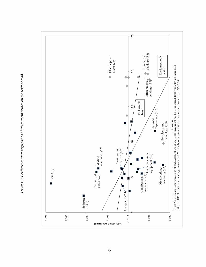
Figure 1.4 plots the coefficients βi against duration. The black boxes are for equipment,

grey diamonds structures. Regression lines are included for the sample of all assets and

for equipment only. The correlations between βi and Di are -0.42 and -0.31 for equipment

only and all assets, respectively. Looking across equipment, the relationship between the

composition of investment and the term spread is broadly based not driven by a few out-

liers.

The plot includes labels for the assets that make up the largest part of investment over

the last 15 years. Numbers in parentheses represent their percentage shares over that pe-

riod. Within equipment, auto purchases as a share of total investment are far more pos-

itively correlated with the term spread than any other asset, though they represent a rel-

atively small part of aggregate investment. Software is the single largest component of

investment and it is well above the best fit line. Communication equipment and comput-

ers are next in the rankings and are somewhat closer to the regression line.

Structures do not match the results for equipment very well. While the shares of struc-

tures are generally negatively related to the term spread, they are not as negative as we

would think from just looking at equipment. Electric-power plants, in particular, are a

large positive outlier. As noted above, the fact that building lags average over a year (a

time that does not take into account the time required for planning) is likely to distort the

19 To control for long-term changes in the composition of investment I first detrend the dependent variableand the term spread using the HP filter with a smoothing parameter of 25 as above.

21

Figu

re1.

4:C

oeffi

cien

tsfr

omre

gres

sion

sof

inve

stm

ents

hare

son

the

term

spre

ad

0.00

1

0.00

2

0.00

3

0.00

4Regression Coefficient

Electric power

plants (2.0)

Cars (3.4)

Software

(14.9)

Medical

equipment (3.7)

Trucks and

buses(6.9)

Furniture and

fixtures (3.3)

-0.002

-0.001

-1E-17

05

10

15

20

25

Duration

Equipment only

best fit

Full sample

best fit

Computers (7.4)

Metalworking

machinery (2.6)

Petroleum

and

natural gas (4.0)

Railroad

Equipment(0.6)

Commercial

build

ings (5.3)

Communication

equipment (8.2)

Office/medical

build

ings

(4.3)

fixtures (3.3)

Construction

machinery (2.1)

Note: C

oefficients from

regressions of each asset's share of aggregate investment on the term

spread. B

oth variables are detrended

with the HP filter with a smoothing param

eter of 25. N

umbers in parentheses are investment shares over 19

93–20

08.

22

regressions for structures.

1.5.2 The business cycle, volatility, and other explanations

Table 1.3 explores a number of other mechanisms that could cause the observed cor-

relation beyond changes in demand across industries. Columns 1 and 2 control for the

business cycle with the lagged detrended unemployment rate and level of output. In both

cases the coefficient on the term spread is smaller but still statistically and economically

significant. This is perhaps not surprising: even if the term spread does represent a true

cost-of-capital effect, it is also a proxy for the business cycle. Controlling for other business

cycle indicators will probably lower its coefficient. Including the current value and longer

lags of unemployment and output do not change the results of the regressions.

Another obvious question is whether there is a mechanical relationship between aver-

age duration and the level of investment. Suppose a firm has equal stocks of two assets,

one with a depreciation rate of 1 percent, the other 10 percent. In a maintenance phase

with no net capital growth, there will be 10 times as much investment in the high depreci-

ation as the low depreciation asset. However, in an expansion phase, assuming both assets

are expanded equally, investment will shift towards being equally balanced between the

two assets. If the term spread is correlated with the level of investment, it might also

then be correlated with average duration. Column 3 tests that hypothesis by including

detrended aggregate equipment investment. Puzzlingly, unlike the example just given,

when investment is high, duration actually tends to be low. However, the coefficient on

the term spread is still large and significant. The term spread thus has explanatory power

beyond its indication of either the business cycle of overall level of investment. Column 4

shows that if we include all three aggregate indicators, unemployment, GDP, and invest-

ment, the coefficient on the term spread is the highest, and has the highest t-statistic, of

any of the variables (implying that the marginal R2 of the term spread is higher than any

of the business-cycle indicators).

Abel et al. (1996), among many others, study the effects of irreversibility on investment.

With irreversibility, when idiosyncratic uncertainty is high, firms may be less willing to

23

Tabl

e1.

3:R

obus

tnes

ste

sts

(1)

(2)

(3)

(4)

(5)

(6)

(7)

Term Spread

(t-1)

-0.27**

-0.33**

*-0.65

***

-0.44**

*-0.41**

*-0.36**

*-0.37**

*

[0.12]

[0.11]

[0.11]

[0.08]

[0.09]

[0.10]

[0.10]

Unem

ploym

ent(t-1)

-0.45**

*-0.01

[0.14]

[0.19]

GDP(t-1)

0.38

***

0.40

**0.37

***

0.31

**0.38

***

[0.10]

[0.17]

[0.12]

[0.14]

[0.09]

Inve

stmen

t(t)

-0.23**

-0.29**

*

[0.11]

[0.09]

SD_pro

fits(t+1)

-0.01

[0.09]

SD_return

s(t+

1)-0.31**

*

[0.08]

Ban

k tigh

tness(t)

-0.24**

*

[0.08]

Value sp

read

(t)

-0.22**

*

[0.07]

N58

5959

5844

3759

R2

0.45

0.45

0.35

0.52

0.65

0.62

0.49

Note: S

ee tab

le 2. T

he dep

enden

t va

riab

le is the detrended

ave

rage

duration of eq

uipmen

t inve

stmen

t. T

he va

lue sp

read

is the ga

p between log book/

marke

t

(B/M) for the top and bottom 30 percent of firm

s ranke

d by B/M, a

mong the sm

aller 50

percent of firm

s, m

easu

red at the beg

inning of the year. S

D_pro

fits and

SD_return

s are the cross-sectional standard dev

iations of quarterly firm

pro

fit growth and stock

return

s, controlling for a time tren

d and 3-digit industry dummies.

The unem

ploym

ent rate is the national rate obtained

fro

m the BLS. G

DP is real G

DP fro

m the BEA. Ban

k tigh

ness is the Fed

's Survey of Sen

ior Loan

Officers

index

(from M

organ

and Lown, 2

006). Inve

stmen

t is agg

rega

te real nonresiden

tial equipmen

t inve

stmen

t. All va

riab

les are detrended

with the HP filter w

ith a

smoothing param

eter of 25

(ex

cept for the va

lue sp

read

, for which it is 100

), and standardized

to hav

e unit variance.

24

invest in long-duration assets. Intuitively, if it is more difficult to sell a long-duration

asset (e.g. a large wind turbine) because it is more costly to disassemble than a short-

duration investment, then there is option value to delaying investment which is increasing

in uncertainty.20 Campbell et al. (2001) and Bloom (2009) find that when the volatility of

returns on the aggregate stock market is high, so is idiosyncratic firm volatility. If the term

spread is partially driven by aggregate volatility (a finding of Bloom, 2009, and implied by

many term structure models, e.g. Longstaff and Schwartz, 1992), and volatility drives D,

then we would find a spurious correlation between the term spread and D.

I use two measures of cross-sectional volatility that are also used in Bloom (2009): the

period-by-period cross-sectional standard deviations of firm quarterly profit growth and

stock returns, including controls for 3-digit SIC industries.21 Column 5 of table 1.3 reports

results of a regression of D on the volatility indexes. Both measures of volatility are posi-

tively correlated with the next year’s term spread, which is consistent with Bloom’s (2009)

results. He finds that volatility shocks lead to economic contractions and reductions in the

short rate. Table 1.3 shows that conditional on the term spread and the state of the busi-

ness cycle, high stock return volatility (though not profit growth volatility) in the follow-

ing year is associated with low duration investment. This is consistent with the hypothesis

that long-duration investment involves a bigger commitment for firms than short-duration

investment. That is, the hypothesis that high volatility interacts with fixed costs of adjust-

ment to decrease investment seems to apply more strongly to long than short-term assets.

Note, though, that even when controlling for volatility, the term spread remains significant

and has a large coefficient.

Another alternative hypothesis is that the term spread does not reflect the cost of capital

but is simply an indicator of the stance of monetary policy. When the Federal Reserve

contracts the money supply, this may inhibit bank lending, as in Kashyap and Stein (2000).

If banks are more likely to finance projects of a certain duration (either high or low), then

the term spread might simply be correlated with movements in D because it is correlated

20 House and Shapiro, 2008, discuss the relationship between real option-type effects and asset duration.

21 The original data was retrieved from Compustat and CRSP. I obtained the data used here from NickBloom’s website.

25

with bank lending standards. One way to test this hypothesis is to try to directly measure

bank lending standards. The Federal Reserve has administered a Survey of Senior Loan

Officers since 1967 (with a gap between 1983 and 1989) that asks banks about the level of

their lending standards.22 Column 6 includes the tightness index from this survey in the

regression. The coefficient on the term spread remains significant. When bank lending

standards are relatively tight (a high value of the index), average duration is low. This is

perhaps surprising, since banks are usually thought of as financing short-duration projects,

while firms go to credit markets for longer-term financing. One possible explanation is

that lending standards tend to be high when other factors are driving firms towards short-

duration investment. In particular, standards might be high in times of high uncertainty.

The appendix includes further robustness tests. When all of the controls are included

simultaneously, the term spread is the only significant variable and it has more explanatory

power than any of the other variables individually.

Lettau and Wachter (2007) argue that the differences in returns between high and low

book/market (B/M) stocks can be explained by differences in the duration of their cash

flows (see also Hansen, Heaton, and Li, 2008). A high value spread is associated with

a high valuation for growth stocks, or long-duration assets, which implies investment

in long-duration assets should be high. Since stock prices represent claims on capital,

whereas Treasury bonds are claims on currency, we might expect that the value spread

would have more predictive power than the term spread. Column 7 of table 1.3 reports

the results of a regression including the value spread. I measure the value spread here as

the ratio of the book to market ratios for the top and bottom third of stocks sorted by book

to market (as reported on Kenneth French’s website).23 The coefficient is significantly neg-

ative: the opposite of what the duration theory of the value spread would predict. One

possible explanation for this result is that firms with growth stocks tend to have lower-

duration assets—e.g. technology firms—so when their values are high average duration

22 I obtain data from Lown and Morgan, 2006.

23 Specifically, French reports value spreads for small and large stocks, split at the median of market capital-ization. I average these two value spreads. Furthermore, I detrend the value spread using the HP filter with asmoothing parameter of 100.

26

falls. To many readers, that may have been the obvious result all along. Nevertheless, it

runs against Lettau and Wachter’s theory.

1.6 Consumer durables

If the term spread truly represents a cost of capital effect then we would expect house-

hold purchases of durable goods to respond to it in a manner similar to nonresidential

investment. Households face some of the same choices as firms when deciding what types

of durable goods to purchase. In particular, long-lasting durable goods may have financ-

ing arrangements with longer terms than those of shorter duration assets.24

Denoting the duration of durable good of type i as Ci and purchases as Pi, I define the

average duration of consumer durables purchases as

Ct ≡∑i CiPit

∑i Pit(1.12)

Table 1.4 lists the assets available from the BEA, along with their depreciation rates and

durations. The two assets with the lowest depreciation rates are luggage and furniture at

13 percent. Computer software and motor vehicle parts have the highest rates at 76 and

90 percent, respectively. The assets are mostly clustered in a small range of depreciation

rates, though: three fourths have depreciation rates between 16 and 25 percent.

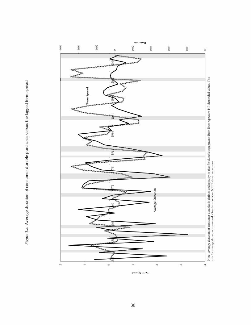
Figure 1.5 plots HP-detrended Ct against the detrended term spread. As in figure 1.1,

the axis for Ct is reversed so that a negative correlation in the data is an easier-to-read posi-

tive correlation in the figure. For most of the sample, there is a strong negative correlation,

just as we observe for nonresidential investment. In a regression similar to those in table

1.2, consumer durables on the lagged term spread, the coefficient is -0.31 with a p-value of

0.008. There is thus a significant relationship over the full sample, though the correlation is

somewhat weaker than what we observe for nonresidential investment. The correlation is

clearest between 1965 and 1991. For nonresidential investment the correlation is more con-

sistent over time, which explains why the QLR test in section 1.3 indicated a break point

24 Attanasio, Goldberg, and Kyriazidou (2008) show that auto loan terms tend to be between three and fiveyears, while home loans may be as long as 30 years.

27

Table 1.4: Consumer durables, depreciation rates, and durations

Depreciation

rate (percent)

Duration

(years)

Asset

Motor vehicles and parts

0.28 3.27 Autos

0.25 3.70 Light trucks

0.90 1.11 Motor vechicle parts & accessories

Furnishings and household equipment

0.13 6.63 Furniture

0.18 4.90 Clocks, lamps, lighting fix & other

0.18 4.91 Carpets and other floor coverings

0.18 4.89 Window coverings

0.16 5.37 Household appliances

0.18 4.90 Glassware, tableware, & household uten

0.18 4.90 Tools & equipment for house & garden

Recreational goods and Vehicles

0.20 4.45 Video & audio equipment

0.18 4.92 Photographic equipment

0.44 2.21 Personal computers and peripheral equip

0.76 1.31 Computer software & accessories

0.18 4.91 Calcs, typewrtrs, & oth info proc equip

0.18 4.91 Sporting equip, supplies, guns, & ammo

0.18 4.91 Motorcycles

0.18 4.92 Bicycles & accessories

0.18 4.90 Pleasure boats

0.18 4.91 Pleasure aircraft

0.26 3.52 Other recreational vehicles

0.18 4.91 Recreational books

0.20 4.46 Musical instruments

Other durable goods

0.16 5.36 Jewelry & watches

0.32 2.95 Therapeutic appliances & equip

0.18 4.91 Educational books

0.13 6.63 Luggage & similar personal items

0.18 4.88 Telephone & facsimile equipmentNote: Depreciation rates are otained from the BEA. Duration is measured as 1.03/(0.03+δ).

28

only in the very beginning of the sample.

The relationship between Ct and the term spread seems to abruptly break down after

1991. If we run a QLR test as before, we can reject the hypothesis of no break at the 1

percent level. The F-statistic is maximized in 1991, only one year different from the local

maximum that is obtained in the F-statistic for nonresidential investment.25 The fact that

these two break tests are maximized around the same time suggests that the breakdown

in the consumer durables plot is not due to a factor that is specific to consumers.

One possible consumer-specific explanation is that there was some sort of change in

consumer credit markets around 1991. Perhaps easier access to credit cards made con-

sumers less dependent on long-term financing for some durables purchases, which made

them less sensitive to long-term credit conditions. The Flow of Funds accounts measure

total credit card balances and household net worth. The ratio of consumer credit debt to

net worth rises from 1.0 to 3.8 percent between 1945 and 1965, but then stays flat subse-

quently. While there were certainly changes in consumer credit markets following 1965,

the total quantity of credit has remained in this sense stable.

1.7 The firm-level mechanism

To augment the analysis above, this section studies two aspects of firm-level invest-

ment. I begin by asking whether firms that invest in long-duration assets also tend to sell

long-term debt. Next, I look at whether industries with larger cash holdings are more

sensitive to the term spread. The data answer both these questions in the affirmative, but

when we include a full set of industry and year dummies the results go away, possibly

because of insufficient statistical power. The first result indicates that when firms go to

debt markets, the interest rate that they face depends on the duration of the investment

they plan on undertaking. The second result shows that firms that are more likely to have

to go to debt markets seem to vary the composition of their investment more strongly in

response to interest rates.

25 Note, again, that the local maximum for nonresidential investment is not statistically significant.

29

Figu

re1.

5:A

vera

gedu

rati

onof

cons

umer

dura

ble

purc

hase

sve

rsus

the

lagg

edte

rmsp

read

-0.06

-0.04

-0.02

0 0.02

0.04

-1012

1951

1956

1961

1966

1971

1976

1981

1986

1991

1996

2001

2006

Duration

Term Spread

Term Spread

Average Duration

0.06

0.08

0.1

-4-3-2Average Duration

Note: Average duration of consumer durables is defined analogously to that for durable equipment. Both lines represent HP-detrended values. The

axis for average duration is reversed. Grey bars indicate NBER-dated recessions.

30

1.7.1 The maturity of assets and debt

The link between the term spread and the cost of capital will be most clear to managers

if investment in long-duration assets is financed with long-duration debt. If, for example,

firms always borrow at the same maturity and simply roll over their debt, then they might

only pay attention to the interest rate for the maturity at which they borrow, instead of the

full term structure.

Baker, Greenwood, and Wurgler (BGW, 2003) find that firms time the debt market when

they sell bonds. In particular, when the term spread is high firms sell short-term debt.

BGW argue that firms do this because when the term spread is high, the prices of short-

term bonds are expected to fall in the future. Firms are selling expensive or overpriced

debt, which BGW claim represents arbitrage.

But if it is true that firms try to match the maturity of their debt to the maturity of their

investments, then the results in the previous sections could explain the BGW result. Match-

ing the maturity of debt to assets reduces potential deadweight losses from bankruptcy

(see, e.g., Stohs and Mauer, 1996). Graham and Harvey (2002) report evidence from sur-

veys that maturity matching is the single most important determinant of debt maturity

choice.26

Section 1.3 showed that when short-term yields are low, firms invest in short-duration

assets. If the maturity-matching hypothesis is correct then those firms should also sell

short-duration debt. That matches the Baker et al. result: low short yields are associ-

ated with short-duration investment, which is associated with sales of short-duration debt.

BGW claim that firms are arbitraging debt markets; I claim they are managing risk through

maturity-matching. The key to completing the argument is showing that firms actually do

try to match the duration of their debt to that of their assets. In this section I provide

evidence in support of this proposition.27

26 See also Barclay and Smith, 1995, and Guedes and Opler, 1996, among many others.

27 Baker at al. tried measuring the duration of assets with a similar strategy to mine. However, rather thanusing industry depreciation reported by the BEA, they used the amount of depreciation reported to the IRSby individual firms. Presumably this data was substantially more noisy than the BEA data, which causedthem to find inconclusive results. Moreover, accounting depreciation is in general not the same as economicdepreciation. The majority of firms use straight line depreciation, rather than the declining balance methodfound to better match the resale value of assets (Hulten and Wykoff, 1981).

31

I obtain data from two sources. Data on capital stocks come from the BEA’s detailed

fixed asset tables as before.28 I continue to measure average duration within industry j as

Djt =∑i Di Iijt

∑i Iijt(1.13)

where i indexes assets, j indexes industries, and I is investment

I obtain data on corporate debt from Compustat. Following Baker et al. (2003) and

Greenwood et al. (2009), the long-term share in a given industry and year is the sum of

all outstanding long-term debt reported by firms in that industry divided by all long and

short-term debt.29 I estimate issuance of long-term debt as the change in the level of long-

term debt, and short-term issuance as simply the level of short-term debt (since short-term

debt has, by definition, a maturity of less than one year). The long-term issuance share is

then just the ratio of long-term issuance to total issuance.30

An important issue here is that Compustat only covers publicly traded firms, whereas

the BEA’s fixed-asset data covers all firms. To the extent that private firms have limited

access to long-term credit markets, this will bias the level of the long-term share up-

wards.31 It is less clear, though, that selection should cause us to spuriously find that

high-depreciation industries have a low long-term share. The selection would need to oc-

cur in such a way that firms in high-depreciation industries are more likely to go public

but are no more likely to have access to long-term credit markets.

Table 1.5 reports regressions of the long-term level and issuance shares on industry

average duration. The first two columns use the level share, the second two the issue share.

Columns 2 and 4 include industry fixed effects. Each regression includes year dummies

and the standard errors are corrected for clustering within industries. Columns 1 and 3

28 The BEA has its own industry classification which is slightly different from NAICS. I use industries thatroughly correspond to a 2-digit NAICS classification, but I combine some industries to ensure that I havesufficient firm observations to get good financial data. I end up with 22 industries

29 I measure long term debt as the sum of items 9 (long term borrowing) and 44 (long term debt about toretire), and short term debt as item 9 plus item 34 (current liabilities) minus long term debt.

30 I drop firm observations if the level of long term debt drops by more than one half (as this amount ofretirement is implausible). Industry-year observations are dropped if they have a negative level of long termdebt issuance.

31 For example, Titman and Wessels, 1988, find that small firms are less likely to use long-term debt financing.

32

show that there is a significant negative relationship between long-term debt levels and

issuance and the depreciation rate of assets in an industry. However, columns 2 and 4

show that when we include industry dummies the effect goes away. That is, there is not

evidence that when an industry shifts towards higher-depreciation assets, it also changes

the composition of its debt.

One reason I do not find within industry effects in table 1.5 could be that the data is not

sufficiently precise. The median number of firms that is used to create the industry×year

observations is only 148, and the 25th percentile is 30. Moreover, the measure of the du-

ration of debt is extremely rough. Firms could easily be changing the maturity of their

long-term issues, rather than substituting between long and short-term issues.32

1.7.2 Cash reserves and investment

If firms match the maturities of assets and debt, as suggested by table 1.5, then when

they borrow to finance investment, shifts in the term spread directly feed into their cost of

capital, and presumably their investment decisions. However, when firms finance invest-

ment internally, we might think they simply use a rule-of-thumb method for the cost of

capital, ignoring the term structure of interest rates (e.g. Graham and Harvey, 2002).

I study this question by looking at how investment differs across industries with dif-

ferent cash holdings. I study the following regression

Dj,t = αj + β1TSt−1 + β2CHj,t + β3TSt−1 × CHj,t + ε j,t (1.14)

where, as before, TSt is the term spread and CHj,t is a measure of cash holdings in industry

j at time t. The coefficient β3 measures the effect of cash holdings on the response of an

industry’s average duration of investment to the term spread. Under the hypothesis that

firms that can finance investment internally respond less to the term spread, we should

observe a positive value for β3.

I use two measures of an industry’s ability to finance investment internally: its total

32 While there is data with more detail on the duration of corporate debt, it does not have a long enoughtime series to be useful for finding the aggregate effects that I am looking for here.

33

Table 1.5: Regressions of the long-term corporate level and issues shares

(1) (2) (3) (4)

Levels Levels Issues Issues

Duration 0.013 *** -0.008 0.021 ** -0.008

[0.005] [0.006] [0.11] [0.012]

Fixed Effects? No Yes No Yes

N 1,040 1,040 1,023 1,023Note: The long term level share is the share of total corporate debt accounted for by long term (>1 year

maturity) debt. The issues share is the share of issues accounted for by long term debt. Duration is the

average duration rate of the industry's capital stock. All regressions include year dummies. Standard

errors reported in brackets are corrected for clustering within industries. Annual data for 22 industries,

1950–2008.

34

current cash holdings and its cash flows (income before extraordinary items), both scaled

by current property, plants, and equipment (PPE).33 One of the measures for CHj,t is a

flow, while the other is a stock. If industries differ in the amount of cash that they prefer to

hold at any given time, then cash flows might be more relevant for their ability to finance

investment internally. On the other hand, cash reserves could be saved precisely for use

in future investment, and hence represent a source of funds for investment.34 I test both

possibilities.

As above, I obtain data from Compustat and detrend Dj,t and TSt with the HP filter. I

subtract industry means from the measure of cash holdings, CHj,t, so that the coefficient

on the interaction term, β3, represents the change in the response of Dj,t to the term spread

depending on the difference between the industry’s current cash holdings and the sample

average for that industry.

Columns 1 and 2 of table 1.6 report estimates of equation (1.14). Column 1 shows

that cash flows seem to have no significant relationship with the response of Dj,t to the

term spread. In column 2 we see, though, that cash holdings have a strong effect. For an

industry with its sample average of level of cash holdings, the response of D falls by 0.15

standard deviations for every one standard deviation increase in the term spread. For an

industry with cash holdings one standard deviation above their mean, this response falls

to only 0.08 standard deviations. This result fits with the hypothesis that when firms are

forced to finance investment in credit markets they are more sensitive to the cost of capital.

Columns 3 and 4 are the same as columns 1 and 2 except that I generate a variable

CH j,t, by regressing CHj,t on a set of year and industry dummies. CH j,t thus measures the

deviation of an industry’s cash holdings relative to both its sample average and the average

for the year. This controls for general trends in cash holdings over time. The coefficients

on the interaction terms are no longer significant. As before, this may simply be a power

issue. Note that the standard error on the interaction term is substantially larger in column

33 The results are unchanged if we use free cash flow instead of income.

34 See Opler et al., 1999, for an analysis of the determinants of cash holdings and their use for investment, andthe large literature following Fazzari, Hubbard, and Petersen, 1988, on the relationship between investmentand cash flows.

35

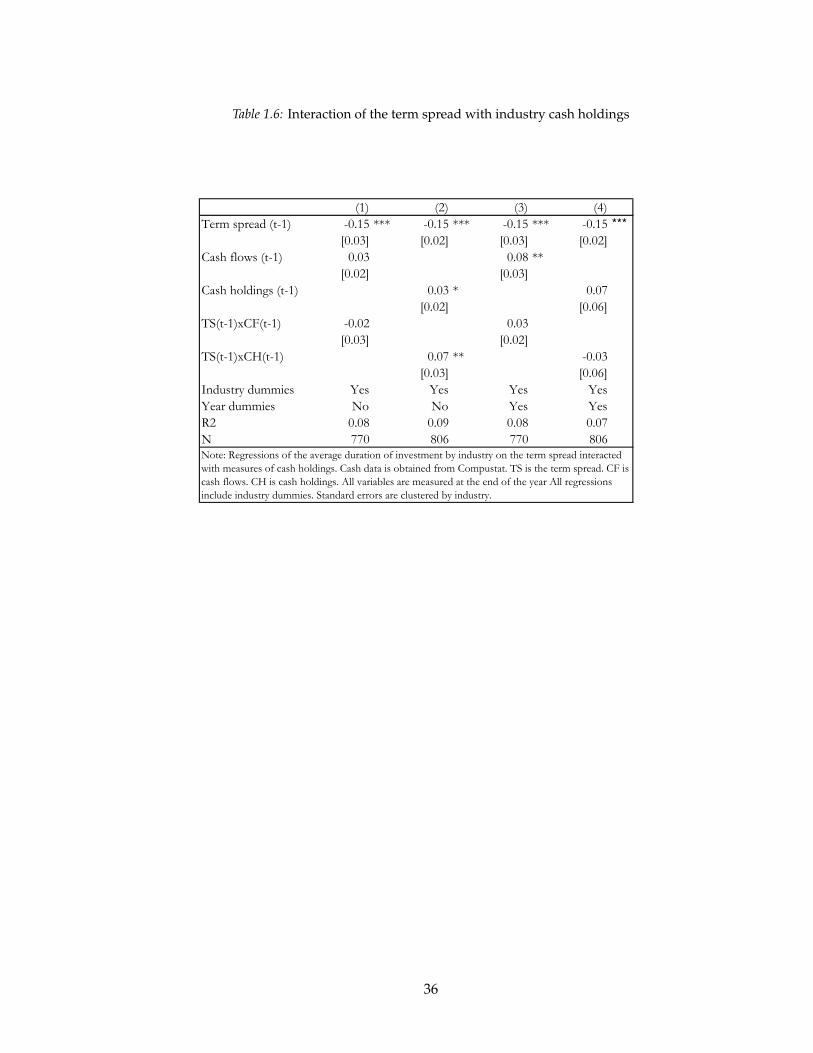
Table 1.6: Interaction of the term spread with industry cash holdings

(1) (2) (3) (4)

Term spread (t-1) -0.15 *** -0.15 *** -0.15 *** -0.15 ***

[0.03] [0.02] [0.03] [0.02]

Cash flows (t-1) 0.03 0.08 **

[0.02] [0.03]

Cash holdings (t-1) 0.03 * 0.07

[0.02] [0.06]

TS(t-1)xCF(t-1) -0.02 0.03

[0.03] [0.02]

TS(t-1)xCH(t-1) 0.07 ** -0.03

[0.03] [0.06]

Industry dummies Yes Yes Yes Yes

Year dummies No No Yes Yes

R2 0.08 0.09 0.08 0.07

N 770 806 770 806Note: Regressions of the average duration of investment by industry on the term spread interacted

with measures of cash holdings. Cash data is obtained from Compustat. TS is the term spread. CF is

cash flows. CH is cash holdings. All variables are measured at the end of the year All regressions

include industry dummies. Standard errors are clustered by industry.

36

4 than column 2. We in fact cannot reject that the two coefficients are equal.

1.8 Conclusion

This paper shows that there is a strong relationship in aggregate data between invest-

ment and the cost of capital. I find that the term spread can explain a third of the variation

of the cross section of investment. While this relationship does not quantify the magni-

tude of internal adjustment costs facing firms, it does show that the cost of capital is a

major factor driving the variation in the type of investment that firms do. The composition

of investment changes meaningfully over the business cycle, and a substantial portion of

these changes can be explained by the term spread alone.

The results are robust to including a variety of controls, including multiple indicators

of the state of the business cycle. None of the controls eliminate the coefficient on the term

spread. Moreover, when we include all of the controls at once, the term spread is the only

variable that remains significant. Of all of the variables I study, the term spread is the most

robust and powerful explanator of the distribution of investment. The dimension of in-

vestment studied here has not been examined before. The results extend also to consumer

durables purchases: households tend to buy less-durable durables when the yield curve is

steep.

Cochrane (2011) gives an extensive review of the literature on return predictability and

variation in the price of risk, arguing that shifts in discount rates are part of "the central

organizing question of asset pricing research." As Treasury bonds have (nominally) risk-

less payoffs, shifts in the term spread are purely driven by discount rates. The finding that

the term spread determines the composition of investment is thus connected to Cochrane’s

organizing question by showing its relevance for the aggregate economy, and not just fi-

nancial markets.

There are many other cross-sectional sources of variation in the cost of capital beyond

differences in asset lives. Tax policies, e.g. R&D tax credits and bonus depreciation, distort

the cost of capital, as will changes in the price of risk. The finding here that shifts in the

term structure of interest rates affect the composition suggests that tax policy can succeed

37

distorting investment choices. Similarly, to the extent that the price of risk varies over time,

an interesting question is whether a high price of risk causes businesses to shift relatively

towards low-risk/low-reward projects.

38

2. A MODEL OF TIME-VARYING RISK PREMIA WITH HABITS AND PRODUCTION

2.1 Introduction

Stock prices are more volatile than can be explained by movements in expected divi-

dends. Moreover, excess returns on the aggregate stock market are predictable over time.

The two phenomena are connected: changes in the discount rates applied to future divi-

dends can induce excess volatility in asset prices. This paper develops a new preference

specification with time-varying risk aversion that generates realistically predictable and

volatile stock returns. When combined with a production framework, the model can match

the short and long-run volatilities of output, consumption, and investment growth and at

the same time generate a high and volatile price of risk. Simulated stock-return forecast-

ing regressions are consistent with empirical results, and the model also delivers a new

method for forecasting stock returns. The structural estimate of risk aversion has an R2 for

5-year stock returns in the post-war period of over 50 percent.

The standard model of time-varying risk aversion is the habit specification of Camp-

bell and Cochrane (1999).1 In their model, when an agent’s consumption falls close to

her habit, her risk aversion rises. Using aggregate consumption data, they find that their

implied risk aversion measure can explain a large proportion of the movements in the

price-dividend ratio on the stock market. Campbell and Cochrane study an endowment

economy, though, so they never test whether their utility function generates a realistic

consumption process in equilibrium. In fact, Lettau and Uhlig (2000) and Rudebusch and

Swanson (2008) find that Campbell–Cochrane preferences imply that consumers smooth

1 A partial selection of other early papers studying habit formation is Abel (1990), Constantinides (1990),Boldrin, Christiano, and Fisher (2001) and Jermann (1998).

For other papers that study return predictability in a production setting, see Gourio (2010), Campanale,Castro, and Clementi (2010), and Guvenen (2009), though note that the latter two papers do not match thedegree of predictability observed in the data.

39

consumption growth extremely and implausibly strongly following technology shocks in

standard general-equilibrium models.

This paper embeds the intuition behind Campbell and Cochrane (1999)—that persis-

tent external habits can induce time-varying risk aversion—into the framework devel-

oped by Kreps and Porteus (1978), Epstein and Zin (1989), and Weil (1989). The Epstein–

Zin specification allows us to model risk aversion and intertemporal substitution sepa-

rately, while the Campbell–Cochrane intuition motivates time-variation in risk aversion.

In particular, consumers are modeled as having a time-varying external habit, which is

a benchmark to which they compare their own lifetime utility. When lifetime utility is

farther above the benchmark, risk aversion over proportional shocks to future welfare is

lower. By explicitly separating variation in risk aversion from intertemporal substitution,

the Epstein–Zin framework eliminates the problems that arise when standard Campbell–

Cochrane preferences are used in a production setting. I refer to the new preference speci-

fication as the EZ-habit model for its combination of these two frameworks.2

The simple real business cycle (RBC) model with fixed labor supply provides a trans-

parent laboratory in which to study the effects of time-variation in risk aversion on the

macroeconomy in general equilibrium. I find that the dynamics of real variables and real

interest rates under the EZ-habit specification are highly similar to a model with Epstein–

Zin utility and constant relative risk aversion.3 The model can match both the short and

long-run variances of output, investment, and consumption.

Since consumption and wealth are cointegrated under balanced growth, their long-run

variances must be the same. But empirically, the short-run (quarterly) variance of con-

sumption growth is much smaller than the variance of changes in wealth. To match both

the long and short-run moments, a model must have either mean-reversion in wealth or

strong persistence in consumption growth. A number of recent asset-pricing papers (e.g.

Bansal and Yaron, 2004, Kaltenbrunner and Lochstoer, 2010) have gone the route of choos-

2 Melino and Yang (2003) study a utility specification that is highly similar to mine in reduced form. How-ever, they do not discuss the inclusion of a habit, and they do not insert the preferences into a productionsetting.

3 For other recent studies of asset pricing in production economies, see Danthine, Donaldson and Mehra(1992), Rouwenhorst (1995), Tallarini (2000), and Cochrane (2005).

40

ing very strong persistence for consumption growth. In Kaltenbrunner and Lochstoer’s

(2010) analysis of asset prices in the RBC model, for example, innovations to the perma-

nent component of consumption have a standard deviation of 8 percent per year, which is

at odds with the data. The EZ-habit model, on the other hand, implies that consumption is

roughly a random walk—the short and long-run variances are nearly equal—but wealth is

mean-reverting: declines in risk aversion raise current asset prices and lower expected re-

turns. Whereas other papers in the production-based asset-pricing literature do not check

the fit of their models to the long-run variance of consumption and output, I show that the

EZ-habit model can match this moment along with the short-run variances.

In addition to matching macro moments, the EZ-habit model improves the fit of the

RBC model to financial moments. Previous habit-based models designed to generate high

or volatile risk premia tended to have implausibly volatile interest rates, a flaw not found

here.4 The reasonable behavior of interest rates is an important innovation of this paper;

the EZ-habit model is able to have stable interest rates but still generate substantial asset

price volatility because it has variation in discount rates on risky assets that is driven by

variation in risk aversion.5 Movements in discount rates imply that asset returns should

be predictable, and extensive tests show that the degree of predictability in the model

is similar to what is observed in the data. Variation in risk aversion not only raises the

volatility of asset returns, I find that it also makes the equity premium roughly 1/3 larger

on average than it would be otherwise. Countercyclical movements in risk aversion thus

increase both the quantity and price of risk in financial markets: good times seem even

better and bad times worse.

There are numerous empirical methods of forecasting stock returns, but the majority

of them are not based on equilibrium theories. For example, regressions of stock returns

on price-dividend ratios are motivated simply by an identity that links the price-dividend

ratio to future returns and dividend growth. Under the EZ-habit model, though, it turns

4 See Jermann (1998); Boldrin, Christiano, and Fisher (2001); Campanale, Castro, and Clementi (2010); andMiao and Wang (2010).

5 See LeRoy and Porter (1981), Shiller (1981), and Grossman and Shiller (1981), for early studies of excessvolatility in asset prices and the relationship between return predictability and volatility.

41

out to be possible to directly measure risk aversion. As is standard in the habit literature,

I assume that positive innovations to household welfare reduce risk aversion. So if we

can measure welfare, we can also measure risk aversion. Under Epstein–Zin preferences

with a constant elasticity of intertemporal substitution, welfare is a function of current

household wealth and consumption. And this result holds generally; it is not dependent

on the RBC model I analyze. Using data on consumption and wealth, I construct an em-

pirical estimate of risk aversion and show that it is a strong forecaster of aggregate stock

returns: it outperforms the price-dividend ratio, Lettau and Ludvigson’s (2001) measure

of the consumption-wealth ratio, and Campbell and Cochrane’s (1999) excess consump-

tion ratio. This result differentiates my paper from models of time-varying disaster risk

because it does not rely on an unobservable latent process to drive risk premia.6

The model also can match forecasting results for consumption growth. Lettau and

Ludvigson (2001) find little ability to forecast consumption growth using their measure of

the consumption-wealth ratio. Campbell and Shiller (1988) obtain similar results for the

stock market. As in the empirical data, it is essentially impossible to forecast consumption

growth in the EZ-habit model using the consumption-wealth ratio, but forecasts of risk

premia are highly effective.

An alternative way to forecast consumption growth is with interest rates. Hall (1988)

and Campbell and Mankiw (1989), in trying to estimate the elasticity of intertemporal sub-

stitution (EIS), essentially ask whether consumption growth can be forecasted with inter-

est rates. They find little forecasting power, suggesting the representative household has a

small or even zero EIS. In this paper, the EIS is set to 1.5, but I still replicate the regression

results from Hall (1988) and Campbell and Mankiw (1989). The EZ-habit model explains

the failure of those regressions through a time-varying precautionary-saving effect. When

risk aversion is high, households want to save more to protect themselves against future

shocks, which drives interest rates downward. This effect biases standard Euler-equation

estimation based on models with constant relative risk aversion.

After testing the model’s fit to macro and asset pricing moments and the predictions for

6 See Gourio (2010), and Wachter (2010), for recent models with time-varying disaster risk.

42

the EIS regressions and return forecasting, I consider two extensions to the model. First,

I examine the effect of time-varying risk aversion on labor supply. Following positive

technology shocks, risk aversion falls, raising consumption (through a decline in precau-

tionary saving demand). This effect also lowers the response of labor supply to technology

shocks. Intuitively, intratemporal optimization means that when households are willing

to spend more money to raise consumption, they are also willing to sacrifice in terms of

opportunity costs to raise leisure. Endogenous labor supply has little effect on risk premia

in the economy, though. The reason is simply that under Epstein–Zin preferences with a

high elasticity of intertemporal substitution, the volatility of the stochastic discount fac-

tor is driven mainly by the permanent component of consumption; so even if households

smooth consumption growth by varying labor supply, the total amount of risk in the econ-

omy is essentially unchanged.

The second extension is a log-linearization of the model using methods similar to

Campbell (1994) and Lettau (2003). Unlike standard perturbation methods, the log-linear-

ization used here does not impose certainty equivalence, so we can obtain expressions

that take into account potentially time-varying risk premia even in the first-order approx-

imation. I am able to derive explicit expressions for the Sharpe ratio in the model as a

function of current risk aversion and the underlying parameters of the model and find

that the results are highly similar to those from accurate numerical solutions. Much of the

previous production-based asset-pricing literature has focused on simulations to study the

implications of various models, so this paper introduces an important methodological con-

tribution in extending and simplifying the analytic results of Campbell (1994) and Lettau

(2003). Further, in the case where risk aversion is constant, I give an analytic characteriza-

tion of how endogenous consumption smoothing generates long-run risks in a production

setting (Bansal and Yaron, 2004; Kaltenbrunner and Lochstoer, 2010). The log-linearization

thus provides an analytic explanation for results that were previously supported only with

simulation-based evidence.

The log-linear solution returns a stochastic discount factor (SDF) that takes on the es-

sentially affine form that is widely used in the empirical asset-pricing literature. This is

possibly the first paper to derive an essentially affine SDF with a time-varying price of risk

43

from a production-based model. It thus connects the standard modeling framework in

macroeconomics with one of the most widely used asset-pricing specifications in empiri-

cal finance.

The paper is organized as follows. Section 2.2 discusses the preference specification

and lays out the economic environment. Section 2.3 calibrates a production economy and

compares its behavior to the data. Section 4 tests the empirical implications of the model

for return forecasting, and section 2.5 studies extensions to the basic framework. Section

2.6 concludes.

2.2 The model

2.2.1 Household preferences

For households with a constant elasticity of intertemporal substitution (EIS), Epstein–

Zin (1989) utility can be expressed as

Vt =

{(1− exp (−β))C1−ρ

t + exp (−β)[

G−1t (Et [Gt (Vt+1)])

]1−ρ}1/(1−ρ)

(2.1)

for some function Gt, where Ct is household consumption and Et is the expectation op-

erator conditional on information available at date t.7 The term G−1t (Et [Gt (Vt+1)]) is a

certainty equivalent. When there is no uncertainty about Vt+1, G−1t (Et [Gt (Vt+1)]) = Vt+1.

The usual choice for Gt (going back to Weil, 1989, and Epstein and Zin, 1991) is power

utility,

GPowert (Vt+1) = V1−α

t+1 (2.2)

Epstein and Zin (1989) show that the coefficient of relative risk aversion for a household

with preferences of the form (2.1) is equal to the coefficient of relative risk aversion for Gt,

while the EIS is equal to 1/ρ.

7 The preferences can be further generalized to study alternative time aggregators, instead of the constantelasticity of substitution form.

44

Now consider a habit-formation utility function for G,

GHabitt (Vt+1; Ht) = (Vt+1 − Ht)

1−α (2.3)

Value functions involving GHabitt are related to those using GPower

t in the same way that

usual habit specifications, e.g. Constantinides (1991), are related to time-separable power

utility. Rather than caring only about the absolute level of their continuation value, GHabitt

says that households care about the spread between tomorrow’s value and a benchmark

Ht. Since the utility function adds a habit to Epstein–Zin, I refer to it as the EZ-habit spec-

ification.8 I refer to the version of Vt using GPowert for the certainty equivalent as canonical

Epstein–Zin in deference to its popularity in the literature.

The coefficient of relative risk aversion for GHabitt is equal to α Vt+1

Vt+1−Ht. As the spread

between value and habit rises, the coefficient of relative risk aversion falls. Intuitively,

when the continuation value falls close to its benchmark, proportional shocks to Vt+1 loom

much larger than when the household has a cushion between its continuation value and

Ht.

In principle it is possible to analyze a model with GHabitt , but it has three important

drawbacks. First, if the support of the shocks to Vt+1 is sufficiently wide, there is a non-

zero probability that Vt+1 will fall below Ht, leaving the certainty equivalent undefined.9

Second because GHabitt is not log-linear in Vt+1, obtaining simple analytic results with it is

difficult or impossible. Third, because GHabitt is not log-linear, standard arguments for the

existence of a representative agent do not apply.10

8 Other papers, for example Rudebusch and Swanson (2010) and Yang (2008), incorporate consumptionhabits into Epstein–Zin preferences. That is, the C1−ρ

t term is replaced by (Ct − Xt)1−ρ where Xt is the habit.

Rudebusch and Swanson (2008) show that in general equilibrium this does not lead to a time-varying Sharperatio because households endogenously smooth consumption to reduce their overall risk exposure. That said,the specification in Rudebusch and Swanson (2008) is meant to generate smooth consumption growth ratherthan a high risk premium. In principle, there is no reason that this type of habit formation could not be addedto the EZ-habits model to help generate smoother consumption (e.g. to help explain the excess smoothnesspuzzle of Campbell and Deaton, 1989). Dew-Becker (2011) studies preferences with both time-varying riskaversion and consumption habits in a medium-scale DSGE model.

9 This issue also arises in other habit specifications. When models are solved with standard perturbationmethods, the problem is simply ignored. I use a more precise global numerical solution technique that forcesme to grapple with the problem.

10 A representative agent may exist, but their preferences need not actually look like the preferences of any

45

For the remainder of the paper I therefore replace GHabitt with the alternative

GTVt (Vt+1) = V1−αt

t+1

αt = αVt

Vt − Ht(2.4)

GTV(−1)t

(EtGTV

t (Vt+1))

(where TV stands for time-varying) is a second-order approxima-

tion to

GHabit(−1)t

(EtGHabit

t (Vt+1))

around the non-stochastic version of the model.11 Moreover,

the appendix shows that in the continuous-time limit (i.e. under stochastic differential

utility), preferences with GTVt are exactly equivalent to preferences using GHabit

t .12 GTV

is locally equivalent to GHabit in terms of risk preferences, but it solves the problems of

integrability inside the certainty equivalent and the existence of a representative agent.

As in Campbell and Cochrane (1999), I assume that households take the excess value

ratio, VtVt−Ht

, and hence the coefficient of relative risk aversion, αt, as external to their own

decisions. The final step, then, is to specify a dynamic process for risk aversion. I assume

a simple log-linear process, which we will find to be highly tractable,

αt+1 = φαt + (1− φ) α + λ(

∆vAt+1 − Et∆vA

t+1

)(2.5)

where vAt is the log of Vt for the representative agent. Intuitively, when value unexpect-

edly rises, it moves away from the habit and risk aversion falls, so λ < 0. Movements

in the habit, and hence risk aversion, depend on aggregate value so that they are not af-

fected by an individual household’s decisions. The AR(1) specification for risk aversion

is approximately equivalent to a specification where log Ht is a geometrically weighted

particular agent. Ideally, if every agent has identical preferences, the representative agent will also have thosepreferences.

11 More precisely, the second-order approximation also assumes no growth. Adding a constant growth rateµ to V would change the result to αt = α

(1+µ)Vt(1+µ)Vt−Ht

. The remainder of the analysis is identical.

12 Melino and Yang (2003) study a utility function with the same form as GTV , but they take αt as a latentvariable and give no theoretical motivation for its variation. This paper is original for proposing insertinghabits into the certainty-equivalent part of Epstein–Zin preferences to motivate movements in αt.

46

moving average of past values of vAt .13

The appendix shows how to derive the marginal rate of intertemporal substitution (the

stochastic discount factor, or SDF) for the general form of Epstein–Zin preferences in (2.1).

In the case of GTV , we end up with the expression,

Mt+1 ≡∂Vt/∂Ct+1

∂Vt/∂Ct= exp (−β)

Vρ−αtt+1(

EtV1−αtt+1

) ρ−αt1−αt

C−ρt+1

C−ρt

(2.6)

with the only difference from the SDF under canonical Epstein–Zin preferences being the

subscript on αt. The SDF is a critical piece of the model since its volatility determines

the price of risk in the economy.14 As usual, changes in expected consumption growth or

volatility will affect the SDF through their effects on Vt+1. Changes in αt+1 (or Ht+1) will

also affect the SDF in the same way. Specifically, when the habit rises and households are

more risk averse, they penalize consumption uncertainty more, driving Vt+1 down. High

risk-aversion states thus have high Arrow–Debreu prices.

It is also straightforward to derive the standard result that

Wt = V1−ρt Cρ

t / (1− exp (−β)) (2.7)

where Wt is the equilibrium price of a claim on the household’s consumption stream,

which I refer to as the aggregate wealth portfolio. This formula holds regardless of whether

risk aversion varies over time. Intuitively, the market price of the consumption stream is

equal to the utility value that a household places on it, Vt, divided by the marginal utility

of consumption, Vρt C−ρ

t (1− exp (−β)). This leads to the familiar result from Epstein and

Zin (1991),

Mt+1 = exp (−β)1−αt1−ρ

(Ct+1

Ct

)−ρ1−αt1−ρ

Rρ−αt1−ρ

w,t+1 (2.8)

where Rw,t+1 is the return on the wealth portfolio.

13 It is straightforward to derive the actual process that Ht must follow in order for risk aversion to followthe process in (2.5).

14 Hansen and Jagannathan (1991) show that the maximum Sharpe ratio (expected excess return divided bystandard deviation) attained by any asset in the economy is equal to the standard deviation of the SDF dividedby its mean.

47

2.2.2 Discussion

The model is motivated as an extension of habit-based preferences. Rather than con-

sumers having a habit level of consumption that they target, I assume they have a habit

level of value. Since equation (2.7) shows that there is a direct link between value and

wealth, we could also think of the model as saying that households have a benchmark

level of wealth. The house-money effect of Thaler and Johnson (1990) has a somewhat

similar intuition. They find that when subjects in lab experiments have recently gained

money in betting games, they play more aggressively.15

Abel (1990) interprets habits in consumption as a "keeping up with the Joneses" effect.

That intuition extends to the EZ-habit model. What households try to keep up with in

this model, though, is fundamentally different. For example, consider a college senior

who is trying to decide between following her friends into consulting or getting a law

degree. With the J.D., she knows that in the short run her consumption will be lower than

that of her friends, but in the long run she will likely be better off. In a model with an

external consumption habit, three years of consumption below that of her friends looks

painful. But when the habit appears as a function of value, the student is comfortable

giving up consumption in the short run as long as she knows she will do well compared

to her friends in the long run. Since the habit appears only in the risk aggregator, an agent

with EZ-habit preferences is willing to substitute consumption over time in a way that an

agent with standard habit-forming preferences is not. For the same reason, the EZ-habit

model is not inconsistent with the mixed evidence on the effects of classic consumption

habits at the micro level (e.g. Dynan, 2000, and Ravina, 2007).

There are a number of papers that use investment choices to measure variation in risk

aversion. Carroll (2002) finds that households with higher wealth tend to tilt their invest-

ment portfolios towards more risky assets. Brunnermeier and Nagel (2008), though, argue

that there is little evidence that changes in wealth affect portfolio choices in household

data. Rather, they find that inertia is the dominant characteristic of household portfolio

15 Barberis, Huang, and Santos (2001) embed the house-money effect in a full asset-pricing model. SeeGertner (1993) and Post et al. (2008) for evidence on the house-money effect from game shows.

48

choice. Calvet, Campbell, and Sodini (2009), after controlling for the inertia studied by

Brunnermeier and Nagel, find a strong and significant relationship between innovations

to wealth and the riskiness of a household’s portfolio.16 Furthermore, they show that

weakness in the instruments for wealth shocks can cause a researcher to erroneously find

that wealth does not affect risk-taking. Calvet and Sodini (2010) show that higher past

income, controlling for current wealth and genetic differences in risk attitudes, is also neg-

atively related to the share of household portfolios invested in risky assets. On net, with

the notable exception of Brunnermeier and Nagel (2008), the empirical literature supports

the idea that increases in wealth reduce risk aversion.

2.2.3 Production

Aggregate output is a function of the capital stock, Kt, and productivity At

Yt = A1−γt Kγ

t (2.9)

In section 2.5.3 I add endogenous labor supply and show that it does not substantially

change the dynamics of the model. The production function (2.9) can be thought of Cobb–

Douglas with labor supply held fixed at unity.

The aggregate resource constraint is

Kt+1 = (1− δ)Kt + Yt − Ct

where δ is the depreciation rate of capital.

16 See also Tanaka, Camerer, and Nguyen (2010), who find that income, both its raw level and instrumentedfor with exogenous shocks, has a negative impact on loss aversion, and Guiso, Sapienza, and Zingales (2011)who find that following the financial crisis of 2008, households both reduced the risky shares of their portfoliosand became more averse to gambles in survey questions.

49

For the benchmark calibration, productivity follows a random walk in logs,17

log At+1 = log At + µ + σaεt+1 (2.10)

εt+1 ∼ N (0, 1)

The drawback of using random-walk technology is that it is difficult to generate the

degree of volatility for output and investment that is observed in the data.18 I therefore

also consider a dual-shock version of the model that can match both the short and long-

run variances of output,

At = AtXt (2.11)

log At+1 = log At + µ + σaεt+1 (2.12)

log Xt+1 = φx log Xt + σxεx,t+1 (2.13)

εt+1, εx,t+1 ∼ i.i.d. N (0, 1) (2.14)

At here is the permanent component of output, while Xt can be interpreted as a simple

method of trying to capture forces that drive short-run fluctuations in output and con-

sumption, e.g. shocks to monetary policy or energy prices. I refer to the version of the

model with random-walk technology as the benchmark model, while the model with per-

manent and temporary technology shocks is the dual-shock model.

17 An alternative is a trend-stationary process for productivity. Alvarez and Jermann (2005) argue that per-manent shocks to the level of productivity (more generally, to the level of state prices) are necessary to explainasset-pricing facts. Also, in models with Epstein–Zin preferences, because the SDF depends not only on cur-rent consumption but also on the level of the value function itself, an I(1) process for productivity tends toincrease the volatility of the SDF compared to models with trend-stationary productivity, which helps explainthe equity premium. Kaltenbrunner and Lochstoer (2010) find that in order to match the empirical equitypremium in a model with trend-stationary productivity, their model needs an implausibly small EIS (0.05).With difference-stationary productivity they are able to choose a more reasonable value (1.5).

18 In particular, without a mean-reverting component, it is impossible for the model to replicate the resultfrom Cochrane (1994) that the long-run variance of output is smaller than the unconditional variance. In theRBC model, output does not overshoot its long-run trend following a permanent increase in technology: itdoes not have a mean-reverting component to its dynamics. Because they rely only on permanent shocks inthe RBC model, Kaltenbrunner and Lochstoer (2010) have to set the annual standard deviation of technologyshocks to an implausibly high 8.2 percent per year to match the unconditional standard deviation of outputgrowth.

50

2.3 Calibration and simulation

I solve the model with projection methods, which entails fitting a polynomial approxi-

mation to the decision rule and searching for coefficients so that the equilibrium conditions

hold exactly at certain specified points in the state space.19 The Euler equation errors in the

simulations imply households misprice a claim on capital by uniformly less than 1/100th

of 1 basis point (i.e. one part in one million) over the range of the state space that the

simulations visit, and the median simulated error is an order of magnitude smaller.

The model is parameterized to match quarterly data. Table 2.1 lists the parameter val-

ues and the target moments. Many of the parameters, e.g. the exponent on capital in the

production function, take standard values. I discuss here the parameters that are unique

to this paper or do not have standard and agreed-upon values.

I set ρ = 2/3 as in Bansal and Yaron (2004), for an EIS of 1.5. Bansal and Yaron note that

an EIS greater than 1 is necessary for increases in volatility to lower asset prices (specifi-

cally, the wealth-consumption ratio) in an endowment economy. In a production economy

this result does not hold exactly (because consumption is endogenous), but it is approxi-

mately true. Similarly, an EIS greater than 1 ensures that increases in risk aversion increase

the expected return on the wealth portfolio and lower its current price.20 Many stud-

ies attempting to estimate the EIS have obtained values much smaller than 1 (Hall, 1988;

Campbell and Mankiw, 1989). An important test of the model will be whether it can match

that result even though the calibrated EIS is larger than 1.

I choose the variance of permanent innovations to technology to match the long-run

variance of consumption growth in the data. Since technology and consumption are coin-

tegrated in the model, the long-run variance of consumption growth is equal to the vari-

ance of the permanent technology shocks. I estimate the empirical long-run variance (i.e.

the spectral density at frequency zero) of consumption growth with a third-order univari-

19 See Caldara et al. (2009) for a good description of the method as applied to models with recursive utility.When solving the RBC model with Epstein–Zin preferences, they find that projection methods are orders ofmagnitude more accurate than the perturbation methods used in the majority of the macro literature.

20 Intuitively, an increase in risk aversion or volatility has two effects – it lowers the risk-free rate and raisesthe excess return on the wealth portfolio. Which of these effects dominates depends on the EIS.

51

Table 2.1: Calibration

Parameter Value Target

γ 0.33 Capital income share

β 0.9975 2% annual real risk-free rate

δ 0.02 8% annual depreciation (BEA data)

µ 0.005 2% annual output growth

φ 0.94 Persistence of price/dividend ratio

ρ 0.67 A priori (see text)

σa 0.0088 Long-run standard deviation of consumption growth

mean(αt) 14 Mean Sharpe ratio (0.32 annualized)

stdev(αt) 6.2 Stock return predictability

σx 0.012 Variance of output growth

φx 0.9 Variance of output growth

Note: Parameters used for the structural models. In table 2, the CRRA model uses with stdev(α)=0; the

benchmark EZ-habit model (column 3) sets σx=0.

52

ate AR model (where the lag length was selected with the Bayesian information criterion)

and obtain a value of 0.00882. That is, the quarterly innovations to the permanent com-

ponent of consumption have a standard deviation of 0.88 percent.21 For the dual-shock

model, I select the parameters σx and φx to match the short-run volatility of consumption

and output growth. The parameters imply that the temporary component of technology

has an unconditional standard deviation of 2.7 percent.22

The persistence of risk aversion, φ, is set to match the empirical persistence of the price-

dividend ratio for the aggregate stock market, as in Campbell and Cochrane (1999). The

mean and volatility of risk aversion (α and, implicitly, λ) are chosen to match the average

Sharpe ratio for the stock market in the post-war sample and the degree of predictability

observed using the price-dividend ratio to forecast stock returns. Mean risk aversion is 14

and the standard deviation is set to 6.2.23

2.3.1 Comparisons across models

Table 2.2 reports basic moments from the three models. The first column gives the

moments from the data while the second column gives results from the canonical Epstein–

Zin model with constant relative risk aversion (EZ-CRRA). Columns 3 and 4 give results

for the EZ-habit model under the benchmark calibration and with temporary technology

shocks added.

The first row simply shows that all three models are calibrated to match the long-

run variance of consumption exactly, which, under balanced growth, means they also

match the long-run variances of output and investment growth. Rows 2 through 4 give

the standard deviations of quarterly output, consumption, and investment growth. Both

21 By choosing a smaller value for the long-run varaince than the long-run risks literature, I only make thetask of matching the equity premium harder. I also make the model consistent with the point estimate of thelong-run variance of consumption, rather than choosing a value in the upper end of the confidence interval.

Empirically, I measure consumption as real per-capita nondurable and service consumption from the BEA.

22 Smets and Wouters (2007) estimate that the 1-quarter autocorrelation of stationary technology shocks is0.95. On the other hand, the 1-quarter autocorrelation of detrended real GDP is 0.85. I take φx = 0.90 as themidpoint between these two values.

23 When αt < 0, I still use the standard Euler equation even though the household’s optimization problem isconvex. In the simulations, αt < 0 only 1.5 percent of the time. Treating households as if they are risk-neutralin periods when αt < 0 (i.e. censoring αt at zero) has no discernible effect on the results.

53

Table 2.2: Comparison of preference specifications

1 2 3 4

Model: Data EZ-CRRA EZ-habit Dual-shock

Real moments:

1 Long-run SD(dC,dY,dI) (%) 0.88 0.88 0.88 0.88

2 StdDev(dY) (%) 0.99 0.59 0.59 1.03

3 StdDev(dC) (%) 0.46 0.28 0.47 0.56

4 StdDev(dI) (%) 2.65 1.11 0.83 2.37

5 corr(dC(t),Rf(t-1)) -0.09 0.28 0.07 0.08

Financial moments:

6 Mean SR (annualized) 0.32 0.22 0.32 0.32

7 Std. dev. SR 0.22 0.12 0.22 0.22

8 p-value SR std. dev. N/A 0.16 0.50 0.42

9 Mean Rw (annualized %) 6.78 1.04 4.17 4.15

10 StdDev(Rw) (annualized %) 21.19 4.71 13.30 12.98

11 Mean Rf (annualized %) 0.91 2.20 2.04 1.94

12 StdDev(Rf) (annualized %) 1.16 0.21 0.25 0.26

Note: Column 2 gives results under Epstein–Zin preferences with constant relative risk aversion, column 3 uses

EZ-habit preferences and random-walk technology, and column 4 EZ-habit preferences with the dual-shock

specification. All models are calibrated as in table 1. All variables are measured using quarterly values. dI is

investment growth, dY output growth, and dC consumption growth. Rf is the risk-free rate (measured empirically

as the nominal 3-month yield minus an inflation forecast), and Rw is the annualized return on a levered

consumption claim (with a leverage ratio of 2.74). The long-run SD is the square root of the spectral density at

frequency zero multiplied by 2π. SR is the annualized Sharpe ratio; the standard deviation of the Sharpe ratio is

measured by the standard deviation of the fitted values in forecasts of one-quarter-ahead returns in 228-quarter

simulated samples divided by the unconditional standard deviation of returns. Row 7 reports the median of the

standard deviations of the Sharpe ratio in the simulated samples. Row 8 reports the fraction of simulated samples

in which the standard deviation of the Sharpe ratio is as large as in the data.

54

the EZ-CRRA and single-shock EZ-habit models have volatilities for output and invest-

ment growth that are well below the empirical values. The dual-shock model rectifies this

problem, matching both the short-run and long-run variances well. Both versions of the

EZ-habit model match the empirical variance of consumption growth.

Row 5 reports the correlation between the risk-free rate and the next period’s consump-

tion growth. Empirically, the real risk-free rate is measured as the 3-month nominal interest

rate minus an inflation forecast.24 In the EZ-CRRA model, the risk-free rate has a substan-

tial amount of forecasting power for consumption growth, while in the data interest rates

and consumption growth seem essentially unrelated. The two EZ-habit calibrations come

much closer to matching that fact.

Rows 1 through 5 show that the EZ-habit model can capture the basic unconditional

moments of output, consumption, and investment. Rows 6 through 12 of table 2.2 sum-

marize the financial side of the model. We can begin by looking at a measure of the price

of risk. The Sharpe ratio on an asset is the ratio of its expected excess return over the risk-

free rate divided by its standard deviation, so it measures the risk–return tradeoff. Hansen

and Jagannathan (1991) show that the maximum Sharpe ratio obtained by any asset in the

economy is equal to the standard deviation of the SDF divided by its mean. Recall that all

three calibrations have the same average coefficient of relative risk aversion. The Hansen–

Jagannathan bound and the mean Sharpe ratio for the consumption claim are roughly 1/3

higher in the two EZ-habit models than the EZ-CRRA case. The reason for this is that

the household’s value, Vt, a component of the SDF (equation 2.6), is more volatile in the

EZ-habit models. In all the models, a technology shock permanently raises expected con-

sumption and hence Vt. In the EZ-habit case, the coefficient of relative risk aversion also

falls. Households become less averse to future uncertainty, so Vt rises even more. Counter-

cyclical variation in risk aversion thus makes good times even better and bad times even

worse, raising the volatility of the SDF. This effect allows the model to explain the equity

premium (or at least the Sharpe ratio on equities) with a lower coefficient of relative risk

aversion than we would need in the EZ-CRRA model.

24 Expected inflation is measured as a forecast of quarterly inflation based on lagged levels of inflation andthe nominal risk-free interest rate.

55

To test whether the models can match the degree of predictability for stock returns

that is observed in the data, I regress simulated quarterly excess returns on the consump-

tion claim on its lagged price-dividend ratio. I then estimate the standard deviation of

the conditional Sharpe ratio as the standard deviation of the fitted returns divided by the

unconditional standard deviation of returns (i.e. assuming a constant volatility). Row 7 re-

ports the median standard deviation from 5,000 simulations of 228 quarters of data, while

row 8 reports the proportion of the simulations that have a standard deviation as high as

observed empirically (0.22).25

In column 2, we can see that there is actually a nontrivial amount of implied predictabil-

ity on average in the EZ-CRRA model due to small-sample overfitting, but only 16 percent

of the simulations match the variability observed in the data. For the EZ-habit model,

the predictability observed in the data is calibrated to be exactly the median value in the

simulations.

Rows 9 and 10 report the mean and standard deviation of the excess return on a levered

consumption claim in the model. For comparability to past results, I follow Abel (1999) and

Gourio (2010) in assuming a leverage ratio of 2.74 (i.e. the asset pays a dividend of C2.74t ).

The two EZ-habit models are able to generate means and volatilities for returns that are

far closer to the equity return observed in the data than the EZ-CRRA model can. Part

of the reason for this success is that consumption growth, and hence dividend growth, is

more volatile in the EZ-habit models than in the EZ-CRRA case, and part of the reason is

that discount rates are more volatile. Following a positive technology shock, not only do

dividends rise, but discount rates fall, thus making the returns on the wealth portfolio and

the levered consumption claim more volatile.26

Rows 11 and 12 show that the means and standard deviations of the real risk-free rate

in the three models are all reasonably close to the data. The volatility of interest rates is

similar across all three models, and somewhat lower than in the data. The real risk-free

25 The fitted Sharpe ratio is measured empirically by forecasting the CRSP value-weighted aggregate excessreturn with the aggregate price/dividend ratio.

26 LeRoy and Porter (1981) and Shiller (1981) argue that dividends do not seem sufficiently volatile to explainthe volatility of stock prices. Grossman and Shiller (1981) suggest that variation in discount rates can explainthis puzzle.

56

rate is measured empirically as the nominal 3-month Treasury yield minus a forecast of

inflation. Errors in the inflation forecast will make the estimated real risk-free rate more

volatile than the true real risk-free rate, which explains some of the divergence between

the empirical and simulated volatilities.

A common problem in early attempts to generate a high equity premium (e.g. Con-

stantinides, 1990; Boldrin, Christiano, and Fisher, 2001, and Jermann, 1998), is a highly

volatile risk-free rate. The EZ-habit specification replaces movements in discount rates

coming from the risk-free rate with movements coming from risk premia.

To summarize, table 2.2 shows that the EZ-habit model can match a broad array of

features of the economy—the short and long-run variances of output growth, the relative

volatilities of investment and consumption growth, and the mean and standard deviation

of the Sharpe ratio on equities. The model also helps generate a larger premium on a

levered consumption claim, closing roughly half the gap in the equity premium between

the EZ-CRRA model and the data. Finally, the behavior of the risk-free rate is reasonably

similar to the data, unlike previous general-equilibrium attempts at generating a high and

volatile Sharpe ratio.

2.3.2 Predictability in the simulated model

2.3.2.1 The magnitude of return predictability

Figure 2.1 plots R2s from univariate regressions of excess aggregate stock returns over

various horizons on the log price-dividend ratio on the CRSP value-weighted portfolio

(e.g. Campbell and Shiller, 1988, among many others), Lettau and Ludvigson’s (2001)

measure of the consumption-wealth ratio, cay, Campbell and Cochrane’s (1999) excess

consumption ratio, and an estimate of risk aversion derived from the EZ-habit model in

section 2.4. For the four different variables used in the empirical sample, the R2s gener-

ally rise as the sample length grows, and estimated risk aversion outperforms cay, excess

consumption, and the price-dividend ratio.

The gray line labeled "Simulated mean" gives the mean R2 from 5000 regressions of ex-

cess returns on a consumption claim on the price-dividend ratio (equivalently, the wealth-

57

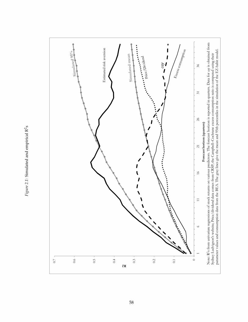
Figu

re2.

1:Si

mul

ated

and

empi

rica

lR2 s

0

0.1

0.2

0.3

0.4

0.5

0.6

0.7

16

1116

2126

3136

R2

Forecast horizon (quarters)

cay

Estimated risk aversion

Note: R2s from univariateregressions of stock returns on various predictors. The forecast horizon is reported in quarters. Data for cayis obtained from

Sydney Ludvigson's website; Price/dividend data comes from CRSP; the Campbell–Cochrane excess consumption ratio is computed using their

parameter values and consumption data from the BEA. The gray lines give the mean and 95th percentiles in the simulation of the EZ-habit model.

58

consumption ratio) over 228-quarter spans in the benchmark simulation of the single-

shock model (the same length as the empirical sample). The upper gray line gives the 95th

percentile of the simulations. As in the data, the simulated R2s rise as the horizon length-

ens. The model compares favorably with the price-dividend and excess-consumption ra-

tios, with the simulated mean tracking the empirical values closely (the median follows

almost the same path). The empirical R2s for cay are at or below the 95th percentile in the

simulations. The only variable that the simulations cannot match is estimated risk aver-

sion, but raising the volatility of risk aversion in the calibration would solve this problem.

The R2s generated here are substantially higher than those obtained in production

models such as Campanale, Castro, and Clementi’s (2010) model of time-varying first-

order risk aversion and Guvenen (2009) and De Graeve et al.’s (2010) studies of limited

participation. The population R2s are also essentially identical to those found by Wachter

(2010) and Gourio (2010) in endowment-economy and production-based models, respec-

tively, with time-varying disaster risk.

The top panel of table 2.3 reports the percentage of simulated samples in which the

simulated R2 is as high as we observe in the data for cay and the price-dividend ratio

(results for excess consumption are similar to the price-dividend ratio), and where a high

price-dividend ratio forecasts low returns. The table reports values for horizons of one

quarter and one through five years. The EZ-CRRA model matches empirical R2s for cay

less than 5 percent of the time at horizons shorter than 16 quarters, but can match the R2s

for the price-dividend ratio 15 to 25 percent of the time. The habit model substantially

raises the likelihood of the simulations of matching the data, by a factor of three or more

at every horizon, and it never matches less than 5 percent of the time except for cay at the

one-quarter horizon.

As an alternative to the R2, I also consider the test statistic suggested by Kiefer, Vogel-

sang, and Bunzel (KVB, 2000) based on Newey–West standard errors with the lag window

equal to the sample size. At various horizons, I calculate the t-statistic on the coefficient

in a regression of stock returns on the price-dividend ratio in the simulated samples. The

bottom panel of table 2.3 repeats the analysis from the top half, but with the KVB test

statistics. In every case, the habit model matches the empirical t-statistics at least five per-

59

Table 2.3: Proportion of simulated samples that match empirical statistics

Forecasting R2

Model:

Predictor: cay P/D cay P/D

Horizon 1 0.00 0.14 0.05 0.52

(quarters) 4 0.01 0.13 0.11 0.52

8 0.01 0.13 0.12 0.51

12 0.02 0.16 0.17 0.56

16 0.04 0.20 0.26 0.62

20 0.10 0.25 0.45 0.69

KVB t-statistics

Model:

Predictor: cay P/D cay P/D

Horizon 1 0.10 0.05 0.38 0.22

(quarters) 4 0.04 0.11 0.17 0.35

8 0.02 0.11 0.08 0.35

12 0.03 0.15 0.12 0.39

16 0.06 0.14 0.22 0.38

20 0.06 0.20 0.19 0.47Note: The top panel reports, for each predictor, the proportion of simulated 228-

quarter samples in which the R2 in a return-forecasting regression is at least as large as

observed in the data and where the predictive relationship has the correct sign. The

bottom panel reports the proportion of simulated samples that generate Kiefer-

Vogelsang-Bunzel t-statistics for each variable that are as large as in the data and have

the same sign. The EZ-habit model is the benchmark (single-shock) model. cay is the

consumption/wealth ratio from Lettau and Ludvigson (2001). P/D is the

price/dividend ratio from CRSP. All simulated regressions use as the predictor the

wealth/consumption ratio (equivalently, the price/dividend ratio on a claim to

aggregate consumption) and the dependent variable is the excess return on a

consumption claim. The regressions are run at horizons listed in the left-hand column.

Bold numbers are less than 0.05, bold italics less than 0.01.

EZ-CRRA

EZ-CRRA

EZ-habit

EZ-habit

60

cent of the time. The EZ-CRRA model again has trouble matching the results for cay, and

only replicates the statistics for the price-dividend ratio in 5 to 20 percent of the samples,

compared to 20 to 50 percent of the samples for the habit model.

2.3.2.2 Other return predictors

Table 2.4 reports the simulated correlation between five-year excess returns on the ag-

gregate wealth portfolio and a variety of return predictors. The first row gives the cor-

relation for actual risk aversion, which we would expect would be highest of all of the

variables. The second row shows that the predictive power of the price-dividend ratio is

nearly as high as that of αt in the benchmark model, but somewhat lower in the dual-shock

calibration (though still not as much lower as in the data).

Fama and Schwert (1977) and Campbell (1987) find that short term interest rates nega-

tively predict future stock returns.27 In table 2.4, I do not replicate the result that the real

interest rate negatively forecasts returns, but the risk-free rate minus its 4-quarter moving

average (denoted RREL as in Campbell, 1987), does weakly negatively forecast returns. Ta-

ble 2.4 shows that the correlation of the five-year excess stock return with the real risk-free

rate and RREL is substantially negative and nearly as large as that of α. In the model, two

effects cause interest rates to forecast stock returns. First, positive technology shocks raise

interest rates and lower risk aversion. Second, even if risk aversion were driven by shocks

unrelated to technology, interest rates might still forecast stock returns since a decline in

risk aversion lowers the precautionary saving effect, raising interest rates. Intuitively, there

is a flight-to-quality effect in interest rates, linking them to expected stock returns.

Table 2.4 reports the mean and standard deviation of the real term spread for the EZ-

habit model. For the sake of simplicity, I follow the literature in modeling long-term debt

as an asset that has a constant probability of paying its principal of one unit of the con-

sumption good and retiring.28 If the bond does not retire and pay out, the holder retains

27 Campbell (1991) subtracts the 12-month moving average of the nominal risk-free rate from itself as a wayto detrend the short term interest rate, since the nominal rate may be nonstationary if there are changes intrend inflation. Detrending in that way should be unnecessary in the model since interest rates are stationary,but I still check this variable.

28 See, e.g. Rudebusch and Swanson (2008) and Miao and Wang (2010).

61

Table 2.4: Various return predictors

Data EZ-CRRA EZ-habit Dual-shock

Five-year excess stock return correlations:

αt 0.69 0.05 0.31 0.27

Real interest rate 0.09 -0.05 -0.30 -0.23

RREL -0.09 -0.03 -0.22 -0.17

Term spread 0.20 0.05 0.29 0.10

P/D -0.39 -0.05 -0.30 -0.23

Term spread summary statistics:

Mean 1.43 -0.14 -0.23 -0.26

Std. dev. 1.17 0.11 0.07 0.14

Note: The bottom two rows are the mean and standard deviation of the spread between the yield on a ten-

year equivalent bond and a one-quarter riskless bond (measured in the data using nominal Treasuries).

The remaining rows give population correlations between various variables and five-year stock retuns. For

the simulations, population values are reported. RREL is the gap between the risk-free rate and its four-

quarter moving average; P/D is the price/dividend ratio. In the simulations, P/D is measured as the

wealth/consumption ratio. ἃ is the value of risk aversion in the model, and estimated in the data as in

section 4.

62

the bond for another period. I assume that the quarterly probability of payout is 1-0.91/4

so that the expected maturity of the bond is ten years. The term spread is the yield to ma-

turity on this bond minus the one-quarter riskless yield. The term spread in the model is

on average negative, whereas the nominal Treasury yield curve is almost always upward-

sloping in the data. The reason we have a negative term spread in the model is that in

good times the marginal product of capital, and hence the risk-free rate, is above average.

So in good times, short-term bonds have low prices, and hence they are a hedge and have

a negative risk premium.

Fama and French (1989) show that the term spread forecasts stock returns. Interest-

ingly, table 2.4 shows that even though the term spread is negative on average in the model,

it still positively predicts future stock returns as in the data. This essentially comes through

an expectations-hypothesis effect. In periods when the risk premium is low, the risk-free

rate is high and expected to fall. To the extent that long-term yields are just averages of ex-

pected future short yields, long yields will rise less than short yields. So in periods when

risk aversion is low, the term spread falls, and the term spread thus positively predicts

stock returns.

In the model, the equity premium is a nearly a constant multiple of αt.29 The variables

that forecast returns in table 2.4 are all correlated with αt, but imperfectly. For example,

the price-dividend ratio also depends on expected consumption growth and interest rates.

The fourth column of table 2.4 shows that the dual-shock model can qualitatively, if not

quantitatively, match the empirical result in column 1 that estimated risk aversion is a

more powerful forecaster of excess stock returns than any of the other variables, since it is

uncontaminated by factors like expected consumption growth.

2.3.2.3 Consumption growth predictability

The aggregate price-dividend and wealth-consumption ratios may be driven by either

movements in expected dividend (consumption) growth or movements in discount rates.

For the aggregate stock market, Campbell and Shiller (1988) and Cochrane (2008) find that

29 This result is exact in the log-linear approximation.

63

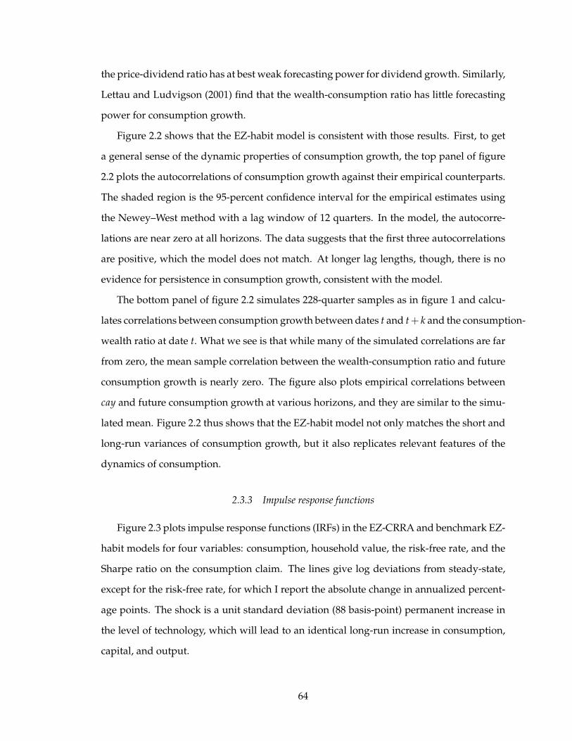
the price-dividend ratio has at best weak forecasting power for dividend growth. Similarly,

Lettau and Ludvigson (2001) find that the wealth-consumption ratio has little forecasting

power for consumption growth.

Figure 2.2 shows that the EZ-habit model is consistent with those results. First, to get

a general sense of the dynamic properties of consumption growth, the top panel of figure

2.2 plots the autocorrelations of consumption growth against their empirical counterparts.

The shaded region is the 95-percent confidence interval for the empirical estimates using

the Newey–West method with a lag window of 12 quarters. In the model, the autocorre-

lations are near zero at all horizons. The data suggests that the first three autocorrelations

are positive, which the model does not match. At longer lag lengths, though, there is no

evidence for persistence in consumption growth, consistent with the model.

The bottom panel of figure 2.2 simulates 228-quarter samples as in figure 1 and calcu-

lates correlations between consumption growth between dates t and t+ k and the consumption-

wealth ratio at date t. What we see is that while many of the simulated correlations are far

from zero, the mean sample correlation between the wealth-consumption ratio and future

consumption growth is nearly zero. The figure also plots empirical correlations between

cay and future consumption growth at various horizons, and they are similar to the simu-

lated mean. Figure 2.2 thus shows that the EZ-habit model not only matches the short and

long-run variances of consumption growth, but it also replicates relevant features of the

dynamics of consumption.

2.3.3 Impulse response functions

Figure 2.3 plots impulse response functions (IRFs) in the EZ-CRRA and benchmark EZ-

habit models for four variables: consumption, household value, the risk-free rate, and the

Sharpe ratio on the consumption claim. The lines give log deviations from steady-state,

except for the risk-free rate, for which I report the absolute change in annualized percent-

age points. The shock is a unit standard deviation (88 basis-point) permanent increase in

the level of technology, which will lead to an identical long-run increase in consumption,

capital, and output.

64

Figure 2.2: Consumption predictability

Note: The top panel reports the empirical autocorrelation function for consumption. The gray shaded region is the 95%

confidence interval using Newey–West standard errors with a lag window of 12 quarters. The bottom panel reports the

correlation of consumption growth between periods t and t+x with the wealth-consumption ratio (cay ) at date t, where x is

reported in quarters on the horizontal axis. The solid lines give the mean and 5th and 95th percentiles of the same correlation

in simulated 228-quarter samples.

-0.8

-0.6

-0.4

-0.2

0

0.2

0.4

0.6

1 6 11 16 21 26 31 36

Forecast horizon (quarters)

Correlation of long-horizon consumption growth with W/C

Empirical estimate

Simulated mean

Simulated 95%

Simulated 5%

-0.4

-0.2

0

0.2

0.4

0.6

1 6 11 16 21 26 31 36

Quarters

Autocorrelation of consumption growth

Empirical estimate

Empirical 95% confidence interval

Model-implied values

65

Figu

re2.

3:Im

puls

ere

spon

sefu

ncti

ons

Note: Im

pulse responses for the EZ-C

RRA and E

Z-hab

its models. The shock is a positive unit-standard-deviation increase in technology. The dotted

lines are for EZ-

CRRA, solid

are for EZ-hab

it. All functions are reported

as fractions of the variables' m

eans except for the risk-free rate, for which the response is in annualized

percentage points. Value is lifetim

e utility; the Sharpe ratio is for an

asset that pays aggregate co

nsumption as its dividen

d.

0

0.001

0.002

0.003

0.004

0.005

0.006

0.007

0.008

16

11

16

21

26

31

36

41

Consumption

-0.14

-0.12

-0.1

-0.08

-0.06

-0.04

-0.020

16

11

16

21

26

31

36

41

Sharpe ratio

0

0.002

0.004

0.006

0.008

0.01

0.012

16

11

16

21

26

31

36

41

Value

EZ-C

RRA

EZ-hab

it

0

0.01

0.02

0.03

0.04

0.05

0.06

0.07

16

11

16

21

26

31

36

41

Risk-free rate (levels)

66

The top-left panel shows the response of household value. For the EZ-CRRA model,

value immediately jumps to a point just below its new steady state, and then slowly rises

as households accumulate capital. For the EZ-habit model, though, value actually over-

shoots its new steady state. The reason is that the positive shock to productivity drives

risk aversion down. When households are less risk-averse, they place a higher value on

their future consumption stream because they penalize uncertainty less strongly. This ef-

fect helps increase the volatility of the SDF (equation 2.6), raising the Hansen–Jagannathan

bound. The top-right panel shows that on the impact of a shock, the Sharpe ratio in the

EZ-habit model falls by 12.5 percent (as a fraction of its mean), and then gradually rises

again, with a half-life of 12 quarters.

The bottom-left panel shows the dynamics of the risk-free rate. The initial response

is essentially identical for the two models. The reason for this is that the risk premium

on an unlevered claim on capital is very small in the model, so the return on capital is

roughly equal to the risk-free rate. Since the size of the capital stock is essentially fixed in

the short-run, an increase in productivity directly increases the return on capital and hence

the risk-free rate.

The final panel of figure 2.3 shows the response of consumption in the two models.

The EZ-habit model shows a larger initial response of consumption, with lower expected

consumption growth going forward. To see why this is, we can write consumption growth

in equilibrium as

Et∆ct+1 = c + ρ−1r f ,t+1 + αt × vol (2.15)

where r f ,t+1 is the risk-free interest rate between dates t and t+ 1, vol represents a measure

of the total volatility in the model, and c is a constant. αt× vol represents the precautionary

saving effect and is a function of the current level of risk aversion and the variances of

the shocks in the model. The standard interpretation in an endowment economy is that

conditional on consumption growth, a strong precautionary saving motive leads to a low

risk-free rate. In a production setting, though, it is the risk-free rate that is held roughly

fixed since it is tied to the marginal product of capital, which is hard to change quickly

through investment. Conditional on the risk-free rate, then, a small precautionary saving

67

motive leads to lower expected consumption growth (more consumption today, saving less

for tomorrow). In the EZ-habit model, a positive technology shock lowers risk aversion,

and hence consumption rises more than in the canonical EZ case. This effect also serves to

increase the volatility of the SDF, just as the higher response of value does.

Given the results in figure 2.3, it is straightforward to see what would happen in this

economy if there were a pure shock to the coefficient of relative risk aversion. Since the

risk-free rate is tied to the marginal product of capital, it would not move on the impact

of a shock. The only effect on real variables of a pure decline in risk aversion then is that

households would want a smaller buffer stock of savings, so they would raise consump-

tion and lower investment: shocks to risk aversion look like simple demand shocks.

2.3.4 Estimating the EIS from interest rate regressions

The value of the elasticity of intertemporal substitution is controversial. Regressions

based on aggregate consumption and asset returns often find a very small EIS (Hall, 1988;

Campbell and Mankiw, 1989). Campbell (2003) reviews the literature and estimates the EIS

using a variety of specifications and data from a broad range of countries, finding values

generally less than 0.5 and often less than 0.2.30 This result is in conflict with the calibration

used here and in other recent production-based asset pricing studies (Kaltenbrunner and

Lochstoer, 2010; Gourio, 2010), which assume that the EIS is greater than 1. The question is

whether the EZ-habit model generates small EIS estimates in regressions similar to those

estimated in Campbell (2003).

The standard aggregate EIS regressions start from a model in which the risk-free rate

takes the form

r f ,t+1 = b0 + ρEt∆ct+1 (2.16)

where r f ,t+1 is the riskless interest rate between periods t and t + 1. b0 is a parameter

depending on the discount rate and underlying volatility in the model (which are taken

30 Vissing-Jorgenson (2002) finds an EIS less than unity in micro data. On the other hand, Vissing-Jorgensonand Attanasio (2003) and Gruber (2006) obtain larger estimates using micro data, both above unity. Gruber(2006) is particularly well-identified, using variation in the capital income tax rate as the source of exogenousdifferences in the after-tax interest rate earned by households.

68

to be constant). This relationship is straightforward to derive in an endowment economy

with homoskedastic consumption growth and where households have a constant EIS and

coefficient of relative risk aversion. It is also obtained in a log-linearization of the standard

RBC model with homoskedastic technology shocks.

In principle, the EIS can be estimated from a regression of interest rates on consumption

growth or vice versa. However, since the reduced-form relationship between consumption

growth and interest rates is nearly zero in the EZ-habit model, in some of the simulations

regressing Et∆ct+1 on r f ,t+1 produces explosive estimates for ρ−1 (since we have to invert

the coefficient estimate). Moreover, consumption in the EZ-habit model nearly follows a

random walk, so it is essentially unpredictable and there are serious weak-instruments

problems in an IV regression of interest rates on consumption growth. I therefore focus on

the regression of consumption growth on interest rates,

Et∆ct+1 = b′0 + ρ−1r f ,t+1 (2.17)

In the simulations of the model in section 2.3, we have the ability to directly measure

Et∆ct+1. The first row of table 2.5 reports the population estimate of ρ−1 in regression (2.17)

under the EZ-CRRA and EZ-habit models. In the EZ-CRRA case, the regression identifies

ρ−1 exactly. On the other hand, the estimate of ρ−1 is biased substantially downwards in

the EZ-habit specifications.

The bias comes from the fact that the time-varying precautionary saving effect (equa-

tion 2.15) is omitted from the regression. Since precautionary saving is correlated with both

expected consumption growth and interest rates, omitting it biases the simple IS-curve re-

gression usually used to identify the EIS. An alternative way to see the source of the bias

is to go back to the IRFs in figure 2.3. In both models the risk-free rate rises by the same

amount following a shock. In the EZ-habit specification, though, because of the decline

in precautionary saving, expected consumption growth is lower following a shock than in

the EZ-CRRA case. That means that the estimate of ρ−1 will fall.31

31 In Bansal and Yaron (2004), time-variation in the volatility of shocks in principle causes EIS regressions tobe biased. However, Beeler and Campbell (2010) show that their calibration generates almost no actual bias—the median sample EIS estimates are well above 1. This paper thus represents an improvement in being able

69

Table 2.5: Regressions estimating the elasticity of intertemporal substitution

Model: Data EZ-CRRA EZ-habit Dual-shock

1 Population, infeasible (Et[∆ct+1]) N/A 1.50 0.64 0.78

2 Population N/A 1.50 0.56 0.71

3 Small sample 0.14 1.16 0.03 0.35

4 [2.5%, 97.5%] N/A [0.03, 1.79] [-1.98, 1.02] [-1.32, 1.34]

5 Population, RRA control N/A N/A 1.50 1.50

6 Small sample, RRA control 0.18 N/A 0.07 0.94

7 [2.5%, 97.5%] N/A N/A [-3.08, 3.11] [-1.07, 2.78]

Note: Values reported are the coefficient from regressions of consumption growth or expected consumption

growth on the risk-free rate. The dependent variable in row 1 is expected consumption growth (computed

numerically in the simulations); all other rows use actual consumption growth. The small-sample regressions are

based on 228 quarters of data, and median coefficient estimates are reported; 2.5 and 97.5 percentiles are

reported in brackets. The RRA control is actual risk aversion in the simulations and estimated risk aversion

(section 4) in the empirical regressions.

70

The regression in the first row of table 2.5 is in some sense ideal, but it is not the re-

gression that we are actually able to run in the data since Et∆ct+1 is unobservable.32 Rows

2 through 4 report results for estimates of ρ−1 from regressions of actual consumption

growth, ∆ct+1, on the risk-free rate, r f ,t+1. Row 2 gives the population estimates, while

rows 3 and 4 give the median and 95-percent range of the estimates from 228-quarter sim-

ulations. With constant relative risk aversion, the population regression in row 2 estimates

the EIS exactly. The median estimate from the small-sample regressions in row 3 is 1.16.

The 95-percent range is wide, and it only just barely contains the estimate from the data.

So it is in principle possible for the EZ-CRRA model to generate an estimate of the EIS as

small as what we observe in the data, but the probability is small (less than 10 percent).

In the EZ-habit models, the bias is far larger. The population estimate in the single-

shock case is 0.56, and the median sample estimate is 0.03. For the dual shock model,

the estimates are only slightly better—0.71 in population and a median of 0.35 in small

samples. The reason for this slight improvement is that the temporary shocks have little

effect on risk aversion, so they induce variation in consumption and the risk-free rate that is

closer to the usual EZ-CRRA case. The upper end of the 95 percent range for the simulated

estimates is well below the true value of the EIS.

The first four rows of table 2.5 show that in general, regressions of interest rates on

expected consumption growth are not a very good way to estimate the EIS, and in the EZ-

habit model they are biased and inconsistent. It is worth noting, though, that if we could

observe αt, we could completely eliminate the bias in the EIS regressions. Empirically, this

suggests that regressions designed to estimate the EIS could be improved by including a

control for risk aversion, such as the price-dividend ratio on the stock market. The final

three rows of table 2.5 try to estimate the EIS including a control for risk aversion. In the

data, I use a measure of risk aversion derived from the EZ-habit model below in section

to generate a substantial bias in aggregate regressions without large movements in the conditional volatilityof consumption.

32 In principle, the real risk-free rate, r f ,t+1, is also unobservable in the data. As above, I form r f ,t+1 as thedifference between the nominal 3-month interest rate and a forecast of inflation based on lagged inflation andnominal interest rates. Errors in the estimate of the true real-risk-free rate would bias the estimate of ρ−1

towards zero. Instrumental-variables methods can theoretically eliminate this bias.

71

2.4, denoted αt. The empirical estimate of the EIS is essentially unchanged from when

αt is not included. In population, when αt is included in the simulated regressions, the

EIS is estimated exactly. In small-sample regressions, though, the estimate of the EIS in

the model is still biased downward. In the single-shock model, the median estimate is

0.07. and in the dual-shock model 0.94. Row 7 shows, though, that the 2.5 percentile of

the small-sample estimates is -3.08 in the dual shock model, while the 97.5 percentile is

3.11. So even though the median estimate in the dual-shock model is not enormously

biased, the empirical value of 0.18 is well within the simulated range. In the end, while

controlling for risk aversion should, in principle, allow us to estimate the EIS consistently,

in small samples the regressions still do not seem to provide useful estimates because of

weak-identification problems.

As an alternative to these regressions, the EIS could be consistently estimated if we

had an instrument for the risk-free rate that was uncorrelated with risk aversion. Standard

aggregate instruments like lagged interest rates and consumption growth (e.g. Campbell,

2003) will certainly not be valid instruments under the EZ-habit model since the precau-

tionary saving effect is persistent. Household-level instruments would work better if my

model is correct in treating risk aversion as being driven by aggregate factors.33 The EZ-

habit model thus has the ability to explain the divergence between micro and macro esti-

mates of the EIS if the micro instruments are valid and the macro instruments invalid.

2.4 Empirical return forecasting

This section shows how the model suggests we can directly estimate the coefficient of

relative risk aversion in the data, and then demonstrates that the estimate is a powerful

predictor of stock returns. Second, I present novel evidence that technology growth fore-

casts stock returns, just as it does in the production model. The results differentiate the EZ-

habit paper from models with time-varying disaster risk. Gourio (2010) predicts that when

33 Gruber (2005) discusses precisely these issues and tries to resolve them by using household-specific vari-ation in tax rates as an instrument for consumption growth. Dynan (1993) explicitly controls for the precau-tionary savings effect at the household level by predicting the conditional volatility of consumption, but shedoes not deal with the possibility that risk aversion varies over time.

72

there are changes in the probability of a large disaster occurring, price-dividend ratios will

forecast returns, which is also true in the EZ-habit model. The EZ-habit model also pre-

dicts, though, that technology and estimated risk aversion will forecast stock returns, and

that estimated risk aversion will be the single most powerful forecaster of returns, which

would not be true in the time-varying disaster model or models based on other forms of

time-varying volatility (e.g. Bansal and Yaron, 2004, Bloom, 2009, or Fernandez-Villaverde

et al., 2011).

2.4.1 Estimating risk aversion

If risk aversion follows the AR(1) process given in (2.5), then we can measure current

risk aversion if we simply observe the history of aggregate value, vAt . For a given value

of the EIS and observed data on wealth and consumption, it is possible to calculate vAt by

rearranging equation (2.7)

vAt =

11− ρ

wAt −

ρ

1− ρcA

t +1

1− ρlog (1− exp (−β)) (2.18)

If we can measure household wealth and consumption, then we can measure value. We

then simply plug the estimates of vAt into equation (2.5) to obtain estimates of αt.

Lettau and Ludvigson (2001) study a cointegrating relationship between consumption

and aggregate wealth. Their method is valid in my model since consumption and wealth

are cointegrated under balanced growth. While their analysis was designed to estimate

the consumption-wealth ratio, it also delivers, as a byproduct, a measure of aggregate

wealth (since we can always add consumption to the wealth-consumption ratio to obtain

wealth). The estimate of wealth derived using their method is a combination of asset

wealth data obtained from the flow of funds accounts plus an estimate of human wealth.

They treat labor income as the dividend from the stock of human wealth. Assuming the

price-dividend ratio for human wealth is stationary, we can use labor income as a proxy

for human wealth. Denoting asset wealth as at and labor income as yt, the appendix shows

73

that we then have a cointegrating relationship,

ct = ζωat + ζ (1−ω) yt + ξ ′t (2.19)

where ζ and ω are parameters and ξ ′t is a stationary error term. Lettau and Ludvigson

(2001) refer to the residual ξ ′t as cay. This variable essentially represents an estimate of the

consumption-wealth ratio. Since I want to estimate wealth, I define

ayt ≡ ωat + (1−ω) yt (2.20)

which, under the assumptions above, will be a statistically unbiased estimate of total

wealth, but will include error due to the fact that we do not assume we directly measure

human wealth.34

With our measure of wealth ayt, we estimate vAt as

vAt =

11− ρ

ayt −ρ

1− ρct (2.21)

where we ignore constants, and a circumflex indicates an estimated variable. Note that

since the parameters of the cointegrating relationship for ct, at, and yt are estimated super-

consistently we do not have to modify any standard errors in the subsequent analysis to

take into account the fact that ayt is a generated regressor (which is why it does not receive

a circumflex). That said, to the extent that there is measurement error in the consumption

or wealth data, vAt will inherit that same error. When we use vA

t to forecast market returns,

this measurement error should only weaken the results. For measurement error to gener-

ate a spurious predictive relationship, it would have to be correlated with other predictors

of returns.35

34 In simulations with variable labor supply, The price/dividend ratio on human wealth does vary overtime, but the variation is relatively small: risk aversion calculated using the method here (assuming a constantprice-dividend ratio on human wealth) is over 95 percent correlated with actual risk aversion.

35 One obvious source of measurement error is that human capital is not a perfect estimator of the valueof human wealth. Suppose risk aversion rises above average and lowers the price-dividend ratio on humanwealth below average. Labor income will then be overestimating human wealth (compared to its average).High levels of wealth drive out measure of αt downward, so this measurement error should bias the resultsagainst correctly forecasting returns (high risk aversion in the data leads to low risk aversion in our estimates).

74

This definition of vAt is similar to Lettau and Ludvigson’s cayt, except they have equal

weights on ct and ayt, whereas equation (2.21) uses a combination where the weights de-

pend on the EIS. Also, cayt is stationary by construction, whereas vAt is growing over time

(it is cointegrated with consumption and wealth).

In equation (2.21) a high EIS (low ρ) raises the weight on consumption relative to asset

wealth. If the EIS is less than 1 (ρ > 1), the weight on wealth, ayt, is actually negative, and

the weight on consumption greater than 1. Bansal and Yaron (2004) and Kaltenbrunner

and Lochstoer (2010) both find that an EIS of 1.5 allows their models to fit asset pricing

facts, so I use the same value. This value is also consistent with the micro evidence of

Vissing-Jorgensen and Attanasio (2003). The results reported below are broadly similar as

long as the EIS is greater than 1.1 (at that level and below, vAt becomes very volatile). The

appendix reports a sensitivity analysis for various values of the EIS.

Figure 2.4 plots vAt both in its raw levels and with a linear trend taken out. As we would

expect, vAt follows a strong upward trend. There seem to be both low and high frequency

components to detrended vAt . In particular, there are long-run swings with peaks in the

early 1970’s and 2000’s and a trough around 1994, generally consistent with movements in

the aggregate price-dividend ratio and variation in average output growth.36 At the same

time, there are business-cycle frequency movements, e.g. the troughs in 1973, 2001, and

2008.

I construct an estimate of αt, αt, using the update process for risk aversion, equation

(2.5), and the data on vAt . In particular, we have

αt+1 = φαt + (1− φ) α + λ(

∆vAt+1 − Et∆vA

t+1

)(2.22)

As above, I assume that φ = 0.96. Et∆vAt+1 is estimated simply as the sample average of

∆vAt .37

In the simulations not reported here, though, this effect seems to be small.

36 Note, though, that linear detrending will tend to make the series look as if it is mean-reverting even if itfollows a random walk. The linear trend is only used to make the graph legible; none of the results involve it.

37 In principle, it is possible to forecast ∆vAt+1, but the amount of predictability in ∆vA

t+1 is sufficiently smallthat the results are nearly identical to assuming that vA

t+1 simply follows a random walk.

75

Tabl

e2.

6:V

alue

,raw

and

linea

rly

detr

ende

d

-0.2

-0.1

5

-0.1

-0.0

5

00.0

5

0.1

0.1

5

0.2

0.2

5

9.5

9.7

9.9

10.1

10.3

10.5

10.7

10.9

11.1

11.3

11.5

1952

1957

1962

1967

1972

1977

1982

1987

1992

1997

2002

2007

Note

: H

ouse

hold

value (lifet

ime utility

)is m

easu

red u

sing

dat

a on w

ealth and consu

mption fro

m S

ydney

Ludvig

son's w

ebsite

. The

thin

lin

e is the

abso

lute

level o

f value (lef

t-han

d a

xis); t

he

thick lin

e is v

alue linea

rly det

rended

. Both

var

iables ar

e m

easu

red in logs

. Gre

y bar

s ar

e N

BER-d

ated

rec

essions.

Log house

hold

value

(lifet

imeutilit

y)Log

house

hold

value,

linea

rly det

rended

76

The parameter λ governs the volatility of αt, but it has only a multiplicative effect on

αt. That is, two estimates of αt will be perfectly correlated with each other, regardless of

what values are chosen for λ. The same argument applies for α. As long as we are simply

trying to forecast stock returns using a linear regression, we can ignore any additive or

multiplicative shifts in αt. Therefore, I set α = 0 and choose λ so that αt has unit variance,

normalizations that will have no effect on the regression-based measures of forecasting

power (and I choose a negative value of λ to match the habit-formation motivation of the

model). In the first period of the sample I assume α = α.

An important feature of this method of forecasting is that it is based only on the pref-

erence specification. None of the assumptions we made about the production side of the

economy are required for this method to be valid. We simply take advantage of the rela-

tionship between household value and changes in risk aversion and the relationship under

Epstein–Zin preferences between household value and wealth.

2.4.2 Forecasting market returns

The next question is to what extent the model-implied variation in expected returns is

related to actual returns. Figure 2.5 plots αt and 5-year excess returns on the stock market

(the value-weighted excess return from Kenneth French). The strong correlation between

the two series (0.68) is immediately apparent. There are both high and low-frequency

movements in αt associated with changes in growth in value. In the periods when value is

growing quickly, e.g. the late 1990’s, risk aversion falls. At the same time, there are higher-

frequency movements, such as the temporary increases in estimated risk aversion around

the recessions in 1991 and 2001.

Figure 2.1 plots R2s from regressions of future stock returns on αt, cayt, the price-

dividend ratio (P/D), and the excess consumption ratio from Campbell and Cochrane

(1999). Each line gives the R2 from a univariate regression. The x-axis gives the hori-

zon for the return in quarters. The nth point is the R2 from a regression of ∑nj=1 rt+j on

the predictor at time t. The regressions are all run on quarterly data from 1952 to 1999 (to

The appendix shows that the results are robust to different choices for φ.

77

Figu

re2.

4:Es

tim

ated

risk

aver

sion

and

5-ye

arex

cess

stoc

kre

turn

s

-2.5

-1.5

-0.5

0.5

1.5

2.5

3.5

4.5

5.5

6.5

-4-3-2-101234

19

52

19

57

19

62

19

67

19

72

19

77

19

82

19

87

19

92

19

97

20

02

20

07

Excess returns

Estimated risk aversion (normalized)

5-y

ear

exce

ssst

ock

ret

urn

sE

stim

ated

risk

av

ersi

on

No

te:

Exc

ess

sto

ckre

turn

s ar

e fo

r th

e C

RS

P v

alu

e-w

eigh

ted

ind

ex m

inu

s th

e ri

sk-f

ree

rate

, fr

om

Ken

Fre

nch

's w

ebsi

te. R

etu

rns

are

forw

ard

-lo

ok

ing

fiv

e-ye

ar a

ver

ages

. Ris

k a

ver

sio

n i

s es

tim

ated

fro

m d

ata

on

agg

rega

te w

ealt

h a

nd

co

nsu

mp

tio

n a

nd

is

no

rmal

ized

to

hav

e ze

ro m

ean

an

d u

nit

var

ian

ce.

78

ensure we have data for the 40-quarter regression). Each regression uses the same sample

for the predictors.

At every horizon, α is dominant. At the five-year horizon, the R2 for estimated risk

aversion peaks at more than twice that of the other variables. The R2s are impressively

high for just a single variable: at the 5-year horizon, α explains 50 percent of the post-

war variation in stock returns. Furthermore, in horse-race regressions (reported in the

appendix), α dominates cay at all horizons.

An important consideration in long-horizon forecasting regressions is that the residuals

are highly persistent. Kiefer, Vogelsang and Bunzel (2000) and Kiefer and Vogelsang (2005)

show that by using Newey–West standard errors with a very long lag-window, we can

obtain test statistics with better size properties than techniques that use a fixed (and usually

short) lag window. I choose a lag window equal to half the sample size and use the critical

values reported in Kiefer and Vogelsang (2005).38 For cay, every regression except for

those with horizons greater than 30 quarters is significant at the 5 percent level. For α, the

largest p-value is 0.0008. The price-dividend ratio is significant at the 5 percent level for

forecasts of 14 quarters or longer. In other words, these regressions all imply that we have

substantial ability to forecast stock returns in the post-war period, and α is the strongest of

the predictors. Out-of-sample tests with both asymptotic and bootstrapped critical values

give similar results (appendix D.3). Appendix D examines the sensitivity of the results in

this section to the various parameters we had to calibrate (e.g. the EIS and the persistence

of habits). The basic results hold across a broad range of parameter sets.

2.4.3 Forecasts from estimates of technology

The method of estimating the level of risk aversion studied above does not rely on

any assumptions about the structure of production in the economy, being derived purely

from the preference specification. However, in the production model, changes in value are

38 Kiefer and Vogelsang (2002) note that there is a size-power tradeoff. When the lag window is increased,the size of the test statistics gets closer to their nominal size, but there is a loss of power. I choose a lag windowof half the sample to balance these considerations. The results are basically identical when using a lag windowequal to the sample size as in Kiefer, Vogelsang, and Bunzel (2000), though the price-earnings is significant inmore of the regressions.

79

closely related to changes in productivity. If we can measure innovations to technology,

then risk aversion should follow an AR(1) process where the innovations are equal to the

shocks to the stochastic trend in technology.

There is a large literature that tries to estimate aggregate technology shocks. I consider

two methods here. The first builds off of Solow (1957) and uses restrictions from a constant-

returns production function:

at = yt − γkt − (1− γ) lt (2.23)

at measures technology if the economy has a Cobb–Douglas production function, with

l denoting log labor supply. I also consider a simpler metric, labor productivity, lpt =

yt − lt. Labor productivity does not take into account the effects of capital accumulation

and simply models technology as the average product of labor. Capital can be difficult

to measure, whereas the number of hours supplied in the economy is a fairly concrete

quantity (though the quality of those hours is difficult to account for).39

To extract the stochastic trend from the two productivity series, I estimate univariate

ARMA models for each variable. The Bayesian information criterion implies that TFP

growth is best fit with an MA(2), while labor productivity growth should be treated as i.i.d.

εTFPt is defined as the residual in the MA(2), while εLP

t is simply equal to labor productivity

growth. That is, εTFPt and εLP

t are innovations to the Beveridge–Nelson (1981) trends in

productivity.

Section 2.5.1 shows that, at least in the case where log technology follows a random

walk, risk aversion follows an AR(1) process of the form,

αt = (1− θ) αt + θαt−1 + εXt (2.24)

where εX denotes a measure of technology growth. We then have two measures of αt,

39 Furthermore, labor productivity determines the tradeoff that households face between consumption andleisure. If the capital stock rises because foreigners want to invest more in the US, household welfare willincrease even if TFP does not. Similarly, a tax increase that reduced desired saving could lower welfare andlabor productivity, without having any effect on TFP. And welfare is the relevant input in estimating αt.

80

which I denote αTFP, αLP, using εTFPt and εLP

t , respectively.40 The two measures turn out to

be highly correlated (93 percent).

Figure 2.6 plots five-year excess returns against αTFP and αLP The two series are both

clearly highly correlated with future excess returns. The p-values in regressions of quar-

terly excess returns on αTFP and αLP are 0.032 and 0.026, respectively (using Kiefer, Vogel-

sang, and Bunzel, 2000, t-type-statistics to account for autocorrelation). The relationship

between the three series is most clear around the turning points. Productivity growth be-

gins slowing down around 1970, driving risk aversion upwards. Forward-looking stock

returns reach their trough at roughly the same point. Productivity growth rises again start-

ing in the mid-1990’s, which is exactly when stock returns begin falling again.

The two measures of risk aversion in figure 2.6 clearly do not have the explanatory

power of the variables studied above. The wealth and consumption data used above have

a forward-looking component that is not present in instantaneous measures of technology.

On the other hand, my measure of risk aversion is highly correlated with the consumption-

wealth ratio. In almost any model with time-varying discount rates, the consumption-

wealth ratio will forecast stock returns. It is not the case, though, that any model will

predict that measures of technology should forecast stock returns. Figure 2.6 thus provides

evidence in favor of the model presented here over other explanations of time-varying

expected returns.

2.5 Extensions

2.5.1 Log-linearization

This section studies a log-linear version of the production economy from above. I use

the solution to build a better understanding of the basic results reported in the previous

sections. In particular, I derive analytic approximations for the consumption function,

the risk-free rate and the conditional Sharpe ratio for the wealth portfolio. I also derive

40 Note that αTFP includes some forward-looking information since its construction requires the estimationof an MA(2) on the full sample. αLP does not suffer from this flaw. It is true that in both cases we have toestimate mean productivity growth, but shifts in the estimted mean simply correspond to shifts in the meanof αt; they have no effect on its dynamics. In regressions of returns on αt, the constant will thus always absorbshifts in α, so the estimation of the mean of productivity growth is irrelevant for forecasting returns.

81

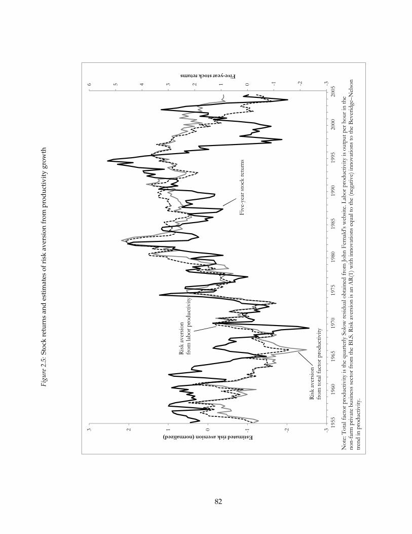
Figu

re2.

5:St

ock

retu

rns

and

esti

mat

esof

risk

aver

sion

from

prod

ucti

vity

grow

th

-3-2-10123456

-3-2-10123

1955

1960

1965

1970

1975

1980

1985

1990

1995

2000

2005

Five-year stock returns

Estimated risk aversion (normalized)

Five-yearstock returns

Riskaversion

from labor productivity

Risk aversion

from total factor productivity

Note: Totalfactor productivity is the quarterly Solow residual obtained from John Fernald's website. L

abor productivity is output per hourin the

non-farm private business sector from the BLS. R

isk aversion is an AR(1) with innovations equal to the (negative) innovations to

the Beveridge–Nelson

trend in productivity.

82

an essentially affine model of the term structure with a time-varying price of risk. This

result connects the standard production theory in the macro literature to one of the most

commonly used empirical asset-pricing frameworks.

2.5.1.1 Approximation method and solution

I derive a log-linear consumption function as the solution to a model that represents

a log-linearization of the environment derived above with permanent technology shocks

only. Specifically, if the capital accumulation equation, the return on capital, and the return

on the wealth portfolio are log-linearized, then we are able to obtain an exact formula for

the consumption function under EZ-habit utility (with canonical Epstein–Zin and power

utility as special cases). The methods build on Campbell (1994) and Lettau (2003). Un-

like the usual techniques in the macro literature, the solution is not based on certainty-

equivalent or higher-order approximations to expectations.41 Rather, I take advantage of

log-normality to calculate expectations exactly. That feature of the method is critical for

accurately capturing risk premia and precautionary saving effects.

It is straightforward to show that the approximation technique delivers policy func-

tions that are identical to those obtained from perturbation up to the first order (depend-

ing on where the derivatives are taken). The difference is that because I take advantage

of formulas for log-normal expectations, a term involving risk aversion appears in the so-

lution, meaning that the approximation captures the time-varying precautionary saving

effect that is central to driving the difference in the consumption response between the

EZ-habit model and the RBC model with canonical Epstein–Zin preferences.42

The approximation method involves log-linear approximations to three components

of the model: the budget constraint, the return on the wealth portfolio, and the return on

41 The usual technique is the perturbation method of Judd (1999). See Woodford (2003) for a representativeapplication and Rudebusch and Swanson (2009) for extensions to higher order approximations

42 In perturbation, the equilibrium equations are not only approximated with respect to the endogenous andexogenous variables, but also the volatility of the technology shock, σa. The first-order perturbation solutiontherefore does not include any terms involving interactions of state variables with σa. The approximation usedhere includes a term for αtσ

2a . The solutions are otherwise identical.

83

capital,

kt+1 ≈ λ0 + λkkt + λaat + λcct (2.25)

rw,t+1 ≈ Etrw,t+1 + ∆Et+1

∞

∑j=0

θ j∆ct+j+1 − ∆Et+1

∞

∑j=1

θ jrw,t+j+1 (2.26)

rk,t+1 ≈ r0 + rk (kt+1 − at+1) (2.27)

where {λ0, λk, λa, λc, θ, r0, rk} are linearization coefficients that I solve for in the appendix

and lower-case letters denote logs.43

Define ct ≡ ct− at and kt ≡ kt− at. With the the three log-linear approximations (2.25),

(2.26), and (2.27), the appendix shows that we can obtain the following result:

Proposition 2.1. Given the log-linear budget constraint, the log-linear return on the consumption

claim, and the production function, the optimal consumption plan takes the form

ct = ηc0 + ηck kt + ηcaαt (2.28)

and the return on the wealth portfolio can be written as

rw,t+1 = ηw0 + ηwaαt + ρEt∆ct+1 + κrεt+1 (2.29)

where the coefficients {ηc0, ηck, ηca, ηw0, ηwa, κr} are solved for in the appendix. Furthermore, the

log price-dividend ratio of the consumption claim is linear in risk aversion and scaled capital.

The first important implication of this result is that even though risk aversion is time-

varying, both consumption growth and returns on the wealth portfolio are homoskedastic.

We did not assume the existence of a log-linear policy for consumption or homoskedastic

wealth return. Variation in risk aversion induces variation in expected returns on risky

assets, but not in their volatility. This same result is obtained in the numerical solution

above.

43 (2.25) is a log-linearization of the resource constraint, Kt+1 = (1− δ)Kt + A1−γt Kγ

t − Ct; (2.26) is theCampbell–Shiller (1988) approximation for the return on the wealth portfolio; (2.27) is a linearization ofRk,t+1 = γKγ−1

t+1 A1−γt+1 + 1− δ.

84

Remark 2.1. ηck does not depend on the level or volatility of the coefficient of relative risk

aversion (i.e. on α or λ).

The finding that ηck is not affected by the time-variation in the coefficient of relative risk

aversion helps us build intuition as to why the IRF for consumption changes when risk

aversion varies. Consumption responds to a technology shock more strongly in the EZ-

habit model than in the RBC model purely because the coefficient of relative risk aversion

falls in response to positive technology shocks. If the economy experienced a hypothetical

shock to the size of the capital stock holding the coefficient of relative risk aversion fixed,

the behavior of consumption and saving would be identical under EZ-habit and EZ-CRRA

preferences.

2.5.1.2 The risk-free rate and excess returns on the wealth portfolio

Denote the conditional standard deviation of a variable x as σ (x). We have the follow-

ing formulas for the risk-free rate and Sharpe ratio,

Proposition 2.2. In the log-linearized model, the risk-free rate follows

r f ,t+1 = η f 0 + ρE∆ct+1 − η f aαt (2.30)

and the Sharpe ratio of the consumption claim is

Etrw,t+1 − r f ,t+1 +12 σ2 (rw)

σ (rw)= ρσ (∆c) + (αt − ρ) σ (∆v) (2.31)

As usual, expected consumption growth affects the risk-free rate in proportion to the

inverse of the EIS. There is an additional term η f aαt reflecting the time-varying precau-

tionary saving motive. When risk-aversion is high, precautionary saving demand is high,

driving the risk-free rate downwards, all else equal. It is immediately clear that a simple

regression of consumption growth on interest rates will not identify the EIS, 1/ρ, unless

the instruments used for the interest rate are uncorrelated with current risk aversion or

risk aversion is controlled for.

Note also that the Sharpe ratio is strictly increasing in αt. The terms σ (∆c) and σ (∆v)

85

are the standard deviations of growth in household consumption and value, respectively

(both of which are constant in equilibrium). Tallarini (2000) and Lettau (2003) show that

in an RBC model with power utility, an increase in risk aversion need not increase the

Sharpe ratio because consumers can endogenously smooth consumption.44 In this setting,

though, risk aversion unambiguously increases the Sharpe ratio. The reason is that the

preference for consumption smoothing comes from the EIS. An increase in risk aversion

does not cause consumers to smooth consumption endogenously, and so the only effect is

to raise the Sharpe ratio on the wealth portfolio.

An obvious question is what the term σ (∆v) actually is. The appendix derives the

following results,

Proposition 2.3. In equilibrium, the coefficient of relative risk aversion αt follows the process,

αt = φαt−1 + (1− φ) α + σaaεt (2.32)

where σaa depends on the parameters λ, θ, φ, and σa.

The standard deviation of innovations to value is

σ (∆v) =−1 +

√1 + 2 θ

1−θφ σaaσa

θ1−θφ σaa

(2.33)

σ (∆v) is increasing in σa for σa > 0 and σaa < 0.

Result 2.3 first shows that the coefficient of relative risk aversion follows an AR(1) pro-

cess with innovations that are perfectly correlated with technology shocks. This result is a

consequence of household value being a log-linear function of the level of technology, so

that vt+1 − Etvt+1 is a linear function of the technology shock.

Result 2.3 shows that the standard deviation of innovations to household value is con-

stant. Furthermore, in the benchmark case where technology shocks drive risk aversion

down, an increase in their volatility raises the volatility of innovations to value, as we

would expect.

44 Lettau and Uhlig (2004) and Rudebusch and Swanson (2008) obtain similar results for Campbell–Cochranepreferences.

86

In the case where σaa = 0, which corresponds to power utility, we obtain a surprisingly

simple formula:

Remark 2.2. For the RBC model where technology follows a random walk and consumers

have constant relative risk aversion, the Sharpe ratio on a consumption claim is approxi-

mately

SRt ≈ ασa (1− ηck) + (α− ρ) σaηck (2.34)

≈ ασa − ρσaηck (2.35)

This formula is similar to the formula obtained by Bansal and Yaron (2004) for the

Sharpe ratio in the presence of long-run risks in an endowment economy. σa represents

long-run shocks to consumption growth, since consumption eventually catches up to a

technology shock. Of that total response, σa (1− ηck) comes in the first period, with σaηck

in subsequent periods.45 We can thus think of the first component of the Sharpe ratio,

ασa (1− ηck), as Bansal and Yaron’s short-run risk term, and (α− ρ) σaηck as long run risks.

Kaltenbrunner and Lochstoer (2010) also show that production models generate long-run

risk endogenously, but this simple formula for the Sharpe ratio has not been obtained

elsewhere.

The second line shows that we can isolate the ηck term. If the EIS is large (ρ is small) then

the endogenous response of consumption in the model is unimportant and the Sharpe ratio

is determined simply by the volatility of technology shocks and the coefficient of relative

risk aversion.

2.5.2 Affine bond pricing

It turns out that the log-linear solution to the model allows us to connect the standard

macro framework to the bond-pricing literature through the following result:

45 Recall that ηck is the coefficient on scaled capital in the consumption function. A unit increase in the tech-nology shock εt+1 raises consumption by σa; the associated decline in scaled capital of σa lowers consumptionηckσa.

87

Proposition 2.4. The log stochastic discount factor can be expressed as

mt+1 = −r f ,t+1 −12(ω0 + ω1αt)

2 σ2 + (ω0 + ω1αt) εt+1 (2.36)

The SDF takes the tractable essentially affine form studied in much of the recent bond-

pricing literature (see Duffee, 2002, and Piazzesi, 2010, for a recent review). We have a

production-based general-equilibrium affine model of the term structure with an endoge-

nously varying price of risk. Not only is the one-period risk-free rate affine in the state

variables, but so are the prices and yields for all longer-term zero-coupon bonds. The fact

that the SDF is affine is convenient because it means that the model could be estimated

using the Kalman filter, either through Bayesian or frequentist methods. I am not aware of

an affine model of the term structure with a time-varying price of risk being derived in a

production setting previously.

2.5.3 Labor supply

I model labor supply as in Gourio (2010) and van Binsbergen et al. (2010). The house-

hold’s value function takes the form

Vt =

{(1− exp (−β))

(C1−v

t (1− Nt)n)1−ρ

+ exp (−β)(

EtV1−αtt+1

) 1−ρ1−αt

} 11−ρ

(2.37)

where Nt represents market labor and αt follows the same process as above. The house-

hold’s labor supply condition is

11− Nt

=1− v

vωt

Ct(2.38)

where ωt is the wage.

Note that risk aversion and habits only affect labor supply to the extent that they affect

consumption. When consumption rises, labor falls, all else equal. Since positive perma-

nent technology shocks drive consumption up farther in the EZ-habit model compared to

the EZ-CRRA case, labor supply will rise by less in the EZ-habit model. Following a tem-

porary technology shock, there is little change in risk aversion, so labor supply in that case

88

will look similar in the EZ-habit and EZ-CRRA models.

This result is not specific to the Cobb-Douglas utility specification studied here. In

general, preferences consistent with balanced growth will specify labor supply as some

function H (ωt/Ct) (see King, Plosser, and Rebelo, 1988). Since ωt/Ct is stationary with

balanced growth, labor supply will be too. If H is monotonically increasing, regardless of

its functional form, the increase in consumption induced by a decline in risk aversion will

also lower labor supply.

To see how habits affect labor supply here, figure 2.7 plots the response of employment

to a shock to technology in the EZ-habit model versus a model with constant relative risk

aversion.46 With EZ-CRRA we have the usual RBC result that the increase in technology

increases ωt/Ct thus raising employment. Employment then slowly falls back down to its

steady state.

In the simple RBC model, it is possible to make labor supply fall following a shock by

varying the parameters, but it always monotonically returns to steady state. In the EZ-

habit specification, though, the response of labor supply has a hump shape. On the impact

of the shock, employment barely increases at all, and it then rises slowly thereafter. This

behavior actually matches the response of employment to technology shocks in the liter-

ature following Gali (1999).47 In particular, all of those papers, though they use different

methods, and though they find different initial responses of employment to technology,

find a pronounced hump shape. Basu, Fernald, and Kimball (2006) argue that this could

be explained by a New Keynesian model. Figure 2.7 shows that variation in risk aversion

could also explain that behavior.48

Boldrin, Christiano, and Fisher (2001) and Jaccard (2011) note that in the RBC model

with power utility and additive habits, variable labor supply undermines the ability of

the RBC model to generate a volatile SDF. Intuitively, households can use labor supply to

smooth consumption growth. Under power utility, the volatility of consumption growth

46 All of the parameters are identical to the main text, and v is set to 0.33 as in Gourio (2010).

47 See, e.g. Christiano, Eichenbaum, and Vigfusson (2004), Francis and Ramey (2005), and Basu, Fernald,and Kimball (2006).

48 Note, though, that those papers also find hump-shaped responses for output and consumption, which Ido not obtain.

89

Figu

re2.

6:R

espo

nse

ofem

ploy

men

tto

ate

chno

logy

shoc

k

0

0.05

0.1

0.15

0.2

0.25

0.3

17

13

19

25

31

37

Percent

Quarters

EZ-C

RRA

EZ-hab

it

Note: R

esponse of labor su

pply toa unit-standard-dev

iation perman

ent increase in

the level of tech

nology

.

90

is what determines the volatility of the SDF. Under Epstein–Zin utility, though, the abil-

ity to smooth consumption shocks does not reduce the volatility of the SDF since the SDF

loads almost purely on the permanent component of consumption, as we saw in the pre-

vious subsection.49 The EZ-habit model thus does not suffer from the drawback of pre-

vious habit-based models that freely variable labor supply could substantially reduce the

Hansen–Jagannathan bound.

2.6 Conclusion

This paper presents a model of time-varying risk aversion. It simultaneously matches

the basic behavior of macroeconomic and financial aggregates. The EZ-habit model gives

a framework in which consumption, output, and investment growth are all realistically

volatile in both the short and long-run, consumption growth is nearly a random walk, and

risk premia are high and volatile.

More generally, this paper provides a general framework for modeling time-varying

discount rates that can be used with other macro models. As pointed out by Cochrane

(2011), asset-pricing research has recently focused on understanding variation in the price

of risk over time. This paper gives a way of analyzing time-varying risk prices in the

standard macro framework. I show that for the RBC model, the effect of an increase in

risk aversion on consumption and investment looks similar to a decline in the household’s

rate of time preference in the sense that it temporarily increases investment and reduces

consumption.

An obvious next step is to study the EZ-habit preferences in a richer setting. Dew-

Becker (2011) estimates a standard medium-scale DSGE model with sticky prices and

wages, but with the added feature that risk aversion varies over time, as here. Comple-

menting the results in this paper on equity pricing, Dew-Becker (2011) shows that the

EZ-habit model, when augmented with a model of inflation, can match the behavior of

the nominal term structure well, generating a strongly upward-sloping term structure of

49 I confirm this result numerically; the Hansen–Jagannathan bound is essentially identical with and withoutlabor supply.

91

nominal interest rates and a volatile term premium.

92

3. BOND PRICING WITH A TIME-VARYING PRICE OF RISK IN AN ESTIMATED

MEDIUM-SCALE BAYESIAN DSGE MODEL

3.1 Introduction

Non-structural models are widely used in both macroeconomics and the study of the

term structure of interest rates. Recently, Smets and Wouters (2003) have shown that a

structural New Keynesian model can match the dynamics of the macroeconomy as well as

or better than a benchmark non-structural VAR. This paper extends that work by showing

that a suitably augmented version of their model can also match the dynamics of the term

structure of interest rates as well as a standard non-structural model. In addition, including

information from the term structure has substantial effects on the estimated sources of

variation in the real economy.

Bekaert, Cho, and Moreno (2010) show that a log-linearized macro model naturally also

delivers closed-form expressions for bond prices. Their approximation method, however,

is not able to describe risk premia, and even if it could, the model assumes that risk premia

are constant. This paper builds on their work by using an approximation method that

allows for positive and time-varying risk premia. I then estimate the model using Bayesian

methods, and show that it fits interest rates with errors that are similar to those generated

by a non-structural three-factor model. The errors in fitting annualized yields on bonds

with maturities ranging from 1 quarter to 10 years have a standard deviation of 8 basis

points.

For the production side of the economy, I take the model described in Justiniano, Prim-

iceri, and Tambalotti (JPT; 2010) and combine it with a preference specification that endoge-

nously generates the essentially affine stochastic discount factor of Duffee (2002). House-

holds are assumed to have Epstein–Zin preferences with time-varying risk aversion as in

93

Melino and Yang (2003) and Dew-Becker (2011a), which induces a time-varying price of

risk. I also allow the central bank to have a time-varying inflation target, movements in

which shift the entire term structure, inducing a so-called level factor in interest rates.

The steady-state term spread in the model simply represents the average risk premium

on long-term bonds. The steady-state term spread is estimated to be 152 basis points,

similar in magnitude to the 207-basis-point average observed in the sample. To under-

stand why that risk premium would be large, we first need to understand what drives

the variance of the pricing kernel. When the representative household has Epstein–Zin

preferences with a coefficient of relative risk aversion that is substantially larger than the

inverse of its EIS (preferring an early resolution of uncertainty), state prices are almost en-

tirely driven by innovations to the household’s lifetime utility, i.e. the value placed on its

entire future stream of consumption and leisure. With a high EIS, transitory changes in

consumption have a small effect on lifetime utility. Permanent technology shocks, though,

will have large effects. Shifts in risk aversion also affect lifetime utility because they affect

how much the household penalizes future uncertainty.

Even though there are nine shocks in the economy, only two of them turn out to be

relevant for the pricing kernel—labor-neutral technology and risk aversion. Since all of the

other shocks (e.g. monetary policy, markups, government spending) are purely transitory,

they have little effect on permanent income or welfare (because the household is estimated

to have a relatively high EIS of 1.33), and thus they do not have a strong effect on state

prices.

Following a positive innovation to the level of technology, nominal interest rates are

estimated to fall, making long-term bonds risky and inducing a positive slope in the term

structure. This result is common to a variety of New-Keynesian models, e.g. JPT, Smets

and Wouters (2004), and Christiano, Trabandt, and Walentin (2011). In this paper, the

reason is that the central bank’s inflation target falls following positive technology shocks.

Intuitively, a positive supply shock lowers inflationary pressure, which the central bank

takes as an opportunity to drive inflation lower for an extended period. The fact that the

negative correlation between technology shocks and interest rates is obtained in numerous

other models that assume a constant inflation target suggests that this is in fact a well-

94

identified feature of the data.

Variation in risk aversion also makes an important contribution to the model’s ability

to the term structure of interest rates, though. Standard statistical tests easily reject a model

with constant risk aversion in favor of one with time-varying risk aversion. The pricing

errors for bonds are smaller by a factor of three when risk aversion is allowed to vary over

time. Movements in risk aversion account for a large fraction of the variance of the term

spread, particularly outside of recessions.

While the variance decompositions imply that the pricing kernel is driven entirely by

the labor-neutral technology and risk aversion shocks, I find that those two shocks have

only minor effects on the dynamics of the real economy in the short-run. Risk aversion ex-

plains less than 5 percent of the variance of output, consumption, investment, and hours

worked at business-cycle frequencies. The variable that is most responsive to the technol-

ogy shock is hours worked, and the technology shock still explains only 25 percent of its

variance. The variance decompositions also differ substantially from the results found by

JPT. Whereas JPT find that investment technology shocks are an important driver of the

business cycle, I find that they explain little other than investment, and monetary policy

and markup shocks play much larger roles. This finding suggests that including informa-

tion about bond prices in estimation has important effects on estimation results.

In addition to matching the behavior of the term structure, the estimated parame-

ters imply reasonable behavior for equity prices. The steady-state annualized Hansen–

Jagannathan bound is estimated to be 0.47, which is consistent with the observed Sharpe

ratio for the stock market in the data sample, even though data on equity returns is not

included in the estimation. Furthermore, the estimated degree of variation in risk aver-

sion is similar to (though somewhat higher than) the value used in Dew-Becker (2011a),

who calibrates a general-equilibrium model that can match the both the average Sharpe

ratio on equities and also empirical stock return forecasting regressions. At business-cycle

frequencies, estimated risk aversion displays similar behavior to Cochrane and Piazessi’s

(2005) tent-shaped bond return forecasting factor (and they are both strongly correlated

with the term spread).

This paper is related to a small but growing literature on bond pricing in production

95

economies. Bekaert, Cho, and Moreno (2010) and Doh (2011) estimate New-Keynesian

macro models, but they do not focus on the size and volatility of the term premium,

whereas that is the feature of the term structure that this paper concentrates on. Rudebusch

and Swanson (2011) generate a large and volatile term premium in a calibrated model. This

paper moves beyond them by considering a substantially more complex model and show-

ing that it can be dynamically estimated through standard Bayesian methods using the

Kalman filter. Models of the business cycle have strong implications for the term structure

of interest rates, so adding that information can have strong effects on estimation results.

For example, I find that when the model is estimated without bond price information, the

shock to investment technology is estimated to account for a large fraction of the variance

of short-term interest rates and the term spread. But when the term spread is included as

part of the information set, the effects of investment technology shocks are much smaller.

The implications of the model for wage-setting also change when interest rates are added:

I estimate a substantially larger Frisch elasticity than JPT do, coming in closer agreement

with micro evidence.

The remainder of the paper is organized as follows. Section 3.2 describes household

preferences and derives the pricing kernel. Section 3.3 describes the remainder of the econ-

omy including the production process, price setting, and monetary and fiscal policy.

Next, section 3.4 explains how the model is solved. If we used perturbation methods,

a third-order approximation would be necessary to capture time-variation in risk premia.

The estimation of the model turns out to be sufficiently difficult, however (due to nu-

merous local extrema in the likelihood function, a common feature of models of the term

structure), that the use of a nonlinear filter for calculating the model’s marginal likelihood

is infeasible. I therefore use the essentially affine solution method described in Dew-Becker

(2011b). The method approximates the pricing kernel separately from the remainder of

the model, allowing it to take the essentially affine form with a time-varying price of risk

described in Duffee (2002). The essentially affine method is equivalent to a first-order per-

turbation local to the non-stochastic steady-state, but it includes corrections for volatility

that allow it to substantially outperform perturbation in stochastic simulations. The key

feature of the essentially affine method is that risk premia may vary over time and affect

96

real variables, not just asset prices.

Section 3.5 describes the Bayesian methods used to estimate the model. Sections 3.6

and 3.7 examine the implications of the estimates for asset prices and the dynamics of the

real economy, respectively. Finally, section 3.8 concludes.

3.2 Household preferences

3.2.1 Objective function and budget constraint

I assume the household has recursive preferences over consumption and leisure

Vt =

{(1− βBt)U (Ct, Ct−1, Nt, Zt) + βBt

(EtV1−αt

t+1

) 1−ρ1−αt

} 11−ρ

(3.1)

where Ct is consumption, Ct is aggregate consumption, Nt is the number of hours worked

outside the home, and Et denotes the expectation operator conditional on information

available at date t. The term Ct−1 allows the period utility function to potentially include

external habit formation. The level of technology, Zt, may also affect household utility in

order to ensure balanced growth (as in Rudebusch and Swanson, 2010).

Bt is an exogenous shock to the household’s rate of time preference. The choice of

exactly how to specify this preference shock is not trivial. The goal is to generate variation

in consumption demand conditional on the level of interest rates. However, because Bt

enters the value function, it may also affect the level of Vt, and hence asset prices. The

specification (3.1) has the feature that if period utility, U (Ct, Ct−1, Nt, Zt), is constant over

time, then a change in Bt will have no effect on Vt. So in some sense it purely affects the

relative preference for consumption today versus in the future, as opposed to also affecting

the household’s overall level of welfare.1 This specification thus imposes the restriction

that intertemporal preference shocks are per se unpriced (in the sense that if they have no

effect on consumption or leisure, they have no effect on the pricing kernel) since they have

no direct effect on the level of welfare.

1 Variance decompositions for the estiamted model reported below confirm that shocks to Bt have essen-tially no effect on the pricing kernel.

97

The household’s coefficient of relative risk aversion, αt, is allowed to vary over time.

Dew-Becker (2011a) motivates variation in αt by considering adding a time-varying bench-

mark to the standard Epstein–Zin certainty equivalent, Et (Vt+1 − Ht)1−α. When Vt+1 is

close to Ht, the household’s effective risk aversion over shocks to Vt+1 rises. The formu-

lation (3.1) has the advantage that it is log-linear and we do not have to worry about the

possibility that Vt+1 falls below Ht. In Dew-Becker (2011a), movements in αt are connected

to movements in the household’s welfare. I loosen that constraint here and allow for in-

dependent shocks to risk aversion (equivalently, independent shocks to the habit). Melino

and Yang (2003) study a similar specification, but without the emphasis on the habit. Un-

like the intertemporal preference shock, since αt directly affects the level of welfare, shocks

to αt will be per se priced – that is, even if they have no effect on consumption or leisure,

they will still affect the pricing kernel through their impact on the level of welfare.

The household’s budget constraint is

PtCt + Pt It + Ht + Dt = (1 + it) Ht−1 + WtNt + Πt + Rk,tutKt−1 − Pta (ut) Kt−1 + Dt−1

(3.2)

where Pt is the price of the consumption good, It is the expentiture on physical investment,

Ht is holdings of one-period nominal bonds, Dt is cash holdings, it is the nominally riskless

interest rate, Wt is the wage, and Πt represents profits and other lump-sum transfers paid

to the household. Rk,t is the rental rate on capital, K the quantity of capital the household

owns, and ut the fraction it chooses to rent (with associated costs a (ut)). The dynamics

of investment and capital accumulation will be discussed in more detail below. For now

it is sufficient to simply note that the household sells labor and capital and allocates the

proceeds between consumption and saving.

For the sake of simplicity, I study the so-called cashless economy described in Wood-

ford (2003). The monetary authority is able to control the interest rate because money en-

ters the household’s utility function, but the effect of money on total utility is sufficiently

small that we can ignore it when writing V (i.e. we take the limit where the relative impor-

tance of money goes to zero). I do not discuss money any further and from now on drop it

from the household’s budget constraint.

98

3.2.2 The stochastic discount factor

In general, the stochastic discount factor under recursive preferences involves transfor-

mations of the household’s value function. It is often practically difficult to directly solve

for the value function. As usual with Epstein–Zin preferences, it is possible in this setting

to obtain an expression for the stochastic discount factor (SDF) involving consumption

growth and an asset return. However, the asset whose return enters the SDF is no longer

the household’s total wealth portfolio: it is now an asset that pays a dividend depending

on the period utility function U and the marginal utility of consumption.

The intertemporal marginal rate of substitution of consumption between neighboring

dates is

Mt+1 ≡∂Vt/∂Ct+1

∂Vt/∂Ct= βBt

1− βBt+1

1− βBt

UC,t+1

UC,t

Vρ−αtt+1(

EtV1−αtt+1

) ρ−αt1−αt

(3.3)

where UC,t ≡ ∂Ut/∂Ct is the marginal (period) utility of consumption. Mt+1 denotes the

SDF between dates t and t + 1.

In the case where Ut = C1−ρt and Bt is constant, Mt+1 reduces to the usual formula for

the SDF when utility depends only on consumption (e.g. Epstein and Zin, 1991). If the

(period) marginal utility of consumption depends on labor, then the SDF will be distorted

in the usual ways through UC,t+1UC,t

. Even if UC only depends on consumption, though (i.e.

if period utility is separable between consumption and leisure), variation in labor will

still affect the SDF through Vt+1: with recursive preferences, it is not generally possible to

separate labor supply decisions from asset prices, unlike the case where preferences are

separable between consumption and labor and over time.

3.2.2.1 Substituting in an asset return

Now consider an asset that pays UtU−1C,t as its dividend in each period. In the usual

analysis of Epstein–Zin preferences, one substitutes the return on an asset that pays con-

sumption as its dividend into the SDF. In the present case, dividing period utility, Ut, by the

marginal utility of consumption intuitively converts Ut from utility units into consumption

units.

99

We now derive the price of a claim to UtU−1C,t . Denote the cum-dividend price of this

asset as WU,t. The appendix confirms the guess that

WU,t = V1−ρt B−1

t U−1C,t / (1− βBt) (3.4)

and that we can substitute the return on this asset into the SDF to obtain

Mt+1 = β1−αt1−ρ

(UC,t+1

UC,tBt

1− βBt+1

1− βBt

) 1−αt1−ρ

Rρ−αt1−ρ

U,t+1 (3.5)

where RU,t+1 ≡WU,t+1

WU,t −UtU−1C,t

(3.6)

3.2.3 Period utility

The period utility function, U (Ct, Ct−1, Nt, Zt) is motivated as a reduced form of a

model of household production as in Rudebusch and Swanson (2010). Suppose house-

holds have power utility over both market goods and goods produced at home.

Ut =

(Cη

t C1−ηt−1

)1−ρ

1− ρ+ ϕ1

C1−ρH,t

1− ρ(3.7)

where CH,t is consumption of the home good. Households do not derive utility directly

from leisure, but rather from what they are able to produce in their non-market-work time

(as in Campbell and Ludvigson, 2001). The home production function is ZtNαHH,t, for hours

worked at home NH,t and a coefficient 0 < αH < 1. The level of labor-neutral technology

in the economy is assumed to be equal (up to a constant of proportionality) in the home

and market production sectors.2

2 Note that in the household sector, an exogenous shift in Zt, all else equal, raises output one-for-one,whereas below we will see that in the market sector it will raise output less than proportionally. The reason isthat in the market sector, an increase in Zt also leads to an identical increase in the size of the capital stock. So,ultimately, the marginal product of labor in both sectors is proportional to Zt.

One way to rationalize this slight elision would be if the household accumulates durable goods at homethat aid household production. That feature of the model is left out for simplicity.

100

The period utility function can then be written as

Ut ≡

(Cη

t C1−ηt−1

)1−ρ

1− ρ+ Z1−ρ

t ϕ1(H − Nt)

αH(1−ρ)

1− ρ(3.8)

where NH,t = H − Nt. H denotes the maximum number of hours that the household can

work, either at home or in the market, and Nt is market labor. If sleep is part of home

production, then H might equal 8760 hours for annual data. More generally, though, H

might be smaller. As a practical matter, H affects both the elasticity of utility with respect

to market labor and the Frisch elasticity. The three parameters ϕ1, H, and αH jointly de-

termine three primary features of household behavior: hours worked, the Frisch elasticity,

and the elasticity of utility with respect to market labor.

The first term in (3.8) gives the utility that comes from consumption. The household has

power utility over a Cobb–Douglas aggregate of current and (aggregate) past consump-

tion. This formulation differs from the standard recent implementation in the macro liter-

ature in that I assume a multiplicative instead of additive habit. Campbell and Cochrane

(1999) show that an additive habit can induce time-varying risk aversion, whereas the mul-

tiplicative habit will have no affect on risk aversion; that way, variation in risk preferences

is driven purely by αt. The key feature of the additive habit is simply that the marginal

utility of current consumption is increasing in last period’s consumption, which induces

consumers to try to smooth consumption growth, as observed in the data. To obtain that

result in this setting (assuming 0 < η < 1), we need ρ < 1.

3.3 Aggregate supply

For the supply side of the model, I follow exactly the setup in Justiniano, Primiceri,

and Tambalotti (JPT; 2010). JPT is a standard medium-scale New-Keynesian model. It

has 7 fundamental shocks—price and wage markups, labor-augmenting technical change,

investment-specific productivity, monetary policy, discount rates (Bt), and government

spending. In JPT’s formulation, the monetary authority’s inflation target is constant. I

allow it to vary to help match the movements in the long end of the yield curve. Other

101

than that and the preference specification, my model is identical to theirs.

The model is also highly similar to Smets and Wouters (SW; 2003). The critical differ-

ence between the present setup and SW is that technology is difference-stationary rather

than trend-stationary, where the former is standard in the production-based asset pric-

ing literature.3 The difference-stationarity assumption helps generate large risk premia:

when technology is trend-stationary, there is very little overall risk in the economy, so

households must have an implausibly high coefficient of relative risk aversion in order to

generate realistic asset prices.4

Since the model is standard and laid out in JPT and the main contribution of this paper

is the preference specification and bond pricing, the remainder of this section gives a rel-

atively short description of the production setup. The appendix gives a full derivation of

the model, and the reader is referred to JPT for a more detailed analysis. My description

follows theirs closely.

3.3.1 Producers of physical goods

Final-good producers are competitive in both input and output markets and have a

CES production function,

Yt =

[ˆ 1

0Yt (i)

11+λp,t di

]1+λp,t

(3.9)

where i indexes the types of intermediate goods, Yt is output of the final good, which can

be used for either consumption or investment, Yt (i) is the use of intermediate of type i,

and the elasticity of substitution across the intermediates, which determines markups in

the intermediate-goods sector, varies over time.

Intermediate-good producers are monopolists for their own goods with production

function

Yt (i) = max{

Kt (i)γ Z1−γ

t Nt (i)1−γ − Zt F, 0

}(3.10)

3 A difference-stationary process has first-differences that follow a stationary process, so it is integrated oforder one. A trend-stationary process, on the other hand, is a process that has random stationary deviationsaround a non-stochastic trend (where the trend is generally unmodeled and taken as exogenous).

4 Below, I estimate average risk aversion to be 18.7 (ignoring the correction from Swanson, 2011). Rude-busch and Swanson (2011), who use stationary technology (with a slightly different preference specification)choose an analogous parameter to be 149.

102

where F is a fixed cost of production that ensures that profits are zero in steady state. Kt (i)

and Nt (i) are intermediate-good producer’s i purchases of capital and labor services, and

Zt is the level of labor-augmenting technology.

3.3.2 Price setting

We assume Calvo pricing. In every period, a fraction 1− ξp of intermediate good pro-

ducers can change their prices, while the remainder index their prices following the rule,

Pt (i) = Pt−1 (i)πιpt−1π1−ιp (3.11)

where Pt (i) is the price of good i in terms of the numeraire, πt ≡ Pt/Pt−1 is aggregate

inflation, and

Pt =

[ˆ 1

0Pt (i)

λ−1p,t di

]λp,t

(3.12)

is the aggregate price index (equal to the marginal cost of a unit of the final good). π is

the steady-state inflation rate, and the parameter ιp determines the degree of indexation to

lagged versus average inflation.

The firms that can choose their prices freely in a given period set them to maximize

the present discounted value of profits over the period before they are allowed to choose a

new price

Et

{∞

∑s=0

ξsp Mt,t+s

[Pt (i)

(s

∏k=1

πιpt+k−1π1−ιp

)Yt+s (i)−Wt+sNt+s (i)− Rk,t+sKt+s

]}(3.13)

where Mt,t+s ≡ ∏sj=1 Mt+j, Wt+s is the wage rate, and Rk

t+s is the rental rate for capital.

3.3.3 Employment agencies and wage setting

Each household is a monopolistic supplier of specialized labor, Nt (j). Competitive

employment agencies aggregate labor supply into a homogeneous labor input (just as the

103

final good producers aggregate intermediate goods) with the production function,

Nt =

[ˆ 1

0Nt (j)(1+λw,t)

−1

dj

]1+λw,t

(3.14)

where, as with prices, λw,t determines the elasticity of demand and hence markups in

the labor market. λw,t acts as a labor-supply shock. Since the employment agencies are

competitive, the price of a unit of the homogeneous labor input is

Wt =

[ˆ 1

0Wt (j)λ−1

w,t dj

]λw,t

(3.15)

The labor demand function is then

Nt (j) =(

Wt (j)Wt

)− 1+λw,tλw,t

Nt (3.16)

As with prices, wages can only be changed intermittently, with probability (1− ξw). If

a household cannot change its wage, it indexes according to the rule

Wt (j) = Wt−1 (j)(

πt−1Zt−1

Zt−2

)ιw

(π exp (γ))1−ιw (3.17)

where γ is the average growth rate of technology. The household will choose its wage in

a manner similar to how the intermediate-good firms set prices: it maximizes expected

utility over the period that the wage will remain unchanged.

3.3.4 Capital and investment

Intermediate-good firms rent capital from the households at rate Rk,t. Households own

a stock of capital Kt and choose a utilization rate ut. The effective quantity of capital rented

to firms in period t is

Kt = utKt (3.18)

104

The household pays a cost of utilization a (ut) per unit of capital, with u = 1 in steady

state, a (1) = 0 and χ ≡ a′′ (1) /a′ (1).5

Households accumulate capital according to the rule,

Kt = (1− δ) Kt−1 + µt

(1− S

(It

It−1

))It (3.19)

where δ is the depreciation rate and the function S incorporates adjustment costs in the

rate of investment. In steady state, S = S′ = 0 and S′′ > 0. µt is a shock to the cost of

investment at date t.

3.3.5 Government policy

The central bank follows a Taylor rule taking the form

Rt

R=

(Rt−1

R

)ρR[

π∗t

(πt

π∗t

)φπ(

Xt

X∗t

)φX]1−ρR [

Xt/Xt−1

X∗t /X∗t−1

]φdX

ηmp,t (3.20)

where Rt is the gross nominal interest rate, R is its steady-state value, Xt is total output,

X∗t is the level of output that would prevail if prices had always been flexible, and π∗t is

the inflation target at date t. The central bank is allowed to respond to both the level and

change in the output gap. This flexibility helps ensure the model can match the dynamics

of short-term interest rates, which is obviously critical for capturing the dynamics of the

term structure. ηmp,t is an exogenous monetary policy shock.

π∗t is a time-varying inflation target, which can potentially help match the high infla-

tion and long-term interest rates seen in the early part of the sample. More generally, π∗t

induces a level factor in the term structure.

The government finances public spending by selling single-period bonds. Government

expenditures, Gt, are a time-varying fraction of total output,

Gt =

(1− 1

gt

)Yt (3.21)

5 As usual, in the log-linear approximation, the conditions on the first and second derivatives in steady stateare sufficient to describe the dynamics of the model.

105

where gt follows an exogenous process defined below. Households receive no utility from

government expenditures. As long as the share of output consumed by the government is

stationary, that assumption will have minimal effects on asset prices.

3.3.6 Market clearing

The aggregate resource constraint is

Ct + It + Gt + a (ut) Kt−1 = Yt (3.22)

3.3.7 Exogenous processes

The price and wage markup shocks follow ARMA(1,1) processes,

log(1 + λp,t

)=(1− ρp

)log(1 + λp

)+ ρp log

(1 + λp,t−1

)+ εp,t − θpεp,t−1 (3.23)

log (1 + λw,t) = (1− ρw) log (1 + λw) + ρw log (1 + λw,t−1) + εw,t − θwεw,t−1 (3.24)

where εp,t ∼ N(

0, σ2p

)and εw,t ∼ N

(0, σ2

w). The ARMA(1,1) form potentially helps

match both the high and low-frequency features of inflation.

Productivity has a unit root and its growth rate follows an AR(1) process,

∆zt = (1− ρz) z + ρz∆zt−1 + εz,t (3.25)

where εz,t ∼ N(0, σ2

z). The AR(1) setup potentially allows the model to incorporate the

long-run risks studied by Bansal and Yaron (2004).

The level of investment-specific productivity is assumed to be a stationary AR(1) pro-

cess,

log µt = ρµ log µt−1 + εµ,t (3.26)

where εµ,t ∼ N(

0, σ2µ

). Note that µt simply determines the efficiency of the transformation

of the final output good into the investment good, so investment still benefits from the

unit-root innovations to Zt.

The government’s share of output, the monetary policy shock, and the time-preference

106

shock follow AR(1) processes,

log gt =(1− ρg

)log g + ρg log gt−1 + εg,t (3.27)

ηmp,t = ρmpηmp,t−1 + εmp,t (3.28)

log Bt = ρb log Bt−1 + εb,t (3.29)

where εg,t ∼ N(

0, σ2g

), εmp,t ∼ N

(0, σ2

mp

), and εb,t ∼ N

(0, σ2

b

).

The two exogenous processes that are added to JPT’s original model are the inflation

target and risk aversion. As in Dew-Becker (2011a), I allow the innovations to risk aversion

to be correlated with εz,t. Intuitively, this means that risk aversion depends on innovations

to the permanent component of consumption. There are also exogenous innovations to

risk aversion. We thus have

αt = ρααt−1 + (1− ρα) α + θα,zεz,t + εα,t (3.30)

with εα,t ∼ N(0, σ2

α

).

While a number of recent papers have studied models with time-varying inflation tar-

gets (e.g. Gurkaynak, Sack, and Swanson, 2005; Doh, 2010), there is little understanding of

what actually drives the inflation target. Because the inflation target has a very strong im-

pact on long-term bond prices, the relationship between the inflation target and the other

innovations is a key determinant of the prices of long-term bonds. I therefore consider a

loose specification where innovations to the inflation target may be correlated with all of

the other fundamental shocks (excluding risk aversion). We thus have

log π∗t = (1− ρπ) log π + ρπ log π∗t−1

+ θπ∗,gεg,t + θπ∗,zεz,t + θπ∗,pεp,t + θπ∗,wεw,t + θπ∗,bεb,t + θπ∗,µεµ,t + θπ∗,mpεmp,t + επ∗,t

(3.31)

with επ∗,t ∼ N(0, σ2

π∗). All of the shocks ε are also assumed to be independent.

The θ parameters in equations (3.30) and (3.31) are somewhat difficult to interpret and

107

choose priors for. I therefore transform these parameters so that they can be interpreted as

variance shares. Define

σ2α ≡ θ2

α,zσ2z + σ2

α (3.32)

σ2π∗ ≡ θ2

π∗,gσ2g + θ2

π∗,zσ2z + θ2

π∗,pσ2p + θ2

π∗,wσ2w + θ2

π∗,bσ2b + θ2

π∗,µσ2µ + θ2

π∗,mpσ2mp + σ2

π∗ (3.33)

σ2α and σ2

π∗ are the variances of the total innovations to risk aversion and the inflation

target, respectively. Next, define

σα,z ≡ sign (θα,z)θ2

α,zσ2z

σ2α

(3.34)

σα,z is the share of the total variance of the innovations to risk aversion that is accounted

for by labor-neutral technology shocks. The sign of σα,z determines whether the effect of

technology shocks on risk aversion is positive or negative. Similarly, for π∗t we can define

σX,z = sign (θπ∗,X)θ2

π∗,Xσ2X

σ2π∗

(3.35)

for X ∈ {g, z, p, w, b, µ, mp}. The parameters σα,z, σX,z, σ2α and σ2

π∗ map uniquely into the

original parameters θα,z, θπ∗,X, σ2α , and σ2

π∗ are are more easily interpreted as they represent

variances and signed variance shares.

3.4 Model solution

The standard method for approximating models of the form studied here is perturba-

tion. The drawback of perturbation methods for our purposes is that if we want time-

variation in risk aversion to have any effect on the dynamics of the model, we need to

take a third-order approximation to the model. Since the solution would be non-linear, we

would have to use the particle filter or some other nonlinear method in order to calculate

the marginal likelihood of the model. I have found, though, that it is in general very dif-

ficult to find the peak of the likelihood function for this model, and it would be infeasible

with a method as slow as the particle filter. This is a common problem in models of the

108

term structure (e.g. Ang and Piazzesi, 2003; Hamilton and Wu, 2011).

I therefore use the essentially affine approximation method described in Dew-Becker

(2011b). The essentially affine method delivers an approximation to the equilibrium dy-

namics of the model that is linear in the state variables but still allows time-varying risk

aversion to affect the behavior of the endogenous variables. Dew-Becker (2011b) describes

the method in detail and show that Euler equation errors in simulated models are com-

petitive with third-order perturbations. Local to the non-stochastic steady-state, the essen-

tially affine approximation is as accurate as a first-order perturbation (in a Taylor sense),

and hence less accurate than higher-order perturbations. However, in a stochastic setting,

it performs well. This section gives a short overview of the method, and the appendix

provides further details.

Denote the vector of the variables in the model (including the exogenous processes) as

Xt and the vector of fundamental shocks as εt ≡[εmp,t, εz,t, εb,t, εµ,t, εg,t, εp,t, εw,t, εα,t, επ∗,t

].

The equations determining the equilibrium of the model take the form

0 = G (Xt, Xt+1, σεt+1) (3.36)

where the expectation operator may appear in the function G. There is one equation for

each variable. σ is a parameter controlling the variance of the shocks. We will approximate

around the point σ = 0, with the non-stochastic steady-state defined as the point X such

that

0 = G (X, X, 0)

The equations G can be divided into two types: those that do not involve taking expec-

tations over the SDF and those that do.

G (Xt, Xt+1, εt+1) =

D (Xt, Xt+1, σεt+1)

Et [M (Xt, Xt+1, σεt+1) F (Xt, Xt+1, σεt+1)]

(3.37)

where D and F are vector-valued functions and M is the (scalar-valued) stochastic discount

109

factor.6

For the equations that do not involve the SDF, I use standard perturbation methods

and simply take a log-linear approximation. We approximate D as

0 = log (D (exp (xt) , exp (xt+1) , σεt+1) + 1) (3.38)

0 ≈ d0 + dx xt + dx′ xt+1 + dεσεt+1 (3.39)

where the terms d0, dx, dx′ , and dε are coefficients from a Taylor approximation and

xt ≡ log Xt

xt ≡ log Xt − log X

D will include equations such as budget constraints.

The second set of equations is dynamic and involves expectations. In many economic

models, including the present one, equations involving expectations take the form

1 = Et [M (Xt, Xt+1, σεt+1) F (Xt, Xt+1, σεt+1)] (3.40)

where M (Xt, Xt+1, σεt+1) is the stochastic discount factor induced by the household’s in-

tertemporal optimization condition. The key source of non-linearity in the model is the

time-variation in risk aversion, which induces heteroskedasticity in the SDF. It is therefore

natural to deal with M and F separately to isolate the relevant non-linearity.

I now show that if we log-linearize F, we can transform (3.40) into a linear condition

that can be solved alongside the remaining equations. M (Xt, Xt+1, σεt+1) will not even be

log-linear in the state variables, but we will be able to state the equilibrium conditions in

as a set of linear expectational difference equations.

6 Note that this formulation does not actually restrict F. Specifically, suppose there were a set of equi-librium conditions 1 = Eth (Xt, Xt+1, σεt+1), i.e. that do not involve the SDF. We could simply say thatF (Xt, Xt+1, σεt+1) ≡ h (Xt, Xt+1, σεt+1) /M (Xt, Xt+1, σεt+1).

110

First, guess that the equilibrium dynamics of the model take the form

xt+1 = C + Φxt + Ψεt+1 (3.41)

We confirm in the end that the solution is actually in this form.

The next step then is to take log-linear approximations to M and F separately. Log-

linearizing F is straightforward, and we obtain,

log F (xt, xt+1, σεt+1) ≈ f0 + fxxt + fx′xt+1 + fεσεt+1 (3.42)

For M, in the case of the preferences laid out in section 3.2, the appendix shows that is it is

possible to derive a first-order accurate expresion of the form

m(1)t+1 = m0 + mx xt + (κ0 + αtκ1) σεt+1 −

12

σ2α2t κ1Σκ′1 (3.43)

where Σ is the variance matrix of εt. The superscript (1) indicates that m(1)t+1 is first-order

accurate for the true SDF. (3.43) is the essentially affine form from Duffee (2002).

Taking the expectation of the approximated Euler equation yields,

0 = log Et exp

m0 + mx xt + (κ0 + αtκ1) σεt+1 − 12 α2

t σ2κ1Σκ′1

+ f0 + fxxt + fx′xt+1 + fεσεt+1

0 = m0 + mx xt + f0 + fxxt + fx′ (C + Φxt)

+12

σ2 ( fx′ + fε)ΨΣΨ′(

f ′x′ + f ′ε)+ αtσ

2κ1ΣΨ′(

f ′x′ + f ′ε)

Since every equation in the system is now linear in the variables of the model, we

can solve the system for the parameters Φ and Ψ from (3.41). Specifically, we solve the

111

following system,

0 = d0 + dx xt + dx′ xt+1 + dεσεt+1 (3.44)

0 = m0 + mx xt + f0 + fxxt + fx′ (C + Φxt)

+12

σ2 ( fx′ + fε)ΨΣΨ′(

f ′x′ + f ′ε)+ αtσ

2κ1ΣΨ′(

f ′x′ + f ′ε)

(3.45)

at the point σ = 1. The reason that the essentially affine SDF is useful is that the expectation

in (3.45) will be linear in the state variables, so we have a simple linear system to solve.

This system can be solved through, for example, Sims’ (2001) Gensys algorithm.

Dew-Becker (2011b) shows that the transition function for the model obtained through

the essentially affine method is first-order accurate for the true transition function and first-

order equivalent to a first-order perturbation. Clearly, though, the approximation includes

higher-order terms that account for movements in risk aversion. αt will affect not only

asset prices but also the dynamics of real variables. Dew-Becker (2011b) calibrates a simple

version of the RBC model with time-varying risk aversion and finds that the essentially

affine approximation has accuracy between that of second and third-order perturbations.

Standard results derived in the appendix also deliver real and nominal zero-coupon

bond prices.

3.5 Empirics

I estimate the model using standard Bayesian methods. The observable data is the

same as in JPT, but with bond prices added. Both real variables and bond prices are linear

functions of the underlying state variables contained in the vector xt, so we can write the

model in state-space form and measure the likelihood using the Kalman filter. I proceed

by finding the posterior mode and running a monte carlo chain from that point to sample

from full posterior distribution. The appendix describes the details of the estimation.

112

3.5.1 Data

The sample is 1983q1 to 2004q4. I do not include the financial crisis in the sample

because the zero lower bound on nominal interest rates becomes binding, a phenomenon

that the model is not designed to capture. The sample is cut off in 1983 in order to ensure

that monetary policy is consistent over the estimation period.

The observable variables are real GDP, consumption, and investment growth, hours

worked per capita, wage and price inflation, and yields on three-month, 1, 2, 3, 5, and 10-

year Treasury bonds. The 1 through 5-year yields are obtained from the Fama–Bliss CRSP

files, the 10-year yield from Gurkaynak, Sack, and Wright (2006), and the three-month

yield from the Fama risk-free rate CRSP file. The bond yields and inflation rates are always

reported in annualized percentage points, unless otherwise noted. The real variables are

all obtained from the BEA and the BLS. Consumption is defined as expenditures on non-

durables and services, while investment is the sum of residential and non-residential fixed

investment and consumer durables expenditures. Real wages are calculated as nominal

compensation per hour in the non-farm business sector (from the BLS) divided by the GDP

deflator. The change in the log GDP deflator is the measure of inflation. Hours worked

per capita in the non-farm business sector are obtained from Francis and Ramey (2009) as

updated on Valerie Ramey’s website. None of the variables are detrended.

Figure 3.1 plots the data used in the estimation (with the exception of the intermediate-

term bond yields). Output, consumption, and investment growth all look stationary over

the sample and relatively homoskedastic. Hours worked per capita has a strong upward

trend in this sample. Interest rates decline significantly over the sample, even though in-

flation only declines marginally. The short-term interest rate is substantially more volatile

than the long-term rate, and the term spread is clearly countercyclical.

The model has 9 fundamental shocks, but we have 13 observable variables. I follow

JPT in assuming that the 6 macro variables plus the short-term interest rate are observed

without error. I also assume that the 10-year bond yield is measured without error, which

will help identify the inflation target. For the remaining bonds, I assume that the yields

have i.i.d. measurement errors with identical standard deviations. The standard deviation

113

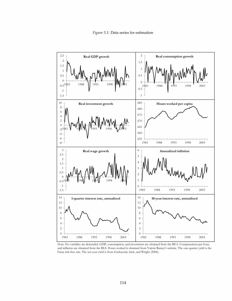
Figure 3.1: Data series for estimation

Note: No variables are detrended. GDP, consumption, and investment are obtained from the BEA. Compensation per hour,

and inflation are obtained from the BLS. Hours worked is obtained from Valerie Ramey's website. The one-quarter yield is the

Fama risk-free rate. The ten-year yield is from Gurkaynak, Sack, and Wright (2006).

-1.5

-1

-0.5

0

0.5

1

1.5

2

2.5

1983 1988 1993 1998 2003

Real GDP growth

-1

-0.5

0

0.5

1

1.5

2

1983 1988 1993 1998 2003

Real consumption growth

-8

-6

-4

-2

0

2

4

6

8

10

1983 1988 1993 1998 2003

Real investment growth

655

660

665

670

675

680

685

1983 1988 1993 1998 2003

Hours worked per capita

-1.5

-1

-0.5

0

0.5

1

1.5

2

2.5

3

1983 1988 1993 1998 2003

Real wage growth

0

1

2

3

4

5

6

1983 1988 1993 1998 2003

Annualized inflation

0

2

4

6

8

10

12

14

1983 1988 1993 1998 2003

1-quarter interest rate, annualized

0

2

4

6

8

10

12

14

1983 1988 1993 1998 2003

10-year interest rate, annualized

114

of these measurement errors is another parameter that will be estimated. The assumption

of zero measurement error for the long and short ends of the yield curve forces the model

to focus on matching the term spread, while leaving some flexibility in matching curvature.

3.5.2 Priors

Table 3.1 lists the parameters and priors. For all of the parameters that I share with JPT,

I choose the same priors. The remaining parameters are listed in the bottom section of the

table. Many of them have uniform priors since I do not have strong a priori views about,

for example, the fraction of the variance of the Federal Reserve’s inflation target that is

driven by shocks to government spending.

For the volatility of risk aversion, I choose a beta distribution over the ratio of the un-

conditional standard deviation of risk aversion to its mean. This means that average risk

aversion is forced to be at least one standard deviation above zero. This prior could po-

tentially be tightened to enforce a stronger restriction. As a practical matter, the data tends

to push for a high volatility for risk aversion, and average risk aversion in the estimation

simply rises high enough to accommodate the unconditional standard deviation.

I constrain the persistence of the inflation target to follow nearly a random walk with

ρπ∗ = 0.99, consistent with the idea that the target is highly persistent. The assumption

that ρπ∗ < 1 ensures that inflation is stationary so that there is a steady-state around which

we can approximate. The priors over the shares of the variances of the inflation target and

risk aversion coming from the other shocks are uniform.

3.5.3 Posterior modes

Table 3.1 lists the posterior modes for the parameters along with the 5th and 95th per-

centiles of the posterior distribution. Many of the posterior modes are reasonably close to

the corresponding prior means. I focus mainly on those parameters that differ from the

prior or are unique to this model.

The prior for the variance of the innovations to the inflation target favors a reason-

ably low standard deviation, but the posterior seems to want a highly volatile target—the

115

Table 3.1: Priors and posterior modes

Estimates

Description Distribution Mean Std. Dev. Mode 5% 95% from JPT

1 α Capital share Normal 0.3 0.05 0.13 0.10 0.15 0.172 ιp Price indexation Beta 0.5 0.15 0.39 0.21 0.56 0.24

3 ιw Wage indexation Beta 0.5 0.15 0.77 0.66 0.88 0.11

4 100γ Mean technology growth Normal 0.5 0.25 0.48 0.43 0.52 0.48

5 η Habit parameter Beta 0.5 0.1 0.52 0.32 0.71 0.786 λp Mean price markup Normal 0.15 0.05 0.10 0.02 0.18 0.23

7 λw Mean wage markup Normal 0.15 0.05 0.15 0.07 0.24 0.15

8 LSS Mean log hours per capita Normal 6.7 0.2 6.75 6.71 6.79 N/A

9 πSS Mean quarterly inflation Normal 0.5 0.1 -0.20 -0.90 0.74 0.71

10 100(β-1

-1) Discount factor Gamma 0.25 0.1 0.28 0.21 0.47 0.13

11 ν Inverse Frisch elasticity Gamma 2 0.75 1.83 1.16 2.87 3.7912 ξp Price adjustment frequency Beta 0.66 0.1 0.67 0.60 0.71 0.84

13 ξw Wage adjustment frequency Beta 0.66 0.1 0.67 0.57 0.72 0.7

14 χ Capital utilization costs Gamma 5 1 5.08 3.23 7.19 5.3

15 S Investment adjustment costs Gamma 4 1 4.96 3.16 6.71 2.8516 fπ Taylor rule inflation Normal 1.7 0.3 1.89 1.51 2.51 2.09

17 fy Taylor rule output gap Gamma 0.125 0.04 0.08 0.04 0.16 0.07

18 f∆y Taylor rule output gap growth Normal 0.125 0.05 0.25 0.21 0.30 0.24

19 ρR Interest rate smoothing Beta 0.6 0.2 0.96 0.92 0.97 0.82

20 ρz Technology shock AR Beta 0.6 0.2 0.20 0.09 0.31 0.23

21 ρg Government spending AR Beta 0.6 0.2 0.99 0.99 0.99 0.99

22 ρµ Investment technology AR Beta 0.6 0.2 0.50 0.34 0.67 0.72

23 ρλp Price markup AR Beta 0.6 0.2 0.95 0.92 0.97 0.94

24 ρλw Wage markup AR Beta 0.6 0.2 0.99 0.99 0.99 0.97

25 ρb Consumption demand shock AR Beta 0.6 0.2 0.77 0.70 0.80 0.67

26 ρmp Monetary policy AR Beta 0.4 0.2 0.19 0.09 0.30 0.14

27 θp Price markup MA Beta 0.5 0.2 0.16 0.02 0.39 0.77

28 θw Wage markup MA Beta 0.5 0.2 0.98 0.97 0.98 0.91

29 σR MP shock vol. IG(1) 0.1 1 0.14 0.12 0.17 0.22

30 σz Neutral tech. shock vol. IG(1) 0.5 1 0.80 0.69 0.97 0.88

31 σg Gov't spending vol. IG(1) 0.5 1 0.29 0.25 0.35 0.35

32 σµ Investment tech. vol. IG(1) 0.5 1 6.21 3.76 9.39 6.03

33 σλp Price markup vol. IG(1) 0.1 1 0.12 0.10 0.18 0.14

34 σλw Wage markup vol. IG(1) 0.1 1 0.35 0.30 0.43 0.2

35 σb Demand shock vol. IG(1) 1 1 0.41 0.29 0.63 0.04

36 σπ* Inflation target vol. IG(1) 0.1 0.1 0.33 0.28 0.41 N/A

37 σπ*,mp MP var. shr. in pi* U[-1,1] 0 0.58 0.39 0.19 0.48 N/A

38 σπ*,z z var. shr. in pi* U[-1,1] 0 0.58 -0.16 -0.26 -0.12 N/A

39 σπ*,g g var. shr. in pi* U[-1,1] 0 0.58 0.00 0.00 0.01 N/A

40 σπ*,µ mu var. shr. in pi* U[-1,1] 0 0.58 0.01 0.00 0.04 N/A

41 σπ*,λp Price shock var. shr. in pi* U[-1,1] 0 0.58 -0.04 -0.10 -0.01 N/A

42 σπ*,λw Wage shock var. shr. in pi* U[-1,1] 0 0.58 -0.06 -0.12 -0.01 N/A

43 σπ*,b b var. shr. in pi* U[-1,1] 0 0.58 0.28 0.18 0.40 N/A

44 σα/αSS RRA volatility/RRA mean Beta 0.5 0.2 0.95 0.83 0.99 N/A

45 σα,z z var. shr. in RRA U[-1,1] 0 0.58 0.00 -0.03 0.05 N/A

46 ρα RRA persistence U[-1,1] 0.5 0.29 0.77 0.72 0.83 N/A

47 ρ Inverse EIS U[-1,1] 0.5 0.29 0.76 0.51 0.90 148 αSS Mean risk aversion Normal 15 5 18.70 13.42 26.57 1

49 σyields Bond measurement errors (bp) IG(1) 13 33 8.20 7.66 8.96 N/A

Priors Posterior

Note: Priors, posterior mode, and percentiles of the posterior distribution from the benchmark model. The far-right column reports the

parameters from JPT, where applicable.

116

estimated standard deviation of the innovations to the annualized inflation target is 1.3

percent. This helps the model capture the observed volatility of the level factor in bond

yields, but it is implausibly high.

The shock to the level of labor-neutral technology has an important effect on the in-

flation target, accounting for 16 percent of the variance of its innovations. Following a

positive innovation to technology, the central bank is estimated to lower its inflation tar-

get, consistent with the idea that following beneficial supply shocks that drive inflation

downward, the central bank takes the opportunity to drive inflation lower persistently

(e.g. Gurkaynak, Sack, and Swanson, 2005). This mechanism will turn out to be critical to

the main results.

The labor-neutral technology shock has a standard deviation of 0.72 and an autocorre-

lation of 0.22. The permanent component of the technology process (the Beveridge–Nelson

trend) thus has a standard deviation of 1.00, which is similar to the values often calibrated

in the production-based asset pricing literature (e.g. Gourio, 2010, and Dew-Becker, 2011a).

The estimated long-run variance of technology growth is far smaller than the value cali-

brated in the long-run risks literature (e.g. Bansal and Yaron, 2004, and Kaltenbrunner

and Lochstoer, 2010), but it is consistent with estimates obtained in JPT and SW and with

simple univariate estimates from consumption and output data.

The standard deviation of the investment technology shock is far larger than the prior,

which is also consistent with JPT, showing that innovations that are isolated to the invest-

ment sector may play a large role in fluctuations. Alternatively, it could mean that the

model simply matches investment poorly.

The estimates imply that there is essentially zero correlation between innovations to

technology and innovations to risk aversion. This runs against the theory from Dew-

Becker (2011a), and implies that the price of risk in bond markets is driven by some fac-

tor other than permanent innovations to household consumption. Intuitively, part of the

source of this result is that the price of risk is measured to be high in recessions, but over

the 1983–2004 period, productivity growth has been only weakly procyclical, and in fact

rose substantially in the 2000 recession.

As in JPT, the government spending shock is estimated to follow nearly a unit root,

117

explaining the trend in the consumption-output ratio over the sample. The wage markup

shock also follows nearly a unit root, which helps capture the strong trend in hours worked

per capita seen in figure 3.1.

In general, my parameter estimates are reassuringly similar to the values from JPT re-

ported in the far-right column of table 3.1, even though I use a different sample period

(post-1983 versus post-war) and extra data on bond yields. The main place where my es-

timates seem to differ from JPT is in price and wage determination. My estimates imply

that wages are strongly indexed to inflation, whereas JPT estimate little indexation. The

wage-markup shock is also substantially more volatile under my estimates than JPT. In-

terestingly, when bond prices are dropped from the estimation, I obtain values for wage

indexation and the volatility of the wage markup shock that are much closer to JPT. This

suggests that wage dynamics are important for matching the term structure. I also esti-

mate a smaller inverse Frisch elasticity and a lower average price markup. In both cases,

my estimates bring the model in closer to the priors and micro estimates.

3.6 Asset pricing

This section studies the asset-pricing implications of the model. I first analyze the fit

of the model to the term structure and show that it is competitive with a non-structural

model. Next, I decompose the variance of the SDF to understand the source of the posi-

tive term premium in the model. I then analyze the prices of other assets, including the

aggregate capital stock and a claim to aggregate profits.

3.6.1 Bond prices

3.6.1.1 Fitted yields

Figure 3.2 plots the deviations of the fitted yields from their actual values for the five

yields that are assumed to be measured with error (reported in annualized basis points).

The estimated standard deviation of these fitting errors is 8 basis points, which is econom-

ically small compared to the overall variation of the yields that is on the order of hundreds

118

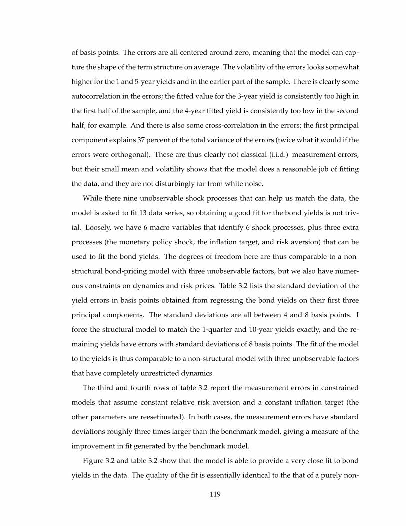
of basis points. The errors are all centered around zero, meaning that the model can cap-

ture the shape of the term structure on average. The volatility of the errors looks somewhat

higher for the 1 and 5-year yields and in the earlier part of the sample. There is clearly some

autocorrelation in the errors; the fitted value for the 3-year yield is consistently too high in

the first half of the sample, and the 4-year fitted yield is consistently too low in the second

half, for example. And there is also some cross-correlation in the errors; the first principal

component explains 37 percent of the total variance of the errors (twice what it would if the

errors were orthogonal). These are thus clearly not classical (i.i.d.) measurement errors,

but their small mean and volatility shows that the model does a reasonable job of fitting

the data, and they are not disturbingly far from white noise.

While there nine unobservable shock processes that can help us match the data, the

model is asked to fit 13 data series, so obtaining a good fit for the bond yields is not triv-

ial. Loosely, we have 6 macro variables that identify 6 shock processes, plus three extra

processes (the monetary policy shock, the inflation target, and risk aversion) that can be

used to fit the bond yields. The degrees of freedom here are thus comparable to a non-

structural bond-pricing model with three unobservable factors, but we also have numer-

ous constraints on dynamics and risk prices. Table 3.2 lists the standard deviation of the

yield errors in basis points obtained from regressing the bond yields on their first three

principal components. The standard deviations are all between 4 and 8 basis points. I

force the structural model to match the 1-quarter and 10-year yields exactly, and the re-

maining yields have errors with standard deviations of 8 basis points. The fit of the model

to the yields is thus comparable to a non-structural model with three unobservable factors

that have completely unrestricted dynamics.

The third and fourth rows of table 3.2 report the measurement errors in constrained

models that assume constant relative risk aversion and a constant inflation target (the

other parameters are reesetimated). In both cases, the measurement errors have standard

deviations roughly three times larger than the benchmark model, giving a measure of the

improvement in fit generated by the benchmark model.

Figure 3.2 and table 3.2 show that the model is able to provide a very close fit to bond

yields in the data. The quality of the fit is essentially identical to the that of a purely non-

119

Figu

re3.

2:Bo

ndyi

eld

erro

rs

Note: each axis plots the measurement errors in basis points for one of the bond yields. Errors are m

easured from the Kalman-filtered estim

ates at the posterior mode.

-30

-20

-100

10203040

1980

1990

2000

Yield errors (basis points)1-year

1980

1990

2000

2-year

1980

1990

2000

3-year

1980

1990

2000

4-year

-30

-20

-10

010203040

1980

1990

2000

Yield errosr (basis points)

5-year

120

Table 3.2: Fitting Errors

1-quarter 1-year 2-year 3-year 4-year 5-year 10-year

PCA 4.54 7.32 6.29 4.26 6.20 7.98 6.53

Benchmark model 0 8.12 8.12 8.12 8.12 8.12 0

Constant RRA 0 23.30 23.30 23.30 23.30 23.30 0

Constant π* 0 23.87 23.87 23.87 23.87 23.87 0

Note: Fitting errors measured in annualized basis points. The model-based estimates use the posterior

modal estimate for the standard deviation. The 1-quarter and 10-year errors are constrained to equal zero in

the structural model. The errors from PCA are the standard deviations of the residuals from regressions on

the bond yields on their first three principal components.

121

structural model.

3.6.1.2 Steady-state yields

Another way to evaluate the fit of the model is to ask whether the steady state of the

model matches the average term structure in the data. Looking at the steady state keeps

the Kalman filter from using large deviations in the unobservable state variables to fit

the term structure. Figure 3.3 plots the average term structure in the sample along with its

model-implied steady state. The solid black line gives the steady-state term structure in the

model, renormalized so that the ten-year yield matches the empirical ten-year yield.7 To

capture the uncertainty in the empirical term structure, the grey area gives the 95-percent

confidence intervals for the means of the empirical yields relative to the ten-year yield

(i.e. the confidence intervals for the spreads; the intervals are calculated using the Newey–

West method with lag a 6-quarter lag window). What figure 3.3 shows is that the model

matches the spread between the 10 and 2-year yields, but it does not match the curvature

of the term structure below two years. However, all of the model-implied yields are within

the 95 confidence intervals. One potential explanation at the very short end of the yield

curve is that there is a small liquidity premium that the model is not incorporating.

We will see that two features of the model are critical for generating the large steady-

state term premium: first, following a positive shock to technology, the Fed’s inflation

target falls; second, variation in risk aversion raises the premia on risky assets. To see the

prima facie evidence that these two effects are key, figure 3.3 includes two lines giving the

steady-state term structure in constrained models. The first line assumes that innovations

to the inflation target are uncorrelated with the permanent technology shock, while the

second line assumes that risk aversion is fixed. Neither line reestimates the other parame-

ters, so they simply isolate the effects of those two features of the model.

The line exiting the top of the chart is for the model when shocks to technology are

assumed to have no impact on the inflation target. We then obtain the usual result that the

term structure is downward-sloping, and the steady-state term spread is -261 basis points.

7 I use this normalization because the estimated inflation target is above zero through most of the sample.The unconditional variance of the inflation target is sufficiently high that its average level is not well identified.

122

Figu

re3.

3:St

eady

-sta

teno

min

albo

ndyi

elds

4

4.55

5.56

6.57

7.58

04

812

16

20

24

28

32

36

Annualized nominal yield (percentage points)

Maturity (quarters)

Aver

age

empir

ical

yie

lds

(spre

ad=

2.0

7)

Ste

ady-

stat

eyi

eld

s (s

pre

ad=

1.5

2)

Note

:The

solid b

lack

line

gives

the

yiel

d c

urv

e at

the

model

's s

tead

y st

ate;

the

grey

lines

are

for

the

model

wit

h c

onst

ant

risk

aver

sion a

nd w

her

e th

e in

flat

ion t

arge

t is

u

naf

fect

ed b

y sh

ock

s to

lab

or-

neu

tral

tec

hnolo

gy. T

he

oth

er p

aram

eter

s ar

e not

rees

tim

ated

. All t

he

linea

r ar

e norm

aliz

ed t

o m

atch

the

10-y

ear

yiel

d e

xact

ly, s

o t

he

plo

t m

easu

res

stea

dy-

stat

e sp

read

s. B

oxe

s ar

e av

erag

e sa

mple

yie

lds.

The

grey

are

a is

the

95%

confi

den

ce b

and

for

the

aver

age

yiel

ds

rela

tive

to t

he

10-y

ear

yiel

d, c

alcu

late

d

usi

ng

the

New

ey–W

est m

ethod

wit

h 6

lag

s. T

he

solid

bla

ck li

ne

gives

the

yiel

d c

urv

e at

the

model

's s

tead

y st

ate,

norm

aliz

ed to m

atch

the

10-y

ear

yiel

d e

xact

ly.

Ste

ady-

stat

eyi

eld

sC

onst

ant

risk

aver

sion

(spre

ad=

0.6

3)

Em

pir

ical

95%

confi

den

ce b

and

Ste

ady-

stat

eyi

eld

s π*

ind

ep. of

z(s

pre

ad=

-2.6

1)

123

Time-varying risk aversion also turns out to be important, though. When risk aversion is

fixed, the term structure is still upward-sloping, but the spread is quantitatively small—

only 63 basis points in steady-state, compared to 207 in the data and 152 in the benchmark

model.

3.6.1.3 Term premia

The size of the steady-state term spread in the model can be interpreted as the average

term premium—it is the excess return (in logs) that an investor earns in expectation by

buying a long-term bond and holding it to maturity instead of buying short-term bonds

and rolling them over for the same amount of time. An important feature of this model is

that risk aversion varies over time, which should make the term premium also vary over

time.

The top panel of figure 3.4 plots the expected annualized excess return on holding

a ten-year nominal bond (over a one-quarter bond) from the benchmark model against

the expected excess return from a regression of bond returns on the Cochrane–Piazzesi

(CP) factor. Cochrane and Piazzesi (2005) argue that a tent-shaped factor in forward yields

summarizes the price of risk in the term structure, so their factor can be viewed as a simple

non-structural benchmark for return forecasting.

The structural forecast is highly correlated (34 percent) with the fitted value using the

CP factor, and its standard deviation is roughly 20 percent larger. The two series rise

by similar amounts in the two recessions in the sample, but the benchmark model also

implies that the term premium rose in 1988 and 1999, whereas the CP factor is stable in

those episodes.

The bottom panel of figure 3.4 plots the term premium against the term spread. The

term premium is defined as the spread between the 10-year yield and the average of the

expected 1-quarter yields over the life of a 10-year bond. The variance of the term pre-

mium is non-trivial in comparison to the term spread. In the two recessions in the sample,

the increases in the term spread are substantially larger than the movements in the term

premium, but the term premium does rise in both episodes. Interestingly, the movements

124

Figure 3.4: Expected returns and the term premium

Note: Top panel gives expected excess returns on a 10-year bond over the following quarter, annualized. Values for the

Cochrane–Piazzesi are from a linear regression. The term premium in the bottom panel is defined as the gap between the 10-

year nominal yield and the mean of expected 1-quarter yields over the following 10 years.

-2

0

2

4

6

8

10

12

1983 1988 1993 1998 2003

Annualized expected return on 10-year nominal bond

Benchmark model

Cochrane–Piazessi

-1

0

1

2

3

4

5

1983 1988 1993 1998 2003

10-year/1-quarter term spread and term premium

Term spread

Term premium

125

in the term spread outside of the two recessions seem almost entirely driven by move-

ments in the term premium. In particular, the rises in the term spread in 1984, 1985, 1987,

1996, and 1999 are all associated with increases in the term premium of equal magnitudes.

On the other hand, the inversions of the yield curve in 1989 and 2000, both just prior to

recessions, are associated with only minor declines in risk aversion, and the subsequent

rises in the term spread with similarly small rises in risk aversion.

3.6.1.4 Variation in interest rates

To show how the bond yields respond to the various shocks, figure 3.5 plots responses

of a level, slope, and curvature factor to the 9 fundamental shocks. Following Bekaert, Cho,

and Moreno (2010), the level factor is defined as the average of the 1-quarter and 5 and 10-

year yields; the slope factor is the 10-year/1-quarter term spread; and curvature is the sum

of the 5 and 1-year yields minus twice the 3-year yield. The shocks are orthogonalized in

the sense that the interactions between the inflation target and risk aversion and the other

shocks are switched off. So figure 3.5 shows, for example, the effect of a pure increase in

the level of technology, holding the inflation target fixed. The shocks are all unit standard

deviations.

For the level factor, a number of shocks, the monetary policy and time preference

shocks in particular, have important effects at high frequencies. The low-frequency move-

ments, as we would expect, are mainly driven by shifts in the inflation target, while risk

aversion also plays a role. Somewhat surprisingly, positive monetary policy shocks, which

raise the short-term interest rate above its Taylor-rule value, are actually associated with

declines in the level factor. The reason is that these shocks drive down expected inflation.

So a positive monetary policy shock drives the real interest rate up, but nominal interest

rates actually fall. The response to the time-preference shock is more intuitive: an increase

in Bt is analogous to an increase in patience, so interest rates fall.

The determinants of the slope factor are similar to those for the level factor: monetary

policy and time-preference matter at high frequencies, while risk aversion determines the

dynamics at lower frequencies. An increase in risk aversion increases the term spread,

126

Figu

re3.

5:R

espo

nses

ofte

rmst

ruct

ure

fact

ors

toor

thog

onal

ized

shoc

ks

AAA

Note

: re

sponse

s of ea

ch o

f th

e te

rm struct

ure

fac

tors

to the

orthogo

nal

struct

ura

l sh

ock

s. S

pec

ific

ally

, risk

aver

sion a

nd the

inflat

ion tar

get ar

e only

aff

ecte

d b

y th

eir ow

n shock

s, n

ot th

e sh

ock

s to

the

oth

er e

xoge

nous

pro

cess

es. The

level

fac

tor is the

aver

age

of th

e 1-q

uar

ter, 5

-yea

r, a

nd 1

0-y

ear yi

elds. T

he

slope

fact

or is the

gap b

etw

een the

10-y

ear an

d 1

-quar

ter yi

elds. C

urv

ature

is th

e su

m o

f th

e 5-y

ear an

d 1

-yea

r yi

elds m

inus tw

ice

the

3-y

ear yi

eld. The

shock

s ar

e al

l unit sta

ndar

d d

evia

tions. A

ll sca

les in

eac

h row

are

iden

tica

l an

d a

re m

easu

red in a

nnual

ized

per

centa

ge p

oin

ts.

Time Preference

Inflation Target

Risk aversion

Level Factor Slope Factor Curvature factorMonetary Pol.

Neutral Tech.

Gov't Spending

Investment. Tech.

Prices

Wages

-0.4

-0.3

-0.2

-0.10

0.1

0.2

0.3

0.4

111

21

31

-0.4

-0.3

-0.2

-0.10

0.1

0.2

0.3

0.4

111

21

31

-0.4

-0.3

-0.2

-0.10

0.1

0.2

0.3

0.4

111

21

31

-0.4

-0.3

-0.2

-0.10

0.1

0.2

0.3

0.4

111

21

31

-0.4

-0.3

-0.2

-0.10

0.1

0.2

0.3

0.4

111

21

31

-0.4

-0.3

-0.2

-0.10

0.1

0.2

0.3

0.4

111

21

31

-0.4

-0.3

-0.2

-0.10

0.1

0.2

0.3

0.4

111

21

31

-0.4

-0.3

-0.2

-0.10

0.1

0.2

0.3

0.4

111

21

31

-0.4

-0.3

-0.2

-0.10

0.1

0.2

0.3

0.4

111

21

31

-0.5

-0.4

-0.3

-0.2

-0.10

0.1

0.2

0.3

0.4

0.5

0.6

0.7

0.8

111

21

31

-0.5

-0.4

-0.3

-0.2

-0.10

0.1

0.2

0.3

0.4

0.5

0.6

0.7

0.8

111

21

31

-0.5

-0.4

-0.3

-0.2

-0.10

0.1

0.2

0.3

0.4

0.5

0.6

0.7

0.8

111

21

31

-0.5

-0.4

-0.3

-0.2

-0.10

0.1

0.2

0.3

0.4

0.5

0.6

0.7

0.8

111

21

31

-0.5

-0.4

-0.3

-0.2

-0.10

0.1

0.2

0.3

0.4

0.5

0.6

0.7

0.8

111

21

31

-0.5

-0.4

-0.3

-0.2

-0.10

0.1

0.2

0.3

0.4

0.5

0.6

0.7

0.8

111

21

31

-0.5

-0.4

-0.3

-0.2

-0.10

0.1

0.2

0.3

0.4

0.5

0.6

0.7

0.8

111

21

31

-0.5

-0.4

-0.3

-0.2

-0.10

0.1

0.2

0.3

0.4

0.5

0.6

0.7

0.8

111

21

31

-0.5

-0.4

-0.3

-0.2

-0.10

0.1

0.2

0.3

0.4

0.5

0.6

0.7

0.8

111

21

31

-0.25

-0.2

-0.15

-0.1

-0.050

0.05

0.1

0.15

0.2

0.25

111

21

31

-0.25

-0.2

-0.15

-0.1

-0.050

0.05

0.1

0.15

0.2

0.25

111

21

31

-0.25

-0.2

-0.15

-0.1

-0.050

0.05

0.1

0.15

0.2

0.25

111

21

31

-0.25

-0.2

-0.15

-0.1

-0.050

0.05

0.1

0.15

0.2

0.25

111

21

31

-0.25

-0.2

-0.15

-0.1

-0.050

0.05

0.1

0.15

0.2

0.25

111

21

31

-0.25

-0.2

-0.15

-0.1

-0.050

0.05

0.1

0.15

0.2

0.25

111

21

31

-0.25

-0.2

-0.15

-0.1

-0.050

0.05

0.1

0.15

0.2

0.25

111

21

31

-0.25

-0.2

-0.15

-0.1

-0.050

0.05

0.1

0.15

0.2

0.25

111

21

31

-0.25

-0.2

-0.15

-0.1

-0.050

0.05

0.1

0.15

0.2

0.25

111

21

31

127

which fits with results on bond return forecasting (Campbell and Shiller, 1988) and the fact

that the term spread forecasts high equity returns (Fama and French, 1989).

3.6.2 Determinants of asset prices

3.6.2.1 The variance of the SDF

An asset’s expected excess return over the real riskless interest rate is determined by

its covariance with the stochastic discount factor. One of the more interesting outputs of

a model as rich as this one is the variance decomposition for the SDF. Table 3.3 reports a

variance decomposition for the SDF at the one-quarter horizon. The variance of the SDF

is essentially entirely driven by the neutral technology and risk aversion shocks. The bar

chart in the bottom panel of table 3.3 decomposes the variance of the SDF into components

coming from the neutral technology shock, the risk aversion shock, and the remaining

shocks combined. The lines at the top of each bar give the 2.5 and 97.5 percentiles of

the posterior distribution. The 97.5 percentile for the variance share in the SDF for non-

technology and non-risk-aversion shocks is less than 2 percent.

On first glance this result might be somewhat surprising, but it is in fact a deep char-

acteristic of models with Epstein–Zin preferences with a high EIS and high risk aversion.

One way to see the source of this finding is to simply look at the household’s SDF,

Mt+1 = βBt1− βBt+1

1− βBt

UC,t+1

UC,t

Vρ−αtt+1(

EtV1−αtt+1

) ρ−αt1−αt

(3.46)

For a household with a large EIS, the variance of UC,t+1/UC,t is generally small (at least

with standard preferences). In the case where the household does not have a habit (η = 0),

this term is equal to (Ct+1/Ct)−ρ. If the household has an EIS greater than 1, then ρ is less

than 1 and the variance of UC,t+1/UC,t will be less than the variance of log consumption

growth. A one-percent permanent decline in consumption will raise this term by the factor

1.01ρ.

The majority of the variance of the SDF is driven by the term Vρ−αtt+1(

EtV1−αtt+1

) ρ−αt1−αt

. Here, a one-

percent permanent decline in consumption will make this term (approximately) equal to

128

Tabl

e3.

3:O

ne-q

uart

erah

ead

vari

ance

deco

mpo

siti

ons

12

34

56

78

9

SDF

Utility return

Cons. return

Nom. lev

.

cons. ret.

Rea

l lev. cons.

ret.

10-yea

r bond

return

Output

growth

Consu

mption

growth

Inve

stmen

t

growth

1M

onetary polic

y0.00

0.00

0.00

0.00

0.00

0.34

0.00

0.00

0.00

2Neu

tral tec

h.

0.57

0.00

0.00

0.01

0.15

0.14

0.00

0.03

0.03

3Gov't sp

ending

0.00

0.00

0.00

0.00

0.00

0.00

0.09

0.07

0.00

4In

vestmen

t tech

.0.00

0.00

0.00

0.00

0.00

0.00

0.31

0.01

0.92

5Price

marku

p0.00

0.00

0.00

0.00

0.00

0.06

0.04

0.02

0.04

6W

age marku

p0.00

0.00

0.00

0.00

0.01

0.03

0.00

0.01

0.01

7Tim

e preference

0.01

0.94

0.94

0.91

0.36

0.17

0.03

0.04

0.00

8In

flation targe

t0.00

0.05

0.05

0.07

0.02

0.03

0.52

0.83

0.00

9Risk av

ersion

0.41

0.00

0.01

0.01

0.46

0.23

0.00

0.00

0.00

Moments:

10Standard dev

iation

0.47

4.06

4.06

8.67

6.54

19.65

1.19

1.07

1.91

11Correl. w

/ SDF

1.00

-0.14

-0.17

-0.09

-0.80

-0.53

0.01

0.04

-0.12

12Exp

ected return

N/A

0.27

0.33

0.36

2.47

4.90

N/A

N/A

N/A

Note: d

ecompositions of one-quarter ah

ead foreca

st error. L

evered

return

s fo

r ca

pital and consu

mption claim

s assu

me that the inve

stor finan

ces half the purchase price

of the

give

n claim

with a 10-ye

ar nominally riskless bond. T

he 10

-yea

r return

is the one-quarter return

fro

m holding a 10

-yea

r nominally riskless bond. T

he momen

ts in rows 10–12

are

annualized

. The black

bars in the figu

re give the 95

perce

nt cred

ible reg

ion based

on ran

dom draws from the posterior den

sity.

0.00

0.10

0.20

0.30

0.40

0.50

0.60

0.70

0.80

0.90

1.00

SDF

Utility return

Cons. return

Lev

ered

cons. ret.

LR cons. ret.

10-year bond

return

Output growth

Consu

mption

growth

Inve

stmen

t growth

Variance decompositions and 95% credible intervals

Neu

tral

tech

nology

Risk av

ersion

All other

shock

s

129

1.01αt−ρ. When αt � ρ, as estimated here and in most models with Epstein–Zin prefer-

ences, it is therefore the variation in Vt+1 that determines the behavior of the SDF.

So what determines movements in Vt+1? One way to think about it is to split move-

ments in consumption into permanent and temporary components. A purely temporary

shock to consumption will have a relatively small impact on Vt+1 because the household is

not very averse to shifting consumption over time. A permanent shock to consumption, on

the other hand, will tend to shift Vt+1 by an equal amount. Risk aversion shocks also affect

Vt. The reason is simply that increases in risk aversion directly drive Vt+1 down because

households are more averse to the future uncertainty that they face. Since it is the shocks

to Vt+1 that determine the movements in Mt+1, we should thus not be surprised that it is

mainly the neutral technology and risk aversion shocks that drive the variance of the SDF.

3.6.2.2 Impulse responses

Since the technology and risk aversion shocks are the key to understanding the pricing

kernel, it is natural to ask how they affect the economy. Figure 3.6 plots impulse responses

to an increase in labor-neutral technology and a decrease in risk aversion. Dotted lines give

95-percent credible intervals (the range between the 2.5 and 97.5 percentiles in the posterior

distribution). These impulse responses are different from those in figure 3.5 because they

do not turn off the interactions between the inflation target and risk aversion and the other

shocks. The idea is that we want to see what happens on average following these two

shocks, since that behavior is what is relevant for understanding the correlations with the

SDF.

Following the technology shock, inflation falls, while output and real interest rates

rise: a standard positive supply shock. The declines in inflation and nominal interest rates

are especially pronounced and persistent. This behavior is the result of the fact that the

estimates imply that the inflation target falls following an increase in technology. However,

note that inflation falls more than the inflation target does, so the effect is not entirely

driven by the inflation target.

A similar result is obtained in JPT and SW, even though they do not have time-varying

130

Figure 3.6: Responses to technology and risk-aversion shocks

Note: responses in percentage points to a unit standard deviation positive shock to labor-neutral technology and a negative shock to risk aversion. Interest rate,

inflation, and inflation target are annualized. Dotted lines give 2.5 and 97.5 percentiles from the posterior distribution

-0.9

-0.7

-0.5

-0.3

-0.1

0.1

0.3

0 5 10 15 20

Nominal risk-free rate

Increase inlabor-neutral technology

Decline in risk aversion

-0.1

0

0.1

0.2

0.3

0.4

0.5

0.6

0 5 10 15 20

Real risk-free rate

-1.4

-1.2

-1

-0.8

-0.6

-0.4

-0.2

0

0.2

0.4

0 5 10 15 20

Inflation

Decline in risk aversion

Increase in labor-neutral technology

-1.2

-1

-0.8

-0.6

-0.4

-0.2

0

0.2

0.4

0 5 10 15 20

Inflation target

-0.6

-0.4

-0.2

1E-15

0.2

0.4

0.6

0.8

1

1.2

0 5 10 15 20

Output

Decline in risk aversion

Increase in labor-neutral technology

-0.7

-0.5

-0.3

-0.1

0.1

0.3

0 5 10 15 20

Output gap

95-percent credibleinterval

131

inflation targets. In all of these models, because prices are sticky, when there is a positive

supply shock, rather than cutting prices, firms simply produce the same quantity as previ-

ously, thereby reducing employment and hence demand. Positive technology shocks are

thus associated with small increases in output and large declines in the output gap (de-

fined as the difference between output and the level it would take if prices were flexible).

There is also a small empirical literature that provides more reduced-form evidence on

effects of this sort using direct measures of technology (e.g. Basu, Fernald, and Kimball,

2006).

The slow response of output to a technology shock is particularly notable. The impulse

response function in figure 3.6 suggests that output and perhaps also consumption growth

should be predictable and positively autocorrelated, though other shocks could obscure

those relationships. Figure 3.7 therefore plots the empirical and model-predicted autocor-

relation functions for consumption and output growth. For output, the model implies that

the 1-quarter autocorrelation should be 0.50, while it is only 0.33 in the data. But 0.50 is

well within the 95 percent confidence interval for the empirical value. In fact, nearly the

entire autocorrelation function for output in the model is captured within the 95 percent

confidence interval in the data.

The model also implies strong one-quarter autocorrelation in consumption growth, and

the autocorrelation is in fact higher than the upper end of the 95 percent confidence in-

terval. However, this autocorrelation dies out very rapidly, and at lags longer than one

quarter the autocorrelation of consumption growth in the model matches the behavior in

the data well. The model implies little or no serial correlation in consumption and output

growth at horizons longer than two quarters.

Figure 3.6 also reports impulse responses for a decline in risk aversion. Inflation, in-

terest rates, and the output gap all rise. This shock therefore takes the form of a classic

demand shock. The effects are far smaller than those for the technology shock. Risk aver-

sion has two main channels through which it affects the real economy. First, to the extent

that physical investment is risky, a decline in risk aversion makes households more will-

ing to purchase physical capital. Second, a decline in precautionary saving demand makes

households want to consume more for any given level of interest rates. For this model,

132

Figure 3.7: Empirical and model-implied autocorrelations

Notes: Empirical and model-implied autocorrelation functions. Gray regions are 95-percent confidence intervals

-0.8

-0.6

-0.4

-0.2

0

0.2

0.4

0.6

0.8

1 6 11 16 21 26 31 36

Output growth

Model

-0.6

-0.4

-0.2

1E-15

0.2

0.4

0.6

1 6 11 16 21 26 31 36

Consumption growth

Empirical

Empirical 95 %confidence band

133

the increase in consumption demand dominates, which is why the shock is slightly expan-

sionary.

3.6.2.3 Other asset prices

Variance decompositions After the SDF, table 3.3 reports variance decompositions for the

returns on a number of assets. The bottom panel of table 3.3 reports the fraction of the

variance of the one-quarter innovation to each return coming from the neutral technology

shock, the risk aversion shock, and all other shocks combined.

Column 2 reports the variance decomposition for the return on the utility portfolio. 87

percent of its variance comes from the time-preference shock. The reason is simply that the

utility claim has a relatively long duration, like that of a consol with a coupon that grows

at the average rate of the economy, so shifts in real interest rates have a large effect on its

price. The time-preference shock mainly affects real interest rates, so it drives the variance

of the utility claim. Row 11 shows that the correlation of the utility return with the SDF is

-0.14

More interestingly, the third and fourth columns of table 3.3 report variance decompo-

sitions for a claim on aggregate profits and the same claim levered two to one on short-term

nominal debt.8 Once again, little of the variance of the return is driven by the technology

or risk aversion shocks. While the neutral technology shock does play a role, it is relatively

small; the vast majority of the variation is driven by shifts in the rate of time preference due

to its effects on real interest rates. Assuming that equity is levered on nominal riskless debt

does not change this result because the returns on nominal bonds are generally unaffected

by the time-preference shock. However, column 5 shows that if equity claims are levered

on real debt, then they because highly correlated with the pricing kernel, and the model

can actually generate a large equity premium (though one that is still too small by half).

The reason is that when the firm is levered on real bonds, the effects of time-preference

shocks on the unlevered dividend claim and real bond prices cancel each other out.

8 The profits are those earned by the intermediate-good producers, Yt −Wt Nt.

134

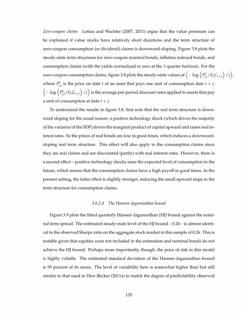
Zero-coupon claims Lettau and Wachter (2007, 2011) argue that the value premium can

be explained if value stocks have relatively short durations and the term structure of

zero-coupon consumption (or dividend) claims is downward-sloping. Figure 3.8 plots the

steady-state term structures for zero-coupon nominal bonds, inflation indexed bonds, and

consumption claims (with the yields normalized to zero at the 1-quarter horizon). For the

zero-coupon consumption claims, figure 3.8 plots the steady-state values of(− log

(PC

j,t/EtCt+j

)/j)

,

where PCj,t is the price on date t of an asset that pays one unit of consumption date t + j.(

− log(

PCj,t/EtCt+j

)/j)

is the average per-period discount rates applied to assets that pay

a unit of consumption at date t + j.

To understand the results in figure 3.8, first note that the real term structure is down-

ward sloping for the usual reason: a positive technology shock (which drives the majority

of the variance of the SDF) drives the marginal product of capital upward and raises real in-

terest rates. So the prices of real bonds are low in good times, which induces a downward-

sloping real term structure. This effect will also apply to the consumption claims since

they are real claims and are discounted (partly) with real interest rates. However, there is

a second effect – positive technology shocks raise the expected level of consumption in the

future, which means that the consumption claims have a high payoff in good times. In the

present setting, the latter effect is slightly stronger, inducing the small upward slope in the

term structure for consumption claims.

3.6.2.4 The Hansen–Jagannathan bound

Figure 3.9 plots the fitted quarterly Hansen–Jagannathan (HJ) bound against the nomi-

nal term spread. The estimated steady-state level of the HJ bound – 0.24 – is almost identi-

cal to the observed Sharpe ratio on the aggregate stock market in this sample of 0.26. This is

notable given that equities were not included in the estimation and nominal bonds do not

achieve the HJ bound. Perhaps more importantly, though, the price of risk in this model

is highly volatile. The estimated standard deviation of the Hansen–Jagannathan bound

is 95 percent of its mean. The level of variability here is somewhat higher than but still

similar to that used in Dew-Becker (2011a) to match the degree of predictability observed

135

Figu

re3.

8:St

eady

-sta

tete

rmst

ruct

ures

-1.5-1

-0.50

0.51

1.52

16

11

16

21

26

31

36

Nominal

bonds

Real bonds

Consumption

claims

Notes: term structuresfor nominal and real zero-coupon bonds and zero coupon consumption claim

s. Horizons are measured in quarters.

136

for aggregate stock returns in the post-war sample.

3.7 The real economy

Up to now, the analysis has focused mainly on asset pricing. But the model gives a

rich description of the real side of the economy. While I leave a deeper analysis of New

Keynesian models to papers focused on those models for their own sake, the interaction of

the real side of the economy with asset prices is important to this paper.

Figure 3.10 gives a variance decomposition for the variables used in the estimation.

The figure decomposes the variance of each variable at frequencies of 6 to 32 quarters into

components coming from each of the structural shocks.9 Except for investment growth, for

which the investment-specific shock is completely dominant, none of the other variables

examined in figure 3.10 are dominated by any particular shock. Notably, the shock to risk

aversion has almost no effect on the variance of any of the real variables at business-cycle

frequencies. Its largest effect is on consumption growth, for which the variance share is

still only 4 percent. The far-right bar, though, shows that risk aversion has a large effect on

the term spread, as we saw in figure 3.5; it explains roughly 1/3 of the variance of the term

spread at business-cycle frequencies.

The variance decomposition reported in the top panel of figure 3.10 is rather different

from that reported by JPT. They found that the investment shock was an important deter-

minant of not only investment, but also output and consumption growth at business-cycle

frequencies. Their model differs from mine in three ways: risk aversion and the inflation

target are constant, the preference specification is slightly different (log utility and additive

habits), and the data sample covers the entire post-war period and only includes the one-

quarter nominal interest rate. The bottom panel of figure 3.8 removes a number of those

differences. It drops bond yields (except the short rate) from the estimation and assumes

9 The variance decomposition is calculated using a spectral decomposition of the state-space form of themodel. Specifically, since the structural shocks are orthogonal, the spectral density of the endogenous vari-ables is equal to the sum of the densities obtained when each shock is turned on individually. Calculatingvariance shares over certain frequencies then simply requires integrating the density over those frequencies. Inumerically integrate by calculating the spectral density at 100 increments between wavelengths of 6 and 32quarters.

137

Figu

re3.

9:Th

eH

anse

n–Ja

gann

atha

nbo

und

and

the

term

spre

ad

00.1

0.2

0.3

0.4

0.5

0.6

0.7

-1012345

1983

1988

1993

1998

2003

Hansen–Jagannathan bound

Term spread

Term spread

Hansen

–Jagannathan

bound

138

Figure 3.10: Variance decompositions at business-cycle frequencies

Note: each section of a bar represents a fraction of the variance of one of the series at frequencies between 6 and 32 quarters.

The top panel gives results for the benchmark model. The bottom panel report results where the inflation target and risk

aversion are fixed and bond prices are dropped from the estimation. That latter model is identical to JPT except that it uses

post-1983 data and uses Epstein–Zin preferences.

0%

10%

20%

30%

40%

50%

60%

70%

80%

90%

100%Benchmark model

Risk aversion

Inflation target

Time preferenceWage markup

Price markup

Investment technologyGovernment spendingNeutral technologyMonetary policy

0%

10%

20%

30%

40%

50%

60%

70%

80%

90%

100%

JPT model

Time preference

Wage markup

Price markup

Investment technology

Government spending

Neutral technology

Monetary policy

139

the inflation target and coefficient of relative risk aversion are constant. The model is then

reestimated.

While I do not replicate JPT’s results exactly, I do also find that the investment tech-

nology shock is important for more variables than just investment itself. It accounts for 30

percent of the variation in output growth and 20 percent of consumption growth. More-

over, it accounts for 41 and 48 percent of the variance of the one-quarter nominal interest

rate and the term spread, respectively. It is this latter result that explains the divergence

between the two models. Since long-term bond prices are included in the estimation of the

benchmark model, that model is forced to match the relationship between investment and

the term spread. The difference in the variance decompositions suggests that JPT gets this

relationship wrong. What is interesting, though, is that when the model is forced to match

long-term bond yields, that also changes the decomposition for other variables.

Table 3.3 gives one-quarter-ahead variance decompositions for output, consumption,

and investment growth. This decomposition is useful for understanding whether any of

these variables would be powerful asset pricing factors. Specifically, in a world where

consumption followed a random walk and households had Epstein–Zin preferences with

constant relative risk aversion, consumption growth would be perfectly correlated with

the SDF, so it would price assets in the economy.

What table 3.3 shows is that consumption, output, and investment growth are all only

weakly correlated with the SDF at the one-quarter horizon—they all have correlations less

than 16 percent. So asset pricing with only consumption growth will not work well in

this economy. Many asset-pricing studies with Epstein–Zin preferences include both con-

sumption growth and the return on the stock market as pricing factors. If we believe that

the stock market is a claim on aggregate capital, then table 3.3 shows that it will do little to

help with asset pricing as it is also only weakly correlated with the SDF.

3.7.1 Model comparison

The primary difference between the model studied here and JPT is the addition of

time-varying risk aversion and the time-varying inflation target. An important question,

140

then, is the extent to which those two factors improve the fit of the model to the data.

Clearly, allowing a time-varying inflation target will help increase the volatility of long-

term bond yields, and time-varying risk aversion will induce time-varying risk premia.

But it is possible that the data can be well explained with a constant risk premium, or

perhaps there is no need to have a time-varying inflation target.

Table 3.4 considers two alternatives to the benchmark model: a version where the in-

flation target is constant, and a version where the coefficient of relative risk aversion is

constant. It lists two statistics for each model. First, it gives the standard likelihood ratio

used in MLE, i.e. based on log f (y|θ, M), the likelihood of the data conditional on the

model and parameters, where y represents the data and θ the parameter vector. M denotes

the model choice, i.e. the full model or one of the two restricted versions. log f (y|θ, M)

is closely related to the one-step-ahead forecast error of the model. The likelihood ratio

test favors the benchmark over each alternative by a wide margin. One way to see the

source of this rejection is to note that in table 3.2, the measurement errors for bond yields,

essentially a residual variance, are three times higher in the alternative models than the

benchmark. This difference alone is more than sufficient to explain the magnitude of the

likelihood ratios.

The second statistic is the Bayes factor, which is based on the marginal likelihood

conditional only on the model, log f (y|M) (in the economics literature, see Fernandez-

Villaverde and Rubio-Ramirez, 2004). I calculate log f (y|M) using the monte carlo chain

as in Fernandez-Villaverde and Rubio-Ramirez (2004).10

The difference in the Bayes factors listed in the bottom row of table 3.4 is similar to

the values obtained under the usual likelihood ratio test. In order to accept the model

with constant risk aversion or a constant inflation target, the ratio of the prior probabil-

ity of either of those models to that of the benchmark model would have to be greater

than exp (140). In a statistical sense, then, both the time-varying inflation target and time-

varying risk aversion substantially improve the fit of the model.

The last exercise I perform is to compare forecasting power between the structural

10 See also Gelfand and Dey (1994) and Geweke (1999)

141

Table 3.4: Model comparison statistics

Constant RRA Constant π*

Likelihood ratio 185.6 183.8

p-value 5.0E-41 1.6E-35

Bayes factor 141.50 142.50Note: Row 1 gives the marginal likelihood of the data given the model and parameters. Row

two gives the p-value for the frequentist LR test. Row 3 is the Bayes factor, the marginal

probability of the data conditional on the model (i.e. integrated over the parameter space).

142

model and a VAR. Rather than include all 13 of the endogenous variables, I use the 6

macro variables and the first three principal components of the bond yields (i.e. I estimate

a FAVAR). I estimate a VAR(2) with the restriction that the macro variables and the interest

rate factors for not interact with eachother (though their innovations may be correlated).

This assumption partly helps to limit the number of free parameters in the VAR, but it

also means that we can compare the forecasting performance of the structural model to

the benchmark models from the macro and asset-pricing literatures.

Figure 3.11 plots root mean squared errors for the forecasts from the VAR(2) and the

structural model. All of the variables are forecasted in levels, rather than differences. Be-

cause the strutural model is so difficult to estimate, I only consider in-sample forecasting

performance. For the macro variables, the structural model has somewhat weaker fore-

casting power than the VAR. The place where the divergence is notable is for inflation. At

long horizons, the structural model essentially says that the level factor in interest rates

should equal expected inflation since they are both driven by the Fed’s inflation target.

Over this sample, however, the level factor fell slowly, while inflation fell rapidly in the

early 1980’s and then was low and stable. Forecasting long-term inflation with the level

factor in this sample was thus unsuccessful compared to a simple random-walk forecast

for inflation (which is basicaly what the VAR implies).

For the bond yields, the structural model forecasts well. At long horizons, the RMSE

generated by the structural model is smaller than the VAR by 10–50 percent, with the

largest improvements coming for long-term bonds.

3.8 Conclusion

This paper studies bond pricing in a medium-scale New-Keynesian model with a time-

varying price of risk. I show that the model can generate a large and volatile term pre-

mium. The term premium is driven by the combination of two factors—a negative re-

sponse of interest rates to positive technology shocks and variation in risk aversion. Re-

moving either of these effects eliminates the model’s ability to match the magnitude of the

term premium.

143

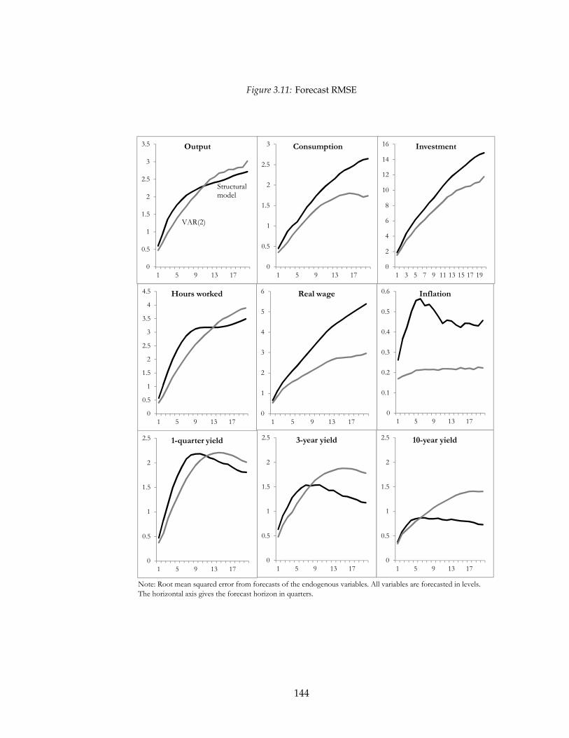
Figure 3.11: Forecast RMSE

Note: Root mean squared error from forecasts of the endogenous variables. All variables are forecasted in levels.

The horizontal axis gives the forecast horizon in quarters.

0

0.5

1

1.5

2

2.5

3

3.5

1 5 9 13 17

Output

VAR(2)

Structuralmodel

0

0.5

1

1.5

2

2.5

3

1 5 9 13 17

Consumption

0

2

4

6

8

10

12

14

16

1 3 5 7 9 11 13 15 17 19

Investment

0

0.5

1

1.5

2

2.5

3

3.5

4

4.5

1 5 9 13 17

Hours worked

0

1

2

3

4

5

6

1 5 9 13 17

Real wage

0

0.1

0.2

0.3

0.4

0.5

0.6

1 5 9 13 17

Inflation

0

0.5

1

1.5

2

2.5

1 5 9 13 17

1-quarter yield

0

0.5

1

1.5

2

2.5

1 5 9 13 17

3-year yield

0

0.5

1

1.5

2

2.5

1 5 9 13 17

10-year yield

144

While shocks to risk aversion and technology determine average asset returns, they

have only weak effects on real variables at business-cycle frequencies. The covariance

of asset returns with real variables over the business cycle is therefore unimportant for

determining average returns. It is true that the Federal Reserve tends to cut interest rates

in recessions, but the model shows that most recessions are not high-marginal-utility states

of the world. So the usual intuition that the Taylor rule should lead to a downward-sloping

yield curve is inaccurate since it does not take into the difference between the shocks that

have high risk prices and the shocks that drive the business cycle.

Furthermore, while risk aversion is estimated to be highly volatile and to be an impor-

tant determinant of the dynamics of the term spread, it has almost no effects on the real

economy. This model thus suggests that there is a separation between the price of risk in

financial markets and the real economy.

145

APPENDIX

146

A. APPENDIX TO CHAPTER 1

A.1 The approximation for average duration

Now using the investment function from the text, we have

Iit = exp (γ log (η1i) + γ (µt+1 − rt+1) + γ log Bit + log (1 + exp (µt+2 − rt+2) (1− δi)))

(A.1)

= exp (γ (µt+1 − rt+1)) exp (γ log (η1i) + γ log Bit + log (1 + exp (µt+2 − rt+2) (1− δi)))

(A.2)

Using the definition of Dt and the investment function, we have

Dt = ∑i

exp (γ log η1i + γ log Bit + log (1 + exp (µt+2 − rt+2) (1− δi)))

∑i exp (γ log η1i + γ log Bit + log (1 + exp (µt+2 − rt+2) (1− δi)))D (δi) (A.3)

Now we take a linear approximation to

exp (γ log η1i + γ log Bit + log (1 + exp (µt+2 − rt+2) (1− δi))) (A.4)

around the point{

log η1, log Bt, δ}

where log η1 ≡ ∑i log η1i, log Bt ≡ ∑i log Bit, and δ ≡

∑i δi. Also define

log (η1i) ≡ log (η1i)− log η1i

log (Bit) ≡ log (Bit)− log Bt

δi ≡ δi − δ

147

We have

exp (γ log η1i + γ log Bit + log (1 + exp (µt+2 − rt+2) (1− δi)))

≈ exp(

γlog η1i + γlog Bit + log(1 + exp (µt+2 − rt+2)

(1− δ

)))×

1 + γ log (η1i) + γ log (Bit)

−δiexp(µt+2−rt+2)

1+exp(µt+2−rt+2)(1−δ)

(A.5)

Simple algebra and the observation that

∑i

(1 + γ log (η1i) + γ log (Bit)− δi

exp (µt+2 − rt+2)

1 + exp (µt+2 − rt+2)(1− δ

)) = N (A.6)

yields the result

Dt ≈ N−1 ∑i

1 + γ log (η1i) + γ log (Bit)

− exp(µt+2−rt+2)

1+exp(µt+2−rt+2)(1−δ)δi

Di (A.7)

= N−1 ∑i

(1 + γ log (η1i) + γ log (Bit)

)Di −

exp (µt+2 − rt+2)

1 + exp (µt+2 − rt+2)(1− δ

)N−1 ∑i

δiDi

(A.8)

The term N−1 ∑i

(1 + γ log (η1i)

)Di is constant over time, and we thus have the desired

result from the text.

A.2 Further robustness tests

This section describes table A.1, which has extra robustness tests for the regressions of

D on the term spread and other controls. Column 1 includes up to three lags of the term

spread. The second lag enters significantly, and with a coefficient slightly larger than the

first lag. This sort of lagged response to price changes is commonly found in the litera-

ture. It is generally interpreted as being due to planning and delivery lags. The second

column includes every one of the other controls simultaneously, instead of individually as

in tables 2 and 3. The result is that the coefficients on the various other controls all become

marginally significant at best, while the term spread is still highly significant. There is thus

148

Figure A.1: Further robustness tests

(1) (2) (3) (4)

Term Spread(t-1) -0.23 ** -0.40 *** -0.46 *** -0.57 ***

[0.10] [0.06] [0.08] [0.09]

Term Spread(t-2) -0.24 *** -0.27 ***

[0.08] [0.08]

Term Spread(t-3) 0.11 0.12

[0.09] [0.07]

Unemployment(t-1) 0.18 0.02

[0.19] [0.20]

GDP(t) -0.05 0.02

[0.12] [0.13]

GDP(t-1) 0.36 *** 0.55 * -0.24

[0.10] [0.26] [0.22]

Investment(t) -0.08 -0.24

[0.17] [0.16]

Investment(t-1) -0.12 0.06

[0.21] [0.19]

SD_returns(t+1) -0.23 ** -0.19 ** -0.28 ***

[0.09] [0.09] [0.07]

SD_returns(t) 0.15 **

[0.07]

SD_returns(t-1) -0.08

[0.05]

N 59 47 47 45

R2 0.48 0.74 0.69 0.56Note: See tables 2 and 3.

something different about the term spread from all of the other business cycle, volatility,

and investment controls. Column 3 is identical to column 2 except it only uses one lag of

the term spread, and the coefficient is still significant at the one percent level.

Finally, column 4 includes the current and lagged values of volatility instead of just the

leading value. The leading value has a negative sign, indicating that high future volatility

lowers duration today (consistent with a model of irreversible investment). The current

value has a positive sign. One way to reconcile this is if the volatility variable should

actually enter as a first difference: an increase in volatility lowers average duration, instead

of a high value by itself. The lagged level of volatility is uncorrelated with Dt.

149

B. APPENDIX TO CHAPTER 2

B.1 The certainty equivalent

This section looks at the relationship between the certainty equivalents using Ghabit

and GTV . I first show that the two certainty equivalents are equal up to a second order

approximation around the non-stochastic version of the model. Next, I show that in the

continuous-time limit, the preferences associated with the two certainty equivalents are

identical.

B.1.1 Second-order approximation

This section approximates the certainty equivalent G−1 (Et (G (Vt+1))) where Vt+1 =

Vt × (1 + σεt+1) around the point σ = 0. We assume that Etεt+1 = 0 and Etε2t+1 = 1.

Now consider the derivative of G−1 (Et (G (Vt+1))) with respect to σ,

ddσ

G−1 (Et (G (Vt+1))) =d

dσ Et (G (Vt+1))

G′ (G−1 (Et (G (Vt+1))))(B.1)

We haved

dσEt (G (Vt+1)) =

ˆG′ (Vt (1 + σεt+1)) εt+1VtdF (εt+1) (B.2)

where F is the cdf of εt+1. Evaluated at σ = 0, ddσ Et (G (Vt+1)) = 0, and therefore

ddσ

G−1 (Et (G (Vt+1))) = 0 (B.3)

So all certainty equivalents taking this form are identical up to the first order in approxi-

mations around σ.

150

Next, consider the second derivative,

d2

dσ2 G−1 (Et (G (Vt+1))) =

[G′(G−1 (Et (G (Vt+1)))

)] d2

dσ2 Et (G (Vt+1))

−[

ddσ Et (G (Vt+1))

] [d

dσ G′(G−1 (Et (G (Vt+1)))

)][G′ (G−1 (Et (G (Vt+1))))]

2 (B.4)

Since ddσ Et (G (Vt+1)) is equal to zero at σ = 0, we can ignore the second term in the nu-

merator. The second derivative of the expectation is

d2

dσ2 Et (G (Vt+1)) =

ˆG′′ (Vt (1 + σεt+1)) ε2

t+1V2t dF (εt+1) (B.5)

At σ = 0, d2

dσ2 Et (G (Vt+1))∣∣∣σ=0

= G′′ (Vt)V2t . We also have G′

(G−1 (Et (G (Vt+1)))

)∣∣σ=0 =

G′ (Vt), and hence d2

dσ2 G−1 (Et (G (Vt+1)))∣∣∣σ=0

=G′′(Vt)V2

tG′(Vt)

. So any two choices of G, say G1

and G2 are equivalent up to the second order if G′′1 (Vt)G′1(Vt)

=G′′2 (Vt)G′2(Vt)

for any Vt. That relationship

holds for Ghabit and GTV .

B.1.2 Continuous time

Duffie and Epstein (1992) show how to extend Epstein–Zin preferences to continuous

time. They derive a utility function following the process

dVt = µt + σtdBt (B.6)

=

(− f (ct, Vt)−

12

A (Vt) σtσ′t

)dt + σtdBt (B.7)

for a Wiener process dBt.

As in the main text, suppose the household’s certainty equivalent under discrete-time

Epstein–Zin preferences is G−1 (Et (G (Vt+1))). Duffie and Epstein (1992) show that the

analogous choice of A, obtained as a limiting case as the length of time periods approaches

zero, is A (Vt) =G′′(Vt)G′(Vt)

. In the case where Gpower (Vt) = V1−αt , we have

Apower (Vt) =Gpower′′ (Vt)

Gpower′ (Vt)=−α

Vt(B.8)

151

and for Ghabit = (Vt − Ht)1−α

Ahabit (Vt) =−α

Vt − Ht(B.9)

For GTV = V1−αtt ,

ATV (Vt) =−αt

Vt(B.10)

So GTV and Ghabit are identical if αt = α VtVt−Ht

, which is what is used in the text.

For all three choices of the certainty equivalent G, we can use the standard choice for

f , f (ct, Vt) =β

1−ρc1−ρ

t −V1−ρt

V−ρt

. ρ then determines the elasticity of intertemporal substitution,

while A determines risk aversion.

B.2 Derivation of the SDF

We can obtain the stochastic discount factor (SDF) by calculating the intertemporal

marginal rate of substitution. We calculate two derivatives. First,

∂Vt

∂Ct= Vρ

t (1− exp (−β))C−ρt (B.11)

Next, we differentiate Vt with respect to Ct+1 (w), where w denotes one state of the world,

and πw is the probability of that state,

∂Vt

∂Ct+1 (w)= πwVρ

t exp (−β) R−ρt G(−1)′

t

× (Et [Gt (Vt+1 (w))]) G′t (Vt+1 (w))Vρt+1 (w) (1− β)C−ρ

t+1 (w) (B.12)

where G′t is the derivative of Gt and G(−1)′t the derivative of G−1

t . Rt ≡ G−1 (EtGt (Vt+1)).

The subscripts on Gt refer to the fact that Gt depends on the potentially-time-varying pa-

rameter αt. The assumption that αt is exogenous to the household is necessary for this

formula for the derivative to be correct (in the same way that external habits lead to a

more tractable formula for the SDF than do internal habits).

The SDF can be derived from a consumer’s first order conditions for optimization as

152

Mt+1 (w) = 1πw

∂Vt/∂Ct+1(w)∂Vt/∂Ct

. We then have

Mt+1 (w) = exp (−β)G′t (Vt+1 (w))

G′t (Rt)

Vρt+1 (w)

Rρt

C−ρt+1 (w)

C−ρt

(B.13)

where the last line follows from the fact that G(−1)′t (x) = 1/G′t (x).

In the case of Gt (V) = V1−αt , the SDF becomes

Mt+1 = exp (−β)Vρ−αt

t+1 (w)

Rρ−αtt

C−ρt+1 (w)

C−ρt

(B.14)

B.2.1 Substituting in an asset return

Consider an asset that pays Ct as its dividend. We guess that its cum-dividend price

is Wt = V1−ρt Cρ

t (1− exp (−β))−1. This guess can be confirmed by simply inserting it into

the household’s Euler equation.

The return on the consumption claim is

Rw,t+1 =Wt+1

Wt − Ct=

V1−ρt+1

exp (−β) Rt (Vt+1)1−ρ

(Ct+1

Ct

)ρ

(B.15)

Which yieldsVρ−αt

t+1 (w)

Rρ−αtt

= (Rw,t+1 exp (−β))ρ−αt1−ρ

(Ct+1

Ct

)−ρρ−αt1−ρ

(B.16)

We can then insert this into the SDF to yield

Mt+1 = exp (−β)1−αt1−ρ

(Ct+1

Ct

)−ρ1−αt1−ρ

Rρ−αt1−ρ

w,t+1 (B.17)

B.3 The log-linear model with production

B.3.1 Steady state

In the nonstochastic steady state, the interest rate earned by all assets, r, is equal to

r = β + ρµ (B.18)

153

Standard manipulations show that the steady-state ratio of capital to technology is then

K =

(exp (β + ρµ)− 1 + δ

γ

)1/(γ−1)

(B.19)

We can obtain the steady-state consumption-output ratio by using the budget constraint,

C = Y + (1− δ) K− exp (µ) K (B.20)

1− CY

= − (1− δ− exp (µ))KY

(B.21)

B.3.2 The budget constraint

The approximation I use for the budget constraint is identical to Campbell (1994). The

budget constraint is Kt+1 = AtK1−γt −Ct + (1− δ)Kt. I look for a log-linear approximation

taking the form kt+1 = λ0 + λkkt + λaat + λcct, where the λ terms are coefficients from the

approximation.

The budget constraint can be rewritten as

log [exp (∆kt+1)− (1− δ)] = yt − kt + log (1− exp (ct − yt)) (B.22)

Taking a log-linear approximation to the left-hand side around the point ∆kt+1 = µ,we

have

log [exp (∆kt+1)− (1− δ)] ≈ log [exp (µ)− (1− δ)] +exp (µ)

exp (µ)− (1− δ)(∆kt+1 − µ)

(B.23)

To approximate the right-hand side of (B.22), we approximate log (1− exp (ct − yt)) around

the steady state cy,

log (1− exp (ct − yt)) ≈ log (1− exp (cy)) +− exp (cy)

1− exp (cy)(ct − yt − cy) (B.24)

154

This implies

log [exp (µ)− (1− δ)] +exp (µ)

exp (µ)− (1− δ)(∆kt+1 − µ) ≈ log (1− C/Y) + yt − kt

+− exp (cy)

1− exp (cy)(ct − yt − cy)

(B.25)

Now we can find the coefficients in the linear approximation to the budget constraint. The

constant term is

λ0 =exp (µ)− (1− δ)

exp (µ)

(log (1− C/Y)−

(− exp (cy)

1− exp (cy)

)cy)

(B.26)

The coefficients on k, a, and c, are then

λk =exp (µ)− (1− δ)

exp (µ)

(γ− 1− γ

(− exp (cy)

1− exp (cy)

))+ 1 (B.27)

λa =exp (µ)− (1− δ)

exp (µ)(1− γ)− (1− γ)

exp (µ)− (1− δ)

exp (µ)

(− exp (cy)

1− exp (cy)

)(B.28)

λc =exp (µ)− (1− δ)

exp (µ)

(− exp (cy)

1− exp (cy)

)(B.29)

Now note that λk + λa + λc = 1, So we have

kt+1 = λ0 + λkkt + λaat + (1− λk − λa) ct (B.30)

B.3.3 Capital return

To approximate the return on capital, we say

rk,t+1 = log (γ exp ((1− γ) (at+1 − kt+1)) + 1− δ) (B.31)

≈ log(γ exp

((γ− 1) k

)+ 1− δ

)+

(γ− 1) γ exp((γ− 1) k

) (kt+1 − at+1 − k

)γ exp

((γ− 1) k

)+ 1− δ

(B.32)

rk,t+1 ≈ r + rkk(kt+1 − k

)(B.33)

155

where rkk ≡ (γ− 1) (exp (r)− 1 + δ) / exp (r)

B.3.4 Risk aversion

I guess that the innovation to the value function van be written as κvεt+1, so that

αt+1 = φαt + (1− φ) α + λκvεt+1 (B.34)

I confirm this guess below.

B.3.5 Consumption dynamics

Writing kt ≡ kt − at and ct ≡ ct − at, we have

kt+1 = λ0 + λk kt + λc ct − σaεa,t+1 − µ (B.35)

Now we guess that the consumption function is ct = ηc0 + ηck kt + ηcααt (note here that I

use λ terms for the budget constraint, which are terms depending only on the underlying

parameters of the model; the η terms are coefficients from the optimal consumption rule).

Then we have

kt+1 = λ0 + λk kt + λc(ηc0 + ηck kt + ηcααt

)− σaεa,t+1 − µ (B.36)

= ηk0 + ηkk kt + ηkααt − σaεa,t+1 (B.37)

ηk0 ≡ λ0 + λcηc0 − µ

ηkk ≡ λk + λcηck ηkα ≡ λcηcα

This equation specifies the dynamics of capital conditional on the underlying parameters

of the model and the two unknown coefficients determining the dynamics of consumption.

For consumption growth, we say ∆ct+1 = ηd0 + ηdk kt + ηdaαt + κdεt+1, where

ηd0 ≡ ηckηk0 − ηca (φα − 1) α + µ ηdk ≡ ηck (ηkk − 1)

κd ≡ σa (1− ηck) + ηcaλκv ηda ≡ ηckηkα + ηca (φα − 1)

156

The remainder of the appendix confirms that our guesses for the form of the consumption

and value functions are correct.

B.3.6 Wealth return

In the presence of balanced growth, the long-run response of consumption to an inno-

vation of σaεt to technology must be exactly σaεt+1. This is equivalent to saying that

∆Et+1

∞

∑j=0

∆ct+j+1 = σaεt+1 (B.38)

In the case where θ approaches 1 (the steady-state dividend/price ratio approaches zero) or

the consumption response only takes one period, ∆Et+1 ∑∞j=0 ∆ct+j+1 = ∆Et+1 ∑∞

j=0 θ j∆ct+j+1.

We therefore have the approximation,

rw,t+1 = Etrw,t+1 + σaεt+1 − ∆Et+1

∞

∑j=1

θ jrw,t+j+1 (B.39)

This extra approximation is not strictly necessary, and the model is straightforward to solve

without it. However, it substantially simplifies many of the formulas and makes them

more transparent. The results reported below on the accuracy of the log-linear solution

apply to the solution using this approximation.

Now note that

∆Et+1

∞

∑j=1

θ jrw,t+j+1 = ∆Et+1

∞

∑j=1

θ j (αt+jηwa + ρEt+j∆ct+j)

(B.40)

= ηwaθ

1− θφσaa + ρ (ηckσa − ηcaσaa) (B.41)

The second term follows from the approximation

∆Et+1

∞

∑j=1

θ jρEt+j∆ct+j ≈ ∆Et+1

∞

∑j=1

ρEt+j∆ct+j

The right hand side of this equation is simply ρ multiplied by the total amount of con-

sumption growth expected following period t + 1. Since we know that in the long run, the

157

consumption-technology ratio is stationary, we just need to know how much consump-

tion declines relative to technology at period t + 1. That’s going to be exactly ηckσaεt+1 −

ηcaσaaεt+1 (since capital falls by σa and α falls by −σaa).

We then have

κr = σa − ηwaθ

1− θφσaa − ρ (ηckσa − ηcaσaa) (B.42)

The return is thus

rt+1 = ηw0 + ρEt∆ct+1 + ηwaαt + σaεt+1 +

(−ηwa

θ

1− θφσaa +

θ

1− θηkkηdkσa

)εt+1 (B.43)

B.3.7 The Euler equation for wealth

The asset pricing equation gives us

1 = Et

exp (β)1−αt1−ρ

(Ct+1

Ct

)−ρ1−αt1−ρ

R1−αt1−ρ

w,t+1

(B.44)

The log of the term inside the expectation is

log

exp (β)1−αt1−ρ

(Ct+1

Ct

)−ρ1−αt1−ρ

R1−αt1−ρ

w,t+1

= −1− αt

1− ρβ− ρ

1− αt

1− ρ∆ct+1

+1− αt

1− ρ(ηw0 + ρEt∆ct+1 + ηwaαt + κrεt+1) (B.45)

= −1− αt

1− ρβ− ρ

1− αt

1− ρκdεt+1

+1− αt

1− ρ(ηw0 + ηwaαt + κrεt+1) (B.46)

Now taking the log of the expectation and dividing by 1−αt1−ρ gives

0 = −β + ηw0 + ηwaαt +12

1− αt

1− ρ(−ρκd + κr)

2 (B.47)

158

which implies

ηw0 = β− 12(−ρκd + κr)

2

1− ρ(B.48)

ηwa =12

11− ρ

(−ρκd + κr)2 (B.49)

κr = σa − ηwaθ

1− θφσaa − ρ (ηckσa − ηcaσaa) (B.50)

B.3.8 The Euler equation for capital

The stochastic discount factor follows

mt+1 = −β− ρE∆ct+1 − ρ1− αt

1− ρκdεt+1 +

ρ− αt

1− ρ

(12

αt − 11− ρ

(−ρκd + κr)2 + κrεt+1

)(B.51)

For the capital return we have

1 = Et[exp

(mt+1 + r + rkk

(ηk0 + ηkk kt + ηkααt − σaεa,t+1 − k

))](B.52)

which implies

0 = −β− ρE∆ct+1 +12(1− αt)

(1− ρ)(−ρκd + κr)

2

+ r + rkk(ηk0 + ηkk kt + ηkααt − k

)+

12(rkkσa + κr)

2 − (rkkσa + κr)

(1− αt

1− ρ

)(−ρκd + κr) (B.53)

Note that all of the nonlinearities disappear (i.e. the α2t terms), and this equation is linear

in the state variables. We can thus solve through the method of undetermined coefficients

as usual.

For the coefficients on capital,

0 = −ρ(λkηck + λcη2

ck − ηck)+ rkk (λk + λcηck) (B.54)

159

This is quadratic in ηkk, and we have

ηck =ρ (1− λk) + rkkλc ±

√(ρ (1− λk) + rkkλc)

2 + 4ρλcrkkλk

2ρλc(B.55)

Now note that λc < 0, λk > 0, and rkk < 0. This implies that

√(ρ (1− λk) + rkkλc)

2 + 4ρλcrkkλk > ρ (1− λk) + rkkλc (B.56)

and hence ηck has a positive and a negative root. The root where ηck < 0 violates the

transversality condition (high capital implies low consumption), so we choose the root

with ηck > 0. Note that the formula for ηck does not involve α or σaa, which confirms

remark 1.

For the coefficients on αt, we have

0 = −ρηda −12(−ρκd + κr)

2

1− ρ+ rkkηka + (rkkσa + κr)

(−ρκd + κr)

1− ρ(B.57)

B.3.9 Other parameters

To solve for (−ρκd + κr), simply combine the equations for ηwa and κr, yielding

−ρκd + κr =−1 +

√1 + 2 θ

1−θφ σaaσa

11−ρ

θ1−θφ σaa

(B.58)

We choose the root for this equation that has the property that it approaches zero as σa

approaches zero. That is, we know that when the shocks have zero variance, all assets

have the same return, and so ηwa = 0.

160

B.3.10 Excess returns and the risk-free rate (result 2)

To calculate excess returns, we can simply calculate the covariance of the wealth return

with the SDF. The Sharpe ratio of the wealth portfolio is

Etrw,t+1 − r f ,t+1 +12 κ2

r

κr=

αt − ρ

1− ρ(−ρκd + κr) + ρκd (B.59)

= (αt − ρ)−1 +

√1 + 2 θ

1−θφ σaaσa

θ1−θφ σaa

+ ρκd (B.60)

This also immediately gives a formula for the risk-free rate

Etrw,t+1 − r f ,t+1 +12

κ2r =

αt − ρ

1− ρ(−ρκd + κr) κr + ρκdκr (B.61)

r f ,t+1 = ηw0 + ρEt∆ct+1 + ηwaαt

+12

κ2r −

αt − ρ

1− ρ(−ρκd + κr) κr − ρκdκr (B.62)

B.3.11 The wealth-consumption ratio

The Campbell–Shiller approximation for the wealth-consumption ratio is

wt − ct =z

1− θ+ Et

∞

∑j=0

θ j (∆ct+j+1 − rt+j+1)

(B.63)

for a constant z depending on the average consumption-wealth ratio (i.e. related to θ),

z ≡ − log θ − (1− θ) log( 1

θ − 1). Now

Et

∞

∑j=0

θ j∆ct+j+1 = −ηck(kt − k

)− ηca (αt − α) (B.64)

under the approximation θ = 1 from above, and

Et

∞

∑j=0

θ jrw,t+j+1 = Et

∞

∑j=0

θ j (αt+jηwa + ρEt+j∆ct+j+1)

(B.65)

161

So

wt − ct =z

1− θ+ (1− ρ)

(−ηck

(kt − k

)− ηca (αt − α)

)− ηwa

θ

1− θφ(αt − α) (B.66)

B.3.12 The value function and risk aversion (result 4)

At any time, household value is

Wt = V1−ρt Cρ

t / (1− exp (−β)) (B.67)

vt =(wt − ct)

1− ρ+ ct +

log (1− exp (−β))

1− ρ(B.68)

The innovation to the value function, vt+1 − Etvt+1, is equal to the sum of the innovations

to (wt+1−ct+1)1−ρ and ct+1, which are

∆Et+1(wt+1 − ct+1)

1− ρ+ ∆Et+1ct+1 = σaεt+1 −

ηwa

1− ρ

θ

1− θφσaaεt+1 (B.69)

κv = σaεt+1 −θ

1− θφ

12

(1

1− ρ

)2

(−ρκd + κr)2 σaaεt+1

(B.70)

Using the formula from above that defines (−ρκd + κr), we have κv = (−ρκd+κr)1−ρ and

σaa = λκv = λ−1 +

√1 + 2 θ

1−θφ σaaσa

θ1−θφ σaa

(B.71)

B.3.13 Affine bond pricing (result 5)

mt+1 = −β− ρE∆ct+1 − ρ1− αt

1− ρκdεt+1 +

ρ− αt

1− ρ

(12

αt − 11− ρ

(−ρκd + κr)2 + κrεt+1

)(B.72)

162

var (mt+1) =

(1− αt

1− ρ(−ρκd + κr)− κr

)2

σ2 (B.73)

=

[(1− αt

1− ρ

)2

(−ρκd + κr)2 + κ2

r − 21− αt

1− ρ(−ρκd + κr) κr

]σ2 (B.74)

And hence

r f ,t+1 = −(

Etmt+1 +12

var (mt+1)

)(B.75)

= −

−β− ρ(ηd0 + ηdk kt + ηdaαt

)+ 1

2(1−αt)(1−ρ) (−ρκd + κr)

2 + 12 κ2

r − 1−αt1−ρ (−ρκd + κr) κr

(B.76)

It is straightforward to show that

mt+1 = −r f ,t+1 +

(1− αt

1− ρ(−ρκd + κr)− κr

)εt+1 −

12

(1− αt

1− ρ(−ρκd + κr) + κr

)2

σ2

(B.77)

= −r f ,t+1 −12(ω0 + ω1αt)

2 σ2 + (ω0 + ω1αt) εt+1 (B.78)

So the SDF takes the essentially affine form with

ω0 = (−ρκd+κr)1−ρ − κr ω1 = −(−ρκd+κr)

1−ρ

B.3.14 Accuracy of the approximation

Table B.1 reports simple statistics summarizing the relationship between the projection

solution and the log-linear approximation to the model. The first column lists the mean

difference between the solutions, the second column the standard deviation of the gap,

and the third column the standard deviation of the gap scaled by the standard deviation

of the variable in the projection solution. I report deviations for log capital, log consump-

tion growth, the coefficient of relative risk aversion, and the Sharpe ratio of the wealth

portfolio. For the simulations, both models start with the same initial levels of capital and

risk aversion and use the same technology shocks. I then simulate the models for 20,000

periods.

163

Figure B.1: Comparison of results from simulations of projection and log-linear model solutions

Differences: Mean Std. dev. Scaled std. dev.

Capital -8.72E-04 0.00073 0.020

Cons. Growth 3.16E-08 0.00013 0.028

RRA 1.11E-02 0.75344 0.116

Sharpe Ratio -2.15E-03 0.00892 0.123

Note: Comparison of the projection and log-linear solutions. The two simulations use the same shocks but different

policy functions. The first column is the mean difference between the simulations, the second column the standard

deviation, and the third column the standard deviation of the difference scaled by the standard of the variable in the

projection solution. RRA is relative risk aversion.

164

Table B.1 shows that for capital and consumption growth, the log-linear approximation

is nearly identical to the projection solution. The mean differences are essentially zero, and

the standard deviations of the errors are both less than 3 percent of the standard devia-

tions of the variables themselves. For risk aversion and the Sharpe ratio, the log-linear

approximation is essentially identical to the projection solution on average, but the stan-

dard deviation of the differences is now roughly 12 percent of the standard deviation of

the variables themselves.

An alternative method of checking the accuracy of the approximation is to look at

Euler equation errors. Figure A.1 plots histograms of the log10 Euler equation errors,

log10

(Et

[Mt+1

(αKα−1

t+1 + 1− δ)]− 1)

under the projection solution and the log-linear so-

lution at each date in the simulation.

B.4 Details of return forecasting

B.4.1 The method from Lettau and Ludvigson (2001)

If consumption and wealth are cointegrated, then we have the relationship

ct = ζwt + ξt (B.79)

where ζ is a parameter, and ξt is a mean-zero, stationary, and not necessarily i.i.d. error

term. If we observed wealth, ζ and ξt could be directly estimated. We do not observe

wealth, though, especially the human component. Lettau and Ludvigson (2001) therefore

use the approximation

wt = ωat + (1−ω) hut (B.80)

where at is asset wealth and hut human wealth. This equation simply says that log aggre-

gate wealth is equal to the sum of log asset and human wealth. Since the level of aggregate

wealth is equal to the sum of the levels of asset and human wealth, the approximation

is valid as long as the shares of asset and human wealth in aggregate wealth are station-

ary not not too variable. The fact that labor’s share of income has been stationary in the

post-war US data makes this assumption reasonable.

165

Figu

reB.

2:Lo

g 10

Eule

req

uati

oner

ror

dens

itie

s

01234

-11

-9-7

-5-3

-1

Projection

Log-linearization

Note: Densities of Euler equation errors under the two solution m

ethods. The log errors are defined as log 1

0(|E[M

t+1Rk,t+1]-1|). Densities are

estimated using a kernel smoother on sim

ulated data. In both cases, the model used is the benchmark single-shock m

odel with EZ-habit

preferences and constant labor supply.

166

Finally, we assume that labor income, yt, can be viewed as the dividend from human

wealth and that the dividend/price ratio for human wealth is stationary. That is,

yt = g + hut − µt (B.81)

where g is a parameter and µt is a mean-zero stationary bz,1 term. This implies that

wt = ωat + (1−ω) yt + (1−ω) g + µt (B.82)

ct = ζωat + ζ (1−ω) yt + ζ (1−ω) g + ζµt + ξt (B.83)

since ξt + ζµt is mean-zero and stationary, regardless of any correlation between ξt and

µt, the variables ct, at, and yt are jointly cointegrated. The parameters ζ, ω, and g can be

estimated through standard methods for cointegrated models. As Lettau and Ludvigson

point out, the estimation is of these parameters is superconsistent, converging linearly with

sample size, so these parameters can be taken as known with certainty in any subsequent

analyses (in particular, stock return forecasts).

I follow Lettau and Ludvigson in referring to the cointegrating residual, ζµt + ξt =

ct − ζωat − ζ (1−ω) yt − ζ (1−ω) g as cayt, and I refer to ωat + (1−ω)× yt as ayt. ayt

is an estimate of total wealth derived from data on consumption, asset wealth, and la-

bor income, taking advantage of an assumed cointegrating relationship between the three

variables. I estimate the parameters using standard maximum likelihood methods.

B.4.2 Sensitivity analysis for return forecasting

The results in section 2.4.2 depend on choices for two parameters – the EIS and the

persistence of risk aversion. Tables B.2 and B.3 report the ratio of the R2 for excess value

to cay for 1, 5, 10, and 20-quarter returns across a variety of choices for the EIS and the

persistence of risk aversion.

Table B.2 varies the EIS between 0.75 and 10. The numbers in bold represent points

where cay outperforms α. When the EIS is greater than 1, cay only ever outperforms at the

1-quarter horizon, and then only if the EIS is set to 10. With an EIS less than 1, though,

167

cay always has an R2 substantially larger that of α. Moreover, the sign on α in the return

regressions flips. Intuitively, this is because in the construction of v, when the EIS is less

than 1, the weight on aggregate wealth is negative. The theory would predict that high risk

aversion is associated with low returns, but with the EIS less than 1, α and future returns

are actually positively correlated.

Table B.3 presents R2 ratios for the same set of regressions, but now varying the persis-

tence of risk aversion. Across a fairly wide range of autocorrelations, α outperforms cay

at most horizons. The best performance is found with an annual autocorrelation of 0.9,

which corresponds to φ = 0.974. Even with an autocorrelation as low as 0.65 (φ = 0.9),

though, α performs nearly as well as cay. As with the EIS, the place where cay is most

likely to outperform is with 1-quarter returns. Table B4 lists R2s for cay, PE, and α for pre

and post-1980 samples.

B.4.3 Out-of-sample forecasting regressions

An alternative to the in-sample regressions studied in the main text is out-of-sample

tests of forecasting power. I consider the mean squared forecast bz,1 (MSFE) based tests

from analyzed in Clark and McCracken (2001, 2005) and Clark and West (2007).

Suppose we want to test whether a single variable, xt, forecasts stock returns, rt, against

the null that rt is i.i.d. (the methods used here apply to any null model that is nested; i.e.

they are appropriate for asking whether xt has marginal forecasting power when added

to some other model). The forecast horizon can be any length. Therefore, denote rt,t+j ≡

∑t+jτ=t rτ.

We compare the residuals from the null model, e1t ≡ rt,t+j − β0,t (for an estimated

constant mean β0,t using data prior to date t) to the residuals from the alternative model,

e2t,t+j ≡ rt,t+j − β0,t − β1,txt+j−1 (where β1t is a constant regression coefficient estimates on

the data from τ = 0 to τ = t− 1). The samples for the regressions are begun after the first

20 percent of the sample.

The measure of the difference in MSFE is

ft,t+j ≡ e21t,t+j − e2

2t,t+j +(e1t,t+j − e2t,t+j

)2 (B.84)

168

Figure B.3: Relative R2s for varying EIS

Span EIS=0.1 0.25 0.75 1.25 1.5 2 10

1 quarter 0.39 0.26 0.29 1.07 1.10 1.08 0.96

5 quarters 0.44 0.28 0.29 1.16 1.21 1.21 1.09

10 quarters 0.61 0.42 0.31 1.41 1.49 1.49 1.37

20 quarters 1.28 1.02 0.21 1.92 2.08 2.15 2.09

Note: This table lists the ratio of the R2 for a univariate regression of long-horizon returns on

estimated risk aversion to the R2 for cay . Values less than 1 are in bold. The span in quartes is listed in

the left hand column. The top row gives the EIS. The EIS is used to calculate household value and

risk aversion.

169

Figure B.4: Relative R2s for varying persistence of risk aversion

Span Autocorr.=0.95 0.9 0.85 0.8 0.75 0.7

1 quarter 0.86 1.27 1.10 0.90 0.75 0.64

5 quarters 1.03 1.44 1.21 0.97 0.78 0.64

10 quarters 1.17 1.73 1.49 1.20 0.99 0.82

20 quarters 1.24 2.24 2.08 1.76 1.48 1.27

Note: This table lists the ratio of the R2 for a univariate regression of long-horizon returns on estimated risk

aversion to the R2 for cay . Values less than 1 are in bold. The span in quarters is listed in the left hand column.

The top row gives the annual autocorrelation of risk aversion.

170

Figure B.5: R2sfrom pre and post-1980 univariate return forecasting regressions

pre-1980 Estim. RRA cay P/D post-1980 Estim. RRA cay P/D

1q 0.10 0.10 0.03 1q 0.03 0.03 0.03

5q 0.28 0.22 0.25 5q 0.18 0.15 0.08

10q 0.27 0.16 0.27 10q 0.48 0.36 0.19

20q 0.38 0.13 0.39 20q 0.56 0.33 0.29

Note: R2s from univariate regressions of long-horizon stock returns on estimated risk aversion, cay , and the

price/dividend ratio. The highest value for each horizon and sample is listed in bold.

171

Under the null, the MSFE for the e1 model tends to be smaller than the MSFE for the

e2 model because the e2 model has added noise due to the extraneous predictor. Intu-

itively, model e1 correctly imposes the constraint that β1 = 0 under the null. The term(e1t,t+j − e2t,t+j

)2 is essentially a correction for this effect.

When the forecast horizon is more than a single observation, ft,t+j is serially correlated.

To correct for this, we divide by a consistent estimate of its long-run variance (spectral den-

sity at frequency zero). Following Clark and West (2007), I use the Newey–West measure

with a lag window of 1.5×j. Denote this measure of the long-run variance as S(

ft,t+j)

.

The long-run variance corrects for the fact that the forecast bz,1 from overlapping samples

will be serially correlated. Clark and McCracken tabulate the critical values of the statistic((T − j)∑

T−jt=1 ft,t+j

)/S(

ft,t+j).

In the main text, α is calculated using full-sample information. In particular, we need to

calculate the cointegrating relationship between consumption, labor income, and financial

wealth. We also need to know the average growth rate of value. For the out-of-sample

forecasts, all of those parameters are estimated using only backward-looking information.

The only possible source of look-ahead bias here would be data revisions.

The top panel of figure B.2 plots the values of the statistics using αt as the predictor

against a null of a constant expected equity for horizons from 1 to 20 quarters. We can

easily reject the null at the 5 percent level at all horizons and at the 1% level for 2–13

quarter horizons.

B.4.3.1 Bootstrapping

A major concern with predictive regressions is that asymptotic distribution theory is

often a poor guide to small-sample behavior. A simple way to deal with that concern is to

use a bootstrap to construct confidence intervals for the test statistics. I construct bootstrap

samples in the following way. I select bootstrap samples of stock returns and growth rates

of consumption, asset wealth, and labor income. I then construct level series for consump-

tion, wealth, and income, and calculate α using purely backward-looking information as

above. Finally, I construct the test statistic from above for each bootstrapped sample at

172

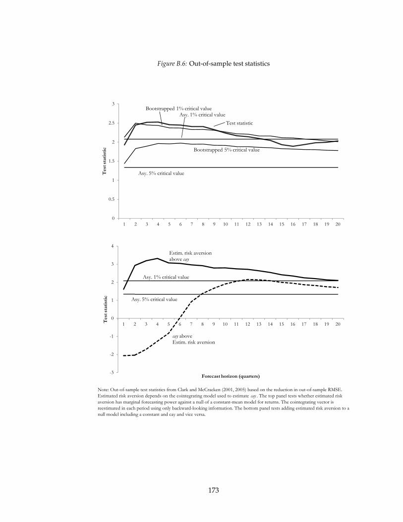
Figure B.6: Out-of-sample test statistics

Note: Out-of-sample test statistics from Clark and McCracken (2001, 2005) based on the reduction in out-of-sample RMSE.

Estimated risk aversion depends on the cointegrating model used to estimate cay . The top panel tests whether estimated risk

aversion has marginal forecasting power against a null of a constant-mean model for returns. The cointegrating vector is

reestimated in each period using only backward-looking information. The bottom panel tests adding estimated risk aversion to a

null model including a constant and cay and vice versa.

0

0.5

1

1.5

2

2.5

3

1 2 3 4 5 6 7 8 9 10 11 12 13 14 15 16 17 18 19 20

Test statistic

Asy. 1% critical value

Asy. 5% critical value

Test statistic

Bootstrapped 5% critical value

Bootstrapped 1% critical value

-3

-2

-1

0

1

2

3

4

1 2 3 4 5 6 7 8 9 10 11 12 13 14 15 16 17 18 19 20

Test statistic

Forecast horizon (quarters)

Asy. 1% critical value

Asy. 5% critical value

Estim. risk aversionabove cay

cay above Estim. risk aversion

173

each horizon from 1 to 20 quarters. I bootstrap 10,000 samples of data. The top panel of

figure B.2 plots the 95th and 99th percentiles of the bootstrapped test statistics, and the

out-of-sample forecasting power is still significant at the 5 percent level.

B.4.3.2 α versus cay

We can also use the out-of-sample test to ask whether estimated risk aversion forecasts

stock returns better than cay. The null model is now one where stock returns depend on

a constant and the lagged value of cay, and the encompassing alternative adds the lagged

value of α. The bottom panel of figure A2 plots the test statistics. At every horizon, we can

reject the null that α does not improve the forecast using cay at the 5 percent level, and we

can reject the null at the 1 percent level at every horizon longer than 1 quarter.

Figure B.2 also plots the statistic for a test of whether cay has any marginal predictive

power above that of α. At horizons shorter than 8 quarters, we cannot reject the null

that it does not. At longer horizons, though, there is evidence that both variables contain

important information for forecasting stock returns.

174

C. APPENDIX TO CHAPTER 3

C.1 Results from the text

C.1.1 Price of a utility claim and the SDF

The utility claim pays UtU−1C,t as its dividend. We confirm that its cum-dividend price

is WU,t = V1−ρt B−1

t U−1C,t / (1− β) by simply inserting this guess into the Euler equation,

WU,t = UtU−1C,t + Et [WU,t+1Mt+1] (C.1)

V1−ρt B−1

t U−1C,t / (1− β) = UtU−1

C,t + Et

V1−ρt+1 B−1

t+1U−1C,t+1

(1− β)β

Bt+1

Bt

UC,t+1

UC,t

Vρ−αtt+1(

EtV1−αtt+1

) ρ−αt1−αt

(C.2)

V1−ρt = (1− β) BtUt + βEt

V1−ρt+1

Vρ−αtt+1(

EtV1−αtt+1

) ρ−αt1−αt

(C.3)

V1−ρt = (1− β) BtUt + βEt

[V1−αt

t+1

] 1−ρ1−αt (C.4)

The last line shows that the guess for the price of the utility claim was in fact correct, since

the Euler equation is guaranteed to hold.

175

Next, we consider the return on the utility claim. We have

RU,t+1 =V1−ρ

t+1 B−1t+1U−1

C,t+1/ (1− β)

V1−ρt B−1

t U−1C,t / (1− β)−UtU−1

C,t

(C.5)

=V1−ρ

t−1

V1−ρt − (1− β) BtUt

(Bt+1UC,t+1

BtUC,t

)−1

(C.6)

=V1−ρ

t+1

β(

EtV1−αtt+1

) 1−ρ1−α

(Bt+1UC,t+1

BtUC,t

)−1

(C.7)

V1−ρt+1(

EtV1−αtt+1

) 1−ρ1−αt

ρ−αt1−ρ

= Rρ−αt1−ρ

U,t+1βρ−αt1−ρ

(UC,t+1

UC,t

) ρ−αt1−ρ(

Bt+1

Bt

) ρ−αt1−ρ

(C.8)

Now substitute the return into the SDF:

Mt+1 = βBt+1

Bt

UC,t+1

UC,tR

ρ−αt1−ρ

U,t+1βρ−αt1−ρ

(UC,t+1

UC,t

) ρ−αt1−ρ(

Bt+1

Bt

) ρ−αt1−ρ

(C.9)

= β1−αt1−ρ

(UC,t+1Bt+1

UC,tBt

) 1−αt1−ρ

Rρ−αt1−ρ

U,t+1 (C.10)

This is the formula from the text.

C.1.2 First-order condition for wage setting

0 = E∗t∞

∑k=0

ξkw

[ψt+k

1 + θw

θw

(Wt+k (j)

Wt+k

)− 1+θwθw Nt+k

Wt+j (j)− λt+kNt+k (j)

](C.11)

= E∗t∞

∑k=0

ξkw

[(dVt

dNt+k (j)+

dVt

dCt+k

Wt+k (j)Pt

)(1 + θw)− θw

dVt

dCt+k

Wt+k (j)Pt

]Nt+k (j)

(C.12)

= E∗t∞

∑k=0

ξkw

[dVt

dNt+k (j)(1 + θw) +

dVt

dCt+k

Wt+k (j)Pt

]Nt+k (j) (C.13)

= E∗t∞

∑k=0

ξkw

dVt/dCt+k

dVt/dCt

[dVt/dNt+k (j)

dVt/dCt+k(1 + θw) +

Wt+k (j)Pt

]Nt+k (j) (C.14)

176

C.2 Approximation method

This section proceeds as follows. First, I fix notation for a general set of equilibrium

conditions. Next, I describe the specifics of how to solve for the model’s equilibrium dy-

namics. Third, I show that the essentially affine approximation method delivers bond-

pricing formulas in the essentially affine class of Duffee (2002).

C.2.1 Equilibrium conditions

Denote the vector of the variables in the model (including the exogenous processes) as

Xt. In addition to the various variables described above that track the state of the economy

and the shocks, Xt will include the price/dividend ratio of the utility portfolio, the return

on the utility portfolio, and the marginal utility of consumption. The vector of fundamen-

tal shocks in the model is denoted εt ≡[εmp,t, εz,t, εb,t, εµ,t, εg,t, εp,t, εw,t, εα,t, επ∗,t

].

The equations determining the equilibrium of the model take the form

0 = G (Xt, Xt+1, σεt+1) (C.15)

where the expectation operator may appear in the function G.There is one equation for

each variable in the model. The new parameter σ is the usual parameter used in perturba-

tion approximations that controls the variance of the shocks. In the true model, σ = 1, but

we will consider an approximation around the point σ = 0.

The equations G can be divided into two types: those that do not involve taking expec-

tations over the SDF and those that do.

G (Xt, Xt+1, εt+1) =

D (Xt, Xt+1, σεt+1)

Et [M (Xt, Xt+1, σεt+1) F (Xt, Xt+1, σεt+1)]

(C.16)

where D and F are vector-valued functions and M is the (scalar-valued) stochastic discount

factor. Note that this formulation does not actually restrict F. Specifically, suppose there

were a set of equilibrium conditions 1 = Eth (xt, xt+1, σεt+1), i.e. that do not involve the

SDF. We could simply say that F (xt, xt+1, σεt+1) ≡ h (xt, xt+1, σεt+1) /M (xt, xt+1, σεt+1).

177

Note, though, that in this model, all expectational equations involve the SDF.

For the equations that do not involve the SDF, I use standard perturbation methods

and simply take a log-linear approximation. We approximate D as

0 = log (D (exp (xt) , exp (xt+1) , σεt+1) + 1) (C.17)

0 ≈ d0 + dx xt + dx′ xt+1 + dεσεt+1 (C.18)

where the terms d0, dx, dx′ , and dε are coefficients from a Taylor-series approximation and

xt ≡ log Xt

xt ≡ log Xt − log X

C.2.2 Linearizing the Euler equations

I now show that if we log-linearize the function F, we can transform (3.40) into a linear

condition that can be solved alongside the remaining equations. Mt+1 will not even be

log-linear in the state variables, but we will be able to state the equilibrium conditions as a

set of linear expectational difference equations.

First, guess that the approximated equilibrium dynamics of the model take the form

xt+1 = C + Φxt + Ψσεt+1 (C.19)

where xt ≡ log (Xt)− log (X). We confirm in the end that the solution to the approximated

equilibrium conditions actually takes this form. Next, define the matrices ΓUC, Γb, and Γr

as matrices that select individual elements of xt such that

uC,t = ΓUC xt, bt = Γb xt, rU,t = Γr xt (C.20)

where lower-case letters with circumflexes denote log deviations from non-stochastic steady-

state values. That is, uC,t ≡ log UC,t − log UC, etc.For the sake of arithmetical convenience,

also define an auxiliary variable ζt ≡ 1−αt1−ρ .

178

C.2.2.1 The essentially affine SDF

U =

(Cη

t C1−ηt−1

)1−ρ

1− ρ+ Z1−ρ

t ϕ1(H − Nt)

αH(1−ρ)

1− ρ

UC = ηcη(1−ρ)−1t c(1−η)(1−ρ)

t−1 Zη(1−ρ)−1t Z(1−η)(1−ρ)

t−1

= ηcη(1−ρ)−1t c(1−η)(1−ρ)

t−1 Z−(1−η)(1−ρ)t Z(1−η)(1−ρ)

t−1 Z−ρt

The SDF is

Mt+1 = β1−αt1−ρ

(UC,t+1

UC,tBt

1− βBt+1

1− βBt

) 1−αt1−ρ

Rρ−αt1−ρ

U,t+1 (C.21)

Mt+1 is completely log-linear in the endogenous variables UC,t and RU,t+1, but it is not

log-linear in Bt and Bt+1. If not for these terms, we could use the exact formula for Mt+1 in

what follows. Since those terms are non-linear, I use the approximations,

log1− β exp (bt+1)

exp (−bt)− β≈ 1

1− βbt −

β

1− βbt+1 (C.22)

m(1)t+1 ≡ m + ζt

(∆uC,t+1 +

11− β

bt −β

1− βbt+1

)+ (ζt − 1) rU,t+1 (C.23)

m(1)t+1 is first-order accurate for mt+1, hence the superscript. In the continuous time limit,

this formula becomes exact.

The Euler equation for the return on the utility portfolio is

1 = Et exp(

ζt

(∆uC,t+1 +

11− β

bt −β

1− βbt+1

)+ ζtrU,t+1

)(C.24)

Taking logs of both sides and taking advantage of log-normality gives

0 = EtuC,t+1 − uC,t +1

1− βbt −

β

1− βEtbt+1 + EtrU,t+1

+12

ζtσ2(

ΓUC −β

1− βΓb + Γr

)ΨΨ′

(ΓUC −

β

1− βΓb + Γr

)′(C.25)

179

Moreover, this implies that the approximated SDF can be written as

m(1)t+1 = ζt

(ΓUC −

β

1− βΓb + Γr

)Ψσεt+1 − Γr (Φxt + Ψσεt+1)− r

− 12

ζ2t σ2

(ΓUC −

β

1− βΓb + Γr

)ΨΨ′

(ΓUC −

β

1− βΓb + Γr

)′(C.26)

which is the essentially affine form from the text. The reason that this form is useful is that

any time the SDF is essentially affine, we can obtain an exact expression for

Et exp (mt+1 + f0 + fxxt + fx′xt+1). It also means that we can price any asset whose payoffs

are linear in the endogenous variables, including real and nominal bonds.

C.2.2.2 Approximation to F

Next, we take a first-order Taylor approximation to log F such that log F (xt, xt+1, εt+1) ≈

f0 + fxxt + fx′xt+1, giving

1 = Et exp(

m(1)t+1 + fxxt + fx′xt+1

)(C.27)

Taking logs and evaluating the expectation yields

0 = −EtrU,t+1 + fxxt + fx′Etxt+1 +12

σ2 (−Γr + fx′)ΨΨ′ (−Γr + fx′)′

+ ζtσ2(

ΓUC −β

1− βΓb + Γr

)ΨΨ′ (−Γr + fx′)

′ (C.28)

(C.28) is the equation that we ultimately place into the system to be solved. It is completely

linear in both xt and ζt (equivalently, αt).

C.2.2.3 Solution

Since every equation in the system is now linear in the variables of the model, we

can solve the system for the parameters Φ and Ψ from (C.19). Specifically, we solve the

180

following system,

0 = −EtrU,t+1 + fxxt + fx′Etxt+1 +12

σ2 (−Γr + fx′)ΨΨ′ (−Γr + fx′)′

+ ζtσ2(

ΓUC −β

1− βΓb + Γr

)ΨΨ′ (−Γr + fx′)

′ (C.29)

0 = d0 + dxxt + dx′xt+1 + dεσεt+1 (C.30)

where σ = 1 in the stochastic equilibrium that we approximate. This system can be solved

using, for example, Sims’ (2001) Gensys algorithm.

The last wrinkle here is that we cannot simply insert (C.28) into the set of equations to

be solved since it involves the matrix Ψ, which is one of the unknown structures we are

solving for. I deal with this with a simple fixed-point iteration: I begin with the equations

that we obtain from perturbation,

0 = −ΓrEtxt+1 + fxxt + fx′Etxt+1

0 = d0 + dx xt + dx′ xt+1 + dεσεt+1

which will deliver an initial value of Ψ, denoted Ψ(1). We then use Ψ(1) to change the

equilibrium condition to take the form

0 = −ΓrΦxt − r + fxxt + fx′Φxt +12

σ2 (−Γr + fx′)Ψ(1)Ψ(1)′ (−Γr + fx′)′

+ ζtσ2(

ΓUC −β

1− βΓb + Γr

)Ψ(1)Ψ(1)′ (−Γr + fx′)

′ (C.31)

0 = d0 + dx xt + dx′ xt+1 + dεσεt+1 (C.32)

which delivers a value Ψ(2). Then simply iterate to convergence. I treat parameter sets for

which the iteration diverges as inadmissible, setting the marginal likelihood to zero.

181

C.2.3 Bond pricing

To solve for bond prices, we guess that bond prices are log-linear in the vector of state

variables, so that

pn,t = An + Bnxt (C.33)

where pn,t is the price of a zero-coupon bond that matures on date t + n and pays 1 unit of

consumption. We can also write the price of a nominal bond as p$n,t. Using the formula for

the SDF from above, we have

exp(

p$n,t

)= Et exp

ζt

(ΓUC − β

1−β Γb + Γr

)Ψεt+1 − Γr (Φxt + Ψεt+1)− r

+An−1 + (Bn−1 − Γπ) (Φxt + Ψεt+1)

− 12 ζ2

t σ2(

ΓUC − β1−β Γb + Γr

)ΨΨ′ (ΓUC + Γb + Γr)

′

(C.34)

= −r− ΓrΦxt + An−1 + (Bn−1 − Γπ)Φxt

+12

σ2 (Bn−1 − Γπ − Γr)ΨΨ′ (Bn−1 − Γπ − Γr)′ (C.35)

+ σ2(

ΓUC −β

1− βΓb + Γr

)ΨΨ′ (Bn−1 − Γπ − Γr)

′ Γζ xt (C.36)

Matching coefficients gives

An = −r + An−1 +12

σ2 (Bn−1 − Γπ − Γr)ΨΨ′ (Bn−1 − Γπ − Γr)′ (C.37)

Bn = −ΓrΦ + (Bn−1 − Γπ)Φ +

(ΓUC −

β

1− βΓb + Γr

)ΨΨ′ (Bn−1 − Γπ − Γr)

′ Γζ (C.38)

C.3 Estimation

Much of the analysis discusses the behavior of the model around the posterior mode

(i.e. the peak of the posterior distribution; it is also a maximum-likelihood estimate penal-

ized by the prior distribution). I also start the Metropolis–Hastings chain from that point.

To search for the posterior mode, I begin by running a genetic algorithm on a population of

60 points drawn from the prior distribution. The genetic algorithm searches the parameter

space by mixing parameter sets in the population and also allowing random mutations.

After 30 iterations of the genetic algorithm, I take the point in the population with the

182

highest posterior density and use it as the starting point for Chris Sims’ CSMINWEL al-

gorithm, which is a derivative-based hill-climbing algorithm that is designed for DSGE

models. When CSMINWEL gets stuck, I also try the standard simplex algorithm.

I ran this combined search 2500 times (each search takes roughly an hour, so access to

a large computing cluster was essential). The point that I am calling the posterior mode

was found to be the peak in fewer than 100 of the searches. In other words, it is extremely

difficult to find the peak of the posterior likelihood. In general, I found that it was far

easier to find the posterior mode when risk aversion or the inflation target was held fixed,

and easier still when bond prices were also dropped from the estimation. Even though

the priors help to add curvature to the posterior likelihood surface, I still find many local

maxima, a problem that plagues the bond-pricing literature. Furthermore, since the model

is so highly constrained there is no straightforward way to use the more recent estimation

algorithms for affine term structure models proposed by, for example, Hamilton and Wu

(2012) and Joslin, Singleton, and Zhu (2010).

I simulate the posterior distribution using the adaptive random-walk Metropolis–

Hastings algorithm of Haario, Saksman, and Tamminen (2001). I initialize the chain at the

posterior mode. For the proposal distribution, I begin with a normal distribution whose

variance matrix is equal to that of the prior, multiplied by (2.382)/d, where d is the dimen-

sion of the parameter vector (49), which is the optimal scaling factor of Gelman, Roberts,

and Gilks (1996). After 10,000 iterations of the algorithm, I update the variance matrix of

the proposal distribution to be equal to the observed variance matrix for the first 10,000

iterations of the chain. Subsequently, the variance is updated each on each iteration using

the sample variance of the chain up to the current iteration.1 I achieve relatively rapid

mixing this way. The full chain has 1,000,000 draws, but it mixes well even by 100,000

draws.

1 A more common method in the DSGE literature is to use the hessian of the posterior around the posteriormode to determine the variance of the proposal distribution. I have difficulty calculating the hessian due tonumerical instability.

183

BIBLIOGRAPHY

ABEL, A. B. (1990): “Asset Prices under Habit Formation and Catching up with the Jone-

ses,” The American Economic Review, Papers and Proceedings, 80(2), 38–42.

(1999): “Risk Premia and Term Premia in General Equilibrium,” Journal of Monetary

Economics, 43(1), 3–33.

ABEL, A. B., AND O. J. BLANCHARD (1986): “The Present Value of Profits and Cyclical

Movements in Investment,” Econometrica, 54(2), 249–273.

ABEL, A. B., A. K. DIXIT, J. C. EBERLY, AND R. S. PINDYCK (1996): “Options, the Value of

Capital, and Investment,” Quarterly Journal of Economics, 111(3), 753–777.

ALVAREZ, F., AND U. J. JERMANN (2005): “Using Asset Prices to Measure the Persistence

of the Marginal Utility of Wealth,” Econometrica, 73(6), 1977–2016.

ANDREWS, D. W. (1993): “Tests for Parameter Instability and Structural Change with Un-

known Change Point,” Econometrica, 61(4), 821–856.

ANG, A., AND M. PIAZZESI (2003): “No-Arbitrage Vector Autoregression of Term Struc-

ture Dynamics with Macroeconomic and Latent Variables,” Journal of Monetary Eco-

nomics, 50, 745–787.

ATKESON, A., AND L. E. OHANIAN (2001): “Are Phillips Curves Useful for Forecasting

Inflation?,” Federal Reserve Bank of Minneapolis Quarterly Review, 25(1), 2–11.

ATTANASIO, O. P., P. K. GOLDBERG, AND E. KYRIAZIDOU (2008): “Credit Constraints in

the Market for Consumer Durables: Evidence from Micro Data on Car Loans,” Interna-

tional Economic Review, 49(2), 401–436.

184

BAKER, M., R. GREENWOOD, AND J. WURGLER (2003): “The Maturity of Debt Issues and

Predictable Variation in Bond Returns,” Journal of Financial Economics, 70(2), 261–291.

BANSAL, R., AND A. YARON (2004): “Risks for the Long Run: A Potential Resolution of

Asset Pricing Puzzles,” Journal of Finance, 59(4), 1481–1509.

BARBERIS, N., M. HUANG, AND T. SANTOS (2001): “Prospect Theory and Asset Prices,”

Quarterly Journal of Economics, 116(1), 1–53.

BARCLAY, M. J., AND J. CLIFFORD W. SMITH (1995): “The Maturity Structure of Corporate

Debt,” Journal of Finance, 50(2), 609–631.

BASU, S., J. G. FERNALD, AND M. S. KIMBALL (2006): “Are Technology Improvements

Contractionary?,” American Economic Review, 96(5), 1418–1448.

BAXTER, M., AND M. J. CRUCINI (1993): “Explaining Saving–Investment Correlations,”

American Economic Review, 83(3), 416–436.

BEELER, J., AND J. Y. CAMPBELL (2011): “The Long-Run Risks Model and Aggregate Asset

Prices: An Empirical Assessment,” Working paper.

BEKAERT, G., S. CHO, AND A. MORENO (2010): “new Keynesian Macroeconomics and the

Term Structure,” Journal of Money, Credit ans Banking, 42(1), 33–62.

BERK, J. B., R. C. GREEN, AND V. NAIK (1999): “Optimal Investment, Growth Options,

and Security Returns,” Journal of Finance, 54(5), 1553–1607.

BERNANKE, B. S., AND M. GERTLER (1995): “Inside the Black Box: The Credit Channel of

Monetary Policy Transmission,” Journal of Economic Perspectives, 9(4), 27–48.

BEVERIDGE, S., AND C. R. NELSON (1981): “A New Approach to Decomposition of Eco-

nomic Time Series into Permanent and Transitory Components with Particular Attention

to Measurement of the "Business Cycle",” Journal of Monetary Economics, 7(2), 151–174.

BLOOM, N. (2009): “The Impact of Uncertainty Shocks,” Econometrica, 77(3), 623–685.

BOLDRIN, M., L. J. CHRISTIANO, AND J. D. M. FISHER (2001): “Habit Persistence, Asset

Returns, and the Business Cycle,” American Economic Review, 91(1), 149–166.

185

BRUNNERMEIER, M., AND S. NAGEL (2008): “Do Wealth Fluctuations Generate Time-

Varying Risk Aversion? Micro-Evidence on Individuals’ Asset Allocation,” The American

Economic Review, 98(3), 713–736.

CABALLERO, R. J. (1994): “Small Sample Bias and Adjustment Costs,” Review of Economics

and Statistics, 76(1), 52–58.

CALDARA, D., J. FERNANDEZ-VILLAVERDE, J. F. RUBIO-RAMIREZ, AND Y. WEN (2009):

“Computing DSGE Models with Recursive Preferences,” Working paper.

CALVET, L. E., J. Y. CAMPBELL, AND P. SODINI (2009): “Fight Or Flight? Portfolio Rebal-

ancing by Individual Investors,” The Quarterly Journal of Economics, 124(1), 301–348.

CALVET, L. E., AND P. SODINI (2010): “Twin Picks: Disentangling the Determinants of

Risk-Taking in Household Portfolios,” Working Paper.

CAMPANALE, C., R. CASTRO, AND G. L. CLEMENTI (2010): “Asset Pricing in a Production

Economy with Chew-Dekel Preferences,” Review of Economic Dynamics, 13(2), 379–402.

CAMPBELL, J. Y. (1987): “Stock Returns and the Term Structure,” Journal of Financial Eco-

nomics, 18(2), 373–399.

(1994): “Inspecting the Mechanism: An Analytical Approach to the Stochastic

Growth Model,” Journal of Monetary Economics, 33(3), 463–506.

(2003): “Consumption-Based Asset Pricing,” in Handbook of the Economics of Finance,

vol. 1, pp. 803–887. Elsevier Science.

CAMPBELL, J. Y., AND J. H. COCHRANE (1999): “By Force of Habit: A Consumption-Based

Explanation of Aggregate Stock Market Behavior,” Journal of Political Economy, 107(2),

205–251.

CAMPBELL, J. Y., AND A. DEATON (1989): “Why is Consumption so Smooth?,” Review of

Economic Studies, 56(3), 357–373.

186

CAMPBELL, J. Y., M. LETTAU, B. G. MALKIEL, AND Y. XU (2001): “Have Individual Stocks

Become More Volatile? an Empirical Exploration of Idiosyncratic Risk,” Journal of Fi-

nance, 56(1), 1–43.

CAMPBELL, J. Y., AND N. G. MANKIW (1989): “Consumption, Income and Interest Rates:

Reinterpreting the Time Series Evidence,” in NBER Macroeconomics Annual, ed. by O. J.

Blanchard, and S. Fischer.

CAMPBELL, J. Y., AND R. J. SHILLER (1988): “The Dividend-Price Ratio and Expectations

of Future Dividends and Discount Factors,” Review of Financial Studies, 1(3)(3), 195–228.

(1991): “Yield Spreads and Interest Rate Movements: A Bird’s Eye View,” Review

of Economic Studies, 58(3), 495–514.

CARROLL, C. D. (2002): “Portfolios of the Rich,” in Household Portfolios, ed. by L. Guiso,

M. Haliassos, and T. Japelli. MIT Press.

CHIRINKO, R. S. (1993): “Business Fixed Investment Spending: Modeling Strategies, Em-

pirical Results, and Policy Implications,” Journal of Economic Literature, 31(4), 1875–1911.

CHRISTIANO, L. J., M. EICHENBAUM, AND R. VIGFUSBSON (2004): “The Response of

Hours to a Technology Shock: Evidence Based on Direct Measures of Technology,” Jour-

nal of the European Economic Association, 2(2–3), 381–395.

CHRISTIANO, L. J., M. TRABANDT, AND K. WALENTIN (2011): “DSGE Models for Mone-

tary Policy Analysi,” in Handbook of Monetary Economics. North-Holland.

CLARK, T. E., AND M. W. MCCRACKEN (2001): “"Tests of Equal Forecast Accuracy and

Encompassing for Nested Models",” Journal of Econometrics, 105(1), 85–110.

(2005): “Evaluating Direct Multistep Forecasts,” Econometric Reviews, 24(4), 369–

404.

CLARK, T. E., AND K. D. WEST (2007): “Approximately Normal Tests for Equal Predictive

Accuracy in Nested Models,” Journal of Econometrics, 138(1), 291–311.

187

COCHRANE, J. H. (1991): “Production-Based Asset Pricing and the Link Between Stock

Returns and Economic Fluctuations,” Journal of Finance, 46(1), 209–237.

(1996): “A Cross-Sectional Test of an Investment-Based Asset Pricing Model,” Jour-

nal of Political Economy, 104(3), 572–621.

(2005): “Financial Markets and the Real Economy,” NBER Working paper.

(2008): “The Dog That Did Not Bark: A Defense of Return Predictability,” Review

of Financial Studies, 21(4), 1533–1575.

(2011): “Discount Rates,” Journal of Finance, 66(4), 1047–1108, AFA Presidential

Address.

COCHRANE, J. H., AND M. PIAZZESI (2005): “Bond Risk Premia,” American Economic Re-

view, 95(1), 138–160.

CONSTANTINIDES, G. M. (1990): “Habit Formation: A Resolution of the Equity Premium

Puzzle,” The Journal of Political Economy, 98(3), 519–543.

DANTHINE, J.-P., J. B. DONALDSON, AND R. MEHRA (1992): “The Equity Premium and

the Allocation of Income Risk,” Journal of Economic Dynamics and Control, 16(3–4), 509–

532.

DEW-BECKER, I. (2011a): “Bond Pricing With a Time-varying Price Of Risk in an Estimated

Medium-Scale Bayesian DSGE Model,” Working paper.

(2011b): “A Model of Time-Varying Risk Premia with Habits and Production,”

Working paper.

(2012): “Essentially affine approximations for economic models,” Working paper.

DOH, T. (2011): “Yield Curve in an Estimated Nonlinear Macro Model,” Journal of Economic

Dynamics & Control.

DUFFEE, G. R. (2002): “Term Premia and Interest Rate Forecasts in Affine Models,” Journal

of Finance, 57(1), 405–443.

188

DYNAN, K. E. (1993): “How Prudent are Consumers?,” Journal of Political Economy, 101(6),

1104–1113.

(2000): “Habit Formation in Consumer Preferences: Evidence from Panel Data,”

American Economic Review, 90(3), 391–406.

EBERLY, J., S. REBELO, AND N. VINCENT (2009): “Investment and Value: A Neoclassical

Benchmark,” NBER Working Paper.

EDGE, R. M. (2000): “The Effect of Monetary Policy on Residential and Structures In-

vestment Under Differential Project Planning and Completion Times,” Federal Reserve

Board of Governors International Finance Discussion Papers No. 671.

EPSTEIN, L. G., AND S. E. ZIN (1989): “Substitution, Risk Aversion, and the Temporal

Behavior of Consumption and Asset Returns: A Theoretical Framework,” Econometrica,

57(4), 937–969.

(1991): “Substitution, Risk Aversion, and the Temporal Behavior of Consumption

and Asset Returns: An Empirical Analysis,” The Journal of Political Economy, 99(2), 263–

286.

FAMA, E. F., AND K. R. FRENCH (1989): “Business Conditions and Expected Returns on

Stocks and Bonds,” Journal of Financial Economics, 25(1), 23–49.

FAMA, E. F., AND G. W. SCHWERT (1977): “Human Capital and Capital Market Equilib-

rium,” Journal of Financial Economics, 4(1), 95–125.

FAZZARI, S. M., R. G. HUBBARD, AND B. C. PETERSEN (1988): “Financing Constraints and

Corporate Investment,” Brookings Papers on Economic Activity, 1988(1), 141–206.

FERNANDEZ-VILLAVERDE, J., P. GUERRON, J. F. RUBIO-RAMIREZ, AND M. URIBE (2011):

“Risk Matters: The Real Effects of Volatility Shocks,” American Economic Review.

FERNANDEZ-VILLAVERDE, J., AND J. RUBIO-RAMIREZ (2004): “Comparing dynamic equi-

librium models to data: a Bayesian approach,” Journal of Econometrics, 123(1), 153–187.

189

FRANCIS, N., AND V. A. RAMEY (2005): “Is the Technology-Driven Real Business Cycle

Hypothesis Dead? Shocks and Aggregate Fluctuations Revisited,” Journal of Monetary

Economics, 52(8), 1379–1399.

(2009): “Measures of Per Capita Hours and Their Implications for the Technology-

Hours Debate,” Journal of Money, Credit, and Banking, 41(6), 1071–1097.

FRAUMENI, B. (1997): “The Measurement of Depreciation in the U.S. National Income and

Product Accounts,” Survey of Current Business, pp. 7–23.

GALI, J. (1999): “Technology, Employment, and the Business Cycle: Do Technology Shocks

Explain Aggregate Fluctuations?,” American Economic Review, 89(1), 249–271.

GELFAND, A. E., AND D. K. DEY (1994): “Bayesian Model Choice: Asymptotics and Exact

Calculations,” Journal of the Royal Statistical Society. Series B, 56(3), 501–514.

GELMAN, A., G. ROBERTS, AND W. GILKS (1996): “Efficient Metropolis Jumping Rules,”

in Bayesian Statistics, ed. by J. Bernardo, J. Berger, A. Dawid, and A. Smith, vol. 5. Oxford

University Press.

GERTNER, R. (1993): “Game Shows and Economic Behavior: Risk-Taking on "Card

Sharks",” Quarterly Journal of Economics, 108(2), 507–521.

GEWEKE, J. (1999): “Using simulation methods for bayesian econometric models: infer-

ence, development,and communication,” Econometric Reviews, 18(1), 1–73.

GILCHRIST, S., AND E. ZAKRAJSEK (2007): “Investment and the Cost of Capital: New

Evidence from the Corporate Bond Market,” Working Paper.

GOMES, J. F., L. KOGAN, AND M. YOGO (2009): “Durability of Output and Expected Stock

Returns,” Journal of Political Economy, 117(5), 941–986.

GOURIO, F. (2010): “Disaster Risk and Business Cycles,” Working Paper.

GRAEVE, F. D., M. DOSSCHE, M. EMIRIS, H. SNEESSENS, AND R. WOUTERS (2010): “Risk

premiums and macroeconomic dynamics in a heterogeneous agent model,” Journal of

Economic Dynamics and Control, 34(9), 1680–1699.

190

GRAHAM, J. R., AND C. R. HARVEY (2002): “How do CFOs Make Capital Budgeting and

Capital Structure Decisions?,” Journal of Applied Corporate Finance, 15(1), 8–23.

GREENWOOD, R., S. HANSON, AND J. STEIN (2009): “A Gap-Filling Theory of Corporate

Debt Maturity Choice,” Working Paper.

GROSSMAN, S. J., AND R. J. SHILLER (1981): “The Determinants of the Variability of Stock

Market Prices,” American Economic Review, Papers and Proceedings, 71(2), 222–227.

GRUBER, J. (2006): “A Tax-Based Estimate of the Elasticity of Intertemporal Substitution,”

NBER Working Paper 11945.

GUEDES, J., AND T. OPLER (1996): “The Determinants of the Maturity of Corporate Debt

Issues,” The Journal of Finance, 51(5), 1809–1833.

GUISO, L., A. K. KASHYAP, F. PANETTA, AND D. TERLIZZESE (2002): “How Interest Sen-

sitive is Investment? Very (when the data are well measured),” Working Paper.

GUISO, L., P. SAPIENZA, AND L. ZINGALES (2011): “Time-Varying Risk Aversion,” .

GURKAYNAK, R. S., B. SACK, AND E. SWANSON (2005): “The Sensitivity of Long-Term In-

terest Rates to Economic News: Evidence and Implications for Macroeconomic Models,”

American Economic Review, 95(1), 425–436.

GUVENEN, F. (2009): “A Parsimonious Macroeconomic Model for Asset Pricing,” Econo-

metrica, 77(6), 1711–1750.

HAARIO, H., E. SAKSMAN, AND J. TAMMINEN (2001): “An Adaptive Metropolis Algo-

rithm,” Bernoulli, 7(2), 223–242.

HALL, R. E. (1988): “Intertemporal Substitution in Consumption,” Journal of Political Econ-

omy, 96(2), 339–357.

HAMILTON, J. D., AND C. WU (2012): “Identification and Estimation of Gaussian Affine-

Term-Structure Models,” Journal of Econometrics, Working Paper.

HANSEN, L. P., J. C. HEATON, AND N. LI (2008): “Consumption Strikes Back? Measuring

Long-Run Risk,” Journal of Political Economy, 116(2), 260–302.

191

HANSEN, L. P., AND R. JAGANNATHAN (1991): “Implications of Security Market Data for

Models of Dynamic Economies,” Journal of Political Economy, 99(2), 225–262.

HASSETT, K. A., AND R. G. HUBBARD (2002): Handbook of Public Economicschap. Tax Policy

and Business Investment, pp. 1293–1343. Elsevier Science B.V.

HOUSE, C. L., AND M. D. SHAPIRO (2008): “Temporary Investment Tax Incentives: Theory

with Evidence from Bonus Depreciation,” American Economic Review, 98(3), 737–768.

HULTEN, C. R., AND F. C. WYKOFF (1981): “The Measurement of Economic Depreciation,”

in Depreciation, Inflation, and the Taxation of Income from Capital,, ed. by C. R. Hulten, pp.

81–125. The Urban Institute Press, Washington, D.C.

JACCARD, I. (2007): “Asset Returns and Labor Supply in a Production Economy With

Habit Memory,” ECB Working Paper.

JERMANN, U. J. (1998): “Asset Pricing in Production Economies,” Journal of Monetary Eco-

nomics, 41(2), 257–275.

JOSLIN, S., K. J. SINGLETON, AND H. ZHU (2011): “A New Perspective on Gaussian Dy-

namic Term Structure Models,” Review of Financial Studies, 24(3), 926–970.

JUDD, K. L. (1999): Numerical Methods for Economists. MIT Press, Cambridge, MA.

JUSTINIANO, A., G. PRIMICERI, AND A. TAMBALOTTI (2010): “Investment Shocks and

Business Cycles,” Journal of Monetary Economics, 57(2), 132–145.

KALTENBRUNNER, G., AND L. A. LOCHSTOER (Forthcoming): “Long-Run Risk Through

Consumption Smoothing,” The Review of Financial Studies.

KASHYAP, A. K., AND J. C. STEIN (2000): “What Do a Million Observations on Banks Say

About the Transmission of Monetary Policy?,” American Economic Review, 90(3), 407–428.

KIEFER, N. M., AND T. J. VOGELSANG (2005): “A New Asymptotic Theory for

Heteroskedasticity-Autocorrelation Robust Tests,” Econometric Theory, 21(6), 1130–1164.

KIEFER, N. M., T. J. VOGELSANG, AND H. BUNZEL (2000): “Simple Robust Testing of

Regression Hypotheses,” Econometrica, 68(3), 695–714.

192

KING, R. G., C. I. PLOSSER, AND S. T. REBELO (1988): “Production, Growth and Business

Cycles : I. The Basic Neoclassical Model,” Journal of Monetary Economics, 21(2–3), 195–

232.

KREPS, D. M., AND E. L. PORTEUS (1978): “Temporal Resolution of Uncertainty and Dy-

namic Choice Theory,” Econometrica, 46(1), 185–200.

LEROY, S. F., AND R. D. PORTER (1981): “The Present-Value Relation: Tests Based on

Implied Variance Bounds,” Econometrica, 49(3), 555–574.

LETTAU, M. (2003): “Inspecting The Mechanism: Closed-Form Solutions for Asset Prices

in Real Business Cycle Model,” The Economic Journal, 113(489), 550–575.

LETTAU, M., AND S. LUDVIGSON (2001): “Consumption, Aggregate Wealth, and Expected

Stock Returns,” Journal of Finance, 56(3), 815–849.

LETTAU, M., AND H. UHLIG (2000): “Can Habit Formation be Reconciled with Business

Cycle Facts?,” Review of Economic Dynamics, 3(1), 79–99.

LETTAU, M., AND J. A. WACHTER (2007): “Why Is Long-Horizon Equity Less Risky? A

Duration-Based Explanation of the Value Premium,” Journal of Finance, 62(1), 55–92.

LONGSTAFF, F. A., AND E. S. SCHWARTZ (1992): “Interest Rate Volatility and the Term

Structure: A Two-Factor General Equilbrium Model,” Journal of Finance, 47(4), 1259–

1282.

LOWN, C. S., AND D. P. MORGAN (2006): “The Credit Cycle and the Business Cycle: New

Findings Using the Loan Officer Opinion Survey,” Journal of Money, Credit, and Banking,

38(6), 1575–1597.

MELINO, A., AND A. X. YANG (2003): “State-Dependent Preferences can Explain the Eq-

uity Premium Puzzle,” Review of Economic Dynamics, 6(4), 806–830.

MIAO, J., AND P. WANG (2010): “Credit Risk and Business Cycles,” Working Paper.

193

OLINER, S. D., G. D. RUDEBUSCH, AND D. SICHEL (1995): “New and Old Models of Busi-

ness Investment: A Comparison of Forecasting Performance,” Journal of Money, Credit,

and Banking, 27(3), 806–826.

(1996): “The Lucas Critique Revisited: Assessing the Stability of Empirical Euler

Equations for Investment,” Journal of Econometrics, 70(1), 291–316.

OPLER, T., L. PINKOWITZ, R. STULZ, AND R. WILLIAMSON (1999): “The Determinants

and Implications of Corporate Cash Holding,” Journal of Financial Economics, 52(1), 3–46.

PIAZZESI, M. (2010): “Affine Term Structure Models,” in Handbook of Financial Economet-

rics. Elsevier.

POST, T., M. J. VAN DEN ASSEM, G. BALTUSSEN, AND R. H. THALER (2008): “Deal or No

Deal? Decision Making under Risk in a Large-Payoff Game Show,” American Economic

Review, 98(1), 38–71.

RAVINA, E. (2007): “Habit Formation and Keeping Up with the Joneses: Evidence from

Micro Data,” Mimeo.

ROUWENHORST, K. G. (1995): “Asset Pricing Implications of Equilibrium Business Cycle

Models,” in Frontiers of Business Cycle Research, ed. by T. F. Cooley, chap. 10, pp. 294–330.

Princeton University Press.

RUDEBUSCH, G. D., AND E. T. SWANSON (2008): “Examining the Bond Premium Puzzle

with a DSGE Model,” Journal of Monetary Economics, 55(Supplement 1), S111–S126.

(Forthcoming): “The Bond Premium in a DSGE Model with Long-Run Real and

Nominal Risks,” American Economic Journal: Macroeconomics, Federal Reserve Bank of

San Francisco Working Paper 2008-31.

SCHALLER, H. (2006): “Estimating the Long-Run User Cost Elasticity,” Journal of Monetary

Economics, 53(4), 725–736.

SHILLER, R. J. (1981): “Do Stock Prices Move Too Much to be Justified by Subsequent

Changes in Dividends?,” American Economic Review, 71(3), 421–436.

194

SOLOW, R. M. (1957): “Technical Change and the Aggregate Production Function,” Review

of Economics and Statistics, 39(3), 312–320.

STOHS, M. H., AND D. C. MAUER (1996): “The Determinants of Corporate Debt Maturity

Structure,” The Journal of Business, 69(3), 279–312.

SUMMERS, L. H. (1981): “Taxation and Corporate Investment: A q-Theory Approach,”

Brookings Papers on Economic Activity, 1981(1), 67–140.

SWANSON, E. T. (2011): “Risk Aversion and the Labor Margin in Dynamic Equilibrium

Models,” American Economic Review.

TALLARINI, T. D. (2000): “Risk-Sensitive Real Business Cycles,” Journal of Monetary Eco-

nomics, 45(3), 507–532.

TANAKA, T., C. F. CAMERER, AND Q. NGUYEN (2010): “Risk and Time Preferences: Link-

ing Experimental and Household Survey Data from Vietnam,” American Economic Re-

view, 100(1), 557–571.

TEVLIN, S., AND K. WHELAN (2003): “Explaining the Investment Boom of the 1990s,”

Journal of Money, Credit, and Banking, 35(1), 1–22.

TITMAN, S., AND R. WESSELS (1988): “The Determinants of Capital Structure Choice,”

Journal of Finance, 43(1), 1–19.

VAN ARK, B., AND R. INKLAAR (2006): “Catching up or getting stuck? Europe’s troubles

to exploit ICT’s productivity potential,” GGDC Research Memorandum GD-79.

VAN BINSBERGEN, J. H., J. FERNANDEZ-VILLAVERDE, R. S. KOIJEN, AND J. F. RUBIO-

RAMIREZ (2011): “The Term Structure of Interest Rates in a DSGE Model with Recursive

Preferences,” Working paper.

VISSING-JORGENSEN, A., AND O. P. ATTANASIO (2003): “Stock-Market Participation, In-

tertemporal Substitution, and Risk-Aversion,” The American Economic Review, 93(2), 383–

391.

195

VISSING-JORGENSON, A. (2002): “Limited Asset Market Participation and the Elasticity of

Intertemporal Substitution,” Journal of Political Economy, 110(4), 825–853.

WACHTER, J. A. (2010): “Can Time-Varying Risk of Rare Disasters Explain Aggregate

Stock Market Volatility?,” Working Paper.

WEIL, P. (1989): “The Equity Premium Puzzle and the Risk-Free Rate Puzzle,” Journal of

Monetary Economics, 24(3), 401–421.

WOODFORD, M. (2003): Interest and Prices. Princeton University Press, Princeton, NJ.

YANG, W. (2008): “Intertemporal Substitution and Equity Premium: A Perspective With

Habit in Epstein-Zin Preferences,” Working Paper.

196