University of Kentucky University of Kentucky

UKnowledge UKnowledge

Theses and Dissertations--Agricultural Economics Agricultural Economics

2014

ESSAYS ON THE VALUE OF A FIRM’S ECO-FRIENDLINESS IN THE ESSAYS ON THE VALUE OF A FIRM’S ECO-FRIENDLINESS IN THE

FINANCIAL ASSET MARKET FINANCIAL ASSET MARKET

Muhammad S. Ahmadin University of Kentucky, msahma1@g.uky.edu

Right click to open a feedback form in a new tab to let us know how this document benefits you. Right click to open a feedback form in a new tab to let us know how this document benefits you.

Recommended Citation Recommended Citation Ahmadin, Muhammad S., "ESSAYS ON THE VALUE OF A FIRM’S ECO-FRIENDLINESS IN THE FINANCIAL ASSET MARKET" (2014). Theses and Dissertations--Agricultural Economics. 31. https://uknowledge.uky.edu/agecon_etds/31

This Doctoral Dissertation is brought to you for free and open access by the Agricultural Economics at UKnowledge. It has been accepted for inclusion in Theses and Dissertations--Agricultural Economics by an authorized administrator of UKnowledge. For more information, please contact UKnowledge@lsv.uky.edu.

STUDENT AGREEMENT: STUDENT AGREEMENT:

I represent that my thesis or dissertation and abstract are my original work. Proper attribution

has been given to all outside sources. I understand that I am solely responsible for obtaining

any needed copyright permissions. I have obtained needed written permission statement(s)

from the owner(s) of each third-party copyrighted matter to be included in my work, allowing

electronic distribution (if such use is not permitted by the fair use doctrine) which will be

submitted to UKnowledge as Additional File.

I hereby grant to The University of Kentucky and its agents the irrevocable, non-exclusive, and

royalty-free license to archive and make accessible my work in whole or in part in all forms of

media, now or hereafter known. I agree that the document mentioned above may be made

available immediately for worldwide access unless an embargo applies.

I retain all other ownership rights to the copyright of my work. I also retain the right to use in

future works (such as articles or books) all or part of my work. I understand that I am free to

register the copyright to my work.

REVIEW, APPROVAL AND ACCEPTANCE REVIEW, APPROVAL AND ACCEPTANCE

The document mentioned above has been reviewed and accepted by the student’s advisor, on

behalf of the advisory committee, and by the Director of Graduate Studies (DGS), on behalf of

the program; we verify that this is the final, approved version of the student’s thesis including all

changes required by the advisory committee. The undersigned agree to abide by the statements

above.

Muhammad S. Ahmadin, Student

Dr. Michael Reed, Major Professor

Dr. Michael Reed, Director of Graduate Studies

ESSAYS ON THE VALUE OF A FIRM’S ECO-FRIENDLINESS

IN THE FINANCIAL ASSET MARKET

_____________________________

Dissertation

_____________________________

A dissertation submitted in partial fulfillment of the

requirements for the degree of Doctor of Philosophy in the

College of Agriculture, Food, and Environment

At the University of Kentucky

By:

Muhammad S Ahmadin, BBA, MBA, MS

Director: Dr. Michael Reed

Co-Director: Dr. John K. Schieffer

Lexington, Kentucky

Copyright © 2014 Muhammad S. Ahmadin

ABSTRACT OF DISSERTATION

ESSAYS ON THE VALUE OF A FIRM’S ECO-FRIENDLINESS

IN THE FINANCIAL ASSET MARKET

This dissertation presents three different closely related topics on the value of eco-

friendliness in the financial market. The first essay attempts to estimate hedonic stock price

model to find a contemporaneous relationship between stock return and firms’

environmental performance and recover the value of investor’s willingness to pay of eco-

friendliness. This study follows stock and environmental performances of the 500 largest

US firms from 2009 to 2012. The firms’ environmental data come from the Newsweek

Green Ranking, both aggregate measures: green ranking (GR) and green score (GS), and

disaggregate measures: environmental impact score (EIS), green policy and performance

score (GPS), reputation survey score (RSS), and environmental disclosure score (EDS).

The results show a non-linear relationship between environmental variables and stock

return, i.e. upside down bowl shape or increasing in decreasing rate. That means for low

green ranking firms the marginal effect is positive while for high green ranking firms the

marginal effect is negative. The investor’s willingness to pay (WTP) for a greener stock

for firms in the lowest 25 green ranking, on average, is 0.0096% higher stock price

The second essays attempt to determine if a firm’s environmental performance

affects future systematic risk. Systematic risk measures an individual stock’s volatility

relative to the market price. This study also uses the Newsweek Green Ranking’s

environmental variables. The results show significant evidence of a non-linear relationship

between green variables and systematic (market) risk, but the shape is not unanimous for

all environmental variables. The shape of the relationship for green ranking (GR), for

example, is U-shape. This means that for the firms in the bottom rank, improving rank will

lower systematic (market) risk, and for the firms in the top rank improving rank will

increase systematic (market) risk. On average the marginal effect for the firms in the

bottom and top 25 firms are -0.2% and 0.09% respectively.

The third essay is the effect of a firm’s environmental performances on a firm’s

idiosyncratic risk. Idiosyncratic risk measures an individual stock’s volatility independent

from the market price. This study also uses the Newsweek Green Ranking’s environmental

variables. The results show significant non-linear relationships between environmental

variables and idiosyncratic risk, even though there is no unanimous shape among the

environmental variables. In the case of green ranking, for example, it has U-shape; for the

firms in the bottom rank, improving green ranking will lower idiosyncratic risk and for

firm in the top green ranking, improving green ranking will increase idiosyncratic risk. On

average the marginal effect for firm in bottom and top 25 firms are -0.4% and 0.2%

respectively.

KEYWORDS: Hedonic Stock Price Model, Newsweek Green Ranking,

CAPM, Systematic Risk, Idiosyncratic risk.

Muhammad S. Ahmadin

Student’s Signature

December 17, 2014

Date

ESSAYS ON THE VALUE OF A FIRM’S ECO-FRIENDLINESS

IN THE FINANCIAL ASSET MARKET

By: Muhammad S Ahmadin, BBA, MBA, MS

Dr. Michael Reed

Director of Dissertation

Dr. John K. Schieffer

Co-Director of Dissertation

Dr. Michael Reed

Director of Graduate Studies

Almarhum Bapakku

Ibukku

Istriku

Sedulur-sedulurku

Anak-anakku

iii

ACKNOWLEDGEMENT

I wish to express my sincere gratitude to my advisors Dr. Michael Reed (Chair)

and Dr. John Schieffer (Co-Chair), whose guidance, support, and patience throughout

this process made this dissertation possible. I also wish to acknowledge my

dissertation committee members, Dr. Wuyang Hu and Dr. Donald Mullineaux, for

their input and support. I also wish to acknowledge Dr. Jeffery Talbert for serving as

my dissertation external committee member.

Part of this studies, especially in the early concept, benefitted from the input

provided by participants of the 2011 Departmental Brown Bag Seminar at University

of Kentucky, and the 2011 Annual Meeting, the SAEA in Corpus Christi, TX. I also

indebted to the committee members in the Second Year paper: Dr. Michael Reed, Dr.

Wuyang Hu, and Dr. David Freshwater.

I am also fortunate to have encouragement and support from my late father

Mohamad Anwar (I wish you were here!), my mother Siti Masrowiyah, my lovely wife

Yeppy Hartuti, my awesome children: Saifu & Ayna, Irsyad, and Raiffa.

iv

Table of Content

ACKNOWLEDGEMENT ................................................................................................. iii

Table of Content ................................................................................................................ iv

List of Table ....................................................................................................................... vi

List of Figure..................................................................................................................... vii

List of Appendix .............................................................................................................. viii

Chapter 1: Introduction ....................................................................................................... 1

Chapter 2: A Hedonic Stock Price Model for Environmentally Friendly American Largest

Firms ................................................................................................................................... 4

1. Introduction ....................................................................................................................4

2. Literature Review...........................................................................................................6

2.1. Earlier Studies on Firms’ Eco-friendliness and Stock Return ................................6

2.2. The Hedonic Model for Stock Price: A Theoretical Framework .........................16

2.3. The Capital Assets Pricing Model (CAPM) .........................................................22

3. Methodology ................................................................................................................24

3.1. Empirical Model ...................................................................................................24

3.2. Data for the Study .................................................................................................25

3.3. Some Issues in the Model Estimation ..................................................................28

4. Results and Discussion ................................................................................................32

4.1. The general condition of the 500 largest public firms in the US in the sample ...32

4.2. Overall Hedonic Stock Price Model Estimates ....................................................33

4.3. The Effect of Firm and Stock Characteristics to the Stock Return ......................34

4.4. The effect of Firm’s Green Performances to its Stock Return .............................35

4.5. Robustness Check for the Models ........................................................................40

5. Conclusion ...................................................................................................................41

5.1. Summary of Results .............................................................................................41

5.2. Future research Agenda ........................................................................................42

Chapter 3: The Effect of Firm’s Environmental Performances on Its Market Risk ......... 62

1. Introduction ..................................................................................................................62

2. Literature Review.........................................................................................................63

2.1. Firm’s Market (Beta) Risk ...................................................................................63

2.2. Firms’ Financial Factors and risks profiles: the control variables .......................65

2.3. Firm’s Environmental and Systematic Risk Performances ..................................67

3. Methodology ................................................................................................................70

3.1. Empirical Model ...................................................................................................70

v

3.2. Data ......................................................................................................................71

3.3. Issues in Estimating Models .................................................................................74

4. Results and Discussion ................................................................................................76

4.1. The causal effect of financial performances and future market risk ....................76

4.2. The causal effect of environmental performances and market risk ......................77

5. Conclusion ...................................................................................................................79

Chapter 4: The Effect of Firm’s Environmental Performances on Its Idiosyncratic Risk 88

1. Introduction ..................................................................................................................88

2. Literature Review.........................................................................................................89

3. Methodology ................................................................................................................91

3.1. Empirical Model ...................................................................................................91

3.2. Data ......................................................................................................................93

3.3. Issues in Estimating Models .................................................................................93

4. Result and Discussion ..................................................................................................95

5. Conclusion ...................................................................................................................97

Reference ........................................................................................................................ 105

Vita .................................................................................................................................. 113

vi

List of Table

Table 1. 1: Type and Model of Previous Studies .............................................................. 44

Table 1. 2: Firms Sample Dynamic: Who is in or out ...................................................... 45

Table 1. 3: Summary Statistic of Relevant Variables ....................................................... 46

Table 1. 4: The Firms’ Green Ranking Vs. Relevant Variables, ...................................... 47

Table 1. 5: Multicollinearity, Heteroskedasticity, and Autocorelation Test ..................... 48

Table 1. 6: The Estimation of Environmentally Friendly Hedonic Price Model .............. 49

Table 1. 7: The Willingness to Pay (WTP)* of Environmentally Friendliness ................ 50

Table 1. 8: Robustness Check for the Models .................................................................. 51

Table 2. 1: Multicolinearitu, Heteroheneity, and Autocorrelation Test ............................ 81

Table 2. 2: Statistics Descriptive Overtime for all Variables ........................................... 82

Table 2. 3: Causal Relationship of Firm’s Environmental Performance and Market Risk

(Beta)................................................................................................................................. 83

Table 2. 4: Marginal Effect of Firm’s Green Ranking on Its Market Risk (Beta) ............ 86

Table 3. 1: Multicolinearity, Heterogeneity, and Autocorrelation Test ............................ 98

Table 3. 2: Statistics Descriptive Overtime for all Variables ........................................... 99

Table 3. 3: Causal Relationship of Firm’s Environmental Performance and Idiosyncratic

Risk ................................................................................................................................. 100

Table 3. 4: Marginal Effect of Firm’s Green Ranking on Its Idiosyncratic Risk ........... 103

vii

List of Figure

Figure 1. 1: A Market for a Typical Stock with Elastic Demand Curve .......................... 54

Figure 1. 2: A Market for a Typical Stock with Perfectly Elastic Demand Curve ........... 55

Figure 1. 3: The Simulated effect of The Firms’ Environmental Attributes to Stock

Return ................................................................................................................................ 56

Figure 1. 4: Robustness Check for the Model using Simulated Effect of Environmental

Variables ........................................................................................................................... 57

Figure 2. 1: Simulated Causal Effect of Environmental Performance and Market Risk

(Beta)................................................................................................................................. 87

Figure 3. 1: Simulated Causal Effect of Environmental Performance and Idiosyncratic 104

viii

List of Appendix

Appendix 1. 1: Deriving Marginal effect based on centered value regression ................. 61

1

Chapter 1: Introduction

The green movement in the United States has recently picked up pace dramatically

and has branched toward consumers’ preferences. The movement of environmentally

conscientious consumers changes the way consumers shop. The last three Gallup polls,

2000, 2003, and 2008, showed that roughly 80% of consumers have made either minor or

major changes in their shopping and living habits to protect the environment over the last

five years (Jones 2008). As a consequence, producers responded by providing more

environmentally friendly goods and services, ranging from biodegradable cups to hybrid

or electric cars.

The movement also gained pace in the financial sector, particularly in consumers’

decisions to invest their wealth in stocks and mutual funds. Over the last three decades,

demand for socially responsible mutual funds1 has reached 22% (1995) and 28% (2012) of

total US investment in the fund market (Social-Investment-Forum 2012, Investment

Company Institute (U.S.) 2014). Among the screens commonly used in selecting

investment instruments is the environmental screen. This rapid growth of socially

responsible funds attracted economists puzzled about the role of green values in the

investment choice (Derwall, Guenster et al. 2005).

Numerous empirical studies have been conducted to investigate the effect of a

firm’s environmental consciousness on how the public values the firm’s stock. In general,

these studies found significant correlation between firms’ environmental conduct and their

1 Socially responsible investment define as an investment, usually in mutual funds, that use screen(s) in

choosing stock for a portfolio. The screen will determine what stock will be included in a portfolio. The

screen can be gun control, environmental performance, tobacco, diversity, etc.

2

stock prices or returns (Rao 1996, Gupta and Goldar 2005, Takeda and Tomozawa 2006,

Ragothaman and Carr 2008, Yamaguchi 2008). The correlation between firms’ greenness

and the asset’s return, however, is inconclusive with studies showing positive (Derwall,

Guenster et al. 2005), negative (Statman 2000), and indifferent relationships (Bello 2005).

The approaches mostly use portfolio, event, and regression studies (Wagner, Van Phu et

al. 2002, Derwall, Guenster et al. 2005), which fall under the revealed preference method.

There has been development in this field to explore the “back door” role of firm’s

environmental conduct in the stock market by finding the effect of the conduct to the stock

risk (Oikonomou, Brooks et al. 2012).

This study contributes to the economic field in important ways. First, the result of

this study enriches the field of environmental economics and finance. Second, the

estimation of investor’s willingness to pay (WTP) provides a significant piece of

information for firms and investors to estimate cost and benefit analysis in deciding if green

investment is feasible economically. Finally, the result of the second and third papers,

which investigate the correlation between eco-friendliness and the market and idiosyncratic

risk, benefit corporation and fund managers to foresee how being green affects the asset’s

risk in the market.

This dissertation conducts three different but closely related researches to

complement what previous studies have found. First, this study uses Rosen’s hedonic

model to estimate investors’ willingness to pay (WTP) for of eco-friendly characteristics

in the stock market. This study uses the Newsweek Green Ranking of the 500 largest US

companies and their stock price data to estimate the WTP. The second study attempts to

explore the effect of improvement in environmental performance to systematic or market

3

(beta) risk. Finally, the third study attempts to explore the effect of improvement in

environmental performance to unsystematic (idiosyncratic) risk.

In brief, the results affirm most of the hypothesis. In all three studies, there are

evidence of non-linear relationship between firm’s environmental performances and stock

return (upside down bowl shape) and firm’s environmental performances and risks, either

market or idiosyncratic risk (mostly U-shape). The value of investor’s willingness to pay

(WTP) for a greener firm is on average about 0.0185% higher stock price. For firms in low

green ranking improving their green ranking by one rank lowers systematic (market) and

idiosyncratic risk by as much as 0.2% and 0.4% respectively.

Copyright © 2014 Muhammad S. Ahmadin

4

Chapter 2: A Hedonic Stock Price Model for Environmentally Friendly American Largest

Firms

1. Introduction

Information on whether a firm is environmentally friendly or unfriendly has become

readily available to the public, either in the news or in the form of third party publications.

The news on the British Petroleum (BP) Gulf disaster, for example, became part of the 24-

7 news cycle for months. There are also several third parties, government and non-

government agents, reporting on firms’ environmental policies and conduct; the

Environmental Protection Agency (EPA) publishes firms’ toxic release inventory (TRI),

Fortune Magazine publishes environmental consciousness score, Kinder, Lynberg, and

Domini (KLD) Research Analytic publishes environmental, social, and governance

performances of US firms, etc. One of the newest rankings is the Newsweek Green

Ranking2 of the 500 largest public firms in the United States. The logical question for

investors is how such an information explosion affects their financial assets in the market.

This study attempts to explain the relationship between firms’ environmental and stock

market performance. Economists developed the hedonic price model (Rosen 1974) in an

attempt to capture the value of non-market environmental amenity. Utility maximizing

consumers will choose a stock tangent with the characteristic of the product. Based on that

choice we can estimate the value of an investor’s willingness to pay (WTP) for firms’

environmental conduct and policy using Rosen’s hedonic price model as applied to

aggregate stock price data.

2 The Newsweek Green Ranking was inaugurated in 2009, and continue its annual report until 2012. It did

not publish its ranking in 2013 due to acquisition by The Daily Best. It resumed publishing its green

ranking in 2014. This dissertation uses data of the Newsweek Green Ranking from 2009 to 2012.

5

Numerous studies sought to find out the relationship of environmental and stock

performances. Yet the results have been mixed: some show positive effects (Klassen and

McLaughlin 1996, Konar and Cohen 1997, Derwall, Guenster et al. 2005, Ziegler,

Schröder et al. 2008), negative effects (Thomas 2001, Filbeck and Gorman 2004, Brammer,

Brooks et al. 2006, Bird, Hall et al. 2007), and some show no significant effect (Yamashita,

Sen et al. 1999, Filbeck and Gorman 2004, Takeda and Tomozawa 2006, Mǎnescu 2011).

See Table 1.1. Moreover, those studies indicate a lack of empirical works in investigating

a non-dichotomous (non-linear) relationship between environmental and stock

performances.

This study uses short panel data analysis, which will provide a robust estimate of the

value of willingness to pay (WTP). The data included stock market data, firms’ data, and

the Newsweek Green Ranking for the period of 2009, 2010, 2011, and 2012. The use of

short panel data in this study will help to mitigate the heterogeneity issues persisting in

most cross section or firm-level studies. Furthermore, we will explore a non-linear

relationship between environmental variables and the stock prices. Such relationship has

been identified in previous studies (Wagner, Schaltegger et al. 2001, Wagner, Van Phu et

al. 2002, Barnett and Salomon 2003), but only one study has pursued the non-linear

relationship between environmental variables and stock return empirically (Barnett and

Salomon 2006). In brief, the results show significant non-linear relationships between

environmental and stock return, i.e. an upside down bowl shape (concave shape). Due to

non-linear relationship, the investor willingness to pay is not constant. The investor’s

willingness to pay for eco-friendliness for the bottom 25 rank is about 0.0096%.

6

The remainder of this part will proceed as following. First, a review of previous studies

provides a framework for an empirical test including the use of control variables. Second,

a methodological approach outlining the organization of the hypothesis testing is presented.

Finally, at the end of this part, results and discussion are presented and conclusions are

drawn.

2. Literature Review

This section discusses three important aspects of the literature on the stock price

model and environmental economics. The first section discusses earlier studies that

examine the effect of firms’ environmental performance to the stock price to describe how

environmental economists answer the issues. The second section discusses how the

hedonic model can be applied to stock prices to provide a theoretical framework on how

investors value environmental attributes of stock. In the last section, we will provide a

framework for estimating a hedonic price model using a known financial theory, i.e. the

Capital Assets Pricing Model (CAPM).

2.1. Earlier Studies on Firms’ Eco-friendliness and Stock Return

There are a vast number of studies on the stock market, and only a small section of

those studies focus on environmental and stock performance. In general, the studies

attempting to investigate the effect of environmental performances to stock return employs

three different methods: event studies, portfolio studies, and regression studies. All of the

studies use the capital asset pricing model (CAPM).

2.1.1. Event studies approach

The event study method is widely used in the finance field to identify unanticipated

events impacting a firm’s value (MacKinlay 1997). Environmental economists use this

7

method to identify the effect of an environmental “event” to the value of firms. Examples

of internal environmental events include disclosure of toxic release inventory (TRI) by a

firm (Konar and Cohen 1997), announcement of environmental ranking: Newsweek Green

Ranking, Fortune, India Green Ranking, or Japan Green Ranking (Yamashita, Sen et al.

1999, Gupta and Goldar 2005, Takeda and Tomozawa 2006, Yamaguchi 2008, Anderson-

Weir 2010), unethical conduct of environmental pollution announced in the Wall Street

Journal (Rao 1996). Examples of external environmental events include: a law suit

triggered by environmental destruction or a new EPA regulation (Bosch, Eckard et al.

1998).

There are several basic steps in conducting the event study (Henderson Jr 1990,

MacKinlay 1997). The first step is defining the date when an event occurs. The crucial

aspect of this step is determining when the market realizes such an event. Based on this

event date we can define an event window, several days, weeks, or months before or after

the event date. This is the window where one can observe whether anything unusual

occurred. Inability to pin point the event date can invalidate hypothesis testing. The second

step is calculating the return of individual stock in the absence of the event, by using

predicted value of the stock return or the industry’s average return. The third step is

measuring abnormal return, the difference between the observed stock return and the stock

return in the absence of the event. The fourth step is aggregating the abnormal return across

time and across firms. Finally, a statistical test is used to find out if the abnormal returns

are statistically significant.

Numerous studies examine the relationship between environmental and stock

performances using the event study method. Some studies found that an announcement of

8

negative news (e.g. unethical conduct and EPA rule violation) tends to lower stock return

(Rao 1996, Konar and Cohen 1997, Bosch, Eckard et al. 1998, Gupta and Goldar 2005,

Karpoff, Lott Jr et al. 2005). Different studies found that when there is positive news (e.g.

publications of spending on environmental related research and development (R&D) and

green rankings), stock performance increases (Klassen and McLaughlin 1996, Nagayama

and Takeda 2006, Yamaguchi 2008). There are several arguments that underline such

relationships: investors view a firm’s EPA violation as a potential cost for holding their

stocks, a firm’s high level of toxic release inventory (TRI) as a signal of firms inefficiency,

and a firm’s good current environmental performances (e.g. green ranking) as a predictor

of future financial success.

Some studies showed no significant correlation between environmental and stock

performances (Yamashita, Sen et al. 1999, Takeda and Tomozawa 2006, Anderson-Weir

2010). Heteroskedasticity often plays an important role in the results of a study like in

Takeda and Tomozawa (2006). This study did not find significant correlation between

environmental performance and stock return. However, Yamaguchi (2008) revisited and

reversed the result of the earlier study by Takeda and Tomozawa (2006) by incorporating

heteroskedasticity.

Three critical assumptions underlie the identification of abnormal return. Not

addressing these assumptions can invalidate event study results, in some cases, leading to

a reversal of the results (McWilliams and Siegel 2000). The first assumption is that the

market is efficient; the stock market incorporates all relevant information instantaneously

into its price. The implication of this assumption to the design of an event study is by

designing a short event window. Some studies use a long event window as long as ±90 to

9

±100 days, and some use a short event window as short as ±1 to ±5 days. An explanation

of window length choice may be necessary to justify the use of a long event window in

light of a potential violation of this hypothesis. The second assumption is that the event is

unanticipated; the market previously did not know the information until the revelation of

such an event. Because of this revelation the stock market will respond and the study will

be able to identify an abnormal return. If the stock market knows of the event before it was

revealed then the study will not be able to show the proper results. The last assumption is

that there are no confounding effects; a researcher is able to isolate the effects of factors

we seek to test from other factors. Failure to isolate other factors which could potentially

affect the value of the stocks will invalidate the results.

To show how important the assumptions are, McWilliams and Siegel replicated

three different event studies. Those studies show a significant relationship between

corporate social responsibility (CSR) and stock return. The studies chose to use a long

event window. That raises the possibility of a violation of the no confounding factors

assumption. In one of the three studies, after eliminating firms which have confounding

events, none of the sample remains. In another study, only 5 firms remain in the sample.

In the other study only 13 firms remain in the sample. After performing event study

statistical test to the remaining sample, as expected, the results reverse the earlier

conclusions.

Only two studies, discussed in the previous section, addressed the issue of

confounding factors (Rao 1996, Bosch, Eckard et al. 1998), but the rest of them did not.

The validity of the other studies may be questionable. The issue of confounding factors

may be less of a concern for studies who use shorter event windows (e.g. one to five days

10

window (Konar and Cohen 1997, Karpoff, Lott Jr et al. 2005, Takeda and Tomozawa

2006)). This narrow window lowers the chance that confounding factor(s) can occur.

However, Nagayama and Takeda’s study did not address the confounding factors even in

their long run event window, i.e. ±26 days.

2.1.2. Portfolio Studies approach

Markowitz (1952) in his seminal paper provides an early concept of how to select

a portfolio with the goal of maximizing expected return by the diversification of assets.

This can be done by choosing various securities and placing them in the portfolio “basket.”

This selection is conducted by sorting securities based on characteristics of interest, and

identifying if there is a significant difference in the stock returns from different baskets.

Environmental economists use this approach to find out if groups of security selections

based on environmental performances have significant differences in their expected

returns. The grouping can be in different fashions: green versus non-green basket, greener

versus less-green, etc.

There are several models of efficient portfolio selection commonly used in modern

financial fields. These models include Single-Index, Multi-Index and Multi-Group,

Constant Correlation, Geometric Mean Model, Stochastic Dominance, and Skewness

Portfolio (Arditti 1967, Cohen and Pogue 1967, Sharpe 1967, Wallingford 1967, Young

and Trent 1969, Porter and Gaumnitz 1972, Bawa 1978). The multi-group model is most

commonly used by researchers in environmental economics (Cohen, Fenn et al. 1997,

Filbeck and Gorman 2004)

Elton, Gruber et al. (1977) explain in detail the multi-group model procedures in

selecting portfolios. In practice, stocks are divided into different groups, say, by industries.

11

This model assumes that the correlation coefficient between firms in one group are

identical. Furthermore, it assumes that the correlation matrix can be partitioned and the

correlation coefficients in each partition are the same, while the correlation coefficient

among sub-matrices may be different. The objective function for portfolio selection is to

maximize risk adjusted return. From the objective function, one can derive a cut-off point

to determine if a stock can be included in the optimal portfolio basket. The cut-off point

itself is determined if a stock is, among other things, affected by the characteristics of the

population of stocks under consideration. From this process we can compare the

performance of groups of portfolio.

Environmental economists use the models of portfolio selection to examine if there

is correlation between environmental conviction and a security’s return. After various

portfolios are constructed, a statistical test is performed if there is any significant

differences in the stock return among different portfolios. At least one study seems to

follow the procedure of efficient portfolio (Kempf and Osthoff 2007). The study uses

Carhart’s positive and negative screens (Carhart 1997). However, some portfolio studies

use arbitrary choice in developing the baskets, instead of using the optimal portfolio

approach as described in Elton, Gruber et al. See (Diltz 1995, Cohen and Fenn 1997, Blank

and Daniel 2002, Filbeck and Gorman 2004, Derwall, Guenster et al. 2005). For example,

Filbeck and Gorman’s methodology, followed Cohen and Fen’s methodology, created a

portfolio by dividing firms into industry groups. The value of environmental conduct is

ranked in each group. If a firm is ranked below average it is coded as “low,” and if the rank

is above average it is coded as “high.” A statistical test is performed to test the main

hypothesis if “low” firms perform financially differently from “high” firms. Environmental

12

economists employ the methodology by “assuming” that a portfolio in a certain index (e.g.

Domini Social Index (DSI) and Dow Jones sustainability index (DJSI)) is efficient. To

examine the relationship, economists compare a socially (environmentally) responsible

portfolio to a “comparable” conventional portfolio; for example, the Dow Jones sustainable

index (DSJI) portfolio versus the Dow Jones portfolio (Statman 2000).

Numerous empirical portfolio studies attempt to examine the relationship between

environmental and stock performances. In general, a portfolio with higher environmental

performance have higher portfolio performances (Diltz 1995, Cohen, Fenn et al. 1997,

Derwall, Guenster et al. 2005, Kempf and Osthoff 2007) and eco-friendly portfolios

perform better than comparable portfolios consisting of S&P 500 stocks (Blank and Daniel

2002) . A study by Filbeck and Gorman (2004) follows the Cohen et.al. (1995) method by

dividing sample into two portfolios: “more compliance to environmental regulation” and

“less compliance to environmental regulation.” The results, however, range from not

significant to negatively significant (e.g. more compliance portfolio underperforms less

compliance portfolio).

In general, these techniques have useful applications in the financial field, however

several issues persist. Estimating historical value of market (beta) risk is possible, but

forecasting the value accurately can be difficult. Without an accurate market beta risk

providing a perfect portfolio selection can also be difficult. The techniques assume that

there are degrees of independence among portfolios in analysis. However, in a situation

where a market is in turmoil, securities tend to highly correlate one to another; therefore

diversifying portfolio can be impossible (Leung 2009).

13

Grouping the securities based on characteristics (e.g. environmental ranking) of

interest makes return-irrelevant characteristics appear significant and return-relevant

characteristics appear insignificant (Roll 1977). Roll further explains that in the process of

forming portfolio baskets, one may conceal return-relevant assets attributes within

portfolio averages. The results tend not to reject null hypothesis that there is no effect the

characteristics have on return. To overcome this problem Brennan et al. (2004) modified

the Fama-McBeth approach by applying it on individual securities level, instead of

applying it on portfolio level. Therefore, this approach uses cross-sectional regression type

of study.

Ambec and Lanoie (2008), in their study, identified two major weaknesses of

portfolio approach in studying environmental economics. Portfolio studies cannot easily

separate the effect of management efforts from those caused by environmental factors. The

success of a portfolio relies heavily on the ability of fund managers to manage their

portfolio so it is not clear if a green portfolio performs better because of management’s

efforts or if they perform better because they are green. Ambec and Lanoie compare

average performances between groups of green funds and group of regular funds. Such

average performances are not easily attributable to green factors or other financial factors

like market capitalization. In short, the challenge for researchers in using portfolio studies

approach is the difficulties in incorporating control variables in the analysis.

2.1.3. Regression type of studies

This study takes different path in analyzing the effect of environmental factors to

stock return, by using a regression type of study—circumventing the drawbacks inherent

in the event study and portfolio studies approaches. This criticism of event studies and

14

portfolio studies also became a major issue in financial literature, especially the inability

to incorporate control variables. Using a regression type of model can mitigate some of the

problems with using portfolio studies as discussed in previous section. This section outlines

the strengths of regression type of studies, and also outlines some methodological issues

that need a special attention.

Many studies use regression in an attempt to find the relationship between firms’

environmental performance and their corporate performance. The measure of

environmental performance ranges from third party environmental ranking, carbon

emission, etc. The measure of corporate performance includes accounting based and

market based performance (Van Beurden and Gössling 2008). Many market performances

measures use Tobin’s q, which is the ratio of market value of firm stock and the value of

its assets (Russo and Fouts 1997, Konar and Cohen 2001, Surroca, Tribó et al. 2010,

Guenster, Bauer et al. 2011). These studies show that positive environmental performance

are associated with higher corporate performance (Tobin q), while negative environmental

performance are associated with lower value of Tobin q. On the other hand, there are a

number of studies that use stock return as a dependent variable (Feldman, Soyka et al.

1997, Thomas 2001, Bird, Hall et al. 2007, Brammer and Millington 2008, Ziegler,

Schröder et al. 2008, Vasal 2009, Mǎnescu 2011).

Studies that examine the relationship between environmental and stock return show

mixed results. Some show significant positive correlation between environmental and

stock performances (Feldman, Soyka et al. 1997, Thomas 2001, Ziegler, Schröder et al.

2008, Vasal 2009). Other studies show the opposite result—environmental variable

negatively affects stock return (Thomas 2001, Brammer, Brooks et al. 2006, Bird, Hall et

15

al. 2007). Thomas found the effect of environmental policy is positive while the

prosecution of violation of environmental regulation is negative. Even more interesting is

the fact that when the sample was split to three sub-samples of time series, the relationships

change sign. This results indicate the possibility of non-linear relationship between

environmental and stock performance (Barnett and Salomon 2006).

The latest regression type of study by Mǎnescu (2011), uses US data, shows no

significant effect of environmental performance and stock return. This study employes the

Fama and McBeth model based on monthly data from more than 600 US firms

throuout1992 to 2008. Such models are known to cause error-in-variables problem (EIV).

To mitigate such problems, in this study, a “grouping technique” was used. However, the

results do not change either with or without industry sector control (Mǎnescu 2011).

There are possible explanations for the contradicting results of the earlier studies.

The study on CAPM uses the portfolio approach (Brammer, Brooks et al. 2006, Vasal

2009), as discussed in previous section, which has inherent weaknesses. Dividing firms

into a portfolio based on a certain characteristics like “leader” vs. “laggard” in the

environmental performance or industry sector, can create a new problem (Roll 1977,

Brennan, Chordia et al. 2004). Empirical evidence shows that the characteristic itself

significantly correlated to the return. Therefore, instead of using the characteristics to

divide stocks into baskets, use the characteristics and apply them to each stocks in

estimation of CAPM regression in the form of cross-sectional analysis. The model shows

the effect of risk and non-risk factors to the stock expected-return. Later studies, attempted

to remedy this problem by using Fama-McBeth based on cross-sectional analysis.

16

Researchers’ persistent use of dichotomy relationships between environmental and

stock performances, is also an issue in the study of environmental economics and stock

market. Economists suggest that the relationship between the two variables can be in the

form of curvilinear relationship (Wagner, Van Phu et al. 2002, Barnett and Salomon 2003,

Brammer and Millington 2008). An empirical study by Barnett and Salomon (2006) found

a curvilinear relationship between environmental and financial performances. At the lower

levels of environmental ranking the effect of environmental conduct to the stock

performance is positive (or negative) while at the other ends of the ranking the effect is

negative (or positive).

Finally, there are econometric issues persistently and commonly presented in

environmental and CAPM studies, especially in cross-sectional analysis, requiring special

attention. The first problem is the failure of most procedure in estimation using Fama-

McBeth type of regression in accounting for estimation error, serial correlation, or

heterokedasticity (Pasquariello 1999, Brennan, Chordia et al. 2004). This problem can lead

to inefficient estimates. One suggestion is to resolve the issue by employing generalized

least square (GLS) estimation instead of ordinary least square (OLS). Another common

issue in cross sectional studies is multicollinearity issue that can cause unreliable estimates.

Brennan, Chordia et al. resolve this problem by replacing the collinear independent

variables with new variables—using the deviation to their mean variables or centered value

variables.

2.2. The Hedonic Model for Stock Price: A Theoretical Framework

Several theoretical frameworks attempt to link the social (environmental)

responsibility and firms performances. Researchers in the accounting field commonly use

17

disclosure theory to provide such framework. The disclosure theory argues the urgency for

firms to disclose more on social and environmental performances information on the top

of information they currently are disclosing (Spicer 1978, Trotman and Bradley 1981).

Environmental disclosure plays an important role in drawing a true picture of firms’

activities to outsiders, e.g. social decision makers including investors. Investors’ decision

making is regulated by maximization of return given risk preference. However, there is

growing awareness among investors of firms’ social and environmental conducts effecting

their business activities. As consequence, Spicer identifies two important arguments

regarding the existence of the relationship between environmental and security

performance. First, investors have concerns about the “side-effects” of business activities

which may increase regulations or sanctions. Costly sanctions may have negative effects

to the firms’ security value. Secondly, ethical convictions dictate that investors avoid

investing in the security of a firm which causes environmental degradation from its

operation.

The second theoretical framework commonly used by business researchers is

stakeholder theory (McGuire, Alison et al. 1988, Ruf, Muralidhar et al. 2001). Stakeholder

theory suggests that management is responsible for not only maximizing shareholders’

wealth but also for satisfying other firm’s stakeholders: consumers, workers, governments,

local communities, etc. The value of a firm depends on the explicit and implicit claims

each of the stakeholders has. Each stakeholder group may have conflicting claims.

Management must therefore find balance in honoring those claims. Honoring stakeholders’

claims can reduce cost and increase revenue. By maintaining a firm’s environmentally

friendly operation, for example, firms can avoid costly government regulation

18

enforcement, while at the same time inviting environmentally conscious people to consume

its product.

There is one important intersection between disclosure and stakeholder theory, with a

few important differences. Both focus on the interest of stakeholders. Disclosure theory

focuses on ascertaining if the value system of the firm is in sync with those of stakeholders’.

On the other hand, stakeholders theory focuses on ascertaining that business activities

benefit its stakeholders (Chen and Roberts 2010). The intersection of the theories, i.e.

firm’s value system choice, also is of interest to Rosen’s hedonic price model, which

indicated that investors decide to invest on firms that have certain attributes. Investors can

choose among firms possessing values (attributes) that they feel satisfy investors’ utility.

Unfortunately, the model has not been explored in estimating the value of environmental

conviction in the financial market. This study will explore such a theoretical framework.

Measuring the value of an environmental amenity can be problematic because there is

no market where one can find a direct signal demonstrating how much an environmental

amenity is worth. To measure this non-market environmental value, economists use a

revealed preference approach, one of the approaches in market valuation. One technique

in this revealed preference valuation is the hedonic price model (Rosen 1974).

The hedonic price model was first formally introduced by Rosen (1974) in his seminal

paper. The model assumes that products are differentiated with unique characteristics. In

this model, a consumer maximizes utility by choosing goods with a certain attributes, and

a seller will maximize profit by supplying the goods with the desired attributes. The

equilibrium price therefore represents goods with an array of attributes and forms a locus

19

of prices. The slope of the hedonic function with respect to a certain characteristics

represents the value of consumers’ willingness to pay for the attribute.

This estimation method assumes that prices reflect equilibrium behavior for

repeated decision-making. Stocks traded in secondary markets change hands with high

frequency and are often used as a perfect example of a competitive market. Investors make

decisions based on available information. This repeated decision-making provides strong

support that the choices represent equilibrium behavior. Additionally, the large number of

publicly traded stocks supports the hedonic assumption that many choice bundles are

available along the attribute spectrums, so that buyers’ decisions reflect marginal

valuations rather than corner solutions. The last assumption requires that weak

complementary exists between observed goods and environmental quality. At minimum,

firm quality measured by possible violations of environmental regulation will cause

investors to shy away from purchasing the stock, worrying the firm may have to pay a hefty

fine from the environmental authority. Those three assumptions are all satisfied in the case

of stock market.

The hedonic price model has been used in other applications in environmental

research, such as the price of houses in the presence of environmental degradation or in

positive externalities like beautiful sceneries. Using this model economists can recover the

value of an attribute such as “in the proximity of a lake” for a property. In another case, a

study estimated the value of clean water; see Leggett and Bockstael (2000), and Lansford

and Jones (1995). However, the application of the hedonic model in examining the

relationship between environmental variables and stock returns has not been explored. This

research attempts to apply the hedonic price model in this stock price context.

20

In developing this hedonic stock price model, this study uses precedents from

previous hedonic price models for housing. There are similarities between stock and

housing markets. The supplies in both markets are fixed, at least in the short run. In the

long run, a firm may raise capital by issuing new stocks. This will shift the supply curve to

the right. A firm issues stock in Initial Public Offering (IPO) when they need to finance

their investment. Once stocks are issued the stock will be traded in the secondary market.

The number of the stocks will remain the same for some time until the firm issues new

stocks. The firm has an important stake in the value of the stocks because that value directly

determines its market value. The firm does not have direct control over its stocks. However,

the firm’s performance will affect the value of its stock.

Demand for an asset can increase or decrease depending on available information

about the asset. This information can include a firm’s risk or non-risk characteristics. This

information can be produced and controlled by either the firm itself or by third parties.

Information related to environmental conduct and performance includes carbon emissions,

publication of violations of environmental regulations, lawsuits for environmental

destruction, and rankings for any environmental worst or best practice.

In applying Rosen’s model to stock choices, the scheme maintains that a stock

traded in the market can be represented by a vector of observable attributes. The attributes

include risk, liquidity, profitability, environmental performance, etc. Early investment

theoretical framework indicated that a choice of stock is mainly determined by risk (Sharpe

1964, Lintner 1965). However, there is evidence that non-risk characteristics, like firms’

size, sales, profit, and the characteristic of the stocks themselves, also affect the choice; see

Brennan, Chordia et al. (2004) and Fama and French (2004). Other studies show that non-

21

pecuniary factors like management style, social responsibility, environmental conduct and

performance also affect stocks’ return (Spicer 1978, Yamaguchi 2008).

Suppose that investor maximizes utility, 𝑈 , given different characteristic of

firms/stock, 𝑍, and environmental attributes, 𝑄.

(1) 𝑀𝑎𝑥 𝑈 = 𝑈(𝑍, 𝑄)

Assuming well behaved utility function the equation (1)’s first order condition

gives the decomposed price of the stock representing a bundle of firms’ specific

environmental characteristics in the equation,

(2) 𝑃𝑘 = 𝑓(𝑍𝑘, 𝑄𝑘)

where 𝑃𝑘 is the hedonic stock price of firm k, 𝑍𝑘 is an m-length vector of firm 𝑘′𝑠

characteristics and 𝑄𝑘 is an n-length vector of firm 𝑘′𝑠 environmental attributes. By

estimating 𝑃𝑘 we can derive the implicit price of a specific environmental attribute. In the

second stage, to estimate underlying demand, we need to estimate the hedonic stock price,

𝑃𝑘 with respect to the characteristics of investors. Unfortunately, information on investors’

characteristics that can be matched with the stock market data may not be readily available.

In this study we assume that investors are homogeneous.3 The hedonic stock price model,

𝑃𝑘 represents the inverse demand of the stock. See Figure1.1 and Figure 1.2. The variables

inside 𝑈(. ) are the shift variables.

3 We can relax the assumption by using choice experiment in conjoint analysis study. In such study, the investors’ heterogeneous

background can be tested.

22

Given the inverse demand 𝑃𝑘, we can find an implicit price attributed to a specific

environmental characteristic. This also can be interpreted as the value of investors’

willingness to pay for a firm’s environmental attribute of stock. This implicit price can be

derived from hedonic stock price 𝑃𝑘, by taking the derivative with respect to a certain

environmental attribute, 𝜕𝑃𝑘

𝜕𝑄𝑛.

2.3. The Capital Assets Pricing Model (CAPM)

To estimate the inverse demand for stock as described in Equation (2), this study

uses the Capital Assets Pricing Model (CAPM). The early concept of CAPM was first

developed by Sharpe (1964) and Lintner (1965). The model assumed that if a market

portfolio is efficient then only the risk factor affects the expected return, and no other

variables affect the stock return (Fama and French 2004).

The expected return on any asset 𝑖 is a risk-free interest rate, 𝑅𝑓 , plus a risk

premium which is the risk of asset 𝑖 in the portfolio market 𝑀, 𝛽𝑖𝑀, times the market risk

premium. The systematic risk premium is the covariance of the asset 𝑖 ’s price to the

market’s price index, 𝛽𝑖𝑀 =𝐶𝑜𝑣(𝑅𝑖𝑅𝑀)

𝜎𝑀2 .

(3) 𝐸(𝑅𝑖) = 𝑅𝑓 + [𝐸(𝑅𝑀) − 𝑅𝑓)]𝛽𝑖𝑀), 𝑖 = 1,… ,𝑁

The model became a tool in investment decisions until some studies from the early

1970s to the early 2000s found that not only do risk factors affect return on stock

investment, but non risk stock characteristics like bid-ask-spread4, debt-equity5, market

4 Bid-ask-spread is the price difference between the maximum of stock price a buyer willing buy and the lowest price that the seller

willing to sell it for. 5 Debt-equity ratio is a measure of a firm leverage, which is the ratio between its total liabilities and shareholder equity

23

capitalization6, book-to-market ratio7, etc. also play important role (Brennan, Chordia et

al. 2004, Fama and French 2004, Bello 2005).

(4) 𝐸(𝑅𝑖) = 𝑅𝑓 + [𝐸(𝑅𝑀) − 𝑅𝑓)]𝛽𝑖𝑀) + ∑ 𝑐𝑖𝑗𝑍𝑖𝑗𝑗 , 𝑖 = 1,… ,𝑁

where 𝑍𝑖𝑗 represent the value of non risk characteristics 𝑗 for security 𝑖.

Studies in environmental economics focus their attention on investigating the effect

of environmental attributes on firms’ stock prices. Some studies show that firms’

environmental attributes have a significant positive effect on stock returns (Diltz 1995,

Klassen and McLaughlin 1996, Rao 1996, Cohen, Fenn et al. 1997, Feldman, Soyka et al.

1997, Konar and Cohen 1997, Bosch, Eckard et al. 1998, Thomas 2001, Blank and Daniel

2002, Derwall, Guenster et al. 2005, Gupta and Goldar 2005, Karpoff, Lott Jr et al. 2005,

Nagayama and Takeda 2006, Kempf and Osthoff 2007, Yamaguchi 2008, Ziegler,

Schröder et al. 2008, Vasal 2009). Some studies show significant negative effect of

environmental and stock return performance (Thomas 2001, Filbeck and Gorman 2004,

Brammer, Brooks et al. 2006, Bird, Hall et al. 2007).

(5) 𝐸(𝑅𝑖) = 𝑅𝑓 + [𝐸(𝑅𝑀) − 𝑅𝑓)]𝛽𝑖𝑀) + ∑ 𝑐𝑖𝑗𝑍𝑖𝑗𝑗 + ∑ 𝑑𝑖𝑗𝑄𝑖𝑗𝑗 , 𝑖 = 1,… ,𝑁

where 𝑄𝑖𝑗 represent the value of environmental characteristics 𝑗 for security 𝑖. This is the

CAPM that we wish to estimate.

6 Market value is consolidated company-level market value which is the sum of all issue-level market values, including trading and

non-trading issues. Market value for single issue companies is common shares outstanding multiplied by the month-end price that corresponds to the period end date (Standard&Poor. "Standard & Poor's Compustat Expressfeed." Retrieved November 2 2010, from

http://wrds-web.wharton.upenn.edu/wrds/. This is an annual data measured in millions of dollars. 7 Book-to-market ratio measures the ratio of book value of a firm to its market value. Book value is historical value of the firm’s stock value. See note 5 for Market value definition.

24

3. Methodology

This section discusses methodology for the study we conducted for this dissertation.

The discussion covers topics related to empirical models, data, and some issues that arise

in estimating the models. The analysis of this study employs short panel data analysis; it

captures variation over different firms and over period of time. Panel data analysis provides

solution for a biased estimate due to unobserved heterogeneity. Such issue is common in

an estimation using cross sectional data. Moreover, panel data analysis allows to estimate

dynamic relationships between firms’ environmental scores and their stock returns. As

suggested in many CAPM studies, the use of dynamic systematic risk will provide more

efficient estimations (Barnes and Hughes 2001).

3.1. Empirical Model

Using data of the Newsweek’s 500 largest firms in the United States and following

them over some period of time, we wish to estimate equation (5), the modified CAPM,

using the following empirical model. Given a firm stock 𝑖, and observe it over the period

of time 𝑡, 𝑤ℎ𝑒𝑟𝑒 𝑡 = 2009, 2010, 2011, 𝑎𝑛𝑑 2012, we wish to estimate:

(6) 𝑅𝑖𝑡 = 𝑐0𝑖 + 𝑐1𝑖 𝛽𝑖𝑡 + ∑ 𝑐𝑚𝑖𝑍𝑖𝑡𝑗 + ∑ 𝑐𝑛𝑖𝑄𝑖𝑡𝑗 + 𝑒𝑖𝑡

where 𝛽𝑖𝑡 is systematic risk of stock 𝑖 𝑎𝑡 𝑡𝑖𝑚𝑒 𝑡, 𝑍𝑖𝑡 is non-risk characteristic of stock

𝑖 𝑎𝑡 𝑡𝑖𝑚𝑒 𝑡, 𝑄𝑖𝑡 is environmental characteristics of firm 𝑖 𝑎𝑡 𝑡𝑖𝑚𝑒 𝑡, 𝑐0𝑖 are random

firm-specific effects, 𝑒𝑖𝑡 is idiosyncratic errors, and 𝑅𝑖𝑡 is return on investments at time 𝑡.

25

3.2. Data for the Study

Data for this study is considered short panel data, covering a four year time series

(2009-2012) of stock prices, firms’ characteristics, and the Newsweek Green Ranking. The

data includes the 500 largest firms in the US which are included in the sample used by the

Newsweek green ranking. There are data conditions requiring special attention (Cameron

and Trivedi 2009). First, the data must be observed at regular time periods. The data on

stocks and other variables used in this study are published regularly. Second, potentially,

some firms which may be included in the current ranking were not included in last year’s

ranking, and vice versa. The attrition and addition in ranking data may lead to unbalanced

panel data. Third, the data is considered to be short panel data, e.g. a large number of

observations within a short period of time. This type of data has its own consequence in

type of estimation and inference. Fourth, model errors may be correlated across

observation. A correction may be necessary to increase efficiency in model estimation by

using the generalized least square (GLS).

The data for this study comes from three different sources. Data on environmental

performance comes from the Newsweek Green Ranking. This report includes the 500

largest firms in the United States. The definition of the largest firms is based on revenue,

market capitalization and number of employees (Newsweek 2009). This report contains

firms’ environmental performances including green ranking (GR), green score (GS),

environmental impact score (EIS), green policy and performance score (GPPS), reputation

survey score (RSS), and Environmental Disclosure Score (EDS). There is methodological

change in 2011. In earlier scoring systems the value of the score was normalized using Z

distribution. Since 2011, the scores were published based on the absolute value.

26

The EIS measures the total environmental impact of the firm’s operation based on

data compiled by Truecost®. This score is an index of over 700 variables. Four major

elements contribute to the EIS: greenhouse gas emission, solid waste disposed, water use,

and acid rain emissions. All of the measures are normalized using the firm’s revenue. The

higher the score the better the value of a firm’s environmental conduct (the score ranges

from 1 to 100). This score looks into the severity of the effect of firms’ operations on the

environment; the more severe the impact, the lower the score the firm receives.

The GPPS measures an analytical assessment of the firms’ environmental policy

and performances conducted by Sustainalytics. The important elements of this score

include climate change policy and performance, pollution policies and performance,

product impacts, environmental stewardship, and environmental management. The score

maxes out at 100, which is the highest quality of a firm’s environmental conduct.

The RSS is developed using surveys measuring levels of corporate social

responsibility to numbers of respondents—groups made up of professionals, academics,

CEOs or high ranking officials of all companies included in the Newsweek Green Ranking

500 list, and other environmental experts. The survey asked respondents to rank the

companies as “leaders” or “laggards” in five keys issues related to environmental areas

including green performance, commitment communications, track record, and

ambassadors. The value of this score is from 1 to 100, the higher the value the better

reputation of a firm.

The Environmental Disclosure Score (EDS) has replaced RSS since 2011 survey.

This score measures the breadth and quality of two important aspects of company reporting

based on Truecost’s data. First, it evaluates how companies report the environmental

27

impact of their operation. Also, the EDS evaluates company engagement in environmental

initiatives, for instant, the Global Reporting Initiative and Carbon Disclosure Project.

The GS is the overall score among the earlier three scores (EIS, GPPS, and

RSS/EDS). All of the three scores are normalized to a 100 point scale. The weight of the

three scores is 45-45-10 for EIS, GPPS, and RSS respectively for the green score 2009-

2010. For the green score of 2011-2012 the composition is EIS, GPPS, and EDS. This score

indicates the ranking of a firm in the green ranking. The highest-scored firm has a score of

100.

The green ranking (GR) measures the rank the 500 firms from the least

environmentally friendly to the most environmentally friendly, 1 to 500. The rank itself is

determined by the value of the green score (GS).

To calculate individual stock market beta risk we use the following formula 𝛽𝑖𝑀 =

𝐶𝑜𝑣(𝑅𝑖𝑅𝑀)

𝜎𝑀2 or by recovering the value of regression coefficient of a firm’s daily stock price

and daily Standard & Poor 500 (S&P500) stock index. Data on stock prices is collected

from The Center for Research in Security Prices (CRSP) database, provided by Wharton

Research Data Services (WRDS). From this database we collect information on daily firms

stock prices and Standard & Poor 500 (S&P500) stock index for 2009-2012.

We collect monthly stock prices for September and December 2009-2012 to

calculate stock return. To calculate stock return for each firm, 𝑅𝑖, we use the following

fromula 𝑅𝑖 = [(𝑃𝐷𝑒𝑐 − 𝑃𝑆𝑒𝑝𝑡 + 𝐷𝑖) 𝑃𝑆𝑒𝑝𝑡⁄ ] ∗ 100 where 𝑃𝐷𝑒𝑐 and 𝑃𝑆𝑒𝑝𝑡 are firm’s stock

price on the month of December and September respectively and 𝐷𝑖 is the firm’s dividend.

The Newsweek’s green ranking is annouced by the end of September. To capture the effect

of such announcement to the stock performance, studies use different windows ranges from

28

days to several months. This study choses three months windows from October to

December return. However, this study will also show the results of up to six moths

accumulated return as robusness check. See robustness check at the end of this chapter.

Data on firm-specific characteristics are collected from Compustat, a database on

U.S. firms that is provided by Wharton Research Data Services (WRDS). From

Compustat, we collect data on market value or market capitalization8, earning before taxes

and interest (EBIT), and dividend per share (DPS). The data are values based on fiscal year

of 2009-2012. The EBIT data are values based on fiscal year of 2008-2012, needed to

calculate profit growth of 2009. To calculate profit growth we use: 𝑃𝑟𝑜𝑓𝑖𝑡 𝐺𝑟𝑜𝑤𝑡ℎ𝑡 =

[(𝐸𝐵𝐼𝑇𝑡 − 𝐸𝐵𝐼𝑇𝑡−1) 𝐸𝐵𝐼𝑇𝑡−1⁄ ] ∗ 100.

From our analysis, out of the 500 firms included in Newsweek’s Green Ranking we

found a small number of data unavailable in both the CRSP and Compustat database. This

is due to the missing value in some of the variables we used in the model estimation. Table

1.3 depicts descriptive statistics for key variables.

3.3. Some Issues in the Model Estimation

There are several issues we have encountered in conducting the model estimation. The

first problem is omitted variable bias. This problem may occur because some variables that

are not included in the model that may affect the stock price also are correlated to the

variables that are included in the model. The use of panel data may mitigate such issue

8 Consolidated company-level market value is the sum of all issue-level market values,

including trading and non-trading issues. Market value for single issue companies is

common shares outstanding multiplied by the month-end price that corresponds to the

period end date (Standard&Poor. "Standard & Poor's Compustat Expressfeed."

Retrieved November 2 2010, from http://wrds-web.wharton.upenn.edu/wrds/. This is an

annual data in a billion dollar.

29

because if omitted variables are time-invariant, any change in dependent variables can not

be caused by the variables. We also include known variables in finance theory including

risk factors, i.e. market beta coefficient, and non-risk stock characteristics, i.e. market

capitalization (size) and annual profit growth variables.

The second problem is multicollinearity among the right hand side variables. This

problem is shown to exist in the hedonic literature (Leggett and Bockstael 2000). The

existence of multicollinearity can produce unreliable parameter estimates. A formal test in

looking for the sign of multicollinearity is a test for variance inflation factor (VIF). We

perform this test on each model we developed to make sure that the multicollinearity is

minimized. As a benchmark, if VIF > 10 we conclude that there is the incidence of a high

multicollinearity problem. Table 1.5 depicts the results of VIF test. The tests show that all

of the models suffer collinearity issues. To mitigate the problem we replace the collinear

independent variables with their deviation to their mean (Brennan, Chordia et al. 2004).

The VIF tests show that the modified models have significantly lower VIF value to less

than 10.

The third problem is serial correlation issue or autocorrelation problem. The presence

of autocorrelation in panel data will cause bias in standard error and inefficient estimates.

To identify the problem we use Wooldridge’s Test for autocorrelation in panel data

(Drukker 2003). Table 1.5 depicts the results of the test; it does not reject the null

hypothesis of no autocorrelation degree one, AR(1). No further treatment is necessary for

the models estimation.

The fourth problem is the presence of heteroskedasticity. When N is large,

heteroskedasticity problem commonly plagues model estimation, particularly in short-

30

panel studies similar to what we are conducting. To find out if there is a violation of

homoscedasticity assumption we use the Modified Wald test for groupwise

heteroskedasticity (Baum 2001). Table 1.5 depicts the result of the test; it indicates that the

models we developed are heteroskedastic. Therefore, we employ Feasible Generalized

Least Square (FGLS) to estimate the model. See (Cameron and Trivedi 2009).

Suppose we estimate OLS panel model of the firm 𝑖, where 𝑖 = 1, …𝑚, and observe

them at time t where t = 1,…𝑇

(7) 𝑦𝑖𝑡 = 𝑥𝑖𝑡𝛽 + 𝑒𝑖𝑡

We can rewrite equation (7) in the following matrix form.

(8)

[

𝑦1

𝑦2

⋮𝑦𝑚

] = [

𝑥1

𝑥2

⋮𝑥𝑚

] 𝛽 + [

휀1

휀2

⋮휀𝑚

]

The variance matrix of the error terms is

(9)

𝐸[휀휀′] = Ω =

[ 𝜎1,1Ω1,1 𝜎1,2Ω1,2 … 𝜎1,𝑚Ω1,𝑚

𝜎2.1Ω2,1 𝜎2,2Ω2,2 … 𝜎2,𝑚Ω2,𝑚

⋮ ⋮ ⋱ ⋮𝜎𝑚,1Ω𝑚,1 𝜎𝑚,2Ω𝑚,2 … 𝜎𝑚,𝑚Ω𝑚,𝑚]

The OLS estimators are efficient given the error terms are zero-mean independent and

homoscedastic.

𝐸[휀𝑖,𝑡] = 0

𝑉𝑎𝑟[휀𝑖,𝑡] = 𝜎2

𝐶𝑜𝑣[휀𝑖,𝑡, 휀𝑗,𝑠] = 0 𝑖𝑓 𝑡 ≠ 𝑠 𝑜𝑟 𝑖 ≠ 𝑗

This means we assume that the value of Ω is

31

Ω = 𝜎2𝐼 = [

𝜎2𝐼 0 ⋯ 00 𝜎2𝐼 ⋯ 0⋮ ⋮ ⋱ ⋮0 0 ⋯ 𝜎2𝐼

]

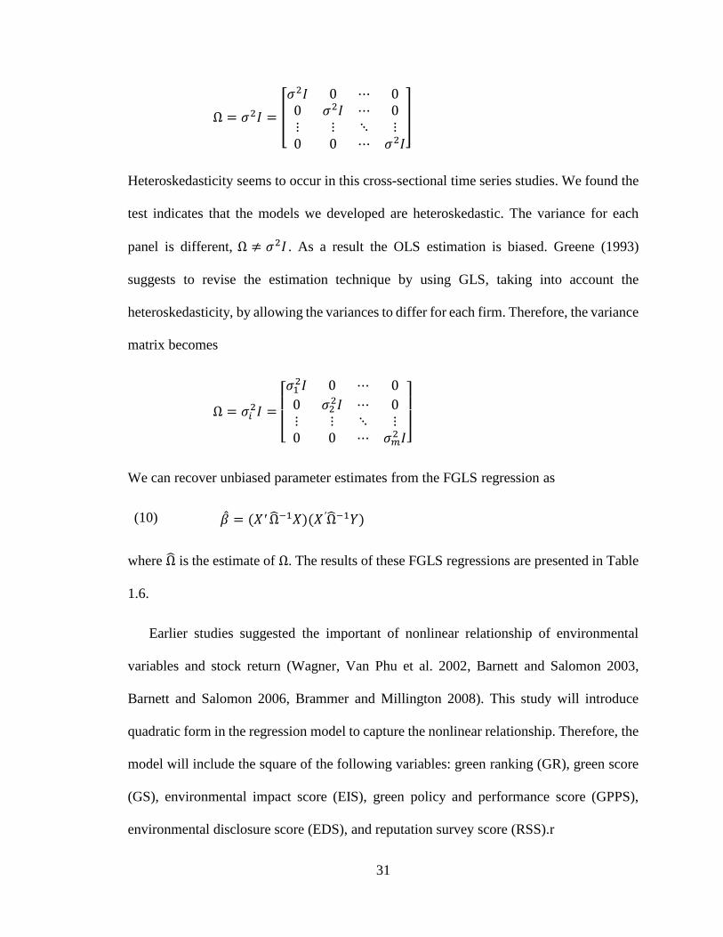
Heteroskedasticity seems to occur in this cross-sectional time series studies. We found the

test indicates that the models we developed are heteroskedastic. The variance for each

panel is different, Ω ≠ 𝜎2𝐼 . As a result the OLS estimation is biased. Greene (1993)

suggests to revise the estimation technique by using GLS, taking into account the

heteroskedasticity, by allowing the variances to differ for each firm. Therefore, the variance

matrix becomes

Ω = 𝜎𝑖2𝐼 =

[ 𝜎1

2𝐼 0 ⋯ 0

0 𝜎22𝐼 ⋯ 0

⋮ ⋮ ⋱ ⋮0 0 ⋯ 𝜎𝑚

2 𝐼]

We can recover unbiased parameter estimates from the FGLS regression as

(10) �̂� = (𝑋′ Ω̂−1𝑋)(𝑋′Ω̂−1𝑌)

where Ω̂ is the estimate of Ω. The results of these FGLS regressions are presented in Table

1.6.

Earlier studies suggested the important of nonlinear relationship of environmental

variables and stock return (Wagner, Van Phu et al. 2002, Barnett and Salomon 2003,

Barnett and Salomon 2006, Brammer and Millington 2008). This study will introduce

quadratic form in the regression model to capture the nonlinear relationship. Therefore, the

model will include the square of the following variables: green ranking (GR), green score

(GS), environmental impact score (EIS), green policy and performance score (GPPS),

environmental disclosure score (EDS), and reputation survey score (RSS).r

32

4. Results and Discussion

4.1. The general condition of the 500 largest public firms in the US in the sample

The sample for this study is the firms included in The Newsweek Green Ranking’s

sample from 2009 to 2012. The determination of the largest firms is based on revenue,

market capitalization and number of employees (Newsweek 2009). Because of this

screening some firms were purged in the proceeding samples. There are 56 firms in the

2009 sample that were replaced with new firms in 2010. Out of 500 firms in the 2010

sample, 36 firms were replaced with new firms in 2011. Out of 500 firms in the 2011

sample, 24 firms were replaced with new firms in 2012 sample. Overall, only 404 firms

are included in all four years. See Table 1.2.

Table 1.3 and 1.4 depict a general description of the firms’ characteristics and

performances of firms in the sample.

Stock Return (%) measures the three months cumulative raw return of firms’ stock

performances. Over the period of study, the stock returns experience ups and down. In the

first three years, the years soon following the great recession of 2008, the stock returns

improved dramatically from single digit, 7.93%, to double digit in two consecutive years

of 14.04% and 13.62% respectively in 2010 and 2011. However, the stock return then

dropped dramatically to only 4.73% in 2012, the period when stock market captured the

Dow Jones Industrial (DJI) stock price index to pre-recession level. The variability of

return among the 500 firms are huge with the range of about 250% for all first three years

and even wider in the year 2012, i.e. about 430%. The stock return is also slightly higher

as firms ranked higher in their green ranking over the period of study.

33

Market Risk (Beta Coefficient) measures the riskiness of a stock. The average level of

market risk is slightly lower from, 1.17 to 1.14, from 2009 to 2011. The market risk was

significantly lower as the stock market recaptured its DOW index to pre-recession level.

The risk level seems to be elevated slightly for firms with higher green ranking.

Market Capitalization ($ Billion) measures the size of firms. Over the period of the

study, the size of the firms increased significantly from the average level of $20 billion in

the beginning of the study in 2009 to $26 billion in 2012, over a four year period. The

largest firm in the sample doubled in size from $322 billion to $626 billion. Over the period

of 2009-2012 the market cap was also higher among firms with higher green ranking.

Annual Profit Growth (%) measures percentage change of earnings before tax and

interest (EBIT) over the previous year. In 2009, following 2008 recession, the profit of 288

firms out of the 500 largest firms in the US decreased on average of 16%, with the lowest

drop by 0.21% to the highest drop of 2,088%. The number of firms in the red reduced by

a half in the following year. That makes the average profit growth increased by 35%, 13%,

and 7% in 2010, 2011, and 2012 respectively.

4.2. Overall Hedonic Stock Price Model Estimates

Table 1.6 presents the complete results of the regression analysis. The model

estimations are separated into three parts, the periods of 2009-2010, 2011-2012, and 2009-

2012. The model estimation for the overall period of 2009-2012 only include the green

ranking (GR), the environmental impact score (EIS), and the green policy and performance

score (GPPS)9. The results show overall goodness of fit of the models. First, the accuracy

9 The estimation of the models is separated into three different time periods, i.e. 2009-2010, 2011-2012,

and 2009-2012. The main reason is Newsweek changed one of three specific measures of greenness in

34

of the model shown by the Wald-Chi-Square statistics indicates that the models are

efficient; all models are significant at 1% level of significance. Second, after transforming

some variables using centered value10, the tests of the models show that multicollinearity

is minimized in the models indicated by low Variance Inflation Factor (VIF) of the

variables in the right hand side of the equations to below 10. Third, as consequence of

transforming some variables to the deviation to their mean, the regression coefficients do

not represent the marginal effect of the variable. See Appendix 1.1 for a mathematical

explanation on how to recover the marginal effect. Forth, the violation of homoscedasticity

is present in all models. The modified Wald’s Test for group-wise heteroskedaticity in

panel data test reject the null hypothesis at levels of significance at 1% (See Table 1.5). In

estimating the models, therefore, we use a Feasible Generalized Least Square (FGLS) to

recover non-biased parameter estimates by assuming heteroskedatic matrix of variance.

See Table 1.6.

4.3. The Effect of Firm and Stock Characteristics to the Stock Return

See Table 1.6 for reference. The risk factor (market beta), market capitalization,

and profit growth, as expected, are significant factors that affect stock return. The risk

factor shows a strong significant non-linear affect in all eight models, column 1 to 8. Since

we use the original value we can use the parameter estimates as its marginal effect. Each

unit of risk gives a boost in stock return increasing in decreasing rate. On average the

marginal effect of market (beta) risk is 3.44% to 5.76%. Please note that the value of beta

2011, replacing RSS with EDS. Since the two measures are conceptually different therefore this study

separated the time periods before and after the event. 10 Centered value of variable 𝑥, i.e. 𝑐𝑡𝑟𝑥, is defined as the deviation of variable 𝑥 from its

means, 𝑐𝑡𝑟𝑥 = 𝑥 − �̅�

35

market risk in this study ranges from 0 to 5, with one extreme outlier of beta of 16. The

average value is average of 1.14. This result is consistent with Amihud anf Mendelson

(1989) at least in the direction of association. Both indicate significant (positive) effect.

The magnitude of the parameter estimate in our study shows stronger effect, 3.44% to

5.76%, compared to 0.7%. There are several possible explanations for the differences.

First, this study uses a short run accumulated return of three months while the prior study

uses an average monthly return for one year of return. This study uses raw return while the

previous study uses excess return. This study uses data only included in the 500 largest

public firms in the US as its sample.

Table 1.6 depicts the effect of market capitalization, measuring the size of the

companies, to the stock return. All parameter estimates are significant and show non-linear

relationships, increasing in decreasing rate. The results, at least the direction of the

relationship, are consistent with previous studies (Amihud and Mendelson 1989, Jaffe,

Keim et al. 1989). The parameter estimates from this study are stronger compare to the

prior studies. Evaluating at the mean value, for every billion dollar increase/decrease of the

value of market capitalization, it will increase/decrease the stock return about 0.03%.

Finally, the effects of profit growth to the stock return are all significant at alpha of

0.007% to 0.02%. The direction of the relationship is consistent with previous studies that

show that profitability affects stock return positively (Lee and Zumwalt 1981, Peavy and

Goodman 1985).

4.4. The effect of Firm’s Green Performances to its Stock Return

Compared to other green measures of a firm environmental performances that focus

more on a specific measure, the Newsweek’s green scores provides both broad or aggregate

36

measure: green ranking ((GR) and green score (GS)), and detail or disaggregate measure:

(impact (EIS), policy (GPPS), disclosure (EDS), and reputation (RSS)). That allows this

study not only to look at the effect of broad measures of firms’ environmental performance,

but also to find out specific aspects of firms’ environmental performance, i.e.

environmental impact of firm operation (EIS), management policy (GPPS), environmental

image (RSS), and disclosure (EDS).

Table 1.6 depicts the regression results estimations with eight different models that

include environmental variables in quadratic forms. The environmental variables include

the green ranking (GR), the green score (GS), the environmental impact score (EIS), the

green policy and performance score (GPPS), the reputation survey score (RSS), and the

environmental disclosure score (EDS). Most regression coefficients are significant at level

of significance at 1% and one occasion at 10%. Only three estimates failed to reject the

null hypothesis and all of them are the square of environmental variables.

Green ranking (GR) effect on stock return. The firms in the sample was ranked 1 to

500, from lowest to highest environmental scores. We found that green ranking has a

significant effect on stock return. Previous studies that use green ranking as a measure of

a firm’s environmental consciousness show conflicting results. Some studies found

positive effects between green ranking and stock (Derwall, Guenster et al. 2005,

Yamaguchi 2008) and some did not find a significant relationship (Yamashita, Sen et al.

1999, Takeda and Tomozawa 2006, Anderson-Weir 2010). We confirm previous studies

that there is a positive relationship between green ranking and stock performances.

Furthermore, the relationship follows diminishing marginal return, non-linear. See Table

1.6 column 1, 4, and 7.

37

Since the regression was calculated using centered value to mitigate muticollinearity,

the interpretation of the result needs further explanation. Figure 1.4 Panel A shows the

simulated effect of green ranking (GR) to stock return for three different models: 2009-

2010, 2011-2012, and 2009-2012 model. The curves show that the effect of green ranking

(GR) increases for the low green ranking firms and decreases for high green ranking firms.

The inflection points for the three models are at green ranking (GR) of 110 (Model 1: 2009-

2010), 118 (Model 4: 2011-2012), and 160 (Model 7: 2009-2012) respectively. The

investor’s willingness to pay (WTP) for green a firm to the left of the inflection point is

positive, while for a firm to the right of the inflection point is negative.

Green score (GS) effect on stock return. Green score is a linear combination value of

EIS, GPPS, EIS, and RSS or EDS. The value ranges from the lowest of 1 to the highest of

100. We found significant relationship between green score (GS) and stock performance,

contrary to Anderson-Weir (2010)’s finding. The earlier study uses cross-sectional data of

2009 Newsweek Green Ranking; he did not find evidence that the green score (GS) effects

stock return. Different from Andeson-Weir’s study, this study uses short panel data and

includes a non-linear relationship between the variables. Moreover, we provide treatment

for potential econometric issues including heteroskedasticiy and multicolliearity. See Table

1.6 column 2 and 5.

Again, since the regression is using centered value to avoid multicollinearity, to

interpret the regression results refer to Figure 1.4 panel b and c. Both panels show that the

relationship follows diminishing marginal return, the investor’s willingness to pay (WTP)

for a greener firm increases at the lower level of green score (GS) and decreases as pass

the inflection point. The inflection point of green score (GS) 28 (model 5: 2011-2012). We

38

found linear relationship between green score (GS) and stock return for the model 2: 2009-

2010.

The effect of disaggregate environmental score: impact (EIS), management and policy

(GPPS), reputation (RSS), and disclosure (EDS). We found that most of the disaggregate

scores are statistically significant, affecting stock return. See Table 1.6 column 3, 6, and 8.

The results confirm previous findings for environmental impact (Konar and Cohen 1997,

Bosch, Eckard et al. 1998, Gupta and Goldar 2005, Bird, Hall et al. 2007), environmental

management and policy (Feldman, Soyka et al. 1997, Thomas 2001), and reputation

(Karpoff, Lott Jr et al. 2005) and disclosure (Rao and Hamilton III 1996).

The investor’s willingness to pay (WTP) of the environmental impact score (EIS)

increases before the infection point of 35 (Model 3: 2009-2010). Model 6: 2011-2012 and

Model 8: 2009-2012, even though the squared EIS are significant, they have inflection

point close to. For the management and policy score (GPPS) the investor’s WTP increases

before inflection point of 39 and 199 (Model 8: 2009-2012), and WTP decreases afterward.

The investor’s WTP for reputation score (RSS) increases before the inflection point of 64

(2009-2010 model) and the WTP decreases afterward. Finally, the investor’s WTP for

environmental disclosure score (EDS) increases before the inflection point of 4 (Model 6:

2011-2012) and decreases afterward.

Table 1.7 provides examples of a special case of investor’s willingness to pay (WTP)

for green ranking (GR) based on Model 7: 2009-2012. On average investor’s WTP for

greener firms on the bottom 25 green ranking is about 0.0184% higher stock price than

39

otherwise, but for greener firms on the top 25 green ranking is about 0.0185% lower stock

price than otherwise.11

For firm in the bottom 25 out of 500 green ranking, the majority are firms in the utility,

energy and material sectors of business: FirstEnergy, Monsanto, Amaren, etc. For investors

in FirstEnergy’s stock, for example, their willingness to pay (WTP) for a better green

ranking is 0.0186% higher stock price. That means an investor is willing to pay a greener

stock at 0.0186% higher stock price. From the firm’s point of view, improving ranking by

one ranking will increase its return on investment by 0.0185%. Assuming the dividend and

number of stocks in circulation remain constant, the firm’s value increased as measured by

market capitalization by 0.0185%. If FirstEnergy, with market capitalization of

approximately $14 billion in 20012, improved its green ranking by one it will increase the

firm’s value approximately $2.6 million. The improvement in green ranking, therefore,

rewards firms too.

The top 25 of 500 green performers, on the other hand, are dominated by firms in

Information and Technology sectors like Google, IBM, Dell, Intel, Cysco, HP, Microsoft,

etc. For investors who purchase Google stock, as an example, the investor’s willingness to

pay (WTP) for higher green ranking stock is lowers return on investment by 0.0185%. If

we assume the dividend and number of stock remain constant, the improvement of ranking

will lower the firm’s value by 0.0185%. For Google with market value of $200 billion in

2012, the improvement of green ranking by one level will cost the firm’s value

approximately $37 million.

11 Stock return is loosely defined as percentage change of stock price, assuming dividend remains constant.

40

Curvature of relationship between environmental performance and stock return. One

interesting, unexplored study is an examination of non-linear relationship between these

two variables. This notion was first suggested more than a decade ago by economists

(Wagner, Schaltegger et al. 2001, Wagner, Van Phu et al. 2002, Barnett and Salomon

2003), but only one study has attempted to explore the relationship (Barnett and Salomon

2006). This study found the relationship between environmental variable and stock return

follows increasing in decreasing rate (concave). Investors willing to pay for eco-friendly

stock at higher stock price if they are in the group of dirty firms or low green ranking. This

contradicts the result of the study by Barnett and Salomon. They found that the relationship

is decreasing in increasing rate (convex or U-shape). Unlike this study, Barnett and

Salomon used mutual fund data. The measure of environmental performance is how the

environmental screen is use in choosing stock included in a fund. The environmental

screens pose due burden for fund managers by weeding out firms that do not meet the

screen criteria, at the price of lower return. This study uses hedonic price model that is

allowing investors to choose a stock based on a firm’s financial and environmental

attributes. Unlike in the case of a mutual fund, we do not screen out any firms. Investors

will see all choices of firms available, i.e. the largest 500 U.S. firms.

4.5. Robustness Check for the Models

This study uses two attempts of robustness check: (1) Dividing data into three

different time periods in estimating the models, and (2) Using different month to

calculate stock return as dependent variable in estimating the model. The first robustness

check based on Table 1.6. Model 1, 2, and 3 are for the period of 2009-2010, Model 4,5,

and 6 are for period of 2011-2012, and model 7 and 8 are for period of 2009-2012. The

41

results of estimating the models shows strong indication of robust results, at least in the

direction of relationships.

The second robustness check is based on the result depicted in Table 1.7. The table

depicts the estimation of the model using stock return as dependent variables calculated

based on 1, 2, 3, 4, 5, and 6 month cumulative return. The results show that the models

we estimate are consistent and robust at least in term of the direction of the relationship.

Most of the variables in the models are significant at least at p<10% and most of the

direction of the relationship on parameter estimates are consistent. Since the

environmental variables were transformed using centered value, the direction of the

results may not reflect the actual relationship. To further perform robustness check,

simulated graph of environmental variables and stock return are presented in Figure 1.4.

The results show most of curves are consistent.

5. Conclusion

5.1. Summary of Results

This study attempts to estimate Rosen’s (1976) hedonic model to find out if firms’

green characteristics affect investor preference in buying stocks. The estimation follows

the concept of the capital assets pricing mode (CAPM). The firm’s green attributes are

measured using the Newsweek Green Ranking 2009-2012 which include the green score

(GS), the environmental impact score (EIS), the green policy and performance score

(GPPS), and the reputation survey score (RSS). In addition to green variables, we also

include control variables that are commonly used in the CAPM studies, including the

firm’s/stock’s risk and non-risk characteristics. Based on the hedonic model we can

42

calculate (recover) the investor’s willingness to pay (WTP) for a certain environmental

characteristic of a stock.

This study found that all known financial variables affecting stock return are

significant; we found that environmental variables are also significant. These findings will

add a new addition to the array of studies in the Capital Assets Pricing Model (CAPM).

More importantly, this study sheds light on a new application of the Rosen hedonic pricing

model in the stock market.

Practically, this study provides one piece of information both for the investors and

firms to make cost and benefit analyses. As measured in its increase of market

capitalization, a firm can recover the expected return on an investment to improve its

environmental conduct and performance. Investor can benefit by finding out how much

additional return he or she can earn by purchasing stock of a firm with better environmental

conduct and performance.

5.2. Future research Agenda

This study has shown significant contemporaneous relationships between corporate’s

environmental performance and stock return. From the results the value of willingness to

pay (WTP) can be derived. The use of revealed preference such as the hedonic model in

deriving the value of WTP employed a strong assumption of homogeneity of investors.

Such assumption may not be supported empirically. That is the main limitation of the

revealed preference study. Such assumption can be relaxed by using stated preference like

the use of choice experiment using conjoint analysis. In choice experiment, investor’s

characteristic like demographic, socio-economic, and risk preference, can be explored and

use them as determinant of portfolio choice. From the analysis we can test the heterogeneity

43

of investors. Moreover, we can estimate more accurately the value of willingness to pay

(WTP) of environmentally friendly attributes in investment choices like in mutual fund.

Copyright © 2014 Muhammad S. Ahmadin

44

Table 1. 1: Type and Model of Previous Studies

Shape of Relationship between Environmental Variable and Stock Performance

Dichotomous (Linear)

Non-linear

Significant Positive

Significant

Negative Not Significant

Type S

tudies

Event Studies

Klassen & McLaughlin (1996)

Rao (1996)

Konar & Cohen (1997)

Bosch, Eckard, & Lee (1998)

Gupta & Goldar (2004)

Karpoff et.al. (2005)

Nagayama & Takeda (2006)

Yamaguchi (2008)

Yamashita, Sen,

and Roberts (1999)

Takeda

&Tomozawa

(2006)

Anderson-Weir

(2010)

Portfolio Studies

Diltz (1995)

Cohen, Fenn, et.al. (1997)

Blank & Daniel (2002)

Derwall, Guenster, et.al.

(2005)

Kempf & Osthoff (2007)

Fillbeck &

Gorman (2004)

Fillbeck &

Gorman (2004)

Regression Studies

Feldman, Soyka et.al. (1996)

Thomas (2001): Policy

Ziegler, Schroeder, et.al.

(2008)

Vasal (2009)

Brammer,

Brooks et.al.

(2006)

Bird, Hall, et.al.

(2007)

Thomas (2001):

Conduct

Manescu (2011)

Barnet & Salomon

(2006)

Conjoint Studies Bauer & Smeets (2010)

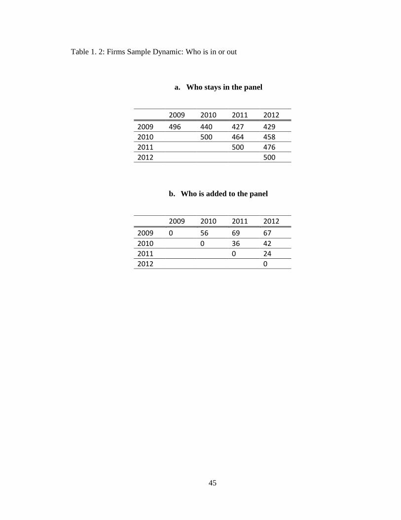
45

Table 1. 2: Firms Sample Dynamic: Who is in or out

a. Who stays in the panel

2009 2010 2011 2012

2009 496 440 427 429

2010 500 464 458

2011 500 476

2012 500

b. Who is added to the panel

2009 2010 2011 2012

2009 0 56 69 67

2010 0 36 42

2011 0 24

2012 0

46

Table 1. 3: Summary Statistic of Relevant Variables

*Green Ranking (GR) ranges from 1=the lowest rank, and 500=the highest rank

**Newsweek Green Ranking has been modified in 2011 and 2012 version, i.e. replacing

Reputation Survey Score (RSS) with Environmental Disclosure Score (EDS).

Variable Year Mean Std. Dev. Min Max Obs.2009 7.93 15.27 -50.52 200.85 492

2010 14.04 14.27 -42.04 189.02 494

2011 13.62 14.36 -88.18 61.36 496

2012 4.73 19.80 -47.14 380.86 498

2009 248.50 143.33 1 496 496

2010 250.50 144.48 1 500 500

2011 250.50 144.48 1 500 500

2012 250.50 144.48 1 500 500

2009 70.47 9.98 1 100 496

2010 70.54 11.11 1 100 500

2011 51.47 10.18 19.90 82.5 500

2012 53.24 10.40 21.40 82.90 500

2009 50.13 28.88 0.20 100 496

2010 50.45 28.65 1 100 500

2011 55.93 18.37 0.2 88.5 500

2012 56.39 18.38 0 89 500

2009 39.89 18.23 1 100 496

2010 42.22 19.32 1 100 500

2011 52.11 13.18 26.70 96.2 500

2012 53.64 13.89 21.30 91.9 500

2009 34.44 13.54 1 100 496

2010 47.46 14.02 1 100 500

2011 28.57 27.71 0 99.6 500

2012 37.31 30.95 0 100 500

2009 1.17 0.64 0.05 4.90 496

2010 1.12 0.40 0.31 2.68 500

2011 1.13 0.39 0.35 2.67 500

2012 1.14 0.83 0.01 16.52 500

2009 20.39 34.39 0.20 322.33 494

2010 23.15 38.23 0.31 364.06 496

2011 22.79 40.27 0.12 401.25 499

2012 25.83 48.83 0.26 626.55 492

2009 -16.32 128.06 -2081.19 669.23 478

2010 34.84 247.74 -2458.23 3125.30 481

2011 12.82 66.28 -471.46 947.17 487

2012 7.60 74.45 -384.26 928.81 493

Environmental Impact Score

(EIS)

Green Policy and Performance

Score (GPPS)

Stock Return (%)

Green Ranking (GR)*

Green Score (GS)**

Profit growth (%)

Market Risk (Beta)

Market Capitalization (Billion)

Reputation Survey Score (RSS)**

Environmental Disclosure Score

(EDS)**

47

Table 1. 4: The Firms’ Green Ranking Vs. Relevant Variables,

*Green Ranking (GR) ranges from 1 = the lowest rank, and 500 = the highest rank

**Newsweek Green Ranking has been modified in 2011 and 2012 version, i.e. replacing

Reputation Survey Score (RSS) with Environmental Disclosure Score (EDS)

Green Ranking* 2009 2010 2011 2012 Overall

401-500 7.74 11.81 10.16 4.67 4.67

301-400 10.29 15.66 13.53 6.36 6.36

201-300 6.94 15.61 15.48 5.42 5.42

101-200 6.59 12.66 12.13 3.06 3.06

001-100 8.09 14.55 16.92 4.19 4.19

Overall 7.93 14.04 13.62 4.73 4.73

401-500 1.28 1.03 1.03 1.34 1.19

301-400 1.21 1.18 1.18 1.01 1.15

201-300 1.24 1.20 1.20 1.05 1.15

101-200 1.21 1.10 1.10 1.18 1.13

001-100 0.94 1.09 1.09 1.13 1.08

Overall 1.17 1.12 1.12 1.14 1.14

401-500 39.93 48.00 43.01 14.24 36.48

301-400 22.69 26.30 22.40 19.95 22.84

201-300 12.06 15.27 17.29 17.30 15.53

101-200 15.01 13.52 18.96 29.23 19.08

001-100 12.72 12.12 12.14 48.03 21.27

Overall 20.39 23.15 22.79 25.83 23.04

401-500 -14.37 22.04 1.87 6.55 4.28

301-400 -21.01 -9.22 13.73 22.00 1.62

201-300 -24.03 72.06 8.29 1.40 14.40

101-200 -11.79 68.69 14.02 2.74 18.39

001-100 -10.53 19.63 26.07 5.25 10.03

Overall -16.32 34.84 12.82 7.60 9.77

Stock Return (%)

Market Capitalization(Billion $)

Market Beta Risk

Profit Growth (%)

Table 1. 5: Multicollinearity, Heteroskedasticity, and Autocorelation Test

Note: *Significant at P≤0.10; **significant at p P≤0.05; and *** significant at p P≤0.01

§The variable is modified to the difference from its mean value to mitigate collinearity

Before Before Before Before Before Before Before Before

Firm's Environmental Performances:Green ranking (GR) 52.42 1.15 § 38.01 1.09 § 39.01 1.10 §

Square of green ranking (GR2) 32.01 2.19 § 24.33 2.24 § 25.16 2.11 §

Green score (GS) 121.41 1.44 § 45.19 1.10 §

Square of green score (GS2) 82.97 1.46 § 24.95 1.52 §

Environmental Impact Score (EIS) 60.95 1.04 § 124.61 1.51 § 70.59 1.20 §

Square of Environmental Impact Score (EIS2) 34.91 2.11 § 61.64 1.73 § 39.51 1.94 §

Green Pol icy & Performance Score (GPPS) 67.15 1.35 § 79.53 1.85 § 48.79 1.18 §

Square of Green Pol icy & Performance Score (GPPS2) 30.40 1.75 § 31.19 1.99 § 23.31 1.69 §

Reputation Survey Score (RSS) 81.10 1.49 §

Square of Reputation Survey Score (RSS2) 30.77 1.73 §

Environmental Disclosure Score (EDS) 34.71 2.18 §

Square of Environmental Disclosure Score (EDS2) 22.63 2.72 §

Stock's Risk Characteristics:Beta Coeficient 21.97 10.07 46.49 8.26 48.39 10.94 6.99 3.19 11.33 2.49 12.83 4.20 6.66 2.82 9.61 3.25

Square of Beta Coeficient 9.33 7.04 15.40 6.51 16.34 7.07 2.48 1.72 3.14 1.63 3.32 1.91 2.05 1.58 2.31 1.64

Firm's Characteristics:Market Capita l i zation 1.01 1.01 8.32 1.01 8.85 8.15 4.85 4.56 5.16 4.49 5.50 4.70 4.79 4.59 4.98 4.37

Square of Market Capita l i zation (CAP2) 8.03 7.96 5.97 7.66 6.10 5.83 3.67 3.57 3.79 3.54 3.94 3.64 3.54 3.48 3.61 3.42

Profi t Growth (%) 5.86 5.84 1.01 5.72 1.01 1.01 1.03 1.03 1.03 1.03 1.04 1.04 1.01 1.01 1.01 1.01

AVERAGE 18.66 5.04 40.05 4.58 35.05 1.58 11.62 2.49 13.51 2.26 34.63 2.50 11.75 2.38 22.63 2.19

Wald's Chi -Square Test for Heterokedastici ty

- Ho: δ(i )2= δ

2 for a l l i

Wooldridge F-test for autocorrelation in panel data

- Ho: No AR(1)0.7238

1.40E+34

0.5310NA

*** 3.30E+33 *** 2.40E+35 ***2.60E+36

NA NA NA NA NA

1

***2.40E+36 *** 1.50E+35 *** 3.30E+35 ***3.10E+38 ***

After

2

After After

Variation Inflation Factor (VIF)After

5

AfterAfter

2011-20126

After After

74

2009-2010 2009-20123 8

48

Table 1. 6: The Estimation of Environmentally Friendly Hedonic Price Model

*Significant at P≤0.10; **significant at p P≤0.05; and *** significant at p P≤0.01. Due to multicolinearity, the following variables are

transformed to the deviation to their mean: all environmental variables. transformation, please be cautious in interpreting the regression

coefficients. See Figure 1.3 or Appendix 1.1 for the presentation of the simulation of the effect of each variable

Firm's Environmental Performances:

Green ranking (GR) -0.0030 *** -0.0089 *** -0.0051 ***

Square of green ranking (GR2) -1.12E-05 ** -3.36E-05 *** -2.82E-05 ***

Green score (GS) -0.0581 *** -0.1018 ***

Square of green score (GS2) -0.0001 -0.0021 ***

Environmental Impact Score (EIS) -0.0536 *** -0.0586 *** -0.0597 ***

Square of Environmental Impact Score (EIS2) -0.0003 *** -0.0005 ** -0.0005 ***

Green Pol icy & Performance Score (GPPS) -0.0020 -0.0996 *** -0.0633 ***

Square of Green Pol icy & Performance Score (GPPS2) -0.0006 * -7.74E-05 -0.0001

Reputation Survey Score (RSS) 0.0725 ***

Square of Reputation Survey Score (RSS2) -0.0016 ***

Environmental Disclosure Score (EDS) -0.0155 *

Square of Environmental Disclosure Score (EDS2) -0.0002

Stock's Risk Characteristics:

Beta Coeficient 16.0597 *** 16.7233 *** 16.2300 *** 6.0812 *** 6.1862 *** 5.5687 *** 3.9713 *** 4.9343 ***

Square of Beta Coeficient -4.7709 *** -4.9507 *** -4.5881 *** -0.3516 *** -0.3595 *** -0.3309 *** -0.2341 *** -0.2959 ***

Firm's Characteristics:

Market Capita l i zation 4.24E-05 *** 4.19E-05 *** 3.78E-05 *** 1.93E-05 *** 2.52E-05 *** 3.35E-05 *** 2.88E-05 *** 3.85E-05 ***

Square of Market Capita l i zation (CAP2) -1.18E-10 *** -1.18E-10 *** -1.18E-10 *** -9.45E-11 *** -1.03E-10 *** -1.16E-10 *** -1.13E-10 *** -1.27E-10 ***

Profi t Growth (%) 0.0077 *** 0.0076 *** 0.0058 *** 0.0202 *** 0.0179 *** 0.0175 *** 0.0080 *** 0.0076 ***

Constant -0.4768 -1.1436 ** -0.2780 3.1458 *** 2.5976 *** 2.9484 *** 5.8464 *** 4.5244 ***

Number of observations (N) 958 958 958 972 972 972 1930 1930

Time period (T) 2 2 2 2 2 2 4 4

Wald's Chi -Square 749 *** 875 *** 5629 *** 4941 *** 1538 *** 1447 *** 142 *** 405 ***

5 6 7 8Dependent Variable: Stock Return

2009-2010 2011-2012 2009-20121 2 3 4

49

Table 1. 7: The Willingness to Pay (WTP)* of Environmentally Friendliness

*was calculated using the following formula: 𝑊𝑇𝑃 = 𝐵 − 2𝐶�̅� + 2𝐶𝑥 where B and C are the parameter estimates for the variables and

their square respectively and x is the independent variables. See Figure 1 4.

Company Name SectorGreen

RankingWTP (%) Company Name Sector

Green

RankingWTP (%)

BlackRock Financials 1 0.0191 Allergan Healthcare 476 -0.0178

Alpha Natural Resources Energy 2 0.0191 American Express Financials 477 -0.0179

CF Industries Holdings Materials 3 0.0190 Best Buy Retailers 478 -0.0179

T. Rowe Price Group Financials 4 0.0189 Google Information Technology & Services 479 -0.0180

Monsanto Materials 5 0.0189 Autodesk Information Technology & Services 480 -0.0180

Invesco Financials 6 0.0188 Motorola Solutions Technology Equipment 481 -0.0181

CONSOL Energy Energy 7 0.0188 Cisco Systems Technology Equipment 482 -0.0182

Peabody Energy Energy 8 0.0187 Baxter Healthcare 483 -0.0182

Archer-Daniels-Midland Food, Beverage & Tobacco 9 0.0187 Citigroup Financials 484 -0.0183

FirstEnergy Utilities 10 0.0186 Manpower Professional Services 485 -0.0183

Tyson Foods Food, Beverage & Tobacco 11 0.0185 McGraw-Hill Media & Publishing 486 -0.0184

Ralcorp Holdings Food, Beverage & Tobacco 12 0.0185 Hartford Financial Services Grp. Financials 487 -0.0184

Ameriprise Financial Financials 13 0.0184 Cognizant Technology Information Technology & Services 488 -0.0185

Allegheny Technologies Materials 14 0.0184 Microsoft Information Technology & Services 489 -0.0185

AES Utilities 15 0.0183 EMC Technology Equipment 490 -0.0186

Ameren Utilities 16 0.0183 Staples Retailers 491 -0.0187

PPL Utilities 17 0.0182 Office Depot Retailers 492 -0.0187

Mead Johnson Nutrition Food, Beverage & Tobacco 18 0.0182 Accenture Information Technology & Services 493 -0.0188

Bunge Food, Beverage & Tobacco 19 0.0181 Intel Technology Equipment 494 -0.0188

Edison International Utilities 20 0.0180 Nvidia Technology Equipment 495 -0.0189

SCANA Utilities 21 0.0180 CA Technologies Information Technology & Services 496 -0.0189

Airgas Materials 22 0.0179 Dell Technology Equipment 497 -0.0190

Nucor Materials 23 0.0179 Sprint Nextel Telecommunications 498 -0.0191

Lorillard Food, Beverage & Tobacco 24 0.0178 Hewlett-Packard Technology Equipment 499 -0.0191

Precision Castparts Aerospace & Defense 25 0.0178 IBM Information Technology & Services 500 -0.0192

The Bottom 25 Firms in 2012 The Top 25 Firms in 2012

50

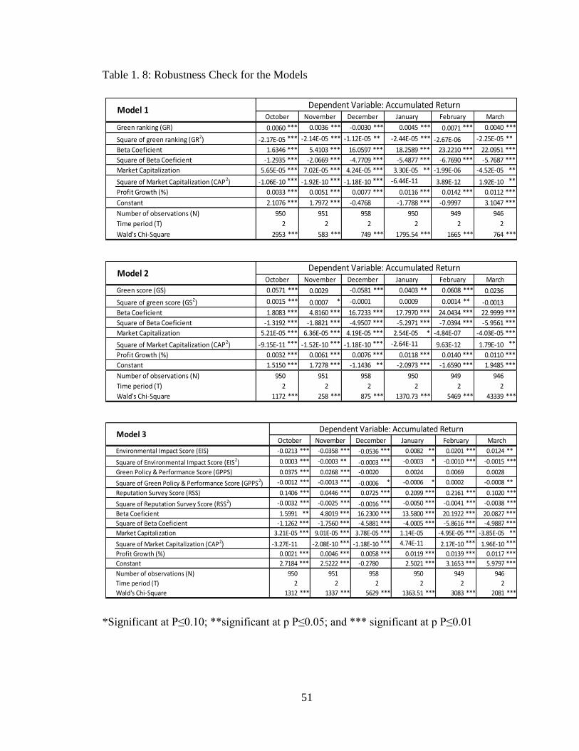
51

Table 1. 8: Robustness Check for the Models

*Significant at P≤0.10; **significant at p P≤0.05; and *** significant at p P≤0.01

Green ranking (GR) 0.0060 *** 0.0036 *** -0.0030 *** 0.0045 *** 0.0071 *** 0.0040 ***

Square of green ranking (GR2) -2.17E-05 *** -2.14E-05 *** -1.12E-05 ** -2.44E-05 *** -2.67E-06 -2.25E-05 **

Beta Coeficient 1.6346 *** 5.4103 *** 16.0597 *** 18.2589 *** 23.2210 *** 22.0951 ***

Square of Beta Coeficient -1.2935 *** -2.0669 *** -4.7709 *** -5.4877 *** -6.7690 *** -5.7687 ***

Market Capitalization 5.65E-05 *** 7.02E-05 *** 4.24E-05 *** 3.30E-05 ** -1.99E-06 -4.52E-05 **

Square of Market Capitalization (CAP2) -1.06E-10 *** -1.92E-10 *** -1.18E-10 *** -6.44E-11 3.89E-12 1.92E-10 **

Profit Growth (%) 0.0033 *** 0.0051 *** 0.0077 *** 0.0116 *** 0.0142 *** 0.0112 ***

Constant 2.1076 *** 1.7972 *** -0.4768 -1.7788 *** -0.9997 3.1047 ***

Number of observations (N) 950 951 958 950 949 946

Time period (T) 2 2 2 2 2 2

Wald's Chi-Square 2953 *** 583 *** 749 *** 1795.54 *** 1665 *** 764 ***

January

Dependent Variable: Accumulated Return Model 1

October November December February March

Green score (GS) 0.0571 *** 0.0029 -0.0581 *** 0.0403 ** 0.0608 *** 0.0236

Square of green score (GS2) 0.0015 *** 0.0007 * -0.0001 0.0009 0.0014 ** -0.0013

Beta Coeficient 1.8083 *** 4.8160 *** 16.7233 *** 17.7970 *** 24.0434 *** 22.9999 ***

Square of Beta Coeficient -1.3192 *** -1.8821 *** -4.9507 *** -5.2971 *** -7.0394 *** -5.9561 ***

Market Capitalization 5.21E-05 *** 6.36E-05 *** 4.19E-05 *** 2.54E-05 * -4.84E-07 -4.03E-05 ***

Square of Market Capitalization (CAP2) -9.15E-11 *** -1.52E-10 *** -1.18E-10 *** -2.64E-11 9.63E-12 1.79E-10 **

Profit Growth (%) 0.0032 *** 0.0061 *** 0.0076 *** 0.0118 *** 0.0140 *** 0.0110 ***

Constant 1.5150 *** 1.7278 *** -1.1436 ** -2.0973 *** -1.6590 *** 1.9485 ***

Number of observations (N) 950 951 958 950 949 946

Time period (T) 2 2 2 2 2 2

Wald's Chi-Square 1172 *** 258 *** 875 *** 1370.73 *** 5469 *** 43339 ***

February MarchModel 2

Dependent Variable: Accumulated Return October November December January

Environmental Impact Score (EIS) -0.0213 *** -0.0358 *** -0.0536 *** 0.0082 ** 0.0201 *** 0.0124 **

Square of Environmental Impact Score (EIS2) 0.0003 *** -0.0003 ** -0.0003 *** -0.0003 * -0.0010 *** -0.0015 ***

Green Policy & Performance Score (GPPS) 0.0375 *** 0.0268 *** -0.0020 0.0024 0.0069 0.0028

Square of Green Policy & Performance Score (GPPS2) -0.0012 *** -0.0013 *** -0.0006 * -0.0006 * 0.0002 -0.0008 **

Reputation Survey Score (RSS) 0.1406 *** 0.0446 *** 0.0725 *** 0.2099 *** 0.2161 *** 0.1020 ***

Square of Reputation Survey Score (RSS2) -0.0032 *** -0.0025 *** -0.0016 *** -0.0050 *** -0.0041 *** -0.0038 ***

Beta Coeficient 1.5991 ** 4.8019 *** 16.2300 *** 13.5800 *** 20.1922 *** 20.0827 ***

Square of Beta Coeficient -1.1262 *** -1.7560 *** -4.5881 *** -4.0005 *** -5.8616 *** -4.9887 ***

Market Capitalization 3.21E-05 *** 9.01E-05 *** 3.78E-05 *** 1.14E-05 -4.95E-05 *** -3.85E-05 **

Square of Market Capitalization (CAP2) -3.27E-11 -2.08E-10 *** -1.18E-10 *** 4.74E-11 2.17E-10 *** 1.96E-10 ***

Profit Growth (%) 0.0021 *** 0.0046 *** 0.0058 *** 0.0119 *** 0.0139 *** 0.0117 ***

Constant 2.7184 *** 2.5222 *** -0.2780 2.5021 *** 3.1653 *** 5.9797 ***

Number of observations (N) 950 951 958 950 949 946

Time period (T) 2 2 2 2 2 2

Wald's Chi-Square 1312 *** 1337 *** 5629 *** 1363.51 *** 3083 *** 2081 ***

Model 3Dependent Variable: Accumulated Return

October November December January February March

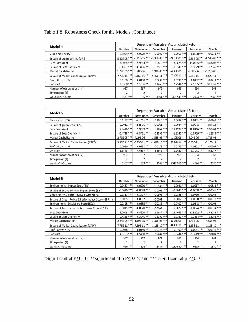
52

Table 1.8: Robustness Check for the Models (Continued)

*Significant at P≤0.10; **significant at p P≤0.05; and *** significant at p P≤0.01

Green ranking (GR) -0.0099 *** -0.0099 *** -0.0089 *** -0.0065 *** -0.0050 *** 0.0031 **

Square of green ranking (GR2) -5.47E-05 *** -6.81E-05 *** -3.36E-05 *** -9.10E-05 *** -9.53E-05 *** -8.54E-05 ***

Beta Coeficient 7.3024 *** 5.9553 *** 6.0812 *** 18.0878 *** 19.0565 *** 16.8207 ***

Square of Beta Coeficient -0.4357 *** -0.3406 *** -0.3516 *** -1.3141 *** -1.3829 *** -1.2549 ***

Market Capitalization 1.79E-05 *** 6.48E-06 1.93E-05 *** -4.38E-06 -5.38E-06 -1.71E-05

Square of Market Capitalization (CAP2) -7.72E-11 *** -6.66E-11 *** -9.45E-11 *** -7.20E-11 * -5.61E-11 -5.52E-11

Profit Growth (%) 0.0108 ** 0.0198 *** 0.0202 *** 0.0190 *** 0.0132 *** 0.0211 ***

Constant 3.5380 *** 5.1096 *** 3.1458 *** 2.2144 *** 4.1365 *** 10.1037 ***

Number of observations (N) 967 967 972 965 964 963

Time period (T) 2 2 2 2 2 2

Wald's Chi-Square 531 *** 335 *** 4941 *** 4652.45 *** 2424 *** 2186 ***

Model 4Dependent Variable: Accumulated Return

October November December January February March

Green score (GS) -0.1197 *** -0.1001 *** -0.1018 *** -0.0692 *** -0.0491 *** 0.0242 **

Square of green score (GS2) -0.0031 *** -0.0025 *** -0.0021 *** -0.0044 *** -0.0048 *** -0.0041 ***

Beta Coeficient 7.8616 *** 5.9589 *** 6.1862 *** 18.1994 *** 18.8146 *** 17.0204 ***

Square of Beta Coeficient -0.4738 *** -0.3461 *** -0.3595 *** -1.3242 *** -1.3709 *** -1.2685 ***

Market Capitalization 2.71E-05 *** 4.19E-06 2.52E-05 *** 1.10E-06 -4.74E-06 -1.73E-05

Square of Market Capitalization (CAP2) -9.55E-11 *** -6.29E-11 *** -1.03E-10 *** -9.02E-11 ** -5.13E-11 -5.17E-11

Profit Growth (%) 0.0086 *** 0.0181 *** 0.0179 *** 0.0193 *** 0.0152 *** 0.0207 ***

Constant 2.9445 *** 4.4897 *** 2.5976 *** 1.2421 *** 3.7071 *** 9.2077 ***

Number of observations (N) 967 967 972 965 964 963

Time period (T) 2 2 2 2 2 2

Wald's Chi-Square 5567 *** 359 *** 1538 *** 25427.66 *** 4594 *** 2070 ***

Model 5Dependent Variable: Accumulated Return

October November December January February March

Environmental Impact Score (EIS) -0.0687 *** -0.0990 *** -0.0586 *** -0.0961 *** -0.0917 *** -0.0531 ***

Square of Environmental Impact Score (EIS2) -0.0016 *** -0.0028 *** -0.0005 ** -0.0045 *** -0.0058 *** -0.0045 ***

Green Policy & Performance Score (GPPS) -0.1537 *** -0.1707 *** -0.0996 *** -0.0828 *** -0.0790 *** -0.0062

Square of Green Policy & Performance Score (GPPS2) -0.0005 -0.0002 -0.0001 -0.0007 * -0.0030 *** -0.0022 ***

Environmental Disclosure Score (EDS) 0.0395 *** 0.0385 *** -0.0155 * 0.0402 *** 0.0348 *** 0.0106

Square of Environmental Disclosure Score (EDS2) -0.0015 *** -0.0020 *** -0.0002 -0.0027 *** -0.0024 *** -0.0024 ***

Beta Coeficient 6.9095 *** 6.4309 *** 5.5687 *** 16.4063 *** 17.5592 *** 17.2753 ***

Square of Beta Coeficient -0.4215 *** -0.3846 *** -0.3309 *** -1.2286 *** -1.3114 *** -1.2981 ***

Market Capitalization 2.24E-05 *** 1.69E-05 *** 3.35E-05 *** -8.68E-06 -1.43E-05 -4.55E-06

Square of Market Capitalization (CAP2) -7.76E-11 *** -7.89E-11 *** -1.16E-10 *** -8.03E-11 ** -1.63E-11 -1.10E-10 *

Profit Growth (%) 0.0038 0.0140 *** 0.0175 *** 0.0190 *** 0.0081 ** 0.0175 ***

Constant 4.6703 *** 6.5490 *** 2.9484 *** 6.0444 *** 9.3919 *** 12.8404 ***

Number of observations (N) 967 967 972 965 964 963

Time period (T) 2 2 2 2 2 2

Wald's Chi-Square 656 *** 924 *** 1447 *** 2508.30 *** 6865 *** 1930 ***

Model 6Dependent Variable: Accumulated Return

October November December January February March

53

Table 1.8: Robustness Check for the Models (Continued)

*Significant at P≤0.10; **significant at p P≤0.05; and *** significant at p P≤0.01

Green ranking (GR) -0.0045 *** -0.0045 *** -0.0051 *** -0.0008 -0.0014 0.0045 ***

Square of green ranking (GR2) -3.13E-05 *** -4.20E-05 *** -2.82E-05 *** -5.72E-05 *** -5.16E-05 *** -4.81E-05 ***

Beta Coeficient 1.8617 *** 2.6018 *** 3.9713 *** 10.7362 *** 11.4900 *** 11.6640 ***

Square of Beta Coeficient -0.1161 *** -0.1419 *** -0.2341 *** -0.8922 *** -0.9561 *** -0.9584 ***

Market Capita l i zation 2.10E-05 *** 2.00E-05 *** 2.88E-05 *** 2.51E-05 *** 1.02E-05 -1.98E-05

Square of Market Capita l i zation (CAP2) -6.30E-11 *** -7.86E-11 *** -1.13E-10 *** -1.43E-10 *** -9.65E-11 * -3.51E-11

Profi t Growth (%) 0.0041 *** 0.0083 *** 0.0080 *** 0.0116 *** 0.0145 *** 0.0142 ***

Constant 4.6935 *** 5.4978 *** 5.8464 *** 4.5849 *** 7.5152 *** 10.9790 ***

Number of observations (N) 1917 1918 1930 1915 1913 1909

Time period (T) 4 4 4 4 4 4

Wald's Chi -Square 102 *** 220 *** 142 *** 814.76 *** 6355 *** 660 ***

October November December January February MarchModel 7

Dependent Variable: Accumulated Return

Environmental Impact Score (EIS) -0.0128 *** -0.0336 *** -0.0597 *** 0.0048 -0.0024 0.0177 *

Square of Environmental Impact Score (EIS2) -0.0018 *** -0.0018 *** -0.0005 *** -0.0022 *** -0.0033 *** -0.0033 ***

Green Pol icy & Performance Score (GPPS) -0.0330 *** -0.0372 *** -0.0633 *** -0.0121 -0.0022 0.0130

Square of Green Pol icy & Performance Score (GPPS 2) -0.0013 *** -0.0008 *** -0.0001 -0.0001 -0.0009 ** -0.0003

Beta Coeficient 1.9654 *** 2.5631 *** 4.9343 *** 9.5868 *** 11.1867 *** 11.1114 ***

Square of Beta Coeficient -0.1270 *** -0.1484 *** -0.2959 *** -0.8322 *** -0.9447 *** -0.9412 ***

Market Capita l i zation 2.51E-05 *** 2.22E-05 *** 3.85E-05 *** 1.35E-05 -1.45E-05 -3.11E-05 **

Square of Market Capita l i zation (CAP2) -7.57E-11 *** -8.07E-11 *** -1.27E-10 *** -1.27E-10 *** -3.11E-11 -1.55E-11

Profi t Growth (%) 0.0063 *** 0.0086 *** 0.0076 *** 0.0134 *** 0.0154 *** 0.0120 ***

Constant 5.6957 *** 6.1318 *** 4.5244 *** 5.7787 *** 9.2631 *** 12.9878 ***

Number of observations (N) 1917 1918 1930 1915 1913 1909

Time period (T) 4 4 4 4 4 4

Wald's Chi -Square 64909 *** 484 *** 405 *** 790.24 *** 1073 *** 1231 ***

Model 8Dependent Variable: Accumulated Return

October November December January February March

54

Figure 1. 1: A Market for a Typical Stock with Elastic Demand Curve

Source: Modified from Johnson and Lambert (1965), Levin and Wright (2002), and Hall and Lieberman (2010)

55

Figure 1. 2: A Market for a Typical Stock with Perfectly Elastic Demand Curve

Source: Modified from Johnson and Lambert (1965), Levin and Wright (2002), and Hall and Lieberman (2010)

56

Figure 1. 3: The Simulated effect of The Firms’ Environmental Attributes to Stock Return

a. Green Ranking (GR)

b. Environmental Scores 2009-2010

c. Environmental Scores 2011-2012

d. Environmental Scores 2009-2012

Note: Based on FGLS Estimation, given all other variables constant at mean values.

Environmental Attributes include: Green Ranking (GR), Green Score (GS), Environmental

Impact Score (EIS), Reputation Survey Score (RSS), and Environmental Disclosure Score

(EDS)

67

89

10

11

Sto

ck R

etu

rn (

%)

0 100 200 300 400 500The Firm Evironmental Ranking, 500=The Greenest

2009-2010 2011-2012

2009-2012

68

10

12

14

Sto

ck R

etu

rn (

%)

0 20 40 60 80 100The Firm Evironmental Score, 100=The Greenest

GS EIS

GPPS RSS

05

10

15

Sto

ck R

etu

rn (

%)

0 20 40 60 80 100The Firm Evironmental Score, 100=The Greenest

GS EIS

GPPS EDS

68

10

12

Sto

ck R

etu

rn (

%)

0 20 40 60 80 100The Firm Evironmental Score, 100=The Greenest

EIS GPPS

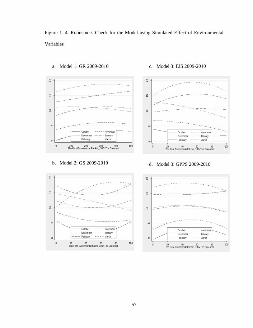
57

Figure 1. 4: Robustness Check for the Model using Simulated Effect of Environmental

Variables

a. Model 1: GR 2009-2010

b. Model 2: GS 2009-2010

c. Model 3: EIS 2009-2010

d. Model 3: GPPS 2009-2010

05

10

15

20

Sto

ck R

etu

rn (

%)

0 100 200 300 400 500The Firm Evironmental Ranking, 500=The Greenest

October November

December January

February March

05

10

15

20

Sto

ck R

etu

rn (

%)

0 20 40 60 80 100The Firm Evironmental Score, 100=The Greenest

October November

December January

February March

05

10

15

20

Sto

ck R

etu

rn (

%)

0 20 40 60 80 100The Firm Evironmental Score, 100=The Greenest

October November

December January

February March

05

10

15

20

Sto

ck R

etu

rn (

%)

0 20 40 60 80 100The Firm Evironmental Score, 100=The Greenest

October November

December January

February March

58

Figure 1. 4: Robustness Check of the Model using Simulated Effect of Environmental

Variables (Continued)

e. Model 3: RSS 2009-2010

f. Model 4: GR 2011-2012

g. Model 5: GS 2011-2012

h. Model 6: EIS 2011-2012

-10

010

20

Sto

ck R

etu

rn (

%)

0 20 40 60 80 100The Firm Evironmental Score, 100=The Greenest

October November

December January

February March

510

15

20

25

Sto

ck R

etu

rn (

%)

0 100 200 300 400 500The Firm Evironmental Ranking, 500=The Greenest

October November

December January

February March

05

10

15

20

25

Sto

ck R

etu

rn (

%)

0 20 40 60 80 100The Firm Evironmental Score, 100=The Greenest

October November

December January

February March

510

15

20

25

30

Sto

ck R

etu

rn (

%)

0 20 40 60 80 100The Firm Evironmental Score, 100=The Greenest

October November

December January

February March

59

Figure 1. 4: Robustness Check of the Model using Simulated Effect of Environmental

Variables (Continued)

j. Model 6: GPPS 2011-2012

k. Model 6: EDS 2011-2012

l. Model 7: GR 2009-2012

m. Model 8: EIS 2009-2012

05

10

15

20

25

Sto

ck R

etu

rn (

%)

0 20 40 60 80 100The Firm Evironmental Score, 100=The Greenest

October November

December January

February March

510

15

20

25

30

Sto

ck R

etu

rn (

%)

0 20 40 60 80 100The Firm Evironmental Score, 100=The Greenest

October November

December January

February March

510

15

20

25

Sto

ck R

etu

rn (

%)

0 100 200 300 400 500The Firm Evironmental Ranking, 500=The Greenest

October November

December January

February March

510

15

20

25

Sto

ck R

etu

rn (

%)

0 20 40 60 80 100The Firm Evironmental Score, 100=The Greenest

October November

December January

February March

60

Figure 1. 4: Robustness Check of the Model using Simulated Effect of Environmental

Variables (Continued)

n. Model 8: GPPS: 2009-2012

05

10

15

20

Sto

ck R

etu

rn (

%)

0 20 40 60 80 100The Firm Evironmental Score, 100=The Greenest

October November

December January

February March

61

Appendix 1. 1: Deriving Marginal effect based on centered value regression

Suppose we have regression of

(11) 𝑦 = 𝑎 + 𝑏𝑥 + 𝑐𝑥2 + 𝑒

Because of multicolinearity among the variables on the right hand side therefore we

estimate the regression by using centered-value of the independent variables.

(12) 𝑦 = 𝐴 + 𝐵(𝑥 − �̅�) + 𝐶(𝑥 − �̅�)2 + 𝐸

From the regression estimate we have the estimate of parameter A, B, and C from

equation (12). To recover the value of a, b, and c from equation (11) therefore we need to

rearrange deterministic part of the parameter estimates from the right hand side of

equation (12).

(13) 𝑦 = 𝐴 + 𝐵𝑥 − 𝐵�̅� + 𝐶(𝑥2 − 2𝑥�̅� + �̅�2) = 𝐴 + 𝐵𝑥 − 𝐵�̅� + 𝐶𝑥2 − 2𝐶𝑥�̅� + 𝐶�̅�2 = 𝐵𝑥 + 𝐶𝑥2 − 2𝐶𝑥�̅� + (𝐴 + 𝐶�̅�2 − 𝐵�̅�) = (𝐴 + 𝐶�̅�2 − 𝐵�̅�) + (𝐵 − 2𝐶�̅�)𝑥 + 𝐶𝑥2

Therefore,

a=(𝐴 + 𝐶�̅�2 − 𝐵�̅�)

b=(𝐵 − 2𝐶�̅�)

c=C

The value of marginal effect or willingness to pay (WTP) is given by the following.

(14) 𝑀𝑎𝑟𝑔𝑖𝑛𝑎𝑙 𝐸𝑓𝑓𝑒𝑐𝑡 = 𝑊𝑇𝑃 =

𝑑𝑦

𝑑𝑥= (𝐵 − 2𝐶�̅�) + 2𝐶𝑥

(15) 𝐼𝑛𝑓𝑙𝑒𝑐𝑡𝑖𝑜𝑛 𝑝𝑜𝑖𝑛𝑡 = (𝐵 − 2𝐶�̅�)/−2𝐶

Copyright © 2014 Muhammad S. Ahmadin

62

Chapter 3: The Effect of Firm’s Environmental Performances on Its Market Risk

1. Introduction

A firm’s environmental conduct can have an obvious effect on the firm’s stock

systematic risk level; which is the co-movement of a stock return and the stock market

return which measures an undiversified riskiness of a stock. For example, the British

Petroleum (BP) gulf oil spill in early 2010 increased BP’s stock volatility between two to

four times higher than pre-disaster (Fodor and Stowe 2010). However, such an extreme

type of event seldom occurs; typical events are more subtle and seamless. There are

numerous measures which provide information on the level of firms’ environmentally risky

behaviors, like information about the environmental impact of a firm’s operation, the

sophistication, or lack thereof, of a firm policy dealing with environmental issues, or in the

form of a report on people’s perception, including expert evaluation, of a firm

environmental conduct. Studies show that given such information, investors respond

immediately to such information as they are published (Klassen and McLaughlin 1996,

Konar and Cohen 1997).

The intriguing question is whether such information about a firms’ environmental

performance can affect their future stock systematic risk. Knowing this relationship will be

useful for investors in predicting the riskiness of an investment to maximize utility. There

are numerous studies attempting to investigate the effect of a firm’s environmental conduct

to a firm’s stock systematic risk. Some studies argue that economic factors play an

important role in shaping the financial risk (Rosenberg and Guy 1976); some show that a

firm’s environmental policy and conducts can mitigate the riskiness of a firm’s stock, while

63

the others argue that this measure will add cost to the firm (Spicer 1978, Feldman, Soyka

et al. 1996).

The purpose of this study is to determine whether a firm’s environmental

performance affects its future systematic risk. We attempt to investigate the causal

relationship between environmental and systematic risk performances. Importantly, this

study addresses the issue of non-linearity relationship between environmental and risk

performance as suggested by several studies (Wagner, Schaltegger et al. 2001, Wagner,

Van Phu et al. 2002, Barnett and Salomon 2003). This study uses data from the Newsweek

Green Ranking of the 500 largest US firms and follow them from 2009 to 2012, which

provide information reports on a firms’ environmental conduct and performances. In brief,

the results show a significant non-linear relationship (U-shape) between environmental

conduct and systematic risk. For the 25 firms in the worst environmental ranking, every

improvement of green ranking by a point in rank reduces systematic risk around 0.2%.

The remainder of this report will proceed as the following: (1) A review of previous

studies that will provide a framework for empirical tests including the use of control

variables; (2) Presentation of a methodological approach that will outline the organization

of the hypothesis testing; (3) Results and discussion are presented and a conclusion will be

drawn.

2. Literature Review

2.1. Firm’s Market (Beta) Risk

In any portfolio choice, investors are exposed to systematic and unsystematic risks.

The un-systematic or idiosyncratic risk associated with the variability of a firm’s stock

itself is independent of the market in general. This risk measures the volatility of stock

64

price due to how a firm conducts itself, i.e. management culture and values, marketing

strategies: pricing, development, placement, etc. This type of risk can be minimized by

diversifying a portfolio.

The systematic risk, on the other hand, is a risk that cannot be avoided by

diversifying a portfolio. To avoid risk investors must give up return. The measure of the

systematic risk is market beta or market risk; the beta value shows the co-movement of a

stock’s price with the kernel of index of assets prices, the sensitivity of a stock price to the

market price.

Both risk measures, systematic and unsystematic risk, are derived from

equation (16) below, following Sharp (1964). One common measures of stock market price

is the stock index like the Standard and Poor’s 500.

(16) 𝑅𝑖𝑡 = 𝑎𝑖 + 𝐵𝑖𝑅𝑚𝑡 + 𝑒𝑖𝑡

where 𝑅𝑖𝑡 is a return of stock 𝑖 at time 𝑡 ; 𝑎𝑖 is the value of stock 𝑖 ’s return which

independent from market return; 𝐵𝑖 is the measure of systematic risk, the value of stock 𝑖’s

return which dependent on the market return; 𝑅𝑚𝑡 is the market return at time

𝑡 𝑜𝑓 𝑓𝑖𝑟𝑚 𝑚, and 𝑒𝑖𝑡 is the error term of stock 𝑖 at time 𝑡. Based on this regression we can

recover the standard deviation of error term for a stock and that is the measure of firm’s

idiosyncratic risk. Systematic risk accounts for about 20% of total risk, while idiosyncratic

risk accounts for about 80% of total risk (Goyal and Santa-Clara 2003, José‐Miguel Gaspar

and Massimo Massa 2006).

65

The value of stock systematic risk can be affected by several variables. To

investigate the effect of environmental factors on a firms’ stock this study will start from

the earlier models that explain the determinant of risk. Many studies show that the

systematic risks can be affected by firms’ financial condition like operating leverage, and

environmental factors.

2.2. Firms’ Financial Factors and risks profiles: the control variables

By definition market (beta) risk is affected by market wide events; events that

influence all stocks in the market, e.g. interest rate change, unemployment, etc. Firm

specific events like corporate financial condition, environmental conducts, etc., affects

idiosyncratic risk. Grouping the events into the two categories, however, is “highly

abstractive” (Beaver, Kettler et al. 1970). Empirically, the firm specific events also have

influence on shaping the market risk. It was Beaver, Kettler et al. (1970) who pioneered

linking the effect of corporate financial performances, i.e. accounting risk and market risk.

Based on Beaver et al.’s notions, Hamada (1972) further show theoretically that such a

firm specific events affect market risk.

The effect of a firm’s financial factors on its stock systematic risk has been well

documented in numerous studies. Hamada (1972) synthesized the capital asset pricing

model (CAPM)12 and the Modigliani and Miller (MM)13 theory; and showed and found

empirically that the value of the systematic risk should be greater for a stock of a firm

12 The efficient set of portfolios to any individual investor will always be some combination of lending at

risk-free rate and “market portfolio” Hamada, R. S. (1972). "The Effect of the Firm's Capital Structure on

the Systematic Risk of Common Stocks." The Journal of Finance 27(2): 435-452. 13 The value of a firm is unaffected by the way how the firm is financed, via personal or corporate

borrowing. .Modigliani, F. and H. M. Merton (1965). "The Cost of Capital, Corporation Finance, and the Theory of

Investment: Reply." The American Economic Review 55(3): 524-527.

66

which has high value of debt-equity ratio than that of a firm with low debt-equity ratio. His

study also found that firm’s leverage does significantly affect the firm’s stock systematic

risk.

To mitigate the heterogeneity issue across industry, Melicher (1974) conducted a

study in a homogenous industry sample and employed various measures of corporate

financial condition as determinants of systematic risk. The study confirmed Hamada’s

findings that there is a significant positive relationship between a firm’s financial leverage

and a firm’s stock systematic risk. The effects of the other variables on its stock beta are

also significant, including the lag of financial factors, the equity return, the firm size, and

dividend payout policy.

Beside finding the effect of financial leverage, like earlier studies, more recent

studies investigated the effect of operating leverage of a firm to its stock’s systematic risk

(Hill and Stone 1980, Mandelker and Rhee 1984, Huffman 1989). The studies used

different measures of operating risk. The results showed that both operating leverage and

financial leverage have a significant effect on the firm’s stock’s systematic risk. Moreover,

Hill and Stone (1980) found a nonlinear relationship between the firm’s financial leverage

and systematic risk. Mandelker and Rhee (1984) found that the firms engaged in a trade-

off between the degree of operating leverage14 and the degree of financial leverage15. In

more comprehensive measures, Iqbal and Shah (2012) showed that liquidity, assets

turnover, profitability, size, dividend payout, and equity value significantly affect

systematic risk.

14 𝑂𝐿 = (𝑆𝑎𝑙𝑒𝑠 − 𝑉𝑎𝑟𝑖𝑎𝑏𝑙𝑒 𝐶𝑜𝑠𝑡)/(𝑅𝑒𝑣𝑒𝑛𝑢𝑒 − 𝑉𝑎𝑟𝑖𝑎𝑏𝑙𝑒 𝐶𝑜𝑠𝑡 − 𝐹𝑖𝑥 𝐶𝑜𝑠𝑡) 15 𝐹𝐿 = 𝑇𝑜𝑡𝑎𝑙 𝐴𝑠𝑠𝑒𝑡𝑠/𝑆ℎ𝑎𝑟𝑒ℎ𝑜𝑙𝑑𝑒𝑟𝑠′𝐸𝑞𝑢𝑖𝑡𝑦

67

2.3. Firm’s Environmental and Systematic Risk Performances

2.3.1. Theoretical Argument

There has been growing interest in linking the effect of a firm’s environmental

conducts and the market risk. There are several theoretical arguments used in justifying the

effect of environmental factors to the systematic risk: the information disclosure theory

(Spicer 1978, Trotman and Bradley 1981, García-Ayuso and Larrinaga 2003), the financial

and profitability theory (Feldman, Soyka et al. 1996, Klassen and McLaughlin 1996), and

the stakeholder theory (Salama, Anderson et al. 2011). The accounting information

disclosure theory argues that disclosing a firm’s information reduces information

asymmetry which reduces systematic risk in investing. If investors are blindsided about a

firm’s condition they will put a premium to offset a potential cost that may occur in the

future in case a bad portfolio selection is made. Similarly, the environmental information

disclosure also reduces information asymmetry among environmental conscious

consumers that lead to increasing demand for the products. In turn this leads to higher

profitability of the firm.

The financial point of view argues that the better the environmental conducts and

performances, the higher the firm’s bottom line. Better environmental management lowers

cost and increases demand (Feldman, Soyka et al. 1996, Klassen and McLaughlin 1996).

Firms that invest in environmental management systems may be able to avoid costly

environmental catastrophes in the future. On the revenue side, there have been changes in

consumer preference toward more environmentally friendly operations. This leads to a

more stable stock performance and risk.

68

Finally, Stakeholder theory suggests that management is responsible for not only

maximizing shareholders’ wealth but also for satisfying other firm’s stakeholders:

consumers, workers, governments, local communities, etc. The value of a firm depends on

the explicit and implicit claim each of the stakeholders has. Each stakeholder group may

have conflicting claims. Management must therefore find balance in honoring those claims.

Honoring stakeholders’ claims can reduce cost and increase revenue. By maintaining a firm

environmentally friendly operation, for example, firms can avoid costly government

regulation enforcement, while at the same time inviting environmentally conscious people

to consume its product. If a firm is unable to strike a balance among different claimants by

providing socially and environmentally friendly operation can create financial risk (Kramer

and Porter 2007).

All of the arguments have one thing in common: there are some ambiguities in

showing that corporate social (environmental) responsibility does affect systematic risk;

instead, the arguments only show that CSR affects risk in general. The luxury good

principle may offer a different theoretical argument in connecting a firm’s environmental

friendliness and systematic risk. A firm’s eco-friendliness create positive brand image to

the environmentally conscious consumers. Studies show that CSR affects consumers’

identification with firms (Sen and Bhattacharya 2001). The higher the value of a firm’s

environmental performance the higher the value of consumers’ brand identification,

creating luxury good like relationship. In a good market condition this firm will perform

better than the rest of the firms in the market, therefore lower systematic risk, and vice

versa.

69

2.3.2. Previous Empirical Study

Empirically, however, studies on the effect of environmental information

disclosures and market risk showed mix results. Spicer (1978) studied 18 firms in pulp

industries in the United Sates. The firms were ranked based on their control of pollution.

Among other things, he found that better pollution control lowered beta risk. However, a

study on environmental disclosure in Spain shows otherwise (Garcia-Ayuso and Larrinaga

2003). This study observes 112 firms’ annual reports for several years, and found some

information on environmental conduct and performance information disclosed. The result

shows that the firm’s environmental disclosure associated with higher stock systematic

risk. Finally, Trotman and Bradley (1981) found that there is no association between firms’

systematic risk and environmental and other social responsibility. A study by Fuller and

Hinman (1990) found that there is significant differences in systematic risk between utility

companies that use nuclear and non-nuclear power plants, the nuclear power plants has

higher systematic risk than its counterpart.

Firms’ with better social responsibility or environmental conduct and performance will

gain more stable stocks’ returns (Roberts 1992, Klassen and McLaughlin 1996).

Furthermore, socially responsible firms may gain better access to capital (Moskowitz

1972), and investors view socially responsible firms as better managed, and therefore less

risky (Roberts 1992). His study found that socially responsible conduct negatively

associated with the systematic risk.

Aforementioned empirical studies show no unanimous finding in studies on social

(environmental) performance and systematic risk; they show mixed results at best. Early

studies on this subject showed no significant relationship (Alexander and Buchholz 1978,

70

Trotman and Bradley 1981, García-Ayuso and Larrinaga 2003). Some studies show

negative relationship (Spicer 1978, McGuire, Alison et al. 1988, Feldman, Soyka et al.

1996, Salama, Anderson et al. 2011, Jo and Na 2012), and positive relationship

(Oikonomou, Brooks et al. 2012).

3. Methodology

This section discusses the methodology including data and empirical models. Since

some of the variable definitions are similar to those which are used in the first essay, to

avoid any redundancies, this section will not repeat the definition; instead, such concepts

will be referred to the relevant section.

3.1. Empirical Model

Equation (16) provides a basic model to calculate a stock’s systematic and

unsystematic risk. Several studies estimated the model to find the beta value given different

values of a firms’ financial conditions (Hamada 1972, Melicher 1974, Hill and Stone 1980,

Mandelker and Rhee 1984, Huffman 1989), and a firms’ environmental conducts (Spicer

1978, Fuller and Hinman 1990, Feldman, Soyka et al. 1996, Klassen and McLaughlin 1996,

Garcia-Ayuso and Larrinaga 2003, Bansal and Clelland 2004, Lee and Faff 2009, Mishra

and Modi 2013).

This study , following Melicher (1974), Hill and Stone (1980), and Mandelker and

Rhee (1984), will simultaneously and explicitly estimate a model to find out if firms’

systematic risk is affected by aforementioned factors.

71

(17) 𝛽𝑖𝑡 = 𝑎0𝑖 + ∑𝑎𝑙𝑖𝑋𝑙𝑖𝑡

𝑙

+ ∑𝑎𝑚𝑖𝑄𝑚𝑖𝑡

𝑚

+ 𝑒𝑖𝑡

where the 𝛽𝑖𝑡 is the systematic (beta) risk for firm 𝑖 at time 𝑡, the 𝑎0𝑖 are the random firm-

specific effects, the 𝑎𝑙𝑖 is the parameter estimate of firms’ financial variables 𝑚 for stock

𝑖, the 𝑋is the vector of firms’ financial characteristics, the 𝑎𝑚𝑖 is the stock 𝑖 parameter

estimates of environmental performances, the 𝑄 is the vector of environmental

characteristics, and the 𝑒𝑖𝑡 is idiosyncratic errors. This study is interested in finding the

causal effect of the relationship, therefore we modify equation (17) above by using 1st lag

value of dependent and independent variables on the right hand side. The financial

characteristic, as control variables, include: liquidity or quick ratio, leverage or debt to total

asset ratio, operating efficiency using asset turnover (ASTO), profitability using return on

assets (ROA), size using the value of market capitalization, and growth (Iqbal and Shah

2012). The environmental variables include green ranking (GR), Green score (GS),

Environmental impact score (EIS), Reputation Survey Score (RSS), and Environmental

Disclosure score (EDS) based on Newsweek’s Green Rangking 2009-2012. Overall, we

will estimate eight models for each systematic and unsystematic risk models.

3.2. Data

Data for this study comes from three sources. Data on environmental performance

comes from the 2009, 2010, 2011, and 2012 the Newsweek Green Ranking. The reports

include the 500 largest firms in the United States. The definition of the largest firms is

based on revenue, market capitalization and number of employees (Newsweek 2009). The

report contains firms’ environmental performances (rankings) including green score (GS),

72

environmental impact score (EIS), green policy and performance score (GPPS), and

reputation survey score (RSS).16

Data on stock prices and volume are collected from The Center for Research in

Security Prices (CRSP) database provided by Wharton Research Data Services (WRDS).

From this database we collect information on daily stock prices for 2009, 2010, 2012, and

2013 to calculate individual market stock beta risk for the particular years. This study

attempts to finding causal effect of environmental variables and future risk. Data on

environmental variables are only available for 2009-2012; therefore data on stock risk will

be one year ahead of envronmental variable, i.e. 2010-2013.

Data on firm-specific characteristics are collected from Compustat, a database on

U.S. firms that is provided by Wharton Research Data Services (WRDS). From

Compustat, we collect data on total value of cuurent assets (ACT), total assets (AT),

earning before interest and tax (EBIT), total incentory (INVT), total current liabilties

(LCT), total liabilities (LT), net income (NI), total revenue (REVT), sales (SALE), and

total market capitalization (MKTVALT). These data are used to calculate independent

variables: liquidity or quick ratio, leverage or debt to totsl asset ratio, operating efficiency

using asset turnover (ASTO), profitability using return on assets (ROA), size using the

value of market capitalization, and growth (Iqbal and Shah 2012). The formula to calculate

the independent variables are:

𝐿𝑖𝑞𝑢𝑖𝑑𝑖𝑡𝑦 = (𝐴𝐶𝑇 − 𝐼𝑁𝑉𝑇) 𝐿𝐶𝑇⁄ ,

𝐿𝑒𝑣𝑒𝑟𝑎𝑔𝑒 = 𝐿𝑇 𝐴𝑇⁄ ,

𝐴𝑆𝑇𝑂 = 𝑅𝐸𝑉𝑇 𝐴𝑇⁄ ,

16 The concepts of the GR, GS, EIS, GPPS, RSS, and EDS are defined on page 23

73

𝑅𝑂𝐴 = 𝑁𝐼 𝐴𝑇⁄ ,

𝐿𝑖𝑞𝑢𝑖𝑑𝑖𝑡𝑦 = (𝐴𝐶𝑇 − 𝐼𝑁𝑉𝑇) 𝐿𝐶𝑇⁄ , and

𝐺𝑟𝑜𝑤𝑡ℎ = %∆ 𝐸𝐵𝐼𝑇.

All of the data are the values recorded fiscal year of 2009, 2010, 2011, 2012 and 2013.

There are issues that arise in the measurement of liqudity. An issue arose in the

financial reporting of the different firms in the sample. The sample contains about 90 firms

in the financial sector (i.e. banking, insurance, real estate, and any other finanical services)

with different methods for finanical reporting. In non financial sectors, corporate balance

sheets contains items that are easily classified into liquid assets and liabilities, like account

receivables. These items do not exist in balance sheets of financial service firms. The data

on current assets and current liability are not available on Compustat database and are not

explicitly reported in the firm balance sheets. Because of this issues, data on current assets

and liabilities are proxied 17 based on balance sheets acquired from the Security

Exchchange Comission (SEC) 18 . Second, when we ran simple correlation among

independent variables, even though VIF did not show possible multicolinearuty, we found

that realtively high correlation between variable liqudity and leverage and between variable

liquidity and return on assets, -0.4433 and 0.5397 respectively. Those corelation cefficients

are relatively higher than the correlation coefficient among the rest of variables on the right

hand side (RHS), which are below ±0.1. To make sure that there will be no significance

different empirically, in estimating the regression models, this study includes four different

posibilitlies of regression: (1) include all firms and liquidity on the right hand side (RHS),

17 Current assets include cash, receivables (from other banks) or marketable securities. Current liabilities

includes demand deposits and dividends. Calculate liquidity=(current assets/current liabilities) 18 The data was drawn from SEC website www.sec.org using EDGAR Search Tools

74

(2) include all firms but drop liquidity on RHS, (3) only using non-financial firms and

include liquidity on the RHS, and (4) only using non-financial firms and exclude liquidity

on the RHS. See Table 2.3.

The initial sample for this study uses samples from Newsweek Green Ranking which

include the 500 largest US publicly traded firms. The purpose of this study is to find a

causal effect empirically between green ranking variables and systematic risks. That means

we advance the variable risks one year ahead. Data for independent variables cover 2009-

2012 while data on risk variables (dependent variables) cover 2010 to 2013. Statistic

descriptives of variables are found in Table 2. 2. The market risk for the firms in the sample

stabilizes (lower) as the economy recovers from the great recession of 2008. Similar trends

also happen to the financial or accounting volatility measure (liquidity, leverage, asset

turnover, and growth).

3.3. Issues in Estimating Models

We estimate eight models for each systematic and unsystematic risk models.

Similar to the first essay, in this second essay we have encountered several issues in

conducting the model estimation. The first problem is omitted variable bias. This problem

may occur because some variables that are not included in the model that may affect the

firm’s financial risks also are correlated to the variables that are included in the model. The

use of panel data may mitigate such issue. We also include an exhaustive list of variables

known in finance theory as control variable.

The second problem is multicollinearity among the right hand side variables. This

problem is shown to exist in the hedonic literature (Leggett and Bockstael 2000). The

existence of multicollinearity can produce unreliable parameter estimates. A formal test in

75

looking for the sign of multicollinearity is a test for variance inflation factor (VIF). We

perform this test on each model we developed to make sure that the multicollinearity is

minimized. As a benchmark, if VIF > 10 we conclude that there is the incidence of a high

multicollinearity problem. Table 2.1 depicts the results of VIF test. The tests show that all

of the models suffer collinearity issues. To mitigate the problem therefore we replace the

collinear independent variables with their deviation to their mean (Brennan, Chordia et al.

2004). The VIF tests show that the modified models have significantly lower VIF value to

lower than 10.

The third problem is serial correlation issue or autocorrelation problem. The

presence of autocorrelation in panel data causes bias in standard error and inefficient

estimate. To identify the problem we use Wooldridge’s Test for autocorrelation in panel

data (Drukker 2003). Table 2.1 depicts the results of the test; The tests show rejection of

null hypothesis of no autocorrelation degree one, AR(1). Therefore, we will include first

lag autoregressive process, AR(1), in the market risk model estimations.

The fourth problem is the presence of heteroskedasticity. When N is large,

heteroskedasticity problems commonly plagues model estimation, particularly in short-

panel studies similar to what we are conducting. To find out if there is a violation of

homoscedasticity assumption we use Modified Wald test for groupwise heteroskedasticity

(Baum 2001). Table 2.1 depicts the results of the test; it indicates that the models we

developed are heteroskedastic. Therefore, we employ Feasible Generalized Least Square

(FGLS) to estimate the models. See (Cameron and Trivedi 2009).

Finally, earlier studies suggested the importance of nonlinear relationship of

environmental variables and financial performances (Wagner, Van Phu et al. 2002, Barnett

76

and Salomon 2003, Barnett and Salomon 2006, Brammer and Millington 2008), this study

will introduce quadratic form in the regression model to capture the nonlinear relationship.

Therefore, the model will include the square of the following variables: green ranking

(GR), green score (GS), environmental impact score (EIS), green policy and performance

score (GPPS), environmental disclosure score (EDS), and reputation survey score (RSS).

4. Results and Discussion

The model of causal effect of environmental performances on systematic risk (beta) is

presented in Table 2.3: Model 1-8. The estimations use FGLS for short panel data assuming

heteroscedasticity and first lag autoregressive process (AR1) for all models. In general, the

models are efficient, indicated by the values of Wald’s Chi-Square that reject null

hypothesis at p<0.01.

4.1. The causal effect of financial performances and future market risk

This study uses a firm’s financial performance measures as control variables. Most

financial variables are significant but the sign of most of the relationships, like the results

in most of previous studies, are not unanimous. This study found that liquidity causes

higher future systematic risk. In previous studies, the effect of liquidity to the market risk

is not consistent; some show negative effects (Iqbal and Shah 2012) and some show

positive effects (Salama, Anderson et al. 2011). In one study, the signs switch for different

segments (period) of the sample (Beaver, Kettler et al. 1970). That is also true in the case

of leverage, models from the first segment of period 2009-2011 (Model 1, 2, and 3) are

negative while the second segment 2011-2013 (Model 3, 4, and 5) are positive.

77

4.2. The causal effect of environmental performances and market risk

This study investigates the causal relationship of both broad category of environmental

performance and disaggregate category of environmental performance and future

systematic risk. The estimates results of Model 1-8 are depicted in Table 2.1: panel a, b,

and c. In order to be able to identify potential issues that arise from the inclusion of variable

liquidity that are inherently different for financial and non-financial institutions, four

different estimates are presented for each model. Majority estimates are significant at least

at p<0.10. However, the inclusion of variable liquidity seems to have serious problems for

the estimates of broader environmental variables of green ranking (GR) and green score

(GS) and systematic risk (Beta), Model 1, 2, and 7. The effect of the inclusion of liquidity

to estimation result is minimal for the second time period 2011-2013, i.e. Model 4 and 5

estimate. For the disaggregate estimates, Model 3, 6, and 8, the issue does not appear to

affect the results of estimation.

One of the interesting results of this study shows a non-linear relationship between

environmental performance and a firm’s risk performances. Most parameter estimates of

the squared of environmental variables are significant at least at p<0.10. This result

provides an alternative explanation of the results of previous study where some results are

positive and some are negative. Since the estimates of the models use centered value of the

environmental variables, the interpretation of estimates require special care. The number

of coefficient regression only indicates if the estimate is significant or not. Figure 2.1 and

Table 2.4 provide information to help interpretation of the results.

The Aggregate Environmental Performances and Systematic Risk. The results are

presented in, Table 2.3 and Figure 2.1, Model 1 (GR: 2009-2011), Model 4 (GR: 2011-

78

20013), and Model 7 (GR: 2009-2013) for Green Ranking (GR) Models and Model 2 (GS:

2009-2011) and Model 5 (GS: 2011-2013) for Green Score (GS) models. Model 4, 5, and

7 show decreasing in increasing rate (U-shape) relationships, the higher the environmental

ranking or score the lower the market risk until it reaches inflection point, then the risk

elevated as the ranking or score increased. The inflection points are 293, 255, and 325

respectively. This findings were consistent with the study by Jo and Na (2012). While

Model 1 and 2 do not have curvature but show an inverse relationship between

environmental and risk performances, the higher the environmental ranking and score the

lower the systematic risk.

A sample of the marginal effect of green ranking (GR) can be derived using Model

4 (GR: 2011-20013), See Table 2.4. For any firm in the bottom 25 firms based on their

green ranking (GR), an improvement of a ranking by ten points will reduce a firm’s

systematic risk on average of 2%. Most firms in this bottom 25 are in utilities, energy, and

material sectors. FirstEnergy, a firm in the utilities sector, by improving its rank ten points,

will lower its market risk by 4.3%. For any firm in the top 25 firms, however, an

improvement of ranking will raise its market risk on average by 1%. Most firms in this top

25 are in information technology and technology equipment, like Intel, Microsoft, Dell,

Nvidia, etc.

The Dis-aggregate Environmental Performances and Systematic Risk. The results

are presented in Table 2.3 and Figure 2.1, Model 3, 6, and 8. The results show robust

relationship between dis-aggregate environmental variables and systematic risk

performances, importantly, the curvatures indicated by the square of environmental

variables also are significant. Most of the model estimates are significant at p<0.01. The

79

aggregate environmental score has a U-shape relationship with systematic risk, but that is

not the case of disaggregate environmental scores. Some stylus facts are worth noting in

this study. Environmental impact score (EIS) and reputation survey score (RSS) have a

relationship of increasing at decreasing rate (upside-down bowl shape) with market risk,

with inflection point of around midpoint. EIS reflects damages a firm causes from its

operations. That means “dirty” firms improving environmental conduct will be punished

with higher future market risk, but for “clean” firms, such improvement will be rewarded

with decreasing future risk. This stylus fact is also true for the RSS. Reputation survey

score (RSS) measures “public” perception of firm’s environmental conducts.

Interestingly, the results show that green policy and performance score (GPPS) and

environmental disclosure score (EDS) has decreasing at increasing rate (U-shape

relationship) at various inflection points. If a firm provides a good plan of action to deal

with environmental conducts even if the firm is “dirty,” it will lower future market risk.

Similarly, if a firm discloses more of its environmental conducts, even if the firm is “dirty,”

it will also lower its future market risk.

5. Conclusion

This study attempt to find the causal effect of a firm’s environmental performances and

market (beta risk). The environmental data comes from the Newsweek Green Ranking from

2009 to 2012 that include aggregate environmental measures: green ranking (GR) and

green score (GS), while the disaggregate data include environmental impact score (EIS),

green policy and performance score (GPPS), reputation survey score (RSS), and

environmental disclosure score (EDS). The models also include control variables, i.e.

80

known financial variables: liquidity, asset turnover, growth, leverage, firm size, and return

on assets.

Even though they are not unanimous, most of the results show robust non-linear

relationship between environmental variables and market (beta) risk, most of the

relationships are decreasing at increasing rate (U-shape). Firms at a lower level of green

ranking, an improvement of its rank by one point will lower market risk by about 0.2%.

Copyright © 2014 Muhammad S. Ahmadin

`

Table 2. 1: Multicolinearitu, Heteroheneity, and Autocorrelation Test

“Before” and “After” are the VIF after the variables were modified using center value (differenced to its mean value)

Legend: *** p < 1% ** p < 5% * p < 10

Before After Before Before Before Before Before Before Before

1st Lag of Firm's Environmental

Performances:Green ranking (GR) 50.02 1.11 42.73 1.08 42.10 1.08

Square of green ranking (GR2) 30.72 2.08 27.47 2.22 27.02 2.11

Green score (GS) 102.77 1.40 59.74 1.08

Square of green score (GS2) 76.77 1.44 34.49 1.58

Environmental Impact Score (EIS) 64.31 1.03 90.67 1.56 77.01 1.23

Square of Environmental Impact Score (EIS2) 36.68 2.20 48.72 1.95 42.18 2.01

Green Policy & Performance Score (GPPS) 73.43 1.37 76.96 1.97 49.99 1.23

Square of Green Policy & Performance Score (GPPS2) 32.13 1.81 31.28 2.03 23.82 1.78

Reputation Survey Score (RSS) 71.73 1.53

Square of Reputation Survey Score (RSS2) 28.87 1.80

Environmental Disclosure Score (EDS) 34.93 2.37

Square of Environmental Disclosure Score (EDS2) 20.64 2.87

1st Lag Firm's Characteristics:Assets Turn Over 5.64 1.86 2.83 1.82 2.91 1.92 2.53 2.13 2.70 2.12 2.79 2.31 2.43 1.94 2.75 1.96

Beta 4.58 3.91 6.79 3.81 6.75 4.22 4.02 3.38 4.53 3.25 4.70 3.42 4.07 3.42 4.73 3.42

Growth 2.67 1.01 1.01 1.01 1.01 1.01 1.02 1.06 1.01 1.06 1.02 1.07 1.01 1.01 1.01 1.01

Leverage 2.37 1.63 1.75 1.60 1.80 1.73 1.74 1.61 1.89 1.59 1.89 1.72 1.65 1.59 1.75 1.66

Liquidity 1.64 4.54 4.96 4.45 4.97 4.58 3.39 2.97 3.77 2.95 3.82 3.18 3.68 3.52 3.98 3.60

Size 1.55 1.52 1.62 1.48 1.84 1.70 1.54 1.46 1.51 1.45 1.59 1.48 1.49 1.44 1.52 1.39

Returnn on Assets 1.01 2.66 2.66 2.66 2.68 2.68 2.43 2.28 2.47 2.28 2.49 2.31 2.22 2.22 2.24 2.24

AVERAGE 11.13 2.26 22.35 2.19 25.32 2.12 9.65 2.02 12.46 1.93 24.73 2.17 9.52 2.04 19.18 1.96

Wald's Chi-Square Test for Heterokedasticity

- Ho: δ(i)2= δ

2 for all i

Wooldridge F-test for autocorrelation in panel data

- Ho: No AR(1)

After After

1.59E+04 1.70E+05 *** 7.68E+03

27.24 *** 29.21 ***

1.59E+04 *** 1.64E+04 ***

51.12 ***50.03*** 47.58 *** 4.59 ** 2.54 *

***

After After

Model 1

***

Variation Inflation Factor (VIF)

Dependent variable: Beta

2011-2013

5.64 **

After After After

2.38E+03 *** 3.00E+05 *** 2.70E+06 ***

2009-2013Model 2 Model 3 Model 4 Model 5 Model 6 Model 7 Model 8

2009-2011

81

`

82

Table 2. 2: Statistics Descriptive Overtime for all Variables

*Green Ranking (GR) ranges from 1=the lowest rank, and 500=the highest rank

**Newsweek Green Ranking has been modified in 2011 and 2012 version, i.e. replacing

Reputation Survey Score (RSS) with Environmental Disclosure Score (EDS).

Variable Year Mean Std. Dev. Min Max Obs.2009 1.23 0.68 0.05 4.90 586

2010 1.12 0.41 -0.03 2.68 587

2011 1.13 0.41 -0.03 2.67 578

2012 1.14 0.81 -0.03 16.52 565

2013 1.06 0.32 -0.79 2.07 561

2009 2.94 6.28 0.62 95.62 586

2010 1.64 3.96 0.22 95.37 587

2011 1.67 2.47 0.00 56.00 578

2012 1.82 7.92 0.13 187.59 565

2013 1.24 0.56 0.07 5.24 561

2009 248.50 143.33 1 496 496

2010 250.50 144.48 1 500 500

2011 250.50 144.48 1 500 500

2012 250.50 144.48 1 500 500

2009 70.47 9.98 1 100 496

2010 70.54 11.11 1 100 500

2011 50.93 16.10 1.00 100 500

2012 52.26 16.74 1.00 100 500

2009 50.13 28.88 0.20 100 496

2010 50.45 28.65 1 100 500

2011 63.49 20.60 1 100 500

2012 63.73 20.45 1 100 500

2009 39.89 18.23 1 100 496

2010 42.22 19.32 1 100 500

2011 37.19 18.78 1 100 500

2012 46.35 19.48 1 100 500

2009 34.44 13.54 1 100 496

2010 47.46 14.02 1 100 500

2011 29.40 27.54 1 100 500

2012 37.94 30.64 1 100 500

2009 1.48 1.56 -1.34 28.59 566

2010 1.38 1.00 -1.64 11.07 566

2011 1.32 1.00 -2.08 13.44 555

2012 1.31 0.96 -1.68 11.95 549

2009 0.26 0.44 -0.86 2.35 577

2010 0.25 0.42 -0.83 2.42 573

2011 0.29 0.43 -0.86 2.56 564

2012 0.30 0.46 -0.84 3.73 556

2009 0.91 0.74 0.03 5.29 578

2010 0.93 0.78 0.02 5.40 575

2011 0.96 0.81 0.03 5.35 566

2012 0.93 0.76 0.03 5.15 559

2009 0.05 0.14 -0.44 2.76 577

2010 0.06 0.06 -0.14 0.40 575

2011 0.06 0.06 -0.38 0.37 566

2012 0.06 0.07 -0.33 0.34 559

2009 20.39 34.39 0.20 322.33 494

2010 23.02 38.18 0.31 364.06 497

2011 22.64 40.19 0.12 401.25 500

2012 25.77 48.75 0.27 626.55 494

2009 -16.34 128.32 -2081.19 669.23 476

2010 35.08 246.20 -2458.23 3125.30 433

2011 11.57 69.12 -471.46 947.17 463

2012 5.36 63.33 -384.26 725.68 474

Return on Assets (ROA)

Market Captitalization ($B)

Growth

Liquidity

Leverage

Assets Turnover (ASTO)

Environmental Impact Score

(EIS)

Green Policy and Performance

Score (GPPS)

Reputation Survey Score (RSS)**

Environmental Disclosure Score

(EDS)**

Market Risk (Beta)

Green Ranking (GR)*

Green Score (GS)**

Idiosyncratic Risk

`

Table 2. 3: Causal Relationship of Firm’s Environmental Performance and Market Risk (Beta)

Legend: *** p < 1% ** p < 5% * p < 10%

1st Lag of Firm's Environmental

Performances:Green ranking (GR) -4.91E-05 ** 7.75E-06 -1.50E-04 *** 8.18E-05 ***

Square of green ranking (GR2) -4.46E-07 *** 5.10E-08 3.23E-08 -2.62E-08

Green score (GS) -1.65E-03 *** 1.53E-04 -1.98E-04 -1.21E-03 ***

Square of green score (GS2) -5.16E-06 -1.00E-05 3.04E-05 * -1.08E-07

Environmental Impact Score (EIS) 1.27E-04 -5.11E-04 *** -9.75E-04 *** 6.28E-04 ***

Square of Environmental Impact Score (EIS2) -5.69E-05 *** -4.87E-05 *** -3.24E-05 *** -2.33E-05 ***

Green Pol icy & Performance Score (GPPS) -1.09E-03 *** -2.13E-03 *** 6.88E-04 *** -1.33E-03 ***

Square of Green Pol icy & Performance Score (GPPS2) 2.68E-05 *** 3.65E-05 *** 1.39E-05 *** 2.35E-05 ***

Reputation Survey Score (RSS) 1.34E-03 *** 2.04E-03 *** -1.32E-03 *** -1.58E-04

Square of Reputation Survey Score (RSS2) -4.42E-05 *** -5.25E-05 *** -2.93E-05 *** -1.87E-05 ***

Environmental Disclosure Score (EDS)

Square of Environmental Disclosure Score (EDS2)

1st Lag of Firm's Characteristics:Beta 0.4705 *** 0.3080 *** 0.7032 *** 0.4018 *** 0.5591 *** 0.3463 *** 0.5230 *** 0.7191 *** 0.5134 *** 0.6236 *** 0.4025 *** 0.6852 ***

Liquidi ty 0.0218 *** 0.0283 *** 0.0245 *** 0.0294 *** 0.0212 *** 0.0289 ***

Leverage -0.0585 *** -0.1655 *** -0.0413 *** -0.0468 *** -0.1041 *** -0.0448 *** -0.0440 *** -0.0758 *** -0.0368 *** -0.0990 *** -0.0231 *** -0.0631 ***

Assets Turn Over -8.34E-03 -1.17E-02 *** 1.40E-02 *** -0.0762 *** 2.96E-02 *** -9.59E-03 * -4.23E-03 *** 5.39E-03 ** -9.54E-03 ** 1.57E-02 *** -5.22E-02 *** -9.84E-03 **

Returnn on Assets -7.01E-01 *** -5.99E-01 *** -5.64E-01 *** -3.23E-01 *** -5.52E-01 *** -6.30E-01 *** -4.65E-01 *** -4.55E-01 *** -7.47E-01 *** -4.72E-01 *** -3.93E-01 *** -3.78E-01 ***

Size -1.68E-07 ** -1.70E-06 *** 7.67E-08 ** -1.83E-06 * -3.51E-07 *** -3.48E-07 *** -7.41E-07 2.12E-08 -2.47E-07 *** -1.90E-07 ** -1.81E-06 *** -7.50E-08

Growth -7.27E-06 -8.75E-05 *** -2.60E-05 -9.88E-06 -1.07E-04 *** -5.72E-06 -4.57E-06 -2.35E-05 1.74E-07 -6.18E-05 -2.18E-05 *** -5.12E-06

Constant 0.5936 *** 0.7939 *** 0.2932 *** 0.7632 *** 0.4361 *** 0.7536 *** 0.5069 *** 0.3245 *** 0.5877 *** 0.4510 *** 0.6731 *** 0.3934 ***

Number of observations (N) 820 836 720 726 820 836 720 726 820 836 720 726

Time period (T) 2 2 2 2 2 2 2 2 2 2 2 2

Wald's Chi -Square 2703 *** 47869 *** 25871 *** 34659 *** 1065425 *** 24148 *** 2787 *** 58452 *** 7766 *** 372146 *** 682217 *** 6573 ***

Auto Regress ive process AR1 AR1 AR1 AR1 AR1 AR1 AR1 AR1 AR1 AR1 AR1 AR1

Model 1 Model 2 Model 3

2

All Firms

6 10 128754 11

Dependent Variable:

Systematic Risk (Beta) Non-Financial Firms OnlyAll FirmsNon-Financial Firms Only All Firms

931

2009-2011

Non-Financial Firms Only

83

Table 2.3. (Continues)

Legend: *** p < 1% ** p < 5% * p < 10%

1st Lag of Firm's Environmental

Performances:Green ranking (GR) -2.44E-04 *** 8.54E-05 *** -2.05E-04 *** 1.20E-04 ***

Square of green ranking (GR2) 2.80E-06 *** 2.00E-06 *** 1.70E-06 *** 5.00E-07 *

Green score (GS) -6.93E-04 *** 5.91E-04 * -7.84E-05 9.38E-04 ***

Square of green score (GS2) 6.85E-05 *** -6.60E-06 -7.60E-06 -7.11E-05 ***

Environmental Impact Score (EIS) -1.35E-03 *** -3.18E-03 *** -1.30E-03 *** -1.60E-03 ***

Square of Environmental Impact Score (EIS2) -3.22E-04 *** -1.38E-04 *** -1.71E-04 *** -2.96E-04 ***

Green Pol icy & Performance Score (GPPS) -3.70E-03 *** -5.19E-04 ** -1.43E-03 *** -1.75E-04

Square of Green Pol icy & Performance Score (GPPS2) 1.26E-04 *** 1.35E-04 *** 3.34E-05 ** 1.94E-04 ***

Reputation Survey Score (RSS)

Square of Reputation Survey Score (RSS2)

Environmental Disclosure Score (EDS) 6.20E-06 -1.40E-03 *** -1.29E-04 -1.04E-03 ***

Square of Environmental Disclosure Score (EDS2) 7.99E-05 *** 3.11E-05 *** 3.67E-05 *** 6.18E-05 ***

1st Lag of Firm's Characteristics:Beta 1.2424 *** -1.2641 *** -1.2274 *** 0.4848 *** 0.4094 *** 0.5019 *** 0.2378 *** -0.9855 *** -0.8105 *** 0.7581 *** 0.1130 *** -0.7222 ***

Liquidi ty 0.0268 *** -0.0134 ** 0.0928 *** 0.0988 *** 0.1758 *** 0.0901 ***

Leverage 0.4889 *** 0.2263 *** -0.0568 ** 0.0920 *** 0.6051 *** 0.1074 *** 0.1720 *** 0.2415 *** 0.6953 *** 0.5716 *** 0.1622 *** 0.1863 ***

Assets Turn Over 0.0346 *** -0.1209 *** -0.0325 *** -0.0103 0.0116 *** -0.0193 *** 0.0292 *** -0.0396 *** -0.0763 *** -0.0197 *** 0.0034 -0.0486 ***

Returnn on Assets 4.3780 *** 0.0567 -0.1005 * 1.0069 *** 3.5458 *** 0.7706 *** 0.7378 *** -0.0229 1.4736 *** 4.4351 *** 0.4186 *** 0.8024 ***

Size -2.00E-07 *** -5.80E-06 *** -4.20E-06 *** -1.10E-06 *** -1.80E-06 *** -7.00E-07 *** -1.20E-06 *** 8.00E-07 ** -4.00E-06 *** -1.30E-06 *** -1.10E-06 *** -4.40E-06 ***

Growth -1.44E-03 *** 4.55E-04 *** 4.70E-04 *** -2.87E-04 *** -6.97E-04 *** -3.25E-05 -1.90E-04 2.56E-04 *** 1.84E-04 *** -1.05E-03 *** -3.47E-04 ** 1.57E-05

Constant -0.7786 *** 2.7635 *** 2.6212 *** 0.4801 *** 0.1827 *** 0.4901 *** 0.5925 *** 4.3713 *** 1.7245 *** -0.1077 *** 0.7972 *** 1.9509 ***

Number of observations (N) 905 919 851 861 850 866 750 756 850 866 750 756 -----

Time period (T) 2 2 2 2 2 2 2 2 2 2 2 2

Wald's Chi -Square 1690 *** 1251 *** 28070 *** 2390 *** 499300 *** 699 *** 536 *** 104500 *** 20440 *** 12980 *** 337 *** 662 ***

Auto Regress ive process AR1 AR1 AR1 AR1 AR1 AR1 AR1 AR1 AR1 AR1 AR1 AR1

Model 4 Model 5 Model 6Dependent Variable:

Systematic Risk (Beta)

2011-2013

Non-Financial Firms Only Non-Financial Firms Only Non-Financial Firms Only

1 11 123 4 5 72 6 10

All Firms All Firms All Firms

8 9

84

Table 2.3. (Continues)

Legend: *** p < 1% ** p < 5% * p < 10%

1st Lag of Firm's Environmental

Performances:Green ranking (GR) 2.09E-05 3.64E-05 -8.58E-05 *** 2.81E-05 ***

Square of green ranking (GR2) -2.64E-07 -3.00E-07 5.65E-07 *** -1.14E-07

Green score (GS)

Square of green score (GS2)

Environmental Impact Score (EIS) -2.21E-04 4.18E-04 ** 3.13E-05 3.10E-04

Square of Environmental Impact Score (EIS2) -6.00E-05 *** -5.71E-05 *** -5.60E-05 *** -4.54E-05 ***

Green Pol icy & Performance Score (GPPS) -5.21E-04 ** -7.04E-04 *** -7.98E-04 *** -6.57E-04 ***

Square of Green Pol icy & Performance Score (GPPS2) 2.03E-05 ** 1.78E-05 ** 3.75E-05 *** 1.70E-05 *

Reputation Survey Score (RSS)

Square of Reputation Survey Score (RSS2)

Environmental Disclosure Score (EDS)

Square of Environmental Disclosure Score (EDS2)

1st Lag of Firm's Characteristics:Beta 0.3486 *** 0.4090 *** 0.9917 *** 0.5748 *** 0.3052 *** 0.2934 *** 0.1360 *** 0.3774 ***

Liquidi ty 0.0344 *** 0.0274 *** 0.0415 *** 0.0438 ***

Leverage 0.0241 * -0.0209 * 0.0991 *** -0.0314 *** 0.0596 *** -0.0075 0.0319 -0.0287 *

Assets Turn Over -1.38E-02 *** -1.90E-02 *** 2.05E-02 *** -0.0076 -2.27E-02 *** -3.74E-02 *** -1.99E-02 *** -2.54E-02 **

Returnn on Assets -3.27E-01 *** -1.67E-01 ** 9.09E-01 *** 2.50E-03 -4.10E-01 *** -2.90E-01 *** -3.73E-01 *** -2.05E-01 ***

Size -6.40E-07 ** -5.00E-07 *** -9.83E-09 -4.80E-07 *** -6.60E-07 *** -8.00E-07 *** -1.05E-06 *** -7.12E-07 ***

Growth -4.19E-06 -1.14E-05 -2.48E-05 -5.28E-05 6.65E-06 2.05E-05 -6.24E-06 -2.68E-05

Constant 0.6776 *** 0.6625 *** -0.1355 *** 0.4585 *** 0.7454 *** 0.8538 *** 0.9045 *** 0.7219 ***

Number of observations (N) 1721 1751 1514 1527 1721 1751 1514 1527

Time period (T) 4 4 4 4 4 4 4 4

Wald's Chi -Square 993 *** 1258 *** 1214103 *** 1861 *** 728 *** 832 *** 233 *** 554 ***

Auto Regress ive process AR1 AR1 AR1 AR1 AR1 AR1 AR1 AR1

8754

Dependent Variable:

Systematic Risk (Beta)

2009-2013

Non-Financial Firms Only Non-Financial Firms Only

1 32

All Firms

6

All Firms

Model 7 Model 8

Tab

le 3

.3. (C

on

tin

ues

)

Pan

el c

: 2011

-2013

85

Table 2. 4: Marginal Effect of Firm’s Green Ranking on Its Market Risk (Beta)

*was calculated using the following formula: 𝑀𝑎𝑟𝑔𝑖𝑛𝑎𝑙 𝐸𝑓𝑓𝑒𝑐𝑡 = 𝐵 − 2𝐶�̅� + 2𝐶𝑥 where B and C are the parameter estimates for the

variables and their square respectively and x is the independent variables. See Figure 2.1.

Company Name SectorGreen

RankingBeta Risk

Marginal

Effect% Company Name Sector

Green

RankingBeta

Marginal

Effect%

BlackRock Financials 1 1.0096 -0.0016 -0.1623% Allergan Healthcare 476 0.7721 0.0010 0.1323%

Alpha Natural Resources Energy 2 2.4992 -0.0016 -0.0653% American Express Financials 477 1.1598 0.0010 0.0885%

CF Industries Holdings Materials 3 1.6497 -0.0016 -0.0987% Best Buy Retailers 478 0.8857 0.0010 0.1166%

T. Rowe Price Group Financials 4 1.3746 -0.0016 -0.1180% Google Information Technology & Services 479 0.8525 0.0010 0.1218%

Monsanto Materials 5 1.0637 -0.0016 -0.1520% Autodesk Information Technology & Services 480 1.8092 0.0010 0.0577%

Invesco Financials 6 0.8015 -0.0016 -0.2010% Motorola Solutions Technology Equipment 481 0.8448 0.0010 0.1242%

CONSOL Energy Energy 7 1.4902 -0.0016 -0.1077% Cisco Systems Technology Equipment 482 1.0663 0.0011 0.0989%

Peabody Energy Energy 8 2.0535 -0.0016 -0.0779% Baxter Healthcare 483 0.7368 0.0011 0.1439%

Archer-Daniels-Midland Food, Beverage & Tobacco 9 0.9255 -0.0016 -0.1722% Citigroup Financials 484 2.0746 0.0011 0.0514%

FirstEnergy Utilities 10 0.3680 -0.0016 -0.4317% Manpower Professional Services 485 1.8185 0.0011 0.0589%

Tyson Foods Food, Beverage & Tobacco 11 0.8936 -0.0016 -0.1771% McGraw-Hill Media & Publishing 486 0.9132 0.0011 0.1180%

Ralcorp Holdings Food, Beverage & Tobacco 12 0.4412 -0.0016 -0.3575% Hartford Financial Services Grp. Financials 487 1.8751 0.0011 0.0577%

Ameriprise Financial Financials 13 1.6143 -0.0016 -0.0974% Cognizant Technology Information Technology & Services 488 1.2678 0.0011 0.0859%

Allegheny Technologies Materials 14 2.3188 -0.0016 -0.0675% Microsoft Information Technology & Services 489 1.1006 0.0011 0.0994%

AES Utilities 15 0.8831 -0.0016 -0.1767% EMC Technology Equipment 490 1.4871 0.0011 0.0739%

Ameren Utilities 16 0.4399 -0.0016 -0.3534% Staples Retailers 491 1.2418 0.0011 0.0890%

PPL Utilities 17 0.2260 -0.0015 -0.6855% Office Depot Retailers 492 2.1978 0.0011 0.0505%

Mead Johnson Nutrition Food, Beverage & Tobacco 18 0.5144 -0.0015 -0.3001% Accenture Information Technology & Services 493 1.2432 0.0011 0.0898%

Bunge Food, Beverage & Tobacco 19 0.8707 -0.0015 -0.1766% Intel Technology Equipment 494 1.0923 0.0011 0.1027%

Edison International Utilities 20 0.3913 -0.0015 -0.3916% Nvidia Technology Equipment 495 1.3683 0.0011 0.0824%

SCANA Utilities 21 0.4142 -0.0015 -0.3686% CA Technologies Information Technology & Services 496 0.9291 0.0011 0.1220%

Airgas Materials 22 0.9274 -0.0015 -0.1640% Dell Technology Equipment 497 0.9454 0.0011 0.1205%

Nucor Materials 23 1.2347 -0.0015 -0.1227% Sprint Nextel Telecommunications 498 1.7071 0.0011 0.0670%

Lorillard Food, Beverage & Tobacco 24 16.5212 -0.0015 -0.0091% Hewlett-Packard Technology Equipment 499 1.4124 0.0012 0.0814%

Precision Castparts Aerospace & Defense 25 1.0334 -0.0015 -0.1456% IBM Information Technology & Services 500 0.8566 0.0012 0.1349%

The Bottom 25 Firms in 2012 The Top 25 Firms in 2012

86

Figure 2. 1: Simulated Causal Effect of Environmental Performance and Market Risk (Beta)

a. Green Ranking (GR)

b. Green Score (GS)

c. Environmental Impact (EIS)

d. Green Policy & Performance

e. Reputation Survey Score (RSS)

f. Environmental Disclosure Score

Note: The graphs are simulated based on results of FGLS estimates holding other independent variables constant

1.0

51

.11

.15

1.2

1.2

51

.3

Pre

dic

ted

Be

ta R

isk

0 20 40 60 80 100The Firm Evironmental Score, 100=The Greenest

GS: 2009-2011 GS: 2011-2013

.8.9

11.1

1.2

Pre

dic

ted B

eta

Ris

k

0 20 40 60 80 100The Firm Evironmental Score, 100=The Greenest

EIS: 2009-2011 EIS: 2009-2011

EIS: 2009-2013

11.2

1.4

1.6

Pre

dic

ted B

eta

Ris

k

0 20 40 60 80 100The Firm Evironmental Score, 100=The Greenest

GPPS: 2009-2011 GPPS: 2011-2013

GPPS: 2009-2013

.95

1

1.0

51.1

1.1

5

Pre

dic

ted B

eta

Ris

k

0 20 40 60 80 100The Firm Evironmental Score, 100=The Greenest

RSS: 2009-2011

1.1

41

.16

1.1

81

.21

.22

1.2

4

Pre

dic

ted

Be

ta R

isk

0 20 40 60 80 100The Firm Evironmental Score, 100=The Greenest

EDS: 2011-2013

87

`

88

Chapter 4: The Effect of Firm’s Environmental Performances on Its Idiosyncratic Risk

6. Introduction

Even though idiosyncratic risk can be minimized by diversifying a portfolio, it does

not undermine the importance of finding its determinant. In the stock market, idiosyncratic

risk accounts for about 80% of total risk, while systematic risk accounts for about 20% of

total risk (Goyal and Santa-Clara 2003, José‐Miguel Gaspar and Massimo Massa 2006). A

study shows that a firm’s idiosyncratic risk is priced in the market (Lee and Faff 2009).

Typical investors hesitates to diversify or under-diversify in choosing a portfolio

(Falkenstein 1996), and they prefer to invest in security with a low idiosyncratic risk (Aaker

and Jacobson 1987). More importantly, idiosyncratic risk affects stock return (Goyal and

Santa-Clara 2003).

A limited number of studies attempt to determine the effect corporate social

responsibility (CSP) factors, including environmental performance as one aspect in CSP,

on idiosyncratic risk (Lee and Faff 2009, Luo and Bhattacharya 2009, Mishra and Modi

2013). Bansal and Clelland (2004) focus their study on corporate environmental

performance and its effect on idiosyncratic risk. They investigate two aspects of corporate

environmental performances, corporate environmental legitimacy and impression

management.

This study extends the existing literature in several aspects. First, the use of extensive

measures of corporate environmental performances that include green ranking (GR) and

green score (GS) as broad measures of the performance, and environmental impact score

(EIS), green policy and performances (GPPS), reputation survey (RSS), and environmental

89

disclosure (EDS) as disaggregate measures of environmental performances. Moreover,

This study explores the use of non-linear relationship between corporate environmental

performances and idiosyncratic risk. In brief, the results support the hypothesis of non-

linear relationship between environmental performances and idiosyncratic risk. An

increase in green ranking by a points, for a firm in the bottom twenty five of green ranking,

will reduce its idiosyncratic risk by 0.4%.

The remainder of this report will proceed as the following: (1) Review of previous

studies that will provide a framework for empirical tests that include the use of control

variables; (2) Presentation of methodological approach that will outline the organization of

the hypothesis testing; (3) Results and Discussion are presented and conclusion will be

drawn

7. Literature Review

The unsystematic or idiosyncratic risk associated with the variability of a firm’s

stock itself is independent of the market in general. This risk measures volatility of stock

price due to how a firm conducts itself, i.e. management culture and values, marketing

strategies: pricing, development, placement, etc. This type of risk can be minimized by

diversifying a portfolio. Idiosyncratic risk is derived from equation (17). A firm’s

idiosyncratic risk, equation (18), is the standard deviation of error term of regression

between a firm’s daily stock return and daily market return. The market return is the return

of S&P 500 stock index. The 𝛿2 is the variance of error term.

(18) 𝐼𝑑𝑖𝑜𝑠𝑦𝑛𝑐𝑟𝑎𝑡𝑖𝑐 𝑅𝑖𝑠𝑘 = √𝛿2

90

Unsystematic risk measures volatility of a firm’s stock price that are caused by any

events that only affect the firm, e.g. merger, oil spill, law suit. These kind of events may

shape investors’ predictions of a firm’s future profitability and that may lead them either

to buy, sell, or hold the security. Ultimately, it will affect the volatility of the stock itself,

the value unsystematic risk.

There are several theoretical arguments that attempt to find the effect of corporate

responsibility (environmental) policy to the idiosyncratic risk: institutional (stakeholder)

theory (Bansal and Clelland 2004, Mishra and Modi 2013), and risk management theory

and marketing’s responsibility principle (Luo and Bhattacharya 2009). According to

institutional theory, a corporation’s job is to seek legitimacy from its stockholders by

meeting their diverse expectations. For example, when the BP gulf oil disaster occurred,

the gulf community worried about losing their livelihood, the government worried about

illegal business practices, while investors were concerned about BP’s possible financial

liabilities. This is an example where a corporation did not earn stakeholders’ legitimacy.

Investors’ actions caused volatility in its stock prices, and ultimately its idiosyncratic risk

heightened.

The other argument that is not that far away from stakeholder theory is risk

management and marketing approach. Corporate social responsibility (environmental)

program creates positive moral capital for the firm. This capital provides “insurance like”

coverage for the firm; in turn, it will increase stakeholders’ wealth (Luo and Bhattacharya

2009). From a marketing point of view, this program creates “brand” identification and

positive value for the firm. Together, “insurance like” protection and favorable brand

identification will provide shields for the firm in case of a catastrophic event that can

91

potentially tarnish its brand image. They hope that society will not punish them because of

their good practices in taking care of the environmental impact of its operation. They hope

that society will see this as pure accident instead of negligence.

Studies linking environmental and idiosyncratic risk are limited and most studies

include environmental conducts as a part of corporate social responsibility performances.

Previous studies in this field use various measures of corporate social and environmental

responsibility. Some studies found a broader category of corporate (environmental)

responsibility reduces firm idiosyncratic risk (Lee and Faff 2009, Luo and Bhattacharya

2009). Since there are complex aspects of corporate environmental performances, Bansal

and Clelland (2004) focus their study on finding more specific aspects of environmental

performances: environmental legitimacy, liability disclosure, and expression of

environmental commitment. They found environmental legitimacy reduces unsystematic

risk, environmental liability disclosure raised the risk, and expression of environmental

commitment does not affect the risk.

Environmental conduct can manifest itself in the form of positive conduct like energy

conservation or negative environmental conduct like carbon emission or toxic discharged.

A study shows that positive environmental conduct reduces idiosyncratic risk while

negative environmental conduct raises idiosyncratic risk (Mishra and Modi 2013).

8. Methodology

1.1.Empirical Model

Equation (16) provides a basic model to calculate a stock’s systematic and

unsystematic risk. Since idiosyncratic risk measures the error part of the equation (16), it

92

is a “surrogate” for market risk. As a consequence, variables that affect systematic risk

may also affect idiosyncratic risk. Several studies investigate the effect of different values

of a firm’s financial conditions to systematic risk (Hamada 1972, Melicher 1974, Hill and

Stone 1980, Mandelker and Rhee 1984, Huffman 1989). Some studies attempt to

investigate the effect of a firm’s environmental conducts to systematic or idiosyncratic risk

(Spicer 1978, Fuller and Hinman 1990, Feldman, Soyka et al. 1996, Klassen and

McLaughlin 1996, Garcia-Ayuso and Larrinaga 2003, Bansal and Clelland 2004, Lee and

Faff 2009, Mishra and Modi 2013).

This study , following Melicher (1974), Hill and Stone (1980), and Mandelker and

Rhee (1984), will simultaneously estimate a model to find out if a firm’s stock unsystematic

risk is affected by aforementioned factors.

(19) 𝛿𝑖𝑡 = 𝑎0𝑖 + ∑𝑎𝑙𝑖𝑋𝑙𝑖𝑡

𝑙

+ ∑𝑎𝑚𝑖𝑄𝑚𝑖𝑡

𝑚

+ 𝑒𝑖𝑡

where the 𝛿𝑖𝑡 is unsystematic (idiosyncratic) risk for firm 𝑖 at time 𝑡 , the 𝑎0𝑖 are the

random firm-specific effects, the 𝑎𝑙𝑖 is the parameter estimate of firms’ financial variables

𝑚 for stock 𝑖, the 𝑋is the vector of firms’ financial characteristics, the 𝑎𝑚𝑖 is the stock

𝑖 parameter estimates of environmental performances, the 𝑄 is the vector of environmental

characteristics, and the 𝑒𝑖𝑡 is idiosyncratic errors. Since this study is interested in

estimating the causal effect of the relationship, we modify equation (19) by using 1st lag

value of dependent and independent variables on the right hand side. The financial

characteristics, as control variables, include: liquidity or quick ratio, leverage or debt to

total asset ratio, operating efficiency using asset turnover (ASTO), profitability using return

on assets (ROA), size using the value of market capitalization, and growth (Iqbal and Shah

93

2012). The environmental variables include green ranking (GR), Green score (GS),

Environmental impact score (EIS), Reputation Survey Score (RSS), and Environmental

Disclosure score (EDS) based on Newsweek’s Green Rangking 2009-2012. Overall, we

will estimate eight models for each systematic and unsystematic risk models.

1.2. Data

This third essay uses similar data used in the second essay. Refer to section 3.2 of the

second essay page 71.

1.3. Issues in Estimating Models

We estimate eight models for unsystematic (idiosyncratic) risk models. Similar to

the second essay, in this third essay we have encountered several issues in conducting the

model estimation. The first problem is omitted variable bias. This problem may occur

because some variables that are not included in the model that may affect the firm’s

financial risks are also correlated to the variables that are included in the model. The use

of panel data may mitigate such issue. We also include an exhaustive list of variables

known in finance theory as control variables.

The second problem is multicollinearity among the right hand side variables. This

problem is shown to exist in the hedonic literature (Leggett and Bockstael 2000). The

existence of multicollinearity can produce unreliable parameter estimates. A formal test in

looking for the sign of multicollinearity is a test for variance inflation factor (VIF). We

perform this test on each model we developed to make sure that the multicollinearity is

minimized. As a benchmark, if VIF >10 we conclude that there is the incidence of a high

multicollinearity problem. Table 3.1. depicts the results of VIF test. The tests show that all

94

of the models suffer collinearity issues. To mitigate the problem therefore we replace the

collinear independent variables with their deviation to their mean (Brennan, Chordia et al.

2004). The VIF tests show that the modified models have significantly lower VIF value to

less than 10.

The third problem is serial correlation issue or autocorrelation problem. The

presence of autocorrelation in panel data causes bias in standard error and inefficient

estimates. To identify the problem we use Wooldridge’s Test for autocorrelation in panel

data (Drukker 2003). Table 3.1. depicts the results of the test; it rejects the null hypothesis

of no autocorrelation degree one, AR(1), except for idiosyncratic model of second period

2011-2013. Therefore, we will include first lag autoregressive process, AR(1), in the

idiosyncratic model estimation for first period 2009-2011 and overall period of 2009-2013,

but not for the period of 2011-2013.

The fourth problem is the presence of heteroskedasticity. When N is large,

heteroskedasticity problem commonly plagues model estimation, particularly in short-

panel studies similar to what we are conducting. To find out if there is a violation of

homoscedasticity assumption we use the modified Wald’s test (Baum 2001). Table 1.3.

depicts test results that indicates the models are heteroskedastic. Therefore, we employ

Feasible Generalized Least Square (FGLS) to estimate the model. See (Cameron and

Trivedi 2009).

Finally, earlier studies suggested the importance of nonlinear relationship of

environmental variables and financial performances (Wagner, Van Phu et al. 2002, Barnett

and Salomon 2003, Barnett and Salomon 2006, Brammer and Millington 2008). This study

will introduce quadratic form in the regression model to capture the nonlinear relationship.

95

Therefore, the model will include the square of the following variables: green ranking

(GR), green score (GS), environmental impact score (EIS), green policy and performance

score (GPPS), environmental disclosure score (EDS), and reputation survey score (RSS).

9. Result and Discussion

This study also uses firm financial performance measures as control variables. Most

financial variables are significant but the sign of most of the relationships, like the results

in most of the previous studies, are not unanimous. The effect of first-lag of idiosyncratic

risk on current risk is significant and has positive sign, consistent with the previous study

(Luo and Bhattacharya 2009). First-lag idiosyncratic risk has a marginal effect of as much

as 50% of future risks. This study found that liquidity causes future idiosyncratic risk to be

lower. In previous studies, the effect of liquidity to the risk is not consistent; some show a

negative effect (Iqbal and Shah 2012) and some show a positive effect (Salama, Anderson

et al. 2011). In one study, the sign switches for different segments (period) of sample

(Beaver, Kettler et al. 1970). That is also true in the case of the effect of leverage. The

effect in some periods are negative and some other periods are positive.

This study also attempts to find out the effect of both the aggregate measure of

environmental conducts and the disaggregate aspects of the conducts to its future

idiosyncratic risk. The regression results are presented on Table 3.3, the graphs showing

the simulated causal effect are presented in Table 3.2, and the marginal effect of green

ranking (GR) to idiosyncratic risk for the top and bottom 25 firms are presented in Table

3.3.

The effect of green ranking (GR) and green score (GS) to future idiosyncratic risk:

a broad measures. The regression estimates are presented in Table 3.3: panel a, b, and c,

96

Model 9, 10, 12, 13, and 15. All parameter estimates for the broad measure of

environmental variables are significant except Model 15. Figure 3.1 panel a, and b present

the graphical presentation of the Models to find out the direction of the relationship. The

relationship of green ranking (GR) and green score (GS) and future idiosyncratic risk are

decreasing in increasing rate (U-shape). For firms that have a lower rank and score below

inflection point, improving its environmental performance will lower its idiosyncratic risk.

However, for firms in higher rank and score, improving its environmental performance will

increase its idiosyncratic risk. At least, in the first part of the relationship, this finding

support earlier findings (Lee and Faff 2009, Luo and Bhattacharya 2009).

The effect of disaggregate environmental variables: environmental impact score (EIS),

green policy and performance score (GPPS), reputation survey score (RSS), and

environmental disclosure score (EDS). The regression estimates are presented in Table 3.3:

panel a, b, and c: Model 11, 14, and 16 and Figure 3.2. Panel c, d, e, and f. Almost all of

estimates are significant at p<0.01 including most of squared of environmental variables.

Unlike variables in aggregate environmental measures (i.e. GR and GS), the dis-

aggregate environmental variables (EIS, GPPS, RSS, and EDS), do not have a uniform

shape of relationships. For the RSS and EDS, the causal relationship with future

idiosyncratic risk is increasing at decreasing rate (upside down bowl shape), and for GPPS

the relationship is decreasing in increasing rate (U-shape), and for EIS the relationship

tends to decreases. The striking result is the effect of EIS to the idiosyncratic risk. This

shows that the lower a firm causes environmental degradation due to its operation the less

likely it faces lawsuit, government fine, and any other enforcement action by government;

therefore, the lower the value of idiosyncratic risk.

97

10. Conclusion

This study focuses on risk that is inherent to the firm itself, regardless of what is going

on in the market. This study found that the environmental variables significantly affect

future idiosyncratic risk. Moreover, this study also found that the relationship follows a

non-linear relationship. Four out of six different environmental variables have U-shape

relationship or near downward relationship. And two of them have upside down bowl shape

relationship. Finally, the marginal effect of green ranking (GR) on idiosyncratic risk is

twice as strong as on market (beta) risk, i.e. -0.4%.

Copyright © 2014 Muhammad S. Ahmadin

`

Table 3. 1: Multicolinearity, Heterogeneity, and Autocorrelation Test

“Before” and “After” are the VIF after the variables were modified using center value (differenced to its mean value)

Legend: *** p < 1% ** p < 5% * p < 10%

Before Before Before Before Before Before Before Before

1st Lag of Firm's Environmental

Performances:Green ranking (GR) 37.54 1.10 38.47 1.08

Square of green ranking (GR2) 25.60 2.01 25.65 2.12

Green score (GS) 88.09 1.40 49.54 1.08 83.77 1.57 35.69 1.08

Square of green score (GS2) 74.36 1.43 31.11 1.57 46.15 1.95 24.36 2.03

Environmental Impact Score (EIS) 63.17 1.03 76.09 1.96 72.81 1.22

Square of Environmental Impact Score (EIS2) 36.49 2.05 30.94 2.00 40.86 1.97

Green Policy & Performance Score (GPPS) 71.21 1.38 47.62 1.22

Square of Green Policy & Performance Score (GPPS2) 31.24 1.80 22.97 1.76

Reputation Survey Score (RSS) 68.68 1.54 34.96 2.37

Square of Reputation Survey Score (RSS2) 27.98 1.81 20.64 2.79

Environmental Disclosure Score (EDS)

Square of Environmental Disclosure Score (EDS2)

1st Lag Firm's Characteristics:Assets Turn Over 2.37 1.64 2.77 1.56 2.86 1.70 2.50 2.00 2.70 1.97 2.79 2.21 2.41 1.74 2.74 1.75

Idiosynratic 1.01 1.01 1.01 1.01 1.01 1.01 1.02 1.06 1.01 1.06 1.02 1.07 1.01 1.01 1.01 1.01

Growth 1.47 1.26 1.69 1.18 1.74 1.46 1.61 1.40 1.87 1.34 1.86 1.51 1.52 1.32 1.69 1.41

Leverage 3.79 2.96 4.68 2.72 4.68 3.24 2.97 2.46 3.61 2.34 3.66 2.62 3.23 2.68 3.80 2.80

Liquidity 1.56 1.51 1.61 1.45 1.84 1.67 1.54 1.46 1.51 1.45 1.58 1.48 1.49 1.43 1.52 1.38

Size 1.14 1.11 1.15 1.11 1.15 1.14 1.11 1.13 1.11 1.13 1.11 1.13 1.11 1.10 1.11 1.11

Returnn on Assets 2.42 2.27 2.45 2.26 2.51 2.31 2.46 2.31 2.50 2.31 2.51 2.35 2.17 2.14 2.19 2.15

AVERAGE 8.55 1.65 19.76 1.57 24.20 0.14 8.59 1.67 10.55 0.58 23.62 1.92 8.11 1.61 18.03 1.62

Wald's Chi-Square Test for Heterokedasticity

- Ho: δ(i)2= δ

2 for all i

Wooldridge F-test for autocorrelation in panel data

- Ho: No AR(1)

*** 4.50E+08 ***

7.31 *** 7.30 ***

After

1.10E+12 *** 1.00E+13 ***

386.39 *** 407.67 *** 365.63 *** 1.23 1.23 1.27

5.00E+12 *** 1.20E+15 *** 1.80E+13 *** 1.40E+09 *** 5.40E+09

Variation Inflation Factor (VIF)

Dependent variable: Idiosyncratic

2009-2011 2011-2013 2009-2013Model 9 Model 10 Model 11 Model 12 Model 13 Model 14 Model 15 Model 16

After After After AfterAfter After After

98

`

99

Table 3. 2: Statistics Descriptive Overtime for all Variables

*Green Ranking (GR) ranges from 1=the lowest rank, and 500=the highest rank

**Newsweek Green Ranking has been modified in 2011 and 2012 version, i.e. replacing

Reputation Survey Score (RSS) with Environmental Disclosure Score (EDS).

Variable Year Mean Std. Dev. Min Max Obs.2009 1.23 0.68 0.05 4.90 586

2010 1.12 0.41 -0.03 2.68 587

2011 1.13 0.41 -0.03 2.67 578

2012 1.14 0.81 -0.03 16.52 565

2013 1.06 0.32 -0.79 2.07 561

2009 2.94 6.28 0.62 95.62 586

2010 1.64 3.96 0.22 95.37 587

2011 1.67 2.47 0.00 56.00 578

2012 1.82 7.92 0.13 187.59 565

2013 1.24 0.56 0.07 5.24 561

2009 248.50 143.33 1 496 496

2010 250.50 144.48 1 500 500

2011 250.50 144.48 1 500 500

2012 250.50 144.48 1 500 500

2009 70.47 9.98 1 100 496

2010 70.54 11.11 1 100 500

2011 50.93 16.10 1.00 100 500

2012 52.26 16.74 1.00 100 500

2009 50.13 28.88 0.20 100 496

2010 50.45 28.65 1 100 500

2011 63.49 20.60 1 100 500

2012 63.73 20.45 1 100 500

2009 39.89 18.23 1 100 496

2010 42.22 19.32 1 100 500

2011 37.19 18.78 1 100 500

2012 46.35 19.48 1 100 500

2009 34.44 13.54 1 100 496

2010 47.46 14.02 1 100 500

2011 29.40 27.54 1 100 500

2012 37.94 30.64 1 100 500

2009 1.48 1.56 -1.34 28.59 566

2010 1.38 1.00 -1.64 11.07 566

2011 1.32 1.00 -2.08 13.44 555

2012 1.31 0.96 -1.68 11.95 549

2009 0.26 0.44 -0.86 2.35 577

2010 0.25 0.42 -0.83 2.42 573

2011 0.29 0.43 -0.86 2.56 564

2012 0.30 0.46 -0.84 3.73 556

2009 0.91 0.74 0.03 5.29 578

2010 0.93 0.78 0.02 5.40 575

2011 0.96 0.81 0.03 5.35 566

2012 0.93 0.76 0.03 5.15 559

2009 0.05 0.14 -0.44 2.76 577

2010 0.06 0.06 -0.14 0.40 575

2011 0.06 0.06 -0.38 0.37 566

2012 0.06 0.07 -0.33 0.34 559

2009 20.39 34.39 0.20 322.33 494

2010 23.02 38.18 0.31 364.06 497

2011 22.64 40.19 0.12 401.25 500

2012 25.77 48.75 0.27 626.55 494

2009 -16.34 128.32 -2081.19 669.23 476

2010 35.08 246.20 -2458.23 3125.30 433

2011 11.57 69.12 -471.46 947.17 463

2012 5.36 63.33 -384.26 725.68 474

Return on Assets (ROA)

Market Captitalization ($B)

Growth

Liquidity

Leverage

Assets Turnover (ASTO)

Environmental Impact Score

(EIS)

Green Policy and Performance

Score (GPPS)

Reputation Survey Score (RSS)**

Environmental Disclosure Score

(EDS)**

Market Risk (Beta)

Green Ranking (GR)*

Green Score (GS)**

Idiosyncratic Risk

`

Table 3. 3: Causal Relationship of Firm’s Environmental Performance and Idiosyncratic Risk

Legend: *** p < 0.01 ** p < 0.05 * p < 0.10

1st Lag of Firm's Environmental

Performances:Green ranking (GR) 5.42E-04 *** 1.72E-04 *** -1.79E-05 8.37E-05

Square of green ranking (GR2) 4.78E-06 *** 5.90E-06 *** -6.31E-07 -2.12E-07

Green score (GS) 5.32E-03 *** 7.01E-03 *** 9.04E-04 -2.40E-03 ***

Square of green score (GS2) 1.18E-04 *** 1.45E-04 *** -4.40E-06 -4.75E-05

Environmental Impact Score (EIS) 7.91E-05 -4.52E-03 *** 7.05E-04 * 6.46E-04 ***

Square of Environmental Impact Score (EIS2) 2.54E-05 *** -1.69E-05 *** -1.92E-05 -2.16E-05 ***

Green Pol icy & Performance Score (GPPS) 2.17E-03 *** 2.53E-03 *** 5.68E-04 -1.11E-03 ***

Square of Green Pol icy & Performance Score (GPPS2) 1.40E-04 *** 2.54E-04 *** 9.20E-05 *** 3.03E-05 *

Reputation Survey Score (RSS) -1.84E-03 *** 2.01E-03 *** -4.51E-03 *** -2.53E-03 ***

Square of Reputation Survey Score (RSS2) -2.82E-05 -1.53E-04 *** 4.67E-05 * 5.00E-05 ***

Environmental Disclosure Score (EDS)

Square of Environmental Disclosure Score (EDS2)

1st Lag of Firm's Characteristics:Idiosyncratic Risk 0.2079 *** 0.5159 *** 0.4627 *** 0.4296 *** 0.2825 *** 0.2735 *** 0.4358 *** 0.7242 *** 0.3227 *** 0.4727 *** 0.4074 *** 0.5287 ***

Liquidi ty -0.1246 *** -0.0230 *** -0.0425 *** -0.0296 *** -0.0377 *** -0.0326 ***

Leverage -0.1850 *** -0.7557 *** -0.1307 *** -0.1028 *** -0.1923 *** -0.1447 *** -0.1387 *** -0.1086 *** -0.2306 *** -0.3133 *** -0.1443 *** -0.0928 ***

Assets Turn Over -4.59E-02 *** 8.63E-02 *** 2.87E-02 *** 0.0224 *** -7.26E-03 -1.12E-03 2.98E-02 *** 2.19E-02 *** 1.05E-02 7.78E-02 *** 3.19E-03 1.26E-02 *

Returnn on Assets 6.66E-01 *** 9.43E-01 *** 8.70E-01 *** 9.43E-01 *** 7.34E-02 -6.94E-02 9.23E-01 *** 1.26E+00 *** -1.02E-01 -3.76E-01 *** 5.10E-01 *** 3.00E-01 ***

Size 2.12E-07 -2.00E-06 *** -1.53E-06 *** -1.73E-06 *** -3.25E-07 -7.00E-07 -1.79E-06 *** -2.33E-07 *** 6.31E-07 7.00E-07 *** -1.52E-06 *** -1.32E-06 ***

Growth 7.86E-04 *** 5.26E-05 2.68E-04 *** 2.76E-04 *** 8.41E-04 *** 8.41E-04 *** 2.84E-04 *** -3.86E-04 *** 7.97E-04 *** 2.24E-04 *** 3.37E-04 *** 1.26E-04 **

Constant 1.1046 *** 0.2373 *** 0.5871 *** 0.6007 *** 0.9721 *** 0.9266 *** 0.6314 *** -0.0465 *** 0.8280 *** 0.4844 *** 0.6800 *** 0.4887 ***

Number of observations (N) 820 836 720 726 820 836 720 726 820 836 720 726

Time period (T) 2 2 2 2 2 2 2 2 2 2 2 2

Wald's Chi -Square 1076 *** 318700 *** 1300 *** 1098 *** 870 *** 1055 *** 1223 *** 484416 *** 997 *** 294700 *** 992 *** 3147 ***

Auto Regress ive process AR1 AR1 AR1 AR1 AR1 AR1 AR1 AR1 AR1 AR1 AR1 AR1

2 6 10

All Firms

Model 10 Model 11

11

All FirmsAll Firms

Dependent Variable:

Idiosyncratic Risk

2009-2011

Non-Financial Firms Only Non-Financial Firms Only Non-Financial Firms Only

1 3 124 5 7 8 9

Model 9

100

Table 3.3. (Continues) Panel b

Legend: *** p < 0.01 ** p < 0.05 * p < 0.10

1st Lag of Firm's Environmental

Performances:Green ranking (GR) -9.65E-04 *** -1.08E-03 *** -9.24E-04 *** -1.02E-03 ***

Square of green ranking (GR2) 9.20E-06 *** 1.24E-05 *** 7.70E-06 *** 1.44E-05 ***

Green score (GS) -9.14E-03 *** -8.74E-03 *** -1.07E-02 *** -9.46E-03 ***

Square of green score (GS2) 1.25E-04 ** 4.37E-04 *** 1.14E-04 * 4.53E-04 ***

Environmental Impact Score (EIS) -8.01E-03 *** -6.54E-03 *** -7.60E-03 *** -8.74E-03 ***

Square of Environmental Impact Score (EIS2) -2.19E-04 *** -2.16E-04 *** -1.61E-04 *** -1.23E-04 ***

Green Pol icy & Performance Score (GPPS) -1.37E-02 *** -8.48E-03 *** -1.25E-02 *** -9.91E-03 ***

Square of Green Pol icy & Performance Score (GPPS2) 5.89E-04 *** 4.62E-04 *** 5.25E-04 *** 5.73E-04 ***

Reputation Survey Score (RSS)

Square of Reputation Survey Score (RSS2)

Environmental Disclosure Score (EDS) -3.78E-03 *** -5.04E-03 *** -2.70E-03 *** -5.85E-03 ***

Square of Environmental Disclosure Score (EDS2) 7.19E-05 *** 8.94E-05 *** 3.12E-05 8.06E-05 ***

1st Lag of Firm's Characteristics:Idiosyncratic Risk 0.1419 *** 0.1788 *** 0.2150 *** 0.2483 *** 0.1755 *** 0.1982 *** 0.2459 *** 0.2821 *** 0.1195 *** -0.0056 0.1246 *** 0.1385 ***

Liquidi ty 0.2041 *** 0.2632 *** 0.1548 *** 0.3186 *** 0.2124 *** 0.2615 ***

Leverage 1.4572 *** 1.4329 *** 1.1840 *** 1.4499 *** 1.6026 *** 1.3128 *** 1.5535 *** 1.3214 *** 1.7727 *** 1.2146 *** 1.5287 *** 1.4806 ***

Assets Turn Over 2.33E-01 *** 1.61E-01 *** 1.99E-01 *** 0.1133 *** 2.16E-01 *** 1.79E-01 *** 2.13E-01 *** 1.45E-01 *** 2.03E-01 *** 1.50E-01 *** 1.86E-01 *** 8.25E-02 ***

Returnn on Assets 6.93E+00 *** 9.09E+00 *** 4.80E+00 *** 8.21E+00 *** 9.42E+00 *** 8.11E+00 *** 8.64E+00 *** 7.91E+00 *** 8.44E+00 *** 6.30E+00 *** 6.72E+00 *** 8.20E+00 ***

Size -3.10E-06 *** -3.00E-06 *** -3.00E-06 *** -4.40E-06 *** -2.40E-06 *** -3.00E-06 *** -2.00E-06 *** -3.20E-06 *** -3.00E-06 *** -2.80E-06 *** 0.0000 *** -2.20E-06 ***

Growth -1.71E-03 *** -1.30E-03 *** -1.18E-03 *** -1.80E-03 *** -2.21E-03 *** -1.93E-03 *** -1.60E-03 *** -2.26E-03 *** -1.79E-03 *** -6.02E-04 -0.0018 *** -0.0003

Constant -0.2560 *** -0.1896 *** -0.1912 ** -0.1597 *** -0.2800 *** -0.0117 -0.5453 *** -0.0556 -0.3687 *** 0.3580 *** -0.2769 *** -0.0042

Number of observations (N) 905 919 851 861 905 919 851 861 905 919 851 861

Time period (T) 2 2 2 2 2 2 2 2 2 2 2 2

Wald's Chi -Square 2145 *** 1459 *** 3677 *** 2074 *** 1618 *** 3320 *** 1478 *** 1538 *** 3763 *** 871 *** 761 *** 34800 ***

Auto Regress ive process No No No No No No No No No No No No

2 6 10

All Firms

Model 13 Model 14

11

All Firms All Firms

Dependent Variable:

Idiosyncratic Risk

2011-2013

Non-Financial Firms Only Non-Financial Firms Only Non-Financial Firms Only

1 3 124 5 7 8 9

Model 12

101

Table 3.3. (Continues) Panel c

Legend: *** p < 0.01 ** p < 0.05 * p < 0.10

1st Lag of Firm's Environmental

Performances:Green ranking (GR) 7.96E-05 1.59E-04 2.46E-05 2.38E-05

Square of green ranking (GR2) 2.00E-06 *** 1.90E-06 ** 2.60E-06 *** 2.30E-06 **

Green score (GS)

Square of green score (GS2)

Environmental Impact Score (EIS) -3.65E-04 -3.80E-04 -1.25E-03 * -9.11E-04

Square of Environmental Impact Score (EIS2) -2.92E-05 -4.81E-05 *** -1.06E-04 *** -6.79E-05 ***

Green Pol icy & Performance Score (GPPS) -1.16E-03 -1.84E-03 *** -3.82E-03 *** -1.81E-03 **

Square of Green Pol icy & Performance Score (GPPS2) 1.04E-04 *** 1.66E-04 *** 2.14E-04 *** 1.26E-04 ***

Reputation Survey Score (RSS)

Square of Reputation Survey Score (RSS2)

Environmental Disclosure Score (EDS)

Square of Environmental Disclosure Score (EDS2)

1st Lag of Firm's Characteristics:Idiosyncratic Risk 0.0858 *** -0.0211 0.0558 ** -0.0109 0.0397 ** 0.0834 *** 0.1154 *** 0.0821 ***

Liquidi ty 0.0878 *** 0.0849 *** 0.0686 *** 0.1158 ***

Leverage 0.6515 *** 0.6057 *** 0.7256 *** 0.5847 *** 0.5883 *** 0.3509 *** 0.7048 *** 0.5071 ***

Assets Turn Over 1.01E-01 *** 1.06E-01 *** 6.09E-02 ** 0.0648 ** 1.15E-01 *** 8.84E-02 *** 5.34E-02 ** 3.79E-02 *

Returnn on Assets 1.44E+00 *** 1.17E+00 *** 1.37E+00 *** 1.16E+00 *** 1.03E+00 *** 1.13E+00 *** 1.05E+00 *** 1.04E+00 ***

Size -1.90E-06 *** -2.00E-06 *** -2.70E-06 *** -2.70E-06 *** -1.90E-06 *** -1.90E-06 *** -2.80E-06 *** -2.90E-06 ***

Growth 3.79E-04 *** 3.08E-04 *** 1.97E-04 * 1.51E-04 3.10E-04 *** 2.40E-04 *** 2.92E-04 *** 2.26E-04 **

Constant 0.7624 *** 1.0423 *** 0.8734 *** 1.1288 *** 0.8929 *** 0.9513 *** 0.8529 *** 1.0833 ***

Number of observations (N) 1721 1751 1514 1527 1721 1751 1514 1527

Time period (T) 4 4 4 4 4 4 4 4

Wald's Chi -Square 379 *** 162 *** 194 *** 92 *** 181 *** 301 *** 557 *** 218 ***

Auto Regress ive process AR1 AR1 AR1 AR1 AR1 AR1 AR1 AR1

Dependent Variable:

Idiosyncratic Risk

2009-2013

Non-Financial Firms Only Non-Financial Firms Only

1 3 84 5 72 6

All Firms All Firms

Model 15 Model 16

102

Table 3. 4: Marginal Effect of Firm’s Green Ranking on Its Idiosyncratic Risk

*was calculated using the following formula: 𝑀𝑎𝑟𝑔𝑖𝑛𝑎𝑙 𝐸𝑓𝑓𝑒𝑐𝑡 = 𝐵 − 2𝐶�̅� + 2𝐶𝑥 where B and C are the parameter estimates for the

variables and their square respectively and x is the independent variables. See Figure 3.1.

Company Name SectorGreen

Ranking

Idiosyncratic

Risk

Marginal

Effect% Company Name Sector

Green

Ranking

Idiosyncratic

Risk

Marginal

Effect%

BlackRock Financials 1 0.7644 -0.0048 -0.6225% Allergan Healthcare 476 0.9219 0.0026 0.2773%

Alpha Natural Resources Energy 2 4.1812 -0.0047 -0.1134% American Express Financials 477 0.8800 0.0026 0.2923%

CF Industries Holdings Materials 3 1.6945 -0.0047 -0.2790% Best Buy Retailers 478 2.9133 0.0026 0.0888%

T. Rowe Price Group Financials 4 0.7800 -0.0047 -0.6041% Google Information Technology & Services 479 1.2821 0.0026 0.2030%

Monsanto Materials 5 1.1065 -0.0047 -0.4245% Autodesk Information Technology & Services 480 1.9135 0.0026 0.1368%

Invesco Financials 6 1.2589 -0.0047 -0.3719% Motorola Solutions Technology Equipment 481 1.1823 0.0026 0.2227%

CONSOL Energy Energy 7 2.1521 -0.0047 -0.2168% Cisco Systems Technology Equipment 482 1.4160 0.0026 0.1871%

Peabody Energy Energy 8 2.6572 -0.0047 -0.1750% Baxter Healthcare 483 0.9359 0.0027 0.2847%

Archer-Daniels-Midland Food, Beverage & Tobacco 9 1.0879 -0.0046 -0.4261% Citigroup Financials 484 1.5654 0.0027 0.1712%

FirstEnergy Utilities 10 0.9297 -0.0046 -0.4969% Manpower Professional Services 485 1.6940 0.0027 0.1591%

Tyson Foods Food, Beverage & Tobacco 11 1.5415 -0.0046 -0.2987% McGraw-Hill Media & Publishing 486 0.9271 0.0027 0.2923%

Ralcorp Holdings Food, Beverage & Tobacco 12 2.2178 -0.0046 -0.2069% Hartford Financial Services Grp. Financials 487 1.3742 0.0027 0.1984%

Ameriprise Financial Financials 13 1.0112 -0.0046 -0.4523% Cognizant Technology Information Technology & Services 488 1.8407 0.0027 0.1489%

Allegheny Technologies Materials 14 1.8082 -0.0046 -0.2521% Microsoft Information Technology & Services 489 0.9894 0.0028 0.2786%

AES Utilities 15 1.1093 -0.0045 -0.4095% EMC Technology Equipment 490 1.3955 0.0028 0.1986%

Ameren Utilities 16 0.7677 -0.0045 -0.5898% Staples Retailers 491 1.7826 0.0028 0.1564%

PPL Utilities 17 0.7651 -0.0045 -0.5897% Office Depot Retailers 492 3.7169 0.0028 0.0754%

Mead Johnson Nutrition Food, Beverage & Tobacco 18 1.4481 -0.0045 -0.3105% Accenture Information Technology & Services 493 0.9819 0.0028 0.2870%

Bunge Food, Beverage & Tobacco 19 0.9904 -0.0045 -0.4525% Intel Technology Equipment 494 1.0300 0.0028 0.2751%

Edison International Utilities 20 0.7684 -0.0045 -0.5812% Nvidia Technology Equipment 495 1.7353 0.0028 0.1642%

SCANA Utilities 21 0.5979 -0.0045 -0.7443% CA Technologies Information Technology & Services 496 1.2751 0.0029 0.2246%

Airgas Materials 22 1.0288 -0.0044 -0.4311% Dell Technology Equipment 497 1.8331 0.0029 0.1571%

Nucor Materials 23 0.9700 -0.0044 -0.4557% Sprint Nextel Telecommunications 498 2.9886 0.0029 0.0969%

Lorillard Food, Beverage & Tobacco 24 187.5889 -0.0044 -0.0023% Hewlett-Packard Technology Equipment 499 1.9517 0.0029 0.1491%

Precision Castparts Aerospace & Defense 25 0.9969 -0.0044 -0.4402% IBM Information Technology & Services 500 0.7745 0.0029 0.3778%

The Bottom 25 Firms in 2012 The Top 25 Firms in 2012

103

Figure 3. 1: Simulated Causal Effect of Environmental Performance and Idiosyncratic

a. Green Ranking

b. Green Score

c. Environmental Impact Score

d. Green Policy & Performance

e. Reputation Survey Score

f. Environmental Disclosure Score

Note: The graphs are simulated based on results of FGLS estimates holding other independent variables constant

11.5

22.5

3

Pre

dic

ted I

dio

syncra

tic

Ris

k

0 100 200 300 400 500The Firm Evironmental Score, 100=The Greenest

GR: 2009-2011 GR: 2011-2013

GR: 2009-2013

1.4

1.6

1.8

22

.2

Pre

dic

ted

Id

iosyn

cra

tic

Ris

k

0 20 40 60 80 100The Firm Evironmental Score, 100=The Greenest

GS: 2009-2011 GS: 2011-2013

11.5

22.5

Pre

dic

ted I

dio

syncra

tic

Ris

k

0 20 40 60 80 100The Firm Evironmental Score, 100=The Greenest

EIS: 2009-2011 EIS: 2011-2013

EIS: 2009-2013

11.5

22.5

3

Pre

dic

ted I

dio

syncra

tic

Ris

k

0 20 40 60 80 100The Firm Evironmental Score, 100=The Greenest

GPPS: 2009-2011 GPPS: 2011-2013

GPPS: 2009-2013

1.3

1.4

1.5

1.6

1.7

1.8

Pre

dic

ted I

dio

syncra

tic

Ris

k

0 20 40 60 80 100The Firm Evironmental Score, 100=The Greenest

RSS: 2009-2011

.51

1.5

2

Pre

dic

ted

Id

iosyn

cra

tic

Ris

k

0 20 40 60 80 100The Firm Evironmental Score, 100=The Greenest

EDS: 2011-2013

104

105

Reference

Aaker, D. A. and R. Jacobson (1987). "The Role of Risk in Explaining Differences in

Profitability." The Academy of Management Journal 30(2): 277-296.

Alexander, G. J. and R. A. Buchholz (1978). "Corporate Social Responsibility and Stock

Market Performance." The Academy of Management Journal 21(3): 479-486.

Ambec, S. and P. Lanoie (2008). "Does it pay to be green? A systematic overview." The

Academy of Management Perspectives 22(4): 45-62.

Amihud, Y. and H. Mendelson (1989). "The Effects of Beta, Bid-Ask Spread, Residual

Risk, and Size on Stock Returns." The Journal of Finance 44(2): 479-486.

Anderson-Weir, C. H. (2010). "How does the stock market react to corporate

environmental news?" Undergraduate Economic Review 6(1): 9.

Arditti, F. D. (1967). "Risk and the required return on equity." The Journal of Finance

22(1): 19-36.

Bansal, P. and I. Clelland (2004). "Talking trash: Legitimacy, impression management,

and unsystematic risk in the context of the natural environment." Academy of

Management Journal 47(1): 93-103.

Barnes, M. L. and A. W. Hughes (2001). "Conditional Beta Estimation and Forecasting

with Panel Data Methods." SSRN eLibrary.

Barnett, M. L. and R. M. Salomon (2003). "Throwing a Curve at Socially Responsible

Investing Research: A New Pitch at an Old Debate." Organization & Environment 16(3):

381-389.

Barnett, M. L. and R. M. Salomon (2006). "Beyond Dichotomy: The Curvilinear

Relationship between Social Responsibility and Financial Performance." Strategic

Management Journal 27(11): 1101-1122.

Baum, C. F. (2001). "Residual diagnostics for cross-section time series regression

models." The Stata Journal 1(1): 101-104.

Bawa, V. S. (1978). "Safety-first, stochastic dominance, and optimal portfolio choice."

Journal of Financial and Quantitative Analysis: 255-271.

Beaver, W., P. Kettler and S. Myron (1970). "The Association between Market

Determined and Accounting Determined Risk Measures." The Accounting Review 45(4):

654-682.

Bello, Z. Y. (2005). "Socially Responsible Investing and Portfolio Diversivication."

Journal of Financial Research 28(1): 41-57.

106

Bird, R., A. D. Hall, F. Momentè and F. Reggiani (2007). "What corporate social

responsibility activities are valued by the market?" Journal of Business Ethics 76(2): 189-

206.

Blank, H. D. and W. E. Daniel (2002). "The eco-efficiency anomaly." Innovest Strategic

Value Advisors (June): www. innovestgroup. com/pdfs/Eco_Anomaly_7_02. pdf.

Bosch, J. C., E. W. Eckard and I. Lee (1998). "EPA Enforcement, Firm Response

Strategies, and Stockholder Wealth: An Empirical Examination." Managerial and

Decision Economics 19(3): 167-177.

Brammer, S., C. Brooks and S. Pavelin (2006). "Corporate Social Performance and Stock

Returns: UK Evidence from Disaggregate Measures." Financial Management 35(3): 97-

116.

Brammer, S. and A. Millington (2008). "Does It Pay to Be Different? An Analysis of the

Relationship between Corporate Social and Financial Performance." Strategic

Management Journal 29(12): 1325-1343.

Brennan, M., T. Chordia and A. Subrahmanyam (2004). "Cross-sectional determinants of

expected returns." The Legacy of Fischer Black.

Cameron, A. C. and P. K. Trivedi (2009). Microeconometrics Using Stata. College

Station, TX, Stata Press Publication.

Carhart, M. M. (1997). "On persistence in mutual fund performance." The Journal of

finance 52(1): 57-82.

Chen, J. C. and R. W. Roberts (2010). "Toward a More Coherent Understanding of the

Organization–Society Relationship: A Theoretical Consideration for Social and

Environmental Accounting Research." Journal of Business Ethics 97(4): 651-665.

Cohen, K. J. and J. A. Pogue (1967). "An empirical evaluation of alternative portfolio-

selection models." The Journal of Business 40(2): 166-193.

Cohen, M. A., S. A. Fenn and S. Konar (1997). Environmental and Financial

Performance: Are They Related?*. Nashville, Vanderbilt University: Owen Graduate

School of Management.

Derwall, J., N. Guenster, R. Bauer and K. Koedijk (2005). "The eco-efficiency premium

puzzle." Financial Analysts Journal 61(2): 51-63.

Diltz, J. D. (1995). "The private cost of socially responsible investing." Applied Financial

Economics 5(1): 69-77.

Drukker, D. M. (2003). "Testing for serial correlation in linear panel-data models." Stata

Journal 3(2): 168-177.

107

Elton, E. J., M. J. Gruber and M. W. Padberg (1977). "Simple rules for optimal portfolio

selection: the multi group case." Journal of Financial and Quantitative Analysis 12(03):

329-345.

Falkenstein, E. G. (1996). "Preferences for Stock Characteristics as Revealed by Mutual

Fund Portfolio Holdings." The Journal of Finance 51(1): 111-135.

Fama, E. F. and K. R. French (2004). "The CAPM: Theory and Evidence." Journal of

Economics Perspectives 8(3): 21.

Feldman, S. J., P. A. Soyka and P. Ameer (1996). Does Improving a Firms

Environmental Management System and Environmental Performance Result in Higher

Stock Prices, 1996 ICF Kaiser International, Inc.

Feldman, S. J., P. A. Soyka and P. G. Ameer (1997). "Does improving a firm's

environmental management system and environmental performance result in a higher

stock price?" The Journal of Investing 6(4): 87-97.

Filbeck, G. and R. F. Gorman (2004). "The relationship between the environmental and

financial performance of public utilities." Environmental and Resource Economics 29(2):

137-157.

Fodor, A. and J. D. Stowe (2010). "The BP Oil Disaster: Stock and Option Market

Reactions." SSRN eLibrary.

Fuller, R. J. and G. W. Hinman (1990). "The Impact of Nuclear Power on the Sytematic

Risk and Market Value of Electric Utility Common Stock." Energy Journal 11(2): 117-

133.

Garcia-Ayuso, M. and C. Larrinaga (2003). "Environmental Disclosure in Spain:

Corporate Characteristics and Media Exposure." Spanish Journal of Finance and

Accounting(115): 184-214.

García-Ayuso, M. and C. Larrinaga (2003). "ENVIRONMENTAL DISCLOSURE IN

SPAIN: CORPORATE CHARACTERISTICS AND MEDIA EXPOSURE." Revista

Española de Financiación y Contabilidad 32(115): 184-214.

Goyal, A. and P. Santa-Clara (2003). "Idiosyncratic Risk Matters!" The Journal of

Finance 58(3): 975-1007.

Greene, W. H. (1993). Econometric analysis. Englewood Cliffs, NJ, Prentice Hall.

Guenster, N., R. Bauer, J. Derwall and K. Koedijk (2011). "The Economic Value of

Corporate Eco‐Efficiency." European Financial Management 17(4): 679-704.

Gupta, S. and B. Goldar (2005). "Do Stock Markets Penalize Environment-unfriendly

Behavior? Evidence from India." Ecological Economics 52: 14.

108

Hamada, R. S. (1972). "The Effect of the Firm's Capital Structure on the Systematic Risk

of Common Stocks." The Journal of Finance 27(2): 435-452.

Henderson Jr, G. V. (1990). "Problems and solutions in conducting event studies."

Journal of Risk and Insurance: 282-306.

Hill, N. C. and B. K. Stone (1980). "Accounting Betas, Systematic Operating Risk, and

Financial Leverage: A Risk-Composition Approach to the Determinants of Systematic

Risk." The Journal of Financial and Quantitative Analysis 15(3): 595-637.

Huffman, S. P. (1989). "The Impact of the Degrees of Operating and Financial Leverage

on the Systematic Risk of Common Stocks: Another Look." Quarterly Journal of

Business and Economics 28(1): 83-100.

Investment Company Institute (U.S.) (2014). Investment Company Fact Book: 54st

Edition. Washington, D.C., Investment Company Institute: v.

Iqbal, M. J. and S. Z. A. Shah (2012). "Determinants of systematic risk." The Journal of

Commerce 4(1): 47-56.

Jaffe, J., D. B. Keim and R. Westerfield (1989). "Earnings Yields, Market Values, and

Stock Returns." The Journal of Finance 44(1): 135-148.

Jo, H. and H. Na (2012). "Does CSR Reduce Firm Risk? Evidence from Controversial

Industry Sectors." Journal of Business Ethics 110(4): 441-456.

Jones, J. M. (2008). "In the U.S., 28% Report Major Changes to Live “Green”."

Retrieved May 20, 2010, from http://www.gallup.com/poll/106624/us-28-report-major-

changes-live-green.aspx.

José‐Miguel Gaspar and Massimo Massa (2006). "Idiosyncratic Volatility and Product

Market Competition." The Journal of Business 79(6): 3125-3152.

Karpoff, J. M., J. R. Lott Jr and E. W. Wehrly (2005). "The Reputational Penalties for

Environmental Violations: Empirical Evidence*." Journal of Law and Economics 48(2):

653-675.

Kempf, A. and P. Osthoff (2007). "The effect of socially responsible investing on

portfolio performance." European Financial Management 13(5): 908-922.

Klassen, R. D. and C. P. McLaughlin (1996). "The Impact of Environmental

Management on Firm Performance." Management Science 42(8): 1199-1214.

Konar, S. and M. A. Cohen (1997). "Information as regulation: The effect of community

right to know laws on toxic emissions." Journal of environmental Economics and

Management 32(1): 109-124.

109

Konar, S. and M. A. Cohen (2001). "Does the Market Value Environmental

Performance?" The Review of Economics and Statistics 83(2): 9.

Kramer, M. R. and M. Porter (2007). "Strategy and society: The link between

competitive advantage and corporate social responsibility." Harvard business review.

Lansford, N. H. and L. Jones (1995). "Recreational and Aesthetic Value of Water Using

Hedonic Price Analysis." Journal of Agricultural and Resource Economics 20(2): 15.

Lee, C.-F. and J. K. Zumwalt (1981). "Associations Between Alternative Accounting

Profitability Measures and Security Returns." The Journal of Financial and Quantitative

Analysis 16(1): 71-93.

Lee, D. D. and R. W. Faff (2009). "Corporate sustainability performance and

idiosyncratic risk: A global perspective." Financial Review 44(2): 213-237.

Leggett, C. G. and N. E. Bockstael (2000). "Evidence of the Effects of Water Quality on

Residential Land Prices." Journal of Environmental Economics and Management 39: 23.

Leung, A. H.-Y. (2009). Portfolio Selection and Risk Management: An Introduction,

Empirical Demonstration and R-Application for Stock Portfolios.

Lintner, J. (1965). "The Valuation of Risk Assets and the Selection of Risky Investment

in Stock Portfolios and Capital Budgets." Review of Economics and Statistics 47(1): 24.

Luo, X. and C. Bhattacharya (2009). "The debate over doing good: corporate social

performance, strategic marketing levers, and firm-idiosyncratic risk." Journal of

Marketing 73(6): 198-213.

MacKinlay, A. C. (1997). "Event studies in economics and finance." Journal of economic

literature 35(1): 13-39.

Mandelker, G. N. and S. G. Rhee (1984). "The Impact of the Degrees of Operating and

Financial Leverage on Systematic Risk of Common Stock." The Journal of Financial and

Quantitative Analysis 19(1): 45-57.

Mǎnescu, C. (2011). "Stock returns in relation to environmental, social and governance

performance: Mispricing or compensation for risk?" Sustainable Development 19(2): 95-

118.

Markowitz, H. (1952). "Portfolio selection*." The journal of finance 7(1): 77-91.

McGuire, J. B., S. Alison and T. Schneeweis (1988). "Corporate Social Responsibility

and Firm Financial Performance." The Academy of Management Journal 31(4): 854-872.

McWilliams, A. and D. Siegel (2000). "Corporate Social Responsibility and Financial

Performance: Correlation or Misspecification?" Strategic Management Journal 21(5):

603-609.

110

Melicher, R. W. (1974). "Financial Factors which Influence Beta Variations within an

Homogeneous Industry Environment." The Journal of Financial and Quantitative

Analysis 9(2): 231-241.

Mishra, S. s. m. m. c. and S. s. m. u. e. Modi (2013). "Positive and Negative Corporate

Social Responsibility, Financial Leverage, and Idiosyncratic Risk." Journal of Business

Ethics 117(2): 431-448.

Modigliani, F. and H. M. Merton (1965). "The Cost of Capital, Corporation Finance, and

the Theory of Investment: Reply." The American Economic Review 55(3): 524-527.

Moskowitz, M. R. (1972). "Choosing Socially Responsible Stocks." Business & Society

Review (08934398)(1): 71.

Nagayama, S. and F. Takeda (2006). An Empirical Study on Impact of Environmentally

Friendly News on Stock Prices in Japan. Asia-Pacific Economic Association: 2006

Annual Meeting.

Newsweek. (2009). "Green Ranking 2009: Methodology." Retrieved 4/25, 2010, from

http://www.newsweek.com/id/215522/output/print.

Oikonomou, I., C. Brooks and S. Pavelin (2012). "The Impact of Corporate Social

Performance on Financial Risk and Utility: A Longitudinal Analysis." Financial

Management 41(2): 483-515.

Pasquariello, P. (1999). "The Fama-MacBeth Approach Revisited."

Peavy, J. W., III and D. A. Goodman (1985). "How Inflation, Risk and Corporate

Profitability Affect Common Stock Returns." Financial Analysts Journal 41(5): 59-65.

Porter, R. B. and J. E. Gaumnitz (1972). "Stochastic dominance vs. mean-variance

portfolio analysis: an empirical evaluation." The American Economic Review 62(3): 438-

446.

Ragothaman, S. and D. Carr (2008). "The Impact of Environmental Information

Disclussures on Shareholder Return in a Company: An Empirical Study." International

Journal of Management 25(4): 9.

Rao, S. M. (1996). "The effect of Published Reports of Environmental Pollution on Stock

Prices." Journal of Financial and Strategic Decisions 9(1): 8.

Rao, S. M. and J. B. Hamilton III (1996). "The Effect of Published Reports of Unethical

Conduct on Stock Prices." Journal of Business Ethics 15: 10.

Roberts, R. W. (1992). "Determinants of corporate social responsibility disclosure: An

application of stakeholder theory." Accounting, Organizations and Society 17(6): 595-

612.

111

Roll, R. (1977). "A critique of the asset pricing theory's tests Part I: On past and potential

testability of the theory." Journal of Financial Economics 4(2): 129-176.

Rosen, S. (1974). "Hedonic Prices and Implicit Markets: Product Differentiation in Pure

Competition." The Journal of Political Economy 82(1): 25.

Rosenberg, B. and J. Guy (1976). "Prediction of Beta from Investment Fundamentals:

Part One, Prediction Criteria." Financial Analysts Journal 32(3): 60-72.

Ruf, B. M., K. Muralidhar, R. M. Brown, J. J. Janney and K. Paul (2001). "An Empirical

Investigation of the Relationship between Change in Corporate Social Performance and

Financial Performance: A Stakeholder Theory Perspective." Journal of Business Ethics

32(2): 143-156.

Russo, M. V. and P. A. Fouts (1997). "A resource-based perspective on corporate

environmental performance and profitability." Academy of management Journal 40(3):

534-559.

Salama, A., K. Anderson and J. Toms (2011). "Does community and environmental

responsibility affect firm risk? Evidence from UK panel data 1994–2006." Business

Ethics: A European Review 20(2): 192-204.

Sen, S. and C. B. Bhattacharya (2001). "Does doing good always lead to doing better?

Consumer reactions to corporate social responsibility." Journal of marketing Research

38(2): 225-243.

Sharpe, W. F. (1964). "Capital Asset Prices: A Theory of Market Equilibrium under

Condition of Risk." Journal of Finance 19(3): 17.

Sharpe, W. F. (1967). "Portfolio Analysis." The Journal of Financial and Quantitative

Analysis 2(2): 76-84.

Social-Investment-Forum (2012). Report on Socially Responsible Investing Trends in the

United States 2012. Washington, DC 20006 Social Investment Forum, Industry Research

program.

Spicer, B. H. (1978). "Investors, Corporate Social Performance and Information

Disclosure: An Empirical Study." The Accounting Review 53(1): 94-111.

Standard&Poor. "Standard & Poor's Compustat Expressfeed." Retrieved November 2

2010, from http://wrds-web.wharton.upenn.edu/wrds/.

Statman, M. (2000). "Socially Responsible Mutual Funds." Financial Analysts Journal

56(3): 30-39.

Surroca, J., J. A. Tribó and S. Waddock (2010). "Corporate responsibility and financial

performance: The role of intangible resources." Strategic Management Journal 31(5):

463-490.

112

Takeda, F. and T. Tomozawa (2006). "An Empirical Study on Stock Price Responses to

the Release of the Environmental Management Ranking in Japan." Economic Bulletin

13(5): 6.

Thomas, A. (2001). "Corporate environmental policy and abnormal stock price returns:

An empirical investigation." Business Strategy & the Environment (John Wiley & Sons,

Inc) 10(3): 125-134.

Trotman, K. T. and G. W. Bradley (1981). "Associations between social responsibility

disclosure and characteristics of companies." Accounting, Organizations and Society

6(4): 355-362.

Van Beurden, P. and T. Gössling (2008). "The worth of values–a literature review on the

relation between corporate social and financial performance." Journal of business ethics

82(2): 407-424.

Vasal, V. K. (2009). "Corporate Social Responsibility & Shareholder Returns - Evidence

from the Indian Capital Market." Indian Journal of Industrial Relations 44(3): 376-385.

Wagner, M., S. Schaltegger and W. Wehrmeyer (2001). "The Relationship between the

Environmental and Economic Performance of Firms." Greener Management

International(34): 95.

Wagner, M., N. Van Phu, T. Azomahou and W. Wehrmeyer (2002). "The relationship

between the environmental and economic performance of firms: an empirical analysis of

the European paper industry." Corporate Social Responsibility and Environmental

Management 9(3): 133-146.

Wallingford, B. A. (1967). "A Survey and Comparison of Portfolio Selection Models."

The Journal of Financial and Quantitative Analysis 2(2): 85-106.

Yamaguchi, K. (2008). "Rexamination of Stock Price Reaction to Environmental

Performance: A GARCH Application." Ecological Economics 68: 13.

Yamashita, M., S. Sen and M. C. Roberts (1999). "The Rewards for Environmental

Conscientiousness in the U.S. Capital Market." Journal of Financial and Strategic

Decisions 12(1): 10.

Young, W. E. and R. H. Trent (1969). "Geometric mean approximations of individual

security and portfolio performance." Journal of Financial and Quantitative Analysis

4(02): 179-199.

Ziegler, A., M. Schröder and K. Rennings (2008). "The Effect of Environmental and

Social Performance on the Stock Performance of European Corporations." Environmental

and Resource Economics 40(4): 609-609.

113

Vita

2006 …………………………………………..M.S. Economics, University of Kentucky

1993………………………………M.B.A., Saint Louis University, Saint Louis, Missouri

1988…………………...……B.B.A., Finance, Universitas Brawijaya, Malang, Indonesia

2004-Present…………..Economics Instructor, Sullivan University, Lexington, Kentucky