essays on the random parameters logit model

Louisiana State UniversityLSU Digital Commons

LSU Doctoral Dissertations Graduate School

2011

Essays on the Random Parameters Logit ModelTong ZengLouisiana State University and Agricultural and Mechanical College

Follow this and additional works at: https://digitalcommons.lsu.edu/gradschool_dissertations

Part of the Economics Commons

This Dissertation is brought to you for free and open access by the Graduate School at LSU Digital Commons. It has been accepted for inclusion inLSU Doctoral Dissertations by an authorized graduate school editor of LSU Digital Commons. For more information, please [email protected].

Recommended CitationZeng, Tong, "Essays on the Random Parameters Logit Model" (2011). LSU Doctoral Dissertations. 1584.https://digitalcommons.lsu.edu/gradschool_dissertations/1584

https://digitalcommons.lsu.edu?utm_source=digitalcommons.lsu.edu%2Fgradschool_dissertations%2F1584&utm_medium=PDF&utm_campaign=PDFCoverPages

https://digitalcommons.lsu.edu/gradschool_dissertations?utm_source=digitalcommons.lsu.edu%2Fgradschool_dissertations%2F1584&utm_medium=PDF&utm_campaign=PDFCoverPages

https://digitalcommons.lsu.edu/gradschool?utm_source=digitalcommons.lsu.edu%2Fgradschool_dissertations%2F1584&utm_medium=PDF&utm_campaign=PDFCoverPages

https://digitalcommons.lsu.edu/gradschool_dissertations?utm_source=digitalcommons.lsu.edu%2Fgradschool_dissertations%2F1584&utm_medium=PDF&utm_campaign=PDFCoverPages

http://network.bepress.com/hgg/discipline/340?utm_source=digitalcommons.lsu.edu%2Fgradschool_dissertations%2F1584&utm_medium=PDF&utm_campaign=PDFCoverPages

https://digitalcommons.lsu.edu/gradschool_dissertations/1584?utm_source=digitalcommons.lsu.edu%2Fgradschool_dissertations%2F1584&utm_medium=PDF&utm_campaign=PDFCoverPages

mailto:[email protected]

ESSAYS ON THE RANDOM PARAMETERS LOGIT MODEL

A Dissertation

Submitted to the Graduate School of the

Louisiana State University and

Agricultural and Mechanical College

in partial fulfillment of the

requirements for the degree of

Doctor of Philosophy

In

The Department of Economics

By

Tong Zeng

B.S., Wuhan University, China, 1999

M.S., Louisiana State University, USA, 2007

December 2011

ii

ACKNOWLEDGEMENTS

First of all, I would like to express my most sincere gratitude to my advisor Dr. R. Carter Hill,

for his great guidance, help, support and patience in my research and writing. To this difficult

and stubborn student, he gives the greatest patience and support that he can. Without him, I

would never finish this dissertation. He is the first person to point out my nature of scholars. I

would also like to thank the remaining committee members: Dr. M. Dek Terrell, Dr. Eric T.

Hillebrand, Dr. R. Kaj Gittings for their valuable comments, suggestions and help. Especially for

Dr. M. Dek Terrell, without his support, I could not imagine the situation I would have to face.

Special thanks to my friends Jerry and Becky for their continuous help and caring. Last, thanks

to my parents. I appreciate your tremendous patience and understanding. Thank you for coming

and taking care of me during my difficult time.

iii

TABLE OF CONTENTS

ACKNOWLEDGEMENTS………………………………………………………………….......ii

LIST OF TABLES……………………………………………………………………………......iv

LIST OF FIGURES……………………………………………………………………..............vii

ABSTRACT……………………………………………………………………………... ..viii

CHAPTER 1. INTRODUCTION………………………………………………………................1

CHAPTER 2. USING HALTON SEQUENCE IN THE RANDOM PARAMETERS LOGIT

MODEL……………………………………………………………………….......3

2.1 Introduction…………………………………………………………………………………3

2.2 The Random Parameters Logit Model……………………………………………………...4

2.3 The Halton Sequences……………………………………………………………………....8

2.4 The Quasi-Monte Carlo Experiments with Halton Sequences………………………….....13

2.5 The Experimental Results.………………………………………………………………...15

2.6 Conclusion………………………………………………………………………………....17

CHAPTER 3. PRETEST ESTIMATION IN THE RANDOM PARAMETERS LOGIT

MODEL………………………………………………………………………….59

3.1 Introduction…………………………………………………………………………….... 59

3.2 Pretest Estimator................................................................................................................60

3.2.1 One Parameter Model Results……………………………………………………60

3.3.2 Two Parameters Model Results…………………………………………………....67

3.3 Conclusion and Discussion…………………………………………………………...…73

CHAPTER 4. SHRINKAGE ESTIMATION IN THE RANDOM PARAMETERS LOGIT

MODEL………………………………………………………………………….82

4.1 Introduction…………………………………………………………………...…………82

4.2 The Correlated Random Parameters Logit Model Estimation……...……………………84

4.3 The Pretest and Stein-Like Estimators in the Random Parameters Logit Model………86

4.4 The Monte Carlo Experiments and Results……………………..……………………….88

4.5 The Pretest and Stein-Like Estimators with Marketing Consumer Choice Data………102

4.5.1 Consumer Choice Data……………...……...…………………………………….102

4.5.2 Empirical Results………………..…………….……………………………….…103

4.6 Conclusion…………….……….……………………………………………………….106

CHAPTER 5. CONCLUSION…………………………………..………………………..….107

REFERENCES……………………………………………………………………………110

APPENDIX: THE DISCREPANCY OF HALTON SEQUENCES…………………………112

VITA…………………………………………………………………………………...…….118

iv

LIST OF TABLES

Table 2.1 The Mixed Logit Model With One Random Coefficient (a). ...….…………………...19

Table 2.2 The Mixed Logit Model With One Random Coefficient (b)…... …………………….20

Table 2.3 The Mixed Logit Model With One Random Coefficient (c) …...…………………….21

Table 2.4 The Mixed Logit Model With One Random Coefficient (d)… ………...…………….22

Table 2.5 The Mixed Logit Model With Two Random Coefficients (a)...…………………….23

Table 2.6 The Mixed Logit Model With Two Random Coefficients (b)...…………………….24

Table 2.7 The Mixed Logit Model With Two Random Coefficients (c)..……………………….25

Table 2.8 The Mixed Logit Model With Two Random Coefficients (d)..……………………….26

Table 2.9 The Mixed Logit Model With Two Random Coefficients (e)..……………………….27

Table 2.10 The Mixed Logit Model With Two Random Coefficients (f)…...…………………..28

Table 2.11 The Mixed Logit Model With Two Random Coefficients (g)…....……...…………..29

Table 2.12 The Mixed Logit Model With Two Random Coefficients (h)…... …..……………...30

Table 2.13 The Mixed Logit Model With Three Random Coefficients (a)….... ...……………...31

Table 2.14 The Mixed Logit Model With Three Random Coefficients (b)...…………………....32

Table 2.15 The Mixed Logit Model With Three Random Coefficients (c)…...………………....33

Table 2.16 The Mixed Logit Model With Three Random Coefficients (d)…...………………....34

Table 2.17 The Mixed Logit Model With Three Random Coefficients (e)…...………………....35

Table 2.18 The Mixed Logit Model With Three Random Coefficients (f)…...………………....36

Table 2.19 The Mixed Logit Model With Three Random Coefficients (g)…..……………….....37

Table 2.20 The Mixed Logit Model With Three Random Coefficients (h)…...……………..…..38

Table 2.21 The Mixed Logit Model With Three Random Coefficients (i)…...……………..…..39

Table 2.22 The Mixed Logit Model With Three Random Coefficients (j)…..……………….....40

Table 2.23 The Mixed Logit Model With Three Random Coefficients (k)…..………………….41

Table 2.24 The Mixed Logit Model With Three Random Coefficients (l)…...………………....42

v

Table 2.25 The Mixed Logit Model With Four Random Coefficients (a)…...…………………..43

Table 2.26 The Mixed Logit Model With Four Random Coefficients (b)…..……………..……44

Table 2.27 The Mixed Logit Model With Four Random Coefficients (c)…..………………..…45

Table 2.28 The Mixed Logit Model With Four Random Coefficients (d)…..………………..…46

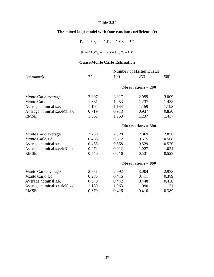
Table 2.29 The Mixed Logit Model With Four Random Coefficients (e)………………..……47

Table 2.30 The Mixed Logit Model With Four Random Coefficients (f)…..………………...…48

Table 2.31 The Mixed Logit Model With Four Random Coefficients (g)…………………....…49

Table 2.32 The Mixed Logit Model With Four Random Coefficients (h)…..………..…………50

Table 2.33 The Mixed Logit Model With Four Random Coefficients (i)……………….....……51

Table 2.34 The Mixed Logit Model With Four Random Coefficients (j)……………….....……52

Table 2.35 The Mixed Logit Model With Four Random Coefficients (k)………………………53

Table 2.36 The Mixed Logit Model With Four Random Coefficients (l)……………...…..……54

Table 2.37 The Mixed Logit Model With Four Random Coefficients (m)…………………...…55

Table 2.38 The Mixed Logit Model With Four Random Coefficients (n)………………..…..…56

Table 2.39 The Mixed Logit Model With Four Random Coefficients (o)………………………57

Table 2.40 The Mixed Logit Model With Four Random Coefficients (p)……………..……..…58

Table 3.1 90th

and 95th

Empirical Percentiles of Likelihood Ratio, Wald and Lagrange Multiplier

Test Statistical Distributions: One Random Parameter Model…………………………..65

Table 3.2 Rejection Rate of Likelihood Ratio, Wald and Lagrange Multiplier Test Statistic

Distributions: One Random Parameter Model..……………….........................................66

Table 3.3 Size Corrected Rejection Rates of LR, Wald and LM Test Statistic Distributions: One

Random Parameter Model............................................................................................….69

Table 3.4 90th

and 95th

Empirical Percentiles of Likelihood Ratio, Wald and Lagrange Multiplier

Test Statistical Distributions: Two Random Parameter Model………………………….72

Table 3.5 Rejection Rate of Likelihood Ratio, Wald and Lagrange Multiplier Test Statistic

Distributions: Two Random Parameter Model................................................................74

Table 3.6 Size Corrected Rejection Rates of LR, Wald and LM Test Statistic Distributions: Two

Random Parameter Model...............................................................……………………..76

vi

Table 4.1 The MSE of Uncorrelated RPL Model Estiamtes the MSE of Correlated RPL Model

Estimates………………………………..………………………………………………..91

Table 4.2 The t-test of the Average Relative Loss for the Pretest and Shrinkage

Estimators……………………………………………….…………………………….100

Table 4.3 The t-test of the Difference of the Average Relative Loss between the Pretest and

Shrinkage Estimators………..………………………………………………………….101

Table 4.4 The Fully Correlated Random Parameters Logit Model…………………………….104

Table 4.5 Parameter Estimates for the Fully Correlated Random Parameters Logit Model…...105

vii

LIST OF FIGURES

Figure 2.1 200 Points Generated by a Pseudo-Random Number Generator and the Halton

Sequence………............................................................................................................................11

Figure 2.2 Points of Two-Dimension Halton Sequence Generated with Prime 41 and 43……...12

Figure 3.1 Pretest Estimator RMSE Mixed Logit Estimator RMSE : One Random

Parameter Model…………………………………………………………………...…….62

Figure 3.2 The Rejection Rate of LR, Wald and LM Tests……………………..……………….67

Figure 3.3 The Size Corrected Rejection Rates: One Random Parameter Model……………….70

Figure 3.4 Pretest Estimation RMSE Mixed Logit Estimation RMSE : Two Random

Parameter Model.....................................……………..............................................…….71

Figure 3.5 The Rejection Rate of LR, Wald and LM Tests: Two Random Parameter Model......75

Figure 3.6 The Size Corrected Rejection Rates: Two Random Parameter Model….…………...77

Figure 4.1 The Ratios of LR, LM and Wald Based Pretest, Shrinkage Estimator MSE to the

Fully Correlated RPL Model Estimator MSE (estimated parameters mean)……………93

Figure 4.2 The Ratio of LR, LM and Wald Based Pretest, Shrinkage Estimator MSE to the

Fully Correlated RPL Model Estimator MSE (estimated variance of the coefficient

distribution)………………………………………………………………………………95


Fully Correlated RPL Model Estimator MSE (estimated parameters covariance)………96


Fully Correlated RPL Model Estimator MSE……………………………………………98

viii

ABSTRACT

This research uses quasi-Monte Carlo sampling experiments to examine the properties of

pretest and positive-part Stein-like estimators in the random parameters logit (RPL) model

based on the Lagrange Multiplier (LM), likelihood ratio (LR) and Wald tests. First, we

explore the properties of quasi-random numbers, which are generated by the Halton

sequence, in estimating the random parameters logit model. We show that increases in the

number of Halton draws influence the efficiency of the RPL model estimators only slightly.

The maximum simulated likelihood estimator is consistent and it is not necessary to increase

the number of Halton draws when the sample size increases for this result to be evident. In

the second essay, we study the power of the LM, LR and Wald tests for testing the random

coefficients in the RPL model, using the conditional logit model as the restricted model,

since we found that the LM-based pretest estimator provides the poor risk properties. We

claimed that the power of LR and Wald tests decreases with increases in the mean of the

coefficient distribution. The LM test has the weakest power for presence of the random

coefficient in the RPL model. In the last essay, the pretest and shrinkage are showed to

reduce the risk of the fully correlated RPL model estimators significantly. The percentage of

correct predicted choices is increased by 2% using the positive-part Stein-like estimates

compared to the results using the pretest and fully correlated RPL model estimates with using

the marketing consumer choice data.

1

CHAPTER 1 INTRODUCTION

The conditional logit model is frequently used in applied econometrics. The related

choice probability can be computed conveniently without multivariate integration. The

Independence from Irrelevant Alternatives (IIA) assumption of the conditional logit model is

inappropriate in many choice situations, especially for the choices that are close substitutes. The

IIA assumption arises because in logit models the unobserved components of utility are

independent and identically Type I extreme value distributions. This is violated in many cases,

such as when unobserved factors that affect the choice persist over time.

Unlike the conditional logit model, the random parameters logit (RPL) model, also called

the mixed logit model, does not impose the IIA assumption. The RPL model can capture random

taste variation among individuals and allows the unobserved factors of utility to be correlated

over time as well. However, the choice probability in the RPL model cannot be calculated

exactly because it involves a multi-dimensional integral which does not have closed form

solution. The integral can be approximated using simulation. The requirement of a large number

of pseudo-random numbers during the simulation leads to long computational times. In this

dissertation, we focus on the properties of pretest estimators and positive-part Stein-like

estimators in the random parameters logit model based on Lagrange multiplier (LM), likelihood

ratio (LR) and Wald test statistics. The outline of this dissertation as follows: in the second

chapter, we introduce quasi-random numbers and construct Monte Carlo experiments to explore

the properties of quasi-random numbers, which are generated by the Halton sequence, in

estimating the RPL model. In the third chapter, we use quasi-Monte Carlo sampling experiments

to examine the properties of pretest estimators in the RPL model based on the LM, LR and Wald

tests. The pretests are for the presence of random parameters. We explore the power of the LM,

2

LR and Wald tests for random parameters by calculating the empirical percentile values, size and

rejection rates of the test statistics, using the conditional logit model as the restricted model. In

the fourth chapter, the number of random coefficients in the random parameters logit model is

extended to four and allowed to be correlated to each other. We explore the properties of pretest

estimators and positive-part Stein-like estimators which are a stochastically weighted convex

combination of fully correlated parameter model estimators and uncorrelated parameter model

estimators in the random parameters logit (RPL) model. The mean squared error (MSE) is used

as the risk criterion to compare the efficiency of positive part Stein-like estimators to the

efficiency of pretest and fully correlated RPL model estimators, which are based on the

likelihood ratio (LR), Lagrange multiplier (LM) and Wald test statistics. Lastly, the accuracy of

correct predicted choices is calculated and compared with the positive-part Stein-like, pretest and

fully correlated RPL model estimators using marketing consumer choice data.

3

CHAPTER 2 USING HALTON SEQUENCES IN THE RANDOM

PARAMETERS LOGIT MODEL

2.1 Introduction

In this chapter, we construct Monte Carlo experiments to explore the properties of quasi-

random numbers, which are generated by the Halton sequence, in estimating the random

parameters logit (RPL) model. The random parameters logit model has become more frequently

used in applied econometrics because of its high flexibility. Unlike the multinomial logit model

(MNL), this model is not limited by the Independence from Irrelevant Alternatives (IIA)

assumption. It can capture the random preference variation among individuals and allows

unobserved factors of utility to be correlated over time. The choice probability in the RPL model

cannot be calculated exactly because it involves a multi-dimensional integral which does not

have closed form. The use of pseudo-random numbers to approximate the integral during the

simulation requires a large number of draws and leads to long computational times.

To reduce the computational cost, it is possible to replace the pseudo-random numbers by

a set of fewer, evenly spaced points and still achieve the same, or even higher, estimation

accuracy. Quasi-random numbers are evenly spread over the integration domain. They have

become popular alternatives to pseudo-random numbers in maximum simulated likelihood

problems. Bhat (2001) compared the performance of quasi-random numbers (Halton draws) and

pseudo-random numbers in the context of the maximum simulated likelihood estimation of the

RPL model. He found that using 100 Halton draws the root mean squared error (RMSE) of the

RPL model estimates were smaller than using 1000 pseudo-random numbers. However, Bhat

also mentioned that the error measures of the estimated parameters do not always become

smaller as the number of Halton draws increases. Train (2003, p. 234) summarizes some

numerical experiments comparing the use of 100 Halton draws with 125 Halton draws. He says,

4

“…the standard deviations were greater with 125 Halton draws than with 100 Halton draws….”

Its occurrence indicates the need for further investigation of the properties of Halton sequences

in simulation-based estimation.” It is our purpose to further the understanding of these properties

through extensive simulation experiments. How does the number of quasi-random numbers,

which are generated by the Halton draws, influence the efficiency of the estimated parameters?

How should we choose the number of Halton draws in the application of Halton sequences with

the maximum simulated likelihood estimation? In our experiments, we vary the number of

Halton draws, the sample size and the number of random coefficients to explore the properties of

the Halton sequences in estimating the RPL model. The results of our experiments confirm the

efficiency of the quasi-random numbers in the context of the RPL model. We show that increases

in the number of Halton draws influence the efficiency of the random parameters logit model

estimators by a small amount. The maximum simulated likelihood estimator is consistent. In the

context of the RPL model, we find that it is not necessary to increase the number of Halton

draws when the sample size increases for this result to be evident.

The plan of the remainder of the first chapter is as follows. In the following section, we

discuss the random parameters logit specification. Section 2.3 introduces the Halton sequence.

Section 2.4 describes our Monte Carlo experiments. Section 2.5 presents the experimental

results. Some conclusions are given in Section 2.6.

2. 2 The Random Parameters Logit Model

The random parameters logit model, also called the mixed logit model, was first applied

by Boyd and Mellman (1980) and Cardell and Dunbar (1980) to forecast automobile choices by

individuals. As its name implies, the RPL model allows the coefficients to be random to capture

the preferences of individuals. It relaxes the IIA assumption, that the ratio of probabilities of two

alternatives is not affected by the number of other alternatives. The random parts of the utility in

5

the RPL model can be decomposed into two parts: one part having the independent, identical

type I extreme value distribution, and the other, representing individual tastes, can be any

distribution. The related utility associated with alternative i as evaluated by individual n in the

RPL model is written as:

(2.1) '

ni n ni niU x

where nix are observed variables for alternative i and individual n ,

n is a vector of coefficients

for individual n varying over individuals in the population with density function ( )f , and ni is

iid extreme value, which is independent of n and

nix . The distribution of coefficient n is

specified by researchers. David A. Hensher and Willian H. Greene (2003) discussed how to

choose an appropriate distribution for random coefficients. Here, the random coefficients n can

be separated into their mean and random component nv .

(2.2) ni ni n ni niU x v x

Even if the elements of nv are uncorrelated, the random parts of utility

ni , where ,ni n ni niv x

in the RPL model are still correlated over the alternatives. The variance of the random

component can be different for different individuals. The RPL model becomes the probit model,

if ni has a multivariate normal distribution. If

n is fixed, the RPL model becomes the standard

logit model:

(2.3) ni ni niU x

The probability that the individual n choose alternative i is:

(2.4) ( ) ( ) ( )ni ni nj ni ni nj nj nj ni ni njP P U U i j P x x i j P x x i j

6

Marschak is the first person that provided the nonconstructive proof to show that the Type I

extreme value distribution of random part of utility ni can lead to logistic distribution of the

difference between two random terms ( )ni nj . The proof was developed by E. Holman and A.

Marley and completed by Daniel McFadden (1974). So the choice probability niP of conditional

logit model has a succinct and closed form:

(2.5) ( )ni

nj

x

ni ni x

j

eP L

e

Since n is random and unobserved in the RPL model, the choice probability

niP cannot be

calculated as it is in the standard logit model. It must be evaluated at different values of n and

the form of the related choice probability is:

(2.6) ( )ni

nj

x

ni nix

j

eP f d E L

e

The density function ( )f provides the weights, and the choice probability is a weighted average

of ( )niL over all possible values ofn . Even though the integral in (2.6) does not have a closed

form, the choice probability in the RPL model can be estimated through simulation. The

unknown parameters ( ) , such as the mean and variance of the random coefficient distribution,

can be estimated by maximizing the simulated log-likelihood function. With simulation, a value

of labeled as r representing the rth draw, is selected randomly from a previously specified

distribution. The standard logit ( )niL in equation (2.6) can be calculated with r . Repeating

this process R times, the simulated probability of individual n choosing alternative i is obtained

by averaging ( )r

niL :

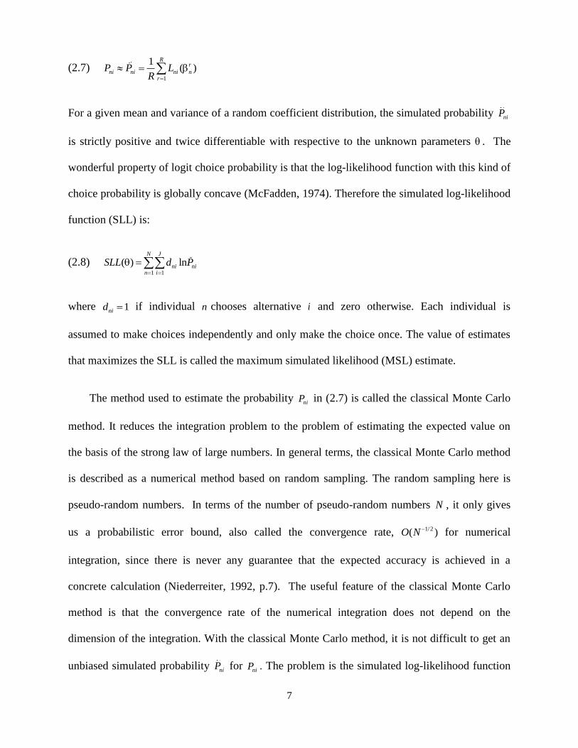
7

(2.7) 1

1( )

Rr

ni ni ni nr

P P LR

For a given mean and variance of a random coefficient distribution, the simulated probability niP

is strictly positive and twice differentiable with respective to the unknown parameters . The

wonderful property of logit choice probability is that the log-likelihood function with this kind of

choice probability is globally concave (McFadden, 1974). Therefore the simulated log-likelihood

function (SLL) is:

(2.8) 1 1

( ) lnN J

ni nin i

SLL d P

where 1nid if individual n chooses alternative i and zero otherwise. Each individual is

assumed to make choices independently and only make the choice once. The value of estimates

that maximizes the SLL is called the maximum simulated likelihood (MSL) estimate.

The method used to estimate the probability niP in (2.7) is called the classical Monte Carlo

method. It reduces the integration problem to the problem of estimating the expected value on

the basis of the strong law of large numbers. In general terms, the classical Monte Carlo method

is described as a numerical method based on random sampling. The random sampling here is

pseudo-random numbers. In terms of the number of pseudo-random numbers N , it only gives

us a probabilistic error bound, also called the convergence rate, 1/2( )O N for numerical

integration, since there is never any guarantee that the expected accuracy is achieved in a

concrete calculation (Niederreiter, 1992, p.7). The useful feature of the classical Monte Carlo

method is that the convergence rate of the numerical integration does not depend on the

dimension of the integration. With the classical Monte Carlo method, it is not difficult to get an

unbiased simulated probability niP for niP . The problem is the simulated log-likelihood function

8

in (2.8) is a logarithmic transformation, which causes a simulation bias in the SLL which

translates into bias in the MSL estimator. To decrease the bias in the MSL estimator and get a

consistent and efficient MSL estimator, Train (2003, p.257) shows that, with an increase in the

sample size N , the number of pseudo-random numbers should rise faster than N . The

disadvantage of the classical Monte Carlo method in the RPL model estimation is the

requirement of a large number of pseudo-random numbers, which leads to long computational

times.

2.3 The Halton Sequences

To reduce the computational cost, quasi-random numbers are being used to replace the

pseudo-random numbers in MSL estimation, leading to the same or even higher accuracy

estimation with many fewer points. The essence of the number theoretic method (NTM) is to

find a set of uniformly scattered points over an s -dimensional unit cube. Such set of points

obtained by NTM is usually called a set of quasi-random numbers, or a number theoretic net.

Sometimes it can be used in the classical Monte Carlo method to achieve a significantly higher

accuracy. The Monte Carlo method with using quasi-random numbers is called a quasi-Monte

Carlo method. In fact, there are several classical methods to construct the quasi-random numbers.

Here we use the Halton sequences proposed by Halton (1960).

The Halton sequences are based on the base- p number system which implies that any

integer n can be written as:

(2.9) 2

1 2 1 0 0 1 2

M

M M Mn n n n n n n n p n p n p

where [log ] [ln / ln ]n

pM n p and 1M is called the number of digits of n , square brackets

denoting the integral part, p is base and can be any integer except 1, in is the digit at position i ,

9

0 i M , 0 1in p and ip is the weight of position i . For example, with the base 10p , the

integer 468n has 0 1 28, 6, 4n n n .

Using the base- p number system, we can construct one and only one fraction which is

smaller than 1 by writing n with a different base number system and reversing the order of the

digits in n . It is also called the radical inverse function defined as the follows:

(2.10) 1 2 1

0 1 2 0 1( ) 0. M

p M Mn n n n n n p n p n p

Based on the base- p number system, the integer 468n can be converted into the binary

number system by successively dividing by the new base 2:

10468 8 7 6 5 4 3 2 1 0

21 2 1 2 1 2 0 2 1 2 0 2 1 2 0 2 0 2 111010100

Applying the radical inverse function, we can get an unique fraction for the integer 468n with

base 2p :

3 5 7 8 9

2 2 10(111010100) 0.001010111 1 2 1 2 1 2 1 2 1 2 0.169921875

The value 100.169921875 is the corresponding fraction of

20.001010111 in the decimal number

system.

The Halton sequence of length N is developed from the radical inverse function and the

points of the Halton sequence are ( )p n for 1,2n N , where p is a prime number. The k -

dimensional sequence is defined as:

(2.11) 1 2

( ( ), ( ), ( ))kn p p pn n n

10

Where 1 2, , kp p p

are prime to each other and are chosen from the first k primes. By setting

1 2, , kp p p to be prime to each other we avoid the correlation among the points generated by any

two Halton sequences with different base- p .

In applications, Halton sequences are used to replace random number generators to

produce points in the interval [0, 1]. The points of the Halton sequence are generated iteratively.

As far as a one-dimensional Halton sequence is concerned, the Halton sequence based on prime

p divides the 0-1 space into p segments and systematically fills in the empty space by dividing

each segment into smaller p segments iteratively. This is illustrated below. The numbers below

the line represents the order of points filling in the space.

0 1/8 ¼ 3/8 1/2 5/8 ¾ 7/8 1

| | | | | | | | |

4 2 6 1 5 3 7

The position of the points is determined by the base which is used to construct the iteration. A

large base implies more points in each iteration or long cycle. Due to the high correlation among

the initial points of the Halton sequence, the first ten points of the sequences are usually

discarded in applications (Train, 2003, p.230). Compared to the pseudo-random numbers, the

coverage of the points of the Halton sequence are more uniform, since the pseudo-random

numbers may cluster in some areas and leave some areas uncovered. This can be seen from

Figure 1, which is similar to the graph in Fang and Wang (1994). In Figure 2.1, the top one is a

plot of 200 points taken from uniform distribution of two dimensions using pseudo-random

numbers. The bottom one is a plot of 200 points obtained by the Halton sequence. The latter

scatters more uniformly on the unit square than the former. Since the points generated from the

Halton sequences are deterministic points, unlike the classical-Monte Carlo method, quasi-Monte

11

Carlo provides a deterministic error bound instead of probabilistic error bound. It is also called

the discrepancy in the literature of number theoretic methods. The smaller the discrepancy, the

more evenly the quasi-random numbers are spread over the domain. The deterministic error

bound of quasi-Monte Carlo method with the k -dimensional Halton sequence is 1( (ln ) )kO N N ,

which represented in terms of the number of points used and shown smaller than the probabilistic

error bound of classical-Monte Carlo method [refer to Appendix A]. For example, as shown in

Appendix A, if we increase the length of the Halton sequence from N to N and let 2N N , the

discrepancy is 2( (2ln ) )kO N N . This implies that, unlike the pseudo-random numbers, the

increases in the number of points generated by the Halton sequence can’t surely improve the

discrepancy, especially for the high dimensional Halton sequence. In applications, Bhat (2001),

Train (2003), Hess and Polak (2003) and other researchers discussed this issue by showing the

high correlation among the points generated by the Halton sequences with any two adjacent

prime numbers.

Figure 2.1 200 points generated by a pseudo-random number Generator and the Halton Sequence

12

With high dimensional Halton sequences, usually 10k , a large number of points is

needed to complete the long cycle with large prime numbers. In addition to increasing the

computational time, it will also cause a correlation between two adjacent large prime-based

sequences, such as the thirteenth and fourteenth dimension generated by prime number 41 and 43

respectively. The correlation coefficient between two close large prime-based sequences is

almost equal to one. This is shown in Figure 2.2, which is based on a graph from Bhat (2003). To

solve this problem, number theorists such as Wang and Hickernell (2000) scramble the digits of

each number of the sequences, which is called a scrambled Halton sequences. Bhat (2003) shows

that the scrambled Halton sequence performs better than the standard Halton sequence, or the

pseudo-random sequence, in estimating the mixed probit model with a 10-dimensional integral.

In this chapter, we analyze the properties of the Halton sequence when estimating the RPL model

with a low dimensional integral. In the next section we will describe our experiments and find

the answers to the above questions.

Figure 2.2: 200 points of two-dimension Halton sequence generated with prime 41 and 43

13

2.4 The Quasi-Monte Carlo Experiments with Halton Sequences

Our experiments begin from the simple RPL model which has no intercept term and

only one random coefficient. Then, we expand the number of random coefficient to four by

adding the random coefficient one by one. In our experiments, each individual faces four

mutually exclusive alternatives with only one choice occasion. The associated utility for

individual n choosing alternative i is:

(2.12) ni n ni niU x

The explanatory variables for each individual and each alternative nix are generated from

independent standard normal distributions. The coefficients for each individual n are generated

from normal distribution 2( , )N . These values of nix and

n are held fixed over each

experiment design. The choice probability for each individual is generated by comparing the

utility of each alternative:

(2.13) 1

0

r r

r n ni ni n nj nj

ni

x xI

Otherwise

i j

The indicator function r

niI represents whether individual n chooses alternative i or not based on

the utility function. The values of errors are generated from iid extreme value type I distribution,

r

ni representing the rth draw. We calculate and compare the utility of each alternative using these

values of errors. This process is repeated 1000 times. The choice probability niP for each

individual n choosing alternative i is:

(2.14) 1000

1

1

1000

r

ni nir

P I

14

The dependent variables niy are determined by these values of simulated choice probabilities.

Our generated data are composed of the explanatory and dependent variables nix and

niy which

are used to estimate the RPL model parameters. In our experiments, we generate 999 Monte

Carlo samples ( )NSAM with specific true values that we set for the RPL model parameters. The

reason that we generate 999 Monte Carlo samples is that it will be convenient to calculate the

empirical 90th

and 95th

percentile value of the LR, Wald and LM statistics in the following

chapter. During the estimation process, the random coefficients

n in (2.7) are generated by the

Halton sequences instead of pseudo-random numbers. First, we generate the k-dimensional

Halton sequences of length 10N R , where N is sample size, R is the number of the Halton

draws assigned to each individual and 10 is the number of Halton draws that we discard due to

the high correlation [Morokoff and Caflisch (1995), Bratley, et al. (1992)]. Then we transform

these Halton draws into a set of numbers n with normal distribution using the inverse transform

method. With the inverse transform method, the random variables have independent multivariate

normal distribution n which are transformed from the k -dimensional Halton sequences, have

the same discrepancy as the Halton sequences generated from the k -dimensional unit cube. So

the smaller discrepancy of the Halton sequences leads to the smaller discrepancy of n . To

calculate the corresponding simulated probability niP in (2.7), the first R points are assigned to

the first individual, the second R points are used to calculate the simulated probability niP of the

second individual, and so on.

To examine the efficiency of the estimated parameters using Halton sequences, the root

mean squared error (RMSE) of the RPL model estimates is used as the error measure. And we

also compare the average nominal standard errors to the Monte Carlo standard deviations of the

15

estimated parameters, which are regarded as the true standard deviations of estimated

parameters. They are calculated as follows using one parameter as an example:

MC average1

ˆ ˆ /NSAM

ii

NSAM

MC standard deviation (s.d.) of =2

1

ˆ ˆ( ) ( 1)NSAM

ii

NSAM

Average nominal standard error (s.e.) of =1

ˆvar( )NSAM

ii

NSAM

Root mean square error (RMSE) of = 2

1

ˆ( )NSAM

ii

NSAM

where and ˆi

are the true parameter and estimates of the parameter, respectively. To explore

the properties of the Halton sequences in estimating the RPL model, we vary the number of

Halton draws, the sample size and the number of random coefficients. We also do the same

experiments using the pseudo-random numbers to compare the performance of the Halton

sequence and pseudo-random numbers in estimating the RPL model. To avoid different

simulation errors from the different process of probability integral transformation, we use the

same probability integral transformation method (CDFNI procedure, see Gauss help manual)

with Halton draws and pseudo-random numbers.

2.5 The Experimental Results

In our experiments, we increase the number of random coefficients one by one. For each

case, the RPL model is estimated using 25, 100, 250 and 500 Halton draws. We use 2000

pseudo-random numbers to get the benchmark results which are used as the “true” results to

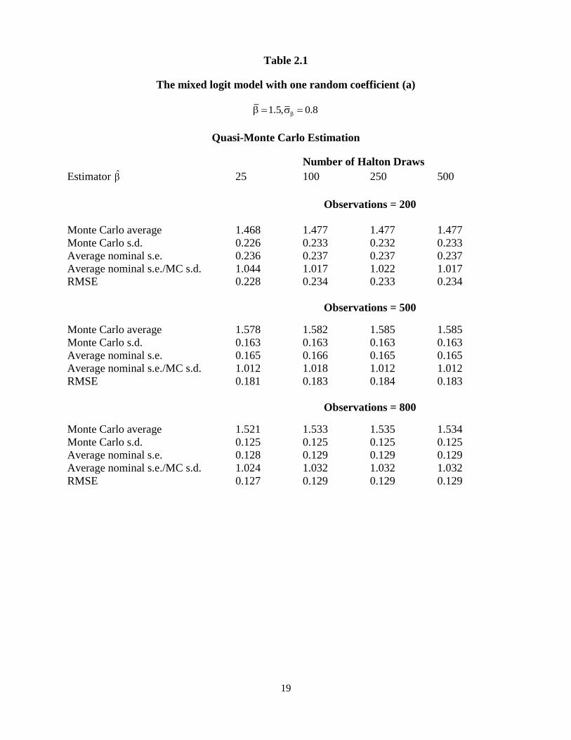
compare the others. Table 2.1 and Table 2.2 show the results of the one random coefficient

parameter logit model using Halton draws. Tables 2.3 and 2.4 present the results using 1000 and

2000 pseudo-random numbers. From Table 2.1 and Table 2.2, for the given number of

16

observations, increasing the number of Halton draws from 25 to 500 only changes the RMSE of

the estimated mean of the random coefficient distribution by less than 3%, and influences the

RMSE of the estimated standard deviation of the random coefficient distribution by no more than

8%. With increases in the number of Halton draws, the RMSE of the estimated parameters does

not always decline. It is also true for the pseudo-random numbers. With the given number of

observations, the percentage change of the RMSE of estimated parameters is less than 2.5% with

increases in the number of pseudo-random numbers. The RMSE of and ˆ using 500 Halton

draws is closer to the benchmark results than that using 25 Halton draws. However, the RMSE

of the estimated mean of the random coefficient is lower using 25 Halton draws than it using

1000 pseudo-random numbers. With 100 Halton draws, we can reach almost the same efficiency

of the RPL model estimators as using 2000 pseudo-random numbers. The results are consistent

with Bhat (2001). The ratios of the average nominal standard errors of estimated parameters to

the Monte Carlo standard deviations of estimated parameters are stable with increases in the

number of Halton draws. At the same time, for the given number of Halton draws, increasing the

number of observations decreases the RMSE of the RPL estimators.

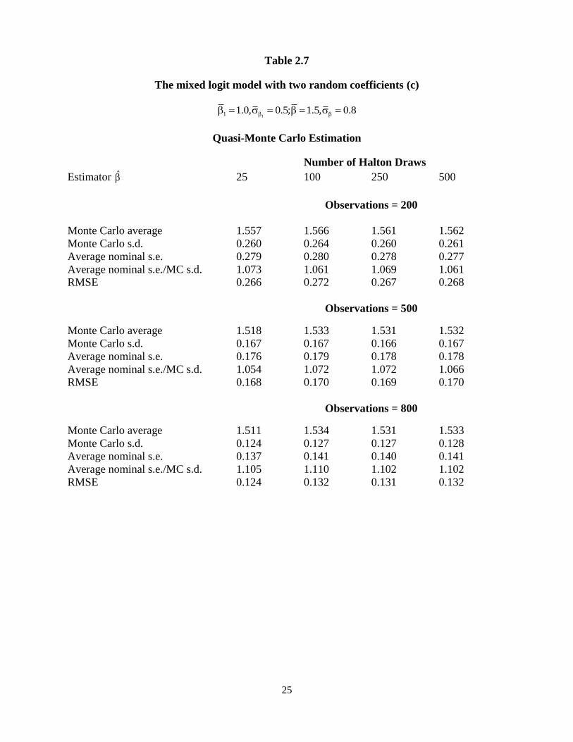
Tables 2.5-2.12 present the results of two independent random coefficients logit model

using Halton draws and pseudo-random numbers. We set the mean and the standard deviation of

the new random coefficient as 1.0 and 0.5 respectively. Because the larger ratio of the parameter

mean to its standard deviation makes the simulated likelihood function flatter and leads estimates

hard to converge to the maximum value, the value of the ratio is controlled around 2. We use the

same error measures to explore the efficiency of each estimator for each case. After including

another random coefficient, the mean of each random coefficient is overestimated by 3%. The

RMSE of the RPL estimator is stable in the number of Halton draws. However, the RMSE of the

RPL estimator using 500 Halton draws is not always closer to the benchmark results than those

17

using 25 Halton draws. This phenomenon happens more frequently with the increases in the

number of random coefficients. For a given number of Halton draws, the RMSE of the RPL

model estimator decreases in the number of observations.

With the increases in the number of random coefficients, the computational time

increases greatly using pseudo-random numbers rather than using quasi-random numbers.

Tables 2.13-2.40 show the results of three and four independent random coefficients logit

models. The results are similar to the one and two random coefficients cases. Train (2003, p.

228) discusses that the negative correlation between the average of two adjacent observation’s

draws can reduce errors in the simulated log-likelihood function, like the method of antithetic

variates. However, this negative covariance across observations declines with in the number of

observations, since the length of Halton sequences in estimating the RPL model is determined by

the number of observations N and the number of Halton draws R assigned to each observation

and the increases in N will decrease the gap between two adjacent observation’s coverage. So

Train (2003, p.228) suggests increasing the number of Halton draws for each individual when the

number of observations increases. But, based on our experimental results with low dimensions,

we find that, with increases in the number of observations, increasing the number of Halton

draws for each individual does not improve the efficiency of the RPL model.

2.6 Conclusions

In this paper we study the properties of the Halton sequences in estimating the RPL

model with one to four independent random coefficients. The increases in the number of points

generated by the Halton sequence can’t surely improve the discrepancy, especially for the high

dimensional Halton sequence. For low dimensional integrals the theoretical discrepancy for

Halton sequences in estimating the k -dimensional integrals decreases in the length of the Halton

sequences. With low dimensional integrals, we expected the improvement in the efficiency of

18

the RPL model estimators by increasing the number of Halton draws for each individual,

especially when there is an increase in the number of observations. However, there is no

evidence in any of our experiments to show that the increases in the number of Halton draws can

significantly influence the efficiency of the RPL model estimators. The efficiency of the RPL

model estimator is stable in the number of Halton draws. It implies that it is not necessary to

increase the number of Halton draws with increases in the number of observations. In our

experiments, using 25 Halton draws can achieve the same estimator efficiency as using 1000

pseudo-random numbers. This result doesn’t change by increasing the number of observations.

These results are also true for the correlated random coefficients cases, since the correlated

distribution can be transformed into independent one by using the Cholesky decomposition.

19

Table 2.1

The mixed logit model with one random coefficient (a)

1.5, 0.8

Quasi-Monte Carlo Estimation

Number of Halton Draws

Estimator 25 100 250 500

Observations = 200

Monte Carlo average 1.468 1.477 1.477 1.477

Monte Carlo s.d. 0.226 0.233 0.232 0.233

Average nominal s.e. 0.236 0.237 0.237 0.237

Average nominal s.e./MC s.d. 1.044 1.017 1.022 1.017

RMSE 0.228 0.234 0.233 0.234

Observations = 500


Monte Carlo s.d. 0.163 0.163 0.163 0.163



RMSE 0.181 0.183 0.184 0.183

Observations = 800


Monte Carlo s.d. 0.125 0.125 0.125 0.125



RMSE 0.127 0.129 0.129 0.129

20

Table 2.2

The mixed logit model with one random coefficient (b)

1.5, 0.8



Estimator ˆ 25 100 250 500

Observations = 200


Monte Carlo s.d. 0.337 0.372 0.375 0.377



RMSE 0.395 0.419 0.424 0.426

Observations = 500


Monte Carlo s.d. 0.236 0.243 0.242 0.243



RMSE 0.246 0.250 0.249 0.250

Observations = 800


Monte Carlo s.d. 0.177 0.173 0.172 0.172



RMSE 0.187 0.177 0.176 0.176

21

Table 2.3

The mixed logit model with one random coefficient (c)

1.5, 0.8

Classical-Monte Carlo Estimation

Number of Random Draws

Estimator 1000 2000

Observations = 200

Monte Carlo average 1.479 1.483

Monte Carlo s.d. 0.229 0.233

Average nominal s.e. 0.236 0.239

Average nominal s.e./MC s.d. 1.031 1.026

RMSE 0.230 0.234

Observations = 500





RMSE 0.182 0.187

Observations = 800





RMSE 0.128 0.130

22

Table 2.4

The mixed logit model with one random coefficient (d)

1.5, 0.8



Estimator ˆ 1000 2000

Observations = 200





RMSE 0.400 0.410

Observations = 500





RMSE 0.242 0.245

Observations = 800





RMSE 0.177 0.175

23

Table 2.5

The mixed logit model with two random coefficients (a)

11 1.0, 0.5; 1.5, 0.8



Estimator 1 25 100 250 500

Observations = 200


Monte Carlo s.d. 0.168 0.176 0.174 0.175



RMSE 0.168 0.176 0.174 0.175

Observations = 500


Monte Carlo s.d. 0.107 0.111 0.111 0.111



RMSE 0.108 0.115 0.115 0.115

Observations = 800


Monte Carlo s.d. 0.083 0.086 0.086 0.086



RMSE 0.083 0.089 0.088 0.089

24

Table 2.6

The mixed logit model with two random coefficients (b)

11 1.0, 0.5; 1.5, 0.8



Estimator 1

ˆ 25 100 250 500

Observations = 200


Monte Carlo s.d. 0.315 0.350 0.358 0.358



RMSE 0.322 0.357 0.369 0.368

Observations = 500


Monte Carlo s.d. 0.221 0.229 0.230 0.230



RMSE 0.222 0.229 0.230 0.230

Observations = 800


Monte Carlo s.d. 0.184 0.191 0.194 0.196



RMSE 0.189 0.192 0.196 0.197

25

Table 2.7

The mixed logit model with two random coefficients (c)

11 1.0, 0.5; 1.5, 0.8



Estimator 25 100 250 500

Observations = 200


Monte Carlo s.d. 0.260 0.264 0.260 0.261



RMSE 0.266 0.272 0.267 0.268

Observations = 500


Monte Carlo s.d. 0.167 0.167 0.166 0.167



RMSE 0.168 0.170 0.169 0.170

Observations = 800


Monte Carlo s.d. 0.124 0.127 0.127 0.128



RMSE 0.124 0.132 0.131 0.132

26

Table 2.8

The mixed logit model with two random coefficients (d)

11 1.0, 0.5; 1.5, 0.8



Estimator ˆ 25 100 250 500

Observations = 200


Monte Carlo s.d. 0.338 0.330 0.326 0.328



RMSE 0.345 0.343 0.336 0.338

Observations = 500


Monte Carlo s.d. 0.221 0.212 0.213 0.213



RMSE 0.222 0.216 0.215 0.216

Observations = 800


Monte Carlo s.d. 0.163 0.161 0.161 0.161



RMSE 0.165 0.161 0.161 0.161

27

Table 2.9

The mixed logit model with two random coefficients (e)

11 1.0, 0.5; 1.5, 0.8



Estimator 1 1000 2000

Observations = 200





RMSE 0.173 0.176

Observations = 500





RMSE 0.113 0.116

Observations = 800





RMSE 0.086 0.089

28

Table 2.10

The mixed logit model with two random coefficients (f)

11 1.0, 0.5; 1.5, 0.8



Estimator 1

ˆ 1000 2000

Observations = 200





RMSE 0.341 0.350

Observations = 500





RMSE 0.219 0.221

Observations = 800





RMSE 0.189 0.188

29

Table 2.11

The mixed logit model with two random coefficients (g)

11 1.0, 0.5; 1.5, 0.8



Estimator 1000 2000

Observations = 200





RMSE 0.266 0.268

Observations = 500





RMSE 0.168 0.169

Observations = 800





RMSE 0.130 0.131

30

Table 2.12

The mixed logit model with two random coefficients (h)

11 1.0, 0.5; 1.5, 0.8




Observations = 200





RMSE 0.326 0.338

Observations = 500





RMSE 0.210 0.218

Observations = 800





RMSE 0.158 0.162

31

Table 2.13

The mixed logit model with three random coefficients (a)

1 21 21.0, 0.5; 2.5, 1.2; 1.5, 0.8



Estimator 1 25 100 250 500

Observations = 200


Monte Carlo s.d. 0.230 0.222 0.285 0.228


Average nominal s.e./MC s.d . 1.083 1.113 0.905 1.083

RMSE 0.230 0.222 0.285 0.228

Observations = 500


Monte Carlo s.d. 0.142 0.157 0.161 0.158



RMSE 0.142 0.159 0.166 0.161

Observations = 800


Monte Carlo s.d. 0.109 0.126 0.128 0.126



RMSE 0.113 0.146 0.152 0.150

32

Table 2.14

The mixed logit model with three random coefficients (b)

1 21 21.0, 0.5; 2.5, 1.2; 1.5, 0.8



Estimator1

ˆ 25 100 250 500

Observations = 200


Monte Carlo s.d. 0.355 0.346 0.401 0.350



RMSE 0.470 0.462 0.508 0.464

Observations = 500


Monte Carlo s.d. 0.197 0.227 0.237 0.234



RMSE 0.228 0.280 0.293 0.282

Observations = 800


Monte Carlo s.d. 0.181 0.197 0.200 0.198



RMSE 0.214 0.259 0.265 0.259

33

Table 2.15

The mixed logit model with three random coefficients (c)

1 21 21.0, 0.5; 2.5, 1.2; 1.5, 0.8



Estimator2 25 100 250 500

Observations = 200


Monte Carlo s.d. 0.477 0.438 0.657 0.467



RMSE 0.496 0.473 0.674 0.498

Observations = 500


Monte Carlo s.d. 0.331 0.347 0.354 0.347



RMSE 0.345 0.353 0.355 0.350

Observations = 800


Monte Carlo s.d. 0.241 0.265 0.271 0.267



RMSE 0.271 0.271 0.273 0.269

34

Table 2.16

The mixed logit model with three random coefficients (d)

1 21 21.0, 0.5; 2.5, 1.2; 1.5, 0.8



Estimator2

ˆ 25 100 250 500

Observations = 200


Monte Carlo s.d. 0.497 0.454 0.573 0.484



RMSE 0.573 0.574 0.661 0.600

Observations = 500


Monte Carlo s.d. 0.352 0.339 0.317 0.317



RMSE 0.375 0.366 0.337 0.343

Observations = 800


Monte Carlo s.d. 0.251 0.246 0.236 0.232



RMSE 0.272 0.259 0.245 0.242

35

Table 2.17

The mixed logit model with three random coefficients (e)

1 21 21.0, 0.5; 2.5, 1.2; 1.5, 0.8



Estimator 25 100 250 500

Observations = 200


Monte Carlo s.d. 0.296 0.266 0.377 0.289



RMSE 0.314 0.294 0.393 0.314

Observations = 500


Monte Carlo s.d. 0.200 0.215 0.221 0.215



RMSE 0.204 0.215 0.221 0.215

Observations = 800


Monte Carlo s.d. 0.160 0.178 0.182 0.179



RMSE 0.163 0.194 0.204 0.201

36

Table 2.18

The mixed logit model with three random coefficients (f)

1 21 21.0, 0.5; 2.5, 1.2; 1.5, 0.8



Estimator ˆ 25 100 250 500

Observations = 200


Monte Carlo s.d. 0.327 0.320 0.404 0.369



RMSE 0.561 0.587 0.647 0.638

Observations = 500


Monte Carlo s.d. 0.306 0.322 0.330 0.329



RMSE 0.333 0.333 0.338 0.340

Observations = 800


Monte Carlo s.d. 0.235 0.250 0.247 0.249



RMSE 0.266 0.255 0.251 0.252

37

Table 2.19

The mixed logit model with three random coefficients (g)

1 21 21.0, 0.5; 2.5, 1.2; 1.5, 0.8




Observations = 200





RMSE 0.231 0.237

Observations = 500





RMSE 0.158 0.164

Observations = 800





RMSE 0.144 0.154

38

Table 2.20

The mixed logit model with three random coefficients (h)

1 21 21.0, 0.5; 2.5, 1.2; 1.5, 0.8



Estimator 1

ˆ 1000 2000

Observations = 200





RMSE 0.465 0.473

Observations = 500





RMSE 0.274 0.282

Observations = 800





RMSE 0.247 0.258

39

Table 2.21

The mixed logit model with three random coefficients (i)

1 21 21.0, 0.5; 2.5, 1.2; 1.5, 0.8




Observations = 200





RMSE 0.507 0.513

Observations = 500





RMSE 0.344 0.348

Observations = 800





RMSE 0.270 0.268

40

Table 2.22

The mixed logit model with three random coefficients (j)

1 21 21.0, 0.5; 2.5, 1.2; 1.5, 0.8



Estimator 2

ˆ 1000 2000

Observations = 200





RMSE 0.589 0.592

Observations = 500





RMSE 0.331 0.342

Observations = 800





RMSE 0.246 0.246

41

Table 2.23

The mixed logit model with three random coefficients (k)

1 21 21.0, 0.5; 2.5, 1.2; 1.5, 0.8



Estimator 1000 2000

Observations = 200





RMSE 0.323 0.327

Observations = 500





RMSE 0.213 0.214

Observations = 800





RMSE 0.197 0.201

42

Table 2.24

The mixed logit model with three random coefficients (l)

1 21 21.0, 0.5; 2.5, 1.2; 1.5, 0.8




Observations = 200





RMSE 0.609 0.585

Observations = 500





RMSE 0.336 0.325

Observations = 800





RMSE 0.252 0.245

43

Table 2.25

The mixed logit model with four random coefficients (a)

1 21 21.0, 0.5; 2.5, 1.2

33 3.0, 1.5; 1.5, 0.8



Estimator 1 25 100 250 500

Observations = 200


Monte Carlo s.d. 0.667 0.460 0.458 0.495



RMSE 0.687 0.472 0.469 0.505

Observations = 500


Monte Carlo s.d. 0.168 0.212 0.183 0.182



RMSE 0.190 0.214 0.189 0.189

Observations = 800


Monte Carlo s.d. 0.107 0.146 0.146 0.141



RMSE 0.171 0.156 0.155 0.152

44

Table 2.26

The mixed logit model with four random coefficients (b)

1 21 21.0, 0.5; 2.5, 1.2

33 3.0, 1.5; 1.5, 0.8



Estimator1

ˆ 25 100 250 500

Observations = 200


Monte Carlo s.d. 0.576 0.427 0.423 0.448



RMSE 0.580 0.461 0.469 0.485

Observations = 500


Monte Carlo s.d. 0.301 0.326 0.314 0.314



RMSE 0.303 0.326 0.316 0.315

Observations = 800


Monte Carlo s.d. 0.208 0.278 0.278 0.273



RMSE 0.234 0.278 0.278 0.273

45

Table 2.27

The mixed logit model with four random coefficients (c)

1 21 21.0, 0.5; 2.5, 1.2

33 3.0, 1.5; 1.5, 0.8



Estimator2 25 100 250 500

Observations = 200


Monte Carlo s.d. 1.530 1.099 1.106 1.255



RMSE 1.547 1.104 1.110 1.259

Observations = 500


Monte Carlo s.d. 0.356 0.461 0.391 0.389



RMSE 0.547 0.543 0.512 0.515

Observations = 800


Monte Carlo s.d. 0.224 0.327 0.321 0.304



RMSE 0.459 0.396 0.385 0.381

46

Table 2.28

The mixed logit model with four random coefficients (d)

1 21 21.0, 0.5; 2.5, 1.2

33 3.0, 1.5; 1.5, 0.8



Estimator2

ˆ 25 100 250 500

Observations = 200


Monte Carlo s.d. 1.203 0.944 0.901 1.020



RMSE 1.214 0.947 0.903 1.022

Observations = 500


Monte Carlo s.d. 0.360 0.412 0.384 0.378



RMSE 0.511 0.494 0.483 0.484

Observations = 800


Monte Carlo s.d. 0.246 0.313 0.298 0.289



RMSE 0.380 0.355 0.335 0.335

47

Table 2.29

The mixed logit model with four random coefficients (e)

1 21 21.0, 0.5; 2.5, 1.2

33 3.0, 1.5; 1.5, 0.8



Estimator3 25 100 250 500

Observations = 200


Monte Carlo s.d. 1.661 1.253 1.237 1.438



RMSE 1.663 1.253 1.237 1.437

Observations = 500


Monte Carlo s.d. 0.468 0.612 0.515 0.508



RMSE 0.540 0.616 0.531 0.528

Observations = 800


Monte Carlo s.d. 0.286 0.416 0.411 0.389



RMSE 0.379 0.416 0.410 0.389

48

Table 2.30

The mixed logit model with four random coefficients (f)

1 21 21.0, 0.5; 2.5, 1.2

33 3.0, 1.5; 1.5, 0.8



Estimator3

ˆ 25 100 250 500

Observations = 200


Monte Carlo s.d. 0.978 0.904 0.827 0.902



RMSE 0.978 0.903 0.826 0.902

Observations = 500


Monte Carlo s.d. 0.324 0.418 0.365 0.360



RMSE 0.411 0.428 0.385 0.385

Observations = 800


Monte Carlo s.d. 0.218 0.279 0.271 0.260



RMSE 0.279 0.279 0.271 0.261

49

Table 2.31

The mixed logit model with four random coefficients (g)

1 21 21.0, 0.5; 2.5, 1.2

33 3.0, 1.5; 1.5, 0.8



Estimator 25 100 250 500

Observations = 200


Monte Carlo s.d. 1.001 0.727 0.787 0.974



RMSE 1.076 0.787 0.846 1.024

Observations = 500


Monte Carlo s.d. 0.236 0.303 0.257 0.253



RMSE 0.252 0.303 0.258 0.255

Observations = 800


Monte Carlo s.d. 0.147 0.221 0.213 0.201



RMSE 0.187 0.221 0.213 0.201

50

Table 2.32

The mixed logit model with four random coefficients (h)

1 21 21.0, 0.5; 2.5, 1.2

33 3.0, 1.5; 1.5, 0.8



Estimator ˆ 25 100 250 500

Observations = 200


Monte Carlo s.d. 1.120 0.752 0.756 0.870



RMSE 1.159 0.760 0.765 0.878

Observations = 500


Monte Carlo s.d. 0.328 0.378 0.336 0.335



RMSE 0.416 0.420 0.412 0.416

Observations = 800


Monte Carlo s.d. 0.225 0.312 0.298 0.288



RMSE 0.363 0.363 0.352 0.353

51

Table 2.33

The mixed logit model with four random coefficients (i)

1 21 21.0, 0.5; 2.5, 1.2

33 3.0, 1.5; 1.5, 0.8




Observations = 200





RMSE 0.447 0.599

Observations = 500





RMSE 0.184 0.187

Observations = 800





RMSE 0.153 0.154

52

Table 2.34

The mixed logit model with four random coefficients (j)

1 21 21.0, 0.5; 2.5, 1.2

33 3.0, 1.5; 1.5, 0.8



Estimator1

ˆ 1000 2000

Observations = 200





RMSE 0.466 0.553

Observations = 500





RMSE 0.305 0.310

Observations = 800 Monte Carlo average 0.483 0.468




RMSE 0.261 0.273

53

Table 2.35

The mixed logit model with four random coefficients (k)

1 21 21.0, 0.5; 2.5, 1.2

33 3.0, 1.5; 1.5, 0.8



Estimator2 1000 2000

Observations = 200





RMSE 0.987 1.502

Observations = 500





RMSE 0.508 0.508

Observations = 800





RMSE 0.388 0.386

54

Table 2.36

The mixed logit model with four random coefficients (l)

1 21 21.0, 0.5; 2.5, 1.2

33 3.0, 1.5; 1.5, 0.8

Classical-Monte Carlo Etimation


Estimator2

ˆ 1000 2000

Observations = 200





RMSE 0.839 1.264

Observations = 500





RMSE 0.476 0.469

Observations = 800





RMSE 0.344 0.336

55

Table 2.37

The mixed logit model with four random coefficients (m)

1 21 21.0, 0.5; 2.5, 1.2

33 3.0, 1.5; 1.5, 0.8




Observations = 200





RMSE 1.116 1.625

Observations = 500





RMSE 0.516 0.524

Observations = 800





RMSE 0.385 0.387

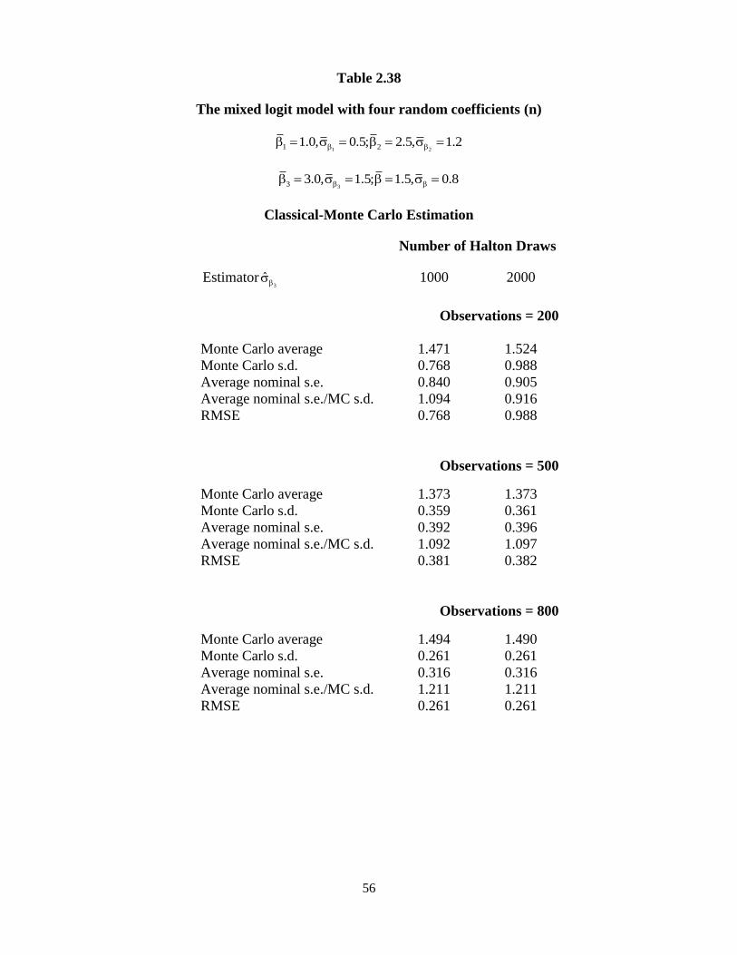
56

Table 2.38

The mixed logit model with four random coefficients (n)

1 21 21.0, 0.5; 2.5, 1.2

33 3.0, 1.5; 1.5, 0.8



Estimator3

ˆ 1000 2000

Observations = 200





RMSE 0.768 0.988

Observations = 500





RMSE 0.381 0.382

Observations = 800





RMSE 0.261 0.261

57

Table 2.39

The mixed logit model with four random coefficients (o)

1 21 21.0, 0.5; 2.5, 1.2

33 3.0, 1.5; 1.5, 0.8



Estimator 1000 2000

Observations = 200





RMSE 0.742 1.070

Observations = 500





RMSE 0.252 0.253

Observations = 800





RMSE 0.200 0.200

58

Table 2.40

The mixed logit model with four random coefficients (p)

1 21 21.0, 0.5; 2.5, 1.2

33 3.0, 1.5; 1.5, 0.8




Observations = 200





RMSE 0.705 0.952

Observations = 500





RMSE 0.396 0.418

Observations = 800





RMSE 0.337 0.355

59

CHAPTER 3 PRETEST ESTIMATION IN THE RANDOM PARAMETERS

LOGIT MODEL

3.1 Introduction

In this chapter, we use quasi-Monte Carlo sampling experiments to examine the

properties of pretest estimators in the random parameters logit (RPL) model. The pretests are for

the presence of random parameters. We study the Lagrange multiplier (LM), likelihood ratio

(LR) and Wald tests, using conditional logit as the restricted model. If the model coefficients are

not random, then the mixed logit model reduces to the simpler conditional logit model. The most

commonly used test procedures for this purpose are the Wald (or t-) test and the likelihood ratio

test for the significance of the random components of the coefficients. The problem is that in

order to implement these tests the mixed logit model must be estimated. It would be much faster

to implement a Lagrange multiplier test, as the restricted estimates come from the conditional

logit model, which is easily estimated.

We use quasi-Monte Carlo experiments in the context of one and two parameter choice

models with four alternatives to examine the risk properties of pretest estimator based on LM,

LR and Wald tests. We explore the power of the three tests for the random parameters by

calculating the empirical 90th and 95th percentile values of the three test statistic distributions

and examine rejection rates of the three tests by using the empirical 90th and 95th percentile

values as the critical values for 10% and 5% significance level. We find the pretest estimators

based on the LR and Wald statistics have RMSE that is less than that of the random parameters

logit model when the parameter variance is small, but that RMSE of the pretest estimators is

worse than that of the random parameters logit model over the remaining parameter space. The

LR and Wald tests exhibit properties of consistent tests, with the power approaching one as the

specification error increases. The power of LR and Wald tests decreases with increases in the

60

mean of the coefficient distribution reflecting an increase in model signal-to-noise ratio. The

ratios of LM-based pretest estimator RMSE to that RMSE of the random parameters logit model

rise and become further away from one with increases in the standard deviation of the parameter

distribution as a result of the general failure of the LM test in this application.

The plan of the chapter is as follows. In Section 3.2, we show and summarize the mean

squared error properties of the pretest estimator based on LM, LR and Wald tests, and the size

corrected rejection rates of these three tests. Some conclusions and recommendations are given

in Section 3.3.

3.2 Pretest Estimators

Even though the mixed logit model is highly flexible, it requires the use of time-

consuming simulation to obtain empirical estimates. It is desirable to have a specification test to

determine whether the mixed logit is needed or not. The likelihood ratio (LR) and Wald tests are

the most popular test procedures used for testing the significance of coefficient estimates. The

problem is that in order to implement these tests the mixed logit model must be estimated. It is

much faster to implement a Lagrange Multiplier (LM) test. It is interesting and important to

examine the power of these three tests for the presence of the random coefficients in the mixed

logit model. We use quasi-Monte Carlo experiments in the context of one and two parameters

choice model with four alternatives to examine the properties of pretest estimators in the random

parameters logit model with LR, LM and Wald tests.

3.2.1 One Parameter Model Results

In the one random parameter model, we set four different values for the parameter mean,

{0.5, 1.5, 2.5, 3.0}. Corresponding to each value of the mean , we set six different values

for the standard deviation of the parameter distribution, {0, 0.15, 0.3, 0.8, 1.2, 1.8}. We

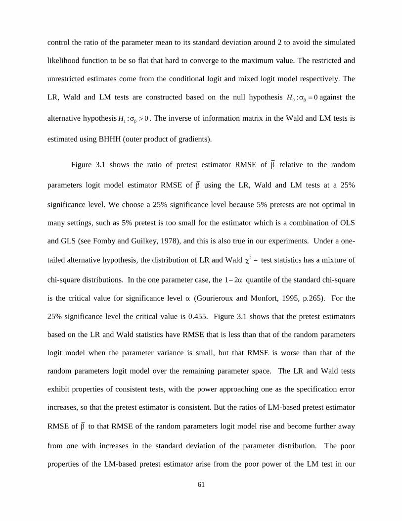
61

control the ratio of the parameter mean to its standard deviation around 2 to avoid the simulated

likelihood function to be so flat that hard to converge to the maximum value. The restricted and

unrestricted estimates come from the conditional logit and mixed logit model respectively. The

LR, Wald and LM tests are constructed based on the null hypothesis 0 : 0H against the

alternative hypothesis 1 : 0H . The inverse of information matrix in the Wald and LM tests is

estimated using BHHH (outer product of gradients).

Figure 3.1 shows the ratio of pretest estimator RMSE of relative to the random

parameters logit model estimator RMSE of using the LR, Wald and LM tests at a 25%

significance level. We choose a 25% significance level because 5% pretests are not optimal in

many settings, such as 5% pretest is too small for the estimator which is a combination of OLS

and GLS (see Fomby and Guilkey, 1978), and this is also true in our experiments. Under a one-

tailed alternative hypothesis, the distribution of LR and Wald 2 test statistics has a mixture of

chi-square distributions. In the one parameter case, the 1 2 quantile of the standard chi-square

is the critical value for significance level (Gourieroux and Monfort, 1995, p.265). For the

25% significance level the critical value is 0.455. Figure 3.1 shows that the pretest estimators

based on the LR and Wald statistics have RMSE that is less than that of the random parameters

logit model when the parameter variance is small, but that RMSE is worse than that of the

random parameters logit model over the remaining parameter space. The LR and Wald tests

exhibit properties of consistent tests, with the power approaching one as the specification error

increases, so that the pretest estimator is consistent. But the ratios of LM-based pretest estimator

RMSE of to that RMSE of the random parameters logit model rise and become further away

from one with increases in the standard deviation of the parameter distribution. The poor

properties of the LM-based pretest estimator arise from the poor power of the LM test in our

62

experiments. It is interesting that even though the pretest estimator based on the LR and Wald

statistics are consistent, the maximum risk ratio based on the LR and Wald tests increases in the

parameter mean . The range over which the risk ratio is less than one also increases in the

mean of the parameter distribution . It implies that the power of LR and Wald tests for testing

random coefficients are sensitive to the parameter mean and standard deviation in the context of

the RPL model and leads us to explore the power of these three tests for presence of random

coefficients in the RPL model.

Figure 3.1: Pretest Estimator RMSE Mixed Logit Estimator RMSE :

One Random Parameter Model

63

To explore the power of these three tests for the presence of the random coefficient in the

mixed logit model further, we calculate the empirical 90th and 95th percentile value of the LR,

Wald and LM statistic distributions given the different combinations of means and standard

deviations of the parameter distribution in the one random parameter model. The results in Table

3.1 show that the Monte Carlo 90th

and 95th

percentile values of the three test statistic

distributions change with the changes in the mean and standard deviation of parameter

distribution. In general, the Monte Carlo critical values with different parameter means are

neither close to 1.64 and 2.71 (the 1 2 quantile of standard chi-square statistics for 10% and

5% significance level respectively) nor to the usual critical values 2.71 and 3.84. When 0.5

and 0 , the 90th

and 95th

empirical percentiles of LR, Wald and LM in our experiments both

are greater than the asymptotic critical values 1.64 and 2.71. With increases in the true standard

deviation of the coefficient distribution, the 90th

and 95th

empirical percentiles increase for the

LR and Wald statistics, indicating that these tests will have some power in choosing the correct

model with random coefficients. The corresponding percentile values based on the LM statistics

decline, meaning that the LM test has declining power. An interesting feature of Table 3.1 is that

most empirical percentile values based on the LR and Wald statistic distributions decrease in the

parameter mean . Since the parameter mean should not influence the power of LR and Wald

tests, it implies that the power of tests may be affected by the ratio of parameter mean to

parameter standard deviation, which is also called the signal-to-noise ratio.

The results based on the empirical percentiles of the LR, Wald and LM statistic

distributions imply the rejection rates of the three tests will vary depending on the mean and

standard deviation of the parameter distribution. To get the rejection rate for the three tests, we

choose the “correct” chi-square critical values 1.64 and 2.71 for 10% and 5% significance levels

with one degree of freedom. Table 3.2 provides the percentage of rejecting the null hypothesis

64

0 , using critical value 1.64 and 2.71. When the null hypothesis is true, most empirical

percentage rates of LR test rejecting the true null hypothesis are less than the nominal rejection

rates 10% and 5%, and become further away from the nominal rejection rates with increases in

the parameter mean . All empirical rejection rates of Wald and LM tests given a true null

hypothesis are greater than the related expected percentage rates. The size of the LR test is too

large, and the size of LM and Wald tests is too small.

Figure 3.2 contains graphs based on the results of Table 3.2. From Figure 3.2, we can see

the changes in the rejection rates of these three tests with increases in the mean and standard

deviation of the parameter distribution respectively. We find the rejection frequency of the LR

and Wald statistics declines in the mean of the parameter distribution.

Due to the different sizes of the three tests, power comparisons are invalid. We use the

Monte Carlo percentile values for each combination of parameter mean and standard deviation as

the critical value to correct the size of the three tests. Table 3.3 provides the size corrected

rejection rates for the three tests. The size corrected rejection rates for the LR and Wald tests

increase in the standard deviation of the coefficient distribution as expected. Based on the

results, there is not too much difference between these two size corrected tests. As expected the

power of these two tests still declines with increases in the parameter mean. In our experiments,

at the 10% and 5% significance levels, the LM test shows the weakest power for the presence of

the random coefficient among the three tests. Graphs in Figure 3.3 are based on the results of

Table 3.3. After adjusting the size of the test, the power of LR test declines slowly in the

parameter mean. The results of the power of these three tests are consistent with the results of

pretest estimators based on these three tests.

65

Table 3.1: 90th

and 95th

Empirical Percentiles of Likelihood Ratio, Wald and Lagrange Multiplier Test Statistical Distributions


LR-90th LR-95

th Wald-90

th Wald-95

th LM-90

th LM-95

th

0.5 0.00 1.927 3.267 4.006 5.917 2.628 3.576

0.5 0.15 1.749 2.755 3.850 5.425 2.749 3.862

0.5 0.30 2.239 3.420 4.722 6.210 2.594 3.544

0.5 0.80 6.044 7.779 9.605 11.014 2.155 3.043

0.5 1.20 12.940 15.684 14.472 15.574 1.712 2.344

0.5 1.80 26.703 31.347 19.225 19.950 1.494 2.041

1.5 0.00 1.518 2.668 3.671 5.672 2.762 3.972

1.5 0.15 1.541 2.414 3.661 5.443 3.020 4.158

1.5 0.30 1.837 3.364 4.361 6.578 3.048 4.308

1.5 0.80 5.753 7.451 8.603 10.424 2.496 3.489

1.5 1.20 11.604 13.953 12.930 13.974 1.825 2.376

1.5 1.80 24.684 28.374 17.680 18.455 1.346 1.947

2.5 0.00 0.980 1.727 2.581 4.017 2.978 4.147

2.5 0.15 1.020 1.858 2.598 4.256 2.976 4.317

2.5 0.30 1.217 2.235 2.751 4.616 3.035 4.429

2.5 0.80 2.766 4.667 6.387 8.407 3.119 4.315

2.5 1.20 6.321 8.643 9.700 11.598 2.714 3.832

2.5 1.80 18.018 20.828 14.895 15.822 2.189 3.275

3.0 0.00 1.042 1.720 2.691 4.264 3.455 4.594

3.0 0.15 1.040 1.941 2.548 4.878 3.285 4.441

3.0 0.30 1.260 2.114 3.068 5.124 3.164 4.324

3.0 0.80 2.356 3.167 4.915 7.106 3.073 4.198

3.0 1.20 4.610 6.570 8.086 10.296 2.917 4.224

3.0 1.80 13.261 15.622 12.960 14.052 2.579 3.478

Note: *Testing 0 : 0H ; One tail critical values are 1.64 (10%) and 2.71 (5%), compared to the usual values

2.71 and 3.84 respectively.

66

Table 3.2: Rejection Rate of Likelihood Ratio, Wald and Lagrange Multiplier Test Statistic Distributions


ˆ *ˆ( )se *ˆ( )se LR-10%** LR-5%** Wald-10%** Wald-5%** LM-10%** LM-5%**

0.5 0.00 0.123 0.454 0.122 0.065 0.219 0.155 0.204 0.095

0.5 0.15 0.125 0.461 0.113 0.051 0.233 0.164 0.200 0.101

0.5 0.30 0.125 0.460 0.143 0.072 0.281 0.214 0.184 0.093

0.5 0.80 0.135 0.416 0.472 0.348 0.665 0.587 0.161 0.061

0.5 1.20 0.153 0.391 0.816 0.722 0.916 0.882 0.109 0.036

0.5 1.80 0.195 0.438 0.996 0.989 1.000 0.999 0.084 0.021

1.5 0.00 0.242 0.593 0.092 0.048 0.199 0.139 0.215 0.102

1.5 0.15 0.243 0.586 0.090 0.042 0.215 0.148 0.225 0.116

1.5 0.30 0.243 0.567 0.115 0.068 0.236 0.160 0.233 0.119

1.5 0.80 0.247 0.439 0.390 0.264 0.582 0.461 0.184 0.083

1.5 1.20 0.261 0.391 0.777 0.659 0.897 0.816 0.116 0.037

1.5 1.80 0.291 0.443 0.995 0.990 0.999 0.996 0.075 0.016

2.5 0.00 0.416 0.910 0.058 0.022 0.143 0.090 0.216 0.111

2.5 0.15 0.416 0.889 0.064 0.023 0.146 0.095 0.221 0.122

2.5 0.30 0.410 0.853 0.070 0.031 0.159 0.101 0.221 0.119

2.5 0.80 0.392 0.714 0.176 0.106 0.335 0.235 0.229 0.121

2.5 1.20 0.392 0.537 0.471 0.342 0.641 0.539 0.221 0.100

2.5 1.80 0.412 0.453 0.949 0.898 0.985 0.959 0.166 0.068

3.0 0.00 0.519 1.131 0.052 0.028 0.139 0.099 0.229 0.140

3.0 0.15 0.508 1.062 0.060 0.026 0.140 0.096 0.248 0.128

3.0 0.30 0.514 0.975 0.076 0.030 0.162 0.113 0.237 0.130

3.0 0.80 0.489 0.910 0.135 0.074 0.256 0.190 0.226 0.117

3.0 1.20 0.478 0.701 0.304 0.199 0.465 0.389 0.221 0.114

3.0 1.80 0.479 0.505 0.808 0.714 0.909 0.858 0.217 0.095

*The average nominal standard errors of estimated parameter mean and standard deviation

**Testing 0 : 0H ; One-tail critical values are 1.64 (10%) and 2.71 (5%)

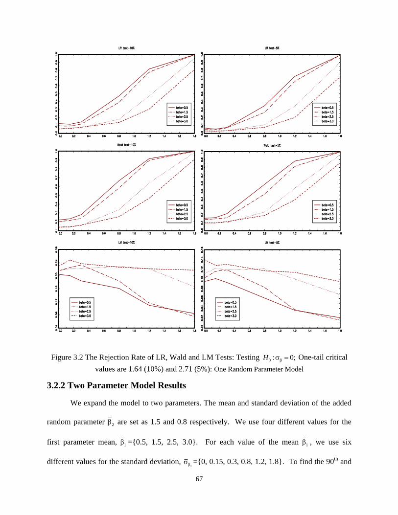
67

Figure 3.2 The Rejection Rate of LR, Wald and LM Tests: Testing 0 : 0;H One-tail critical

values are 1.64 (10%) and 2.71 (5%): One Random Parameter Model

3.2.2 Two Parameter Model Results

We expand the model to two parameters. The mean and standard deviation of the added

random parameter 2 are set as 1.5 and 0.8 respectively. We use four different values for the

first parameter mean, 1 ={0.5, 1.5, 2.5, 3.0}. For each value of the mean 1 , we use six

different values for the standard deviation, 1

={0, 0.15, 0.3, 0.8, 1.2, 1.8}. To find the 90th

and

68

95th

empirical percentiles of LR, Wald and LM test statistic distributions, we set 1 2

0

first. In the two parameters model, the LR, Wald and LM tests are constructed based on the joint

null hypothesis 10 : 0H and

20 against the alternative hypothesis

11 : 0H or 2

0 or

10 and

20 . Figure 3.4 shows the ratios of the pretest estimator RMSE of 1 and 2 to

the random parameters logit model estimator RMSE of 1 and 2 based on the joint LR, Wald

and LM tests at a 25% significance level. Here we use 2 2

1 1

1 1(1) (2)

2 2 , the weighted chi-

square statistics, as the critical value for 25%, significance level, 2.048 (Gourieroux and

Monfort, 1995, p.261). The joint LR and Wald tests show properties of consistent tests. The

maximum risk ratio based on the joint LR and Wald tests still increases in the parameter mean.

In the two parameter model, the pretest estimators based on the joint LR and Wald statistics have

larger RMSE than that of the random parameters logit model. The properties of the joint LM-

based pretest estimator are also poor in two parameter model. Table 3.4 reports the 90th

and 95th

empirical percentiles of the joint LR, Wald and LM test statistic distributions. They are different

with different combinations of parameters mean and standard deviations. When the parameters

standard deviations are zero, 1 2

0 , the empirical 90th

and 95th

percentile value of the joint

LR test statistic distribution are all less than the according weighted chi-square statistic critical

values 3.655 and 4.916. However, the empirical 90th

and 95th

percentile value of the joint Wald

test statistic distribution are all greater than the according weighted chi-square statistic critical

values. Both of them increase with increases in the parameters standard deviations as expected.

The Monte Carlo empirical percentiles of the joint LM test statistic distributions are also greater

than the weighted chi-square statistics and are not sensitive to parameters standard deviations.

Then we use the weighted chi-square statistic critical values 3.655 and 4.916 to find the rejection

rate of these three tests.

69

Table 3.3: Size Corrected Rejection rates of LR, Wald and LM Test Statistic Distributions:


LR -10% LR -5% Wald -10% Wald -5% LM -10% LM -5%

0.5 0.00 0.100 0.050 0.100 0.050 0.100 0.050

0.5 0.15 0.094 0.035 0.093 0.036 0.108 0.060

0.5 0.30 0.121 0.055 0.123 0.056 0.099 0.049

0.5 0.80 0.431 0.287 0.498 0.336 0.066 0.028

0.5 1.20 0.792 0.676 0.834 0.746 0.040 0.016

0.5 1.80 0.995 0.980 0.999 0.991 0.022 0.005

1.5 0.00 0.100 0.050 0.100 0.050 0.100 0.050

1.5 0.15 0.100 0.043 0.098 0.047 0.112 0.056

1.5 0.30 0.124 0.068 0.124 0.067 0.115 0.058

1.5 0.80 0.407 0.269 0.383 0.240 0.078 0.031

1.5 1.20 0.788 0.663 0.758 0.616 0.035 0.014

1.5 1.80 0.995 0.990 0.995 0.988 0.011 0.005

2.5 0.00 0.100 0.050 0.100 0.050 0.100 0.050

2.5 0.15 0.101 0.060 0.100 0.056 0.099 0.052

2.5 0.30 0.119 0.069 0.110 0.065 0.103 0.057

2.5 0.80 0.256 0.166 0.242 0.173 0.104 0.051

2.5 1.20 0.565 0.460 0.544 0.444 0.082 0.037

2.5 1.80 0.971 0.942 0.961 0.931 0.062 0.022

3.0 0.00 0.100 0.050 0.100 0.050 0.100 0.050

3.0 0.15 0.099 0.058 0.096 0.059 0.089 0.046

3.0 0.30 0.120 0.071 0.114 0.080 0.083 0.042

3.0 0.80 0.197 0.133 0.192 0.121 0.079 0.042

3.0 1.20 0.403 0.294 0.392 0.282 0.072 0.041

3.0 1.80 0.873 0.803 0.859 0.764 0.051 0.031

Testing 0 : 0H ; using Monte Carlo percentile values as the critical values to adjust the size the LR, Wald and LM tests

70

Figure 3.3 The Size Corrected Rejection Rates: One Random Parameter Model

71

Figure 3.4 Pretest Estimation RMSE Mixed Logit Estimation RMSE :

Two Random Parameter Model, RMSE of 2 2

1 2 2 21 1

ˆ ˆ ˆ( ) ( ) /NSAM NSAM

n n

NSAM

72

Table 3.4: 90th

and 95th

Empirical Percentiles of Likelihood Ratio, Wald and Lagrange Multiplier Test Statistical Distributions

Two Random Parameter Model

1 1

2 2

LR-90th LR-95

th Wald-90

th Wald-95

th LM-90

th LM-95

th

0.5 0.00 1.5 0.0 2.771 4.157 5.054 6.923 4.725 6.345

0.5 0.15 1.5 0.8 13.583 17.001 13.148 14.118 4.164 5.242

0.5 0.30 1.5 0.8 13.504 16.043 13.060 14.156 4.208 5.420

0.5 0.80 1.5 0.8 14.961 17.867 12.496 13.157 4.052 5.062

0.5 1.20 1.5 0.8 19.940 23.966 13.536 14.305 4.168 5.215

0.5 1.80 1.5 0.8 29.429 32.083 15.208 16.081 3.989 5.218

1.5 0.00 1.5 0.0 2.515 3.467 4.681 5.749 5.057 6.610

1.5 0.15 1.5 0.8 12.645 15.466 11.961 13.448 5.991 7.689

1.5 0.30 1.5 0.8 11.955 14.415 11.498 12.641 5.881 7.444

1.5 0.80 1.5 0.8 12.341 14.569 11.022 12.017 4.480 5.601

1.5 1.20 1.5 0.8 15.529 17.472 11.760 12.860 4.478 5.699

1.5 1.80 1.5 0.8 22.300 25.700 13.321 14.155 4.682 5.639

2.5 0.00 1.5 0.0 2.682 3.699 4.268 5.739 5.254 6.415

2.5 0.15 1.5 0.8 10.449 13.120 9.820 11.137 4.920 6.368

2.5 0.30 1.5 0.8 9.998 12.437 9.707 10.986 5.051 6.230

2.5 0.80 1.5 0.8 10.388 12.690 9.554 10.657 4.714 6.092

2.5 1.20 1.5 0.8 14.168 17.001 10.527 11.433 4.552 5.829

2.5 1.80 1.5 0.8 21.625 24.694 12.815 13.704 4.994 6.248

3.0 0.00 1.5 0.0 2.979 4.553 4.199 5.907 5.334 6.995

3.0 0.15 1.5 0.8 9.185 11.450 8.493 10.215 4.434 5.923

3.0 0.30 1.5 0.8 8.384 10.388 8.262 9.7540 4.245 5.418

3.0 0.80 1.5 0.8 8.219 10.083 8.499 10.010 4.486 5.716

3.0 1.20 1.5 0.8 13.704 15.917 10.058 10.967 4.972 6.353

3.0 1.80 1.5 0.8 20.939 23.476 12.454 13.282 5.273 6.544

73

Table 3.5 shows the rejection rates of the three joint tests based on the weighted chi-square

statistic critical values for 10% and 5% significance level. The results are consistent with the

Table 3.4. When the null hypothesis is true, the joint LR test reject the true null hypothesis less

frequently than the nominal rejection rates 10% and 5%. And the Monte Carlo rejection rates of

the joint Wald test are greater than the nominal rejection rates 10% and 5%. They become closer

to the nominal rejection rates with increases in the parameter mean 1 . Figure 3.5 shows the

graphs based on the results of Table 3.5. They almost have the same trends as the one parameter

case. The rejection frequency of the joint LR and Wald statistics decreases in the mean of the

parameter distribution 1 .

To compare the power of these three joint tests in the two parameters case, we also

correct the size of the three joint tests using the Monte Carlo empirical critical values for 10%

and 5% significance level. Table 3.6 provides the size corrected rejection rates for the three joint

tests. Figure 3.6 presents the graphs based on the Table 3.6. As in the one parameter case, the

joint LM test shows the weakest power for the presence of the random coefficient. The power of

the joint LR and Wald tests decreases in the mean of the parameter distribution 1.

3.3 Conclusions and Discussion

. There are two major findings regarding testing for the presence of random parameters

from our Monte Carlo experiments, neither of which we anticipated. First, the LM test should not

be used in the random parameters logit model to test the null hypothesis that the parameters are

randomly distributed across the population, rather than being fixed population parameters. In the

one parameter model Monte Carlo experiment, the size of the LM test is approximately double

the nominal level of Type I error.

74

Table 3.5: Rejection Rate of Likelihood Ratio, Wald and Lagrange Multiplier Test Statistic Distributions


1 1

2 2

LR-10% LR-5% Wald-10% Wald-5% LM-10% LM-5%

0.5 0.00 1.5 0.0 0.064 0.032 0.169 0.105 0.164 0.088

0.5 0.15 1.5 0.8 0.761 0.658 0.923 0.867 0.140 0.063

0.5 0.30 1.5 0.8 0.750 0.636 0.923 0.850 0.141 0.076

0.5 0.80 1.5 0.8 0.825 0.721 0.953 0.908 0.132 0.054

0.5 1.20 1.5 0.8 0.967 0.942 0.990 0.982 0.136 0.057

0.5 1.80 1.5 0.8 1.000 0.998 1.000 1.000 0.120 0.060

1.5 0.00 1.5 0.0 0.045 0.026 0.147 0.087 0.191 0.105

1.5 0.15 1.5 0.8 0.652 0.532 0.806 0.707 0.296 0.167

1.5 0.30 1.5 0.8 0.618 0.489 0.785 0.673 0.260 0.153

1.5 0.80 1.5 0.8 0.708 0.594 0.871 0.756 0.168 0.070

1.5 1.20 1.5 0.8 0.862 0.768 0.954 0.898 0.161 0.080

1.5 1.80 1.5 0.8 0.986 0.964 0.997 0.993 0.189 0.080

2.5 0.00 1.5 0.0 0.051 0.014 0.129 0.068 0.206 0.118

2.5 0.15 1.5 0.8 0.543 0.416 0.704 0.552 0.193 0.100

2.5 0.30 1.5 0.8 0.503 0.356 0.660 0.505 0.215 0.114

2.5 0.80 1.5 0.8 0.530 0.394 0.679 0.529 0.172 0.087

1.5 1.20 1.5 0.8 0.827 0.728 0.898 0.813 0.185 0.085

2.5 1.80 1.5 0.8 0.974 0.956 0.992 0.977 0.231 0.109

3.0 0.00 1.5 0.0 0.074 0.040 0.137 0.071 0.190 0.120

3.0 0.15 1.5 0.8 0.466 0.346 0.604 0.435 0.143 0.083

3.0 0.30 1.5 0.8 0.427 0.304 0.575 0.391 0.146 0.068

3.0 0.80 1.5 0.8 0.372 0.252 0.514 0.362 0.182 0.077

3.0 1.20 1.5 0.8 0.716 0.596 0.847 0.722 0.206 0.104

3.0 1.80 1.5 0.8 0.985 0.955 0.990 0.972 0.215 0.118

75

Figure 3.5: The Rejection Rate of LR, Wald and LM Tests: Two Random Parameter Model

76

Table 3.6: Size Corrected Rejection Rates of LR, Wald and LM Test Statistic Distributions


1 1

2 2

LR-10% LR-5% Wald-10% Wald-5% LM-10% LM-5%

0.5 0.00 1.5 0.0 0.100 0.050 0.100 0.050 0.100 0.050

0.5 0.15 1.5 0.8 0.846 0.718 0.857 0.714 0.074 0.025

0.5 0.30 1.5 0.8 0.833 0.707 0.843 0.695 0.079 0.024

0.5 0.80 1.5 0.8 0.887 0.792 0.907 0.740 0.065 0.028

0.5 1.20 1.5 0.8 0.983 0.959 0.979 0.928 0.068 0.023

0.5 1.80 1.5 0.8 1.000 1.000 1.000 0.994 0.068 0.027

1.5 0.00 1.5 0.0 0.100 0.050 0.100 0.050 0.100 0.050

1.5 0.15 1.5 0.8 0.752 0.672 0.722 0.625 0.157 0.084

1.5 0.30 1.5 0.8 0.734 0.638 0.697 0.585 0.146 0.074

1.5 0.80 1.5 0.8 0.831 0.727 0.781 0.661 0.064 0.027

1.5 1.20 1.5 0.8 0.932 0.876 0.912 0.840 0.071 0.025

1.5 1.80 1.5 0.8 0.996 0.990 0.994 0.985 0.076 0.021

2.5 0.00 1.5 0.0 0.100 0.050 0.100 0.050 0.100 0.050

2.5 0.15 1.5 0.8 0.668 0.542 0.623 0.450 0.084 0.047

2.5 0.30 1.5 0.8 0.625 0.499 0.573 0.379 0.094 0.043

2.5 0.80 1.5 0.8 0.634 0.526 0.612 0.443 0.069 0.034

2.5 1.20 1.5 0.8 0.894 0.821 0.861 0.742 0.071 0.036

2.5 1.80 1.5 0.8 0.988 0.974 0.984 0.962 0.085 0.042

3.0 0.00 1.5 0.0 0.100 0.050 0.100 0.050 0.100 0.050

3.0 0.15 1.5 0.8 0.562 0.380 0.532 0.298 0.072 0.024

3.0 0.30 1.5 0.8 0.517 0.335 0.495 0.279 0.055 0.020

3.0 0.80 1.5 0.8 0.448 0.286 0.450 0.251 0.059 0.027

3.0 1.20 1.5 0.8 0.777 0.626 0.784 0.620 0.080 0.034

3.0 1.80 1.5 0.8 0.992 0.966 0.985 0.940 0.096 0.036

77

Figure 3.6: The Size Corrected Rejection Rates: Two Random Parameter Model

78

Then, the rejection rate decreases as the degree of the specification error rises, which is in direct

contrast to the properties a consistent test. This is the most troubling and disappointing finding, as

the LM test is completed in a fraction of a second, while LR and Wald tests requiring estimation of

the mixed logit model are time consuming to estimate even with a limited number of Halton draws.

This outcome resulted despite our use of the now well established adjusted chi-square critical value

for one-tail tests on the boundary of a parameter space. This outcome is also not due to

programming errors on our part, as our Gauss code produces estimates and LM test statistic values

that are the same, allowing for convergence criteria differences, as those produced by NLOGIT 4.0.

In the one parameter problem the likelihood ratio test had size close to the nominal level, while the

Wald test rejected the true null hypothesis at about twice the nominal level.

Our second finding is that LR and Wald test performance depends on the “signal-to-noise”

ratio, that is, the ratio of the mean of the random parameter distribution relative to its standard

deviation. When this ratio is larger the LR and Wald tests reject less frequently the null hypothesis

that the parameter is fixed rather than random. Upon reflection, this makes perfect sense. When the

parameter mean is large relative to its standard deviation then the test will have less ability to

distinguish between random and fixed parameters. The “skinny” density function of the population

parameter looks like a “spike” to the data. When the ratio of the mean of the random parameter

distribution relative to its standard deviation is large it matters less whether one chooses conditional

logit or mixed logit, from the point of view of estimating the population mean parameter. This

shows up in lower size-corrected power for the LR and Wald tests when signal is large relative to

noise. It also shows up in the risk of the pretest estimator relative to that of the mixed logit

estimator. For the portion of the parameter space where the relative risk is greater than one, as the

79

signal increases relative to noise the relative risk function increases, indicating that pretesting is a

less preferred strategy.

In the one parameter case the LR test is preferred overall. For the case when the signal-to-

noise ratio is not large the empirical critical values, under the null, are at least somewhat close to the

one-tail critical values 1.64 (10%) and 2.71 (5%) from the mixture of chi-square distributions.

When the signal-to-noise ratio increases the similarity between the theoretically justified critical

values and the test statistic percentiles becomes less clear. The Wald test statistic percentiles are not

as close to the theoretically true values as for the LR test statistic. The LM test statistic percentiles

under the null are between those of the LR and Wald test statistic distribution, but not

encouragingly close to the theoretically true values.

In the two random parameters case, we vary the value of one standard deviation parameter,

staring from 0, while keeping the other standard deviation parameter fixed at a nonzero parameter.

We observe however, that the empirical percentiles of the joint LR test statistics are less than the

weighted chi-square percentile values 3.655 (10%) and 4.916 (5%). Once again the rejection rate

profile of the LM test is flat, indicating that it is not more likely to reject the null hypothesis at

larger parameter standard deviation values. The “size corrected” rejection rates are not strictly

correct. In them we observe that the LR and Wald tests reject at a higher rate at higher signal-to-

noise ratios. Further, in the two parameters case the relative risk of the pretest estimator based on

the LR and Wald test statistics are always greater than one. The pretesting strategy is not to be

recommended under our Monte Carlo design.

Interesting questions arising from the Monte Carlo experiment results are: (1) Why does the

power of LR and Wald tests for the presence of the random coefficient declines in the parameter

80

mean and (2) How can we refine the LM test in the setting of the random parameters logit model.

The Lagrange Multiplier test is developed by Aitchison and Silvey (1958) and Silvey (1959) in

association with the constrained optimization problem. In our setting, the Lagrangian function is:

ln ( ) ( ( ) )L c q

where ln ( )L is the log-likelihood function, which subject to the constraints ( ( ) ) 0c q . The

related first-order conditions are:

ln ( ) ( )0

( ) 0

L c

c q

Under the standard assumptions of the LM test, we know

1ˆ( ) ~ (0, ( ) )n N I

and

1/2 1( ) ( )ˆ ~ 0, ( )'

c cn N I

Based on the first-order conditions of the Lagrangian function, we have

1 1ˆ ˆ ˆ ˆ( ) ( ) ln ( ) ln ( )ˆ ˆ ˆ ˆ( ) ( )

ˆ ˆ ˆ

c c L LI I

From the above results, the LM statistic has the asymptotic 2 distribution. The asymptotic

distribution of the LM statistic is derived from the distribution of Lagrange multiplier, which

essentially based on the asymptotic normality of the score vector. In the Lagrangian function, the

log-likelihood function is subject to the equality constraints. The weak power of the LM test for the

presence of the random coefficient is caused by the failure of taking into account the properties of

the one-tail alternative hypothesis. Gourieroux, Holly and Monfort (1982) and Gourieroux and

Monfort (1995) extended the LM test to the Kuhn-Tucker multiplier test and showed that it is

81

asymptotically equivalent to the LR and Wald tests. However, computing the Kuhn-Tucker

multiplier test is complicated. In the Kuhn-Tucker multiplier test, the duality problem replaces the

two optimization problems with inequality and equality constraints, which is shown as follows:

0 00 0 1 0

ˆ ˆ( ) ( )1 ˆ ˆ ˆmin ( ) ( ) ( )g g

In

Subject to 0 where 0 and 0 are the equality constrained estimators. Compared to the

standard LM test, the Kuhn-Tucker multiplier test uses 0ˆ( ) to adjust the estimated Lagrange

Multiplier 0 . How to refine the LM test in the random parameters logit model is our future

research.

82

CHAPTER 4 SHRINKAGE ESTIMATION IN THE RANDOM

PARAMETERS LOGIT MODEL

4.1 Introduction

In this chapter we explore a problem that may exist in any correlated random parameters model.

When the random coefficients are correlated, the parameters we estimate in the random parameters

logit model are the mean and covariance matrix of random coefficients’ distributions. In the

covariance matrix , there are K variances and ( 1) / 2K K covariance terms that need to be

estimated, when the number of correlated random coefficients is K . Allowing the random

parameters to be correlated introduces potentially many new parameters which may be difficult to

estimate. For the purpose of estimating marginal effects of changes in an explanatory variable, or

for prediction, is the estimation of the more general model advantageous? Many applied workers

will test the significance of the covariance parameters before deciding to rely on the fully correlated

random parameter model instead the model in which the parameters are random but uncorrelated,

which introduces only K additional parameters to estimate. Does using a pretesting strategy

improve postestimation inferences? Judge and Bock (1978) investigate in depth this question for the

linear model and conclude that over much of the parameter space the estimation mean-squared error

is worse for the pre-test estimator than the unconstrained model. This same phenomenon appears in

nonlinear models, as demonstrated by Kim and Hill (1995).

An alternative to choosing between an unrestricted model and a restricted one on the basis of

a pretest is shrinkage estimation. A shrinkage estimator is a stochastically weighted combination of

an estimator of a fully unrestricted model and a model upon which a set of constraints is imposed.

The stochastic weighting factor is a function of a test statistic for the validity of the imposed

constraints. When the test statistic is small, indicating that the constraints are compatible with the

83

data, the unrestricted estimator is “shrunk” towards the restricted estimator. When the test statistic is

large, suggesting that the constraints are not valid, the unrestricted estimator is “shrunk” less

towards the restricted estimator. In the linear model Judge and Bock (1978) show that a positive

part Stein-like estimator has lower risk than the unrestricted least squares estimator over the entire

parameter space under certain design related conditions, making the unrestricted least squares

estimator inadmissible. Furthermore, the shrinkage estimator has lower mean-squared error than the

pretest estimator over much, but not all of the parameter space. This idea has been applied with

success in nonlinear models: Adkins and Hill (1989) examine shrinkage estimators in the probit

model; Kim and Hill (1995) provide results for the nonlinear regression model with a particular

application to the Box-Cox regression model; Sapra (1993) examines the Poisson regression model;

and Ahmed and Nicol (2010) examine the nonlinear regression model.

We apply these ideas to correlated random parameters models. A positive part Stein-like

estimation rule will be applied to shrink the estimators from a fully correlated random parameters

model towards the estimator from a restricted random parameters model that constrains the

correlations among parameters to be zero. In particular we examine the behavior of pretest and

shrinkage estimators in the context of the random parameters logit model. In this model estimation

of the covariance parameters is especially difficult. (Ruud, 1996, p. 7) concludes “…that there is a

region of the parameter space of the simulated random parameters logit model where the likelihood

is quite flat with respect to all of the covariance parameters.” This feature leads to numerical

difficulties when using iterative quadratic hill climbing algorithms. Convergence to a local

maximum, much less a global maximum, of the log-likelihood function may be slow or impossible.

The numerical difficulties are manifest in even the uncorrelated random parameters logit model, as

documented recently by Chang and Lusk (2011). In addition the flatness of the log-likelihood

84

affects the precision of estimation of the maximum simulated likelihood estimator since the

asymptotic variance is the inverse of the information measure which is related to the curvature of

the log-likelihood function. Relatively flat log-likelihoods result in effects similar to collinearity in

the linear model, where estimates are imprecisely estimated and subject to large changes when the

model or data are altered.

Using extensive simulations, we find that estimating the fully correlated random parameters

model leads to generally higher mean-squared for population mean parameters, important functions

of those parameters and predictions than using Stein-like shrinkage estimator. The shrinkage

estimator also has lower mean-squared error than the pretest estimator in our experiments, which

also improves on the fully correlated random parameters model. In addition, we find that the

positive-part Stein-like estimators with more shrinkage dominate those with less. Using marketing

consumer choice data, we find the percentage of correct predicted choices is higher using the

positive-part Stein-like estimator than it using the pretest estimator.

The plan of this chapter is as follows. In the following section we present in some detail the

correlated random parameters logit model estimators. In Section 3 we describe pretest and Stein-

like estimators. This is followed by a description of our Monte Carlo simulation design and results.

The marketing consumer choice data and results are presented in Section 5, and we end with

conclusions, recommendations and extensions.

4.2 The Correlated Random Parameters Logit Model Estimation

When K random coefficients in the RPL model are correlated to each other, there are K variances

and ( 1) / 2K K covariance terms. Instead of estimating the elements of covariance matrix of

random coefficients directly, the Cholesky factors of , which defined as a lower triangular

85

matrix A such that 'AA , are estimated and the standard deviations of the random coefficient

distribution are calculated based on the estimated Cholesky elements. Taking the number of random

coefficients 4K as an example, the related coefficient covariance matrix and Cholesky factors

are:

(4.1)

211 11 21 31 411 12 13 14

221 22 22 32 4221 2 23 24

231 32 33 33 4331 32 3 34

241 42 43 44 4441 42 43 4

'

a a a a a

a a a a aAA

a a a a a

a a a a a

With the Cholesky factors A , the random coefficients n can be written as

n SNb A , where b is

the mean vector and SN are generated from independent standard normal distribution. Using one

observation as example, then the random coefficients for this individual is:

(4.2a)

,1111 1

,221 222 2

,331 32 333 3

,441 42 43 444 4

SN

SN

SN

SN

ab

a ab

a a ab

a a a ab

Therefore we can write each coefficient as

(4.2b)

1 1 11 ,1

2 2 21 ,1 22 ,2

3 3 31 ,1 32 ,2 33 ,3

4 4 41 ,1 42 ,2 43 ,3 44 ,4

SN

SN SN

SN SN SN

SN SN SN SN

b a

b a a

b a a a

b a a a a

The parameter means and each element of the Cholesky factors can be estimated by maximizing the

simulated log-likelihood function.

The estimated standard deviations of the parameter distribution based on the estimated Cholesky

factors are:

86

(4.3) 2ˆ ˆ ˆ( )i ij ijj

f a a , 1,2,3,4i j

The parameters in the fully correlated RPL model are:

(4.4) 1 11 21 , 1( , , , , , , , , )f k kk k ka a a a

When the lower triangular matrix A becomes diagonal matrix, the coefficient covariance matrix is

diagonal matrix and the fully correlated RPL model reduces to the simpler uncorrelated RPL model

and the related parameters are:

(4.5) 1 11( , , , , , )u k kka a or

11( , , , , , )kk

4.3 The Pretest and Stein-like Estimators in the Random Parameters Logit

Model

Stein-rule estimators, following the work of Stein (1956) and James and Stein (1961), and combine

sample information with non-sample information in a way that improves the precision of the

estimation process and the quality of subsequent predictions. The Stein rule estimator is a weighted

average of the restricted and unrestricted estimators, the weight being a function of the magnitude

of the test statistic used to test the restrictions. It “shrinks” the unrestricted estimator towards the

restricted estimator, and the test statistic determines the extent of shrinkage. Shrinkage estimators

are biased, but may have lower estimation or prediction mean squared error, or risk. It is well

known that the Stein-rule estimator outperforms the maximum likelihood estimator (MLE) in the

context of the normal linear regression model under certain conditions. There have been a number

of studies on Stein-like estimation in the context of nonlinear models. Adkins and Hill (1989) use

the approximate normality of MLE to construct a Stein-rule estimator for the probit model by

replacing the elements of the Stein-rule used in the classical normal linear regression model with the

87

estimates of the probit model. They find that when the sample size is small (50 observations), the

Stein-like estimator outperforms the MLE in the sense that it has smaller risk over the range of

parameters considered. For larger samples, the performance of all the estimators examined

improves. The positive-part Stein-like estimation rule is superior to MLE and other Stein-rule

alternatives for small to moderate degrees of hypothesis error. Kim and Hill (1995) propose a

positive-part Stein-like estimator for the Box-Cox model and derive the asymptotic risk functions of

the maximum likelihood estimator, the restricted maximum likelihood estimator, the pretest

estimator, and the positive-part rule under a sequence of local alternatives 0 : /H R r T ,

where is a vector of constants defining the degree of hypothesis error. They show that under

information matrix weighted quadratic loss the risk of the shrinkage estimator for any 0c is

smaller than the risk of the maximum likelihood estimator, where c is a constant controlling the

degree of shrinkage.

If we use the likelihood ratio (LR), Lagrange multiplier (LM) or Wald test to test whether

the coefficient variance-covariance matrix is a diagonal matrix or not, the pretest estimator * is:

(4.6) * u

f

u cif

u cif

where u is the LR, LM or Wald test statistic for testing the coefficient covariance matrix is diagonal

matrix or not, and c is the critical value of chi-square distribution with J degrees of freedom and

significance level .

Following Kim and Hill (1995), the shrinkage or the positive-part Stein-like estimator is

a stochastically weighted convex combination of fully correlated RPL model estimates ˆf and

correlated RPL model estimates ( ˆu ):

88

(4.7) ˆ ˆ(1 )u fc c

where ( , )1 ( )(1 / )ac I u a u and ( , ) ( )aI u is the indicator function of test statistic u . The shrinkage

constant c depends on test statistic u . The constant a , chosen by the user, controls the amount of

shrinkage towards the uncorrelated RPL model estimates. The shrinkage estimator becomes the

uncorrelated RPL model estimator u when the test statistic u is less than the value of a . The larger

the value of a , the more weight give to the uncorrelated RPL model estimates. In our experiments,

we set 2a J and 2 ( 2)a J respectively to analyze how the value of a influences the

efficiency of the shrinkage estimator.

4.4 The Monte Carlo Experiments and Results

The Monte Carlo experiments are under the context of the RPL model which has no intercept term.

To satisfy the sufficient condition for minimaxity of the Stein-rule estimator, which requires the

number of restrictions strictly greater than 2, we set four random coefficients in the RPL model. The

random coefficients can be correlated to each other. Each individual still faces four mutually

exclusive alternatives on one choice occasion. The explanatory variables for each individual and

each alternative nix are generated from independent standard normal distributions. The coefficients

for each individual n are generated from multivariate normal distribution ( , )N . The mean and

variance of random coefficients are set as 1. The covariance elements of random coefficients are set

as the same value and changed from 0 to 0.8 to study how they influence the efficiency of the RPL

model estimators.

That is, we specify:

89

(4.8)

1

1

1

1

where = 0, 0.1, 0.4, 0.6, 0.8

The correlation cov( , )

var( ) var( )

i j

i j

and cov( , )i j =0, 0.1, 0.4, 0.6, 0.8. Since the variances of the

random coefficients are all equal to one, the covariance terms of random coefficients are equal to

the correlation.

The values of nix and

n are held fixed over each experiment design. The dependent

variable values niy are determined by comparing the utility of each alternative:

(4.9) 1

0

n ni ni n nj nj

ni

x xy

Otherwise

i j

The explanatory variable 1niy if individual n chooses alternative i and is 0 otherwise. The values

of the random errors ni are generated from i.i.d. extreme value type I distribution. In the

experiments, we choose the estimation sample size 200N and generate 999 Monte Carlo samples

with specific mean and covariance matrix that we set for the four random coefficients distribution in

each experiment design. Since using much fewer quasi-random numbers generated by Halton

sequences can achieve the same or even higher estimation accuracy as using pseudo-random

numbers and can reduce the computational time greatly, the Halton draws are also used here to

simulate the choice probability of the RPL model and 100 Halton draws are assigned to each

individual in this four random parameter model.

To study how the covariance elements of the random coefficients influence the estimator

efficiency, we calculate the ratio of the mean squared error (MSE) of the uncorrelated RPL model

estimates to those of the fully correlated RPL model estimates. The mean squared error of

90

uncorrelated and fully correlated RPL model estimates with parameter mean is calculated as

follows:

(4.10) Mean Squared Error (MSE) of 4 2

1 1

ˆ ˆ /NSAM

k kn k

NSAM

The likelihood ratio (LR), Wald and Lagrange multiplier (LM) tests are used to choose

between the uncorrelated RPL model and the fully correlated RPL model by testing the null

hypothesis: 0 12 13 23 14 24 34: 0, 0, 0, 0, 0, 0H against the alternative hypothesis that at

least one of covariance elements is not zero. Since the covariance elements are calculated through

the estimated Cholesky factors shown in (4.10) instead of being estimated directly, we construct the

Wald test to test the joint null hypothesis through testing the Cholesky factors:

21 31 32 41 42 430, 0, 0, 0, 0, 0.a a a a a a

(4.11)

12 21 11

13 31 11

23 31 21 32 22

14 41 11

24 41 21 42 22

34 41 31 42 32 43 33

a a

a a

a a a a

a a

a a a a

a a a a a a

Table 4.1 provides the ratios of the MSE of uncorrelated RPL model estimates to that of

correlated RPL model estimates with the covariance elements increasing from 0 to 0.8. The results

are all less than one. The uncorrelated RPL model estimators’ risks are almost one third of those of

the correlated RPL model estimators, even though the random coefficients are correlated. The ratio

of the MSE of uncorrelated RPL model estimates to that of the fully correlated RPL model

estimates reaches to the smallest value when the random coefficients are uncorrelated. However,

when the correlation of the random coefficients increases a little bit to 0.1, the ratio reaches to the

91

highest value in our Monte Carlo experiments which is close to the ratio with highly correlated

random coefficients, =0.8. When we look at the MSE of uncorrelated and fully correlated RPL

model estimator respectively, the uncorrelated RPL model estimator has bigger MSE with =0.1

and 0.8. The MSE of fully correlated RPL model reaches the highest value when =0.1. It implies

that the uncorrelated RPL model estimator may have relative bigger risk when the random

coefficients weakly or highly correlate to each other. With the correlation of the random

coefficients increases from 0.4 to 0.8, the ratios of MSE of uncorrelated RPL model estimates to the

MSE of fully correlated RPL model estimates increase as expected. The MSE of the estimated

mean and standard deviation of the random coefficient distribution with using the correlated RPL

model is almost as twice as those using the uncorrelated RPL model when the covariance of random

coefficients is 0.8.

Table 4.1: The MSE of Uncorrelated RPL model Estimates the MSE of Correlated RPL Model Estimates

cov( , )i j MSE of ˆu MSE of ˆ

f MSE of 2ˆu

MSE of2ˆ

f

0.0 0.237 0.139

0.1 0.449 0.452

0.4 0.260 0.269

0.6 0.303 0.402

0.8 0.402 0.403

The covariance elements introduce the noise during the estimation and make the estimated mean

and standard deviation of the fully correlated RPL model coefficient distrubtions have greater risk

than those of the uncorrelated RPL model. Following Ruud’s (1996) suggestion, we included two

fixed coefficients in the fully correlated RPL model. However, adding fixed coefficients doesn’t

reduce the risk of the fully correlated RPL model estimators greatly. It leads us to try to improve

92

the efficiency of the fully correlated RPL model estimators by using the pretest and positive-part

Stein-like estimators.

To study how the pretest and positive-part Stein-like estimators reduce the risk of the fully

correlated RPL model estimators, we calculate the MSEs of the estimated parameters mean,

parameters variance, parameters covariance and all estimated parameters with the pretest, positive-

part Stein-like and fully correlated RPL model estimators respectively. With the results of MSE, we

calculate the average relative loss for parameters mean, variance, covariance and all of them based

on the pretest and positive-part Stein-like estimators.

(4.12) Average Relative Loss (ARL) of 24 4 2

1 1 1

1ˆ ˆ ˆ/NSAM

k k fk kn k k NSAM

Figure 4.1 shows results based on the estimated parameters mean. In Figure 4.1, the ratios of the

LR, LM and Wald based positive-part Stein-like, pretest estimator MSE to the fully correlated RPL

model estimator MSE are all less than one. It implies that the risks of the estimated parameters

mean based on the positive-part Stein-like and pretest estimators are all smaller than those with the

fully correlated RPL model estimators. At the same time, the estimated parameters mean of the

positive-part Stein-like estimator with the shrinkage constant 2 ( 2)a J outperforms the

estimated parameters mean of the positive-part Stein-like estimator with 2a J , where J is the

degree of freedom 6, and pretest estimator. When the correlation of random coefficients increases to

0.1, the ratio of the positive-part Stein-like estimator and pretest estimator MSE to the fully

correlated RPL model estimator MSE increases, except for the ratio of the LR based pretest

estimator. It means when the random coefficients of RPL model are weakly correlated to each other,

the average relative loss of the pretest estimator and positive-part Stein-like estimator may increase.

With the correlation of random coefficients increases further to 0.8, the average relative loss of the

93

pretest and positive-part Stein-like estimators decreases first and then increases as expected. With

increases in the correlation of the random coefficients, LR, LM and Wald tests reject the null

hypothesis more frequently. The pretest estimator chooses the fully correlated RPL model estimator

more frequently as well.

Figure 4.1: The Ratios of LR, LM and Wald based Pretest, Shrinkage Estimator MSE

to the Fully Correlated RPL Model Estimator MSE (estimated parameters mean)

94

With the given value of the shrinkage constant a , the positive-part Stein-like estimator gives more

weights of the correlated RPL model estimates when the value of test statistic u used to test the null

hypothesis increases. So the average relative loss of the pretest estimator and positive part Stein-like

estimator approaches to one with increases in the correlation of the random coefficients. Compared

to the ratios of the LR and LM based pretest and positive-part Stein-like estimators MSE to the fully

correlated RPL model estimator MSE, the ratios of the Wald-based pretest, positive-part Stein-like

estimators approach to one slowly with increases in the correlation of random coefficients. Since

the Wald test uses the unconstrained estimator and the BHHH estimator of information matrix, the

larger risk of the fully correlated RPL model estimator influences the power of the Wald test for

testing the null hypothesis. With the given shrinkage constant a , the Wald based positive-part

Stein-like estimator shrinks each correlated RPL model estimator more towards the uncorrelated

RPL estimator and lead to a smaller average relative loss compared to those of LR and LM based

positive-part Stein-like estimators.

Figure 4.2 shows the results based on the estimated parameters variance which are similar to

the results of the estimated parameters mean. For the pretest and positive-part Stein-like estimators

based on the Wald test, the ratios of the positive-part Stein-like, pretest estimator MSE to the fully

correlated RPL model estimator MSE become move further away from one when the correlation of

the random coefficients increases to 0.8. It implies that even the uncorrelated RPL model is

misspecified, the estimated parameters variance has smaller risk than that with using the fully

correlated RPL model. Figure 4.3 presents the results with estimated parameters covariance. The

differences between the ratios of the pretest and Stein-rule estimators MSE to the fully correlated

RPL model estimator MSE become larger than the previous two cases. As the same as the estimated

parameters mean and variance, the ratios of the Stein-rule estimator with 2 ( 2)a J are less than

95

those of the Stein-rule estimator with 2a J . The average relative loss of the positive-part Stein-

like estimator is less than the average relative loss of the pretest estimator. Based on the results in

Figure 4.3, it implies the risk of the estimated covariance using the correlated RPL model may even

greater than that using the uncorrelated RPL model. Figure 4.4 provides the results based on the

whole uncorrelated and fully correlated RPL model estimators, 1 11( , , , , , )u k kka a and

1 11 21 , 1( , , , , , , , , )f k kk k ka a a a .

Figure 4.2: The Ratios of LR, LM and Wald based Pretest, Shrinkage estimator MSE to the Fully

Correlated RPL Model Estimator MSE (estimated variance of the coefficient distribution)

96

Figure 4.3: The Ratios of LR, LM and Wald based Pretest, Shrinkage Estimator MSE to the Fully

Correlated RPL Model Estimator MSE (estimated parameters covariance)

97

According to all of these results, the positive-part Stein-like estimators outperform the pretest

estimators in the fully correlated RPL model and the positive-part Stein-like estimator with

greater shrinkage constant 2 ( 2)a J providing smaller risk than the positive-part Stein-like

estimator with 2a J . Both the positive-part Stein-like and pretest estimators have smaller

risk than the fully correlated RPL model estimator. The Wald based pretest and positive-part

Stein-like estimators have smaller average relative loss than those based on the LR and LM test

statistics.

According to the central limit theorem, the average relative loss of estimated RPL model

estimator is asymptotically normal distributed. We construct a t-test for the average relative loss of

the pretest and positive-part Stein-like estimators with the null hypothesis 0 : 1H ARL against

the alternative hypothesis 1 : 1H ARL to test whether the mean squared error of the pretest and

positive-part Stein-like estimators are significantly smaller than that of the fully correlated RPL

model estimator. The following shows how to construct the t-test for the average relative loss of

the pretest and positive-part Stein-like estimators:

(4.12) ( 1) / ( )t ARL se ARL

and

(4.13) ( )se ARL of 2

1

ˆ ( ) / [( 1) ]NSAM

ii

RL ARL NSAM NSAM

(4.14) RL of 4 4

2 2

1 1

ˆ ˆ ˆ( ) / ( )k k fk kk k

the ARL and the standard error of the ARL are calculated as in (4.13) and (4.14) respectively. If

1.645t , the null hypothesis is rejected at 0.05 significance level and we can claim that the risk

of the pretest and positive-part Stein-like estimators is significantly smaller than the risk of the

fully correlated RPL model estimator.

98

Figure 4.4: The Ratios of LR, LM and Wald based pretest, Shrinkage Estimator MSE to the

Fully Correlated RPL Model Estimator MSE

99

Table 4.2 shows the results of the t-test of the average relative losses of the pretest and

positive-part Stein-like estimators. From Table 4.2, we can see most of the average relative

losses of the pretest and positive-part Stein-like estimators are significantly less than one at 0.01

significance level. Since the relative losses of the pretest are little bit larger than those of two

positive-part Stein-like estimators, we also construct t-tests to test the null hypothesis

Stein pretestAPL APL against the alternative hypothesis Stein pretestAPL APL . If * 1.645t , we reject

the null hypothesis at 0.05 significance level and claim that the average relative loss of the

positive-part Stein-like estimators is significantly smaller than the average relative loss of the

pretest estimators.

(4.15) * 2 2( ) / ( ) ( )Stein pretest Stein pretestt ARL ARL se ARL se ARL

From Table 4.3, we can see most of the results are significant. When the correlation of

the random coefficients is 0.1, the average relative loss of the estimated parameters mean and

variance using the positive-part Stein-like estimator with shrinkage constant 2a J is not

significantly smaller than that using the pretest estimator. However, the average relative loss of

all the estimated parameters using the positive-part Stein-like estimator with shrinkage constant

2a J is significantly smaller than that with the pretest estimator at 0.10 significance level.

When the correlation of the random coefficients is 0.1, the average relative loss of the estimated

variance using the positive-part Stein-like estimator with shrinkage constant 2( 2)a J is also

only significantly smaller than that using the pretest estimator at 0.10 significance level. The

results imply that when the random coefficients are weakly correlated, positive-part Stein-like

estimators with bigger shrinkage constant will significantly reduce the risk compared to pretest

estimators. Based on Table 4.2 and 4.3, we conclude that positive-part Stein-like estimators can

significantly reduce the risk, using MSE as the risk function, than pretest estimators.

100

Table 4.2: The t-test of the Average Relative Loss for the Pretest and Shrinkage Estimators

ARL of ARL of 2ˆii ARL of ˆ

ij ARL of 2ˆ ˆ ˆ, ,ii ij

cov pretest shrinkage1 shrinkage2 pretest shrinkage1 shrinkage2 pretest shrinkage1 shrinkage2 pretest shrinkage1 shrinkage2

0.0 0.731*** 0.495*** 0.303*** 0.672*** 0.389*** 0.189*** 0.714*** 0.300*** 0.056*** 0.676*** 0.381*** 0.176***

(0.105) (0.097) (0.113) (0.038) (0.031) (0.042) (0.013) (0.005) (0.002) (0.022) (0.019) (0.023)

0.1 0.647*** 0.598*** 0.478*** 0.651*** 0.581*** 0.472*** 0.534*** 0.231*** 0.033*** 0.643*** 0.557*** 0.442***

(0.050) (0.036) (0.052) (0.083) (0.065) (0.086) (0.014) (0.008) (0.007) (0.053) (0.041) (0.055)

0.4 0.791** 0.557*** 0.373*** 0.687*** 0.498*** 0.345*** 0.638*** 0.331*** 0.116*** 0.683*** 0.483*** 0.324***

(0.110) (0.088) (0.151) (0.049) (0.033) (0.061) (0.020) (0.018) (0.025) (0.019) (0.016) (0.025)

0.6 0.879** 0.613*** 0.443** 0.766*** 0.592*** 0.479*** 0.479*** 0.253*** 0.111*** 0.736*** 0.556*** 0.439***

(0.120) (0.080) (0.255) (0.061) (0.031) (0.069) (0.019) (0.016) (0.024) (0.018) (0.014) (0.024)

0.8 0.905*** 0.735*** 0.583*** 0.834*** 0.670*** 0.534*** 0.760*** 0.389*** 0.165*** 0.822*** 0.624*** 0.474***

(0.002) (0.014) (0.041) (0.005) (0.008) (0.019) (0.003) (0.007) (0.016) (0.004) (0.006) (0.012)

Note: ***0.01 significance level, **0.05 significance level, * 0.10 significance level; the t-test statistic for the average relative loss of the pretest and shrinkage estimators

101

Table 4.3: The t-test for the Difference of the Average Relative Loss between the Pretest and Shrinkage Estimators

ARL of ARL of 2ˆii ARL of ˆ

ij ARL of 2ˆ ˆ ˆ, ,ii ij

cov shrinkage1 shrinkage2 shrinkage1 shrinkage2 shrinkage1 shrinkage2 shrinkage1 shrinkage2

0.0 0.495** 0.303*** 0.389*** 0.189*** 0.300*** 0.056*** 0.381*** 0.176***

(0.097) (0.113) (0.031) (0.042) (0.005) (0.002) (0.019) (0.023)

0.1 0.598 0.478*** 0.581 0.472* 0.231*** 0.033*** 0.557* 0.442***

(0.036) (0.052) (0.065) (0.086) (0.008) (0.007) (0.041) (0.055)

0.4 0.557** 0.373** 0.498*** 0.345*** 0.331*** 0.116*** 0.483*** 0.324***

(0.088) (0.151) (0.033) (0.061) (0.018) (0.025) (0.016) (0.025)

0.6 0.613** 0.443* 0.592* 0.479*** 0.253*** 0.111*** 0.556*** 0.439***

(0.080) (0.255) (0.031) (0.069) (0.016) (0.024) (0.014) (0.024)

0.8 0.735*** 0.583*** 0.670*** 0.534*** 0.389*** 0.165*** 0.624*** 0.474***

(0.014) (0.041) (0.008) (0.019) (0.007) (0.016) (0.006) (0.012)

Note: ***0.01 significance level, **0.05 significance level, * 0.10 significance level; the t-test statistic for difference

between the average relative loss of the shrinkage and pretest estimators

102

Both of them significantly reduce the risk than the fully correlated RPL model estimator. In the

next section, we compare the accuracy of the predicted choice with the pretest and positive-part

Stein-like estimator using marketing consumer choice data.

4.5 The Pretest and Stein-like Estimators with Marketing Consumer Choice

Data

4.5.1 Consumer Choice Data

In this section we use marketing consumer choice data, which is a scanner panel data, to obtain

the pretest, positive-part Stein-like, uncorrelated and fully correlated RPL model estimates and

calculate the predicted choices with these four types of estimates. The original data are available

from the University of Chicago’s Kilts Center. It was collected from nine stores across two

markets over a 123-week period. The sorted data is kindly provided by Professor Danny

Weathers, Marketing Department of Louisiana State University. Each household has a choice of

four brands of 6.5-ounce cans of light tuna: StarKist-water, StarKist-oil, Chicken of the Sea-

water and Chicken of the Sea-oil. The explanatory variables are: choice-specific constants, BR1,

BR2 and BR3 for the first three brands; NETPRICE, the actual price paid by households, which

is the price of the canned tuna minus the coupon value, two dummy variables indicating whether

the brand was on featured in sales papers or displayed in stores at the time of purchase;

LOYALTY, a variable measuring brand loyalty suggested by Guadagni and Little (1983).

, 1 , 1(1 )ijt ij t ij tloyalty loyalty d

where ijtloyalty presents the loyalty of household i for brand j on purchase occasion t , is the

carryover parameter and it is between zero and one. , 1ij td is equal to 1 if household i purchased

brand j at occasion 1t and 0 if otherwise.

103

We select the households that made six purchases. The first five purchases of each

household are used to estimate the parameters. The last purchase of each household is used to

calculate the accuracy of the predicted choices based on the estimated parameters. The software

NLOGIT 4.0 is used to conduct the LR test of testing the uncorrelated coefficients and estimate

the uncorrelated and fully correlated RPL model estimates. Then we use Gauss to calculate the

pretest, positive-part Stein-like estimates based on the LR test for uncorrelated coefficients.

4.5.2 Empirical Results

With the tuna fish data, the LR, LM and Wald statistics all reject the null hypothesis that the

random coefficients are independent to each other. Table 4.4 provides the fully correlated RPL

model estimates. Most of them are significant at 1% level. The positive values of three

alternative specific constants imply that the brand preference will increase the probability of

purchasing the related brand relative to the base brand, which is Chicken of the Sea-oil. In the

RPL model, the estimated means of random coefficients determine the sign of marginal effect of

the related explanatory variables. In our example, the estimated means of all the random

coefficients have the expected signs. The estimated standard deviations of random coefficient

distributions are all significant at 1% level. These imply that the coefficients of NETPRICE,

FEATURE, DISPLAY and LOAYLTY do vary in population. The estimated mean and standard

deviation of NETPRICE coefficient’s distribution imply that most of the households put negative

value on the NETPRICE. The distribution of the coefficient of FEATURE has estimated mean of

2.322 and estimated standard deviation of 1.733. It implies that making the brand featured is a

positive factor for 91% of the households and a negative factor only for 9% of the households.

Using the same way, we also can find that 64% of the households put a positive coefficient on

DISPLAY and 36% of the households put negative coefficient on it. It tells us that making the

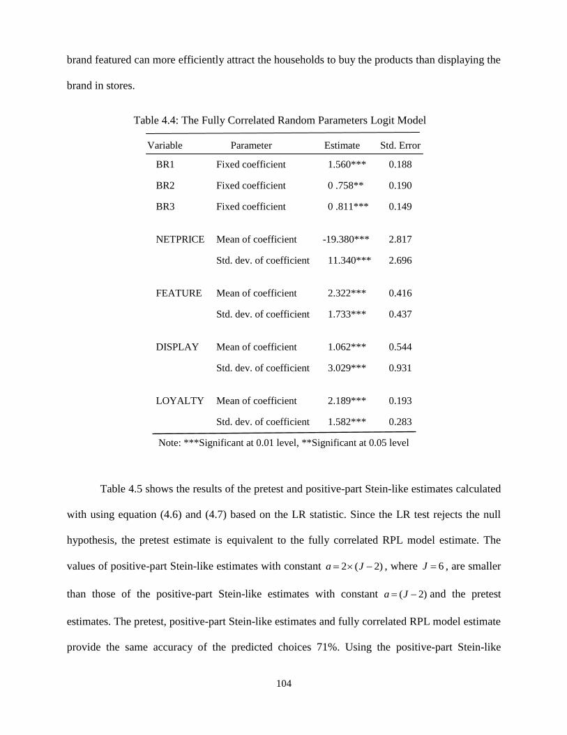
104

brand featured can more efficiently attract the households to buy the products than displaying the

brand in stores.

Table 4.4: The Fully Correlated Random Parameters Logit Model

Variable Parameter Estimate Std. Error

BR1 Fixed coefficient 1.560*** 0.188

BR2 Fixed coefficient 0 .758** 0.190

BR3 Fixed coefficient 0 .811*** 0.149

NETPRICE Mean of coefficient -19.380*** 2.817

Std. dev. of coefficient 11.340*** 2.696

FEATURE Mean of coefficient 2.322*** 0.416


DISPLAY Mean of coefficient 1.062*** 0.544


LOYALTY Mean of coefficient 2.189*** 0.193


Note: ***Significant at 0.01 level, **Significant at 0.05 level

Table 4.5 shows the results of the pretest and positive-part Stein-like estimates calculated

with using equation (4.6) and (4.7) based on the LR statistic. Since the LR test rejects the null

hypothesis, the pretest estimate is equivalent to the fully correlated RPL model estimate. The

values of positive-part Stein-like estimates with constant 2 ( 2)a J , where 6J , are smaller

than those of the positive-part Stein-like estimates with constant ( 2)a J and the pretest

estimates. The pretest, positive-part Stein-like estimates and fully correlated RPL model estimate

provide the same accuracy of the predicted choices 71%. Using the positive-part Stein-like

105

estimate with constant 2 ( 2)a J improve the accuracy of the predicted choices by around

2%. Even though there is not too much difference between the fully correlated RPL model

estimate and the positive-part Stein-like estimates, the shrinkage estimation still can improve the

accuracy of the predicted choices. It also implies that applying uncorrelated RPL model

estimates may provide more slightly accurate predicted choices than using fully correlated RPL

model estimates. However, it will not provide the correlation information of the random

coefficients which is sometimes important for the policy-makers.

Table 4.5: Parameter Estimates for the Fully Correlated Random Parameters Logit Model

Variable Parameter Pretest Stein1 Stein2

BR1 Fixed coefficient 1.560 1.513 1.505



NETPRICE Mean of coefficient -19.380 -18.744 -18.635

Std. dev. of coefficient 11.340 11.575 11.811

FEATURE Mean of coefficient 2.322 2.182 2.158


DISPLAY Mean of coefficient 1.062 1.043 1.039


LOYALTY Mean of coefficient 2.189 2.224 2.231


Accuracy of the Predicted Choices 0.714 0.714 0.732

Note: Stein1 with constant ( 2)a J and Stein2 with constant 2( 2)a J

106

4.6 Conclusions

According to our Monte Carlo experiment results, the uncorrelated RPL model estimators have

smaller estimation risk than the fully correlated RPL model estimators. The positive-part Stein-

like estimators with higher constant a outperform those with a smaller a and it also

outperformances the pretest estimators. The pretest and positive-part Stein-like estimators both

perform better than the fully correlated RPL model estimators. With the marketing consumer

choice data, the positive-part Stein-like estimator with larger constant a improve the percentage

of correct predicted choices by 2% compared to the results with pretest and fully correlated RPL

model estimates. In our Monte Carlo experiments, the ratios of the MSE of estimated mean and

standard deviation with the uncorrelated RPL model to those with the fully correlated RPL

model close to one when the correlation between the random coefficients is closer to one. Using

the shrinkage estimation can reduce the risk of the fully correlated RPL model estimator by

shrinking the fully correlated RPL model estimate towards the uncorrelated RPL model estimate

and improve the percentage of correct predicted choices.

107

CHAPTER 5 CONCLUSION

As a generalization of the conditional logit model, the random parameters logit model does not

impose the Independence from Irrelevant Alternatives (IIA) assumption and the unobserved

factors of utility are not limited to the normal distribution and can be correlated over time. The

random parameters logit model has become popular and is used in marketing, transportation,

labor market and political science research. However, there are few studies analyzing the

efficiency of the random parameters logit model estimators and testing the random parameters in

the random parameters logit model.

This dissertation uses the quasi-Monte Carlo experiments to study the properties of the

pretest and positive-part Stein-like estimators in the random parameters logit model. We explore

the power of the likelihood ratio, Lagrange multiplier and Wald tests for testing the random

parameters in the RPL model, using the conditional logit model as the restricted model. Even

though the RPL model is a very flexible model, its disadvantage is that the related choice

probability cannot be calculated exactly, because it involves a multi-dimensional integral which

does not have closed form. The use of pseudo-random numbers to approximate the integral

during the simulation requires a large number of draws and leads to long computational times.

With pseudo-random numbers, to make the simulated log-likelihood function asymptotically

equivalent to the log-likelihood function on the exact probabilities, the number of draws should

rise faster than the square root of the sample size (Hajivassiliou and Ruud, 1994; McFadden and

Train, 2000). To reduce the huge computational time, in our Monte Carlo experiments, the quasi-

random numbers generated by Halton sequences are used to replace the pseudo-random

numbers. To study the asymptotic properties of the maximum simulated likelihood estimator

with using the quasi-random numbers, we vary the number Halton draws, the sample size and the

number of random coefficients. We find that increases in the number of Halton draws influence

108

the efficiency of the random parameters logit model estimators only slightly. The maximum

simulated likelihood estimator is consistent. These results are also true for the correlated random

coefficients cases, since the correlated distribution can be transformed into independent ones by

using Cholesky decomposition. Our results provide the guide of how to choose the Halton

numbers in the random parameters logit model estimation.

In the third chapter, the pretest estimation in the random parameters logit model is

constructed based on the likelihood ratio, Lagrange multiplier and Wald tests, using the

conditional logit model as the restricted model. The poor risk properties of the LM-based pretest

estimator make us to explore the power of the LR, LM and Wald tests for testing the random

coefficients in the random parameters logit model. After calculating the empirical 90th and 95th

percentile values of the LR, LM and Wald test statistic distributions, we examine rejection rates

by using the empirical 90th and 95th percentile values as the critical values for 10% and 5%

significance level. We find that the power of LR and Wald tests decreases with increases in the

mean of the coefficient distribution. The results of power of these three tests are essentially

consistent with the results of the related pretest estimation. The weak power of the LM test for

the presence of the random coefficient is caused by the failure of taking into account the

properties of the one-tailed alternative hypothesis. Even though the Kuhn-Tucker multiplier test

adjusts the estimated Lagrange multipliers to make the test asymptotically equivalent to the LR

and Wald tests, computing the Kuhn-Tucker multiplier test is complicated. This chapter raises

the issue of how to testing the random coefficients in the random parameters logit model,

especially when the number of the random coefficients is greater than three. Not just in the non-

linear case, this problem also happens in the linear model, such as how to test the individual and

time effects in the random effect model. Since the dimension of the random coefficients can be

high, testing the random coefficients becomes very difficult. However, with more and more

109

applications of the random parameters logit model, how to test the random coefficients become

very important and will be our future research.

The last contribution of this dissertation is exploring the risk properties of the pretest and

positive-part Stein-like estimators in the fully correlated random parameters logit model, using

the mean squared error of estimation as the risk function. The positive-part Stein-like estimators

with higher shrinkage constant a outperform those with less shrinkage and the pretest

estimators. The pretest and positive-part Stein-like estimators both perform better than the fully

correlated RPL model estimators. The average relative losses of the pretest and shrinkage

estimators compared to that of the fully correlated RPL model estimator are significantly less

than one at 0.05 significance level. The average relative losses of the shrinkage estimators are

significantly less than those of the pretest estimator at 0.05 significance level. Even though the

positive-part Stein-like estimators improve the predictive probability only 2% in the marketing

example we considered, it doesn’t mean that the positive-part Stein-like estimators will not

improve the accuracy of predictive probability greatly with other data. It also confirm the

statement of Hensher and Greene (2001) that the high quality data is required if the analyst want

to take advantage of this advanced discrete choice model.

110

REFERENCES

Adkins, L.C. and Hill, R.C. (1989). Risk characteristics of a Stein-like estimator for the probit

regression model, Economics Letters, 30, 19-26

Ahmed, S. Ejaz, and Nicol Christopher (2010). An application of shrinkage estimation to the

nonlinear regression model, Computational Statistics and Data Analysis

Aitchison, J. and Silvey, S. D. (1958). Maximum likelihood estimation of parameters subject to

restraints. Annals of Mathematical Statistics, Vol. 29, 813-828

Andrews, Donald W. K. (2001). Testing when a parameter is on the boundary of the maintained

hypothesis. Econometrica, Vol 69, No.3, 683-734

Bhat, C. R., (2001). Quasi-random maximum simulated likelihood estimation of the mixed

multinomial Logit model. Transportation Research PartB, 35(7), 677-693

Bhat, C. R., (2003). Simulation estimation of mixed discrete choice models using randomized

and scrambles Halton sequences. Transportation Research PartB, 37(9), 837-855

Boyd, J. and Mellman, J., (1980). The effect of fuel economy standards on the U.S. automotive

market: A hedonic demand analysis, Transportation Research A 14, 367-378

Bratley, P., Fox, B.L. and Niederreiter, H. (1992). Implementation and tests of low-discrepancy

sequences” ACM Transactions on Modeling and Computer Simulation 2, 195-213

Cardell, S. and Dunbar, F., (1980). Measuring the societal impacts of automobile downsizing,

Transportation Research A 14, 423-434

Chang, Jae Bong, and Lusk, Jayson, L. (2011). Mixed logit models: accuracy and software

choice, Journal of Applied Econometrics, Volume 26, Issue 1, 167-172

Fang, K.T. and Wang, Y., (1994). Number-theoretic Methods in Statistics, London: Chapman

and Hall/CRC

Gourieroux, Christian, Holly, Alberto and Monfort, Alain (1982). Likelihood ratio test, Wald

test, and Kuhn-Tucker test in linear models with inequality constraints on the regression

parameters. Econometrica, Vol 50, No. 1, 63-88

Gourieroux, Christian and Monfort, Alain (1995). Statistics and econometric models,

Cambridge: Cambridge University Press

Greene, William H. (2008). Econometric Analysis, New Jersey: Pearson Education, Inc.

Guadagin, Peter M. and John D. Little (1983). A logit model of brand choice calibrated on

scanner data, Marketing Science, 2 (Summer), 203-238

Hajivassiliou, V. and P. Ruud. (1994). Classical estimation methods for LDV models using

simulation. Handbook of Econometrics, eds. R. Engle and D. McFadden, vol. IV,

2383–2441. Amsterdam: North-Holland.

111

Halton, J. H., (1960). On the efficiency of certain quasi-random sequences of points in

evaluating multi-dimensional integrals. Numerishe Mathematik 2, 84-90

Hensher, D., & Greene, W. (2003). The mixed logit model: The state of practice, Transportation,

30(2), 133-176

Judge, G.G. and M.E. Bock (1978). The Statistical Implications of Pre-test and Stein-rule

Estimators in Econometrics, North-Holland, Amsterdam

Keng, H.L. and Yan, W., (1981). Application of Number Theory to Numerical Analysis, Spring-

Verlag Berlin Heidelberg New York

Kim, M. and Hill, R. C. (1995). Shrinkage estimation in nonlinear regression: the Box-Cox

transformation, Journal of Econometrics, 66, 1-33

McFadden, Daniel (1974). Conditional Logit analysis of qualitative choice behavior, Frontiers in

Econometrics, Academic Press, New York, 105-142

McFadden, Daniel and Train, Kenneth E. (2000). Mixed MNL models for discrete response,

Journal of Applied Econometrics, 15, 447-470

Morokoff, W.J. and Caflisch, R.E.C., (1995). Quasi-Monte Carlo integration, Journal of

Computational Physics, 122, 218-230

Niederreiter, H., (1992). Random Number Generation and Quasi-Monte Carlo Methods,

Philadelphia: Society for Industrial Mathematics

Ruud, Paul A. (1996). Approximation and simulation of the multinomial probit model: an

analysis of covariance matrix estimation

Train, K. E., (2003). Discrete Choice Methods with Simulation, Cambridge: Cambridge

University Press

Wang, X. Q. and Hickernell, Fred J., (2000). Randomized Halton Sequence, Mathematical and

Computer Modeling 32, 887–899

Yan, S. Y., (2002). Number Theory for Computing, Berlin Heidelberg New York: Springer-

Verlag

Sapra, Sunil K. (1993). Consistent estimation of a limiting covariance matrix, Bulletin of

Economic Research, Volume 45, Issue 2, 161-163

Silvey, S. D. (1959). The Lagrangian multiplier test. Annals of Mathematical Statistics, Vol 30,

389-407

Swamy, P.A.V.B. and Tavlas, G.S. (2001). Random coefficient models, Chap. 19. In: Baltagi,

B.H. (ed.)

112

APPENDIX: THE DISCREPANCY OF HALTON SEQUENCES

Based on the base- p number system, any positive integer n can be written as:

2

1 2 1 0 0 1 2

M

M M Mn n n n n n n n p n p n p

where [log ] [ln / ln ]n

pM n p , square brackets denoting the integral part, p is base and can be

any integer except 1, in is the digit at position i , 0 i M , 0 1in p .

For each positive integer n , we can construct unique fraction by the radical inverse function.

1 2 1

0 1 2 0 1( ) 0. M


To expand to k fractions, setting 1 2, , , kp p p to be prime to each other and

1 2max( , , , )kn p p p ,

then we have:

1 2

( ( ), ( ), , ( ))kp p pn n n

For each fraction ( )ip n , 1 i k , we have:

1

1 2 1

1,0 1,1 1,2 1, 1,0 1,1 1,( ) 0. M


2

1 2 1

2,0 2,1 2,2 2, 2,0 2,1 2,( ) 0. M


1 2 1

,0 ,1 ,2 , ,0 ,1 ,( ) 0.k

M

p k k k k M k k k Mn n n n n n p n p n p

For an arbitrary positive fraction A , 0 1A , which is supposed to be non-terminate, then A is

written as:

0 1 20. MA a a a a

If ( )p n A , one of the following conditions must be satisfied:

(1) 0 0a n

(2) 0 0 1 1,a n a n

113

( M ) 0 0 1 1 2 2 1 1, , , ,M M M Ma n a n a n a n

( 1M ) 0 0 1 1 1 1, , , ,M M M Ma n a n a n a n

( 2M ) 0 0 1 1 1 1, , , ,M M M Ma n a n a n a n

The above conditions can be rewritten in the form of congruence:

(1) 0 (mod )n n p ,

0 00 n a

(2) 2

0 1 (mod )n a n p p , 1 10 n a

( M ) 2 1

0 1 2 1 (mod )M M M

M Mn a a p a p n p p

, 1 10 M Mn a

( 1M ) 1 1

0 1 1 (mod )M M M

M Mn a a p a p n p p

, 0 M Mn a

( 2M ) 1 2

0 1 1 (mod )M M M

M Mn a a p a p a p p

, M Mn a

Lemma 1.1 The number of solutions of the congruence

(mod )x a m , 1 x n

is equal to n m h ,where 1h or 0h

Based on the Lemma 1.1, the numbers of solutions of the above congruence are:

(1) 0 ( )a n p

(2) 2

1( )a n p

( M ) 1( )M

Ma n p

( 1M ) 1

( )M

Ma n p

114

( 2M ) 2

( )M

n p

Where 0 1 , can take different value.

So the total number of n satisfying ( )p n A is:

2 1

0 1( ) ( ) ( )M

Ma n p a n p a n p

Theorem 1.1 (The Chinese Reminder Theorem CRT) If 1 2, , , nm m m are pairwise relatively

prime and greater than 1, and 1 2, , , na a a are any integers, then there is a solution x to the

following simultaneous congruences:

ix a (mod )im

If x and x are two solutions, then (mod )x x M , where 1 2 nM m m m .

Let ( )S A denote the number of integers n in the sequences 1,2, , N satisfying the following

conditions simultaneous:

1( ) ,p n A

2( ) ,p n A , ( )

kp n A

Based on the Lemma 1.1 and Theorem 1.1,

1 2

1 2

11 1

, 11 1 1 1

( ) ( )( )k

i

i

k

MM M km

i m im m m i i

S A b N p

Where ln lni iM N p , 1 2i im M and , ,i m i mb a , but when 2i im M , , 1 1

ii mb , square

brackets denoting the integral part.

Let V represent the volume of hyper-brick defined by the arbitrary point1( , )kA A A , 0 1iA (

1,2, ,i k ). Then 1 2 kV A A A .

Theorem 1.2 The k -dimensional Halton sequences

1 2

( ( ), ( ), ( ))kn p p pn n n

115

generated from base 1 2, , , kp p p ,which are pairwise prime to each other and chosen from the

first k primes, 1,2, ,n N , where 1 2max( , , , )kN p p p , have discrepancy

(ln )k

N k

ND C

N

Proof. [0,1)

sup ( )NA

D S A N V

1 1 1

, 1 , 1 , 11 1 1 1 1 11 1 1 1

i i i

i i i

k k k

k k k km m m

i m i i m i i m im m m m m mi i i i

NV N a p N a p a N p

So 1 2

1 2 1

11 1

, 1 , 11 1 1 1 11 1 1 1

( ) ( )( )k

i i

i i

k k

MM M k k k km m

i m i i m im m m m mi i i i

S A NV b N p a N p

( )S A represent the number of the points, which are generated by the k -dimensional Halton

sequences of length N , falling in the hyper-brick defined by A . If we increase V and keep

( )S A unchanged, the discrepancy ND will increase.

Since

1

1

1 1 1

, 11 1 1 1

11

, 1 , 11 1 2 21 1 1 1

i

i

k

k

i i

i i

k k k

k km

i m im m i i

MM k k k km m

i m i i m im m m M m Mi i i i

a N p

a N p a N p

and

1 1 1 1

, 12 2 2 21 1 1 1

( 1)i i

i

k k k k

k k k km m

i m i i im M m M m M m Mi i i i

a N p p N p

11 1 1 1

11 1i

i

k k k kMi

i i iMi i i ii

pN p p N p

p

We have:

1 2

1 2

11 1

, 11 1 1 1 1 1 1

( )

( ) 1k

i i i

i

k

MM M k k k km m M

i m i i i im m m i i i i i

S A NV

a N p N p p N p

116

1 2

1 2

11 1

, 11 1 1 1 1 1 1

( ) 1k

i i i

i

k

MM M k k k km m M

i m i i i im m m i i i i i

a N p N p p N p

Since 1

0 1i i

km m

i ii i

N p N p

and 1 1

0 1 1i

k kM

i ii i

p N p

Let . ,i m i mc a , except for , , 1i ii M i Mc a , then we have:

1

1

11

, 11 1 1

( )k

i

k

MM k

i mm m i

S A NV c

Since, . ,i m i mc a for 1 i im M , and , , 1i ii M i Mc a , for 1,i im M we can get:

,0 1,ii m ic p

for 1 i im M

,0 ,ii m ic p

for 1i im M

And

1

sup ( ) 1k

i i iA i

S A NV M p p

Since 1 2max( , , , )kN p p p and ln lni i

M N p , then 1 ln lni iM N p and

1 1

2 1lnsup ( ) ( 1) ln

ln ln

k kk i

i iA i ii i

pNS A NV p p N

p p

So

1

2 1( ) (ln ) (ln )sup

ln

k kki

N kA i i

pS A N ND V C

N N p N

The theorem is proved.

Lemma 1.2 Let 2N N and 1 2max( , , , )kN p p p , under the assumption of Theorem 1.2, k -

dimensional Halton sequences 1 2

( ( ), ( ), ( ))kn p p pn n n , where 1,2, ,n N has the

discrepancy:

117

2

(2ln )k

N k

ND C

N

Proof

1 2

1 2 1

11 1

, 1 , 11 1 1 1 11 1 1 1

( ) ( )( )k

i i

i i

k k

LL L k k k kl l

i l i i l il l l l li i i i

S A N V b N p a N p

1 2

1 2

11 1

, 11 1 1 1 1 1 1 1

( ) 1k

i i i

i

k

LL L k k k k kl l L

i l i i i il l l i i i i i

a N p N p p N p

1 2

1 2

11 1

, 11 1 1 1 1 1 1 1

( ) 1k

i i i

i

k

LL L k k k k kl l L

i m i i i il l l i i i i i

a N p N p p N p

1

1

11

, 11 1 1

k

i

k

LL k

i ll l i

c

Where . ,i m i mc a for 1 i il L , and , , 1i ii M i Mc a , for 1i il L

So

1

sup ( ) 1k

i i iA i

S A N V L p p

Since 2N N 1 2max( , , , )kN p p p and ln lni i

L N p , then ln ln ln lnii iN p L N p and

2

1 1

2 1lnsup ( ) ( 1) 2ln

ln ln

k kk i

i iA i ii i

pNS A N V p p N

p p

So we can get:

2 2

1

2 1( ) (2ln ) (2ln )sup

ln

k kki

N kA i i

pS A N ND V C

N N p N

The Lemma is proved.

118

VITA

Tong Zeng obtained her Bachelor of Economics degree in 1999 from Wuhan University. After

several years working experience in industry, she came to the United States to pursue a doctoral

degree at Louisiana State University in August 2005. She received her Master of Science degree

in economics from Louisiana State University in 2007. She expects to obtain her Doctor of

Philosophy in economics with a concentration in econometrics at December in 2011.

essays on the random parameters logit model

Documents