essays on individual and institutional willingness to take
TRANSCRIPT

Essays on Individual andInstitutional Willingness to Take
Risks
Cumulative Dissertation
Submitted to the
Faculty of Business Administration
of the University of Hamburg
in partial fulfillment of the requirements for the degree of
Doctor rerum oeconomicarum
Submitted by
Diplom-Volkswirt Roger Gothmann
from Hagenow
Hamburg
February 13, 2019

Chair of Dissertation Committee:
Prof. Dr. Nicola Berg, Faculty of Business Administration, University of Hamburg
First Reviewer:
Prof. Dr. Markus Noth, Faculty of Business Administration, University of Hamburg
Second Reviewer:
Prof. Dr. Kay Peters, Faculty of Business Administration, University of Hamburg

Contents
List of Tables III
List of Figures IV
1 General Introduction 11.1 Object of Study . . . . . . . . . . . . . . . . . . . . . . . . . . . . . . . . . 21.2 Overview and Summary of Chapters . . . . . . . . . . . . . . . . . . . . . 41.3 Summary . . . . . . . . . . . . . . . . . . . . . . . . . . . . . . . . . . . . 9References . . . . . . . . . . . . . . . . . . . . . . . . . . . . . . . . . . . . . . . 11
2 Risk Taking and Induced Reference Points 132.1 Introduction . . . . . . . . . . . . . . . . . . . . . . . . . . . . . . . . . . . 142.2 Design . . . . . . . . . . . . . . . . . . . . . . . . . . . . . . . . . . . . . . 17
2.2.1 Additional Measures . . . . . . . . . . . . . . . . . . . . . . . . . . 212.2.2 Execution . . . . . . . . . . . . . . . . . . . . . . . . . . . . . . . . 22
2.3 Theories and Predictions . . . . . . . . . . . . . . . . . . . . . . . . . . . . 222.3.1 Expected Utility Theory . . . . . . . . . . . . . . . . . . . . . . . . 222.3.2 Expected Utility Alternatives . . . . . . . . . . . . . . . . . . . . . 23
2.4 Results . . . . . . . . . . . . . . . . . . . . . . . . . . . . . . . . . . . . . . 272.4.1 Descriptive Results . . . . . . . . . . . . . . . . . . . . . . . . . . . 272.4.2 Model Estimation and Selection - Specifying the Reference Point . . 302.4.3 Robustness Checks . . . . . . . . . . . . . . . . . . . . . . . . . . . 36
2.5 Conclusion . . . . . . . . . . . . . . . . . . . . . . . . . . . . . . . . . . . . 38References . . . . . . . . . . . . . . . . . . . . . . . . . . . . . . . . . . . . . . . 39
3 Risk Taking and Compensation Schemes 433.1 Introduction . . . . . . . . . . . . . . . . . . . . . . . . . . . . . . . . . . . 443.2 Institutional Overview . . . . . . . . . . . . . . . . . . . . . . . . . . . . . 46
3.2.1 Legal Framework . . . . . . . . . . . . . . . . . . . . . . . . . . . . 463.2.2 Empirics . . . . . . . . . . . . . . . . . . . . . . . . . . . . . . . . . 47
3.3 Literature . . . . . . . . . . . . . . . . . . . . . . . . . . . . . . . . . . . . 503.4 Theoretical Predictions and Hypotheses . . . . . . . . . . . . . . . . . . . . 513.5 Experimental Design . . . . . . . . . . . . . . . . . . . . . . . . . . . . . . 553.6 Results . . . . . . . . . . . . . . . . . . . . . . . . . . . . . . . . . . . . . . 59
3.6.1 Descriptive Results . . . . . . . . . . . . . . . . . . . . . . . . . . . 593.6.2 Robustness Checks . . . . . . . . . . . . . . . . . . . . . . . . . . . 63
3.7 Conclusion . . . . . . . . . . . . . . . . . . . . . . . . . . . . . . . . . . . . 63References . . . . . . . . . . . . . . . . . . . . . . . . . . . . . . . . . . . . . . . 65
I

CONTENTS II
4 Asset Management of German Foundations 684.1 Introduction . . . . . . . . . . . . . . . . . . . . . . . . . . . . . . . . . . . 694.2 Institutional (Legal) Framework . . . . . . . . . . . . . . . . . . . . . . . . 71
4.2.1 German Foundation Law . . . . . . . . . . . . . . . . . . . . . . . . 714.2.2 Current Jurisdiction . . . . . . . . . . . . . . . . . . . . . . . . . . 774.2.3 Summary of Relevant Legal Restrictions . . . . . . . . . . . . . . . 80
4.3 Financial Framework . . . . . . . . . . . . . . . . . . . . . . . . . . . . . . 804.3.1 Empirics . . . . . . . . . . . . . . . . . . . . . . . . . . . . . . . . . 814.3.2 Literature – Asset Management for (German) Foundations . . . . . 844.3.3 Performance and Risk Measures - Foundation Utility Optimization 864.3.4 Potential Asset Classes . . . . . . . . . . . . . . . . . . . . . . . . . 874.3.5 Target Return and Interest Rates . . . . . . . . . . . . . . . . . . . 914.3.6 Diversification Strategies . . . . . . . . . . . . . . . . . . . . . . . . 92
4.4 Quantitative Analysis . . . . . . . . . . . . . . . . . . . . . . . . . . . . . . 954.4.1 Simulation Method and Design . . . . . . . . . . . . . . . . . . . . 954.4.2 Markowitz Optimization - Minimum Variance . . . . . . . . . . . . 974.4.3 Heuristics . . . . . . . . . . . . . . . . . . . . . . . . . . . . . . . . 98
4.5 Simulation Results . . . . . . . . . . . . . . . . . . . . . . . . . . . . . . . 984.5.1 Basic Scenario . . . . . . . . . . . . . . . . . . . . . . . . . . . . . . 984.5.2 Benchmark Portfolio(s) . . . . . . . . . . . . . . . . . . . . . . . . . 984.5.3 Minimum Variance Portfolio . . . . . . . . . . . . . . . . . . . . . . 994.5.4 Heuristics - Euro Investments . . . . . . . . . . . . . . . . . . . . . 1004.5.5 Heuristics - GDP-Weighted Stocks . . . . . . . . . . . . . . . . . . 1004.5.6 Heuristics - Equally-Weighted Stocks . . . . . . . . . . . . . . . . . 1004.5.7 Commodities . . . . . . . . . . . . . . . . . . . . . . . . . . . . . . 1044.5.8 Welfare Losses . . . . . . . . . . . . . . . . . . . . . . . . . . . . . . 1054.5.9 Results - Subscenarios . . . . . . . . . . . . . . . . . . . . . . . . . 107
4.6 Conclusion . . . . . . . . . . . . . . . . . . . . . . . . . . . . . . . . . . . . 113References . . . . . . . . . . . . . . . . . . . . . . . . . . . . . . . . . . . . . . . 114
A Appendices iA.1 Appendix – Induced Expectations and Risk Taking . . . . . . . . . . . . . ii
A.1.1 Regression Results . . . . . . . . . . . . . . . . . . . . . . . . . . . iiA.1.2 Appendix – Induced Expectations and Risk Taking (Experiment
Documentation) . . . . . . . . . . . . . . . . . . . . . . . . . . . . . ivA.2 Appendix – Risk Taking and Compensation Schemes (Experiment Docu-
mentation) . . . . . . . . . . . . . . . . . . . . . . . . . . . . . . . . . . . . xxiiA.3 Appendix – Asset Management of German Foundations . . . . . . . . . . . xxxii
A.3.1 Regulatory Main Principles for German Foundations . . . . . . . . xxxiiA.3.2 German Translation of Table 4.1 . . . . . . . . . . . . . . . . . . . xxxiiiA.3.3 Extracts from Federal State Foundation Laws . . . . . . . . . . . . xxxiv
B General Appendix xlB.1 Abstracts and Current Status of Papers (§6 (5) PromO) . . . . . . . . . . xliB.2 Statement of Personal Contribution (§6 (3) PromO) . . . . . . . . . . . . . xlivB.3 Affidavit (§6 (4) PromO) . . . . . . . . . . . . . . . . . . . . . . . . . . . . xlv

List of Tables
1.1 Titles and Topics of Essays . . . . . . . . . . . . . . . . . . . . . . . . . 4
2.1 Modified HL-lotteries . . . . . . . . . . . . . . . . . . . . . . . . . . . . . 202.2 Risk Aversion Classifications . . . . . . . . . . . . . . . . . . . . . . . . . 212.3 Descriptive Results — RP-Susceptives . . . . . . . . . . . . . . . . . . . 302.4 Descriptive Results — NON-RP-Susceptives . . . . . . . . . . . . . . . . 302.5 Maximum Likelihood Estimates: Expected Utility (CRRA) . . . . . . . . 322.6 Maximum Likelihood Estimates: Rank Dependence (Quiggin 1982) . . . 342.7 Maximum Likelihood Estimates: Disappointment Aversion . . . . . . . . 352.8 Model Selection HL-lotteries . . . . . . . . . . . . . . . . . . . . . . . . . 352.9 Model Selection MHL-lotteries . . . . . . . . . . . . . . . . . . . . . . . . 36
3.1 Experiment: EUT - Predictions . . . . . . . . . . . . . . . . . . . . . . . 533.2 Ranking of Possible Outcomes According to Disappointment Aversion . . 553.3 Experiment: Multiple Price List . . . . . . . . . . . . . . . . . . . . . . . 573.4 HL Lotteries . . . . . . . . . . . . . . . . . . . . . . . . . . . . . . . . . 583.5 Degree of Risk Aversion . . . . . . . . . . . . . . . . . . . . . . . . . . . 62
4.1 Preservation Principles of the German Federal States . . . . . . . . . . . 744.2 Legal Classification of Foundation Assets . . . . . . . . . . . . . . . . . . 774.3 German Court Decisions Regarding the Asset Management of German
Foundations . . . . . . . . . . . . . . . . . . . . . . . . . . . . . . . . . . 794.4 Asset Classes Suggested for Private Investors . . . . . . . . . . . . . . . 884.5 Overview: Time Series, 2003 –2012 . . . . . . . . . . . . . . . . . . . . . 904.6 Descriptive Statistics for Asset Classes to be Considered (Estimation
Period: 2003–2012). . . . . . . . . . . . . . . . . . . . . . . . . . . . . . 904.7 Diversification Approaches . . . . . . . . . . . . . . . . . . . . . . . . . . 944.8 Weights of the Minimum Variance Portfolio . . . . . . . . . . . . . . . . 984.9 Results of the Benchmark-Portfolio (after one and five years) . . . . . . . 994.10 Results of the MV-Portfolio (after one and five years) . . . . . . . . . . . 994.11 Results Euro Investments (five years) . . . . . . . . . . . . . . . . . . . . 1014.12 Results GDP-Weighted Stock Components (five years) . . . . . . . . . . 1024.13 Results 1
N-Weighted Stock Components (five years) . . . . . . . . . . . . 103
4.14 Results GDP-Weighted Stocks and Commodities (five years) . . . . . . . 1044.15 Choice Behavior and Welfare Losses . . . . . . . . . . . . . . . . . . . . 1064.16 Results of the Benchmark-Portfolio (after five years) . . . . . . . . . . . 1074.17 Results of the MV-Portfolio (after five years) . . . . . . . . . . . . . . . . 1084.18 Results of Euro-Investments (after five years) . . . . . . . . . . . . . . . 1104.19 Results of GDP-heuristic (after five years) . . . . . . . . . . . . . . . . . 1114.20 Choice Behavior and Welfare Losses . . . . . . . . . . . . . . . . . . . . 112
A.1 Preservation Principles of the German Federal States . . . . . . . . . . . xxxiii
III

List of Figures
2.1 Modified HL-lotteries (MHL) . . . . . . . . . . . . . . . . . . . . . . . . 192.1 Cumulated Fraction of Safe Choices — HL + MHL all subjects . . . . . 282.2 Cumulated Fraction of Safe Choices — HL+ MHL RP-Susceptives . . . . 292.3 Control Task — HL-lotteries with 10 Draws . . . . . . . . . . . . . . . . 37
3.1 Variable Remuneration for Identified Staff 2014 . . . . . . . . . . . . . . 483.2 Variable Cash Component and Ratio of Fixed and Variable Remuneration
for Identified Staff (2010 - 2014) . . . . . . . . . . . . . . . . . . . . . . . 493.3 Results: DA-Induced Risk Taking . . . . . . . . . . . . . . . . . . . . . . 603.4 Results: Mere Risk Preferences . . . . . . . . . . . . . . . . . . . . . . . 613.5 Results: DA-Induced Risk Taking vs. Mere Risk Taking . . . . . . . . . 63
4.1 German Foundation Properties in Classes . . . . . . . . . . . . . . . . . 814.2 Distribution of Asset Classes 2005 Heissmann (2005) . . . . . . . . . . . 824.3 Distribution of Asset Classes 2009 BVDS (2010) . . . . . . . . . . . . . . 834.4 Pearson Correlation of Relevant Assets . . . . . . . . . . . . . . . . . . . 914.5 Interest Rates, Price and Wage Inflation – 2003 - 2012 . . . . . . . . . . 924.6 Basic (2003 - 2012) - and Subscenarios (2002 - 2007 and 2008 - 2012) . . 974.7 Results Euro-Investments (five years) . . . . . . . . . . . . . . . . . . . . 1014.8 Results GDP-Weighted Stocks Components (five years) . . . . . . . . . . 1024.9 Results 1
N-Weighted Stocks Components (five years) . . . . . . . . . . . . 103
IV

Chapter 1
General Introduction
1

CHAPTER 1. GENERAL INTRODUCTION 2
1.1 Object of Study
Starting with the work of Jensen and Meckling (1976), the question how risk preferences
of agents (i.e, managers) can be aligned with the risk appetite of principals (i.e., equity
providers) has become an important question in economic research.
The welfare losses incurred by excessive risk taking in the financial industry before the
financial crisis are hard to quantify in accordance with scientific and economic principles.
Nevertheless, this event has once again drawn the attention of research and politics to one
of the underlying reasons, the principal agent dilemma.
The common theme of this thesis, which consists of three essays, is individual decision
making under risk and uncertainty.1
All essays address a major legal and economic problem: What kind of regulation is
needed in order to neither provide incentives for excessive risk taking nor for absolute risk
avoidance? I provide analytical and empirical evidence for both extremes and its effects on
risk taking. In doing so, I focus on the risk preferences and choice behavior of managers
working for two different kinds of institutions that, as major investors, both have significant
influence on economic welfare: financial institutions and non-profit foundations.
In order to develop regulatory frameworks for risk taking in sensitive areas such as the
financial industry, one has to understand the mechanisms of individual decision making
under risk.
Neoclassical theory, i.e., Expected Utility Theory (EUT), suggests that the willingness
to take risks is determined by an individual degree of risk aversion and probability-weighted
potential outcomes (Von Neumann and Morgenstern (1947)). However, there is evidence
that individuals tend to adapt their risk preferences to a (desirable) reference point. In
this context, losses loom larger than equal-sized gains, which implies that agents will take
more risk when they fall short of this kind of behavioral anchor and perceive less additional
utility once they have exceeded their reference point. This behavioral pattern was first
described by Allais (1953). Kahneman and Tversky (1979) and Tversky and Kahneman
(1992) (KT) provide a model of reference-dependent preferences which can formalize this
phenomenon: Prospect Theory (PT).
1Risk is characterized by a given set of potential, more or less preferred outcomes plus the availabilityof corresponding outcome probabilities. Whereas, situations in which a decision maker has an incompleteset of potential outcomes and/or no objectively estimable probabilities, can be described as uncertainty(Knight (1921)).
CHAPTER 1. GENERAL INTRODUCTION 3
How to determine someone’s reference point is still a key question in PT. For KT, the
status quo is a candidate for the reference point. Motivated by the findings of Camerer
et al. (1997) that the labor supply of New York Cab drivers is determined by an individual
(daily) income target, Koszegi and Rabin (2006) suggest that expectations can determine
the reference point. Abeler et al. (2011) conduct a laboratory experiment and provide
evidence in favor of this hypothesis. In my first essay (Chapter 2), I aim to transfer this
finding from labor supply to risk taking. The result presented in this essay is important,
because as far as there is no validated concept, reference-dependent models still have the
drawback of an additional degree of freedom. This implies less predictive power than
standard EUT-models. Chapter 3 studies whether regulatory constraints on executive
compensation schemes in the aftermath of the financial crisis (i.e., bonus caps) have an
effect on risk taking. In doing so, I transfer my results of Chapter 2 in order to examine
the initial question: How can risk preferences of principals and agents be aligned?
The first two essays (Chapter 2 and 3) present empirical analyses of experiments.
This method provides a maximum degree of control. Experiments also allow for causal
interpretations since effects (i.e., treatments) can be assigned exogenously. Chapter 4
studies risk taking of German foundation managers by means of empirical and stochastic
analyses. Whereas the possible failure of financial institutions and its economic costs due
to excessive risk taking of managers is in the focus of public attention (e.g., Reinhart and
Rogoff (2009)), German foundations and their influence on economic welfare have so far
not been subject to similar investigations so far. As I will show, this sector is, similar to
the financial industry, also highly regulated. Therefore, the underlying research question,
in comparison with Chapter 3, is the same: What is the effect of legal constraints on
individual risk taking?
Table 1.1 illustrates the topics of all three essays.

CHAPTER 1. GENERAL INTRODUCTION 4
Table 1.1: Titles and Topics of Essays
Chapter Title – Author(s) Topic
2 Risk Taking and Induced Refer-ence Points – Roger Gothmann andMarkus Noth
Identification of Mechanisms ofReference-Dependent Preferencesunder Risk
3 Risk Taking and Compensation –Roger Gothmann
Effects of the Remuneration Struc-ture of Executives on Individual Will-ingness to Take Risks
4 Asset Management of German Foun-dations – Roger Gothmann
Asset Management under Regula-tory Restrictions for German Non-Profit Foundations
Notes: List of essays according to §6 (2) Promotionsordnung 2010, for a detailed overviewof personal contributions (§6 (3) Promotionsordnung 2010) see the General Appendix.
1.2 Overview and Summary of Chapters
This dissertation consists of three independent chapters. All chapters discuss individual
risk taking in different areas and can be read independently of each other.
Expectations and the Willingness to Take Risks (Chapter 2)
In Chapter 2 we test whether expectations can influence individual willingness to take risks
and to what extent. Reference-dependent preferences predict that individuals evaluate
changes in income compared to a reference point whereas EUT takes the level of income as
benchmark.
The theory of reference-dependent preferences (RDP) was initially established in
economics by KT. However, the key question is still open: What determines the reference
point? Without a sound theory, RDPs have an inherent additional degree of freedom. For
their studies, Kahneman and Tversky (1979) work with the status quo. In a subordinate
clause of their last section, KT suggest that expectations could also be a candidate for the
reference point. Koszegi and Rabin (2006) adopt this idea. By doing so, the authors are
able to explain the Cab-Driver-Puzzle mentioned before.
The following example illustrates the difference between status quo and expectations:

CHAPTER 1. GENERAL INTRODUCTION 5
A cash bonus of 50,000 euros at the end of the year is a gain in comparison to the status
quo. However, it can be perceived as a loss if the expected bonus was 100,000 euros.
Abeler et al. (2011) are the first to investigate this hypothesis, using an experiment,
and to find confirming evidence. Their main result is that individuals who expect to earn
more than a control group, work, on average, more than this group. The authors argue
that, with a reference point determined by expectations, subjects work more in order to
avoid disappointment by closing the gap between expected and actual earnings, which is
the definition of loss aversion as the fundamental mechanism of RDP.
In this chapter, we take up the issue raised by Abeler et al. (2011) that the mechanism
how expectations affect reference point formation requires further research. In particular
two strands of literature about reference point formation suggest different candidates: the
highest outcome (e.g., Gul (1991)) or a weighted average (e.g., Quiggin (1982)).
To the best of our knowledge, we are the first to transfer the experimental design
of Abeler et al. (2011) from the field of labor economics (i.e., the provision of effort) to
the topic of risk taking. By means of an online experiment, we test the hypothesis that
potential outcomes of different options are ranked in relation to the best (e.g., highest)
outcome as suggested, for instance, by Gul (1991).
For this purpose, we use a well-established measure for individual risk preferences as
suggested by Holt and Laury (2002) (HL-lotteries) in the first task of our experiment in
order to measure mere risk preferences. Subjects have to choose between a low-risk lottery,
Option A, and a high-risk lottery, Option B, in a series of ten decision tasks. For each task,
the possible outcomes of the lotteries are fixed and identical. Only the probability weights
change from task to task, starting with a weight of 0.1 on the higher outcomes of A (2.0)
and B (3.85) and ending with a weight of 1 in the tenth stage. The lower outcomes of A
and B are 1.6 and 0.1. Thus, a risk-neutral decision maker would start choosing Option
A (low risk) for the first four stages and switch to Option B (high risk) in the fifth stage
when the expected value for Option B is greater than the expected value for Option A
from this stage on. In a second task, subjects have to play the HL-lotteries again. They
receive the outcome of the chosen option only with 50 percent probability. With 50 percent
probability they receive a fixed amount of 3.5. EUT, and RDP with the status quo as
reference point would predict no different risk taking behavior.
In addition, we estimate different RDP-models by running Maximum-Likelihood-
CHAPTER 1. GENERAL INTRODUCTION 6
Estimations on the data in order to answer the question: Is the highest outcome a
possible reference point?
The main findings of our study are as follows: First, we find a significant effect between
both tasks. Individuals switch one stage later from Option A to Option B when they have
the additional chance to receive a higher outcome - the fixed amount. This means that,
according to the scale suggested by Holt and Laury (2002), subjects switch from being
slightly risk averse to being risk neutral. Second, our Maximum-Likelihood estimations
provide evidence for the hypothesis that individuals rank potential outcomes in relation to
the highest outcome in a risk taking framework.
Regarding the design of compensation schemes in the financial sector, our findings are
relevant for the debate how to avoid providing incentives for excessive risk taking.
Risk Taking and Regulation (Chapter 3)
Chapter 3 focuses on the regulation of payment schemes in the financial sector. Managers
of financial institutions had partially taken excessive risks before the financial crisis due to
misdirected compensation schemes, which led to huge welfare losses (e.g., Bebchuk and
Fried (2009)).
In this chapter, I study the effect of capped bonus payments for certain groups of
financial managers (i.e., identified staff 2) to a maximum of 200 percent of their fixed
salary. This constraint was introduced by the European Union3 in the aftermath of the
financial crisis. I empirically analyze the effect of this event on the compensation structure
of European banks. As I am able to show, these institutions increase the fixed salary of
their managers. Chapter 3 focuses on this regulatory arbitrage. In line with this finding,
I use an experiment to analyze this empirical shift in fixed and variable components of
managerial remuneration.
In recent years, a growing body of literature has shown that an optimal CEO compen-
sation should take behavioral aspects and in particular loss aversion into account (e.g.,
Dittmann et al. (2010)). Cole et al. (2015) show in a field experiment with commercial
bank loan officers that monetary incentives such as performance-oriented payments can
bias the assessment of credit risks. However, there is still limited knowledge about the
2Definition: Group of managers who have a profound influence on an institute’s risk profile (Directive2013/36/EU).
3Directive 2013/36/EU
CHAPTER 1. GENERAL INTRODUCTION 7
influence of short-term variable bonus payments on individual willingness to take risks.
I conduct an online experiment in order to examine the effect of the ratio of short-term
bonus payments to fixed salary. Individuals have to decide between a constantly low
variance lottery (Option A) and a constantly high variance lottery (Option B) for each
stage of a setup of 20 decisions tasks. The only variable parameter for all tasks is a fixed
amount (fixed salary) which is the same for every stage of Option A and Option B and
which increases from 6 euros to 25 euros in steps of one euro in order to study whether
an increasing ratio of fixed versus variable compensation has an influence on risk taking.
Both options have the same expected value for each stage. Option B has a considerable
higher variance than Option A. Thus, risk (excessive) taking is defined as switching from
Option A to Option B.
Here is what the data tells us: Given a certain amount of total compensation, a higher
fixed salary can lead to increased (i.e., excessive) risk taking. This behavior can not be
explained by EUT. RDP with a reference point in the highest potential outcome, as I show
in Chapter 2, can provide an explanation: An increased fixed salary can induce a change
of the ranks of potential outcomes. This change of ranks can make the potential outcomes
of the higher variance lottery more desirable.
My main finding is that people tend to take on higher risks when the proportion of
their fixed salary is higher. Aspects, such as reference dependent preferences should be
taken into account. A solution to this problem could be a more heuristical approach by the
legislator as suggested, for instance, by Admati and Hellwig (2014) or Neth et al. (2014),
by ”fixing banker’s pay” which would not allow much leeway for regulatory arbitrage.
Asset Management of German Foundations (Chapter 4)
’A man should always place his money, one-third into land, a third into merchandise and
keep a third in hand ’ (Babylonian Talmud4)
In Chapter 4 of this thesis, I analyze investment decisions of German non-profit
foundation managers who are faced with the following trade-off: the permanent preservation
4See, for instance, Mayer (1963).

CHAPTER 1. GENERAL INTRODUCTION 8
of the foundation’s pool of assets (in real terms) and the generation of sufficient returns
in order to fulfill the foundation’s goals. I address the following questions: What is
the legal (i.e., regulatory) and financial framework for the asset management of German
foundations? Given this institutional framework, what are suitable asset management
strategies? Compared to an empirical benchmark, are there any welfare losses caused by
the investment behavior of German foundation managers?
To the best of my knowledge, this study is the first that combines an analysis of German
foundation law with a study of asset management strategies. By doing so, I extend the
literature on asset management for German foundations which, so far, largely consists of
the work of Schroder (2010).
Therefore, I define a legal framework based on the relevant regulatory restrictions of the
German foundation law. By means of stochastic simulations, I specify and test different
asset management strategies that comply with the legal framework. This part of my third
essay is based on several studies of asset management strategies which provide evidence that
highly sophisticated portfolio optimization strategies with a focus on short-term efficiency
are inferior to simple (but robust) heuristics (e.g., DeMiguel et al. (2009), Jacobs et al.
(2014)).5
For this purpose, I compare empirical asset allocations of German foundations, which
mainly consist of 80 - 90 percent European bonds and 10 - 20 percent European stocks
with (inter alia) GDP-weighted asset allocations as suggested by Jacobs et al. (2014) by
means of Monte-Carlo-simulations. As a main result, I am able to show show that this
heuristic can provide superior results: The probability of preserving the pool of assets in
real terms increases significantly in contrast to decreasing risk measures. By doing so, I
can also quantify welfare losses of empiric asset allocations of German foundations due to
regulatory rules, that sanction a wide range of risk taking.
Regarding the regulation of German foundations, I provide insights in the correlation of
regulatory framework and risk taking. Exaggerated risk awareness of German foundation
managers, induced by a biased jurisdiction which solely sanctions downside risks, can lead
to welfare losses. For this reason, I suggest to simplify the regulatory framework.
The trade-off mentioned above is currently captured by regulatory rules that require
the preservation of assets. In addition, a foundation manager has to spend two-thirds of
5A prominent representative of these heuristics is the 1N -rule which had already been mentioned in the
Talmud centuries ago.

CHAPTER 1. GENERAL INTRODUCTION 9
current yields. Given these rules, one can explain empirical asset allocations that are on
average dominated by highly rated government and corporate bonds. This contradicts
the basic purpose of a (German) non-profit foundation: the support of the community by
means of profits, earned by the foundation’s assets. A simple law (i.e., heuristic), such as
the 5-percent-rule in the US, which would require German foundations to spend a fixed
rate of their funds per year might be able solve the trade-off between preservation and the
requirement of generating earnings.
1.3 Summary
In Chapter 2 of my thesis, we are able to show that expectations can have a significant
influence on individual risk taking. As pointed out at the beginning of this chapter,
individual decisions on risk taking can have a (huge) impact on the economic welfare.
Hence, regulatory authorities around the world try to restrict or control risk taking by
means of an increasing number of laws.
In Chapter 3 and 4, I provide evidence that legal constraints can induce different
behaviors: excessive risk taking and (absolute) risk avoidance. Both manifestations can
lead to welfare losses which I can quantify for the asset management of German foundations
(Chapter 4). It will be difficult to develop a regulatory framework that provides solutions
for all these challenges. As discussed in Chapter 2 and 3, individual risk taking is a complex
process with different determinants. As we are able to show, expectations are a main driver
for individual willingness to take risk. However, whereas expectations can be controlled in
a laboratory or online experiment, it is unfeasible to take a wide range of possible external
influences in the field into account. One has to emphasize that the interaction in financial
markets is not only characterized by risk, but also by uncertainty. A theory claiming
to provide a perfect solution for such a complex and chaotic system can not valid in a
worst-case scenario, as Makridakis and Taleb (2009) show. Therefore, economic research
should not solely focus on institutions and models that perfectly match specific problems
under certain assumptions. This approach was one of the catalysts for the last financial
crisis (e.g., Neth et al. (2014)), when highly complex and concentrated risk models did not
work any longer due to improbable events that had still occurred and whose effects could
not be quantified correctly ex-ante.
In summary, both groups of decision makers that I analyze for my thesis (bank managers,

CHAPTER 1. GENERAL INTRODUCTION 10
foundation managers) illustrate a major challenge (i.e., trade-off) for regulatory authorities
because they are representative for both sides of the same coin. Legislation has to establish
legal frameworks that do not provide incentives for risk taking in either extremes, i.e.,
excessive risk taking or exaggerated risk avoidance. In addition, there is evidence that
expectations can determine individual risk taking. Given complex legal rules, these
expectations can almost to be anticipated by the legislator.
For this reason, I compare highly sophisticated decision models with simple heuristics in
the last chapter of my thesis. Heuristics are decision rules which have partially developed
over centuries (Tversky and Kahneman (1974)) such as the 1N
-rule as a simple diversification-
method. My findings are in line with a current strand of literature, emphasizing that the
complexity of a problem and the complexity of its solution must be not correlated.6 In
this sense, Admati and Hellwig (2014) suggest the application of simple, but restrictive
heuristics (e.g., a universal equity-ratio for the regulation of the financial industry). One
of their arguments is that, due to regulatory arbitrage, complex and specialized models
required by the regulatory authorities can be undermined by more complex and more
specialized risk models of the financial industry.
Thus, simple but robust heuristics can reduce a biased perception of risk, as in the case
of German foundations, or regulatory arbitrage by the financial sector because they do,
per se, not provide much room for interpretation.
6See Neth et al. (2014) for a comprehensive overview.
CHAPTER 1. GENERAL INTRODUCTION 11
References
Abeler, Johannes, Armin Falk, Lorenz Goette, and David Huffman (2011). “Reference
Points and Effort Provision”. American Economic Review, 470–492.
Admati, Anat and Martin Hellwig (2014). The Bankers’ New Clothes: What’s Wrong with
Banking and What to Do About It. Princeton University Press.
Allais, Maurice (1953). “Le Comportement de L’Homme Rationnel Devant le Risque:
Critique des Postulats et Axiomes de L’Ecole Americaine”. Econometrica, 503–546.
Bebchuk, Lucian A and Jesse M Fried (2009). Pay Without Performance: The Unfulfilled
Promise of Executive Compensation. Harvard University Press.
Camerer, Colin, Linda Babcock, George Loewenstein, and Richard Thaler (1997). “Labor
Supply of New York City Cabdrivers: One Day at a Time”. Quarterly Journal of
Economics 112(2), 407–441.
Cole, Shawn, Martin Kanz, and Leora Klapper (2015). “Incentivizing Calculated Risk-
Taking: Evidence from an Experiment with Commercial Bank Loan Officers”. Journal
of Finance 70(2), 537–575.
DeMiguel, Victor, Lorenzo Garlappi, and Raman Uppal (2009). “Optimal Versus Naive
Diversification: How Inefficient Is the 1/N Portfolio Strategy?” Review of Financial
Studies 22(5), 1915–1953.
Dittmann, Ingolf, Ernst Maug, and Oliver Spalt (2010). “Sticks or Carrots? Optimal CEO
Compensation When Managers Are Loss Averse”. Journal of Finance 65(6), 2015–2050.
Gul, Faruk (1991). “A Theory of Disappointment Aversion”. Econometrica, 667–686.
Holt, Charles A and Susan K Laury (2002). “Risk Aversion and Incentive Effects”. American
Economic Review 92(5), 1644–1655.
Jacobs, Heiko, Sebastian Muller, and Martin Weber (2014). “How Should Individual
Investors Diversify? An Empirical Evaluation of Alternative Asset Allocation Policies”.
Journal of Financial Markets 19, 62–85.
Jensen, Michael and William Meckling (1976). “Theory of the Firm: Managerial Behavior,
Agency Costs and Ownership Structure”. Journal of Financial Economics 3(4), 305–360.

CHAPTER 1. GENERAL INTRODUCTION 12
Kahneman, Daniel and Amos Tversky (1979). “Prospect Theory: An Analysis of Decision
under Risk”. Econometrica, 263–291.
Knight, Frank H (1921). “Risk Uncertainty and Profit”. University of Chicago Press,
Chigaco, IL.
Koszegi, Botond and Matthew Rabin (2006). “A Model of Reference-Dependent Prefer-
ences”. Quarterly Journal of Economics, 1133–1165.
Makridakis, Spyros and Nassim Taleb (2009). “Decision Making and Planning Under Low
Levels of Predictability”. International Journal of Forecasting 25(4), 716–733.
Mayer, Reinhold (1963). Der Babylonische Talmud. Wilhelm Goldmann.
Neth, Hansjorg, Bjorn Meder, Amit Kothiyal, and Gerd Gigerenzer (2014). “Homo Heuristi-
cus in the Financial World: From Risk Management to Managing Uncertainty”. Journal
of Risk Management in Financial Institutions 7(2), 134–144.
Quiggin, John (1982). “A Theory of Anticipated Utility”. Journal of Economic Behavior
& Organization 3(4), 323–343.
Reinhart, Carmen M and Kenneth Rogoff (2009). This Time is Different: Eight Centuries
of Financial Folly. Princeton University Press, New York.
Schroder, M. (2010). Die Eignung Nachhaltiger Kapitalanlagen fur die Vermogensanlage
von Stiftungen. Nomos.
Tversky, Amos and Daniel Kahneman (1974). “Judgment Under Uncertainty: Heuristics
and Biases”. Science 185(4157), 1124–1131.
Tversky, Amos and Daniel Kahneman (1992). “Advances in Prospect Theory: Cumulative
Representation of Uncertainty”. Journal of Risk and Uncertainty 5, 297–323.
Von Neumann, John and Oskar Morgenstern (1947). “The Theory of Games and Economic
Behavior”.

Chapter 2
Risk Taking and Induced Reference
Points
with Markus Noth
13

CHAPTER 2. RISK TAKING AND EXPECTATIONS 14
2.1 Introduction
Managerial compensation has provoked an extensive and widely noted field of economic
research. Politics and the public have been attracting notice to the structure of executive
compensation schemes since the beginning of the financial crisis. The disclosure of bonus
agreements at financial institions which had gone bankrupt (e.g., Lehman Brothers Holding
Inc.) or which had to be prevented from falling into bankruptcy (e.g., The Bear Stearns
Companies, Inc.) due to excessive risk taking by the management has induced compre-
hensive recesses by the financial market regulators. These measures are supported by
several empirical studies, which find evidence for a correlation of managerial risk taking and
variable compensation components (i.e., bonus payments) (e.g., Fahlenbrach et al. (2012),
Fahlenbrach and Stulz (2011), Bebchuk and Fried (2009)). The main reason identified
by the political debate in the European Union was the absolute and relative amount of
variable compensation (i.e., bonus payments). Thus, the EU enacted a directive in 20131
in order to cap bonus payments to 100 percent2 of yearly fixed compensation. We build
our study on the findings of Gothmann (2015). The author suggests that this current
regulatory framework might induce additional (i.e., higher) risk taking. The objective
of our study is to identify the determinants of compensation scheme induced risk taking
(CSIRT). Thus, our motivation is to localize the mechanisms (i.e., economic models) of
CSIRT?
An obvoius starting point (i.e., benchmark) is Expected Utility Theory (EUT) Bernoulli
(1738). After the axiomatic foundation of this econmoic model for choices under risk
by Von Neumann and Morgenstern (1947), two fundamental alternative theories of this
benchmark have come into the focus of economic and psychological research; the first
being loss aversion Kahneman and Tversky (1979)3 and second, rank dependence Quiggin
(1982).4 According to Harrison and Rutstrom (2008), both constructs are two of three
main drivers for individual willingness to take risks within risk taking models so far. This
theory includes rank dependence as well as loss aversion, concentrated and formalized in
the relation of the salience of each possible outcome of a lottery. The third determinant is
1Directive 2013/36/EU2Higher caps up to 200 percent have to be authorized by the general meeting.3Prospect Theory Kahneman and Tversky (1979) combines a wide range of biases and psychological
findings. Nonetheless loss aversion, on its own, is one of the corner stones of this EUT-Alternative.4The aspect of rank dependence is also implemented in Cumulative Prospect Theory Tversky and
Kahneman (1992).

CHAPTER 2. RISK TAKING AND EXPECTATIONS 15
the individual degree of risk aversion. Loss aversion and reference dependence are based
on a level of aspiration, respectively a reference point.5
All alternative theories mentioned are based on a focal point (i.e., reference point), wich
is a cornerstone of the most relevant EUT-alternatives. Brandstatter et al. (2006) argue
that focusing on a reference point (e.g., aspiration level) can help to reduce the complexity
of a decision task. Recent studies which investigate the influence of induced reference
points have analyzed the RP-effect on individual effort (e.g., Abeler et al. (2011)). The
advancement of our study is the transfer and modification of these methods in order to to
gain insights into the impact of induced expectations on individual risk taking. We use
this approach because members of the higher management usually reveal a relatively high
level of effort. Thus, the critical factor which determines bonus payments is the individual
willingness to take risks.
Abeler et al. (2011) highlight the fact that there is still no established economic theory for
the determinants of the reference point. Thus, all models including a reference point so far
have an additional degree of freedom so far. There is an ongoing debate that expectations
or aspirations might affect the reference point. The following example has been created to
illustrate the intuition of this concept and to connect CSIRT and reference point theory:
Imagine a financial equity trader, A. In addition to her fixed salary she receives a variable
bonus at the end of the year. This bonus solely depends on her realized annual return. At
the end of June, A receives a piece of confidential information: with probability of 0.5,
she will receive a bonus which is 30 percent higher than she can expect based upon to
her cumulated midterm returns so far. Should this information affect A’s willingness to
take risks? On the one hand, it is intuitive that the possibility of a higher than expected
bonus has a positive impact on A’s utility. On the other hand, A is also aware of the fact
that she can still lose this higher expected bonus with probability of 0.5 if she does not
increase her risks (returns). In this case, A would increase her risk taking in order to avoid
disappointment. Bell (1985) and Gul (1991) formalized such behavior, which is known as
Disappointment Aversion.
The idea that expectations might influence individual willingness to take risks is
already suggested in the original Prospect Theory Kahneman and Tversky (1979). The
psychological intuiton behind this idea is discussed in Frederick and Loewenstein (1999).
5There is recent work of Bordalo et al. (2012),the so-called Salience Theory which explicitly does notpostulate a reference point.

CHAPTER 2. RISK TAKING AND EXPECTATIONS 16
The authors show that a prisoner’s well-being can be negatively impaired if he is suggested
that there is a small chance of being released earlier than expected.
The question of how expectations directly affect individual choice behavior has come
into the focus of economic research again with the works of Koszegi and Rabin (KR)
(2006, 2007). KR take up the idea that recent beliefs about future events determine the
reference point. KR’s studies are motivated by the findings of Camerer et al. (1997), who
investigated the labor supply of New Cab drivers. They explained the phenomena found
in their data that some drivers worked less when average hourly wages were high, with
reference dependent preferences and a reference point which is determined by expectations
(see also KR (2006) and Crawford and Meng (2011) for a detailed discussion).
Another empirical study about how reference points affect individual behavior is
Ockenfels et al. (2014). The authors show that for managers of a multinational company an
expected 100% percentage bonus can serve as a natural reference point. Falling behind this
point affects subsequent performance and satisfaction. According to the main hypothesis
of KR, Abeler et al. (2011) show experimentally that individuals are willing to supply more
effort if expectations about possible total earnings are high. The authors suspect that this
effect is driven by a reference point determined by expectations. In this sense, subjects
feel a loss by providing less effort and thus receiving a lower total compensation than they
expected. In order to avoid this subjective loss, they provide an effort up to this threshold,
their postulated reference point.
Thus, the aim of our study is to transfer the experiment design from labor supply into
a risk taking framework. Risk taking is a much more complex process than the supply
of labor. An individual will provide effort as long as the resulting additional utility per
unit is greater than the additional opportunity costs (e.g., more or less time for family). A
risk taker is faced with a trade-off of desirable and non-desirable consequences and their
probability distribution. As we will discuss in the following sections there are different
models of risk taking which can provide different predictions due to varying mechanisms.
Our paper is divided into two parts. In the first part, we conduct an online experiment
to investigate whether expectations can affect individual willingness to take risks. Our
elicitation method for risk preferences is the Multiple Price List suggested by (HL). In the
second part, we estimate several models for choices under risk via Maximum Likelihood
(ML) in order to better understand the mechanisms behind the revealed behavior in the

CHAPTER 2. RISK TAKING AND EXPECTATIONS 17
experiment. There is one main challenge for our study: how to control for expectations
(reference point) within an experimental setup. For this purpose we use a mechanism
suggested by Abeler et al. (2011). The authors control the expectations of their subjects by
offering only two possible outcomes with a probability of 50 percent each. Thus, subjects
can easily calculate what they can expect to receive. In order to vary expectations, Abeler
et al. alter the fixed amount. Following this idea, we implement the HL-lotteries into a
compounded lottery (modified HL-lotteries) which has two (direct) possible outcomes with
equal probability: a fixed amount and the outcome of the standard HL-lotteries. Subjects
also have to play the standard HL-lotteries as a control task and measure for mere risk
preferences. We find that subjects reveal a significantly higher willingness to take risks in
the modified HL-lotteries which cannot be explained by EUT.
As main contribution, we provide experimental evidence that expectations can influence
individual risk taking. A possible explanation is that expectations affect the attractiveness
of risky prospects and thus have an impact on how individuals distort probabilities. We
estimate several models for decisions under risk via Maximum Likelihood methods and
find that the disappointment aversion model of Gul (1991) in the notion of Grant et al.
(2001) can explain such behavior best. The difference between these models is the level
of aspiration. Gul uses the certainty equivalent, while Grant et al. suggest the highest
outcome, which is more plausible to us for a plain lottery environment.
2.2 Design
The aim of our experiment was to elicit individual willingness for taking risks under
controlled expectations. We chose a Multiple Price List (MPL), which was first used by
Miller et al. (1969) for the elicitation of individual risk attitudes. There is an extensive
discussion of established elicitation methods in Harrison and Rutstrom (2008). We used
the design suggested by Holt and Laury (2002).6 In the HL design, subjects had to choose
between a low-risk lottery, Option A, and a high-risk lottery, Option B, in a series of 10
decision tasks as presented in the upper lottery branch of Figure 2.1. For each stage, the
possible outcomes of the lotteries were fixed and identical. Only the probability weights
changed from task to task, starting with a weight of 0.1 on the higher outcomes of A (2.0)
6Since the experiment was conducted in Germany, we converted the origin possible outcome 1:1 fromDollar to Euro.

CHAPTER 2. RISK TAKING AND EXPECTATIONS 18
and B (3.85) and ending with 1 in the tenth stage (Table 2.1, Option A and Option B). A
risk-neutral decision maker would start choosing Option A for the first four stages and
switch to Option B in the fifth stage since the expected value for Option B is greater than
the expected value for Option A from this stage on. Our experiment involved two main
tasks. Prior to each task, subjects read the instructions and had to answer one control
question which had to be answered correctly before the main task could be attended to.
In the first task, subjects played modified HL-lotteries. These lotteries consisted of the
HL-lotteries which we compounded with a certain gain (fixed amount) of e 3.50 for each
of the ten stages. Therefore, possible outcomes of this lottery were: a certain gain of
e 3.50 with fifty percent probability and the outcome of the HL-lotteries with the inverse
probability of fifty percent. The only decision subjects had to make was to choose between
Option A and Option B of the HL-lotteries for each of the ten stages. At the end of the
experiment, the following chronological decisions were randomly chosen for payment: firstly,
one of the ten stages was drawn and the result was simulated, secondly, the outcome of the
lottery, fixed amount versus drawn lottery, was paid out. In the second main task subjects
played the HL-lotteries without the fixed amount for each stage.7 The payment for this
task was determined similarly to the first task, except for the fact that there was no fixed
amount.
As in Holt and Laury (2002), we define Option A as safe choice and Option B as risky
alternative. By doing so, risk taking is defined as switching from Lottery A to Lottery B.
Therefore, we can use the difference of chosen A-lotteries between both tasks as a measure
for expectation-induced risk taking.
All subjects executed the first two main tasks in the same order starting with the
modified HL-lotteries and followed by the standard HL-lotteries. According to EUT, a risk
neutral decision-maker should choose 4 Options A followed by 6 Options B in both tasks.
This is also the stage Holt and Laury base their classification of the degree of risk aversion
on (see Table 2.2) (Holt and Laury (2002), p: 1649). Screenshots of the entire experiment
are provided in Section A.1.2 of the Appendix.
7Thus, the second task was identical to the original HL-lotteries.

CHAPTER 2. RISK TAKING AND EXPECTATIONS 19
Figure 2.1: Modified HL-lotteries (MHL)
EUR 3.50
0.5
B
EUR 0.10
pEUR 3.851-p
A
EUR 2.00
pEUR 1.601-p
0.5
Notes: Subjects could only chose between Lottery A and Lottery B. At the end of the experiment, subjects
either received the outcome of their chosen lottery (A or B) or the fixed amount with probability 0.5 each.
For both tasks and for each of the ten stages, we can now derive the rational expectations
of our subjects by calculating the expected outcomes. Abeler et al. (2011) are the first who
use, within a real-effort experiment, a simple compounded lottery to vary the expectations
of their subjects (lottery-controlled-expectations). The payment of their subjects is the
outcome of this lottery: with a probability of fifty percent, subjects receive a cumulated
piece rate that they can earn for counting zeros out of tables with multitudinous numerals.
The authors highlight the fact that the experimenter cannot know the actual expectations
of his subjects within a lottery-controlled expectations design. However, their lottery has
only two outcomes (cumulated earnings and fixed amount). Thus, expectations could well
and easily be calculated.
In our experiment, we chose the fixed amount equal to e 3.50 for two reasons: (1) it
should not be within the range of possible outcomes of Lottery A in order to leave the
ranking of the origin outcomes of Lottery A unaffected (fixed amount > 2.0) , and (2) it
should be smaller than the highest potential outcome of Lottery B (< 3.85) due to the
regulatory framework our experiment is based on (i.e., bonus cap of 100 percent of base
salary). For neither of the tasks expected payoffs were provided. However, prior to each
main, task subjects had to answer control questions in order to check for comprehension.
We were aware of several problems this design could have induced. In particular, the fact

CHAPTER 2. RISK TAKING AND EXPECTATIONS 20
that we chose a within-design (all subjects took part in both tasks) could have induced an
experimenter demand effect, in particular preferences for consistency Falk and Zimmermann
(2011), especially as the both main tasks only differed in the fixed amount. This means
subjects might felt induced to reveal a different preferences although an EUT-optimizer
would had chosen the same amount of A and B options for both tasks. Therefore, we
implemented a questionnaire as suggested in Cialdini et al. (1995) at the end of the
experiment. Based on this questionnaire, we constructed a control variable which captures
these kinds of preferences.
According to Huck and Weizsacker (1999), the complexity of a lottery choice problem
can lead subjects to deviate from maximizing expected values. The main findings of their
experimental studies are: (1) subjects pay more attention to risk the less complex a lottery
is, and (2) subjects reveal a higher willingness to deviate from maximizing expected values
the greater the number of outcomes. As one can see in Figure 2.1 and Table 2.1, we
presented the modified HL-lotteries in a manner that subjects would be aware of the fact
that the fixed amount was equal for Lottery A and B and that their decision between A
and B had no influence on the possibility of receiving the fixed amount.
Table 2.1: Modified HL-lotteries
safe option A risky option B
Fixed Amount Low Variance Lottery Fixed Amount High Variance Lotteryp% 1-p% p% 1-p%
3.50 2.00 1.60 3.50 3.85 0.103.50 2.00 1.60 3.50 3.85 0.103.50 2.00 1.60 3.50 3.85 0.103.50 2.00 1.60 3.50 3.85 0.103.50 2.00 1.60 3.50 3.85 0.103.50 2.00 1.60 3.50 3.85 0.103.50 2.00 1.60 3.50 3.85 0.103.50 2.00 1.60 3.50 3.85 0.103.50 2.00 1.60 3.50 3.85 0.103.50 2.00 1.60 3.50 3.85 0.10
This table describes the modified HL-lotteries which were the first task of the experiment.Option A (the left-hand side of the respective MPL), denoted in CU. has a lower variancethan Option B (the right-hand side of the respective MPL) for each stage. The probabilityp rises from 0.1 in the first stage to 1.00 in the tenth stage.
CHAPTER 2. RISK TAKING AND EXPECTATIONS 21
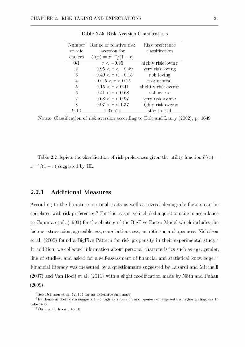
Table 2.2: Risk Aversion Classifications
Number Range of relative risk Risk preferenceof safe aversion for classificationchoices U(x) = x1−r/(1− r)
0-1 r < −0.95 highly risk loving2 −0.95 < r < −0.49 very risk loving3 −0.49 < r < −0.15 risk loving4 −0.15 < r < 0.15 risk neutral5 0.15 < r < 0.41 slightly risk averse6 0.41 < r < 0.68 risk averse7 0.68 < r < 0.97 very risk averse8 0.97 < r < 1.37 highly risk averse
9-10 1.37 < r stay in bed
Notes: Classification of risk aversion according to Holt and Laury (2002), p: 1649
Table 2.2 depicts the classification of risk preferences given the utility function U(x) =
x1−r/(1− r) suggested by HL.
2.2.1 Additional Measures
According to the literature personal traits as well as several demografic factors can be
correlated with risk preferences.8 For this reason we included a questionnaire in accordance
to Caprara et al. (1993) for the eliciting of the BigFive Factor Model which includes the
factors extraversion, agreeableness, conscientiousness, neuroticism, and openness. Nicholson
et al. (2005) found a BigFive Pattern for risk propensity in their experimental study.9
In addition, we collected information about personal characteristics such as age, gender,
line of studies, and asked for a self-assessment of financial and statistical knowledge.10
Financial literacy was measured by a questionnaire suggested by Lusardi and Mitchelli
(2007) and Van Rooij et al. (2011) with a slight modification made by Noth and Puhan
(2009).
8See Dohmen et al. (2011) for an extensive summary.9Evidence in their data suggests that high extraversion and openess emerge with a higher willingness to
take risks.10On a scale from 0 to 10.

CHAPTER 2. RISK TAKING AND EXPECTATIONS 22
2.2.2 Execution
We used ORSEE Greiner (2004) to recruit 157 subjects (71 females, 83 males) from the
University of Hamburg without any restrictions. Individuals were aged between 19 and
37.11 The experiment was computerized via LIMESURVEY12 and took 30 minutes on
average to complete. 15 subjects, randomly selected, earned e 62.78 on average from all
tasks.
2.3 Theories and Predictions
According to the common working models for choices under risk, Harrison and Rutstrom
(2008) highlight that choices over lotteries are generally determined by one to three
parameters: the degree of risk aversion, the degree of loss aversion and the degree of
probability weighting. Therefore, models of decision under risk are only distinguished in
the focusing of one or more of these parameters. We discuss several well-established models
of decisions under risk in the following subsections. In the second part of Section 2.4, we
estimate these models via Maximum Likelihood Methods on our data in order to reveal
the mechanism and motivation behind expectation-induced risk taking.
The choice variable for every model we discuss is the stage in which subjects are
indifferent between choosing Lottery A or Lottery B. This stage is represented by the
probability p∗ on the first outcomes of Lottery A (2.0, 1.6, p) and Lottery B (3.85, 0.1, p).
Therefore, p is 1/10 for the first stage and 10/10 for the tenth stage. Thus, the higher the
value for p, the higher the stage in which a subject decides to switch from Lottery A to
Lottery B.
p∗1.6 + (1− p∗)2.0 ≤ p∗3.85 + (1− p∗)0.1 (2.1)
2.3.1 Expected Utility Theory
Our starting point is a risk-neutral Von-Neumann-Morgenstern rational decision maker
who would start by choosing Lottery A and switch to Lottery B in the fifth stage for
p∗ = 0.5.
11The 90 percent percentile was 28 years. We excluded all subjects > 30 years for our statistical analysis(see section results).
12www.limesurvey.com

CHAPTER 2. RISK TAKING AND EXPECTATIONS 23
p∗1.6 + (1− p∗)2.0 ≤ p∗3.85 + (1− p∗)0.1 (2.2)
p∗ ≤ 1.9
3.35< 0.6 (2.3)
If we include risk aversion via a utility function u(x) with constant relative risk aversion
(CRRA), the switching point is determined by the degree of risk aversion r.
u(x) =x1−r
1− r(2.4)
EUA(p∗) ≤ EUB(p∗) (2.5)
p∗(r) ≤ u(0.1)− u(1.6)
u(2)− u(3.85)− u(1.6) + u(0.1)(2.6)
Based upon the classification of Holt and Laury (2002) (Table 2.2), a risk-averse decision
maker would choose Lottery A five times or more. According to the independence axiom
Von Neumann and Morgenstern (1947), the fixed amount of 3.5 should have no influence
on his decision since it occurs with probability of 0.5 for both tasks: if A � B, then
123.5 + 1
2A � 1
23.5 + 1
2B. Thus, we convert the Allais-Paradoxon into a gradual form.
Within the EUT-framework, different risk taking behavior between both lottery tasks of
our setup (Holt Laury vs. modified Holt Laury) can only be explained with a change in the
degree of risk aversion (r). Since the fixed amount lies within the range of possible lottery
outcomes, EUT cannot provide an explanation for different choice-behavior independently
from the form of the utility function.
Prediction EUT: An EUT-maximizer would choose the same number of A-lotteries for
the standard and the modified HL-lotteries.
2.3.2 Expected Utility Alternatives
Alternatives to EUT number into double figures up to now (e.g., Starmer (2000), Fehr-Duda
and Epper (2012)). Thus, the question is how to select a tractable number of models for
our study. Fehr-Duda and Epper (2012) suggest deriving some working models for choices

CHAPTER 2. RISK TAKING AND EXPECTATIONS 24
under risk by three requirements: (1) basic properties such as completeness, transitivity,
continuity, and monotonicity; (2) first-order risk aversion; and (3) probability distortion.
The latter requirements are due to empirical validity. Thereby, the authors distill two
main models: (1) rank-dependence models (e.g., Quiggin (1982), Tversky and Kahneman
(1992)) and (2) disappointment aversion (Gul (1991)). We also take into account Salience
Theory (ST) Bordalo et al. (2012), since this theory combines rank-dependence and a kind
of disappointment aversion.
Rank Dependence Models
According to Fehr-Duda and Epper (2012), rank-dependence models can be divided into
Cumulative Prospect Theory (CPT) (Tversky and Kahneman (1992)) and rank dependent
utility (RDU) (Quiggin (1982)).
Cumulative Prospect Theory
Based on the assumption that the fixed amount works as a reference point, the loss in the
sense of Kahneman and Tversky (1979) a decision maker perceives does not affect risk
taking behavior, which she would reveal for the (standard) HL-lotteries.
(2.7)
U(xi) = EV (xi) +
EV (xi)− rp; EV (xi)− r > 0
λ(EV (xi)− rp); else, i = A,B
For any loss aversion parameter λ ≥ 0.4813, Option B provides a bigger loss (LB)
LBj = (1−p)(3.85−3.5)+pλ(0.1−3.5) ≥ LAj = (1−p)λ(2−3.5)+pλ(1.6−3.5)14 (2.8)
than the loss a subject perceives from Option A (LA) in the first four stages. Thus, a
loss-averse decision maker would switch from Option A to Option B in the fifth stage or
later.
CPT has the same implications as the rank dependence model utility (RDU) of Quiggin
(1982) for the case that loss aversion is of no relevance. The second driver for choice
13A loss aversion parameter ≤ 1 implies loss seeking behavior.14A decision maker who follows (origin) Prospect Theory would not take the fixed amount into account
(as part of a compounded lottery) since common consequences are assumened to be canceled out in theediting phase.

CHAPTER 2. RISK TAKING AND EXPECTATIONS 25
behavior in the CPT framework is rank-dependent probability weighting as suggested by
Quiggin (1982). Thus, the CPT model has the same implications as the RDU-model we
will focus on in the following.
Rank Dependent Utility
The intuition behind RDU in the sense of Quiggin (1982) is that possible outcomes of
a lottery are firstly ranked by the level of aspiration.1516 Afterwards, the probabilities
are replaced through decision weights, which are defined as in Equation 2.11. There
are two differences to standard probability weighting: (1) small probabilities are only
overweighted if a low rank is attached to the corresponding outcome, (2) a violation of
first-order stochastic dominance cannot occur, since decision weights are derived from the
entire distribution of probabilities.17
V (P ) =n∑i=1
πiu(xi) (2.9)
πi =
w(p1) for i = 1
w(i∑
k=1
pk)− w(i−1∑k=1
pk) for 2 ≤ i ≤ n(2.10)
There are numerous specifications of the probability weighting function (Harrison and
Rutstrom (2008) for a detailed discussion). We chose the weighting function suggested by
Karmarkar (1979) since this functional form ensures that there is no interdependence of the
weighting parameter γ and the degree of risk aversion r. By doing this, we can differentiate
between a shift in probability distortion and a variation in the degree of risk aversion.
w(p) =pγ
pγ + (1− p)γ(2.11)
15In this context, the salience of an outcome is often synonymically used. As we will discuss, there is adifference between salience in the sense of Bordalo et al. (2012) and salience in the meaning of: outstanding,unique, etc.
16Koszegi and Rabin (2006) revisit RDU and extend this model with a so called personal equilibrium.17This is the main innovation of Cumulative Prospect Therory (Tversky and Kahneman (1992)) in
comparison to Prospect Theory (Kahneman and Tversky (1979)).

CHAPTER 2. RISK TAKING AND EXPECTATIONS 26
Disappointment Aversion
The basic idea of disappointment aversion (DA) (Bell (1985), Loomes and Sugden (1986)
and Gul (1991)) is that a DA-maximizer perceives the potential outcomes of a lottery
as either disappointing or aspired. Thus, all outcomes are evaluated in relation to a
disappointment-threshold. Fehr-Duda and Epper (2012) show that DA-theory is a special
of rank dependent theory with only two ranks for (1) aspired outcomes, and (2) disappointing
outcomes. There are different notions of disappointment aversion (i.e., Grant et al. (2001)
and Routledge and Zin (2010) for an overview). The main difference is the definition of the
disappointment-threshold. Whereas Bell (1985) suggests the expected value as a candidate,
Gul (1991) applies the certainty equivalent (CA). We employ the model of Grant and
Kajii (1998). The authors suggest that disappointment/elation is perceived in relation to
the best outcome of a lottery. Since we want to investigate the effect of achievable but
unrealistic outcomes, we use this notion for further analyses.
V (P ) =
∫x
u(x)d[FP (x)γ] (2.12)
FP is a cumulative distribution function as in Equation 2.9. The additional utility of
outcome xi which occurs with probability pi to the overall utility V (P ) of a lottery is
v(pi) = [(pi + qi)γ − qγi ]u(xi), (2.13)
where qi is the probability that the lottery yields an outcome worse than xi. As can be
easily shown, a subject is disappoint-averse if (and only if) γ < 1. For the case γ = 1, the
DA-model converts to EUT.
Salience Theory
Bordalo et al. (2012) suggest a model (ST - Salience Theory) for decisions under risk which
is driven by the idea that probabilities are more distorted the more salient an outcome
is. So far, this is common to the rank dependence models we discussed before. The main
difference lies in the definition of a context-dependent salience (σ) for all possible outcomes
xi
σ(xiS, x−iS ) =
| xiS − x−iS || xiS | + | x
−iS |
(2.14)

CHAPTER 2. RISK TAKING AND EXPECTATIONS 27
S is the state (context) for which an outcome is assessed. Applied to the standard
HL-lotteries, a decision maker following ST would identify four states:
S1(1.6, 3.85), S2(1.6, 0.1), S3(2.0, 3.85), S4(2.0, 0.1).
The modified HL-lotteries provide eight states, due to the comparison of every lottery
outcome with the fixed amount:
S1(1.6, 3.85), S2(1.6, 0.1), S3(2.0, 3.85), S4(2.0, 0.1)
S5(3.5, 3.85), S6(3.5, 0.1), S7(3.5, 1.6), S8(3.5, 2.0).
For our design, this means that each possible outcome of Lottery A is valued in the
context of every possible outcome of Lottery B and vice versa. Bordalo et al. (2012)
highlight the fact that contrary to origin PT, outcomes are not over- or underweighted if
they are high or low. These outcomes are only overweighted if they are salient. ST would
predict a decrease in risk taking. This effect is due to the fact that S6 is the most salient
state and subjects become more aware of the risk of Option B.
2.4 Results
According to Holt and Laury (2002), we define the A-lotteries for both main tasks as safe
choices in contrast to the high variance B-lotteries. Thus, risk taking is defined as switching
from Lottery A to Lottery B. We use the difference of chosen A-lotteries between both
tasks as measure for expectation-induced risk taking.
2.4.1 Descriptive Results
As a first step, we only pay attention to subjects who only switched once, from Option A
to Option B. Thus, we exclude 23 subjects (a portion of 14.6 percent) from the further
analysis since they switched back from Option B to Option A (multiple switchers).18 As
shown in Figure 2.1, risk taking is higher for the modified HL-lotteries (MHL) than for
the HL-lotteries. The straight dash-dot-line represents an expected value maximizer (risk
18This phenomena is common for Multiple Price Lists. HL report a portion of 13.2 percent of multipleswitchers.

CHAPTER 2. RISK TAKING AND EXPECTATIONS 28
neutrality). The cumulative proportion of chosen A-lotteries for the MHL-lotteries is
greater than for the HL-lotteries for every number of safe choices. This difference in risk
taking is significant using a Wilcoxon-signed-rank test of the null hypothesis that there is
no intra-subject difference in the number of chosen safe choices between the standard and
the modified HL-lotteries (p < 0.01).19
Result: On average, subjects played one less A-lottery in the modified than in the
standard HL-lotteries.
Figure 2.1: Cumulated Fraction of Safe Choices — HL + MHLall subjects
0.2
.4.6
.81
Frac
tion
of S
afe
Cho
ices
0 1 2 3 4 5 6 7 8 9 10Decision
Induced Expectations No Induced Expectations
Notes: This figure illustrates the cumulative fraction of safe choices (A) for all subjectsover all stages (1 - 10) for the HL and MHL-task. The third graph (straight line) representsa rational risk neutral decision-maker.
More than fifty percent of 134 subjects increased their risk taking by switching from
Option A to Option B in the modified HL-lotteries, as compared to the standard HL-
lotteries by at least one stage earlier. 53 subjects (40 percent) did not change their behavior
and 13 subjects decreased their risk taking by switching to Option B in a later stage. Based
on these results, we identify two types of decision makers: susceptible and non-susceptible
for induced reference points.20
19We excluded multiple switchers from our main analysis as suggested by Holt and Laury (2002).20The third group of 13 subjects who decreased their risk taking by switching to Option B later in the
modified HL-lotteries is statistically too small for further analysis.

CHAPTER 2. RISK TAKING AND EXPECTATIONS 29
Figure 2.1 illustrates that on average, subjects switched in the fifth stage from the
safe option to the risky one in the standard HL MPL. According to the risk aversion
classification of Table 2.2, these subjects are slightly risk averse on average. The average
switching point for the modified MPL is the fourth stage. According to Table 2.2, the same
subjects reveal risk neutrality. The following example is designed to provide an intuition of
this effect: a risk-neutral decision maker would be indifferent between a fixed amount (i.e.,
certainty equivalent) of 100, 000 and a lottery of 0.5; 50, 000 and 0.5; 150, 000. In accordance
with Holt and Laury (2002), we use the following utility function: U(x) = x1−r/(1− r) to
calculate the certainty equivalent and a risk aversion parameter of 0.28 as seen in Table 2.2.
A slightly risk averse person would choose the lottery if the fixed amount was nearly 90, 000.
Figure 2.2: Cumulated Fraction of Safe Choices — HL+ MHLRP-Susceptives
0.2
.4.6
.81
Frac
tion
of S
afe
Cho
ices
0 1 2 3 4 5 6 7 8 9 10Decision
Induced Expecatations No Induced Expectations
Notes: This figure illustrates the cumulative fraction of safe choices (Lottery A) for theRP-susceptive subjects over all stages (1 - 10) for the HL and MHL-task. The third graphrepresents a rational risk-neutral decision maker.
Next, we explore the mechanism behind expectation-induced risk taking. The focus on
the group of subjects with an increased willingness to take risks (RP-susceptives) reveals
that, on average, this group is risk-averse if playing the HL-lotteries and risk-neutral for
the modified HL-lotteries as shown in Figure 2.2. Table 2.3 and Table 2.4 itemize the
choice behavior of both main groups. NON-RP-susceptives are slightly risk averse for both
tasks (median).

CHAPTER 2. RISK TAKING AND EXPECTATIONS 30
Table 2.3: Descriptive Results — RP-Susceptives
Task N Mean SD Min 0.25 Quant. Median 0.75 Quant. MaxHolt & Laury 68 5.71 1.75 2.00 5.00 6.00 7.00 10.00Holt & Laury RP 68 3.60 1.84 0.00 3.00 4.00 5.00 8.00
Notes: 68 subjects, who chose less safe lotteries in the first task in contrast to the secondtask, were risk averse for the standard HL-lotteries und slightly risk loving for the modifiedlottery task.
Table 2.4: Descriptive Results — NON-RP-Susceptives
Task N Mean SD Min 0.25 Quant. Median 0.75 Quant. MaxBoth Tasks 53 4.64 1.43 0.00 4.00 4.00 5.00 10.00
Notes: 53 subjects who chose the same amount of safe lotteries for both main tasks, wererisk neutral on average.
As can be seen in Figure 2.2 and Table 2.3, RP-susceptives increased their risk taking
by switching nearly two stages later from the safe choice A to the high-variance lottery B.
The main descriptive result is that RP-susceptives are risk-averse for the HL-lotteries
(Table 2.3: 5.71 safe choices on average), whereas NON-RP-susceptives tended to be
risk-neutral for this task (Table 2.4: 4.64 safe choices on average).
The results of an ordered probit regression on the difference of chosen A-lotteries
between both main tasks are presented in Section A.1.1 of the Appendix.
2.4.2 Model Estimation and Selection - Specifying the Reference
Point
Abeler et al. (2011) highlight the fact that specifying the reference point of expectation-
based models is an important direction for future research. One can argue that as long
as there is no empirical supported reference point model, econometrical estimations will
always be inherent to an additional degree of freedom.
So far, there are two main classes of models with different specifications of the reference
point: the first class, disappointment aversion, assumes that the reference point is some
level of aspiration (see Gul (1991) or Grant et al. (2001)). All possible outcomes of a lottery
are evaluated in contrast to one desired outcome (i.e., the highest possible outcome, as

CHAPTER 2. RISK TAKING AND EXPECTATIONS 31
suggested by Grant et al. (2001)). In the second class, the reference point is the whole
distribution of the ranks of possible outcomes (see Quiggin (1982) or Koszegi and Rabin
(2006) and Koszegi and Rabin (2007)). According to our experiment design, the fixed
amount introduced in the second task should have two different functions, depending on
the choice model: in DA, it directs attention to the highest possible outcome, which is
3.85 of the risky choice (Option B). In RDU, it changes the distribution of the ranks of
possible outcomes. In order to understand the meachnism behind RP-induced risk taking,
we estimate the parameters of our working models discussed in Section 3 via Maximum
Likelihood Methods as suggested by Harrison et al. (2007). The utility (Ui), where i = A,B,
for both Lotteries A and B, is defined as in Equations 2.9 and refe12The difference (∇) for
every lottery pair A and B is
∇U = UA − UB (2.15)
per stage. Thus, a subject will choose Lottery A if ∇U > 0.
We assume that subjects make some errors when comparing Lottery A and Lottery B,
for example, in calculating expected values. Therefore, we add the Luce error specification
(µ) suggested by Luce and Fishburn (1991) to our estimations, which is also suggested by
Holt and Laury (2002).21
∇Uµ =U
1/µB
U1/µA + U
1/µB
(2.16)
Thus, the log-likelihood-function for the assumption that the EUT-model is true is
lnLEUT (r, µ, y) =∑i=1
[(ln((∇Uµ/µ) | yi = 1) + (ln(1− Φ(∇U/µ) | yi = 0)], (2.17)
with Φ() for the standard normal cumulative distribution function and yi with i = 0, 1
as an indicator-variable for individual choices (yi = 1 for the selection of Option A). If we
assume that the rank-dependence-models (RD and DA) are true, we have to estimate the
rank parameter (γ) in addition. The log-likelihood-function for the RD and DA-models
21See Harrison and Rutstrom (2008) for a survey of the advantages and disadvantages of several errorspecifications. The measure suggested by Luce and Fishburn (1991) has the advantage that ∇Uµ is alreadynormalized for its application in the log-likelihood-function.

CHAPTER 2. RISK TAKING AND EXPECTATIONS 32
equals:
lnLRD,DA(r, γ, µ, y) =∑i=1
[(ln(Φ(∇Uµ/µ) | yi = 1) + (ln(1− Φ(∇Uµ/µ) | yi = 0)]. (2.18)
Expected Utility Theory (EUT) - Maximum Likelihood Estima-
tion (MLE)
We start the MLE with the EUT-benchmark. It is obvious that the revealed difference in
risk taking behavior must be captured by the degree of risk aversion r, the noise parameter
µ, or both. The Maximum Likelihood estimates (Table 2.5) show that the estimates for
the risk aversion parameter (r) are in the range for risk neutrality (−0.15 < r < 0.15) and
slight risk aversion (0.15 < r < 0.41) (see Table 2.2). The most important result for the
estimation of the EUT-model is that the noise parameter (µ) cannot explain induced risk
taking for the modified HL-lotteries, since a decrease in the risk aversion parameter r (and
a decrease in the noise parameter) captures this behavior. Thus, we have evidence that
the increased willingness to take risks for the modified MPL is not due to confusion.
Table 2.5: Maximum Likelihood Estimates: Expected Utility (CRRA)
Parameter Variable Estimation Std. Error p-Value log-likelihood
HL-lotteries -386.6459r Constant 0.2808 0.0186 0.0000µ Constant 0.1269 0.0063 0.0000
MHL-lotteries -470.5786r Constant -0.0059 0.0019 0.0000µ Constant 0.0229 0.0248 0.0000
Weber et al. (2012) show that mere risk preferences (here r) are quite stable. Thus,
following our hypothesis that expectations can determine the reference point and thereby
also have a bearing on risk preferences, we estimate two reference point specifications
(RDU and DA) as discussed before and perform a horse race between these two models.

CHAPTER 2. RISK TAKING AND EXPECTATIONS 33
Rank Dependent Utility (RDU) - Maximum Likelihood Estima-
tion
According to the RDU-model (Equations 2.9-2.12) the focus of our RDU-estimation is
on the weighting parameter γ. If γ was equal to 1, the RDU-model would have the same
structure (i.e., consequences) as EUT. Equations 2.11 and 2.12 imply that the degree of
rank dependence increases with a decreasing γ.
As one can see in Table 2.6, in the case of the standard HL-lotteries, the estimator for γ is
close to 1 and has a standard error of (0.3547). The Wald-test on the hypothesis H0 : γ = 1
(1.1783) shows that χ2(1) = 0.25, p = 0.6152.
Thus, we cannot reject the hypothesis that subjects follow EUT in the HL-task. The
main result of our RDU-estimations is that for the case of the modified HL-lotteries,
the hypothesis that subjects do not distort probabilities and rank possible outcomes
cannot be rejected. The estimation of the distortion-parameter γ = 0.7548 is not equal
to 1. A chi-squared-test on this hypothesis (H0 : γ = 1) confirms the assumption
χ2(1) = 13.72, p = 0.0002. Hence, there is evidence that the induced reference point
can affect the attractiveness of lottery outcomes and that our subjects ranked possible
lottery-outcomes in relation to the fixed amount.

CHAPTER 2. RISK TAKING AND EXPECTATIONS 34
Table 2.6: Maximum Likelihood Estimates: Rank Dependence (Quiggin 1982)
Parameter Variable Estimation Std. Error p-Value log-likelihood
HL-lotteries -386.06697r Constant 0.2921 0.04286 0.0000γ Constant 1.1783 0.3547 0.0010µ Constant 0.1396 0.0242 0.0000
MHL-lotteries -458.4372r Constant -0.1679 0.0744 0.0240γ Constant 0.7548 0.0662 0.0000µ Constant 0.0631 0.0085 0.0000
Disappointment Aversion (DA) - Maximum Likelihood Estima-
tion
The reference point of a DA decision maker is not determined by the whole distribution as
in RDU-theory. Fehr-Duda and Epper (2012) highlight the fact that DA means that there
are only two ranks: above and below the reference point. According to Equation 2.14, a
decision maker is disappointment averse if (and only if) γ < 1. For the case of γ = 1, the
DA-model converts to EUT. In reference to our experiment design, we assume that the
highest outcome, which is 3.85 of the risky choice (Option B), works as reference point. So,
the fixed amount (3.5) has directed the subject’s attention to this outcome.
Table 2.7 shows the results for both main tasks. If we test (Wald-test) the H0 : γ = 1
for the modified lotteries, the result ist χ2(1) = 126.87, p = 0.0000; whereas we cannot
reject this hypothesis for the standard HL-lotteries, as χ2(1) = 2.38, p = 0.1225. Our
ML-estimations provide evidence that the fixed amount could have directed attention to
the highest lottery outcome and could have induced a higher willingness to take risks due
to disappointment aversion.
Model Selection
In this section, we try to provide evidence for the question how the reference point
is specified. According to our model estimations, we have two candidates: the whole

CHAPTER 2. RISK TAKING AND EXPECTATIONS 35
Table 2.7: Maximum Likelihood Estimates: Disappointment Aversion
Parameter Variable Estimation Std. Error p-Value log-likelihood
HL-lotteries -384.9142r Constant 0.3117 0.0155 0.0000γ Constant 1.9078 0.5878 0.0010µ Constant 0.1147 0.0239 0.0000
MHL-lotteries -443.5302r Constant 0.5943 0.0052 0.0000γ Constant 0.8122 0.0167 0.0000µ Constant 0.0720 0.0043 0.0000
Table 2.8: Model Selection HL-lotteries
Model Degrees of AIC BIC Rank AIC Rank BICFreedom (k)
EUT 2 777.29 783.08 2 1RD 3 778.14 786.83 3 3DA 3 775.83 784.52 1 2
distribution (RDU) or an aspiration level (i.e., the highest outcome) as suggested in DA.
Thus, we start a horse race between our estimated working models.
One approach, given the log-likelihood of an estimated model, is the Akaike Information
Criterion (AIC) (Akaike (1973) and Akaike (1974)) where k stands for the number of
parameters (i.e., degrees of freedom).
AIC = −2ln(likelihood) + 2k (2.19)
Since we compare models with different amounts of parameters, we prefer the Bayesian
Information Criterion (BIC) because the BIC takes additional degrees of freedom more
into account than the AIC.
BIC = −2ln(likelihood) + ln(N)k (2.20)
Since N stands for the number of subjects, the penalty component for the BIC is more
influential than the component of the AIC for more than eight observations (N ≥ 8).
Table 2.8 and 2.9 content the results for both lottery-tasks. Given Equation 2.19
and 2.20 it is obvious that the smaller the AIC or BIC the more likely the model is (given
the range of models).

CHAPTER 2. RISK TAKING AND EXPECTATIONS 36
Table 2.9: Model Selection MHL-lotteries
Model Degrees of AIC BIC Rank AIC Rank BICFreedom (k)
EUT 2 945.16 950.95 3 3RD 3 922.87 931.57 2 2DA 3 893.06 901.75 1 1
The most important result is that in the first task (modified HL-lotteries) the DA model
has the lowest BIC while in the second task (standard HL-lotteries), it is the EUT-model
with the lowest BIC. Given our set of models, these results provide evidence for:
1. EUT is still a reliable model to explain risk preferences for less complex choices.22
2. In a more complex decision task (MHL) with the chance of a high outcome (i.e., fixed
amount), subjects define some level of aspiration.
2.4.3 Robustness Checks
Randomness
There is an intuitive assumption that the modified HL-lottieries provoke a more random
choice behavior. We want to highlight the fact that for the Maximum Likelihood estimations
of all three working models, we find a decrease (from the standard HL-lotteries in contrast
to the modified lotteries) in the estimations of the noise parameter (µ).23 This finding is
in line with the hypothesis that reference points can simplify decision tasks by drawing
attention to one aspect (outcome) of a complex decision task (e.g., Brandstatter et al.
(2006)).
Compatibility and Ordering
According to the Rabin-Critique (Rabin (2000)), one might argue that the small stakes
of our lotteries were not incentive compatible. Therefore, we implemented a control task
which all subjects had to play after the two main tasks. This task was similar to the
first task (modified HL-lotteries) with the only modification being that subjects received
as payoff the result of ten draws with replacement of their chosen lotteries at the end
22This hypothesis might be supported by the fact that multiple price lists (e.g., HL) are frequently usedfor economic experiments and our subjects may have had some kind of experience.
23µ = 0 implies that there is no evidence for structural errors made by our subjects (i.e., errors incalculating expected values)

CHAPTER 2. RISK TAKING AND EXPECTATIONS 37
Figure 2.3: Control Task — HL-lotteries with 10 Draws
0.2
.4.6
.81
Frac
tion
of S
afe
Cho
ices
0 1 2 3 4 5 6 7 8 9 10Decision
No Induced ExpectationsInduced Expectations (10 Draws)
of the experiment. We also used this task to control for an ordering effect. All subjects
passed through the experiment in the following sequence: modified HL-lotteries (1 draw),
standard HL-lotteries (1 draw), modified HL-lotteries (10 draws). If there was an ordering
or learning effect, the results of the third (control) task would have significantly differed
from the first task.
Our findings show that individual willingness to take risk for the control task rises
significantly in contrast to the previous task (mere HL-lotteries). This difference in risk
taking is significant using a Wilcoxon-signed-rank test of the null hypothesis that there
is no intra-subject difference in the number of chosen safe choices between the standard
HL-lotteries and the control task (p < 0.01). Thus, on average, subjects increased their
risk taking for the first and third task in contrast to the mere HL-lotteries, the second task.
Result 1b: On average, subjects played 1 less A-lotteries in the modified than in the
standard HL-lotteries. Thus, subjects are willing to take more risk if they can expect to
earn an amount that is beyond their (mere) risk preference.
MPL and Multiple Switchers
We excluded 22 subjects for switching twice or more between A- and B-lotteries for our basic
analyses. Our results stay robust if we reinclude these subjects for a Wilcoxon-signed-rank

CHAPTER 2. RISK TAKING AND EXPECTATIONS 38
test of the null hypothesis that there is no intra-subject difference in the number of played
A-lotteries between the standard and the modified HL-lotteries.
2.5 Conclusion
We provide evidence that expectations can induce a reference point and risk taking.
Subsequently, we localize the specifications of the reference point. Within a compensation
framework we show that, given a relatively high salary, the highest possible outcome of a
risky choice is a reasonable candidate for the reference point.
According to Gothmann (2015), who suggests that a cap on bonus payments can
have external effects (e.g., increased risk taking), we can localize potential mechanisms of
such a behavior. An important question for future research is whether our findings have
implications for financial markets (i.e., asset prices).
Recent initiatives of European regulatory authorities are focused on compensation
schemes (e.g., bonus cap) of credit and investment banks. With regard to our findings,
one must ask whether such interventions take aspects as, for instance, reference dependent
preferences and their impact on individual risk preferences into account.

CHAPTER 2. RISK TAKING AND EXPECTATIONS 39
References
Abeler, Johannes, Armin Falk, Lorenz Goette, and David Huffman (2011). “Reference
Points and Effort Provision”. American Economic Review, 470–492.
Akaike, Hirotugu (1973). “Information Theory and an Extension of the Maximum Likelihood
Principle”. In: Second International Symposium on Information Theory. Akademinai
Kiado, 267–281.
Akaike, Hirotugu (1974). “A New Look at the Statistical Model Identification”. Automatic
Control, IEEE Transactions on 19(6), 716–723.
Bebchuk, Lucian A and Jesse M Fried (2009). Pay Without Performance: The Unfulfilled
Promise of Executive Compensation. Harvard University Press.
Bell, David E (1985). “Disappointment in Decision Making under Uncertainty”. Operations
Research, 1–27.
Bernoulli, Daniel (1738). “Theoremata de Oscillationibus Corporum Filo Flexili Con-
nexorum et Catenae Verticaliter Suspensae”. Comm. Acad. Sci. Petrop 6(1732-1733),
108–122.
Bordalo, Pedro, Nicola Gennaioli, and Andrei Shleifer (2012). “Salience Theory of Choice
Under Risk”. Quarterly Journal of Economics 127(3), 1243–1285.
Brandstatter, Eduard, Gerd Gigerenzer, and Ralph Hertwig (2006). “The Priority Heuristic:
Making Choices Without Trade-Offs”. Psychological Review 113(2).
Camerer, Colin, Linda Babcock, George Loewenstein, and Richard Thaler (1997). “Labor
Supply of New York City Cabdrivers: One Day at a Time”. Quarterly Journal of
Economics 112(2), 407–441.
Caprara, Gian Vittorio, Claudio Barbaranelli, Laura Borgogni, and Marco Perugini (1993).
“The ’Big Five Questionnaire’: A New Questionnaire to Assess the Five Factor Model”.
Personality and Individual Differences 15(3), 281–288.
Cialdini, Robert, Melanie Trost, and Jason Newsom (1995). “Preference for Consistency:
The Development of a Valid Measure and the Discovery of Surprising Behavioral
Implications.” Journal of Personality and Social Psychology 69(2), 318.

CHAPTER 2. RISK TAKING AND EXPECTATIONS 40
Crawford, Vincent P and Juanjuan Meng (2011). “New york city cab drivers’ labor supply
revisited: Reference-dependent preferences with rationalexpectations targets for hours
and income”. The American Economic Review 101(5), 1912–1932.
Dohmen, Thomas, Armin Falk, David Huffman, Uwe Sunde, Jurgen Schupp, and Gert G
Wagner (2011). “Individual Risk Attitudes: Measurement, Determinants, and Behavioral
Consequences”. Journal of the European Economic Association 9(3), 522–550.
Fahlenbrach, Rudiger, Robert Prilmeier, and Rene M Stulz (2012). “This Time Is the
Same: Using Bank Performance in 1998 to Explain Bank Performance During the Recent
Financial Crisis”. Journal of Finance 67(6), 2139–2185.
Fahlenbrach, Rudiger and Rene M Stulz (2011). “Bank CEO Incentives and the Credit
Crisis”. Journal of Financial Economics 99(1), 11–26.
Falk, Armin and Florian Zimmermann (2011). “Preferences for Consistency”. Working
Paper.
Fehr-Duda, Helga and Thomas Epper (2012). “Probability and Risk: Foundations and
Economic Implications of Probability-Dependent Risk Preferences”. Annu. Rev. Econ.
4(1), 567–593.
Frederick, Shane and George Loewenstein (1999). “Hedonic Adaptation”.
Gothmann, Roger (2015). “Risk Taking and Compensation Schemes”. Working Paper.
Grant, Simon and Atsushi Kajii (1998). “AUSI Expected Utility: An Anticipated Util-
ity Theory of Relative Disappointment Aversion”. Journal of Economic Behavior &
Organization 37(3), 277–290.
Grant, Simon, Atsushi Kajii, and Ben Polak (2001). “Different Notions of Disappointment
Aversion”. Economics Letters 70(2), 203–208.
Greiner, Ben (2004). “An Online Recruitment System for Economic Experiments”. Forschung
und wissenschaftliches Rechnen 63, 79–93.
Gul, Faruk (1991). “A Theory of Disappointment Aversion”. Econometrica, 667–686.
Harrison, Glenn W, John A List, and Charles Towe (2007). “Naturally Occurring Preferences
and Exogenous Laboratory Experiments: A Case Study of Risk Aversion”. Econometrica
75(2), 433–458.

CHAPTER 2. RISK TAKING AND EXPECTATIONS 41
Harrison, Glenn W and Elisabet E Rutstrom (2008). “Risk Aversion in the Laboratory”.
Research in Experimental Economics 12, 41–196.
Holt, Charles A and Susan K Laury (2002). “Risk Aversion and Incentive Effects”. American
Economic Review 92(5), 1644–1655.
Huck, Steffen and Georg Weizsacker (1999). “Risk, Complexity, and Deviations from
Expected-Value Maximization: Results of a Lottery Choice Experiment”. Journal of
Economic Psychology 20(6), 699–715.
Kahneman, Daniel and Amos Tversky (1979). “Prospect Theory: An Analysis of Decision
under Risk”. Econometrica, 263–291.
Karmarkar, Uday S (1979). “Subjectively weighted utility and the Allais paradox”. Orga-
nizational Behavior and Human Performance 24(1), 67–72.
Koszegi, Botond and Matthew Rabin (2007). “Reference-Dependent Risk Attitudes”.
American Economic Review 97(4), 1047–1073.
Koszegi, Botond and Matthew Rabin (2006). “A Model of Reference-Dependent Prefer-
ences”. Quarterly Journal of Economics, 1133–1165.
Loomes, Graham and Robert Sugden (1986). “Disappointment and Dynamic Consistency
in Choice under Uncertainty”. Review of Economic Studies 53(2), 271–282.
Luce, R Duncan and Peter C Fishburn (1991). “Rank-And-Sign-Dependent Linear Utility
Models for Finite First-Order Gambles”. Journal of Risk and Uncertainty 4(1), 29–59.
Lusardi, Annamaria and Olivia Mitchelli (2007). “Financial Literacy and Retirement
Preparedness: Evidence and Implications for Financial Education”. Business Economics
42(1), 35–44.
Miller, Louis, David E Meyer, and John T Lanzetta (1969). “Choice Among Equal Expected
Value Alternatives: Sequential Effects of Winning Orobability Level on Risk Preferences.”
Journal of Experimental Psychology 79(3p1), 419.
Nicholson, Nigel, Emma Soane, Mark Fenton-O’Creevy, and Paul Willman (2005). “Per-
sonality and Domain-Specific Risk Taking”. Journal of Risk Research 8(2), 157–176.
Noth, Markus and Tatjana Puhan (2009). “How to Hide Mutual Fund Fees–Experimental
Evidence”. Working Paper.
CHAPTER 2. RISK TAKING AND EXPECTATIONS 42
Ockenfels, Axel, Dirk Sliwka, and Peter Werner (2014). “Bonus Payments and Reference
Point Violations”. Management Science 61(7), 1496–1513.
Quiggin, John (1982). “A Theory of Anticipated Utility”. Journal of Economic Behavior
& Organization 3(4), 323–343.
Rabin, Matthew (2000). “Risk Aversion and Expected-Utility Theory: A Calibration
Theorem”. Econometrica 68(5), 1281–1292.
Routledge, Bryan R and Stanley E Zin (2010). “Generalized Disappointment Aversion and
Asset Prices”. Journal of Finance 65(4), 1303–1332.
Starmer, Chris (2000). “Developments in Non-Expected Utility Theory: The Hunt for
a Descriptive Theory of Choice under Risk”. Journal of Economic Literature 38(2),
332–382.
Tversky, Amos and Daniel Kahneman (1992). “Advances in Prospect Theory: Cumulative
Representation of Uncertainty”. Journal of Risk and Uncertainty 5, 297–323.
Van Rooij, Maarten, Annamaria Lusardi, and Rob Alessie (2011). “Financial Literacy and
Stock Market Participation”. Journal of Financial Economics 101(2), 449–472.
Von Neumann, John and Oskar Morgenstern (1947). “The Theory of Games and Economic
Behavior”.
Weber, Martin, Elke U Weber, and Alen Nosic (2012). “Who Takes Risks When and Why:
Determinants of Changes in Investor Risk Taking”. Review of Finance 17, 847–883.

Chapter 3
Risk Taking and CompensationSchemes
43

CHAPTER 3. RISK TAKING AND COMPENSATION SCHEMES 44
3.1 Introduction
Aligning the interests of managers and owners of capital companies by means of monetary
incentives (i.e., remuneration) is one of the major challenges in management. Recent
insolvencies of (investment) banks and public subsidies for numerous financial institutions
during the last financial crisis have drawn public attention to the structure of executive
remuneration in the financial industry. Since financial institutions are highly leveraged
compared to conventional industry, individual decisions (i.e., risk taking) of their managers
have a considerable impact on economic welfare.
The objective of our study is to investigate the effect of recent regulatory measures in
the aftermath of the financial crisis, such as bonus caps, on individual decision making
(i.e., risk taking) by means of an experiment.
The influence of compensation schemes on excessive risk taking1 and misperceptions of
risk before the financial crisis must be separated from other aspects such as, for instance, a
supportive regulatory framework for subprime mortgage loans in the US and other effects.2
Nevertheless, there is some empirical evidence for a correlation of executive remuneration
practices and a biased perception of risk (e.g., Financial Stability Board (2009)). Bebchuk
and Fried (2009) analyze the pre-crisis compensation contracts of executives from several
investments banks. They find that bonus payments which were several times higher than
the fixed salary were connected to short-term gains, without, in most cases, any rules that
might allow banks to claw back bonus payments at least partially.
From an ex-post perspective it is obvious to conclude that such contracts can provide
incentives for investments in projects with short-term gains but a long-term negative net
present value.3 Fahlenbrach et al. (2012) analyze the performance and risk (i.e., leverage)
of banks during the financial crisis and find empirical evidence for this intuition. One effect
of these discussions is that compensation schemes have come in the focus of regulatory
authorities (Ferri and Goex (2013)).
The focus of our study is the impact of specific regulatory interventions in the aftermath
of the financial crisis on compensation schemes in the financial industry. One of the
1For the purposes of our study we use the definition suggested by Lefebvre and Vieider (2014). Theauthors define excessive risk taking as the choice of an inferior lottery (in comparison to a lottery with ahigher risk adjusted expected return).
2For instance Bouwman and Malmendier (2015) find evidence for an institutional memory of banks asdeterminant for risk taking.
3The concept ofMoral Hazard predicts such a behavior for cases when risks can be trasferred to debtholders or the government.

CHAPTER 3. RISK TAKING AND COMPENSATION SCHEMES 45
cornerstones of European financial market regulation was the publication of a directive in
2013.4 According to this directive, short-term bonus payment are capped to 100 percent of
yearly fixed compensation for executives of credit and investment banks.5 As a result a
wide range of financial institutions has raised the fixed salaries of their managers according
to a study of the EBA (2016).
Our research question is whether the relation of fixed and short-term variable bonus
payments can have an effect on risk taking. For this purpose we conduct an experiment.
Subjects have to choose between a high and a low variance lottery which is the same for
twenty stages. The only variable parameter for all stages is a fixed amount (i.e., fixed
salary) which is the same for every stage of Option A and Option B and which increases
by steps of one euro in order to study whether an increasing ratio of fixed versus variable
compensation has an influence on risk taking. A risk averse subject would choose the low
variance for every stage, whereas only a risk loving subject would prefer the high variance
lottery. According to neoclassical decision making theory a risk averse or risk loving subject
would never switch from Option A to Option B or vice versa. We can show that 10 percent
of our subjects start with choosing the high risk lottery in the first stage (i.e., low fixed
salary) whereas 54 percent have switched to the high variance lottery in the last stage (i.e.,
the highest fixed salary).
Our study is motivated by the works of Ockenfels et al. (2014) and Cole et al. (2015).
Both studies provide evidence that short-term bonus payments can have an effect on
individual decision making (i.e., risk taking). Since the authors of both studies conduct field
experiments we add additional value to this research question by investigating compensation
schemes by means of a controlled online experiment.
In Section 3.2 we provide an overview of the institutional framework for executive
compensation in the European Union (EU). Furthermore, we discuss current evidence on
remuneration practices in recent years. An overview of relevant literature is provided in
Section 3.3.
We discuss the theoretical framework of our analysis in Section 3.4 and explain the
design of our online experiment in Section 3.5. A discussion of our results is provided in
Section 3.6 and we complete our study with a conclusion in Section 3.7.
4Directive 2013/36/EU5Higher caps up to 200 percent (upper bound) have to be authorized by the general meeting.

CHAPTER 3. RISK TAKING AND COMPENSATION SCHEMES 46
3.2 Institutional Overview
In this section, we discuss the legal foundations for executive compensation of financial
institutions in the EU, which has received pronounced attention from the regulatory
authorities since the beginning of the financial crisis.
Adding to that, we provide a summary of empirical remuneration practices of European
financial institutions and discuss our findings in connection with the legal framework.
3.2.1 Legal Framework
A first comprehensive guideline for a reform and regulation of compensation schemes for
credit banks was published in 2009 by the Financial Stability Board (2009).
The European Commission incorporated these ideas into Directive 2010/76/EU, which
came into force on 1 January 2011. This directive provides, among other things, detailed
guidelines for the remuneration policies of credit institutions and investment firms (here:
financial institutions).
The Commission supplemented this regulatory frame by two additional directives in
2013 (2013/36/EU) (CRD IV) and 2014 (2014/604/EU). All three directives together were
introduced in the belief that remuneration practices were considered to have been among
the reasons that led decision makers of financial institutions to take excessive (short-term)
risks which resulted in the financial crisis, according to a study of the European Banking
Authority (EBA) (European Banking Authority (2014)).
We discuss two key measures of the legal framework described above. The first one is
defined in article 92 (2) of CRD IV which requires financial institutions to identify staff
(identified staff) who have, due to their professional activities, a material impact on the
institution’s risk exposure.
The identification criteria are a combination of quantitative and qualitative parameters.
According to the Directive 2013/36/EU, article 94 (2) identified staff are generally part of
the management body and/or have key functions or responsibilities over other identified
staff. The quantitative criteria are mainly based on remuneration: earnings of more than
500,000 euros per year or 0.3 percent of staff with the highest remuneration.
The EBA will provide specific guidelines on remuneration policies for identified staff.6
6The authority of the EBA to issue guidelines for remuneration policies in the financial industry of theEU is defined in articles 74 and 75 of Directive 2013/36/EU.
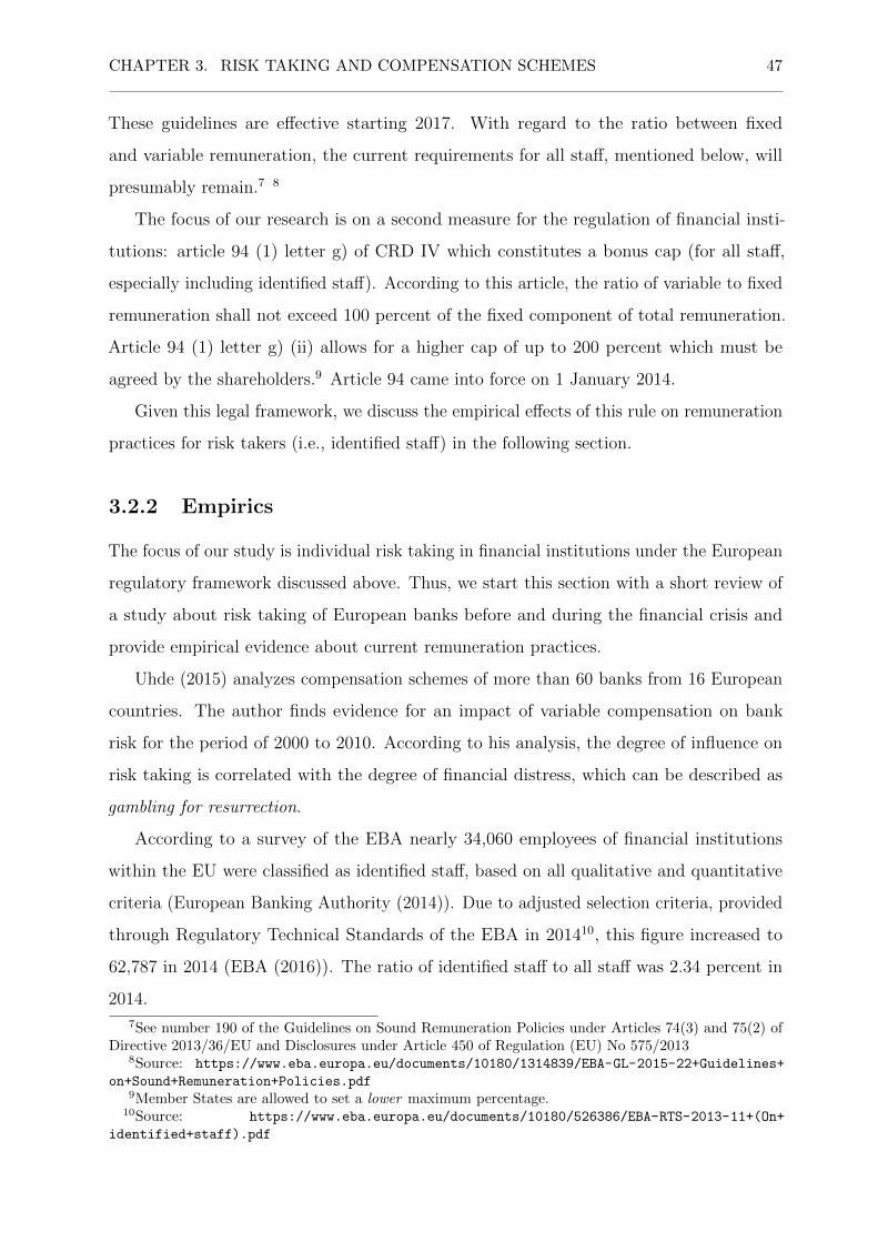
CHAPTER 3. RISK TAKING AND COMPENSATION SCHEMES 47
These guidelines are effective starting 2017. With regard to the ratio between fixed
and variable remuneration, the current requirements for all staff, mentioned below, will
presumably remain.7 8
The focus of our research is on a second measure for the regulation of financial insti-
tutions: article 94 (1) letter g) of CRD IV which constitutes a bonus cap (for all staff,
especially including identified staff). According to this article, the ratio of variable to fixed
remuneration shall not exceed 100 percent of the fixed component of total remuneration.
Article 94 (1) letter g) (ii) allows for a higher cap of up to 200 percent which must be
agreed by the shareholders.9 Article 94 came into force on 1 January 2014.
Given this legal framework, we discuss the empirical effects of this rule on remuneration
practices for risk takers (i.e., identified staff) in the following section.
3.2.2 Empirics
The focus of our study is individual risk taking in financial institutions under the European
regulatory framework discussed above. Thus, we start this section with a short review of
a study about risk taking of European banks before and during the financial crisis and
provide empirical evidence about current remuneration practices.
Uhde (2015) analyzes compensation schemes of more than 60 banks from 16 European
countries. The author finds evidence for an impact of variable compensation on bank
risk for the period of 2000 to 2010. According to his analysis, the degree of influence on
risk taking is correlated with the degree of financial distress, which can be described as
gambling for resurrection.
According to a survey of the EBA nearly 34,060 employees of financial institutions
within the EU were classified as identified staff, based on all qualitative and quantitative
criteria (European Banking Authority (2014)). Due to adjusted selection criteria, provided
through Regulatory Technical Standards of the EBA in 201410, this figure increased to
62,787 in 2014 (EBA (2016)). The ratio of identified staff to all staff was 2.34 percent in
2014.
7See number 190 of the Guidelines on Sound Remuneration Policies under Articles 74(3) and 75(2) ofDirective 2013/36/EU and Disclosures under Article 450 of Regulation (EU) No 575/2013
8Source: https://www.eba.europa.eu/documents/10180/1314839/EBA-GL-2015-22+Guidelines+
on+Sound+Remuneration+Policies.pdf9Member States are allowed to set a lower maximum percentage.
10Source: https://www.eba.europa.eu/documents/10180/526386/EBA-RTS-2013-11+(On+
identified+staff).pdf

CHAPTER 3. RISK TAKING AND COMPENSATION SCHEMES 48
The composition of the variable remuneration for identified staff mainly depends on
the business unit the employee works for. Figure 3.1 summarizes the distribution of
variable remuneration components according to the business units: investment banking,
retail banking, asset management, and other business areas for 2014. The focus of our
analysis, short-term cash linked instruments, make up between 50 and 70 percent of variable
compensation. These instruments are predominantly used in three of four bank units (EBA
(2016)).
Figure 3.1: Variable Remuneration for Identified Staff 2014
Investment Banking Retail Banking Asset Management Other Areas
Other InstrumentsShares/Share−LinkedCash
Components of Variable Remuneration
020
4060
8010
0
Notes: Data provided by EBA (2016)
The upper panel of Figure 3.2 shows a decrease in the ratio between variable and fixed
remuneration from 2010 to 2014 for identified staff. The variable pay for employees11 in
the asset management or the investment banking sector in 2014 is only one fourth of what
is was in 2010, which is due to the cap defined in Article 94 CRD IV. At the same time,
average fixed remuneration rose from 130,000 euros to 190,000 euros (panel 2 of Figure 3.2).
The EBA highlights that the rise of fixed salaries from 2010 to 2014 is characterized by
a high variance. In particular certain groups of identified staff could almost double their
fixed salary.
11In the following we use employee(s) as synonym for identified staff.

CHAPTER 3. RISK TAKING AND COMPENSATION SCHEMES 49
Figure 3.2: Variable Cash Component and Ratio of Fixed and Variable Remunerationfor Identified Staff (2010 - 2014)
2010 2011 2012 2013 2014
Investment BankingRetail BankingAsset ManagementOther Business Areas
Ratio of Variable & Fixed Remuneration for Identified Staff
050
100
150
200
250
300
350
2010 2011 2012 2013 2014
Average Fixed Remuneration for Identified Staff
050
000
1000
0015
0000
2000
00
Notes: Data aggregated from the EBA Reports ”Benchmarking of RemunerationPractices at Union Level, 2014 and 2016 (European Banking Authority (2014),EBA (2016))
Given the regulatory framework, we investigate the effect of this fundamental change of
structure of fixed and variable. There is evidence from the realm of behavioral economics
that this shift of compensation architecture might have an influence on the risk taking of
employees. The following section thus reviews the related literature.

CHAPTER 3. RISK TAKING AND COMPENSATION SCHEMES 50
3.3 Literature
There is a wide range of literature on the (optimal) structure of executive compensation.
Neoclassical models usually state that it is the fundamental task of compensation schemes
to align the interests of managers and shareholders due to diverging risk preferences. These
models are based on the assumption that shareholders are risk neutral since they can
diversify their assets, and managers are risk averse due to their cluster risks. This trade-off
is the subject of a comprehensive strand of literature.12
Bebchuk and Fried (2009) provide evidence that connecting the interests of managers
and shareholders to short-term incentives, for instance, cash bonus payments or stock
options, might have been one of the catalysts for excessive risk taking before the financial
crisis. The authors conclude that these conventional incentives and/or compensation
structures failed in balancing both extremes: exaggerated risk avoidance and excessive risk
taking.
Behavioral economics additionally takes judgment biases into account, such as loss
aversion (e.g., Dittmann et al. (2010)) or overconfidence of CEOs (e.g., Malmendier and
Tate (2005)) into account. Our study is motivated by Koszegi and Rabin (2007) who
suggest for their (behavioral) model of reference dependent risk attitudes that expectations
might determine the reference point (RP) and thus risk taking due to loss aversion as
formalized in Prospect Theory (Kahneman and Tversky (1979)). There is empirical and
experimental evidence for that hypothesis. Ockenfels et al. (2014) can show by means of a
field experiment that expected bonus payments might be able to determine the RP. The
authors analyze the compensation schemes of a large German corporation. They show
that falling behind the average bonus payment (here: a bonus of 100 percent), which the
authors define as natural reference point, can induce loss aversion which is measured by a
drop in satisfaction and performance. Cole et al. (2015) analyze this effect on risk taking.
The authors provide evidence by means of a field experiment that bank clerks take higher
risks when they can expect to earn a higher cash bonus. Even experienced employees grant
credits to borrowers they would have not done before.
Abeler et al. (2011) find experimental evidence for such behavior. By means of a
simple lottery they can control the expectations of their subjects. The authors show that
subjects who can expect to earn more with regard to their performance put in significantly
12See Prendergast (1999) and Prendergast (2000) for a basic overview.

CHAPTER 3. RISK TAKING AND COMPENSATION SCHEMES 51
more effort. Gothmann and Noth (2015) can transfer these insights from the field of
providing effort to risk taking by means of an experimental investigation and show that
expectation-induced RPs can have an impact on individual willingness to take risks.
Based on the empirical findings of the EBA (2016) that European financial institutions
have raised the fixed salary of their identified staff due to a regulatory cap of bonus
payments we want to find out whether a high(er) fixed salary can work as an RP with
effects on individual risk taking. This behavior can be predicted by reference dependent
preferences as discussed in the following section.
3.4 Theoretical Predictions and Hypotheses
In this section, we examine the predictions of two different models: first, Expected Utility
Theory (EUT) (Von Neumann and Morgenstern (1947)), which represents an entirely
rational decision maker, and second, Disappointment Aversion (DA) (e.g., Gul (1991)).
This selection is based on Gothmann and Noth (2015) who conduct a risk taking
experiment with induced RP. The authors provide evidence that EUT and DA can explain
individual decision making under controlled expectations.13
We start with the predictions of EUT. The expected outcomes (E) of both options are
defined as follows:
E(OptionA) = 0.5(fixed amount+ 7) + 0.5(fixed amount+ 9), (3.1)
E(OptionB) = 0.5(fixed amount+ 1) + 0.5(fixed amount+ 15). (3.2)
An EUT decision maker will choose Option A if and only if
U(E(OptionA))− U(E(OptionB)) > 0. (3.3)
Additionally, we have to specify the form of the utility function U(·). For this purpose we
exclude increasing (absolute and relative) risk aversion (IARA and IRRA). Several studies
show that the average investor either reveals decreasing or constant absolute (relative) risk
aversion (e.g., Friend and Blume (1975), Holt and Laury (2002)). Furthermore, IRRA is
13For an overview and selection criteria for suitable working models see Fehr-Duda and Epper (2012).

CHAPTER 3. RISK TAKING AND COMPENSATION SCHEMES 52
rarely observed in either field studies or economic experiments (Eisenfuhr et al. (2010)).
According to Harrison and Rutstrom (2008) the Power Utility Function (PUF) as shown
in Equation 3.4 is an established workhorse for experimental investigations and represents
constant relative risk aversion as well as decreasing absolute risk aversion (e.g., Harrison
and Rutstrom (2008)). As one can see, for r = 0, PUF represents a risk neutral decision
maker. These subjects would be indifferent for all stages. For all r < 0, the function
becomes convex and implies a risk loving decision maker, who would choose Option B for
all stages. A risk averse decision maker is represented for all r > 0, who would choose the
low variance lottery (Option A) for all stages.
u(x) =x1−r
1− r. (3.4)
Furthermore, we base our predictions on a wide range of studies for estimated risk
parameters r (e.g., Dohmen et al. (2011) or Harrison and Rutstrom (2008)). Harrison
and Rutstrom (2008) summarize several calibration studies. The authors report that r is
usually estimated within the interval [0.25, 1.25], which implies risk aversion.
Table 3.1 provides the expected values for all stages. Adding to that, we calculate
the absolute risk as the difference of the highest available outcome (fixed amount plus
highest possible lottery outcome) and the lowest available outcome (fixed amount plus
lowest possible outcome), defined absolute risk (AR). This clarifies that only a risk loving
decision maker would choose Option B.

CHAPTER 3. RISK TAKING AND COMPENSATION SCHEMES 53
Table 3.1: Experiment: EUT - Predictions
This table provides the absolute risks (AR) and Expected Values for Option A and Option B for eachstage.
Option A Option B
Fixed Amount Lottery EV AR Fixed Amount Lottery EV AR100% 50% 50% 100% 50% 50%
6.00 7.00 9.00 14.00 -2.00 6.00 1.00 15.00 14.00 -14.007.00 7.00 9.00 15.00 -2.00 7.00 1.00 15.00 15.00 -14.008.00 7.00 9.00 16.00 -2.00 8.00 1.00 15.00 16.00 -14.009.00 7.00 9.00 17.00 -2.00 9.00 1.00 15.00 17.00 -14.0010.00 7.00 9.00 18.00 -2.00 10.00 1.00 15.00 18.00 -14.0011.00 7.00 9.00 19.00 -2.00 11.00 1.00 15.00 19.00 -14.0012.00 7.00 9.00 20.00 -2.00 12.00 1.00 15.00 20.00 -14.0013.00 7.00 9.00 21.00 -2.00 13.00 1.00 15.00 21.00 -14.0014.00 7.00 9.00 22.00 -2.00 14.00 1.00 15.00 22.00 -14.0015.00 7.00 9.00 23.00 -2.00 15.00 1.00 15.00 23.00 -14.0016.00 7.00 9.00 24.00 -2.00 16.00 1.00 15.00 24.00 -14.0017.00 7.00 9.00 25.00 -2.00 17.00 1.00 15.00 25.00 -14.0018.00 7.00 9.00 26.00 -2.00 18.00 1.00 15.00 26.00 -14.0019.00 7.00 9.00 27.00 -2.00 19.00 1.00 15.00 27.00 -14.0020.00 7.00 9.00 28.00 -2.00 20.00 1.00 15.00 28.00 -14.0021.00 7.00 9.00 29.00 -2.00 21.00 1.00 15.00 29.00 -14.0022.00 7.00 9.00 30.00 -2.00 22.00 1.00 15.00 30.00 -14.0023.00 7.00 9.00 31.00 -2.00 23.00 1.00 15.00 31.00 -14.0024.00 7.00 9.00 32.00 -2.00 24.00 1.00 15.00 32.00 -14.0025.00 7.00 9.00 33.00 -2.00 25.00 1.00 15.00 33.00 -14.00
In line with these considerations, an EUT decision maker will not switch from Option
A to Option B or vice versa, for all kinds of risk preferences (risk aversion, risk neutrality
or risk loving). Since risk neutral EUT decision makers receive no additional utility from
switching, they choose only only one option (A or B).
According to the general assumption about risk averse individuals, we postulate the
following hypothesis.
Hypothesis: An EUT decision maker will not switch.
According to the findings of Gothmann and Noth (2015), DA might explain risk taking
due to expectation induced RP. According to Fehr-Duda and Epper (2012) there is a wide
range of DA-models. Thus, we base our predictions on the intuition of DA (i.e., rank
dependence). DA-averse decision maker have a level of aspiration (i.e., RP). With regard
to this RP they value (i.e., ranks) all other possible outcomes (e.g., Bell (1985) or Gul
CHAPTER 3. RISK TAKING AND COMPENSATION SCHEMES 54
(1991)) as shown in Table 3.2.
Of the two options subjects choose from, Option B contains the highest possible outcome
(15) from the first stage to the eighth stage. From the tenth stage on, the fixed amount
represents the highest outcome for both options.
While the fixed amount is rising from stage to stage, the disutility for a DA decision
maker by not choosing Option B would rise too. Due to diminishing sensitivity, the loss,
possibly caused by the second outcome of Option B (1− FA), is weighted less than the
loss caused by Option A (7 − FA or 9 − FA). In this case, DA decision makers would
prefer Option B to Option A due to a wider spread (i.e., higher risk).
Given that the fixed amount works as an RP, a DA-averse decision maker would perceive
additional utility (i.e., less disutility) per stage from choosing Option B. This implies a
switch from Option A to Option B at some point, which is in direct violation of the EUT
benchmark defined above.

CHAPTER 3. RISK TAKING AND COMPENSATION SCHEMES 55
Table 3.2: Ranking of Possible Outcomes According to Disappointment Aversion
Stage Rank 1 Rank 2 Rank 3 Rank 4 Rank 5
1 1 (Option B) 6 (FA) 7 (Option A) 9 (Option A) 15 (Option B)
2 1 (Option B) (7 (FA) = 7 (Option A)) 9 (Option A) 15 (Option B)
3 1 (Option B) 7 (Option A) 8 (FA) 9 (Option A) 15 (Option B)
2 1 (Option B) 7 (Option A) (9 (FA)= 9 (Option A) 15 (Option B)
4 1 (Option B) 7 (Option A) 9 (Option A) 10 (FA) 15 (Option B)
5 1 (Option B) 7 (Option A) 9 (Option A) 11 (FA) 15 (Option B)
6 1 (Option B) 7 (Option A) 9 (Option A) 12 (FA) 15 (Option B)
7 1 (Option B) 7 (Option A) 9 (Option A) 13 (FA) 15 (Option B)
8 1 (Option B) 7 (Option A) 9 (Option A) 14 (FA) 15 (Option B)
9 1 (Option B) 7 (Option A) 9 (Option A) 15(FA) = 15 (Option B)
10 1 (Option B) 7 (Option A) 9 (Option A) 15 (Option B) 16 (FA)
.....
.....
.....
.....
18 1 (Option B) 7 (Option A) 9 (Option A) 15 (Option B) 23 (FA)
19 1 (Option B) 7 (Option A) 9 (Option A) 15 (Option B) 24 (FA)
20 1 (Option B) 7 (Option A) 9 (Option A) 15 (Option B) 25 (FA)
Notes: Ranking of possible outcomes according to a DA-averse decision maker.
3.5 Experimental Design
The objective of our experimental study is to investigate the influence of the ratio of
fixed salaries and short-term variable payments (i.e., cash bonus payments) on risk taking.
According to current regulatory interventions and empirical findings as discussed in the
section before, we want to find out whether increasing fixed salaries and bonus caps can
have an impact on individual risk taking.
There is an ongoing discussion about how to determine risk preferences in laboratory

CHAPTER 3. RISK TAKING AND COMPENSATION SCHEMES 56
experiments.14 Lonnqvist et al. (2015) compare two methods: the Holt and Laury (2002)
lottery-choice task (HL-lotteries) and a multi-item questionnaire suggested by Dohmen
et al. (2011). The authors find evidence for a test-re-test stability of the questionnaire.
Charness et al. (2013) provide a comprehensive survey of the literature and suggest a more
differentiated view on both methods. They conclude that Multiple Price Lists (MPL) (i.e.,
HL-lotteries) are still the standard for quantifying the risk taking effect. Since this is the
purpose of our study, we use the MPL-approach instead of a questionnaire.
The complete documentation of our experimental setup is provided in Section A.2 of
the Appendix. Prior to each main task, subjects had to read the instructions and had to
answer a control question correctly before being admitted to the respective task.
For the first main task subjects had to decide between a constantly low variance lottery
(Option A) and a constantly high variance lottery (Option B) for each stage of a setup of
20 decisions tasks. The choices are illustrated in Table 3.3. The only variable parameter for
all tasks was a fixed amount which was the same for every stage of Option A and Option
B and which increased from 6 euros to 25 euros in steps of 1 euro in order to find out
whether an increasing ratio of fixed versus variable compensation influences risk taking.
Both options had the same expected value for each stage. Option B had a considerable
higher variance than Option A. Thus, we defined risk taking as switching from Option A
to Option B.
At the end of the experiment, the following chronological decisions were randomly
chosen for payment. First, one of the 20 stages was randomly drawn and the corresponding
fixed amount was paid out. Additionally, the result of the corresponding (chosen) lottery
(Option A or Option B) was determined by a random mechanism and paid out as well.
As can be seen, the expected value for both remuneration schemes (Option A and
Option B) is the same for each stage.
14See Harrison and Rutstrom (2008) for a survey.

CHAPTER 3. RISK TAKING AND COMPENSATION SCHEMES 57
Table 3.3: Experiment: Multiple Price List
This table describes the MPL for the first treatment. Option A (the left-hand side of the respective MPL)denoted in CU has the same expected value as Option B (the right-hand side of the respective MPL) foreach stage.
Option A Option B
Fixed Amount Low Variance Lottery Fixed Amount High Variance Lottery
100% 50% 50% 100% 50% 50%
6.00 7.00 9.00 6.00 1.00 15.00
7.00 7.00 9.00 7.00 1.00 15.00
8.00 7.00 9.00 8.00 1.00 15.00
9.00 7.00 9.00 9.00 1.00 15.00
10.00 7.00 9.00 10.00 1.00 15.00
11.00 7.00 9.00 11.00 1.00 15.00
12.00 7.00 9.00 12.00 1.00 15.00
13.00 7.00 9.00 13.00 1.00 15.00
14.00 7.00 9.00 14.00 1.00 15.00
15.00 7.00 9.00 15.00 1.00 15.00
16.00 7.00 9.00 16.00 1.00 15.00
17.00 7.00 9.00 17.00 1.00 15.00
18.00 7.00 9.00 18.00 1.00 15.00
19.00 7.00 9.00 19.00 1.00 15.00
20.00 7.00 9.00 20.00 1.00 15.00
21.00 7.00 9.00 21.00 1.00 15.00
22.00 7.00 9.00 22.00 1.00 15.00
23.00 7.00 9.00 23.00 1.00 15.00
24.00 7.00 9.00 24.00 1.00 15.00
25.00 7.00 9.00 25.00 1.00 15.00
Notes: The main task of our experiment is a combination of a Multiple Price List assuggested by Holt and Laury (2002) and a simple 50:50 lottery, suggested by Abeler et al.(2011) in order to control for expectations.
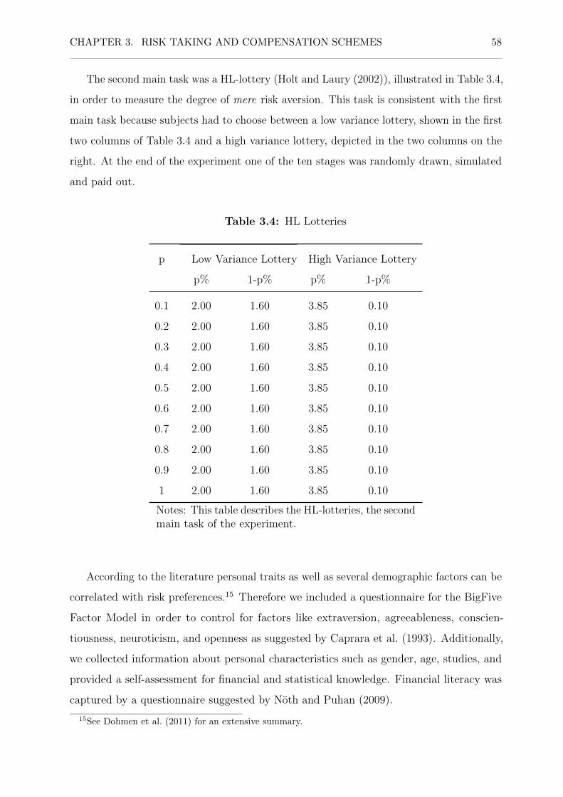
CHAPTER 3. RISK TAKING AND COMPENSATION SCHEMES 58
The second main task was a HL-lottery (Holt and Laury (2002)), illustrated in Table 3.4,
in order to measure the degree of mere risk aversion. This task is consistent with the first
main task because subjects had to choose between a low variance lottery, shown in the first
two columns of Table 3.4 and a high variance lottery, depicted in the two columns on the
right. At the end of the experiment one of the ten stages was randomly drawn, simulated
and paid out.
Table 3.4: HL Lotteries
p Low Variance Lottery High Variance Lottery
p% 1-p% p% 1-p%
0.1 2.00 1.60 3.85 0.10
0.2 2.00 1.60 3.85 0.10
0.3 2.00 1.60 3.85 0.10
0.4 2.00 1.60 3.85 0.10
0.5 2.00 1.60 3.85 0.10
0.6 2.00 1.60 3.85 0.10
0.7 2.00 1.60 3.85 0.10
0.8 2.00 1.60 3.85 0.10
0.9 2.00 1.60 3.85 0.10
1 2.00 1.60 3.85 0.10
Notes: This table describes the HL-lotteries, the secondmain task of the experiment.
According to the literature personal traits as well as several demographic factors can be
correlated with risk preferences.15 Therefore we included a questionnaire for the BigFive
Factor Model in order to control for factors like extraversion, agreeableness, conscien-
tiousness, neuroticism, and openness as suggested by Caprara et al. (1993). Additionally,
we collected information about personal characteristics such as gender, age, studies, and
provided a self-assessment for financial and statistical knowledge. Financial literacy was
captured by a questionnaire suggested by Noth and Puhan (2009).
15See Dohmen et al. (2011) for an extensive summary.

CHAPTER 3. RISK TAKING AND COMPENSATION SCHEMES 59
The experiment was conducted via LIMESURVEY16 and took on average 25 minutes
to complete. 32 out of our pool of 161 subjects were randomly selected and earned 27.56
euros on average from all tasks.
3.6 Results
In this section, we present and discuss the results of our experiment and put them into
the context of the regulatory framework for executive remuneration in European financial
institutions.
3.6.1 Descriptive Results
Figure 3.3 illustrates the fraction of chosen high variance lotteries (Option B) per stage
(i.e., level of fixed salary). The ratio of subjects who choose Option B for the first two
stages is ten percent. This ratio rises (continuously) up to 54 percent in the last stage. The
proportion of subjects who switch from Option A to Option B per stage is quite constant
and lies between one and three percent. We removed 18 subjects out of 161 who switched
at least twice. We discuss their influence on the results in the following section.
There is a slump for a fixed salary of ten units. Nearly ten percent of our subjects
switch from Option A to Option B. As one can see in Table 3.2, this is the stage when
the fixed salary is higher than the highest possible outcome of Option A for the first time.
A DA averse decision maker with an RP determined by the fixed amount would receive
additional value because Option A only provides losses in the sense of the DA theory from
this stage on.
We perform a probit regression on the probability of choosing Option B and find no
significant influence of empirical factors (e.g., age or gender), all kinds of self-assessments
(statistical knowlegde, BIG5, risk preferences) and measures such as financial literacy or
preferences for consistency. This finding is in line with Gothmann and Noth (2015).
16www.limesurvey.com

CHAPTER 3. RISK TAKING AND COMPENSATION SCHEMES 60
Figure 3.3: Results: DA-Induced Risk Taking
6 7 8 9 10 11 12 13 14 15 16 17 18 19 20 21 22 23 24 25
Fraction of Chosen High Variance Lotteries
0.0
0.2
0.4
0.6
0.8
Notes: This figure illustrates the fraction of chosen high variance lotteries(Option B) per fixed salary.
This result contradicts EUT and the general assumption that individuals are risk averse
on average. Since we conducted a HL-lottery in order to control for risk preferences as
second main task of the experiment we can compare both results. Figure 3.4 illustrates
the fraction of chosen high variance lotteries per stage. Again, we removed 14 subjects
who switched at least twice (e.g., from Option A to Option B and back, see the following
section for a discussion).
A risk neutral decision maker should switch from Option A to Option B in the fifth
stage which is marked by the vertical line in stage five.

CHAPTER 3. RISK TAKING AND COMPENSATION SCHEMES 61
Figure 3.4: Results: Mere Risk Preferences
1 2 3 4 5 6 7 8 9 10
Fraction of Chosen High Variance Lotteries
0.0
0.2
0.4
0.6
0.8
1.0
Notes: This figure illustrates the number of chosen high variance lotteriesof the HL risk measure.
HL suggest a classification with regard to the degree of risk aversion based on the
number of chosen high variance lotteries as depicted in Table 3.5. This would imply that
our subjects are risk averse on average.17
17Gothmann and Noth (2015) conduct several mere and modified HL-lotteries. The authors reportsimilar results for their HL-lottery task.

CHAPTER 3. RISK TAKING AND COMPENSATION SCHEMES 62
Table 3.5: Degree of Risk Aversion
Number of Risky Choices Degree of Risk Aversion
9 -10 highly risk loving
8 very risk loving
7 risk loving
6 risk neutral
5 slightly risk averse
4 risk averse
3 very risk averse
2 highly risk averse
0-1 stay in bed
Notes: Classification of risk aversion according to Holt andLaury (2002), p: 1649
According to this classification, we compare the distribution of risk lovers for both
tasks: HL-lotteries and remuneration (main) task. Figure 3.5 depicts the results of both
lotteries. The left bar (Risk Loving (Main Task)) represents the fraction of subjects who
choose the high variance lottery of Option B for any stage. The right bar depicts the
fraction of subjects who revealed risk loving preferences.
We identify 11 percent risk lovers for the HL-task and 54 percent for the main task.
This finding is in line with Cole et al. (2015), who find that this behavior does not solely
depend on mere risk preferences. The authors conduct an experiment and can induce their
subjects to take risks by means of performance-based compensation schemes.
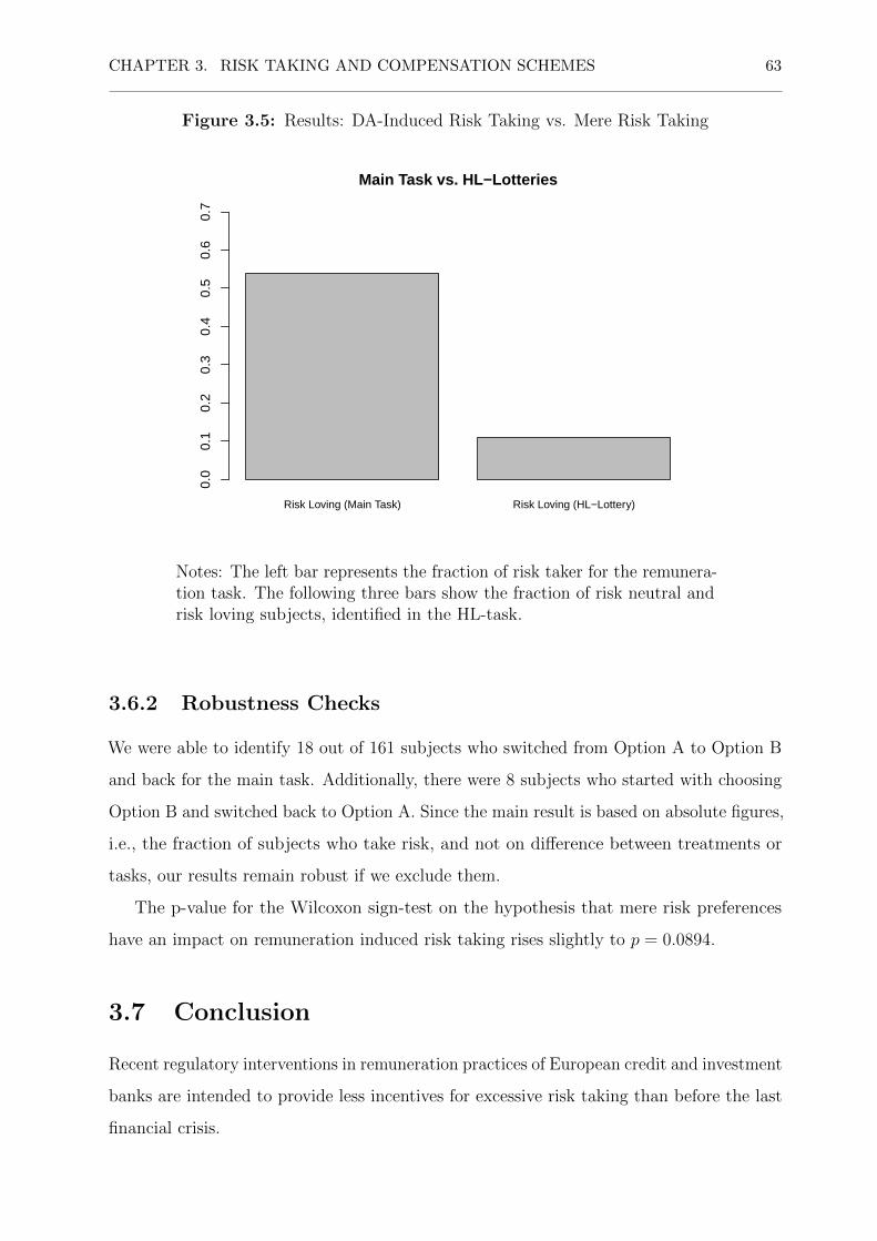
CHAPTER 3. RISK TAKING AND COMPENSATION SCHEMES 63
Figure 3.5: Results: DA-Induced Risk Taking vs. Mere Risk Taking
Risk Loving (Main Task) Risk Loving (HL−Lottery)
Main Task vs. HL−Lotteries
0.0
0.1
0.2
0.3
0.4
0.5
0.6
0.7
Notes: The left bar represents the fraction of risk taker for the remunera-tion task. The following three bars show the fraction of risk neutral andrisk loving subjects, identified in the HL-task.
3.6.2 Robustness Checks
We were able to identify 18 out of 161 subjects who switched from Option A to Option B
and back for the main task. Additionally, there were 8 subjects who started with choosing
Option B and switched back to Option A. Since the main result is based on absolute figures,
i.e., the fraction of subjects who take risk, and not on difference between treatments or
tasks, our results remain robust if we exclude them.
The p-value for the Wilcoxon sign-test on the hypothesis that mere risk preferences
have an impact on remuneration induced risk taking rises slightly to p = 0.0894.
3.7 Conclusion
Recent regulatory interventions in remuneration practices of European credit and investment
banks are intended to provide less incentives for excessive risk taking than before the last
financial crisis.

CHAPTER 3. RISK TAKING AND COMPENSATION SCHEMES 64
Our study focuses on a directive of the EU that requires credit and investments banks
to cap variable compensation to 100 percent of the fixed salary (2013/36/EU, article 94).
Based on studies of the EBA, we provide evidence that this rule led to a significant increase
of fixed salaries on average.
Motivated by insights provided by Cole et al. (2015) that performance (i.e., risk) based
compensation schemes can induce a biased perception of risks and thus excessive risk taking,
we are interested in the question of whether this change in the structure of remuneration
schemes has an impact on individual risk taking.
We conduct a risk taking experiment and show that more than half (54 percent) of
our subjects reveal EUT-inconsistent choice behavior. By gradually increasing the fixed
component of their total compensation, subjects switch from choosing a low variance lottery
to a high variance lottery. Our results indicate that regulatory initiatives such as a bonus
cap might induce bank managers to take on more risks instead of less.
Agreeing with Admati and Hellwig (2014), we recommend further research on the
question whether simple rules (i.e., heuristics) can provide more robustness and less
incentives for regulatory arbitrage such as the proposal of Bebchuk (2009) who suggests to
fix bankers’ pay.

CHAPTER 3. RISK TAKING AND COMPENSATION SCHEMES 65
References
Abeler, Johannes, Armin Falk, Lorenz Goette, and David Huffman (2011). “Reference
Points and Effort Provision”. American Economic Review, 470–492.
Admati, Anat and Martin Hellwig (2014). The Bankers’ New Clothes: What’s Wrong with
Banking and What to Do About It. Princeton University Press.
Bebchuk, Lucian (2009). “Fixing Bankers’ Pay”. Economists’ Voice 6(11).
Bebchuk, Lucian A and Jesse M Fried (2009). Pay Without Performance: The Unfulfilled
Promise of Executive Compensation. Harvard University Press.
Bell, David E (1985). “Disappointment in Decision Making under Uncertainty”. Operations
Research, 1–27.
Bouwman, Christa HS and Ulrike Malmendier (2015). “Does a Bank’s History Affect Its
Risk-Taking?” American Economic Review 105(5), 321–325.
Caprara, Gian Vittorio, Claudio Barbaranelli, Laura Borgogni, and Marco Perugini (1993).
“The ’Big Five Questionnaire’: A New Questionnaire to Assess the Five Factor Model”.
Personality and Individual Differences 15(3), 281–288.
Charness, Gary, Uri Gneezy, and Alex Imas (2013). “Experimental Methods: Eliciting Risk
Preferences”. Journal of Economic Behavior & Organization 87, 43–51.
Cole, Shawn, Martin Kanz, and Leora Klapper (2015). “Incentivizing Calculated Risk-
Taking: Evidence from an Experiment with Commercial Bank Loan Officers”. Journal
of Finance 70(2), 537–575.
Dittmann, Ingolf, Ernst Maug, and Oliver Spalt (2010). “Sticks or Carrots? Optimal CEO
Compensation When Managers Are Loss Averse”. Journal of Finance 65(6), 2015–2050.
Dohmen, Thomas, Armin Falk, David Huffman, Uwe Sunde, Jurgen Schupp, and Gert G
Wagner (2011). “Individual Risk Attitudes: Measurement, Determinants, and Behavioral
Consequences”. Journal of the European Economic Association 9(3), 522–550.
EBA (2016). Benchmarking of Remuneration Practices at Union Level. Tech. rep. European
Banking Authority.
Eisenfuhr, Franz, Martin Weber, and Thomas Langer (2010). Rational Decision Making.
Springer.

CHAPTER 3. RISK TAKING AND COMPENSATION SCHEMES 66
European Banking Authority (2014). Benchmarking of Remuneration Practices at Union
Level. Tech. rep. European Banking Authority.
Fahlenbrach, Rudiger, Robert Prilmeier, and Rene M Stulz (2012). “This Time Is the
Same: Using Bank Performance in 1998 to Explain Bank Performance During the Recent
Financial Crisis”. Journal of Finance 67(6), 2139–2185.
Fehr-Duda, Helga and Thomas Epper (2012). “Probability and Risk: Foundations and
Economic Implications of Probability-Dependent Risk Preferences”. Annu. Rev. Econ.
4(1), 567–593.
Ferri, Fabrizio and Robert F Goex (2013). “Regulation and Disclosure of Executive
Compensation”. European Accounting Review 22(1).
Financial Stability Board (2009). Basel.
Friend, Irwin and Marshall E Blume (1975). “The Demand for Risky Assets”. American
Economic Review, 900–922.
Gothmann, Roger and Markus Noth (2015). “Risk Taking and Induced Reference Points”.
Working Paper.
Gul, Faruk (1991). “A Theory of Disappointment Aversion”. Econometrica, 667–686.
Harrison, Glenn W and Elisabet E Rutstrom (2008). “Risk Aversion in the Laboratory”.
Research in Experimental Economics 12, 41–196.
Holt, Charles A and Susan K Laury (2002). “Risk Aversion and Incentive Effects”. American
Economic Review 92(5), 1644–1655.
Kahneman, Daniel and Amos Tversky (1979). “Prospect Theory: An Analysis of Decision
under Risk”. Econometrica, 263–291.
Koszegi, Botond and Matthew Rabin (2007). “Reference-Dependent Risk Attitudes”.
American Economic Review 97(4), 1047–1073.
Lefebvre, Mathieu and Ferdinand M Vieider (2014). “Risk Taking of Executives under
Different Incentive Contracts: Experimental Evidence”. Journal of Economic Behavior
& Organization 97, 27–36.

CHAPTER 3. RISK TAKING AND COMPENSATION SCHEMES 67
Lonnqvist, Jan-Erik, Markku Verkasalo, Gari Walkowitz, and Philipp C Wichardt (2015).
“Measuring Individual Risk Attitudes in the Lab: Task or Ask? An Empirical Compari-
son”. Journal of Economic Behavior & Organization 119, 254–266.
Malmendier, Ulrike and Geoffrey Tate (2005). “CEO Overconfidence and Corporate Invest-
ment”. Journal of Finance 60(6), 2661–2700.
Noth, Markus and Tatjana Puhan (2009). “How to Hide Mutual Fund Fees–Experimental
Evidence”. Working Paper.
Ockenfels, Axel, Dirk Sliwka, and Peter Werner (2014). “Bonus Payments and Reference
Point Violations”. Management Science 61(7), 1496–1513.
Prendergast, Canice (1999). “The Provision of Incentives in Firms”. Journal of Economic
Literature, 7–63.
Prendergast, Canice (2000). “What Trade-Off of Risk and Incentives?” American Economic
Review, 421–425.
Uhde, Andre (2015). “Risk-Taking Incentives Through Excess Variable Compensation:
Evidence from European Banks”. Quarterly Review of Economics and Finance 60, 12–28.
Von Neumann, John and Oskar Morgenstern (1947). “The Theory of Games and Economic
Behavior”.

Chapter 4
Asset Management of GermanFoundations
68

CHAPTER 4. ASSET MANAGEMENT OF GERMAN FOUNDATIONS 69
4.1 Introduction
According to the Bundesverband Deutscher Stiftungen (2015), there were more than
21,300 foundations (BGB companies) in Germany at the end of 2015, whereof 95 percent
exclusively and directly pursue non-profit and/or charitable objectives (here: non-profit) in
the sense of §52 Abs. 1 S. 1 Abgabenordnung (AO). This norm stiulates that a foundation
pursues non-profit objectives if and only if its activities are aimed at supporting the public
on a material, mental or ethical level in an altruistic, exclusive and immediate way.1
Half of these foundations had been founded in the last 14 years (Wigand et al. (2015)).
In total, they manage assets of more than 100 billion euros (Bundesverband Deutscher
Stiftungen (2015)). Their expenditures amounted to 17 billion euros in 20142, whereof 5 bil-
lion euros resulted from current yields by their asset management activities (Bundesverband
Deutscher Stiftungen (2014b)).3
Given how plentiful the investment activities of German foundations are, we focus on
two questions. First, how should German foundations diversify their assets? Second, does
German foundation law imply investment behaviors of foundation managers that can lead
to welfare losses?
In Section 4.5, using stochastic simulations, we empirically estimate the welfare losses
of German foundations based on data ranging from 2003 to 2012.
Our study is motivated by Huttemann and Schon (2007). The authors highlight that
the German legal literature predominantly defines asset management for foundations as an
instrument for risk avoidance with a focus on safe and steady incomes.4
The focus of our considerations lies on small and mid-sized foundations (assets under
management < 10, 000, 000 euros). We opt for this group because it is representative for
nearly 95 percent of all foundations registered in Germany and represents up to 70 percent
of the overall assets of all foundations (i.e., 70 billion euros). Furthermore, this group
does usually not operate with a professional in-house asset management (Bundesverband
1For a history of German foundation law see Schauhoff (2010) who states the term ’gemeinnutzig’ wasfirst mentioned at the end of the 18th century in the Preußisches Allgemeines Landrecht. According tothat the management and the application of individual property was legally privileged as far as it wasapplied to promote the ’gemeinschaftlichen Besten der Gesellschaft’.
2These expenditures equate nearly six percent of the budget expenditures of the Federal Republic ofGermany in 2014 (296,5 billion euros according to the Haushaltsgesetz 2014)
3One should mention that the cumulative property of all German foundations mentioned above ismainly based on book values. Thus, the relation of the cumulative property and total spendings fromcurrent yields is actually lower than five percent.
4See also Seifart et al. (2013) and Reuter (2012).

CHAPTER 4. ASSET MANAGEMENT OF GERMAN FOUNDATIONS 70
Deutscher Stiftungen (2014a)).
Our research question is closely linked to a persistent key obstacle that is widely
discussed in scientific and practical studies: what is the optimal asset allocation?5
Such an optimal allocation must serve the following purposes: the sustainable preser-
vation of assets and the generation of adequate current income in order to carry out the
foundation’s predefined goals. The main (practical) problem for the German non-profit
sector is the still existing uncertainty about the questions which asset classes and asset
allocations are covered by the German foundation law and what the guidelines of an efficient
asset management strategy have to be derived from these norms (e.g., Huttemann and
Schon (2007) or Schroder (2010)).
Therefore, we start with the definition of a legal and financial framework for German
foundations in the first two sections of this study. We do so by evaluating the current
legal literature as well as court rulings in Section 4.2 and derive and discuss possible legal
restrictions as one part of our legal and financial framework.
In Section 4.3, we discuss asset management strategies suggested by the literature. The
main focus of this part of the framework lies on easy to implement and robust asset allocation
strategies as suggested, for instance, by Jacobs et al. (2014) or Duchin and Levy (2009).
The authors compare robust and easily implementable asset management strategies with
different Markowitz-otimized portfolios and conclude that these sophisticated optimizations
have no significant advantage compared to simple heuristics, such as 1N
-strategies. These
studies are part of a current body of literature which find analytical and empirical evidence
that a wide range of simple decision rules can provide more robust returns than complex
optimization models.6
To the best of our knowledge, there are no studies which combine legal and financial
research in order to define an integrated framework for the asset management of German
non-profit foundations. Schroder (2010) upon touches this area by proposing suitable asset
classes for German foundations but lacks a concise strategy for their portfolio optimization.
The starting point of such an investigation should be an appropriate and specific
measure for risk. We base our study on the corresponding considerations of Schroder (2010).
Taking these suggested measures into account (risk-adjustment) we can show that a focus
5In this study we assume a foundation which tries to achieve its purpose(s) through autonomouslygenerating capital gains from the foundation capital. Thus, we do not take additional capital flows such asexternal donations or endowment contributions into account.
6See DeMiguel et al. (2009) for a comprehensive overview.

CHAPTER 4. ASSET MANAGEMENT OF GERMAN FOUNDATIONS 71
on short-term and downside volatility can lead to inefficient asset allocations, which can be
empirically observed. Once we have derived the legal and financial framework, we compare
different empirical asset allocations with the suggested strategies (i.e., heuristics) by means
of Monte Carlo simulations in Section 4.5.
We find that empirical asset allocation policies can be dominated by simple heuristics
with regard to all risk measures. Thus, we provide evidence that empirical asset allocations
can generate welfare losses of 40 to 90 percent of their (actual) returns due to asset
management strategies with a focus on exaggerated risk avoidance.
4.2 Institutional (Legal) Framework
In this chapter, we discuss and derive a legal framework for the asset management of
German non-profit foundations. We start with a description of the German foundation law,
consisting of federal legislation plus the 16 separate laws on foundations of the German
federal states. Since laws are usually subject to interpretation, we then provide an overview
of relevant court rulings and their potential consequences.
4.2.1 German Foundation Law
Foundations are statutory corporations (§80 Abs. 1 Buergerliches Gesetzbuch (BGB)). In
this section, we discuss relevant legal restrictions for the asset management of German
foundations.7
Beside the distinction between federal law and that of the federal states, one can
distinguish between civil and public foundation law. The civil legal framework is defined
by §§80-88 BGB and §93 AktG. Within this range, the 16 federal state laws can further
specify this framework.8 The public law is defined in §§51-68 Abgabenordnung (AO). A
differentiation between public and civil law is relevant because it implies different regulatory
7At this point one should mention, that the founder is authorized to determine the guidelines for theasset allocation within the foundation’s statute. An example is the Alfred Toepfer Stiftung F.V.S. inHamburg. In its statute, article 6 establishes that funds are to be invested into real estate and landedproperty in Europe. It is recommended to waive such requirements within the foundation statutes, becausesubsequent modifications are hardly possible since they would violate the founders intention in principle.Thus, guidelines for the asset management should be outsourced into investment policies. Particularattention should be paid to the fact that capital markets are subject to financial innovations. Thus,investment guidelines should be flexible enough to leave scope of action.
8In the case of contradictory federal and federal state regulations there is the principle that federal lawtakes precedence over state law according to article 31 of the constitution (Grundgesetz).

CHAPTER 4. ASSET MANAGEMENT OF GERMAN FOUNDATIONS 72
authorities, which will be discussed in the following three sections.
Germany’s civil and public law for foundations provides two important guidelines for the
asset management of German foundations. While the civil law is focused on the question to
what extent a foundation manager has to maintain the original endowment, the public law
incorporates restrictions on the use of current income (e.g., dividends interest payments)
and the redistribution of funds between different asset classes.
Federal Civil Law (BGB)
The majority of the federal civil foundation law is laid down in §§80-88 BGB, which is
supplemented by §93 AktG. According to §80 Abs. 2 S. 1 BGB a foundation is given
legal endorsement if and only if the foundation is able to fulfill its goals in a sustainable
manner.9
Schauhoff (2010) concludes that §80 BGB does not provide concrete recommendations for
actions regarding the asset management of foundations. At the same time Huttemann and
Schon (2007) interpret this norm as the specification for the preservation of the endowment.
The authors substantiate this main principle by emphasizing that the endowment must
be invested efficiently and safely. Falk (2011) adds to this interpretation and argues that
a foundation requires steady earnings in order to satisfy the intention of the founder,
respectively of §80 Abs. 2 S. 1 BGB. Thus, one can summarize that §80 Abs. 2 S. 1 BGB
constitutes two regulatory major principles of German foundation law: (1) the sustainable
preservation of the endowment and (2) the generation of revenues in order to permanently
fulfill the foundation’s purposes.10
Theuffel-Werkhahn and Siebert (2013) define the restrictions for an asset manager
negatively. Following their interpretation, the endowment must not completely invested in
one type of assets only – neither in single stocks nor in saving accounts. Both strategies
would violate the principles of precaution and economic efficiency which the authors derive
from §80 Abs. 2 S. 1 BGB.
According to §93 Abs. 1 AktG, the so-called ’business judgment rule’ has to be applied
for managers of non-profit foundations as well. Organs (i.e., asset managers) of a foundation
cannot be made liable for losses incurred if the have carefully considered all necessary
9§80 Abs. 2 S. 2 BGB defines an institution whose endowment can be used up (non-perpetual trust).The consumption of the endowment must be ensured for at least 10 years.
10The wording of §80 BGB is provided in Section A.3.1 of the Appendix.

CHAPTER 4. ASSET MANAGEMENT OF GERMAN FOUNDATIONS 73
information. Thus, according to §93 Abs. 1 AktG investments in a basket of single stocks
selected by the foundation manager could violate the business judgment rule if the manager
does not thoroughly analyze all available information about every single corporation that
is being invested in. According to §93 Abs. 1 AktG one might argue that an investment
in a basket of single assets (i.e., single stocks or single bonds) instead of broader based
indices is subject to comprehensive documentation requirements.
Considering these interpretations of the federal civil law, one can summarize that
extreme asset allocations would violate §80 Abs. 2 S. 1 BGB. Examples for extreme
allocations could be investments which generate no revenues (e.g., precious metals) or
would be speculative (e.g., single stock(s)).
Federal State Civil Law (Landesstiftungsgesetze)
The explicit statutory requirements regarding the principle of preservation of assets are
stipulated in the foundation laws of the sixteen German federal states. These rules can be
divided into four degrees of preservation as summarized in Table 4.1.
These degrees of preservation range from: ’the assets shall be kept undiminished on
a permanent basis’11 which obviously requires the preservation of assets in real terms, to
’the assets of the foundation must be maintained unimpaired if possible’12, which provides
a wide scope of action for the foundation’s management. The majority of the federal
state foundation laws contain the following wording: ”the assets must be contained or
contained unimpaired”, which both can be interpreted as the preservation of assets in
nominal terms (e.g., Reuter (2012)). Nevertheless, there is an ongoing and still open debate
in the literature on the question whether one can interpret the term ’unimpaired’ as ’in
real terms’ or ’in nominal terms’ (e.g., Huttemann (2014)).
According to this debate, one can find indications for the legislator’s intentions when
analyzing the introductory laws of the foundation laws of Hamburg and Sachsen-Anhalt.
Both regulations suggest maintaining the foundation’s assets in real terms.13
The legal literature (e.g., Huttemann and Schon (2007)) directly derives from these
principles that the assets of the foundation must be sufficiently diversified. We will
11§4 Abs. 3 foundation law Saxonia (August 7, 2004)12e.g., §4 Abs. 2 foundation law Hamburg (December 14, 2005)13The sample statute which is provided by the foundation supervisory authority in Ham-
burg even explicitly contains this requirement (see §3 Abs. 3 sample statute Hamburg(http://www.hamburg.de/justizbehoerde/stiftungen/4125446/downloads/)).

CHAPTER 4. ASSET MANAGEMENT OF GERMAN FOUNDATIONS 74
analyze and complement this abstract legal interpretation from a financial point of view in
Section 4.3 since this strand of literature does not provide any concrete guidelines for asset
management. The focus of the following financial investigation, therefore, is the question:
how should a foundation diversify its assets?14
Table 4.1: Preservation Principles of the German Federal States
Scope of the Principle of Endowment
Preservation
Federal State
The assets of the foundation must
be maintained.
Baden-Wurttemberg, Sachsen-
Anhalt, Schleswig-Holstein, Thurin-
gen
The assets of the foundation must be
maintained in an unimpaired way.
Bayern, Berlin, Bremen, Hessen,
Niedersachsen, Nordrhein-Westfalen,
Saarland
The assets of the foundation must
be maintained in an unimpaired way
if possible.
Hamburg, Rheinland-Pfalz
The assets shall be kept undimin-
ished on a permanent basis.
Sachsen
No guidelines Brandenburg, Mecklenburg-
Vorpommern
Notes: This table is based on an evaluation of the Landesstiftungsgesetze of all Germanfederal states. A German translation of the original passages can be found in Section A.3.2of the Appendix. The relevant articles are provided in Section A.3.3.
14The RAG-foundation which is one of the largest foundations in Germany has a slightly diversifiedportfolio of assets. The foundation maintained assets of more than 18 billion euros at the end of 2014.With an interest of 67.9 percent the foundation is the largest stockholder of the Evonik group (ISINDE000EVNK013), which corresponds with nearly 45 percent of the foundations endowment.

CHAPTER 4. ASSET MANAGEMENT OF GERMAN FOUNDATIONS 75
Most federal state foundation laws include additional principles for the organization
of foundations asset management. These statements do not provide any clarifications for
the operational asset management since they primarily clarify that the foundation’s assets
must be managed economically (Schroder (2010)).

CHAPTER 4. ASSET MANAGEMENT OF GERMAN FOUNDATIONS 76
Public Law (Fiscal Code)
According to §5 (1) number 9 KStG, non-profit foundations are exempt from taxes on
income as far as they comply with the requirements of §§51-68 AO.15
The Fiscal Code contains no explicit guidelines about the question whether a foundation
can lose the privilege of tax exemption in the case of a reduction of the original endowment.
The prevailing view in the literature is that a decline of the original endowment caused by
the asset management will generally not lead to foundations having their tax exemption
revoked (e.g., Theuffel-Werkhahn and Siebert (2013), Falk (2011)).
The authors summarize that as far as the foundation operates a taxable economic
business, losses of this section (i.e., commercial sphere) may not be compensated by funds of
the non-material sphere.16 The German Fiscal Code17 provides explicit provisions regarding
the management and the use of the property of the foundation.
First, we investigate the principle of the commitment of assets laid down in §55 (1)
number 1 and number 4 AO. Therefore, funds of the foundation may only be used for
purposes laid down in the statutes. Nevertheless, a foundation can only plow back profits
in a restrictive manner. §55 (1) number 5 AO has a concrete and direct effect on the
operational asset management. According to that central rule, the current income of
a foundation has to be spent within the following year of the fund’s inflow, exclusively
usable for the foundation’s purposes only (obligation of expenditure).18 This also includes
donations. Excluded from this principle is regular income from investments (i.e., interests,
dividends). Not more than one third of the income from investments can be used to set
aside as a free reserve (§62 (1) number 3 AO), i.e. for the preservation of the foundation
endowment (in real terms). Additionally, gains realized from shifts can be placed in a
restructuring reserve (Note 27 of the Fiscal Code Application Decree19 regarding §55 AO ).
Table 4.2 summarizes the legal options to transfer funds from one sphere of the
foundation to another. This is relevant for the original endowment, reserves and current
income. Free reserves and restructuring reserves are legislative vehicles to transfer current
15The tax exemption for revenues does not capture Value Added Tax, since there is no statutory provisionfor non-profit institutions by the Value Added Tax Act.
16The non-material sphere is the section of the foundation which is essential for the fulfillment of thefoundation purpose. The (taxable) commercial sphere has a unique purpose: generating revenues for thenon-material sphere (§14 AO).
17In German: Abgabenordnung (AO)18This implies an obligatory use of funds within a maximum of two years (if the inflow occurred on
January 1st)19In German: Anwendungserlass zur Abgabenordnung (AEAO)

CHAPTER 4. ASSET MANAGEMENT OF GERMAN FOUNDATIONS 77
Table 4.2: Legal Classification of Foundation Assets
Possible Financial Reserves
The Principle of :Preservation Locked Reserves Obligation of Expenditure
applies for:
original endowment free reserves current revenues⇔
additional endowment21 free reserves donations⇔
appropriated reserves restructuring reserves appropriated reserves
Notes: This table shows the classification of foundations reserves in their entirety as it isdefined in the German Fiscal Code (AO). By means of transfers or dissolution of reserves,funds can be transferred through all three possible legislative spheres (endowment, reservesand current revenues).
income to the endowment and vice versa. We will take this into account for the stochastic
simulations of our asset management strategies discussed in Section 4.3.6.
Additional flexibility for newly established foundations is provided by §62 (4) AO.
According to that rule, a foundation is authorized to transfer all of its revenues to the
endowment fund in the year of its founding and additionally in the following three legal
years.20
4.2.2 Current Jurisdiction
Particularly the question to what extent foundation managers can be held liable for losses
might have a significant effect on their willingness to take risks. Thus, we discuss the
relevant jurisdiction in order to define an operational framework. Huttemann and Schon
(2007) analyze three court decisions of the Bundesfinanzhof (BFH).22 23 24 We extend this
survey with current rulings of the previous years.
According to Huttemann and Schon (2007), it can generally be assumed that the BFH,
as well as the Bundesgerichtshof (BGH), do not take a decline in the assets of a foundation
20Since we do not distinguish between newly established and longer existing foundations for purposes ofour study, we do not take this rule into account. Furthermore, §62 (4) AO obviously does not alleviate theproblem of the preservation of assets by the admission to increase the original endowment.
21The principle of preservation does not apply for additional endowments if the founder has explicitlyexcluded his/her additional endowment from this principle.
22BFH v. 2.10.1968 I R 40/68 BFHE 93, S.522 ff.23BFH v. 13.11.1996 I R 152/93 BStBl II 1998, S. 711 ff.24FG Munster v. 10.12.2001 9 K 2537/98 K (juris)

CHAPTER 4. ASSET MANAGEMENT OF GERMAN FOUNDATIONS 78
as an occasion to state a breach of public foundation law. However, there are cases when
a foundation manager can be held responsible for losses of the asset management. We
identify two elements of these cases by evaluating the relevant court decisions, summarized
in Table 4.3. The first one, in line with the findings of Huttemann and Schon (2007), is a
compensation of losses which were generated by the commercial sphere with funds of the
non-material sphere. A commercial sphere can be established by investments which require
an active management (Reuter (2012)). This could be the case, for instance, for direct
investments in real estate due to the need of property and facility management (active
management).
The other fundamental principle, one can derive from the latest jurisdiction, is that
foundation managers cannot be held liable for losses caused by their asset management
strategy if the have administered a sufficiently diversified portfolio of suitable assets. Thus,
we will analyze this principle in the second part of our investigation (financial framework),
taking as a starting point recent research on diversification strategies.

CHAPTER 4. ASSET MANAGEMENT OF GERMAN FOUNDATIONS 79
Table 4.3: German Court Decisions Regarding the Asset Management of German Foun-dations
Court Guiding Principle(s) Implications for Asset Management
BFH (13.11.1996IR 152/93)
A loss which was generated out of thenon-material sphere is not allowedto be compensated by funds of thenon-material sphere.
Certain asset classes such as privateequity are usually assessed as com-mercial activies by the German fiscalauthorities (Reuter (2012)). Theseinvestments usually start with lossesin the first periods25, so that thisinvestment class is not suitable asa single investment and should bepooled.
BGH (22.03.2011XI ZR 33/10)
A derivative (i.e., interest rate swap)by itself is a bet.
The BGH highlights that a bankadviser has to document whether aswap does match with the risk pro-file of a town council. The customermust be informed that such an as-set is a bet. The classification ofa mere swap as speculation by theBGH might induce that a derivativeby itself 26 is not an appropriate assetfor a foundation.
OLG Oldenburg(8.11.2013 6 U50/13)
A foundation manager is liable tomake compensations for a loss in-duced by a higher than allowed stockexposure and a long period of losseswithout any adjustments27
The court assessed a breach of dutyconcerning a higher than permittedstock exposure. In addition, this de-cision implies that the foundation’sassets must be diversified sufficiently.
BGH (20.11.2014III ZR 509/14)
This verdict confirms OLG Olden-burg (08.11.2013 6 U 50/13)28
FG Munster(11.12.2014 3 K323/12 Erb)
A portfolio which includes 70 percentloans, granted to corporations whichcan not exhibit an investment grade,implies a contravention
The court recognizes that a low in-terest level requires a higher willing-ness to take risks in order to gener-ate earnings for the mission of thefoundation. However, 70 percentgranted loans is defined as a clusterrisk which is too high.
OLG Frankfurt(28.01.2015 1 U32/13)
1. Foreign currency leveraged closedproperty funds29 are not suitable fora German foundation
The court did not separate the closedproperty funds from the foreign cur-rency loan. Thus, one can imply thatat least foreign currency loans are aviolation of the foundation law.
2. Bonds with a fixed rate ofinterest30 are safe investments andsuitable for a German foundation inorder to preserve the property.
A foundation portfolio of 100 percent(investments grade) bonds is not aviolation of the foundation law.

CHAPTER 4. ASSET MANAGEMENT OF GERMAN FOUNDATIONS 80
4.2.3 Summary of Relevant Legal Restrictions
Based on current legal norms and court decisions, the main restrictions for the asset
management of German foundations can be summarized as follows: Asset classes which
can involve commercial activities such as closed real estate funds or direct investments in
private equity are not suitable assets since they can cause losses which are not allowed to
be compensated by the funds of the non-material sphere. Furthermore, assets which imply
a bet, such as swaps or stocks of virtually insolvent companies (i.e., penny stocks) do not
align with the purposes of German foundations.
Extreme asset allocations can represent an infringement of the principle of preservation.
This could be, for instance, a portfolio with 100 percent commodities or 100 percent
liquidity whereas foundation portfolios including 100 percent bonds or 100 percent stocks
seem to be authorized under the German foundation law. Nevertheless, a foundation
manager can be held liable for losses due to a poorly diversified asset allocation. Thus, the
presentation and discussion of suitable diversification approaches is subject of the following
section (financial framework).
4.3 Financial Framework
In this section, we discuss suitable asset management strategies for German foundations,
given the legal framework we defined for the institutional (legal) framework before.
As derived in the preceding sections, there is one legal principle which has already been
confirmed by German courts: a foundation manager cannot be held responsible for losses
if the foundations assets are sufficiently diversified. Therefore, it is the objective of this
part of our study to discuss suitable diversification strategies.
By means of stochastic simulations we compare empirical asset management strategies
with strategies suggested by the (recent) literature. This analysis will provide us with
information for our second research question: can the actual (empirical) investment
behavior of German foundation managers lead to welfare losses? We start with an analysis
26So-called J-curve effect27The assets of the foundation had fallen from 8.84 m euros in 2001 to 2.55 m euros in 2008. The
manager was sentenced to reimburse 1.128 m euros.28The BGH increased the claim for reimbursement by about 330,000 euros.29In this case a German bank had suggested to invest into a closed property funds. This investment was
financed by a loan in CHF due to the fact that the interest level in Switzerland was lower than in Germany.30One can imply that the court refers to investment grade bonds.

CHAPTER 4. ASSET MANAGEMENT OF GERMAN FOUNDATIONS 81
of empirical studies about the investment behavior of German foundations.
4.3.1 Empirics
In order to define an empirical benchmark for our stochastical simulations, we start by
analyzing the empirical asset management strategies of German foundations. We narrow
our focus further down to German foundations with assets under management of less than
10 million euros. According to the Bundesverband Deutscher Stiftungen (2014c) this class
is representative for nearly 95 percent of all registered German foundations, as can be
seen in Figure 4.1. These foundations have in common that they usually do not have a
professional in-house asset management.31 Thus, they are not subject to any requirements
to publish financial statements. Representative information about their asset allocations
and methods of portfolio management are rare.
Figure 4.1: German Foundation Properties in Classes
<100t−Euros <1m−Euros <10m−Euros <100m−Euros >1bn−Euros
frac
tion
0.0
0.1
0.2
0.3
0.4
0.5
0.6
Notes: This survey is primarily based on book values (BVDS(2014).
31Imagine a foundation with 10 million euros under management. If this foundation realized an annualreturn of 4 percent before costs it would have only 400,000 euros to distribute for charitable objectives andadministration (i.e., personnel) costs.
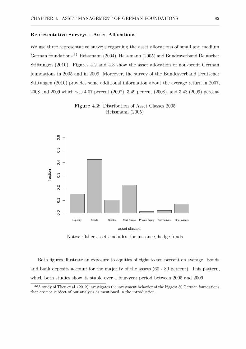
CHAPTER 4. ASSET MANAGEMENT OF GERMAN FOUNDATIONS 82
Representative Surveys - Asset Allocations
We use three representative surveys regarding the asset allocations of small and medium
German foundations:32 Heissmann (2004), Heissmann (2005) and Bundesverband Deutscher
Stiftungen (2010). Figures 4.2 and 4.3 show the asset allocation of non-profit German
foundations in 2005 and in 2009. Moreover, the survey of the Bundesverband Deutscher
Stiftungen (2010) provides some additional information about the average return in 2007,
2008 and 2009 which was 4.07 percent (2007), 3.49 percent (2008), and 3.48 (2009) percent.
Figure 4.2: Distribution of Asset Classes 2005Heissmann (2005)
Liquidity Bonds Stocks Real Estate Private Equity Deriviatives other Assets
asset classes
frac
tion
0.0
0.1
0.2
0.3
0.4
0.5
0.6
Notes: Other assets includes, for instance, hedge funds
Both figures illustrate an exposure to equities of eight to ten percent on average. Bonds
and bank deposits account for the majority of the assets (60 - 80 percent). This pattern,
which both studies show, is stable over a four-year period between 2005 and 2009.
32A study of Then et al. (2012) investigates the investment behavior of the biggest 30 German foundationsthat are not subject of our analysis as mentioned in the introduction.

CHAPTER 4. ASSET MANAGEMENT OF GERMAN FOUNDATIONS 83
Figure 4.3: Distribution of Asset Classes 2009BVDS (2010)
Bonds Stocks Real Estate other Assets
asset classes
frac
tion
0.0
0.1
0.2
0.3
0.4
0.5
0.6
Notes: Other assets includes liquidity, private equity, hedgefunds and derivatives
How do German Mutual Funds for Foundations Diversify?
There are more than 39 open-end and exchange traded funds for German foundations
according to a study of Haake (2013). Thus, one could analyze their investment strategies
in order to receive a proxy for the investment behavior of German foundations. However,
these funds represent only 4.3 billion euros under management. The largest fund, Deka
Stiftungen Balance33, has 1.4 billion euros under management.34 According to the key
investor information the fund’s management has to comply with the following guidelines:
an equity ratio up to a maximum of 30 percent and an investment focus on assets listed in
Euro.35
33ISIN DE000589686434The total issue surcharge is 2 percent and has running costs of 1.17 percent in 2014.35Source: https://www.deka.de/privatkunden/fondsprofil?id=DE0005896864

CHAPTER 4. ASSET MANAGEMENT OF GERMAN FOUNDATIONS 84
Empirical Implications and Benchmark
We have shown in the previous sections that German foundations on average mainly invest
in fixed incomes (i.e., government bonds). Schindler (2003) summarizes this behavior as
follows: a foundation manager can be held liable for losses only. In this context, Dimmock
(2012) finds evidence that university endowments with higher background risk invest more
in fixed income. Background risk is defined as the volatility of the foundation’s non-financial
income (e.g., donations). Moreover, assets listed in Euro are preferred.
We use the findings of the previous sections to derive our empirical benchmark. Due to
the heterogeneity of German foundations, a single asset allocation does not seem to be
appropriate and representative. Thus, our benchmark portfolios consist of an equity ratio
from 0 to 15 percent stocks and 85 to 100 percent bonds, both asset classes noted in Euro.
4.3.2 Literature – Asset Management for (German) Foundations
As we presented in detail before, in order to preserve the assets of the foundation, a
manager has to hold a sufficiently diversified portfolio. Our first research question implies
this, i.e., how should German foundations diversify, given the legal restrictions we derive
for the financial framework?
The literature on the question of how foundations should allocate their assets is
dominated by a US-centric perspective. However, the legal restrictions US and German
foundations have to adhere to differ significantly. A main difference is the obligation of
American foundations to spend five percent of their endowment per year. Another difference
is the restriction regarding potential asset classes. Whereas American foundations are
allowed to invest in nearly all asset classes, i.e., private equity, German foundations are far
more restricted in this respect.
The relevant literature on asset management can be divided into two strands. The first
one was established by Merton (1993). The author suggests the implementation of three
portfolios to preserve the foundation’s endowment in real terms: a market portfolio, a
risk-free interest rate portfolio, and a hedge portfolio. The function of the hedge portfolio
is to compensate for an inflation-caused increase of spendings for foundation goals. Rudolf
and Ziemba (2004) suggest complementing these portfolios by a liabilities hedge portfolio
in order to additionally hedge the foundations costs (e.g., administration costs). In this
context, Merton (1993) as well as Rudolf and Ziemba (2004) recommend investing in assets

CHAPTER 4. ASSET MANAGEMENT OF GERMAN FOUNDATIONS 85
that are negatively correlated with the liabilities, respectively expenditures.
As the small foundations we focus on are usually unable to manage rather complex
hedge portfolios, this strand of literature is of limited use for our analysis. Thus, we choose
another approach that is based on a second strand of literature, which compares static and
dynamic value protection strategies.
Dybvig (1999) and Bajeux-Besnainou and Ogunc (2006) show analytically that a
Constant Proportion Portfolio Insurance (CPPI) as suggested by Black and Jones (1987)
can theoretically outperform static strategies such as a protective put. This is in line with
Benninga and Blume (1985), who find evidence that static protection models (e.g., put
strategies) can be only utility maximizing in incomplete markets (e.g., the prohibition of
an investment in risk-free asset classes).
Under the restrictions of German foundation law, Schroder (2010) provides evidence by
means of stochastic simulations that CPPI-strategies cannot add additional value to the
results of simple buy and hold strategies.
Annaert et al. (2009) show analytically that CPPI can only add additional value under
very restrictive assumptions such as unconstrained borrowing, which a German foundation
is legally not allowed to comply with.
The major problem is determined by the design of such strategies and it is summarized,
for instance, by Choie and Seff (1989). Given a level of preservation (i.e., protection) of
the endowment, funds are shifted from a stock market portfolio (risky assets) to a riskless
portfolio should the value of the foundation portfolio fall short of the protection level
due to an increase of stock market volatility. Given the endless investment horizon of a
foundation, a fee-based protection method such as CPPI which smoothes out (short-term)
volatilities might be inappropriate for a German foundation. This assumption is in line
with Black and Perold (1992).36
For this reason, we solely focus on mere static approaches.
To the best of our knowledge there are no comprehensive studies about the question of
how German foundations should diversify their assets. In one of the rare contributions to
this topic, Schroder (2010) compares different static allocation methods (buy and hold)
between European and global stock and bond indices and finds no superior strategy.
36A modification of CPPI is the TIPP model (Estep and Kritzman (1988). In contrast to CPPI theprotection level in the TIPP model rises as the portfolio return increases. This additionally increases therisk, that the funds of the foundation are shifted into the risk-free asset without ever having the possibilityof participating in a recovery of the stock market.

CHAPTER 4. ASSET MANAGEMENT OF GERMAN FOUNDATIONS 86
In order to identify suitable allocation policies for German foundations, we continue
with the definition of portfolio selection criteria in the following section.
4.3.3 Performance and Risk Measures - Foundation Utility Op-
timization
The aim of the following sections is to identify diversification strategies that are suitable
for German non-profit foundations based on the literature discussed before. Thus, we
need selection criteria that reflect, among other aspects, the legal restrictions we derive in
section 4.2.
The primary legal criterion is the preservation of assets. This means that foundation
managers face an asymmetric risk as they can only be held liable for losses of the endowment.
In contrast, managers of mutual funds could also be called to account for a loss of profit
regarding their benchmarks.
Fishburn (1977) suggests for these purposes the so-called Lower Partial Moments, which
capture downside risks (i.e., the fall in value of the original endowment). As selection
criteria we choose the Lower Partial Moments of degree zero (LPM0), degree one (LPM1),
and degree two (LPM2), that are defined as follows:
LPM0 = E[(z − r)0], (4.1)
LPM1 = E[(z − r)1], and (4.2)
LPM2 = E[(z − r)2], (4.3)
with E as the expectations operator and r as observed (i.e., simulated) return and z as
target return. In cases where the foundations endowment must be preserved in real terms,
z must be greater than or equal to the rate of inflation. Equation 4.1 defines the lower
partial moment of degree zero (LPM0). This measure captures the frequency with which a
specific diversification strategy cannot reach the target return (i.e., inflation rate). LMP1
(Equation 4.2) quantifies the corresponding expected shortfall. The lower partial moment
of degree two (Equation 4.3) is a measure for the volatility below the target return. We

CHAPTER 4. ASSET MANAGEMENT OF GERMAN FOUNDATIONS 87
use all three lower partial moments as risk measures and potential selection criteria.
A risk averse decision maker (i.e., foundation manager) would choose an asset man-
agement strategy which provides her with the highest return per unit risk. Thus, for
conventional Markowitz optimization, the Sharpe Ratio (SR) (Sharpe (1966)) is usually
applied. The SR is a risk-adjusted performance measure that captures excess return per
unit risk and is defined as follows:
SR =r − zσ
, (4.4)
where σ is the standard deviation of the expected return r. Since volatility above the
target return z is not defined as risk for our purposes, we use a modification of the SR,
suggested by Sortino and Price (1994), the Sortino ratio (SoR), which is defined as in
Equation 4.5:
SoR =r − z√LPM2(z)
. (4.5)
The excess return is adjusted by the standard deviation below the target return.37 The
last selection criteria we use are the average current yield (CY) (e.g., dividends, coupons)
and the absolute growth (Growth)38 of the foundation’s assets, so that the optimization
problem for a German non-profit foundation is as follows:
Minimize LPM0, LPM1, LPM2,
and Maximize SoR, CY , Growth.
4.3.4 Potential Asset Classes
We complete the definition of a financial framework for German foundations with the
discussion of potential asset classes. Due to the scope of our research question, we do not
focus on liquidity management as well. Thus, liquidity is not an autonomous asset class
for our purposes.39
The German foundation law provides no clear guidelines which asset classes a foundation
manager is permitted to invest in. However, we have shown that investments which imply
37As can easily be seen, this is defined as the square root of the lower partial moment of degree two(LPM2).
38We assume a starting point of 100 euros for the purpose of the simulations.39For a study about the asset-liability management see Bajeux-Besnainou and Ogunc (2006).

CHAPTER 4. ASSET MANAGEMENT OF GERMAN FOUNDATIONS 88
commercial activities could be fraught with risks due to the legal prohibition of loss
compensation between the commercial and the non-material sphere. Therefore, we exclude
direct investments which could establish a commercial sphere.
As starting point we take asset classes Jacobs et al. (2014) recommend for (German)
private investors as shown in Table 4.4. With regard to the investment horizon, private
investors and foundations are not very different. Both institutions have a longer investment
horizon than institutional investors. Therefore, they do not have to focus on short-term
market movements. In contrast to stocks, Jacobs et al. (2014) argue that the currency risk
of bond portfolios needs to be controlled. That is why the authors restrict their analysis
to Euro-denominated bonds. Since our focus is on easy-to-implement asset management
strategies we follow their suggestion. The benchmark for each asset class is presented in
the third column.4041
Table 4.4: Asset Classes Suggested for Private Investors
Asset Class Region Benchmark
Stocks
Emerging Markets MSCI Emerging Markets
Eurozone EURO STOXX
North America MSCI North America
Pacific MSCI Pacific
Bonds Eurozone iBoxx Euro Overall
Commodities — S&P GSCI Commodity TR
Notes: Asset classes and benchmarks suggested for private investors by Jacobs et al. (2014).The authors recommend an allocation of 60 percent stocks (worldwide), 25 percent bonds(noted in Euro), and 15 percent commodities.There is no regional classification for commodities.
40The iBoxx Euro Overall is a capitalization-weighted index which contains government bonds andcorporate bonds from the Eurozone listed in Euro (source: http://www.markit.com/Product/IBoxx).
41The Euro Stoxx Index is a subset of the STOXX Europe 600 Index with large-, mid- and small-sizecompanies of 12 Eurozone countries (source: http://www.stoxx.com/index-details?symbol=SXXGT).

CHAPTER 4. ASSET MANAGEMENT OF GERMAN FOUNDATIONS 89
For a discussion of the fundamental suitability of the asset classes mentioned in Table 4.4
for the purposes of US or German foundations see Thaler and Williamson (1994) and
Schroder (2010). Commodities are not taken into account in these studies. We take this
class into consideration because Jacobs et al. (2014) find a slightly negative correlation with
bonds and equity. We find this effect with bonds as well. Figure 4.4 shows the Pearson
correlation coefficient for the asset classes discussed above for our estimation period (2003 -
2012).
From an ex-ante perspective, stocks are suitable for the diversification strategy of a
foundation for two reasons. First, they provide direct participation in the productive
capital which could thereby be a hedge against inflation. Second, dividends are current
yields that a foundation manager can immediately apply for statutory purposes.42
As our focus is on small and medium foundations, we do not consider direct real estate
investments. Such an investment could constitute a cluster risk. Schatz and Sebastian
(2009) and Sebastian et al. (2012) analyze to what extent Real Estate Investment Trusts
(REITs) could be a substitute for real estate. The authors show that especially for the long
run (i.e., periods longer than 30 years) REITs exhibit a higher correlation with real estate
than with stocks. For our estimation period we cannot find this effect in the data. This is
in line with the studies of Sebastian et al. (2012). For this reason, we exclude REITs.
One might argue that open-ended real estate funds could be a substitute for direct
real estate investments, too. We do not take these funds into account for their persistent
problems with their own liquidity management (e.g., Fecht and Wedow (2014)).
We also do not incorporate private equity since German foundations are restricted
to indirect investments in private equity. A direct investment could imply commercial
operations which are generally not authorized by the German fiscal authorities. For hedge
funds we could find no equivalent indices that satisfy the selection criteria suggested
by Jacobs et al. (2014). Additionally, in their analysis the authors conclude that the
diversification effect of alternative assets (i.e., hedge funds, private equity) is limited.
In view of the above we use the asset classes and corresponding indices as shown in
Table 4.5 for our stochastic simulations.
42See Wachter (2013) for an overview about the volatility of dividends.

CHAPTER 4. ASSET MANAGEMENT OF GERMAN FOUNDATIONS 90
Table 4.5: Overview: Time Series, 2003 –2012
Asset Class/Region Benchmark/Index Characteristics
Stocks
Emerging markets MSCI Emerging Markets Price and Total Return Index
Europe EURO STOXX Price and Total Return Index
North America MSCI North America Price and Total Return Index
Pacific MSCI Pacific Price and Total Return Index
Bonds
Europe iBoxx Euro Overall Price and Total Return Index
Other asset classes
Commodities S&P GSCI Commodity TR Total Return Index
Table 4.6: Descriptive Statistics for Asset Classes to be Considered (Estimation Period:2003–2012).
Asset class/ Interests-/Dividend- Price Total Standard
Region Payments Return Return Deviation
Stocks: regional indices
Emerging Markets 2.70% 9.67% 12.37% 20.35%
Europe 3.22% 0.50% 3.72% 22.08%
North America 2.00% 1.80% 3.80% 21.30%
Pacific 2.29% 1.33% 3.62% 20.26%
Bonds: Regional Indices
Europe 4.14% 0.46% 4.60% 3.23%
Commodities - - 0.61% 24.26%
Notes: Dividend- and interest-payments are measured by subtracting the return of theprice index from the return of the total return index.

CHAPTER 4. ASSET MANAGEMENT OF GERMAN FOUNDATIONS 91
Figure 4.4: Pearson Correlation of Relevant Assets
1 -0.23
1
-0.02
0.63
1
-0.3
0.6
0.22
1
-0.21
0.66
0.4
0.55
1
-0.25
0.49
0.13
0.51
0.77
1
BondEU
MSCIPA
GSCI
MSCIEM
MSCINA
EStoxx
BondEU
MSCIPA
GSCI
MSCIEM
MSCINA
EStoxx
-1.0 -0.5 0.0 0.5 1.0
PearsonCorrelation
Notes: Pearson correlation coefficients for relevant asset classes
4.3.5 Target Return and Interest Rates
The central parameter for our quantitative analysis is the target return. This parameter is
related to the question whether German foundations have to preserve their assets in real
or in nominal terms. The academic debate has come to the conclusion that a foundation is
obliged to aspire a perservation in real terms to avoid a lingering erosion of the profitability
and thus a reduced capability of sponsoring charitable objectives in a sustainable manner
(e.g., Reuter (2012)). Figure 4.5 shows the inflation rate for our estimation period in
relation to the risk-free interest rates.
As can be seen in the graph, the German inflation rate is quite volatile and ranges
between zero and three percent within the estimation period (2003 - 2012). However, we
choose a fixed rate of two percent as target return. We do this because expenditures of
German foundations are mainly determined by personnel expenses.43 For that reason we
do not take the price increase of a representative basket of commodities into account but
43According to the Bundesverband Deutscher Stiftungen 56.6 percent of German foundations purposeswhich are mainly driven by personnal costs (Bundesverband Deutscher Stiftungen (2014a)): 28.8 percentsocial purposes, 15.4 percent eduction, 12.4 percent science.

CHAPTER 4. ASSET MANAGEMENT OF GERMAN FOUNDATIONS 92
the increase of personnel expenses in Germany. According to the Hans Boeckler Stiftung,
German wage agreements add up to 2.08 percent per year over all branches from 2003 to
2012 (Boeckler (2013)).
Figure 4.5 also illustrates the interest-rate-inflation scenario the data for our Monte
Carlo simulations are estimated from.
Figure 4.5: Interest Rates, Price and Wage Inflation – 2003 - 2012
2004 2006 2008 2010 2012
−1
01
23
45
6
Real or nominal terms?
inte
rest
rat
es/in
flatio
n ra
te
InflationWage−InflationEuribor1MEuribor1Y
Notes: Short-term and medium-term interests are plot-ted against the average wage inflation rate and theinflation of German consumer prices.
4.3.6 Diversification Strategies
Carstensen (2003) (also Carstensen (1996)) shows, that mere money market strategies
cannot provide a preservation of assets. Thus, we do not take these strategies into account,
nor do we use them as benchmarks.44
With regard to the question of optimal asset allocation (i.e., diversification), there is
extensive literature on the comparison of sophisticated Markowitz optimization methods
with simple heuristics.
44This is unnecessary due to the construction of our risk and performance measures which include bydefinition the real interest rate as benchmark.

CHAPTER 4. ASSET MANAGEMENT OF GERMAN FOUNDATIONS 93
Several studies provide evidence, that simple decision rules like, for instance, 1N
can
provide superior and/or more robust results than a wide range of mean-variance (Markowitz)
models (e.g., Duchin and Levy (2009), DeMiguel et al. (2009), Tu and Zhou (2011) or
Jacobs et al. (2014)).45
In contrast, Kritzman et al. (2010) find evidence that optimized allocations can out-
perform equally-weighted portfolios. The authors argue that several studies showing the
opposite used samples that were too small. This criticism can be rejected by the work of
Jacobs et al. (2014), since the authors use market data from 1973 onwards. Furthermore,
they compare more than 500 heuristics with a wide range of Markowitz-models and come to
the conclusion that a stock market portfolio with the respective Gross Domestic Products
as weights for the stock market regions: Europe, Northern America, Emerging Markets
and Pacific can beat all Markowitz models.
Markowitz-optimized portfolio weights are sensitive to changes in the input parameters
that can be analytically derived (e.g., Poddig and Unger (2012)). According to Unger
(2015), this could have been one reason for the failure of these portfolios in the financial
crisis when events such as a breakdown of an investment bank tumbled previous correlations
and therefore the input parameters of existing risk models.46 As an outcome of the financial
crisis, the author highlights that by now, there are up to 17 definitions of robustness
regarding the sensitivity problem in the literature by.
For our purposes we focus on two: worst-case robustness and structural robustness
(Poddig and Unger (2012)). Worst-case robustness means that, for instance, in the case of
a market slump, the chosen diversification strategy will provide better results than other
possible strategies. Structural robustness stands for an insensitivity to the input parameters
(e.g., Unger (2015)). It is obvious that there is a trade-off and no single solution for this
problem. Nevertheless, we will take these considerations into account when comparing
different diversification strategies. Diversification heuristics as discussed in section 4.3.2
are at least structurally robust by their nature (i.e., 1N
or GDP-weighted).
Table 4.7 provides an overview of all diversification approaches (i.e., heuristics) we take
into account. A more detailed discussion of these models is given in the following sections.
45Another strand of literature is concernced with the fundamental problem of the statistical misinterpre-tation of results (e.g.,Ioannidis (2005) and Harvey et al. (2015).
46See Reinhart and Rogoff (2009) for a historical and financial analysis of the financial crisis.

CHAPTER 4. ASSET MANAGEMENT OF GERMAN FOUNDATIONS 94
Table 4.7: Diversification Approaches
A: Markowitz-Based Optimization
1 Minimum Variance Approach with Short Sales Constraints
B: Heuristic Models
2 Euro-Bonds with weights of 0 - 100 percent and GDP-weighted stock portfolio
(0-100 percent)
3 Euro-Bonds with weights of 0 - 100 percent and 1N
-weighted stock portfolio
(0-100 percent)
4 models 3 and 4 with a fraction of commodities instead of stocks (0 - 100)
percent)
Notes: This table summarizes the diversification methods we take into account for thestochastic simulations. Weights will be adjusted in steps of five percent.
Markowitz-based Approaches
Given the sensitivity problem discussed before, we focus on the Minimum-Variance (MV)
portfolio as the only representative for Markowitz-optimized portfolios. There is a strand
of literature which provides evidence that risk based optimized portfolios are worst-case
and structurally more robust than return-based approaches such as the Mean-Variance
framework (e.g., Allen (2010) and Lee (2011)).
Heuristics
For our purposes, the 1N
allocation of the equity component (e.g., Duchin and Levy (2009))
is the first diversification heuristic which has been extensively investigated. In the context
of this study, a 1N
allocation means that each geographic equity region (Europe, Northern
America, Emerging Markets, and the Pacific) is weighted equally (i.e., 14). However, Jacobs
et al. (2014) find evidence that their suggested GDP-weighted approach provides slightly
better results. Thus, we take both heuristics into account. In the sense of worst-case
robustness, a 1N
diversified portfolio might be more robust than a GDP-weighted one due
to an equal dependence on every stock region.47
47However, we are also aware of the fact the stock markets worldwide are by now highly correlated.

CHAPTER 4. ASSET MANAGEMENT OF GERMAN FOUNDATIONS 95
Rebalancing
Given a static allocation approach one has to decide how often the original asset weights
have to be rebalanced. According to Dichtl and Wambach (2014) neither too frequent
rebalancing nor infrequent rebalancing strategies are efficient due to a trade-off between
transaction costs and the advantage of the original asset allocation. The authors find
evidence that an adjustment to the initial weights once a year is an appropriate approach.
The same is suggested by Jacobs et al. (2014).
4.4 Quantitative Analysis
In this section, we discuss the technical aspects of our analysis and subsequently present
the results. The aim of our study is to test diversification strategies which we derived
in section 4.3.6 by means of stochastic simulations and the comparison with a range of
empirical benchmark portfolios. Subsequently, we want to find out whether there are
welfare losses due to inefficient diversification approaches, using a range of representative
empirical benchmarks.
4.4.1 Simulation Method and Design
We analyze and compare the diversification strategies suggested in section 4.3.6 by running
Monte Carlo simulations. These simulations generate continuously compounded portfolio
returns (d(lnS)), on the basis of a Geometric Brownian motion (Hull (2011)) which is
identical to the process Black and Scholes (1973) use for their option pricing model.
d(lnS) = (µ− σ2
2)dt+ σdz (4.6)
Since we use different assets for each diversification strategy that are more or less corre-
lated, we have to incorporate these correlations. We do this by a Cholesky-transformation
of the correlation matrix.48
We are aware of the fact that Monte Carlo simulations are based on the assumption of
idealized asset markets. This means that structural phenomena such as ”fat tails” and
autocorrelations are not incorporated into this model.49. In particular, by estimating the
48See, for example Poddig (2000) for a detailed discussion of this method.49See Detemple et al. (2003) for a detailled discussion.

CHAPTER 4. ASSET MANAGEMENT OF GERMAN FOUNDATIONS 96
input parameters from historical data (expected returns, volatilities, and corresponding
correlations of the asset classes), the choice of the estimation period has a substantial
influence on the results of the simulations. Nevertheless, Monte Carlo simulations are still
an appropriate means for the simulation of asset prices (e.g., Detemple et al. (2003)). The
mentioned weaknesses are reduced by the choice of a suitable estimation period (basic
scenario) and by a large set of robustness checks. In most studies, these robustness checks
include the separation of the basic scenario into subscenarios which makes it possible to
investigate the influence of specific events on the results.
We estimate the input parameters for our basic scenario from 1 January 2003 to 31
December 2012. As can be seen in the upper graph of Figure 4.6 this period includes two
significant price drops in the stock market. The first market slump coincides with the
announcement of the insolvency of Lehman Brothers Holding Inc. in 2008 which marked
the first escalation of the financial crisis. The second decline in 2011 took place after a
potential exit of Greece from the Eurozone had been announced. Furthermore we exclude
years before 2003 for two reasons. First, the period of 2001 - 2002 is mainly characterized
by an additional market slump: the meltdown of the so-called New Economy. Second,
before the introduction of the Euro, European investors were faced with extensive currency
risks. We also do not consider years after 2012 because since then, particularly bond yields
are being being distorted by quantitative easing of the European Central Bank and the
Federal Reserve Bank from that time on (e.g., Lerven (2016)).
According to the aim of our study to find diversification strategies for a sustainable
preservation of assets, the chosen period provides a sufficient number of events to test the
analytically derived strategies.
Without anticipating the results of the quantitative analysis, one can see from the lower
graph of Figure 4.6 that this period has two events we will use as a robustness check. One
can see two trends in the interest rate level; a pronounced increase until the end of 2007
and a decrease from the beginning of 2008. Thus, we test the suggested diversification
strategies for three market scenarios: a basic scenario with two market slumps and two
subscenarios with an increasing and a decreasing level of interest rates. We do not extend
the robustness checks to the end of 2015 in order to investigate the influence of a historical
low interest rate level for the reasons mentioned above and because this period is too short
(three years) to get stable results.

CHAPTER 4. ASSET MANAGEMENT OF GERMAN FOUNDATIONS 97
We run 15,000 iterations for each (sub)scenario and diversification strategy.50 We
rebalance the weights of every asset class once a year as discussed in Section 4.3.6 and
assume rebalancing costs of ten basis points as suggested by the literature (e.g., Dichtl and
Drobetz (2011)).
Figure 4.6: Basic (2003 - 2012) - and Subscenarios (2002 - 2007 and 2008 - 2012)
2004 2006 2008 2010 2012
6080
100
120
140
MSCI NAEuroStoxxMSCI EMMSCIPA
2004 2006 2008 2010 2012
01
23
45
6
Euribor1MEuribor1Y
Notes: Subscenarios: 2003 - 2007 and 2007 - 2012
4.4.2 Markowitz Optimization - Minimum Variance
The analytically derived weights for the Markowitz efficient portfolio with the lowest
variance (MV portfolio) are presented in Table 4.8. Theses weights are in the range of
the empirical allocations (85-100 percent bonds, 0-15 stocks). One might argue that this
is due to the asymmetrical incentives the foundation law provides. The priority on the
preservation might induce the avoidance of risk, which is basically represented by volatility.
50According to the literature (e.g.,Pagan (1996), one should get stable results for at least 10,000 iterations.
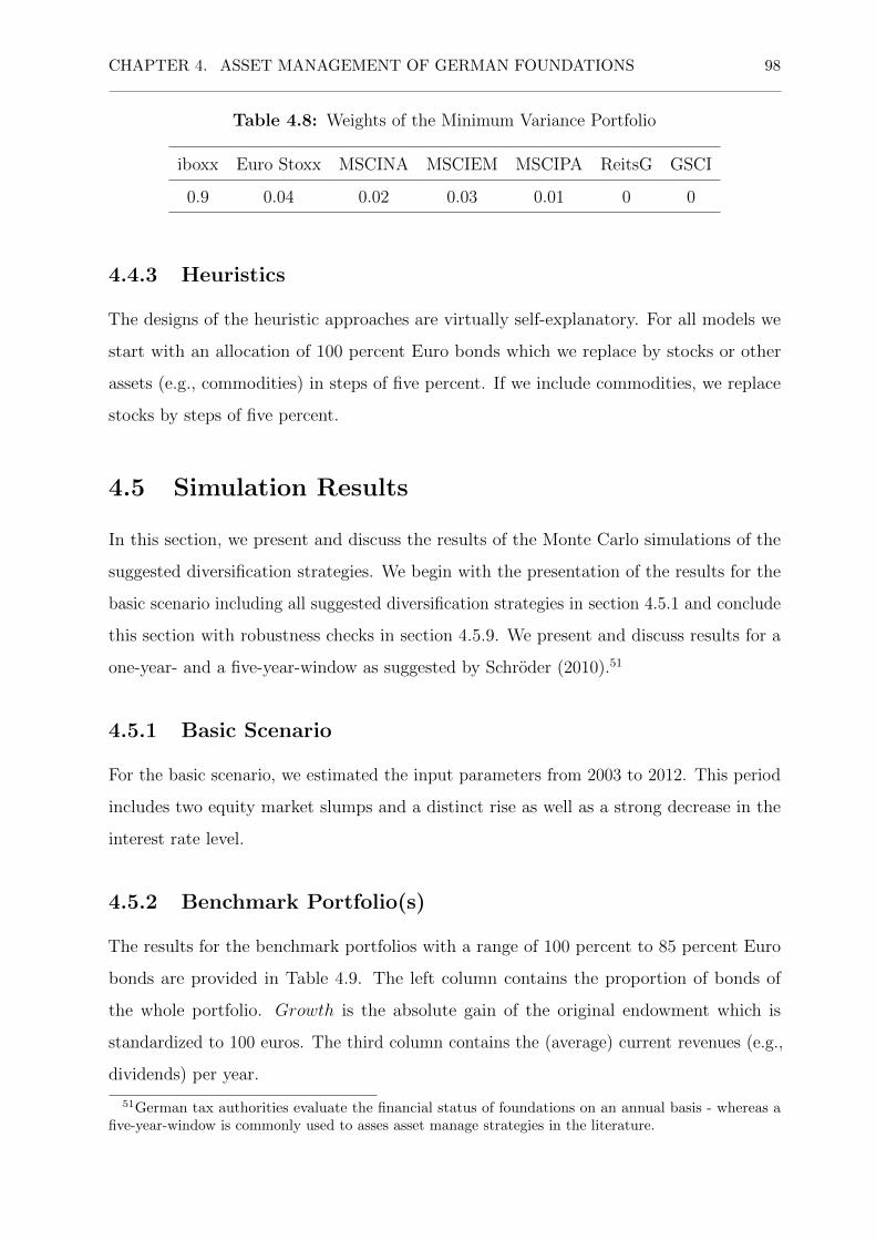
CHAPTER 4. ASSET MANAGEMENT OF GERMAN FOUNDATIONS 98
Table 4.8: Weights of the Minimum Variance Portfolio
iboxx Euro Stoxx MSCINA MSCIEM MSCIPA ReitsG GSCI
0.9 0.04 0.02 0.03 0.01 0 0
4.4.3 Heuristics
The designs of the heuristic approaches are virtually self-explanatory. For all models we
start with an allocation of 100 percent Euro bonds which we replace by stocks or other
assets (e.g., commodities) in steps of five percent. If we include commodities, we replace
stocks by steps of five percent.
4.5 Simulation Results
In this section, we present and discuss the results of the Monte Carlo simulations of the
suggested diversification strategies. We begin with the presentation of the results for the
basic scenario including all suggested diversification strategies in section 4.5.1 and conclude
this section with robustness checks in section 4.5.9. We present and discuss results for a
one-year- and a five-year-window as suggested by Schroder (2010).51
4.5.1 Basic Scenario
For the basic scenario, we estimated the input parameters from 2003 to 2012. This period
includes two equity market slumps and a distinct rise as well as a strong decrease in the
interest rate level.
4.5.2 Benchmark Portfolio(s)
The results for the benchmark portfolios with a range of 100 percent to 85 percent Euro
bonds are provided in Table 4.9. The left column contains the proportion of bonds of
the whole portfolio. Growth is the absolute gain of the original endowment which is
standardized to 100 euros. The third column contains the (average) current revenues (e.g.,
dividends) per year.
51German tax authorities evaluate the financial status of foundations on an annual basis - whereas afive-year-window is commonly used to asses asset manage strategies in the literature.
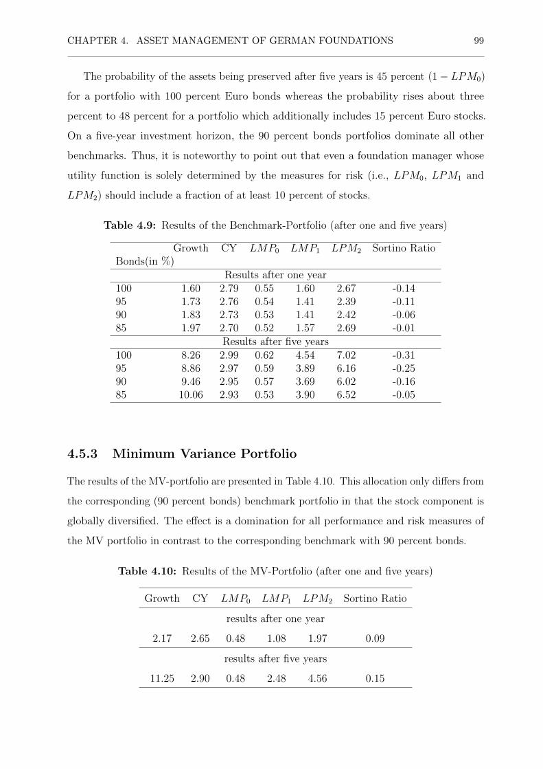
CHAPTER 4. ASSET MANAGEMENT OF GERMAN FOUNDATIONS 99
The probability of the assets being preserved after five years is 45 percent (1− LPM0)
for a portfolio with 100 percent Euro bonds whereas the probability rises about three
percent to 48 percent for a portfolio which additionally includes 15 percent Euro stocks.
On a five-year investment horizon, the 90 percent bonds portfolios dominate all other
benchmarks. Thus, it is noteworthy to point out that even a foundation manager whose
utility function is solely determined by the measures for risk (i.e., LPM0, LPM1 and
LPM2) should include a fraction of at least 10 percent of stocks.
Table 4.9: Results of the Benchmark-Portfolio (after one and five years)
Growth CY LMP0 LMP1 LPM2 Sortino RatioBonds(in %)
Results after one year100 1.60 2.79 0.55 1.60 2.67 -0.1495 1.73 2.76 0.54 1.41 2.39 -0.1190 1.83 2.73 0.53 1.41 2.42 -0.0685 1.97 2.70 0.52 1.57 2.69 -0.01
Results after five years100 8.26 2.99 0.62 4.54 7.02 -0.3195 8.86 2.97 0.59 3.89 6.16 -0.2590 9.46 2.95 0.57 3.69 6.02 -0.1685 10.06 2.93 0.53 3.90 6.52 -0.05
4.5.3 Minimum Variance Portfolio
The results of the MV-portfolio are presented in Table 4.10. This allocation only differs from
the corresponding (90 percent bonds) benchmark portfolio in that the stock component is
globally diversified. The effect is a domination for all performance and risk measures of
the MV portfolio in contrast to the corresponding benchmark with 90 percent bonds.
Table 4.10: Results of the MV-Portfolio (after one and five years)
Growth CY LMP0 LMP1 LPM2 Sortino Ratio
results after one year
2.17 2.65 0.48 1.08 1.97 0.09
results after five years
11.25 2.90 0.48 2.48 4.56 0.15

CHAPTER 4. ASSET MANAGEMENT OF GERMAN FOUNDATIONS 100
4.5.4 Heuristics - Euro Investments
Figure 4.7 provides the results for exclusive Euro-portfolios for a five-year investment
horizon and it illustrates the trade-off between risk and performance measures.52 These
allocations include Euro bonds which are represented by the iboxx Euro Overall as suggested
by Jacobs et al. (2014) and stocks which are represented by the Euro Stoxx. We start with
an allocation of 100 percent bonds which we replace by stocks in steps of five percent.
The probability for a preservation of assets in real terms measured by 1− LMP0 varies
between 39 percent for an equity ratio of zero percent and 50 percent for ratios between
35 and 65 percent. The main result of these simulations is that a foundation manager
who wants to maintain her assets in reals terms would hold at least 10 percent stocks and
probably not more than 20 percent. Thus, for exclusive Euro-investments the benchmark
portfolios can be an efficient allocation.
4.5.5 Heuristics - GDP-Weighted Stocks
The effect of a global diversification of the stock component with GDP-weighted region-
specific indices as suggested by Jacobs et al. (2014) is provided in Figure 4.8 and Table 4.12.
The probability for the preservation of assets is highest (69 percent53) for equity ratios of
50 to 70 percent.
4.5.6 Heuristics - Equally-Weighted Stocks
The results for the portfolios with a 1N
-weighted stock component are slightly inferior to
the GDP-weighted heuristic. These findings provided in Table 4.13 are in line with the
simulation results of Jacobs et al. (2014). Nevertheless, Figure 4.9 illustrates that this
heuristic exhibits the same pattern as the GDP-approach. Adding worldwide diversified
(i.e., GDP- or 1N
-weighted) stocks to a 100 percent Euro bond portfolio leads to a decrease
of LPM0 up to an allocation of 70 percent bonds and 30 percent stocks. From this level
on, (potential) additional growth of the foundations assets are accompanied by an increase
in the downside risk measures.
52From this point we provide the long-term (5 years) results.53This implies a LPM0 = 0.3136.

CHAPTER 4. ASSET MANAGEMENT OF GERMAN FOUNDATIONS 101
Figure 4.7: Results Euro-Investments (five years)
020
4060
8010
0
0 5 10 15 20
Gro
wth
0 1 2 3 4
Rev
enue
0 0.10.20.30.40.50.6
LPM
0
0 5 10 15
LPM
1
0 5 10 15 20 25 30
LPM
2_SD
−0.3−0.2−0.10 0.10.20.3
Sorti
no
Table 4.11: Results Euro Investments (five years)
Growth CY LMP0 LMP1 LPM2 Sortino RatioBonds (in %)100 8.32 2.98 0.61 4.52 7.01 -0.3095 8.86 2.97 0.59 3.88 6.16 -0.2590 9.46 2.96 0.57 3.69 6.02 -0.1585 10.07 2.93 0.54 3.90 6.52 -0.0580 10.67 2.91 0.52 4.38 7.42 0.0475 11.28 2.89 0.51 5.02 8.56 0.1070 11.89 2.87 0.51 5.74 9.83 0.1565 12.50 2.84 0.50 6.53 11.18 0.1960 13.11 2.83 0.50 7.35 12.55 0.2155 13.73 2.80 0.50 8.19 13.96 0.2450 14.35 2.78 0.50 9.05 15.37 0.2645 14.98 2.76 0.50 9.92 16.78 0.2740 15.59 2.73 0.50 10.81 18.19 0.2935 16.21 2.70 0.50 11.70 19.59 0.3030 16.84 2.69 0.51 12.60 20.99 0.3125 17.47 2.66 0.51 13.51 22.37 0.3220 18.10 2.63 0.51 14.42 23.75 0.3215 18.73 2.61 0.51 15.34 25.12 0.3310 19.36 2.59 0.52 16.27 26.47 0.345 20.00 2.56 0.52 17.19 27.82 0.340 20.63 2.53 0.53 18.13 29.16 0.35

CHAPTER 4. ASSET MANAGEMENT OF GERMAN FOUNDATIONS 102
Figure 4.8: Results GDP-Weighted Stocks Components (five years)
020
4060
8010
0
0 10 20 30 40
Gro
wth
0 2 4 6 8
Rev
enue
0 0.1 0.2 0.3 0.4 0.5 0.6LP
M0
0 2 4 6
LPM
1
0 5 10 15
LPM
2_SD
0 0.5 1 1.5
Sorti
no
Table 4.12: Results GDP-Weighted Stock Components (five years)
Growth CY LMP0 LMP1 LPM2 Sortino RatioBonds (in %)100 8.32 2.98 0.61 4.52 7.01 -0.3095 9.72 2.96 0.55 3.43 5.68 -0.1290 11.33 2.93 0.48 2.69 4.84 0.1485 12.56 2.90 0.41 2.30 4.60 0.4880 14.00 2.87 0.37 2.19 4.54 0.7975 15.46 2.84 0.35 2.26 4.85 1.0470 16.93 2.80 0.33 2.43 5.32 1.2265 18.42 2.77 0.32 2.67 5.90 1.3660 19.92 2.74 0.32 2.95 6.55 1.4555 21.44 2.70 0.32 3.25 7.25 1.5250 22.98 2.67 0.31 3.58 7.98 1.5845 24.53 2.63 0.31 3.93 8.72 1.6240 26.09 2.59 0.31 4.28 9.48 1.6535 27.68 2.55 0.31 4.65 10.25 1.6830 29.28 2.51 0.31 5.03 11.03 1.7125 30.89 2.47 0.32 5.41 11.81 1.7320 32.52 2.43 0.32 5.80 12.60 1.7615 34.17 2.38 0.32 6.20 13.38 1.7810 35.82 2.34 0.32 6.61 14.18 1.795 37.52 2.29 0.33 7.02 14.96 1.810 39.32 2.24 0.33 7.43 15.76 1.82

CHAPTER 4. ASSET MANAGEMENT OF GERMAN FOUNDATIONS 103
Figure 4.9: Results 1N
-Weighted Stocks Components (five years)
020
4060
8010
0
0 10 20 30
Gro
wth
0 2 4 6
Rev
enue
0 0.1 0.2 0.3 0.4 0.5 0.6
LPM
0
0 2 4 6
LPM
1
0 5 10 15
LPM
2_SD
0 0.5 1 1.5
Sorti
no
Table 4.13: Results 1N
-Weighted Stock Components (five years)
Growth CY LMP0 LMP1 LPM2 Sortino RatioBonds (in %)100 8.32 2.98 0.61 4.52 7.01 -0.3095 9.59 2.96 0.55 3.51 5.78 -0.1490 10.88 2.92 0.49 2.81 5.00 0.0985 12.17 2.89 0.43 2.45 4.67 0.3780 13.48 2.86 0.39 2.34 4.71 0.6575 14.81 2.82 0.37 2.40 5.01 0.8870 16.13 2.79 0.35 2.57 5.46 1.0565 17.48 2.75 0.34 2.80 6.01 1.1760 18.84 2.72 0.33 3.08 6.67 1.2755 20.22 2.68 0.33 3.39 7.35 1.3350 21.61 2.64 0.33 3.71 8.07 1.3945 23.01 2.60 0.33 4.06 8.81 1.4340 24.43 2.56 0.33 4.42 9.56 1.4635 25.84 2.52 0.33 4.79 10.31 1.4930 27.28 2.48 0.33 5.16 11.09 1.5225 28.74 2.43 0.33 5.55 11.86 1.5520 30.22 2.39 0.34 5.94 12.64 1.5615 31.68 2.35 0.34 6.35 13.42 1.5810 33.18 2.30 0.34 6.79 14.21 1.615 34.69 2.25 0.34 7.17 14.99 1.620 36.21 2.20 0.34 7.59 15.78 1.63

CHAPTER 4. ASSET MANAGEMENT OF GERMAN FOUNDATIONS 104
4.5.7 Commodities
Table 4.14 summarizes the simulation results for different commodity ratios: 5, 10, and 15
percent.54 For reasons of clarity, we provide the results for all three ratios in steps of 10
percent. We can find the following effects: the inclusion of commodities into a foundation’s
portfolio can lead to decreasing returns, increasing volatility and decreasing current yields.
Thus, based on these results, commodities cannot add value to the asset management of
German foundations.
Table 4.14: Results GDP-Weighted Stocks and Commodities (five years)
Growth CY LMP0 LMP1 LPM2 Sortino RatioBonds (in %)
5 Percent Commodities90 10.22 2.82 0.52 3.21 5.49 -0.0380 13.04 2.76 0.40 3.21 5.65 0.5770 16.16 2.70 0.34 2.42 5.35 1.0460 19.47 2.73 0.33 2.55 6.49 1.3650 22.34 2.56 0.32 2.96 7.85 1.5240 25.58 2.48 0.32 3.56 9.33 1.6330 28.83 2.38 0.32 4.45 10.85 1.6920 32.48 2.31 0.33 4.96 12.43 1.7310 35.46 2.22 0.33 5.72 13.93 1.85
10 Percent Commodities90 9.22 2.71 0.57 4.31 6.86 -0.1780 12.23 2.65 0.45 3.51 5.91 0.3870 15.13 2.58 0.38 2.96 5.99 0.8260 18.18 2.51 0.35 3.12 6.78 1.1450 21.11 2.43 0.33 3.71 8.01 1.3540 24.48 2.36 0.32 4.33 9.40 1.4930 27.73 2.27 0.32 5.02 10.87 1.5920 31.06 2.18 0.33 5.75 12.45 1.6710 34.45 2.09 0.33 6.51 13.92 1.72
15 Percent Commodities90 9.22 2.71 0.57 4.31 6.86 -0.1780 11.14 2.53 0.50 4.05 7.04 0.1070 14.10 2.47 0.41 3.54 6.97 0.5460 17.13 2.39 0.37 3.63 7.40 0.9150 20.23 2.32 0.35 4.01 8.44 1.1640 23.39 2.24 0.34 4.56 9.70 1.3330 26.62 2.15 0.33 5.20 11.08 1.4620 29.92 2.06 0.33 5.88 12.53 1.5510 33.29 1.97 0.33 6.62 14.01 1.63
5415 percent is the proportion Jacobs et al. (2014) recommend for private investors.

CHAPTER 4. ASSET MANAGEMENT OF GERMAN FOUNDATIONS 105
4.5.8 Welfare Losses
In this section, we summarize the results for the basic scenario in order to analyze whether
the empirical investment behavior of German foundations can lead to welfare losses.
Since the funds of a foundation have to be used for purposes of public interest, welfare
losses occur with regard to a specific asset allocation if there is another allocation which
has the same or lower risk but can provide higher returns at the same time.
The GDP-heuristic dominates the Euro investments, including the benchmark portfolios,
for every corresponding allocation with regard to all performance and risk measures.
For these reasons, we define a risk equivalent (RE) that is represented by the globally
diversified portfolio RE (Global) which provides the same or less risk with regard to all
downside risk measures (LM0, LM1, LM2) as the corresponding Euro portfolio.
According to the utility function of the foundation manager, we have localized welfare
losses due to two possible kinds of individual choice behavior. A foundation manager whose
focus is on the downside volatility (LPM2) would choose the 90 percent bond portfolio in
the case of exclusive Euro investments and she would choose the 80 percent bond portfolio
in the case of a globally diversified and GDP-weighted stock component. A foundation
manager who uses the probability for a preservation of assets (LPM0) as selection criteria
to solve the trade-off between risk and performance measures would choose not more than
35 percent stocks in the case of mere Euro investments and not more than 50 percent
stocks in the case of the GDP-heuristic. Table 4.15 summarizes the effects of this choice
behavior.
Given both potential choice behaviors, the welfare loss is determined by the difference
between the absolute growth of the Euro portfolio and the growth of the globally diversified
portfolio (lower boundary) and the RE (upper boundary). As Table 4.15 shows, the welfare
loss for a foundation manager with a focus on the preservation of assets is twice as high as
for a manager who wants to minimize downside risks. Table 4.15 illustrates and quantifies
the external effects (i.e., welfare losses) of a regulatory framework that provides incentives
for risk avoidance.
Empirical asset allocations (e.g., 90 percent Euro bonds portfolios) can generate welfare
losses from 40 to 90 percent55 of their (actual) returns due to asset management strategies
with a focus on exaggerated risk avoidance.
55In addition, it must be considered that the average revenue of the representative benchmark portfolio

CHAPTER 4. ASSET MANAGEMENT OF GERMAN FOUNDATIONS 106
Table 4.15: Choice Behavior and Welfare Losses
Bonds Growth CY LMP0 LMP1 LPM2 Sortino RatioFocus on Downside Volatility (LPM2)
Euro 90 9.46 2.96 0.57 3.69 6.02 -0.15Global 80 14.00 2.87 0.37 2.19 4.54 0.79RE(Global) 65 18.42 2.77 0.32 2.67 5.90 1.36Welfare loss [4.54, 8.96]
Focus on Preservation of Assets (LPM0)Euro 65 12.50 2.84 0.50 6.53 11.18 0.19Global 50 22.98 2.67 0.31 3.58 7.98 1.58RE(Global) 30 29.28 2.51 0.31 5.03 11.03 1.71Welfare loss [10.48, 16.78]
Potential welfare losses (LPM2): 4.54 = 14− 9.46, 8.96 = 18.42− 9.46; (LPM0): 10.48 =22.98− 12.50, 16.78 = 29.28− 12.50
In summary, Table 4.15 shows that, given the risks German foundations actually take
(on average), there is a huge welfare loss due to biased perception of these risks. The
following example illustrates this problem: a German foundation is founded with an
endowment of 1 million euros. Given the empirical allocation of 90 percent Euro bonds and
10 percent Euro stocks, this foundation would exhibit an absolute growth of 94,600 euros
after five years whereas an allocation which provides the same (or lower) risk measures due
to a globally diversified stock portfolio would lead to an absolute growth of 184,200 euros.
If we assume a spending rate of three percent per year, this choice behavior would lead
to a loss in a foundation’s expenditures for charitable purposes of approx. 5,500 euros for
year five. With respect to the small and mid-sized German foundations that we focus on
with assets under management of nearly 70 billion euros, this loss would amount to nearly
385 million euros.
is slightly higher than the revenues of efficient allocations.

CHAPTER 4. ASSET MANAGEMENT OF GERMAN FOUNDATIONS 107
4.5.9 Results - Subscenarios
In this section, we provide the results of the robustness checks for the five year horizon. We
run Monte Carlo simulations for two subscenarios: a period (i.e., subscenario) with a rise in
the level of interest rates and a subscenario with a decrease in interest rates. In section 4.5.1,
we have shown that foundation managers who do not only aim at growing their assets
should invest a large proportion of their funds in bonds. Thus, both subscenarios can be
seen as a check for (worst-case) robustness.
Benchmark Portfolio(s)
The simulation results for both subscenarios, provided in Table 4.16, are nearly inverse. For
the first subscenario, a period with a persistently rising interest rate level, the probability
for the assets of being preserved is virtually zero for the first three benchmark portfolios.56
By contrast, the portfolios with 100 percent or 95 percent Euro bonds would have preserved
the original funds with probability of 100 percent for the second subscenario, a period with
a rapidly decreasing interest rate level.
Table 4.16: Results of the Benchmark-Portfolio (after five years)
Growth CY LMP0 LMP1 LPM2 Sortino RatioBonds(in %)
2003 - 2007100 -14.41 2.50 1.00 24.81 25.38 -0.9895 -9.92 2.55 1.00 20.33 20.98 -0.9790 -5.25 2.61 0.99 15.66 16.64 -0.9485 -0.38 2.66 0.94 10.97 12.66 -0.85
2008 - 2012100 28.73 3.36 0.03 0.12 0.87 21.0195 25.03 3.27 0.05 0.19 1.07 13.6990 21.42 3.19 0.14 0.61 2.14 5.1485 17.89 3.11 0.29 1.87 4.37 1.71
56There is anecdotal evidence that some German foundations put their funds into long-term bonds(e.g.,15 or 20 years) in order to generate current income over the recent past. Such a duration wouldstrengthen the effect of rising interest rates.

CHAPTER 4. ASSET MANAGEMENT OF GERMAN FOUNDATIONS 108
Minimum Variance Portfolio
The results of the MV-portfolio for both subscenarios are provided in Table 4.17. Since
the allocation of the MV-Portfolio is quite similar to the benchmark portfolio with 90
percent Euro bonds, the results resemble each other. Nevertheless, with regard to all risk
and performance measures the MV-portfolio seems to exhibit a slightly higher worst-case
robustness with regard to all performance and risk measures than the corresponding
benchmark portfolio due to a diversified stock component.
Table 4.17: Results of the MV-Portfolio (after five years)
Assets CY LMP0 LMP1 LPM2 Sortino Ratio2003 - 2007
95.65 2.63 0.97 14.99 15.89 -0.912008 - 2012
123.39 3.21 0.11 0.59 2.24 5.32

CHAPTER 4. ASSET MANAGEMENT OF GERMAN FOUNDATIONS 109
Euro Investments and GDP-Weighted Stocks
Table 4.19 and Table 4.18 provide the results for the subscenarios of exclusive Euro-
Investments and portfolios with GDP-weighted stocks.
A focus on the downside variance LPM2 would lead to extreme allocations: 100 percent
stocks for 2003 - 2007 and 95 to 100 percent bonds for 2008 - 2012. Whereas, a focus
on the LPM0 would lead to an allocation of 80 percent bonds and 20 percent globally
diversified stocks for both scenarios.

CHAPTER 4. ASSET MANAGEMENT OF GERMAN FOUNDATIONS 110
Table 4.18: Results of Euro-Investments (after five years)
Growth CY LMP0 LMP1 LPM2 Sortino RatioBonds(in %)
2003 - 2007100 -14.41 2.50 1.00 24.81 25.38 -0.9895 -9.92 2.55 1.00 20.33 20.98 -0.9790 -5.25 2.61 0.99 15.66 16.64 -0.9485 -0.38 2.66 0.94 10.97 12.66 -0.8580 4.69 2.71 0.76 6.99 9.42 0.6175 9.96 2.76 0.55 4.27 7.10 -0.0670 15.44 2.81 0.36 2.66 5.55 0.9165 21.13 2.85 0.24 1.75 4.52 2.3760 27.05 2.90 0.17 1.22 3.83 4.3455 33.20 2.94 0.12 0.90 3.37 6.7650 39.58 2.98 0.09 0.71 3.05 9.5645 46.21 3.02 0.07 0.58 2.83 12.6740 53.09 3.05 0.06 0.49 2.66 16.0435 60.22 3.09 0.05 0.43 2.54 19.6030 67.62 3.12 0.04 0.38 2.46 23.3025 75.29 3.14 0.04 0.35 2.39 27.1020 83.24 3.17 0.03 0.32 2.35 30.9515 91.47 3.19 0.03 0.30 2.33 34.8310 100.00 3.20 0.03 0.28 2.31 38.735 108.82 3.22 0.02 0.27 2.31 42.620 117.96 3.22 0.02 0.26 2.31 46.50
2008 - 2012100 28.73 3.36 0.03 0.12 0.87 21.0195 25.03 3.27 0.05 0.19 1.07 13.6990 21.42 3.19 0.14 0.61 2.14 5.1485 17.89 3.11 0.29 1.87 4.37 1.7180 14.43 3.03 0.43 4.03 7.53 0.5375 11.07 2.96 0.54 6.82 11.20 0.0670 7.78 2.89 0.61 9.90 15.02 -0.1765 4.57 2.81 0.65 13.09 18.94 -0.3160 1.44 2.74 0.69 16.32 22.77 -0.3955 -1.61 2.67 0.71 19.51 26.52 -0.4550 -4.59 2.60 0.73 22.68 30.16 -0.5045 -7.50 2.53 0.75 25.80 33.69 -0.5340 -10.34 2.46 0.77 28.86 37.10 -0.5635 -13.11 2.40 0.78 31.84 40.39 -0.5830 -15.80 2.34 0.79 34.79 43.57 -0.6020 -18.43 2.27 0.80 37.66 46.65 -0.6115 - 21.00 2.21 0.81 40.46 49.60 -0.6310 -23.50 2.16 0.82 43.20 52.45 -0.655 -28.30 2.04 0.83 48.46 57.85 -0.670 -30.61 1.99 0.84 51.00 60.41 -0.68
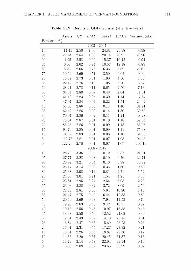
CHAPTER 4. ASSET MANAGEMENT OF GERMAN FOUNDATIONS 111
Table 4.19: Results of GDP-heuristic (after five years)
Assets CY LMP0 LMP1 LPM2 Sortino RatioBonds(in %)
2003 - 2007100 -14.41 2.50 1.00 24.81 25.38 -0.9895 -9.73 2.54 1.00 20.14 20.91 -0.9690 -4.95 2.58 0.99 15.37 16.42 -0.9485 0.03 2.62 0.94 10.57 12.18 -0.8580 5.23 2.66 0.76 6.36 8.62 -0.6175 10.64 2.69 0.51 3.50 6.02 0.0470 16.27 2.73 0.31 1.90 4.30 1.3665 22.12 2.76 0.19 1.08 3.20 3.6760 28.21 2.78 0.11 0.65 2.50 7.1355 34.54 2.80 0.07 0.43 2.04 11.8150 41.13 2.83 0.05 0.30 1.74 17.6445 47.97 2.84 0.04 0.22 1.54 24.4240 55.05 2.86 0.03 0.17 1.40 31.9135 62.42 2.86 0.02 0.14 1.30 39.8930 70.07 2.86 0.02 0.11 1.24 48.2825 78.01 2.87 0.01 0.10 1.18 57.0420 86.23 2.86 0.01 0.09 1.15 66.0815 94.76 2.85 0.01 0.09 1.11 75.3810 105.60 2.83 0.01 0.08 1.10 84.865 112.75 2.81 0.01 0.07 1.08 94.460 122.23 2.78 0.01 0.07 1.07 104.13
2008 - 2012100 28.73 3.36 0.03 0.12 0.87 21.0195 27.77 3.28 0.03 0.10 0.76 22.7190 26.97 3.21 0.04 0.16 0.98 16.8285 26.17 3.14 0.08 0.35 1.60 9.8380 25.38 3.08 0.14 0.81 2.71 5.5275 24.60 3.01 0.21 1.54 4.25 3.3370 23.81 2.95 0.27 2.54 6.08 2.2065 23.03 2.88 0.32 3.72 8.09 2.5660 22.25 2.81 0.36 5.04 10.20 1.1655 21.47 2.75 0.40 6.44 12.35 0.8950 20.69 2.69 0.43 7.94 14.53 0.7045 19.93 2.63 0.46 9.42 16.71 0.5740 19.15 2.56 0.48 10.97 18.88 0.4635 18.38 2.50 0.50 12.52 21.02 0.3930 17.61 2.43 0.52 14.10 23.15 0.3125 16.84 2.47 0.53 15.69 25.25 0.2520 16.01 2.31 0.55 17.27 27.32 0.2115 15.31 2.26 0.56 18.87 29.36 0.1710 14.55 2.20 0.57 20.45 31.37 0.135 13.79 2.14 0.58 22.04 33.34 0.100 13.03 2.08 0.59 23.63 35.29 0.07

CHAPTER 4. ASSET MANAGEMENT OF GERMAN FOUNDATIONS 112
Welfare Loss - Scenarios
In summary, Table 4.20 provides the calculated welfare losses for both subscenarios. In
comparison with the results of the basic period (Table 4.15), a foundation manager with a
focus on downside volatility would prefer extreme allocations (i.e., 0 or 95 to 100 percent
Euro bonds). A manager who prefers the preservation of assets would choose 80 to 90
percent Euro bonds. This behavior is due to the outperformance of stocks in 2003 - 2007 (in
relation to bonds) and the outperformance of bonds in 2008 - 2012 (in relation to stocks).
However, welfare losses due to an inefficiently diversified stock component are lower than
for the basic scenario but still occur (except for a downside-volatility-averse manager in the
second subscenario (2008-2012)). We can show that even for extreme scenarios a higher
and GDP-weighted stock component can provide additional utility and reduce welfare
losses caused by exclusive Euro-investments.
Table 4.20: Choice Behavior and Welfare Losses
Bonds Growth CY LMP0 LMP1 LPM2 Sortino RatioFocus on Downside Volatility (LPM2)
2003 - 2007Euro 0 117.96 3.22 0.02 0.26 2.31 46.50Global 0 122.23 2.78 0.01 0.07 1.07 104.13RE(Global) 0 122.23 2.78 0.01 0.07 1.07 104.13Welfare loss 4.27
2008 - 2012Euro 100 28.73 3.36 0.03 0.12 0.87 21.01Global 95 27.77 3.28 0.03 0.10 0.76 22.71RE(Global) 100 28.73 3.36 0.03 0.12 0.87 21.01Welfare loss -
Focus on Preservation of Assets (LPM0)2003 - 2007
Euro 90 9.46 2.96 0.57 3.69 6.02 -0.15Global 80 14.00 2.87 0.37 2.19 4.54 0.79RE(Global) 65 18.42 2.77 0.32 2.67 5.90 1.36Welfare loss [4.54, 8.96]
2008 - 2012Euro 90 9.46 2.96 0.57 3.69 6.02 -0.15Global 80 14.00 2.87 0.37 2.19 4.54 0.79RE(Global) 65 18.42 2.77 0.32 2.67 5.90 1.36Welfare loss [4.54, 8.96]
CHAPTER 4. ASSET MANAGEMENT OF GERMAN FOUNDATIONS 113
4.6 Conclusion
Our study has two objectives. First of all, we define a legal and financial framework for the
asset management of German foundations in order to derive efficient asset management
strategies within this framework. Based on a summary of the legal literature and current
jurisprudence we can show that asset managers of German foundations cannot be held
liable for losses if they had sufficiently diversified the respective foundation’s assets before.
We therefore compare different approaches and test their suitability for the purposes of
German non-profit foundations by means of stochastic simulations. We find that foundation
portfolios should at least consist of bonds and globally diversified stocks. With regard to
the weights of the stocks we find evidence that a (worldwide) GPD-weighting as suggested
by Jacobs et al. (2014) provides superior results compared to exclusive Euro investments
or even worldwide equally weighted stocks.
Second, we can show that the empirical investment behavior of German foundations with
a focus on Euro investments leads to welfare losses. Given the objectives of a foundation
manager, these losses arise if a chosen asset allocation is dominated by another allocation
which provides a higher return for the same (or even lower) risk measures at the same
time. For stochastically simulated asset markets, we show that this can be the case
for a portfolio with a globally diversified stock component in contrast to exclusive Euro
investments. By comparing the empirical investment behavior of German foundations
with our stochastically simulated results we can quantify these welfare losses. Small and
mid-sized German foundations which altogether manage assets of 70 billion euros could
provide up to 77 million euros of additional spending for charitable purposes per year if
they were to hold a higher (i.e., ten percent) worldwide diversified stock component. Such
a portfolio would provide the same or even lower risk measures.
This problem could be caused by a biased understanding of risk and a focus on short-
term volatility risk measures instead. Therefore, we suggest the implementation regulatory
incentives such as the five percent rule in the USA. A foundation which has to spend a
certain amount (e.g., five percent) of its endowment per year could be nudged to take risks
in a more efficient way than a foundation whose manager can only be held liable for losses.
Furthermore, such a rule would provide a clear regulatory framework with less room
for interpretation and regulatory arbitrage, as suggested by Admati and Hellwig (2014) for
the banking industry.

CHAPTER 4. ASSET MANAGEMENT OF GERMAN FOUNDATIONS 114
References
Admati, Anat and Martin Hellwig (2014). The Bankers’ New Clothes: What’s Wrong with
Banking and What to Do About It. Princeton University Press.
Allen, Gregory (2010). “The Risk Parity Approach to Asset Allocation”. Callan Investments
Institute.
Annaert, Jan, Sofieke Van Osselaer, and Bert Verstraete (2009). “Performance Evaluation
of Portfolio Insurance Strategies Using Stochastic Dominance Criteria”. Journal of
Banking & Finance 33(2), 272–280.
Bajeux-Besnainou, Isabelle and Kurtay Ogunc (2006). “Spending Rules for Endowment
Funds”. Review of Quantitative Finance and Accounting 27(1), 93–107.
Benninga, Simon and Marshall Blume (1985). “On the Optimality of Portfolio Insurance”.
Journal of Finance 40(5), 1341–1352.
Black, Fischer and Robert C. Jones (1987). “Simplifying Portfolio Insurance”. Journal of
Portfolio Management 14(1), 48–51.
Black, Fischer and Andre F Perold (1992). “Theory of Constant Proportion Portfolio
Insurance”. Journal of Economic Dynamics and Control 16(3-4), 403–426.
Black, Fischer and Myron Scholes (1973). “The Pricing of Options and Corporate Liabilities”.
Journal of Political Economy, 637–654.
Boeckler, Hans Stiftung (2013). WSI-Tarifarchiv Stand 31.12.2013. Dusseldorf.
Bundesverband Deutscher Stiftungen (2010). StiftungsReport 2010/11. Verlag des Bun-
desverbandes Deutscher Stiftungen.
Bundesverband Deutscher Stiftungen (2014a). Gewichtete Verteilung der Stiftungszwecke.
Bundesverband Deutscher Stiftungen (2014b). Stiftungen in Zahlen 2013.
Bundesverband Deutscher Stiftungen (2014c). Stiftungen und Vermogen in Klassen.
Bundesverband Deutscher Stiftungen (2015). “Stiftungen in den Bundeslandern im Uberblick”.
Carstensen, Carsten (1996). “Die ungeschmalerte Erhaltung des Stiftungsvermogens”. Die
Wirtschaftsprufung 49, 781–793.

CHAPTER 4. ASSET MANAGEMENT OF GERMAN FOUNDATIONS 115
Carstensen, Carsten (2003). “Vermogensverwaltung”. In: Handbuch Stiftungen. Springer,
535–563.
Choie, Kenneth S” Nicholas” and Eric J Seff (1989). “TIPP: Insurance without Complexity:
Comment”. Journal of Portfolio Management 16(1), 107–108.
DeMiguel, Victor, Lorenzo Garlappi, and Raman Uppal (2009). “Optimal Versus Naive
Diversification: How Inefficient Is the 1/N Portfolio Strategy?” Review of Financial
Studies 22(5), 1915–1953.
Detemple, Jerome B, Rene Garcia, and Marcel Rindisbacher (2003). “A Monte Carlo
Method for Optimal Portfolios”. Journal of Finance 58(1), 401–446.
Dichtl, Hubert and Wolfgang Drobetz (2011). “Portfolio Insurance and Prospect Theory
Investors: Popularity and Optimal Design of Capital Protected Financial Products”.
Journal of Banking & Finance 35(7), 1683–1697.
Dichtl Hubert and, Wolfgang and Martin Wambach (2014). “Where is the Value Added
of Rebalancing? A Systematic Comparison of Alternative Rebalancing Strategies”.
Financial Markets and Portfolio Management 28(3), 209–231.
Dimmock, Stephen G (2012). “Background Risk and University Endowment Eunds”. Review
of Economics and Statistics 94(3), 789–799.
Duchin, Ran and Haim Levy (2009). “Markowitz Versus the Talmudic Portfolio Diversifica-
tion Strategies”. Journal of Portfolio Management 35(2), 71–74.
Dybvig, Philip H (1999). “Using Asset Allocation to Protect Spending”. Financial Analysts
Journal, 49–62.
Estep, Tony and Mark Kritzman (1988). “TIPP: Insurance without Complexity”. Journal
of Portfolio Management 14(4), 38–42.
Falk, Hermann (2011). Vermogensanlage - Stiftungsvermogen professionell Verwalten - ein
Leitfaden. Bundesverband Deutscher Stiftungen.
Fecht, Falko and Michael Wedow (2014). “The Dark and the Bright Side of Liquidity
Risks: Evidence from Open-End Real Estate Funds in Germany”. Journal of Financial
Intermediation 23(3), 376–399.

CHAPTER 4. ASSET MANAGEMENT OF GERMAN FOUNDATIONS 116
Fishburn, P.C. (1977). “Mean-Risk Analysis with Risk Associated with Below-Target
Returns”. American Economic Review, 116–126.
Haake, Stefan R. (2013). Stiftungsfonds: Antwort auf die Ertragsfalle? – Quantitative und
qualitative Analyse von in Deutschland zugelassenen Stiftungsfonds sowie Empfehlungen
fur die Praxis der Kapitalanlage von Stiftungen. Frankfurt.
Harvey, Campbell R, Yan Liu, and Heqing Zhu (2015). “... And the Cross-Section of
Expected Returns”. Review of Financial Studies 29, 5–68.
Heissmann (2004). Planung, Anlage und Kontrolle von Stiftungsvermogen bei Deutschen
Stiftungen, Heissmann. Wiesbaden.
Heissmann (2005). Planung, Anlage und Kontrolle von Stiftungsvermogen bei Deutschen
Stiftungen, Heissmann. Wiesbaden.
Hull, John (2011). Options, Futures and other Derivatives. Pearson Education.
Huttemann, Rainer (2014). Gemeinnutzigkeits- und Spendenrecht. Otto Schmidt.
Huttemann, Rainer and Wolfgang Schon (2007). Vermogensverwaltung und Vermogenser-
haltung im Stiftungs-und Gemeinnutzigkeitsrecht. Heymann.
Ioannidis, John PA (2005). “Why Most Published Research Findings Are False”. PLoS
Medicine 2(8), e124.
Jacobs, Heiko, Sebastian Muller, and Martin Weber (2014). “How Should Individual
Investors Diversify? An Empirical Evaluation of Alternative Asset Allocation Policies”.
Journal of Financial Markets 19, 62–85.
Kritzman, Mark, Sebastien Page, and David Turkington (2010). “In Defense of Optimization:
The Fallacy of 1/N”. Financial Analysts Journal 66(2), 31–39.
Lee, Wai (2011). “Risk-Based Asset Allocation: A New Answer to an Old Question?”
Journal of Portfolio Management 37(4), 11.
Lerven, Frank van (2016). “Quantitative Easing in the Eurozone: a One-Year Assessment”.
Intereconomics 51(4), 237–242.
Merton, Robert C (1993). Optimal Investment Strategies for University Endowment Funds.
University of Chicago Press, 211–242.

CHAPTER 4. ASSET MANAGEMENT OF GERMAN FOUNDATIONS 117
Pagan, Adrian (1996). “The Econometrics of Financial Markets”. Journal of Empirical
Finance 3(1), 15–102.
Poddig, Thorsten (2000). “Klassische Neuronale Netze und Ihre Anwendung”. In: Datamin-
ing und Computational Finance. Springer, 143–170.
Poddig, Thorsten and Albina Unger (2012). “On the Robustness of Risk-Based Asset
Allocations”. Financial Markets and Portfolio Management 26(3), 369–401.
Reinhart, Carmen M and Kenneth Rogoff (2009). This Time is Different: Eight Centuries
of Financial Folly. Princeton University Press, New York.
Reuter (2012). Munchner Kommentar zum BGB, 6. Auflage, 2012, §85 Rdnr. 18. Munchen.
Rudolf, Markus and William T Ziemba (2004). “Intertemporal Surplus Management”.
Journal of Economic Dynamics and Control 28(5), 975–990.
Schatz, Alexander and Steffen P Sebastian (2009). “Immobilienaktien - Immobilien oder
Aktien?” Immobilien & Finanzierung 60(24), 842–843.
Schauhoff, Stephan (2010). “Handbuch der Gemeinnutzigkeit”. Verein-Stiftung-GmbH,
Beck, Munchen.
Schindler, Ambros (2003). “Transparenz und Rechenschaftslegung von Stiftungen”. In:
Handbuch Stiftungen. Springer, 273–291.
Schroder, M. (2010). Die Eignung Nachhaltiger Kapitalanlagen fur die Vermogensanlage
von Stiftungen. Nomos.
Sebastian, Steffen, Bertram Steininger, and Melanie Wagner-Hauber (2012). “Vor-und
Nachteile von Direkten und Indirekten Immobilienanlagen”.
Seifart, Werner, Axel von Campenhausen, Andreas Richter, Hagen Hof, Dominique Jakob,
Harald Romer, and Christoph Stumpf (2013). Stiftungsrechts-Handbuch. Beck, CH.
Sharpe, W.F. (1966). “Mutual Fund Performance”. Journal of Business, 119–138.
Sortino, Frank A and Lee N Price (1994). “Performance Measurement in a Downside Risk
Framework”. Journal of Investing 3(3), 59–64.
Thaler, Richard H and J Peter Williamson (1994). “College and University Endowment
Funds: Why Not 100% Equities?” Journal of Portfolio Management 21(1), 27–37.

CHAPTER 4. ASSET MANAGEMENT OF GERMAN FOUNDATIONS 118
Then, Volker, Robert Munscher, Stephan Stahlschmidt, Carsten Eggersgluß, and Rudiger
Knust (2012). “Anlageverhalten der Kapitalstarksten Deutschen Stiftungen”.
Theuffel-Werkhahn, Berthold and Astried Siebert (2013). “Die Erfolgreiche Verwaltung
des Stiftungsvermogens als Umfassende Herausforderung an das Stiftungsmanagement”.
Zeitschrift fur Stiftungs- und Vereinswesen 11(1), 1–40.
Tu, Jun and Guofu Zhou (2011). “Markowitz Meets Talmud: A Combination of Sophisticated
and Naive Diversification Strategies”. Journal of Financial Economics 99(1), 204–215.
Unger, Albina (2015). “Robustness”. In: The Use of Risk Budgets in Portfolio Optimization.
Springer, 147–158.
Wachter, Jessica A (2013). “Can Time-Varying Risk of Rare Disasters Explain Aggregate
Stock Market Volatility?” Journal of Finance 68(3), 987–1035.
Wigand, Klaus, Cordula Haase-Theobald, Markus Heuel, and Stefan Stolte (2015). “Vermogen-
sausstattung und -Anlage von Stiftungen”, 151–168.

Appendix A
Appendices
i

APPENDIX A. APPENDICES ii
A.1 Appendix – Induced Expectations and Risk Tak-
ing
A.1.1 Regression Results

APPENDIX A. APPENDICES iii
Tab
le5:
Res
ult
sof
anO
rder
ed-P
rob
itR
egre
ssio
non
the
Diff
eren
ceof
safe
Ch
oice
sb
etw
een
HL
-u
nd
MH
L-l
otte
ries
(1)
(2)
(3)
(4)
(5)
(6)
(7)
age
-0.1
25∗∗
∗-0
.131
∗∗∗
-0.1
25∗∗
∗-0
.127
∗∗∗
-0.1
21∗∗
∗-0
.121
∗∗∗
-0.1
33∗∗
∗
(-4.
00)
(-4.
17)
(-3.
95)
(-4.
01)
(-3.
78)
(-3.
78)
(-3.
71)
Por
tfol
ioM
utu
alF
unds
0.47
4∗∗
0.69
8∗∗∗
0.69
7∗∗∗
0.72
8∗∗∗
0.72
8∗∗∗
0.73
5∗∗
(1.9
9)(2
.62)
(2.6
1)(2
.72)
(2.7
2)(2
.31)
Por
tfol
ioSto
cks
-0.5
01∗
-0.5
61∗∗
-0.5
96∗∗
-0.5
96∗∗
-0.8
39∗∗
(-1.
92)
(-2.
13)
(-2.
25)
(-2.
25)
(-2.
54)
Low
Fin
lit
-0.3
83∗
-0.3
96∗
-0.3
96∗
-0.4
64∗
(-1.
87)
(-1.
93)
(-1.
93)
(-1.
93)
Big
5E
xtr
aver
sion
-0.2
03∗
-0.2
03∗
-0.2
64∗∗
(-1.
73)
(-1.
73)
(-1.
99)
Pre
fere
nce
for
Con
sist
ency
0.28
8∗
(1.6
2)
Con
trol
for
Gen
der
No
No
No
No
No
No
Yes
Con
trol
for
furt
her
Fin
anci
alP
roduct
sN
oN
oN
oN
oN
oN
oY
esC
ontr
olfo
rL
ine
ofst
udie
sN
oN
oN
oN
oN
oN
oY
esC
ontr
olfo
rfu
rther
BIG
5F
acto
rsN
oN
oN
oN
oN
oN
oY
esC
ontr
olfo
rR
isk
Pre
fere
nce
sN
oN
oN
oN
oN
oN
oY
esN
134
134
134
134
134
134
134
Pse
udR
20.
030.
040.
050.
060.
060.
070.
11
tst
atis
tics
inp
aren
thes
es∗p<
0.10
,∗∗p<
0.05
,∗∗
∗p<
0.01
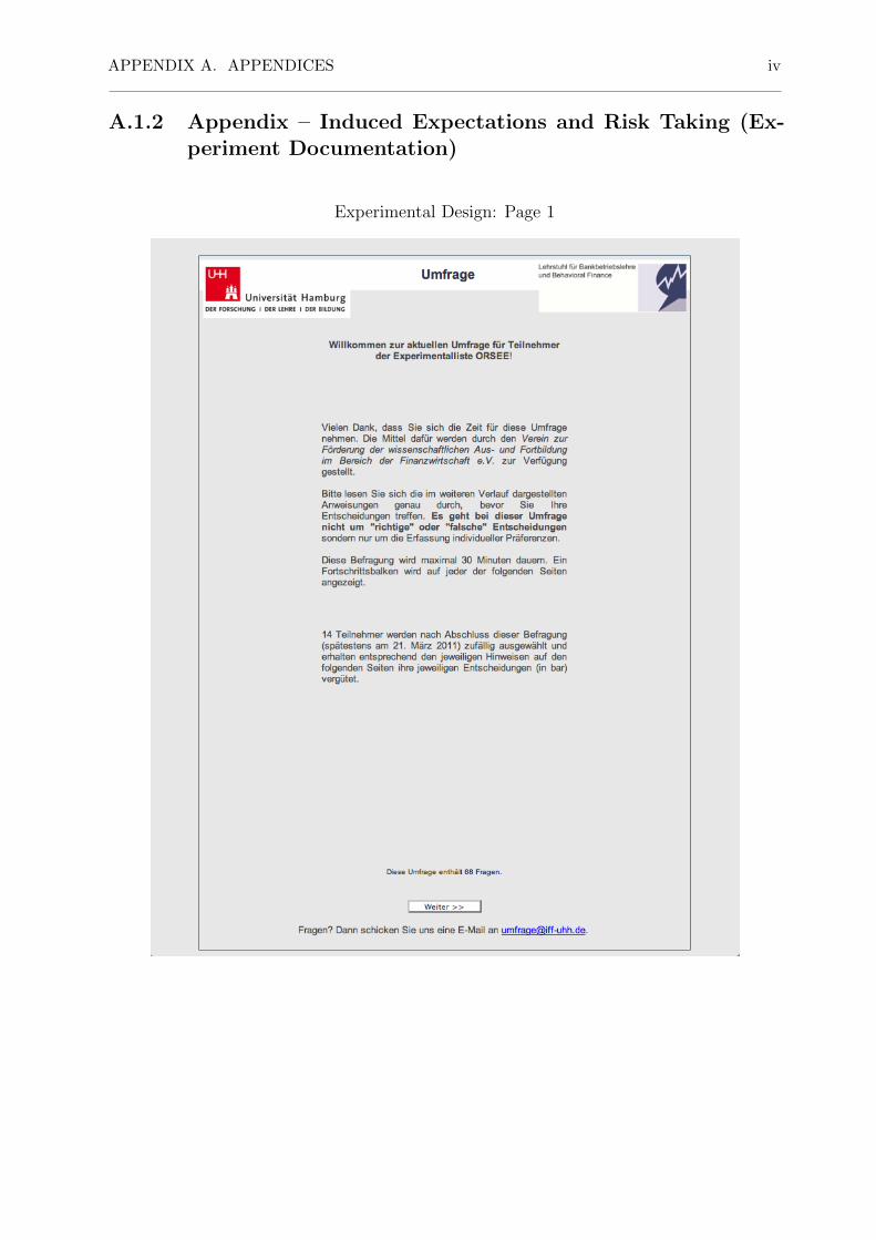
APPENDIX A. APPENDICES iv
A.1.2 Appendix – Induced Expectations and Risk Taking (Ex-periment Documentation)
Experimental Design: Page 1

AP
PE
ND
IXA
.A
PP
EN
DIC
ES
v
Experimental Design: Empirics I

AP
PE
ND
IXA
.A
PP
EN
DIC
ES
vi
Experimental Design: Questions of Understanding I (Main Task I)

AP
PE
ND
IXA
.A
PP
EN
DIC
ES
vii
Experimental Design: Questions of Understanding II (Main Task I)

APPENDIX A. APPENDICES viii
Experimental Design: Main Task I
10 decision tasks: modified Holt and Laury lotteries with fixed amount of 3.5 for each stage

AP
PE
ND
IXA
.A
PP
EN
DIC
ES
ix
Experimental Design: Empirics II
We captured additional empirics, financial background and self-assessement of statistical knowledge.

AP
PE
ND
IXA
.A
PP
EN
DIC
ES
x
Experimental Design: Questions of Understanding (Main Task II)
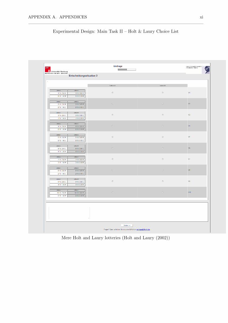
APPENDIX A. APPENDICES xi
Experimental Design: Main Task II – Holt & Laury Choice List
Mere Holt and Laury lotteries (Holt and Laury (2002))

AP
PE
ND
IXA
.A
PP
EN
DIC
ES
xii
Experimental Design: Big Five Questionnaire (Caprara et al. (1993))

AP
PE
ND
IXA
.A
PP
EN
DIC
ES
xiii
Experimental Design: Questions of Understanding (Main Task III)
Modified Holt and Laury lotteries (Holt and Laury (2002)) – 10 draws with replacement

APPENDIX A. APPENDICES xiv
Experimental Design: Main Task III – modified Holt & Laury Choice List
10 draws with replacement

APPENDIX A. APPENDICES xv
Experimental Design: Questionnaire – Financial Literacy
Measure for financial literacy according to Noth and Puhan (2009)

AP
PE
ND
IXA
.A
PP
EN
DIC
ES
xvi
Experimental Design: Questions of Understanding (Main Task IV)

APPENDIX A. APPENDICES xvii
Experimental Design: Main Task IV – modified Holt & Laury Choice List
all amounts multiplied by factor 10

AP
PE
ND
IXA
.A
PP
EN
DIC
ES
xviii
Experimental Design: Self Assessment Risk Taking

APPENDIX A. APPENDICES xix
Experimental Design: Questionnaire Preferences for Consistency
Measure for preferences for consistency according to Cialdini et al. (1995)

APPENDIX A. APPENDICES xx
Experimental Design: Last Instructions and Information

APPENDIX A. APPENDICES xxi

APPENDIX A. APPENDICES xxii
A.2 Appendix – Risk Taking and Compensation Schemes
(Experiment Documentation)
Experimental Design: Page 1 and Empirics
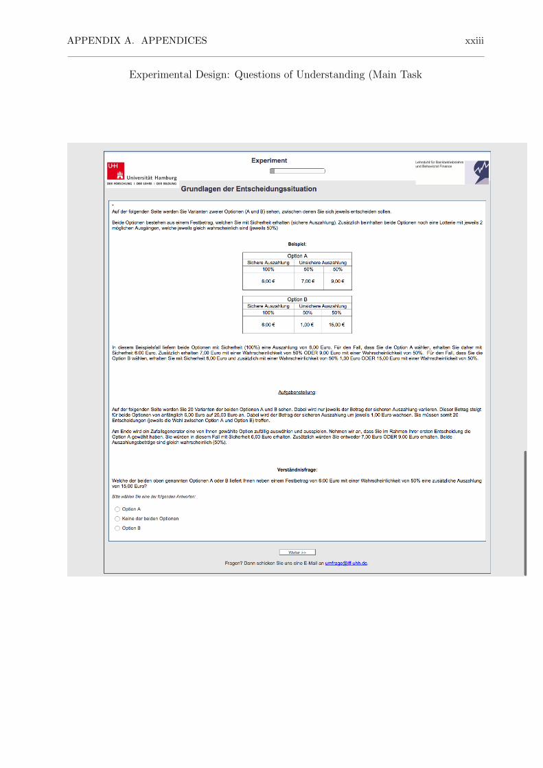
APPENDIX A. APPENDICES xxiii
Experimental Design: Questions of Understanding (Main Task

APPENDIX A. APPENDICES xxiv
Experimental Design: First Main Task
. . .
. . .
. . .
. . .
20 decision tasks: fixed amount from 6 euros to 25 euros by steps of 1 euro.

APPENDIX A. APPENDICES xxv
Experimental Design: Empirics
We captured additional empirics, financial background and self-assessement of statisticalknowledge

APPENDIX A. APPENDICES xxvi
Experimental Design: Big Five Questionnaire

APPENDIX A. APPENDICES xxvii
Experimental Design: Financial Literacy

APPENDIX A. APPENDICES xxviii
Experimental Design: Question of Understanding Holt & Laury Choice List

APPENDIX A. APPENDICES xxix
Experimental Design: Second Main Task – Holt & Laury Choice List

APPENDIX A. APPENDICES xxx
Experimental Design: Questionnaire Preferences for Consistency

APPENDIX A. APPENDICES xxxi
Last Instructions and Information

APPENDIX A. APPENDICES xxxii
A.3 Appendix – Asset Management of German Foun-
dations
A.3.1 Regulatory Main Principles for German Foundations
According to Huttemann and Schon (2007) §80 Abs. 2 S. 1 BGB constitutes both regulatorymain principles of the German foundation law: (1) preservation of the endowment, (2)generating revenues in order to permanently fulfill the foundations purposes.
§80 BGB Entstehung einer rechtsfahigen Stiftung(1) Zur Entstehung einer rechtsfahigen Stiftung sind das Stiftungsgeschaft und die Anerken-nung durch die zustandige Behorde des Landes erforderlich, in dem die Stiftung ihren Sitzhaben soll.(2) Die Stiftung ist als rechtsfahig anzuerkennen, wenn das Stiftungsgeschaft den Anforderun-gen des §81 Abs. 1 genugt, die dauernde und nachhaltige Erfullung des Stiftungszwecksgesichert erscheint und der Stiftungszweck das Gemeinwohl nicht gefahrdet. Bei einerStiftung, die fur eine bestimmte Zeit errichtet und deren Vermogen fur die Zweckverfol-gung verbraucht werden soll (Verbrauchsstiftung), erscheint die dauernde Erfullung desStiftungszwecks gesichert, wenn die Stiftung fur einen im Stiftungsgeschaft festgelegtenZeitraum bestehen soll, der mindestens zehn Jahre umfasst.(3) Vorschriften der Landesgesetze uber kirchliche Stiftungen bleiben unberuhrt. Dasgilt entsprechend fur Stiftungen, die nach den Landesgesetzen kirchlichen Stiftungen gle-ichgestellt sind.

APPENDIX A. APPENDICES xxxiii
A.3.2 German Translation of Table 4.1
Table A.1: Preservation Principles of the German Federal States
Reichweite des Prinzips derVermogenserhaltung
Bundesland
Der Bestand ist zu erhalten. Baden-Wuertemberg, Sachsen-Anhalt, Schleswig-Holstein, Thurin-gen
Der Bestand ist ungeschmalert zuerhalten.
Bayern, Berlin, Bremen, Hessen,Niedersachsen, Nordrhein-Westfalen,Saarland
Der Bestand ist moglichst. Hamburg, Rheinland-Pfalz
Der ist wertmaßig und in seiner Er-tragskraft zu erhalten
Sachsen
Keine Vorgaben Brandenburg, Mecklenburg-Vorpommern

APPENDIX A. APPENDICES xxxiv
A.3.3 Extracts from Federal State Foundation Laws
Below, we display these parts of the federal states foundation-laws which directly refer tothe preservation of the endowment and the asset management. The complete legislativetexts can be found at:http://www.stiftungen.org/de/stiftungswissen/recht-und-steuern/landesstiftungsgesetze.html
Foundation-Law Baden-Wurttemberg (in the version of December 16, 2003)§7 - Stiftungsverwaltung, Stiftungsvermogen(1) Die Stiftung ist nach den Gesetzen, dem Stiftungsgeschaft und der Stiftungssatzungsparsam und wirtschaftlich zu verwalten. Die Verwaltung dient der dauernden und nach-haltigen Erfullung des Stiftungszwecks.(2) Das Stiftungsvermogen ist in seinem Bestand zu erhalten, es sei denn, dass die Satzungeine Ausnahme zulasst oder der Stifterwille nicht anders zu verwirklichen ist; der Bestandder Stiftung muss auch in diesen Fallen fur angemessene Zeit gewahrleistet sein. DasStiftungsvermogen ist von anderen Vermogen getrennt zu halten.
Foundation-Law Bayern (in the version of September 26, 2008)Artikel 6 - Verwaltung der Stiftungen(1) Das Vermogen der Stiftung ist sicher und wirtschaftlich zu verwalten. Es ist vomVermogen anderer Rechtstrager getrennt zu halten. Es darf unter keinem Vorwand demVermogen des Staates, einer Gemeinde, eines Gemeindeverbands oder einer sonstigenKorperschaft oder Anstalt des offentlichen Rechts einverleibt werden. Der Anfall desVermogens aufgehobener Stiftungen wird dadurch nicht beruhrt.(2) Das Vermogen, das der Stiftung zugewendet wurde, um aus seiner Nutzung denStiftungszweck dauernd und nachhaltig zu erfullen (Grundstockvermogen), ist ungeschmalertzu erhalten.(3) Ertrage des Vermogens der Stiftung und zum Verbrauch bestimmte Zuwendungen durfennur zur Erfullung des Stiftungszwecks verwendet werden. Die Zufuhrung von Ertragen zumGrundstockvermogen, um dieses in seinem Wert zu erhalten, bleibt hiervon unberuhrt.

APPENDIX A. APPENDICES xxxv
Foundation-Law Berlin (in the version of July 22, 2003)§3Das Stiftungsvermogen ist in seinem Bestand ungeschmalert zu erhalten. Das Stiftungs-geschaft oder die Satzung kann Ausnahmen zulassen.
Foundation-Law Bremen (in the version of Feburary 27, 2007)§7 - Stiftungsvermogen und Ertrage(1) Das Stiftungsvermogen ist in seinem Bestand ungeschmalert zu erhalten. Die Stiftungs-behorde kann Ausnahmen zulassen, wenn der Stifterwille anders nicht zu verwirklichen istund der Bestand der Stiftung fur angemessene Zeit gewahrleistet ist.(2) Das Stiftungsvermogen ist von anderem Vermogen getrennt zu halten.(3) Die Ertrage des Stiftungsvermogens und Zuwendungen an die Stiftung sind ausschließlichfur den Stiftungszweck und zur Deckung der notwendigen Verwaltungskosten der Stiftungzu verwenden; die Verwendung fur den Stiftungszweck schließt die Bildung angemessenerRucklagen ein. Sie konnen dem Stiftungsvermogen zugefuhrt werden, soweit es die Satzungvorsieht oder zur Erhaltung des Stiftungsvermogens in seinem Wert angezeigt ist. Zuwen-dungen sind dem Stiftungsvermogen zuzufuhren, wenn der Zuwendende es bestimmt.(4) Reichen Stiftungsertrage und Zuwendungen zur Erfullung des Stiftungszwecks nicht aus,so sollen sie dem Stiftungsvermogen zugefuhrt werden, sofern erwartet werden kann, dassaus den Ertragen des vergroßerten Stiftungsvermogens in absehbarer Zeit der Stiftungszwecknachhaltig erfullt werden kann.
Foundation-Law Hamburg (in the version of December 14, 2005)§4 - Vermogen und Verwaltung der Stiftung(1) Die Stiftungsorgane haben nach Maßgabe des Stifterwillens fur die dauernde undnachhaltige Verwirklichung des Stiftungszwecks zu sorgen.(2) Das Stiftungsvermogen ist von anderen Vermogen getrennt zu halten. Es ist sicher undertragbringend anzulegen; Umschichtungen sind in diesem Rahmen zulassig. Soweit nicht inder Satzung etwas anderes bestimmt ist, ist das Stiftungsvermogen moglichst ungeschmalertzu erhalten, es sei denn, der Stifterwille kann auf diese Weise nicht verwirklicht werden.(3) Soweit nicht in der Satzung etwas anderes bestimmt ist, sind die Ertrage des Stiftungsvermogensund die nicht ausdrucklich zum Vermogen gewidmeten Zuwendungen Dritter nach Abzugder notwendigen Verwaltungskosten zur Verwirklichung des Stiftungszwecks zu verwen-den. Rucklagen konnen gebildet werden, soweit dies der nachhaltigen Verwirklichung desStiftungszwecks dient und die Satzung nicht entgegensteht.(4) Die Stiftung hat jahrlich eine Jahresrechnung mit einer Vermogensubersicht und einemBericht uber die Erfullung des Stiftungszwecks zu erstellen; die Grundsatze ordnungsmaßigerBuchfuhrung sind entsprechend anzuwenden.
Foundation-Law Hessen (in the version of September 6, 2007)§6 Stiftungsvermogen(1) Das Stiftungsvermogen ist in seinem Bestand ungeschmalert zu erhalten. Die Aufsichts-behorde kann Ausnahmen zulassen, wenn der Stifterwille anders nicht zu verwirklichenund der Bestand der Stiftung fur angemessene Zeit gewahrleistet ist(2) Das Stiftungsvermogen ist von anderem Vermogen getrennt zu halten.(3) Der Ertrag des Stiftungsvermogens und Zuwendungen durfen nur entsprechend demStiftungszweck verwendet werden. Das gleiche gilt im Falle des Abs. 1 Satz 2 fur dasStiftungsvermogen.

APPENDIX A. APPENDICES xxxvi
Foundation-Law Niedersachsen (in the version of November 23, 2004)§6 Verwaltung der Stiftung(1) Das Stiftungsvermogen ist in seinem Bestand ungeschmalert zu erhalten. Die Stiftungs-behorde kann Ausnahmen zulassen, wenn der Stifterwille anders nicht zu verwirklichen undder Bestand der Stiftung fur angemessene Zeit gewahrleistet ist. Das Stiftungsvermogenist von anderem Vermogen getrennt zu halten.(2) Die Ertrage des Stiftungsvermogens sind ausschließlich fur den Stiftungszweck zu ver-wenden. Sie durfen dem Stiftungsvermogen zugefuhrt werden, wenn es die Satzung vorsiehtoder wenn es zum Ausgleich von Vermogensverlusten erforderlich ist. Zuwendungen andie Stiftung sind fur den Stiftungszweck zu verwenden, soweit sie nicht ausdrucklich demStiftungsvermogen zugefuhrt werden sollen.(3) Die Mitglieder der Stiftungsorgane sind zur ordnungsmaßigen Verwaltung der Stiftungverpflichtet. Organmitglieder, die ihre Pflichten schuldhaft verletzen, sind der Stiftungzum Ersatz des daraus entstehenden Schadens verpflichtet. Die Haftung wegen groberFahrlassigkeit kann nicht ausgeschlossen werden.(4) Die Verwaltungskosten sind auf ein Mindestmaß zu beschranken. Die Mitglieder derStiftungsorgane haben Anspruch auf Ersatz angemessener Auslagen. Bei entgeltlicherTatigkeit von Organmitgliedern sind Art und Umfang der Dienstleistungen und derVergutung vor Aufnahme der Tatigkeit schriftlich zu regeln. Ist eine Behorde Stiftungsor-gan, so hat die Stiftung im Zweifel nur die Auslagen zu ersetzen.
Foundation-Law Nordrhein-Westfalen (in the version of Feburary 15, 2005)§4 Grundsatze (1) Die Stiftungsorgane haben die Stiftung so zu verwalten, wie es diedauernde und nachhaltige Verwirklichung des Stiftungszwecks im Sinne der Stiftungssatzungoder - hilfsweise - des mutmaßlichen Willens der Stifterin oder des Stifters erfordert.(2) Soweit nicht in der Satzung etwas anderes bestimmt ist oder der Wille der Stifterin oderdes Stifters auf andere Weise nicht verwirklicht werden kann, ist das Stiftungsvermogenungeschmalert zu erhalten. Vermogensumschichtungen sind nach den Regeln ordentlicherWirtschaftsfuhrung zulassig.(3) Soweit nicht in der Satzung etwas anderes bestimmt ist, sind die Ertrage des Stiftungsvermogenssowie Zuwendungen Dritter, die nicht ausdrucklich zur Erhohung des Stiftungsvermogensbestimmt sind, zur Verwirklichung des Stiftungszwecks und zur Deckung der Verwal-tungskosten zu verwenden.
Foundation-Law Rheinland-Pfalz (in the version of July 19, 2004)§7 - Verwaltung der Stiftung(1) Die Stiftungsorgane haben nach Maßgabe des Stifterwillens fur die dauernde undnachhaltige Verwirklichung des Stiftungszwecks zu sorgen.(2) Soweit nicht in der Satzung etwas anderes bestimmt ist oder der Stifterwille auf andereWeise nicht verwirklicht werden kann, ist das Stiftungsvermogen moglichst ungeschmalertzu erhalten; Umschichtungen des Stiftungsvermogens sind nach den Regeln ordentlicherWirtschaftsfuhrung zulassig. Das Stiftungsvermogen ist von anderem Vermogen getrenntzu halten.(3) Soweit nicht in der Satzung etwas anderes bestimmt ist, sind die Ertrage des Stiftungsvermogensund die nicht zu seiner Erhohung bestimmten Zuwendungen Dritter zur Verwirklichung desStiftungszwecks und zur Deckung der Verwaltungskosten zu verwenden. Die Ertrage konnenauch dem Stiftungsvermogen zugefuhrt werden, soweit dies der nachhaltigen Verwirklichung

APPENDIX A. APPENDICES xxxvii
des Stiftungszwecks dient.(4) Die Stiftung hat innerhalb von sechs Monaten nach Schluss des Geschaftsjahres eineJahresrechnung mit einer Vermogens- ubersicht und einem Bericht uber die Erfullung desStiftungszwecks zu erstellen.
Foundation-Law Saarland (in the version of August 9, 2004)§6 - Stiftungsvermogen(1) Das Stiftungsvermogen ist in seinem Bestand ungeschmalert zu erhalten. Die Stiftungs-behorde kann Ausnahmen zulassen, wenn der Stifterwille anders nicht zu verwirklichen undder Bestand der Stiftung fur angemessene Zeit gewahrleistet ist. Das Stiftungsvermogenist von anderem Vermogen getrennt zu halten. (2) Die Ertrage des Stiftungsvermogensund Zuwendungen an die Stiftung sind ausschließlich fur den Stiftungszweck und zurDeckung der Verwaltungskosten der Stiftung sowie zur Bildung angemessener Rucklagen zuverwenden. Sie konnen dem Stiftungsvermogen zugefuhrt werden, wenn es in der Satzungvorgesehen oder im Einzelfalle notwendig ist, um die Ertragskraft des Vermogens auch inZukunft sicherzustellen. Zuwendungen mussen dem Stiftungsvermogen zugefuhrt werden,wenn Zuwendende es bestimmen (Zustiftung).
Foundation-Law Sachsen (in the version of August 7, 2004)§4 - Stiftungsverwaltung(1) Die Stiftung ist zur dauernden und nachhaltigen Erfullung des Stiftungszwecks sparsamund wirtschaftlich zu verwalten.(2) Die Stiftung hat nach den Grundsatzen ordnungsmaßiger Buchfuhrung Rechnung zufuhren.(3) Das Stiftungsvermogen ist wertmaßig in seinem Bestand und seiner Ertragskraft zuerhalten, es sei denn, dass die Satzung oder die Stiftungsbehorde eine Ausnahme zulasstund der Stiftungszweck nicht anders zu verwirklichen ist. Das Stiftungsvermogen ist vonanderem Vermogen getrennt zu halten.
Foundation-Law Sachsen-Anhalt (in the version of Januar 20, 2011)§7 - Pflichten der Stiftung(1) Die Stiftung hat ihr Vermogen im Einklang mit den Rechtsvorschriften und dem inStiftungsgeschaft und Stiftungssatzung zum Ausdruck kommenden Stifterwillen nach denRegeln ordentlicher Wirtschaftsfuhrung zu verwalten. Die Verwaltung dient der dauerndenund nachhaltigen Erfullung des Stiftungszwecks.(2) Das Vermogen, das der Stiftung zugewendet wurde, um aus seiner Nutzung denStiftungszweck nachhaltig zu erfullen (Grundstockvermogen), ist in seinem Bestand zuerhalten, es sei denn, dass der Stiftungszweck anders nicht zu erfullen ist. Das Grund-stockvermogen ist vom ubrigen Vermogen getrennt zu halten. Der Bestand und seine Ver-anderungen sind gesondert nachzuweisen.(3) Die Ertrage des Grundstockvermogens und diejenigen Zuwendungen Dritter, die nichtausdrucklich zur Erhohung des Grundstockvermogens bestimmt sind, sind zur Erfullungdes Stiftungszwecks zu verwenden.(4) Die Stiftung ist verpflichtet, der Aufsichtsbehorde 1. die Zusammensetzung der Organe,2. die zur Vertretung Befugten nebst deren ladungsfahigen Anschriften und 3. Anderungender Angaben nach den Nummern 1 und 2 innerhalb einer Frist von einem Monat nachEintritt der Wirksamkeit mitzuteilen. Die Stiftung hat der Aufsichtsbehorde ferner jed-erzeit auf Verlangen Auskunfte zu erteilen sowie Geschafts- und Kassenbucher, Akten undsonstige Unterlagen zur Einsichtnahme vorzulegen.

APPENDIX A. APPENDICES xxxviii
(5) Die Stiftung ist verpflichtet, der Aufsichtsbehorde innerhalb von zwolf Monaten nachAblauf des Geschaftsjahres eine Jahresrechnung mit einer Vermogensubersicht und einenBericht uber die Erfullung des Stiftungszwecks (Rechnungsabschluss) vorzulegen.(6) Wird die Stiftung durch einen Wirtschaftsprufer, einen vereidigten Buchprufer, eineWirtschaftsprufergesellschaft, eine Buchprufungsgesellschaft, einen Pru- fungsverband odereine Behorde gepruft, so ist anstelle der Jahresrechnung und der Vermogensubersichtder Prufungsbericht einzureichen. Die Prufung hat sich auch auf die satzungsgemaßeVerwendung der Stiftungsmittel und die Erhaltung des Grundstockvermogens zu erstrecken.Das Ergebnis der Prufung ist in einem Abschlussvermerk des Prufers festzuhalten.
Foundation-Law Schleswig-Holstein (in the version of October 12, 2005)§4 - Verwaltung der Stiftung(1) Die zur Verwaltung der Stiftung berufenen Organe haben fur die dauernde und nach-haltige Erfullung des Stiftungszwecks zu sorgen.(2) Das der Stiftung zur dauernden und nachhaltigen Erfullung des Stiftungszwecks zuge-wandte Vermogen (Stiftungsvermogen) ist in seinem Bestand zu erhalten, es sei denn, dassdie Satzung eine Ausnahme zulasst oder der Stifterwille anders nicht zu verwirklichen ist.Das Stiftungsvermogen ist von anderem Vermogen getrennt zu halten.(3) Die Ertrage des Stiftungsvermogens sowie die Zuwendungen von Dritten sind fur denStiftungszweck und die notwendigen Verwaltungskosten der Stiftung zu verwenden. Diesgilt jedoch nicht fur Zuwendungen von Dritten, die nach dem Willen der oder des Zuwen-denden dazu bestimmt sind, dem Stiftungsvermogen zugefuhrt zu werden (Zustiftungen).Diese werden Bestandteil des Stiftungsvermogens nach Absatz 2 Satz 1.(4) Die Stiftungsorgane konnen Ertrage dem Stiftungsvermogen zufuhren, sofern diesnotwendig ist, um die Ertragskraft des Stiftungsvermogens auch in Zukunft sicherzustellen,oder soweit sie im Einzelfall zur Erfullung des Stiftungszwecks keine Verwendung finden.Dies gilt auch fur Zuwendungen von Dritten, sofern dies nicht deren erklartem Willenwiderspricht.(5) Ist das Stiftungsvermogen einer Stiftung derart geschwacht, dass die nachhaltigeErfullung des Stiftungszwecks nicht mehr gewahrleistet erscheint, so kann die zustandigeBehorde schriftlich anordnen, dass die Ertrage des Stiftungsvermogens ganz oder teilweiseso lange anzusammeln und dem Stiftungsvermogen zuzufuhren sind, bis die Stiftung wiederleistungsfahig ist.(6) Sind die Mitglieder der Stiftungsorgane nicht hauptamtlich zur Verwaltung der Stiftungberufen, kann die Satzung 1.den Ersatz ihrer notwendigen Auslagen und ihres entgangenenArbeitsverdienstes oder 2.die Gewahrung einer angemessenen Aufwandsentschadigungvorsehen.(7) uber den Bestand und die Veranderungen des Stiftungsvermogens sowie alle Einnahmenund Ausgaben der Stiftung ist ordnungsgemaß Buch zu fuhren.
Foundation-Law Thuringen (in the version of December 16, 2008)§8 - Verwaltung und Rechnungslegung der Stiftung(1) Die Stiftungsorgane haben die Stiftung sparsam und nach den Regeln ordentlicherWirtschaftsfuhrung zu verwalten. Die Verwaltung dient der dauernden und nachhaltigenVerwirklichung des Stiftungszwecks.(2) Das Stiftungsvermogen ist in seinem Bestand zu erhalten, es sei denn, dass die Satzungeine Ausnahme zulasst, der Stiftungszweck anders nicht zu verwirklichen ist und die Dauer-haftigkeit der Stiftung gewahrleistet bleibt. Das Stiftungsvermogen sowie Veranderungen

APPENDIX A. APPENDICES xxxix
in seinem Bestand sind getrennt von anderen Vermogensmassen gesondert nachzuweisen.(3) Die Ertrage des Stiftungsvermogens sind zur Verwirklichung des Stiftungszwecks sowiefur die entstehenden Verwaltungskosten zu verwenden. Gleiches gilt fur ZuwendungenDritter, die nicht ausdrucklich zur Erhohung des Stiftungsvermogens bestimmt sind, soweitin der Satzung nicht etwas anderes bestimmt ist.

Appendix B
General Appendix
xl

APPENDIX B. GENERAL APPENDIX xli
B.1 Abstracts and Current Status of Papers (§6 (5)
PromO)
Chapter 2: Risk Taking and Induced Reference Points
Abstract (English) Based on the model of Koszegi and Rabin (2007) (KR) and theassumption that expectations can determine the reference point and thus risk taking, weconduct an experiment. We transfer the results provided by Abeler et al. (2011), whoprovide experimental evidence for the model of KR, from the field of work performance toindividual risk taking. By controlling the expectations of our subjects we can show thatinduced expectations can have a significant impact on individual willingness to take risks.
Abstract (German) Ausgehend von dem theoretischen Modell von Koszegi and Ra-bin (2007) und deren Annahme, dass Erwartungen den Referenzpunkt und damit dasRisikoverhalten beeinflussen konnen, fuhren wir eine experimentelle Untersuchung dieserFrage durch. Wir ubertragen dazu die Ergebnisse von Abeler et al. (2011), die diesesModell fur den Bereich der Arbeitsleistung experimentell validieren konnen, auf den Bereichder Risikoubernahme. Wir konnen zeigen, dass unter kontrollierten Erwartungen, dieBereitschaft Risiken einzugehen, durch das gezielte Induzieren einer Erwartungshaltungsignifikant beeinflusst werden kann.
Current Status Working Paper
APPENDIX B. GENERAL APPENDIX xlii
Chapter 3: Risk Taking and Compensation Schemes
Abstract (English) Motivated by recent regulatory initiatives in the financial sectorsuch as bonus caps, we conduct a risk taking experiment and show that a shift in thestructure of executive remuneration can increase the willingness to take risks. By graduallyincreasing the fixed component of total compensation, subjects switch from choosing alow variance lottery to a high variance lottery. More than half of our subjects revealEUT-inconsistent choice behavior. This behavior can be explained by reference dependentpreferences, with the fixed salary serving as reference point.
Abstract (German) Ausgehend von jungsten regulatorischen Maßnahmen im Finanzsek-tor, wie insbesondere die Deckelung von Bonuszahlungen und der einhergehenden Erhohungder Festgehalter durch die Finanzinstitute, fuhren wir ein Experiment durch. Wir konnenzeigen, dass ein solcher Eingriff in die Vergutungsstruktur, die Bereitschaft Risiken einzuge-hen, erhohen kann. Im Rahmen der Versuchsanordnung erhohen wir schrittweise die fixeGehaltskomponente und konnen zeigen, dass mehr als die Halfte unserer Versuchsper-sonen ein Verhalten offenbaren, welches die Vorhersagen der Erwartungsnutzen-Theorieverletzt. Dieses Verhalten lasst sich mit referenzabhangigen Praferenzen erklaren, wobeidas Festgehalt als Referenzpunkt dient.
Current Status Working Paper

APPENDIX B. GENERAL APPENDIX xliii
Chapter 4: Asset Management of German Foundations
Abstract (English) This study has two objectives. First, we define a legal and financialframework for the asset management of German non-profit foundations. Second, we deriveasset management strategies within this framework in order to compare different approachesand test their suitability for the purposes of German non-profit foundations by meansof stochastic simulations. We find that simple heuristics such as GDP-weighted stockportfolios suggested by Jacobs et al. (2014) provide superior results in comparison withempiric asset allocations. Additionally, we calculate potential welfare losses resulting frominefficient (empirical) investment behavior.
Abstract (German) Diese Studie hat zwei Ziele. Zunachst definieren wir einen rechtlichenund finanzwirtschaftlichen Handlungsrahmen fur die Vermogensverwaltung von deutschengemeinnutzigen Stiftungen. Im Anschluss leiten wir unterschiedliche Anlagestrategien ab,welche diesen rechtlichen Kriterien unterliegen. Wir zeigen, dass einfache Heuristiken, wiez.B. die von Jacobs et al. (2014) vorgeschlagene Gewichtung von Aktien mittels des BIP,Ergebnisse liefern, die den empirisch belegbaren Anlagestrategien deutscher Stiftungenuberlegen sind. Wir vergleichen diese Strategien mit empirischen Vermogensallokationendeutscher Stiftungen und berechnen die sich daraus ergebenen moglichen Verluste fur dieWohlfahrt.
Current Status Working Paper

APPENDIX B. GENERAL APPENDIX xliv
B.2 Statement of Personal Contribution (§6 (3) PromO)
Main Tasks
Chapter Co-Author Design Execution Reporting
2 Markus Noth Review of literature
Development of researchquestion
Design of the experimentalmain setup (i.e., adaptionof Holt and Laurylotteries)
Supplement of theexperimental main setup(i.e., query of personalityfactors: Big-Five factormodel) (S)
Testing and debugging ofexperiment (S)
Conducting of experiment
Preparation of data
Raising of funds forexperiment (S)
Interpretation anddiscussion of results
Drawing up of workingpaper
Presentation of results atconferences and researchseminars
3 Review of literature
Development of researchquestion
Design of the experimentalsetup
Testing and debugging ofexperiment
Conducting of experiment
Preparation of data
Raising of funds forexperiment (S)
Interpretation anddiscussion of results
Drawing up of workingpaper
Presentation of results atconferences and researchseminars
4 Review of literature
Development of researchquestion
Choice of methodology(stochastic simulations)
Selection and procurementof raw data
Preparation of data
Running of stochasticsimulations
Interpretation anddiscussion of results
Drawing up of workingpaper
Presentation of results atconferences and researchseminars
Note: Tasks followed by (S) were performed in partnership with supervisor Markus Noth.

APPENDIX B. GENERAL APPENDIX xlv
B.3 Affidavit (§6 (4) PromO)
Hiermit erklare ich, Roger Gothmann, an Eides statt, dass ich die Dissertation mit demTitel: Essays on Individual and Institutional Willingness to Take Risks
selbststandig und bei einer Zusammenarbeit mit anderen Wissenschaftlern gemaß derbeigefugten Darlegung nach §6 (3) der Promotionsordnung der Fakultat Wirtschafts- undSozialwissenschaften vom 24. August 2010 verfasst und keine anderen als die von mirangegebenen Hilfsmittel benutzt habe. Die den herangezogenen Werken wortlich odersinngemaß entnommenen Stellen sind als solche gekennzeichnet.
Ich versichere, dass ich keine kommerzielle Promotionsberatung in Anspruch genommenhabe und die Arbeit nicht schon in einem fruheren Promotionsverfahren im In- oder Auslandangenommen oder als ungenugend beurteilt worden ist.
Hamburg, 13. Februar 2019 Roger Gothmann