essays on gcc energy economics and saudi arabia’s
TRANSCRIPT

Essays on GCC Energy Economics and Saudi Arabia’s Economic Growth
by
Mohammed Al Mahish
A dissertation submitted to the Graduate Faculty of
Auburn University
in partial fulfillment of the
requirements for the Degree of
Doctor of Philosophy
Auburn, Alabama
December 10, 2016
Keywords: GCC, Energy Subsidy, Electricity, Technical Change, Economic Growth, Saudi Arabia
Copyright 2016 by Mohammed Al Mahish
Approved by
Curtis Jolly, Chair, Alumni and Barkley Endowed Professor of Agricultural Economics
Patricia Duffy, Professor of Agricultural Economics
Norbert Wilson, Professor of Agricultural Economics
Daowei Zhang, Alumni and George W. Peake Professor of Forest Economics

ii
Abstract
The first chapter analyzes the impact of energy subsidies on a select sample of nitrogen
fertilizer producers in the Arabian Gulf Cooperation Council (GCC) region that disclose their
financial statements. The paper estimates ammonia production costs per ton in the GCC region
ranging from $53 to $116, and urea production costs ranging from $56.64 to $102.28 using Yara’s
method. Using Budidarm’s method, the production cost for a ton of urea is estimated to range from
$86.25 to $152.50. The differences in cost are attributed to differences in calculation methods.
Subsidies for the selected sample were estimated using the price gap approach. Subsidy rates were
on average well above 50% and subsidy size reaches billions of dollars. The paper then develops
a translog multi-output, multi-input restricted profit function to evaluate the impact of the energy
subsidy and international natural gas prices on inputs demand, outputs supply, and profit of the
GCC producers. Results show that output supply, input demand, and profit are highly responsive
to changes in urea prices. The results also show that international natural gas prices have an
inelastic positive impact on the GCC firms’ profit. The study concluded that despite the distorting
effect of subsidies in output supply and input demand, subsidy policy in the GCC region has
achieved one of its major goals by increasing demand for labor. Furthermore, the GCC corporate
nitrogen fertilizer executives’ concern that a reduction in the energy subsidy would have an adverse
effect on their companies’ profitability has been confirmed in this paper to be a valid concern.
The second chapter aims to accomplish two objectives. The first is to extend the existing
method of total factor productivity growth decomposition by incorporating network
iii
characteristics. The second objective is to empirically evaluate technical change and productivity
of the Saudi electricity sector. The results show that the Saudi electricity sector operates under the
presence of economies of output density, economies of customer density, and diseconomies of
scale. The technology used in the Saudi electricity sector is a cost saving technology. It is
characterized as fuel using, capital neutral, and energy saving technology. The estimated average
technical change term is positive. It indicates a cost increase during the timeframe of this study.
The estimated average total factor productivity growth is positive using both the proposed and
existing method. Compared with the proposed method, the existing method overestimated total
factor productivity growth of the Saudi electricity sector. Furthermore, the paper estimated an
optimal scale of output to be almost 11 percent larger than the maximum output level generated
by the Saudi Electricity Company. The paper concludes that the Saudi Electricity Company needs
to expand its size to reach the optimal output level.
The third chapter investigates the impact of the overall financing activities on economic
growth in Saudi Arabia. The study developed a financing index that takes into account the overall
available credit in Saudi Arabia. The index was shown to be sensitive to economic and political
shocks such as the Arab Spring. Using Johnson cointegration approach, the paper found an
evidence of a long run relationship between real GDP per capita, financing, real interest rate, public
labor force, and capital. Using a vector error correction model, the paper found a robust estimate
that proves the positive impact of financing on economic growth in Saudi Arabia. Furthermore,
the Granger-Causality Wald test indicates that financing influences economic growth in Saudi
Arabia.

iv
Acknowledgments
I would like to thank my father for encouraging me to pursue graduate studies and for his
constant support. I also would like to thank my mother for her caring and motivation. I also would
like to thank my wife for her passion, kindness, and patience during my doctoral studies in the US.
Also, I thank my brothers and sisters for keeping in touch with me during my graduate studies in
the US and for their continuous support.
I really thank and appreciate my advisor, Dr. Jolly, for his outstanding supervision. Dr.
Jolly’s advices and suggestions have helped me not only in my academic studies but also in my
career. I appreciate and thank Dr. Duffy for her valuable comments and suggestions that have
greatly enhanced my dissertation. Thank you to Dr. Wilson and Dr. Zhang for serving on my
committee. Thank you to Dr. Banerjee for serving as the University Reader.
I appreciate and thank King Faisal University for providing me with an outstanding
scholarship to pursue my doctoral studies in the US. I also thank Saudi Arabian Cultural Mission
(SACM) for supervising my master’s and doctoral studies.

v
Table of Contents
Abstract ......................................................................................................................................... ii
Acknowledgments........................................................................................................................ iv
List of Tables ............................................................................................................................... vi
List of Illustrations ...................................................................................................................... vii
List of Abbreviations ................................................................................................................. viii
Chapter 1 ..................................................................................................................................... 1
1.1 Introduction ....................................................................................................................... 1
1.2 Literature Review.............................................................................................................. 3
1.3 Data ................................................................................................................................... 5
1.4 Economics of Fertilizers Production ................................................................................. 8
1.5 Model .............................................................................................................................. 12
1.6 Estimation and Results .................................................................................................... 17
1.7 Conclusion ...................................................................................................................... 27
Chapter 2 ................................................................................................................................... 29
2.1 Introduction ..................................................................................................................... 29
2.2 Literature Review............................................................................................................ 30
2.3 Methodology and Data .................................................................................................... 33
2.4 Model Estimation and Discussion .................................................................................. 41
2.5 Optimal Scale .................................................................................................................. 51

vi
2.6 Conclusion ...................................................................................................................... 51
Chapter 3 ................................................................................................................................... 53
3.1 Introduction ..................................................................................................................... 53
3.2 Literature Review............................................................................................................ 54
3.3 Model .............................................................................................................................. 59
3.4 Data ................................................................................................................................. 59
3.5 Financing Index .............................................................................................................. 60
3.6 Estimation Procedures and Results ................................................................................. 62
3.7 Robustness Check ........................................................................................................... 66
3.8 Conclusion ...................................................................................................................... 67
References ................................................................................................................................. 69
Appendix A ................................................................................................................................ 81
Appendix B ............................................................................................................................... 83

vii
List of Tables
Table 1.1 ...................................................................................................................................... 6
Table 1.2 ...................................................................................................................................... 8
Table 1.3 ...................................................................................................................................... 9
Table 1.4 .................................................................................................................................... 10
Table 1.5 .................................................................................................................................... 18
Table 1.6 .................................................................................................................................... 19
Table 1.7 .................................................................................................................................... 20
Table 1.8 .................................................................................................................................... 21
Table 1.9 .................................................................................................................................... 22
Table 1.10 .................................................................................................................................. 22
Table 2.1 .................................................................................................................................... 40
Table 2.2 .................................................................................................................................... 42
Table 2.3 .................................................................................................................................... 43
Table 2.4 .................................................................................................................................... 45
Table 2.5 .................................................................................................................................... 47
Table 2.6 .................................................................................................................................... 49
Table 2.7 .................................................................................................................................... 50
Table 2.8 .................................................................................................................................... 50
Table 3.1 .................................................................................................................................... 60

viii
Table 3.2 .................................................................................................................................... 61
Table 3.3 .................................................................................................................................... 64
Table 3.4 .................................................................................................................................... 65
Table 3.5 .................................................................................................................................... 67

ix
List of Illustrations
Figure 1.1 ..................................................................................................................................... 2
Figure 1.2 ..................................................................................................................................... 3
Figure 3.1 ................................................................................................................................... 54
Figure 3.2 ................................................................................................................................... 62

x
List of Abbreviations
GCC Gulf Cooperation Council
GMM Generalized Method of Moment
SAFCO Saudi Arabian Fertilizer Company
QAFCO Qatar Fertilizer Company
GPIC Gulf Petrochemicals Industries Company
PIC Petrochemical Industries Company
SEC Saudi Electricity Company
TFP Total Factor Productivity
EOS Economies of Scale
EOD Economies of Output Density
ECD Economies of Customer Density
SC Scale Component
TC Technical Change
SUR Seemingly Unrelated Regression
SAMA Saudi Arabia Monetary Agency
VECM Vector Error Correction Model
1
Chapter 1
The Impact of Energy Subsidy on Nitrogen Fertilizer Producers in
the GCC
1.1 Introduction
Nitrogen fertilizer consists of ammonia and urea. The main feedstock in the production of
ammonia is natural gas, and ammonia is used as a feedstock in the production of urea. The excess
ammonia production is usually sold domestically or exported. As reported by Huang (2007),
natural gas accounts for 72–85% of ammonia production cost; hence, natural gas cost is a major
variable cost in the production of nitrogen fertilizer.
The Gulf Cooperation Council (GCC) is composed of Saudi Arabia, United Arab Emirates,
Oman, Kuwait, Qatar, and Bahrain. Governments of these countries support their petrochemical
industries, including chemical fertilizer manufacturers, by providing them with natural gas prices
that are below international gas prices. The definition of subsidy by De Moor and Calamari1 (1997)
fits the type of subsidy given by the GCC governments to their fertilizer producers, since the
governmental support reduces the production costs. The purpose of this energy subsidy is
economic development through the utilization of local natural resources in providing the required
feedstock for mega industrial projects. This contributes to the national income diversification by
reducing the reliance on oil revenue, increasing the GDP, and reducing unemployment rate by
providing high quality employment opportunities for citizens. Another purpose of this energy
subsidy is to help local chemical and petrochemical corporations compete with international firms,
since the majority of the GCC petrochemicals and fertilizer production is exported to international
1 A subsidy is any measure that keeps prices for consumers below the market level or keeps prices for producers
above the market level, or that reduces costs for consumers and producers by giving direct or indirect support.

2
markets. Many corporate executives and energy subsidy advocates in the GCC region claim that
any increase in local subsidized natural gas prices will hinder their ability to compete in the
international market and will adversely impact their profit. They argue that other international
producers, such as Chinese producers, have a competitive advantage because they pay low wages.
The GCC nitrogen fertilizer capacity in 2011 reached almost 10% of the world total
production capacity (Markey, 2011). The GCC total nitrogen fertilizer production capacity in 2012
reached 26.7 million tons (GPCA, 2013). Figure 1.1 shows that Qatar and Saudi Arabia are among
ten of the largest urea producers in 2010. Three GCC countries (Saudi Arabia, Qatar, and Oman)
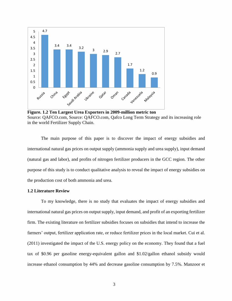
were among the 10 largest urea exporters in 2009, as shown in Figure 1.2. As for the largest urea
importers in 2009, India was first and the U.S. was second.
Figure. 1.1 Ten Largest Urea Producers in 2010- million metric ton
Source: QAFCO.com, Qafco Long Term Strategy and its increasing role in the world Fertilizer
Supply Chain.
54.7
21.8
7.13 5.5423.01
5.15 4.971 3.6 3.334 3.012
0
10
20
30
40
50
60
3
Figure. 1.2 Ten Largest Urea Exporters in 2009-million metric ton
Source: QAFCO.com, Source: QAFCO.com, Qafco Long Term Strategy and its increasing role
in the world Fertilizer Supply Chain.
The main purpose of this paper is to discover the impact of energy subsidies and
international natural gas prices on output supply (ammonia supply and urea supply), input demand
(natural gas and labor), and profits of nitrogen fertilizer producers in the GCC region. The other
purpose of this study is to conduct qualitative analysis to reveal the impact of energy subsidies on
the production cost of both ammonia and urea.
1.2 Literature Review
To my knowledge, there is no study that evaluates the impact of energy subsidies and
international natural gas prices on output supply, input demand, and profit of an exporting fertilizer
firm. The existing literature on fertilizer subsidies focuses on subsidies that intend to increase the
farmers’ output, fertilizer application rate, or reduce fertilizer prices in the local market. Cui et al.
(2011) investigated the impact of the U.S. energy policy on the economy. They found that a fuel
tax of $0.96 per gasoline energy-equivalent gallon and $1.02/gallon ethanol subsidy would
increase ethanol consumption by 44% and decrease gasoline consumption by 7.5%. Manzoor et
4.7
3.4 3.43.2
3 2.92.7
1.7
1.20.9
0
0.5
1
1.5
2
2.5
3
3.5
4
4.5
5

4
al. (2012) studied the impact of removing the energy subsidy in Iran using a computable general
equilibrium model suggesting that removing or eliminating energy subsidies that are part of
production will increase the cost of production for the overall economy. Hansen (2004) estimated
the Danish demand elasticity for nitrogen fertilizer using a generalized translog profit specification
to be -0.45. Fulginiti and Perrin (1990) analyzed the impact of Argentinean price and tax policies
on agricultural output growth rate using the translog profit function specification. The demand
elasticity was found to be elastic with respect to capital and almost unitary for labor and other
inputs. Bezlepkina et al. (2004) studied the impact of Russian dairy farming subsidies on profit
and input-output allocation. Despite the distorting effect of subsidies, the study concludes that
subsidies relive credit constrains and allow dairy farms to improve their allocative efficiency;
hence, the subsidies have an important positive influence on farms’ profits. Castro and Teixeira
(2011) studied the credit impact of total expenditure on the demand for agricultural input and
output supply in Brazil using the translog multi-output, multi-input restricted profit function. By
using production credit as a proxy of total expenditure, the study concluded that government credit
programs may increase agricultural supply. Wang and Lin (2014) stated that the nitrogen fertilizer
industry in China gained a cost advantage due to subsidized natural gas prices, which resulted in
overcapacity and a large amount of fertilizer exports. Gardner (2012) indicated that ethanol
subsidies are unlikely to generate social gains, and corn producers would typically gain more from
a corn deficiency payment subsidy than from an ethanol subsidy.
Bayes et al. (1985) evaluated a combined policy of output subsidy and fertilizer subsidy
(input subsidy) in Bangladesh. Net producer benefits are greater under a single price support policy
and lower under a single fertilizer subsidy policy. Hong et al. (2013) showed that natural gas
consumption would decrease by 3.64 million tce (ton of coal equivalent) if energy subsidy was

5
removed. Nwachukwu et al. (2013) found that fuel subsidy accounted for 79% of fuel prices in
Nigeria, suggesting the removal of fuel subsidies would increase fuel prices significantly. Fattouh
and El-Katiri (2012) studied energy subsidies in the Arab world. They stated that reducing or
removing energy subsidies without compensatory programs would lead to a decline in household
welfare and erode the competitiveness of some industries. Lin and Jiang (2011) concluded that
reducing or removing energy subsidies in China would increase energy prices, and the assumption
that subsidy removal would have negative impact on competitiveness is false. Hedly and Tabor
(1989) estimated the fertilizer financial subsidies in Indonesia in 1986 to be Rp. 571 billion. Cho
et al. (2004) found a complementary relationship between energy and labor in Korea.
What makes this paper a good contribution to the current literature is the analysis of energy
subsidies in the GCC region. It is different from fertilizer subsidies given by governments
worldwide because the only beneficiaries of this subsidy are the producers and local governments,
since they own shares in these fertilizer firms. However, local farmers or consumers do not benefit
from this subsidy. Fertilizer prices in local markets are linked to international markets, except that
producers exempt local farmers from paying storage costs in formulating local market prices;
hence, local market prices are slightly less than international market prices (Alriyadh, 2006).
Furthermore, to my knowledge this paper is the first paper that studies the impact of energy
subsidies on nitrogen fertilizer producers in the GCC.
1.3 Data
International natural gas prices from 1995 to 2013 came from the British Petroleum
statistical review of world energy (2014). On the other hand, Table 1.1 shows natural gas prices in
the GCC countries from 1995 to 2013.

6
Table 1.1 Natural Gas Prices in the GCC Region
Year
Saudi
Arabia Qatar Bahrain Oman UAE Kuwait
1995 0.75 0.75-1 1.5 0.77 1 0.37
1996 0.75 0.75-1 1.5 0.77 1 0.41
1997 0.75 0.75-1 1.5 0.77 1 0.42
1998 0.75 0.75-1 1.5 0.77 1 0.3
1999 0.75 0.75-1 1.5 0.77 1 0.42
2000 0.75 0.75-1 1.5 0.77 1 0.65
2001 0.75 0.75-1 1.5 0.77 1 0.57
2002 0.75 0.75-1 1.5 0.77 1 0.64
2003 0.75 0.75-1 1.5 0.77 1 0.67
2004 0.75 0.75-1 1.5 0.77 1 0.84
2005 0.75 0.75-1 1.5 0.77 1 1.3
2006 0.75 0.75-1 1.5 0.77 1 1.4
2007 0.75 0.75-1 1.5 0.77 1 1.47
2008 0.75 0.75-1 1.5 0.77 1 1.78
2009 0.75 0.75-1 1.5 0.77 1 1.75*-2.5**
2010 0.75 0.75-1 1.5 0.77 1 1.75*-2.5**
2011 0.75 0.75-1 1.5 0.77 1 1.75*-2.5**
2012 0.75 0.75-1 2.25 1.5 1 1.75*-2.5**
2013 0.75 0.75-1 2.25 2 1 1.75*-2.5**
*Indicates lowest ceiling price and ** indicates highest ceiling price
The natural gas price in Saudi Arabia has been confirmed to be $0.75 per MMBTU by local Saudi
newspapers, reports such as Kuwait and Middle East Financial Investment Company “KMEFIC”
(2009) and journal articles such as Hussein Razavi (2009). This pricing rate was valid until 2015.
In 2016, Saudi government increased natural gas price to $1.25/MMBTU. Gas prices in Qatar and
the UAE have been reported to be $1 per MMBTU by Hakim Darbouche (2012). PPIAF (2013)
reported the price of natural gas in Qatar to vary from $0.75 to $1/MMBTU. Natural gas prices in
Bahrain reported by Reuters (2011) were $1.50 until 2011, and the accuracy has been confirmed
by local newspapers. In 2012, the Bahraini government increased the price to $2.25 per MMBTU.
Oman’s natural gas prices were reported by local and international newspapers, such as Business
Standard (2011). Gas prices in Oman are sold to Oman Indian Fertilizer Company (OMIFCO) at

7
those specific prices because Oman had a contract to sell natural gas to OMIFCO at $0.77 per
MMBTU until 2011. However, the pricing has been changed to $1.50/MMBTU starting from 2012
and to increase later at an annual increase rate of $0.50 until it ultimately reaches $3 per MMBTU
in 2015. Natural gas prices in Kuwait from 1995 to 2008 came from the Kuwait state official paper
presented at the Arabian Energy Conference, and the prices from 2009 until 2014 have been taken
from Alanba (2014). Kuwait implemented a new pricing formula in 2005 to link gas prices with
other international oil prices. Readers should be careful in interpreting gas prices in Kuwait
because the reported prices in Table 1.1 are the prices sold to Petrochemical Industries Company
(PIC), and they will vary from as low as $1.75/MMBTU to as high as $2.50/MMBTU. PIC is
charged different prices than other manufacturers in Kuwait or the electricity company. For
instance, the electricity company is charged $26 per MMTBU (Alrai Media group, 2013).
By comparing natural gas prices in the GCC region to those of international prices, we
observe a large gap between international natural gas prices and local prices in the GCC region.
Almost all producers in the GCC region are paying prices with a ceiling that is unaffected by
changes in international prices.
Table 1.A1 in Appendix A provides an overview of all nitrogen fertilizer firms in the GCC
region. Since not all firms in the GCC region disclose their financial statements, the sample of this
study will be Saudi Arabia Fertilizer Company (SAFCO), Qatar Fertilizer Company (QAFCO),
PIC, and Gulf Petrochemical Industries Company (GPIC) because they are the only companies in
the GCC region that fully or partially disclose their financial statements. Data for SAFCO and
QAFCO come from their annual and sustainability reports. Data for PIC comes from their annual
report and from the Kuwait state official paper presented at the Arabic Energy Conference. SAFCO
and QAFCO data are available from 2000–2013 and GPIC from 2001–2013. PIC data are available

8
from 1996–2013.The international average nitrogen fertilizer selling prices in the GCC region are
reported by QAFCO from 2000–2013. These prices are not available from 1995 to 1999. Thus, for
PIC from 1995–1999, I use the nitrogen fertilizer price index as reported by the USDA as a proxy
for ammonia price. For urea, I use international urea prices as reported by the World Bank. Besides
ammonia and urea, GPIC sells methanol as well. As the focus of this paper is on nitrogen fertilizer,
GPIC’s production of methanol will be excluded from the analysis.
1.4 Economics of Fertilizers Production
In order to show the impact of natural gas subsidies on producers’ production cost, it is
important to demonstrate how much it costs a producer to produce one ton of ammonia and urea
using different feedstock prices. Tables 1.2 and 1.3 show production costs for ammonia and urea,
respectively, using Yara’s Industry Fertilizer Handbook (2012) method. Gas consumption in the
tables represent the required natural gas for ammonia production (36 MMBTU natural gas/tonne
ammonia). Yara’s handbook indicates that the other production costs represent fixed costs that are
subject to scale advantage. These other production costs ($26) reflect a new and an efficient plant.
However, the handbook indicates the corresponding costs for old and poorly maintained plants
will be in the mid-forties. Urea production as shown in table 1.3 requires 0.58 ammonia for each
tonne of urea. Also, urea production requires additional process gas (5.2 MMBTU).
Table 1.2 Ammonia Production Cost (US$/Ton)
Scenario 1 Scenario 2 Scenario 3 Scenario 4 Scenario 5
Gas price 0.75 1 1.5 2 2.5
Gas Consumption 36 36 36 36 36
= Gas Cost 27 36 54 72 90
+ Other Production Cost 26 26 26 26 26
Total Cash Cost 53 62 80 98 116
Gas cost as % of Total Cost 51% 58% 68% 73% 78%
Calculation method is based on Yara Fertilizer Industry Handbook (2012)

9
Table 1.3 Urea Production Cost (US$/Ton)
Scenario 1 Scenario 2 Scenario 3 Scenario 4 Scenario 5
Ammonia Cost 53 62 80 98 116
× Ammonia Use 0.58 0.58 0.58 0.58 0.58
= Ammonia Cost 30.74 35.96 46.4 56.84 67.28
Additional Process Gas
Consumption 5.2 5.2 5.2 5.2 5.2
+ Process Gas Cost 3.9 5.2 7.8 10.4 13
+ Other Production Cost 22 22 22 22 22
Total Cash Cost 56.64 63.16 76.2 89.24 102.28
Gas cost as % of Total Cost 35% 41% 51% 58% 64%
Calculation method is based on Yara Fertilizer Industry Handbook (2012)
I have calculated the production costs using five different scenarios that reflect the
prevalent natural gas costs in the GCC region prior to the energy pricing reforms that took place
in late 2015 and early 2016 in most of GCC countries such as UAE, Qatar, and Saudi Arabia. Since
the natural gas price in Saudi Arabia prior to the increase in early 2016 was $0.75/MMBTU, a
typical fertilizer producer in Saudi Arabia would fall in scenario one and would incur a cost of $53
for ammonia and almost $57 for urea. It would cost a producer in the UAE or Qatar $62 for
ammonia and $63.16 for urea, assuming that they were charged $1/MMBTU. Moreover, the
Bahraini producer, GPIC, would produce ammonia for $80 and urea for $76.20 till 2011 because
natural gas price in Bahrain until 2011 was $1.5/MMBTU. Since natural gas price in Oman
starting in 2013 reached $2/MMBTU, it would cost OMAIFCO $98 for ammonia and $89.24 for
urea. Assuming PIC was charged the highest natural gas price ($2.50/MMBTU) after the
implementation of the new pricing formula, PIC would produce ammonia for $116 and urea for
$102.28.
10
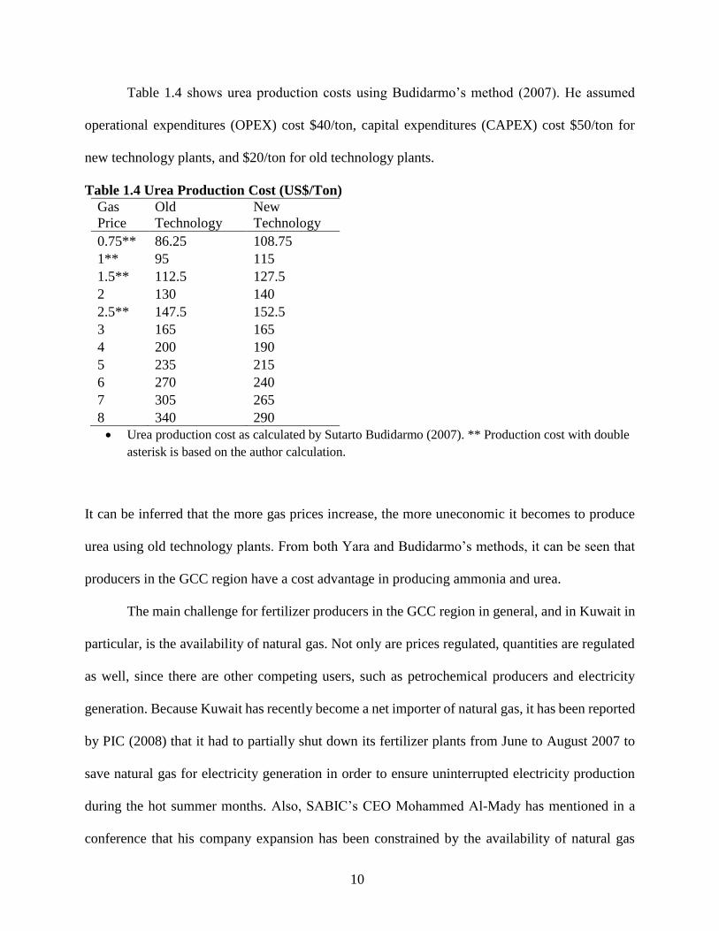
Table 1.4 shows urea production costs using Budidarmo’s method (2007). He assumed
operational expenditures (OPEX) cost $40/ton, capital expenditures (CAPEX) cost $50/ton for
new technology plants, and $20/ton for old technology plants.
Table 1.4 Urea Production Cost (US$/Ton)
Gas
Price
Old
Technology
New
Technology
0.75** 86.25 108.75
1** 95 115
1.5** 112.5 127.5
2 130 140
2.5** 147.5 152.5
3 165 165
4 200 190
5 235 215
6 270 240
7 305 265
8 340 290
Urea production cost as calculated by Sutarto Budidarmo (2007). ** Production cost with double
asterisk is based on the author calculation.
It can be inferred that the more gas prices increase, the more uneconomic it becomes to produce
urea using old technology plants. From both Yara and Budidarmo’s methods, it can be seen that
producers in the GCC region have a cost advantage in producing ammonia and urea.
The main challenge for fertilizer producers in the GCC region in general, and in Kuwait in
particular, is the availability of natural gas. Not only are prices regulated, quantities are regulated
as well, since there are other competing users, such as petrochemical producers and electricity
generation. Because Kuwait has recently become a net importer of natural gas, it has been reported
by PIC (2008) that it had to partially shut down its fertilizer plants from June to August 2007 to
save natural gas for electricity generation in order to ensure uninterrupted electricity production
during the hot summer months. Also, SABIC’s CEO Mohammed Al-Mady has mentioned in a
conference that his company expansion has been constrained by the availability of natural gas

11
supply (Alriyadh, 2014). Another concern for the GCC producers is how long the governments in
the GCC region can keep natural gas prices not only below the international market prices, but
even below production costs, specifically in Saudi Arabia. The main reason Saudi Arabia kept the
low natural gas price of $0.75/MMBTU until 2015 is that the petrochemical companies provide
high quality employment opportunities for citizens, which helps reduce the unemployment rate.
Another possible reason is that the Saudi government owns shares in many petrochemical
companies either directly or indirectly, and hence a portion of their profits go to the Saudi
government.
I estimate the subsidies’ size using the price-gap method because I found that it is the most
straightforward method to estimate governmental support for the fertilizer manufacturers in the
GCC region as compared to international prices. The method was established by Corden (1957).
The method has been used widely in the literature (Liu and Li, 2011; Wang and Lin, 2014; Hong
et al., 2013; Lin and Jiang, 2011; Hua et al., 2012). However, most scholars used it to estimate
subsidy size on a country level or a consumer level. In this paper, I show that this method can be
used on a corporate/firm level. Subsidy size is estimated using the price gap method by first
calculating the difference between end-user price and a reference price.
PG = 𝑃𝑟 − 𝑃𝑠 (1)
PG is the price gap, 𝑃𝑟 is the reference price, and 𝑃𝑠 is the supported or subsidized price. One of
the main criticisms of the price gap approach is the determination of the reference price. To avoid
this criticism in this paper, I will incorporate all the international natural gas prices as reported by
British petroleum (2014) in my analysis. 𝑃𝑠 will be the natural gas prices for the GCC producers,
as in Table 1.1. By combining the price gap and Yara’s method for calculating fertilizer production
cost, I calculate subsidy size as below:

12
Subsidy size = (PG× gas consumption ×𝑄𝐴) + (PG × additional process gas × 𝑄𝑈) (2)
Where 𝑄𝐴 stands for quantity produced of ammonia and 𝑄𝑈 quantity produced of urea. Gas
consumption is the required quantity of natural gas for ammonia production (36 MMBTU natural
gas/tonne ammonia). Additional process gas represents the additional quantity of natural gas
required for urea production (5.8 MMBTU).
The petrochemical industry in the GCC region in general and fertilizer manufacturers in
specific are highly subsidized. The subsidy rate (PG/𝑃𝑟) for SAFCO reached as low as 67% using
Canada (Alberta) international price as a reference price in 2012 and as high as 96% using OECD
as a reference price in 2011, 2012, 2013, and using Japan CIF as a reference price in 2012. For
QAFCO, I assumed the maximum price, $1 MMBTU, and the subsidy rate is as low as 61%
compared with Canada (Alberta) in 2002 and as high as 95% compared with OECD in 2011. For
GPIC, the subsidy rate reached its lowest level compared with Canada (Alberta) when the Bahraini
government increased natural gas prices to $2.25 MMBTU in 2012 and its highest level at 92%
compared with OECD measure. I assume that PIC is charged at the gas ceiling price, $2.50
MMBTU, from 2009–2013, which resulted in no subsidy in 2012 compared with Canada’s
measure. However, if the price was lower than $2.27, which may be true, there would be a subsidy;
but I prefer in this paper to follow the extreme case. However, the subsidy rate reached its peak
point in 1998 compared with Japan CIF price at 90%. In general, the subsidy rate for the fertilizer
industry within the timeframe of the study has been well above 50%, which reflects the large
subsidies. Furthermore, subsidy sizes for these companies reached billions of dollars.
1.5 Model
Hypothesized effects of a per-unit input subsidy on output and profit of a competitive
nitrogen fertilizer firm that uses the inputs (natural gas and labor) to produce an intermediate

13
product (ammonia) that is used in the production of the final product (urea). The excess supply of
ammonia is sold in a competitive market along with the final product (urea).
Let the firm’s objective function be defined as:
max(𝑋) 𝜋 = 𝑝1𝑞1 + 𝑝2𝑞2 − (𝑔 − 𝑠)𝑋 − 𝑤𝐿 − 𝐹𝐶 (3)
where 𝜋 is profit, 𝑝1 is the price of ammonia, 𝑞1 is the excess quantity of ammonia that is offered
for sale, 𝑝2 is the price of urea, 𝑞2 is the quantity sold of urea, 𝑔 is the price of subsidized natural
gas input per MMBTU, 𝑋 is the quantity of natural gas used in ammonia and urea production, 𝑠 is
the per-unit subsidy, 𝑤 is the wage of labor, 𝐿 is quantity of labor, and 𝐹𝐶 is fixed costs.
Let the firm’s production functions for the intermediate (ammonia) and final products (urea) be
defined as:
𝑞1 = 𝑞1(𝑋, 𝐿) (𝜕𝑞1
𝜕𝑋> 0,
𝜕2𝑞1
𝜕𝑋2 < 0; 𝜕𝑞1
𝜕𝐿> 0,
𝜕2𝑞1
𝜕𝐿2 < 0) (4)
𝑞2 = 𝑞2(𝑞1(𝑋, 𝐿)) (𝜕𝑞2
𝜕𝑞1> 0,
𝜕2𝑞2
𝜕𝑞12 < 0) (5)
Production of both products is subject to diminishing marginal products.
Since the firm is assumed to be a perfect competitor in both the output and input markets, prices
are exogenous. This is a reasonable assumption for the GCC producers because in 2011 the total
ammonia production capacity of GCC producers reached 8% of world production capacity, and in
terms of urea it represented 10% of the world’s total production capacity (Markey, 2011). Thus,
the GCC producers can not affect the prevailing international output prices. Moreover, the firms
can not affect natural gas price because natural gas price is regulated by local authority. Hence,
the model contains five endogenous variables (𝜋, 𝑞1, 𝑞2, 𝑋, 𝐿) and six exogenous variables
(𝑝1, 𝑝2, 𝑤, 𝑔, 𝑠, 𝐹𝐶). Since the quantity of ammonia and urea is a function of labor and natural
gas, 𝑄(𝑋, 𝐿), equation (3) can be written as:
𝜋 = 𝑃𝑄(𝑋, 𝐿) + 𝑠𝑋 − 𝑔𝑋 − 𝑤𝐿 − 𝐹𝐶 (6)

14
For the sake of simplicity, I use P to represent output price (either ammonia price or urea price).I
then use comparative static derivatives to obtain the hypothesized impact of the exogenous
variables (output price, wage, natural gas price, and subsidy) on the optimal values of the
endogenous variables. The results of comparative static derivatives are as below (full derivation
of the comparative static derivatives are available in Appendix B).
𝜕�̅�
𝜕𝑔< 0 (a)
In driving the above comparative static results, I assumed a strictly concave production
function (𝑄𝐿𝐿 < 0,𝑄𝑋𝑋 < 0, 𝑎𝑛𝑑 𝑄𝑋𝑋𝑄𝐿𝐿 > 𝑄𝑋𝐿𝑄𝐿𝑋) . The result (a) says that the increase in
natural gas price reduces the quantity demanded of natural gas.
𝜕�̅�
𝜕𝑔< 0 (1b)
In order to sign the comparative static derivative (1b), it is important to know the sign of the cross
partial 𝑄𝐿𝑋, which is the effect of change in natural gas on the marginal productivity of labor.
Hypothetically, if I assume it is positive, an increase in the price of natural gas will decrease the
demand for labor. Thus, (1b) indicates that natural gas and labor are complements. On the other
hand, if I hypothetically assume the sign of 𝑄𝐿𝑋 is negative, I obtain the following comparative
static derivatives:
𝜕�̅�
𝜕𝑔> 0 (2b)
(2b) predicts that an increase in natural gas price increases the demand for labor. Therefore, (2b)
indicates that natural gas and labor are substitutes.
𝜕�̅�
𝜕𝑤< 0 (1c)
Hypothetically, if I assume that the effect of a change in labor on the marginal productivity of
natural gas to be positive, 𝑄𝑋𝐿 > 0. Consequently, (1c) predicts that natural gas demand will

15
decrease in response to an increase in labor wage. Thus, (1c) indicates that natural gas and labor
are complements. However, if I assume the sign for 𝑄𝑋𝐿 is negatives, I obtain the following
comparative static hypothesis.
𝜕�̅�
𝜕𝑤> 0 (2c)
(2c) predicts that natural gas demand will decrease in response to an increase in labor wage. Hence,
(2c) indicates that natural gas and labor are substitutes.
𝜕�̅�
𝜕𝑤< 0 (d)
Comparative static (d) says an increase in wage will reduce the quantity demanded of labor.
The impact of subsidy on the demand for labor and natural gas based on comparative statics results
assuming 𝑄𝐿𝑋 is positive is expressed as follow:
𝜕�̅�
𝜕𝑠> 0 (e)
𝜕�̅�
𝜕𝑠> 0 (f)
Comparative static (e) predicts that an increase in subsidy increases natural gas demand. Also, (f)
indicates that an increase in subsidy increases the demand for labor. Thus, comparative static
derivative (f) satisfies one goal of the energy subsidy in the GCC region, which is to create more
employment opportunities.
The impact of a change in output price (either ammonia price or urea price) on the demand of
natural gas and labor assuming the sign of 𝑄𝐿𝑋 𝑎𝑛𝑑 𝑄𝑋𝐿 is positive can be expressed as below:
𝜕�̅�
𝜕𝑃> 0 (g)
𝜕�̅�
𝜕𝑃> 0 (h)

16
Comparative static (g) indicates that an increase in output price (either urea or ammonia) increases
the demand for natural gas. Moreover, (h) predicts that an increase in output price (either urea or
ammonia) will increase demand for labor.
In order to evaluate the above comparative static hypotheses empirically, I use a translog
specification. The translog specification is a flexible functional form that gives a local second-
order approximation to any arbitrary functional form. The local subsidized natural gas prices are
unaffected by international natural gas prices and international natural gas prices are an important
factor in the nitrogen fertilizer industry. Therefore, I include international natural gas prices in the
model to reveal its impact on local ammonia and urea supply, demand for local natural gas and
labor, and profit of the GCC firms.
ln 𝜋 = 𝑎0 + ∑ 𝑎𝑖 ln 𝑝𝑖 2𝑖=1 + ∑ 𝛽𝑗 ln 𝑤𝑗
2𝑗=1 + 𝑐𝑧 ln 𝑧 + 𝑑𝑠 ln 𝑠 + 𝑒ℎ ln ℎ +
0.5 ∑ ∑ 𝑎𝑖𝑢2𝑢=1
2𝑖=1 ln 𝑝𝑖 ln 𝑝𝑢 + 0.5∑ ∑ 𝛽𝑗𝑙
2𝑙=1 ln𝑤𝑗
2𝑗=1 ln𝑤𝑙 + ∑ ∑ 𝛾𝑖𝑗
2𝑗=1 ln 𝑝𝑖 ln𝑤𝑗
2𝑖=1 +
∑ 𝑎𝑖𝑧 ln 𝑝𝑖 ln 𝑧2𝑖=1 + ∑ 𝛽𝑗𝑧 ln𝑤𝑗 ln 𝑧2
𝑗=1 + ∑ 𝑎𝑖𝑠 ln 𝑝𝑖 ln 𝑠2𝑖=1 + ∑ 𝛽𝑗𝑠 ln𝑤𝑗 ln 𝑠 +2
𝑗=1
∑ 𝑎𝑖ℎ ln 𝑝𝑖 ln ℎ2𝑖=1 + ∑ 𝛽𝑗ℎ ln𝑤𝑗 ln ℎ2
𝑗=1 (7)
Where 𝑝𝑖 and 𝑝𝑢 (𝑖 = 𝑢 = 1 𝑎𝑛𝑑 2) are output prices (ammonia and urea), 𝑤𝑖 and 𝑤𝑙 (𝑖 = 𝑙 =
1 𝑎𝑛𝑑 2) are input prices (natural gas and labor wage), Z is the fixed factor, s is the subsidy, h is
the international natural gas price.
First order differentiation of the profit function with respect to output prices yields the output share
equation:
𝑆𝑖 = 𝑎𝑖 + 𝑎𝑖𝑢 ln 𝑝𝑢 +𝛾𝑖𝑗 ln𝑤𝑗 +𝑎𝑖𝑧 ln 𝑧 + 𝑎𝑖𝑠 ln 𝑠 + 𝑎𝑖ℎ ln ℎ (8)
By differentiating equation (5) with respect to input prices, it results in the unrestricted input share
equation:
𝑆𝑗 = 𝛽𝑗 + 𝛽𝑗𝑙 ln𝑤𝑙 +𝛾𝑖𝑗 ln 𝑝𝑖 + 𝛽𝑗𝑧 ln 𝑧 + 𝛽𝑗𝑠 ln 𝑠 + 𝛽𝑗ℎ ln ℎ (9)

17
1.6 Estimation and Results
Since local natural gas prices are almost fixed and do not vary across years for most of the
observations, I use the real natural gas prices instead of the nominal natural gas prices to allow
some variation in the data. The real natural gas prices are calculated using the U.S. CPI since the
local natural gas prices are valued using dollars. Another issue is the selection of subsidy measure.
Because the total value of the subsidy can be calculated using six different international natural
gas prices as discussed earlier in the paper, I have selected the subsidy calculated using Japan CIF
as the sample of the study due to the fact that these nitrogen fertilizer firms operate in Asia. The
Asian market is the largest market for the GCC fertilizer producers as reported by SAFCO and
QAFCO annual reports. As for international natural gas impact, I chose the U.S. Henry Hub price
as the sample of this study to evaluate its effect on the GCC nitrogen fertilizer industry output
supply, input demand, and profit. I selected Henry Hub as the sample in this paper for three
reasons. First, to avoid possible multicollinearity associated with using the same international gas
price (since I used Japan CIF in subsidy calculation), I needed to use another price than that used
in subsidy calculation. Second, the U.S. market is the second largest market for the GCC nitrogen
fertilizer products and the largest market for GPIC’s urea products, in particular as reported by
GPIC’s annual reports. Third, Henry Hub has a strong reputation to be the most influential
international natural gas price worldwide.
To test for possible endogeneity of international natural gas price and ammonia price, I use
the Hausman specification test since it allows to test whether it is necessary to use instrumental
variable methods instead of a more efficient OLS estimator. The null hypothesis of the test is that
OLS is efficient, hence there is no measurement error. The alternative hypothesis is that the two
stage Least Squares (2SLS) is consistent. The test was performed using SAS software (Proc

18
Model). Results show that I reject the null hypothesis of no measurement error. Thus, an
instrumental variable estimator is used in estimating the system of output-input shares and profit
function equations. I estimate the model using generalized method of moments (GMM). I
implement the GMM method by using the Proc Model procedure in SAS software. The Hansen’s
J test statistics indicates that the instruments are uncorrelated with the disturbance.
Furthermore, since the data is panel data, I added three dummy variables to account for the
fact that the data is a panel data consisting of four firms. For the fixed input, I consider the
accounting value of plant and equipment as the fixed input in this study. For GPIC, I use capital
expenditure on assets as a proxy for the fixed input variable. There were few missing observations
for QAFCO’s fixed input. These missing observations were recovered using a linear trend method
following (Coelli, Rahman, & Thirtle, 2003). Labor price is payments to labor divided by number
of labors. Missing observations for labor price for GPIC, QAFCO, and PIC were recovered using
wage and labor survey and statistics that closely matches fertilizer industry. Table 1.5 shows
descriptive statistics for the key variables of the model.
Table 1.5 Descriptive Statistics of the Model Key Variables Variables Observations Mean Std Dev Minimum Maximum
Ammonia Price 59 284.11 135.52 95.00 515.00
Urea Price 59 254.55 120.74 66.00 475.00
Real Natural Gas
Price
59 1.33 0.58 0.43 2.71
Wage 59 22458.63 21968.31 1335.91 94263.49
Plant & Equipment 59 493476396.00 584516794.00 5035000.00 3500285294.00
Ammonia Share (S1) 59 0.30 0.37 -1.37 1.84
Urea Share (S2) 59 0.96 2.80 -17.03 11.83
Natural Gas Share
(S3)
59 -0.20 0.72 -2.34 4.49
Labor Share (S4) 59 -0.06 2.41 -10.34 14.91
Profit 59 539801852 615750768 -3127161.46 2147469879
*All values in US$
In estimating the model, I dropped the urea share equation to avoid singularity in the variance-
covariance matrix. The instruments I used are chemicals and related product price index, mineral

19
and fuel price index, and OPEC basket price as reported by Saudi Arabian Monterey Agency (the
central bank of Saudi Arabia). Other instruments include third lag prices of both ammonia and
Canada (Albarta) natural gas. The homogeneity and symmetry restrictions were imposed in the
estimation process. Table 1.6 shows the estimated parameters of the model based on GMM
estimator before standard error correction. Table 1.7 shows the parameters estimate after standard
error correction using the Newey-West standard error correction method. Generally, standard error
correction has improved the parameters’ t-ratio. However, the sign of the parameters has not
changed. The Shapiro-Wilk normality test shows that the assumption of normal distribution hold
for the case of the profit function. Also, the 𝑅2 shows that the model explains 80% of the variation
in the profit function of the selected GCC firms.
Table 1.6 Parameter Estimates Based on GMM Estimator
Dependent
Variable Intercept
Ammonia
Price Urea Price
N Gas
Price Wage
Fixed
Input Subsidy Int N Gas
Dummy
Variable
Ammonia
0.103
(0.064)
0.049
(0.129)
0.161
(0.120)
-0.219***
(0.072)
0.009
(0.013)
0.067***
(0.021)
-0.188***
(0.032)
-0.083*
(0.045)
-
Urea 6.577
(0.076)
-0.562***
(0.153)
0.313***
(0.101)
0.088***
(0.031)
0.103**
(0.044)
0.494***
(0.174)
0.462
(0.411)
-
N Gas -0.046
(0.105)
-0.157*
(0.087)
0.064***
(0.017)
-0.019
(0.019)
0.144***
(0.047)
0.101
(0.074)
-
Labor -0.074
(0.122)
-0.161***
(0.035)
-0.150***
(0.049)
0.278***
(0.047)
0.510***
(0.105)
-
Profit
𝑅2
6.594***
(2.010)
0.80
- - - - - - - 3.027***
(0.294)
0.002
(0.654)
0.0001
(0.466)
Note: N Gas is local natural gas and Int N Gas is international natural gas price.
Standard errors are in parenthesis
***Significant at 1%, **significant at 5%, and * significant at 10%.

20
Table 1.7 Parameter Estimates Based on GMM Estimator after Standard Error Correction
Dependent
Variable Intercept
Ammonia
Price Urea Price
N Gas
Price Wage
Fixed
Input Subsidy Int N Gas
Dummy
Variable
Ammonia
0.253***
(0.010)
0.053
(0.056)
0.206***
(0.055)
-0.271***
(0.018)
0.019**
(0.005)
-0.069***
(0.010)
-0.211***
(0.013)
-0.161***
(0.026)
-
Urea 1.536***
(0.012)
-0.561*
(0.561)
0.297*
(0.159)
0.059***
(0.013)
0.191***
(0.040)
0.377**
(0.166)
0.481**
(0.180)
-
N Gas -0.112***
(0.021)
-0.150***
(0.031)
0.124***
(0.015)
-0.020
(0.019)
0.228***
(0.026)
0.298***
(0.061)
-
Labor -0.375***
(0.122)
-0.194***
(0.016)
-0.241***
(0.030)
0.338***
(0.033)
0.665***
(0.073)
-
Profit
𝑅2
-0.302
(0.257)
0.82
- - - - - - - -0.302***
(0.000)
-0.302
(1.038)
-0.302
(1.038)
Note: N Gas is local natural gas and Int N Gas is international natural gas price.
Standard errors are in parenthesis
***Significant at 1%, **significant at 5%, and * significant at 10%.
I then calculated the elasticities using the formulas in Table 1.8. The estimated elasticities along
with their significance level are reported in Table 1.9 and table 1.10 based on the GMM estimator
before and after standard error correction, respectively. It is important to note that standard error
correction has not altered the estimated elasticities sign. However, it has indeed improved the t-
ratio for the estimated elasticities.

21
Table 1.8 Elasticity Formula
Elasticity Expression
Output Own Price Supply Elasticity 𝑎𝑖𝑖+𝑆𝑖
𝑆𝑖 + 1
Cross Output Price Supply Elasticity 𝑎𝑖𝑢
𝑆𝑖+ 𝑆𝑢
Supply Elasticity wrt Input Price −𝛽𝑖𝑙
𝑆𝑖− 𝑆𝑙
Supply Elasticity wrt Fixed Factor 𝑐𝑧 + 𝑎𝑖𝑧 ln 𝑝𝑖 + 𝑎𝑢𝑧 ln 𝑝𝑢 + 𝛽𝑗𝑧 ln𝑤𝑗
+ 𝛽𝑙𝑧 ln𝑤𝑙 + [𝑎𝑖𝑧
𝑠𝑖]
Supply Elasticity wrt Subsidy 𝑑𝑠 + 𝑎𝑖𝑠 ln 𝑝𝑖 + 𝑎𝑢𝑠 ln 𝑝𝑢 + 𝛽𝑗𝑠 ln𝑤𝑗
+ 𝛽𝑙𝑠 ln𝑤𝑙 + [𝑎𝑖𝑠
𝑠𝑖]
Supply Elasticity wrt Subsidy Int NG 𝑒ℎ + 𝑎𝑖ℎ ln 𝑝𝑖 + 𝑎𝑢ℎ ln 𝑝𝑢 + 𝛽𝑗ℎ ln𝑤𝑗
+ 𝛽𝑙ℎ ln𝑤𝑙 + [𝑎𝑖ℎ
𝑠𝑖]
Input Own Price Demand Elasticity −𝛽𝑗𝑗
𝑆𝑗− 𝑆𝑗 − 1
Cross Price Elasticity of Demand for Input −𝛽𝑗𝑙
𝑆𝑗− 𝑆𝑙
Elasticity of demand for Input wrt output
price
−𝛾𝑗𝑖
𝑆𝑗+ 𝑆𝑖
Elasticity of Demand for Input wrt Fixed
Factor 𝑐𝑧 + 𝑎𝑖𝑧 ln 𝑝𝑖 + 𝑎𝑢𝑧 ln 𝑝𝑢 + 𝛽𝑗𝑧 ln𝑤𝑗
+ 𝛽𝑙𝑧 ln𝑤𝑙 − [𝛽𝑗𝑧
𝑠𝑗]
Elasticity of Demand for Input wrt Subsidy 𝑑𝑠 + 𝑎𝑖𝑠 ln 𝑝𝑖 + 𝑎𝑢𝑠 ln 𝑝𝑢 + 𝛽𝑗𝑠 ln𝑤𝑗
+ 𝛽𝑙𝑠 ln𝑤𝑙 − [𝛽𝑗𝑠
𝑠𝑗]
Elasticity of Demand for Input wrt Int NG 𝑒ℎ + 𝑎𝑖ℎ ln 𝑝𝑖 + 𝑎𝑢ℎ ln 𝑝𝑢 + 𝛽𝑗ℎ ln𝑤𝑗
+ 𝛽𝑙ℎ ln𝑤𝑙 − [𝛽𝑗ℎ
𝑠𝑗]

22
Table 1.9 Estimated Elasticities Evaluated at the Mean Data Points Based on GMM
Ammonia
Price
Urea
Price
N Gas
Price Wage
Fixed
Input Subsidy Int N Gas
Ammonia 0.269***
(0.099)
1.498***
(0.398)
0.931***
(0.242)
0.029
(0.044)
0.426***
(0.107)
-0.017
(0.158)
0.022
(0.260)
Urea 0.468***
(0.125)
1.356***
(0.153)
-0.125
(0.105)
-0.034
(0.032)
0.311***
(0.087)
1.123***
(0.198)
0.780*
(0.404)
N Gas -0.790**
(0.202)
2.515***
(0.502)
-1.582***
(0.436)
0.377***
(0.084)
0.107
(0.116)
1.325***
(0.305)
0.802*
(0.424)
Labor 0.453*
(0.227)
2.472***
(0.526)
1.294***
(0.287)
-3.700***
(0.590)
-2.374***
(0.821)
5.368***
(0.829)
9.026***
(1.719)
Profit -0.264
(0.457)
1.329***
(0.436)
0.133
(0.239)
-0.198***
(0.064)
0.135**
(0.057)
0.825***
(0.139)
0.657***
(0.140)
***Significant at 1%, **significant at 5%, and * significant at 10%.
Table 1.10 Estimated Elasticities Evaluated at the Mean Data Points after Standard Error
Correction
Ammonia
Price
Urea
Price
N Gas
Price Wage
Fixed
Input Subsidy Int N Gas
Ammonia 0.272***
(0.043)
1.644***
(0.184)
1.103***
(0.061)
0.019
(0.016)
0.463***
(0.058)
-0.041
(0.059)
-0.175
(0.137)
Urea 0.515***
(0.090)
1.358***
(0.276)
-0.108
(0.165)
-0.003
(0.014)
0.433***
(0.062)
1.055***
(0.195)
0.861***
(0.159)
N Gas -1.047***
(0.202)
2.435***
(0.149)
-1.546***
(0.155)
0.677***
(0.076)
0.134**
(0.054)
1.796***
(0.139)
1.843***
(0.295)
Labor 0.504***
(0.080)
1.960***
(0220)
2.326***
(0.260)
-4.270***
(0.277)
-3.885***
(0.488)
6.436***
(0.549)
11.728***
(1.217)
Profit -0.172
(0.161)
1.300***
(0.131)
0.076
(0.073)
-0.204***
(0.022)
0.123**
(0.021)
0.904***
(0.053)
0.819***
(0.059)
***Significant at 1%, **significant at 5%, and * significant at 10%.
Before discussing the estimated elasticities, it is important to note that beside the symmetry
and homogeneity that were imposed in the estimation, monotonicity and convexity are additional
properties of a profit function that cannot be satisfied globally with the translog function. However,
they may hold at specific data points used in estimating the function (Fulginiti and Perrin, 1990).
Monotonicity is violated if the estimated output shares are negative or the estimated input shares
are positive. Thus, monotonicity is satisfied in this study at the average data point. On the other
hand, convexity is violated if own output price elasticity has a negative sign or own input price
elasticity has a positive sign. The estimated elasticities in table 1.9 and table 1.10 show that all the
own input and output price elasticities have the correct sign at the average data point, and hence

23
convexity is not violated. The cross supply elasticities are positive, indicating a complementary
relationship between ammonia and urea. Before standard error correction, the elasticity of
ammonia supply in response to a general increase in ammonia and urea prices is 1.767. Similarly,
the elasticity of urea supply in response to a general increase in both ammonia and urea prices is
almost 1.824. After standard error correction these elasticities are 1.916 and 1.873, respectively.
This indicates that a general increase in output prices, holding the impact of input prices constant,
would cause an elastic response of aggregate output. Ammonia supply elasticity, with respect to
domestic natural gas price, is positive indicating that natural gas is inferior input in ammonia
supply. This case is true due to both cheap local natural gas prices and because the GCC producers
produce urea and the excess (unused) ammonia is offered for sale. Moreover, the results show that
labor price does not affect ammonia and urea supply.
Own price input demand elasticity for local natural gas and labor are -1.582 and -3.700 (-
1.546 and -4.270 after standard error correction). Thus, a one percent increase in local natural gas
price decreases natural gas consumption approximately by 1.6 percent. As a result, I accept the
result of comparative static hypothesis (a), which indicated that the increase in the price of natural
gas decreases natural gas consumption. Also, a one percent increase in the wage of labor decreases
the quantity demanded of labor by more than 3 percent. As a result, I accept the result of hypothesis
(d) since it indicted that the increase in wage decreases the quantity demanded of labor.
Furthermore, Castro and Teixeira (2011) stated that elastic demands are consistent with an
oligopolized sector, which may be true for the GCC producers since there are few producers in the
GCC region, as shown in Table 1.A1 in Appendix A. All input cross price elasticities are positive,
meaning that natural gas and labor are substitutes. Thus, I accept hypotheses (2b) and (2c).
Consequently, I reject hypotheses (1b) and (1c). The impact of natural gas demand to a general

24
combined increase in domestic natural gas price and labor wages is -1.205, compared with -2.406
for labor demand (-0.869 and -1.944 after standard error correction). Holding the impact of output
prices constant, an increase in input prices would impact natural gas consumption less than labor
use.
The demand for inputs are elastic with respect to the urea price, revealing a higher degree
of responsiveness of labor and natural gas to changes in urea price. Therefore, I accept hypotheses
(g) and (h) for the case of urea price since an increase in urea price increases the demand for both
natural gas and labor. The reason labor has a very high elastic response with respect to the urea
price is because some wage observations are annual aggregate salaries and include bonuses.
Bonuses according to the GCC firms are given at the end of the year after evaluating the prevailing
macroeconomic conditions and end of the year’s profit of the firm (or its mother company in case
of SAFCO). Profit of the GCC nitrogen fertilizer firms are highly linked to changes in quantity
sold of urea and urea prices; this is the reason that the average urea shares, as shown in Table 1.1,
is 0.96. Moreover, SABIC, the owner of SAFCO, has given and demanded all its affiliates
(including SAFCO) to give all the employees a bonus, equivalent to a 4 month salary, in 2007 and
in 2011, and a 3 month salary in 2009, 2010, 2012, and 2013. Conversely, during the great
recession in 2008, SABIC had suspended its employees’ promotions and limited bonuses to a 2
month salary. In 2014, the company paid an equivalent to 2.85 month salary. The other companies
in the sample of this study pay bonuses as well, but there is no precise information on the bonus
disbursement policy.
The estimated elasticities predict that an increase in ammonia price has an adverse effect
on natural gas demand. Thus, I reject hypothesis (g) for the case of ammonia price. This is because
ammonia production requires less quantity of natural gas than urea and increases in ammonia price

25
would encourage the GCC producers to offer more ammonia for sale. This will result in a reduction
in the use of natural gas. Also, ammonia price has a positive inelastic effect on the demand for
labor. Thus, I accept hypothesis (h) for the case of ammonia price since an increase in ammonia
price increases the demand for labor. Additionally, the fixed factor has inelastic positive effect on
ammonia supply, urea supply, and profit. After standard error correction, the results show that the
fixed factor positively affects the demand for natural gas. However, the fixed factor has an elastic
negative effect on labor demand. This has an important policy implication. This implies that the
GCC producers are using advanced technology in their plants and equipment, which reduces the
demand for labor.
The subsidy is statistically significant and it has a positive elastic effect on natural gas
demand. Thus, I accept hypothesis (e) since an increase in subsidy increases natural gas demand.
The results show that subsidy does not affect ammonia supply. This indicates that the subsidy is
directed toward urea production, and the leftover ammonia is supplied to the market. Moreover,
the subsidy has a positive inelastic and significant at the one percent level effect with respect to
profit. This shows that a one percent decrease in subsidy decreases profit by 0.825 percent (0.904
percent after standard error correction). This result confirms the GCC nitrogen fertilizer
executives’ claim that changes in subsidy would adversely affect the profitability of the nitrogen
fertilizer producers. Also, a statistically significant positive impact of subsidy on labor demand
shows that the subsidy program in the GCC region has achieved one of its governmental goals in
terms of creating more employment opportunity. Therefore, a one percent increase in subsidy
increases demand for labor by 5.368 percent (6.436 percent after standard error correction).
Consequently, I accept hypothesis (f) since an increase in subsidy increases the demand for labor.

26
The impact of international natural gas prices, as measured using the U.S. Henry Hub
international gas price, does not affect ammonia supply. Also, the international natural gas price
has a positive statistically significant effect at the ten percent level on urea supply. The
international natural gas price has a positive inelastic effect on domestic natural gas demand. After
standard error correction, the results show that international natural gas price has a positive elastic
effect on domestic natural gas demand. QAFCO, as shown in its financial statement, sells excess
(unused) natural gas. Hence, the increase in international natural gas prices would cause QAFCO
to demand more natural gas, and then sell it after it satisfies its needs to produce both ammonia
and urea. SAFCO has the ability to sell its excess shares of subsidized natural gas to its other
SABIC’s affiliates; however, there is no information on SAFCO and the other firms, other than
QAFCO in the sample of this study that they can sell the excess natural gas. In addition, the
international natural gas price has a positive inelastic impact on the profitability of the GCC firms.
Increases in international natural gas prices mean automatically that nitrogen fertilizer prices will
increase, which would mean that the profit of the GCC firm will increase as a result. The largest
impact of international natural gas price is observed on labor demand. Labor demand is highly
elastic with respect to international natural gas price. Thus, a one percent increase in international
natural gas price increases labor demand by 9.026 percent (11.728 percent after standard error
correction). Urea Price is elastic with respect to profit indicating that the profitability of the GCC
producers is highly responsive to changes in urea price. The results show that a one percent
increase in urea price increases profit by aprroximatly1.3 percent.

27
1.7 Conclusion
This paper analyzed the impact of energy subsidies on nitrogen fertilizer producers in the
GCC region, which export the majority of their output. I estimated ammonia production cost per
ton using Yara’s method and found the cost of production in Saudi Arabia to be $53, in Qatar and
the UAE it is approximately $64, in Bahrain prior to the 2012 increase in natural gas is $80, in
Oman after the 2013 increase in natural gas price is $98, and $116 assuming PIC was charged
$2.50. Similarly, production cost for urea per ton is $57, $63.16, $76.20, 89.24, and $102.28 for
the mentioned countries/firms respectively. In addition, I showed urea production cost per ton
using Budidarmo’s method is $86.25, $95, $112.50, $130, and $147.50 assuming the use of old
technology plants and $108.75, $115, $127.50, $140,and $152.50 assuming the use of new
technology plants. SAFCO, QAFCO, GPIC, and PIC were chosen as the focus of this study as they
disclose their financial statements. Then, I estimated subsidy size using the price gap approach.
The subsidy was estimated to vary from millions to billions of dollars compared with other
international natural gas prices as reported by British Petroleum, except PIC in 2012. I then
developed a multiple input-output translog model to evaluate the impact of energy subsidy and
international gas prices on output supply, input demand, and profit of the GCC firms. The results
based on the GMM estimator show that output supply, input demand, and profits are elastic and
statistically significant at the one percent level with respect to urea price indicating a high degree
of responsiveness to changes in urea selling prices. Also, the results show that local natural gas is
an inferior input in ammonia production and a normal input in urea production. Moreover, the
results show that ammonia and urea are complements. The fixed inputs, as measured by the value
of plant and equipment, has a negative elastic effect on labor demand. This implies that the GCC
producers are using a production technology that requires less labor. Also, the fixed input has a

28
positive inelastic effect on ammonia supply, urea supply, and profit of the GCC fertilizer
producers.
Energy subsidy has a positive inelastic influence on domestic natural gas demand due to
the fact that the producers in the GCC region have a predetermined quantity of subsidized natural
gas input. In addition, energy subsidy has an elastic positive effect on urea supply and labor
demand. Moreover, despite the distorting impact of subsidies on output supply and input demand,
the study shows that the GCC executives’ claim that changes in energy subsidies would adversely
impact their profit is a valid claim. The results show that subsidy has an inelastic significant
positive effect on profit. Thus, a one percent decrease in subsidy decreases profit by 0.62 percent
and vice versa. Therefore, the study concluded that the energy subsidies in the GCC region have
achieved one of its governmental purposes in terms of creating more employment opportunities
and increasing the competitiveness of the GCC firms in international marketplace by reducing
their production costs and increasing their profitability. On the other hand, international natural
gas prices as measured by the U.S. Henry Hub international natural gas price, as a sample for this
paper, showed a positive inelastic impact on urea supply, local natural gas demand, and profit of
the GCC firms. The study recommends for future research to conduct a cost benefit analysis for
the GCC governments considering the opportunity cost of selling natural gas in international
markets, instead of selling it at the local market, bearing in mind that the GCC governments receive
part of the chemical and petrochemical corporates’ profit.

29
Chapter2
Economies of Scale, Technical Change, and Total Factor
Productivity Growth of the Saudi Electricity Sector.
2.1 Introduction
The electric sector in Saudi Arabia is fully regulated by the government. In 2000, the
council of ministers issued a royal decree to restructure the electric sector that used to be fully
owned and managed by the government. This resulted in the consolidation of unified electricity
firms working in eastern, central, western, and southern regions in addition to ten companies
working in the northern region into a vertically integrated utility company. Furthermore, the
decree stipulated the listing of the company as Saudi Electricity Company (SEC) in the Saudi stock
market. Currently, 74.3 percent of company stock is owned by the government, 6.92 percent is
owned by the Saudi Arabian oil company (ARAMCO), and the remaining stocks are owned by the
public. As stated in the company’s website, the company supplies over 75 percent of the generation
capacity and maintains a monopoly position in the transmission and distribution of electricity. The
company purchases energy to cover the deficit in electricity generation from the water and
electricity company, desalination plants, and other producers. Furthermore, since the establishment
of the SEC, the company has enjoyed much governmental support and privileges such as interest
free loans, loan payment deferral, and waiver of dividends on the government’s shareholding.
The mission of the SEC is to optimize its resources in generating electricity to meet the
increased demand for electricity from various users such as residential, industrial, and commercial.
The company’s aim is to reduce the cost of electricity production. Thus, it is very important to
conduct an empirical examination of the company’s mission and aim statement by examining how

30
SEC uses its input efficiently in delivering its output to the final users. To my knowledge, there
has not been a study that examines economic productivity and efficiency in the Saudi electricity
sector. Therefore, the purpose of this paper is to examine the presence of economies of scale,
technical change, and total factor productivity growth. Also, the paper tries to extend the existing
literature about the decomposition of total factor productivity growth (TFP) by deriving an
equation that takes into account the impact of network characteristics in TFP decomposition. The
other objective of the paper is to inform the decision makers in the SEC about the optimal scale of
operation.
2.2 Literature Review
The studies that have analyzed the electricity industries can be generally classified into two
groups with regard to their empirical methodology. The first group employs a non-parametric
approach that usually uses the data envelopment analysis (DEA) and the second group employs a
parametric approach mostly using a stochastic frontier approach, a cost function, a production
function and a distance function.
(Huang et al., 2010) used a stochastic meta frontier approach to estimate the cost efficiency
of Taiwan’s electricity distribution units. Their results show that the high circuit density group is
more efficient than low circuit density group due to the impact of network characteristics in
determining the efficiency for the electricity distribution industry. Also, they find that the current
scale of distribution is smaller than the optimal scale. Using an input distance function (Subal et
al., 2015) analyzed Norwegian electricity distribution companies. They concluded that the smaller
companies achieved economies of scale and some of them are technically efficient while they
could not find evidence of economies of scale among larger firms. Also, the authors found that
technical progress in the industry had no relationship between technical change and firm size. As

31
for studies in the U.S. electric sector, (Christensen and Greene, 1976) found evidence of scale
economics in the U.S. electric power generation in 1955, (Atkinson and Halvorsen , 1984) found
the range of estimates of scale economies using total shadow cost in range of 54.0 percent to -1.7
percent, and (Okunade, 1993) found the average scale economies of 0.26 in a sample of privately
regulated private steam-electric utilities in East-North-Central U.S.. (Gao et al., 2013) studied the
US electric power industry and found that on average the industry had its highest TFP growth rate
in 2005 and 2008 and negative TFP growth rate in 2002 and 2007. (Andrikopulos and Vlachou,
1995) found evidence of economies of scale and the average TFP growth rate is 0.017 percent in
the Greek public electric power industry. (Efthymoglou and Vlachou, 1989) estimated that the TFP
of the integrated Greek power system increase at an average annual growth rate of 1.76 percent.
(Filippini, 1998) used a translog cost function approach on a sample of Swiss municipal utilities.
He concluded that the Swiss utilities operate with economies of output density, economies of
customer density, and economies of scale. (Roberts, 1986) used a tronslog cost function approach
and rejected the hypothesis of no economies of output density and customer density at the one
percent level. Additionally, he rejected the hypotheses of no economies of size at the five percent
level. (Tovar et al., 2011) analyzed Brazilian electricity distribution industry using a stochastic
translogarithmic distance function. The results show a positive TFP with an annual growth of 0.9
percent during 1998-2005 and the average technical change growth is estimated to be 4.9 percent.
(Goto and Sueyoshi, 2009) found evidence of economies of scale, negative technical change (due
to large investment cost), and a negative TFP growth in the Japanese electricity distribution
industry. The study also indicated that the network characteristics (load factor, customer density,
and underground ratio of lines) influence the cost of distribution. (See and Coelli, 2013) found the
average TFP growth in the Malaysian electricity generation industry of 0.5 percent, 0.94 percent,

32
and 2.34 percent using Malmquist method, Törnqvist method, and stochastic frontier analysis,
respectively. The authors attributed the differences because different methods use different explicit
or implicit cost and revenue share to weight inputs and output variables components. (Arcos and
de Toledo, 2009) concluded that the Spanish electricity utility industry exhibit diseconomy of
scale. (Akkemik, 2009) found that the technical change in the Turkish electricity generation sector
is energy using and labor and capital saving. Also, the results showed presence of economies of
scale and a general trend for technological progress to deteriorate. (Oh, 2015) analyzed Korean
fossil-fuel generation companies and found evidence of economies of scale, technical
deterioration, average scale component of 1.459 percent, and, on average, a negative TFP growth
rate of -0.697 percent. (Burney, 1998) estimated a translog variable cost function using a time
series data on Kuwait electricity generation sector. The author found evidence supporting the
presence of diseconomy of scale in electricity generation in Kuwait. (Hisnanicka and Kymnb,
1999) stressed the importance of additional research to investigate the impact of scale economies
on productive behavior.
Studies on the electric sector that used non-parametric approach are many. For example,
(Lam and Shiu, 2004) China’s thermal power generation using a DEA approach. They found the
average TFP growth rate is 2.1 percent. (Abbott, 2006) analyzed the Australian electricity supply
industry using DEA approach and found an average technical progress growth rate of 1.8 percent,
and a TFP average annual growth rate of 2.5 percent. (Çelen, 2013) estimated the mean TFP
change of 1.033 percent in Turkish electricity distribution companies. See and Coelli (2014) use
Törnqvist index to estimate TFP growth of Tenaga Nasional Berhad in Malaysia. The study found
a TFP growth of 1.19 percent prior to the company’s corporatization, 5.73 percent after the
company corporatization, and 0.36 for the full period of study.

33
To my knowledge, this is the first paper that analyzes economies of scale, technical change,
and TFP growth of the Saudi electricity sector. Also, this is the first study that includes network
characteristics in TFP growth decomposition.
2.3 Methodology and Data
2.3.1 Theoretical Model
The model that will be used in this paper is the same model derived by (Oh, 2015).
However, this paper will improve Oh’s model by incorporating network characteristic into the
decomposition of TFP. Thus, the approach is a dual approach that uses a cost function. The model
assumes that firms minimize costs and that factor markets are competitive. The cost function is
represented as:
C= C(w, y, N, t) (1)
where C is the total cost, w represents input prices, y is firm’s output, N is network characteristics
such as customer density, length of transmission and distribution line, etc. and t is a time trend
variable.
By taking the total differential, equation (1) becomes
𝑑𝑙𝑛𝐶 = ∑𝜕𝑙𝑛 𝐶
𝜕𝑙𝑛𝑤𝑖𝑖 𝑑𝑙𝑛𝑤𝑖 +
𝜕𝑙𝑛 𝐶
𝜕𝑙𝑛𝑦𝑑𝑙𝑛𝑦 +
𝜕𝑙𝑛𝐶
𝜕𝑙𝑛𝑁𝑑𝑙𝑛𝑁 +
𝜕𝑙𝑛𝐶
𝜕𝑡𝑑𝑡 (2)
By applying Shephard’s lemma, we obtain the following cost share equation:
𝜕𝑙𝑛𝐶
𝜕𝑙𝑛𝑤𝑖=
𝑤𝑖𝑥𝑖
𝐶= 𝑆𝑖 (3)
𝑆𝑖 denotes input cost share. Inserting equation (3) into (2) yields the following

34
𝑑𝑙𝑛𝐶
𝑑𝑡= ∑ 𝑆𝑖𝑖
𝑑𝑙𝑛𝑤𝑖
𝑑𝑡+
𝜕𝑙𝑛𝐶
𝜕𝑙𝑛𝑦
𝑑𝑙𝑛𝑦
𝑑𝑡+
𝜕𝑙𝑛𝐶
𝜕𝑙𝑛𝑁
𝑑𝑙𝑛𝑁
𝑑𝑡+
𝜕𝑙𝑛𝐶
𝜕𝑡 (4)
The above logarithmic time derivatives, which denote rate of change, can be expressed as:
�̇� = ∑ 𝑆𝑖𝑖 𝑤𝑖̇ +𝜕𝑙𝑛𝐶
𝜕𝑙𝑛𝑦�̇� +
𝜕𝑙𝑛𝐶
𝜕𝑙𝑛𝑁�̇� +
𝜕𝑙𝑛𝐶
𝜕𝑡 (5)
Since the logarithmic time derivatives of cost2 and the Divisia index of total factor productivity
growth(𝑇𝐹�̇�) are expressed as:
�̇� = ∑ 𝑆𝑖𝑖 𝑋𝑖̇ + ∑ 𝑆𝑖𝑖 𝑤𝑖̇ (6)
𝑇�̇�𝑃 = �̇� − ∑ 𝑆𝑖𝑖 𝑋𝑖̇ (7)
By inserting equation (6) into (7), we obtain
𝑇�̇�𝑃 = �̇� − (�̇� − ∑ 𝑆𝑖𝑖 𝑤𝑖̇ ) (8)
where �̇� is the growth rate of output. Then by inserting equation (5) into equation (8), we obtain
the final decomposition of 𝑇𝐹�̇� growth that takes into account the impact of network
charactaristics as below:
𝑇�̇�𝑃 = �̇� − (∑ 𝑆𝑖𝑖 𝑤𝑖̇ +𝜕𝑙𝑛𝐶
𝜕𝑙𝑛𝑦�̇� +
𝜕𝑙𝑛𝐶
𝜕𝑙𝑛𝑁�̇� +
𝜕𝑙𝑛𝐶
𝜕𝑡− ∑ 𝑆𝑖𝑖 𝑤𝑖̇ ) (9)
𝑇�̇�𝑃 = (1 −𝜕𝑙𝑛𝐶
𝜕𝑙𝑛𝑦) �̇� + (−
𝜕𝑙𝑛𝐶
𝜕𝑙𝑛𝑁�̇�) + (−
𝜕𝑙𝑛𝐶
𝜕𝑡) (10)
𝑇�̇�𝑃 = 𝑆𝐶 + (−휀𝑁�̇�) + 𝑇𝐶 (11)
2 For further details regarding the derivation of the logarithmic time derivatives of cost equation (6), please refer to Oh (2015).

35
where SC denotes scale component. 휀𝑁 is the elasticity of total cost with respect to the network
variable and �̇� is the growth rate in the network variable. TC is the technical change.
Some authors who did not include network characteristics in their analysis, such as (Akkemik
,2009) and (Oh, 2015) have defined economies of scale as the elasticity of total cost with respect
to output, 𝜕𝑙𝑛𝐶
𝜕𝑙𝑛𝑦 . On the other hand, (Christensen and Greene, 1976) have defined economies of
scale as unity minus the elasticity of total cost with respect to output. 1 −𝜕𝑙𝑛𝐶
𝜕𝑙𝑛𝑦.
The scale components shows how a firm adjusts its size to approach or deviate from the optimal
size. As mentioned by Oh, if a firm is operating under the economies of scale (or economies of
output density for authors who include network characteristics) and increasing its size, then the
scale component is positive. Also, a positive scale component can occur if a firm is operating under
diseconomies of scale and decreasing its firm size. Conversely, a negative scale component
indicates that the firm is deviating far from the optimal size.
The technical change term, which equals the negative of the elasticity of total cost with respect to
time, shows the reduction in firm’s cost over time.
Therefore, the proposed total factor productivity growth in this paper equals the summation of
scale component, the negative of the elasticity of network variables times their growth, and
technical change.
2.3.2 Econometric Model
This paper will use translog cost function approach since it has been widely used in the
literature to estimate empirically the cost function in the electricity industry, for example
(Akkemik, 2009) and (Filippini, 1998). The model is written as:

36
𝑙𝑛𝐶 = 𝑎𝑐 + 𝑎𝑦𝑙𝑛𝑦 +1
2 𝑎𝑦𝑦(𝑙𝑛𝑦)2 + 𝑎𝑡𝑡 +
1
2 𝑎𝑡𝑡𝑡
2 + 𝑎𝑦𝑡(ln𝑦)𝑡 + ∑ 𝛿𝑖𝑖 𝑙𝑛𝑃𝑖 +
1
2∑ ∑ 𝛾𝑖𝑗𝑙𝑛𝑃𝑖𝑗𝑖 𝑙𝑛𝑃𝑗 + ∑ 𝛾𝑖𝑦𝑙𝑛𝑃𝑖 𝑙𝑛𝑦𝑖 + ∑ 𝛾𝑖𝑡𝑖 𝑙𝑛𝑃𝑖 𝑡 + 𝜑𝑖𝑁𝑖 (12)
Where C denotes total cost, y is output, t is a time trend variable, 𝑃𝑖 and 𝑃𝑗 is the price of the ith
and jth input (𝑓 = 𝑓𝑢𝑒𝑙, 𝑒 = 𝑝𝑢𝑟𝑐ℎ𝑎𝑠𝑒𝑑 𝑒𝑛𝑒𝑟𝑔𝑦, 𝑎𝑛𝑑 𝑘 = 𝑐𝑎𝑝𝑖𝑡𝑎𝑙), and N is a variable
accounting for network characteristics. 𝛼𝑐is the intercept for the cost
function.𝑎𝑡, 𝑎𝑡𝑡, 𝑎𝑦𝑡, 𝛾𝑖𝑗, 𝛾𝑖𝑦, 𝛾𝑖𝑡, 𝛿𝑖 𝑎𝑛𝑑 𝜑𝑖 are parameters to be estimated. The network variable
is specified in a linear way following (Goto and Sueyoshi, 2009). Also, I include a dummy variable
in the model to distinguish the time period prior to SEC incorporation in 2000 from the period
after SEC incorporation.
Homogeneity condition in input prices requires ∑ 𝛿𝑖 = 1,∑ 𝛾𝑖𝑗 = 0,∑ 𝛾𝑦𝑖𝑖𝑖𝑗𝑖 = 0, 𝑎𝑛𝑑 ∑ 𝛾𝑖𝑡𝑖 = 0.
By normalizing total cost and input prices by a chosen input price, we impose the homogeneity
condition. There are many studies in the electricity sector that followed this approach (Filippini,
1998; Huang et al. 2010; Fetz and Filippini, 2010; Oh, 2015). In this paper, I will follow the same
approach. The symmetry condition (𝛾𝑖𝑗 = 𝛾𝑗𝑖) is imposed in the estimation. Also, the translog cost
function requires the approximation of the underling cost function to be made at a local point.
Thus, this paper will normalize all data by their means (Filippini, 1998; Goto and Sueyoshi, 2009;
Hartarska et al., 2013).
By applying Shephard’s lemma, taking the partial derivatives of the cost function with respect to
input prices(𝜕𝑙𝑛𝑐
𝜕𝑙𝑛𝑃𝑖), we obtain the following cost share equation:
𝑆𝑖 = 𝑎𝑖 + ∑ 𝛾𝑖𝑗 ln 𝑃𝑗 + 𝛾𝑦𝑖𝑙𝑛𝑦 + 𝛾𝑖𝑡 𝑡𝑗 (13)

37
where 𝑆𝑖 is the cost share equation and 𝑎𝑖 is the intercept for the share equations (𝑓 = 𝑓𝑢𝑒𝑙, 𝑒 =
𝑝𝑢𝑟𝑐ℎ𝑎𝑠𝑒𝑑 𝑒𝑛𝑒𝑟𝑔𝑦, 𝑎𝑛𝑑 𝑘 = 𝑐𝑎𝑝𝑖𝑡𝑎𝑙). The scale component of total factor productivity growth
in equation (11) can be calculated from the translog cost function as below:
𝑆𝐶 = (1 −𝜕𝑙𝑛𝐶
𝜕𝑙𝑛𝑦) �̇� = (1 − 𝑎𝑦 + 𝑎𝑦𝑦 ln 𝑦 + 𝑎𝑦𝑡𝑡 + ∑ 𝛾𝑦𝑖𝑖 𝑙𝑛𝑃𝑖)�̇� (14)
The incorporation of network characteristics in the econometric model allows for distinguishing
between economies of output density (EOD), economies of customer density (ECD), and
economies of scale (EOS). Economies of output density will be calculated using the following
equation:
𝐸𝑂𝐷 = (𝜕 ln𝐶
𝜕 ln𝑦)−1 (14)
(Roberts, 1986; Filippini, 1998; Wang and Liao, 2006). Economies of output density occur when
EOD is bigger than one and diseconomies of output density occur when EOD is less than one. This
means that the average cost decreases as the electricity output sold to a fixed number of customers
and service area increases. (Filippini, 1998) and (Roberts, 1986) stated that EOD occur when there
is an increase in the demand for electricity from a fixed number of customers in a fixed service
area.
Economies of customer density is calculated as:
𝐸𝐶𝐷 = (𝜕 ln𝐶
𝜕 ln𝑦+𝜕 ln𝑁1)−1 (15)
where 𝑁1denotes the number of customers. EOD is a measure of the cost of selling more electricity
to a fixed area as its population density increases (Filippini,1998). Economies of customer density

38
occur when ECD is greater than one. Conversely, diseconomies of customer density occur when
ECD is less than one.
Economies of scale shows the change in average costs of selling more electricity to an increased
number of customers and an increased service territory. Economies of scale is expressed as:
𝐸𝑂𝑆 = (𝜕 ln𝐶
𝜕 ln𝑦+𝜕 ln𝑁1+𝜕 ln𝑁2)−1 (16)
when 𝑁2 denotes a variable accounting for the service area. If EOS is greater than one, then a firm
utilizes economies of scale. On the other hand, if EOS is less than one, then a firm operates under
diseconomy of scale.
Furthermore, the translog cost function allows the calculation of own price elasticity of
demand and cross price elasticity of substitution. I will follow the convention in the literature in
calculating own and cross price elasticities. Thus, the own price elasticity of demand can be
calculated as:
𝜂𝑖𝑖 =𝛾𝑖𝑖
𝑆𝑖+ 𝑆𝑖 − 1 (17)
Cross price elasticity of demand is calculated as below:
𝜂𝑖𝑗 =𝛾𝑖𝑗
𝑆𝑖+ 𝑆𝑗 (18)
Hicks-Allen elasticity of substitution, which some authors refer to as Allen-Uzawa elasticity of
substitution, can be calculated by the following equation:
𝜃𝑖𝑗 =1
𝑆𝑖𝑆𝑗𝑎𝑖𝑗 + 1 (19)
For all 𝑖 = 𝑗.

39
𝜃𝑖𝑖 =1
𝑆𝑖2 𝑎𝑖𝑖𝑆𝑖
2 − 𝑆𝑖 (20)
For all 𝑖.
Morishima elasticity of substitution can be computed as:
𝜎𝑖𝑗 = 𝜂𝑖𝑗 − 𝜂𝑗𝑗 (21)
2.3.3 Data
Data prior to the incorporation of SEC come from the Saudi Arabian Monetary Agency
(SAMA) national statistics. Data after SEC incorporation come from the SEC annual report, annual
financial statement, and electricity data report. The data is a time-series data from 1970 to 2014.
The output (y) is the electricity sold in Gigawatt hours. The inputs are fuel price (𝑃𝑓), purchased
energy price (𝑃𝑒), labor price(𝑃𝑙), and capital price (𝑃𝑘). Fuel price since SEC incorporation is
calculated as total fuel expenses divided by total consumed quantity. Purchased energy price since
SEC incorporation is calculated as the total purchased energy expenses divided by the total
quantity of purchased energy, and labor price is the total payment to employees divided by the
total number of employees. Prior to SEC incorporation, I used local fuel price index, local energy
price index, and goods and other services price index published by SAMA as proxies for fuel price,
energy price, and labor price, respectively. I followed the published literature in calculating capital
price. Thus, capital price is calculated as residual cost divided by capital stock (Farsi et al., 2008;
Fetz and Filippini, 2010; Oh, 2015). The network variables in this study are the number of
subscribers and energy transmission network length. There were some missing observations for
labor price, fuel price, purchased energy price, and transmission network length. The missing
observations for those input prices and the transmission network length were recovered using the

40
average annual growth rate as reported by SEC. Table 2.1 shows descriptive statistics of the key
variables.
Table 2.1 Descriptive Statistics of the Model Key Variables
Variable Mean Std Dev Minimum Maximum
Output (Gigawatt hrs)
Fuel price
Purchased energy price
Labor price
Capital price
Transmission network length (km-
sq)
Customers number
87941.07
104.22
168.33
109.62
0.08
23664.32
2859271.30
77454.42
14.02
133.48
21.24
0.03
14360.26
2096116.45
1690.00
77.84
33.22
70.08
0.02
6767.06
216000.00
274502.00
124.00
519.23
163.82
0.16
59797.00
7602279.00
All prices are in (1000) Saudi Riyal
As shown in the table, the lowest input price is capital price due to the facts mentioned in the
introduction and the company’s strong credit rating (AA- and A1 according to Fitch, Standard $
poor’s, and Moodey’s respectively). This allows it to issue Sukuk (Islamic bonds) and obtain credit
from export credit agencies and loans from local and international banks with low interest rates.
In addition, the company increased its capital twice in 2002 and 2003. Also, since Saudi Arabia is
one of the largest oil producers in the world, the company enjoys reduced fuel prices. The company
uses natural gas, crude and heavy oil, and diesel in generating electricity. The output is the total
electricity delivered to the subscribers. The total number of subscribers includes residential,
agricultural, industrial, and governmental, since the company serves all types of electricity users.

41
2.4 Model Estimation and Discussion
2.4.1 Estimation Procedures and Results
The data were normalized by labor price and the labor share equation was dropped to avoid
the singularity in the variance covariance matrix. Since the data described in the previous section
are time-series data, autocorrelation correction was needed. Thus, I followed (Seldona et al., 2000)
procedures in correcting autocorrelation, who applied the method developed by (Berndt and Savin,
1975). The method also was applied by other authors to correct for autocorrelation in the translog
cost function, such as (Onghena et al., 2014). As stated by (Seldon et al., 2000), care should be
taken when correcting for autocorrelation while estimating the cost function and the share
equations simultaneously. This is because the share equation includes the lagged error of the cost
function and the cost function includes the lagged errors for the share equations, taking into
account that the share equation has to sum up to one (adding-up restriction). Therefore, I used a
first-order autoregressive error model. The error term for the cost function and the three share
equations in this paper case are specified as:
𝒰𝑐,𝑡 = 𝜌𝑐,𝑐𝒰𝑐,𝑡−1 + (𝜌𝑐,𝑓 − 𝜌𝑐,𝑙)𝒰𝑓,𝑡−1 + (𝜌𝑐,𝑒 − 𝜌𝑐,𝑙)𝒰𝑒,𝑡−1 + (𝜌𝑐,𝑘 − 𝜌𝑐,𝑙)𝒰𝑘,𝑡−1 + 𝑣𝑐,𝑡
(22)
𝒰𝑓,𝑡 = 𝜌𝑓,𝑐𝒰𝑐,𝑡−1 + (𝜌𝑓,𝑓 − 𝜌𝑓,𝑙)𝒰𝑓,𝑡−1 + (𝜌𝑓,𝑒 − 𝜌𝑓,𝑙)𝒰𝑒,𝑡−1 + (𝜌𝑓,𝑘 − 𝜌𝑓,𝑙)𝒰𝑘,𝑡−1 + 𝑣𝑓,𝑡
(23)
𝒰𝑒,𝑡 = 𝜌𝑒,𝑐𝒰𝑐,𝑡−1 + (𝜌𝑒,𝑓 − 𝜌𝑒,𝑙)𝒰𝑓,𝑡−1 + (𝜌𝑒,𝑒 − 𝜌𝑒,𝑙)𝒰𝑒,𝑡−1 + (𝜌𝑒,𝑘 − 𝜌𝑒,𝑙)𝒰𝑘,𝑡−1 + 𝑣𝑒,𝑡
(24)

42
𝒰𝑘,𝑡 = 𝜌𝑘,𝑐𝒰𝑐,𝑡−1 + (𝜌𝑘,𝑓 − 𝜌𝑘,𝑙)𝒰𝑓,𝑡−1 + (𝜌𝑘,𝑒 − 𝜌𝑘,𝑙)𝒰𝑒,𝑡−1 + (𝜌𝑘,𝑒 − 𝜌𝑘,𝑘)𝒰𝑘,𝑡−1 + 𝑣𝑘,𝑡
(25)
As indicated by (Seldon et al., 2000), the 𝜌 differences are estimated as one parameter because we
cannot estimate them individually and we are not interested in them.
I estimated the cost function and the share equation simultaneously using seemingly unrelated
regression method (SUR). Table 2.2 and table 2.3 show parameter definition and parameters
estimate, respectively. As shown in table 2.3, most of the autocorrelation parameters are significant
at the one percent level, indicating the correct use of Berndt and Savin’s (1975) methodology.
Also, Shapiro-Wilk Normality test shows that normality assumption hold for the cost function and
for the capital share equation. Moreover, the average 𝑅2 for the cost function and the cost share
equations is 0.97. This indicates that the selected variables have explained on average about 97%
of the variation in the cost function and the share equation.
Table 2.2 Parameter Definition
Parameter Definition
𝛼𝑐, 𝛼𝑓 , 𝛼𝑒 , 𝛼𝑘 Intercept for the cost function, purchased energy, fuel, and capital
𝑎𝑦, 𝑎𝑡 First order output parameter and first order technology parameter effect
𝛿𝑓 , 𝛿𝑒 , 𝛿𝑒 Input price parameters
𝛾𝑖𝑗 Parameters denoting interaction among the variables.
𝜌𝑖,𝑗 𝑎𝑛𝑑 (𝜌𝑖,𝑗 − 𝜌𝑖,𝑗) Autocorrelation parameters

43
Table 2.3 Parameter Estimates
Parameter Estimates
𝒂𝒄 20.634***
(0.594)
𝛾𝒌𝒕
-0.002
(0.003)
𝒂𝒕
-0.208***
(0.029)
𝒂𝒇 0.152
(0.202)
Dummy
-0.530***
(0.067)
𝒂𝒕𝒕
0.003***
(0.001)
𝒂𝒆 0.328***
(0.097)
Customers
-0.096
(0.075)
𝛾𝒇𝒚
0.078
(0.048)
𝒂𝒌 -0.029
(0.094)
Transmission
length
2.163***
(0.310)
𝛾𝒆𝒚
0.040*
(0.023)
𝜹𝒇 -0.217
(0.153)
𝜌𝑐,𝑐
-1.361***
(0.263)
𝛾𝒌𝒚
-0.015
(0.024)
𝜹𝒆 0.659***
(0.095)
(𝜌𝑐,𝑓 − 𝜌𝑐,𝑙)
-2.247***
(0.439)
𝛾𝒇𝒕
0.039***
(0.005)
𝜹𝒌 0.109
(0.101)
(𝜌𝑐,𝑒 − 𝜌𝑐,𝑙)
-1.210***
(0.402)
𝛾𝒆𝒕
-0.019***
(0.003)
𝛾𝒇𝒇 0.047
(0.044)
(𝜌𝑐,𝑘 − 𝜌𝑐,𝑙)
-1.488***
(0.497)
𝜌𝑘,𝑐
-0.690***
(0.168)
𝛾𝒇𝒆 -0.097***
(0.021)
𝜌𝑓,𝑐
1.481***
(0.271)
(𝜌𝑘,𝑓 − 𝜌𝑘,𝑙)
-0.493**
(0.185)
𝛾𝒇𝒌 0.179***
(0.012)
(𝜌𝑓,𝑓 − 𝜌𝑓,𝑙)
2.268***
(0.296)
(𝜌𝑘,𝑒 − 𝜌𝑘,𝑙)
0.082
(0.178)
𝛾𝒆𝒆 0.097***
(0.021)
(𝜌𝑓,𝑒 − 𝜌𝑓,𝑙)
0.281
(0.315)
(𝜌𝑘,𝑒 − 𝜌𝑘,𝑘)
0.458**
(0.180)
𝛾𝒆𝒌 -0.033***
(0.008)
(𝜌𝑓,𝑘 − 𝜌𝑓,𝑙)
1.031***
(0.339)
𝛾𝒌𝒌 -0.098***
(0.009)
𝜌𝑒,𝑐
-0.602***
(0.185)
𝒂𝒚 1.222***
(0.205)
(𝜌𝑒,𝑓 − 𝜌𝑒,𝑙)
-0.612***
(0.187)
𝒂𝒚𝒚 0.287***
(0.052)
(𝜌𝑒,𝑒 − 𝜌𝑒,𝑙)
0.699***
(0.173)
𝒂𝒚𝒕 -0.016***
(0.006)
(𝜌𝑒,𝑘 − 𝜌𝑒,𝑙)
-0.486**
(0.174)
𝑅2 0.97
Note: Standard errors are in parenthesis.
***Significant at 1%, **significant at 5%, and * significant at 10%.
The primary first order effect of technology (𝑎𝑡) is negative and significant at the one
percent level, indicating that the technology used is cost saving. (Akkemik, 2009) interpreted the
coefficient (𝑎𝑡𝑡) as the speed of technological progress. Thus, in this case it implies acceleration

44
of technological progress at a rate of 0.003 percent annually. Table 2.4 shows that the average
technical change from 1971-1974 has been almost constant at a rate of 11 percent. After 1975, the
technical change rate had been gradually increasing. However, in 1991 the technical change started
to fall, due to the Gulf War. Moreover, the technical change rate started to increase gradually after
the SEC incorporation in 2000, but it started to decrease from 2008 until 2010 due to the global
financial crisis. In relative terms, the parameter 𝛾𝑓𝑡 indicates that SEC technology is fuel using,
which is due to the subsidized fuel prices it receives from the government, which encourages the
company to rely on fuel as a source of input in generating electricity. However, the parameter 𝛾𝑒𝑡
indicates that SEC technology is a saving technology with respect to purchased energy, and 𝛾𝑘𝑡
indicates it is neutral with respect to capital. As stated by Norsworthy and Jang (1992), in absolute
term (𝑎𝑡 + 𝛾𝑖𝑡) the Saudi electric sector technology is absolutely fuel, purchased energy, and
capital saving. The Saudi electric sector with sample mean characteristics operates with decreasing
return to scale because the coefficient (𝑎𝑦) is greater than one and significant at the one percent
level. As interpreted by (Friedlaender et al., 1981), the positive value of (𝑎𝑦𝑦) indicates
(asymmetric) U-shaped average cost curve in the Saudi electric sector. The dummy variable is
negative and significant at the one percent level indicating that the consolidation of public firms
to operate as a one entity (SEC) results in reducing the total cost of electricity generation. Also, an
increase in energy transmission network length increases total cost.
2.4.2 Economies of Scale, Technical Change, and Total Factor Productivity Growth
Table 2.4 shows the estimate of economics of output density, economies of customer
density, economies of scale, technical change, and total factor productivity growth at the sample
mean.

45
Tables 2.4 Economies of Scale, Technical Change, and Total Factor Productivity Growth
Term Estimate
Economics of output density (EOD) 1.541***
(0.219)
Economics of customer density (ECD) 1.810***
(0.202)
Economies of scale (EOS) 0.368***
(0.043)
Technical change (TC) 0.129***
(0.017)
Scale component (SC) 0.037***
(0.010)
Suggested Total factor productivity growth
(𝑇�̇�𝑃)
0.069***
(0.004)
Literature Total factor productivity growth
(𝑇�̇�𝑃)
0.166***
(0.015)
Note: Standard errors are in parenthesis.
***Significant at 1%, **significant at 5%, and * significant at 10%.
Since the estimates of EOD and ECD are larger than one and significant at the one percent level,
this indicates that the Saudi electricity sector operates under economies of output density and
economies of customer density, which is consistent to the results found in (Filippini, 1998) and
(Roberts, 1986). However, the Saudi electric sector operates under diseconomies of scale. The
technical change is positive and significant, but less than one which indicates a cost increase during
the average sample period. Furthermore, since the Saudi sector operates with economies of output
density, and the estimated scale component is positive and significant, this gives evidence that
SEC is increasing its firm size in an attempt to approach the optimal size. Table 2.4 also shows
average TFP growth calculated using the proposed method in this paper, equation 13. The Saudi
sector has a positive and significant TFP growth with a value of 0.069. However, if we decompose
TFP growth by summing SC and technical change as it is done in the literature, the TFP growth
would be 0.166. Thus, failure to account for network characteristics in the decomposition of TFP

46
will overestimate the value of TFP growth of the Saudi sector. This gives evidence to support the
derived equation (11) in providing a more accurate estimate of the value of TFP growth.
Table 2.5 shows that the average value of economies of scale decrease with increase in firm size
which is consistent with (Filippini, 1998) findings. Also, the table shows a comparison between
TFP growth using the method described in the literature and the proposed method in this paper.
The comparison between the two methods reassures the importance of including network
characteristics in TFP growth decomposition. It is clear from the table that the conventional
method overestimates TFP growth rate. Using the proposed method, the company had three
negative TFP growth rates in 2009-2010, 2010-2011, and 2013-2014, respectively. The average
growth rate of technical change, conventional TFP, and the proposed TFP from SEC incorporation
until 2014 is 0.09%, 0.02%, and -1.49%, respectively.

47
Table 2.5 Estimated Average Annual Rate of EOS, Technical Change, and TFP over time
year EOS TC SC
TFP
literature
Suggested
TFP
1971-1972 0.470 0.113 0.116 0.229 0.131
1972-1973 0.463 0.113 0.142 0.254 0.156
1973-1974 0.453 0.113 0.167 0.280 0.186
1974-1975 0.445 0.113 0.134 0.247 0.155
1975-1976 0.436 0.114 0.147 0.262 0.170
1976-1977 0.425 0.116 0.160 0.275 0.185
1977-1978 0.416 0.117 0.137 0.253 0.166
1978-1979 0.401 0.120 0.174 0.294 0.209
1979-1980 0.387 0.124 0.147 0.271 0.185
1980-1981 0.380 0.126 0.088 0.214 0.127
1981-1982 0.372 0.127 0.075 0.202 0.112
1982-1983 0.367 0.129 0.060 0.188 0.097
1983-1984 0.363 0.130 0.042 0.172 0.080
1984-1985 0.360 0.131 0.035 0.167 0.073
1985-1986 0.358 0.134 0.031 0.165 0.069
1986-1987 0.358 0.140 0.025 0.165 0.068
1987-1988 0.359 0.146 0.016 0.162 0.064
1988-1989 0.358 0.149 0.016 0.165 0.066
1989-1990 0.357 0.149 0.017 0.167 0.067
1990-1991 0.355 0.149 0.017 0.166 0.066
1991-1992 0.355 0.146 0.016 0.162 0.063
1992-1993 0.354 0.143 0.017 0.161 0.061
1993-1994 0.352 0.141 0.021 0.162 0.062
1994-1995 0.351 0.137 0.015 0.152 0.053
1995-1996 0.351 0.135 0.009 0.144 0.044
1996-1997 0.351 0.133 0.008 0.141 0.040
1997-1998 0.351 0.131 0.008 0.140 0.039
1998-1999 0.350 0.130 0.014 0.144 0.043
1999-2000 0.346 0.128 0.014 0.142 0.043
2000-2001 0.342 0.126 0.010 0.137 0.076
2001-2002 0.339 0.127 0.007 0.134 0.066
2002-2003 0.338 0.127 0.008 0.134 0.036
2003-2004 0.340 0.128 0.006 0.135 0.075
2004-2005 0.343 0.130 0.006 0.135 0.077
2005-2006 0.344 0.129 0.010 0.138 0.054
2006-2007 0.345 0.130 0.009 0.138 0.060
2007-2008 0.345 0.128 0.009 0.137 0.054
2008-2009 0.345 0.124 0.011 0.135 0.016
2009-2010 0.346 0.127 0.013 0.140 -0.007
2010-2011 0.346 0.133 0.011 0.144 -0.009
2011-2012 0.346 0.133 0.010 0.143 0.022
2012-2013 0.344 0.132 0.012 0.144 0.055
2013-2014 0.345 0.130 0.011 0.141 -0.001

48
Moreover, the conventional method can underestimate TFP growth depending on the sign and
magnitude of the elasticity of cost with respect to the network variables.
2.4.3 Own Price Elasticity of Demand and Cross Price Elasticity of Substitution
All own price elasticities of demand in table 2.6 and Allen-Hicks elasticities in table 2.7
are negative inelastic, except the price of capital has negative elastic own price elasticity of
demand. Surprisingly, the purchased energy has insignificant positive own price elasticity (𝜂𝑒𝑒 =
0.454 𝑎𝑛𝑑 𝜃𝑒𝑒 = 0.027). Despite the fact that the own price elasticity of purchased energy is
statistically insignificant, this result is consistent with (Cho et al., 2004) who found positive own
price elasticity of energy and (Gao et al., 2013) who used the dynamic translog model and found
positive Allen elasticity of energy. To be consistent with the literature, I focused on the analysis
of cross price elasticities of Hicks-Allen and Morishima elasticities in table 2.7 and 2.8,
respectively.
Allen-Hicks elasticities show fuel and energy are complements with Morishima cross price
elasticity of 𝜎𝑓𝑒 = −0.610 𝑎𝑛𝑑 𝜎𝑒𝑓 = −0.498. Fuel and capital are substitutes with elastic cross
price elasticity. Also, fuel and labor are substitute with inelastic cross price elasticity. Energy and
capital have a strong complementary relationship using Allen- Hicks elasticity. However,
Morishima cross price elasticity indicates that the price of purchased energy is elastic substitute
with respect to the price of capital, indicating that the increases in the price of energy induces the
firm to seek more capital to implement projects that reduces its dependence on purchased energy
in generating electricity. Furthermore, the Morishima elasticity shows price of capital has an
inelastic complementary relationship with price of purchased energy indicating that the firm uses
part of its capital in purchasing energy. Also, Morishima elasticity shows that increases in the price
of purchased energy forces the firm to substitute purchased energy to demand more labor for its

49
own operation to reduce its reliance on purchased energy. The results also show that the firm uses
labor as a complementary factor with purchased energy to generate electricity. Allen-Hicks
elasticity shows that capital and labor are complements and Morishima elasticity shows the same
relation. However, when the price of labor increases, the firm uses more capital to procure a
technology that substitutes its need for labor.
Table 2.6 Own Price and Cross Price Elasticity of Demand Evaluated at the Mean
𝑗 = 𝑓 𝑗 = 𝑒 𝑗 = 𝑘 𝑗 = 𝑙
𝑖 = 𝑓
-0.460***
(0.103)
-0.156***
(0.049)
0.479***
(0.028)
0.137* (0.079)
𝑖 = 𝑒
-0.958***
(0.302)
0.454
(0.308)
-0.418***
(0.109)
0.922*** (0.266)
𝑖 = 𝑘
3.373***
(0.196)
-0.479***
(0.125)
-2.551***
(0.148)
−0.343** (0.150)
𝑖 = 𝑙 0.134* (0.078)
0.147*** (0.042)
−0.048** (0.021)
−0.234*** (0.083)
Note: Standard errors are in parenthesis.
***Significant at 1%, **significant at 5%, and * significant at 10%.

50
Table 2.7 Allen-Hicks Elasticity of Substitution Evaluated at the Mean
Elasticity Estimate
𝜃𝑓𝑒 -2.228***
(0.701)
𝜃𝑓𝑘 7.843***
(0.457)
𝜃𝑓𝑙 0.313* (0.181)
𝜃𝑒𝑘
-6.850***
(1.790)
𝜃𝑒𝑙
2.100*** (0.606)
𝜃𝑘𝑙
−0.781** (0.342)
𝜃𝑓𝑓 -0.383***
(0.044)
𝜃𝑒𝑒
0.027
(0.022)
𝜃𝑘𝑘
-0.159***
(0.009)
𝜃𝑙𝑙
−0.295*** (0.036)
Note: Standard errors are in parenthesis.
***Significant at 1%, **significant at 5%, and * significant at 10%.
Table 2.8 Morishima Elasticity of Substitution Evaluated at the Mean
𝑗 = 𝑓 𝑗 = 𝑒 𝑗 = 𝑘 𝑗 = 𝑙
𝑖 = 𝑓
0.000
-0.610*
(0.341)
3.030***
(0.167)
0.371** (0.154)
𝑖 = 𝑒
-0.498
(0.372)
0.000
2.133***
(0.176)
1.156*** (0.303)
𝑖 = 𝑘
3.833***
(0.252)
-0.933***
(0.312)
0.000
−0.109 (0.193)
𝑖 = 𝑙 0.595*** (0.171)
−0.307 (0.331)
2.504*** (0.154)
0.000
Note: Standard errors are in parenthesis.
***Significant at 1%, **significant at 5%, and * significant at 10%.

51
2.5 Optimal Scale
(Huang et al., 2010) used the fundamental theory of minimum efficient scale in industrial
economics in order to find the minimum point of the long run average cost function. The authors
stated that the optimal scale can be found by taking the partial derivatives of the cost with respect
to output and setting it equal to 1, ( 𝜕 ln𝐶
𝜕 ln𝑦 =1). Also, (Hartarska et al., 2013) used the same approach
to find the optimal scale. In this paper, I followed the same approach to find the optimal size of
SEC. It is important to note that the calculation of optimal scale holds the effect of network
characteristics constant. Thus, I recommend for future research to develop an equation for optimal
scale that takes into account the impact of network characteristics.
The results show that the optimal scale of output is 303404 Gigawatt hours. The optimal
scale is about 3.5 times larger than the sample mean of 87941 Gigawatt hours. Also, the optimal
scale is almost 1.7 times larger than the average output produced since SEC incorporation, 181100
Gigawatt hours. The largest output produced in the sample of study as shown in table 1 is 274502
Gigawatt hours, and it belongs to 2014. This largest level of output is still smaller than the long
run optimal scale. The optimal scale is approximately 1.11 times larger than the output level
produced in 2014.
2.6 Conclusion
The paper has examined Saudi electricity sector’s productivity using a translog cost
function approach. The results show that the technology employed in the Saudi electricity sector
is a cost saving technology. In relative terms, the technology is fuel using, energy saving, and
capital neutral. The incorporation of SEC results in cost reduction of power generation. Also, the
average cost curve in the Saudi electricity sector is characterized as an asymmetric U-shaped

52
average cost curve. The results also show the presence of economies of output density and
economies of customer density. However, the industry operates under the presence of
diseconomies of scale. The paper has proposed an extension to the current method of TFP growth
decomposition. The proposed method extends the original method by incorporating the network
characteristics in the decomposition of TFP growth. The estimated technical change is positive
and less than one, indicating a cost increase during the average sample of study. Also, the estimated
average TFP growth is positive using both the original method in the literature and the proposed
method. However, the proposed method shows that the original method used in the literature
generally overestimates TFP growth of the Saudi sector. From 2009—2011, the original method
estimated a positive TFP growth while the proposed method estimated a negative TFP growth.
The results show that the own price elasticity of fuel and purchased energy is negative inelastic
and negative elastic for capital. The cross price elasticities show that fuel and energy are
complementary, fuel and capital are substitutes with elastic cross price elasticities, and fuel and
labor are substitute with inelastic cross price elasticity.
The paper estimates the optimal scale of output to be 303404 Gigawatt hours, which is almost 11
percent larger than the maximum output level produced by the company in 2014. Thus, the paper
concluded that SEC operates less than the optimal size and it needs to expand its output to reach
the optimal scale.

53
Chapter 3
The Impact of Financing on Economic Growth in Saudi Arabia
3.1 Introduction
Finance in Saudi Arabia is mainly provided by commercial banks and governmental funds.
Commercial banks provide credit to public sectors, semi-private sectors, and various private
sectors such as agriculture, mining, energy, and services sectors. In addition, they provide credit
cards and credit facilities to consumers for a variety of purposes such as health care, education,
real estate, merchandise, social, and consumption. On the other hand, governmental funds consist
of the Saudi Agricultural Development Fund, Saudi Credit and Saving Bank, Public Investment
Fund, Saudi Industrial Development Fund, and Saudi Real Estate Development Fund. The
objective of these governmental funds is to promote economic prosperity and spur economic
development. The credit granted by these funds aims at the micro (individual) level to support low
income citizens, increase the standard of living, and support entrepreneurship. Furthermore, at the
macro (sectoral) level it aims at supporting projects that are consistent with the country’s
development policy and objectives. Figure 3.1 shows the share of commercial banks credit to total
credit. Also, the figure shows the share of governmental funds credit to the total credit in Saudi
Arabia from 2010 to 2014. The share of commercial banks credit provided to private sectors, semi-
private sectors, and governmental sectors in Saudi Arabia represents over 75% of the total credit
in Saudi Arabia. This is followed by credit provided by commercial banks to consumers, which
represents almost 20% of the total credit. Governmental funds credit ranged from 3% to 4%. Credit
card facilities did not exceed 1% of the total credit. Thus, it is obvious that credit given to private
sectors, semi-private sectors, and government sectors dominate credit market activities in Saudi
Arabia. Total commercial bank facilities, combining consumer loans, credit cards, private sector

54
credit, semi-private sector credit, and public sector credit, represent almost 96% of the total credit
market share in Saudi Arabia.
Figure 3.1 Credit Market Share in Saudi Arabia
Note. PSP= credit given by commercial banks to private sector, semi-private sector, and public
sector, PF= credit given by governmental funds, Consumers= loans provided by commercial banks
to consumers, CC= credit card facilities.
The purpose of this paper is to investigate the impact of overall financing, combining sectoral and
individual credit, on economic growth in Saudi Arabia. To my knowledge, this is the first study
that evaluates the impact of the overall financing facilities on economic growth in Saudi Arabia.
Also, the paper aims to examine the causality between financing and economic growth in Saudi
Arabia.
3.2 Literature Review
There are many studies that investigate the relationship between financial development and
economic growth. These studies included finance in their analysis as a proxy of financial
development. However, studies that investigate the impact of credit on economic growth are few
in the economic literature.
0%
10%
20%
30%
40%
50%
60%
70%
80%
90%
2010 2011 2012 2013 2014
PSP
PF
Consumers
CC

55
(Choong, 2012) found that credit has a positive and significant effect on the per capita GDP growth
rate in a panel of 95 developed and developing countries. Önder and Özyıldırım (2013) found that
the per capita provincial credit provided by commercial banks in Turkey has a positive and
significant effect on local economic growth. Also, they indicated that the state owned banks played
a positive role in promoting economic growth. Gozgor and Gozgor (2013) examine the relationship
between domestic credit and economic growth as proxied by per capita GDP in twenty Latin
American countries. The panel cointegration test showed that there is a long run relationship
between domestic credit and per capita GDP in Latin American countries. Also, the direction of
causality is from domestic credit to GDP per capita. Uddin, Sjo, and Shahbaz (2013) evaluate the
relationship between financial development and economic growth in Kenya using time series data
from 1971 to 2011. The authors used domestic credit provided by the banking sector as a percent
of GDP, domestic credit to private sector as a percent of GDP, and the ratio of money plus quasi
money (M2) to money (M1) as proxies for financial development. These variables were then used
to construct a financial development index using principle component analysis. The authors used
Cobb-Douglas production function to estimate the relationship between the log of real GDP per
capita as the dependent variable and the logs of financial development, real interest rate, labor
force, and capital as the independent variables. The authors estimated their model using error
correction model (ECM). In the long run, the authors indicated that a one percent increase in
financial development increases economic growth by 0.039 percent. Ben, Boujelbène, and Helali
(2014) study the impact of financial development on economic growth, using three indicators of
financial development: domestic credit, value traded ratio, and issuing banks securities on the
financial markets. All these three indicators were divided by GDP. The authors estimated their
model using the Autoregressive Distributed Lag model (ADRL). Their results showed that private

56
credit has a positive and significant effect on economic growth in the long run. Their results
suggest that a one percent increase in credit increases real GDP per capita by 3.36 percent. Also,
they found a bidirectional relationship between GDP per capita and private credit, and they
concluded that economic growth and financial development can complement each other. Thus, the
supply-leading and the demand-following hypothesis are supported between economic growth and
credit in Tunisia. Anyanwu (2014) found an insignificant negative effect of private sector credit
on economic growth in a sample of north and sub-Saharan African countries. Yakubu and Affoi
(2014) using a simple OLS regression showed that commercial banks credit in Nigeria has a
positive effect on GDP. Nwakanma, Nnamdi, and Omojefe (2014) found a long run relationship
between the microfinance credit program and economic growth in Nigeria. Also, the causality runs
from economic growth to microfinance credit program. Hartarska, Nadolnyak, and Shen (2015)
obtain a positive relationship between agricultural credit and GDP growth per rural residents.
Pistoresi and Venturelli (2015) indicate that total credit and commercial banks credit, both as a
ratio of GDP, positively and significantly affected the per capita GDP growth rate in a panel of 53
regions belonging to Germany, Italy, and Spain. Korkmaz (2015) conclude that banking sector
credit affected economic growth in a sample of ten European countries. Kandil, Shahbaz, and
Nasreen (2015) examine the impact of globalization on financial development on a sample of 32
developed and developing countries, including Saudi Arabia. The authors concluded that financial
development has a positive impact on economic growth, and economic growth spurs financial
development. Thus, financial development and economic growth have a complementary
relationship. Ananzeh (2016) examine the relationship between bank credit and economic growth
in Jordan. The author used real GDP as the dependent variable. Total bank credit to all sectors,
bank credit to agricultural sector, bank credit to industrial sector, bank credit to construction sector,

57
and bank credit to tourism sector were used as the independent variables. The author found
evidence of long run relationship between the dependent variable and the independent variables.
Also, the causality runs from economic growth to credit provided to the agricultural sector.
Moreover, the study showed a bidirectional causality between economic growth and credit given
to the construction sector.
Al-Zubi, Al-Rjoub, and Abu-Mhareb (2006) examine the relationship between financial
development and economic growth in a panel of eleven Arab countries. The sample consists of
Algeria, Bahrain, Egypt, Jordan, Kuwait, Morocco, Oman, Saudi Arabia, Sudan, Syria, and
Tunisia. The authors found that the ratio of private credit to total domestic credit is insignificant
with respect to per capita GDP using the pooled OLS model, random effect model, and fixed effect
model. The ratio of private credit to GDP is found to be negative and significant at the one percent
level using pooled OLS, as well as at the ten percent level using random effect model. The author
showed that credit given to public sectors as a share of domestic credit is positive and significant
at the five percent level with respect to the growth rate of per capita GDP using pooled OLS and
the fixed effect model. The authors attributed these results to the provision of credit to the public
sector and the dominance of public sector on economic activities in the selected Arab countries.
Mahran (2012) used the ARDL model to examine the relationship between financial development
and real GDP in Saudi Arabia. However, the author found a negative and significant effect of
private credit on real GDP. This result was present both in the short run and in the long run. The
author attributed this result to the high dependence of the Saudi economy on the oil sector, as well
as to the dominant role played by the government in promoting economic growth. According to
the author, this did not give the opportunity to the private sector to play an effective role in
promoting economic growth. Ageli and Zaidan (2013) found that credit provided by government
58
specialized banks and commercial banks to private sectors has a positive effect on GDP using
vector error correction model (VECM). Grassa and Gazdar (2014) examine the impact of total
finance, conventional finance, and Islamic finance on economic growth as proxied by the growth
rate of real per capita GDP in Gulf Cooperation Council (GCC) countries, excluding Oman. The
author found that total domestic credit to private sector as a percentage of GDP is not significant
using OLS, Panel estimators (fixed effect and random effect), and GLS. Based on this result, the
authors stated that the overall financial system is unimportant to economic growth in the GCC
countries. Also, the authors found that conventional finance is insignificant using OLS. However,
conventional finance is found to be negatively significant using the panel estimator and GLS. Thus,
the authors concluded that conventional finance has a harmful effect on economic growth in the
GCC countries. Moreover, Islamic finance is found to have a positive effect on economic growth
in the GCC region using OLS, panel estimator, and GLS. In fact, the author found that a one point
increase in Islamic finance increases economic growth by 0.05 percentage points. Al-Malki and
Al-Assaf (2014) estimate the impact of financial development, which includes credit provided by
a banking sector to a private sector as a percentage of GDP, on the real per capital GDP using the
ARDL model. They found that private credit has a positive and significant impact on economic
growth at the five percent level. A one percent increase in private credit is associated with a 0.44
percent increase in the real GDP per capita. Samargandi, Fidrmuc, and Ghosh (2014) examine the
impact of financial development on real GDP per capita of non-oil sector, GDP per capita of oil
sector, and total GDP per capita in Saudi Arabia using the ARDL approach. The authors found
that financial development has a positive and significant effect on the non-oil sector. However,
financial development is found either insignificant or negatively significant with respect to oil and
the overall GDP.

59
This paper aims to fill the gap in economic literature by analyzing the impact of the overall
financing activities on economic growth in Saudi Arabia. To my knowledge, there is no study that
evaluates the overall effect of credit on economic growth in Saudi Arabia, combining both credit
provided at the consumers level and credit provided at the sectoral level.
3.3 Model
In this paper, I will follow Uddin et al. (2013) approach by using a Cobb-Douglas
production function and assuming real interest rate and financing activities as determinants of total
factor productivity as below:
𝑦𝑡 = 𝛺𝑙𝑡𝛽
𝑘𝑡𝜙
(1)
Where 𝛺 is a residual withholding the impact of real interest rate and finance. 𝑦𝑡, 𝑙𝑡, 𝑎𝑛𝑑 𝑘𝑡 denote
real GDP per capita, labor force, and capital, respectively. 𝛽 𝑎𝑛𝑑 𝜙 denote the variables’ partial
elasticities.
We can setup the above equation in an estimable form by utilizing the logarithm as below:
𝑙𝑦𝑡 = 𝑎0 + 𝛽1𝑙𝑓𝑡 + 𝛽2𝑙𝑟𝑡 + 𝛽3𝑙𝑙𝑡 + 𝛽4𝑙𝑘𝑡 + 𝑢𝑡 (2)
Where 𝑓𝑡 𝑎𝑛𝑑 𝑟𝑡 stand for finance and real interest rate, respectively.
3.4 Data
The data for this paper comes mainly from the Saudi Arabian Monetary Agency (SAMA).
The real per capita GDP comes from the World Bank, world development indicator. Table 3.1
shows descriptive statistics of the key variables.

60
Table 3.1 Descriptive Statistics of the Key Variables
Variable N Mean St Deviation Minimum Maximum
GDP per capita 45 90705.37 54680.10 54916.68 241375.96
Real interest
rate
45 9.025 6.853 0.916 29.76
Public labor
force
45 560696.82 301736.25 117278.00 1240748.00
Capital 45 0.204 0.043 0.088 0.300
The total number of observations used in this study are 45 observations from 1970 to 2014. The
variables listed in table 3.1 are real GDP per capita in Saudi Riyal, real interest rate, public labor
force, and capital. Public labor force has been used instead of total labor force due to the
unavailability of adequate statistics for total labor force. Also, due to the unavailability of lending
interest rate, I used deposit interest rate. There were some missing observations for the nominal
interest rate that were recovered using a linear trend method following Coelli, Rahman, and Thirtle,
(2003). Capital is the share of gross fixed capital formation to GDP.
3.5 Financing Index
There are various sources of finance in Saudi Arabia that differ by the end user. Estimating
the impact of those funding sources using equation (2) separately will result in multicollinearity
and endogeneity issues. On the other hand, aggregating them in one variable may obscure the true
relationship of those sources of funding on economic growth. This is due to the fact that this
aggregation overlocks the weight of each funding source on the total aggregated variable. Thus, it
is important to derive a comprehensive financing activity index that takes into account commercial

61
banks loans to consumers, private sectors, semi-private sectors, government sectors, and credit
card facilities. Also, the index includes total governmental funds financing. Therefore, the
financing index will capture the overall financing activities in Saudi Arabia, both at the micro level
(individual level) and at the macro level (sectoral level). Consequently, the effect of the overall
financing activities in Saudi Arabia on economic growth can be better examined.
I used the principal component analysis to construct the financing index following Uddin
et al. (2013), Samargandi et al. (2014), and Samargandi, Fidrmuc, and Ghosh (2015). The variables
I used in constructing the financing index are the overall credit provided by commercial banks to
public sectors, private sectors, and semi-private sectors as a percentage of GDP. Total credit
provided by governmental funds as a percentage of GDP, the share of total consumer loans
provided by commercial banks to GDP, and the share of credit card facilities to GDP. The results
of the principal component analysis is shown in Table 3.2. I selected the first principal component
for the construction of the financing index since it has the largest eigenvalue and it accounts for
81.3% of the standardized variance. Additionally, the first component is a liner combination of the
mentioned financing activities with weight given by the eigenvectors.
Table 3.2 Principal Component Analysis
Component Eigenvalue Difference Proportion Cumulative Eigenvectors PC 1
PC 1 3.256 2.621 0.813 0.813 CBC 0.535
PC 2 0.631 0.557 0.158 0.971 GFC 0.427
PC 3 0.075 0.034 0.019 0.990 ConC 0.516
PC 4 0.041 0.010 1.0000 CC 0.516
Note. CBC=commercial bank credit, GFC= governmental funds credit, ConC= consumer loans,
CC= credit cards.

62
Figure 3.2 plots the derived financing index. As shown in the figure, the index ranged in value
from 0.015 to 0.311 with a tendency to increase over time. A quick look at the graph shows that
the financing index is sensitive to global and local political and economic events. In 1990, the
index dropped from 0.12 to 0.08 in response to the Gulf War. The index decreased in 1999 and
2000 in response to the decline in oil prices. The index seems to be slightly affected by the 2006
stock market crash. Also, the index plunged in 2011 due to the Arab spring.
Figure 3.2 Financing Index in Saudi Arabia
3.6 Estimation Procedures and Results
It is well known in time series litrature that running regression on a nonstationary data
results in spurios regression Brooks (2014).Thus, the first step in the analysis is to conduct a unit
root test. The results of the augmented Dickey Filler test as reported in table 3.A1 in Appendix A
show that all the variables are stationery at the first difference. Since all the variables are integrated
of order 1, the long run relationship of the series can be examined using Johnson cointegration
techniques. As indicated by Gökçe and Çankal (2013) the first step of the Johnson cointegratin is
the determination of the optimal lag length.
0
0.05
0.1
0.15
0.2
0.25
0.3
0.35
1970 1972 1974 1976 1978 1980 1982 1984 1986 1988 1990 1992 1994 1996 1998 2000 2002 2004 2006 2008 2010 2012 2014
Financing Index

63
The optimal lag length, as indicated by Akaike Information Criterion (AIC), is 3. The
results of Johnson cointegration test, using both the trace statistcs and the maximum eigenvalue
test in table 3.A2 and 3.A3 in Appendix A, rejected the null hypothesis of no cointegration at the
five percent significance level. This confirms the existance of a long run relationship among the
variables of interest in this paper. If the results of the trace and maximum eigenvalue test differ,
it is recommended to rely on maximum eigenvalue test in case of a small sample as indicated by
Mukhtar and Rasheed (2010). In this paper, I relied on the maximim eigenvalue test, which
indicates one cointigrating vector. The final step is to estimate the vector error correction model
(VECM).The VECM can be expressed as:
∆𝑙𝑦𝑡 = 𝛽0 + 𝜑1∆𝑙𝑦𝑡−1 + 𝜑2∆𝑙𝑓𝑡−1 + 𝜑3∆𝑙𝑟𝑡−1 + 𝜑4∆𝑙𝑙𝑡−1 + 𝜑5∆𝑙𝑘𝑡−1 + 𝛿1𝑙𝑦𝑡−1 + 𝛿2𝑙𝑓𝑡−1 + 𝛿3𝑙𝑟𝑡−1 +
𝛿4𝑙𝑙𝑡−1 + 𝛿5𝑙𝑘𝑡−1 + 휀𝑡 (3)
The long run elasticities can be calculated as −(𝛿𝑖/𝛿1). For example, the financing elasticity with
respect to real GDP per capita is calculated as −(𝛿2/𝛿1).
Table 3.A4 in Appendix A reports parameter estimates and model diagnosis as well. The results
of the diagnosis check indicate no evidence of autocorelation and the residuals of the financing
index are normaly distrubited. The residuals of the other variables are off normal. However, all the
variables are homoscedastic. The estimated cointegration vector, long run parameter (β), is:
𝑙𝑦𝑡 = 13.55 + 0.30 𝑙𝑓𝑡 − 0.25 𝑙𝑟𝑡 − 1.29 𝑙𝑙𝑡 − 0.10 𝑙𝑘𝑡 (4)
To ensure that the estimated cointegration vector (4) is significantly different from zero, I imposed
restrictions on the cointegration vector. These restrictions test if the estimated long run elasticities
are significantly different from zero. The results of the test as shown in Table 3.3 confirm that all
the estimated long run elasticities are significantly different from zero at the one percent level,

64
except the elasticity of capital. The test indicates that the elasticity of capital is not significantly
different form zero.
Table 3.3 Likelihood Ratio Test on the Long Run Coefficient (β)
Restrictions Chi-Square p
𝑙𝑓 = 0
𝑙𝑟 = 0
𝑙𝑙 = 0
𝑙𝑘 = 0
51.54
56.91
49.73
1.71
<.0001***
<.0001***
<.0001***
0.7883
*** = significant at the one percent level.
The estimated long run elasticity of financing with respect to real GDP per capita is positive. It
indicates a one percent increase in credit increases real GDP per capita growth by 0.30 percent.
Conversely, interest rate has a negative influence on economic growth in the long run. The negative
effect of interest rate on the Saudi Arabia’s GDP is consistent with Algahtani (2015) findings.
Public labor force has the largest negative impact on economic growth. This can be attributed
mainly to the low labor productivity in the public sector. In the short run, capital has a positive
effect on economic growth, and financing has a negative effect on economic growth. The negative
effect of financing in the short run indicates that most of the short run loans are used for
consumption purposes. Thus, they are not invested in productive projects. Furthermore, public
labor force and interest rate do not have an effect on economic growth in the short run.
SAMA reported two statistics for fixed capital formation. The value of capital used in estimating
equation (4) is fixed capital formation statistics that do not include changes in inventory. To further
investigate the impact of capital on economic growth, I re-estimate the model using the second

65
statistics for fixed capital formation that includes changes in inventory. The estimated long run
parameter (β) is:
𝑙𝑦𝑡 = 2.74 + 0.20 𝑙𝑓𝑡 − 0.10 𝑙𝑟𝑡 − 1.08 𝑙𝑙𝑡 + 0.59 𝑙𝑘𝑡 (5)
Furthermore, the results of the likelihood test (available on request) indicates that all elasticities,
including capital, are significantly different from zero. Thus, a one percent increase in capital
increases economic growth by 0.59 percent.
Lastly, I conduct Granger causality test between finance and economic growth as proxied
by real GDP per capita. The null hypothesis of the first Granger-Causality test is that economic
growth is influenced by itself, and not by financing. Based on the result of Wald test in table 3.4,
I reject the null hypothesis at the one percent significance level. Thus, economic growth is
influenced by financing. Furthermore, the null hypothesis of the second test is that financing is
influenced by itself, and not by economic growth. The Granger-Causality Wald test indicates that
financing is not influenced by economic growth. Thus, I conclude that the supply-leading
hypothesis hold for the case of Saudi Arabia. However, the results of the Wald test should be
interpreted with caution because it is sensitive to different specifications.
Table 3.4 Granger-Causality Wald Test
Test Chi-Square p
Economic growth is not
influenced by financing
15.04 0.0018***
Financing is not influenced by
economic growth
4.77 0.1897
*** = significant at the one percent level.

66
3.7 Robustness Check
The purpose of this section is to test the robustness of the results obtained in the previous
section. Particularly, this section aims to test how sensitive is the relationship between financing
and real GDP per capita to different specifications. The first robustness check is to keep the same
variables, but to use different specifications for the VECM. As shown in table 3.5 using different
specifications, 1 ̶ 3, for the VECM model did not affect the positive impact of financing on
economic growth. In scenario 4, I added oil price to the model as represented by Brent since Saudi
Arabia’s economy relies on oil revenue. The result of the financing variable is still insensitive to
the addition of oil prices. Scenario 4 indicates that increases in oil prices have a positive impact on
economic growth. In scenario 5, I added a dummy variable to control for the effect of different
kings who ruled Saudi Arabia. The results showed that changes in kings have contributed
positively in real GDP per capita growth. The final specification is to add both oil prices and the
king dummy as shown in scenario 6. The results also confirm the robustness of the earlier findings
of this paper that financing has a positive effect on economic growth. Furthermore, I reran the
robustness check, 1 ̶6, by using the value of fixed capital formation that includes changes in
inventory. The results I obtained (available on request) confirms the insensitivity of the positive
influence of financing on economic growth. Moreover, the results showed that capital has a
positive influence on economic growth and the positive effect of oil prices on economic growth
was sensitive to different specifications.

67
Table 3.5 Robustness Check of the Long Run Parameter (β)
Variable 1 2 3 4 5 6
𝑙𝑓 0.307 0.200 0.206 0.123 0.447 0.284
𝑙𝑟 -0.256 -0.193 -0.200 -0.215 -0.250 -0.128
𝑙𝑙 -1.299 -1.237 -1.240 -1.400 -1.556 -1.698
𝑙𝑘 -0.095 -0.076 -0.077 -1.026 -0.164 -1.209
Brent ̶ ̶ ̶ 0.382 ̶ 0.414
King ̶ ̶ ̶ ̶ 0.067 0.172
Note. 1= No separate drift, but a constant enters via the error correction term, 2= there is a separate
drift and a linear trend enters via the error correction term, 3= Separate linear trend, 4= adding oil
price, 5= adding president dummy, and 6=adding both oil price and president dummy.
3.8 Conclusion
This paper showed that financing activities in Saudi Arabia is dominated by commercial
banks. Public funds credit represents a small share of the overall credit market in Saudi Arabia.
The paper derived a financing index that was a composite of public funds credit and credit facilities
provided by commercial banks. The index was developed using the principle component analysis.
The derived index reacted to economic and political events such as the Gulf War and the Arab
Spring. The Johnson cointegration approach confirmed the existence of long run relationship
between real GDP per capita, financing, real interest rate, public labor force, and capital. The long
run parameter (β) estimated using the VECM showed that financing has a positive effect on
economic growth. On the other hand, real interest rate and public labor force negatively affected
economic growth in the long run. Public labor force had the largest negative influence on economic
growth. Conversely, Capital has a positive effect on economic growth in the long run. Moreover,
the paper showed that short run loans are directed toward consumption and not invested in

68
productive projects. To confirm the robustness of the results, I conducted various robustness
checks using different specifications for the VECM. Also, I added oil prices and a dummy variable
representing different kings who ruled Saudi Arabia during the timeframe of this study. The
positive influence of financing on economic growth was shown to be robust with respect to
different specifications. Furthermore, increases in oil prices and changes in kings had a positive
effect on real GDP per capita growth. Moreover, the results of Granger-Causality Wald test
showed that economic growth is influenced by financing.

69
References
Abbott, M. (2006). The productivity and efficiency of the Australian electricity supply industry.
Energy Economics, 28 (4), 444–454.
Ageli, M., & Zaidan, S. (2013). Saudi financial structure and economic growth: A
Macroeconometric Approach. International Journal of Economics and Finance, 5(3), 30-
35.
Akkemik, A. (2009). Cost function estimates, scale economies and technological progress in the
Turkish electricity generation sector. Energy Policy, 37 (1), 204-213.
AlAnba. January 26, 2014. Accessed May 10, 2015. Available at:
http://www.alanba.com.kw/ar/economy-news/energy-oil-petroleum/440512/26-01-2014
Algahtani, G. J. (2015). Impact of rising interest rate on Saudi economy (Paper NO WP/15/4).
SAMA Working Paper.
Al-Malki, A., & Al-Assaf, G. (2014). Investigating the effect of financial development on output
growth using the ARDL bounds testing approach. International Journal of Economics
and Finance, 6(9), 136-150.
Alrai Media Group. December 19, 2013. Accessed May 10, 2015. Available at:
http://www.alraimedia.com/Articles.aspx?id=473349
Alriyadh. April 21, 2014. Accessed May 10, 2015. Available at:
http://www.alriyadh.com/928904
Alriyadh. February 27, 2005. Accessed May 10, 2015. Available at:
http://www.alriyadh.com/42780

70
Al-Zubi, K., Al-Rjoub, S., & Abu-Mhareb, E. (2006). Financial development and economic
growth: A new empirical evidence from the MENA countries, 1989-2001. Applied
Econometrics and International Development, 6-3, 137-150.
Ananzeh, I. E. (2016). Relationship between bank credit and economic growth: Evidence from
Jordan. International Journal of Financial Research, 7(2), 53-63.
Andrikopulos, A., Vlachou, A. (1995). The structure and efficiency of the publicly owned
electric power industry of Greece. The Journal of energy and development, 19 (1), 57-79.
Anyanwu, J. C. (2014). Factors affecting economic growth in Africa: Are there any lessons from
China? African Development Review, 26(3), 468-493.
Arcos, A., de Toledo, P. (2009). An analysis of the Spanish electrical utility industry: Economies
of scale, technological progress and efficiency. Energy Economics, 31 (3), 473–481.
Atkinson, S., and Halvorsen, R. (1984). Parametric efficiency tests, economies of scale, and
input demand in U.S. electric power generation. International Economic Review, 25 (3),
647-662.
Bayes A.M., Parton, K.A., Piggott, R.R. (1985). Combined price support and fertilizer
subsidy policies for food self-sufficiency A case study of rice in Bangladesh. Food
Policy. 10 (3), 225-236.
Ben Jedidia, K., Boujelbène, T., & Helali, K. (2014). Financial development and economic
growth: New evidence from Tunisia. Journal of Policy Modeling, 36(5), 883-898.
Berndt , E., and Savin, N. (1975). Estimation and hypothesis testing in singular equation systems
with autoregressive disturbances . Econometrica, 43 (5/6), 937-958.
Bezlepkina, I. V., Lansink, A., Oskam, A. (2005). Effects of subsidies in Russian dairy farming.
Agricultural Economics, 33, 277–288.

71
Boqiang, L., Jiang,Z. (2011). Estimates of energy subsidies in China and impact of energy
subsidy reform. Energy Economics, 33 (2), 273-283.
British Petroleum. Statistical Review of World Energy 2014. Accessed May10, 2015. Available
at:
http://www.bp.com/en/global/corporate/about-bp/energy-economics/statistical-review-of-world-
energy.html
Brooks, C. (2014). Introductory econometrics for finance (3rd ed.). Cambridge University Press.
Budidarmo, S. (2007). Natural gas and nitrogen fertilizer production in Indonesia–current
situation and prospect. IFA Crossroads Asia-Pacific. Bali, Indonesia.
Burney, N. A. (1998). Economies of scale and utilization in electricity generation in Kuwait.
Applied Economics, 30 (6), 815-819.
Business Standards. April 17, 2012. Accessed May 10, 2015. Available at:
http://www.business-standard.com/article/companies/oman-cuts-gas-price-to-1-5-per-mmbtu-
but-with-riders-112041700145_1.html
Çelen, A. (2013). Efficiency and productivity (TFP) of the Turkish electricity distribution
companies: An application of two-stage (DEA&Tobit) analysis. Energy Policy, 63 (1),
300-310.
Cho, W., Nam, K., Pagan, J. (2004). Economic growth and interfactor/interfuel substitution in
Korea. Energy Economics, 26 (1), 31-50.
Choong, C. K. (2012). Does domestic financial development enhance the linkages between
foreign direct investment and economic growth? Empirical Economics, 42(3), 819-834.
Christensen, L., Greene, W. (1976). Economies of Scale in U.S. Electric Power Generation.
Journal of Political Economy, 84 (4), 655-675.

72
Coelli, T., Rahman, S., & Thirtle, C. (2003). A stochastic frontier approach to total factor
productivity measurement in Bangladesh crop agriculture. Journal of International
Development, 15(3), 321-333.
Corden, M. (1957). The Calculation of the Cost of Protection. Economic Record, 33, 29–51.
Cui, J., L. Harvey, G. Moschini, and C. Joseph. (2011). Welfare Impacts of Alternative Biofuel
and Energy Policies. American Journal of Agricultural Economics, 93 (5), 1235-1256.
Darbouche, H. (2012). Issues in the pricing of domestic and internationally-traded gas in MENA
and sub-Saharan Africa. The Oxford Institute for Energy Studies. NG64, No. 286084.
de Castro, E. R., & Teixeira, E. C. (2012). Rural credit and agricultural supply in Brazil.
Agricultural Economics, 43(3), 293-302..
De Moor, A., & Calamai, P. (1997). Subsidizing unsustainable development: undermining the
earth with public funds. Earth Council, San Jose, Costa Rica.
Dewbre, J., & Short, C. (2002). Alternative policy instruments for agriculture support:
Consequences for trade, farm income and competitiveness. Canadian Journal of
Agricultural Economics/Revue canadienne d'agroeconomie, 50(4), 443-464.
Efthymoglou , P., Vlachou, A. (1989). Productivity in the vertically integrated system of
the Greek electricity utility, 1970-85. Energy Economics, 11 (2), 119-126.
Farsi, M., Fetz, A., Filippini , M. (2008). Economies of scale and scope in multi-utilities. The
Energy Journal, 29 (4) , 123-143.
Fattouh, B., El-Katiri, L. (2012). Energy Subsidies in the Arab World. United Nations
Development Programme, Regional Bureau for Arab States, Arab Human Development
Report, Research Paper Series.

73
Fetz, A., Filippini, M. (2010). Economies of vertical integration in the Swiss electricity sector.
Energy Economics, 32 (6), 1325–1330.
FIlippini, M. (1998). Are municipal electricity distribution utilities natural monopolies? Annals
of Public and Cooperative Economics, 69 (2), 157–174.
Friedlaender, A., Spady, R., Chiang, S. (1981). Regulation and the structure of technology in the
trucking industry. In Cowing, T., Stevenson,R., Productivity Measurement in Regulated
Industries (pp. 77-106). New York: Academic Press.
Fulginiti,L. E. & Perrin,R. K. (1990). Argentine Agricultural Policy in a Multiple-Input,
Multiple-Output Framework. American Journal of Agricultural Economics, 72 (2), 279-
288
Gao, J., Nelson, R., Zhang, L. (2013). Substitution in the electric power industry: An
interregional comparison in the eastern US. Energy Economics, 40 (1), 316-325.
Gardner, B. (2007). Fuel Ethanol Subsidies and Farm Price Support. Journal of Agricultural &
Food Industrial Organization, 5(2).
Gökçe, A., & Çankal, E. (2013). Balance-of-payments constrained growth model for the Turkish
economy. Economic Modelling, 35, 140-144.
Goto, M., Sueyoshi, T. (2009). Productivity growth and deregulation of Japanese electricity
distribution. Energy Policy, 37 (8), 3130–3138.
Gozgor, G., & Gozgor, K. (2013). The Relationship between domestic credit and income:
Evidence from Latin America. Applied Econometrics and International Development, 13-
1, 89-98.

74
Grassa, R., & Gazdar, K. (2014). Financial development and economic growth in GCC
countries: A comparative study between Islamic and conventional finance. International
Journal of Social Economics, 41(6), 493-514.
Gulf Petrochemicals and Chemical Association (GPCA), 2013. Facts and Figures. Accessed July
12, 2014. Available at:
http://www.gpca.org.ae/page/Facts%20and%20Figures
Hansen, L.G. (2004). Nitrogen Fertilizer Demand from Danish Crop Farms: Regulatory
Implications of Heterogeneity. Canadian Journal of Agricultural Economics/Revue
canadienne d'agroeconomie, 52,313–331.
Hartarska, V., Nadolnyak, D., & Shen, X. (2015). Agricultural credit and economic growth in
rural areas. Agricultural Finance Review, 75(3), 302-312.
Hartarska, V., Shen, X., Mersland, R. (2013). Scale economies and input price elasticities in
microfinance institutions. Journal of Banking & Finance, 37 (1), 118-131.
Hedley, D., Tabor, S. (1989). Fertilizer in Indonesian agriculture: the subsidy issue. Agricultural
Economics, 3 (1), 49-68.
Hisnanicka, J., Kymnb, K. (1999). Modeling economies of scale: the case of US electric power
companies. Energy Economics, 21 (3), 225-237.
Hong, L., Liang,D., Di,W. (2013). Economic and environmental gains of China's fossil energy
subsidies reform: A rebound effect case study with EIMO model. Energy Policy, 54, 335-
342.
Hua, L., Zhishuang, Z., Lu,W. (2012). Impact of Removal of City Gas Subsidy on Chinese
Urban Residents. Trans of Tianjin University, 18 (4), 309-314.
75
Huang, W.Y. (2007). Impact of Raising Natural Gas Prices on U.S. Ammonia Supply.
Washington DC: U.S. Department of Agricultural, Economic Research Service,
Technical Bulletin No. WRS-0702.
Huang, Y.-J., Chen, K.-H., Yang, C.-H. (2010). Cost efficiency and optimal scale of electricity
distribution firms inTaiwan: An application of metafrontier analysis. Energy Economics
32 (1), 15-23.
Kandil, M., Shahbaz, M., & Nasreen, S. (2015). The interaction between globalization and
financial development: New evidence from panel cointegration and causality analysis.
Empirical Economics, 49(4), 1317-1339.
Korkmaz, S. (2015). Impact of bank credits on economic growth and inflation. Journal of
Applied Finance & Banking, 5(1), 51-63.
Kuwait State Official Paper presented at the Eighth Arab Energy Conference. (2006). Amman,
Jordan.
Kuwait State Official Paper presented at the Ninth Arab Energy Conference. (2010). Doha,
Qatar.
Kuwait and Middle East Financial Investment Company (KMEFIC) Research. (2009). The
Petrochemical Sector in Saudi Arabia: An understanding of the industry and review of its
prospects, including investment opinions on 2 key sector players: SABIC and SAFCO.
Equity Analysis Report, July.
LAM, P.L., SHIU, A. (2004). Efficiency and Productivity of China’s Thermal Power Generation.
Review of Industrial Organization, 24 (1), 73-93.
Lin, B., Jiang, Z. (2011). Estimates of energy subsidies in China and impact of energy subsidy
reform. Energy Economics, 33(2), 273-283.

76
Liu,w., Li, H. (2011). Improving energy consumption structure: A comprehensive assessment of
fossil energy subsidies reform in China. Energy Policy, 39 (7),4134-4143.
MacKinnon, J., Haug, A., & Michelis, L. (1999). Numerical distribution functions of likelihood
ratio tests for cointegration. Journal of Applied Econometrics, 14(5), 563-577.
Mahran, H. A. (2012). Financial intermediation and economic growth in Saudi Arabia: An
empirical analysis. Modern Economy, 626-640.
Manzoor, D., Shahmoradi, A., Haqiqi, I. (2012). An analysis of energy price reform: a CGE
approach. OPEC Energy Review, 36, 35–54.
Markey, S. (2011). N P & K Fertilizer Market Outlook.” CRU Fertilizers Convention, Doha,
Qatar, September.
Mukhtar, T., & Rasheed, S. (2010). Testing long run relationship between exports and imports:
Evidence from Pakistan. Journal of Economic Cooperation and Development, 1(31), 41-
58.
Moreno‐Brid, J. C. (2003). Capital Flows, Interest Payments and the Balance‐of‐Payments
Constrained Growth Model: A Theoretical and Empirical Analysis. Metroeconomica,
54(2‐3), 346-365.
Norsworthy, J., Jang, S. (1992). Empirical measurement and analysis of productivity and
technological change : applications in high-technology and service industries. North-
Holland.
Nwachukwu, M. U., Mba, H. C., Jiburum, U.,Okosun, A. E. (2013). Empirical Analysis of Fuel
Price and Subsidy Reform in Nigeria. OPEC Energy Review, 37,314–326.

77
Nwakanma, P., Nnamdi, I., & Omojefe, G. (2014). From rural to microfinance banking:
Contributions of micro credits to Nigeria’s economic growth – An ARDL approach.
International Journal of Financial Research, 5(3), 73-85.
Oh, D. (2015). Productivity growth, technical change and economies of scale of Korean fossil-
fuel generation companies, 2001–2012: A dual approach. Energy Economics, 49 (1), 113-
121.
Oh, D., Heshmati, A., Lööf, H. (2014). Total factor productivity of Korean manufacturing
industries: Comparison of competing models with firm-level data. Japan and the World
Economy, 30 (1), 25–36.
Okunade, A. (1993). Economies of scale in steam-electric power generation in East-North-
Central U.S. Journal of Economics and Finance , 17 (1), 149-156.
Önder, Z., & Özyıldırım, S. (2013). Role of bank credit on local growth: Do politics and crisis
matter? Journal of Financial Stability, 9(1), 13-25
Onghena, E., Meersman, H., Van de Voorde, E. (2014). A translog cost function of the integrated
air freight business. Transportation Research Part A:Policy and Practice, 62 (1), 81-97.
PIC Annual Report. Accessed May 10, 2015. Available at:
http://www.pic.com.kw/Media_Resources.html
Pistoresi, B., & Venturelli, V. (2015). Credit, venture capital and regional economic growth.
Journal of Economics and Finance, 39(4), 742-761
Public-Private Infrastructure Advisory Facility (PPIAF). (2013). Regional Gas Trade Projects in
Arab Countries. Sustainable Development Department, Middle east and North Africa
Region (MNA). Report No. 76114-MEN.

78
Razavi, H. (2009). Natural Gas Pricing in Countries of the Middle East and North Africa. The
Energy Journal, 30, (3),1-22.
Roberts, M. (1986). Economies of density and size in the production and delivery of electric
power. Land Economics, 62 (4), 378–387.
Reuters. September 26, 2011. Accessed May 10, 2015. Available at:
http://www.reuters.com/article/2011/09/26/idUSL5E7KQ2P920110926
Samargandi, N. Fidrmuc, J., & Ghosh, S. (2014). Financial development and economic growth in
an oil-rich economy: The case of Saudi Arabia. Economic Modelling, 34, 267-278.
Samargandi, N. Fidrmuc, J., & Ghosh, S. (2015). Is the relationship between financial
development and economic growth monotonic? Evidence from a sample of middle-
income countries. World Development, 68, 66-81.
SAS/ETS(R) 9.2 User's Guide. (n. d.). Calculating Elasticities from a Translog Cost Function.
Retrieved from
http://support.sas.com/rnd/app/ets/examples/translog_elasticities/index.htm
SAS/ETS(R) 9.2 User's Guide. (n. d.). Causality testing. Retrieved from
http://support.sas.com/documentation/cdl/en/etsug/60372/HTML/default/viewer.htm#etsug_var
max_sect009.htm
SAS/ETS(R) 9.2 User's Guide. (n. d.). Estimating a Derived Demand System from a Translog
Cost Function. Retrieved from
http://support.sas.com/rnd/app/ets/examples/translog_deriveddemand/index.htm
SAS/ETS(R) 9.2 User's Guide. (n. d.). Hausman Specification Test. Retrieved from
http://support.sas.com/documentation/cdl/en/etsug/63939/HTML/default/viewer.htm#etsug_mod
el_sect051.htm

79
See, K. F., Coelli, T. (2014). Total factor productivity analysis of a single vertically integrated
electricity utility in Malaysia using a Törnqvist index method. Utilities Policy, 28 (1), 62-
72.
See, K., Coelli, T. (2013). Estimating and decomposing productivity growth of the electricity
generation industry in Malaysia: A stochastic frontier analysis. Energy Policy, 62 (1),
207-214.
Seldona, B., Jewellb, R., O’Briena, D. (2000). Media substitution and economies of scale in
advertising. International Journal of Industrial Organization, 18 (8), 1153–1180.
Subal C., K., Amundsveen, R., Kvile, H., Lien, G. (2015). Scale economies, technical change
and efficiency in Norwegian electricity distribution, 1998–2010. Journal of Productivity
Analysis, 43 (3), 295–305.
The petrochemical sector in Saudi Arabia. Kuwait and Middle East Financial Investment
Company (KMEFIC), Research Department, Equity Analysis Report. July 2009.
Tovar, B., Ramos-Real, F., Almeida, E. (2011). Firm size and productivity. Evidence from the
electricity distribution industry in Brazil. Energy Policy, 39 (2), 826–833.
Uddin, G., Sjö, B., & Shahbaz, M. (2013). The causal nexus between financial development and
economic growth in Kenya. Economic Modelling, 35, 701-707.
Wang, S.-E., & Liao, C.-H. (2006). Cost structure and productivity growth of the Taiwan
Railway. Transportation Research Part E: Logistics and Transportation Review, 42 (4),
317-339.
Wang, T., Lin,B. (2014). China's natural gas consumption and subsidies—From a sector
perspective. Energy Policy, 65, 541–551.

80
Yakubu, Z., & Affoi, A. (2014). An analysis of commercial banks’ credit on economic growth in
Nigeria. Current Research Journal of Economic Theory, 6(2), 11-15.
Handbook, Y. F. I. (2012). February 2012.

81
Appendix A
Supplementary Tables
Table 1.A1 Nitrogen Fertilizer Companies in the GCC
Company’s Name Owners Plant Location
Saudi Arabian Fertilizer
Company (SAFCO)*
SABIC 42.99%, General
Organization for Social
Insurance 15.4%, Public
Pension Agency 15.4%, and
public shareholders 41.61%.
Established 1965
Saudi Arabia
National Chemical Fertilizer
Company (Ibn Al-baytar)
50/50 SABIC with SAFCO
established in 1985
Saudi Arabia
Al-Jubail Fertilizer Company
(Al-Bayroni)
50/50 SABIC with Taiwan
Fertilizer Company formed
1979
Saudi Arabia
Qatar Fertilizer Company
(QAFCO)*
75% Industries Qatar and
Yara International 25%.
Established in 1969
Qatar
Ruwais Fertilizer Company
(FERTIL)
Shareholding ration of 2:1
between Abu Dhabi National
Oil Company (ADNOC) and
TOTAL. Established in 1980
United Arab Emirates (UAE)
Oman India Fertilizer
Company (OMIFCO)
50% by Oman Oil Company
SAOC (OOC), 25% by Indian
Farmers Fertilizer
Cooperative Limited (IFFCO)
& 25% by Krishak Bharati
Cooperative Limited
(KRIBHCO).Founded in 2003
Oman
Petrochemical Industries
Company (PIC)*
Kuwait Petroleum
Corporation. Completion of
fertilizer plant was in 1966.
Kuwait
Gulf Petrochemical Industries
Corporation (GPIC)*
Equally Owned by the
government of Bahrain,
SABIC, and PIC. Established
in 1979.
Bahrain
*Firms with asterisks represent the sample of this paper

82
Table 3.A1 Augmented Dickey-Fuller unit root test (τ)
Variables In level I (0) First Difference I (1) Intercept Intercept and
trend Intercept Intercept and
trend ly -2.26 -1.02 -3.37*** -4.14** lf -0.74 -2.88 -8.92*** -8.83*** lr -0.19 -1.30 -3.53** -3.50** ll -1.42 -1.56 -4.66*** -5.04*** lk -2.71 -2.72 -7.72*** -7.72***
*** and ** denote significance level at the one and five percent, respectively. ly, lf, lr, ll, and lk = the logarithm of real GDP per capita, financing, real interest rate, public labor force, and capital.
Table 3.A2 Johnson cointegration test (Trace test results)
Number of relations Eigenvalue Trace statistics p H0: r = 0, H1r = 1 0.7578 112.0637* <.0001 H0: r ≤ 1, H1r = 2 0.4309 52.5063* 0.0170 H0: r ≤ 2, H1r = 3 0.3332 28.8284 0.0640
Note. Trace statistics indicates two cointegrating equations at the five percent significance level. *Denotes the rejection of the null hypothesis at the five percent significance level based on (MacKinnon, Haug, & Michelis, 1999). Table 3.A3 Johnson cointegration test (Maximum eigenvalue test results)
Number of relations Eigenvalue Max eigen statistics p H0: r = 0, H1r = 1 0.7578 59.5574* <.0001 H0: r ≤ 1, H1r = 2 0.4309 23.6779 0.1447
Note. Max eigenvalue test indicates one cointegrating equation at the five percent significance level. *Denotes the rejection of the null hypothesis at the five percent significance level based on (MacKinnon, Haug, & Michelis, 1999). Table 3.A4 Model parameter estimate and diagnoses
Variable Estimate Variable Estimate Variable Normality ARCH Chi-
Square p F-
Value p
C 13.556 (2.248)
𝑙𝑦 22.02 <.0001 0.03 0.8727
𝑙𝑦𝑡−1 -0.466 (0.077)
∆𝑙𝑦𝑡−1 0.530 (0.131)
𝑙𝑓 3.71 0.1563 0.50 0.4849
𝑙𝑓𝑡−1 0.139 (0.023)
∆𝑙𝑓𝑡−1 -0.129 (0.051)
𝑙𝑟 12.79 0.0017 0.03 0.8666
𝑙𝑟𝑡−1 -0.118 (0.020)
∆𝑙𝑟𝑡−1 0.016 (0.033)
𝑙𝑙 184.17 <.0001 0.03 0.8669
𝑙𝑙𝑡−1
𝑙𝑘𝑡−1
-0.599 (0.099) -0.048 (0.008)
∆𝑙𝑙𝑡−1
∆𝑙𝑘𝑡−1
-0.051 (0.194) 0.260
(0.066)
𝑙𝑘 11.52 0.0031 0.73 0.3986
Durbin Watson
2.01 R-square
0.73
Note. Standard error in parenthesis.

83
Appendix B
Comparative Static Derivation
Let the firm’s objective function be defined as:
max(𝑋) 𝜋 = 𝑝1𝑞1 + 𝑝2𝑞2 − (𝑔 − 𝑠)𝑋 − 𝑤𝐿 − 𝐹𝐶 Since both ammonia and urea depend on the same input in the production process, the above
equation can be written as:
𝜋 = 𝑃𝑄(𝑋, 𝐿) + 𝑠𝑋 − 𝑔𝑋 − 𝑤𝐿 − 𝐹𝐶
By taking the derivatives of 𝜕𝜋
𝜕𝑋 and
𝜕𝜋
𝜕𝐿 , and expressing them as implicit functions, we get:
𝐹1(𝑋, 𝐿; 𝑔, 𝑠, 𝑤, 𝑃) = 𝑃𝑄𝑋(�̅�, �̅�) − 𝑔 + 𝑠 = 0
𝐹2(𝑋, 𝐿; 𝑔, 𝑠, 𝑤, 𝑃) = 𝑃𝑄𝐿(�̅�, �̅�) − 𝑤 = 0 From these first order conditions, we can determine the effect of a change in exogenous variables
(𝑔, 𝑠, 𝑤, 𝑃) on the optimal value of the endogenous variables (𝑋,̅ �̅�) by using comparative statics
(Dowling, 2012) as follow:
[𝑃𝑄𝑥𝑥 𝑃𝑄𝑥𝐿 𝑃𝑄𝐿𝑥 𝑃𝑄𝐿𝐿
]
[ 𝜕�̅�
𝜕𝑔
𝜕�̅�
𝜕𝑔]
= [10]
Micro theory states that a profit maximizing firm will only produce where the marginal
productivity of inputs is declining. Thus, at the optimal level of production 𝑄𝑥𝑥 < 0 𝑎𝑛𝑑 𝑃𝑄𝐿𝐿 <0 . Therefore, by using Cramer’s rule we get the following:
𝜕�̅�
𝜕𝑔=
[ 1 𝑃𝑄𝑥𝐿 0 𝑃𝑄𝐿𝐿
]
𝑃2(𝑄𝑥𝑥𝑄𝐿𝐿−𝑄𝐿𝑥𝑄𝑥𝐿) =
𝑃𝑄𝐿𝐿
𝑃2(𝑄𝑥𝑥𝑄𝐿𝐿−𝑄𝐿𝑥𝑄𝑥𝐿) < 0 (A)
As mentioned in the theory section of the paper, if I assume the sign of 𝑄𝐿𝑥 and 𝑄𝑥𝐿 to be
positive.
𝜕�̅�
𝜕𝑔=
[ 𝑃𝑄𝑥𝑥 1 𝑃𝑄𝐿𝑥 0
]
𝑃2(𝑄𝑥𝑥𝑄𝐿𝐿−𝑄𝐿𝑥𝑄𝑥𝐿) =
−𝑃𝑄𝐿𝑥
𝑃2(𝑄𝑥𝑥𝑄𝐿𝐿−𝑄𝐿𝑥𝑄𝑥𝐿) < 0 (B)
𝜕�̅�
𝜕𝑤=
[ 0 𝑃𝑄𝑥𝐿 1 𝑃𝑄𝐿𝐿
]
𝑃2(𝑄𝑥𝑥𝑄𝐿𝐿−𝑄𝐿𝑥𝑄𝑥𝐿) =
−𝑃𝑄𝑥𝐿
𝑃2(𝑄𝑥𝑥𝑄𝐿𝐿−𝑄𝐿𝑥𝑄𝑥𝐿) < 0 (C)
𝜕�̅�
𝜕𝑤=
[ 𝑃𝑄𝑥𝑥 0 𝑃𝑄𝐿𝑥 1
]
𝑃2(𝑄𝑥𝑥𝑄𝐿𝐿−𝑄𝐿𝑥𝑄𝑥𝐿) =
𝑃𝑄𝑥𝑥
𝑃2(𝑄𝑥𝑥𝑄𝐿𝐿−𝑄𝐿𝑥𝑄𝑥𝐿) < 0 (D)
[𝑃𝑄𝑥𝑥 𝑃𝑄𝑥𝐿 𝑃𝑄𝐿𝑥 𝑃𝑄𝐿𝐿
]
[ 𝜕�̅�
𝜕𝑠𝜕�̅�
𝜕𝑠 ]
= [−1 0
]
𝜕�̅�
𝜕𝑠=
[ −1 𝑃𝑄𝑥𝐿
0 𝑃𝑄𝐿𝐿 ]
𝑃2(𝑄𝑥𝑥𝑄𝐿𝐿−𝑄𝐿𝑥𝑄𝑥𝐿) =
−𝑃𝑄𝐿𝐿
𝑃2(𝑄𝑥𝑥𝑄𝐿𝐿−𝑄𝐿𝑥𝑄𝑥𝐿) > 0 (E)
𝜕�̅�
𝜕𝑠=
[ 𝑃𝑄𝑥𝑥 −1 𝑃𝑄𝐿𝑥 0
]
𝑃2(𝑄𝑥𝑥𝑄𝐿𝐿−𝑄𝐿𝑥𝑄𝑥𝐿) =
𝑃𝑄𝐿𝑥
𝑃2(𝑄𝑥𝑥𝑄𝐿𝐿−𝑄𝐿𝑥𝑄𝑥𝐿) > 0 (F)

84
[𝑃𝑄𝑥𝑥 𝑃𝑄𝑥𝐿 𝑃𝑄𝐿𝑥 𝑃𝑄𝐿𝐿
]
[ 𝜕�̅�
𝜕𝑃𝜕�̅�
𝜕𝑃]
= [−𝑄𝑥
−𝑄𝐿]
𝜕�̅�
𝜕𝑃=
[ −𝑄𝑥 𝑃𝑄𝑥𝐿 −𝑄𝐿 𝑃𝑄𝐿𝐿
]
𝑃2(𝑄𝑥𝑥𝑄𝐿𝐿−𝑄𝐿𝑥𝑄𝑥𝐿) =
𝑃(−𝑄𝑥𝑄𝐿𝐿+𝑄𝐿𝑄𝑥𝐿)
𝑃2(𝑄𝑥𝑥𝑄𝐿𝐿−𝑄𝐿𝑥𝑄𝑥𝐿) =
(𝑄𝐿𝑄𝑥𝐿−𝑄𝑥𝑄𝐿𝐿)
𝑃(𝑄𝑥𝑥𝑄𝐿𝐿−𝑄𝐿𝑥𝑄𝑥𝐿) > 0 (G)
𝜕�̅�
𝜕𝑃=
[ 𝑃𝑄𝑥𝑥 −𝑄𝑥 𝑃𝑄𝐿𝑥 −𝑄𝐿
]
𝑃2(𝑄𝑥𝑥𝑄𝐿𝐿−𝑄𝐿𝑥𝑄𝑥𝐿) =
𝑃(−𝑄𝐿𝑄𝑋𝑋+𝑄𝑋𝑄𝐿𝑋)
𝑃2(𝑄𝑥𝑥𝑄𝐿𝐿−𝑄𝐿𝑥𝑄𝑥𝐿) =
(𝑄𝑥𝑄𝐿𝑋−𝑄𝐿𝑄𝑋𝑋)
𝑃(𝑄𝑥𝑥𝑄𝐿𝐿−𝑄𝐿𝑥𝑄𝑥𝐿) > 0 (H)