essays on derivatives and risk management on freight and
TRANSCRIPT

Cover
Thesis submitted in partial fulfilment of the requirements for the degree of Doctor of
Philosophy
Essays on Derivatives and Risk Management on Freight and Commodity: An Attempt
to Anticipate and Hedge the Market Volatilities
by
Satya R. Sahoo
Henley Business School
ICMA Centre
Reading, March 2018

Declaration of Original Authorship
ii
Declaration of Original Authorship
I confirm that this is my work and the use of all material from other sources has been properly
and fully acknowledged.
Reading, 14.03.2018
Satya R. Sahoo

Abstract
iii
Abstract
This thesis investigates three unexplored areas in maritime freight and commodity markets;
1) the relationship between commodity and freight markets; 2) the interaction of freight
options market with the freight futures and underlying freight rate markets; 3) improving the
hedging performance of freight futures contracts by cross hedge technique. Details provided
as follows: Firstly, information flows between commodity and shipping freight markets are
essential for the participants of the international shipping industry for optimising ship
chartering strategies, investment positioning and risk management. This study investigates
the economic relationships between commodities corresponding shipping freight rate
markets, along with both their futures contracts, through a comprehensive dataset of 65
variables analysed simultaneously through a dynamic factor model. In contrast, previous
literature has only investigated the bi-variate framework which limits some of the cross-
market information. Commodity markets (especially the crude oil and other oil derivative
products) lead the freight rates driving price movements. Secondly, the study fills the gap by
investigating the economic spillovers of both returns and volatilities between time-charter
rates, freight futures, and the un-investigated freight options in the international dry-bulk
shipping industry. Empirical results indicate the existence of significant information
transmission in both returns and volatilities between the three related markets, which we
attribute to varying trading activity and market liquidity. The results also point out that,
consistent with theory, the freight futures market informationally leads the freight rate
market, though surprisingly, freight options lag both futures and physical freight rates. Lastly,
the international shipping freight rates are susceptible to high market volatilities demanding
diversifying and hedging the associated risks. This study develops a portfolio-based
methodological framework aiming to improve freight rate risk management to create market
stability. The study also offers, for the first time, evidence of the hedging performance of the
recently developed container freight futures market. The approach utilises portfolios of the
container, dry bulk and tanker freight futures along with corresponding portfolios of physical
freight rates to improve the efficacy of risk diversification for shipping market practitioners.
The results of this thesis provide not only commercial and financial risk management
solutions but also offer valuable insights for economic development policymakers and
regulators. The empirical findings uncover necessary implications for overall business,
commercial, and hedging strategies in the shipping industry, while they can ultimately lead to
a more liquid and efficient freight futures market.

Acknowledgements
iv
Acknowledgements
It is not possible to name everyone who has assisted me at various stages for successful
completion of this thesis and my research studies. First of all, I would like to express my
sincere gratitude to my supervisors, Dr George Alexandridis and Professor Ilias Visvikis for
their continuous support of my PhD study and related research, for their patience, motivation,
and immense knowledge. Their guidance helped me at all stages of research and writing of
this thesis. I cannot imagine any better combination of supervisors to be my advisor and
mentor for my PhD study. Professor Visvikis was also my postgraduate thesis supervisor who
motivated me for doing a PhD. I sincerely admire him for being a friend, philosopher, and
guide to me. I would also show my gratitude to Dr Jason Angelopoulos for providing his
valuable advice and feedbacks for my thesis work. I am very grateful to ICMA Centre for
giving me the opportunity to pursue a PhD. I thank the Head of the School, Professor Adrian
Bell for providing world-class facilities, databases and fantastic working environment for
high-quality research. I would also appreciate Professor Chris Brooks, Professor Michael
Clemens, Dr Konstantina Kappou and Dr Simone Varotto for their valuable suggestions
during my PhD. Further, the research would not have been accessible without the endless
discussions with my PhD friends and colleagues who have provided very constructive
comments in improving the standard of the research works. Finally, I would like to thank my
parents, Bijaya and Purnima for their constant support over the years and my fiancée, Smita
for her care and understanding during the crucial years of my life.

Contents
v
Table of Contents
Cover ........................................................................................................................................... i
Declaration of Original Authorship .......................................................................................... ii
Abstract .................................................................................................................................... iii
Acknowledgements ................................................................................................................... iv
Table of Contents ....................................................................................................................... v
List of Tables ......................................................................................................................... viii
List of Figures ............................................................................................................................ x
Part I - Introduction to the Thesis .............................................................................................. 1
1. Overview and Contribution.................................................................................................... 2
2. General Literature Review ..................................................................................................... 7
2.1. Introduction ..................................................................................................................... 7
2.2. Development of Freight Derivatives and their Underlying Assets ................................. 8
2.3. Literature on Shipping Finance and Freight Derivatives .............................................. 14
2.4. Relationship between Commodity and Freight Markets ............................................... 15
2.5. Lead-Lag Relationship between Freight Rates and Freight Derivatives ....................... 17
2.6. Hedging Freight Rate Volatilities.................................................................................. 18
2.7. Concluding Remarks ..................................................................................................... 20
3. Tracing Lead-lag Relationships between Commodities and Freight: A Multi-factor Model
Approach .................................................................................................................................. 21
3.1. Introduction ................................................................................................................... 21
3.2. Dataset and Methodology .............................................................................................. 25
3.2.1. Dataset .................................................................................................................... 25
3.2.2. Methodology........................................................................................................... 26
3.3. Empirical Results .......................................................................................................... 29

Contents
vi
3.4. Discussion ..................................................................................................................... 41
3.5. Conclusion ..................................................................................................................... 44
4. Economic Information Transmissions between Shipping Markets: A Case Study from the
Dry-bulk Sector ........................................................................................................................ 45
4.1. Introduction ................................................................................................................... 45
4.2. Data and Methodology .................................................................................................. 51
4.2.1. Data......................................................................................................................... 51
4.2.2. Stationarity and cointegration................................................................................. 53
4.2.3. Return and volatility spillovers .............................................................................. 55
4.2.4. Price liquidity interaction and liquidity .................................................................. 58
4.3. Empirical Research Results ........................................................................................... 60
4.3.1. Descriptive statistics, stationarity and cointegration .............................................. 60
4.3.2. Spillover effect on returns and volatilities .............................................................. 65
4.3.2.1. Spillover effects under cointegrating relationships.......................................... 65
4.3.2.2. Spillover effects under non-cointegrating relationships .................................. 67
4.3.3. Impulse response analysis ...................................................................................... 72
4.3.4. Price-trading activities and liquidity measure ........................................................ 76
4.4. Discussion ..................................................................................................................... 78
4.4.1. Economic significance of spillover effects ............................................................. 82
4.5. Conclusion ..................................................................................................................... 86
5. Shipping Risk Management Practice Revisited: A New Portfolio Approach ..................... 87
5.1. Introduction ................................................................................................................... 87
5.2. Theoretical Framework and Methodology .................................................................... 93
5.2.1. Minimum variance and utility maximising hedge ratios ........................................ 93
5.2.2. Freight route scenarios and portfolio formation ..................................................... 96
5.2.3. Estimation of optimal hedge ratios ....................................................................... 100

Contents
vii
5.2.4. Evaluation of portfolio performance .................................................................... 101
5.2.4.1. Performance of well-diversified portfolio of freight rates ............................. 101
5.2.4.2. Performance of direct hedge using freight futures ......................................... 102
5.2.4.3. Performance of cross hedge using freight futures.......................................... 103
5.2.4.4. Comparative analysis of performance: direct hedge vs. cross hedge ............ 104
5.3. Data Description .......................................................................................................... 104
5.4. Empirical Results ........................................................................................................ 110
5.4.1. Performance of well-diversified portfolio of freight rates ................................... 110
5.4.2. Performance of direct hedge portfolio .................................................................. 111
5.4.3. Performance of cross hedge portfolio ................................................................... 117
5.5. Conclusion ................................................................................................................... 120
6. Conclusion ......................................................................................................................... 121
6.1. Summary and Concluding Remarks ............................................................................ 121
6.1.1. Summarizing industry implications ...................................................................... 125
6.2. Future Research Suggestions....................................................................................... 126
6.2.1. Freight options arbitrage opportunity ................................................................... 126
6.2.2. Freight futures pricing .......................................................................................... 127
6.3. Limitations................................................................................................................... 128
Bibliography .......................................................................................................................... 129
Appendix ................................................................................................................................ 144

Contents
viii
List of Tables
Table 2.1 Baltic Exchange Capesize Index (BCI) Composition, 2017...................................... 8
Table 2.2 Baltic Exchange Panamax Index (BPI) Composition, 2017 ...................................... 9
Table 2.3 Baltic Exchange Supramax Index (BSI) Composition, 2017 .................................... 9
Table 2.4 Baltic Exchange Handysize Index (BHSI) Composition, 2017 ................................. 9
Table 2.5 Baltic Dirty Tanker Index (BDTI) composition, 2017 ............................................ 11
Table 2.6 Baltic Clean Tanker Index (BCTI) composition, 2017............................................ 12
Table 2.7 Shanghai Container Freight Index (SCFI) composition, 2017 ................................ 13
Table 3.1 Commodity Lead-lag Relationships – Reference with Crude Oil ........................... 30
Table 3.2 Commodity Futures Lead-lag Relationships: Reference with Crude Oil ................ 31
Table 3.3 Freight Rates Lead-lag Relationship: Dry-bulk vs Tanker Markets ........................ 33
Table 3.4 Lead-lag Relationship for Dry-bulk Freight Markets: Freight Rates vs Futures ..... 36
Table 3.5 Lead-lag Relationship for Tanker Freight Markets: Freight Rates vs Futures ........ 37
Table 3.6 Lead-lag Relationship for Dry-bulk Commodity and Freight: Spot vs Futures ...... 39
Table 3.7 Lead-lag Relationship for Commodities and Freights: Oil and Gas vs Tankers ..... 41
Table 4.1 Descriptive Statistics of Capesize Six-month Time-charter (T/C), Futures (F) and
Options (O) Log-prices .................................................................................................... 62
Table 4.2 Unit Root Tests of Capesize Time-charter, Futures and Options Log-prices at
Different Maturities.......................................................................................................... 63
Table 4.3 Cointegration Tests for Capesize Vessels ............................................................... 64
Table 4.4 Maximum-likelihood Estimates of Restricted BEKK VECM-GARCH Models .... 69
Table 4.5 Maximum-likelihood estimates of Restricted BEKK VAR-GARCH Models ........ 71
Table 4.6 Amivest Liquidity Ratio for Futures and Options at Different Maturity Periods .... 77
Table 4.7 Profitability of Trading Strategies from Economic Cross-market Spillovers .......... 85
Table 5.1 Descriptive Statistics of Weekly Logarithms for Freight Rate and Freight Futures
........................................................................................................................................ 108

Contents
ix
Table 5.2 Correlations between Weekly Logarithm of Freight Rates and Freight Futures ... 109
Table 5.3 Performance of Well-Diversified Portfolio of Freight Rates ................................. 111
Table 5.4 Direct Hedge Performance: In-sample Tests ......................................................... 114
Table 5.5 Direct Hedge vs. Well-diversified Portfolio Performance ..................................... 116
Table 5.6 Cross Hedge vs. Well-diversified Portfolio Performance ..................................... 118
Table 5.7 Cross Hedge vs. Direct Hedge Portfolio Performance .......................................... 119
Table 0.1 Spectral Coherence Monthly Reduced (periodicity @ 36 months) ....................... 144
Table 0.2 Spectral Coherence Weekly Reduced (periodicity @ 36 months) ........................ 154
Table 0.3 Spectral Coherence Daily Reduced (periodicity @ 36 months) ............................ 164
Table 0.4 Reference Variable: Baltic Dry Index (BDI) ......................................................... 174
Table 0.5 Reference Variable: Middle East to Far East VLCC freight rates (TD3 route) .... 175
Table 0.6 Reference Variable: North West Europe to US Atlantic Coast (TC2 route) ......... 176
Table 0.7 Reference Variable: Panamax T/C Futures second-near month ............................ 177
Table 0.8 Reference variable: Crude Oil ............................................................................... 178
Table 0.9 Reference Variable: Corn ...................................................................................... 179
Table 0.10 Commonality of Variables ................................................................................... 180
Table 0.11 Names and Sources of Variables ......................................................................... 181

Contents
x
List of Figures
Figure 2.1 Yearly Volume of BIFFEX Contracts (May 1985–April 2002) ............................ 10
Figure 2.2 Yearly Volumes of Dry-Bulk FFA Contracts (January 1992–September 2005) ... 10
Figure 2.3 Yearly Volumes of Dry-Bulk FFA Contracts (Jan 2008 - Oct 2017) .................... 11
Figure 4.1 Impulse Responses for Capesize Markets .............................................................. 74

Chapter 1 Overview and Contribution
1
Part I - Introduction to the Thesis

Chapter 1 Overview and Contribution
2
1. Overview and Contribution
Maritime trade is the major source of international trade and transportation. Currently, more
than 90% of international trade by volume is carried by ships, as reported by the International
Maritime Organization (IMO). The major reason for such a high percentage of trade through
ships is attributed to the very low ocean freight rates as compared to those associated with
other modes of transportation such as land and air. The total volume of goods carried by ships
is more than 10 billion tons with a gross ton-mileage of over 56 ton-miles in 2016. Despite
the high volume of trade through ships, ocean freight rates are subject to high volatilities. The
slightest fluctuation in freight rates has major implications for international trade and
commodity prices. Further, investment in shipping assets acts as an important source of
diversification, as shipping has a very low correlation with stocks (Grelck et al., 2009). So,
institutional investors like investment banks, hedge funds, private equities are very interested
in holding shipping portfolio for hedging their exposures. Though shipping industry serves
the purpose of the good diversifiable sector, it is highly interlinked and very sensitive to the
global economy (Grammenos and Arkoulis, 2002, Kavussanos and Marcoulis, 2005). This
makes it an interesting, though risky, business to venture into, as the international market
information spillover into the shipping industry business means that an understanding of the
business cycle can yield high profitability. This drives practitioners to invest in this market
with the intention of getting higher returns and academics to develop high-impact research
works.
The shipping industry is regarded as one of the most volatile industries (Kavussanos and
Visvikis, 2006a). Dry bulk freight within the shipping industry is notorious for its high
fluctuation. Industry practitioners (including shipowners and charterers) utilise various
models to anticipate the dry bulk freight rates which can not only offer better risk
management solutions and improve their profitability but also can provide an edge over their
competitors. Determining the information spillover effects from the leading market to
anticipate the price movements of the lagging market is one of the standard models to
forecast market prices. Freight futures contracts act as a forward-looking curve which helps
to predict the underlying freight rates, as futures contracts react faster to any new market
information than the physical freight rates (Kavussanos and Visvikis, 2004b). Though there
exists literature investigating the lead-lag relationship between freight futures and underlying

Chapter 1 Overview and Contribution
3
freight rates, there exist no studies of freight options price movements. Since freight is a type
of non-storable commodity, its options are priced using Black (1976), where the underlying
asset (on which the option contract is priced) is the futures contract, instead of Black and
Scholes (1973), which utilises spot prices. The spillover effect of dry-bulk (Capesize,
Panamax and Supramax) freight rates, with their corresponding freight futures and options
contracts, will be investigated in Chapter 3. Further, it also presented the lead-lag relationship
between the freight rates and freight options markets without even having any theoretical
linkage between them.
The academic and industry contributions of Chapter 3 are multifaceted, as follows: firstly,
dry-bulk freight rates and their corresponding futures and options contracts are investigated
in a tri-variant framework to understand the lead-lag relationships of both returns and
variance for Capesize, Panamax and Supramax markets. This provides valuable information
for hedgers, including shipowners and charterers and investors who can take a position on the
lagging market by observing the leading markets; secondly, it is also the first study to
investigate the price movements of freight options contracts. This research provides a base on
which researchers can build various trading strategies on freight market price movements
such as investigating whether there exists an arbitrage opportunity in freight options markets,
etc.
The results indicate that the freight futures contracts react fastest to new information followed
by freight rates and lastly by freight options contracts. This is attributed to the increasing
level of market friction – freight futures contracts have the lowest market friction due to low
transaction costs and high market liquidity, physical freight rates have relatively high market
friction due to the high transaction costs involved in re-adjusting the contracts and, finally,
freight options contracts experience the highest market friction caused by the very low
market liquidity. This chapter also presents interesting trading and hedging strategies using
freight options contracts that not only provide important risk management strategies for
hedgers using options contracts but also establish an enriched model for investment using
freight options contracts. This can help in improving the market liquidity of such contracts.
Various risk management strategies concerning freight rates are also presented by observing
the freight futures contracts that can benefit shipowners and charterers in improving their
returns, even in the present slow moving dry bulk market.

Chapter 1 Overview and Contribution
4
The spillover effects within dry bulk freight rates and the corresponding derivatives contracts
are extended to tanker and commodity markets and their corresponding futures markets in
Chapter 4. An exhaustive list of commodity and freight rate variables utilize various tanker
and dry bulk freight rates and the major maritime commodities carried by ships, including
crude oil and its derivatives products, coal, iron ore, wheat, corn, soybeans, sugar and
fertilizers, amongst others, along with their corresponding futures contacts, constituting a
total of 65 variables in a multi-factor framework that can help to understand the lead–lag
relationship between the commodity prices and their costs of carriage by ship. This study
contributes to the existing literature in the follow ways: (a) This is the first study to combine
a wide range of dry and liquid commodities and, along with their corresponding freights
rates, to investigate the lead–lag relationship between the commodity and freight markets
which can help investors to understand the price movement of the maritime transportation
sector; (b) The study also considers the spillover effect between the commodity and freight
futures’ contracts which provides a forward-looking curve for the underlying commodity and
freight markets; (c) The study presents the relationship between the liquid energy
commodities such as crude oil and its derivative products and the tanker freight rates which
has not so far been investigated, validating the economic relationship between them. This
research will directly benefit practitioners by extensively demonstrating the price movement
of various commodity prices and freight rates. Examining the price variation and tracing the
leading variables to efficiently anticipate the lagging variables can provide effective risk
management strategies.
The concept of the freight market is the derived demand of the commodity market is
validated in this research – that is, freight rates are observed to lag commodity prices. More
specifically, crude oil and oil product prices can act as a price discovery instrument for tanker
freight rates, whereas iron ore and agricultural products help in anticipating the dry bulk
freight rates. It is also observed that the futures prices lead the underlying commodity or
freight rates, which is in line with the existing literature. Overall, it is observed that crude oil
prices drive the prices of other commodity and freight rates, indicating that energy (as crude
oil is still the major source of energy) prices determine global commodity prices. This
research has economic implication: (a) Macroeconomic implication: its export and import
determines the gross domestic product (GDP) of a country. As transportation cost and
commodity prices are two major factors of export and import, this research can help to

Chapter 1 Overview and Contribution
5
understand the economic growth of major exporting nations by elucidating their trading
activities. This calls for policy implications to take advantage of any price dynamics
facilitating international trade; (b) Microeconomic implication: commodity houses, charterers
and shipowners who are directly affected by freight and commodity price fluctuations can
take positions in the market to improve their returns. Forwarding agents, ship brokers and
other third-party service providers can also benefit from these findings by taking action to
prepare for future business activities.
The risk management strategy is finally completed in Chapter 5 by providing a freight rate
hedging solution. Hedging freight rate fluctuations through the usage of freight futures
contracts have not been very effective. The hedging performance of both dry bulk and tanker
freight futures has been historically low (Alizadeh et al., 2015a, Kavussanos and Visvikis,
2010). Further, there has been no study investigating the hedging performance of the newly
developed container futures contracts. As there exists a strong information spillover between
the dry bulk, tanker and container freight markets (Tsouknidis, 2016), this study creates a
diversified portfolio of freight rates using a Markowitz (1952) mean-variance portfolio. This
is unique research and the first of its kind to provide a traditional mode of hedging freight
rate volatilities by diversifying freight rate contracts to secure the cash-flow generated
through chartering ships covering the three major internal shipping sectors: dry bulk, tanker
and container freight rates. The freight rate fluctuations of the well-diversified portfolio
(using dry bulk, tanker and container freight rates) are further minimised by the use of a
portfolio of freight futures contracts. This study thus contributes to academic and industry
practice in the following ways: Firstly, it is the first study to investigate the hedging
performance of container futures’ contacts and thereby provide a strategy to hedge the newly
developed freight futures contracts. The results will be useful for container liners, forwarding
agents and charterers who are exposed to container freight rate fluctuations Secondly, the
study provides a traditional mode of hedging freight rate volatilities through diversification.
As some of the traditional shipowners do not have expertise on freight derivatives contracts
to hedge their freight rates’ volatilities, this study provides a model that they can use to
diversify their investments effectively. Thirdly, the approach of hedging the underlying
portfolio of freight rates through the use of a portfolio of future contracts attempts to improve
the hedging performance of such contracts. Understanding the correlation between freight
futures contracts can improvise the hedging strategies that can be developed in future studies.

Chapter 1 Overview and Contribution
6
The results suggest that, though the container freight futures contracts have developed
recently, their effectiveness is comparable to other matured freight derivatives contracts such
as dry bulk and tanker futures. It is also observed that the traditional hedging through
diversification can help to reduce the freight rate variances by up to 48%. Up to 10% could
further reduce these freight rate fluctuations by financially hedging the well-diversified
portfolio of freight rates. It is also seen that financial hedging with the use of freight futures
contracts outperforms the hedging performance of direct hedging.
Overall, the three empirical chapters in this thesis (Chapters 3–5) can help industry
practitioners to develop better risk management strategies by (a) market anticipation –
spillover information between the markets and (b) hedging freight rate risks – the use of both
traditional hedging techniques through efficient diversification and a financial hedging model
by using freight futures’ contracts.
The remaining of the thesis is structured as follows: Chapter 2 presents a general literature
review on freight derivative markets, information transmission of general futures and options
markets with their corresponding underlying assets, including commodity markets, hedging
performances of general and commodity futures and information spillover of commodity and
freight markets along with their futures contracts. This is followed by the three empirical
chapters that have just been described. Lastly, the thesis is concluded in Chapter 6 by
summarising the results and implications including suggestions for future research work.

Chapter 2 General Literature Review
7
2. General Literature Review
2.1. Introduction
Freight derivatives play a significant role in developing risk management solutions for
international shipping markets. Freight derivatives have not only gained interest amongst
market practitioners such as shipowners, charterers, brokers and banks, but also amongst
academics. This is highlighted by the fact that, despite shipping being one of the most
matured and established industries, freight derivatives are a relatively new and emerging
sector which allows the scope for constant improvement. In February 2008, the total value of
market trade was about 1000 billion USD (Alizadeh, 2013), as compared to the 560 billion
USD trade for the underlying physical freight rate trade. 1 This indicates that the freight
derivative markets also suffer from market liquidity. This could be attributed due to the lack
of knowledge about this emerging market amongst market practitioners (Kavussanos and
Visvikis, 2006b). This should further encourage academics and researchers to investigate this
sector of the industry, not only to create industry awareness but also to develop extensive and
valuable literature.
The following review offers extensive literature on the freight and commodity derivatives
markets but is by no means exhaustive. This section of the thesis may not be apparently
related to the areas investigated in the empirical Chapters 3–5, as its own literature review
accompanies each empirical chapter. The purpose of this chapter is to offer a contextual
understanding of freight and commodity derivatives, which will allow for a more pleasant
experience for the scholarly reader.
1 This includes only the dry-bulk and tanker markets.

Chapter 2 General Literature Review
8
2.2. Development of Freight Derivatives and their Underlying
Assets
The Baltic Exchange was first established in 1744 that later became the first organised
maritime exchange. In 1985, the first index of freight rates was developed, known as the
Baltic Freight Index (BFI), which was a composite index of dry-bulk freight rates comprising
Capesize, Panamax, Supramax and Handysize freight rates. The Baltic Exchange started
trading dry-bulk freight futures contracts known as Baltic International Freight Futures
Exchange (BIFFEX) in 1985, settled against the Baltic Freight Index and cleared at the
International Commodity Clearing House (ICCH), which is presently known as
LCH.Clearnet. This type of futures contracts introduced was successful until 1992 when
Clarksons introduced the over-the-counter (OTC) contracts, known as freight forward
agreements (FFAs). FFAs were successful compared to freight futures contracts, as they were
tailor-made to their users’ requirement. Later, several sub-indexes of dry-bulk freight rates
were introduced to track the sub-market prices more accurately, such as (a) the Baltic
Capesize Index (BCI) introduced in 1999, (b) the Baltic Panamax Index (BPI) introduced in
1998, (c) the Baltic Supramax Index (BSI) introduced in 2005 and (d) the Baltic Handymax
Index (BHMI) introduced in 2000. Details of the present route constituents of those indexes
are presented in Tables 2.1–2.4.
Table 2.1 Baltic Exchange Capesize Index (BCI) Composition, 2017
Source: Baltic Exchange.
2 Delivery Qingdao–Beilun range, 3–10 days from index date for a trip via Australia or Indonesia or US west coast or South
Africa or Brazil, redelivery UK–Cont–Med within Skaw–Passero range, duration to be adjusted to 65 days. Basis: the Baltic
Capesize vessel.
Route Vessel Size
(dwt)
Cargo Route Description Weight
(%)
C8_14 180,000 Iron Ore Gibraltar/Hamburg transatlantic round voyage 25
C9_14 180,000 Iron Ore Continent/Mediterranean trip China–Japan 12.50
C10_14 180,000 Iron Ore China–Japan transpacific round voyage 12.50
C14 180,000 Iron Ore China–Brazil round voyage 12.50
C16 180,000 Iron Ore Revised backhaul2 12.50

Chapter 2 General Literature Review
9
Table 2.2 Baltic Exchange Panamax Index (BPI) Composition, 2017
Source: Baltic Exchange.
Table 2.3 Baltic Exchange Supramax Index (BSI) Composition, 2017
Source: Baltic Exchange.
Table 2.4 Baltic Exchange Handysize Index (BHSI) Composition, 2017
Source: Baltic Exchange.
After the establishment of sub-indexes, BFI was abolished, and the Baltic Dry Index (BDI)
was started which is the arithmetic average of BCI, BPI, BSI and BHSI. Due to the
development of sub-indexes that reflects the freight rates of four main sizes of bulk carried
individually – that is, for Capesize, Panamax, Supramax and Handysize vessels – the use
BIFFEX with a composite index of dry freight rate (BFI) lost its importance. The BIFFEX
Route Vessel
Size (dwt)
Cargo Route Description Weight
(%)
P1A_03 74,000 Grain/Ore/Coal Skaw–Gibraltar transatlantic round voyage 25
P2A_03 74,000 Grain/Ore/Coal Skaw–Gibraltar trip to Taiwan–Japan 25
P3A_03 74,000 Grain/Ore/Coal Japan–South Korea transpacific round voyage 25
P4_03 74,000 Grain/Ore/Coal Japan–South Korea trip to Skaw Passero 25
Route Vessel Size
(dwt)
Route Description Weight
(%)
S1B_58 58,328 Canakkale trip via Med or the Black Sea to China–South Korea 5
S1C_58 58,328 US Gulf trip to China–South Japan 5
S2_58 58,328 North China one Australian or Pacific round voyage 20
S3_58 58,328 North China trip to West Africa 15
S4A_58 58,328 US Gulf trip to Skaw–Passero 7.50
S4B_58 58,328 Skaw–Passero trip to US Gulf 10
S5_58 58,328 West Africa trip via east coast South America to north China 5
S8_58 58,328 South China trip via Indonesia to east coast India 15
S9_58 58,328 West Africa trip via east coast South America to Skaw–Passero 7.50
S10_58 58,328 South China trip via Indonesia to south China 10
Route Vessel
Size (dwt)
Route Description Weight
(%)
HS1 28,000 Skaw–Passero trip to Rio de Janeiro–Recalada 12.50
HS2 28,000 Skaw–Passero trip to Boston-Galveston 12.50
HS3 28,000 Rio de Janeiro–Recalada trip to Skaw–Passero 12.50
HS4 28,000 US Gulf trip to Skaw–Passero 12.50
HS5 28,000 South East Asia trip via Australia to Singapore–Japan 25
HS6 28,000 South Korea–Japan trip via North Pacific to Singapore–Japan 25

Chapter 2 General Literature Review
10
contracts also had very low hedging performances as the underlying index (BFI) was a
composite index comprising various sizes of dry-bulk vessels instead of sector-specific
(Kavussanos and Nomikos, 2000a; Kavussanos and Nomikos, 2000b). BIFFEX contracts
stopped trading in 2002. Figure 2.1 shows the yearly volume trade of BIFFEX.
Figure 2.1 Yearly Volume of BIFFEX Contracts (May 1985–April 2002)
Source: Kavussanos and Visvikis (2006b).
The cessation of the BIFFEX contracts in 2002 was followed by the developed of sub-index-
specific FFA contracts. Table 2.5 presents the gradual increase in the volume of FFA trade
since 1992. The total dry-bulk FFA trade was about 1,200,000 contracts in 2016 (Source:
Baltic Exchange)

Chapter 2 General Literature Review
11
Figure 2.2 Yearly Volumes of Dry-Bulk FFA Contracts (January 1992–September 2005)
Source: Kavussanos and Visvikis (2006b).
Figure 2.3 Yearly Volumes of Dry-Bulk FFA Contracts (Jan 2008 - Oct 2017)
Source: Baltic Exchange
As compared to dry-bulk FFA contracts, tanker FFAs were not initially that popular.. Similar
to the use of BIFFEX for hedging dry-bulk freight rates, the Tanker International Freight
Futures Exchange (TIFFEX) was introduced in 1986 for hedging tanker freight rates, but
ceased in the same year due to lack of liquidity. After the launch of Baltic Dirty Tanker Index
(BDTI) and Baltic Clean Tanker Index (BCTI) in 1998, tanker FFAs again became popular
and started trading. The composition of BDTI and BCTI are presented in Tables 2.5 and 2.6.
Table 2.5 Baltic Dirty Tanker Index (BDTI) composition, 2017
0
500
1000
1500
2000
2500
2008 2009 2010 2011 2012 2013 2014 2015 2016 2017
Nu
mb
er o
f C
on
trac
ts Tho
usa
nd
s
Route Size (MT) Route Description
TD1 280,000 Middle East Gulf–US Gulf TD2 270,000 Middle East Gulf–Singapore
TD3 265,000 Middle East Gulf–Japan
TD3C 270,000 Middle East Gulf–China
TD6 135,000 The Black Sea–Mediterranean
TD7 80,000 North Sea–Continent
TD8 80,000 Kuwait–Singapore
TD9 70,000 Caribbean–US Gulf
TD12 55,000 Amsterdam–Rotterdam–Antwerp to US Gulf
TD14 80,000 South East Asia to East Coast Australia
TD15 260,000 West Africa to China
TD17 100,000 Baltic to UK–Continent
TD18 30,000 Baltic to UK–Continent

Chapter 2 General Literature Review
12
Source: Baltic Exchange.
Table 2.6 Baltic Clean Tanker Index (BCTI) composition, 2017
Source: Baltic Exchange.
With the development of individual route-specific tanker indexes, the tanker FFA contracts
with route indexes as their underlying assets became popular amongst market practitioners
and has also been the center for research within academics (Dinwoodie and Morris (2003)
and Alizadeh et al. (2015a), amongst others). In 2016, about 250,000 tanker FFA contracts
were traded. Details of the hedging performances of tanker FFAs are presented in a later part
of the chapter.
Following the abolition of the liner conferences in 2008, the rather oligopolistic container
shipping market moved towards a perfect competition environment, exposing liner
companies and shippers to the volatility of container freight rates from demand and supply
interactions. This developed a demand to hedge container freight rate fluctuations using
financial instruments. The Shanghai Shipping Exchange introduced the Shanghai Container
Freight Index (SCFI) to provide indexes for container freight rates on various routes (Table
2.7).
TD19 80,000 Cross Mediterranean
TD20 130,000 West Africa to UK–Continent
TD21 50,000 Caribbean to US Gulf
VLCC-TCE 300,000 VLCC TCE (Uses: TD1 & TD3)
Suezmax-TCE 160,000 Suezmax TCE (Uses: TD6 & TD20)
Aframax-TCE 105,000 Aframax TCE (Uses: TD7, TD8, TD9, TD14, TD17 & TD19)
Route Size (MT) Route Description
TC1 75,000 Middle East Gulf to Japan
TC2_37 37,000 Continent to US Atlantic coast
TC5 55,000 Middle East Gulf to Japan
TC6 30,000 Algeria to European Mediterranean
TC8 65,000 Middle East Gulf to UK–Continent
TC9 30,000 Baltic to UK–Continent
TC14 38,000 US Gulf to Continent
TC15 80,000 Med / Far East
TC16 60,000 Amsterdam to offshore Lomé
MR Atlantic Basket MR Atlantic triangulation (Uses: TC2 TCE & TC14 TCE)

Chapter 2 General Literature Review
13

Chapter 2 General Literature Review
14
Table 2.7 Shanghai Container Freight Index (SCFI) composition, 2017
Routes Units Weights
(%)
Shanghai to Europe (Base port) USD/TEU 20.0
Shanghai to Mediterranean (Base port) USD/TEU 10.0
Shanghai to USWC (Base port) USD/FEU 20.0
Shanghai to USEC (Base port) USD/FEU 7.5
Shanghai to Persian Gulf and Red Sea (Dubai) USD/TEU 7.5
Shanghai to Australia/New Zealand (Melbourne) USD/TEU 5.0
Shanghai to East/West Africa (Lagos) USD/TEU 2.5
Shanghai to South Africa (Durban) USD/TEU 2.5
Shanghai to South America (Santos) USD/TEU 5.0
Shanghai to West Japan (Base port) USD/TEU 5.0
Shanghai to East Japan (Base port) USD/TEU 5.0
Shanghai to Southeast Asia (Singapore) USD/TEU 7.5
Shanghai to Korea (Pusan) USD/TEU 2.5
Source: Shanghai Shipping Exchange.
The container FFA contracts, also known as Container Freight Swap Agreement (CFSA)
contracts, started trading in OTC markets in 2010, through freight derivatives brokers and
were settled against the freight routes of the SCFI. The counterparty (credit) risk was
eliminated by clearing these contracts at SGX AsiaClear in Singapore or LCH.Clearnet in
London.

Chapter 2 General Literature Review
15
2.3. Literature on Shipping Finance and Freight Derivatives
Despite having a very capital-intensive and rich heritage, the academic interest in shipping
finance only developed a few decades ago. So there is less literature here as compared to the
general finance literature, but there exist many unexplored areas related to the shipping
industry that could make a significant contribution to both industry and literature. Koopmans
(1939), Zannetos (1966), Devanney (1973), Hawdon (1978), Norman and Wergelnd (1981),
Beenstock and Vergottis (1989) are some of the first studies to investigate the shipping
freight rate dynamics, price movements and risks associated with shipping freight markets.
More recent studies such as Tvedt (1997) and Kavussanos and Dimitrakopoulos (2007)
investigate the risk associated with shipping markets while Kavussanos and Alizadeh-M
(2002) and Tvedt (2003) examine the freight rate movements and thereby provide a better
understanding of freight rate dynamics. Adland (2003) and Adland and Strandenes (2007)
evidence the presence of a stochastic component in the freight rates while Adland and
Cullinane (2006) suggest non-linear properties for freight rates. Conversely, Bjerksund and
Ekern (1995) and Koekebakker et al. (2006) investigate the mean-reverting properties of
freight rates. Evans (1994) discusses the market efficiency of shipping markets and shows
that shipowners tend to maximise their profitability in the short run, but in the long run, any
excess profit generated in the short term is offset by the losses incurred.
Pascali (2016) investigates the development of globalisation after the industrial revolution in
the 1900s, the evolution of international trade around the seaport cities that were major hubs
of exports and imports. Another study by Greenwood and Hanson (2014) relates the shipping
business cycle to the “boom and bust” macroeconomic cycle. This study also provides an
interesting insight into how the shipping companies have failed to understand or anticipate
the future demand of the shipping sector, due to the endogeneity between the demand and
supply of shipping freights. This failure to understand the shipping business cycle incurred
huge losses for investors.
Following this line, Kalouptsidi (2014) presents the lag time of supply to meet the demand of
the shipping industry due to the timeline for building a ship, which usually takes about two
years. High demand encourages investors to build more ships. During the delivery of the
ship, after a couple of years, the shipping market is oversupplied. This continuous lead-lag
relationship between demand and supply creates a business cycle within the shipping industry

Chapter 2 General Literature Review
16
and surges in market volatilities. There is a significant lead-lag relationship between the
demand and supply for ships due to the time taken to build new vessels; Kavussanos (1997),
Glen (1997), Alizadeh and Nomikos (2003) and Alizadeh and Nomikos (2007) have
developed various strategies to trade with second-hand ships, which can provide a high return
on investment.
Hedging shipping volatiles has attracted the use of derivatives contracts for hedging both
vessel prices and freight rates. Though hedging vessel value fluctuation with the use of
derivatives contracts has failed to attract market interest, derivatives contracts to hedge
freight rate volatilities have become popular. In the recent past, there has been an extensive
literature on freight derivatives, including studies by Chang and Chang (1996), Veenstra and
Franses (1997), Berg-Andreassen (1997), Haigh (2000), Kavussanos and Visvikis (2004b)
and Batchelor et al. (2007) which studies the integration of freight futures contracts with
underlying freight rates to help to understand market price movements. This not only helps in
anticipating the market but also provides interesting risk management strategies for
shipowners and charterers. Hedging performances of freight futures contracts are investigated
by Kavussanos and Nomikos (2000c), Kavussanos and Nomikos (2000b) and Haigh and Holt
(2002). Other studies involving freight derivatives analysis include Tvedt (1998) and
Dinwoodie and Morris (2003). A detailed literature review of freight derivatives and other
related derivative contracts is presented in the following section.
2.4. Relationship between Commodity and Freight Markets
Information transmission between only dry-bulk freight rates and their derivatives contracts
are extended to other freight rates including dirty and clean tankers markets and maritime
commodity markets including oil, agriculture and metal commodities. Understanding these
inter-market spillover effects can help in improving hedging and risk management strategies.
Inter-market information spillover effects have been widely investigated in stock markets.
Liu and Pan (1997) and Ng (2000) have shown a strong lead-lag relationship between the US
and Far East stock markets. There have also been studies demonstrating a strong
cointegration between crude oil and stock prices (Miller and Ratti, 2009, Arouri et al., 2012)
and. We should note that freight rates are derived demand – that is, the rates are driven by
commodity prices (Friedlaender and Spady, 1980, Oum, 1979) – and understanding the
relationship between the freight and commodity markets can improve the performance of the

Chapter 2 General Literature Review
17
charterers and shipowners who are directly exposed to these markets. Kneafsey (1975) and
Haigh and Holt (1999) investigate the presence of a strong linkage between freight rates and
commodity prices.
Within the commodity markets, significant spillover from the crude oil market to other
commodity markets such as natural gas and agricultural ones, can also be observed (Du et al.,
2011, Ewing et al., 2002, Nazlioglu et al., 2013, Uri, 1996, Du and Mcphail, 2012, Trujillo-
Barrera et al., 2012). Similarly, Hamilton (1996) and Worrell et al. (1997) have investigated
the relationships between crude oil and iron ore prices. Both iron ore and crude oil are two
important macroeconomic parameters in the development of any country. Understanding the
price movements of these two commodities is thus essential not only for the policy markets
but also charterers, shipowners and other investors who deal with the trade and transportation
of these commodities. Further, the derivative products of crude oil, like heating oil and Brent
oil prices, move very closely with crude oil prices, as investigated by Shafiee and Topal
(2009). Despite oil and gas is one of the major sectors of investment and subject to high
volatility, there has been only limited research in this area. Borenstein et al. (1997), Balke et
al. (1998) and Chen et al. (2005) are some of the studies to investigate the spillover
relationship between the crude oil and gasoline markets. The results suggest that the gasoline
market is driven by the crude oil market.
The freight rates for various sectors of shipping, such as dry-bulk and tankers, are also
strongly interlinked. Drobetz et al. (2012) and Tsouknidis (2016) suggest a strong
information transmission between the dry-bulk and tanker markets. There also exist strong
information spillover between the Capesize and Panamax markets, which are the two major
sub-sectors within the dry-bulk market (Chen et al., 2010). There has been no research so far
investigating the lead-lag relationships within various sub-sectors of the tanker and dry-bulk
shipping taken together – that is, dirty and clean tanker freight rates along with Capesize,
Panamax, Supramax and Handysize freight rates in a single framework, as is provided in this
study. This study includes the information spillover between commodity and freight markets
including their futures contracts to provide a broader analysis of price movements for
commodity and freight markets.

Chapter 2 General Literature Review
18
2.5. Lead-Lag Relationship between Freight Rates and Freight
Derivatives
Financial derivatives such as futures and options contracts have a wide range of uses. One of
the major uses of derivatives contracts is that they encounter less market friction, such as
lower administrative and brokering costs, they are easier to trade without investing huge
liquid cash reserves and offer high leverage, which enables futures and options to re-adjust to
new market information faster than underlying spot prices. Further, as futures contracts can
easily be re-positioned, new market information generates a high volume of trade not only to
adjust to the new market prices, causing a surge in market volatility. Chan (1992), Bollerslev
(1987), Shyy et al. (1996) and Min and Najand (1999), amongst others, have carefully
investigated the spillover of returns and volatilities from stock futures to underlying stock
prices and indexes. Kang et al. (2013), Li et al. (2014), Antonakakis et al. (2015) and Fan et
al. (2017), are some recent studies of lead-lag relationships between stocks and
corresponding futures markets. The results indicate that futures prices are good leading
indicators of both prices and volatilities for the underlying stock indexes that are due to the
presence of lower market friction in futures markets.
Similar to the studies on general finance derivatives markets, there exist extensive
investigations of commodity and freight prices and their corresponding futures contracts.
Trujillo-Barrera et al. (2012), Du et al. (2011), Kang et al. (2013), Gardebroek and
Hernandez (2013), Wu et al. (2011), Teterin et al. (2016) are some of the recent
investigations into the spillover effect between agriculture (such as corn and wheat) and
energy (such crude oil and ethanol) prices and their corresponding futures contracts. Similar
studies are also well evidenced in freight markets. Frino et al. (2000), Kavussanos and
Visvikis (2004b), Kavussanos et al. (2004), Batchelor et al. (2007) and Li et al. (2014) and
are some of the studies investigating the lead-lag relationships between freight rates and their
corresponding freight futures markets.3
The derivative markets seem able in general to absorb new market information faster and
spill over the information to the underlying physical market due to their lower market
friction. This, however, is not extensive and there are exceptions. Manaster and Rendleman
3 Freight futures contracts are commonly known as freight forward contracts or freight forward agreements (FFAs) as most
of the contracts are traded in OTC markets and are cleared at various clearing houses such as LCH.Clearnet. For ease of
exposition, FFA contracts are called freight futures contracts in the thesis.

Chapter 2 General Literature Review
19
(1982), Bhattacharya (1987), Anthony (1988) suggest that options prices lead and help to
anticipate stock prices, whereas Stephan and Whaley (1990), Chiang and Fong (2001),
amongst others, have observed that derivatives contracts lag the underlying stock prices. This
can be attributed to the higher market friction in derivatives markets due to market illiquidity.
Studies are investigating the lead-lag relationship between freight futures and underlying
freight rates, but to the best of our knowledge, there have been no studies investigating the
information transmission between freight options and physical freight rates. This study fills
this gap in the freight market, investigating the information transmission between freight
futures and freight options markets along with the underlying physical freight markets in a
tri-variant framework.
2.6. Hedging Freight Rate Volatilities
Hedging volatilities using various traditional and financial models have been widely
investigated in the literature. The traditional hedging of various exposures utilises
diversification of assets. The first theoretical model to hedge stock fluctuations by
diversifying assets is presented in Markowitz (1952), utilizing the variances, covariances, and
correlations between the assets. This had provided a benchmark model for asset allocation
and risk management techniques. Later, Johnson (1960) and Stein (1961) employed
Markowitz (1952) model on two risk assets (one being the physical spot price and the other
the futures prices of the underlying asset) to reduce the variance of the underlying asset
returns. Ederington (1979) utilised the same framework to understand the hedging
performance of US T-bill futures for reducing the variances in the T-bill returns.
Subsequently, Franckle (1980), Figlewski (1984), Figlewski (1985) and Lindahl (1992),
amongst others, investigated the hedging performance of futures’ contracts by estimating the
optimal weights of such contracts needed against the unit weight of the underlying asset to
minimise the variance of the underlying asset returns. The weight of futures contracts at
which the unit weight of the underlying asset generates minimum variance is termed a
minimum variance hedge ratio (MVHR). Later, with the development of the time-varying
generalised autoregressive condition heteroskedasticity (GARCH) models, the time-varying
optimal hedge ratio has been calculated instead of the constant hedge ratio. Baillie and Myers
(1991), Myers (1991), Park and Switzer (1995a) and Yeh and Gannon (2000), amongst

Chapter 2 General Literature Review
20
others, have investigated the hedging performance of futures contracts in reducing the
variance of spot price returns using a bi-variant GARCH model.
Both constant and time-varying hedge ratios are prominent in the shipping literature for
hedging freight rate fluctuations using freight futures contracts. Thuong and Visscher (1990),
Haigh and Bryant (2000), Haigh and Holt (2000), Kavussanos and Nomikos (2000a),
Kavussanos and Nomikos (2000b), Kavussanos and Nomikos (2000c), Haigh and Holt
(2002), Kavussanos and Visvikis (2010) and Prokopczuk (2011), Kavussanos and Visvikis
(2010) amongst others, are some of the extensive list of studies conducted to estimate the
hedging performance of the futures contracts in the dry-bulk and tanker markets. Xian-Ling
(2012), Alnes and Marheim (2013) and Alizadeh et al. (2015a) are some of the more recent
studies which have investigated the hedging performances of both dry-bulk and tanker freight
futures contracts. The results indicate that the hedging performances of freight futures
contracts have been constantly low, which is mainly attributed to low market liquidity and the
fact that the futures contracts fail to reflect underlying freight rates efficiently. No studies
have so far been conducted to investigate the hedging performance of the newly developed
container futures contracts.
This study aims to provide a holistic risk management strategy to minimise freight rate
fluctuations. It utilises both traditional hedging strategy through diversification of freight
rates and financial hedging strategies through the use of freight derivative contracts. The
portfolio of freight rates constructed utilises the Markowitz (1952) mean-variance efficient
frontier framework. Though similar attempts were made in the literature (Koseoglu and
Karagülle, 2013, Andriosopoulos et al., 2013), none of the studies includes container freight
rates in the construction of the portfolio. As the container market is one of the most important
shipping sectors other than the dry-bulk and tanker markets, the inclusion of container freight
rates in the construction of the portfolio adds value to the diversification. The study also
utilises a portfolio of futures contracts in addition to well-diversified physical freight rates in
order to further minimise freight rate volatilities and thereby improve the hedging
performance of the freight futures’ contracts. This study provides interesting insights not only
for traditional shipowners who rely on traditional diversification and well-informed
shipowners (about the freight derivatives markets) who utilize financial derivatives contracts
to hedge their exposures but makes a strong contribution to the literature by providing a

Chapter 2 General Literature Review
21
benchmark beyond which researchers can attempt to improve the hedging performance of
low-performing freight futures contracts.
2.7. Concluding Remarks
Information spillover has gained in academic interest as understanding the price movements
of related markets can help anticipate the price dynamics of the investing market. Freight
futures and options contracts are used to forecast the returns and volatilities of dry bulk
shipping freight rates. Further, as the transportation sector is not orthogonal to the commodity
markets, the study has been extended to investigate the lead-lag relationship between
commodity and freight markets. This study includes both the dry- and wet-bulk commodities
and their corresponding freight rates. To provide holistic information about the price
dynamics of commodity and freight markets, their respective futures contracts are also
included in the analysis, as futures markets can anticipate the underlying physical market.
The study concludes by providing a complete risk management solution for shipowners and
charterers by hedging: (a) with the traditional mode by diversifying the portfolio of freight
rates and (b) with the use of a group of derivatives contracts to improve the variance
reduction.
This literature review aims to provide a general background to the academic studies in the
areas of ocean freight and freight derivatives markets along with commodity markets to help
the readers’ understanding. It also highlights the current research gaps which are of interest
for risk managers, shipowners, charterers and academics, amongst others. This extensive
review highlights the major studies in the area and demonstrates some of the research gaps.
An exhaustive detail of the literature review specific to each area of research is presented in
each of the empirical Chapters 3–5.

Chapter 3 Tracing Lead–lag Relationships between Commodities and Freight
22
3. Tracing Lead-lag Relationships between Commodities
and Freight: A Multi-factor Model Approach
3.1. Introduction
Globalization and integration between markets have developed attention when examining
information transmission in different markets, to understand the price movement of the
slower-moving market by observing the reactive one (Prasad et al., 2005). It has been shown
(Hummels, 2007) that globalisation facilitates international trade and reduces transportation
costs, but also provides instant information about global market commodity prices (Bina and
Vo, 2007). The spillover effect between commodity prices and cost of international trade has
received considerable attention (Kavussanos et al., 2014), since the latter, in the form of
maritime of freight rates, is derived (Friedlaender and Spady, 1980) by the former,
establishing also a strong linkage between the corresponding markets (i.e. commodity and
freight).
Unlike financial products, real commodities are physically distributed to the customers;
hence transportation costs are induced. The latter is integrated within commodity prices4, and
since we will be focusing on commodities transported by ships over large distances, it can be
safely assumed that freight rates are a major component of transportation costs. Furthermore,
the surge and decline of the demand of commodities not only increases and decreases
commodity prices, but also imbalances their transportation demand-supply equilibrium:
Adam Smith stated that its geographical location and international trade drive the growth of
any nation, particularly it closeness towards the sea-coast (or navigable rivers) as ocean
freight rates are significantly lower compared to land transportation cost, which facilitates
trading activities. Along with this line, Radelet and Sachs (1998) observed that countries with
higher transportation costs encounter higher commodity prices for importing nations and
lower profit margin for exporting nations. Traditionally, freight rates are considered to be a
4 Other main factors affecting commodity prices include (i) production cost: this cost constitute of capital cost for land and
equipment which are used for production, operational costs including labour cost (and for agricultural commodities seeds,
fertilizers pesticides, etc.); (ii) Storage cost: this mainly includes two types of costs – physical storage cost which is the cost
of the warehouse and other equipment necessary to preserve the commodities in good condition and secondly the financial
storage cost which is the opportunity lost by the investors for investing and storing the particular commodity including the
forward computing prices; (iii) seasonality risks: this includes weather and climatic risks operational risks and other political
factors (iv) economic factor – supply and demand is one of the major factor affecting the price of the commodities. As the
demand of the commodity drops relative to the supply, the commodity price decreases and vice-versa.

Chapter 3 Tracing Lead–lag Relationships between Commodities and Freight
23
derived demand function (Friedlaender and Spady, 1980, Zlatoper and Austrian, 1989),
where freight prices are derived from the commodity prices. Notwithstanding, the
relationship between freight rates and commodity price has been assessed as exogenous,
creating a bi-directional information flow between the two markets (Yu et al. (2007),
Kavussanos et al. (2014). Therefore, investigation of the spillover effect between commodity
and freight markets can provide valuable insight to anticipate the price movement of the
corresponding markets.
Information transmission within financial markets has been extensively investigated. Eun and
Shim (1989), Cheung and Mak (1992), Hanson et al. (1993) and Laughlin et al. (2014),
amongst others, have investigated information spillovers between the major stock markets
around the world. There are relatively fewer studies investing the lead-lag relationships
within commodity markets. Du et al. (2011), Du and Mcphail (2012), Ji and Fan (2012) and
Nazlioglu et al. (2013) are some recent studies investigating the information transmissions
between oil and agricultural commodities. Similar to the spillover between oil prices and
agriculture commodity prices, there is not a single piece of research investigating the
interaction between oil and metal (such as iron ore) prices. As oil prices constitute some 70%
of the transportation costs driving the price movement of all commodities (Litman, 2009),
investigating the interaction between metal and oil prices is crucial. Further, both oil and iron
ore prices drive the economy of countries (Hamilton, 1996, Worrell et al., 1997), so
understanding the interaction of metal prices with oil prices can help not only commodity
houses, charterers and construction companies, but also government policy-makers to
regulate the commodity prices that facilitate the economic growth of a country. Crude oil and
its derivative products such as heating oil and Brent oil and other fossil fuels, including
natural gas, are the sources of world energy supply (Shafiee and Topal, 2009). Despite the
importance of crude and its products (comprising Brent and heating oil), there have been very
few studies investigating the price movement between crude oil and the other products.
Borenstein et al. (1997), Balke et al. (1998) and Chen et al. (2005) are some of the studies
which have examined the lead-lag relationship between crude oil and its derivative products,
and results indicate that crude oil prices affect its derived product prices.
As transportation is the derived demand for the commodities, freight rates are strongly driven
by commodity prices. As commodity prices increase (decrease), the demand for commodities
decreases (increases), resulting in the decrease (increase) in demand for transportation. As the

Chapter 3 Tracing Lead–lag Relationships between Commodities and Freight
24
demand for the transportation decreases (increases), the transportation costs decrease
(increase). So, freight rates are lagged and inversely related to commodity prices. Although
the integration of commodity and freight rates are presented economically, there exist limited
empirical investigations establishing their spillover relationships. Zheng and Lan (2016)
suggest that the price changes in the crude oil markets have an impact on the freight rates of
Very Large Crude Carriers (VLCCs), Suezmax and Aframax tankers amongst others.
Poulakidas and Joutz (2009), Shi et al. (2013), (Sun et al. (2014) and Yang et al. (2015) are
other studies which have investigated the significant impact of the crude oil market on tanker
freight rates. It has also been observed that there exist bidirectional information flows
between agriculture prices and dry-bulk freight rates, but a stronger impact of agricultural
prices on freight rates, as investigated by Haigh and Bryant (2000) and Tsioumas and
Papadimitriou (2016). Roehner (1996), Chen et al. (2005) and Yu et al. (2007) provide a
study of the integration between dry-bulk freight rates and dry-bulk commodity prices.
Kavussanos et al. (2010) and Kavussanos et al. (2014) present information on transmission
between the dry-bulk commodity futures and dry-bulk freight rate futures, finding a stronger
information flow from the former to the latter market. As the oil markets drive global GDP
(Cooper, 2003), the forward-looking nature of the futures’ contracts of crude oil and other oil
products can act as a better leading indicator for tanker freight rates and tanker freight futures
contracts. There has been no research investigating the spillovers between oil futures (which
include crude oil and product oil futures) and their corresponding tanker freight futures. This
study will act as a benchmark to help understand the price dynamics of oil markets and tanker
freight rates, along with their corresponding futures contracts.
Transportation costs are an integral part of commodity prices. As the economic growth of
countries drives the export and import of commodities, the transportation costs of various
commodities are highly cointegrated. Drobetz et al. (2012) and Tsouknidis (2016) have
investigated the relationship between the tanker and dry-bulk freight rates. Chen et al. (2010)
have studied the interaction of freight rates within the dry-bulk sector – that is, information
transmission between Capesize and Panamax Freight rates. To the best of our knowledge,
there has been no research investigating spillover effects within the sub-sector of tramp
shipping – that is, the information transmission between dirty and clear tanker freight rates,
and Capesize, Panamax, Supramax and Handysize freight rates have not been covered in the
earlier literature which is examined in this study.

Chapter 3 Tracing Lead–lag Relationships between Commodities and Freight
25
This study contributes to the existing literature in four ways: firstly, it investigates the
spillover effect between (a) crude oil and other products, (b) metal and (c) agricultural
commodities in a single framework which has not previously been attempted; secondly, to
the best of our knowledge, it is the first paper to investigate the information transmission
between three major sectors of shipping (a) dry-bulk and (b) tanker freight rates and their
respective sub-sector; thirdly, it presents an extensive spillover between commodity prices
(including various dry-bulk and liquid-bulk commodities) and their corresponding freight
rates, which have so far not been investigated in literature; fourthly, the spillover effects of
futures’ contracts associated with commodity prices and freight rates are documented, which
can act as a leading indicator in aiding decision-making for charterers, commodity houses
and shipowners.
The remainder of this chapter is organised in the following way: Section 4.2 presents the data
and methodology along with some theoretical considerations used in the analysis. The
empirical results of the lead-lag relationships between commodity prices and freight rates,
along with their corresponding futures prices, are presented in section 4.3. Section 4.4
discusses the implications of the findings, and the chapter is concluded in Section 4.5.

Chapter 3 Tracing Lead–lag Relationships between Commodities and Freight
26
3.2. Dataset and Methodology
3.2.1. Dataset
The analysis is conducted to test the presence of lead-lag relationships between commodity
and transportation (freight) costs. The commodity prices depend on various macroeconomic
factors such as GDP and industrial production (Deaton, 1999). For example, if the
construction and manufacturing sectors are growing in a nation, the demand for raw materials
such as iron ore and steel will increase, along with the demand for fuel such as crude oil,
Brent oil, etc. Similarly, if a nation’s economy is becoming stable, the government starts to
invest more in agricultural imports and consumption for its citizen (Fan et al., 2000). As the
macroeconomic factors can affect any types of commodities such as energy, metal and ore
and agricultural products, in this study we have used a wide range of commodities for
analysis along, with their corresponding freight rates. Crude oil, Brent oil, heating oil, natural
gas and coal prices are used, which represent energy commodities; wheat, soya beans, corn,
sugar, rice barley, rice, canola, urea, diammonium phosphate (DAP) and ammonia represent
agricultural commodities; iron ore, scrap VLCC, scrap Panamax/Capesize and copper
represent metal commodities. Their corresponding near-month and second near-month
futures’ contracts are also used in the analysis. The commodity prices and their futures
contracts are obtained through Bloomberg and Thomson Reuter’s DataStream. The Baltic
Capesize Index Time Charter Equivalent (BCI–TCE), Baltic Panamax Index Time Charter
Equivalent (BPI–TCE), Baltic Supramax Index Time Charter Equivalent (BSI–TCE), Baltic
Handysize Index (BHSI) and Baltic Dry Index (BDI) are used to represent dry-bulk freight
rates, and the Baltic Dirty Tanker Index (BDTI) and Middle East to Far East VLCC freight
rates (using by TD3–WorldScale unit and TD3$–US$/mt) represent freight markets for
carrying crude oil and the Baltic Clean Tanker Index (BCTI) and Europe to US East Coast
MR tankers of 37,000 MT (using TC2_37–WorldScale unit and TC2$–US$/mt) represent
freight rates for the derivatives products of crude oil. The near-month and second near-month
futures contracts of the corresponding freight rates are also used in the analysis. The freight
rates and their futures’ contracts are obtained from the Baltic Exchange.5 These form a total
of 65 variables used in the analysis. The analysis is conducted over daily, weekly and
monthly frequencies ranging from October 2010 until February 2017 with a total of 1579,
5 The futures contracts for freight rates are called forward contracts, the trades are conducted in over-the-counter (OTC)
markets and are documented in the Baltic Exchange for regulatory purposes. We use the term “freight futures” instead of
“freight forward” for simplicity for readers without a shipping background.

Chapter 3 Tracing Lead–lag Relationships between Commodities and Freight
27
327 and 77 observations, respectively.6 The period from 2010 to 2017 is used because of the
availability of the data for most of the variables during this period. As the prices of most of
the commodity and freight rates are not available before 2010 and to avoid exclusion of the
important variables, we have not used only a sample size between 2010 to 2017.
3.2.2. Methodology
A dynamic multi-factor model is used for the analysis. A multi-factor model is a financial
model that engages multiple factors to explain market phenomena and equilibrium asset
prices. The reference variable is used as an indicator that is developed from the various
macroeconomic common components using factor models. This measure utilises the panel
regression approach to derive the relationship between the list of variables in the panel series,
with the reference variable acting as a microeconomic indicator with distinct information
content. Similar macroeconomic indicators have been developed by Forni et al. (2000),
Altissimo et al. (2001), Nguiffo-Boyom (2008), Al-Hassan (2009) and Angelopoulos (2017),
amongst others.
The use of factor models for exploring the lead-lag relationships between variables can be
traced back to Sargent and Sims (1977) and Quah and Sargent (1993). Subsequently, Stock
and Watson (2002) developed the approximate dynamic factor model, and Forni et al. (2000)
developed the generalised dynamic factor model, which extends the static factor model and
its application to macroeconomic variables. The model has been enhanced and developed by
Forni et al. (2005), Kapetanios and Marcellino (2009) and Doz et al. (2011), using one-sided
filtering, state–space models and Kalman filtering processes, respectively. Stock and Watson
(2011) present an extensive analysis of various dynamic factor models. Den Reijer (2005),
Banerjee and Marcellino (2006), Nieuwenhuyze (2006), Carriero and Marcellino (2007) and
Nguiffo-Boyom (2008), amongst others, have explored the impact of dynamic factor models
on the GDP of various countries. Tracing the macroeconomic data and forecasting the
variables have been well evidenced (Darracq Pariès and Maurin, 2008, Guichard and
Rusticelli, 2011, Perevalov and Maier, 2010)).
In this study, we have used the one-sided generalised dynamic factor model (GDFM) of Forni
et al. (2005). An individual variable can easily be segregated into leading, concurrent and
6 VLCC scrap and Panamax/Capesize Scrap data is only available at a monthly frequency. Urea, DAP and ammonia data are
available for only monthly and weekly frequencies. So, the weekly and daily observations constitute 63 and 60 variables,
respectively.

Chapter 3 Tracing Lead–lag Relationships between Commodities and Freight
28
lagging variables concerning the reference variable using GDFM. GDFM generates two
mutually orthogonal components of the variables (a) The common component – this is a
linear component of all the factors shared by the variables in the series with different degrees
of commonality; (b) the idiosyncratic component – this constitutes the variable specific
factors, measurement errors and disturbances. Tracing a lead-lag relationship using GDFM is
conducted in two steps: firstly, the common and idiosyncratic components are calculated
using a spectral density matrix and autocovariance; secondly, the maximisation of the
contemporaneous covariances is included in the common factors through linear combination
as follows:
A panel series of N variable and number of observations t (where t = 1, 2, …T) is defined as
𝑋𝑁𝑡 . The sum of the common component (𝜒𝑡) and the idiosyncratic component (𝜉𝑡) is
denoted by 𝑋𝑡 . Alternatively, 𝑋𝑡 = 𝜒(𝐹𝑡) + 𝜉𝑡 , where 𝐹𝑡 is the lag operator for q >> N
common factors and. The forecasting ability of 𝑋𝑡 decreases from t to T as 𝜒(𝐹𝑡) is the two-
sided filter of 𝑋𝑡. This is avoided by applying the spectral density matrix of the frequency
domain, dynamic principal component analysis (PCA) and inverse Fourier transform of the
time domain, as developed by Forni et al. (2005). The covariance matrices for the
idiosyncratic and the common components are used to calculate the lead–lag relationships
between the variables by observing the spectral density matrices and are smoothed over M
frequencies through generalized principal components. Lastly, the static factors presented
orthogonally state the common components. The static factors represent the contemporaneous
linear combinations of 𝑋𝑡 with the lowest ratio of idiosyncratic and common variance. This
presents the degree of heterogeneity with respect to the impulse response on each common
factor. The variance of the common component explains the extent of the variance through
using GDFM.
The equation is presented as follows:
Γ𝑁𝑡𝑇 = 𝐸[𝑋𝑁𝑡(𝑋𝑁𝑡−𝑘)𝑇] (1)
where the number of lags is represented by k, and the transpose by (. )𝑇 ; Γ𝑁𝑡𝜒
denotes the
variance of the common factor ( 𝜒𝑡 ), and Γ𝑁𝑡𝜉
denotes the variance of the idiosyncratic
component (𝜉𝑡) of 𝑋𝑁𝑡; The total variance of the panel is represented by Γ𝑁𝑡𝑇 .
The autocovariance matrices of order k (-k, …., 0, …., k) are presented as follows:

Chapter 3 Tracing Lead–lag Relationships between Commodities and Freight
29
Γ𝑁𝑘𝑇 = (𝑇 − 𝑘)−1 ∑ 𝑋𝑁𝑡(𝑋𝑁𝑡)𝑇𝑇
𝑡=𝑘+1 (2)
The Fourier transform used to estimate the spectral density matrix over Bartell-lag windows
(𝑤𝑘 =|𝑘|
𝑀+1) is estimated as follows:
∑ (𝜃𝑠)𝑇𝑁 = ∑ 𝑤𝑘Γ𝑁𝑘
𝑇 𝑒−𝑖𝜃𝑠𝑘𝑀𝑘=−𝑀 (3)
where 𝜃𝑠 =2𝑠𝜋
2𝑀+1, s = -M, -M+1, …., 0, 1, …., M and M=M(T).
Dynamic PCA is applied to decompose ∑ (𝜃𝑠)𝑇𝑁 into ∑ (𝜃𝑠)
𝜒𝑇𝑁 and ∑ (𝜃𝑠)
𝜉𝑇𝑁 by estimating the
value of matrices T
N
utilizing the first q dynamic factors as follows:
T
N
= 𝜆𝑁1𝑇 (𝜃)𝑝𝑁1
𝑇 + ⋯ + 𝜆𝑁𝑞𝑇 (𝜃)(𝑝𝑁𝑞
𝑇 )∗𝑝𝑁𝑞
𝑇 (4)
where 𝜆𝑁𝑞𝑇 (𝜃) and 𝑝𝑁𝑞
𝑇 represents the largest eigenvalue and the largest eigenvector of T
N
respectively; (. )∗ denotes the conjugate transpose.
The calculation of an optimal number of q and M is presented in the latter part of the text.
The inverse Fourier transformation is estimated as follows:
Γ𝑁ℎ𝜒𝑇
= (2𝑀 + 1)−1 ∑ ∑ (𝜃𝑠)𝑒𝑖𝜃𝑠𝑘𝜒𝑇𝑁
𝑀ℎ=−𝑀 (5)
If the variance of 𝜒𝑡 at 𝑀 = 0 (Γ𝑗0𝜉𝑇
= Γ𝑗0𝑇 − Γ𝑗0
𝜒𝑇, where 𝑗𝜖[1,2, … , 𝑟]), the variance of the
idiosyncratic factors is the residual variance for each static factor r similar to Forni et al.
(2005), which used a range of 6 to 15 static factors. Lastly, the generalized principle
components (𝐾𝑁𝑇ℎ) are calculated as the product of Γ𝑁ℎ
𝜒𝑇 and 𝑍𝑁
𝑇 ((𝑍𝑁𝑇 )𝑇Γ𝑗0
𝑇 𝑍𝑁𝑇)−1(𝑍𝑁
𝑇 )𝑇, where
𝑍𝑁𝑗𝑇 is denoted as the generalized eigenvectors matrix of Γ𝑗0
𝜒𝑇 and Γ𝑗0
𝜉𝑇. 𝐾𝑁
𝑇ℎ is used to estimate
the common factors as follows:
𝜒𝑖,𝑇+ℎ𝑇𝑁𝑇 = ∑ 𝐾𝑁,𝑖𝑗
𝑇ℎ 𝑥𝑗𝑇𝑁𝑗=1` (6)
where the number forecasting period is denoted as h.

Chapter 3 Tracing Lead–lag Relationships between Commodities and Freight
30
3.3. Empirical Results
Using a multi-factor model and by understanding the economic relationships between the 65
variables of various commodities, freight rates and their corresponding futures prices, we can
create various categories of variables which have not only economic significances but also
generate strong lead-lag relationships. Though the lead-lag relationships of commodity prices
(energy and agricultural) and freight rates (transportation costs of the commodities), and their
corresponding futures, have been investigated in the earlier literature, many of the
interactions between commodity prices and freight rates have not investigated. The spectral
coherence between the variables for monthly, weekly and daily frequencies are presented in
Table 0.1, Table 0.2 and Table 0.3, respectively, in the Appendix. The lead-lag relationships
of the variables are estimated with reference to the following variables: (a) Baltic Dry Index
(BDI), (b) Middle East to far East dirty tanker route (TD3 route), (c) North West Europe to
US East Coast clean tanker route (TC2 route), (d) Second near-month Panamax Futures, (e)
Crude oil and (f) Corn prices. Their economic significance decides the reference variables –
that is, variables that can economically affect a wide range of variables and hence can be used
as a reference. The results are presented in Table 0.4 to Table 0.9 in the Appendix. The lead-
lag relationship presented in Table 0.4 to Table 0.9 is rearranged to form groups to find the
lead-lag relationship within groups with economic importance. Each rearranged table is
presented with the results. The commonalities of the variables are presented in Table 0.10 in
the Appendix.
The variables are categorised based on economic significances as follows: (a) commodities,
(b) freight rates, (c) commodities vs freight rates. The categories are sub-categorised in dry-
bulk and tanker (liquid-bulk) sectors to gain a better understanding of the information
spillover between the variables. The lead-lag relationships between the variables in each
category are presented as follows:

Chapter 3 Tracing Lead–lag Relationships between Commodities and Freight
31
Spillover effects within commodities: To gain a better understanding of lead-lag relationships
of commodity markets, the results are rearranged and presented in Table 3.1.
Table 3.1 Commodity Lead-lag Relationships – Reference with Crude Oil
Monthly Dataset Weekly Dataset Daily Dataset
No. of Factors – 4 Cycl. No. of Factors – 4 Cycl. No. of Factors – 4 Cycl.
Crude 0.0 0.0 0.0 0.0 0.0 0.0
Brent -0.7 0.0 0.2 0.0 -0.1 0.0
Heating oil -0.8 0.0 -5.8 0.0 2.2 0.0
Natural gas 16.1 0.0 -4.7 0.0 5.4 0.0
Coal -4.5 0.0 2.5 0.0 -0.5 0.0
Wheat 11.7 3.1 -5.2 3.1 -4.3 3.1
Soybeans -14.3 0.0 -2.8 0.0 2.2 0.0
Corn -12.9 0.0 -3.0 3.1 -3.2 3.1
Iron ore -6.9 0.0 2.2 0.0 2.1 0.0
Copper 0.3 0.0 -1.5 0.0 0.2 0.0
Sugar 4.7 0.0 -1.8 0.0 1.2 0.0
Rice -15.9 0.0 2.7 0.0 2.1 0.0
Barley -14.6 0.0 -5.7 0.0 -0.9 3.1
Canola 11.8 3.1 10.6 3.1 -4.2 3.1
Urea 0.3 0.0 15.9 3.1
DAP 12.5 3.1 10.9 3.1
Ammonia -5.8 0.0 16.7 3.1
Scrap VLCC -2.4 0.0
Scrap Cape/Pana -1.7 0.0
Note: Under No. of Factors – 4 columns, the numbers specified lead-lag relationships w.r.t. the reference variable. As crude
oil is considered as the reference variable in this table, Crude oil variable is not leading/lagging from itself, and hence is
represented as zero. The variable with positive (negative) parameters leads (lags) the reference variable. In the Cycl. column,
the parameters representing 0.0 are in phase with the reference variable (i.e. crude oil prices in this case), whereas 3.1
corresponds to counter-cyclic variables, which means that, with an increase in the reference variable, the counter-cyclic
variables decreases, and vice-versa.
As observed in Table 3.1, agriculture commodities and metal (including ores) lag energy
commodity prices. With reference to the crude oil market, agriculture commodities have a
maximum lag up to 15.9 periods for rice and metal commodities have a maximum lag of up
to 6.9 periods for iron ore markets in monthly analysis. Overall, the results of the analysis for
all three frequencies (daily, weekly and monthly) indicate that crude oil prices lead
commodity markets, followed by other energy derivative products (such as Brent oil, heating
oil and natural gas), metals and ores (such as iron ore, VLCC scrap and Panamax Scrap) and
lastly by the agriculture commodities (which include sugar, corn, soybeans, barley, rice,
wheat and canola oil along with the chemicals used for fertilizer, such as urea and ammonia).

Chapter 3 Tracing Lead–lag Relationships between Commodities and Freight
32
The lead-lag relationships amongst commodity futures markets are rearranged in Table 3.2
w.r.t. crude oil prices as a reference variable. Similar to the spot market, it can also be
observed that energy markets absorb the new information, followed by metal prices (iron ore
and scrap iron) and agriculture markets.7 Unlike the commodity spot market, the results for
commodity futures markets are consistent for weekly frequency analysis, where the
agricultural commodities generate a maximum lag of up to 9.5 (for near-month canola
futures) and up to 3.0 for second near-month iron ore futures.
Table 3.2 Commodity Futures Lead-lag Relationships: Reference with Crude Oil
Monthly Dataset Weekly Dataset Daily Dataset
No. of Factors – 4 Cycl.
No. of Factors –
4 Cycl.
No. of Factors –
4 Cycl.
CME_Crude_F1 0.1 0.0 0.0 0.0 0.0 0.0
ICE_Brent_F1 -0.5 0.0 0.3 0.0 0.0 0.0
CME_Heating_F1 -0.4 0.0 0.0 0.0 0.0 0.0
CME_Natural_gas_F1 16.8 0.0 -1.7 0.0 1.1 0.0
ICE_Natural_Gas_F2 -7.9 0.0 2.8 0.0 -0.1 0.0
ICE_Coal_F1 -4.5 0.0 3.7 0.0 -0.6 0.0
ICE_Coal_F2 -4.9 0.0 3.8 0.0 -0.7 0.0
CME_Wheat_F1 12.9 3.1 -6.3 3.1 -3.7 3.1
CME_Wheat_F2 12.8 3.1 -6.0 3.1 3.6 0.0
CME_Soybeans_F1 -14.7 0.0 -3.5 0.0 2.1 0.0
CME_Soybeans_F2 -14.8 0.0 -2.2 0.0 2.1 0.0
CME_Corn_F1 -13.4 0.0 4.4 0.0 3.1 0.0
CME_Corn_F2 -13.0 0.0 -4.1 3.1 3.2 0.0
CME_Iron_F1 2.4 0.0 -2.9 0.0 -1.2 0.0
CME_Iron_F2 2.8 0.0 -3.0 0.0 -2.5 0.0
Copper_F3 0.2 0.0 -1.4 0.0 0.2 0.0
Sugar_F1 5.2 0.0 -1.6 0.0 1.2 0.0
Sugar_F2 4.8 0.0 -1.9 0.0 1.2 0.0
Rice_F1 -16.4 0.0 -3.1 3.1 2.1 0.0
Rice_F2 -16.1 0.0 -3.6 3.1 2.1 0.0
Barley_F1 4.5 0.0 -8.3 0.0 3.8 0.0
Barley_F2 3.1 0.0 -6.6 0.0 1.5 0.0
Canola_F1 13.1 3.1 -9.5 0.0 3.8 0.0
Canola_F2 12.3 3.1 -6.3 0.0 3.4 0.0
Note: The details of the parameters are denoted in Table 3.1
The economic growth of countries has a strong impact on oil prices (Lardic and Mignon,
2006, Jiménez-Rodríguez* and Sánchez, 2005, Lardic and Mignon, 2008). As a country’s
GDP grows, there is a huge demand for energy for transportation and construction, which
increases oil prices. This is followed by a high demand for raw materials such as iron, steel
7 Futures’ prices for chemical (urea and ammonia) and scrap iron (VLCC and Panamax) are not available. Hence the
spillover of only spot prices for chemicals (fertilizers) and scrap iron is investigated

Chapter 3 Tracing Lead–lag Relationships between Commodities and Freight
33
and iron ore for construction, which leads to the increase in iron and iron ore prices observed
in this analysis. Metal prices such as iron ore and steel prices increase with an increase in
crude oil and its derivative product prices, also observed in our analysis. Further, oil prices
form the major component of cost of transportation (70% of maritime transportation
comprises fuel costs) and production of agro-based commodities and other utility products
such as agriculture fertilisers increases, reflected in their corresponding prices (Hanson et al.,
1993). The increase in crude oil prices is thus followed by an increase in fertiliser prices and
agricultural commodity prices, as observed by Du and Mcphail (2012) and Nazlioglu et al.
(2013).
Overall, it can be observed that crude oil and other oil product prices lead general commodity
prices, followed by iron (along with ore) prices, chemicals (fertilisers) and lastly agriculture-
based commodities. Similarly, a lead-lag relationship can be observed for their corresponding
futures prices – that is, crude oil and their derivative products such as Brent and heating oil
futures prices lead iron ore futures, followed by sugar, corn, soybeans, barley, rice, wheat,
and canola (edible oil) futures.
Lead-lag relationships within the oil and natural gas markets: Energy (oil and natural gas)
commodities are one of the major driving forces in the price fluctuation which has been
observed above. Within energy commodities (from Table 3.1), it can be observed that crude
oil derivative products such as Brent and heating oil prices follow crude oil prices, as
observed by Borenstein et al. (1997). One of the potential reasons is that with an increase (or
decrease) in crude oil prices, the cost of producing heating oil, gasoline and Brent oil also
increases (or decreases), with is reflected in their corresponding prices. It can also be
observed that natural gas prices affect crude oil prices, unlike other refined oil products. Its
prices are mainly affected by demand and supply. As natural gas is mainly used in the US for
heating and extraction of electricity, weather conditions play a vital role in driving natural gas
prices. Since natural gas is derived during the extraction of crude oil from the oil fields, its
prices are not directly related to crude oil prices.8 Overall, natural gas prices lead crude oil
prices, followed by Brent oil prices and heating oil prices. The similar observation can also
be made for their corresponding futures prices.
8 Crude oil prices affect natural gas partially only because for shipping natural gases through ships, the crude oil derivative
product (bunker oil) is still primarily used as fuel oil. A surge in crude oil prices increases bunker oil prices and hence the
transportation of natural gas becomes expensive, increasing the price of natural gas for the end user.

Chapter 3 Tracing Lead–lag Relationships between Commodities and Freight
34
Table 3.3 Freight Rates Lead-lag Relationship: Dry-bulk vs Tanker Markets
Reference variable: Baltic Dry Index (BDI)
Monthly Dataset Weekly Dataset Daily Dataset
No. of Factors – 4 Cycl. No. of Factors – 4 Cycl.
No. of Factors –
4 Cycl.
BCI_TCE 0.8 0.0 0.5 0.0 0.6 0.0
BPI_TCE 0.0 0.0 0.8 0.0 -1.5 0.0
BSI_TCE -1.0 0.0 -1.8 0.0 -11.1 0.0
TC2$ -8.0 3.1 -15.4 3.1 -4.5 3.1
TD3$ -16.0 3.1 -4.4 3.1 -3.6 0.0
BHSI -5.2 3.1 -12.8 3.1 -4.7 3.1
BDTI -13.5 3.1 3.6 0.0 0.2 0.0
BCTI -2.3 0.0 -2.2 0.0 -14.2 0.0
BDI 0.0 0.0 0.0 0.0 0.0 0.0
BLPG1 -16.2 3.1 -11.7 3.1 -0.9 3.1
TD3 -16.0 3.1 -4.1 3.1 -2.9 0.0
TC2_37 -7.9 3.1 -14.7 3.1 -4.5 3.1
Reference variable: VLCC freight rates – Middle East to Far East (TD3 route)
Monthly Dataset Weekly Dataset Daily Dataset
No. of Factors – 4 Cycl. No. of Factors – 4 Cycl.
No. of Factors –
4 Cycl.
BCI_TCE -14.8 3.1 -3.4 3.1 4.5 0.0
BPI_TCE 14.6 3.1 3.4 3.1 1.8 0.0
BSI_TCE 15.4 3.1 3.6 3.1 -5.6 0.0
TC2$ -8.5 0.0 -2.0 0.0 11.2 0.0
TD3$ 0.0 0.0 0.0 0.0 0.0 0.0
BHSI -9.6 0.0 -2.2 0.0 11.0 0.0
BDTI -3.7 0.0 -0.9 0.0 2.4 0.0
BCTI 16.7 3.1 3.9 3.1 -10.0 0.0
BDI 15.3 3.1 3.5 3.1 3.6 0.0
BLPG1 -3.1 0.0 -0.7 0.0 -6.6 3.1
TD3 -0.3 0.0 -0.1 0.0 0.2 0.0
TC2_37 -9.0 0.0 -2.1 0.0 11.1 0.0
Reference variable: Europe to US Atlantic Coast freight rates (TC2 route)
Monthly Dataset Weekly Dataset Daily Dataset
No. of Factors – 4 Cycl. No. of Factors – 4 Cycl.
No. of Factors –
4 Cycl.
BCI_TCE -17.9 0.0 -4.2 3.1 3.6 3.1
BPI_TCE 5.1 3.1 1.2 3.1 8.0 3.1
BSI_TCE 6.0 3.1 1.4 3.1 14.8 3.1
TC2$ 0.2 0.0 0.1 0.0 -0.1 0.0
TD3$ 9.0 0.0 2.1 0.0 -11.1 0.0
BHSI -0.2 0.0 -0.1 0.0 0.2 0.0
BDTI 4.8 0.0 1.1 0.0 -4.5 0.0
BCTI 6.9 3.1 1.6 3.1 -17.3 3.1
BDI 5.9 3.1 1.4 3.1 4.5 3.1
BLPG1 2.6 0.0 0.6 0.0 -4.3 0.0
TD3 8.6 0.0 2.0 0.0 -10.2 0.0
TC2_37 0.0 0.0 0.0 0.0 0.0 0.0
Note: The details of the parameters are denoted in Table 3.1

Chapter 3 Tracing Lead–lag Relationships between Commodities and Freight
35
Information spillover within freight markets: Shipping markets are highly interlinked. As
observed by Tsouknidis (2016), there exist strong spillover effects between dry-bulk and
tanker freight rates. Table 3.3 rearranges the lead-lag relationships of freight rates calculated
with reference to the Baltic Dry Index (BDI), freight rates of VLCC tankers from the Middle
East to Far East route (TD3) and product tanker freight rates from Europe to the US East
Coast (TC2). It is interesting to observe that, in all the analysis, tanker freight rates and dry-
bulk freight rates are counter-cyclical – that is, an increase in dry-bulk freight rates
corresponds with a decrease in tanker freight rates. This finding is in line with Stopford
(2009), indicating that dry-bulk and tanker freight rates are inversely correlated. While using
BDI as a reference variable, it is observed that tanker market creates a maximum lag of 16
periods for the TD3 variable (as observed at a monthly frequency) and the dry-bulk market
generates a maximum lag of 5.5 periods for the Baltic Exchange Handysize Index (BHSI).
Similarly, using the TD3 and TC2 routes, Capesize, Panamax and Supramax time-charter
(T/C) rates lead the reference variable as compared to dirty and clean tanker freight rates.9
Overall, it can be concluded that dry-bulk markets lead tanker markets. This may be due to
the fact that the dry-bulk market is more sensitive to new market information as compared to
tanker freight rates, due to the presence of a large number of shipowners as compared to the
tanker market.
A better understanding of information transmission within the dry-bulk and tanker sectors,
along with their corresponding futures contracts can be had from Table 3.4 and Table 3.5,
that are constructed with reference variables from the Baltic Dry Index (BDI), freight rates of
VLCC tankers from the Middle East to the Far East route (TD3), product tanker freight rates
from Europe to the US East Coast (TC2) and second near-month Panamax T/C futures for
dry-bulk and tanker markets, respectively; the findings are presented as follows:
Dry bulk – freight rates vs futures: It can be observed that the Capesize freight rates are
highly sensitive to new market information, followed by Panamax, Supramax and Handysize
freight, similar to Kavussanos (1996) and Jing et al. (2008). When BDI is used as a reference,
Capesize freight rates lead BDI by 0.8 periods, Panamax T/C rates are equivalent to the BDI,
Supramax T/C rates and BHSI lag BDI by 1.0 and 5.2 periods, respectively, in monthly
9 The only exception is observed for Capesize freight rates in monthly and weekly frequency analysis, which lags the TD3
and TC2 reference variables whereas the daily frequency leads the reference variable.
Chapter 3 Tracing Lead–lag Relationships between Commodities and Freight
36
analysis. 10 For Capesize markets, the futures contracts lead the BDI (reference variable) by
2.8 and 3.2 periods for near-month and second near-month contracts, respectively, while
Capesize freight rates lead BDI by only 0.5 periods in the weekly analysis. For Panamax
markets, the futures’ contracts lead the BDI (reference variable) by 4.6 and 5.2 periods for
near-month and second near-month contracts, respectively while Panamax freight rates lead
BDI by only 0.8 periods in the weekly analysis. While weekly analysis for Supramax markets
indicates that futures contracts lead BDI by 5.8 and 5.5 for near-month and second near-
month futures contracts, respectively, the underlying Supramax freight rates only lag by 1.8
periods. Overall, the futures contracts lead the underlying freight rates, which is in line with
existing research (Kavussanos and Nomikos, 2003, Kavussanos and Visvikis, 2004b,
Alexandridis et al., 2017).
Tanker – freight rates vs futures: It can be deduced that in case of transportation costs of
crude oil and its derivative oil products, new information is first absorbed in the crude oil
freight rates (TD3 route – cost of carrying crude oil from the Middle East to the Far East),
which is then reflected in the freight rates of product carriers (TC2 route – Europe to the US
Atlantic Coast). The findings are relevant in both monthly and weekly frequency analysis. As
oil products are derived from crude oil, similar to the spillover effect observed within the
energy commodities where crude oil prices lead other oil product prices, VLCC freight rates
(TD3 route) lead product tanker freight rates (TC2 route). Unlike dry-bulk freight futures, in
both monthly and weekly frequency analysis, it can be observed that tanker freight futures
contracts lag the underlying freight rates while using TD3 and TC2 as reference variables.
These abnormal findings are observed due to the illiquid tanker freight futures’ markets
during the period of observation (Garcia et al. (1986)argues that illiquidity can increase
market friction, leading to a slower reaction to new market information, which lags the
futures market over and above the underlying spot market).
10 BHSI is used as a proxy for Handysize spot freight rates.

Chapter 3 Tracing Lead–lag Relationships between Commodities and Freight
37
Table 3.4 Lead-lag Relationship for Dry-bulk Freight Markets: Freight Rates vs Futures
Note: The details of the parameters are denoted in Table 3.1
Reference variable: Baltic Dry Index (BDI)
Monthly Dataset Weekly Dataset Daily Dataset
No. of Factors – 4 Cycl. No. of Factors – 4 Cycl.
No. of Factors –
4 Cycl.
BCI_TCE 0.8 0.0 0.5 0.0 0.6 0.0
BPI_TCE 0.0 0.0 0.8 0.0 -1.5 0.0
BSI_TCE -1.0 0.0 -1.8 0.0 -11.1 0.0
BHSI -5.2 3.1 -12.8 3.1 -4.7 3.1
4TC_C+1MON 0.6 0.0 2.8 0.0 7.9 0.0
4TC_C+2MON 0.8 0.0 3.2 0.0 9.6 0.0
4TC_P+1MON 1.2 0.0 4.6 0.0 9.4 0.0
4TC_P+2MON 1.5 0.0 5.2 0.0 9.4 0.0
5TC_S+1MON 0.9 0.0 5.8 0.0 11.1 0.0
5TC_S+2MON 1.6 0.0 5.5 0.0 10.4 0.0
BDI 0.0 0.0 0.0 0.0 0.0 0.0
Reference variable: VLCC freight rates – Middle East to Far East (TD3 route)
Monthly Dataset Weekly Dataset Daily Dataset
No. of Factors - 4 Cycl. No. of Factors - 4 Cycl. No. of Factors - 4 Cycl.
BCI_TCE -14.8 3.1 -3.4 3.1 4.5 0.0
BPI_TCE 14.6 3.1 3.4 3.1 1.8 0.0
BSI_TCE 15.4 3.1 3.6 3.1 -5.6 0.0
BHSI -9.6 0.0 -2.2 0.0 11.0 0.0
4TC_C+1MON -17.2 3.1 -4.0 3.1 -6.9 0.0
4TC_C+2MON 17.0 3.1 4.0 3.1 -10.5 0.0
4TC_P+1MON 11.3 3.1 2.6 3.1 -10.6 0.0
4TC_P+2MON 7.3 3.1 1.7 3.1 -10.8 0.0
5TC_S+1MON 11.1 3.1 2.6 3.1 -11.6 0.0
5TC_S+2MON 8.6 3.1 2.0 3.1 -12.5 0.0
BDI 15.3 3.1 3.5 3.1 3.6 0.0
Reference variable: Europe to US Atlantic Coast freight rates (TC2 route)
Monthly Dataset Weekly Dataset Daily Dataset
No. of Factors - 4 Cycl. No. of Factors - 4 Cycl. No. of Factors - 4 Cycl.
BCI_TCE -17.9 0.0 -4.2 3.1 3.6 3.1
BPI_TCE 5.1 3.1 1.2 3.1 8.0 3.1
BSI_TCE 6.0 3.1 1.4 3.1 14.8 3.1
BHSI -0.2 0.0 -0.1 0.0 0.2 0.0
4TC_C+1MON 14.5 3.1 3.4 3.1 -8.6 3.1
4TC_C+2MON 11.6 3.1 2.7 3.1 -10.2 3.1
4TC_P+1MON 0.8 3.1 0.2 3.1 -10.9 3.1
4TC_P+2MON -4.9 3.1 -1.1 3.1 -11.0 3.1
5TC_S+1MON 3.0 3.1 0.7 3.1 -11.3 3.1
5TC_S+2MON -0.3 3.1 -0.1 3.1 -10.5 3.1
BDI 5.9 3.1 1.4 3.1 4.5 3.1
Reference variable: Second Near Month Panamax T/C futures
Monthly Dataset Weekly Dataset Daily Dataset
No. of Factors - 4 Cycl. No. of Factors - 4 Cycl. No. of Factors - 4 Cycl.
BCI_TCE 0.7 0.0 -4.5 0.0 -9.0 0.0
BPI_TCE -2.0 0.0 -4.8 0.0 -11.3 0.0
BSI_TCE -4.7 0.0 -7.8 0.0 13.3 0.0
BHSI 2.4 3.1 -0.3 3.1 9.9 3.1
4TC_C+1MON 0.4 0.0 -1.3 0.0 -0.2 0.0
4TC_C+2MON 0.2 0.0 -0.7 0.0 0.0 0.0
4TC_P+1MON -0.1 0.0 -0.4 0.0 -0.1 0.0
4TC_P+2MON 0.0 0.0 0.0 0.0 0.0 0.0
5TC_S+1MON -0.7 0.0 0.5 0.0 0.6 0.0
5TC_S+2MON -0.6 0.0 0.4 0.0 0.0 0.0
BDI -1.5 0.0 -5.2 0.0 -9.4 0.0

Chapter 3 Tracing Lead–lag Relationships between Commodities and Freight
38
Table 3.5 Lead-lag Relationship for Tanker Freight Markets: Freight Rates vs Futures
Reference variable: Baltic Dry Index (BDI)
Monthly Dataset Weekly Dataset Daily Dataset
No. of Factors - 4 Cycl. No. of Factors - 4 Cycl. No. of Factors - 4 Cycl.
TC2$ -8.0 3.1 -15.4 3.1 -4.5 3.1
TD3$ -16.0 3.1 -4.4 3.1 -3.6 0.0
BDTI -13.5 3.1 3.6 0.0 0.2 0.0
BCTI -2.3 0.0 -2.2 0.0 -14.2 0.0
TC2$+1_M -10.0 3.1 -12.7 3.1 -2.0 3.1
TC2$+2_M -11.9 3.1 -12.1 3.1 -2.4 3.1
TD3$+1_M -16.0 3.1 -6.2 3.1 -3.7 0.0
TD3$+2_M -16.0 3.1 -5.3 3.1 -3.4 0.0
TD3 -16.0 3.1 -4.1 3.1 -2.9 0.0
TC2_37 -7.9 3.1 -14.7 3.1 -4.5 3.1
Reference variable: VLCC freight rates – Middle East to Far East (TD3 route)
Monthly Dataset Weekly Dataset Daily Dataset
No. of Factors - 4 Cycl. No. of Factors - 4 Cycl. No. of Factors - 4 Cycl.
TC2$ -8.5 0.0 -2.0 0.0 11.2 0.0
TD3$ 0.0 0.0 0.0 0.0 0.0 0.0
BDTI -3.7 0.0 -0.9 0.0 2.4 0.0
BCTI 16.7 3.1 3.9 3.1 -10.0 0.0
TC2$+1_M -6.4 0.0 -1.5 0.0 7.6 0.0
TC2$+2_M -4.2 0.0 -1.0 0.0 7.7 0.0
TD3$+1_M -0.6 0.0 -0.1 0.0 -1.0 0.0
TD3$+2_M -0.7 0.0 -0.2 0.0 -1.1 0.0
TD3 -0.3 0.0 -0.1 0.0 0.2 0.0
TC2_37 -9.0 0.0 -2.1 0.0 11.1 0.0
Reference variable: Europe to US Atlantic Coast freight rates (TC2 route)
Monthly Dataset Weekly Dataset Daily Dataset
No. of Factors - 4 Cycl. No. of Factors - 4 Cycl. No. of Factors - 4 Cycl.
TC2$ 0.2 0.0 0.1 0.0 -0.1 0.0
TD3$ 9.0 0.0 2.1 0.0 -11.1 0.0
BDTI 4.8 0.0 1.1 0.0 -4.5 0.0
BCTI 6.9 3.1 1.6 3.1 -17.3 3.1
TC2$+1_M 1.8 0.0 0.4 0.0 -2.2 0.0
TC2$+2_M 3.3 0.0 0.8 0.0 -2.3 0.0
TD3$+1_M 8.0 0.0 1.9 0.0 -13.0 0.0
TD3$+2_M 8.2 0.0 1.9 0.0 -13.2 0.0
TD3 8.6 0.0 2.0 0.0 -10.2 0.0
TC2_37 0.0 0.0 0.0 0.0 0.0 0.0
Reference variable: Second Near-Month Panamax T/C futures
Monthly Dataset Weekly Dataset Daily Dataset
No. of Factors - 4 Cycl. No. of Factors - 4 Cycl. No. of Factors - 4 Cycl.
TC2$ 6.2 3.1 -2.3 3.1 11.7 3.1
TD3$ -6.1 3.1 9.8 3.1 10.8 0.0
BDTI 5.7 0.0 -5.0 0.0 13.3 3.1
BCTI -7.8 0.0 -9.6 0.0 12.4 0.0
TC2$+1_M -4.0 3.1 -4.7 3.1 -17.8 3.1
TC2$+2_M -7.6 3.1 -4.2 3.1 -15.6 3.1
TD3$+1_M -11.9 3.1 1.6 3.1 5.9 0.0
TD3$+2_M -12.1 3.1 2.2 3.1 5.4 0.0
TD3 -7.5 3.1 8.9 3.1 10.9 0.0
TC2_37 8.1 3.1 -1.4 3.1 11.0 3.1
Note: The details of the parameters are denoted in Table 3.1

Chapter 3 Tracing Lead–lag Relationships between Commodities and Freight
39
Spillover effects – commodities vs freight rates: The shipping market has derived demand of
commodities, as it is a service provided for facilitating the efficient and cost-effective
transportation of goods/cargoes (Friedlaender and Spady, 1980). Demand for commodities
creates a demand for the transportation of those commodities. Hence, freight rates trail
commodity prices. The lead-lag relationship for both dry and liquid commodities, their
corresponding freight rates (transportation costs) and futures’ contracts are presented as
follows:
Dry commodities vs dry-bulk freight rates – spot and futures: A wide range of dry-bulk
commodities including iron ore, coal, wheat, rice, barley, sugar, corn, soybeans and copper
can be used to investigate the lead–lag relationships with dry-bulk freight rates, which
include the Baltic Capesize Index Time Charter Equivalent (BDI–TCE), Baltic Panamax
Index Time Charter Equivalent (BPI–TCE), Baltic Supramax Index Time Charter Equivalent
(BSI–TCE) and Baltic Handysize Index (BHSI), along with the futures contracts used for the
analysis. Table 3.6 presents the lead-lag relationship for dry commodities prices and dry-bulk
freight rates, with BDI as the reference variable and dry-commodities futures and dry-bulk
futures prices with second near-month Panamax time charter futures’ prices.
The findings suggest that all the dry-bulk commodities informationally lead dry-bulk freight
rates, except sugar prices, which lag freight rate prices. The results are consistent with
monthly and weekly frequency analysis. Similar findings are observed in Yu et al. (2007),
where there are strong spillover effects between agricultural prices and freight rates whereas
freight rates have less impact on commodity prices. Copper creates the maximum lead
amongst commodities of up to 14.7 periods while Capesize freight rates generate the
maximum lead of only 0.8 periods in the monthly analysis, using BDI as a reference variable.
Similar to the physical spot market, copper futures exhibit the maximum lead amongst the
dry-bulk commodity futures of 11 periods, whereas near-month Capesize futures contracts
lead amongst dry-bulk futures’ contracts. In general, commodity futures lead freight futures
as freight markets are derived demand to commodity markets, and the findings are in line
with the previous studies by Kavussanos et al. (2010) and Kavussanos et al. (2014).

Chapter 3 Tracing Lead–lag Relationships between Commodities and Freight
40
Table 3.6 Lead-lag Relationship for Dry-bulk Commodity and Freight: Spot vs Futures
Reference variable: BDI
Monthly Dataset Weekly Dataset Daily Dataset
No. of Factors - 4 Cycl. No. of Factors - 4 Cycl. No. of Factors - 4 Cycl.
BCI_TCE 0.8 0.0 0.5 0.0 0.6 0.0
BPI_TCE 0.0 0.0 0.8 0.0 -1.5 0.0
BSI_TCE -1.0 0.0 -1.8 0.0 -11.1 0.0
BHSI -5.2 3.1 -12.8 3.1 -4.7 3.1
Coal 9.9 0.0 2.4 0.0 -6.9 0.0
Wheat -0.7 3.1 -11.8 3.1 -3.7 3.1
Soybeans -4.0 0.0 11.7 3.1 -2.9 3.1
Corn 3.7 3.1 17.9 3.1 -4.7 3.1
Iron 2.1 0.0 9.8 0.0 -2.1 0.0
Copper 14.7 0.0 -4.6 0.0 -14.0 0.0
Sugar -15.7 0.0 -3.8 0.0 -17.2 0.0
Rice 6.1 3.1 -3.7 3.1 5.3 0.0
Barley 4.9 3.1 12.5 3.1 11.6 3.1
BDI 0.0 0.0 0.0 0.0 0.0 0.0
Reference variable: Second Near Month Panamax T/C futures
Monthly Dataset Weekly Dataset Daily Dataset
No. of Factors - 4 Cycl. No. of Factors - 4 Cycl. No. of Factors - 4 Cycl.
4TC_C+1MON 0.4 0.0 -1.3 0.0 -0.2 0.0
4TC_C+2MON 0.2 0.0 -0.7 0.0 0.0 0.0
4TC_P+1MON -0.1 0.0 -0.4 0.0 -0.1 0.0
4TC_P+2MON 0.0 0.0 0.0 0.0 0.0 0.0
5TC_S+1MON -0.7 0.0 0.5 0.0 0.6 0.0
5TC_S+2MON -0.6 0.0 0.4 0.0 0.0 0.0
ICE_Coal_F1 9.6 0.0 6.3 0.0 9.2 0.0
ICE_Coal_F2 5.2 0.0 5.7 0.0 8.6 0.0
CME_Wheat_F1 0.1 3.1 -6.1 3.1 -6.4 3.1
CME_Wheat_F2 -0.1 3.1 -6.5 3.1 -6.7 3.1
CME_Soybeans_F1 3.5 3.1 -13.5 3.1 -6.5 3.1
CME_Soybeans_F2 3.6 3.1 -12.9 3.1 -6.8 3.1
CME_Corn_F1 3.8 3.1 -10.7 3.1 -6.3 3.1
CME_Corn_F2 2.6 3.1 -10.5 3.1 -6.4 3.1
CME_Iron_F1 7.6 0.0 2.2 0.0 5.4 0.0
CME_Iron_F2 8.3 0.0 0.8 0.0 3.1 0.0
Copper_F3 11.0 0.0 -9.5 0.0 6.5 0.0
Sugar_F1 6.5 0.0 -9.1 0.0 3.6 0.0
Sugar_F2 5.8 0.0 -8.7 0.0 3.6 0.0
Rice_F1 -7.8 0.0 -0.7 3.1 6.6 0.0
Rice_F2 -6.9 0.0 -0.8 3.1 6.5 0.0
Barley_F1 4.8 0.0 7.8 0.0 7.7 0.0
Barley_F2 5.8 0.0 -17.4 0.0 8.5 0.0
Note: The details of the parameters are denoted in Table 3.1

Chapter 3 Tracing Lead–lag Relationships between Commodities and Freight
41
Oil commodities vs tanker freight rates – spot and futures: Crude oil, Brent oil, heating oil
and natural gas prices are used to observe the lead-lag relationships with transportation costs
of such liquid commodities using tanker freight rates such as TC2 and TD3 route freight rates
(US$/mt) along with tanker freight indexes such as the Baltic Clean Tanker Index (BCTI)
and the Baltic Dirty Tanker Index (BDTI), representing product and crude oil freight rates,
respectively. Table 3.7 presents the lead-lag relationships between oil commodities and
tanker freight rates extracted from various reference crude oil markets. The findings suggest
that the crude oil and its derivative products prices lead their freight rates. At a weekly
frequency, it can be observed that TD3 and TC2 lag crude oil prices by 10.3 and 6 periods,
respectively, while heating oil lags by only 5.4 periods and Brent oil is almost
contemporaneous with crude oil. The results are consistent for analysis in a weekly
frequency. It can further be observed that oil prices and freight rates are counter-cyclical,
indicating that an increase (decrease) in oil prices will be followed by a decrease (increase) in
freight rates. This happens because as oil prices increase, the demand for the transportation of
oil decreases, since the consumption of oil from storage increases. Conversely, as oil prices
decrease, the demand for oil transportation increases, as oil traders want to store them for sale
at a higher price when the oil market revives.11 Similar to the spot market, the oil futures
markets lead the tanker freight futures markets. Crude oil, Brent oil and heating oil futures
contracts are contemporaneous with the crude oil spot market while the TC2 and TD3 routes
lag crude oil prices by 1.5 and 1.0 periods, respectively, in analysis at a weekly frequency.
Overall, between the commodity and freight market, it can be observed that commodity
prices lead transportation cost (freight rates) and futures markets lead the underlying spot
market. Commodity markets lead the freight market as freight markets, being derived
demand of the commodity markets, are driven by the commodity prices. As the futures
contracts offer higher leverage and flexibility (regarding trading and brokering costs causing
cheaper readjustment of contracts), futures markets reflect new market information faster
than the underlying spot market. These findings could provide important insights for various
market practitioners to facilitate their business activities and trade, as is explained in detail in
the next section.
11 Oil is a not perishable commodity that can be easily stored.

Chapter 3 Tracing Lead–lag Relationships between Commodities and Freight
42
Table 3.7 Lead-lag Relationship for Commodities and Freights: Oil and Gas vs Tankers
Reference variable: Crude
Monthly Dataset Weekly Dataset Daily Dataset
No. of Factors - 4 Cycl. No. of Factors - 4 Cycl. No. of Factors - 4 Cycl.
TC2$ 8.1 3.1 -10.3 0.0 -15.2 3.1
TD3$ 0.4 3.1 -6.0 3.1 -4.1 3.1
BDTI -2.3 0.0 -3.8 3.1 -9.5 3.1
BCTI 17.5 0.0 -0.1 0.0 9.8 0.0
Crude 0.0 0.0 0.0 0.0 0.0 0.0
Brent -0.7 0.0 0.2 0.0 -0.1 0.0
Heating_oil -0.8 0.0 -5.8 0.0 2.2 0.0
Natural_Gas 16.1 0.0 -4.7 0.0 5.4 0.0
BLPG1 5.9 3.1 -7.7 3.1 2.8 3.1
TD3 0.3 3.1 -6.0 3.1 -5.1 3.1
TC2_37 8.2 3.1 10.2 3.1 -15.2 3.1
Reference variable: Crude Oil
Monthly Dataset Weekly Dataset Daily Dataset
No. of Factors - 4 Cycl. No. of Factors - 4 Cycl. No. of Factors - 4 Cycl.
TC2$+1_M -6.4 0.0 -1.5 0.0 7.6 0.0
TC2$+2_M -4.2 0.0 -1.0 0.0 7.7 0.0
TD3$+1_M -0.6 0.0 -0.1 0.0 -1.0 0.0
TD3$+2_M -0.7 0.0 -0.2 0.0 -1.1 0.0
CME_Crude_F1 0.1 3.1 0.0 3.1 4.2 3.1
ICE_Brent_F1 -0.1 3.1 0.0 3.1 3.9 3.1
CME_Heating_F1 0.1 3.1 0.0 3.1 3.7 3.1
CME_Natural_gas_F1 -17.8 3.1 -4.1 3.1 1.8 3.1
ICE_Natural_Gas_F2 6.7 3.1 1.6 3.1 0.6 3.1
Note: The details of the parameters are denoted in Table 3.1
3.4. Discussion
As noted in the previous section, commodity markets receive new market information and
transmit it to freight markets. Within each commodity segment, it can be observed that crude
oil price informationally leads other markets, followed by Brent and heating oil markets, and
then metal and other agricultural commodities. This is attributable to the fact that crude oil is
the major energy commodity, and hence has a strong impact on macroeconomic factors
including international trade, export and import, and even the GDP of countries (Cooper,
2003). As the demand for iron ore and scrap iron are directly proportional to the growth of
any nation (Tcha and Wright, 1999), crude oil prices affect metal and ore prices. Similarly, as
the GDP of the nation increases, the government increases its expenditure on rural
development, and thereby increase in demand for agricultural commodities increases the
price of agro-based commodities (Fan et al., 2000). So crude oil prices are followed by the
agricultural commodity prices. Unlike commodities, it can be observed that dry-bulk freight

Chapter 3 Tracing Lead–lag Relationships between Commodities and Freight
43
markets are more reactive to new market information as compared to the tanker freight
markets. This is because of the presence of a high number of shipowners in the dry-bulk
segment as compared to the tanker sectors, creating a perfectly competitive market for dry-
bulk shipping.12 Futures contracts also lead the underlying spot markets for both commodity
and freight markets. The lead-lag relationships between commodity and freight futures are
similar to that of the underlying spot markets, and for similar reasons.
Research and research findings have made extensive contributions, with importance for both
industry and academics. In terms of the industry impact, this research is of interest to the
commodity houses/traders and charterers who are directly exposed to commodity and freight
rate fluctuations. This research also adds value to shipowners who are affected by freight
rates volatilities. The work is indeed vital for investors such as hedge funds, investment
banks and export-import banks, who invest in the commodities and shipping sector, along
with government policy-makers whose main interest lies in understanding the trading (export
and import) activities associated with the country. The trading strategies on freight contracts
by observing the commodity price movement for the industry practitioners can be explained
as follows:
(a) Long–short freight positions: As freight markets trail commodity markets, it is useful
to understand the price movement of commodity markets that hold positions in freight
markets. The two main categories of commodities’ markets have a very different
impact on the corresponding transportation costs. The increase in dry-bulk commodity
prices is followed by an increase in dry-bulk freight rates whereas the decrease in
crude oil, Brent oil and heating oil prices is followed by an increase in corresponding
tanker freight rates. This contrary result can be observed due to the fact that oil is not
a perishable cargo, unlike agricultural commodities (such as wheat, rice, corn, etc.),
and hence does not require specialized storage techniques, as well as a reduced risk of
being destroyed, which encourages charterers and commodity houses to ship oil
commodities when there is a fall in their prices, store it at various oil storage
locations, and waiting for the oil market to revive to gain profit from selling the oil at
a higher price. The increase in shipment causes a surge in tanker freight rates, as
experienced in the 2014 oil crisis. On the other side, as agro-based commodities must
be used within a stipulated timespan, if there is a drop in commodity price (which is
12 The top 7 tanker companies comprise 20% of the tanker segments while the top 7 bulk carrier companies consist of only
15% of the dry-bulk shipping.

Chapter 3 Tracing Lead–lag Relationships between Commodities and Freight
44
mainly due to a drop in demand for the commodity), commodity houses are not
interested in shipping dry commodities, which results in a fall in dry-bulk freight
rates. So, if there are increase (decrease) in dry-bulk (wet; which includes crude oil
and its derivative products) prices, the charterers and commodity houses should hold
long-term freight contracts, as the freight rates are expected to rise in the future,
whereas shipowners should hold short-term freight contracts to take advantages of the
rising freight markets. On the other side, if there are decrease (increase) in dry-bulk
(oil and its products) prices, the shipowners should hold long-term freight contracts
and lock the freight prices at higher rates as the freight rates are expected to fall in
future, while the charterers should get into only short-term freight contracts since the
fall in freight rates will be beneficial for the charterers. Similar strategies are
applicable for freight futures contracts as freight and commodity futures follow the
same pattern as that of the underlying spot prices.
(b) Policy implications: Government policies can play a crucial role in the export and
import activities of any nation. As the GDP of any nation grows, the trading activities
of those nations increase. This creates a need to facilitate a trade to meet the growing
demand for the commodities. Otherwise the economic growth of the nation will slow
down due to a lack of materials, such as crude oil or iron ore, which are vital for
construction works. At the same time, it is an opportunity to strengthen the nation’s
international trade and build up relationships with various nations and companies to
bring an overall development. Government policy-makers should make their
regulation dynamic to meet the market requirement to facilitate trade. For example,
import and export dues should be flexible or at times even relaxed to increase trading
activities. Free trade should be encouraged, which not only increases trading activities
but also brings economic benefit to the nation by providing other value-added
services as is the case in the model applied in Singapore. Policy-makers should
always understand the price movement of commodity and freight markets, which can
help develop the economy of any maritime nation.
This research has not only strong industry implications, but also extensive academic
contributions. The study provides a strong linkage between the commodity and freight
rates for a wide range of oil, metal and agricultural commodities which have not been
investigated in the past. This study, therefore, acts as fundamental research to provide a

Chapter 3 Tracing Lead–lag Relationships between Commodities and Freight
45
base for other academic studies to flourish. Further, the lead-lag relationships between
commodity prices and freight rates are robust for both the dry and wet sector – that is,
commodity markets lead freight rates, dry-bulk freight rates are cyclical with dry-bulk
commodities whereas tanker freight rates are counter-cyclical to oil prices. Though these
results make economic sense, they call for further investigation using other models such
as a vector autoregressive (VAR) along with a generalised autoregressive condition
heteroskedasticity (GARCH) model to investigate the lead-lag relationship between
commodities and freight markets for both level and variances. Above all, it brings the not
very popular multi-factor model into the spotlight and provides ways to use this model to
investigate macroeconomics factors, including commodity and freight markets.
3.5. Conclusion
The commodity markets have experienced pronounced price spikes and crash in the last
decade, while shipping markets have experienced low volatilities. Commodities and freight
are also considered a diversifiable asset along with stock prices, which encourages investors
to hold commodities and stocks in their portfolio. These developments demand to study both
commodity and freight price co-movements to effectively allocate the resources to take
advantages of such price dynamics. This study combines commodity and freight rates along
with their futures contracts in a factor model approach to investigate the linkage amongst the
asset returns and provide a new perspective on research activities. Daily, weekly and monthly
datasets are used in the analysis of 65 variables ranging from October 2010 until February
2017. The results suggest that commodity markets strongly contribute to freight price co-
movements. The most influential variables prove to be the crude oil and other oil products’
markets. It can also be observed that there is strong information transmission between not
only between the commodity and freight markets but also within the commodity markets and
freight markets themselves – that is, the crude oil market transmits information to the metal
and agricultural market sectors, and tanker freight rates have an effect on dry-bulk freight
markets. This result is also consistent with behaviour in the futures markets. These findings
have significant implications for the diversification of investments (weekly linked
commodities and freight positions should be held rather than strongly linked contracts) and
the financial stability of portfolio returns and, above all, the lead-lag relationships between
the commodity and freight markets can act as a risk-transfer function for shipowners,
charterers and commodity traders, amongst others.

Chapter 4 Economic Information Transmissions between the Shipping Markets
46
4. Economic Information Transmissions between Shipping
Markets: A Case Study from the Dry-bulk Sector
4.1. Introduction
In a frictionless world, derivatives and underlying asset (physical) prices respond
simultaneously to new market information and are thus perfectly correlated. In practice,
however, there exist market frictions that can induce a lead-lag relationship between the two
economic price series, allowing market participants to project the movements of the trailing
market, based on new information transmitted by the leading market. Typically, derivatives
contracts are more flexible and involve lower transaction costs than underlying physical
contracts, facilitating a swifter adjustment of derivative prices to new market information
relative to underlying physical prices. The lack of a significant number of market participants
in illiquid derivatives markets makes them less responsive to new information as it increases
the cost of repositioning the contracts (Capozza et al., 2004, Löffler, 2005). This property is
well documented in the general finance literature (Fama and French, 1987, Sloan, 1996) and
has been extensively utilised by market practitioners.
The scope of investigating lead-lag relationships between different markets is a multi-faceted
one. First, it can provide insights into the inter-relationships between these markets,
comparing their market efficiency levels, where the more efficient market absorbs new
market information faster and transmits it to the least efficient market. Second, return
spillovers from one market to another can be used as a price discovery vehicle, enabling
practitioners to draw inferences for the price of the trailing market by observing price
movements in the leading market. Gaining insight into future market prices is important since
it can act as an effective anticipatory mechanism for market participants in the decision-
making process. Third, it can help draw inferences on volatility structures to hedge risk
exposures. Market volatility projections can generally be based on (i) the interaction of
volatilities between the two markets; that is, if volatility transmissions exist between markets,
a surge in the market volatility of the informationally leading market indicates a possible
increase in the volatility of the trailing market (Ng, 2000, Baele, 2005); and (ii) a leverage
effect; that is, a negative shock leads to greater volatility in the market relative to a positive
shock of the same magnitude (Engle and Ng, 1993). This study focuses on investigating the

Chapter 4 Economic Information Transmissions between the Shipping Markets
47
economic spillover effects between physical and several derivatives freight markets in the
shipping industry.
The international shipping industry is characterised by global trade, large-scale capital
investments, but also sizable operational and commercial risks, due to the significant
volatilities in rates and prices. Shipping is the channel of world trade, connecting nations
together, and is widely regarded as the most efficient and inexpensive mode of transportation
for all types of merchandise. According to the International Chamber of Shipping (ICS),
around 90% of world trade is transported by more than 50,000 seagoing vessels. The
commercial fleet is registered in over 150 nations and operated by over 1.5 million seafarers
of every nationality. According to a recent study for the European Community Shipowners’
Associations (ECSA), the “overall contribution of the European shipping industry to the
EU’s Gross Domestic Products (GDP) in 2013 is estimated to have been €147 billion”
(Economics, 2015). The international freight rate market is characterised by some unique
features, which differentiate it from other “soft” commodity markets. These are the high
volatility, the seasonality effects associated with commodities transported by the ocean-going
vessels, the cyclical behaviour of rates and prices following business cycles and the non-
storable nature of freight rates, amongst other things (Kavussanos and Visvikis, 2006a,
Kavussanos and Visvikis, 2011). The non-storable commodity nature of the underlying
service in question is a distinct feature of freight derivatives and means that, in this case, the
traditional cost-of-carry no-arbitrage arguments for fair pricing do not apply (Kavussanos and
Visvikis, 2004b, Alizadeh, 2013, Kavussanos et al., 2014).
This study extends previous research on price discovery in sea-going transportation markets
in several ways. First, considering the importance of the shipping industry and the inherent
relationships between the derivatives and the physical markets in shipping, to the best of our
knowledge this is the first study that empirically assesses the information spillover of returns
and volatilities between time-charter rates and corresponding freight futures and options
prices, and provides direct evidence of price discovery in the freight options market. Freight
futures/forwards are agreements between a buyer (typically charterers, hedging against
freight rate increases) and a seller (typically shipowners, hedging against freight rate
decreases) of freight services for a specific time in future but at a pre-agreed freight rate.
These contracts are cash-settled at the maturity date of the contract against a settlement price.
For all the dry-bulk time-charter futures contracts investigated in this study, the settlement

Chapter 4 Economic Information Transmissions between the Shipping Markets
48
price is the average of all time-charter rates during the maturity month, as published by the
Baltic Exchange.
Freight call or put options contracts are also cash-settled against a settlement price, and
follow the same settlement average process as above (that is, they are Asian options), which
can only be exercised on the last trading (settlement) day of the contracts (that is, they have a
European style exercise).13 A distinct feature of freight options is that they can be seen as
arithmetic price Asian options on the underlying freight rate market or, equivalently, as
European options on futures/forward contracts. For Asian options, the payoff is dependent on
the average price of the underlying asset over some period before the settlement of the
contract. Therefore, the first difference of Asian options with other options types is that they
have lower volatility and, thus, are cheaper than European or American options. Typically,
Asian options are written on underlying assets that have low trading volumes, and therefore,
an average value of the underlying asset over a period of time is used as the settlement price,
to avoid any possibility of price influence. Furthermore, for Asian options, there are no
analytical pricing formulas, as the assumption of lognormal price distribution does not hold.
As a result, the following four options pricing models are typically used to price Asian
options: (i) Kemna and Vorst (1990) propose a closed-form pricing model to geometric
averaging price options; (ii) Turnbull and Wakeman (1991) suggest an analytical arithmetic
form approximation with a lognormal distribution; (iii) Levy (1992) extends the Turnbull–
Wakeman analytical approximation and argues that Asian options should be estimated on a
discrete time basis; and (iv) Cheung and Mak (1992) develop an approximation for arithmetic
Asian options based on a geometric conditioning framework (Kavussanos and Visvikis,
2006b).
Freight derivatives contracts are traded over-the-counter (OTC) through various freight
brokers and cleared in various clearing-houses (LCH.Clearnet, NOS Clearing, SGX Asia
Clear and CME Clearing Europe), but also traded in organized derivatives’ markets
(NASDAQ OMX, ICE Futures Europe and CME Group) and electronic trading screens
(Cleartrade Exchange in Singapore and Baltex in London). More specifically our
investigation focuses on three major categories of dry-bulk vessels; namely Capesize (around
160,000 deadweight – dwt), Panamax (around 75,000 dwt) and Supramax (around 54,000
dwt) vessels. Although freight forward/futures’ prices have been found to informationally
13 For a detailed analysis of the freight derivatives market see Kavussanos and Visvikis (2006a and 2011).

Chapter 4 Economic Information Transmissions between the Shipping Markets
49
lead the underlying freight rates (Kavussanos et al., 2004, Von Spreckelsen et al., 2014,
Zhang et al., 2014) and lag the commodity futures prices (Kavussanos et al., 2014), there
exists no evidence on the interaction with freight options.14
Employing a research design that utilises both futures and options derivatives allows us to
highlight differences in price discovery between these two inter-related but yet distinct
markets. Wang and Chen (2007) argue that the major characteristics of options markets differ
from futures and spot markets, such as the “diverse strategies involving call/put trading in
options markets”. They also argue that it is expected that informed traders would prefer to
trade in options markets due to the opportunity to employ a greater degree of leverage and the
inherent downside protection (maximum potential loss). Thus, in theory, one would expect
that futures markets would fulfil their price discovery function, by attracting participants with
both hedging and speculation trading motives, whereas participants in options markets would
tend to concentrate on strategic risk hedging.
Second, this study examines for the first time whether the level of price discovery of freight
futures and options markets has changed over time and whether the degree/extent of
information transmission between freight derivatives markets is related to concurrent market
conditions, such as trading volume and open interest. Trading activities in derivatives
markets play a critical role in price movements and information spillovers (Karpoff, 1987,
Admati and Pfleiderer, 1988, Bessembinder, 1992, Bessembinder and Seguin, 1993, Lee and
Swaminathan, 2000). Bessembinder et al. (1996) argue that trading volume is related to the
exogenous liquidity needs of the traders, all available information flows, cross-sectional
differences in the opinions of traders, and the strategic interactions between traders with
different information levels. Bessembinder and Seguin (1993) and Watanabe (2001), amongst
others, report a significant positive relationship between price volatility and trading volume,
and a significant negative relationship between price volatility and open interest. They
conclude that these relationships may vary with changes in regulation. Chakravarty et al.
(2004) argue that the price discovery of options markets is more pronounced when the
trading volume of options is higher than that of the underlying asset.
14 In the literature, only studies on freight options pricing have been conducted Koekebakker, S., Adland, R. &
Sødal, S. 2007. Pricing freight rate options. Transportation Research Part E: Logistics and Transportation
Review, 43, 535-548, Nomikos, N. K., Kyriakou, I., Papapostolou, N. C. & Pouliasis, P. K. 2013. Freight
options: Price modelling and empirical analysis. Ibid.51, 82-94..

Chapter 4 Economic Information Transmissions between the Shipping Markets
50
Following these lines, this study also examines the effect of freight futures trading volume on
time-charter rates, freight futures prices and freight options prices to offer a more in-depth
understanding of the lead-lag relationships between these related markets and to assess the
influence of trading activity on price fluctuations. Also, market liquidity is important for the
absorption of new market information, since lower market liquidity can generate a higher
illiquidity risk premium and, in turn, lead to more pronounced market frictions and slower
incorporation of information. In the freight derivatives market, the study of Alizadeh et al.
(2015b) is the only one to examine the liquidity of freight futures contracts, using the
Amihud illiquidity measure (Amihud, 2002). Although the freight options market is
considered less liquid compared to the freight futures market based on trading volumes, there
exists no study measuring the relative liquidity of freight options.15 To more effectively
compare the relative liquidity of freight futures and options and gain a more in-depth
understanding of the lead-lag relationship between these markets, this study adopts the
Amivest liquidity measure for both freight futures and options markets at different maturities.
A link is established for the first time between the freight options market and its liquidity, as
by attracting more investors in this market this could potentially reduce price volatility. Such
a link corroborates earlier results by Kavussanos et al. (2004) demonstrating that the
introduction of freight derivatives trading decreased price volatility had an impact on its
asymmetry, and improved the speed of information flow in freight markets.
Third, this study uses a tri-variate GARCH model to capture the three-way price dynamics of
futures, options and spot markets, as well as the strength of information spillovers.
Accordingly, we do not provide evidence only on price discovery channels, but also on the
cross-market volatility spillover mechanisms, given their importance for hedging, value at
risk and options pricing (Wang and Chen, 2007). Unlike the existing literature investigating
futures and spot markets that pay little attention to the information spillovers associated with
the options market, our approach allows for more comprehensive modelling of all potential
transmission channels. Gaining an understanding of options dynamics within such a tri-
variate framework has practical implications for market-makers when managing adverse
selection risk and price discovery signals (Ehrmann et al., 2011).
15 During the period of investigation, the total Capesize, Panamax and Supramax futures traded cumulatively to
around 2.1 million, 1.5 million and 390,000 lots, respectively, while Capesize, Panamax and Supramax options
came to about 710,000, 87,000 and 6,000 lots, respectively, as reported by the Baltic Exchange.

Chapter 4 Economic Information Transmissions between the Shipping Markets
51
Fourth, studying a more recently established and emerging derivatives market serves the
purpose of gaining insight into whether it is less efficient in assimilating new market
information into prices compared to other more mature markets. Chiang and Fong (2001),
Bae et al. (2004) and Chakravarty et al. (2004), amongst others, argue that in emerging
markets traders may be less informed and significant market frictions and restrictions tend to
exist, potentially leading to less efficient price discovery. The information spillover
mechanisms within the emerging freight derivatives market is thus an important empirical
question that deserves further investigation.
Our results support the existence of significant information transmissions (both in returns and
volatilities) between time-charter rates, freight futures and freight options markets for all
three vessel types examined, indicating that new information is first absorbed into freight
futures markets and subsequently spilled over to time-charter markets, before it is transmitted
to freight options markets. Although freight futures contracts can be used as a price discovery
vehicle for time-charter rates, freight options contracts cannot be relied upon to serve a price
discovery function. These results can be at least partially attributed to the lower trading
liquidity of the freight options market compared to freight futures market. It is also found that
the spillover results uncovered here can generate on average economically profitable trading
strategies.
This study has important practical implications for the shipping industry. First, practitioners
(shipowners, charterers, and investors, amongst others) can gain a better understanding of the
interactions between three (non-storable) related markets, which can be used as a price
discovery vehicle when taking positions in either physical or derivatives freight markets. The
spillover results can be utilised in hedging, and investment strategies since by observing the
informationally leading market (e.g. freight futures) shipowners and charterers can draw
inferences on the future (short-run) direction of both the freight options and the physical
freight markets. Second, the volatility interactions between the three related markets can
provide an effective risk (volatility) prediction mechanism, which can enhance investors’
decision-making. Accordingly, the volatility spillovers of the freight derivatives markets can
serve as a volatility discovery mechanism for shipowners and charterers to position
themselves in the physical freight market and, thus, minimise their freight rate exposure more
efficiently. Third, the study provides an analysis of liquidity risk for freight futures and
options markets, over a wide range of maturities, which by attracting more market

Chapter 4 Economic Information Transmissions between the Shipping Markets
52
participants can lead to an increase in market liquidity in the freight derivatives market.
Further, the finding that the liquidity risk of freight derivatives contracts can adequately
explain the documented spillover relationships between the three related markets can be
utilised by practitioners, for hedging purposes, when taking positions in the physical as well
as in the freight derivatives markets, improving their risk-return profile. Finally, the results of
this study can act as a benchmark for researchers and regulators to gain a better
understanding of the freight derivatives markets, and especially the freight options market,
with the scope for developing better and more transparent pricing models, which could in
turn potentially improve market liquidity and efficiency.16
The remainder of this study is organised as follows: Section 3.2 describes the properties of
the data and methodology used, along with the theoretical background. Section 3.3 presents
the empirical results. Section 3.4 provides a discussion of the main findings and the economic
significance of the results. Finally, section 3.5 concludes the study.
4.2. Data and Methodology
4.2.1. Data
This study utilises daily six-month Time-Charter Equivalent (TCE) rates,17 freight futures for
different maturities and corresponding at-the-money (ATM) freight options prices and
implied volatilities for three types of dry-bulk (Capesize, Panamax and Supramax) vessels,
from April 2013 to August 2016, as reported by the Baltic Exchange.18 The Capesize four
time-charter route basket, the Panamax four time-charter basket and the Supramax six time-
charter basket are used for underlying time-charter rates and derivatives (futures and options)
prices.19 Corresponding trading volumes and open interest for freight futures and freight
16 For more information on the practical implications of information spillovers in the freight derivatives market,
in terms of design of investment portfolios, asset pricing and risk management see Kavussanos et al. (2014). 17 TCE rates are calculated by taking voyage revenues, subtracting voyage expenses and then dividing the total by the round-
trip voyage duration in days. 18 Near-month, second near-month, near-quarter, second near-quarter, third near-quarter, near-calendar year and second
near-calendar year contracts are used. Near-month/quarter/year contracts signify contracts starting in near-
month/quarter/year and settle in the next month/quarter/year, respectively. Second near-month/quarter/year contracts signify
contracts starting in the second following month/quarter/year and settle in the second next month/quarter/year, respectively,
and so on. A perpetual contract rollover technique is used at the last trading day of the month/quarter/year, to avoid price
jumps at the expiration period of the derivatives contracts. 19 Though the Capesize 2014 five time-charter route basket attracts more trading interest at the time of writing, this study
uses the Capesize four time-charter route basket as the investigated sample is from April 2013, while the Capesize 2014
basket is available only from February 2014. The Capesize time-charter basket comprises of the following equally weighted
average routes: C8_03 (Gibraltar/Hamburg transatlantic round voyage), C9_03 (Continent/Mediterranean trip China–Japan),
C10_03 (China–Japan transpacific round voyage) and C11_03 (China–Japan, redelivery ARA or passing Passero) routes.

Chapter 4 Economic Information Transmissions between the Shipping Markets
53
option’s contacts are gathered from LCH.Clearnet. Although the Baltic Exchange initiated
coverage of Baltic Freight Assessments (BFA, henceforth referred as freight futures) in
January 2003 and Baltic Options Assessments (BOA) in January 2008 for all dry-bulk vessel
types, comprehensive trading volume data (daily trading activities with respect to various
maturities) for freight futures and options are available from LCH.Clearnet only after April
2013. BFAs are mid bid-ask FFA prices for several contract maturities ahead, while BOA is
the daily average assessments of implied volatility for ATM freight options, as provided by
the respective panels of freight derivatives brokers (panelists) appointed by the Baltic
Exchange. The option’s implied volatility is the theoretical volatility based on the option’s
quoted price.20 For the days in the sample period where the Baltic Exchange does not produce
a TCE rate, the corresponding freight futures and options prices are also excluded. Also, all
models are estimated with the full sample (January 2008–August 2016), without the sample
restriction of the trading volume variable, to capture a complete shipping business cycle and
include the effects of the global financial crisis. The results are qualitatively the same as the
ones reported here. In order to further investigate if the information spillover results are time-
varying over different time periods, we split our sample into three different periods: (a) full
sample (January 2008–August 2016), (b) Pre-sample (January 2008–April 2013) and (c)
Post-sample (April 2013– August 2016). Again, the results are qualitatively the same as the
results in the ensuing analysis.
Since freight options have freight futures as their underlying asset, they are calculated using
Black (1976) pricing model, using ATM implied volatility with a Turnbull and Wakeman
(1991) approximation (Nomikos et al., 2013).21 ATM options prices are used in this study to
avoid any underpricing and overpricing from out-of-the-money (OTM) and in–the-money
(ITM) options, respectively, which can lead to biased results when investigating information
The Panamax time-charter basket comprises of the following equally weighted average routes: of P1A_03 (Skaw–Gibraltar
transatlantic round voyage), P2A_03 (Skaw–Gibraltar trip to Taiwan–Japan), P3A_03 (Japan–South Korea transpacific
round voyage) and P4_03 (Japan–South Korea trip to Skaw Passero) routes. The Supramax time-charter basket comprises
the following routes: S1A (Antwerp–Skaw trip to Singapore–Japan) 12.5%, S1B (Canakkale trip to Singapore–Japan)
12.5%, S4A US (Gulf trip to Skaw–Passero) 12.5% and S4B (Skaw–Passero trip to US Gulf) 12.5% routes each and S2
(South Korea–Japan, one Australian or Pacific round voyage) 25% and S3 (South Korea–Japan trip to Skaw–Gibraltar) 25%
routes. 20 The brokers providing data for BFA and BOA prices are: BRS Brokers, Clarkson Securities Ltd., Freight Investor
Services Ltd., GFI Brokers, Pasternak Baum & Company Inc. and Simpson Spence & Young Ltd.
21 The Turnbull, S. M. & Wakeman, L. M. 1991. A quick algorithm for pricing European average options.
Journal of financial and quantitative analysis, 26, 377-389. approximation assumes a lognormal distribution
under arithmetic averaging, while the first and second moments of the averaging process are used to evaluate the
options contracts.

Chapter 4 Economic Information Transmissions between the Shipping Markets
54
transmissions (Wiggins, 1987). The main price drivers of options are the following: (i) the
Delta of an option measures how much its price is expected to change per $1 change in the
price of the underlying asset. For ATM options (like the ones in this study) the Delta should
be very close to 0.50, as the trading value is about the same for both calls and puts; (ii) the
Theta of an option measures the rate of change in an option’s price given a unit change in the
time to expiration. ATM options have a higher time value and a higher decay rate than OTM
or ITM options; (iii) the Vega of an option measures the amount of the option’s price changes
with an increase in volatility. Since ATM options have the greatest amount of time value,
they also have higher Vegas than OTM and ITM options; and (iv) the Rho of an option
measures the amount by which the price of options changes with a unit increase in the risk-
free interest rate. Overall, all above price drivers have been taken into consideration in the
estimation of options prices in this study.
The OTC nature of freight derivatives markets makes it difficult to obtain trading volume and
open interest data for all maturities. The Baltic Exchange collects weekly trading volume and
open interest data from different clearing-houses, although the data are not segregated based
on maturities but are cumulated for each vessel type, which could potentially lead to biased
results (for example, the number of Capesize freight futures contracts traded in a week is
presented as an aggregate of all different contract maturities).22 Thus, the trading volume and
open interest from LCH.Clearnet is used instead since: (i) they are based on vessel types, and
contract maturities, and (ii) this specific clearing-house captures more than half of the cleared
freight derivatives’ market.23
4.2.2. Stationarity and cointegration
The order of integration (stationarity) of each price series is determined by the ADF (Dickey
and Fuller, 1981), PP (Phillips and Perron, 1988) and KPSS (Kwiatkowski et al., 1992) unit
root tests. More recent studies argue that a variable could exhibit a stationary behaviour
preceding and following a structural breakpoint while being non-stationary for the whole
sample period (Perron and Vogelsang, 1992). In this study, a unit root test with one structural
break is also employed for price series that are endogenous variables in the system, following
22 From LCH.Clearnet, Inter Continental Exchange (ICE), NOS Clearing, and SGX Asia Clear clearing-houses. 23 The weekly average trading volume of Capesize time-charter futures contracts, as reported by the Baltic Exchange and
LCH.Clearnet, is 11,837 lots and 7,102 lots, respectively, during the post-sample period. The weekly average open interest
of Capesize time-charter contracts, as reported by the Baltic Exchange and LCH.Clearnet, is 143,667 lots and 97,667 lots,
respectively, during the sample period.

Chapter 4 Economic Information Transmissions between the Shipping Markets
55
the work of Banerjee et al. (1992), Perron and Vogelsang (1992) and Vogelsang and Perron
(1998).
Johansen (1988) standard cointegration tests are also conducted to assess whether there exist
long-run (cointegrating) relationships between the endogenous variables. When there exists
evidence of long-run (cointegrating) relationships the following Vector Error Correction
Model (VECM) is estimated:
∆𝑋𝑡 = ∏𝑋𝑡−1 + ∑ Γ𝑖∆𝑋𝑡−𝑖𝑝−1𝑖=1 + 𝜀𝑡 ; 𝜀𝑡 | Ω𝑡−1~𝑑𝑖𝑠𝑡𝑟. (0, 𝐻𝑡) (1)
where 𝑋𝑡 is a 3×1 vector (𝑆𝑡, 𝐹𝑡, 𝑂𝑡)’ of logarithmic time-charter rates, freight futures and
freight options prices, respectively; Δ denotes the first-order difference operator; and 𝜀𝑡 is a
3×1 vector of error-terms (𝜀𝑆,𝑡, 𝜀𝐹,𝑡, 𝜀𝑂,𝑡)’ that follows a conditional distribution of zero mean
and time-varying covariance matrix (𝐻𝑡 ). ∏𝑋𝑡−1 denotes the error-correction term (linear
combination of non-stationary 𝑆𝑡 , 𝐹𝑡 and 𝑂𝑡 prices exhibiting a stationary property), where
𝑋𝑡−1 represents lagged 𝑆𝑡, 𝐹𝑡 and 𝑂𝑡 prices, and ∏ represents the coefficient of 𝑋𝑡−1. If the
rank of ∏ is 2 there exist 2 cointegrating vectors, and if the rank of ∏ is 1 there exists 1
cointegrating vector. This also determines the presence of long-run relationships between the
variables, and the expression ∏𝑋𝑡−1 represents the error-correcting vector(s).
Perron (1989) argues that although variables can be stationary, a shock can change their
behaviour. Similarly, Johansen et al. (2000) state that if no cointegrating vector exists
between two or more non-stationary variables, this does not explicitly imply the non-
existence of long-run relationships between them, but rather points to the non-existence of
long-run relationships in the absence of a structural break. Therefore, if the standard Johansen
(1988) test fails to determine any cointegrating relationships between the variables, then the
Johansen et al. (2000) approach is adopted to test for cointegration with one structural break
among the 𝑆𝑡, 𝐹𝑡 and 𝑂𝑡variables.24
24 Though Johansen et al. (2000) allows for cointegration with two structural breaks, this study tests only for a cointegration
with one structural break due to insufficient sample length. Moreover, the Johansen et al. (2000) test can account for
multiple cointegrating terms, and as such is suitable for evaluating cointegration relationships between three variables (i.e.
time-charter, futures and options), where the rank of the variables could be greater than one. Other cointegration tests, such
as the one by Gregory, A. W. & Hansen, B. E. 1996. Residual-based tests for cointegration in models with regime shifts.
Journal of econometrics, 70, 99-126., are restricted to only test for a single cointegrating term between two variables and, as
such, are not suitable here.

Chapter 4 Economic Information Transmissions between the Shipping Markets
56
4.2.3. Return and volatility spillovers
Spillover effects on returns between Capesize, Panamax and Supramax time-charter rates and
their corresponding freight futures and freight options prices are investigated using the
following VECM model:
∆𝑆𝑡 = 𝑞𝑠𝑒𝑐𝑡𝑡−1 + ∑ 𝐶𝑠_𝑠𝑖𝑝
𝑖=1 ∆𝑆𝑡−𝑖 + ∑ 𝐶𝑓_𝑠𝑖𝑝
𝑖=1 ∆𝐹𝑡−𝑖 + ∑ 𝐶𝑜_𝑠𝑖𝑝
𝑖=1 ∆𝑂𝑡−𝑖 + 𝑎𝑠𝑅𝑡−1 + 𝜀𝑡𝑠 (2a)
∆𝐹𝑡 = 𝑞𝑓𝑒𝑐𝑡𝑡−1 + ∑ 𝐶𝑠_𝑓𝑖𝑝
𝑖=1 ∆𝑆𝑡−𝑖 + ∑ 𝐶𝑓_𝑓𝑖𝑝
𝑖=1 ∆𝐹𝑡−𝑖 + ∑ 𝐶𝑜_𝑓𝑖𝑝
𝑖=1 ∆𝑂𝑡−𝑖 + 𝑎𝑓𝑅𝑡−1 + 𝜀𝑡𝑓 (2b)
∆𝑂𝑡 = 𝑞𝑜𝑒𝑐𝑡𝑡−1 + ∑ 𝐶𝑠_𝑜𝑖𝑝
𝑖=1 ∆𝑆𝑡−𝑖 + ∑ 𝐶𝑓_𝑜𝑖𝑝
𝑖=1 ∆𝐹𝑡−𝑖 + ∑ 𝐶𝑜_𝑜𝑖𝑝
𝑖=1 ∆𝑂𝑡−𝑖 + 𝑎𝑜𝑅𝑡−1 + 𝜀𝑡𝑜 (2c)
𝑒𝑡𝑗 | Ω𝑡−1~𝑑𝑖𝑠𝑡𝑟. (0, 𝐻𝑡)
where ∆𝑆𝑡 , ∆𝐹𝑡 and ∆𝑂𝑡 are logarithmic first-difference time-charter rates, freight futures,
and freight options prices, respectively; 𝑒𝑐𝑡𝑡−1 is the lagged error-correction term, which
represents the long-run relationship between the time-charter rates and their derivatives
prices; 𝑒𝑡𝑗 are stochastic error-terms with zero mean and time-varying covariance matrix 𝐻𝑡;
and 𝐶𝑚_𝑛𝑖 (where, m = s, f, o and n = s, f, o with m ≠ n) indicate short-run spillover
relationships, 𝑅𝑡−1 represents the one-period lagged ratio of trading volume over open
interest of futures contracts, capturing the effect of freight futures’ trading activities on time-
charter rates, futures prices, and options prices if 𝑎𝑠, 𝑎𝑓 and 𝑎𝑜, respectively, are statistically
significant.25
If the coefficient 𝐶𝑚_𝑛𝑖 is non-zero and statistically significant, a unidirectional causal
relationship exists from market m to market n, indicating that market m Granger causes
market n. A bi-directional (feedback) effect in returns exists if two (or more) 𝐶𝑚_𝑛𝑖 terms in
the system (with m ≠ n) are statistically significant. Causality relationships are tested
applying a standard Wald test on the joint significance of the lagged estimated coefficients of
𝐶𝑚_𝑛𝑖 . A standard VECM model is estimated if cointegration is found using the Johansen
(1988) test. If cointegration is not found using the Johansen (1998) test, then we test for the
existence of a long-run relationship with one structural break using the Johansen et al. (2000)
25 s, f and o represent time-charter rates, freight futures and freight options, respectively.

Chapter 4 Economic Information Transmissions between the Shipping Markets
57
test and also estimate a VECM augmented with exogenous terms in order to capture the
change in properties due to the structural break.26
If no cointegration is found, a Vector Autoregression (VAR) model is estimated, excluding
the 𝑒𝑐𝑡𝑡−1 term from Equations (2a), (2b) and (2c). The order of the variables in the VAR
models is based on the decreasing exogeneity of the variables. Since derivatives prices are
derived from the underlying assets, the physical time-charter rates are considered first in the
ordering of the VAR models. Then, given that freight options are priced with futures as the
underlying assets, futures prices are economically more exogenous than options prices.
Therefore, the used order here of the VAR models considers time-charter rates first, followed
by freight futures prices, and then by freight options prices. However, robustness tests are
conducted with five different VAR orders for the 3 endogenous variables and for 7 different
maturities, totalling to 35 different VAR models for the Capesize vessels. The parameter
results including coefficients, standard deviations and Wald tests, remain inline to the VAR
models with the aforementioned order, and as such, different orders seem not to affect the
ensuing results.
Furthermore, impulse response functions are estimated to provide a detailed insight into the
spillover relationships in returns of the investigated variables, by measuring the reaction of
one market (say, time-charter) to one standard deviation shock generated at any of the other
two markets (say, freight futures and freight options). The VAR and -models are estimated as
Seemingly Unrelated Regressions (SUR), where a Generalized Impulse Response (GIR) is
applied to overcome the issues induced by the orthogonalisation of the shocks through
Cholesky decomposition of the covariance matrix of Equation (1) (Kavussanos and Visvikis,
2004b).27
The conditional second moments (variance) of time-charter, freight futures and freight
options prices are estimated using the following Generalized Autoregressive Conditional
Heteroskedasticity (GARCH) model, as in Engle and Kroner (1995), generally known as
Baba Engle Kraft and Kroner (BEKK) GARCH, to ensure a positive definite covariance
matrix and to significantly decrease the number of parameters to be estimated:
26 The change at the structural breakpoint arises because of a change in the trend or shift in regime, or both. This is captured
by adding a dummy variable (0s before the structural break and 1s after the structural break) and some trend as exogenous
variables. 27 A SUR system is used to impose restrictions (i.e. providing 1 standard deviation shock) to 1 variable and understand how
the other variables react to that shock in the different equations in the system.

Chapter 4 Economic Information Transmissions between the Shipping Markets
58
𝐻𝑡 = 𝐴′𝐴 + 𝐶 ′𝜀𝑡−1𝜀′𝑡−1𝐶 + 𝐷′(𝜀𝑡−1 < 0)(𝜀′
𝑡−1 < 0)𝐷 + 𝐵′𝐻𝑡−1𝐵 (3)
where A, C, D and B are (3x3) diagonal coefficient matrices, representing the constant, the
lagged coefficient of the error-term, the lagged coefficient of the asymmetric error-term (only
negative errors) and the lagged conditional volatility coefficient, respectively. A restricted
BEKK-GARCH is the following:
ℎ𝑗𝑗,𝑡 = 𝑎𝑗 + (𝑐𝑗𝑗𝜀𝑡−1𝑗 )2 + (𝑑𝑗𝑗𝜀𝑡−1
𝑗 (∀ 𝜀𝑡−1𝑗 < 0))2 + (𝑏𝑗𝑗)2ℎ𝑗𝑗,𝑡−1
(3a)
where j = s, f, o, with a conditional covariance equation:
ℎ𝑖𝑗,𝑡 = 𝑐𝑖𝑖𝑐𝑗𝑗𝜀𝑡−1𝑖 𝜀𝑡−1
𝑗 + 𝑑𝑖𝑖𝑑𝑗𝑗𝜀𝑡−1𝑖 (∀ 𝜀𝑡−1
𝑖 < 0)𝜀𝑡−1𝑗 (∀ 𝜀𝑡−1
𝑗 < 0) + 𝑏𝑖𝑖𝑏𝑗𝑗ℎ𝑖𝑗,𝑡−1 (3b)
where j = s, f, o and i = s, f, o with i ≠ j.
In the above model, as the number of estimated parameters increases the number of iterations
in the process also increase, which can lead to non-convergence of the estimation process,
and hence, failure in the parameter estimation. To overcome this issue, we estimate a
restricted BEKK-GARCH model using a Quasi-Maximum Likelihood (QML) approximation.
Moreover, other GARCH specifications could also be applicable, like the Dynamic
Conditional Correlation (DCC)-GARCH, although they require a large sample of
observations for the QML estimation to be maximised and for all parameters to be estimated.
In the finance literature, the choice between BEKK-GARCH and DCC-GARCH models is
relevant when producing forecasts of volatility spillovers, where the former models are
mainly used for forecasting conditional covariances, while the latter models are preferred
when forecasting conditional correlations. Since this research does not involve the
forecasting of spillovers, the choice of GARCH models is rather immaterial. However, as a
robustness test, we have also estimated the models using DCC-GARCH with a sample of
2,164 usable observations (January 2008–August 2016), yielding similar results with the
ones reported in the ensuing analysis using a sample of 849 usable observations (April 2013–
August 2016). Such results are in line with Caporin and Mcaleer (2008), which state that
BEKK-GARCH and DCC-GARCH models perform similarly for parameter estimations. For
the latter sample, the DCC-GARCH model fails to converge in some of the investigated
maturities, as the number of parameters to estimate is higher and usually requires larger
samples with a higher number of iterations (Silvennoinen and Teräsvirta, 2009). Billio and

Chapter 4 Economic Information Transmissions between the Shipping Markets
59
Caporin (2009) argue that a BEKK-GARCH structure is more capable of dealing with a high
number of parameter estimations than a DCC-GARCH one. Caporin and Mcaleer (2012)
argue that BEKK-GARCH models hold their asymptotic properties under untestable moment
conditions, whereas the asymptotic properties of DCC-GARCH models may fail under a set
of untestable regularity conditions (like seasonality). As such, BEKK-GARCH models are
used in the ensuing analysis.
In Equation (3a), if 𝑐𝑗𝑗 coefficient is statistically significant, any shock (either positive or
negative) to market j will increase the volatility of that market. A statistically significant 𝑑𝑗𝑗
coefficient indicates that the related market is more reactive to a negative shock than to a
positive shock of the same magnitude, resulting in increasing volatility. In contrast, a
statistically significant 𝑏𝑗𝑗 coefficient indicates the presence of volatility clustering; that is, a
high volatile market is followed by a high volatile market in the future, and a low volatile
market is followed by a low volatile market.
Equation (3b) tests for volatility spillovers between the markets. If the 𝑏𝑖𝑖𝑏𝑗𝑗 coefficient is
statistically significant ( 𝑏𝑖𝑖 and 𝑏𝑗𝑗 are individually significant) there exists a volatility
spillover between either of the markets (Zhang et al., 2009, Xiao and Dhesi, 2010). For
example, if the 𝑏𝑠𝑠𝑏𝑓𝑓 coefficient is significant, then there exist significant spillover effects
between the time-charter and freight futures’ markets. Similarly, if the 𝑐𝑖𝑖𝑐𝑗𝑗 coefficient is
statistically significant (𝑐𝑖𝑖 and 𝑐𝑗𝑗 are individually significant) it indicates that any shock
(positive or negative) generated in one market is transmitted to the other market. For
example, if the 𝑐𝑠𝑠𝑐𝑓𝑓 coefficient is statistically significant, a shock generated in the time-
charter market leads to an increase in the volatility of the futures market, and vice versa.
Finally, if the 𝑑𝑖𝑖𝑑𝑗𝑗 coefficient is statistically significant ( 𝑑𝑖𝑖 and 𝑑𝑗𝑗 are individually
significant) it indicates that negative shocks generated within either market affect the
volatility of the other market. Similar to the previous example, if the 𝑑𝑠𝑠𝑑𝑓𝑓 coefficient is
significant there exist volatility leverage effects between the time-charter market and the
futures market.
4.2.4. Price liquidity interaction and liquidity
This study also investigates the impact of futures trading volume activities on time-charter,
freight futures and freight options markets. Referring to Equations (2a), (2b) and (2c) 𝑅𝑡−1

Chapter 4 Economic Information Transmissions between the Shipping Markets
60
denotes the lagged ratio of trading volume over open interest, representing the trading
activity of the futures market. The lagged value of this ratio is used since trading activities
and prices exhibit strong endogenous relationships, and hence, cannot be determined
contemporaneously (Lamoureux and Lastrapes, 1994). An increase in the ratio denotes an
increase in trading activities at a given amount of open interest, and thus an increase in
market liquidity. If the lagged 𝑎𝑠, 𝑎𝑓 or 𝑎𝑜 coefficient of 𝑅𝑡−1 is statistically significant and
positive (negative) then the corresponding time-charter, freight futures or freight options
prices, respectively, will increase (decrease).
To understand the interaction of time-charter, freight futures and options prices, it is
important to investigate the liquidity of the derivatives contracts, since a liquid market is
sensitive to new market information, adjusting prices faster than an illiquid market (Silber,
1991, Hasbrouck and Seppi, 2001). Alizadeh et al. (2015b) use the Amihud (2002) liquidity
measure in the freight derivatives market to assess the existence of liquidity risk and report
that liquidity risk is priced and, thus, liquidity has a significant role to play in FFA returns.
However, the Amihud (2002) liquidity measure is found to be biased when the sample period
includes days where trading volume is thin, while it cannot be defined on the days when the
trading volume is zero (Chelley-Steeley et al., 2015). According to Chelley-Steeley et al.
(2015), this occurs because the ratio takes the average of absolute returns over the trading
volume. Thus, division by zero is not possible, trading days with zero trades are treated as
missing values, distorting (inflating) the liquidity ratio. In our sample, there are some days
with zero trading activity and, thus, the conventional Amihud (2002) liquidity measure
cannot be used (as the denominator cannot be zero). Instead, we employ the Amivest
liquidity measure to compare the liquidity of freight futures and options contracts. The
Amivest measure was first employed by Cooper et al. (1985), following Amivest
Corporation's monthly Liquidity Report published since 1972 (Foucault et al., 2013). The
Amivest ratio reflects the liquidity index of an asset; that is, as the ratio increases the asset is
more liquid.
The monthly Amivest measure Liq𝑘𝑖,𝑗
for derivatives contract i (i takes the value f or o
representing freight futures or freight options, respectively) for vessel type j (j takes the value
c, p and s representing Capesize, Panamax or Supramax vessels, respectively) maturing in k
periods ahead (k takes the value +1M, +2M, +1Q, +2Q, +3Q, +1C and +2C representing the
respective maturity period of the derivatives contracts):

Chapter 4 Economic Information Transmissions between the Shipping Markets
61
Liq𝑘𝑖,𝑗
=1
ηD𝑡∑
Vol𝑘,𝑑𝑖,𝑗
|R𝑘,𝑑𝑖,𝑗
|
D𝑡d=1 (4)
where D𝑡 is the number of trading days in the month t, η is the number of contract months for
k periods maturities (more specifically, if k takes the value of +1M or +2M, η will be one; if
k takes the value of +1Q or +2Q or +3Q, η will be three; if k takes the value of +1C or +2C,
η will be twelve), R𝑘,𝑑𝑖,𝑗
and Vol𝑘,𝑑𝑖,𝑗
represent the daily returns and trading volume,
respectively, for derivatives contract i, for vessel type j, maturing in period k, on day d
(within month t). The average Liq𝑘𝑖,𝑗
is estimated for Capesize, Panamax and Supramax
vessels at different contract maturities to assess the liquidity level of the freight futures and
options contracts under investigation; that is, derivatives contracts with higher average value
of Liq𝑘𝑖,𝑗
have higher market liquidity.
4.3. Empirical Research Results
4.3.1. Descriptive statistics, stationarity and cointegration
Table 4.1 presents preliminary descriptive statistics for Capesize logarithmic returns of six-
month time-charter rates, as well as corresponding freight futures and freight options prices
for different contract maturities.28 Untabulated descriptive data statistics show that Capesize
time-charter rates are more volatile than those for Panamax vessels, followed by Supramax
vessels. This is consistent with the view that the larger the vessel, the less flexible it is
regarding carrying a wider range of cargoes, trading in more routes and being able to
approach more ports and terminals. Hence, when an oversupply of vessels and lack of
sufficient cargos in the market lead to low freight rates, Capesize vessels are affected the
most due to their low flexibility, inducing significant volatility in rates (Kavussanos, 1996).
Moreover, Capesize futures and options prices are more volatile than for Panamax vessels,
followed by Supramax vessels. In Table 4.1 it can be seen that the standard deviation of near-
month maturity freight futures and options contracts is the highest before it starts to decrease
as the distance to maturities increases, which is in line with the literature (Miller, 1979,
Milonas, 1986).
28 Panamax and Supramax vessels also exhibit similar results.

Chapter 4 Economic Information Transmissions between the Shipping Markets
62
Table 4.2 reports unit root tests for Capesize time-charter rates, corresponding freight futures,
and options, as well as the trading volume-to-open interest ratio for different freight futures
maturities and vessel types. Conventional ADF (1981) and PP (1988) tests applied to log-
levels, and log-first differences prices reveal that all prices are stationary in log-first
difference and have unit root in log-levels. The only exception is for near-maturity freight
options for all three vessel-types and the trading ratio since they are all stationary in log-
levels (results for Panamax and Supramax vessels are similar). The KPSS (1992) test results
are also in line with the above ADP and PP unit root results. Furthermore, unit root tests with
one structural break (Perron and Vogelsang, 1992) offer similar results to those without a
structural break. One-month forward freight options (as well as the liquidity trading ratio
variables) are found stationary in levels with and without a structural break, except for
Supramax options.
Johansen (1988) cointegration tests, reported in Table 4.3, show that freight futures and
options contracts exhibit cointegration with time-charter rates for the Capesize vessels near-
calendar year and second-calendar year. In unreported results for Panamax and Supramax
vessels, second near-month and near-quarter freight futures and options contracts exhibit
long-run relationships with their corresponding time-charter rates. The Schwartz Bayesian
Information Criterion (SBIC), used to determine the lag length of the VAR models, indicates
different lag length specifications for different maturities. The Johansen et al. (2000) test
reveals that in the presence of one structural break, several more cointegrating relationships
between time-charter rates, freight futures, and freight options exist; In particular, time-
charter rates with: (i) second near-month maturity Capesize futures and options (for example,
see the price series T/C – F_C2 – O_C2 in Table 4.3); (ii) second near-month, near-quarter,
second near-quarter, third near-quarter, near calendar year and second near-calendar year
maturity Panamax futures and options (not tabulated); and (iii) for all seven maturity
Supramax futures and options (not tabulated). For Capesize and Panamax vessels, the
structural breakpoint is located between September 2014 and February 2015, during which
the associated sizes of orderbooks (the number of newbuilding vessels ordered at shipyards
under construction and delivery) increased significantly, pushing the futures prices lower
than the time-charter rates.29 The breakpoint for Supramax vessels is observed during January
2015, which coincide with a significant drop in crude oil prices, resulting in increased tanker
29 Typically, during a low market, such the one since 2009, market participants anticipate that the market will recover and,
hence, futures prices are usually higher than the underlying time-charter rates (contango market), except during mid-2014 to
beginning of 2015 for Capesize and Panamax vessels.

Chapter 4 Economic Information Transmissions between the Shipping Markets
63
freight rates and, as a result, to a significant number of conversions of dry-bulk vessels under
construction to tankers.
Table 4.1 Descriptive Statistics of Capesize Six-month Time-charter (T/C), Futures (F) and
Options (O) Log-prices
T Mean Std Skew Kurt J-B Q(12) Q2(12) ARCH(5)
T/C 849 0.000031 0.00828 1.177 11.760 73.030 580.988 317.530 192.418
[0.001] [0.000] [0.000] [0.000]
F_M1 849 0.000022 0.00954 0.375 10.164 26.555 25.609 21.848 11.861
[0.001] [0.0122] [0.039] [0.037]
O_M1 849 0.000087 0.02161 3.390 18.604 66.512 15.093 5.733 2.372
[0.001] [0.236] [0.929] [0.796]
F_M2 849 0.000024 0.00716 -0.116 13.240 19.724 20.498 2.339 1.585
[0.001] [0.058] [0.999] [0.903]
O_M2 849 0.000086 0.01102 2.051 12.779 38.382 9.506 6.595 4.763
[0.001] [0.659] [0.883] [0.445]
F_Q1 849 0.000000 0.00733 -1.010 59.944 16.778 9.857 0.294 0.145
[0.002] [0.629] [0.100] [1.000]
O_Q1 849 0.000027 0.01099 5.310 52.960 39.382 8.659 0.514 0.352
[0.001] [0.732] [1.000] [1.000]
F_Q2 849 -0.000165 0.00585 -5.949 97.043 4.879 4.308 0.363 0.144
[0.081] [0.977] [1.000] [1.000]
O_Q2 849 -0.000179 0.00766 -4.590 77.674 5.536 6.512 2.406 2.110
[0.059] [0.888] [1.000] [0.834]
F_Q3 849 -0.000062 0.00584 -2.870 81.256 3.844 11.564 0.405 0.222
[0.134] [0.481] [1.000] [1.000]
O_Q3 849 -0.000066 0.00821 -3.296 67.435 8.094 8.481 0.873 0.550
[0.021] [0.747] [1.000] [0.990]
F_C1 849 -0.000076 0.00239 1.601 22.310 48.480 33.746 2.471 1.856
[0.001] [0.001] [0.998] [0.869]
O_C1 849 -0.000104 0.00697 1.041 54.603 51.557 111.391 213.733 282.188
[0.001] [0.000] [0.000] [0.000]
F_C2 849 -0.000069 0.00170 2.323 35.343 55.012 28.541 2.392 1.959
[0.001] [0.005] [0.999] [0.855]
O_C2 849 -0.000145 0.00809 -0.047 69.256 124.127 141.883 209.641 330.775
[0.001] [0.000] [0.000] [0.000]
Notes: Data series are daily prices measured in logarithmic first-difference. T is the number of observations. Squared
brackets [.] are significance levels. T/C is BFA time-charter average basket; F_M1 is near-month freight futures; O_M1 is
near-month ATM freight options; F_M2 is second near-month freight futures; O_M2 is second near-month ATM freight
options; F_Q1 is near-quarter freight futures; O_Q1 is near-quarter at-the-money freight options; F_Q2 is second near-
quarter freight futures; O_Q2 is second near-quarter ATM freight options; F_Q3 is third near-quarter freight futures; O_Q3
is third near-quarter ATM freight options; F_C1 is near-calendar freight futures; O_C1 is near-calendar ATM freight
options; F_C2 is second near-calendar freight futures; O_C2 is second near-calendar ATM freight options. Mean is the
sample mean of the series. Std is the estimated standard deviation of the series. Skew and Kurt are the estimated centralised
third (skewness) and fourth (kurtosis) moments of the data, respectively. J-B is the Jarque and Bera (1980) test for normality.
Q(12) and Q2(12) is the Ljung and Box (1978) Q-statistic on the first 12-lags of the sample autocorrelation function of the
raw price series and of the squared price series, respectively; the statistic is distributed as 2(12). ARCH(5) is the Engle
(1982) test for ARCH effects; the statistic is distributed as 2(5).
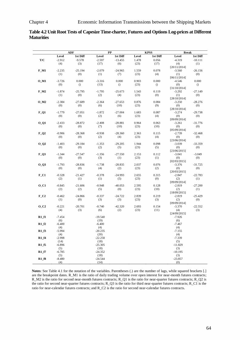
Chapter 4 Economic Information Transmissions between the Shipping Markets
64
Table 4.2 Unit Root Tests of Capesize Time-charter, Futures and Options Log-prices at Different
Maturities
ADF PP KPSS Break
Level 1st Diff Level 1st Diff Level 1st Diff Level 1st Diff
T/C -2.912 -9.578 -2.597 -13.455 1.478 0.056 -4.319 -10.111 (4) (3) (17) (6) (23) (17) (4) (1)
[20/11/2014] F_M1 -2.235 -25.194 -2.079 -24.965 1.559 0.078 -3.560 -26.156
(1) (0) (1) (7) (23) (4) (1) (0) [06/11/2014]
O_M1 -3.726 0.000 -3.316 0.000 0.903 0.000 -4.546 0.000 (0) () (13) () (23) () (0) ()
[31/10/2014] F_M2 -1.874 -25.795 -1.795 -25.673 1.543 0.119 -3.292 -27.149
(1) (0) (2) (4) (23) (0) (1) (0) [28/10/2014]
O_M2 -2.384 -27.689 -2.364 -27.653 0.876 0.084 -3.250 -28.276 (0) (0) (6) (10) (23) (9) (0) (0)
[28/10/2014] F_Q1 -1.779 -27.051 -1.872 -27.004 1.683 0.087 -3.274 -29.738
(0) (0) (2) (6) (23) (4) (0) (0) [09/09/2014]
O_Q1 -2.433 -28.872 -2.408 -28.881 0.964 0.063 -3.261 -31.776 (0) (0) (7) (10) (23) (10) (0) (0)
[05/09/2014] F_Q2 -0.906 -28.368 -0.938 -28.360 2.363 0.115 -2.739 -32.468
(0) (0) (2) (4) (23) (4) (0) (0) [23/06/2014]
O_Q2 -1.403 -29.184 -1.353 -29.205 1.944 0.098 -3.039 -33.359 (0) (0) (2) (5) (23) (5) (0) (0)
[23/06/2015] F_Q3 -1.344 -27.547 -1.356 -27.550 2.153 0.112 -3.041 -3.049
(0) (0) (3) (1) (23) (1) (0) (0)
[02/03/2015] O_Q3 -1.793 -28.836 -1.738 -28.835 2.037 0.076 -3.376 -31.725
(0) (0) (4) (2) (23) (2) (0) (0) [20/03/2015]
F_C1 -0.328 -21.427 -0.378 -24.993 2.655 0.315 -2.847 -22.783 (2) (1) (1) (5) (23) (0) (2) (1)
[09/09/2014] O_C1 -0.845 -21.606 -0.948 -40.053 2.595 0.128 -2.819 -27.200
(2) (2) (5) (0) (23) (10) (2) (1) [18/09/2015]
F_C2 -0.462 -24.866 -0.337 -24.722 2.839 0.219 -2.819 -25.429 (1) (0) (3) (3) (23) (3) (2) (0)
[09/09/2014] O_C2 -0.221 -20.701 -0.740 -42.320 2.693 0.154 -3.370 -22.552
(4) (3) (6) (2) (23) (11) (4) (3) [24/09/2015]
R1_f1 -7.454 -19.540 -7.926 (6) (19) (6)
R1_f2 -6.400 -6.400 -7.467 (4) (4) (4)
R1_f3 -5.994 -20.235 -7.155 (4) (20) (4)
R1_f4 -2.998 -22.258 -7.339 (14) (18) (5)
R1_f5 -6.896 -25.305 -11.829 (5) (18) (3)
R1_f7 -6.785 -24.352 -10.195 (5) (18) (3)
R1_f8 -8.480 -24.544 -23.857 (4) (14) (0)
Notes: See Table 4.1 for the notation of the variables. Parentheses (.) are the number of lags, while squared brackets [.]
are the breakpoint dates. R_M1 is the ratio of daily trading volume over open interest for near-month futures contracts;
R_M2 is the ratio for second near-month futures contracts; R_Q1 is the ratio for near-quarter futures contracts; R_Q2 is
the ratio for second near-quarter futures contracts; R_Q3 is the ratio for third near-quarter futures contracts; R_C1 is the
ratio for near-calendar futures contracts; and R_C2 is the ratio for second near-calendar futures contracts.

Chapter 4 Economic Information Transmissions between the Shipping Markets
65
Table 4.3 Cointegration Tests for Capesize Vessels
Lags Johansen Johansen with structural break
max trance max trance
Ho H1 Ho H1 Ho H1 Ho H1
r = 0 r = 1 r = 0 r = 1 r = 0 r = 1 r = 0 r = 1
r <= 1 r = 2 r <= 1 r = 2 r <= 1 r = 2 r <= 1 r = 2
r <=2 r = 3 r <=2 r = 3 r <=2 r = 3 r <=2 r = 3
Break-point
T/C — F_M1 - O_M1 – – – –
T/C —F_M2 — O_M2 2 21.782 21.131 39.818 29.797
14.515 14.264 18.036 15.494
3.521 3.841 3.521 3.841
T/C — F_Q1 — O_Q1 2 16.816 21.131 33.771 29.797
13.29 14.264 16.954 15.494
3.663 3.841 3.663 3.8414
T/C — F_Q2 — O_Q2 2 11.182 21.131 20.099 29.797
8.250 14.264 8.917 15.497
0.667 3.841 0.667 3.841
T/C — F_Q3 — O_Q3 2 15.214 21.131 26.535 29.797
11.099 14.264 11.320 15.494
0.221 3.841 0.221 3.841
T/C — F_C1 — O_C1 2 27.652 21.131 36.484 29.797
8.801 14.264 8.832 15.494
0.031 3.841 0.031 3.8414
T/C — F_C2 — O_C2 2 15.394 21.131 27.358 29.79& 56.688 43.460 69.178 59.090
11.868 14.264 11.964 15.494 11.414 26.440 12.490 37.420
0.096 3.841 0.096 3.841 1.076 12.850 1.076 18.900
Notes: Lags is the lag length of the Vector Autoregressive (VAR) models used for the cointegration test without a structural
break (Johansen, 1988), and for the cointegration test with a structural break on the constant and slope (Johansen et al.,
2000). The lag length is determined by minimising the SBIC (1978). r represents the number of cointegrating vectors. λi, is
the λmax and λtrace cointegration tests of the estimated eigenvalues of the Π matrix in Equation (1). Critical values for the
λmax and λtrace statistics for cointegration without a structural break and cointegration with a structural break are calculated
and provided under alternate hypothesis.
Overall, distant-maturity contracts, for all three types of vessels exhibit cointegrating
relationships with their corresponding time-charter rates. The coefficient of the error-
correction terms is significant and negative, indicating that the documented cointegrating
relationship among the investigated markets acts as a buffer to any external shocks keeping

Chapter 4 Economic Information Transmissions between the Shipping Markets
66
them together in a long-run equilibrium relationship.30 This may be the result of the supply of
newbuilding vessels matching cargo requirements, as shipyards typically take some time to
deliver a vessel.31 As the size of the orderbook helps in anticipating freight rates, the time
period between the order and delivery of newbuilding vessels is matched by the distant-
maturity derivatives contracts. Furthermore, near-maturity derivatives contracts also appear
to exhibit long-run relationships with time-charter rates for all three types of vessels, with the
error-correction terms being significant and negative, similar to the case of distant-maturity
contracts. 32 This may be due to the liquidity of the freight futures contracts, as it is
significantly higher for near-maturity contracts (explained in the later part of the study),
resulting in a strong adjustment of near-maturity derivatives prices to the time-charter prices.
4.3.2. Spillover effect on returns and volatilities
Tables 4.4 and 4.5 present the spillover effects results of returns and volatilities between
time-charter rates and corresponding freight futures and options prices, for the three-major
dry-bulk vessels under different contract maturities. VECM models are used when
cointegration is detected and VAR models when it is not. Panel A presents the interaction
between the returns of the underlying time-charter market and the two derivatives markets,
along with the trading activity of futures markets. In the system of equations, some variables
are found to be weakly statistically significant jointly, although individually fail to explain
the dependent variable. Wald tests are conducted to understand whether individual markets
(say, the freight options market) are sufficient to explain the dependent market (say, the
physical time-charter market) or just have an explanatory power only in the presence of
stronger markets (say, the freight futures markets). Panel B shows the interactions of
volatilities between the time-charter rates, freight futures and options prices. The empirical
findings are as follows.
4.3.2.1. Spillover effects under cointegrating relationships
Table 4.4 presents sixteen models where cointegrating relationships are found between time-
charter rates, freight futures and freight options prices for different vessels. These are: (i)
30 Near-calendar and second near-calendar contracts for Capesize (C_C1 and C_C2), Panamax (P_C1 and P_C2) and
Supramax (S_C1 and S_C2) vessels. 31 Delivery time and availability of slots vary from one shipyard to another. If there is relatively no waiting time delivery
typically takes from 12 to 24 months. 32 Second near-month and near-quarter contracts for Panamax (P_M2 and P_Q1), from near-month to near-quarter contracts
for Supramax (S_M1, S_M2 and S_Q1) and second near-month contracts for Capesize (C_M2), except near-quarter
contracts for Capesize (C_Q1).

Chapter 4 Economic Information Transmissions between the Shipping Markets
67
nearby maturity contracts (near-month Supramax (S_M1), second near-month Capesize
(C_M2), Panamax (P_M2) and Supramax (S_M2)); (ii) medium maturity contracts (near-
quarter and second near-quarter Panamax (P_Q1 and P_Q2) and Supramax (S_Q1 and S_Q2)
and third near-quarter Supramax (S_Q3); and (iii) distant maturity contracts (near-calendar
and second near-calendar Capesize (C_C1 and C_C2) and Panamax (P_C1 and P_C2) and
Supramax (S_C1 and S_C2)). In Panel A, the lagged error-correction terms ect1 and ect2
(ect2 is presented only in the case where two cointegrating vectors are established) are
significant in all cases with at least one cointegrating vector in the regression model being
significant. Most of the ect coefficients (speed of adjustment) are negative, indicating that
variables that divert from the cointegrating relationship increase in value to restore the long-
run equilibrium relationship.
Firstly, according to the short-run dynamics of the models, lagged time-charter rates
significantly explain most of the futures prices (apart from the second near-quarter (S_Q2)
Supramax regression), while all lagged futures prices significantly explain time-charter rates,
apart from one regression (near-quarter (S_Q1) Supramax). This indicates that there is a bi-
directional spillover effect in returns between the time-charter market and the futures market,
but according to a Wald (joint significance) test, this effect runs stronger from the futures
(derivatives) market towards the time-charter (underlying) freight market.
Secondly, in terms of the interaction between freight futures and freight options returns,
lagged options prices significantly explain futures prices only in eight out of sixteen models
(second near-month (P_M2) and second near-quarter (P_Q2) Panamax, and near-month
(S_M1), second near-month (S_M2), second near-quarter (S_Q2), third near-quarter (S_Q3),
near-calendar (S_C1) and second near-calendar (S_C2) Supramax), while lagged futures
prices significantly explain freight options prices in all sixteen models. Also, the joint impact
(according to a Wald test) of freight futures returns on freight options returns is stronger than
the reverse, indicating that the freight futures market is informationally leading the freight
options market.
Thirdly, results on the interaction between lagged time-charter rates and lagged freight
options prices indicate that time-charter returns significantly explain freight options returns
for all models apart from four regressions (second near-month (P_M2) Panamax, and near-
month (S_M1) near-quarter (S_Q1) and second near-calendar (S_C2) Supramax). In contrast,
lagged freight options returns can explain time-charter rates only in seven (out of sixteen)
Chapter 4 Economic Information Transmissions between the Shipping Markets
68
models (near-calendar (C_C1) Capesize, near-quarter (P_Q1), second near-quarter (P_Q2),
third near-quarter (P_Q3), near-calendar (P_C1) and second near-calendar (P_C2) Panamax
and near-quarter (S_Q1) Supramax). This rather unexpected result indicates that the time-
charter (underlying) market is informationally leading the freight options (derivatives)
market, which is inconsistent with conventional wisdom and expectations. Overall, results
from Wald joint tests suggest that information in returns is transmitted first from the freight
futures market to the time-charter market, and then is spilt over to the freight options market.
Panel B of Table 4.4 presents the parameter estimates of the conditional variance models.
The 𝑏𝑗𝑗 coefficient is significant in all regressions indicating a strong volatility spillover
between time-charter rates and the corresponding freight futures and freight options prices for
all three vessel types. Also, the 𝑐𝑗𝑗 coefficient is significant in all models (except for near-
month (S_M1) Supramax), indicating that a shock (either positive or negative) can be
transmitted, say, from the futures market to the time-charter or options market, leading to an
increase in the latter market’s volatility. Furthermore, the leverage effect 𝑑𝑗𝑗 coefficient for
time-charter rates is statistically significant in eleven (out of sixteen) models (apart from
near-calendar (C_C1) Capesize, second near-quarter (P_Q2) Panamax, second near-month
(S_M2), near-quarter (S_Q1) and second near-calendar (S_C2) Supramax), indicating that a
negative shock generated in the time-charter market does not necessarily result in increasing
volatilities in other markets, as compared to a positive shock of the same magnitude. In
contrast, the leverage volatility effect is more prevalent in the derivatives markets, as it is
observed in all sixteen models. This could be a result of the increased flexibility of
derivatives contracts over physical trades, as discussed earlier. Accordingly, open positions in
freight derivatives markets can be closed almost immediately upon the arrival of bad news,
resulting in an increase in market volatility.
4.3.2.2. Spillover effects under non-cointegrating relationships
Table 4.5 presents five models where cointegrating relationships (with or without structural
breaks) are not found between time-charter rates, freight futures and options prices for
different vessel types. These are: (i) nearby maturity contracts (near-month Capesize (C_M1)
and Panamax (P_M1)); and (ii) medium maturity contracts (near-quarter (C_Q1), second
near-quarter C_Q2) and third near-quarter (C_Q3) Capesize).

Chapter 4 Economic Information Transmissions between the Shipping Markets
69
In Panel A, the coefficients of the lagged returns indicate the presence of significant short-run
relationships between time-charter rates, freight futures and options prices. Firstly, lagged
freight futures prices significantly explain time-charter rates in four (out of five) models
(C_M1, C_Q1, C_Q3 and P_M1), and also in four models (C_Q1, C_Q2, C_Q3 and P_M1)
the lagged time-charter rates can significantly explain futures prices. These results indicate a
bi-directional spillover effect between the freight futures and the time-charter markets, but
with stronger information flow from the futures (derivatives) market to the time-charter
(underlying) market using a Wald test, which is in accordance with both theory and
expectations.
Secondly, results on the interactions between freight futures and freight options prices
indicate that freight futures returns significantly explain options returns in four (out of five)
models (C_M1, C_Q1, C_Q3, and P_M1), while freight options returns can explain futures
returns in four models (C_M1, C_Q1, C_Q3, and P_M1). Also, based on the magnitude of
the joint significance of the lagged variables (Wald test), the results point to stronger
spillover effects from the freight futures market to the freight options market. Thirdly, it can
be seen that time-charter rates can significantly explain freight returns can explain time-
charter rates in only three cases (C_M1, C_Q3 and P_M1). These results confirm the
presence of a bi-directional flow of information between time-charter returns and freight
options returns. Wald joint tests indicate that new market information is first reflected in the
futures market before it is spilt into the time-charter market, and finally appears in the options
market.
Panel B of Table 4.5 presents the parameter estimates of the conditional variance models. It is
observed that the 𝑏𝑗𝑗 coefficient is significant in all models, indicating an existence of
volatility spillovers between time-charter, freight futures and options markets. The 𝑐𝑗𝑗
coefficient is statistically significant in all models (except in C_Q2 and C_Q3), indicating
that a shock (either positive or negative) can be transmitted between the three markets,
similarly to the results in the previous section for cointegrating models. Finally, the leverage
volatility effect, according to the 𝑑𝑗𝑗 coefficient, is observed in four models for the
derivatives markets (C_M1, C_Q1, C_Q2 and P_M1), but only in three models for the time-
charter market (C_M1, C_Q1 and P_M1).

Chapter 4 Economic Information Transmissions between the Shipping Markets
70
Table 4.4 Maximum-likelihood Estimates of Restricted BEKK VECM-GARCH Models
Notes: a Significance at the 1% significance level. b Significance at the 5% significance level.
c Significance at the 10% significance level.
C_M2 C_C1 C_C2 P_M2 P_Q1 P_Q2 P_Q3 P_C1
(T/C) (T/C) (T/C) (T/C) (T/C) (T/C) (T/C) (T/C)
(Futures) (Futures) (Futures) (Futures) (Futures) (Futures) (Futures) (Futures)
(Options) (Options) (Options) (Options) (Options) (Options) (Options) (Options)
Panel A: Conditional mean parameters
ect1 -0.022a -0.005b -0.004a -0.0003 -0.001b -0.004a -0.003a -0.003a
-0.017a 0.004 a 0.000 0.000 -0.002 -0.006a 0.008a 0.001
-0.019a 0.010a 0.001a -0.020a -0.012a -0.019a 0.002 0.000
ect2 0.031a — — — — — — -0.002
0.036a — — — — — — -0.038a
0.078a — — — — — — 0.032a
T/C (lag 1) 0.555a 0.551a 0.602a 0.871a 0.872a 1.012a 1.104a 1.008a
-0.095a -0.121a -0.044a 0.081a 0.070c 0.269a 0.173a 0.103b
-0.098a -0.180a -0.035a 0.039 -0.101a 0.278a 0.192a 0.136c
Futures (lag 1) 0.311a 0.808a 1.164a 0.074a 0.037a -0.004 -0.008 0.129a
0.205b 0.278a 0.393a 0.386a 0.215a -0.227a 0.207a 0.303a
0.290a 0.451a 0.650a 0.522a 0.091b -0.281a 0.302a 0.379a
Options (lag 1) -0.036 0.104a 0.040 -0.0001 0.018a 0.036a 0.052a 0.018b
-0.072 -0.021 0.004 -0.094a -0.031 0.055a 0.014 -0.019
-0.135c -0.078 -0.120a -0.172a 0.057c 0.011 0.093a -0.049
T/C (lag 2) — — — — — -0.167a -0.239a -0.175a
— — — — — -0.519a -0.234a -0.193a
— — — — — -0.574a -0.193a -0.229a
Futures (lag 2) — — — — — 0.020 0.012 0.012
— — — — — -0.192a 0.069b -0.132a
— — — — — -0.135a 0.096a -0.382a
Options (lag 2) — — — — — 0.006 0.013 0.005
— — — — — 0.002 -0.025 -0.008
— — — — — -0.091c -0.015 0.241a
Ratio (lag 1) 0.004a 0.001 0.0007 0.0002 0.0002 0.000 -0.0001 0.0004
0.003a -0.0001 0.0005c -0.0006 0.001c 0.000 -0.001a 0.0001
0.006a 0.0004 0.0009a 0.000 0.001a 0.003a -0.0003 0.0002
Wald Test
Futures → T/C 34.95a 95.61a 85.02a 49.39a 31.66a 0.90 0.64 29.80a
Options → T/C 0.76 3.97b 2.11 0.04 15.94a 9.29b 16.72a 10.82a
Joint → T/C 101.53a 120.37a 98.41a 101.06a 100.14a 30.49a 51.23a 59.94a
T/C → Futures 9.33a 24.67a 12.71a 0.64 0.23 14.11a 10.37a 10.59a
Options → Futures 1.59 0.25 0.2 0.94 0.37 0.65 0.33 2.68
Joint → Futures 10.57a 24.84a 12.93a 1.43 0.61 15.04a 10.5b 13.14b
T/C → Options 8.64a 11.79a 3.76b 3.15c 0.37 7.31a 3.69 0.02
Futures → Options 10.84a 112.07a 28.27a 9.86a 18.74a 20.03a 43.54a 101.73a
Joint → Options 16.65a 113.78a 28.99a 11a 18.74a 31.83a 54.76a 116.48a
Panel B: Conditional variance parameters
ajj 6.33e-05a 0.000277a 0.000208a 1.8e-05a 3.2e-05a 4.44e-05a 2.24e-05a 4.81e-05a
2.33e-05a 3.02E-07 8.17e-06a 2.2e-05a 0.000208a 9.95e-06a 0.000196a 3.77e-06a
-2.88e-05a -7.34e-06a 3.54E-07 -2.23E-05 0.000466a 1.91e-05a 0.000282a 7.97e-06a
cjj 0.202a 0.455a 0.324a 0.631a 0.549a 0.666a 0.479a 0.681a
0.077a 0.270a 0.322a 0.106a 0.666a 0.575a 1.296a 0.479a
0.050b 0.293a 0.378a 0.056c 1.497a 0.539a 1.372a 0.573a
djj 0.156a -0.063 0.231a 0.151c -0.261a 0.119 0.191b -0.455a
0.198a -0.111a 0.616a 0.380a 0.850a -0.414a -1.221a 0.304a
0.194a 0.342a 0.693a 0.897a 2.051a -0.781a -1.590a 0.610a
bjj 0.960a 0.837a 0.897a 0.695a 0.648a 0.436a 0.760a -0.271a
0.985a 0.964a 0.899a 0.954a 0.651a 0.857a 0.148a 0.899a
0.994a 0.957a 0.904a 0.904a 0.224a 0.839a 0.0821b 0.861a

Chapter 4 Economic Information Transmissions between the Shipping Markets
71
Table 4.4 Maximum-likelihood Estimates of Restricted BEKK VECM-GARCH Models (cont.)
P_C2 S_M1 S_M2 S_Q1 S_Q2 S_Q3 S_C1 S_C2
(T/C) (T/C) (T/C) (T/C) (T/C) (T/C) (T/C) (T/C)
(Futures) (Futures) (Futures) (Futures) (Futures) (Futures) (Futures) (Futures)
(Options) (Options) (Options) (Options) (Options) (Options) (Options) (Options)
Panel A: Conditional mean parameters
ect1 -0.001c -0.010a -0.016a -0.010a 0.0004b 0.001 0.001a -0.004a
0.001 -0.0004 -0.012b 0.002 0.002a 0.009a 0.001b -0.0008
0.003b -0.016b -0.012a 0.001 0.008a 0.018a 0.003a 0.000
ect2 — 0.008c 0.014a -0.003 — — — —
— -0.005 -0.003 -0.010 — — — —
— 0.164a 0.191a 0.167a — — — —
T/C (lag 1) 1.070a 0.834a 0.676a 0.860a 0.888a 0.880a 0.857a 0.878a
0.122a 0.858a 0.321a 0.311a 0.028 0.370a 0.104c 0.134b
0.302a 0.218 0.286a 0.003 0.114c 0.332a -0.475a 0.046
Futures (lag 1) 0.195a 0.023c -0.023b -0.008 0.018b 0.023 0.098a -0.064a
0.304a 0.276a 0.421a 0.404a 0.078c 0.086b 0.401a 0.248a
0.759a 0.451a 0.439a 0.439a 0.006 0.360a 0.579a 0.548a
Options (lag 1) 0.015a -0.002 -0.003 -0.008a -0.014c -0.018c -0.007 -0.005
0.008 -0.017c -0.061a -0.018 0.030b -0.022 0.002 -0.009
-0.137a -0.025 -0.069c -0.043 0.072b -0.207a -0.073 -0.092b
T/C (lag 2) -0.223a 0.0580 0.250a 0.152a -0.002 0.0231 -0.004 0.139a
-0.136a -0.561a -0.327a -0.330a 0.032 -0.081 -0.158a -0.119b
-0.287a -0.051 -0.363a -0.389b -0.327a -0.162 0.0134 0.0176
Futures (lag 2) -0.026 -0.007 -0.027a -0.006 -0.021a -0.015 -0.008 -0.102a
-0.115a -0.065 -0.006 0.009 -0.251a -0.049 -0.081b -0.049
-0.377a -0.118b -0.090 -0.024 -0.081b -0.060 -0.016 -0.306a
Options (lag 2) 0.004 -0.001 -0.001 -0.006 -0.014c -0.006 -0.003 -0.007c
-0.0004 -0.009 -0.029 -0.028 -0.030c -0.0478a -0.011a -0.019a
0.104a -0.001 -0.044 -0.048 -0.220a -0.118c 0.0125 0.0073
Ratio (lag 1) 0.0001 0.0001 0.0003a -0.0003b -0.0001 -0.0001 -0.0002b 0.0001
0.0002 -0.0004 -0.001 -0.0003 -0.002a 0.002a -0.0001 0.000
0.0005 -0.002a 0.001 0.000 -0.0002 0.002a -0.0001 0.001a
Wald Test
Futures → T/C 39.10a 1.04 9.15a 6.46b 1.03 4.68c 3.25 2.49
Options → T/C 5.01c 0.46 0.18 0.71 0.95 1.76 0.37 2.61
Joint → T/C 52.81a 1.30 10.55b 8.78c 2.25 6.86 3.88 5.84
T/C → Futures 12.85a 18.44a 10.87a 15.35a 2.52 5.78c 3.28 0.42
Options → Futures 3.45a 2.55 1.36 3.12 1.28 0.47 2.62 5.6c
Joint → Futures 15.69a 21.43a 12.48b 17.23a 3.82 6.25 5.71 6.25
T/C → Options 7.22a 0.96 1.03 4.94c 0.08 0.63 3.79 1.12
Futures → Options 16.83a 0.92 4.72c 12.62a 12.22a 46.68a 49.35a 26.55a
Joint → Options 32.36a 2.49 6.14 18.79a 12.52b 47.65a 49.58a 26.94a
Panel B: Conditional variance parameters
ajj 4.1e-05a 3.52e-05b 1.8e-05a 4.9e-06a 1.3e-06a 1.63e-06a 1.61e-06a 6.53e-06a
2.79e-06a 2.78e-05a 0.000167a 0.000335a 8.43e-06a 9.05e-06a 4.69e-06a 9.3e-07a
2.14E-06 0.000294a 6.95e-05a 9.13e-05a -2.48E-06 -2.51E-06 1.05E-06 -1.15E-06
cjj 0.672a 0.1727 1.038a 0.769a 0.167a -0.426a 0.251a 0.751a
-0.137a 0.0222 0.180a 0.172b 0.860a 0.048 0.390a 0.235a
-0.381a 0.0114 0.056 0.090a 1.121a 0.212a 0.692a 0.514a
djj 0.354a -0.202b 0.065 0.0588 -0.708a -0.583a 0.678a 0.024
0.257a -0.257a 0.791a -0.371b 0.127 -0.727a -0.094c -0.248a
0.607a -2.25a 1.181a -1.25a 0.438a -0.749a -0.543a -0.454a
bjj 0.410a 0.418 0.094 0.733a 0.907a 0.882a 0.892a 0.721a
0.966a 0.963a 0.728a 0.554a 0.839a 0.897a 0.918a 0.965a
0.906a 0.604a 0.804a 0.760a 0.762a 0.902a 0.847a 0.911a

Chapter 4 Economic Information Transmissions between the Shipping Markets
72
Table 4.5 Maximum-likelihood estimates of Restricted BEKK VAR-GARCH Models
Notes: The significance levels of the coefficient parameters are denoted in Table 4.4.
C_M1 C_Q1 C_Q2 C_Q3 P_M1
(T/C) (T/C) (T/C) (T/C) (T/C)
(Futures) (Futures) (Futures) (Futures) (Futures)
(Options) (Options) (Options) (Options) (Options)
Panel A: Conditional mean parameters
T/C (lag 1) 0.539a 0.574a 0.660a 0.634a 0.867a
-0.007 -0.132a -0.133a -0.049a 0.133a
-0.064a -0.178a -0.125a -0.064a 0.134a
Futures (lag 1) 0.362a 0.207a 0.051 0.242a 0.052a
0.421a 0.340a -0.087 0.057a 0.211a
0.618a 0.443a 0.068 0.068a 0.675a
Options (lag 1) -0.053a -0.008 0.082 0.145a -0.004b
-0.141a -0.239a 0.111 0.038a -0.080a
-0.249a -0.316a -0.033 0.051a -0.351a
Ratio (lag 1) 0.001 0.0026a 0.0009 0.0014 -0.0001
-0.002a 0.0055a 0.0103a 0.0036a -0.003a
0.001c 0.0063a 0.0104a 0.0057a -0.003a
Wald Test
Futures → T/C 88.04a 18.83a 2.11 37.59a 65.71a
Options → T/C 2.47 1.93 1.18 44.04a 1.75
Joint → T/C 144a 70.15a 33.00a 70.3a 86.2a
T/C → Futures 8.92a 3.02c 8.79a 6.58a 0.01
Options → Futures 4.67a 0.03 0.13 0.54 4.78b
Joint → Futures 12.93a 3.04 9.07b 6.85b 4.92c
T/C → Options 4.48b 4.35b 13.34a 10.72a 3.57c
Futures → Options 15.89a 20.41a 12.74a 5.36b 9.16a
Joint → Options 16.87a 22.31a 23.62a 16.12a 10.42a
Panel B: Conditional variance parameters
ajj 7.68e-05a 0.0003a 0.001a 0.0004a 1.33e-05a
1.61E-05 2.27e-05a -1.67e-06a 1.98e-07c 8.09e-05a
-0.0001a 4.14e-05c 2.33e-06a 2.00E-07 8.23e-05a
cjj 0.160a 0.303a 0.836a 0.579a 0.573a
0.333a 0.718a -0.007 2.40E-05 0.283a
0.157a 1.171a -0.006 0.001 0.212a
djj 0.255a 0.193a 0.006 2.07E-06 0.198b
0.712a 1.181a 0.037a 1.14E-08 0.897a
1.427a 0.733a 0.066a 4.60E-08 3.569a
bjj 0.956a 0.887a 0.360a 0.750a 0.763a
0.895a 0.757a 1.001a 1.001a 0.873a
0.850a 0.692a 1.000a 1.001a 0.744a

Chapter 4 Economic Information Transmissions between the Shipping Markets
73
4.3.3. Impulse response analysis
Generalized Impulse Responses (GIR) functions of a SUR-VAR (when a cointegrating
relationship is not established) and of a SUR-VECM (when a cointegrating relationship is
established) are next estimated to provide insights into the dynamics of the causality effects
between the three investigated markets. Impulse responses measure the reaction of one
market (e.g. time-charter) by inducing one standard deviation shock to the prices of the other
market (e.g. freight futures or options).
Figure 3.1 depicts the impact of a shock on the Capesize market. The upper graphs illustrate
the response of time-charter rates (CTC),33 those in the middle the response of freight futures
prices (CTF), while the lower graphs show the response of freight option prices (CTO)
triggered due to a one standard deviation shock in each respective market. We observe the
market response for a 10 day-ahead horizon. The results indicate that Capesize time-charter
rates are strongly affected by the shock generated in freight futures and freight options prices
irrespective of maturity, with the shock in freight futures having a greater impact. Results
corroborate the same pattern for Panamax rates. Moreover, Capesize and Panamax futures
(options) prices are affected by a corresponding shock generated in time-charter rates and
options (futures) prices, irrespective of maturity. However, it appears that the impact of the
shock diminishes faster in the freight futures market than in the time-charter market,
indicating that the freight futures market can adapt to shocks more rapidly than the
underlying freight market. Supramax time-charter rates marginally react to a shock generated
in futures prices and do not affect options’ prices at all. This may be due to the low liquidity
of Supramax freight futures contracts and the negligible liquidity of Supramax freight
options. Overall, for all three types of vessels examined, the futures market has stronger
effects in the other two markets (time-charter and freight options) than the time-charter
market, while the freight options market has the least significant impact. These results
indicate that market participants should still rely on freight futures prices to gain a view of
the underlying freight market but cannot use freight options markets for price discovery
purposes. Therefore, practitioners who collect and analyse new market information on a daily
33 For example, the upper graphs represent the impact of Capesize time-charter rates (CTC) to a one standard-deviation
shock on near-month futures (CTF_1M), near-month options (CTO_1M), second near-month futures (CTF_2M), second
near-month options (CTO_2M), near-quarter futures (CTF_1Q), near-quarter options (CTO_1Q), second near-quarter
futures (CTF_2Q), second near-quarter options (CTO_2Q), third near-quarter futures (CTF_3Q), third near-month options
(CTO_3Q), near-calendar futures (CTF_1C), near-calendar options (CTO_1C), second near-calendar futures (CTF_2C) and
second near-calendar options (CTO_2C).

Chapter 4 Economic Information Transmissions between the Shipping Markets
74
basis should investigate freight futures markets first, as any new information is revealed there
before it is spilt over to the physical time-charter market, and finally to the freight options
market.

Chapter 4 Economic Information Transmissions between the Shipping Markets
75
Figure 4.1 Impulse Responses for Capesize Markets
.00
.01
.02
.03
.04
.05
.06
1 2 3 4 5 6 7 8 9 10
D(CTC) D(CTF_M1) D(CTO_M1)
Response of D(CTC) to Generalized One
S.D. Innovations
-.02
.00
.02
.04
.06
.08
.10
1 2 3 4 5 6 7 8 9 10
D(CTC) D(CTF_M1) D(CTO_M1)
Response of D(CTF_M1) to Generalized One
S.D. Innovations
-.04
.00
.04
.08
.12
.16
1 2 3 4 5 6 7 8 9 10
D(CTC) D(CTF_M1) D(CTO_M1)
Response of D(CTO_M1) to Generalized One
S.D. Innovations
.00
.01
.02
.03
.04
.05
.06
1 2 3 4 5 6 7 8 9 10
D(CTC) D(CTF_M2) D(CTO_M2)
Response of D(CTC) to Generalized One
S.D. Innovations
-.02
.00
.02
.04
.06
.08
1 2 3 4 5 6 7 8 9 10
D(CTC) D(CTF_M2) D(CTO_M2)
Response of D(CTF_M2) to Generalized One
S.D. Innovations
-.02
.00
.02
.04
.06
.08
.10
1 2 3 4 5 6 7 8 9 10
D(CTC) D(CTF_M2) D(CTO_M2)
Response of D(CTO_M2) to Generalized One
S.D. Innovations
.00
.01
.02
.03
.04
.05
.06
1 2 3 4 5 6 7 8 9 10
D(CTC) D(CTF_Q1) D(CTO_Q1)
Response of D(CTC) to Generalized One
S.D. Innovations
-.02
.00
.02
.04
.06
.08
1 2 3 4 5 6 7 8 9 10
D(CTC) D(CTF_Q1) D(CTO_Q1)
Response of D(CTF_Q1) to Generalized One
S.D. Innovations
-.02
.00
.02
.04
.06
.08
.10
1 2 3 4 5 6 7 8 9 10
D(CTC) D(CTF_Q1) D(CTO_Q1)
Response of D(CTO_Q1) to Generalized One
S.D. Innovations
.00
.01
.02
.03
.04
.05
.06
1 2 3 4 5 6 7 8 9 10
D(CTC) D(CTF_Q2) D(CTO_Q2)
Response of D(CTC) to Generalized One
S.D. Innovations
-.02
.00
.02
.04
.06
1 2 3 4 5 6 7 8 9 10
D(CTC) D(CTF_Q2) D(CTO_Q2)
Response of D(CTF_Q2) to Generalized One
S.D. Innovations
-.02
.00
.02
.04
.06
1 2 3 4 5 6 7 8 9 10
D(CTC) D(CTF_Q2) D(CTO_Q2)
Response of D(CTO_Q2) to Generalized One
S.D. Innovations

Chapter 4 Economic Information Transmissions between the Shipping Markets
76
Figure 4.1 Impulse Responses for Capesize Markets (cont.)
.00
.01
.02
.03
.04
.05
.06
1 2 3 4 5 6 7 8 9 10
D(CTC) D(CTF_Q3) D(CTO_Q3)
Response of D(CTC) to Generalized One
S.D. Innovations
-.02
.00
.02
.04
.06
1 2 3 4 5 6 7 8 9 10
D(CTC) D(CTF_Q3) D(CTO_Q3)
Response of D(CTF_Q3) to Generalized One
S.D. Innovations
-.02
.00
.02
.04
.06
.08
1 2 3 4 5 6 7 8 9 10
D(CTC) D(CTF_Q3) D(CTO_Q3)
Response of D(CTO_Q3) to Generalized One
S.D. Innovations
.00
.01
.02
.03
.04
.05
.06
1 2 3 4 5 6 7 8 9 10
D(CTC) D(CTF_C1) D(CTO_C1)
Response of D(CTC) to Generalized One
S.D. Innovations
-.005
.000
.005
.010
.015
.020
.025
1 2 3 4 5 6 7 8 9 10
D(CTC) D(CTF_C1) D(CTO_C1)
Response of D(CTF_C1) to Generalized One
S.D. Innovations
-.02
.00
.02
.04
.06
1 2 3 4 5 6 7 8 9 10
D(CTC) D(CTF_C1) D(CTO_C1)
Response of D(CTO_C1) to Generalized One
S.D. Innovations
.00
.01
.02
.03
.04
.05
.06
1 2 3 4 5 6 7 8 9 10
D(CTC) D(CTF_C2) D(CTO_C2)
Response of D(CTC) to Generalized One
S.D. Innovations
-.004
.000
.004
.008
.012
.016
1 2 3 4 5 6 7 8 9 10
D(CTC) D(CTF_C2) D(CTO_C2)
Response of D(CTF_C2) to Generalized One
S.D. Innovations
-.02
.00
.02
.04
.06
1 2 3 4 5 6 7 8 9 10
D(CTC) D(CTF_C2) D(CTO_C2)
Response of D(CTO_C2) to Generalized One
S.D. Innovations

Chapter 4 Tracing Lead-Lag Relationships between Commodities and Freights
77
4.3.4. Price-trading activities and liquidity measure
In the literature, there is a strong linkage between the trading activities of stock prices with
other asset class prices (Bessembinder, 1992, Bessembinder et al., 1996, Bessembinder and
Seguin, 1993, Lee and Swaminathan, 2000, Tauchen and Pitts, 1983). Along these lines, in
Table 4.4, we observe a strong interaction between freight futures trading activity (𝑅𝑎𝑡𝑖𝑜𝑡−1)
and freight derivatives (futures and options) prices. Specifically, for Capesize vessels, the
lagged ratio of futures trading volume over open interest significantly affects futures and
options prices for near to medium distance maturity derivatives contracts (near-month
(C_M1), second near-month (C_M2) and near-quarter (C_Q1), second near-quarter (C_Q2)
and third near-quarter (C_Q3)), but does not affect time-charter rates at all, except second
near-month (C_M2) and near-quarter (C_Q1). For Panamax vessels, the futures trading
activities affect near-maturity futures and options contracts only (near-month (P_M1) and
near-quarter (P_Q1)). In contrast to Capesize time-charter rates, Panamax time-charter rates
are not affected by futures trading activities. Similar to Capesize and Panamax time-charter
rates, Supramax time-charter rates are not affected by trading activities futures contracts
except second near-month (S_M2), near-quarter (S_Q1) and near-calendar (S_C1) contracts.
Supramax freight futures and options prices are only influenced by the trading activities of
third near-quarter (S_Q3) futures together. It seems that freight futures trading activities
cannot sufficiently explain time-charter rates for either vessel type.
In order to also examine if the options trading activities affect time-charter, futures and
options prices, we estimate the ratio of options trading volume over options open interest
(from LCH.Clearnet) for 21 models’ overall different maturities. Only 10 models could be
estimated (as the open-interest dropped to zero for all others) with three endogenous variables
in each case, adding up to 30 price relationships altogether. Untabulated results indicate that
only five (out of 30) price relationships are found to be affected by options trading activities
(options prices in C_Q2 and P_M1 maturities, futures’ prices in C_Q2 and P_Q1 maturities,
and time-charter prices for P_M2 maturity). Consequently, it seems that options trading
activities are not significantly affecting time-charter, futures or options prices in most cases,
which is in line with the rest of our results.
In an attempt to explain the unexpected results relating to the freight options market, Table
4.6 reports the Amivest liquidity measure results of time-charter, freight futures and options

Chapter 4 Tracing Lead-Lag Relationships between Commodities and Freights
78
contracts for Capesize, Panamax and Supramax contracts for different maturity periods.
Evidently, the liquidity of futures contracts is more than that of options contracts for all
vessel types. This may justify the slower reaction of freight options to new market
information relative to freight futures, due to the lack of active market practitioners in the
freight options’ market.
It is also observed that near-month futures contracts (F_M1) are more liquid than second
near-maturity futures contracts (F_M2) for Capesize and Supramax vessels, but second near-
maturity futures contracts (F_M2) are more liquid than near-month futures contracts (F_M1)
for Panamax vessels. Considering quarter-ahead and calendar-ahead contracts, near-quarter
futures contracts (F_Q1) are subject to the highest degree of liquidity for all types of vessels.
Second near-calendar freight futures (F_C2) contracts are negligible in terms of liquidity for
all three types of vessels.
The results indicate that freight futures contracts with higher liquidity produce a strong
information transmission compared to freight futures with lower market liquidity. Capesize
freight options contracts are the most traded, followed by Panamax options, while Supramax
options contracts are the most illiquid. Since Capesize time-charter rates are more volatile
than Panamax time-charter rates, shipowners and charterers are more interested in securing
long-term freight rates for the Capesize market, leading to higher liquidity for distant-
maturity Capesize futures contracts (than Panamax futures contracts), as observed in Table
4.6. Overall, the low liquidity of freight options may be the main factor behind the poor price
discovery results documented in the previous section.34
Table 4.6 Amivest Liquidity Ratio for Futures and Options at Different Maturity Periods
Notes: CAPE, PMAX and SUPRA represent the Capesize, Panamax and Supramax markets, respectively. Futures and
options contract maturities are as defined in Table 4.1. The table reports the liquidity ratio of freight futures and options
markets for various maturities for the three vessel categories using the Amivest liquidity measure, where a higher liquidity
ratio represents higher liquidity in the respective market.
34 In order to verify that there is no possible measurement bias in the Amivest ratio, similar to the one in the Amihud ratio,
we also re-estimated the Amivest ratio based on a weekly sample period and the (untabulated) results are qualitatively the
same; that is, options liquidity is significantly lower than futures liquidity for all three vessel types over the different
maturities.
F_M1 O_M1 F_M2 O_M2 F_Q1 O_Q1 F_Q2 O_Q2 F_Q3 O_Q3 F_C1 O_C1 F_C2 O_C2
CAPE 1387 162 989 113 1433 201 641 211 544 208 914 150 - 12
PMAX 1290 5 1392 26 1735 35 593 25 582 31 528 13 - 12
SUPRA 417 - 373 - 474 - 272 - 231 - 195 - - -

Chapter 4 Tracing Lead-Lag Relationships between Commodities and Freights
79
4.4. Discussion
In this study, a system with endogenous time-charter rates, freight futures prices, and freight
options prices is investigated for the first time. Overall, the results indicate the existence of
bi-directional spillovers, in both returns and volatilities, between: (i) freight futures and time-
charter markets, (ii) freight futures and freight options markets, and (iii) time-charter and
freight options’ markets, with a stronger information flow reported from the former market to
the latter in each case. The stronger information flow from the futures market to the time-
charter market may be attributed to the higher transaction costs associated with the trading of
physical time-charter contracts, contributing to slower assimilation of new information into
prices. As indicated by the Amivest liquidity measure, the stronger information flow from the
futures market to the freight options market is partially driven by the lower liquidity of the
latter, resulting in slower incorporation of new market information. Moreover, the freight
options market receives stronger information spillovers from the physical time-charter
market, possibly due to the higher liquidity costs involved.
The coefficients of the lagged return values for physical time-charter rates, futures and
options demonstrate that the futures (options) market positively affects the time-charter and
options (futures) markets, though the time-charter market negatively affects the futures and
options markets. This suggests that during the sample period, freight derivatives market
movements tend to increase returns of time-charter rates but, conversely, movements of the
physical freight rate market tend to decrease derivatives returns. A possible explanation for
these spillover effects is the shipowners’ perception of the freight rates’ mean-reverting
properties. It has been documented that freight rates revert to their long-run mean levels (see,
for example, Greenwood and Hanson, 2014). Freight rate (and freight futures) prices are
determined by market agents’ expectations, rather than by a strict cost-of-carry (no-arbitrage)
relationship since a freight service is a non-storable commodity. This idiosyncratic feature
makes shipowners expect an increase in freight futures prices when time-charter rates are
low, attesting the mean-reverting property of freight rates.
This can stimulate increased investment in assets (ships) at a lower price to gain high returns
in the near future from a market turnaround. In turn, such strategies can lead to over-supply
of vessels exerting pressure to time-charter rates that remain at low levels, sending negative
signals to the derivatives markets. Accordingly, the positive sentiment for an expected

Chapter 4 Tracing Lead-Lag Relationships between Commodities and Freights
80
improvement in the freight market results in a contango forward curve, where freight
derivatives prices are higher than the underlying freight rates, inflating the orderbook of dry-
bulk vessels, and prolonging the downturn in freight rates.
One important implication of our results is that the freight futures market informationally
leads the physical time-charter market, and can thus be efficiently used as a price discovery
vehicle for dry-bulk freight rates, by attracting participants with both hedging and speculation
trading motives. Interestingly, it seems that the freight options market should not be relied
upon to serve as a price discovery function, as it lags behind both the freight futures and
physical time-charter markets. Instead, the freight options market is probably most relevant
as a vehicle to match willing buyers and sellers for strategic risk hedging, of which at least
one party has an interest in a vessel and charterparty. In order to empirically investigate the
argument that freight futures are mainly used for trading/speculation, whereas freight options
are mainly used for strategic hedging purposes, we follow Alizadeh (2013) and regress the
trading volume of freight derivatives (futures and options) contracts over one-period lagged
freight market volatility. Untabulated results show that for freight futures contracts, in all
three vessel types, there is a weak but statistically significant and negative relationship
between trading volume and volatility. This negative relationship could be resulted due to
information driven trades by a higher number of traders/speculators in the market (Alizadeh,
2013). These results are also consistent with Batchelor et al. (2007), where they argue that an
increase in FFA market volatility lowers market liquidity. In contrast, results show that there
is no significant relationship between freight options contracts and freight market volatility,
indicating that market participants trade freight options contracts irrespective of the volatility
of the freight market for strategic hedging purposes. These new findings for the freight
options’ market, documented here for the first time, can be utilised by shipowners, charterers
and investors when making chartering and budgeting decisions, by freight brokers when
pricing and quoting freight options prices and premiums, and also by regulators when
developing policies for the freight market.
Similar to our main finding that the options market informationally lags behind the spot
market, Stephan and Whaley (1990), Chan et al. (1993), Chiang and Fong (2001) and Chan et
al. (2002), amongst other studies in the general finance literature, highlight that options prices
fall short of fulfilling their price discovery function, which can be partially driven by the
illiquidity of the options markets. More specifically, existing literature suggests that although

Chapter 4 Tracing Lead-Lag Relationships between Commodities and Freights
81
informed practitioners trade in options markets, they have a preference for using “limit
orders”.35 Essentially, in an illiquid market, informed traders place limit orders at prices
which may not reflect the expectations of uninformed traders, making it difficult to attract
willing counterparties to trade such options contracts. This restricts informed traders from
trading freely and thus disseminating information in an illiquid market, which makes options
prices informationally lag behind physical prices. Hence, despite the high degree of inherent
financial leverage offered by the options market, options prices may contain less information
than physical prices due to lower market liquidity.
Another reason for the low market liquidity of freight options contracts may be that
traditional freight option pricing models are less efficient. A strand of literature posits that
freight options prices calculated using the conventional Black (1976) model tend to be
mispriced compared to using other more contemporary pricing models such as Merton’s
jump-diffusion model (Nomikos et al., 2013). Due to this mispricing, the freight options
market fails to attract investors and hedgers, resulting in lower liquidity that may drive a
price discovery function inefficiency. To tackle these problems, there is a need to develop
more efficient freight options pricing models.
Chiang and Fong (2001) argue that another reason could be that market-makers focus on
prices on the more liquid and mature futures market and revise them frequently, whereas
prices are only infrequently updated for the less active and mature options market and, thus,
lag behind (stale). Another explanation for our empirical results might lie in the fact that the
freight options market is mostly utilised by shipowners and freight buyers for hedging
(insurance) purposes, rather than for speculation. In practice, freight options may be held
together in conjunction with the underlying assets (i.e. vessels, charterparties or even FFAs)
as part of an effective hedging strategy. For example, a shipowner may exit a position in a put
freight option when she no longer has an interest in the underlying asset, which would not
occur regularly (unless, for example, a vessel is disposed of, and the long-term charter is
35 A limit order is an order initiated at a specific price. For a buyer (seller) of an option contract, the order
cannot be filled at a price higher (lower) than the limit price. If the limit price cannot be realized, then the order
remains open until a suitable counterparty is (ever) found. For example, if a charterer (investor) places an order
to buy (sell) 20 Capesize time-charter call options at $10,000/day at a limit price of $60/lot then the order will
only be filled at $60 or lower (higher).

Chapter 4 Tracing Lead-Lag Relationships between Commodities and Freights
82
terminated). This could explain the low liquidity of the freight options market and, more
importantly, why speculators have not exploited the apparent information asymmetry.
A policy implication that follows the failure of the price discovery function of freight options
relates to the call for further transparency and regulation in derivatives trades. With the
growing market risk, followed by the global financial crisis in 200–2008, regulatory bodies
started to intervene to control the trade in securities and derivatives. The Dodd-Frank Wall
Street Reform and Consumer Protection Act (DFA) adopted since 2010 in the US, the
European Markets Infrastructure Regulation (EMIR) adopted in 2012 that follows the
standards of the European Securities and Markets Authority (ESMA), and the Markets in
Financial Instruments Directive II (MiFID II) adopted in 2014 all aim to reduce systemic risk,
improve transparency and reduce counterparty and operation risks. MiFID II has classified
instruments/securities into two main types; (i) liquid products – where both the pre- and post-
trading data has to be provided, and (ii) illiquid products – where only the post-trading data
has to be provided. As freight derivatives fall under illiquid securities, until now, only post-
trade data is available, and this mainly includes unit price, quantity traded, date and time of
the trade. Though it compiled the regulatory requirement of ESMA, lack of pre-trading
quotes and delayed reporting of post-trading information (up to two business days) can
generate an unexpected lead-lag relationship between the physical freight rate and the freight
options markets, such as the one documented in this study.
Finally, market practitioners could take advantage of the above spillovers between the three
investigated markets as follows:
(i) For investment strategies: Since freight futures prices react faster to new market
information and freight options prices follow with a delay, an increase in futures prices and
no increase in options prices indicates that options are underpriced, and will thus become
more expensive in the near future. Hence, a rational investor would buy an options contract
now and sell it when it is expensive. Further, an increase in the volatility of futures prices
indicates that the time-charter or freight options market volatility will shortly increase. Such
long trading strategies can be employed by investors to earn higher returns.
(ii) For financial trading strategies: Similar to the above, shipowners and charterers can take
advantage of the delayed reaction of freight options prices in relationship to freight futures
prices. Shipowners looking to hedge freight rate fluctuations using options contracts should

Chapter 4 Tracing Lead-Lag Relationships between Commodities and Freights
83
respond to a decrease in futures prices by buying put options contracts and holding them until
maturity. This will give shipowners the right to exercise the put options and sell the freight
service at a high price and earn gains from the possible decrease in freight rates. The opposite
is true for charterers.
(iii) For “traditional” hedging strategies: Since a bullish or bearish market state is first
reflected in freight futures prices and is then transmitted to the time-charter rates, shipowners
should get into short-term time-charter agreements when there is an increase in futures prices.
Conversely, if there is a decrease in futures prices, shipowners should favour long-term time-
charter agreements. The opposite is true for charterers (see Axarloglou et al., 2013). This
trading signal stemming from the freight futures market can be utilised to improve chartering
performance in anticipation of a volatile shipping business cycle.
4.4.1. Economic significance of spillover effects
In this study, we have documented that new market information is first assimilated in the
freight futures market, before it is transmitted first to the time-charter market and,
subsequently, to the freight options market. In addition to the spillover effects in returns and
volatilities between the three respective markets, in this section we also investigate the
potential of employing profitable trading strategies based on these findings. To that end, we
utilise the information from the spillovers in returns and volatilities of the futures market as a
combined signal to take trading positions in the time-charter (T/C) or freight options markets.
Subsequently, the profitability of this trading strategy is assessed taking transaction costs into
account (brokerage and clearing fees).
The trading strategies follow the frameworks of both: (a) Wu (2001) and Kavussanos et al.
(2014), where due to a “volatility feedback effect” an increase in volatility of the
informationally leading market i (freight futures) drives an increase in the volatility of the
trailing market j (time-charter or freight options), which in turn causes a decrease in prices
(negative returns) in market j; and (b) Alizadeh and Nomikos (2007), where the timing of
market trading is dictated by a 5-day simple moving average process in returns, in order to
capture the market trend over a period of time. Accordingly, we estimate a 5-day simple
moving average of returns’ spillover between market i (freight futures) and market j (time-
charter or freight options).

Chapter 4 Tracing Lead-Lag Relationships between Commodities and Freights
84
The cross-market trading strategies employed involve utilising the return and volatility
spillovers in Tables 4.4 and 4.5 as combined signals to take the following trading positions:
Good news – Taking a long position in market j when: (a) there is a decreasing volatility
spillover in market i, leading to a decrease in the volatility and subsequent increase in prices
in market j, and (b) there is an increasing moving average of returns in market i, leading to an
increase in the returns in market j.
Bad news – Taking a short position in market j when: (a) there is an increasing volatility
spillover in market i, leading to an increase in the volatility and subsequent decrease in prices
in market j, and (b) there is a decreasing moving average of returns in market i, leading to a
decrease in the returns in market j.
VECM- and VAR-BEKK GARCH models are estimated for an in-sample period (April
2013–January 2016), with the profitability of a given cross-market trading strategy being
evaluated for an out-of-sample setting (February 2016–August 2016) in cases where there is
evidence of statistically significant return and volatility spillovers from market i to market j.
A profitable trading strategy is one that produces a positive return after accounting for
transactions costs.
Table 4.7 presents the aggregate profitability (returns) of each cross-market trading strategy.
Overall, the empirical results indicate a positive return in most cases, when taking a position
in the trailing T/C or freight options market based on the information received from the
leading freight futures market.36 Moreover, the results also indicate that trading positions
based on information from Capesize freight futures generate higher returns on average
relative to trading positions triggered by information from Panamax and Supramax freight
futures. This is likely due to the higher liquidity of the Capesize freight futures market; i.e.
the higher the liquidity, the stronger the information flow, resulting in higher profitability on
average.
Finally, summarizing the trading strategy results of Table 4.7, it can be seen that out of the 21
cases, taking trading positions in the physical T/C market following good news received from
the freight futures market generates 20 profitable cases, whereas taking trading positions in
the physical T/C market following bad news generates only 16 profitable cases. Similarly,
36 However, we note that due to the illiquidity of the freight options market, one limitation here is that a single options trade
could potentially “move” the market and render these freight options strategies unsustainable.

Chapter 4 Tracing Lead-Lag Relationships between Commodities and Freights
85
taking trading positions in the freight options market following good news from the freight
futures market generates 15 profitable cases, whereas taking trading positions in the freight
options market following bad news generates 14 profitable cases. In general, it seems that
good news generates more cases of profitable strategies than bad news, especially from the
freight futures to the T/C market. This is in line with the general investment sentiment that
investors delay entering in a trading strategy until “good news” arrives in the market, leading
to a higher expectation for profits.37
It is interesting to observe that the freight options market, by reacting more slowly to new
market information than the physical T/C market, generates less profitable trading cases than
the physical market when using information from the freight futures market. This result could
be explained by the more pronounced market frictions in the freight options market, such as
low market liquidity, and higher transaction costs (option premium, brokerage and clearing
fees) than in the physical freight market. As discussed above, higher market frictions create
slower information absorption. In line with this, the freight options market informationally
lags behind the physical T/C market. As the relative transaction costs for freight options
trading are higher than for physical T/C trading, trading in the physical T/C market seems to
generate more profitable positions – after receiving information from the futures market –
compared to trading in the freight options market.
37 After also using an asymmetric GJR-GARCHmpdel, a volatility leverage effect is evidenced for all three markets; that is,
a negative shock is generated by higher volatility, as compared to a positive shock of the same magnitude. The leverage
effect is then used to investigate if high market price volatility in freight futures could lead to high volatility in T/C and
options’ markets, creating a drop in market prices (bad news) for the latter two markets and, thus, generate profits. The
(untabulated) results once again indicate evidence of profitability in the trading strategies.

Chapter 4 Tracing Lead-Lag Relationships between Commodities and Freights
86
Table 4.7 Profitability of Trading Strategies from Economic Cross-market Spillovers
Notes: The table reports the profitability (combined returns) of trading strategies after taking into account the transaction
costs (brokerage and clearing fees) involved in taking positions in the T/C and freight options markets, after using
information from the freight futures market. The cross-market trading strategies involve taking long (short) positions in
either the T/C or freight options markets based on the good (bad) news signal received from the informationally leading
futures market. Return and volatility spillovers from Tables 4.4 and 4.5 are used as signals to establish the cross-market
trading strategies. The transaction cost for the T/C market is 1.25% of the economic value of the charter contract, while for
the freight options market it is 1.5% of the economic value of the options contract plus a $8 clearing fee per lot.
Good news
Futures to T/C Rates
F_M1→T/C F_M2→T/C F_Q1→T/C F_Q2→T/C F_Q3→T/C F_C1→T/C F_C2→T/C Avg
Capesize 1.675 1.451 1.848 1.232 -0.022 2.134 2.141 1.494
Panamax 1.173 1.185 1.090 0.742 0.833 0.939 1.279 1.034
Supramax 0.300 0.379 0.441 0.382 0.451 0.080 0.122 0.308
Futures to Options
F_M1→O_M1 F_M1→O_M2 F_M1→O_Q1 F_M1→O_Q2 F_M1→O_Q3 F_M1→O_C1 F_M1→O_C2 Avg
Capesize 0.573 0.156 0.436 -0.145 0.335 -0.076 -0.093 0.169
Panamax 1.217 0.541 0.047 0.045 -0.285 0.344 -0.223 0.241
Supramax 0.027 0.054 -0.088 0.121 0.064 0.007 0.098 0.040
Bad news
Futures to T/C Rates
F_M1→T/C F_M2→T/C F_Q1→T/C F_Q2→T/C F_Q3→T/C F_C1→T/C F_C2→T/C Avg
Capesize 0.909 0.625 0.816 1.057 0.559 0.439 0.455 0.694
Panamax 0.203 0.208 0.146 -0.175 -0.090 0.030 0.024 0.050
Supramax -0.042 0.145 0.140 0.030 -0.018 0.096 -0.039 0.045
Futures to Options
F_M1→O_M1 F_M1→O_M2 F_M1→O_Q1 F_M1→O_Q2 F_M1→O_Q3 F_M1→O_C1 F_M1→O_C2 Avg
Capesize 3.881 1.675 0.828 -0.312 0.537 0.149 0.018 0.968
Panamax 1.357 0.603 0.317 -0.006 -0.085 -0.065 -0.240 0.269
Supramax 0.290 0.170 -0.136 -0.131 0.053 0.008 0.278 0.076

Chapter 4 Tracing Lead-Lag Relationships between Commodities and Freights
87
4.5. Conclusion
This study examines the spillover effects of T/C rates, freight futures and options prices, and
their association with trading activities and market liquidity of freight futures contracts, for
Capesize, Panamax and Supramax vessels. A strong interaction between T/C rates, freight
futures and options prices are documented, which relates to the arrival of new market
information. This study contributes to the existing literature as follows: (i) to the best of our
knowledge this is the first study to investigate the information spillover of returns and
volatilities between T/C rates, freight futures and freight options markets; (ii) it examines
whether the level of information transmission of freight derivative markets is related to
concurrent market conditions, such as trading volume and open interest; (iii) by using a tri-
variate model that captures the dynamics of all three markets together, it better captures the
cross-market information spillover mechanisms; and (iv) it examines an emerging derivatives
market, which may be less efficient in assimilating new market information into prices than
other more mature markets.
The results support the existence of significant information transmission (in both returns and
volatilities) between T/Crates, freight futures and freight options markets for all vessel types
examined. Freight futures prices react faster in assimilating new market information, as there
are lower transaction costs for futures contracts than in the physical freight market for fixing
vessels. In contrast, freight options prices are the slowest to react to new market information,
partially due to the high illiquidity of this market, compared to the freight futures market. The
results also indicate market liquidity to be the primary factor for the increase in volatility of
the investigated markets. Finally, it is found that the spillover results uncovered in this study
can generate on average economically profitable trading strategies. The new spillover effect
results, documented for the first time in this study, have important implications for
practitioners, as they can help gain a better understanding of the interactions between three
related markets. The results can be utilised in hedging and investment strategies since by
observing the informationally leading market practitioners can draw inferences about the
future (short-run) direction of other markets. The volatility interactions between the three
related markets can provide an effective risk prediction mechanism, which can enhance
investors’ decision-making. Finally, the results of this study can act as a benchmark for
researchers and regulators to gain a better understanding of the freight derivatives markets.
The results of the freight options call for further investigations in that market.

Chapter 5 Shipping Risk Management Practice Revisited
88
5. Shipping Risk Management Practice Revisited: A New
Portfolio Approach
5.1. Introduction
One of the fundamental characteristics of the international shipping industry is its
distinctively volatile nature, which is manifested in significant cash flow and return
variability for key shipping market practitioners, such as shipowners, charterers (shippers),
operators and investors, amongst others. Although volatility in vessel prices, bunker fuel
prices, foreign exchange and interest rates all contribute towards an environment of
heightened uncertainty, freight rate variability is considered as the most important factor.
Accordingly, minimising freight rate fluctuations – either through utilising traditional
physical market-based diversification with charterparty contracts of different duration or by
employing financial hedging strategies with derivatives contracts – has become imperative
for shipping businesses.38 In this study, we argue that utilising derivatives contracts over and
above holding a well-diversified portfolio of physical freight rates should offer shipping
practitioners the opportunity to further minimise their freight rate risk exposures and
ultimately lead to superior risk management performance.
Existing studies have examined the performance of hedging strategies involving freight
futures in dry-bulk markets (see Thuong and Visscher (1990); Kavussanos and Nomikos,
2000a, 2000b, 2000c; Kavussanos and Visvikis (2004a) as well as in tanker markets (see
Alizadeh et al. (2015a), and point to lower hedging effectiveness (40–60% variance
reduction) relative to what we typically observe in financial and commodity markets.39,40 The
methodologies employed by previous studies have been based on an asset-by-asset
38 Typically, traditional freight rate risk management involves diversifying holdings in different vessel types (larger vs.
smaller) and market sectors (tramp vs. liner), and charterparties of different duration (voyage vs. timecharter) in order to
minimize (spread) the risks (see Kavussanos and Visvikis, 2006a). 39 The relatively low hedging performance documented has been primarily attributed to the high basis risk associated with
freight futures’ contracts due to the non-storable nature of the underlying freight service, which allows for no cost-of-carry
arbitrage parity trades (see Kavussanos and Nomikos, 2000a and Kavussanos and Visvikis, 2004b). 40 Adland and Jia (2017), for the first time, argue that if a freight futures hedge is kept until the settlement (expiration) date,
then there is no financial basis risk but rather only physical basis risk from the mismatch between the income stream of the
actual vessel and the spot rate index. They argue that this mismatch may be due to technical specifications, deviation in
operating speeds and bunker fuel consumption, trading patterns of the global fleet, timing of fixtures and duration of actual
trips, and vessel unemployment. Their results indicate that physical basis risk decreases as the fleet size increases and the
hedging durations are longer, but it does not disappear completely.

Chapter 5 Shipping Risk Management Practice Revisited
89
framework, whereby each (physical) freight rate exposure is hedged against the
corresponding (derivatives) futures’ contract (henceforth referred to as “direct hedge”). This
study employs for the first time, to the best of our knowledge, a portfolio approach that
follows a modern portfolio theory multi-asset framework in the spirit of Markowitz (1952). 41
It utilises a mixed portfolio of different freight futures contracts to hedge the price
fluctuations of a well-diversified portfolio, comprising physical freight rates (henceforth
referred to as “cross hedge”). The main methodological novelty of this portfolio approach is
that it considers the correlations and co-variances between the freight futures contracts
allowing us to further reduce the total risk associated with shipping freight markets, thereby
improving freight rate risk management. In a recent study, Tsouknidis (2016) finds a strong
correlation between freight rates among various shipping segments. In addition, freight rates
and corresponding freight futures are typically found tied in long-run equilibrium
(cointegrating) relationship and, therefore, spillovers in returns and volatilities within
different freight markets have been observed in the dry-bulk market (Alexandridis et al.
(2017) as well as in the tanker market (Li et al. (2014). This suggests that there may also exist
correlations between freight futures’ contracts corresponding to different physical freight
rates. Accordingly, this study takes into account the correlations between a portfolio of
physical freight rates and a corresponding portfolio of freight futures’ contracts to examine
the risk management performance of (i) well-diversified physical freight portfolios, (ii) direct
hedge freight futures’ portfolios and (iii) cross hedge freight futures’ portfolios (see Section
2.2 for definitions).
Freight derivative contracts were first introduced in the early 1990s for tramp (dry-bulk and
tanker) shipping as forward contracts (Forward Freight Agreements or FFAs) traded over-
the-counter (OTC) and tailored to their users’ needs. More recently, standardised freight
forward contracts (hereafter, “freight futures’ contracts”) have been cleared at various
clearing-houses (such as LCH.Clearnet in London, SGX AsiaClear in Singapore and Nasdaq
41 The Modern Portfolio Theory (MPT), as developed by Markowitz, H. 1952. Portfolio selection. The journal of finance, 7,
77-91., quantifies the diversification of multiple risky assets in portfolios by utilizing the correlations and covariances
between the assets to estimate mean (return)–variance (risk) efficient frontiers; that is, a set of portfolios which satisfies the
condition that no other portfolio exists with a higher expected return at the same level of risk. Past research in diversification
of risky assets includes Brennan, M. J., Schwartz, E. S. & Lagnado, R. 1997. Strategic asset allocation. Journal of Economic
Dynamics and Control, 21, 1377-1403., Cass, D. & Stiglitz, J. E. 1970. The structure of investor preferences and asset
returns, and separability in portfolio allocation: A contribution to the pure theory of mutual funds. Journal of Economic
Theory, 2, 122-160. and Roques, F. A., Newbery, D. M. & Nuttall, W. J. 2008. Fuel mix diversification incentives in
liberalized electricity markets: A Mean–Variance Portfolio theory approach. Energy Economics, 30, 1831-1849., amongst
many others. Cullinane, K. 1995. A portfolio analysis of market investments in dry bulk shipping. Transportation Research
Part B: Methodological, 29, 181-200. uses the portfolio theory to analyze the mean and variances of physical freight rates in
dry-bulk shipping.

Chapter 5 Shipping Risk Management Practice Revisited
90
Clearing in Norway, amongst others) circumventing any counterparty default risk.42 The dry-
bulk Capesize (160,000–180,000 deadweight (dwt) vessels), Panamax (74,000 dwt),
Supramax (52,000 dwt) and Handysize (28,000 dwt) freight indices quoted in US$/day or
US$/metric ton, as well as tanker dirty and clean freight indices quoted in Wordscale points
or Time-charter Equivalent (TCE), are produced by the Baltic Exchange in London and serve
as the underlying assets for the corresponding dry-bulk and tanker futures, respectively.43
Such freight indices accurately reflect current market conditions as they are estimated from
the average freight rates quotations provided by a panel of international shipbrokers (the
Panellists) appointed by the Baltic Exchange. Freight futures contracts are cash-settled
contracts between an agreed futures price and a settlement price that is calculated as the
average of the underlying physical freight rates during all business days of the maturity
(settlement) month.44
The typically oligopolistic liner (container) shipping market started to exhibit perfect
competition characteristics after the abolition of liner (price fixing) conferences in 2008,
exposing the liner companies and shippers to significant freight rate volatilities. The
Container Swap Forward Agreements (CFSA) contracts began trading OTC in 2010, through
freight derivatives brokers, and are settled against the 15 freight routes of the Shanghai
Containership Freight Index (SCFI) provided by the Shanghai Shipping Exchange (SSE).
They are quoted as US$/TEU (Twenty-foot Equivalent Unit) or US$/FEU (Forty-foot
Equivalent Unit). To eliminate counterparty (credit) risk, these contracts are cleared in the
SGX AsiaClear clearing-house. Our study employs for the first time a sample that includes
container derivatives, thus providing new evidence of hedging performance within this
emerging market of the shipping industry. Such markets have long posed a challenge for
financial research. More specifically, Kavussanos et al. (2008) report that “emerging market
returns are characterised by low liquidity, thin trading, higher sample averages, low
correlations with developed market returns, non-normality, better predictability, higher
volatility and short samples. In addition, market imperfections, high transaction and
42 NOS Clearing merged with NASDAQ OMX in 2014, and the freight derivatives clearing portfolio is managed by
NASDAQ Clearing. 43 World-scale rates are estimated assuming that a “nominal” tanker exists on round voyages between assigned
ports. The Baltic Exchange was established in 1883 in London to establish an organized market for market
practitioners that wish to buy and sell freight services (for more details, see Kavussanos and Visvikis, 2006b). 44 An example of how they are used in practice is the following: if a shipowner (charterer) sells (buys) one
contract of Capesize Time-Charter (T/C) futures at US$8,000/day on 1st March 2016, with a settlement of
US$7,000/day on 31st May 2016, the shipowner (charterer) would gain (lose) US$1,000 in the freight
derivative’s position, which will then be used to cover the loss (profit) of the underlying freight rate position.

Chapter 5 Shipping Risk Management Practice Revisited
91
insurance costs, less informed rational traders and investment constraints may also affect the
risks and returns involved” (see also Kavussanos and Visvikis, 2008). Emerging market
returns can thus exhibit different characteristics to those in developed markets, making the
empirical investigation of the rather illiquid container FFA market important regarding
offering valuable insights (for a detailed discussion on the special features of emerging
market, see Bakaert and Harvey, 1997 and Antoniou and Ergul, 1997).45
To implement our portfolio approach, we first derive a well-diversified freight rate portfolio,
where the weights of individual assets are optimized using Markowitz’s risk–return theory
(Markowitz, 1952) and compare them with an undiversified freight rate portfolio, where the
weights of individual assets are identical, for seven different physical freight rate route
scenarios involving the following: (a) dry bulk – Capesize, Panamax and Supramax time-
charter rates; (b) tanker – TD3 (Middle East Gulf to Japan) and TC2 (Europe to US Atlantic
Coast) route voyage rates; and (c) container – Shanghai to US West Coast (USWC) and
Shanghai to North West Europe (NWE) spot rates; we then measure the degree of variance
reduction and utility increase due to portfolio diversification. As a second step, we extend our
analysis and use direct hedge and cross hedge freight futures portfolios (as defined in Section
2.2) to hedge the well-diversified (optimal) freight rate portfolio. We then measure the
additional (to the physical freight rate diversification) variance reduction and utility increase
stemming from financial hedging with derivatives contracts.
Along these lines, Johnson (1960) and Stein (1961) use a modern portfolio theory (MPT)
framework to estimate the weights of futures contracts required per unit weight of underlying
physical assets to obtain a minimum variance portfolio. This ratio of futures contracts
weights corresponding to the unit weights of physical assets is referred to as the Minimum
Variance Hedge Ratio (MVHR), while the variance reduction or the utility increase in the
unhedged physical position to the hedged futures position is the hedging effectiveness.46
Ederington (1979) and Franckle (1980) apply this framework to examine the hedging
performance of futures’ contracts written on US T-Bills. Subsequently, Figlewski (1984),
Figlewski (1985) and Lindahl (1992), amongst others, estimate optimal hedge ratios and
corresponding hedging performances for stock index futures. We also estimate and compare
various constant and time-varying (dynamic) hedge ratio models both in-sample and out-of-
45 Given the relatively low trading volume of container derivatives in the most recent years of our sample we
have also repeated our analysis by excluding this segment completely and find quantitatively similar results in
terms of the improvement in risk minimization (see Section 2.4). 46 Detailed estimations of MVHR and the variance reduction measure are presented in Section 2.2.

Chapter 5 Shipping Risk Management Practice Revisited
92
sample. In-sample tests are mainly based on past (historical) information, while the out-of-
sample performance of hedge ratios is more relevant to practitioners (see Kavussanos and
Visvikis, 2008). It has been documented in the literature that dynamic hedge ratio models
tend to outperform constant ones in foreign exchange and agriculture commodity futures’
markets (see Kroner and Sultan (1993), Bera et al. (1997), whereas the opposite holds in live
cattle futures’ markets (Mcnew and Fackler, 1994).
Our results indicate that the portfolio diversification reduces freight rate fluctuations up to
35% for mixed portfolios of container, dry-bulk and tanker freight rate routes. Furthermore,
the results from using freight futures contracts in a portfolio approach point to a further
freight rate risk reduction up to 23%. The constant hedge ratio models seem to outperform
time-varying ones in most examined cases, both in-sample and out-of-sample, indicating that
the risk minimisation positions do not need to be updated when new information arrives in
the market.
This study contributes to the existing literature on freight rate risk management as follows.
First, it is the first study to examine optimal hedge ratios for all three major shipping sub-
sectors, namely, the dry-bulk, tanker and the newly developing container futures. Our results
offer new insights on the effectiveness of financial risk management practices in the
container sector, which could ultimately result in alleviating transportation costs for
consumer goods carried in containers, thereby reducing the cost for the end consumer (Tsai et
al., 2011). Second, we utilise mixed portfolios of the container, dry-bulk and tanker freight
futures along with corresponding well-diversified portfolios of physical freight rates to
further improve the efficacy of risk minimisation for shipping market practitioners. Our
results corroborate that utilising a mixed portfolio (cross hedge) of futures contracts
significantly decreases freight rate risk relative to well-diversified portfolios of physical
freight rates, contributing to the existing research on shipping risk management. The
documented hedging performance improvements have important implications for overall
business, operating and chartering strategies in the shipping industry, and they can ultimately
result in more liquid and efficient freight futures markets.
The remainder of the study is organised as follows: Section 5.2 develops the theoretical
framework and presents the methodology used to estimate the direct hedge and cross hedge
portfolios based on various scenarios. The data and preliminary analysis are presented in
Section 5.3. Section 5.4 presents the empirical results, and Section 5.5 concludes the study.

Chapter 5 Shipping Risk Management Practice Revisited
93

Chapter 5 Shipping Risk Management Practice Revisited
94
5.2. Theoretical Framework and Methodology
5.2.1. Minimum variance and utility maximising hedge ratios
A shipowner (charterer) can hedge a short (long) position in the physical freight market by
taking a long (short) position in the freight futures market. Thus, a loss (gain) in the physical
freight market can be offset by a gain (loss) in the futures’ market. Equation (1) represents
the freight return generated by a portfolio comprising of physical freight rates, and freight
futures contracts and Equation (2) represents the variance of the corresponding portfolio
return:
𝑅𝐻,𝑡 = ∆𝑆𝑡 − 𝛾𝑡∆𝐹𝑡 (1)
𝑉𝑎𝑟𝑡(𝑅𝐻,𝑡) = 𝑉𝑎𝑟𝑡(∆𝑆𝑡 − 𝛾𝑡∆𝐹𝑡)
= 𝑉𝑎𝑟𝑡(∆𝑆𝑡) + 𝛾𝑡2𝑉𝑎𝑟𝑡(∆𝐹𝑡) − 2𝛾𝑡𝐶𝑜𝑣𝑡(∆𝑆𝑡 , ∆𝐹𝑡) (2)
where 𝑅𝐻,𝑡 represents the conditional return of the hedged portfolio (𝐻); ∆𝑆𝑡 = 𝑆𝑡 − 𝑆𝑡−1
represents the logarithmic change in freight rates between time periods 𝑡 − 1 and 𝑡; ∆𝐹𝑡 =
𝐹𝑡 − 𝐹𝑡−1 represents the logarithmic change in futures’ prices between time periods 𝑡 − 1 and
𝑡; and 𝛾𝑡 is the hedge ratio expressed as the value of freight futures contracts over the value
of the underlying freight rate exposure at time (𝑡). In Equation (2), 𝑉𝑎𝑟𝑡(𝑅𝐻,𝑡) is the variance
of the return of the hedged portfolio ( 𝑅𝐻,𝑡) as defined in Equation (1). 𝑉𝑎𝑟𝑡(∆𝑆𝑡) and
𝑉𝑎𝑟𝑡(∆𝐹𝑡) are the conditional variances of underlying freight rates and freight futures returns,
respectively; and 𝐶𝑜𝑣𝑡(∆𝑆𝑡 , ∆𝐹𝑡) is the covariance of freight rates and freight futures returns.
When 𝛾𝑡 = 0, the physical freight rate position remains completely unhedged, while when
𝛾𝑡 = 1, the futures position is equal in magnitude, but opposite in direction, to the freight rate
exposure. This so-called “naïve” (one-to-one) hedge ratio provides a perfect hedge only if the
freight rates and the freight futures prices are perfectly correlated, and the risks (variances) of
each of the two markets are equal. In practice, however, given the presence of market
frictions, the variabilities of freight futures’ prices and their underlying freight rates are not
the same and, therefore, they do not involve the same level of risk. Thus, in reality, the
estimated hedge ratios are typically different from unity.

Chapter 5 Shipping Risk Management Practice Revisited
95
The Minimum Variance Hedge Ratio (MVHR) is estimated by minimising the variance of the
hedged portfolio, 𝑉𝑎𝑟𝑡(𝑅𝐻,𝑡) from Equation (2):
𝜕[𝑉𝑎𝑟𝑡(𝑅𝐻,𝑡)]
𝜕[𝛾𝑡]= 0
Substituting the value of 𝑉𝑎𝑟𝑡(𝑅𝐻,𝑡) from Equation (2):
2𝛾𝑡𝑉𝑎𝑟𝑡(∆𝐹𝑡) − 2𝐶𝑜𝑣𝑡(∆𝑆𝑡 , ∆𝐹𝑡) = 0
Solving for 𝛾𝑡 :
𝛾𝑡∗ =
𝐶𝑜𝑣𝑡(∆𝑆𝑡,∆𝐹𝑡)
𝑉𝑎𝑟𝑡(∆𝐹𝑡)= 𝜌(∆𝑆)(∆𝐹),𝑡
𝜎(∆𝑆),𝑡
𝜎(∆𝐹),𝑡 (3)
where 𝛾𝑡∗ is the MVHR which corresponds to the minimum value of the variance of the
hedged portfolio, 𝑉𝑎𝑟𝑡(𝑅𝐻,𝑡); 𝜌(∆𝑆)(∆𝐹),𝑡 is the correlation coefficient between the freight rate
returns (∆𝑆) and the futures returns (∆𝐹), while 𝜎(∆𝑆),𝑡 and 𝜎(∆𝐹),𝑡 are the respective standard
deviations.
A highly risk-averse market practitioner would typically prefer to eliminate as much risk as
possible by taking a futures position that generates relatively lower returns. In contrast, a
risk-seeking practitioner would prefer to maximise her return at the expense of bearing more
risk. Most market practitioners can be broadly categorised regarding risk aversion within the
range of these two extreme cases. Therefore, it is necessary to consider the practitioners’
degree of risk aversion when estimating the corresponding optimal hedge ratio that
maximises the expected utility, 𝐸𝑡𝑈(𝑅𝐻,𝑡+1) of the hedged portfolio at any given point in
time, t. Consider the following mean–variance expected utility function:
𝐸𝑡𝑈(𝑅𝐻,𝑡+1) = 𝐸𝑡(𝑅𝐻,𝑡+1) − 𝑘𝑉𝑎𝑟𝑡(𝑅𝐻,𝑡+1) (4)
where 𝑘 is the coefficient of risk aversion indicating the degree of risk of a given individual
practitioner; that is, a higher (lower) value of 𝑘 indicates a higher (lower) risk aversion.47 The
formula assumes a quadratic utility function and the portfolio return is normally distributed
according to the Markowitz (1968) framework (see Levy and Markowitz (1979) for more
details on the quadratic utility function).
47 𝑘 being infinite and zero indicates pure risk-averse and pure risk-seeking practitioners, respectively.

Chapter 5 Shipping Risk Management Practice Revisited
96
The expected utility function 𝐸𝑡𝑈(𝑅𝐻,𝑡+1) from Equation (4), by varying the hedge ratio (𝛾𝑡),
the Utility Maximizing Hedge Ratio (UMHR - 𝑦𝑡∗∗) is estimated as follows:
𝜕[𝐸𝑡𝑈(𝑅𝐻,𝑡+1)]
𝜕[𝛾𝑡]= 0
Substituting the value of 𝐸𝑡𝑈(𝑅𝐻,𝑡+1) from Equation (4):
𝜕[𝐸𝑡(𝑅𝐻,𝑡+1)]
𝜕[𝛾𝑡]−
𝜕[𝑘𝑉𝑎𝑟𝑡(𝑅𝐻,𝑡+1)]
𝜕[𝛾𝑡]= 0
From Equation (1) and (2):
−∆𝐹𝑡+1 − 2𝑘𝛾𝑡𝑉𝑎𝑟𝑡(∆𝐹𝑡+1) + 2𝑘𝐶𝑜𝑣𝑡(∆𝑆𝑡+1, ∆𝐹𝑡+1) = 0
𝛾𝑡 =𝐶𝑜𝑣𝑡(∆𝑆𝑡+1, ∆𝐹𝑡+1)
𝑉𝑎𝑟𝑡(∆𝐹𝑡+1)−
∆𝐹𝑡+1
2𝑘𝑉𝑎𝑟𝑡(∆𝐹𝑡+1)
From Equation (3):
𝑦𝑡∗∗ = 𝛾𝑡
∗ + [−∆𝐹𝑡+1
2𝑘𝑉𝑎𝑟𝑡(∆𝐹𝑡+1)] = 𝛾𝑡
∗ + [−𝐵𝑖𝑎𝑠𝑡+1
2𝑘𝑉𝑎𝑟𝑡(∆𝐹𝑡+1)] (5)
where 𝐵𝑖𝑎𝑠𝑡+1 = 𝐸𝑡(∆𝐹𝑡+1) = 𝐸𝑡(𝐹𝑡+1) − 𝐹𝑡 represents the bias in futures prices between
periods 𝑡 and 𝑡 + 1. The UMHR (𝑦𝑡∗∗) in Equation (5) has two components; the first is a pure
hedging component derived from Equation (3): the MVHR (𝛾𝑡∗). The second is a speculative
component, which depends on the risk aversion of the individual practitioner and the
efficiency level of the futures market (see Kavussanos and Visvikis, 2008 for more details).
There are two cases to consider:
Case 1: If the coefficient of risk aversion is very large, the speculative component in
Equation (5) will be negligible. Hence, for a high risk-averse practitioner, the MVHR is equal
to the UMHR. This indicates that market practitioners are not concerned about higher returns
but are rather only interested in minimising the variance of their portfolios. So, the utility
function from Equation (4) is not relevant for highly risk-averse practitioners.
Case 2: If the futures’ returns follow a martingale process, – that is, futures prices are
unbiased, and the risk-averse coefficient (k) is finite, the second term in Equation (5) will not

Chapter 5 Shipping Risk Management Practice Revisited
97
be significantly different from zero. 48 This implies that the speculative positions using
futures’ contracts will have an equal probability of generating profits and losses. This case
arises in an efficient market where the returns of the futures contract follow a stochastic
process with no deterministic trend. For these types of cases 𝑦𝑡∗ = 𝛾𝑡
∗∗: that is, the MVHR is
also equal to the UMHR. The futures markets constitute both deterministic and stochastic
components. Practitioners use the price biasness generated from the deterministic component
of the futures’ markets to develop various investment/speculative strategies.
5.2.2. Freight route scenarios and portfolio formation
In practice, shipping practitioners typically trade in more than one risky asset class (i.e. a mix
of freight routes that correspond to different vessel types) and hence are exposed to various
freight rate risks. In addition, individual market practitioners have various advantages in
operating in particular sectors of the shipping industry, following their experience in
maritime operations of vessels and as part of their business strategy. Thus, besides following
the market fundamentals to diversify their freight rate portfolio, they also follow their
competitive advantages for choosing the weights of particular market sectors and types of
vessels. This creates infinite possible combinations of freight rates, which in practice, makes
the exact calculation of all the efficient portfolios difficult to establish. However, to institute
a practical approach of freight rate diversification, we have considered that if a shipping
practitioner is operating a specific portfolio of freight rates (say, tanker and dry-bulk), then
she has an equal competitive advantage in each of the freight markets used (that is, tanker and
dry-bulk). So, a traditional hedging strategy is developed utilising a mean-variance portfolio
framework to estimate the optimal weights for each risky freight rate in the physical
portfolio, generating an efficient frontier well-diversified portfolio. A financial risk
management strategy is then formulated to hedge this well-diversified portfolio of freight
rates by taking positions in multiple futures’ contracts, capturing the correlations and
covariances between them and, therefore, minimising risk more effectively. To this end, we
employ various freight rate route scenarios to account for the wide range of shipping market
practitioners with different physical freight rate exposures:
48 A martingale process is a process in which the conditional expectation of the price in the next period is equal
to the price in the current period, given knowledge of all past observed prices.

Chapter 5 Shipping Risk Management Practice Revisited
98
Base Scenario – A freight rate portfolio with all three major sub-sectors; that is, container
(NWE & USWC), dry-bulk (Capesize, Panamax, and Supramax) and tanker (TC2 and TD3)
freight routes. In this scenario, the efficient frontier is derived using the returns generated
from all seven freight rate routes; Scenario 1 – Container (NWE & USWC) and dry-bulk
(Capesize, Panamax and Supramax) freight rate routes; Scenario 2 – Dry-bulk (Capesize,
Panamax and Supramax) and tanker (TC2 and TD3) freight rate routes; Scenario 3 – Tanker
(TC2 and TD3) and container (NWE & USWC) freight rate routes; Scenario 4 – Only
container (NWE & USWC) freight rate routes; Scenario 5 – Only dry-bulk (Capesize,
Panamax and Supramax) freight rate routes; and Scenario 6 – Only tanker (TC2 and TD3)
freight rate routes.
The following portfolios are then formed for each of the above seven freight rate route
scenarios:
Portfolio 1 – Well-diversified physical freight rate portfolio: An efficient frontier is
estimated only with risky physical freight rates, based on the following constraints:
Constraint A – No short positions: The participant is only allowed to hold positive weights
on the freight rate returns. For example, this prevents a shipowner from becoming a charterer
(and vice versa):
𝑊𝑠,𝑖 ≥ 0 (𝑓𝑜𝑟 ∀ 𝑖)
Constraint B – Total investment: The sum of all the weights of the freight rate returns is
equal to one, indicating that the shipowner intends to generate her entire profit from shipping
operations by chartering out vessels:49
∑ 𝑊𝑠,𝑖
𝑛
𝑖=1
= 1 (𝑤ℎ𝑒𝑟𝑒 𝑛 = 𝑛𝑢𝑚𝑏𝑒𝑟 𝑜𝑓 𝑓𝑟𝑒𝑖𝑔ℎ𝑡 𝑟𝑎𝑡𝑒𝑠 𝑡𝑜 ℎ𝑒𝑑𝑔𝑒)
49 This restrictive assumption is taken deliberately to isolate the risks and returns only to freight rates. Relaxing the
assumption allows for the inclusion of risks from positions in other assets in shipping or from positions in other industry
sectors, but this is left for future research.

Chapter 5 Shipping Risk Management Practice Revisited
99
The return and variance of the well-diversified portfolio of freight rates are determined as
follows:
𝑅𝑊𝐷 = 𝜔𝑠′𝑅𝑠 (6)
𝜎𝑊𝐷2 = 𝜔𝑠
′𝑉𝜔𝑠 (7)
where 𝜔𝑠 = (𝜔𝑠,1𝜔𝑠,2 … 𝜔𝑠,𝑛)′ is an (𝑛 × 1) vector of the portfolio proportions, such that
𝜔𝑠,𝑖 is the proportion of freight rate return for the 𝑖𝑡ℎ vessel type; 𝑅𝑠 = (𝑅𝑠,1𝑅𝑠,2 … 𝑅𝑠,𝑛)′ is a
(𝑛 × 1) vector of the expected freight rate returns; and 𝑉 is a (𝑛 × 𝑛) covariance matrix,
which is also symmetric and positive definite. In our study, 𝑛 = 7 since we consider seven
different freight rate route scenarios.
Portfolio 2 – Direct hedge freight futures portfolio: This is the typical futures hedging
model, where futures contracts are used to minimise the variance of the corresponding
physical freight rate exposures. The MVHR is estimated from Equation (3) to determine the
weights of the freight futures contracts for hedging the well-diversified freight rate portfolio.
Along with the two constraints (Constraint A and B) used in the well-diversified (unhedged)
portfolio (Portfolio 1), there is one additional constraint for obtaining the weights of the
direct hedge portfolio:
Constraint C – Futures weight ratio: The weight of the futures contracts is the product of the
weight of the corresponding freight rates and MVHR:
𝜔𝑓,𝑖 = 𝛾𝑡,𝑖∗ × 𝜔𝑠,𝑖
where 𝛾𝑡,𝑖∗ is the MVHR for a freight rate 𝑖 that is calculated from Equation (3); and 𝜔𝑓,𝑖
refers to the weight of freight futures contracts used to hedge the freight rate exposure. The
return and variance of the direct hedge portfolio are determined as follows:
𝑅𝐷𝐻 = 𝜔𝑇′ 𝑅𝑇 (8)
𝜎𝐷𝐻2 = 𝜔𝑇
′ 𝑉𝜔𝑇 (9)
where 𝑅𝑇 = (𝑅𝑠,1 𝑅𝑠,2 … 𝑅𝑠,𝑛 𝑅𝑓,1 𝑅𝑓,2 … 𝑅𝑓,𝑛)′ is a (2𝑛 × 1) vector of the returns of 𝑛 freight
rates and 𝑛 futures contracts; 𝑉 is a (2𝑛 × 2𝑛) covariance matrix of returns of 𝑛 freight rates
and 𝑛 futures contracts that is also symmetric and positive definite; 𝜔𝑇 =

Chapter 5 Shipping Risk Management Practice Revisited
100
(𝜔𝑠,1 𝜔𝑠,2 … 𝜔𝑠,𝑛 𝜔𝑓,1 𝜔𝑓,2 … 𝜔𝑓,𝑛)′ is a (2𝑛 × 1) vector of the portfolio proportions, such
that 𝜔𝑠,𝑖 is the weight of the 𝑖𝑡ℎ freight rate determined in the well-diversified portfolio, 𝜔𝑓,𝑖
is the weight of the 𝑖𝑡ℎ futures contracts traded (short position) by the shipowner to hedge the
freight rate exposure, while 𝜔𝑓,𝑖 is determined using Constraint C.
Portfolio 3 – Cross hedge freight futures portfolio: A cross hedge solution is introduced
where the multi-freight rate exposures are hedged using multiple freight futures contracts;
that is, hedging freight rate 𝑖 using freight futures 𝑗, for all values of 𝑖 and 𝑗. The sets of
portfolios are optimized to minimize the risks (variance) of the returns generated from both
physical freight rates and freight futures contracts. Along with the first two constraints
(Constraint A and B) used in the well-diversified portfolio (Portfolio 2), one additional
constraint exists when obtaining the weights of the cross hedge portfolio:
Constraint D – Short futures position: The shipowner is only allowed to act as a hedger and
can only take short (sell) positions in freight futures contracts (speculation is not allowed):
𝑊𝑓,𝑗 ≤ 0 (𝑓𝑜𝑟 ∀ 𝑗)
The return and variance of the cross hedge portfolio are determined as follows:
𝑅𝐶𝐻 = 𝜔𝑇′ 𝑅𝑇 (10)
𝜎𝐶𝐻2 = 𝜔𝑇
′ 𝑉𝜔𝑇 (11)
where 𝑅𝑇 = (𝑅𝑠,1 𝑅𝑠,2 … 𝑅𝑠,𝑛 𝑅𝑓,1 𝑅𝑓,2 … 𝑅𝑓,𝑛)′ is a (2𝑛 × 1) vector of the returns of 𝑛 futures
contracts used to hedge 𝑛 freight rate exposures; 𝑉 is the (2𝑛 × 2𝑛) covariance matrix of
returns of 𝑛 freight rates and 𝑛 futures contracts that is also symmetric and positive definite;
𝜔𝑇 = (𝜔𝑠,1 𝜔𝑠,2 … 𝜔𝑠,𝑛 𝜔𝑓,1 𝜔𝑓,2 … 𝜔𝑓,𝑛)′ be a (2𝑛 × 1) vector of the portfolio proportions,
such that 𝜔𝑠,𝑖 is the proportion of weights of the 𝑖𝑡ℎ freight rate determined in the well-
diversified portfolio of freight rates and 𝜔𝑓,𝑖 is the weight of the 𝑖𝑡ℎ futures contracts traded
(short position) by the shipowner to hedge the freight rate fluctuations.

Chapter 5 Shipping Risk Management Practice Revisited
101
5.2.3. Estimation of optimal hedge ratios
The coefficient of ∆𝐹𝑡 (slope coefficient) is used to estimate the conventional (constant)
MVHR for direct hedge and cross hedge portfolios in the following Ordinary Least Squares
(OLS) regression:
∆𝑆𝑡 = ℎ0 + 𝛾∗∆𝐹𝑡 + 𝜀𝑡 , 𝜀𝑡~𝑖𝑖𝑑(0, 𝜎2) (12)
A potential issue that arises with the constant MVHR is that it fails to capture the time-
varying distributions of freight rates and futures prices. In addition, if cointegration exists
between freight rates (𝑆𝑡) and futures prices (𝐹𝑡), an Error-correction term (ECT) should be
added to Equation (6), since neglecting it leads to an omitted variable problem, resulting in a
biased coefficient 𝛾∗ (Kroner and Sultan, 1993). Finally, the price discovery function in
derivatives markets suggests that there should be is a strong information transmission flow
from the freight futures market (∆𝐹𝑡) to the freight rate market (∆𝑆𝑡) (see Kavussanos and
Visvikis, 2004b). However, Alexandridis et al. (2017) argue that there is also a weak
information feedback from freight rates to freight futures’ markets, which could potentially
create an endogeneity problem. The potential omitted variable biasness and the endogeneity
problem can be both mitigated by using a bivariate Vector-Error Correction Model (VECM)
to estimate 𝛾𝑡∗, where the explained variable is regressed against the ECT and lags of the
explanatory variable. If freight rates (𝑆𝑡) and freight futures (𝐹𝑡) are non-stationary variables
then there may exist a long-run equilibrium cointegration relationship between them. In such
case, the Johansen (1988) test is used to determine whether a cointegrating vector exists with
a linear combination of freight rate and freight futures prices. If no long-run relationship
between the two series is present, the ECT term from Equation (7) is omitted and a Vector
Autoregressive (VAR) model is estimated instead.
The VECM constant MVHR (𝑦𝑡∗) in Equation (7) is computed as the ratio of the covariance
of the error-terms of freight rates and freight futures returns (Cov(𝜀𝑆,𝑡, 𝜀𝐹,𝑡)) over the variance
of the error-term of the futures returns (Var(𝜀𝐹,𝑡)):
𝛾𝑡∗ =
Cov(𝜀𝑆,𝑡,𝜀𝐹,𝑡)
Var(𝜀𝐹,𝑡)=
𝜎𝑆,𝐹,𝑡
𝜎𝐹,𝑡2 (13a)
Time-varying conditional distributions of freight rates and freight futures returns are used to
compute dynamic (time-varying) optimal hedge ratios. As participants are interested in the

Chapter 5 Shipping Risk Management Practice Revisited
102
out-of-sample performance of the model, a one-step-ahead hedge ratio is estimated as
follows:
𝛾𝑡+1∗ | Ω𝑡 =
Cov(𝜀𝑆,𝑡+1,𝜀𝐹,𝑡+1)
Var(𝜀𝐹,𝑡+1)=
𝜎𝑆,𝐹,𝑡+1
𝜎𝐹,𝑡+12 (13b)
where the MVHR for one period ahead (𝛾𝑡+1∗ ) is estimated from all the information available
at the present time ( Ω𝑡 ). The variance–covariance matrix ( 𝐻 ) of error-terms from the
bivariate VECM in Equation (13) becomes time-varying ( 𝐻𝑡 ) following a Generalized
Autoregressive Conditional Heteroskedasticity (GARCH) framework (Bollerslev, 1987).
Similar conditional variance approaches on error-terms are used by Park and Switzer (1995a)
and Kroner and Sultan (1993), amongst others, to estimate time-varying optimal hedge ratios.
Following the estimations of the VAR- (or VECM-) GARCH model, time-varying
covariances and variances are used to calculate MVHRs. The UMHRs can be estimated using
the 𝐵𝑖𝑎𝑠𝑡+1 and 𝑉𝑎𝑟𝑡(𝑃𝐹𝑚,𝑡+1) along with the MVHRs, as in Equation (5). The optimal
weights for the cross hedge portfolio are estimated using a non-linear convex optimization
technique (see Tuy et al., 1998 and Bertsekas et al., 2003 for more details) to minimize the
total risks (variance) associated with the freight rate and freight futures’ returns.
5.2.4. Evaluation of portfolio performance
In this section, we present the criteria used to evaluate the performance of the various models.
A comparative analysis is also conducted to select the most effective model.
5.2.4.1. Performance of well-diversified portfolio of freight rates
We compare an equally weighted (undiversified) portfolio of freight rates with the estimated
well-diversified portfolio of freight rates which maximises the return for each level of risk.
The portfolio performance is measured as the percentage variance reduction (VR) of the well-
diversified portfolio of freight rates over and above the equally weighted portfolio of freight
rates:50
𝑉𝑅𝑊𝐷_𝐸𝑊 =𝑉𝑎𝑟(𝑅𝐸𝑊)−𝑉𝑎𝑟(𝑅𝑊𝐷)
𝑉𝑎𝑟(𝑅𝐸𝑊) × 100 (14)
50 The variance of the global minimum variance portfolio is used against the equally weighted portfolio, as a well-diversified
portfolio can provide various sets of portfolios producing different returns at different level of risks. As the VR measure aims
to minimize the risk of exposure, we have considered the global minimum variance portfolio as a measure to estimate the
decrease in variance due to diversification.
Chapter 5 Shipping Risk Management Practice Revisited
103
where 𝑉𝑎𝑟(𝑅𝐸𝑊) and 𝑉𝑎𝑟(𝑅𝑊𝐷) represent the variance of the equally weighted and well-
diversified portfolio returns, respectively. A higher VR corresponds to greater diversification
performance.
5.2.4.2. Performance of direct hedge using freight futures
Various alternative constant and time-varying hedge ratio specifications are estimated to
evaluate the hedging performance of the direct hedging portfolio corresponding to MVHRs
and UMHRs.51 For each of the vessel-type sub-sectors, three different hedge ratios are
estimated; that is, two constant hedge ratios are estimated from OLS and VECM models,
while a time-varying hedge ratio is estimated from a VECM-GARCH model. In addition to
the three computed hedge ratios for each sub-sector, a naïve hedge ratio is also used as a
benchmark, where the hedge ratio is equal to one (𝛾𝑡∗ = 1). The following two measures are
used to estimate the hedging effectiveness of the various models:
Variance Reduction (VR): This measure compares the reduction of the variance of the hedged
portfolio (𝑉𝑎𝑟(𝑅𝐻,𝑡)) over the variance of the unhedged portfolio, (𝑉𝑎𝑟(∆𝑆𝑡)) as follows:
𝑉𝑅 =𝑉𝑎𝑟(∆𝑆𝑡)−𝑉𝑎𝑟(𝑅𝐻,𝑡)
𝑉𝑎𝑟(∆𝑆𝑡) × 100 (15)
Between the alternative competing models, the one with the highest VR is the one with the
highest hedging effectiveness. For the OLS model, the VR of the hedged portfolio is
computed by the coefficient of determination (𝑅2) of the OLS regression; that is, the higher
the 𝑅2 the greater the hedging effectiveness.
Utility Increase (UI): This measure considers the hedger’s risk-averse attitude through a
utility function, as in Equation (4). Consider the following utility increase equation:
𝑈𝐼 = 𝐸𝑡𝑈(𝑅𝐻,𝑡+1) − 𝐸𝑡𝑈(∆𝑆𝑡+1) (16)
The model with the higher UI has the greater performance at a certain level of risk. The VR
and UI measures are used to determine which of the models is more suitable for reducing risk
and increasing utility from hedging, respectively.
51 If the freight rates corresponding to freight futures returns are time-varying, then the optimal hedge ratio
needs to be periodically (say, weekly or monthly) adjusted with new information arriving in the market.

Chapter 5 Shipping Risk Management Practice Revisited
104
5.2.4.3. Performance of cross hedge using freight futures
The model with highest hedging effectiveness estimated from the direct hedge portfolio is
utilised to generate a portfolio comprising of all seven different freight futures as well as the
corresponding physical freight rates. Restrictions on freight rates are imposed in all scenarios,
as discussed above. The performance of the cross hedge portfolio is evaluated using both the
VR and UI criteria as follows:
Variance Reduction (𝑉𝑅): The variance of the cross hedge portfolio return, 𝑉𝑎𝑟(𝑅𝐶𝐻), is
compared with the variance of the well-diversified portfolio, 𝑉𝑎𝑟(𝑅𝑊𝐷) using:
𝑉𝑅𝐶𝐻_𝑊𝐷 =𝑉𝑎𝑟(𝑅𝑊𝐷)−𝑉𝑎𝑟(𝑅𝐶𝐻)
𝑉𝑎𝑟(𝑅𝑊𝐷)× 100 (17)
where the variances of returns are estimated for both the cross hedge and the well-diversified
portfolios for the various scenarios. If 𝑉𝑅𝐶𝐻_𝑊𝐷 is positive – the variance of the cross hedge
portfolio is lower than the well-diversified portfolio – then this indicates that the cross hedge
outperforms the well-diversified portfolio. A higher hedging performance of the cross hedge
portfolio would be reflected in a higher 𝑉𝑅𝐶𝐻_𝑊𝐷.
Utility Increase (UI): The expected utility increase of the cross hedge portfolio returns over
and above the well-diversified portfolio return indicates an increase in the satisfaction level
due to holding the cross hedge portfolio, as compared to only holding the well-diversified
portfolio:
𝑈𝐼𝐶𝐻_𝑊𝐷 = 𝐸𝑡[𝑈(𝑅𝐶𝐻,𝑡+1)] − 𝐸𝑡[𝑈(𝑅𝑊𝐷,𝑡+1)] (18)
A higher level of satisfaction corresponds to a higher UI level (𝑈𝐼𝐶𝐻_𝑊𝐷).

Chapter 5 Shipping Risk Management Practice Revisited
105
5.2.4.4. Comparative analysis of performance: direct hedge vs. cross hedge
The VR and UI of the direct hedge portfolio are estimated with respect to the well-diversified
portfolio using Equation (19) and (20), respectively:
𝑉𝑅𝐷𝐻_𝑊𝐷 =𝑉𝑎𝑟(𝑅𝑊𝐷)−𝑉𝑎𝑟(𝑅𝐷𝐻)
𝑉𝑎𝑟(𝑅𝑊𝐷)× 100 (19)
𝑈𝐼𝐷𝐻_𝑊𝐷 = 𝐸𝑡[𝑈(𝑅𝐷𝐻,𝑡+1)] − 𝐸𝑡[𝑈(𝑅𝑊𝐷,𝑡+1)] (20)
where 𝑉𝑅𝐷𝐻_𝑊𝐷 and 𝑈𝐼𝐷𝐻_𝑊𝐷 represent the VR and UI of the direct hedge portfolio,
respectively. The direct hedge portfolio (𝑃𝐷𝐻) of futures contracts is formed by applying
Constraint C on the well-diversified portfolio (𝑃𝑊𝐷) of freight rates. Finally, the VR and UI of
the cross hedge portfolio with respect to the direct hedge portfolio are obtained using
Equations (21) and (22), respectively:
𝑉𝑅𝐶𝐻_𝐷𝐻 =𝑉𝑎𝑟(𝑅𝐷𝐻)−𝑉𝑎𝑟(𝑅𝐶𝐻)
𝑉𝑎𝑟(𝑅𝐷𝐻)× 100
(21)
𝑈𝐼𝐶𝐻_𝐷𝐻 = 𝐸𝑡[𝑈(𝑅𝐶𝐻,𝑡+1)] − 𝐸𝑡[𝑈(𝑅𝐷𝐻,𝑡+1)] (22)
A positive 𝑉𝑅𝐶𝐻_𝐷𝐻 and 𝑈𝐼𝐶𝐻_𝐷𝐻 would indicate that the cross hedge portfolio outperforms
the direct hedge portfolio.
5.3. Data Description
This study utilizes weekly (Friday) closing prices of physical freight rates for: (i) Shanghai –
North West Europe (NWE) and Shanghai–US West Coast (USWC) container SCFI routes of
SSE, as reported by Clarksons Shipping Intelligence Network (SIN); (ii) Time-Charter
Equivalent (TCE) rates for Capesize, Panamax and Supramax dry-bulk vessels, as reported
by the Baltic Exchange; and (iii) Rotterdam–US East Coast (TC2) and Middle East–Japan
(TD3) tanker routes, as reported by the Baltic Exchange. 52 These freight rate routes are
selected as they are the most liquid in terms of trading in the three shipping sub-sectors.
Corresponding weekly (Friday) freight futures prices are used for the aforementioned freight
52 The choice of Friday observations is due to the restriction of reporting of container data, as SSE produces the SCFI index
every Friday at 15:00hrs Beijing Time. Also, as one reviewer mentioned, the freight revenue from a portfolio of operated
vessels does not need to be related only to a specific day of the week (Friday), as physical charters could last several weeks.
However, the “optimal” hedge rebalancing frequency is left for future research, and so a weekly frequency is selected which
is in accordance with both the general finance and freight derivatives literature.
Chapter 5 Shipping Risk Management Practice Revisited
106
routes: Container derivatives prices are provided by LCH.Clearnet and Freight Investor
Services (FIS), while dry-bulk and tanker futures prices are provided by the Baltic
Exchange.53
A total of 263 weekly observations, from February 2011 to June 2016 are used for all three
sub-sectors. Where a holiday occurs on Friday, then the Thursday observation is used
instead.54 Rolling near-month and second near-month maturity freight futures contracts are
used in the ensuing analysis.55 All prices are transformed into natural logarithms. The choice
of a weekly data frequency is justified by the fact that it is not very realistic in practice to
rebalance hedge positions on a daily basis, due to excessively high transaction costs. 56
Further, as freight futures contracts suffer from liquidity, bid-ask spreads tend to be relatively
high and, as such, daily repositioning of the hedge positions are found to be not cost-effective
(Alizadeh et al., 2015b). The weekly hedge frequency is also in line with the past literature
(Kavussanos and Nomikos (2000a) Kavussanos and Visvikis (2010).
This study uses three different types of freight rates to create a physical well-diversified
portfolio; that is, dry-bulk time-charter (T/C) rates (quoted in US$/day), tanker voyage
charter rates (quoted in US$/tonne) and container spot charter rates (quoted in US$/TEU).
The choice of freight rates in each sector (say dry-bulk, tanker and container) is based on the
liquidity of their corresponding freight futures contracts. T/C futures are more liquid for
Capesize, Panamax and Supramax markets where TD2 and TC3 route futures and Shanghai–
North West Europe and Shanghai–US West coast futures are more liquid for the tanker and
container segment, respectively. As dry-bulk T/C rates are global averages of several freight
rate routes, while tanker and container rates represent a single freight route, we employ a
control process to verify that there is no discrepancy between holding mixed portfolios of
these freight rates. We, therefore, conduct correlation tests between dry-bulk T/C rates and
major dry-bulk single routes, with results indicating high correlations in all cases. This
53 At the time of writing, dry-bulk derivatives prices are provided to the Baltic Exchange by: BRS Brokers, Clarkson
Securities Ltd., Freight Investor Services Ltd., BRS Brokers, Clarkson Securities Ltd., Freight Investor Services Ltd., GFI
Brokers, Pasternak Baum & Company Inc., and Simpson Spence & Young Ltd, Pasternak Baum & Company Inc., and
Simpson Spence & Young Ltd. Similarly, tanker derivatives prices are reported to the Baltic Exchange by: ACM–GFI joint
venture group, Marex Spectron and Howe Robinson Partners. 54 Thursday prices are considered as the SSE also reports their container index on Thursday when there is a holiday on
Friday. 55 Near-month contracts refer to the monthly-averaged futures contracts, which start from the beginning of next month and
mature at the end of next month. Second near-month contracts start in the second following month and settle at the end of
the second next month. A perpetual contract rollover technique is used at the last trading day of the month, to avoid any
price jumps at the expiration period of the derivatives contracts. 56 We assume a total transaction cost of 1.5% for each futures trade, which includes 1% administrative and brokerage fees
(as also assumed by Alizadeh and Nomikos, 2009) plus 0.5% clearing fees.

Chapter 5 Shipping Risk Management Practice Revisited
107
implies that the T/C rates can be safely used instead of route-specific freight rates for the dry-
bulk segment.
Table 5.1 reports the descriptive statistics and stationarity test results of logarithmic freight
rates and corresponding near-month and second near-month freight futures contracts for the
container, dry-bulk, and tanker sub-sectors. The physical freight rates and freight futures
returns are presented in Panels A and B, respectively. The results indicate that unconditional
volatilities of both freight rate and freight futures returns for the NWE route are higher than
those for the USWC route. Similarly, the Capesize is the most volatile dry-bulk sub-sector,
followed by the Panamax and Supramax sub-sectors. In the tanker segment, the TD3 route is
more volatile than the TC2 route. Near-month freight futures contracts are more volatile than
second near-month futures’ contracts, which may be due to the surge in last moment trading
activities as contracts approach maturity. The stationarity for each returns is determined by
the ADF (Dickey and Fuller, 1981) and PP (Phillips and Perron, 1988) unit root tests. The
results suggest that all log-prices are non-stationary in levels and stationary in first-
differences, indicating that the variables are integrated of order one, I(1). After applying the
Johansen (1988) cointegration test, the results indicate that for all non-stationary price pairs
tested, a cointegrating vector exists with a linear combination of freight rates and
corresponding freight futures prices.
Table 5.2 presents the (i) correlations coefficients between the physical freight rates (Panel
A), (ii) correlations between freight rates and near-month futures contracts (Panel B) and (iii)
correlations between freight rates and second near-month freight futures’ prices (Panel C).
High correlations are observed between the freight rates of each sub-sector; that is, the North
East Europe (NWE) and US West Coast (USWC) container routes are 41.7% correlated
while the correlation between the Capesize (CAPE), Panamax (PANA) and Supramax
(SUPRA) freight rates lies between 25% and 52%. Correlations between the TC2 and TD3
tanker freight rates, conversely, are very low, which could be the result of the lead-lag
relationships between the demand for crude oil and product tankers. The correlations between
the three sub-sectors are very low or negative, highlighting the potential diversification
benefits from holding a mixed portfolio of sectoral freight rates. Panel B and C indicate that
there exists a high correlation between freight rates and their corresponding freight futures
contracts, in addition to significant cross-correlations between freight rates and freight futures
contracts within the sub-sector. The cross-correlation within the container and dry-bulk
Chapter 5 Shipping Risk Management Practice Revisited
108
sectors are as high as 18% and 38% respectively, whereas the cross-correlation within the
tanker sector is relatively low, with the highest cross-correlation of only 10%. This
preliminary analysis provides us with an intuition that cross hedge using freight futures
contracts can be used to hedge freight rate fluctuations along with a direct hedge to improve
hedging effectiveness.

Chapter 5 Shipping Risk Management Practice Revisited
109
Table 5.1 Descriptive Statistics of Weekly Logarithms for Freight Rate and Freight Futures
T Mean Std. Dev. Skew Kurt Q(4) Q(12) Q2(4) Q2(12) ARCH (4) ARCH (12) J-B ADF (lev) PP (lev)
Panel A: Freight Rate Returns
𝐍𝐖𝐄_𝐒 202 -0.00545 0.156 2.891 17.639 9.254 28.752 1.828 27.199 1.710 22.740 2084.924 -13.548 -13.548
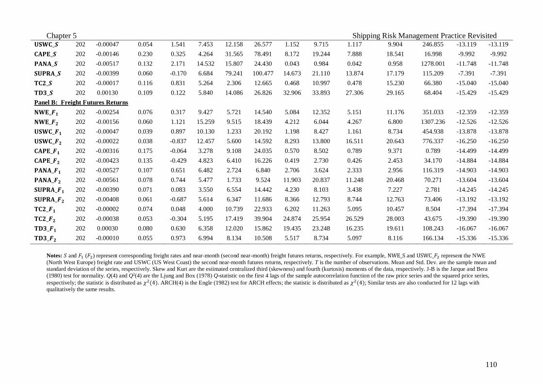
Chapter 5 Shipping Risk Management Practice Revisited
110
Notes: 𝑆 and 𝐹1 (𝐹2) represent corresponding freight rates and near-month (second near-month) freight futures returns, respectively. For example, NWE_S and USWC_𝐹2 represent the NWE
(North West Europe) freight rate and USWC (US West Coast) the second near-month futures returns, respectively. T is the number of observations. Mean and Std. Dev. are the sample mean and
standard deviation of the series, respectively. Skew and Kurt are the estimated centralized third (skewness) and fourth (kurtosis) moments of the data, respectively. J-B is the Jarque and Bera
(1980) test for normality. Q(4) and Q2(4) are the Ljung and Box (1978) Q-statistic on the first 4 lags of the sample autocorrelation function of the raw price series and the squared price series,
respectively; the statistic is distributed as 𝜒2(4). ARCH(4) is the Engle (1982) test for ARCH effects; the statistic is distributed as 𝜒2(4); Similar tests are also conducted for 12 lags with
qualitatively the same results.
𝐔𝐒𝐖𝐂_𝑺 202 -0.00047 0.054 1.541 7.453 12.158 26.577 1.152 9.715 1.117 9.904 246.855 -13.119 -13.119
𝐂𝐀𝐏𝐄_𝑺 202 -0.00146 0.230 0.325 4.264 31.565 78.491 8.172 19.244 7.888 18.541 16.998 -9.992 -9.992
𝐏𝐀𝐍𝐀_𝑺 202 -0.00517 0.132 2.171 14.532 15.807 24.430 0.043 0.984 0.042 0.958 1278.001 -11.748 -11.748
𝐒𝐔𝐏𝐑𝐀_𝑺 202 -0.00399 0.060 -0.170 6.684 79.241 100.477 14.673 21.110 13.874 17.179 115.209 -7.391 -7.391
𝐓𝐂𝟐_𝑺 202 -0.00017 0.116 0.831 5.264 2.306 12.665 0.468 10.997 0.478 15.230 66.380 -15.040 -15.040
𝐓𝐃𝟑_𝑺 202 0.00130 0.109 0.122 5.840 14.086 26.826 32.906 33.893 27.306 29.165 68.404 -15.429 -15.429
Panel B: Freight Futures Returns
𝐍𝐖𝐄_𝑭𝟏 202 -0.00254 0.076 0.317 9.427 5.721 14.540 5.084 12.352 5.151 11.176 351.033 -12.359 -12.359
𝐍𝐖𝐄_𝑭𝟐 202 -0.00156 0.060 1.121 15.259 9.515 18.439 4.212 6.044 4.267 6.800 1307.236 -12.526 -12.526
𝐔𝐒𝐖𝐂_𝑭𝟏 202 -0.00047 0.039 0.897 10.130 1.233 20.192 1.198 8.427 1.161 8.734 454.938 -13.878 -13.878
𝐔𝐒𝐖𝐂_𝑭𝟐 202 -0.00022 0.038 -0.837 12.457 5.600 14.592 8.293 13.800 16.511 20.643 776.337 -16.250 -16.250
𝐂𝐀𝐏𝐄_𝑭𝟏 202 -0.00316 0.175 -0.064 3.278 9.108 24.035 0.570 8.502 0.789 9.371 0.789 -14.499 -14.499
𝐂𝐀𝐏𝐄_𝑭𝟐 202 -0.00423 0.135 -0.429 4.823 6.410 16.226 0.419 2.730 0.426 2.453 34.170 -14.884 -14.884
𝐏𝐀𝐍𝐀_𝑭𝟏 202 -0.00527 0.107 0.651 6.482 2.724 6.840 2.706 3.624 2.333 2.956 116.319 -14.903 -14.903
𝐏𝐀𝐍𝐀_𝑭𝟐 202 -0.00561 0.078 0.744 5.477 1.733 9.524 11.903 20.837 11.248 20.468 70.271 -13.604 -13.604
𝐒𝐔𝐏𝐑𝐀_𝑭𝟏 202 -0.00390 0.071 0.083 3.550 6.554 14.442 4.230 8.103 3.438 7.227 2.781 -14.245 -14.245
𝐒𝐔𝐏𝐑𝐀_𝑭𝟐 202 -0.00408 0.061 -0.687 5.614 6.347 11.686 8.366 12.793 8.744 12.763 73.406 -13.192 -13.192
𝐓𝐂𝟐_𝑭𝟏 202 -0.00002 0.074 0.048 4.000 10.739 22.933 6.202 11.263 5.095 10.457 8.504 -17.394 -17.394
𝐓𝐂𝟐_𝑭𝟐 202 -0.00038 0.053 -0.304 5.195 17.419 39.904 24.874 25.954 26.529 28.003 43.675 -19.390 -19.390
𝐓𝐃𝟑_𝑭𝟏 202 0.00030 0.080 0.630 6.358 12.020 15.862 19.435 23.248 16.235 19.611 108.243 -16.067 -16.067
𝐓𝐃𝟑_𝑭𝟐 202 -0.00010 0.055 0.973 6.994 8.134 10.508 5.517 8.734 5.097 8.116 166.134 -15.336 -15.336

Chapter 5 Shipping Risk Management Practice Revisited
111
Table 5.2 Correlations between Weekly Logarithm of Freight Rates and Freight Futures
Panel A: Freight Rates
𝐍𝐖𝐄_𝐒 𝐔𝐒𝐖𝐂_𝑺 𝐂𝐀𝐏𝐄_𝑺 𝐏𝐀𝐍𝐀_𝑺 𝐒𝐔𝐏𝐑𝐀_𝑺 𝐓𝐂𝟐_𝑺 𝐓𝐃𝟑_𝑺
𝐍𝐖𝐄_𝐒 1
𝐔𝐒𝐖𝐂_𝑺 0.417 1
𝐂𝐀𝐏𝐄_𝑺 0.025 -0.101 1
𝐏𝐀𝐍𝐀_𝑺 -0.102 -0.105 0.329 1
𝐒𝐔𝐏𝐑𝐀_𝑺 -0.057 -0.138 0.250 0.519 1
𝐓𝐂𝟐_𝑺 0.053 0.032 0.016 -0.066 -0.022 1
𝐓𝐃𝟑_𝑺 -0.087 -0.117 0.104 0.136 0.071 -0.011 1
Panel B: Freight Rates and Near-month Futures
𝐍𝐖𝐄_𝐒 𝐔𝐒𝐖𝐂_𝑺 𝐂𝐀𝐏𝐄_𝑺 𝐏𝐀𝐍𝐀_𝑺 𝐒𝐔𝐏𝐑𝐀_𝑺 𝐓𝐂𝟐_𝑺 𝐓𝐃𝟑_𝑺
𝐍𝐖𝐄_𝑭𝟏 0.314 0.179 -0.066 -0.071 -0.027 -0.028 -0.149
𝐔𝐒𝐖𝐂_𝑭𝟏 0.081 0.382 -0.115 -0.011 -0.080 0.032 -0.094
𝐂𝐀𝐏𝐄_𝑭𝟏 0.091 0.015 0.641 0.198 0.098 -0.010 0.084
𝐏𝐀𝐍𝐀_𝑭𝟏 -0.080 -0.071 0.298 0.548 0.181 -0.049 0.076
𝐒𝐔𝐏𝐑𝐀_𝑭𝟏 -0.121 -0.119 0.237 0.433 0.476 -0.028 0.050
𝐓𝐂𝟐_𝑭𝟏 0.076 0.031 -0.036 -0.035 -0.050 0.520 0.099
𝐓𝐃𝟑_𝑭𝟏 0.035 -0.035 0.056 0.136 0.045 -0.082 0.641
Panel C: Freight Rates and Second near-month Futures
𝐍𝐖𝐄_𝐒 𝐔𝐒𝐖𝐂_𝑺 𝐂𝐀𝐏𝐄_𝑺 𝐏𝐀𝐍𝐀_𝑺 𝐒𝐔𝐏𝐑𝐀_𝑺 𝐓𝐂𝟐_𝑺 𝐓𝐃𝟑_𝑺
𝐍𝐖𝐄_𝑭𝟐 0.223 0.122 -0.010 -0.134 -0.142 -0.005 -0.075
𝐔𝐒𝐖𝐂_𝑭𝟐 0.073 0.244 -0.118 -0.082 -0.120 0.081 -0.095

Chapter 5 Shipping Risk Management Practice Revisited
112
Notes: See the notes to Table 5.1 for the definitions of the variables.
𝐂𝐀𝐏𝐄_𝑭𝟐 -0.011 0.011 0.493 0.106 0.066 -0.014 -0.011
𝐏𝐀𝐍𝐀_𝑭𝟐 -0.081 -0.050 0.291 0.464 0.133 -0.066 0.027
𝐒𝐔𝐏𝐑𝐀_𝑭𝟐 -0.198 -0.066 0.235 0.377 0.355 -0.027 -0.037
𝐓𝐂𝟐_𝑭𝟐 -0.013 -0.045 -0.012 -0.009 -0.036 0.284 0.094
𝐓𝐃𝟑_𝑭𝟐 -0.049 -0.059 0.130 0.204 0.039 -0.084 0.524

Chapter 5 Shipping Risk Management Practice Revisited
113
5.4. Empirical Results
Both in-sample and out-of-sample tests are performed to investigate the performance of the
well-diversified portfolio comprising physical freight rates, as well as the direct hedge and
cross hedge portfolios also comprising freight futures. In-sample tests are performed from
February 2011 to April 2015 based on a total of 202 observations (weekly), while weekly
rolling out-of-sample tests are conducted from April 2015 to June 2016 based on 60
observations.
5.4.1. Performance of well-diversified portfolio of freight rates
Due to the negative correlations between the container, dry-bulk, and tanker freight rates, as
seen in Table 5.2, we investigate if shipping market practitioners can minimise their freight
rate exposure through holding a well-diversified portfolio of freight routes. The VR and UI of
the well-diversified portfolio, over and above an equally weighted portfolio of freight rates,
are presented in Table 5.3.57 In-sample and out-of-sample tests are reported in Panels A and
B, respectively. The results indicate that there is a significant decrease in the variance of the
well-diversified portfolio relative to an equally weighted portfolio in all the scenarios
examined. In-sample and out-of-sample tests suggest that the well-diversified portfolio
reduces freight rate risks between 28–48% and 32–48%, respectively, except scenario 6. 58
The well-diversified portfolio for the base scenario, comprising freight rates in all three sub-
sectors, produces a VR out-of-sample of up to 42%. Moreover, we document a utility increase
in all scenarios (except again in scenario 6 for out-of-sample observations) for the well-
diversified portfolio. Overall, the findings suggest that the traditional freight rate risk
management through portfolio diversification can be an effective risk management solution.
57 An equally weight portfolio of freight rates is used as a benchmark. 58 Scenario 6, TC2 and TD3 freight rate routes produce very low correlation, as presented in Table 5.2. This results in no
effective reduction of variance through diversification.

Chapter 5 Shipping Risk Management Practice Revisited
114
Table 5.3 Performance of Well-Diversified Portfolio of Freight Rates
Notes: 𝜎𝐸𝑊2 (𝜎𝑊𝐷
2 ) and 𝑈𝐸𝑊 (𝑈𝑊𝐷) denote the variances and utilities of an equally weighted (well-diversified) portfolio of
freight rates, respectively. 𝑈𝐸𝑊 and 𝑈𝑊𝐷 are calculated for the coefficient of risk aversion (k) equal to 1. 𝑉𝑅𝑊𝐷_𝐸𝑊 and
𝑈𝐼𝑊𝐷_𝐸𝑊 are the variance reduction (VR) and utility increase (UI) of the well-diversified portfolio with respect to an equally
weighted portfolio of freight rates.
5.4.2. Performance of direct hedge portfolio
Results for in-sample and out-of-sample VR (and UI) for both near-month and second near-
month freight futures contracts are presented in Tables 5.4 (along with Table 5.4 cont.),
respectively. In the container USWC route, the time-varying and naïve hedge ratio seem to
produce the highest VR of 10.88% (4.48%) and 21.33% (12.50%) for in-sample and out-of-
sample near-month (second near-month) freight futures, respectively. The opposite is found
for the container NWE route, with the time-varying VECM-GARCH model outperforming
all other specifications, with a VR of 10.30% (10.16%) and 10.10% (3.02%) for in-sample
and out-of-sample near-month (second near-month) freight futures, respectively. 59 Overall,
near-month freight futures perform better than second near-month freight futures for the
container sub-sector. This may be attributed to an increase in last minute trading activity on
59 Except for second near-month NWE futures contracts, where the conventional OLS model generates the highest VR of
10.77%
Base
Scenario
Scenario 1 Scenario 2 Scenario 3 Scenario 4 Scenario 5 Scenario 6
Panel A: In-Sample Performance
𝝈𝑬𝑾𝟐 0.05612 0.07070 0.07434 0.06002 0.09011 0.11049 0.07767
𝝈𝑾𝑫𝟐 0.03320 0.03699 0.04821 0.04324 0.05425 0.05974 0.07754
𝑽𝑹𝑾𝑫_𝑬𝑾 40.84% 47.68% 35.16% 27.96% 39.80% 45.93% 0.17%
𝑼𝑬𝑾 -0.00535 -0.00831 -0.00742 -0.00480 -0.01108 -0.01575 -0.00547
𝑼𝑾𝑫 -0.00267 -0.00349 -0.00469 -0.00197 -0.00349 -0.00756 -0.00540
𝑼𝑰𝑾𝑫_𝑬𝑾 0.00268 0.00482 0.00274 0.00282 0.00759 0.00819 0.00006
Panel B: Out-of-Sample Performance
𝝈𝑬𝑾𝟐 0.06194 0.07911 0.07658 0.07279 0.12401 0.11110 0.08191
𝝈𝑾𝑫𝟐 0.03626 0.04147 0.04874 0.04928 0.06802 0.05950 0.08168
𝑽𝑹𝑾𝑫_𝑬𝑾 41.49% 47.61% 36.35% 32.25% 45.03% 46.45% 0.27%
𝑼𝑬𝑾 -0.00598 -0.00923 -0.00762 -0.00693 -0.01878 -0.01520 -0.00682
𝑼𝑾𝑫 -0.00365 -0.00468 -0.00499 -0.00365 -0.00669 -0.00737 -0.00685
𝑼𝑰𝑾𝑫_𝑬𝑾 0.00233 0.00455 0.00263 0.00328 0.01209 0.00783 -0.00004

Chapter 5 Shipping Risk Management Practice Revisited
115
the back of more market information typically incorporated in near-month futures contracts
approaching maturity compared to second near-month contracts. Further, the USWC freight
futures perform better than the NWE freight futures (for out-of-sample analysis), reflected in
the higher freight rate variance of the latter route. This may be driven by the lower number of
liner services in the Shanghai–US route, pointing to a more stable freight rate environment in
this case.60
In-sample tests for the dry-bulk sub-sector suggest that the conventional OLS model
generates the highest hedging effectiveness for Capesize and Panamax freight futures, with a
VR of 38.13% (22.76%) and 31.20% (23.48%) for near-month (second near-month) freight
futures, respectively. In contrast, for Supramax freight futures, the VECM-GARCH model
exhibits the highest VR of 19.25% (14.62%) for near-month (second near-month) freight
futures contracts. Out-of-sample tests suggest that the VECM-GARCH (VECM) model
produces the highest VR of 33.48% (13.38%) for near-month (second near-month) Supramax
freight futures. Further, a naïve hedge ratio model performs better for Capesize freight rates
with a VR of 47.51% (27.44%) for near-month (second near-month) freight futures contracts.
Panamax freight futures generate highest hedging effectiveness using an OLS (VECM-
GARCH) model for near-month (second near-month) contracts with a VR of 21.91%
(10.26%). Overall, the Capesize freight futures have the highest performance due to their
higher liquidity in terms of trading volume. It appears that similar to container futures, near-
month dry-bulk freight futures perform better than second near-month freight futures.
A time-varying hedge ratio using a VECM-GARCH model generates the highest hedging
effectiveness for in-sample analysis with tanker freight futures contracts, with a VR of
27.52% (10.04%) and 48.22% (32.47%) for near-month (second near-month) TC2 and TD3
futures contracts, respectively. In contrast, constant hedge ratios perform better for out-of-
sample analysis, with a VR of as high as 29.17% (19.03%) and 34.31% (23.45%) for near-
month (second near-month) TC2 and TD3 futures contracts, respectively. TD3 freight futures
contracts perform better than TC2 freight futures contracts.
In general, the results suggest that the VR for all models and across all different freight
futures is relatively low, with an average of around 20%. In addition, all freight futures prices
seem to follow a martingale process, with the MVHR equal to the UMHR for all coefficients
60 During the sample period (2011–2016), Europe imported on average 34 million TEU containers annually, whereas the US
imported on average only 21 million.
Chapter 5 Shipping Risk Management Practice Revisited
116
of risk aversion. This limits the usefulness of freight futures contracts for
investment/speculative purposes, which could be attributed to the low market liquidity,
creating sticky (stale) prices. Thus, the UI criterion is estimated only for the case of the risk-
neutral (k = 1) participant as a measure of the increase of the utility function due to hedging.
In-sample tests indicate that both the OLS and VECM-GARCH models perform similarly,
whereas out-of-sample tests indicate that the OLS model performs best in most scenarios.
Finally, we investigate if the risks associated with the well-diversifying portfolio of physical
freight rates are further reduced when using freight futures. To this end, freight futures
contracts are added to the well-diversified portfolio, where the weights of these futures
contracts are estimated using the MVHR of Equation (3) (see Portfolio 2, Constraint C, in
Section 5.2). The decision to keep the weights of the physical freight rates unchanged, while
hedging the freight rate exposure, is motivated by the fact that practitioners tend to use open
positions in the physical freight market by considering the risk-return trade-off of this market,
rather than that of the freight derivatives market.

Chapter 5 Shipping Risk Management Practice Revisited
117
Table 5.4 Direct Hedge Performance: In-sample Tests
Near-Month Contracts Second Near-Month Contracts
Container Dry Bulk Tanker Container Dry Bulk Tanker
NWE_1 USWC_1 CAPE_1 PANA_1 SUPRA_1 TC2_1 TD3_1 NWE_2 USWC_2 CAPE_2 PANA_2 SUPRA_2 TC2_2 TD3_2
Panel 1a: Minimum Variance Hedge Ratio – MVHR
Naïve 1 1 1 1 1 1 1 1 1 1 1 1 1 1
OLS 0.54 0.45 0.81 0.69 0.36 0.80 0.95 0.85 0.29 0.82 0.82 0.34 0.53 1.10
VECM 0.51 0.45 0.81 0.73 0.39 0.87 0.95 0.85 0.27 0.87 0.91 0.38 0.74 1.08
VECM-GARCH - - - - - - - - - - - - - -
Panel 1b: Variance of Hedged Portfolio
Unhedged 0.02432 0.00295 0.05313 0.01733 0.00357 0.01345 0.01195 0.02432 0.00295 0.05313 0.01733 0.00357 0.01345 0.01195
Naïve 0.02379 0.00311 0.03384 0.01304 0.00493 0.00996 0.00626 0.02179 0.00357 0.04168 0.01346 0.00475 0.01276 0.00831
OLS 0.02260 0.00264 0.03287 0.01192 0.00289 0.00975 0.00624 0.02170 0.00282 0.04104 0.01326 0.00313 0.01234 0.00828
VECM 0.02261 0.00264 0.03287 0.01194 0.00289 0.00977 0.00624 0.02170 0.00282 0.04110 0.01331 0.00313 0.01238 0.00829
VECM-GARCH 0.02182 0.00263 0.03291 0.01196 0.00288 0.00975 0.00619 0.02185 0.00282 0.03972 0.01326 0.00305 0.01210 0.00807
Panel 1c: Variance Reduction – VR
Naïve 2.19% -5.48% 36.31% 24.76% -38.17% 25.97% 47.62% 10.42% -20.98% 21.56% 22.34% -32.99% 5.08% 30.45%
OLS 7.09% 10.43% 38.13%* 31.20%* 19.00% 27.54% 47.76% 10.77%* 4.20% 22.76% 23.48%* 12.39% 8.21% 30.68%
VECM 7.06% 10.43% 38.13% 31.08% 18.92% 27.34% 47.76% 10.77% 4.17% 22.63% 23.18% 12.20% 7.92% 30.67%
VECM-GARCH 10.30%* 10.88%* 38.05% 31.02% 19.25%* 27.52%* 48.22%* 10.16% 4.48%* 25.24%* 23.47% 14.62%* 10.04%* 32.47%*
Panel 2a: Expected Utility (k = 1)
Unhedged -0.02953 -0.00328 -0.05539 -0.02290 -0.00782 -0.01432 -0.01107 -0.02953 -0.00328 -0.05539 -0.02290 -0.00782 -0.01432 -0.01107
Naïve -0.02633 -0.00298 -0.03101 -0.01289 -0.00478 -0.01096 -0.00512 -0.02533 -0.00368 -0.03909 -0.01313 -0.00469 -0.01412 -0.00709
OLS -0.02636 -0.00277 -0.03106 -0.01357 -0.00555 -0.01075 -0.00512 -0.02550 -0.00310 -0.03939 -0.01400 -0.00592 -0.01354 -0.00703
VAR -0.02646 -0.00277 -0.03103 -0.01336 -0.00546 -0.01078 -0.00512 -0.02549 -0.00310 -0.03917 -0.01352 -0.00576 -0.01365 -0.00704
VAR-GARCH -0.02383 -0.00285 -0.03134 -0.01316 -0.00548 -0.01047 -0.00480 -0.02400 -0.00334 -0.03984 -0.01386 -0.00515 -0.01194 -0.00754
Panel 2b: Utility Increase – UI (k = 1)
Naïve 0.00320 0.00030 0.02437* 0.01001* 0.00304* 0.00336 0.00594 0.00420 -0.00040 0.01629* 0.00977* 0.00313* 0.00021 0.00397
OLS 0.00317 0.00051 0.02433 0.00933 0.00227 0.00357 0.00594 0.00403 0.00018* 0.01600 0.00890 0.00190 0.00078 0.00404*
VAR 0.00307 0.00052* 0.02436 0.00955 0.00236 0.00355 0.00594 0.00404 0.00018 0.01622 0.00939 0.00206 0.00068 0.00403

Chapter 5 Shipping Risk Management Practice Revisited
118
VAR-GARCH 0.00570* 0.00043 0.02405 0.00974 0.00234 0.00385* 0.00626* 0.00553* -0.00006 0.01555 0.00904 0.00267 0.00238* 0.00353
Table 5.4 Direct Hedge Performance: Out-of-sample Tests
Near-Month Contracts Second Near-Month Contracts
Container Dry Bulk Tanker Container Dry Bulk Tanker
NWE_1 USWC_1 CAPE_1 PANA_1 SUPRA_1 TC2_1 TD3_1 NWE_2 USWC_2 CAPE_2 PANA_2 SUPRA_2 TC2_2 TD3_2
Panel 1a: Variance of Hedged Portfolio
Unhedged 0.18372 0.01811 0.09001 0.00852 0.00429 0.00935 0.04127 0.18372 0.01811 0.09001 0.00852 0.00429 0.00935 0.04127
Naïve 0.15919 0.01425 0.04725 0.00975 0.00378 0.00701 0.02711 0.17899 0.01585 0.06531 0.00955 0.00522 0.00772 0.03184
OLS 0.16568 0.01548 0.04773 0.00666 0.00289 0.00663 0.02730 0.17962 0.01704 0.06600 0.00786 0.00372 0.00769 0.03159
VECM 0.16562 0.01525 0.04741 0.00681 0.00290 0.00671 0.02725 0.17976 0.01701 0.06563 0.00827 0.00372 0.00757 0.03160
VECM-GARCH 0.16517 0.01557 0.04769 0.00693 0.00286 0.00678 0.02935 0.17816 0.01674 0.06671 0.00765 0.00377 0.00778 0.03216
Panel 1b: Variance Reduction – VR
Naïve 13.35% 21.33%* 47.51%* -14.43% 12.00% 25.10% 34.31%* 2.58% 12.50%* 27.44%* -12.04% -21.48% 17.50% 22.84%
OLS 9.82% 14.55% 46.98% 21.91%* 32.68% 29.17%* 33.85% 2.23% 5.90% 26.67% 7.83% 13.37% 17.84% 23.45%*
VECM 9.85% 15.81% 47.33% 20.12% 32.56% 28.32% 33.97% 2.16% 6.09% 27.09% 3.00% 13.38%* 19.03%* 23.44%
VECM-GARCH 10.10%* 14.01% 47.02% 18.70% 33.48%* 27.56% 28.88% 3.02%* 7.55% 25.89% 10.26%* 12.15% 16.86% 22.08%
Panel 2a: Expected Utility (k = 1)
Unhedged -0.17483 -0.03091 -0.08335 -0.01001 -0.00528 -0.01744 -0.05204 -0.17483 -0.03091 -0.08335 -0.01001 -0.00528 -0.01744 -0.05204
Naïve -0.14284 -0.01573 -0.04443 -0.00908 -0.00361 -0.00825 -0.02999 -0.16000 -0.01696 -0.06221 -0.01051 -0.00498 -0.01073 -0.03504
OLS -0.15213 -0.02249 -0.04369 -0.00653 -0.00390 -0.00923 -0.02985 -0.16179 -0.02608 -0.06252 -0.00897 -0.00444 -0.01241 -0.03339
VECM -0.15190 -0.02190 -0.04347 -0.00660 -0.00363 -0.00888 -0.02983 -0.16156 -0.02614 -0.06247 -0.00938 -0.00435 -0.01178 -0.03342
VAR-GARCH -0.15087 -0.02109 -0.04386 -0.00533 -0.00426 -0.00906 -0.03175 -0.14977 -0.02228 -0.06449 -0.00908 -0.00407 -0.01096 -0.03513
Panel 2b: Utility Increase – UI (k = 1)
Naïve 0.03199* 0.01518* 0.03891 0.00092 0.00166* 0.00919* 0.02205 0.01483 0.01395* 0.02114* -0.00050 0.00029 0.00671* 0.01699
OLS 0.02270 0.00842 0.03966 0.00347 0.00137 0.00821 0.02219 0.01305 0.00483 0.02083 0.00104* 0.00083 0.00503 0.01865*
VECM 0.02294 0.00901 0.03987* 0.00341 0.00164 0.00856 0.02220* 0.01327 0.00477 0.02088 0.00062 0.00093 0.00566 0.01862
VECM-GARCH 0.02397 0.00982 0.03949 0.00467* 0.00102 0.00838 0.02029 0.02507* 0.00863 0.01886 0.00092 0.00121* 0.00648 0.01691
Notes: NWE_1 and NWE_2 are the NWE container freight routes hedged with corresponding near-month and second near-month freight futures, respectively. Similarly, USWC_1 (USWC_2),
CAPE_1 (CAPE_2), PANA_1 (PANA_2), SUPRA_1 (SUPRA_2), TC2_1 (TC2_2) and TD3_1 (TD3_2) are USWC, Capesize, Panamax, Supramax, TC2 and TD3 freight routes hedged with
corresponding near- (second near-) month freight futures contracts, respectively. * denotes the model with the highest variance reduction (VR) and utility increase (UI) per hedge model. k is the
coefficient of risk aversion.

Chapter 5 Shipping Risk Management Practice Revisited
119

Chapter 5 Tracing Lead-lag Relationships between Commodities and Freights
120
Table 5.5 presents the VR and UI of the direct hedge portfolio over and above the well-
diversified portfolio of freight rates, for both in-sample and out-of-sample tests, Equations
(19) and (20). Results indicate that the direct hedge portfolio using freight futures further
decrease the freight rate risk associated with the well-diversified portfolio of freight rates up
to as high as 17.52% (observed in the out-of-sample analysis for scenario 6). We also observe
that the UI for all the scenarios are positive indicating that use of freight futures contracts
with a direct hedge approach increases the satisfaction level of the hedgers in addition to the
traditional optimal diversification. Further, near-month freight futures contracts produce
higher VR as compared to second near-month futures contracts. Overall, the models in-
sample and out-of-sample perform similarly, with the highest VR observed in Scenario 6.
This indicates that market participants with a mixed portfolio of tanker freight rate routes will
receive the highest risk minimisation through freight futures hedging.
Table 5.5 Direct Hedge vs. Well-diversified Portfolio Performance
Base Scenario 1 Scenario 2 Scenario 3 Scenario 4 Scenario 5 Scenario 6

Chapter 5 Tracing Lead-lag Relationships between Commodities and Freights
121
Notes: 𝜎𝐷𝐻,12 (𝑈𝐷𝐻,1) and 𝜎𝐷𝐻,2
2 (𝑈𝐷𝐻,2) are the variances (utilities) of the near-month and second near-month returns of the
direct hedge portfolios, respectively. 𝑉𝑅𝐷𝐻_𝑊𝐷,1 (𝑈𝐼𝐷𝐻_𝑊𝐷,1) and 𝑉𝑅𝐷𝐻_𝑊𝐷,2 (𝑈𝐼𝐷𝐻_𝑊𝐷,2) are the VR and UI of the direct
hedge over and above the well-diversified portfolio. See the notes to Table 5.3 for the definitions of the other variables.
5.4.3. Performance of cross hedge portfolio
As the last step, we estimate a cross-hedge portfolio of freight futures to hedge the risks
associated with the well-diversified portfolio of physical freight rates without changing the
weights of the freight rates within the latter portfolio.61 Similar to the previous section, VR
and UI are used as measures of hedging performance of the cross hedge portfolio over and
above the well-diversified portfolio of freight rates. The results presented in Table 5.6
indicate that the cross hedge portfolio using freight futures can further reduce the risks
associated with the well-diversified portfolio of freight rates. The results are qualitatively
similar both in-sample and out-of-sample.62 Further, near-month futures contracts generate
higher hedging effectiveness than second-month futures contracts. Similar to the direct hedge
61 Details of the freight rate weights of the cross hedge portfolios are presented in Section5.2. 62 Following a comment by a reviewer, we have replicated the cross hedge analysis again with only dry-bulk and tanker
futures’ contracts (without including container futures). The results suggest that for several scenarios, including container
futures yields higher variance reductions, which is consistent with the view that including this segment adds value to the
strategy.
Scenario
Panel A: In-Sample Performance
𝝈𝑾𝑫𝟐 0.03320 0.03699 0.04821 0.04324 0.05425 0.05974 0.07754
𝝈𝑫𝑯,𝟏𝟐 0.02978 0.03395 0.04335 0.03793 0.05135 0.05379 0.06497
𝑽𝑹𝑫𝑯_𝑾𝑫,𝟏 10.31% 8.23% 10.08% 12.28% 5.34% 9.97% 16.21%
𝝈𝑫𝑯,𝟐𝟐 0.03114 0.03489 0.04581 0.04088 0.05308 0.05600 0.07259
𝑽𝑹𝑫𝑯_𝑾𝑫,𝟐 6.20% 5.70% 4.98% 5.45% 2.14% 6.26% 6.38%
𝑼𝑾𝑫 -0.00267 -0.00349 -0.00469 -0.00197 -0.00349 -0.00756 -0.00540
𝑼𝑫𝑯,𝟏 -0.00185 -0.00247 -0.00338 -0.00145 -0.00295 -0.00546 -0.00375
𝑼𝑰𝑫𝑯_𝑾𝑫,𝟏 0.00083 0.00102 0.00131 0.00052 0.00053 0.00210 0.00165
𝑼𝑫𝑯,𝟐 -0.00194 -0.00261 -0.00352 -0.00168 -0.00328 -0.00573 -0.00451
𝑼𝑰𝑫𝑯_𝑾𝑫,𝟐 0.00073 0.00088 0.00117 0.00029 0.00021 0.00182 0.00090
Panel B: Out-of-Sample Performance
𝝈𝑾𝑫𝟐 0.03626 0.04147 0.04874 0.04928 0.06802 0.05950 0.08168
𝝈𝑫𝑯,𝟏𝟐 0.03281 0.03813 0.04324 0.04343 0.06390 0.05311 0.06736
𝑽𝑹𝑫𝑯_𝑾𝑫,𝟏 9.50% 8.04% 11.27% 11.73% 5.89% 10.70% 17.52%
𝝈𝑫𝑯,𝟐𝟐 0.03468 0.03932 0.04607 0.04719 0.06593 0.05573 0.07541
𝑽𝑹𝑫𝑯_𝑾𝑫,𝟐 4.01% 4.83% 5.42% 3.68% 2.40% 6.29% 7.56%
𝑼𝑾𝑫 -0.00365 -0.00468 -0.00499 -0.00365 -0.00669 -0.00737 -0.00685
𝑼𝑫𝑯,𝟏 -0.00231 -0.00302 -0.00346 -0.00232 -0.00482 -0.00514 -0.00466
𝑼𝑰𝑫𝑯_𝑾𝑫,𝟏 0.00134 0.00166 0.00153 0.00133 0.00186 0.00223 0.00220
𝑼𝑫𝑯,𝟐 -0.00261 -0.00335 -0.00378 -0.00287 -0.00554 -0.00556 -0.00574
𝑼𝑰𝑫𝑯_𝑾𝑫,𝟐 0.00103 0.00133 0.00121 0.00078 0.00115 0.00181 0.00111

Chapter 5 Tracing Lead-lag Relationships between Commodities and Freights
122
portfolio, the UI of the cross hedge portfolio over and above the well-diversified portfolio is
positive for all the scenarios.

Chapter 5 Tracing Lead-lag Relationships between Commodities and Freights
123
Table 5.6 Cross Hedge vs. Well-diversified Portfolio Performance
Base
Scenario
Scenario 1 Scenario 2 Scenario 3 Scenario 4 Scenario 5 Scenario 6
Panel A: In-Sample Performance
𝝈𝑾𝑫𝟐 0.03320 0.03699 0.04821 0.04324 0.05425 0.05974 0.07754
𝝈𝑪𝑯,𝟏𝟐 0.02954 0.03356 0.04319 0.03789 0.05092 0.05375 0.06450
𝑽𝑹𝑪𝑯_𝑾𝑫,𝟏 11.01% 9.29% 10.41% 12.38% 6.14% 10.02% 16.82%
𝝈𝑪𝑯,𝟐𝟐 0.03073 0.03420 0.04572 0.04070 0.05234 0.05584 0.07223
𝑽𝑹𝑪𝑯_𝑾𝑫,𝟐 7.45% 7.54% 5.16% 5.88% 3.50% 6.53% 6.84%
𝑼𝑾𝑫 -0.00267 -0.00349 -0.00469 -0.00197 -0.00349 -0.00756 -0.00540
𝑼𝑪𝑯,𝟏 -0.00184 -0.00244 -0.00340 -0.00138 -0.00277 -0.00547 -0.00366
𝑼𝑰𝑪𝑯_𝑾𝑫,𝟏 0.00084 0.00105 0.00128 0.00059 0.00072 0.00209 0.00174
𝑼𝑪𝑯,𝟐 -0.00178 -0.00236 -0.00364 -0.00140 -0.00255 -0.00572 -0.00445
𝑼𝑰𝑪𝑯_𝑾𝑫,𝟐 0.00089 0.00113 0.00105 0.00058 0.00094 0.00184 0.00095
Panel B: Out-of-Sample Performance
𝝈𝑾𝑫𝟐 0.03626 0.04147 0.04874 0.04928 0.06802 0.05950 0.08168
𝝈𝑪𝑯,𝟏𝟐 0.03268 0.03796 0.04313 0.04328 0.06362 0.05309 0.06682
𝑽𝑹𝑪𝑯_𝑾𝑫,𝟏 9.87% 8.47% 11.49% 12.02% 6.29% 10.75% 18.19%
𝝈𝑪𝑯,𝟐𝟐 0.03455 0.03918 0.04604 0.04714 0.06597 0.05566 0.07509
𝑽𝑹𝑪𝑯_𝑾𝑫,𝟐 4.80% 5.62% 5.54% 4.31% 3.00% 6.45% 8.06%
𝑼𝑾𝑫 -0.00365 -0.00468 -0.00499 -0.00365 -0.00669 -0.00737 -0.00685
𝑼𝑪𝑯,𝟏 -0.00241 -0.00307 -0.00348 -0.00230 -0.00456 -0.00513 -0.00456

Chapter 5 Tracing Lead-lag Relationships between Commodities and Freights
124
Notes: 𝜎𝐶𝐻,12 (𝑈𝐶𝐻,1) and 𝜎𝐶𝐻,2
2 (𝑈𝐶𝐻,2) are the variances (utilities) of the near-month and second near-month returns of the
cross hedge portfolios, respectively. 𝑉𝑅𝐶𝐻_𝑊𝐷,1 (𝑈𝐼𝐶𝐻_𝑊𝐷,1) and 𝑉𝑅𝐶𝐻_𝑊𝐷,2 (𝑈𝐼𝐶𝐻_𝑊𝐷,2) are the VR and UI of the cross
hedge over and above the well-diversified portfolio. See the notes to Table 5.3 for the definitions of the other variables.
A comparative analysis of the cross hedge and the direct hedge portfolios is also performed,
based on the VR and UI criteria calculated from Equations (21) and (22), respectively. The
weights of the physical freight rates in both portfolios are the same as in the well-diversified
portfolio of freight rates, as shown in Constraints C and D (in Section 5.2). In-sample and
out-of-sample tests are presented in Table 5.7, indicating that the cross hedge portfolio
marginally outperforms the direct hedge portfolio by reducing the variance of the portfolio up
to 1.96% (for in-sample analysis in Scenario 1).
𝑼𝑰𝑪𝑯_𝑾𝑫,𝟏 0.00124 0.00161 0.00151 0.00135 0.00213 0.00224 0.00229
𝑼𝑪𝑯,𝟐 -0.00272 -0.00340 -0.00389 -0.00275 -0.00505 -0.00555 -0.00565
𝑼𝑰𝑪𝑯_𝑾𝑫,𝟐 0.00093 0.00127 0.00110 0.00090 0.00163 0.00182 0.00121

Chapter 5 Tracing Lead-lag Relationships between Commodities and Freights
125
Table 5.7 Cross Hedge vs. Direct Hedge Portfolio Performance
Base
Scenario
Scenario 1 Scenario 2 Scenario 3 Scenario 4 Scenario 5 Scenario 6
Panel A: In-Sample Performance
𝝈𝑫𝑯,𝟏𝟐 0.02978 0.03395 0.04335 0.03793 0.05135 0.05379 0.06497
𝝈𝑪𝑯,𝟏𝟐 0.02954 0.03356 0.04319 0.03789 0.05092 0.05375 0.06450
𝑽𝑹𝑪𝑯_𝑫𝑯,𝟏 0.78% 1.15% 0.38% 0.11% 0.84% 0.06% 0.73%
𝝈𝑫𝑯,𝟐𝟐 0.03114 0.03489 0.04581 0.04088 0.05308 0.05600 0.07259
𝝈𝑪𝑯,𝟐𝟐 0.03073 0.03420 0.04572 0.04070 0.05234 0.05584 0.07223
𝑽𝑹𝑪𝑯_𝑫𝑯,𝟐 1.34% 1.96% 0.19% 0.45% 1.39% 0.28% 0.49%
𝑼𝑫𝑯,𝟏 -0.00185 -0.00247 -0.00338 -0.00145 -0.00295 -0.00546 -0.00375
𝑼𝑪𝑯,𝟏 -0.00184 -0.00244 -0.00340 -0.00138 -0.00277 -0.00547 -0.00366
𝑼𝑰𝑪𝑯_𝑫𝑯,𝟏 0.00001 0.00003 -0.00002 0.00007 0.00019 -0.00001 0.00009
𝑼𝑫𝑯,𝟐 -0.00194 -0.00261 -0.00352 -0.00168 -0.00328 -0.00573 -0.00451
𝑼𝑪𝑯,𝟐 -0.00178 -0.00236 -0.00364 -0.00140 -0.00255 -0.00572 -0.00445
𝑼𝑰𝑪𝑯_𝑫𝑯,𝟐 0.00016 0.00025 -0.00012 0.00029 0.00073 0.00002 0.00005
Panel B: Out-of-Sample Performance
𝝈𝑫𝑯,𝟏𝟐 0.03281 0.03813 0.04324 0.04343 0.06390 0.05311 0.06736

Chapter 5 Tracing Lead-lag Relationships between Commodities and Freights
126
Notes: 𝑉𝑅𝐶𝐻_𝐷𝐻,1 (𝑈𝐼𝐶𝐻_𝐷𝐻,1) and 𝑉𝑅𝐶𝐻_𝐷𝐻,2 (𝑈𝐼𝐶𝐻_𝐷𝐻,2) are the VR (and UI) of the cross hedge over and above the direct
hedge portfolio, respectively. See the notes to Tables 5.5 and 5.6 for the definitions of the other variables. * denotes
significance at 99% level for out-of-sample VR.
The out-of-sample VR of the cross hedge over and above the direct hedge is found to be
statistically significant at the 99% level. This indicates that a marginal benefit of the cross
hedge with the use of futures contracts is observed over the direct hedge. Moreover, the cross
hedge portfolio performs relatively better for second near-month futures contracts compared
to near-month futures contracts. Second near-month futures contracts produce a further VR as
high as 1.96% (0.88%), whereas near-month futures contracts produce the highest VR of
1.15% (0.81%) in-sample (out-of-sample).
𝝈𝑪𝑯,𝟏𝟐 0.03268 0.03796 0.04313 0.04328 0.06362 0.05309 0.06682
𝑽𝑹𝑪𝑯_𝑫𝑯,𝟏 0.41%* 0.47%* 0.25%* 0.33%* 0.42%* 0.05%* 0.81%*
𝝈𝑫𝑯,𝟐𝟐 0.03468 0.03932 0.04607 0.04719 0.06593 0.05573 0.07541
𝝈𝑪𝑯,𝟐𝟐 0.03455 0.03918 0.04604 0.04714 0.06597 0.05566 0.07509
𝑽𝑹𝑪𝑯_𝑫𝑯,𝟐 0.88%* 0.87%* 0.14%* 0.71%* 0.63%* 0.18%* 0.60%*
𝑼𝑫𝑯,𝟏 -0.00231 -0.00302 -0.00346 -0.00232 -0.00482 -0.00514 -0.00466
𝑼𝑪𝑯,𝟏 -0.00241 -0.00307 -0.00348 -0.00230 -0.00456 -0.00513 -0.00456
𝑼𝑰𝑪𝑯_𝑫𝑯,𝟏 -0.00011 -0.00005 -0.00002 0.00002 0.00026 0.00001 0.00009
𝑼𝑫𝑯,𝟐 -0.00261 -0.00335 -0.00378 -0.00287 -0.00554 -0.00556 -0.00574
𝑼𝑪𝑯,𝟐 -0.00272 -0.00340 -0.00389 -0.00275 -0.00505 -0.00555 -0.00565
𝑼𝑰𝑪𝑯_𝑫𝑯,𝟐 -0.00009 -0.00005 -0.00019 0.00001 0.00022 -0.00028 0.00014

Chapter 5 Tracing Lead-lag Relationships between Commodities and Freights
127
5.5. Conclusion
This study develops for the first time a new portfolio approach combining the physical
diversification of freight rates and the financial hedging of freight derivatives, in three major
sub-sectors (container, tanker and dry-bulk) of the international shipping industry. It is also
the first to provide insights on the hedging performance of the recently developed container
futures market, with the underlying container segment of the shipping industry corresponding
up to 60% of the overall value of goods transported by sea. The examination of container
freight derivatives becomes relevant given the emerging nature of this market, potentially
making corporate owners and operators reluctant to utilise it for hedging their freight rate
exposures. This is reflected in its relatively low liquidity, which in turn leads to the inferior
hedging effectiveness of the container freight futures contracts relative to more mature
shipping futures markets (dry-bulk and tanker). The results point to a decrease in freight rate
risk up to 48% by holding a diversified portfolio of freight rates, and an additional decrease
of up to 8% by hedging freight rate risk with futures contracts. This study highlights that
practitioners can realise additional benefits (minimising their risk exposure) by holding
freight futures’ contracts together with a well-diversified portfolio of freight rates. The results
can also act as a yardstick for researchers to gain a better understanding of the correlations
between freight futures and underlying freight rate markets and, thus, help to improve
hedging strategies. The findings have important implications for overall business,
commercial and hedging strategies in the shipping industry, and can encourage the trading of
freight futures contracts, which can potentially lead to improvements in freight futures
markets liquidity.
Chapter 6 Conclusion
128
6. Conclusion
6.1. Summary and Concluding Remarks
This thesis provides a wide-ranging methodology and unfolds new findings in derivatives and
risk management for shipping and commodities. The work aims to investigate and explore
some of the unchartered and overlooked investment opportunities for shipowners and
charterers and provide effective risk management solutions. These risk management
strategies are developed through market anticipation (Chapter 3 and 4) and hedging market
fluctuations (Chapter 5). A strong underpinning of the research is provided by an extensive
literature review that covers the development of information transmission and hedging of
both equities and commodities (including freight) markets. This is important for readers who
do not have expertise in this specialised area, creating a path for a better understanding of the
flow of the research. The three empirical chapters (Chapters 3–5) also provide more a more
specific literature review, aiming to motivate the respective research topics.
The spillover effect between futures, options and underlying physical freight rates are
investigated in Chapter 3, which demonstrates that options contracts, despite being derivative
contracts, suffer from market liquidity and fail to react to new market information. The
results suggest that freight futures contracts absorb new market information and spill it to
freight rates, followed by freight options contracts. This provides valuable information for
investors and hedgers, who can use options contracts for generating returns and to hedge
freight rate fluctuations, respectively.
This is the first study to investigate the lead-lag relationships between freight rates and their
corresponding futures and options prices. Most of the research in the area of freight options
have focused on the pricing of options contracts. This is the first study of freight options
markets to focus on the information transmission of such markets along with physical freight
and futures markets. This is also the first research to investigate the price movement of
commodity options in relation to commodity prices, as freight is considered a non-storable
commodity where e freight options are calculated using Black (1976) with freight futures as
the underlying asset instead of physical freight rates, as estimated using Black and Scholes
(1973). The findings suggest that, despite not having any theoretical linkage between freight
rates and freight options prices, there exist bi-directional information flows between the two

Chapter 6 Conclusion
129
markets. Chapter 3 reports the strong information spillover and existence of such bi-
directional information flows between freight rates, freight futures and freight options
markets, whereby new information is first absorbed into futures markets and then is
transmitted to the physical freight market followed by the freight options markets. It also
suggests that the slow reaction of the freight options markets can be attributed to the higher
market friction caused by market illiquidity.
Based on the lead-lag relationships between derivatives (including futures and options) and
physical freight rate markets, investment and hedging strategies for maximising the return on
investment and minimising the risks of freight rate fluctuation are developed. The aim is to
help understand the price movements of the unexplored options markets and encourage
hedgers and investors to trade in options contracts. They can take advantage of the slow-
moving options’ markets and thereby improve market liquidity. These findings add value for
not just practitioners but are also of interest to academic researchers. The price discrepancy in
the freight options markets is observed, which should encourage research not just into a better
options pricing model but also into the unseen arbitrage opportunities available in the current
Black (1976) option pricing model. Most importantly, this work provides a stepping stone for
new academic research for emerging on freight options contracts, which will create an
awareness amongst market players about the use of freight options contracts as an important
hedging instrument.
The extension of the lead-lag relationship between freight derivatives contracts and physical
freight rates for only dry-bulk markets is extended to capture the lead-lag relationship
between the various maritime commodities and freight rates, along with their futures
contracts. This chapter utilises a total of 65 variables at various frequencies (daily, weekly
and monthly observations) to estimate a reference variable for a group of economically
significant variables. This helps to calculate the leading and lagging variables in that group.
The outcome supports the theory of derived demand for freight rate and freight futures
contracts where the prices are derived from the physical commodity and commodity futures
prices, as investigated by Kavussanos et al. (2014), although the previous findings were only
limited to dry-bulk commodity and shipping markets whereas this research captures both dry
and wet commodity and shipping markets. While the previous models mostly used a vector
autoregressive (VAR) model to investigate the spillover effect between the variables where
only a few variables can be together for fear of losing the degree of freedom, this model

Chapter 6 Conclusion
130
utilizes a dynamic multi-factor model where all the variables can be regressed together
without losing the degree of freedom due to addition of variables. Overall, it can be observed
that crude oil (including its derivative products) prices drive the prices of metal and
agricultural commodities. The commodity futures, and their underlying spot prices, also
govern freight futures and underlying freight rates, respectively.
One of the major reason for the crude oil market driving commodity and transportation costs
is that crude oil is the major source of energy around the globe, and hence any crude oil price
fluctuation strongly affects all macroeconomic variables. These results are valuable for a
wide range of market practitioners, including commodity houses, charterers, shipowners,
export-import banks, and policy-makers, amongst others. More specifically, commodity
houses that trade in metal commodities such as iron ore, steel, etc., agriculture commodities
such as wheat, corn, soybeans, corn, barley, etc., along with liquid bulk commodity traders
such as petroleum products, can observe the price movements of the crude oil market and
hold their positions, as crude oil prices drive other commodity prices. Charterers and
shipowners who are exposed to freight rate fluctuations can utilise these research findings to
observe the commodity markets before holding a position in the freight markets. For
example, if commodity prices are increasing (decreasing), freight prices will subsequently
increase (decrease), and hence the charterers and shipowner should hold long (short) and
short (long) term time-charter (T/C) contracts, respectively. Government policy-makers
involved in the international trade activities of any country can take advantage of this
research to understand the fluctuations in both commodity and freight markets and provide a
dynamic policy to improve countries’ trading activities. Chapter 4 contributes to the literature
by providing spillover relationships between a wide range of commodities and freight
markets. The interdependencies between the variables are observed, along with an extensive
list of previous studies along with new and important findings that have not been investigated
in the past. The study considers a dynamic multi-factor model which is widely used in
macroeconomic studies. Though commodity and international transportation constitute a
major part of macroeconomics, a dynamic multi-factor benchmark is not so widely used for
these sectoral studies, especially for freight markets. This chapter acts like such a benchmark
by which multi-factor models can be used for freight markets to examine various unexplored
areas.

Chapter 6 Conclusion
131
Chapter 5, the third and final empirical chapter, completes the risk management solution by
providing both traditional and financial hedging strategies to minimise the variances of the
returns generated from freight rates for shipowners. Ocean freight rates are subjected to high
fluctuations. To hedge freight rate fluctuations, shipowners use various techniques: (a) a
traditional hedging model through the diversification of a portfolio of freight – as the freight
markets are cyclical with low correlation between the three major sectors of shipping (dry-
bulk, tanker, and container sector), shipowners hold a portfolio of freight rates so that the
fluctuation of cash-flow generated through freight rates is decreased; (b) with the recent
development of freight derivatives markets for all three major sectors of shipping (dry-bulk,
tanker and container sectors) shipowners can also hedge their freight rate fluctuations by the
use of freight futures’ contracts. There has been no research investigating the reduction in
variance due to holding an optimally diversified portfolio of freight rates. So, this is the first
study to empirically test the effectiveness of hedging freight rate fluctuations through
diversification of freight rates’ contracts, and the results suggest that efficient diversification
could reduce freight rate fluctuations by up to 48% (for both in-sample and out-of-sample
analysis). This study has also tried to improve the hedging performance of the low-
performing freight futures contracts through a portfolio hedge model, and the findings
demonstrate that the variance of freight rate fluctuations can be reduced up to 8% over and
above traditional diversification. It is also the first study to investigate the hedging
performance of the newly developed container freight futures contracts. It also demonstrates
that a portfolio of futures approach for hedging the underlying freight fluctuation can provide
better hedging than conventional direct hedging by calculating optimal hedge ratio of
individual freight futures contracts.
Overall, the results suggest that combining traditional hedging strategies by diversifying the
freight rate amongst dry-bulk, tanker and container sectors along with a portfolio of freight
futures’ contracts significantly reduce freight rate variances. This research can not only help
the traditional shipowners who do not have expertise in financial derivative markets, but also
the modern investors (shipowners) who can use freight futures contracts to minimise their
risk exposures. The results can be used by shipowners, investors, banks and other financial
institutions which are affected by freight rates fluctuations not only to safeguard themselves
from bankruptcy as the entire shipping industry is not performing well (that is, freight rates
are extremely low) but also to generate higher and more stable returns. The analysis is also
valid for charterers, commodity houses, commodity traders, etc., who buy freights from

Chapter 6 Conclusion
132
shipowners. Indeed, Chapter 5 provides an impressive improvement in variance reduction of
freight rates. It enhances the hedging performances of freight futures contracts are compared
to previous studies (Alizadeh et al., 2015a). These results should not only encourage market
players, including shipowners and charterers, to use freight futures contracts to hedge their
exposures but can also play a vital role in improving the liquidity of freight futures contracts.
As market liquidity of these contracts increases, the performances of freight futures contracts
should be expected to increase (Figlewski, 1984, Park and Switzer, 1995b).
6.1.1. Summarizing industry implications
Overall, this thesis should help market practitioners such as shipowners, charterers and
investors, amongst others, not only to minimise freight rate fluctuations but also to increase
their returns to stay ahead of the competition in the following ways:
(1) Anticipate the market: Having a view of future market conditions helps shipowners and
charterers to take different contract positions. For example, if the freight market is expected
to rise in the future, the shipowner (charterer) should hold short (long) term T/C contracts,
and vice versa. Though forecasting the market accurately is impracticable, an understanding
the direction of market movement always helps to secure cash-flow for investors. One of the
common and widely used methods to anticipate the market is by observing a highly
correlated market, which helps a better understanding of the movement of the lagging market
by observing the leading one. Chapter 3 and 4 utilise asymmetric information absorption in
the various markets to estimate the leading market (the market which absorbs new market
information faster) and then understand the price movement of the lagging market (the
market which is resistant to new market information and hence reacts slowly to it). The
information spillover between dry-bulk freight rates and their corresponding futures and
options market is investigated in Chapter 3 to help understand the movement of freight rates
by observing futures’ and options’ prices. Chapter 4 extends this analysis to explore the price
movement between freight rates and commodity prices. As ocean freight is derived demand
for commodity prices, understanding freight rate movements by observing commodity price
movements can provide a holistic view of freight markets.
(2) Hedging freight rate fluctuations: Hedging freight rate fluctuations by the use of various
traditional and financial hedging techniques are explored in Chapter 5. Traditional hedging
involves diversification of freight rates whereas a financial hedging model includes the use of

Chapter 6 Conclusion
133
freight futures/forward contracts.63 The hedging performance of freight futures’ contracts is
low and suffers from market liquidity. This restricts traditional shipowners from using freight
futures’ contracts to hedge freight rate fluctuations. This research thus presents a traditional
hedging model by diversifying futures rates between tramp (dry-bulk and tankers) and liner
(container) shipping. This research also provides financial hedging strategies using freight
futures’ contracts to minimise underlying freight rate fluctuations.
This research thus provides an in-depth understanding of constructing risk management
solutions for both shipowners and charterers using both forecasting and hedging models. The
study is not only important for practitioners but also for academics, as it examines some of
the so far unexplored areas, not only contributing to the existing literature but also providing
new methodologies.
6.2. Future Research Suggestions
Research is a never-ending process; no matter how efficient and innovative the research work
being conducted by academics, there is always the opportunity for improvement. Every piece
of research acts as a stepping-stone for future development. Some research work carves a
path for future discoveries, as the existing work provides a framework and creates a market
for further research. Possible future research work building on the research conducted in this
thesis is presented in this section. Chapters 3–5 provide several areas that can be investigated
in the future.
6.2.1. Freight options arbitrage opportunity
Chapter 3 investigates the lead-lag relationship between dry-bulk freight rates and their
corresponding futures and options contracts. Freight options contracts informatically lag the
other two markets, primarily attributable to low market liquidity. There could be a hidden
arbitrage opportunity available within the lagged options markets. So, firstly, future
researchers could investigate the existence of arbitrage opportunities within the freight
options contracts due to asymmetric information availability. This could encourage not only
hedgers but also various investors to enter into the exotic Asian options market and thereby
lead to an increase in market liquidity.
63 Freight forward contracts are hereafter referred as “freight futures’” contracts to simplify the text for readers.

Chapter 6 Conclusion
134
As freight options contracts considered to be illiquid markets, investors are sceptical about
entering this market if there is a risk of not being able to liquidate their investments. Chapter
3 also measures the liquidity of such freight options contracts for the first time in the
literature. This study demands that we construct an optimal pricing model for freight options
which needs to consider the illiquidity risk premium for investors who are venturing into
freight options contracts. Using the market liquidity as a parameter, the study provides a
dynamic pricing model which prices a higher illiquidity risk premium as market liquidity
decreases and vice versa. This could provide an innovative pricing model not only for freight
options but also for the general options market suffering from market liquidity.
6.2.2. Freight futures pricing
Chapter 5 attempts to provide an improved risk management solution to hedge freight rate
volatilities by traditional diversification and by the use of financial hedging technology. As
freight futures contracts also lack liquidity as compared to other futures markets, they fail to
reflect freight rates efficiently. The difference between freight rates and freight futures
contracts is also attributable to the fact that physical freight rates involve higher readjustment
costs, and hence the market price reacts slowly to the news. On the other hand, freight futures
prices react faster to new market information, which causes a price discrepancy with the
underlying freight rates. Freight futures contracts are also monthly averaged types of
contracts that are settled at the end of maturity against the average of the maturity month
freight rates. Due to price discrepancy and the difference in the settlement process,
investigating the correct pricing of futures contracts can provide useful information.
Estimating the correct dynamic pricing of freight rates can help freight futures prices to
efficiently move close to freight rates and thereby improve the hedging performance of the
freight futures contracts. Dynamic pricing will readjust freight futures prices as the contracts
approach maturity. As the contract enters its maturity month, the liquidity of the contract
significantly drops and the lognormal distribution breaks. The dynamic pricing of freight
futures’ contracts will not only provide a better instrument to hedge such fluctuations
efficiently but also could also demonstrate whether the present futures contracts provide
investment opportunities. There has also not been any research to investigate whether futures
contracts converge at maturity time. As the payoffs of the freight futures contracts are settled
against the average of the underlying freight rates of the maturity month, unlike general
futures contracts that are settled against their lag value, there could be some possibility of

Chapter 6 Conclusion
135
mispricing of freight futures contracts at the maturity month. Finding the existence of
underpricing or overprice within freight futures contracts can not only generate interesting
investment opportunities but also help to estimate the optimal pricing and thereby improve
the hedging performances.
6.3. Limitations
Every academic research is subject to some limitations, which holds true for this thesis as
well. The major limitation of the thesis could be attributed to the information biases present
in the freight derivatives markets. This information bias is created mainly for two reasons: (i)
Most of the derivatives trades are conducted in the over-the-counter (OTC) market and, for
regulatory compliances, are documented in various exchanges. So, the counterparties have
two business days to document their trading activities according to the Markets in Financial
Instruments Directive II (MiFID II) regulation. Hence, instant information is not available to
academics although it is available to practitioners; (ii) freight derivatives contracts suffer
from market illiquidity, and hence the freight derivatives prices used in Chapter 3 and 4 may
not efficiently reflect the market. Nevertheless, the research conducted in Chapter 3 and 4 are
stepping-stones, providing information that can be used by practitioners to generate higher
profitability and better risk management solutions. This process can, in return, increase
awareness about the use of freight derivatives contracts and increase in market liquidity.
Similarly, the container freight futures’ contracts which were started by Shanghai Shipping
Exchange in collaboration with Clarksons and SGX Asiaclear and were later joined by
LCH.Clearnet and Freight Investor Services (FIS) to form the Container Freight Derivative
Association (CFDA) are not performing very well in terms of trading activities as the
container freight market is at an all-time low and shipowners do not want to settle their
freight futures’ agreements at such low prices. Though the trading activities are low for
container futures’ contracts now, as the container market revives and volatility increases, the
futures trading volume can be expected to increase.
Bibliography
136
Bibliography
Adland, R. O. 2003. The stochastic behavior of spot freight rates and the risk premium in
bulk shipping. Massachusetts Institute of Technology.
Adland, R. & Cullinane, K. 2006. The non-linear dynamics of spot freight rates in tanker
markets. Transportation Research Part E: Logistics and Transportation Review, 42, 211-224.
Adland, R. & Strandenes, S. P. 2007. A discrete-time stochastic partial equilibrium model of
the spot freight market. Journal of Transport Economics and Policy (JTEP), 41, 189-218.
Adland, R. O. 2003. The stochastic behavior of spot freight rates and the risk premium in
bulk shipping. Massachusetts Institute of Technology.
Admati, A. R. & Pfleiderer, P. 1988. A theory of intraday patterns: Volume and price
variability. The Review of Financial Studies, 1, 3-40.
Al-Hassan, A. 2009. A coincident indicator of the Gulf Cooperation Council (GCC) business
cycle.
Alexandridis, G., Sahoo, S. & Visvikis, I. 2017. Economic information transmissions and
liquidity between shipping markets: New evidence from freight derivatives. Transportation
Research Part E: Logistics and Transportation Review, 98, 82-104.
Alizadeh, A. H. 2013. Trading volume and volatility in the shipping forward freight market.
Transportation Research Part E: Logistics and Transportation Review, 49, 250-265.
Alizadeh, A. H., Huang, C.-Y. & Van Dellen, S. 2015a. A regime switching approach for
hedging tanker shipping freight rates. Energy Economics, 49, 44-59.
Alizadeh, A. H., Kappou, K., Tsouknidis, D. & Visvikis, I. 2015b. Liquidity effects and FFA
returns in the international shipping derivatives market. Transportation Research Part E:
Logistics and Transportation Review, 76, 58-75.
Alizadeh, A. H. & Nomikos, N. K. 2003. The price-volume relationship in the sale and
purchase market for dry bulk vessels. Maritime Policy & Management, 30, 321-337.
Alizadeh, A. H. & Nomikos, N. K. 2007. Investment timing and trading strategies in the sale
and purchase market for ships. Transportation Research Part B: Methodological, 41, 126-
143.
Alnes, P.-A. & Marheim, M. 2013. Can shipping freight rate risk be reduced using forward
freight agreements? , Norwegian University of Life Sciences, Ås.
Altissimo, F., Bassanetti, A., Cristadoro, R., Forni, M., Hallin, M., Lippi, M., Reichlin, L. &
Veronese, G. 2001. EuroCOIN: a real time coincident indicator of the euro area business
cycle.
Amihud, Y. 2002. Illiquidity and stock returns: cross-section and time-series effects. Journal
of financial markets, 5, 31-56.

Bibliography
137
Andriosopoulos, K., Doumpos, M., Papapostolou, N. C. & Pouliasis, P. K. 2013. Portfolio
optimization and index tracking for the shipping stock and freight markets using evolutionary
algorithms. Transportation Research Part E: Logistics and Transportation Review, 52, 16-
34.
Angelopoulos, J. 2017. Creating and assessing composite indicators: Dynamic applications
for the port industry and seaborne trade. Maritime Economics & Logistics, 19, 126-159.
Anthony, J. H. 1988. The Interrelation of Stock and Options Market Trading‐Volume Data.
The Journal of Finance, 43, 949-964.
Antonakakis, N., Floros, C. & Kizys, R. 2015. Dynamic spillover effects in futures markets:
UK and US evidence. International Review of Financial Analysis.
Arouri, M. E. H., Jouini, J. & Nguyen, D. K. 2012. On the impacts of oil price fluctuations on
European equity markets: Volatility spillover and hedging effectiveness. Energy Economics,
34, 611-617.
Bae, S. C., Kwon, T. H. & Park, J. W. 2004. Futures trading, spot market volatility, and
market efficiency: the case of the Korean index futures markets. Journal of Futures Markets,
24, 1195-1228.
Baele, L. 2005. Volatility spillover effects in European equity markets. Journal of Financial
and Quantitative Analysis, 40, 373-401.
Baillie, R. T. & Myers, R. J. 1991. Bivariate GARCH estimation of the optimal commodity
futures hedge. Journal of Applied Econometrics, 6, 109-124.
Balke, N. S., Brown, S. P. & Yucel, M. K. 1998. Crude oil and gasoline prices: an
asymmetric relationship? Economic Review-Federal Reserve Bank of Dallas, 2.
Banerjee, A., Lumsdaine, R. L. & Stock, J. H. 1992. Recursive and sequential tests of the
unit-root and trend-break hypotheses: theory and international evidence. Journal of Business
& Economic Statistics, 10, 271-287.
Banerjee, A. & Marcellino, M. 2006. Are there any reliable leading indicators for US
inflation and GDP growth? International Journal of Forecasting, 22, 137-151.
Batchelor, R., Alizadeh, A. & Visvikis, I. 2007. Forecasting spot and forward prices in the
international freight market. International Journal of Forecasting, 23, 101-114.
Beenstock, M. & Vergottis, A. 1989. An econometric model of the world market for dry
cargo freight and shipping. Applied Economics, 21, 339-356.
Bera, A. K., Garcia, P. & Roh, J.-S. 1997. Estimation of time-varying hedge ratios for corn
and soybeans: BGARCH and random coefficient approaches. Sankhyā: The Indian Journal of
Statistics, Series B, 346-368.
Berg-Andreassen, J. A. 1997. The relationship between period and spot rates in international
maritime markets. Maritime Policy and Management, 24, 335-350.

Bibliography
138
Bessembinder, H. 1992. Systematic risk, hedging pressure, and risk premiums in futures
markets. The Review of Financial Studies, 5, 637-667.
Bessembinder, H., Chan, K. & Seguin, P. J. 1996. An empirical examination of information,
differences of opinion, and trading activity. Journal of Financial Economics, 40, 105-134.
Bessembinder, H. & Seguin, P. J. 1993. Price volatility, trading volume, and market depth:
Evidence from futures markets. Journal of financial and Quantitative Analysis, 28, 21-39.
Bhattacharya, M. 1987. Price changes of related securities: The case of call options and
stocks. Journal of Financial and Quantitative Analysis, 22, 1-15.
Billio, M. & Caporin, M. 2009. A generalized dynamic conditional correlation model for
portfolio risk evaluation. Mathematics and Computers in Simulation, 79, 2566-2578.
Bina, C. & Vo, M. 2007. OPEC in the epoch of globalization: an event study of global oil
prices. Global Economy Journal, 7.
Bjerksund, P. & Ekern, S. 1995. Contingent claims evaluation of mean-reverting cash flows
in shipping. Real options in capital investment: Models, strategies, and applications, 207-
219.
Black, F. 1976. The pricing of commodity contracts. Journal of financial economics, 3, 167-
179.
Black, F. & Scholes, M. 1973. The pricing of options and corporate liabilities. Journal of
political economy, 81, 637-654.
Bollerslev, T. 1987. A conditionally heteroskedastic time series model for speculative prices
and rates of return. The review of economics and statistics, 542-547.
Borenstein, S., Cameron, A. C. & Gilbert, R. 1997. Do gasoline prices respond
asymmetrically to crude oil price changes? The Quarterly Journal of Economics, 112, 305-
339.
Brennan, M. J., Schwartz, E. S. & Lagnado, R. 1997. Strategic asset allocation. Journal of
Economic Dynamics and Control, 21, 1377-1403.
Caporin, M. & Mcaleer, M. 2008. Scalar BEKK and indirect DCC. Journal of Forecasting,
27, 537-549.
Caporin, M. & Mcaleer, M. 2012. Do we really need both BEKK and DCC? A tale of two
multivariate GARCH models. Journal of Economic Surveys, 26, 736-751.
Capozza, D. R., Hendershott, P. H. & Mack, C. 2004. An anatomy of price dynamics in
illiquid markets: analysis and evidence from local housing markets. Real Estate Economics,
32, 1-32.
Carriero, A. & Marcellino, M. 2007. A comparison of methods for the construction of
composite coincident and leading indexes for the UK. International Journal of Forecasting,
23, 219-236.

Bibliography
139
Cass, D. & Stiglitz, J. E. 1970. The structure of investor preferences and asset returns, and
separability in portfolio allocation: A contribution to the pure theory of mutual funds. Journal
of Economic Theory, 2, 122-160.
Chakravarty, S., Gulen, H. & Mayhew, S. 2004. Informed trading in stock and option
markets. The Journal of Finance, 59, 1235-1257.
Chan, K. 1992. A further analysis of the lead–lag relationship between the cash market and
stock index futures market. The Review of Financial Studies, 5, 123-152.
Chan, K., Chung, Y. P. & Fong, W.-M. 2002. The informational role of stock and option
volume. The Review of Financial Studies, 15, 1049-1075.
Chan, K., Chung, Y. P. & Johnson, H. 1993. Why option prices lag stock prices: a trading‐
based explanation. The Journal of Finance, 48, 1957-1967.
Chang, Y.-T. & Chang, H. B. 1996. Predictability of the dry bulk shipping market by
BIFFEX. Maritime Policy and Management, 23, 103-114.
Chelley-Steeley, P. L., Lambertides, N. & Steeley, J. M. 2015. The effects of non-trading on
the illiquidity ratio. Journal of Empirical Finance, 34, 204-228.
Chen, L.-H., Finney, M. & Lai, K. S. 2005. A threshold cointegration analysis of asymmetric
price transmission from crude oil to gasoline prices. Economics Letters, 89, 233-239.
Chen, S., Meersman, H. & Van De Voorde, E. 2010. Dynamic interrelationships in returns
and volatilities between Capesize and Panamax markets. Maritime Economics & Logistics,
12, 65-90.
Cheung, Y.-L. & Mak, S.-C. 1992. The international transmission of stock market fluctuation
between the developed markets and the Asian—Pacific markets. Applied Financial
Economics, 2, 43-47.
Chiang, R. & Fong, W.-M. 2001. Relative informational efficiency of cash, futures, and
options markets: The case of an emerging market. Journal of Banking & Finance, 25, 355-
375.
Cooper, J. C. 2003. Price elasticity of demand for crude oil: estimates for 23 countries. OPEC
Energy review, 27, 1-8.
Cooper, S. K., Groth, J. C. & Avera, W. E. 1985. Liquidity, exchange listing, and common
stock performance. Journal of Economics and Business, 37, 19-33.
Cullinane, K. 1995. A portfolio analysis of market investments in dry bulk shipping.
Transportation Research Part B: Methodological, 29, 181-200.
Darracq Pariès, M. & Maurin, L. 2008. The role of country-specific trade and survey data in
forecasting euro area manufacturing production: perspective from large panel factor models.
ECB Working Paper.
Deaton, A. 1999. Commodity prices and growth in Africa. The Journal of Economic
Perspectives, 13, 23-40.

Bibliography
140
Den Reijer, A. H. 2005. Forecasting Dutch GDP using large scale factor models. Netherlands
Central Bank, Research Department.
Devanney, J. 1973. A model of the tanker charter market and a related dynamic program.
Shipping Management, Bergen.
Dickey, D. A. & Fuller, W. A. 1981. Likelihood ratio statistics for autoregressive time series
with a unit root. Econometrica: Journal of the Econometric Society, 1057-1072.
Dinwoodie, J. & Morris, J. 2003. Tanker forward freight agreements: the future for freight
futures? Maritime Policy & Management, 30, 45-58.
Doz, C., Giannone, D. & Reichlin, L. 2011. A two-step estimator for large approximate
dynamic factor models based on Kalman filtering. Journal of Econometrics, 164, 188-205.
Drobetz, W., Richter, T. & Wambach, M. 2012. Dynamics of time-varying volatility in the
dry bulk and tanker freight markets. Applied financial economics, 22, 1367-1384.
Du, X., Cindy, L. Y. & Hayes, D. J. 2011. Speculation and volatility spillover in the crude oil
and agricultural commodity markets: A Bayesian analysis. Energy Economics, 33, 497-503.
Du, X. & Mcphail, L. L. 2012. Inside the black box: the price linkage and transmission
between energy and agricultural markets. The Energy Journal, 33, 171.
Economics, O. 2015. The economic value of the EU shipping industry–update. A report for
the European Community Shipowners’ Association (ECSA).
Ederington, L. H. 1979. The hedging performance of the new futures markets. The Journal of
Finance, 34, 157-170.
Ehrmann, M., Fratzscher, M. & Rigobon, R. 2011. Stocks, bonds, money markets and
exchange rates: measuring international financial transmission. Journal of Applied
Econometrics, 26, 948-974.
Engle, R. F. 1982. Autoregressive conditional heteroscedasticity with estimates of the
variance of United Kingdom inflation. Econometrica: Journal of the Econometric Society,
987-1007.
Engle, R. F. & Kroner, K. F. 1995. Multivariate simultaneous generalized ARCH.
Econometric theory, 11, 122-150.
Engle, R. F. & Ng, V. K. 1993. Measuring and testing the impact of news on volatility. The
journal of finance, 48, 1749-1778.
Eun, C. S. & Shim, S. 1989. International transmission of stock market movements. Journal
of financial and quantitative Analysis, 24, 241-256.
Evans, J. 1994. An analysis of efficiency of the bulk shipping markets. Maritime Policy and
Management, 21, 311-329.
Ewing, B. T., Malik, F. & Ozfidan, O. 2002. Volatility transmission in the oil and natural gas
markets. Energy Economics, 24, 525-538.

Bibliography
141
Fama, E. F. & French, K. R. 1987. Commodity futures prices: Some evidence on forecast
power, premiums, and the theory of storage. Journal of Business, 55-73.
Fan, S., Hazell, P. & Thorat, S. 2000. Government spending, growth and poverty in rural
India. American Journal of Agricultural Economics, 82, 1038-1051.
Figlewski, S. 1984. Hedging performance and basis risk in stock index futures. The Journal
of Finance, 39, 657-669.
Figlewski, S. 1985. Hedging with stock index futures: theory and application in a new
market. Journal of Futures Markets, 5, 183-199.
Forni, M., Hallin, M., Lippi, M. & Reichlin, L. 2000. The generalized dynamic-factor model:
Identification and estimation. The review of Economics and Statistics, 82, 540-554.
Forni, M., Hallin, M., Lippi, M. & Reichlin, L. 2005. The generalized dynamic factor model:
one-sided estimation and forecasting. Journal of the American Statistical Association, 100,
830-840.
Foucault, T., Pagano, M. & Röell, A. 2013. Market liquidity: theory, evidence, and policy,
Oxford University Press.
Franckle, C. T. 1980. The hedging performance of the new futures markets: Comment. The
Journal of Finance, 35, 1273-1279.
Friedlaender, A. F. & Spady, R. H. 1980. A derived demand function for freight
transportation. The Review of Economics and Statistics, 432-441.
Frino, A., Walter, T. & West, A. 2000. The lead–lag relationship between equities and stock
index futures markets around information releases. Journal of Futures Markets, 20, 467-487.
Garcia, P., Leuthold, R. M. & Zapata, H. 1986. Lead‐lag relationships between trading
volume and price variability: New evidence. Journal of Futures Markets, 6, 1-10.
Gardebroek, C. & Hernandez, M. A. 2013. Do energy prices stimulate food price volatility?
Examining volatility transmission between US oil, ethanol and corn markets. Energy
economics, 40, 119-129.
Glen, D. 1997. The market for second-hand ships: Further results on efficiency using
cointegration analysis. Maritime Policy and Management, 24, 245-260.
Grammenos, C. T. & Arkoulis, A. G. 2002. Macroeconomic factors and international
shipping stock returns. International Journal of Maritime Economics, 4, 81-99.
Greenwood, R. & Hanson, S. G. 2014. Waves in ship prices and investment. The Quarterly
Journal of Economics, 130, 55-109.
Gregory, A. W. & Hansen, B. E. 1996. Residual-based tests for cointegration in models with
regime shifts. Journal of econometrics, 70, 99-126.
Grelck, M. B., Prigge, S., Tegtmeier, L. & Topalov, M. 2009. Diversification properties of
investments in shipping. The Journal of Alternative Investments, 12, 55-74.

Bibliography
142
Guichard, S. & Rusticelli, E. 2011. A dynamic factor model for world trade growth.
Haigh, M. S. 2000. Cointegration, unbiased expectations, and forecasting in the BIFFEX
freight futures market. Journal of Futures Markets, 20, 545-571.
Haigh, M. S. & Bryant, H. L. 2000. The effect of barge and ocean freight price volatility in
international grain markets. Agricultural Economics, 25, 41-58.
Haigh, M. S. & Holt, M. T. Volatility spillovers between foreign exchange, commodity and
freight futures prices: implications for hedging strategies. 1999 Annual meeting, August 8-
11, Nashville, TN, 1999. American Agricultural Economics Association (New Name 2008:
Agricultural and Applied Economics Association).
Haigh, M. S. & Holt, M. T. 2000. Hedging multiple price uncertainty in international grain
trade. American Journal of Agricultural Economics, 82, 881-896.
Haigh, M. S. & Holt, M. T. 2002. Hedging foreign currency, freight, and commodity futures
portfolios—A note. Journal of Futures Markets, 22, 1205-1221.
Hamilton, J. D. 1996. This is what happened to the oil price-macroeconomy relationship.
Journal of Monetary Economics, 38, 215-220.
Hanson, K., Robinson, S. & Schluter, G. 1993. Sectoral effects of a world oil price shock:
economywide linkages to the agricultural sector. Journal of Agricultural and Resource
Economics, 96-116.
Hasbrouck, J. & Seppi, D. J. 2001. Common factors in prices, order flows, and liquidity.
Journal of financial Economics, 59, 383-411.
Hawdon, D. 1978. Tanker freight rates in the short and long run. Applied Economics, 10,
203-218.
Hummels, D. 2007. Transportation costs and international trade in the second era of
globalization. The Journal of Economic Perspectives, 21, 131-154.
Jarque, C. M. & Bera, A. K. 1980. Efficient tests for normality, homoscedasticity and serial
independence of regression residuals. Economics Letters, 6, 255-259.
Ji, Q. & Fan, Y. 2012. How does oil price volatility affect non-energy commodity markets?
Applied Energy, 89, 273-280.
Jiménez-Rodríguez*, R. & Sánchez, M. 2005. Oil price shocks and real GDP growth:
empirical evidence for some OECD countries. Applied economics, 37, 201-228.
Jing, L., Marlow, P. B. & Hui, W. 2008. An analysis of freight rate volatility in dry bulk
shipping markets. Maritime Policy & Management, 35, 237-251.
Johansen, S. 1988. Statistical analysis of cointegration vectors. Journal of economic
dynamics and control, 12, 231-254.
Johansen, S., Mosconi, R. & Nielsen, B. 2000. Cointegration analysis in the presence of
structural breaks in the deterministic trend. The Econometrics Journal, 3, 216-249.

Bibliography
143
Johnson, L. L. 1960. The theory of hedging and speculation in commodity futures. The
Review of Economic Studies, 27, 139-151.
Kalouptsidi, M. 2014. Time to build and fluctuations in bulk shipping. The American
Economic Review, 104, 564-608.
Kang, S. H., Cheong, C. & Yoon, S.-M. 2013. Intraday volatility spillovers between spot and
futures indices: Evidence from the Korean stock market. Physica A: Statistical Mechanics
and its Applications, 392, 1795-1802.
Kapetanios, G. & Marcellino, M. 2009. A parametric estimation method for dynamic factor
models of large dimensions. Journal of Time Series Analysis, 30, 208-238.
Karpoff, J. M. 1987. The relation between price changes and trading volume: A survey.
Journal of Financial and quantitative Analysis, 22, 109-126.
Kavussanos, M. & Dimitrakopoulos, D. Measuring freight risk in the tanker shipping sector.
Conference Proceedings, 2007.
Kavussanos, M. & Visvikis, I. 2004a. The hedging performance of over-the-counter forward
shipping freight markets. Conference Proceedings, 14th International Association of
Maritime Economists (IAME) Conference, Izmir, 30.
Kavussanos, M., Visvikis, I. & Dimitrakopoulos, D. 2010. Information linkages between
Panamax freight derivatives and commodity derivatives markets. Maritime Economics &
Logistics, 12, 91-110.
Kavussanos, M. G. 1996. Comparisons of volatility in the dry-cargo ship sector: Spot versus
time charters, and smaller versus larger vessels. Journal of Transport economics and Policy,
67-82.
Kavussanos, M. G. 1997. The dynamics of time-varying volatilities in different size second-
hand ship prices of the dry-cargo sector. Applied Economics, 29, 433-443.
Kavussanos, M. G. & Alizadeh-M, A. H. 2002. Seasonality patterns in tanker spot freight rate
markets. Economic Modelling, 19, 747-782.
Kavussanos, M. G. & Marcoulis, S. N. 2005. Cross industry comparisons of the behaviour of
stock returns in shipping, transportation and other industries. Shipping Economics: Research
in Transportation Economics, 12, 107-142.
Kavussanos, M. G. & Nomikos, N. K. 2000a. Constant vs. time-varying hedge ratios and
hedging efficiency in the BIFFEX market. Transportation Research Part E: Logistics and
Transportation Review, 36, 229-248.
Kavussanos, M. G. & Nomikos, N. K. 2000b. Futures hedging when the structure of the
underlying asset changes: The case of the BIFFEX contract. Journal of Futures Markets, 20,
775-801.
Kavussanos, M. G. & Nomikos, N. K. 2000c. Hedging in the freight futures market. The
Journal of Derivatives, 8, 41-58.
Bibliography
144
Kavussanos, M. G. & Nomikos, N. K. 2003. Price discovery, causality and forecasting in the
freight futures market. Review of Derivatives Research, 6, 203-230.
Kavussanos, M. G. & Visvikis, I. D. 2004b. Market interactions in returns and volatilities
between spot and forward shipping freight markets. Journal of Banking & Finance, 28, 2015-
2049.
Kavussanos, M. G. & Visvikis, I. D. 2006a. Derivatives and risk management in shipping.
Kavussanos, M. G. & Visvikis, I. D. 2006b. Shipping freight derivatives: a survey of recent
evidence. Maritime Policy & Management, 33, 233-255.
Kavussanos, M. G. & Visvikis, I. D. 2010. The hedging performance of the Capesize forward
freight market. Eds.) Cullinane, K., The International Handbook of Maritime Economics and
Business, Edward Elgar Publishing.
Kavussanos, M. G. & Visvikis, I. D. 2011. Theory and practice of shipping freight
derivatives, Risk Books.
Kavussanos, M. G., Visvikis, I. D. & Batchelor, R. A. 2004. Over-the-counter forward
contracts and spot price volatility in shipping. Transportation Research Part E: Logistics and
Transportation Review, 40, 273-296.
Kavussanos, M. G., Visvikis, I. D. & Dimitrakopoulos, D. N. 2014. Economic spillovers
between related derivatives markets: The case of commodity and freight markets.
Transportation Research Part E: Logistics and Transportation Review, 68, 79-102.
Kemna, A. G. & Vorst, A. C. 1990. A pricing method for options based on average asset
values. Journal of Banking & Finance, 14, 113-129.
Kneafsey, J. T. 1975. Transportation economic analysis.
Koekebakker, S., Adland, R. & Sødal, S. 2006. Are spot freight rates stationary? Journal of
Transport Economics and Policy (JTEP), 40, 449-472.
Koekebakker, S., Adland, R. & Sødal, S. 2007. Pricing freight rate options. Transportation
Research Part E: Logistics and Transportation Review, 43, 535-548.
Koopmans, T. C. 1939. Tanker Freight Rates and Tankship Building: An Analysis of Cyclical
Fluctuations, by Dr. T. Koopmans, De erven F. Bohn nv.
Koseoglu, S. D. & Karagülle, A. O. 2013. Portfolio Diversification Benefits In Shipping
Industry. The Review of Finance and Banking, 5.
Kroner, K. F. & Sultan, J. 1993. Time-varying distributions and dynamic hedging with
foreign currency futures. Journal of financial and quantitative analysis, 28, 535-551.
Kwiatkowski, D., Phillips, P. C., Schmidt, P. & Shin, Y. 1992. Testing the null hypothesis of
stationarity against the alternative of a unit root: How sure are we that economic time series
have a unit root? Journal of econometrics, 54, 159-178.

Bibliography
145
Lamoureux, C. G. & Lastrapes, W. D. 1994. Endogenous trading volume and momentum in
stock-return volatility. Journal of Business & Economic Statistics, 12, 253-260.
Lardic, S. & Mignon, V. 2006. The impact of oil prices on GDP in European countries: An
empirical investigation based on asymmetric cointegration. Energy policy, 34, 3910-3915.
Lardic, S. & Mignon, V. 2008. Oil prices and economic activity: An asymmetric
cointegration approach. Energy Economics, 30, 847-855.
Laughlin, G., Aguirre, A. & Grundfest, J. 2014. Information transmission between financial
markets in Chicago and New York. Financial Review, 49, 283-312.
Lee, C. & Swaminathan, B. 2000. Price momentum and trading volume. the Journal of
Finance, 55, 2017-2069.
Levy, E. 1992. Pricing European average rate currency options. Journal of International
Money and Finance, 11, 474-491.
Levy, H. & Markowitz, H. M. 1979. Approximating expected utility by a function of mean
and variance. The American Economic Review, 69, 308-317.
Li, K. X., Qi, G., Shi, W., Yang, Z., Bang, H.-S., Woo, S.-H. & Yip, T. L. 2014. Spillover
effects and dynamic correlations between spot and forward tanker freight markets. Maritime
Policy & Management, 41, 683-696.
Lindahl, M. 1992. Minimum variance hedge ratios for stock index futures: duration and
expiration effects. Journal of Futures Markets, 12, 33-53.
Litman, T. 2009. Transportation cost and benefit analysis. Victoria Transport Policy Institute,
31.
Liu, Y. A. & Pan, M.-S. 1997. Mean and volatility spillover effects in the US and Pacific-
Basin stock markets.
Ljung, G. M. & Box, G. E. 1978. On a measure of lack of fit in time series models.
Biometrika, 65, 297-303.
Löffler, G. 2005. Avoiding the rating bounce: Why rating agencies are slow to react to new
information. Journal of Economic Behavior & Organization, 56, 365-381.
Manaster, S. & Rendleman, R. J. 1982. Option prices as predictors of equilibrium stock
prices. The Journal of Finance, 37, 1043-1057.
Markowitz, H. 1952. Portfolio selection. The journal of finance, 7, 77-91.
Markowitz, H. M. 1968. Portfolio selection: efficient diversification of investments, Yale
university press.
Mcnew, K. P. & Fackler, P. L. 1994. Nonconstant optimal hedge ratio estimation and nested
hypotheses tests. Journal of Futures Markets, 14, 619-635.

Bibliography
146
Miller, J. I. & Ratti, R. A. 2009. Crude oil and stock markets: Stability, instability, and
bubbles. Energy Economics, 31, 559-568.
Miller, K. 1979. Handcraft centre. The Australasian nurses journal, 8, 25.
Milonas, N. T. 1986. Price variability and the maturity effect in futures markets. Journal of
futures markets, 6, 443-460.
Min, J. H. & Najand, M. 1999. A further investigation of the lead–lag relationship between
the spot market and stock index futures: Early evidence from Korea. Journal of Futures
Markets, 19, 217-232.
Myers, R. J. 1991. Estimating time‐varying optimal hedge ratios on futures markets.
Journal of Futures Markets, 11, 39-53.
Nazlioglu, S., Erdem, C. & Soytas, U. 2013. Volatility spillover between oil and agricultural
commodity markets. Energy Economics, 36, 658-665.
Ng, A. 2000. Volatility spillover effects from Japan and the US to the Pacific–Basin. Journal
of international money and finance, 19, 207-233.
Nguiffo-Boyom, M. 2008. A monthly indicator of economic activity for Luxembourg.
Central Bank of Luxembourg.
Nieuwenhuyze, C. V. 2006. A generalised dynamic factor model for the Belgian economy-
Useful business cycle indicators and GDP growth forecasts.
Nomikos, N. K., Kyriakou, I., Papapostolou, N. C. & Pouliasis, P. K. 2013. Freight options:
Price modelling and empirical analysis. Transportation Research Part E: Logistics and
Transportation Review, 51, 82-94.
Norman, V. D. & Wergelnd, T. 1981. Nortank: A simulation model of the freight market for
large tankers.
Oum, T. H. 1979. Derived demand for freight transport and inter-modal competition in
Canada. Journal of Transport Economics and Policy, 149-168.
Park, T. H. & Switzer, L. N. 1995a. Bivariate GARCH estimation of the optimal hedge ratios
for stock index futures: a note. Journal of Futures Markets, 15, 61-67.
Park, T. H. & Switzer, L. N. 1995b. Time-varying distributions and the optimal hedge ratios
for stock index futures. Applied Financial Economics, 5, 131-137.
Pascali, L. 2016. The wind of change: Maritime technology, trade and economic
development. American Economic Review.
Perevalov, N. & Maier, P. 2010. On the advantages of disaggregated data: Insights from
forecasting the US economy in a data-rich environment. Bank of Canada Working Paper.
Perron, P. 1989. The great crash, the oil price shock, and the unit root hypothesis.
Econometrica: Journal of the Econometric Society, 1361-1401.

Bibliography
147
Perron, P. & Vogelsang, T. J. 1992. Nonstationarity and level shifts with an application to
purchasing power parity. Journal of Business & Economic Statistics, 10, 301-320.
Phillips, P. C. & Perron, P. 1988. Testing for a unit root in time series regression. Biometrika,
75, 335-346.
Poulakidas, A. & Joutz, F. 2009. Exploring the link between oil prices and tanker rates.
Maritime Policy & Management, 36, 215-233.
Prasad, E., Rogoff, K., Wei, S.-J. & Kose, M. A. 2005. Effects of financial globalization on
developing countries: some empirical evidence. India’s and China’s Recent Experience with
Reform and Growth. Springer.
Prokopczuk, M. 2011. Pricing and hedging in the freight futures market. Journal of Futures
Markets, 31, 440-464.
Quah, D. & Sargent, T. J. 1993. A dynamic index model for large cross sections. Business
cycles, indicators and forecasting. University of Chicago Press.
Radelet, S. & Sachs, J. Shipping costs, manufactured exports, and economic growth.
American Economic Association Meetings, Harvard University, mimeo, 1998.
Roehner, B. M. 1996. The role of transportation costs in the economics of commodity
markets. American Journal of Agricultural Economics, 78, 339-353.
Roques, F. A., Newbery, D. M. & Nuttall, W. J. 2008. Fuel mix diversification incentives in
liberalized electricity markets: A Mean–Variance Portfolio theory approach. Energy
Economics, 30, 1831-1849.
Sargent, T. J. & Sims, C. A. 1977. Business cycle modeling without pretending to have too
much a priori economic theory. New methods in business cycle research, 1, 145-168.
Shafiee, S. & Topal, E. 2009. When will fossil fuel reserves be diminished? Energy policy,
37, 181-189.
Shyy, G., Vijayraghavan, V. & Scott‐Quinn, B. 1996. A further investigation of the lead‐
lag relationship between the cash market and stock index futures market with the use of
bid/ask quotes: The case of France. Journal of Futures Markets, 16, 405-420.
Silber, W. L. 1991. Discounts on restricted stock: The impact of illiquidity on stock prices.
Financial Analysts Journal, 47, 60-64.
Silvennoinen, A. & Teräsvirta, T. 2009. Multivariate GARCH models. Handbook of financial
time series, 201-229.
Sloan, R. 1996. Do Stock Prices Fully Reflect Information in Accruals and Cash.
Stein, J. L. 1961. The simultaneous determination of spot and futures prices. The American
Economic Review, 51, 1012-1025.
Stephan, J. A. & Whaley, R. E. 1990. Intraday price change and trading volume relations in
the stock and stock option markets. The Journal of Finance, 45, 191-220.
Bibliography
148
Stock, J. H. & Watson, M. 2011. Dynamic factor models. Oxford Handbook on Economic
Forecasting.
Stock, J. H. & Watson, M. W. 2002. Forecasting using principal components from a large
number of predictors. Journal of the American statistical association, 97, 1167-1179.
Stopford, M. 2009. Maritime economics 3e, Routledge.
Sun, X., Tang, L., Yang, Y., Wu, D. & Li, J. 2014. Identifying the dynamic relationship
between tanker freight rates and oil prices: In the perspective of multiscale relevance.
Economic Modelling, 42, 287-295.
Tauchen, G. E. & Pitts, M. 1983. The price variability-volume relationship on speculative
markets. Econometrica: Journal of the Econometric Society, 485-505.
Tcha, M. & Wright, D. 1999. Determinants of China's import demand for Australia's iron ore.
Resources policy, 25, 143-149.
Teterin, P., Brooks, R. & Enders, W. 2016. Smooth volatility shifts and spillovers in US
crude oil and corn futures markets. Journal of Empirical Finance, 38, 22-36.
Theodossiou, P. & Lee, U. 1993. Mean and volatility spillovers across major national stock
markets: Further empirical evidence. Journal of Financial Research, 16, 337-350.
Thuong, L. T. & Visscher, S. L. 1990. The Hedging Effectiveness of Dry-Bulk Freight Rate
Futures. Transportation Journal, 29, 58-65.
Trujillo-Barrera, A., Mallory, M. & Garcia, P. 2012. Volatility spillovers in US crude oil,
ethanol, and corn futures markets. Journal of Agricultural and Resource Economics, 247-
262.
Tsai, M.-T., Saphores, J.-D. & Regan, A. 2011. Valuation of freight transportation contracts
under uncertainty. Transportation Research Part E: Logistics and Transportation Review, 47,
920-932.
Tsioumas, V. & Papadimitriou, S. 2016. The dynamic relationship between freight markets
and commodity prices revealed. Maritime Economics & Logistics, 1-13.
Tsouknidis, D. A. 2016. Dynamic volatility spillovers across shipping freight markets.
Transportation Research Part E: Logistics and Transportation Review, 91, 90-111.
Turnbull, S. M. & Wakeman, L. M. 1991. A quick algorithm for pricing European average
options. Journal of financial and quantitative analysis, 26, 377-389.
Tvedt, J. 1997. Valuation of VLCCs under income uncertainty. Maritime Policy and
Management, 24, 159-174.
Tvedt, J. 1998. Valuation of a European futures option in the BIFFEX market. Journal of
Futures Markets, 18, 167-175.
Tvedt, J. 2003. A new perspective on price dynamics of the dry bulk market. Maritime Policy
& Management, 30, 221-230.

Bibliography
149
Uri, N. D. 1996. Changing crude oil price effects on US agricultural employment. Energy
Economics, 18, 185-202.
Veenstra, A. W. & Franses, P. H. 1997. A co-integration approach to forecasting freight rates
in the dry bulk shipping sector. Transportation Research Part A: policy and practice, 31,
447-458.
Vogelsang, T. J. & Perron, P. 1998. Additional tests for a unit root allowing for a break in the
trend function at an unknown time. International Economic Review, 1073-1100.
Von Spreckelsen, C., Von Mettenheim, H.-J. & Breitner, M. H. 2014. Spot and Freight Rate
Futures in the Tanker Shipping Market: Short-Term Forecasting with Linear and Non-Linear
Methods. Operations Research Proceedings 2012. Springer.
Wang, K.-L. & Chen, M.-L. 2007. The dynamics in the spot, futures, and call options with
basis asymmetries: an intraday analysis in a generalized multivariate GARCH-M MSKST
framework. Review of Quantitative Finance and Accounting, 29, 371-394.
Watanabe, T. 2001. Price volatility, trading volume, and market depth: evidence from the
Japanese stock index futures market. Applied Financial Economics, 11, 651-658.
Wiggins, J. B. 1987. Option values under stochastic volatility: Theory and empirical
estimates. Journal of financial economics, 19, 351-372.
Worrell, E., Price, L., Martin, N., Farla, J. & Schaeffer, R. 1997. Energy intensity in the iron
and steel industry: a comparison of physical and economic indicators. Energy policy, 25, 727-
744.
Wu, F., Guan, Z. & Myers, R. J. 2011. Volatility spillover effects and cross hedging in corn
and crude oil futures. Journal of Futures Markets, 31, 1052-1075.
Wu, G. 2001. The determinants of asymmetric volatility. The review of financial studies, 14,
837-859.
Xian-Ling, Z. Y.-Q. R. 2012. Hedging Performance of Forward Freight Market Before and
After the Financial Crisis [J]. Journal of Shandong University (Philosophy and Social
Sciences), 2, 006.
Xiao, L. & Dhesi, G. 2010. Volatility spillover and time-varying conditional correlation
between the European and US stock markets. Global Economy and Finance Journal, 3, 148-
164.
Yang, Y., Liu, C., Sun, X. & Li, J. 2015. Spillover effect of international crude oil market on
tanker market. International Journal of Global Energy Issues, 38, 257-277.
Yeh, S. C. & Gannon, G. L. 2000. Comparing trading performance of the constant and
dynamic hedge models: a note. Review of Quantitative Finance and Accounting, 14, 155-160.
Yu, T. H. E., Bessler, D. A. & Fuller, S. W. 2007. Price dynamics in US grain and freight
markets. Canadian Journal of Agricultural Economics/Revue canadienne d'agroeconomie,
55, 381-397.

Bibliography
150
Zannetos, Z. S. 1966. The theory of oil tankship rates, Massachusetts Institute of Technology.
Zhang, J., Zeng, Q. & Zhao, X. 2014. Forecasting spot freight rates based on forward freight
agreement and time charter contract. Applied Economics, 46, 3639-3648.
Zhang, S., Paya, I. & Peel, D. 2009. Linkages between Shanghai and Hong Kong stock
indices. Applied Financial Economics, 19, 1847-1857.
Zheng, S. & Lan, X. 2016. Multifractal analysis of spot rates in tanker markets and their
comparisons with crude oil markets. Physica A: Statistical Mechanics and its Applications,
444, 547-559.
Zlatoper, T. J. & Austrian, Z. 1989. Freight transportation demand: a survey of recent
econometric studies. Transportation, 16, 27-46.

Appendix
151
Appendix
Table 0.1 Spectral Coherence Monthly Reduced (periodicity @ 36 months)
BCI_TCE BPI_TCE BPI_TCE TC2$ TD3$ BHSI BDTI BCTI 4TC_C+1MON 4TC_C+2MON 4TC_P+1MON 4TC_P+2MON 5TC_S+1MON
BCI_TCE 100.0% 27.5% 12.2% 18.7% 1.9% 9.8% 4.0% 5.7% 77.9% 50.6% 34.7% 16.3% 17.4%
BPI_TCE 27.5% 100.0% 89.5% 20.9% 4.2% 24.2% 1.4% 84.5% 55.4% 62.7% 78.2% 55.3% 80.9%
BPI_TCE 12.2% 89.5% 100.0% 36.9% 9.0% 42.7% 9.8% 92.5% 35.5% 41.8% 60.4% 42.8% 86.1%
TC2$ 18.7% 20.9% 36.9% 100.0% 8.3% 95.1% 42.4% 27.8% 23.7% 18.5% 17.4% 13.8% 35.5%
TD3$ 1.9% 4.2% 9.0% 8.3% 100.0% 7.5% 19.2% 3.0% 11.4% 5.3% 3.0% 0.9% 11.4%
BHSI 9.8% 24.2% 42.7% 95.1% 7.5% 100.0% 28.1% 36.4% 20.2% 21.9% 23.1% 24.0% 42.3%
BDTI 4.0% 1.4% 9.8% 42.4% 19.2% 28.1% 100.0% 5.6% 1.4% 1.4% 3.3% 12.2% 1.7%
BCTI 5.7% 84.5% 92.5% 27.8% 3.0% 36.4% 5.6% 100.0% 26.8% 37.6% 52.2% 41.4% 68.8%
4TC_C+1MON 77.9% 55.4% 35.5% 23.7% 11.4% 20.2% 1.4% 26.8% 100.0% 88.0% 65.1% 46.7% 42.3%
4TC_C+2MON 50.6% 62.7% 41.8% 18.5% 5.3% 21.9% 1.4% 37.6% 88.0% 100.0% 83.8% 77.2% 53.3%
4TC_P+1MON 34.7% 78.2% 60.4% 17.4% 3.0% 23.1% 3.3% 52.2% 65.1% 83.8% 100.0% 89.3% 80.1%
4TC_P+2MON 16.3% 55.3% 42.8% 13.8% 0.9% 24.0% 12.2% 41.4% 46.7% 77.2% 89.3% 100.0% 64.3%
5TC_S+1MON 17.4% 80.9% 86.1% 35.5% 11.4% 42.3% 1.7% 68.8% 42.3% 53.3% 80.1% 64.3% 100.0%
5TC_S+2MON 8.9% 58.4% 54.7% 15.8% 8.5% 26.6% 5.5% 46.2% 37.4% 62.9% 85.7% 90.3% 81.0%
TC2$+1_M 15.2% 22.3% 40.8% 95.9% 21.9% 92.9% 46.0% 29.7% 24.9% 19.4% 18.0% 14.2% 39.8%
TC2$+2_M 14.7% 20.4% 37.9% 83.4% 41.2% 80.2% 43.6% 23.8% 25.9% 18.9% 18.6% 13.6% 42.0%
TD3$+1_M 3.1% 7.8% 15.4% 19.3% 95.8% 19.7% 20.6% 7.2% 16.9% 11.4% 7.5% 5.0% 19.4%
TD3$+2_M 0.3% 8.1% 18.2% 19.7% 88.7% 23.2% 14.3% 9.3% 11.2% 10.2% 9.5% 8.7% 25.3%
Crude 3.0% 6.5% 9.0% 5.1% 5.3% 15.7% 9.9% 11.7% 6.1% 25.5% 19.8% 44.4% 15.9%
Brent 6.0% 4.6% 8.4% 4.8% 7.7% 15.2% 6.5% 10.7% 3.3% 18.7% 14.2% 35.5% 14.0%
Heating_oil 5.8% 6.1% 10.4% 5.4% 8.3% 16.4% 6.4% 12.8% 3.6% 19.9% 16.5% 38.4% 16.8%
Natural_Gas 0.0% 19.9% 29.2% 20.8% 31.8% 33.0% 1.3% 29.8% 18.6% 32.8% 22.2% 33.6% 29.2%
Coal 0.7% 6.7% 15.2% 9.0% 47.4% 14.3% 0.1% 5.3% 3.7% 8.2% 16.5% 19.8% 35.2%
Wheat 24.3% 34.4% 16.6% 2.6% 12.8% 4.8% 20.5% 19.3% 25.7% 39.9% 57.1% 56.1% 26.3%
Soybeans 18.6% 0.1% 3.9% 15.7% 10.0% 22.7% 17.1% 6.3% 2.1% 0.3% 2.7% 0.1% 0.5%
Corn 42.7% 37.8% 23.4% 9.4% 0.2% 9.1% 4.3% 13.5% 37.9% 39.5% 63.9% 47.8% 46.5%
Iron 0.9% 25.8% 28.0% 7.5% 0.2% 21.4% 12.7% 35.9% 9.4% 36.2% 42.5% 69.2% 36.2%
Crude_F1 3.0% 6.4% 8.9% 5.2% 5.3% 15.9% 9.6% 11.7% 5.9% 25.2% 19.5% 44.0% 15.7%
Brent_F1 5.5% 5.0% 8.8% 5.3% 7.8% 16.1% 6.4% 11.1% 3.7% 19.6% 15.1% 36.9% 14.8%

Appendix
152
Heating_F1 5.5% 6.1% 10.7% 6.1% 9.0% 17.4% 5.8% 12.7% 3.8% 19.8% 16.6% 38.3% 17.4%
Natural_gas_F1 0.1% 16.5% 26.2% 19.3% 35.9% 30.8% 1.7% 25.6% 15.6% 28.1% 18.8% 29.2% 27.2%
Natural_Gas_F2 10.6% 4.5% 8.3% 1.0% 24.1% 0.1% 9.1% 3.8% 0.0% 3.3% 11.9% 17.7% 21.8%
Coal_F1 3.9% 10.8% 24.8% 12.9% 41.0% 21.8% 0.9% 15.3% 2.4% 8.4% 15.3% 20.9% 38.1%
Coal_F2 2.1% 8.2% 18.6% 9.5% 46.1% 16.3% 0.2% 8.8% 3.0% 8.5% 16.1% 20.8% 36.1%
Wheat_F1 29.7% 29.6% 12.2% 1.9% 9.2% 3.3% 23.3% 12.2% 29.0% 41.6% 57.6% 55.7% 24.9%
Wheat_F2 28.4% 30.8% 12.9% 1.8% 8.5% 3.5% 24.9% 13.5% 30.2% 44.5% 59.7% 59.4% 25.7%
Soybeans_F1 19.0% 0.1% 4.0% 15.9% 8.2% 22.6% 18.8% 6.8% 2.5% 0.6% 3.3% 0.3% 0.4%
Soybeans_F2 20.6% 0.1% 4.2% 14.8% 7.3% 21.1% 20.2% 7.2% 3.4% 1.1% 4.1% 0.6% 0.2%
Corn_F1 39.5% 27.6% 12.6% 1.9% 1.0% 1.5% 9.6% 6.5% 28.3% 28.7% 50.3% 35.3% 29.7%
Corn_F2 39.1% 24.0% 9.3% 0.8% 2.5% 0.5% 10.6% 4.8% 25.0% 24.6% 43.9% 29.7% 23.0%
Iron_F1 0.0% 34.0% 50.1% 33.2% 9.7% 49.3% 2.2% 52.4% 15.0% 31.9% 30.8% 41.9% 46.3%
Iron_F2 0.1% 37.2% 56.5% 41.7% 13.8% 56.4% 5.8% 53.7% 17.1% 31.3% 32.3% 39.2% 53.9%
Copper 11.3% 1.5% 9.3% 6.6% 16.3% 11.3% 3.0% 6.1% 0.0% 1.2% 0.6% 2.9% 9.8%
Copper_F3 11.3% 1.1% 8.5% 6.2% 18.1% 10.5% 3.2% 5.0% 0.0% 0.9% 0.5% 2.4% 9.5%
Sugar 3.1% 11.2% 29.4% 67.7% 34.1% 68.7% 29.3% 14.5% 11.1% 10.1% 13.0% 11.9% 40.3%
Sugar_F1 4.1% 12.4% 30.7% 69.1% 33.5% 69.4% 29.5% 15.1% 12.0% 10.6% 14.4% 12.5% 42.5%
Sugar_F2 2.5% 10.1% 28.2% 67.4% 34.4% 68.2% 31.2% 13.9% 10.0% 8.9% 11.2% 10.3% 37.9%
Rice 32.3% 0.6% 0.0% 0.5% 5.9% 0.7% 2.6% 5.6% 9.3% 0.7% 2.3% 0.6% 3.2%
Rice_F1 30.8% 0.5% 0.0% 0.3% 6.5% 1.1% 3.0% 5.8% 8.6% 0.4% 1.8% 0.9% 2.8%
Rice_F2 31.0% 0.5% 0.0% 0.5% 7.6% 0.6% 2.5% 5.8% 9.3% 0.7% 2.4% 0.4% 3.4%
Barley 43.5% 16.9% 3.6% 0.1% 3.8% 0.8% 12.2% 1.0% 23.6% 19.8% 33.0% 18.6% 13.0%
Barley_F1 1.6% 3.1% 8.3% 16.8% 0.9% 23.1% 10.3% 17.1% 2.4% 5.8% 0.1% 2.3% 1.0%
Barley_F2 2.3% 4.1% 11.1% 14.2% 5.6% 19.0% 14.2% 17.5% 2.5% 4.9% 0.1% 1.1% 2.0%
Canola 14.9% 17.3% 6.8% 2.9% 2.0% 7.8% 23.0% 8.9% 39.6% 62.9% 49.9% 69.2% 17.2%
Canola_F1 12.8% 11.4% 2.0% 0.0% 0.0% 1.2% 39.6% 3.5% 30.0% 51.7% 43.5% 61.8% 10.2%
Canola_F2 26.7% 18.0% 4.7% 0.8% 0.1% 2.6% 29.6% 4.9% 41.1% 57.9% 53.8% 63.5% 16.7%
BDI 44.4% 92.6% 81.4% 32.5% 11.3% 33.8% 3.6% 70.4% 77.3% 78.6% 81.5% 58.6% 80.2%
BLPG1 37.7% 34.6% 46.4% 71.6% 39.8% 59.9% 48.6% 27.1% 45.0% 27.1% 25.9% 11.6% 48.0%
TD3 1.0% 0.9% 3.3% 5.0% 98.2% 4.2% 18.2% 0.5% 7.5% 2.5% 0.5% 0.0% 4.7%
TC2_37 17.1% 19.1% 34.6% 99.0% 4.2% 93.9% 42.9% 27.6% 20.2% 15.7% 14.5% 11.6% 30.9%
Urea 0.1% 7.3% 2.6% 1.5% 71.8% 0.1% 28.2% 8.5% 0.2% 2.7% 9.8% 14.9% 2.2%
DAP 7.2% 1.5% 7.9% 36.3% 67.2% 28.2% 41.1% 0.6% 10.9% 3.0% 1.4% 0.1% 13.4%
Ammonia 12.2% 27.5% 31.2% 20.1% 8.7% 13.3% 28.2% 32.7% 5.1% 1.3% 3.8% 0.0% 11.4%
Scrap VLCC 1.5% 0.4% 1.2% 2.8% 27.1% 9.3% 7.2% 0.6% 5.0% 16.4% 12.2% 29.8% 9.5%
Scrap Cape/Pana 0.2% 1.3% 1.7% 3.2% 24.4% 10.1% 9.2% 1.3% 8.8% 23.0% 17.1% 37.2% 10.7%

Appendix
153
Note: The names and sources of the variables are presented in Table 0.11 in the Appendix.
Table 0.1 Spectral Coherence Monthly Reduced (periodicity @ 36 months), cont.
5TC_S+2MON TC2$+1_M TC2$+2_M TD3$+1_M TD3$+2_M Crude Brent Heating_oil Natural_Gas Coal Wheat Soybeans Corn
BCI_TCE 8.9% 15.2% 14.7% 3.1% 0.3% 3.0% 6.0% 5.8% 0.0% 0.7% 24.3% 18.6% 42.7%
BPI_TCE 58.4% 22.3% 20.4% 7.8% 8.1% 6.5% 4.6% 6.1% 19.9% 6.7% 34.4% 0.1% 37.8%
BPI_TCE 54.7% 40.8% 37.9% 15.4% 18.2% 9.0% 8.4% 10.4% 29.2% 15.2% 16.6% 3.9% 23.4%
TC2$ 15.8% 95.9% 83.4% 19.3% 19.7% 5.1% 4.8% 5.4% 20.8% 9.0% 2.6% 15.7% 9.4%
TD3$ 8.5% 21.9% 41.2% 95.8% 88.7% 5.3% 7.7% 8.3% 31.8% 47.4% 12.8% 10.0% 0.2%
BHSI 26.6% 92.9% 80.2% 19.7% 23.2% 15.7% 15.2% 16.4% 33.0% 14.3% 4.8% 22.7% 9.1%
BDTI 5.5% 46.0% 43.6% 20.6% 14.3% 9.9% 6.5% 6.4% 1.3% 0.1% 20.5% 17.1% 4.3%
BCTI 46.2% 29.7% 23.8% 7.2% 9.3% 11.7% 10.7% 12.8% 29.8% 5.3% 19.3% 6.3% 13.5%
4TC_C+1MON 37.4% 24.9% 25.9% 16.9% 11.2% 6.1% 3.3% 3.6% 18.6% 3.7% 25.7% 2.1% 37.9%
4TC_C+2MON 62.9% 19.4% 18.9% 11.4% 10.2% 25.5% 18.7% 19.9% 32.8% 8.2% 39.9% 0.3% 39.5%
4TC_P+1MON 85.7% 18.0% 18.6% 7.5% 9.5% 19.8% 14.2% 16.5% 22.2% 16.5% 57.1% 2.7% 63.9%
4TC_P+2MON 90.3% 14.2% 13.6% 5.0% 8.7% 44.4% 35.5% 38.4% 33.6% 19.8% 56.1% 0.1% 47.8%
5TC_S+1MON 81.0% 39.8% 42.0% 19.4% 25.3% 15.9% 14.0% 16.8% 29.2% 35.2% 26.3% 0.5% 46.5%
5TC_S+2MON 100.0% 19.8% 23.3% 16.5% 24.7% 44.1% 38.6% 42.5% 41.2% 44.7% 35.9% 0.3% 45.5%
TC2$+1_M 19.8% 100.0% 94.7% 36.9% 37.4% 8.2% 8.5% 9.4% 31.5% 18.8% 0.6% 21.0% 7.8%
TC2$+2_M 23.3% 94.7% 100.0% 57.2% 57.4% 8.4% 9.2% 10.3% 34.7% 33.2% 0.0% 17.6% 9.8%
TD3$+1_M 16.5% 36.9% 57.2% 100.0% 96.1% 13.3% 16.4% 17.3% 46.6% 55.0% 8.0% 17.2% 0.7%
TD3$+2_M 24.7% 37.4% 57.4% 96.1% 100.0% 22.4% 26.8% 28.3% 54.5% 71.2% 6.7% 22.8% 0.9%
Crude 44.1% 8.2% 8.4% 13.3% 22.4% 100.0% 98.6% 98.5% 76.4% 34.7% 1.6% 33.7% 0.0%
Brent 38.6% 8.5% 9.2% 16.4% 26.8% 98.6% 100.0% 99.8% 79.4% 38.9% 0.0% 42.9% 0.7%
Heating_oil 42.5% 9.4% 10.3% 17.3% 28.3% 98.5% 99.8% 100.0% 80.0% 41.4% 0.2% 41.4% 0.3%
Natural_Gas 41.2% 31.5% 34.7% 46.6% 54.5% 76.4% 79.4% 80.0% 100.0% 41.8% 0.2% 50.8% 0.1%
Coal 44.7% 18.8% 33.2% 55.0% 71.2% 34.7% 38.9% 41.4% 41.8% 100.0% 1.0% 12.2% 6.3%
Wheat 35.9% 0.6% 0.0% 8.0% 6.7% 1.6% 0.0% 0.2% 0.2% 1.0% 100.0% 30.5% 69.4%
Soybeans 0.3% 21.0% 17.6% 17.2% 22.8% 33.7% 42.9% 41.4% 50.8% 12.2% 30.5% 100.0% 37.4%
Corn 45.5% 7.8% 9.8% 0.7% 0.9% 0.0% 0.7% 0.3% 0.1% 6.3% 69.4% 37.4% 100.0%
Iron 65.7% 8.8% 6.8% 3.6% 10.0% 81.9% 77.3% 79.8% 58.5% 23.2% 17.2% 18.0% 4.7%
Crude_F1 43.6% 8.3% 8.5% 13.3% 22.4% 100.0% 98.7% 98.5% 76.6% 34.4% 1.5% 34.3% 0.0%
Brent_F1 39.9% 9.2% 9.9% 16.6% 27.2% 98.8% 100.0% 99.8% 79.6% 39.5% 0.1% 42.1% 0.5%

Appendix
154
Heating_F1 42.9% 10.4% 11.4% 18.4% 29.8% 98.3% 99.7% 99.9% 80.6% 43.1% 0.2% 41.6% 0.2%
Natural_gas_F1 38.6% 30.6% 35.0% 50.6% 59.1% 75.2% 79.4% 79.9% 99.4% 46.9% 1.0% 53.3% 0.4%
Natural_Gas_F2 39.6% 0.1% 3.3% 25.4% 40.0% 37.7% 42.2% 44.8% 30.7% 79.1% 0.6% 6.8% 1.8%
Coal_F1 45.1% 23.9% 34.8% 51.5% 69.5% 49.9% 56.6% 59.3% 62.3% 91.0% 2.4% 32.5% 0.8%
Coal_F2 45.8% 19.8% 32.9% 54.9% 72.3% 43.0% 48.4% 51.1% 52.0% 98.2% 1.7% 20.1% 3.1%
Wheat_F1 36.5% 0.4% 0.1% 5.6% 4.9% 1.3% 0.0% 0.1% 0.4% 0.2% 97.6% 37.7% 77.5%
Wheat_F2 39.2% 0.4% 0.1% 4.9% 4.1% 2.6% 0.3% 0.5% 0.0% 0.1% 97.7% 34.3% 75.3%
Soybeans_F1 0.1% 20.6% 16.5% 14.6% 19.6% 30.1% 38.8% 37.4% 47.0% 9.4% 30.6% 99.7% 39.3%
Soybeans_F2 0.0% 19.2% 15.0% 13.0% 17.7% 26.4% 35.0% 33.6% 43.4% 7.8% 31.9% 98.9% 41.5%
Corn_F1 30.2% 0.9% 1.5% 0.6% 0.7% 1.6% 4.7% 3.6% 4.4% 1.0% 73.1% 57.2% 95.5%
Corn_F2 23.2% 0.1% 0.3% 2.3% 2.6% 3.7% 8.1% 6.6% 8.0% 0.0% 74.3% 64.6% 91.3%
Iron_F1 49.3% 39.2% 34.5% 21.5% 30.8% 68.0% 70.2% 72.0% 84.0% 31.9% 0.9% 51.4% 0.2%
Iron_F2 50.5% 48.9% 45.1% 27.2% 37.1% 58.7% 61.5% 63.6% 80.6% 38.5% 0.5% 49.1% 0.8%
Copper 11.0% 11.9% 13.9% 22.8% 33.1% 46.2% 55.9% 55.2% 56.6% 46.0% 20.8% 64.8% 12.0%
Copper_F3 10.5% 11.7% 14.3% 24.5% 35.0% 44.2% 53.9% 53.3% 54.8% 48.7% 22.3% 62.7% 11.5%
Sugar 26.1% 78.2% 84.8% 49.6% 58.0% 17.5% 20.4% 21.7% 38.9% 56.9% 1.4% 28.3% 4.6%
Sugar_F1 27.0% 79.3% 86.0% 48.7% 56.7% 15.3% 17.8% 19.1% 35.8% 56.1% 0.8% 24.4% 6.4%
Sugar_F2 23.8% 78.1% 84.3% 49.8% 58.1% 17.3% 20.5% 21.7% 39.3% 55.7% 2.2% 30.9% 3.2%
Rice 0.0% 0.6% 3.5% 2.9% 1.1% 25.0% 26.8% 25.8% 15.1% 3.5% 0.8% 37.0% 30.1%
Rice_F1 0.0% 0.4% 3.1% 3.1% 1.2% 26.1% 27.5% 26.5% 15.3% 3.5% 0.4% 35.9% 27.6%
Rice_F2 0.1% 0.7% 4.0% 4.1% 1.9% 22.6% 24.2% 23.2% 13.3% 5.0% 0.6% 35.2% 29.9%
Barley 12.7% 0.9% 0.5% 4.7% 6.3% 9.1% 15.4% 13.8% 15.4% 0.8% 62.6% 78.5% 80.1%
Barley_F1 0.9% 17.4% 9.6% 4.6% 5.1% 32.1% 35.6% 33.6% 47.9% 0.0% 6.5% 73.1% 25.5%
Barley_F2 1.2% 17.3% 11.7% 11.1% 12.0% 32.2% 37.6% 35.8% 55.7% 2.0% 14.4% 80.0% 28.9%
Canola 48.9% 3.7% 4.4% 5.7% 6.5% 43.5% 33.1% 33.9% 27.8% 7.1% 43.5% 1.0% 28.2%
Canola_F1 40.2% 0.0% 0.1% 0.7% 1.0% 31.5% 21.9% 22.4% 12.8% 2.9% 52.1% 7.2% 31.9%
Canola_F2 43.2% 0.7% 1.2% 0.9% 0.9% 17.5% 10.0% 10.8% 6.7% 2.8% 65.0% 17.0% 53.3%
BDI 60.3% 35.4% 34.8% 18.0% 16.6% 9.8% 7.3% 8.7% 28.7% 11.1% 29.0% 0.0% 40.3%
BLPG1 20.2% 80.5% 86.9% 50.1% 44.1% 0.5% 0.6% 0.9% 19.2% 21.3% 0.7% 3.7% 19.0%
TD3 3.7% 16.4% 33.9% 91.9% 83.0% 3.8% 6.0% 6.3% 26.7% 39.5% 17.8% 9.9% 0.2%
TC2_37 12.2% 91.9% 76.0% 13.0% 13.3% 3.7% 3.5% 3.9% 17.0% 4.8% 2.8% 16.0% 7.4%
Urea 4.8% 7.3% 18.4% 60.9% 49.2% 0.4% 0.0% 0.0% 5.8% 16.6% 46.7% 8.3% 8.0%
DAP 4.8% 50.6% 67.9% 72.6% 68.9% 2.3% 3.9% 4.1% 21.1% 46.7% 15.1% 14.2% 0.7%
Ammonia 0.1% 12.1% 4.2% 6.8% 9.2% 18.2% 18.8% 17.6% 4.0% 16.4% 5.4% 0.3% 3.0%
Scrap VLCC 36.6% 7.9% 14.4% 37.4% 48.5% 76.0% 76.4% 76.6% 61.2% 58.1% 0.0% 19.7% 0.5%
Scrap Cape/Pana 40.5% 8.0% 14.0% 34.7% 43.9% 74.6% 72.5% 73.0% 59.1% 49.3% 1.0% 13.9% 2.1%

Appendix
155

Appendix
156
Table 0.1 Spectral Coherence Monthly Reduced (periodicity @ 36 months), cont.
Iron Crude_F1 Brent_F1 Heating_F1 Natural_gas_F1 Natural_Gas_F2 Coal_F1 Coal_F2 Wheat_F1 Wheat_F2 Soybeans_F1 Soybeans_F2 Corn_F1
BCI_TCE 0.9% 3.0% 5.5% 5.5% 0.1% 10.6% 3.9% 2.1% 29.7% 28.4% 19.0% 20.6% 39.5%
BPI_TCE 25.8% 6.4% 5.0% 6.1% 16.5% 4.5% 10.8% 8.2% 29.6% 30.8% 0.1% 0.1% 27.6%
BPI_TCE 28.0% 8.9% 8.8% 10.7% 26.2% 8.3% 24.8% 18.6% 12.2% 12.9% 4.0% 4.2% 12.6%
TC2$ 7.5% 5.2% 5.3% 6.1% 19.3% 1.0% 12.9% 9.5% 1.9% 1.8% 15.9% 14.8% 1.9%
TD3$ 0.2% 5.3% 7.8% 9.0% 35.9% 24.1% 41.0% 46.1% 9.2% 8.5% 8.2% 7.3% 1.0%
BHSI 21.4% 15.9% 16.1% 17.4% 30.8% 0.1% 21.8% 16.3% 3.3% 3.5% 22.6% 21.1% 1.5%
BDTI 12.7% 9.6% 6.4% 5.8% 1.7% 9.1% 0.9% 0.2% 23.3% 24.9% 18.8% 20.2% 9.6%
BCTI 35.9% 11.7% 11.1% 12.7% 25.6% 3.8% 15.3% 8.8% 12.2% 13.5% 6.8% 7.2% 6.5%
4TC_C+1MON 9.4% 5.9% 3.7% 3.8% 15.6% 0.0% 2.4% 3.0% 29.0% 30.2% 2.5% 3.4% 28.3%
4TC_C+2MON 36.2% 25.2% 19.6% 19.8% 28.1% 3.3% 8.4% 8.5% 41.6% 44.5% 0.6% 1.1% 28.7%
4TC_P+1MON 42.5% 19.5% 15.1% 16.6% 18.8% 11.9% 15.3% 16.1% 57.6% 59.7% 3.3% 4.1% 50.3%
4TC_P+2MON 69.2% 44.0% 36.9% 38.3% 29.2% 17.7% 20.9% 20.8% 55.7% 59.4% 0.3% 0.6% 35.3%
5TC_S+1MON 36.2% 15.7% 14.8% 17.4% 27.2% 21.8% 38.1% 36.1% 24.9% 25.7% 0.4% 0.2% 29.7%
5TC_S+2MON 65.7% 43.6% 39.9% 42.9% 38.6% 39.6% 45.1% 45.8% 36.5% 39.2% 0.1% 0.0% 30.2%
TC2$+1_M 8.8% 8.3% 9.2% 10.4% 30.6% 0.1% 23.9% 19.8% 0.4% 0.4% 20.6% 19.2% 0.9%
TC2$+2_M 6.8% 8.5% 9.9% 11.4% 35.0% 3.3% 34.8% 32.9% 0.1% 0.1% 16.5% 15.0% 1.5%
TD3$+1_M 3.6% 13.3% 16.6% 18.4% 50.6% 25.4% 51.5% 54.9% 5.6% 4.9% 14.6% 13.0% 0.6%
TD3$+2_M 10.0% 22.4% 27.2% 29.8% 59.1% 40.0% 69.5% 72.3% 4.9% 4.1% 19.6% 17.7% 0.7%
Crude 81.9% 100.0% 98.8% 98.3% 75.2% 37.7% 49.9% 43.0% 1.3% 2.6% 30.1% 26.4% 1.6%
Brent 77.3% 98.7% 100.0% 99.7% 79.4% 42.2% 56.6% 48.4% 0.0% 0.3% 38.8% 35.0% 4.7%
Heating_oil 79.8% 98.5% 99.8% 99.9% 79.9% 44.8% 59.3% 51.1% 0.1% 0.5% 37.4% 33.6% 3.6%
Natural_Gas 58.5% 76.6% 79.6% 80.6% 99.4% 30.7% 62.3% 52.0% 0.4% 0.0% 47.0% 43.4% 4.4%
Coal 23.2% 34.4% 39.5% 43.1% 46.9% 79.1% 91.0% 98.2% 0.2% 0.1% 9.4% 7.8% 1.0%
Wheat 17.2% 1.5% 0.1% 0.2% 1.0% 0.6% 2.4% 1.7% 97.6% 97.7% 30.6% 31.9% 73.1%
Soybeans 18.0% 34.3% 42.1% 41.6% 53.3% 6.8% 32.5% 20.1% 37.7% 34.3% 99.7% 98.9% 57.2%
Corn 4.7% 0.0% 0.5% 0.2% 0.4% 1.8% 0.8% 3.1% 77.5% 75.3% 39.3% 41.5% 95.5%
Iron 100.0% 81.9% 78.0% 79.0% 54.4% 30.6% 38.0% 30.4% 13.5% 16.5% 16.4% 14.6% 1.0%
Crude_F1 81.9% 100.0% 98.9% 98.3% 75.4% 37.3% 49.7% 42.7% 1.3% 2.5% 30.6% 26.9% 1.8%
Brent_F1 78.0% 98.9% 100.0% 99.8% 79.5% 42.1% 56.9% 48.9% 0.0% 0.4% 38.0% 34.2% 4.1%
Heating_F1 79.0% 98.3% 99.8% 100.0% 80.7% 45.3% 60.9% 52.8% 0.1% 0.5% 37.6% 33.8% 3.4%
Natural_gas_F1 54.4% 75.4% 79.5% 80.7% 100.0% 34.9% 67.4% 57.3% 1.3% 0.6% 49.2% 45.5% 5.8%
Natural_Gas_F2 30.6% 37.3% 42.1% 45.3% 34.9% 100.0% 76.2% 81.2% 0.1% 0.0% 4.9% 4.2% 0.2%
Coal_F1 38.0% 49.7% 56.9% 60.9% 67.4% 76.2% 100.0% 97.0% 1.9% 1.3% 28.7% 26.5% 0.6%

Appendix
157
Coal_F2 30.4% 42.7% 48.9% 52.8% 57.3% 81.2% 97.0% 100.0% 0.8% 0.5% 16.7% 14.7% 0.0%
Wheat_F1 13.5% 1.3% 0.0% 0.1% 1.3% 0.1% 1.9% 0.8% 100.0% 99.7% 38.6% 40.8% 81.8%
Wheat_F2 16.5% 2.5% 0.4% 0.5% 0.6% 0.0% 1.3% 0.5% 99.7% 100.0% 35.3% 37.5% 78.8%
Soybeans_F1 16.4% 30.6% 38.0% 37.6% 49.2% 4.9% 28.7% 16.7% 38.6% 35.3% 100.0% 99.7% 58.9%
Soybeans_F2 14.6% 26.9% 34.2% 33.8% 45.5% 4.2% 26.5% 14.7% 40.8% 37.5% 99.7% 100.0% 60.9%
Corn_F1 1.0% 1.8% 4.1% 3.4% 5.8% 0.2% 0.6% 0.0% 81.8% 78.8% 58.9% 60.9% 100.0%
Corn_F2 0.2% 3.9% 7.3% 6.4% 10.0% 0.1% 2.9% 0.6% 82.4% 79.1% 65.8% 67.5% 99.1%
Iron_F1 71.6% 68.2% 70.6% 72.3% 81.5% 23.6% 56.7% 42.4% 0.2% 0.6% 49.6% 47.3% 1.8%
Iron_F2 61.8% 58.9% 62.1% 64.4% 79.0% 24.8% 62.5% 48.5% 0.1% 0.3% 47.2% 45.0% 0.9%
Copper 25.3% 46.2% 55.1% 56.1% 61.8% 42.5% 67.6% 56.0% 21.3% 18.9% 61.6% 59.4% 23.6%
Copper_F3 23.1% 44.2% 53.1% 54.2% 60.3% 44.3% 69.1% 58.3% 22.3% 19.9% 59.4% 57.1% 23.0%
Sugar 12.0% 17.6% 21.2% 23.5% 41.6% 17.0% 59.7% 57.0% 1.0% 0.9% 26.3% 24.1% 0.0%
Sugar_F1 11.0% 15.4% 18.6% 20.8% 38.3% 16.1% 57.5% 55.5% 0.4% 0.4% 22.5% 20.5% 0.4%
Sugar_F2 11.3% 17.3% 21.2% 23.4% 42.2% 16.4% 59.4% 56.2% 1.7% 1.6% 28.9% 26.6% 0.0%
Rice 28.3% 25.5% 26.0% 24.3% 13.2% 0.0% 0.3% 0.5% 4.3% 2.9% 38.6% 39.7% 32.7%
Rice_F1 29.8% 26.6% 26.8% 25.1% 13.3% 0.0% 0.3% 0.5% 3.2% 2.0% 37.5% 38.4% 30.2%
Rice_F2 26.7% 23.1% 23.4% 21.8% 11.4% 0.1% 0.1% 1.1% 3.9% 2.6% 37.1% 38.3% 32.0%
Barley 0.8% 9.4% 14.5% 13.6% 17.8% 1.0% 8.1% 3.2% 72.3% 68.6% 79.6% 81.1% 92.9%
Barley_F1 24.9% 32.7% 35.0% 33.0% 45.3% 0.2% 7.3% 1.6% 11.8% 9.6% 74.6% 74.0% 38.2%
Barley_F2 21.0% 32.6% 36.9% 35.4% 54.8% 0.8% 15.6% 6.5% 20.7% 17.7% 80.7% 80.2% 43.7%
Canola 44.8% 43.3% 34.2% 33.6% 23.8% 5.9% 5.6% 7.1% 47.1% 51.5% 1.7% 2.9% 22.5%
Canola_F1 35.3% 31.2% 22.7% 22.1% 10.1% 4.4% 1.2% 2.5% 57.0% 61.2% 9.0% 11.3% 30.2%
Canola_F2 23.8% 17.2% 10.8% 10.7% 4.7% 2.3% 0.4% 1.7% 72.6% 75.6% 19.6% 22.8% 51.3%
BDI 23.5% 9.7% 7.8% 8.9% 24.9% 3.8% 13.9% 12.1% 27.5% 28.8% 0.0% 0.0% 27.3%
BLPG1 0.7% 0.5% 0.8% 1.2% 19.1% 0.6% 19.4% 19.4% 1.1% 0.9% 3.4% 2.9% 7.6%
TD3 0.1% 3.8% 6.0% 6.8% 30.6% 19.3% 32.9% 38.1% 13.2% 12.4% 8.0% 7.1% 2.7%
TC2_37 6.8% 3.8% 3.9% 4.5% 15.3% 2.9% 8.6% 5.4% 1.8% 1.7% 16.6% 15.7% 1.3%
Urea 14.6% 0.4% 0.0% 0.0% 8.5% 3.5% 10.8% 14.5% 37.0% 37.1% 7.0% 6.4% 13.2%
DAP 0.3% 2.2% 4.1% 4.9% 25.0% 10.6% 38.6% 42.6% 10.2% 10.5% 12.3% 10.9% 0.5%
Ammonia 2.2% 18.0% 18.5% 17.6% 5.6% 25.4% 8.5% 14.4% 2.1% 1.6% 0.0% 0.0% 2.9%
Scrap VLCC 47.8% 75.8% 76.9% 77.4% 63.7% 50.8% 57.6% 60.9% 0.1% 0.5% 15.8% 12.6% 0.4%
Scrap Cape/Pana 50.5% 74.5% 73.2% 73.5% 60.1% 42.3% 47.9% 51.5% 2.1% 3.3% 10.6% 8.0% 0.0%

Appendix
158
Table 0.1 Spectral Coherence Monthly Reduced (periodicity @ 36 months), cont.
Corn_F2 Iron_F1 Iron_F2 Copper Copper_F3 Sugar Sugar_F1 Sugar_F2 Rice Rice_F1 Rice_F2 Barley Barley_F1
BCI_TCE 39.1% 0.0% 0.1% 11.3% 11.3% 3.1% 4.1% 2.5% 32.3% 30.8% 31.0% 43.5% 1.6%
BPI_TCE 24.0% 34.0% 37.2% 1.5% 1.1% 11.2% 12.4% 10.1% 0.6% 0.5% 0.5% 16.9% 3.1%
BPI_TCE 9.3% 50.1% 56.5% 9.3% 8.5% 29.4% 30.7% 28.2% 0.0% 0.0% 0.0% 3.6% 8.3%
TC2$ 0.8% 33.2% 41.7% 6.6% 6.2% 67.7% 69.1% 67.4% 0.5% 0.3% 0.5% 0.1% 16.8%
TD3$ 2.5% 9.7% 13.8% 16.3% 18.1% 34.1% 33.5% 34.4% 5.9% 6.5% 7.6% 3.8% 0.9%
BHSI 0.5% 49.3% 56.4% 11.3% 10.5% 68.7% 69.4% 68.2% 0.7% 1.1% 0.6% 0.8% 23.1%
BDTI 10.6% 2.2% 5.8% 3.0% 3.2% 29.3% 29.5% 31.2% 2.6% 3.0% 2.5% 12.2% 10.3%
BCTI 4.8% 52.4% 53.7% 6.1% 5.0% 14.5% 15.1% 13.9% 5.6% 5.8% 5.8% 1.0% 17.1%
4TC_C+1MON 25.0% 15.0% 17.1% 0.0% 0.0% 11.1% 12.0% 10.0% 9.3% 8.6% 9.3% 23.6% 2.4%
4TC_C+2MON 24.6% 31.9% 31.3% 1.2% 0.9% 10.1% 10.6% 8.9% 0.7% 0.4% 0.7% 19.8% 5.8%
4TC_P+1MON 43.9% 30.8% 32.3% 0.6% 0.5% 13.0% 14.4% 11.2% 2.3% 1.8% 2.4% 33.0% 0.1%
4TC_P+2MON 29.7% 41.9% 39.2% 2.9% 2.4% 11.9% 12.5% 10.3% 0.6% 0.9% 0.4% 18.6% 2.3%
5TC_S+1MON 23.0% 46.3% 53.9% 9.8% 9.5% 40.3% 42.5% 37.9% 3.2% 2.8% 3.4% 13.0% 1.0%
5TC_S+2MON 23.2% 49.3% 50.5% 11.0% 10.5% 26.1% 27.0% 23.8% 0.0% 0.0% 0.1% 12.7% 0.9%
TC2$+1_M 0.1% 39.2% 48.9% 11.9% 11.7% 78.2% 79.3% 78.1% 0.6% 0.4% 0.7% 0.9% 17.4%
TC2$+2_M 0.3% 34.5% 45.1% 13.9% 14.3% 84.8% 86.0% 84.3% 3.5% 3.1% 4.0% 0.5% 9.6%
TD3$+1_M 2.3% 21.5% 27.2% 22.8% 24.5% 49.6% 48.7% 49.8% 2.9% 3.1% 4.1% 4.7% 4.6%
TD3$+2_M 2.6% 30.8% 37.1% 33.1% 35.0% 58.0% 56.7% 58.1% 1.1% 1.2% 1.9% 6.3% 5.1%
Crude 3.7% 68.0% 58.7% 46.2% 44.2% 17.5% 15.3% 17.3% 25.0% 26.1% 22.6% 9.1% 32.1%
Brent 8.1% 70.2% 61.5% 55.9% 53.9% 20.4% 17.8% 20.5% 26.8% 27.5% 24.2% 15.4% 35.6%
Heating_oil 6.6% 72.0% 63.6% 55.2% 53.3% 21.7% 19.1% 21.7% 25.8% 26.5% 23.2% 13.8% 33.6%
Natural_Gas 8.0% 84.0% 80.6% 56.6% 54.8% 38.9% 35.8% 39.3% 15.1% 15.3% 13.3% 15.4% 47.9%
Coal 0.0% 31.9% 38.5% 46.0% 48.7% 56.9% 56.1% 55.7% 3.5% 3.5% 5.0% 0.8% 0.0%
Wheat 74.3% 0.9% 0.5% 20.8% 22.3% 1.4% 0.8% 2.2% 0.8% 0.4% 0.6% 62.6% 6.5%
Soybeans 64.6% 51.4% 49.1% 64.8% 62.7% 28.3% 24.4% 30.9% 37.0% 35.9% 35.2% 78.5% 73.1%
Corn 91.3% 0.2% 0.8% 12.0% 11.5% 4.6% 6.4% 3.2% 30.1% 27.6% 29.9% 80.1% 25.5%
Iron 0.2% 71.6% 61.8% 25.3% 23.1% 12.0% 11.0% 11.3% 28.3% 29.8% 26.7% 0.8% 24.9%
Crude_F1 3.9% 68.2% 58.9% 46.2% 44.2% 17.6% 15.4% 17.3% 25.5% 26.6% 23.1% 9.4% 32.7%
Brent_F1 7.3% 70.6% 62.1% 55.1% 53.1% 21.2% 18.6% 21.2% 26.0% 26.8% 23.4% 14.5% 35.0%
Heating_F1 6.4% 72.3% 64.4% 56.1% 54.2% 23.5% 20.8% 23.4% 24.3% 25.1% 21.8% 13.6% 33.0%
Natural_gas_F1 10.0% 81.5% 79.0% 61.8% 60.3% 41.6% 38.3% 42.2% 13.2% 13.3% 11.4% 17.8% 45.3%
Natural_Gas_F2 0.1% 23.6% 24.8% 42.5% 44.3% 17.0% 16.1% 16.4% 0.0% 0.0% 0.1% 1.0% 0.2%
Coal_F1 2.9% 56.7% 62.5% 67.6% 69.1% 59.7% 57.5% 59.4% 0.3% 0.3% 0.1% 8.1% 7.3%

Appendix
159
Coal_F2 0.6% 42.4% 48.5% 56.0% 58.3% 57.0% 55.5% 56.2% 0.5% 0.5% 1.1% 3.2% 1.6%
Wheat_F1 82.4% 0.2% 0.1% 21.3% 22.3% 1.0% 0.4% 1.7% 4.3% 3.2% 3.9% 72.3% 11.8%
Wheat_F2 79.1% 0.6% 0.3% 18.9% 19.9% 0.9% 0.4% 1.6% 2.9% 2.0% 2.6% 68.6% 9.6%
Soybeans_F1 65.8% 49.6% 47.2% 61.6% 59.4% 26.3% 22.5% 28.9% 38.6% 37.5% 37.1% 79.6% 74.6%
Soybeans_F2 67.5% 47.3% 45.0% 59.4% 57.1% 24.1% 20.5% 26.6% 39.7% 38.4% 38.3% 81.1% 74.0%
Corn_F1 99.1% 1.8% 0.9% 23.6% 23.0% 0.0% 0.4% 0.0% 32.7% 30.2% 32.0% 92.9% 38.2%
Corn_F2 100.0% 4.2% 2.9% 31.4% 30.8% 0.4% 0.1% 1.0% 31.5% 29.1% 30.5% 95.7% 41.1%
Iron_F1 4.2% 100.0% 97.9% 56.9% 54.0% 43.6% 41.0% 43.8% 19.0% 19.5% 17.9% 11.4% 53.0%
Iron_F2 2.9% 97.9% 100.0% 59.3% 56.9% 56.0% 53.6% 56.2% 10.3% 10.6% 9.4% 9.2% 45.5%
Copper 31.4% 56.9% 59.3% 100.0% 99.8% 39.3% 35.3% 41.1% 6.2% 5.6% 5.1% 37.5% 32.5%
Copper_F3 30.8% 54.0% 56.9% 99.8% 100.0% 40.5% 36.5% 42.2% 4.6% 4.1% 3.7% 36.6% 29.2%
Sugar 0.4% 43.6% 56.0% 39.3% 40.5% 100.0% 99.8% 99.9% 3.5% 3.2% 4.2% 3.4% 8.9%
Sugar_F1 0.1% 41.0% 53.6% 35.3% 36.5% 99.8% 100.0% 99.4% 4.8% 4.4% 5.6% 2.0% 6.9%
Sugar_F2 1.0% 43.8% 56.2% 41.1% 42.2% 99.9% 99.4% 100.0% 2.9% 2.7% 3.6% 4.7% 10.2%
Rice 31.5% 19.0% 10.3% 6.2% 4.6% 3.5% 4.8% 2.9% 100.0% 99.8% 99.8% 40.6% 52.2%
Rice_F1 29.1% 19.5% 10.6% 5.6% 4.1% 3.2% 4.4% 2.7% 99.8% 100.0% 99.7% 38.4% 51.7%
Rice_F2 30.5% 17.9% 9.4% 5.1% 3.7% 4.2% 5.6% 3.6% 99.8% 99.7% 100.0% 39.2% 52.0%
Barley 95.7% 11.4% 9.2% 37.5% 36.6% 3.4% 2.0% 4.7% 40.6% 38.4% 39.2% 100.0% 49.1%
Barley_F1 41.1% 53.0% 45.5% 32.5% 29.2% 8.9% 6.9% 10.2% 52.2% 51.7% 52.0% 49.1% 100.0%
Barley_F2 48.2% 57.2% 52.0% 50.2% 46.9% 13.8% 11.2% 15.5% 38.4% 37.2% 37.8% 54.7% 94.1%
Canola 19.9% 16.6% 12.2% 0.1% 0.1% 1.1% 1.1% 0.7% 2.1% 2.8% 1.7% 13.5% 1.6%
Canola_F1 28.5% 5.9% 3.1% 2.6% 3.0% 0.5% 0.4% 0.9% 1.0% 1.5% 0.8% 22.7% 0.1%
Canola_F2 49.2% 2.8% 1.6% 7.1% 7.4% 0.0% 0.0% 0.2% 1.0% 0.6% 1.2% 42.0% 3.0%
BDI 22.7% 37.1% 41.8% 2.8% 2.5% 21.3% 22.7% 19.8% 3.1% 2.8% 3.1% 16.5% 4.7%
BLPG1 4.8% 19.8% 30.0% 5.5% 5.9% 65.8% 68.4% 64.9% 17.5% 16.9% 18.0% 2.1% 2.7%
TD3 4.8% 5.3% 8.1% 12.7% 14.4% 26.5% 25.8% 27.0% 4.6% 5.1% 6.0% 5.9% 0.8%
TC2_37 0.5% 31.1% 38.6% 5.0% 4.6% 60.4% 61.7% 60.3% 0.1% 0.0% 0.0% 0.3% 19.1%
Urea 15.7% 0.3% 0.0% 8.0% 9.7% 15.8% 14.9% 16.9% 10.1% 11.2% 11.8% 13.1% 0.0%
DAP 2.0% 10.8% 18.9% 24.8% 27.3% 72.5% 72.3% 73.2% 20.0% 20.2% 22.0% 3.2% 1.1%
Ammonia 3.7% 0.9% 2.1% 3.2% 3.9% 0.6% 0.9% 0.6% 0.7% 0.7% 0.2% 3.1% 2.4%
Scrap VLCC 1.8% 35.9% 32.3% 32.2% 32.6% 23.6% 21.6% 23.1% 5.7% 6.1% 4.1% 5.3% 8.8%
Scrap Cape/Pana 0.2% 33.6% 29.3% 21.6% 21.7% 19.0% 17.5% 18.3% 6.2% 6.8% 4.6% 2.2% 8.0%

Appendix
160
Table 0.1 Spectral Coherence Monthly Reduced (periodicity @ 36 months), cont.
Barley_F2 Canola Canola_F1 Canola_F2 BDI BLPG1 TD3 TC2_37 Urea DAP Ammonia Scrap VLCC Scrap Cape/Pana
BCI_TCE 2.3% 14.9% 12.8% 26.7% 44.4% 37.7% 1.0% 17.1% 0.1% 7.2% 12.2% 1.5% 0.2%
BPI_TCE 4.1% 17.3% 11.4% 18.0% 92.6% 34.6% 0.9% 19.1% 7.3% 1.5% 27.5% 0.4% 1.3%
BPI_TCE 11.1% 6.8% 2.0% 4.7% 81.4% 46.4% 3.3% 34.6% 2.6% 7.9% 31.2% 1.2% 1.7%
TC2$ 14.2% 2.9% 0.0% 0.8% 32.5% 71.6% 5.0% 99.0% 1.5% 36.3% 20.1% 2.8% 3.2%
TD3$ 5.6% 2.0% 0.0% 0.1% 11.3% 39.8% 98.2% 4.2% 71.8% 67.2% 8.7% 27.1% 24.4%
BHSI 19.0% 7.8% 1.2% 2.6% 33.8% 59.9% 4.2% 93.9% 0.1% 28.2% 13.3% 9.3% 10.1%
BDTI 14.2% 23.0% 39.6% 29.6% 3.6% 48.6% 18.2% 42.9% 28.2% 41.1% 28.2% 7.2% 9.2%
BCTI 17.5% 8.9% 3.5% 4.9% 70.4% 27.1% 0.5% 27.6% 8.5% 0.6% 32.7% 0.6% 1.3%
4TC_C+1MON 2.5% 39.6% 30.0% 41.1% 77.3% 45.0% 7.5% 20.2% 0.2% 10.9% 5.1% 5.0% 8.8%
4TC_C+2MON 4.9% 62.9% 51.7% 57.9% 78.6% 27.1% 2.5% 15.7% 2.7% 3.0% 1.3% 16.4% 23.0%
4TC_P+1MON 0.1% 49.9% 43.5% 53.8% 81.5% 25.9% 0.5% 14.5% 9.8% 1.4% 3.8% 12.2% 17.1%
4TC_P+2MON 1.1% 69.2% 61.8% 63.5% 58.6% 11.6% 0.0% 11.6% 14.9% 0.1% 0.0% 29.8% 37.2%
5TC_S+1MON 2.0% 17.2% 10.2% 16.7% 80.2% 48.0% 4.7% 30.9% 2.2% 13.4% 11.4% 9.5% 10.7%
5TC_S+2MON 1.2% 48.9% 40.2% 43.2% 60.3% 20.2% 3.7% 12.2% 4.8% 4.8% 0.1% 36.6% 40.5%
TC2$+1_M 17.3% 3.7% 0.0% 0.7% 35.4% 80.5% 16.4% 91.9% 7.3% 50.6% 12.1% 7.9% 8.0%
TC2$+2_M 11.7% 4.4% 0.1% 1.2% 34.8% 86.9% 33.9% 76.0% 18.4% 67.9% 4.2% 14.4% 14.0%
TD3$+1_M 11.1% 5.7% 0.7% 0.9% 18.0% 50.1% 91.9% 13.0% 60.9% 72.6% 6.8% 37.4% 34.7%
TD3$+2_M 12.0% 6.5% 1.0% 0.9% 16.6% 44.1% 83.0% 13.3% 49.2% 68.9% 9.2% 48.5% 43.9%
Crude 32.2% 43.5% 31.5% 17.5% 9.8% 0.5% 3.8% 3.7% 0.4% 2.3% 18.2% 76.0% 74.6%
Brent 37.6% 33.1% 21.9% 10.0% 7.3% 0.6% 6.0% 3.5% 0.0% 3.9% 18.8% 76.4% 72.5%
Heating_oil 35.8% 33.9% 22.4% 10.8% 8.7% 0.9% 6.3% 3.9% 0.0% 4.1% 17.6% 76.6% 73.0%
Natural_Gas 55.7% 27.8% 12.8% 6.7% 28.7% 19.2% 26.7% 17.0% 5.8% 21.1% 4.0% 61.2% 59.1%
Coal 2.0% 7.1% 2.9% 2.8% 11.1% 21.3% 39.5% 4.8% 16.6% 46.7% 16.4% 58.1% 49.3%
Wheat 14.4% 43.5% 52.1% 65.0% 29.0% 0.7% 17.8% 2.8% 46.7% 15.1% 5.4% 0.0% 1.0%
Soybeans 80.0% 1.0% 7.2% 17.0% 0.0% 3.7% 9.9% 16.0% 8.3% 14.2% 0.3% 19.7% 13.9%
Corn 28.9% 28.2% 31.9% 53.3% 40.3% 19.0% 0.2% 7.4% 8.0% 0.7% 3.0% 0.5% 2.1%
Iron 21.0% 44.8% 35.3% 23.8% 23.5% 0.7% 0.1% 6.8% 14.6% 0.3% 2.2% 47.8% 50.5%
Crude_F1 32.6% 43.3% 31.2% 17.2% 9.7% 0.5% 3.8% 3.8% 0.4% 2.2% 18.0% 75.8% 74.5%
Brent_F1 36.9% 34.2% 22.7% 10.8% 7.8% 0.8% 6.0% 3.9% 0.0% 4.1% 18.5% 76.9% 73.2%
Heating_F1 35.4% 33.6% 22.1% 10.7% 8.9% 1.2% 6.8% 4.5% 0.0% 4.9% 17.6% 77.4% 73.5%
Natural_gas_F1 54.8% 23.8% 10.1% 4.7% 24.9% 19.1% 30.6% 15.3% 8.5% 25.0% 5.6% 63.7% 60.1%
Natural_Gas_F2 0.8% 5.9% 4.4% 2.3% 3.8% 0.6% 19.3% 2.9% 3.5% 10.6% 25.4% 50.8% 42.3%
Coal_F1 15.6% 5.6% 1.2% 0.4% 13.9% 19.4% 32.9% 8.6% 10.8% 38.6% 8.5% 57.6% 47.9%

Appendix
161
Coal_F2 6.5% 7.1% 2.5% 1.7% 12.1% 19.4% 38.1% 5.4% 14.5% 42.6% 14.4% 60.9% 51.5%
Wheat_F1 20.7% 47.1% 57.0% 72.6% 27.5% 1.1% 13.2% 1.8% 37.0% 10.2% 2.1% 0.1% 2.1%
Wheat_F2 17.7% 51.5% 61.2% 75.6% 28.8% 0.9% 12.4% 1.7% 37.1% 10.5% 1.6% 0.5% 3.3%
Soybeans_F1 80.7% 1.7% 9.0% 19.6% 0.0% 3.4% 8.0% 16.6% 7.0% 12.3% 0.0% 15.8% 10.6%
Soybeans_F2 80.2% 2.9% 11.3% 22.8% 0.0% 2.9% 7.1% 15.7% 6.4% 10.9% 0.0% 12.6% 8.0%
Corn_F1 43.7% 22.5% 30.2% 51.3% 27.3% 7.6% 2.7% 1.3% 13.2% 0.5% 2.9% 0.4% 0.0%
Corn_F2 48.2% 19.9% 28.5% 49.2% 22.7% 4.8% 4.8% 0.5% 15.7% 2.0% 3.7% 1.8% 0.2%
Iron_F1 57.2% 16.6% 5.9% 2.8% 37.1% 19.8% 5.3% 31.1% 0.3% 10.8% 0.9% 35.9% 33.6%
Iron_F2 52.0% 12.2% 3.1% 1.6% 41.8% 30.0% 8.1% 38.6% 0.0% 18.9% 2.1% 32.3% 29.3%
Copper 50.2% 0.1% 2.6% 7.1% 2.8% 5.5% 12.7% 5.0% 8.0% 24.8% 3.2% 32.2% 21.6%
Copper_F3 46.9% 0.1% 3.0% 7.4% 2.5% 5.9% 14.4% 4.6% 9.7% 27.3% 3.9% 32.6% 21.7%
Sugar 13.8% 1.1% 0.5% 0.0% 21.3% 65.8% 26.5% 60.4% 15.8% 72.5% 0.6% 23.6% 19.0%
Sugar_F1 11.2% 1.1% 0.4% 0.0% 22.7% 68.4% 25.8% 61.7% 14.9% 72.3% 0.9% 21.6% 17.5%
Sugar_F2 15.5% 0.7% 0.9% 0.2% 19.8% 64.9% 27.0% 60.3% 16.9% 73.2% 0.6% 23.1% 18.3%
Rice 38.4% 2.1% 1.0% 1.0% 3.1% 17.5% 4.6% 0.1% 10.1% 20.0% 0.7% 5.7% 6.2%
Rice_F1 37.2% 2.8% 1.5% 0.6% 2.8% 16.9% 5.1% 0.0% 11.2% 20.2% 0.7% 6.1% 6.8%
Rice_F2 37.8% 1.7% 0.8% 1.2% 3.1% 18.0% 6.0% 0.0% 11.8% 22.0% 0.2% 4.1% 4.6%
Barley 54.7% 13.5% 22.7% 42.0% 16.5% 2.1% 5.9% 0.3% 13.1% 3.2% 3.1% 5.3% 2.2%
Barley_F1 94.1% 1.6% 0.1% 3.0% 4.7% 2.7% 0.8% 19.1% 0.0% 1.1% 2.4% 8.8% 8.0%
Barley_F2 100.0% 0.2% 1.5% 6.7% 6.2% 5.1% 4.9% 15.1% 2.4% 5.7% 1.7% 10.2% 7.9%
Canola 0.2% 100.0% 95.4% 89.0% 25.8% 2.1% 1.4% 1.8% 3.4% 0.2% 12.4% 41.9% 54.8%
Canola_F1 1.5% 95.4% 100.0% 94.4% 16.3% 0.0% 0.0% 0.1% 8.1% 3.7% 15.4% 31.4% 43.4%
Canola_F2 6.7% 89.0% 94.4% 100.0% 24.8% 1.5% 0.0% 0.3% 7.4% 1.4% 7.3% 20.1% 30.7%
BDI 6.2% 25.8% 16.3% 24.8% 100.0% 52.3% 5.3% 28.9% 1.1% 9.4% 18.6% 3.4% 5.5%
BLPG1 5.1% 2.1% 0.0% 1.5% 52.3% 100.0% 31.4% 64.5% 17.7% 65.0% 14.1% 2.6% 2.7%
TD3 4.9% 1.4% 0.0% 0.0% 5.3% 31.4% 100.0% 2.1% 79.6% 62.6% 13.2% 26.5% 23.9%
TC2_37 15.1% 1.8% 0.1% 0.3% 28.9% 64.5% 2.1% 100.0% 0.4% 28.8% 25.1% 1.1% 1.4%
Urea 2.4% 3.4% 8.1% 7.4% 1.1% 17.7% 79.6% 0.4% 100.0% 62.3% 13.3% 8.1% 5.5%
DAP 5.7% 0.2% 3.7% 1.4% 9.4% 65.0% 62.6% 28.8% 62.3% 100.0% 0.8% 15.3% 11.2%
Ammonia 1.7% 12.4% 15.4% 7.3% 18.6% 14.1% 13.2% 25.1% 13.3% 0.8% 100.0% 49.8% 47.3%
Scrap VLCC 10.2% 41.9% 31.4% 20.1% 3.4% 2.6% 26.5% 1.1% 8.1% 15.3% 49.8% 100.0% 97.9%
Scrap Cape/Pana 7.9% 54.8% 43.4% 30.7% 5.5% 2.7% 23.9% 1.4% 5.5% 11.2% 47.3% 97.9% 100.0%

Appendix
162
Table 0.2 Spectral Coherence Weekly Reduced (periodicity @ 36 months)
BCI_TCE BPI_TCE BPI_TCE TC2$ TD3$ BHSI BDTI BCTI 4TC_C+1MON 4TC_C+2MON 4TC_P+1MON 4TC_P+2MON 5TC_S+1MON
BCI_TCE 100.0% 11.7% 21.2% 11.7% 24.2% 9.6% 38.6% 27.6% 79.5% 58.9% 47.5% 39.5% 31.5%
BPI_TCE 11.7% 100.0% 74.5% 16.8% 9.3% 25.6% 1.9% 59.2% 10.3% 11.8% 22.4% 22.9% 38.8%
BPI_TCE 21.2% 74.5% 100.0% 36.5% 17.7% 35.2% 6.4% 94.5% 15.5% 12.4% 11.4% 12.3% 19.9%
TC2$ 11.7% 16.8% 36.5% 100.0% 7.0% 88.3% 19.9% 43.7% 12.7% 9.3% 12.3% 10.8% 5.7%
TD3$ 24.2% 9.3% 17.7% 7.0% 100.0% 3.5% 80.3% 24.5% 9.4% 0.5% 3.6% 3.2% 3.0%
BHSI 9.6% 25.6% 35.2% 88.3% 3.5% 100.0% 17.3% 35.8% 19.9% 17.1% 13.6% 12.2% 5.2%
BDTI 38.6% 1.9% 6.4% 19.9% 80.3% 17.3% 100.0% 12.6% 27.3% 8.8% 11.7% 7.7% 10.5%
BCTI 27.6% 59.2% 94.5% 43.7% 24.5% 35.8% 12.6% 100.0% 18.3% 12.5% 12.5% 12.7% 14.9%
4TC_C+1MON 79.5% 10.3% 15.5% 12.7% 9.4% 19.9% 27.3% 18.3% 100.0% 91.8% 76.9% 70.5% 55.1%
4TC_C+2MON 58.9% 11.8% 12.4% 9.3% 0.5% 17.1% 8.8% 12.5% 91.8% 100.0% 86.9% 85.6% 68.5%
4TC_P+1MON 47.5% 22.4% 11.4% 12.3% 3.6% 13.6% 11.7% 12.5% 76.9% 86.9% 100.0% 98.3% 89.2%
4TC_P+2MON 39.5% 22.9% 12.3% 10.8% 3.2% 12.2% 7.7% 12.7% 70.5% 85.6% 98.3% 100.0% 91.0%
5TC_S+1MON 31.5% 38.8% 19.9% 5.7% 3.0% 5.2% 10.5% 14.9% 55.1% 68.5% 89.2% 91.0% 100.0%
5TC_S+2MON 25.7% 27.8% 12.8% 6.9% 4.5% 7.6% 5.5% 9.0% 54.1% 74.5% 90.3% 95.2% 95.1%
TC2$+1_M 44.8% 10.6% 17.5% 47.3% 21.7% 24.7% 37.8% 29.2% 24.7% 16.4% 25.4% 22.2% 24.6%
TC2$+2_M 38.4% 9.3% 11.1% 41.3% 25.9% 19.9% 42.9% 21.6% 20.6% 13.0% 22.1% 18.6% 23.3%
TD3$+1_M 32.7% 12.7% 24.8% 10.2% 92.8% 5.1% 85.5% 33.6% 20.9% 5.4% 7.3% 3.9% 6.0%
TD3$+2_M 42.2% 13.0% 25.1% 12.4% 89.9% 7.4% 87.1% 34.4% 31.1% 11.2% 13.8% 8.7% 10.0%
Crude 28.5% 19.5% 44.7% 7.2% 21.1% 3.4% 19.8% 39.2% 22.9% 16.2% 6.3% 6.4% 12.0%
Brent 16.9% 23.0% 41.1% 8.7% 17.7% 4.8% 17.2% 32.3% 16.8% 12.9% 6.1% 6.6% 14.9%
Heating_oil 19.4% 39.3% 64.3% 12.6% 9.2% 10.5% 5.4% 57.8% 22.6% 20.3% 11.9% 14.1% 21.5%
Natural_Gas 28.8% 38.7% 40.5% 1.7% 18.5% 0.6% 23.1% 41.7% 27.7% 25.9% 30.7% 32.5% 43.9%
Coal 6.7% 4.7% 8.1% 9.1% 19.3% 3.9% 26.3% 3.1% 12.6% 7.5% 4.3% 3.4% 8.1%
Wheat 3.2% 28.3% 9.3% 3.8% 1.1% 14.5% 1.1% 2.8% 4.0% 5.8% 3.2% 4.3% 7.0%
Soybeans 11.3% 0.5% 6.8% 24.3% 1.2% 10.1% 0.5% 11.9% 4.7% 2.8% 8.2% 5.8% 3.9%
Corn 2.2% 23.1% 4.3% 7.2% 0.7% 5.2% 0.2% 0.9% 1.2% 2.3% 10.8% 9.2% 14.3%
Iron 13.6% 28.1% 10.1% 13.3% 7.6% 8.5% 8.5% 4.7% 16.3% 29.1% 51.0% 58.0% 72.4%
Crude_F1 27.7% 19.4% 45.8% 8.0% 21.2% 3.9% 18.7% 40.7% 21.6% 14.9% 5.4% 5.5% 10.8%
Brent_F1 18.3% 21.4% 41.2% 8.8% 17.5% 4.6% 16.3% 33.2% 17.5% 13.4% 5.8% 6.4% 14.1%
Heating_F1 14.3% 22.2% 39.1% 9.0% 17.8% 5.2% 17.6% 30.8% 14.1% 10.5% 4.9% 5.5% 13.7%
Natural_gas_F1 40.0% 38.4% 52.5% 13.3% 37.6% 9.1% 33.0% 58.2% 30.2% 24.4% 30.5% 31.7% 34.1%
Natural_Gas_F2 43.8% 1.0% 2.7% 3.4% 44.2% 8.7% 59.3% 3.0% 31.8% 12.8% 7.5% 4.7% 5.5%

Appendix
163
Coal_F1 4.8% 16.5% 16.1% 6.7% 36.6% 3.8% 35.5% 9.7% 7.4% 4.1% 6.1% 4.9% 12.7%
Coal_F2 5.2% 12.1% 12.6% 6.1% 27.6% 2.3% 30.4% 7.1% 11.5% 7.1% 7.0% 6.0% 13.5%
Wheat_F1 2.6% 30.4% 16.4% 2.8% 0.2% 11.3% 1.5% 8.0% 6.0% 8.3% 5.4% 7.2% 10.5%
Wheat_F2 2.7% 28.6% 14.3% 1.9% 0.5% 9.7% 1.4% 6.5% 4.8% 6.9% 4.4% 6.0% 9.4%
Soybeans_F1 9.7% 1.0% 7.8% 24.4% 2.1% 11.9% 0.4% 14.2% 2.0% 0.8% 4.7% 3.2% 2.3%
Soybeans_F2 7.5% 1.8% 3.6% 20.8% 0.7% 8.8% 0.1% 8.0% 1.5% 0.7% 6.2% 4.4% 4.2%
Corn_F1 0.9% 20.4% 5.4% 4.0% 0.1% 2.6% 0.3% 1.0% 0.5% 1.7% 8.0% 7.1% 12.9%
Corn_F2 1.0% 21.3% 5.5% 3.8% 0.1% 3.7% 0.3% 1.0% 0.5% 1.6% 7.3% 6.5% 11.9%
Iron_F1 10.8% 37.4% 23.3% 19.3% 5.2% 25.2% 7.6% 12.7% 2.0% 0.4% 10.4% 11.7% 27.0%
Iron_F2 9.2% 32.3% 45.5% 28.8% 15.5% 30.8% 11.3% 37.0% 4.8% 1.2% 1.5% 2.5% 11.3%
Copper 27.0% 16.5% 54.8% 24.0% 18.9% 14.0% 9.6% 55.9% 15.2% 8.8% 1.7% 1.6% 2.7%
Copper_F3 26.8% 15.8% 53.4% 23.1% 18.4% 13.1% 9.3% 54.3% 14.9% 8.8% 1.5% 1.5% 2.7%
Sugar 62.1% 10.9% 6.6% 1.8% 13.0% 13.4% 22.6% 11.0% 34.8% 24.4% 14.7% 11.5% 14.8%
Sugar_F1 63.3% 11.7% 6.0% 2.3% 12.6% 14.1% 23.7% 10.0% 35.2% 24.0% 15.4% 11.9% 15.8%
Sugar_F2 60.4% 10.8% 6.5% 1.6% 13.4% 13.2% 21.2% 11.1% 33.8% 24.3% 14.0% 10.9% 13.7%
Rice 10.0% 23.5% 33.4% 1.0% 10.7% 0.3% 9.6% 31.5% 9.4% 9.4% 6.0% 9.1% 12.6%
Rice_F1 9.5% 23.6% 33.8% 1.2% 10.8% 0.5% 9.5% 32.2% 8.3% 8.2% 5.3% 8.2% 11.4%
Rice_F2 11.5% 24.0% 35.0% 0.9% 11.0% 0.6% 10.6% 33.1% 10.4% 10.2% 6.6% 9.7% 12.5%
Barley 38.2% 3.4% 12.9% 19.5% 6.9% 9.3% 8.4% 22.8% 39.8% 34.0% 39.3% 33.8% 24.3%
Barley_F1 45.3% 14.2% 5.5% 25.5% 4.2% 25.7% 14.7% 3.6% 23.0% 12.1% 9.1% 5.5% 9.7%
Barley_F2 28.6% 33.5% 35.9% 25.4% 2.3% 42.8% 7.8% 29.2% 35.6% 28.2% 8.6% 8.0% 1.5%
Canola 14.0% 13.4% 8.3% 7.4% 0.4% 3.4% 0.3% 10.9% 15.7% 18.8% 25.9% 25.1% 24.6%
Canola_F1 10.6% 8.3% 7.2% 6.7% 0.6% 2.8% 0.4% 11.1% 9.1% 11.8% 17.6% 18.4% 18.1%
Canola_F2 9.8% 4.3% 3.4% 11.8% 1.6% 4.8% 1.2% 7.0% 9.9% 12.9% 17.4% 16.9% 13.4%
BDI 86.5% 42.5% 50.2% 10.4% 24.1% 1.9% 27.0% 53.1% 64.7% 50.8% 48.6% 42.8% 42.9%
BLPG1 17.0% 22.7% 28.6% 17.1% 48.5% 9.2% 54.8% 33.3% 15.2% 10.8% 10.5% 10.0% 12.1%
TD3 28.5% 7.2% 16.0% 9.3% 99.2% 4.8% 85.2% 23.7% 12.4% 1.2% 5.1% 4.1% 4.4%
TC2_37 9.8% 18.5% 35.9% 98.9% 5.6% 93.7% 20.0% 41.0% 14.4% 11.4% 13.1% 11.7% 6.2%
Urea 60.1% 13.4% 1.8% 13.7% 11.3% 10.4% 21.5% 6.8% 26.0% 13.9% 20.2% 16.4% 23.7%
DAP 6.4% 40.3% 12.8% 5.5% 0.1% 19.0% 2.4% 8.0% 12.4% 11.8% 3.7% 5.7% 9.9%
Ammonia 12.0% 30.8% 43.1% 60.3% 12.5% 70.4% 25.6% 41.0% 13.9% 5.5% 5.2% 2.7% 5.0%

Appendix
164
Table 0.2 Spectral Coherence Weekly Reduced (periodicity @ 36 months), cont.
5TC_S+2MON TC2$+1_M TC2$+2_M TD3$+1_M TD3$+2_M Crude Brent Heating_oil Natural_Gas Coal Wheat Soybeans Corn
BCI_TCE 25.7% 44.8% 38.4% 32.7% 42.2% 28.5% 16.9% 19.4% 28.8% 6.7% 3.2% 11.3% 2.2%
BPI_TCE 27.8% 10.6% 9.3% 12.7% 13.0% 19.5% 23.0% 39.3% 38.7% 4.7% 28.3% 0.5% 23.1%
BPI_TCE 12.8% 17.5% 11.1% 24.8% 25.1% 44.7% 41.1% 64.3% 40.5% 8.1% 9.3% 6.8% 4.3%
TC2$ 6.9% 47.3% 41.3% 10.2% 12.4% 7.2% 8.7% 12.6% 1.7% 9.1% 3.8% 24.3% 7.2%
TD3$ 4.5% 21.7% 25.9% 92.8% 89.9% 21.1% 17.7% 9.2% 18.5% 19.3% 1.1% 1.2% 0.7%
BHSI 7.6% 24.7% 19.9% 5.1% 7.4% 3.4% 4.8% 10.5% 0.6% 3.9% 14.5% 10.1% 5.2%
BDTI 5.5% 37.8% 42.9% 85.5% 87.1% 19.8% 17.2% 5.4% 23.1% 26.3% 1.1% 0.5% 0.2%
BCTI 9.0% 29.2% 21.6% 33.6% 34.4% 39.2% 32.3% 57.8% 41.7% 3.1% 2.8% 11.9% 0.9%
4TC_C+1MON 54.1% 24.7% 20.6% 20.9% 31.1% 22.9% 16.8% 22.6% 27.7% 12.6% 4.0% 4.7% 1.2%
4TC_C+2MON 74.5% 16.4% 13.0% 5.4% 11.2% 16.2% 12.9% 20.3% 25.9% 7.5% 5.8% 2.8% 2.3%
4TC_P+1MON 90.3% 25.4% 22.1% 7.3% 13.8% 6.3% 6.1% 11.9% 30.7% 4.3% 3.2% 8.2% 10.8%
4TC_P+2MON 95.2% 22.2% 18.6% 3.9% 8.7% 6.4% 6.6% 14.1% 32.5% 3.4% 4.3% 5.8% 9.2%
5TC_S+1MON 95.1% 24.6% 23.3% 6.0% 10.0% 12.0% 14.9% 21.5% 43.9% 8.1% 7.0% 3.9% 14.3%
5TC_S+2MON 100.0% 16.6% 14.1% 0.8% 3.1% 7.8% 10.4% 16.0% 32.9% 4.3% 7.5% 2.8% 11.4%
TC2$+1_M 16.6% 100.0% 97.5% 37.7% 35.8% 2.0% 1.7% 2.7% 26.1% 8.7% 1.0% 18.0% 12.0%
TC2$+2_M 14.1% 97.5% 100.0% 42.9% 39.4% 2.0% 4.9% 1.0% 26.5% 15.5% 1.4% 16.6% 11.5%
TD3$+1_M 0.8% 37.7% 42.9% 100.0% 98.0% 25.6% 22.6% 15.7% 26.2% 24.8% 0.2% 1.6% 0.8%
TD3$+2_M 3.1% 35.8% 39.4% 98.0% 100.0% 26.8% 22.6% 17.2% 27.9% 24.8% 0.2% 3.0% 1.2%
Crude 7.8% 2.0% 2.0% 25.6% 26.8% 100.0% 96.8% 75.8% 43.3% 51.9% 7.8% 22.7% 4.4%
Brent 10.4% 1.7% 4.9% 22.6% 22.6% 96.8% 100.0% 75.3% 42.7% 56.8% 9.3% 22.4% 7.3%
Heating_oil 16.0% 2.7% 1.0% 15.7% 17.2% 75.8% 75.3% 100.0% 56.4% 22.9% 13.0% 17.6% 4.8%
Natural_Gas 32.9% 26.1% 26.5% 26.2% 27.9% 43.3% 42.7% 56.4% 100.0% 16.9% 0.2% 7.5% 0.2%
Coal 4.3% 8.7% 15.5% 24.8% 24.8% 51.9% 56.8% 22.9% 16.9% 100.0% 3.5% 11.4% 5.4%
Wheat 7.5% 1.0% 1.4% 0.2% 0.2% 7.8% 9.3% 13.0% 0.2% 3.5% 100.0% 42.0% 85.2%
Soybeans 2.8% 18.0% 16.6% 1.6% 3.0% 22.7% 22.4% 17.6% 7.5% 11.4% 42.0% 100.0% 70.0%
Corn 11.4% 12.0% 11.5% 0.8% 1.2% 4.4% 7.3% 4.8% 0.2% 5.4% 85.2% 70.0% 100.0%
Iron 73.6% 30.0% 28.1% 0.8% 1.9% 9.1% 17.1% 18.7% 33.6% 6.0% 10.8% 4.7% 16.0%
Crude_F1 6.8% 2.0% 1.6% 25.5% 26.6% 99.9% 96.6% 76.9% 42.9% 50.6% 7.7% 23.5% 4.3%
Brent_F1 10.1% 1.1% 3.5% 22.2% 22.3% 97.7% 99.8% 75.2% 41.1% 56.6% 9.8% 23.4% 7.3%
Heating_F1 9.1% 2.3% 6.2% 22.5% 22.0% 95.3% 99.5% 75.9% 44.7% 54.0% 9.2% 23.2% 7.8%
Natural_gas_F1 26.7% 28.3% 23.0% 37.7% 41.1% 47.3% 39.7% 55.2% 83.9% 7.4% 0.3% 13.1% 0.7%
Natural_Gas_F2 3.9% 4.9% 4.5% 42.4% 48.6% 32.5% 25.5% 7.6% 6.1% 57.6% 2.3% 2.2% 0.6%
Coal_F1 6.1% 23.8% 35.3% 45.0% 40.3% 46.7% 56.5% 26.7% 29.3% 84.3% 2.5% 8.0% 6.3%

Appendix
165
Coal_F2 7.5% 16.3% 25.6% 36.3% 34.4% 48.3% 56.3% 25.6% 28.5% 94.7% 2.5% 7.3% 5.3%
Wheat_F1 11.4% 2.1% 1.2% 0.8% 0.6% 12.8% 15.4% 22.1% 2.7% 4.2% 96.8% 37.3% 82.8%
Wheat_F2 10.3% 1.3% 0.9% 0.6% 0.4% 13.0% 15.4% 21.2% 2.1% 4.1% 97.5% 39.9% 83.6%
Soybeans_F1 1.4% 15.9% 14.4% 2.7% 3.7% 23.9% 21.7% 15.9% 8.7% 11.6% 44.2% 97.0% 68.1%
Soybeans_F2 3.0% 15.9% 15.0% 0.8% 1.6% 19.6% 19.6% 12.0% 5.1% 13.3% 51.2% 98.3% 77.2%
Corn_F1 10.1% 9.0% 9.8% 0.6% 0.3% 8.0% 11.6% 9.5% 0.0% 10.6% 83.7% 69.0% 96.9%
Corn_F2 9.6% 7.6% 8.1% 0.3% 0.1% 8.4% 11.7% 9.5% 0.0% 9.2% 87.6% 67.3% 97.7%
Iron_F1 23.7% 13.3% 16.3% 2.6% 3.6% 20.5% 31.0% 36.3% 13.8% 12.7% 20.9% 9.2% 16.2%
Iron_F2 11.3% 3.3% 2.9% 15.6% 16.5% 45.7% 51.3% 62.5% 13.0% 16.4% 18.6% 12.8% 9.5%
Copper 1.8% 10.5% 5.5% 22.3% 23.6% 83.7% 77.1% 77.5% 30.5% 27.0% 10.4% 39.8% 7.7%
Copper_F3 2.0% 9.8% 5.1% 21.6% 22.9% 84.6% 78.0% 76.9% 30.1% 28.2% 10.9% 40.4% 8.3%
Sugar 8.1% 36.4% 37.1% 17.9% 18.4% 22.5% 12.0% 7.0% 28.2% 2.0% 26.8% 17.3% 14.6%
Sugar_F1 8.6% 37.2% 37.6% 17.2% 18.2% 21.1% 10.7% 6.0% 27.0% 2.1% 25.3% 16.3% 13.9%
Sugar_F2 7.4% 37.1% 38.4% 18.6% 18.4% 21.1% 11.1% 6.5% 27.3% 1.4% 28.2% 17.6% 15.3%
Rice 13.6% 7.2% 6.7% 17.5% 15.7% 41.2% 44.0% 48.1% 41.7% 3.3% 38.9% 26.0% 30.5%
Rice_F1 12.4% 7.7% 7.0% 17.5% 15.6% 37.9% 40.4% 46.2% 40.0% 2.1% 39.0% 24.7% 30.5%
Rice_F2 13.5% 9.1% 8.0% 18.3% 16.4% 38.1% 40.0% 46.7% 39.2% 1.9% 40.9% 22.9% 30.4%
Barley 20.8% 21.9% 18.2% 11.1% 17.5% 19.1% 13.8% 24.4% 27.0% 0.4% 20.5% 75.6% 46.0%
Barley_F1 5.2% 42.3% 43.9% 4.7% 7.4% 7.6% 11.0% 15.7% 1.9% 6.1% 21.5% 26.2% 18.5%
Barley_F2 2.6% 5.2% 5.0% 5.2% 8.8% 23.3% 26.1% 50.1% 13.4% 8.4% 31.6% 12.7% 11.2%
Canola 21.1% 16.2% 15.1% 3.5% 4.1% 4.7% 2.2% 6.7% 21.0% 2.3% 33.8% 66.6% 60.8%
Canola_F1 15.8% 17.1% 16.7% 3.6% 3.5% 5.3% 2.7% 7.3% 22.6% 3.9% 26.4% 65.4% 49.8%
Canola_F2 12.6% 16.9% 15.7% 2.8% 2.1% 4.2% 2.6% 4.9% 12.0% 5.5% 30.6% 79.1% 60.8%
BDI 33.6% 46.9% 39.2% 33.2% 39.7% 34.6% 23.9% 30.5% 44.9% 5.9% 0.2% 7.3% 4.3%
BLPG1 9.3% 54.6% 60.2% 67.2% 59.8% 22.7% 26.4% 16.7% 31.9% 41.7% 3.7% 1.5% 6.4%
TD3 5.0% 24.7% 28.2% 93.1% 91.5% 19.8% 15.9% 8.4% 19.1% 17.1% 1.0% 1.6% 0.6%
TC2_37 7.8% 41.1% 35.6% 8.3% 10.6% 6.2% 8.0% 11.5% 0.8% 8.2% 5.7% 19.4% 5.7%
Urea 15.4% 61.1% 60.5% 13.8% 16.0% 3.7% 0.6% 0.6% 15.6% 2.3% 16.5% 19.4% 16.3%
DAP 8.8% 4.7% 6.5% 1.7% 2.0% 13.5% 17.4% 20.6% 17.7% 34.5% 44.6% 12.5% 31.8%
Ammonia 4.6% 10.2% 8.7% 15.1% 18.5% 11.8% 15.1% 32.9% 5.9% 0.0% 5.7% 11.7% 0.7%

Appendix
166
Table 0.2 Spectral Coherence Weekly Reduced (periodicity @ 36 months), cont.
Iron Crude_F1 Brent_F1 Heating_F1 Natural_gas_F1 Natural_Gas_F2 Coal_F1 Coal_F2 Wheat_F1 Wheat_F2 Soybeans_F1 Soybeans_F2 Corn_F1
BCI_TCE 13.6% 27.7% 18.3% 14.3% 40.0% 43.8% 4.8% 5.2% 2.6% 2.7% 9.7% 7.5% 0.9%
BPI_TCE 28.1% 19.4% 21.4% 22.2% 38.4% 1.0% 16.5% 12.1% 30.4% 28.6% 1.0% 1.8% 20.4%
BPI_TCE 10.1% 45.8% 41.2% 39.1% 52.5% 2.7% 16.1% 12.6% 16.4% 14.3% 7.8% 3.6% 5.4%
TC2$ 13.3% 8.0% 8.8% 9.0% 13.3% 3.4% 6.7% 6.1% 2.8% 1.9% 24.4% 20.8% 4.0%
TD3$ 7.6% 21.2% 17.5% 17.8% 37.6% 44.2% 36.6% 27.6% 0.2% 0.5% 2.1% 0.7% 0.1%
BHSI 8.5% 3.9% 4.6% 5.2% 9.1% 8.7% 3.8% 2.3% 11.3% 9.7% 11.9% 8.8% 2.6%
BDTI 8.5% 18.7% 16.3% 17.6% 33.0% 59.3% 35.5% 30.4% 1.5% 1.4% 0.4% 0.1% 0.3%
BCTI 4.7% 40.7% 33.2% 30.8% 58.2% 3.0% 9.7% 7.1% 8.0% 6.5% 14.2% 8.0% 1.0%
4TC_C+1MON 16.3% 21.6% 17.5% 14.1% 30.2% 31.8% 7.4% 11.5% 6.0% 4.8% 2.0% 1.5% 0.5%
4TC_C+2MON 29.1% 14.9% 13.4% 10.5% 24.4% 12.8% 4.1% 7.1% 8.3% 6.9% 0.8% 0.7% 1.7%
4TC_P+1MON 51.0% 5.4% 5.8% 4.9% 30.5% 7.5% 6.1% 7.0% 5.4% 4.4% 4.7% 6.2% 8.0%
4TC_P+2MON 58.0% 5.5% 6.4% 5.5% 31.7% 4.7% 4.9% 6.0% 7.2% 6.0% 3.2% 4.4% 7.1%
5TC_S+1MON 72.4% 10.8% 14.1% 13.7% 34.1% 5.5% 12.7% 13.5% 10.5% 9.4% 2.3% 4.2% 12.9%
5TC_S+2MON 73.6% 6.8% 10.1% 9.1% 26.7% 3.9% 6.1% 7.5% 11.4% 10.3% 1.4% 3.0% 10.1%
TC2$+1_M 30.0% 2.0% 1.1% 2.3% 28.3% 4.9% 23.8% 16.3% 2.1% 1.3% 15.9% 15.9% 9.0%
TC2$+2_M 28.1% 1.6% 3.5% 6.2% 23.0% 4.5% 35.3% 25.6% 1.2% 0.9% 14.4% 15.0% 9.8%
TD3$+1_M 0.8% 25.5% 22.2% 22.5% 37.7% 42.4% 45.0% 36.3% 0.8% 0.6% 2.7% 0.8% 0.6%
TD3$+2_M 1.9% 26.6% 22.3% 22.0% 41.1% 48.6% 40.3% 34.4% 0.6% 0.4% 3.7% 1.6% 0.3%
Crude 9.1% 99.9% 97.7% 95.3% 47.3% 32.5% 46.7% 48.3% 12.8% 13.0% 23.9% 19.6% 8.0%
Brent 17.1% 96.6% 99.8% 99.5% 39.7% 25.5% 56.5% 56.3% 15.4% 15.4% 21.7% 19.6% 11.6%
Heating_oil 18.7% 76.9% 75.2% 75.9% 55.2% 7.6% 26.7% 25.6% 22.1% 21.2% 15.9% 12.0% 9.5%
Natural_Gas 33.6% 42.9% 41.1% 44.7% 83.9% 6.1% 29.3% 28.5% 2.7% 2.1% 8.7% 5.1% 0.0%
Coal 6.0% 50.6% 56.6% 54.0% 7.4% 57.6% 84.3% 94.7% 4.2% 4.1% 11.6% 13.3% 10.6%
Wheat 10.8% 7.7% 9.8% 9.2% 0.3% 2.3% 2.5% 2.5% 96.8% 97.5% 44.2% 51.2% 83.7%
Soybeans 4.7% 23.5% 23.4% 23.2% 13.1% 2.2% 8.0% 7.3% 37.3% 39.9% 97.0% 98.3% 69.0%
Corn 16.0% 4.3% 7.3% 7.8% 0.7% 0.6% 6.3% 5.3% 82.8% 83.6% 68.1% 77.2% 96.9%
Iron 100.0% 8.6% 16.2% 17.7% 20.2% 11.8% 11.0% 11.1% 16.0% 15.3% 2.4% 5.0% 14.6%
Crude_F1 8.6% 100.0% 97.5% 95.1% 47.6% 31.4% 45.6% 47.1% 12.6% 12.8% 24.5% 20.1% 7.8%
Brent_F1 16.2% 97.5% 100.0% 99.0% 39.0% 26.4% 54.4% 55.2% 15.6% 15.7% 23.1% 20.6% 11.6%
Heating_F1 17.7% 95.1% 99.0% 100.0% 41.1% 22.9% 56.1% 54.6% 15.3% 15.4% 22.0% 20.1% 11.8%
Natural_gas_F1 20.2% 47.6% 39.0% 41.1% 100.0% 17.2% 16.1% 12.6% 2.9% 2.1% 13.7% 9.3% 0.0%
Natural_Gas_F2 11.8% 31.4% 26.4% 22.9% 17.2% 100.0% 36.6% 46.6% 1.1% 1.3% 3.3% 3.3% 2.1%
Coal_F1 11.0% 45.6% 54.4% 56.1% 16.1% 36.6% 100.0% 95.5% 3.7% 3.4% 5.1% 8.6% 11.2%

Appendix
167
Coal_F2 11.1% 47.1% 55.2% 54.6% 12.6% 46.6% 95.5% 100.0% 3.5% 3.3% 5.8% 8.6% 10.3%
Wheat_F1 16.0% 12.6% 15.6% 15.3% 2.9% 1.1% 3.7% 3.5% 100.0% 99.8% 36.8% 45.4% 82.3%
Wheat_F2 15.3% 12.8% 15.7% 15.4% 2.1% 1.3% 3.4% 3.3% 99.8% 100.0% 39.2% 47.8% 83.2%
Soybeans_F1 2.4% 24.5% 23.1% 22.0% 13.7% 3.3% 5.1% 5.8% 36.8% 39.2% 100.0% 98.0% 66.6%
Soybeans_F2 5.0% 20.1% 20.6% 20.1% 9.3% 3.3% 8.6% 8.6% 45.4% 47.8% 98.0% 100.0% 77.2%
Corn_F1 14.6% 7.8% 11.6% 11.8% 0.0% 2.1% 11.2% 10.3% 82.3% 83.2% 66.6% 77.2% 100.0%
Corn_F2 14.1% 8.2% 11.8% 11.9% 0.1% 2.3% 9.2% 8.6% 85.9% 86.9% 65.5% 75.8% 99.6%
Iron_F1 59.9% 21.7% 30.2% 32.1% 1.6% 18.3% 19.3% 18.2% 21.3% 22.3% 3.9% 7.2% 21.4%
Iron_F2 34.9% 47.8% 52.0% 50.9% 10.1% 12.8% 19.2% 19.8% 23.3% 23.8% 8.5% 8.1% 15.4%
Copper 5.4% 85.6% 79.5% 75.3% 42.6% 15.9% 20.2% 22.2% 14.4% 15.6% 40.0% 33.1% 10.4%
Copper_F3 5.7% 86.4% 80.5% 76.2% 41.8% 16.4% 20.8% 23.0% 14.8% 16.0% 40.7% 33.9% 11.0%
Sugar 12.5% 21.8% 13.4% 11.0% 26.1% 29.6% 6.8% 2.2% 15.8% 17.9% 23.8% 19.6% 14.8%
Sugar_F1 14.6% 20.3% 12.0% 9.7% 25.7% 32.4% 6.0% 1.7% 14.5% 16.6% 22.0% 18.3% 14.2%
Sugar_F2 11.2% 20.4% 12.4% 10.1% 24.5% 26.3% 7.9% 2.6% 16.8% 19.1% 24.2% 19.9% 15.4%
Rice 27.0% 41.4% 43.9% 46.7% 32.7% 1.5% 9.9% 8.1% 51.3% 51.5% 23.0% 24.3% 30.3%
Rice_F1 25.4% 38.2% 40.2% 43.0% 32.2% 1.1% 8.2% 6.4% 51.8% 52.0% 21.6% 22.9% 30.2%
Rice_F2 25.1% 38.3% 40.0% 42.3% 32.3% 0.9% 7.8% 6.0% 54.1% 54.0% 20.2% 21.6% 30.5%
Barley 4.4% 20.5% 14.9% 14.9% 35.2% 8.7% 0.0% 0.2% 15.6% 18.2% 67.9% 67.3% 39.6%
Barley_F1 31.5% 8.6% 11.1% 11.6% 1.7% 21.1% 12.3% 7.9% 17.3% 19.4% 17.6% 21.3% 21.5%
Barley_F2 6.6% 24.7% 26.2% 26.6% 17.8% 18.0% 9.2% 9.2% 32.2% 31.9% 5.9% 7.8% 16.4%
Canola 11.5% 4.9% 2.4% 2.1% 17.4% 0.4% 5.3% 4.8% 26.6% 27.6% 66.8% 68.0% 59.9%
Canola_F1 13.2% 5.5% 2.9% 2.7% 18.6% 2.3% 6.2% 5.9% 18.6% 19.7% 68.8% 67.6% 52.7%
Canola_F2 5.3% 4.5% 2.9% 3.0% 12.3% 2.1% 7.4% 5.7% 25.1% 26.2% 77.5% 79.7% 62.2%
BDI 19.7% 33.8% 24.6% 21.1% 55.5% 27.9% 9.9% 8.0% 2.7% 1.7% 8.4% 5.0% 1.1%
BLPG1 9.7% 22.1% 25.4% 26.9% 22.6% 25.2% 62.7% 56.4% 8.2% 6.8% 1.5% 2.4% 7.7%
TD3 9.0% 19.9% 15.7% 15.9% 38.2% 46.5% 31.9% 24.1% 0.4% 0.7% 2.3% 0.9% 0.1%
TC2_37 13.0% 6.8% 8.0% 8.5% 10.8% 4.7% 6.4% 5.6% 4.4% 3.2% 19.8% 16.5% 2.7%
Urea 39.6% 3.9% 1.0% 0.5% 18.0% 29.3% 7.0% 3.1% 9.0% 11.1% 17.3% 18.2% 17.2%
DAP 18.8% 13.3% 17.7% 16.8% 8.7% 30.3% 18.6% 29.3% 38.6% 38.5% 16.1% 19.2% 36.5%
Ammonia 22.4% 13.5% 15.1% 15.9% 7.1% 22.7% 1.6% 0.8% 6.6% 6.7% 9.2% 6.4% 1.9%

Appendix
168
Table 0.2 Spectral Coherence Weekly Reduced (periodicity @ 36 months), cont.
Corn_F2 Iron_F1 Iron_F2 Copper Copper_F3 Sugar Sugar_F1 Sugar_F2 Rice Rice_F1 Rice_F2 Barley Barley_F1
BCI_TCE 1.0% 10.8% 9.2% 27.0% 26.8% 62.1% 63.3% 60.4% 10.0% 9.5% 11.5% 38.2% 45.3%
BPI_TCE 21.3% 37.4% 32.3% 16.5% 15.8% 10.9% 11.7% 10.8% 23.5% 23.6% 24.0% 3.4% 14.2%
BPI_TCE 5.5% 23.3% 45.5% 54.8% 53.4% 6.6% 6.0% 6.5% 33.4% 33.8% 35.0% 12.9% 5.5%
TC2$ 3.8% 19.3% 28.8% 24.0% 23.1% 1.8% 2.3% 1.6% 1.0% 1.2% 0.9% 19.5% 25.5%
TD3$ 0.1% 5.2% 15.5% 18.9% 18.4% 13.0% 12.6% 13.4% 10.7% 10.8% 11.0% 6.9% 4.2%
BHSI 3.7% 25.2% 30.8% 14.0% 13.1% 13.4% 14.1% 13.2% 0.3% 0.5% 0.6% 9.3% 25.7%
BDTI 0.3% 7.6% 11.3% 9.6% 9.3% 22.6% 23.7% 21.2% 9.6% 9.5% 10.6% 8.4% 14.7%
BCTI 1.0% 12.7% 37.0% 55.9% 54.3% 11.0% 10.0% 11.1% 31.5% 32.2% 33.1% 22.8% 3.6%
4TC_C+1MON 0.5% 2.0% 4.8% 15.2% 14.9% 34.8% 35.2% 33.8% 9.4% 8.3% 10.4% 39.8% 23.0%
4TC_C+2MON 1.6% 0.4% 1.2% 8.8% 8.8% 24.4% 24.0% 24.3% 9.4% 8.2% 10.2% 34.0% 12.1%
4TC_P+1MON 7.3% 10.4% 1.5% 1.7% 1.5% 14.7% 15.4% 14.0% 6.0% 5.3% 6.6% 39.3% 9.1%
4TC_P+2MON 6.5% 11.7% 2.5% 1.6% 1.5% 11.5% 11.9% 10.9% 9.1% 8.2% 9.7% 33.8% 5.5%
5TC_S+1MON 11.9% 27.0% 11.3% 2.7% 2.7% 14.8% 15.8% 13.7% 12.6% 11.4% 12.5% 24.3% 9.7%
5TC_S+2MON 9.6% 23.7% 11.3% 1.8% 2.0% 8.1% 8.6% 7.4% 13.6% 12.4% 13.5% 20.8% 5.2%
TC2$+1_M 7.6% 13.3% 3.3% 10.5% 9.8% 36.4% 37.2% 37.1% 7.2% 7.7% 9.1% 21.9% 42.3%
TC2$+2_M 8.1% 16.3% 2.9% 5.5% 5.1% 37.1% 37.6% 38.4% 6.7% 7.0% 8.0% 18.2% 43.9%
TD3$+1_M 0.3% 2.6% 15.6% 22.3% 21.6% 17.9% 17.2% 18.6% 17.5% 17.5% 18.3% 11.1% 4.7%
TD3$+2_M 0.1% 3.6% 16.5% 23.6% 22.9% 18.4% 18.2% 18.4% 15.7% 15.6% 16.4% 17.5% 7.4%
Crude 8.4% 20.5% 45.7% 83.7% 84.6% 22.5% 21.1% 21.1% 41.2% 37.9% 38.1% 19.1% 7.6%
Brent 11.7% 31.0% 51.3% 77.1% 78.0% 12.0% 10.7% 11.1% 44.0% 40.4% 40.0% 13.8% 11.0%
Heating_oil 9.5% 36.3% 62.5% 77.5% 76.9% 7.0% 6.0% 6.5% 48.1% 46.2% 46.7% 24.4% 15.7%
Natural_Gas 0.0% 13.8% 13.0% 30.5% 30.1% 28.2% 27.0% 27.3% 41.7% 40.0% 39.2% 27.0% 1.9%
Coal 9.2% 12.7% 16.4% 27.0% 28.2% 2.0% 2.1% 1.4% 3.3% 2.1% 1.9% 0.4% 6.1%
Wheat 87.6% 20.9% 18.6% 10.4% 10.9% 26.8% 25.3% 28.2% 38.9% 39.0% 40.9% 20.5% 21.5%
Soybeans 67.3% 9.2% 12.8% 39.8% 40.4% 17.3% 16.3% 17.6% 26.0% 24.7% 22.9% 75.6% 26.2%
Corn 97.7% 16.2% 9.5% 7.7% 8.3% 14.6% 13.9% 15.3% 30.5% 30.5% 30.4% 46.0% 18.5%
Iron 14.1% 59.9% 34.9% 5.4% 5.7% 12.5% 14.6% 11.2% 27.0% 25.4% 25.1% 4.4% 31.5%
Crude_F1 8.2% 21.7% 47.8% 85.6% 86.4% 21.8% 20.3% 20.4% 41.4% 38.2% 38.3% 20.5% 8.6%
Brent_F1 11.8% 30.2% 52.0% 79.5% 80.5% 13.4% 12.0% 12.4% 43.9% 40.2% 40.0% 14.9% 11.1%
Heating_F1 11.9% 32.1% 50.9% 75.3% 76.2% 11.0% 9.7% 10.1% 46.7% 43.0% 42.3% 14.9% 11.6%
Natural_gas_F1 0.1% 1.6% 10.1% 42.6% 41.8% 26.1% 25.7% 24.5% 32.7% 32.2% 32.3% 35.2% 1.7%
Natural_Gas_F2 2.3% 18.3% 12.8% 15.9% 16.4% 29.6% 32.4% 26.3% 1.5% 1.1% 0.9% 8.7% 21.1%
Coal_F1 9.2% 19.3% 19.2% 20.2% 20.8% 6.8% 6.0% 7.9% 9.9% 8.2% 7.8% 0.0% 12.3%

Appendix
169
Coal_F2 8.6% 18.2% 19.8% 22.2% 23.0% 2.2% 1.7% 2.6% 8.1% 6.4% 6.0% 0.2% 7.9%
Wheat_F1 85.9% 21.3% 23.3% 14.4% 14.8% 15.8% 14.5% 16.8% 51.3% 51.8% 54.1% 15.6% 17.3%
Wheat_F2 86.9% 22.3% 23.8% 15.6% 16.0% 17.9% 16.6% 19.1% 51.5% 52.0% 54.0% 18.2% 19.4%
Soybeans_F1 65.5% 3.9% 8.5% 40.0% 40.7% 23.8% 22.0% 24.2% 23.0% 21.6% 20.2% 67.9% 17.6%
Soybeans_F2 75.8% 7.2% 8.1% 33.1% 33.9% 19.6% 18.3% 19.9% 24.3% 22.9% 21.6% 67.3% 21.3%
Corn_F1 99.6% 21.4% 15.4% 10.4% 11.0% 14.8% 14.2% 15.4% 30.3% 30.2% 30.5% 39.6% 21.5%
Corn_F2 100.0% 20.9% 15.5% 10.9% 11.5% 16.3% 15.5% 17.0% 33.1% 33.0% 33.4% 38.8% 20.6%
Iron_F1 20.9% 100.0% 84.1% 29.3% 29.0% 19.6% 22.7% 19.0% 22.3% 21.0% 19.2% 5.7% 71.9%
Iron_F2 15.5% 84.1% 100.0% 64.1% 63.3% 3.1% 4.3% 2.9% 32.1% 30.8% 30.2% 10.8% 51.7%
Copper 10.9% 29.3% 64.1% 100.0% 100.0% 20.7% 19.2% 20.2% 42.3% 40.2% 40.3% 36.7% 22.5%
Copper_F3 11.5% 29.0% 63.3% 100.0% 100.0% 21.3% 19.7% 20.8% 42.4% 40.2% 40.2% 36.2% 22.3%
Sugar 16.3% 19.6% 3.1% 20.7% 21.3% 100.0% 99.7% 99.8% 10.9% 10.2% 11.4% 22.1% 52.3%
Sugar_F1 15.5% 22.7% 4.3% 19.2% 19.7% 99.7% 100.0% 99.2% 8.7% 8.1% 9.3% 21.8% 55.6%
Sugar_F2 17.0% 19.0% 2.9% 20.2% 20.8% 99.8% 99.2% 100.0% 11.3% 10.6% 11.8% 21.7% 52.2%
Rice 33.1% 22.3% 32.1% 42.3% 42.4% 10.9% 8.7% 11.3% 100.0% 99.7% 99.3% 18.7% 7.2%
Rice_F1 33.0% 21.0% 30.8% 40.2% 40.2% 10.2% 8.1% 10.6% 99.7% 100.0% 99.7% 18.0% 6.6%
Rice_F2 33.4% 19.2% 30.2% 40.3% 40.2% 11.4% 9.3% 11.8% 99.3% 99.7% 100.0% 16.1% 5.9%
Barley 38.8% 5.7% 10.8% 36.7% 36.2% 22.1% 21.8% 21.7% 18.7% 18.0% 16.1% 100.0% 26.9%
Barley_F1 20.6% 71.9% 51.7% 22.5% 22.3% 52.3% 55.6% 52.2% 7.2% 6.6% 5.9% 26.9% 100.0%
Barley_F2 17.3% 59.8% 64.4% 36.9% 35.9% 23.2% 24.9% 23.5% 23.4% 22.8% 23.1% 22.8% 67.8%
Canola 57.5% 7.5% 3.2% 8.5% 8.4% 20.0% 19.2% 20.2% 3.5% 3.3% 2.7% 69.6% 7.1%
Canola_F1 49.5% 8.6% 3.3% 10.8% 10.7% 24.0% 22.8% 24.2% 5.4% 5.1% 4.7% 59.5% 7.1%
Canola_F2 59.1% 2.6% 0.3% 11.7% 11.8% 15.1% 14.4% 15.2% 6.3% 6.0% 5.1% 69.2% 10.3%
BDI 0.9% 1.7% 3.6% 30.2% 29.7% 47.4% 47.6% 46.2% 16.8% 16.5% 18.6% 30.3% 19.0%
BLPG1 7.3% 7.8% 14.3% 13.6% 13.1% 11.5% 10.1% 12.9% 27.9% 27.4% 28.3% 3.2% 1.8%
TD3 0.2% 7.1% 17.3% 19.0% 18.5% 14.2% 14.3% 14.2% 11.0% 11.2% 11.6% 8.3% 7.2%
TC2_37 2.8% 20.8% 29.1% 20.5% 19.7% 4.1% 4.7% 3.8% 0.5% 0.6% 0.5% 15.4% 24.7%
Urea 16.6% 53.3% 23.6% 12.7% 12.8% 75.0% 78.0% 74.4% 0.0% 0.0% 0.1% 25.0% 83.7%
DAP 37.4% 46.6% 32.1% 10.1% 10.6% 24.2% 25.7% 24.3% 11.9% 10.8% 10.5% 1.0% 38.0%
Ammonia 1.9% 65.4% 71.8% 33.4% 32.0% 9.9% 12.0% 9.1% 18.6% 18.9% 17.0% 15.1% 48.1%

Appendix
170
Table 0.2 Spectral Coherence Weekly Reduced (periodicity @ 36 months), cont.
Barley_F2 Canola Canola_F1 Canola_F2 BDI BLPG1 TD3 TC2_37 Urea DAP Ammonia
BCI_TCE 28.6% 14.0% 10.6% 9.8% 86.5% 17.0% 28.5% 9.8% 60.1% 6.4% 12.0%
BPI_TCE 33.5% 13.4% 8.3% 4.3% 42.5% 22.7% 7.2% 18.5% 13.4% 40.3% 30.8%
BPI_TCE 35.9% 8.3% 7.2% 3.4% 50.2% 28.6% 16.0% 35.9% 1.8% 12.8% 43.1%
TC2$ 25.4% 7.4% 6.7% 11.8% 10.4% 17.1% 9.3% 98.9% 13.7% 5.5% 60.3%
TD3$ 2.3% 0.4% 0.6% 1.6% 24.1% 48.5% 99.2% 5.6% 11.3% 0.1% 12.5%
BHSI 42.8% 3.4% 2.8% 4.8% 1.9% 9.2% 4.8% 93.7% 10.4% 19.0% 70.4%
BDTI 7.8% 0.3% 0.4% 1.2% 27.0% 54.8% 85.2% 20.0% 21.5% 2.4% 25.6%
BCTI 29.2% 10.9% 11.1% 7.0% 53.1% 33.3% 23.7% 41.0% 6.8% 8.0% 41.0%
4TC_C+1MON 35.6% 15.7% 9.1% 9.9% 64.7% 15.2% 12.4% 14.4% 26.0% 12.4% 13.9%
4TC_C+2MON 28.2% 18.8% 11.8% 12.9% 50.8% 10.8% 1.2% 11.4% 13.9% 11.8% 5.5%
4TC_P+1MON 8.6% 25.9% 17.6% 17.4% 48.6% 10.5% 5.1% 13.1% 20.2% 3.7% 5.2%
4TC_P+2MON 8.0% 25.1% 18.4% 16.9% 42.8% 10.0% 4.1% 11.7% 16.4% 5.7% 2.7%
5TC_S+1MON 1.5% 24.6% 18.1% 13.4% 42.9% 12.1% 4.4% 6.2% 23.7% 9.9% 5.0%
5TC_S+2MON 2.6% 21.1% 15.8% 12.6% 33.6% 9.3% 5.0% 7.8% 15.4% 8.8% 4.6%
TC2$+1_M 5.2% 16.2% 17.1% 16.9% 46.9% 54.6% 24.7% 41.1% 61.1% 4.7% 10.2%
TC2$+2_M 5.0% 15.1% 16.7% 15.7% 39.2% 60.2% 28.2% 35.6% 60.5% 6.5% 8.7%
TD3$+1_M 5.2% 3.5% 3.6% 2.8% 33.2% 67.2% 93.1% 8.3% 13.8% 1.7% 15.1%
TD3$+2_M 8.8% 4.1% 3.5% 2.1% 39.7% 59.8% 91.5% 10.6% 16.0% 2.0% 18.5%
Crude 23.3% 4.7% 5.3% 4.2% 34.6% 22.7% 19.8% 6.2% 3.7% 13.5% 11.8%
Brent 26.1% 2.2% 2.7% 2.6% 23.9% 26.4% 15.9% 8.0% 0.6% 17.4% 15.1%
Heating_oil 50.1% 6.7% 7.3% 4.9% 30.5% 16.7% 8.4% 11.5% 0.6% 20.6% 32.9%
Natural_Gas 13.4% 21.0% 22.6% 12.0% 44.9% 31.9% 19.1% 0.8% 15.6% 17.7% 5.9%
Coal 8.4% 2.3% 3.9% 5.5% 5.9% 41.7% 17.1% 8.2% 2.3% 34.5% 0.0%
Wheat 31.6% 33.8% 26.4% 30.6% 0.2% 3.7% 1.0% 5.7% 16.5% 44.6% 5.7%
Soybeans 12.7% 66.6% 65.4% 79.1% 7.3% 1.5% 1.6% 19.4% 19.4% 12.5% 11.7%
Corn 11.2% 60.8% 49.8% 60.8% 4.3% 6.4% 0.6% 5.7% 16.3% 31.8% 0.7%
Iron 6.6% 11.5% 13.2% 5.3% 19.7% 9.7% 9.0% 13.0% 39.6% 18.8% 22.4%
Crude_F1 24.7% 4.9% 5.5% 4.5% 33.8% 22.1% 19.9% 6.8% 3.9% 13.3% 13.5%
Brent_F1 26.2% 2.4% 2.9% 2.9% 24.6% 25.4% 15.7% 8.0% 1.0% 17.7% 15.1%
Heating_F1 26.6% 2.1% 2.7% 3.0% 21.1% 26.9% 15.9% 8.5% 0.5% 16.8% 15.9%
Natural_gas_F1 17.8% 17.4% 18.6% 12.3% 55.5% 22.6% 38.2% 10.8% 18.0% 8.7% 7.1%
Natural_Gas_F2 18.0% 0.4% 2.3% 2.1% 27.9% 25.2% 46.5% 4.7% 29.3% 30.3% 22.7%
Coal_F1 9.2% 5.3% 6.2% 7.4% 9.9% 62.7% 31.9% 6.4% 7.0% 18.6% 1.6%

Appendix
171
Coal_F2 9.2% 4.8% 5.9% 5.7% 8.0% 56.4% 24.1% 5.6% 3.1% 29.3% 0.8%
Wheat_F1 32.2% 26.6% 18.6% 25.1% 2.7% 8.2% 0.4% 4.4% 9.0% 38.6% 6.6%
Wheat_F2 31.9% 27.6% 19.7% 26.2% 1.7% 6.8% 0.7% 3.2% 11.1% 38.5% 6.7%
Soybeans_F1 5.9% 66.8% 68.8% 77.5% 8.4% 1.5% 2.3% 19.8% 17.3% 16.1% 9.2%
Soybeans_F2 7.8% 68.0% 67.6% 79.7% 5.0% 2.4% 0.9% 16.5% 18.2% 19.2% 6.4%
Corn_F1 16.4% 59.9% 52.7% 62.2% 1.1% 7.7% 0.1% 2.7% 17.2% 36.5% 1.9%
Corn_F2 17.3% 57.5% 49.5% 59.1% 0.9% 7.3% 0.2% 2.8% 16.6% 37.4% 1.9%
Iron_F1 59.8% 7.5% 8.6% 2.6% 1.7% 7.8% 7.1% 20.8% 53.3% 46.6% 65.4%
Iron_F2 64.4% 3.2% 3.3% 0.3% 3.6% 14.3% 17.3% 29.1% 23.6% 32.1% 71.8%
Copper 36.9% 8.5% 10.8% 11.7% 30.2% 13.6% 19.0% 20.5% 12.7% 10.1% 33.4%
Copper_F3 35.9% 8.4% 10.7% 11.8% 29.7% 13.1% 18.5% 19.7% 12.8% 10.6% 32.0%
Sugar 23.2% 20.0% 24.0% 15.1% 47.4% 11.5% 14.2% 4.1% 75.0% 24.2% 9.9%
Sugar_F1 24.9% 19.2% 22.8% 14.4% 47.6% 10.1% 14.3% 4.7% 78.0% 25.7% 12.0%
Sugar_F2 23.5% 20.2% 24.2% 15.2% 46.2% 12.9% 14.2% 3.8% 74.4% 24.3% 9.1%
Rice 23.4% 3.5% 5.4% 6.3% 16.8% 27.9% 11.0% 0.5% 0.0% 11.9% 18.6%
Rice_F1 22.8% 3.3% 5.1% 6.0% 16.5% 27.4% 11.2% 0.6% 0.0% 10.8% 18.9%
Rice_F2 23.1% 2.7% 4.7% 5.1% 18.6% 28.3% 11.6% 0.5% 0.1% 10.5% 17.0%
Barley 22.8% 69.6% 59.5% 69.2% 30.3% 3.2% 8.3% 15.4% 25.0% 1.0% 15.1%
Barley_F1 67.8% 7.1% 7.1% 10.3% 19.0% 1.8% 7.2% 24.7% 83.7% 38.0% 48.1%
Barley_F2 100.0% 0.2% 0.1% 2.2% 7.4% 5.8% 3.4% 29.0% 34.6% 57.2% 62.4%
Canola 0.2% 100.0% 94.7% 94.6% 17.8% 11.2% 0.2% 5.1% 15.5% 10.4% 2.7%
Canola_F1 0.1% 94.7% 100.0% 93.1% 13.5% 12.0% 0.3% 4.5% 17.9% 12.7% 4.4%
Canola_F2 2.2% 94.6% 93.1% 100.0% 10.3% 10.8% 1.2% 8.7% 12.9% 8.7% 3.3%
BDI 7.4% 17.8% 13.5% 10.3% 100.0% 27.0% 25.9% 6.5% 43.6% 0.1% 0.4%
BLPG1 5.8% 11.2% 12.0% 10.8% 27.0% 100.0% 47.6% 14.5% 9.0% 18.1% 11.8%
TD3 3.4% 0.2% 0.3% 1.2% 25.9% 47.6% 100.0% 7.7% 14.6% 0.0% 16.0%
TC2_37 29.0% 5.1% 4.5% 8.7% 6.5% 14.5% 7.7% 100.0% 11.6% 7.5% 63.9%
Urea 34.6% 15.5% 17.9% 12.9% 43.6% 9.0% 14.6% 11.6% 100.0% 32.5% 21.9%
DAP 57.2% 10.4% 12.7% 8.7% 0.1% 18.1% 0.0% 7.5% 32.5% 100.0% 24.5%
Ammonia 62.4% 2.7% 4.4% 3.3% 0.4% 11.8% 16.0% 63.9% 21.9% 24.5% 100.0%

Appendix
172
Table 0.3 Spectral Coherence Daily Reduced (periodicity @ 36 months)
BCI_TCE BPI_TCE BPI_TCE TC2$ TD3$ BHSI BDTI BCTI 4TC_C+1MON 4TC_C+2MON 4TC_P+1MON 4TC_P+2MON 5TC_S+1MON
BCI_TCE 100.0% 82.6% 43.2% 34.2% 31.2% 37.8% 59.4% 54.9% 28.1% 29.4% 27.7% 28.6% 28.8%
BPI_TCE 82.6% 100.0% 38.8% 22.9% 33.7% 25.3% 44.1% 47.0% 15.6% 17.4% 14.8% 15.3% 16.8%
BPI_TCE 43.2% 38.8% 100.0% 9.9% 8.4% 12.0% 16.4% 85.2% 23.5% 28.6% 26.2% 28.2% 25.6%
TC2$ 34.2% 22.9% 9.9% 100.0% 36.1% 93.6% 39.8% 6.3% 2.6% 6.7% 6.6% 6.9% 9.1%
TD3$ 31.2% 33.7% 8.4% 36.1% 100.0% 28.9% 68.5% 8.6% 3.1% 5.8% 6.1% 6.7% 9.8%
BHSI 37.8% 25.3% 12.0% 93.6% 28.9% 100.0% 43.2% 6.4% 5.0% 8.4% 7.8% 7.7% 10.4%
BDTI 59.4% 44.1% 16.4% 39.8% 68.5% 43.2% 100.0% 18.3% 2.8% 0.4% 0.3% 0.3% 2.0%
BCTI 54.9% 47.0% 85.2% 6.3% 8.6% 6.4% 18.3% 100.0% 30.4% 33.3% 31.6% 34.6% 30.2%
4TC_C+1MON 28.1% 15.6% 23.5% 2.6% 3.1% 5.0% 2.8% 30.4% 100.0% 97.2% 96.0% 93.4% 90.9%
4TC_C+2MON 29.4% 17.4% 28.6% 6.7% 5.8% 8.4% 0.4% 33.3% 97.2% 100.0% 99.2% 97.8% 97.3%
4TC_P+1MON 27.7% 14.8% 26.2% 6.6% 6.1% 7.8% 0.3% 31.6% 96.0% 99.2% 100.0% 99.0% 98.2%
4TC_P+2MON 28.6% 15.3% 28.2% 6.9% 6.7% 7.7% 0.3% 34.6% 93.4% 97.8% 99.0% 100.0% 97.0%
5TC_S+1MON 28.8% 16.8% 25.6% 9.1% 9.8% 10.4% 2.0% 30.2% 90.9% 97.3% 98.2% 97.0% 100.0%
5TC_S+2MON 31.0% 18.3% 28.2% 10.1% 10.6% 11.2% 2.3% 33.2% 90.3% 97.3% 97.8% 98.0% 99.0%
TC2$+1_M 20.0% 26.1% 10.3% 35.7% 14.1% 21.3% 22.0% 10.0% 5.2% 7.2% 6.1% 4.2% 7.6%
TC2$+2_M 20.1% 26.1% 8.9% 37.7% 15.2% 21.9% 22.2% 9.6% 3.3% 4.2% 3.5% 2.1% 4.1%
TD3$+1_M 5.7% 10.3% 1.3% 28.3% 83.0% 19.3% 46.1% 0.0% 26.6% 26.1% 26.5% 26.8% 24.6%
TD3$+2_M 6.3% 14.5% 0.8% 30.8% 77.7% 24.2% 42.6% 0.7% 26.0% 25.3% 26.7% 27.1% 23.8%
Crude 6.8% 5.0% 4.3% 10.1% 8.7% 14.1% 6.7% 2.1% 9.6% 12.5% 13.3% 13.8% 13.1%
Brent 6.5% 4.0% 4.8% 13.1% 12.8% 18.4% 8.1% 3.2% 13.8% 17.7% 19.0% 20.3% 18.6%
Heating_oil 6.0% 6.3% 0.3% 24.7% 72.9% 17.7% 42.6% 0.9% 16.1% 18.1% 18.3% 20.3% 18.9%
Natural_Gas 20.8% 22.4% 21.3% 15.3% 40.5% 19.6% 42.5% 17.5% 6.7% 12.1% 14.3% 12.5% 20.7%
Coal 3.1% 10.8% 1.5% 12.0% 9.9% 20.0% 6.6% 1.6% 11.7% 13.6% 14.8% 13.5% 14.2%
Wheat 8.9% 8.6% 7.6% 23.6% 12.5% 25.0% 12.7% 3.7% 5.6% 3.2% 3.7% 3.7% 3.5%
Soybeans 2.9% 2.5% 1.8% 15.0% 9.3% 14.0% 5.7% 0.7% 8.6% 6.4% 7.0% 6.5% 6.7%
Corn 3.8% 5.3% 3.4% 13.9% 8.0% 14.6% 6.7% 1.6% 10.3% 7.8% 8.4% 8.3% 8.3%
Iron 12.3% 9.4% 12.2% 8.0% 3.9% 11.3% 6.5% 16.4% 3.9% 5.2% 5.4% 3.3% 7.1%
Crude_F1 6.8% 5.0% 4.3% 10.3% 8.7% 14.5% 6.8% 2.0% 9.5% 12.4% 13.2% 13.7% 13.0%
Brent_F1 6.1% 4.4% 3.8% 10.7% 9.2% 15.7% 7.0% 2.1% 10.0% 13.0% 14.0% 14.6% 13.7%
Heating_F1 6.1% 4.4% 3.6% 10.7% 10.2% 15.2% 7.1% 2.0% 10.4% 13.4% 14.4% 15.0% 14.2%
Natural_gas_F1 10.9% 15.8% 1.8% 30.2% 39.0% 37.1% 23.6% 1.8% 13.6% 19.2% 21.0% 21.0% 23.6%
Natural_Gas_F2 7.1% 13.8% 2.7% 15.7% 17.8% 22.9% 11.6% 0.8% 9.8% 12.6% 13.4% 11.9% 13.6%

Appendix
173
Coal_F1 4.9% 13.5% 4.3% 15.3% 11.6% 24.0% 6.6% 0.1% 16.7% 19.3% 19.8% 17.6% 19.6%
Coal_F2 4.6% 11.1% 3.3% 14.1% 9.6% 24.9% 6.4% 0.5% 13.6% 15.8% 16.7% 15.2% 16.3%
Wheat_F1 7.0% 8.0% 6.5% 18.1% 9.8% 18.7% 11.2% 3.8% 10.1% 7.3% 8.2% 8.4% 7.8%
Wheat_F2 6.6% 7.7% 6.3% 18.6% 9.9% 18.6% 10.9% 3.6% 10.2% 7.6% 8.7% 8.9% 8.3%
Soybeans_F1 1.9% 2.5% 1.1% 12.6% 7.6% 12.3% 4.3% 0.5% 8.8% 6.6% 7.1% 6.6% 6.9%
Soybeans_F2 2.0% 2.2% 1.4% 12.8% 7.8% 12.4% 4.7% 0.5% 9.1% 7.0% 7.6% 7.2% 7.4%
Corn_F1 3.7% 4.6% 3.0% 13.5% 8.0% 14.6% 6.8% 1.2% 9.7% 7.2% 7.6% 7.5% 7.5%
Corn_F2 4.0% 5.1% 3.4% 14.3% 8.2% 15.0% 7.3% 1.5% 10.4% 7.8% 8.4% 8.4% 8.3%
Iron_F1 6.0% 4.2% 9.3% 14.4% 7.6% 26.0% 8.6% 4.1% 17.5% 21.6% 24.3% 25.4% 23.8%
Iron_F2 27.7% 17.8% 31.3% 22.3% 15.5% 25.0% 16.0% 24.9% 48.2% 58.5% 59.8% 60.8% 63.0%
Copper 6.4% 3.3% 3.7% 12.8% 12.7% 16.6% 7.2% 2.8% 19.9% 24.3% 25.8% 27.3% 25.7%
Copper_F3 6.1% 3.1% 3.6% 12.7% 12.8% 16.4% 7.2% 2.8% 19.9% 24.2% 25.7% 27.2% 25.6%
Sugar 3.9% 7.4% 3.3% 10.2% 15.8% 2.6% 4.8% 2.6% 13.3% 14.9% 12.1% 13.3% 11.8%
Sugar_F1 4.7% 10.8% 2.5% 9.1% 10.6% 1.7% 2.8% 2.4% 9.6% 10.5% 7.6% 7.8% 7.7%
Sugar_F2 4.1% 9.9% 2.3% 8.2% 10.2% 1.4% 2.8% 2.1% 9.8% 10.6% 7.8% 8.0% 7.8%
Rice 0.1% 5.3% 3.9% 6.1% 12.4% 9.5% 8.7% 6.3% 20.8% 23.5% 26.9% 30.3% 26.7%
Rice_F1 0.1% 5.2% 3.7% 6.4% 13.1% 9.8% 9.0% 6.1% 21.0% 23.8% 27.2% 30.6% 27.1%
Rice_F2 0.2% 4.8% 3.8% 5.6% 11.9% 8.8% 8.2% 6.0% 21.7% 24.4% 27.9% 31.4% 27.6%
Barley 40.7% 32.0% 19.8% 55.7% 35.6% 44.1% 18.9% 18.9% 8.0% 13.3% 12.9% 14.7% 16.4%
Barley_F1 32.7% 31.4% 15.6% 2.5% 2.2% 2.8% 0.5% 33.9% 56.3% 58.8% 59.4% 61.9% 59.4%
Barley_F2 33.7% 16.2% 11.8% 19.4% 25.1% 20.8% 11.0% 16.1% 42.0% 51.4% 52.9% 55.9% 55.6%
Canola 5.4% 2.6% 3.4% 18.4% 13.8% 20.7% 7.7% 0.7% 1.7% 0.3% 0.3% 0.1% 0.3%
Canola_F1 5.7% 3.0% 3.5% 19.5% 14.0% 21.0% 7.9% 0.8% 2.0% 0.6% 0.6% 0.4% 0.6%
Canola_F2 4.2% 2.5% 3.1% 17.9% 12.8% 18.8% 6.8% 0.5% 2.8% 1.2% 1.3% 1.0% 1.3%
BDI 98.8% 87.7% 39.9% 31.4% 33.6% 34.7% 59.8% 49.3% 23.8% 24.6% 22.9% 23.9% 23.9%
BLPG1 36.9% 48.2% 17.2% 23.8% 16.1% 13.9% 18.0% 36.0% 3.4% 6.0% 4.1% 4.1% 6.7%
TD3 32.9% 32.7% 8.0% 31.1% 98.7% 25.4% 75.9% 9.1% 2.5% 3.7% 4.1% 4.7% 7.3%
TC2_37 37.7% 25.2% 12.4% 99.2% 33.8% 96.8% 42.4% 7.8% 3.3% 7.5% 7.2% 7.4% 9.9%

Appendix
174
Table 0.3 Spectral Coherence Daily Reduced (periodicity @ 36 months), cont.
5TC_S+2MON TC2$+1_M TC2$+2_M TD3$+1_M TD3$+2_M Crude Brent Heating_oil Natural_Gas Coal Wheat Soybeans Corn
BCI_TCE 31.0% 20.0% 20.1% 5.7% 6.3% 6.8% 6.5% 6.0% 20.8% 3.1% 8.9% 2.9% 3.8%
BPI_TCE 18.3% 26.1% 26.1% 10.3% 14.5% 5.0% 4.0% 6.3% 22.4% 10.8% 8.6% 2.5% 5.3%
BPI_TCE 28.2% 10.3% 8.9% 1.3% 0.8% 4.3% 4.8% 0.3% 21.3% 1.5% 7.6% 1.8% 3.4%
TC2$ 10.1% 35.7% 37.7% 28.3% 30.8% 10.1% 13.1% 24.7% 15.3% 12.0% 23.6% 15.0% 13.9%
TD3$ 10.6% 14.1% 15.2% 83.0% 77.7% 8.7% 12.8% 72.9% 40.5% 9.9% 12.5% 9.3% 8.0%
BHSI 11.2% 21.3% 21.9% 19.3% 24.2% 14.1% 18.4% 17.7% 19.6% 20.0% 25.0% 14.0% 14.6%
BDTI 2.3% 22.0% 22.2% 46.1% 42.6% 6.7% 8.1% 42.6% 42.5% 6.6% 12.7% 5.7% 6.7%
BCTI 33.2% 10.0% 9.6% 0.0% 0.7% 2.1% 3.2% 0.9% 17.5% 1.6% 3.7% 0.7% 1.6%
4TC_C+1MON 90.3% 5.2% 3.3% 26.6% 26.0% 9.6% 13.8% 16.1% 6.7% 11.7% 5.6% 8.6% 10.3%
4TC_C+2MON 97.3% 7.2% 4.2% 26.1% 25.3% 12.5% 17.7% 18.1% 12.1% 13.6% 3.2% 6.4% 7.8%
4TC_P+1MON 97.8% 6.1% 3.5% 26.5% 26.7% 13.3% 19.0% 18.3% 14.3% 14.8% 3.7% 7.0% 8.4%
4TC_P+2MON 98.0% 4.2% 2.1% 26.8% 27.1% 13.8% 20.3% 20.3% 12.5% 13.5% 3.7% 6.5% 8.3%
5TC_S+1MON 99.0% 7.6% 4.1% 24.6% 23.8% 13.1% 18.6% 18.9% 20.7% 14.2% 3.5% 6.7% 8.3%
5TC_S+2MON 100.0% 7.7% 4.2% 24.4% 23.3% 13.5% 19.5% 20.4% 17.9% 12.9% 2.7% 5.3% 7.2%
TC2$+1_M 7.7% 100.0% 98.0% 12.7% 14.4% 9.0% 5.0% 9.3% 11.7% 21.4% 0.1% 2.2% 1.3%
TC2$+2_M 4.2% 98.0% 100.0% 14.4% 17.0% 6.1% 3.1% 9.2% 9.5% 24.9% 1.0% 0.4% 0.1%
TD3$+1_M 24.4% 12.7% 14.4% 100.0% 96.0% 7.3% 13.6% 75.3% 28.3% 15.8% 13.8% 12.8% 10.9%
TD3$+2_M 23.3% 14.4% 17.0% 96.0% 100.0% 12.8% 21.6% 69.4% 30.4% 30.7% 17.9% 15.6% 14.3%
Crude 13.5% 9.0% 6.1% 7.3% 12.8% 100.0% 96.3% 29.9% 32.8% 45.3% 16.7% 24.1% 19.7%
Brent 19.5% 5.0% 3.1% 13.6% 21.6% 96.3% 100.0% 37.1% 39.6% 57.3% 13.8% 17.5% 15.5%
Heating_oil 20.4% 9.3% 9.2% 75.3% 69.4% 29.9% 37.1% 100.0% 59.1% 10.8% 10.5% 7.7% 9.3%
Natural_Gas 17.9% 11.7% 9.5% 28.3% 30.4% 32.8% 39.6% 59.1% 100.0% 30.0% 11.5% 4.4% 8.1%
Coal 12.9% 21.4% 24.9% 15.8% 30.7% 45.3% 57.3% 10.8% 30.0% 100.0% 12.2% 9.1% 9.0%
Wheat 2.7% 0.1% 1.0% 13.8% 17.9% 16.7% 13.8% 10.5% 11.5% 12.2% 100.0% 92.4% 97.6%
Soybeans 5.3% 2.2% 0.4% 12.8% 15.6% 24.1% 17.5% 7.7% 4.4% 9.1% 92.4% 100.0% 95.8%
Corn 7.2% 1.3% 0.1% 10.9% 14.3% 19.7% 15.5% 9.3% 8.1% 9.0% 97.6% 95.8% 100.0%
Iron 4.3% 0.0% 0.1% 3.0% 5.0% 58.2% 49.4% 9.3% 35.3% 34.3% 34.9% 35.4% 31.6%
Crude_F1 13.3% 8.6% 5.8% 7.2% 13.0% 100.0% 96.5% 29.6% 33.0% 46.4% 16.5% 23.7% 19.3%
Brent_F1 14.0% 6.3% 4.0% 8.4% 15.1% 99.4% 98.1% 30.3% 35.1% 52.5% 16.3% 22.7% 18.8%
Heating_F1 14.4% 6.8% 4.4% 9.3% 16.0% 99.6% 98.0% 32.6% 35.8% 50.3% 16.6% 22.9% 19.1%
Natural_gas_F1 22.8% 9.0% 8.6% 38.1% 50.4% 65.4% 77.5% 57.2% 67.7% 66.9% 16.5% 13.1% 14.0%
Natural_Gas_F2 12.2% 12.2% 13.9% 19.8% 34.5% 62.2% 71.1% 19.3% 34.8% 93.6% 15.0% 12.6% 11.2%
Coal_F1 18.2% 29.3% 33.2% 19.8% 34.4% 28.0% 39.5% 7.3% 25.2% 95.1% 11.9% 7.5% 7.8%

Appendix
175
Coal_F2 15.1% 19.3% 22.2% 15.2% 29.8% 42.8% 55.0% 9.7% 29.0% 99.0% 12.3% 8.1% 8.5%
Wheat_F1 6.8% 0.5% 1.5% 12.3% 16.5% 20.3% 17.6% 12.3% 14.9% 12.5% 98.2% 91.0% 97.9%
Wheat_F2 7.1% 0.7% 2.3% 13.0% 17.4% 21.1% 18.7% 12.0% 15.4% 13.8% 97.6% 90.9% 97.3%
Soybeans_F1 5.7% 3.5% 0.6% 10.9% 13.6% 24.9% 17.5% 6.4% 3.5% 7.7% 91.4% 99.5% 95.7%
Soybeans_F2 6.0% 3.1% 0.5% 11.4% 14.3% 26.0% 19.0% 7.5% 4.8% 8.8% 92.2% 99.7% 96.3%
Corn_F1 6.5% 2.3% 0.2% 10.6% 13.8% 20.0% 15.2% 9.4% 7.2% 8.2% 97.1% 96.7% 99.7%
Corn_F2 7.1% 1.4% 0.2% 11.2% 14.6% 20.3% 16.0% 9.8% 8.5% 9.1% 97.6% 96.2% 100.0%
Iron_F1 23.4% 4.0% 4.8% 11.3% 23.2% 69.5% 79.6% 18.1% 36.3% 83.0% 14.9% 15.5% 14.4%
Iron_F2 63.8% 21.4% 14.5% 17.4% 20.3% 56.9% 61.3% 25.8% 34.8% 28.6% 8.4% 15.7% 13.8%
Copper 26.5% 7.3% 4.3% 15.1% 22.2% 94.6% 96.6% 40.3% 40.7% 48.7% 21.3% 27.9% 25.7%
Copper_F3 26.4% 7.2% 4.2% 15.3% 22.4% 94.5% 96.6% 40.6% 40.9% 48.8% 21.5% 28.1% 25.9%
Sugar 15.0% 42.0% 40.0% 16.2% 10.3% 40.6% 34.9% 51.0% 19.0% 1.1% 11.0% 11.5% 15.1%
Sugar_F1 9.9% 57.4% 55.3% 9.5% 5.0% 32.4% 24.0% 35.6% 8.7% 4.2% 11.2% 13.1% 15.5%
Sugar_F2 10.1% 55.2% 52.8% 9.2% 4.8% 33.4% 24.9% 36.2% 9.7% 4.0% 12.8% 14.5% 17.2%
Rice 27.9% 21.5% 24.3% 25.4% 33.9% 18.4% 32.2% 32.4% 53.1% 46.2% 7.3% 3.0% 7.1%
Rice_F1 28.2% 21.5% 24.3% 26.3% 34.9% 18.9% 32.8% 33.2% 53.7% 46.8% 7.1% 2.9% 7.0%
Rice_F2 28.9% 21.4% 24.3% 25.2% 33.4% 17.7% 31.3% 31.9% 52.1% 44.9% 7.1% 2.9% 7.0%
Barley 17.6% 51.1% 53.2% 18.1% 14.7% 24.8% 20.9% 32.6% 10.9% 0.9% 5.3% 4.0% 2.3%
Barley_F1 61.0% 2.2% 4.2% 5.9% 5.6% 4.3% 8.1% 5.6% 6.3% 4.3% 6.0% 4.3% 8.2%
Barley_F2 59.8% 1.6% 0.7% 25.4% 23.6% 25.6% 38.0% 40.5% 38.7% 20.1% 1.8% 1.0% 0.3%
Canola 0.1% 6.0% 2.3% 15.3% 16.8% 6.3% 3.7% 8.9% 1.7% 6.6% 79.0% 84.8% 79.2%
Canola_F1 0.2% 4.1% 1.1% 15.8% 17.5% 8.3% 4.8% 8.5% 1.4% 6.0% 84.5% 89.9% 84.7%
Canola_F2 0.6% 4.3% 1.1% 15.4% 17.2% 10.2% 5.9% 8.1% 1.0% 5.5% 85.6% 92.2% 86.8%
BDI 26.1% 20.3% 20.7% 7.4% 8.6% 6.8% 6.1% 6.4% 19.8% 4.1% 9.7% 3.3% 4.7%
BLPG1 7.4% 66.6% 69.4% 8.7% 12.2% 0.5% 1.9% 3.2% 7.6% 43.1% 2.9% 1.0% 1.5%
TD3 8.0% 12.9% 13.8% 80.6% 73.7% 7.9% 11.6% 74.0% 43.9% 7.0% 10.8% 7.6% 6.8%
TC2_37 10.8% 32.9% 34.3% 24.8% 28.0% 11.4% 14.5% 21.6% 17.2% 13.9% 24.2% 14.5% 14.0%

Appendix
176
Table 0.3 Spectral Coherence Daily Reduced (periodicity @ 36 months), cont.
Iron Crude_F1 Brent_F1 Heating_F1 Natural_gas_F1 Natural_Gas_F2 Coal_F1 Coal_F2 Wheat_F1 Wheat_F2 Soybeans_F1 Soybeans_F2 Corn_F1
BCI_TCE 12.3% 6.8% 6.1% 6.1% 10.9% 7.1% 4.9% 4.6% 7.0% 6.6% 1.9% 2.0% 3.7%
BPI_TCE 9.4% 5.0% 4.4% 4.4% 15.8% 13.8% 13.5% 11.1% 8.0% 7.7% 2.5% 2.2% 4.6%
BPI_TCE 12.2% 4.3% 3.8% 3.6% 1.8% 2.7% 4.3% 3.3% 6.5% 6.3% 1.1% 1.4% 3.0%
TC2$ 8.0% 10.3% 10.7% 10.7% 30.2% 15.7% 15.3% 14.1% 18.1% 18.6% 12.6% 12.8% 13.5%
TD3$ 3.9% 8.7% 9.2% 10.2% 39.0% 17.8% 11.6% 9.6% 9.8% 9.9% 7.6% 7.8% 8.0%
BHSI 11.3% 14.5% 15.7% 15.2% 37.1% 22.9% 24.0% 24.9% 18.7% 18.6% 12.3% 12.4% 14.6%
BDTI 6.5% 6.8% 7.0% 7.1% 23.6% 11.6% 6.6% 6.4% 11.2% 10.9% 4.3% 4.7% 6.8%
BCTI 16.4% 2.0% 2.1% 2.0% 1.8% 0.8% 0.1% 0.5% 3.8% 3.6% 0.5% 0.5% 1.2%
4TC_C+1MON 3.9% 9.5% 10.0% 10.4% 13.6% 9.8% 16.7% 13.6% 10.1% 10.2% 8.8% 9.1% 9.7%
4TC_C+2MON 5.2% 12.4% 13.0% 13.4% 19.2% 12.6% 19.3% 15.8% 7.3% 7.6% 6.6% 7.0% 7.2%
4TC_P+1MON 5.4% 13.2% 14.0% 14.4% 21.0% 13.4% 19.8% 16.7% 8.2% 8.7% 7.1% 7.6% 7.6%
4TC_P+2MON 3.3% 13.7% 14.6% 15.0% 21.0% 11.9% 17.6% 15.2% 8.4% 8.9% 6.6% 7.2% 7.5%
5TC_S+1MON 7.1% 13.0% 13.7% 14.2% 23.6% 13.6% 19.6% 16.3% 7.8% 8.3% 6.9% 7.4% 7.5%
5TC_S+2MON 4.3% 13.3% 14.0% 14.4% 22.8% 12.2% 18.2% 15.1% 6.8% 7.1% 5.7% 6.0% 6.5%
TC2$+1_M 0.0% 8.6% 6.3% 6.8% 9.0% 12.2% 29.3% 19.3% 0.5% 0.7% 3.5% 3.1% 2.3%
TC2$+2_M 0.1% 5.8% 4.0% 4.4% 8.6% 13.9% 33.2% 22.2% 1.5% 2.3% 0.6% 0.5% 0.2%
TD3$+1_M 3.0% 7.2% 8.4% 9.3% 38.1% 19.8% 19.8% 15.2% 12.3% 13.0% 10.9% 11.4% 10.6%
TD3$+2_M 5.0% 13.0% 15.1% 16.0% 50.4% 34.5% 34.4% 29.8% 16.5% 17.4% 13.6% 14.3% 13.8%
Crude 58.2% 100.0% 99.4% 99.6% 65.4% 62.2% 28.0% 42.8% 20.3% 21.1% 24.9% 26.0% 20.0%
Brent 49.4% 96.5% 98.1% 98.0% 77.5% 71.1% 39.5% 55.0% 17.6% 18.7% 17.5% 19.0% 15.2%
Heating_oil 9.3% 29.6% 30.3% 32.6% 57.2% 19.3% 7.3% 9.7% 12.3% 12.0% 6.4% 7.5% 9.4%
Natural_Gas 35.3% 33.0% 35.1% 35.8% 67.7% 34.8% 25.2% 29.0% 14.9% 15.4% 3.5% 4.8% 7.2%
Coal 34.3% 46.4% 52.5% 50.3% 66.9% 93.6% 95.1% 99.0% 12.5% 13.8% 7.7% 8.8% 8.2%
Wheat 34.9% 16.5% 16.3% 16.6% 16.5% 15.0% 11.9% 12.3% 98.2% 97.6% 91.4% 92.2% 97.1%
Soybeans 35.4% 23.7% 22.7% 22.9% 13.1% 12.6% 7.5% 8.1% 91.0% 90.9% 99.5% 99.7% 96.7%
Corn 31.6% 19.3% 18.8% 19.1% 14.0% 11.2% 7.8% 8.5% 97.9% 97.3% 95.7% 96.3% 99.7%
Iron 100.0% 58.3% 58.3% 58.3% 40.9% 46.1% 25.3% 31.4% 34.9% 35.6% 35.2% 36.4% 31.7%
Crude_F1 58.3% 100.0% 99.6% 99.7% 66.1% 63.3% 29.0% 44.0% 20.1% 20.9% 24.4% 25.6% 19.6%
Brent_F1 58.3% 99.6% 100.0% 99.9% 70.4% 68.4% 34.4% 49.9% 20.1% 21.1% 23.0% 24.4% 18.8%
Heating_F1 58.3% 99.7% 99.9% 100.0% 70.5% 66.8% 32.4% 47.6% 20.4% 21.3% 23.4% 24.7% 19.2%
Natural_gas_F1 40.9% 66.1% 70.4% 70.5% 100.0% 75.3% 57.4% 66.0% 19.3% 20.4% 11.1% 13.2% 13.2%
Natural_Gas_F2 46.1% 63.3% 68.4% 66.8% 75.3% 100.0% 83.3% 91.7% 15.1% 16.3% 10.9% 12.3% 10.6%
Coal_F1 25.3% 29.0% 34.4% 32.4% 57.4% 83.3% 100.0% 96.8% 10.6% 11.6% 6.4% 7.1% 7.4%

Appendix
177
Coal_F2 31.4% 44.0% 49.9% 47.6% 66.0% 91.7% 96.8% 100.0% 11.5% 12.5% 7.0% 7.9% 8.0%
Wheat_F1 34.9% 20.1% 20.1% 20.4% 19.3% 15.1% 10.6% 11.5% 100.0% 99.8% 89.7% 91.1% 96.5%
Wheat_F2 35.6% 20.9% 21.1% 21.3% 20.4% 16.3% 11.6% 12.5% 99.8% 100.0% 89.3% 90.9% 95.7%
Soybeans_F1 35.2% 24.4% 23.0% 23.4% 11.1% 10.9% 6.4% 7.0% 89.7% 89.3% 100.0% 99.8% 96.8%
Soybeans_F2 36.4% 25.6% 24.4% 24.7% 13.2% 12.3% 7.1% 7.9% 91.1% 90.9% 99.8% 100.0% 97.3%
Corn_F1 31.7% 19.6% 18.8% 19.2% 13.2% 10.6% 7.4% 8.0% 96.5% 95.7% 96.8% 97.3% 100.0%
Corn_F2 32.0% 19.9% 19.3% 19.7% 14.6% 11.6% 7.9% 8.6% 98.0% 97.4% 95.9% 96.6% 99.7%
Iron_F1 32.8% 70.5% 75.0% 72.6% 71.7% 82.2% 72.7% 83.6% 17.8% 19.3% 14.1% 15.8% 13.4%
Iron_F2 8.4% 56.9% 56.8% 56.3% 46.6% 32.3% 25.6% 30.5% 13.1% 14.2% 16.2% 17.2% 13.4%
Copper 49.6% 94.6% 95.4% 95.8% 75.5% 61.2% 32.8% 46.1% 27.3% 28.5% 28.2% 30.1% 25.4%
Copper_F3 49.8% 94.5% 95.3% 95.8% 75.8% 61.3% 32.9% 46.2% 27.6% 28.8% 28.4% 30.2% 25.5%
Sugar 21.4% 39.5% 35.6% 38.5% 18.5% 1.7% 4.3% 1.3% 13.5% 12.1% 14.5% 14.5% 16.6%
Sugar_F1 17.9% 31.3% 26.7% 29.3% 8.3% 0.3% 11.6% 5.1% 12.2% 10.6% 16.8% 16.3% 17.8%
Sugar_F2 19.5% 32.2% 27.7% 30.3% 9.0% 0.5% 11.0% 4.9% 13.9% 12.2% 18.3% 17.8% 19.5%
Rice 9.5% 18.9% 22.9% 22.5% 57.2% 34.0% 43.9% 43.6% 13.4% 14.9% 2.1% 3.1% 5.2%
Rice_F1 9.5% 19.3% 23.4% 23.0% 58.1% 34.8% 44.6% 44.3% 13.1% 14.6% 2.1% 3.1% 5.0%
Rice_F2 8.7% 18.1% 22.1% 21.7% 55.6% 32.7% 42.8% 42.4% 13.2% 14.7% 2.0% 3.0% 5.1%
Barley 8.0% 24.4% 21.7% 23.3% 21.5% 7.2% 1.0% 1.4% 3.5% 3.7% 3.1% 3.5% 2.6%
Barley_F1 2.0% 4.2% 4.7% 4.7% 3.3% 1.6% 3.9% 3.4% 9.8% 10.3% 4.8% 4.9% 6.8%
Barley_F2 1.5% 25.6% 27.3% 28.1% 43.0% 19.1% 19.1% 21.8% 0.5% 0.6% 0.7% 0.5% 0.6%
Canola 17.4% 6.1% 5.3% 5.6% 7.6% 6.6% 9.2% 8.7% 70.2% 68.4% 85.6% 84.0% 82.6%
Canola_F1 21.3% 8.1% 7.2% 7.5% 7.7% 7.0% 8.1% 7.6% 76.5% 75.1% 90.2% 89.0% 87.4%
Canola_F2 22.4% 9.9% 8.9% 9.2% 7.3% 6.8% 7.1% 6.7% 78.5% 77.2% 92.6% 91.5% 89.4%
BDI 11.7% 6.8% 6.1% 6.1% 11.1% 8.6% 5.6% 5.2% 8.1% 7.6% 2.2% 2.4% 4.3%
BLPG1 11.9% 0.6% 1.6% 1.1% 11.7% 31.7% 45.5% 39.0% 2.9% 3.4% 0.9% 0.8% 1.3%
TD3 2.8% 7.9% 8.3% 9.2% 35.5% 14.0% 7.8% 6.6% 8.7% 8.6% 6.2% 6.4% 6.8%
TC2_37 9.8% 11.6% 12.2% 12.1% 31.9% 17.7% 17.3% 16.7% 18.5% 18.9% 12.2% 12.5% 13.7%
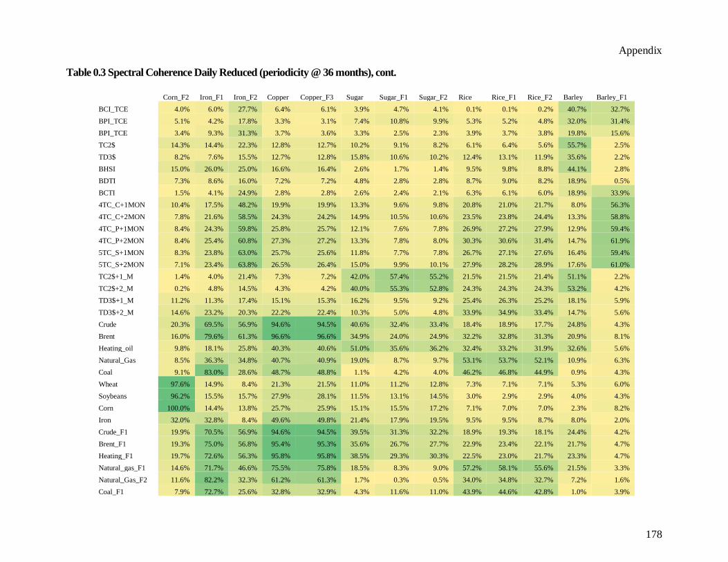
Appendix
178
Table 0.3 Spectral Coherence Daily Reduced (periodicity @ 36 months), cont.
Corn_F2 Iron_F1 Iron_F2 Copper Copper_F3 Sugar Sugar_F1 Sugar_F2 Rice Rice_F1 Rice_F2 Barley Barley_F1
BCI_TCE 4.0% 6.0% 27.7% 6.4% 6.1% 3.9% 4.7% 4.1% 0.1% 0.1% 0.2% 40.7% 32.7%
BPI_TCE 5.1% 4.2% 17.8% 3.3% 3.1% 7.4% 10.8% 9.9% 5.3% 5.2% 4.8% 32.0% 31.4%
BPI_TCE 3.4% 9.3% 31.3% 3.7% 3.6% 3.3% 2.5% 2.3% 3.9% 3.7% 3.8% 19.8% 15.6%
TC2$ 14.3% 14.4% 22.3% 12.8% 12.7% 10.2% 9.1% 8.2% 6.1% 6.4% 5.6% 55.7% 2.5%
TD3$ 8.2% 7.6% 15.5% 12.7% 12.8% 15.8% 10.6% 10.2% 12.4% 13.1% 11.9% 35.6% 2.2%
BHSI 15.0% 26.0% 25.0% 16.6% 16.4% 2.6% 1.7% 1.4% 9.5% 9.8% 8.8% 44.1% 2.8%
BDTI 7.3% 8.6% 16.0% 7.2% 7.2% 4.8% 2.8% 2.8% 8.7% 9.0% 8.2% 18.9% 0.5%
BCTI 1.5% 4.1% 24.9% 2.8% 2.8% 2.6% 2.4% 2.1% 6.3% 6.1% 6.0% 18.9% 33.9%
4TC_C+1MON 10.4% 17.5% 48.2% 19.9% 19.9% 13.3% 9.6% 9.8% 20.8% 21.0% 21.7% 8.0% 56.3%
4TC_C+2MON 7.8% 21.6% 58.5% 24.3% 24.2% 14.9% 10.5% 10.6% 23.5% 23.8% 24.4% 13.3% 58.8%
4TC_P+1MON 8.4% 24.3% 59.8% 25.8% 25.7% 12.1% 7.6% 7.8% 26.9% 27.2% 27.9% 12.9% 59.4%
4TC_P+2MON 8.4% 25.4% 60.8% 27.3% 27.2% 13.3% 7.8% 8.0% 30.3% 30.6% 31.4% 14.7% 61.9%
5TC_S+1MON 8.3% 23.8% 63.0% 25.7% 25.6% 11.8% 7.7% 7.8% 26.7% 27.1% 27.6% 16.4% 59.4%
5TC_S+2MON 7.1% 23.4% 63.8% 26.5% 26.4% 15.0% 9.9% 10.1% 27.9% 28.2% 28.9% 17.6% 61.0%
TC2$+1_M 1.4% 4.0% 21.4% 7.3% 7.2% 42.0% 57.4% 55.2% 21.5% 21.5% 21.4% 51.1% 2.2%
TC2$+2_M 0.2% 4.8% 14.5% 4.3% 4.2% 40.0% 55.3% 52.8% 24.3% 24.3% 24.3% 53.2% 4.2%
TD3$+1_M 11.2% 11.3% 17.4% 15.1% 15.3% 16.2% 9.5% 9.2% 25.4% 26.3% 25.2% 18.1% 5.9%
TD3$+2_M 14.6% 23.2% 20.3% 22.2% 22.4% 10.3% 5.0% 4.8% 33.9% 34.9% 33.4% 14.7% 5.6%
Crude 20.3% 69.5% 56.9% 94.6% 94.5% 40.6% 32.4% 33.4% 18.4% 18.9% 17.7% 24.8% 4.3%
Brent 16.0% 79.6% 61.3% 96.6% 96.6% 34.9% 24.0% 24.9% 32.2% 32.8% 31.3% 20.9% 8.1%
Heating_oil 9.8% 18.1% 25.8% 40.3% 40.6% 51.0% 35.6% 36.2% 32.4% 33.2% 31.9% 32.6% 5.6%
Natural_Gas 8.5% 36.3% 34.8% 40.7% 40.9% 19.0% 8.7% 9.7% 53.1% 53.7% 52.1% 10.9% 6.3%
Coal 9.1% 83.0% 28.6% 48.7% 48.8% 1.1% 4.2% 4.0% 46.2% 46.8% 44.9% 0.9% 4.3%
Wheat 97.6% 14.9% 8.4% 21.3% 21.5% 11.0% 11.2% 12.8% 7.3% 7.1% 7.1% 5.3% 6.0%
Soybeans 96.2% 15.5% 15.7% 27.9% 28.1% 11.5% 13.1% 14.5% 3.0% 2.9% 2.9% 4.0% 4.3%
Corn 100.0% 14.4% 13.8% 25.7% 25.9% 15.1% 15.5% 17.2% 7.1% 7.0% 7.0% 2.3% 8.2%
Iron 32.0% 32.8% 8.4% 49.6% 49.8% 21.4% 17.9% 19.5% 9.5% 9.5% 8.7% 8.0% 2.0%
Crude_F1 19.9% 70.5% 56.9% 94.6% 94.5% 39.5% 31.3% 32.2% 18.9% 19.3% 18.1% 24.4% 4.2%
Brent_F1 19.3% 75.0% 56.8% 95.4% 95.3% 35.6% 26.7% 27.7% 22.9% 23.4% 22.1% 21.7% 4.7%
Heating_F1 19.7% 72.6% 56.3% 95.8% 95.8% 38.5% 29.3% 30.3% 22.5% 23.0% 21.7% 23.3% 4.7%
Natural_gas_F1 14.6% 71.7% 46.6% 75.5% 75.8% 18.5% 8.3% 9.0% 57.2% 58.1% 55.6% 21.5% 3.3%
Natural_Gas_F2 11.6% 82.2% 32.3% 61.2% 61.3% 1.7% 0.3% 0.5% 34.0% 34.8% 32.7% 7.2% 1.6%
Coal_F1 7.9% 72.7% 25.6% 32.8% 32.9% 4.3% 11.6% 11.0% 43.9% 44.6% 42.8% 1.0% 3.9%

Appendix
179
Coal_F2 8.6% 83.6% 30.5% 46.1% 46.2% 1.3% 5.1% 4.9% 43.6% 44.3% 42.4% 1.4% 3.4%
Wheat_F1 98.0% 17.8% 13.1% 27.3% 27.6% 13.5% 12.2% 13.9% 13.4% 13.1% 13.2% 3.5% 9.8%
Wheat_F2 97.4% 19.3% 14.2% 28.5% 28.8% 12.1% 10.6% 12.2% 14.9% 14.6% 14.7% 3.7% 10.3%
Soybeans_F1 95.9% 14.1% 16.2% 28.2% 28.4% 14.5% 16.8% 18.3% 2.1% 2.1% 2.0% 3.1% 4.8%
Soybeans_F2 96.6% 15.8% 17.2% 30.1% 30.2% 14.5% 16.3% 17.8% 3.1% 3.1% 3.0% 3.5% 4.9%
Corn_F1 99.7% 13.4% 13.4% 25.4% 25.5% 16.6% 17.8% 19.5% 5.2% 5.0% 5.1% 2.6% 6.8%
Corn_F2 100.0% 14.8% 14.1% 26.3% 26.5% 15.3% 15.7% 17.4% 7.1% 7.0% 7.0% 2.5% 8.0%
Iron_F1 14.8% 100.0% 63.6% 74.4% 74.4% 6.3% 2.2% 2.7% 42.6% 43.1% 41.6% 6.0% 11.9%
Iron_F2 14.1% 63.6% 100.0% 67.3% 66.9% 25.9% 20.3% 20.3% 25.5% 26.0% 25.5% 23.3% 31.0%
Copper 26.3% 74.4% 67.3% 100.0% 100.0% 42.4% 31.0% 32.2% 34.0% 34.5% 33.2% 22.5% 11.4%
Copper_F3 26.5% 74.4% 66.9% 100.0% 100.0% 42.4% 31.0% 32.2% 34.4% 34.9% 33.6% 22.2% 11.4%
Sugar 15.3% 6.3% 25.9% 42.4% 42.4% 100.0% 95.8% 96.3% 3.4% 3.5% 3.4% 39.5% 5.4%
Sugar_F1 15.7% 2.2% 20.3% 31.0% 31.0% 95.8% 100.0% 99.9% 0.0% 0.0% 0.0% 42.3% 2.0%
Sugar_F2 17.4% 2.7% 20.3% 32.2% 32.2% 96.3% 99.9% 100.0% 0.0% 0.0% 0.0% 40.5% 2.2%
Rice 7.1% 42.6% 25.5% 34.0% 34.4% 3.4% 0.0% 0.0% 100.0% 100.0% 100.0% 1.2% 25.8%
Rice_F1 7.0% 43.1% 26.0% 34.5% 34.9% 3.5% 0.0% 0.0% 100.0% 100.0% 99.9% 1.1% 25.9%
Rice_F2 7.0% 41.6% 25.5% 33.2% 33.6% 3.4% 0.0% 0.0% 100.0% 99.9% 100.0% 1.5% 27.5%
Barley 2.5% 6.0% 23.3% 22.5% 22.2% 39.5% 42.3% 40.5% 1.2% 1.1% 1.5% 100.0% 14.1%
Barley_F1 8.0% 11.9% 31.0% 11.4% 11.4% 5.4% 2.0% 2.2% 25.8% 25.9% 27.5% 14.1% 100.0%
Barley_F2 0.4% 33.5% 50.9% 38.6% 38.4% 20.7% 9.9% 10.0% 49.1% 49.8% 49.9% 26.6% 52.6%
Canola 79.6% 4.5% 2.2% 6.8% 6.8% 6.5% 11.6% 12.4% 5.4% 5.7% 5.4% 6.8% 0.0%
Canola_F1 85.0% 5.2% 3.3% 9.2% 9.2% 6.4% 10.7% 11.6% 2.9% 3.1% 2.8% 6.6% 0.2%
Canola_F2 87.1% 5.8% 5.1% 11.3% 11.4% 7.3% 11.5% 12.5% 2.1% 2.3% 2.1% 5.9% 0.5%
BDI 4.8% 5.1% 23.8% 5.6% 5.4% 3.9% 4.9% 4.3% 0.5% 0.4% 0.5% 38.8% 31.4%
BLPG1 1.4% 12.6% 4.5% 0.5% 0.5% 29.2% 40.7% 38.8% 17.2% 17.1% 16.4% 38.1% 9.1%
TD3 7.1% 6.6% 14.4% 11.5% 11.6% 16.4% 10.8% 10.6% 12.5% 13.1% 12.0% 30.2% 1.5%
TC2_37 14.4% 17.7% 24.3% 13.9% 13.8% 7.2% 6.4% 5.6% 6.4% 6.6% 5.9% 53.9% 2.6%

Appendix
180
Table 0.3 Spectral Coherence Daily Reduced (periodicity @ 36 months), cont.
Barley_F2 Canola Canola_F1 Canola_F2 BDI BLPG1 TD3 TC2_37
BCI_TCE 33.7% 5.4% 5.7% 4.2% 98.8% 36.9% 32.9% 37.7%
BPI_TCE 16.2% 2.6% 3.0% 2.5% 87.7% 48.2% 32.7% 25.2%
BPI_TCE 11.8% 3.4% 3.5% 3.1% 39.9% 17.2% 8.0% 12.4%
TC2$ 19.4% 18.4% 19.5% 17.9% 31.4% 23.8% 31.1% 99.2%
TD3$ 25.1% 13.8% 14.0% 12.8% 33.6% 16.1% 98.7% 33.8%
BHSI 20.8% 20.7% 21.0% 18.8% 34.7% 13.9% 25.4% 96.8%
BDTI 11.0% 7.7% 7.9% 6.8% 59.8% 18.0% 75.9% 42.4%
BCTI 16.1% 0.7% 0.8% 0.5% 49.3% 36.0% 9.1% 7.8%
4TC_C+1MON 42.0% 1.7% 2.0% 2.8% 23.8% 3.4% 2.5% 3.3%
4TC_C+2MON 51.4% 0.3% 0.6% 1.2% 24.6% 6.0% 3.7% 7.5%
4TC_P+1MON 52.9% 0.3% 0.6% 1.3% 22.9% 4.1% 4.1% 7.2%
4TC_P+2MON 55.9% 0.1% 0.4% 1.0% 23.9% 4.1% 4.7% 7.4%
5TC_S+1MON 55.6% 0.3% 0.6% 1.3% 23.9% 6.7% 7.3% 9.9%
5TC_S+2MON 59.8% 0.1% 0.2% 0.6% 26.1% 7.4% 8.0% 10.8%
TC2$+1_M 1.6% 6.0% 4.1% 4.3% 20.3% 66.6% 12.9% 32.9%
TC2$+2_M 0.7% 2.3% 1.1% 1.1% 20.7% 69.4% 13.8% 34.3%
TD3$+1_M 25.4% 15.3% 15.8% 15.4% 7.4% 8.7% 80.6% 24.8%
TD3$+2_M 23.6% 16.8% 17.5% 17.2% 8.6% 12.2% 73.7% 28.0%
Crude 25.6% 6.3% 8.3% 10.2% 6.8% 0.5% 7.9% 11.4%
Brent 38.0% 3.7% 4.8% 5.9% 6.1% 1.9% 11.6% 14.5%
Heating_oil 40.5% 8.9% 8.5% 8.1% 6.4% 3.2% 74.0% 21.6%
Natural_Gas 38.7% 1.7% 1.4% 1.0% 19.8% 7.6% 43.9% 17.2%
Coal 20.1% 6.6% 6.0% 5.5% 4.1% 43.1% 7.0% 13.9%
Wheat 1.8% 79.0% 84.5% 85.6% 9.7% 2.9% 10.8% 24.2%
Soybeans 1.0% 84.8% 89.9% 92.2% 3.3% 1.0% 7.6% 14.5%
Corn 0.3% 79.2% 84.7% 86.8% 4.7% 1.5% 6.8% 14.0%
Iron 1.5% 17.4% 21.3% 22.4% 11.7% 11.9% 2.8% 9.8%
Crude_F1 25.6% 6.1% 8.1% 9.9% 6.8% 0.6% 7.9% 11.6%
Brent_F1 27.3% 5.3% 7.2% 8.9% 6.1% 1.6% 8.3% 12.2%
Heating_F1 28.1% 5.6% 7.5% 9.2% 6.1% 1.1% 9.2% 12.1%
Natural_gas_F1 43.0% 7.6% 7.7% 7.3% 11.1% 11.7% 35.5% 31.9%
Natural_Gas_F2 19.1% 6.6% 7.0% 6.8% 8.6% 31.7% 14.0% 17.7%
Coal_F1 19.1% 9.2% 8.1% 7.1% 5.6% 45.5% 7.8% 17.3%

Appendix
181
Coal_F2 21.8% 8.7% 7.6% 6.7% 5.2% 39.0% 6.6% 16.7%
Wheat_F1 0.5% 70.2% 76.5% 78.5% 8.1% 2.9% 8.7% 18.5%
Wheat_F2 0.6% 68.4% 75.1% 77.2% 7.6% 3.4% 8.6% 18.9%
Soybeans_F1 0.7% 85.6% 90.2% 92.6% 2.2% 0.9% 6.2% 12.2%
Soybeans_F2 0.5% 84.0% 89.0% 91.5% 2.4% 0.8% 6.4% 12.5%
Corn_F1 0.6% 82.6% 87.4% 89.4% 4.3% 1.3% 6.8% 13.7%
Corn_F2 0.4% 79.6% 85.0% 87.1% 4.8% 1.4% 7.1% 14.4%
Iron_F1 33.5% 4.5% 5.2% 5.8% 5.1% 12.6% 6.6% 17.7%
Iron_F2 50.9% 2.2% 3.3% 5.1% 23.8% 4.5% 14.4% 24.3%
Copper 38.6% 6.8% 9.2% 11.3% 5.6% 0.5% 11.5% 13.9%
Copper_F3 38.4% 6.8% 9.2% 11.4% 5.4% 0.5% 11.6% 13.8%
Sugar 20.7% 6.5% 6.4% 7.3% 3.9% 29.2% 16.4% 7.2%
Sugar_F1 9.9% 11.6% 10.7% 11.5% 4.9% 40.7% 10.8% 6.4%
Sugar_F2 10.0% 12.4% 11.6% 12.5% 4.3% 38.8% 10.6% 5.6%
Rice 49.1% 5.4% 2.9% 2.1% 0.5% 17.2% 12.5% 6.4%
Rice_F1 49.8% 5.7% 3.1% 2.3% 0.4% 17.1% 13.1% 6.6%
Rice_F2 49.9% 5.4% 2.8% 2.1% 0.5% 16.4% 12.0% 5.9%
Barley 26.6% 6.8% 6.6% 5.9% 38.8% 38.1% 30.2% 53.9%
Barley_F1 52.6% 0.0% 0.2% 0.5% 31.4% 9.1% 1.5% 2.6%
Barley_F2 100.0% 15.9% 12.8% 9.9% 29.4% 4.0% 23.0% 19.4%
Canola 15.9% 100.0% 99.3% 98.5% 5.3% 1.1% 12.1% 18.2%
Canola_F1 12.8% 99.3% 100.0% 99.7% 5.7% 0.5% 12.1% 19.2%
Canola_F2 9.9% 98.5% 99.7% 100.0% 4.2% 0.5% 11.0% 17.5%
BDI 29.4% 5.3% 5.7% 4.2% 100.0% 36.8% 35.1% 34.7%
BLPG1 4.0% 1.1% 0.5% 0.5% 36.8% 100.0% 13.5% 21.8%
TD3 23.0% 12.1% 12.1% 11.0% 35.1% 13.5% 100.0% 29.3%
TC2_37 19.4% 18.2% 19.2% 17.5% 34.7% 21.8% 29.3% 100.0%

Appendix
182
Table 0.4 Reference Variable: Baltic Dry Index (BDI)
Monthly Dataset Weekly Dataset Daily Dataset
# Variable No. of Factors - 4 Cycl. No. of Factors - 4 Cycl. No. of Factors - 4 Cycl.
1 BCI_TCE 0.8 0.0 0.5 0.0 0.6 0.0
2 BPI_TCE 0.0 0.0 0.8 0.0 -1.5 0.0
3 BSI_TCE -1.0 0.0 -1.8 0.0 -11.1 0.0
4 TC2$ -8.0 3.1 -15.4 3.1 -4.5 3.1
5 TD3$ -16.0 3.1 -4.4 3.1 -3.6 0.0
6 BHSI -5.2 3.1 -12.8 3.1 -4.7 3.1
7 BDTI -13.5 3.1 3.6 0.0 0.2 0.0
8 BCTI -2.3 0.0 -2.2 0.0 -14.2 0.0
9 4TC_C+1MON 0.6 0.0 2.8 0.0 7.9 0.0
10 4TC_C+2MON 0.8 0.0 3.2 0.0 9.6 0.0
11 4TC_P+1MON 1.2 0.0 4.6 0.0 9.4 0.0
12 4TC_P+2MON 1.5 0.0 5.2 0.0 9.4 0.0
13 5TC_S+1MON 0.9 0.0 5.8 0.0 11.1 0.0
14 5TC_S+2MON 1.6 0.0 5.5 0.0 10.4 0.0
15 TC2$+1_M -10.0 3.1 -12.7 3.1 -2.0 3.1
16 TC2$+2_M -11.9 3.1 -12.1 3.1 -2.4 3.1
17 TD3$+1_M -16.0 3.1 -6.2 3.1 -3.7 0.0
18 TD3$+2_M -16.0 3.1 -5.3 3.1 -3.4 0.0
19 Crude 16.6 0.0 -1.4 0.0 -12.9 0.0
20 Brent 16.3 0.0 -0.5 0.0 -13.4 0.0
21 Heating_oil 16.3 0.0 -7.8 0.0 -5.1 0.0
22 Natural_Gas -2.9 0.0 -4.2 0.0 -2.7 0.0
23 Coal 9.9 0.0 2.4 0.0 -6.9 0.0
24 Wheat -0.7 3.1 -11.8 3.1 -3.7 3.1
25 Soybeans -4.0 0.0 11.7 3.1 -2.9 3.1
26 Corn 3.7 3.1 17.9 3.1 -4.7 3.1
27 Iron 2.1 0.0 9.8 0.0 -2.1 0.0
28 CME_Crude_F1 16.8 0.0 -1.6 0.0 -12.9 0.0
29 ICE_Brent_F1 16.4 0.0 -0.6 0.0 -12.6 0.0
30 CME_Heating_F1 16.9 0.0 -0.6 0.0 -12.5 0.0
31 CME_Natural_gas_F1 -2.7 0.0 -3.0 0.0 -7.4 0.0
32 ICE_Natural_Gas_F2 6.3 0.0 -0.2 0.0 -6.9 0.0
33 ICE_Coal_F1 12.6 0.0 7.0 0.0 -7.7 0.0
34 ICE_Coal_F2 10.6 0.0 6.1 0.0 -8.7 0.0
35 CME_Wheat_F1 0.5 3.1 -9.9 3.1 -4.0 3.1
36 CME_Wheat_F2 0.4 3.1 -9.5 3.1 -3.9 3.1
37 CME_Soybeans_F1 4.1 3.1 10.8 3.1 -4.1 3.1
38 CME_Soybeans_F2 3.9 3.1 11.3 3.1 -3.4 3.1
39 CME_Corn_F1 2.6 3.1 -17.1 3.1 -4.4 3.1
40 CME_Corn_F2 2.3 3.1 -17.3 3.1 -4.4 3.1
41 CME_Iron_F1 11.1 0.0 11.4 0.0 -13.9 0.0
42 CME_Iron_F2 13.0 0.0 -6.6 0.0 17.0 0.0
43 Copper 14.7 0.0 -4.6 0.0 -14.0 0.0
44 Copper_F3 14.7 0.0 -4.5 0.0 -14.0 0.0
45 Sugar -15.7 0.0 -3.8 0.0 -17.2 0.0
46 Sugar_F1 -15.8 0.0 -3.8 0.0 -16.9 0.0
47 Sugar_F2 -14.7 0.0 -3.9 0.0 -17.0 0.0
48 Rice 6.1 3.1 -3.7 3.1 5.3 0.0
49 Rice_F1 7.1 3.1 -4.2 3.1 5.1 0.0
50 Rice_F2 6.3 3.1 -4.5 3.1 6.5 0.0
51 Barley 4.9 3.1 12.5 3.1 11.6 3.1
52 Barley_F1 -0.3 0.0 16.0 0.0 16.2 0.0
53 Barley_F2 0.3 0.0 -12.9 0.0 -16.1 0.0
54 Canola -3.8 3.1 13.9 3.1 -2.3 3.1
55 Canola_F1 -0.9 3.1 12.2 3.1 -2.4 3.1
56 Canola_F2 -0.9 3.1 13.9 3.1 -2.5 3.1
57 BDI 0.0 0.0 0.0 0.0 0.0 0.0
58 BLPG1 -16.2 3.1 -11.7 3.1 -0.9 3.1
59 TD3 -16.0 3.1 -4.1 3.1 -2.9 0.0
60 TC2_37 -7.9 3.1 -14.7 3.1 -4.5 3.1
61 Urea 14.4 0.0 -14.3 3.1 - -
62 DAP 1.4 3.1 -3.7 3.1 - -
63 Ammonia -15.0 3.1 -10.5 3.1 - -
64 Scrap VLCC 6.9 0.0 - - - - 65 Scrap Cape/Pana 4.3 0.0 - - - -

Appendix
183
Note: The details of the parameters are denoted in Table 3.1
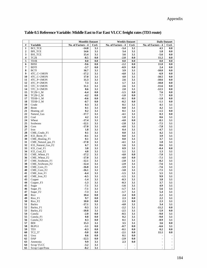
Appendix
184
Table 0.5 Reference Variable: Middle East to Far East VLCC freight rates (TD3 route)
Monthly Dataset Weekly Dataset Daily Dataset
# Variable No. of Factors - 4 Cycl. No. of Factors - 4 Cycl. No. of Factors - 4 Cycl.
1 BCI_TCE -14.8 3.1 -3.4 3.1 4.5 0.0
2 BPI_TCE 14.6 3.1 3.4 3.1 1.8 0.0
3 BSI_TCE 15.4 3.1 3.6 3.1 -5.6 0.0
4 TC2$ -8.5 0.0 -2.0 0.0 11.2 0.0
5 TD3$ 0.0 0.0 0.0 0.0 0.0 0.0
6 BHSI -9.6 0.0 -2.2 0.0 11.0 0.0
7 BDTI -3.7 0.0 -0.9 0.0 2.4 0.0
8 BCTI 16.7 3.1 3.9 3.1 -10.0 0.0
9 4TC_C+1MON -17.2 3.1 -4.0 3.1 -6.9 0.0
10 4TC_C+2MON 17.0 3.1 4.0 3.1 -10.5 0.0
11 4TC_P+1MON 11.3 3.1 2.6 3.1 -10.6 0.0
12 4TC_P+2MON 7.3 3.1 1.7 3.1 -10.8 0.0
13 5TC_S+1MON 11.1 3.1 2.6 3.1 -11.6 0.0
14 5TC_S+2MON 8.6 3.1 2.0 3.1 -12.5 0.0
15 TC2$+1_M -6.4 0.0 -1.5 0.0 7.6 0.0
16 TC2$+2_M -4.2 0.0 -1.0 0.0 7.7 0.0
17 TD3$+1_M -0.6 0.0 -0.1 0.0 -1.0 0.0
18 TD3$+2_M -0.7 0.0 -0.2 0.0 -1.1 0.0
19 Crude 0.3 3.1 0.1 3.1 4.1 3.1
20 Brent 0.1 3.1 0.0 3.1 4.2 3.1
21 Heating_oil 0.2 3.1 0.1 3.1 -1.5 0.0
22 Natural_Gas -17.7 3.1 -4.1 3.1 0.3 0.0
23 Coal 4.2 3.1 1.0 3.1 0.6 3.1
24 Wheat -17.4 3.1 -4.0 0.0 -8.1 3.1
25 Soybeans -12.1 3.1 -2.8 3.1 -7.5 3.1
26 Corn -17.0 3.1 -4.0 3.1 -7.8 3.1
27 Iron 1.8 3.1 0.4 3.1 -4.7 3.1
28 CME_Crude_F1 0.1 3.1 0.0 3.1 4.2 3.1
29 ICE_Brent_F1 -0.1 3.1 0.0 3.1 3.9 3.1
30 CME_Heating_F1 0.1 3.1 0.0 3.1 3.7 3.1
31 CME_Natural_gas_F1 -17.8 3.1 -4.1 3.1 1.8 3.1
32 ICE_Natural_Gas_F2 6.7 3.1 1.6 3.1 0.6 3.1
33 ICE_Coal_F1 3.8 3.1 0.9 3.1 -0.4 0.0
34 ICE_Coal_F2 4.8 3.1 1.1 3.1 1.3 3.1
35 CME_Wheat_F1 -17.2 3.1 -4.0 0.0 -7.0 3.1
36 CME_Wheat_F2 -17.0 3.1 -4.0 0.0 -7.1 3.1
37 CME_Soybeans_F1 -12.1 3.1 -2.8 3.1 -8.2 3.1
38 CME_Soybeans_F2 -12.4 3.1 -2.9 3.1 -7.6 3.1
39 CME_Corn_F1 -16.8 3.1 -3.9 3.1 -7.6 3.1
40 CME_Corn_F2 -16.1 3.1 -3.8 3.1 -7.5 3.1
41 CME_Iron_F1 -6.4 3.1 -1.5 3.1 5.5 3.1
42 CME_Iron_F2 -6.5 3.1 -1.5 3.1 9.9 3.1
43 Copper -1.4 3.1 -0.3 3.1 3.8 3.1
44 Copper_F3 -1.3 3.1 -0.3 3.1 3.7 3.1
45 Sugar -7.1 3.1 -1.6 3.1 4.9 3.1
46 Sugar_F1 -7.1 3.1 -1.7 3.1 5.6 3.1
47 Sugar_F2 -7.3 3.1 -1.7 3.1 5.4 3.1
48 Rice 10.4 0.0 2.4 0.0 2.2 3.1
49 Rice_F1 9.7 0.0 2.3 0.0 2.2 3.1
50 Rice_F2 10.0 0.0 2.3 0.0 2.3 3.1
51 Barley -17.1 3.1 -4.0 3.1 3.4 3.1
52 Barley_F1 -9.3 3.1 -2.2 3.1 -11.2 0.0
53 Barley_F2 -10.8 3.1 -2.5 3.1 -5.9 0.0
54 Canola -2.0 0.0 -0.5 3.1 -9.0 3.1
55 Canola_F1 0.8 0.0 0.2 3.1 -9.0 3.1
56 Canola_F2 0.3 0.0 0.1 3.1 -8.9 3.1
57 BDI 15.3 3.1 3.5 3.1 3.6 0.0
58 BLPG1 -3.1 0.0 -0.7 0.0 -6.6 3.1
59 TD3 -0.3 0.0 -0.1 0.0 0.2 0.0
60 TC2_37 -9.0 0.0 -2.1 0.0 11.1 0.0
61 Urea 0.6 0.0 0.1 0.0 - -
62 DAP -12.5 0.0 -2.9 0.0 - -
63 Ammonia 9.9 3.1 2.3 0.0 - -
64 Scrap VLCC -3.2 3.1 - - - - 65 Scrap Cape/Pana -8.2 3.1 - - - -

Appendix
185
Note: The details of the parameters are denoted in Table 3.1

Appendix
186
Table 0.6 Reference Variable: North West Europe to US Atlantic Coast (TC2 route)
Monthly Dataset Weekly Dataset Daily Dataset
# Variable No. of Factors - 4 Cycl. No. of Factors - 4 Cycl. No. of Factors - 4 Cycl.
1 BCI_TCE -17.9 0.0 -4.2 3.1 3.6 3.1
2 BPI_TCE 5.1 3.1 1.2 3.1 8.0 3.1
3 BSI_TCE 6.0 3.1 1.4 3.1 14.8 3.1
4 TC2$ 0.2 0.0 0.1 0.0 -0.1 0.0
5 TD3$ 9.0 0.0 2.1 0.0 -11.1 0.0
6 BHSI -0.2 0.0 -0.1 0.0 0.2 0.0
7 BDTI 4.8 0.0 1.1 0.0 -4.5 0.0
8 BCTI 6.9 3.1 1.6 3.1 -17.3 3.1
9 4TC_C+1MON 14.5 3.1 3.4 3.1 -8.6 3.1
10 4TC_C+2MON 11.6 3.1 2.7 3.1 -10.2 3.1
11 4TC_P+1MON 0.8 3.1 0.2 3.1 -10.9 3.1
12 4TC_P+2MON -4.9 3.1 -1.1 3.1 -11.0 3.1
13 5TC_S+1MON 3.0 3.1 0.7 3.1 -11.3 3.1
14 5TC_S+2MON -0.3 3.1 -0.1 3.1 -10.5 3.1
15 TC2$+1_M 1.8 0.0 0.4 0.0 -2.2 0.0
16 TC2$+2_M 3.3 0.0 0.8 0.0 -2.3 0.0
17 TD3$+1_M 8.0 0.0 1.9 0.0 -13.0 0.0
18 TD3$+2_M 8.2 0.0 1.9 0.0 -13.2 0.0
19 Crude -8.2 3.1 -1.9 3.1 15.2 3.1
20 Brent -7.4 3.1 -1.7 3.1 15.5 3.1
21 Heating_oil -7.1 3.1 -1.6 3.1 13.4 3.1
22 Natural_Gas 8.8 3.1 2.1 3.1 8.7 3.1
23 Coal -3.0 3.1 -0.7 0.0 -12.0 0.0
24 Wheat -5.6 0.0 -1.3 3.1 2.7 3.1
25 Soybeans 8.4 3.1 1.9 3.1 4.1 3.1
26 Corn -4.5 0.0 -1.0 3.1 3.3 3.1
27 Iron -5.3 3.1 -1.2 3.1 5.8 3.1
28 CME_Crude_F1 -8.3 3.1 -1.9 3.1 15.2 3.1
29 ICE_Brent_F1 -7.8 3.1 -1.8 3.1 15.0 3.1
30 CME_Heating_F1 -7.3 3.1 -1.7 3.1 14.9 3.1
31 CME_Natural_gas_F1 8.4 3.1 1.9 3.1 13.6 3.1
32 ICE_Natural_Gas_F2 0.5 0.0 0.1 0.0 -11.9 0.0
33 ICE_Coal_F1 -0.7 3.1 -0.2 0.0 -12.3 0.0
34 ICE_Coal_F2 -1.3 3.1 -0.3 0.0 -13.1 0.0
35 CME_Wheat_F1 -5.8 0.0 -1.3 3.1 3.3 3.1
36 CME_Wheat_F2 -5.8 0.0 -1.4 3.1 3.4 3.1
37 CME_Soybeans_F1 8.3 3.1 1.9 3.1 3.7 3.1
38 CME_Soybeans_F2 7.9 3.1 1.8 3.1 4.1 3.1
39 CME_Corn_F1 -5.4 0.0 -1.2 3.1 3.4 3.1
40 CME_Corn_F2 -5.4 0.0 -1.3 3.1 3.4 3.1
41 CME_Iron_F1 -14.6 3.1 -3.4 3.1 15.8 3.1
42 CME_Iron_F2 -14.9 3.1 -3.5 3.1 -16.2 3.1
43 Copper -9.1 3.1 -2.1 3.1 15.1 3.1
44 Copper_F3 -9.0 3.1 -2.1 3.1 15.1 3.1
45 Sugar -17.0 3.1 -3.9 3.1 -17.2 3.1
46 Sugar_F1 -17.0 3.1 -4.0 3.1 -16.4 3.1
47 Sugar_F2 -17.1 3.1 -4.0 3.1 -16.5 3.1
48 Rice 8.2 3.1 1.9 3.1 12.8 3.1
49 Rice_F1 9.2 3.1 2.1 3.1 12.8 3.1
50 Rice_F2 8.5 3.1 2.0 3.1 12.8 3.1
51 Barley 5.4 3.1 1.3 3.1 16.4 3.1
52 Barley_F1 -17.2 3.1 -4.0 0.0 -4.7 3.1
53 Barley_F2 17.8 3.1 4.1 0.0 17.9 3.1
54 Canola -1.1 0.0 -0.3 3.1 -2.7 0.0
55 Canola_F1 3.3 3.1 0.8 3.1 -2.8 0.0
56 Canola_F2 -2.6 0.0 -0.6 3.1 3.0 3.1
57 BDI 5.9 3.1 1.4 3.1 4.5 3.1
58 BLPG1 2.6 0.0 0.6 0.0 -4.3 0.0
59 TD3 8.6 0.0 2.0 0.0 -10.2 0.0
60 TC2_37 0.0 0.0 0.0 0.0 0.0 0.0
61 Urea 9.7 0.0 2.3 0.0 - -
62 DAP -1.6 0.0 -0.4 3.1 - -
63 Ammonia 0.4 0.0 0.1 0.0 - -
64 Scrap VLCC -12.2 3.1 - - - - 65 Scrap Cape/Pana -14.8 3.1 - - - -

Appendix
187
Note: The details of the parameters are denoted in Table 3.1

Appendix
188
Table 0.7 Reference Variable: Panamax T/C Futures second-near month
Monthly Dataset Weekly Dataset Daily Dataset
# Variable No. of Factors - 4 Cycl. No. of Factors - 4 Cycl. No. of Factors - 4 Cycl.
1 BCI_TCE 0.7 0.0 -4.5 0.0 -9.0 0.0
2 BPI_TCE -2.0 0.0 -4.8 0.0 -11.3 0.0
3 BSI_TCE -4.7 0.0 -7.8 0.0 13.3 0.0
4 TC2$ 6.2 3.1 -2.3 3.1 11.7 3.1
5 TD3$ -6.1 3.1 9.8 3.1 10.8 0.0
6 BHSI 2.4 3.1 -0.3 3.1 9.9 3.1
7 BDTI 5.7 0.0 -5.0 0.0 13.3 3.1
8 BCTI -7.8 0.0 -9.6 0.0 12.4 0.0
9 4TC_C+1MON 0.4 0.0 -1.3 0.0 -0.2 0.0
10 4TC_C+2MON 0.2 0.0 -0.7 0.0 0.0 0.0
11 4TC_P+1MON -0.1 0.0 -0.4 0.0 -0.1 0.0
12 4TC_P+2MON 0.0 0.0 0.0 0.0 0.0 0.0
13 5TC_S+1MON -0.7 0.0 0.5 0.0 0.6 0.0
14 5TC_S+2MON -0.6 0.0 0.4 0.0 0.0 0.0
15 TC2$+1_M -4.0 3.1 -4.7 3.1 -17.8 3.1
16 TC2$+2_M -7.6 3.1 -4.2 3.1 -15.6 3.1
17 TD3$+1_M -11.9 3.1 1.6 3.1 5.9 0.0
18 TD3$+2_M -12.1 3.1 2.2 3.1 5.4 0.0
19 Crude 9.5 0.0 -4.3 0.0 6.8 0.0
20 Brent 9.1 0.0 -2.1 0.0 6.3 0.0
21 Heating_oil 8.9 0.0 -12.8 0.0 6.8 0.0
22 Natural_Gas -8.6 0.0 -11.3 0.0 13.7 0.0
23 Coal 4.3 0.0 4.5 0.0 8.3 0.0
24 Wheat -1.7 3.1 -7.0 3.1 -6.9 3.1
25 Soybeans 3.0 3.1 -14.0 3.1 -6.8 3.1
26 Corn 7.0 3.1 -10.7 3.1 -6.4 3.1
27 Iron 0.5 0.0 2.4 0.0 -16.2 0.0
28 CME_Crude_F1 9.9 0.0 -4.6 0.0 6.8 0.0
29 ICE_Brent_F1 9.3 0.0 -2.1 0.0 6.8 0.0
30 CME_Heating_F1 11.6 0.0 -2.5 0.0 6.9 0.0
31 CME_Natural_gas_F1 -8.9 0.0 -11.8 0.0 8.6 0.0
32 ICE_Natural_Gas_F2 -0.3 0.0 -8.0 0.0 9.2 0.0
33 ICE_Coal_F1 9.6 0.0 6.3 0.0 9.2 0.0
34 ICE_Coal_F2 5.2 0.0 5.7 0.0 8.6 0.0
35 CME_Wheat_F1 0.1 3.1 -6.1 3.1 -6.4 3.1
36 CME_Wheat_F2 -0.1 3.1 -6.5 3.1 -6.7 3.1
37 CME_Soybeans_F1 3.5 3.1 -13.5 3.1 -6.5 3.1
38 CME_Soybeans_F2 3.6 3.1 -12.9 3.1 -6.8 3.1
39 CME_Corn_F1 3.8 3.1 -10.7 3.1 -6.3 3.1
40 CME_Corn_F2 2.6 3.1 -10.5 3.1 -6.4 3.1
41 CME_Iron_F1 7.6 0.0 2.2 0.0 5.4 0.0
42 CME_Iron_F2 8.3 0.0 0.8 0.0 3.1 0.0
43 Copper 10.9 0.0 -10.0 0.0 6.5 0.0
44 Copper_F3 11.0 0.0 -9.5 0.0 6.5 0.0
45 Sugar 6.0 0.0 -8.9 0.0 4.1 0.0
46 Sugar_F1 6.5 0.0 -9.1 0.0 3.6 0.0
47 Sugar_F2 5.8 0.0 -8.7 0.0 3.6 0.0
48 Rice -6.7 0.0 0.5 0.0 6.5 0.0
49 Rice_F1 -7.8 0.0 -0.7 3.1 6.6 0.0
50 Rice_F2 -6.9 0.0 -0.8 3.1 6.5 0.0
51 Barley 7.9 3.1 -17.1 3.1 -12.6 3.1
52 Barley_F1 4.8 0.0 7.8 0.0 7.7 0.0
53 Barley_F2 5.8 0.0 -17.4 0.0 8.5 0.0
54 Canola -0.7 3.1 -16.7 3.1 -8.9 3.1
55 Canola_F1 0.0 3.1 -17.3 3.1 -8.1 3.1
56 Canola_F2 -0.2 3.1 -16.3 3.1 -8.3 3.1
57 BDI -1.5 0.0 -5.2 0.0 -9.4 0.0
58 BLPG1 12.4 3.1 -8.1 3.1 10.6 3.1
59 TD3 -7.5 3.1 8.9 3.1 10.9 0.0
60 TC2_37 8.1 3.1 -1.4 3.1 11.0 3.1
61 Urea 6.8 0.0 -6.0 3.1 - -
62 DAP 6.6 3.1 -10.0 0.0 - -
63 Ammonia -7.8 0.0 4.9 3.1 - -
64 Scrap VLCC 3.5 0.0 - - - - 65 Scrap Cape/Pana 3.2 0.0 - - - -

Appendix
189
Note: The details of the parameters are denoted in Table 3.1

Appendix
190
Table 0.8 Reference variable: Crude Oil
Monthly Dataset Weekly Dataset Daily Dataset
# Variable No. of Factors - 4 Cycl. No. of Factors - 4 Cycl. No. of Factors - 4 Cycl.
1 BCI_TCE 15.1 3.1 2.9 0.0 14.1 0.0
2 BPI_TCE -16.4 0.0 -0.7 0.0 10.7 0.0
3 BSI_TCE -17.6 0.0 -0.6 0.0 6.3 0.0
4 TC2$ 8.1 3.1 -10.3 0.0 -15.2 3.1
5 TD3$ 0.4 3.1 -6.0 3.1 -4.1 3.1
6 BHSI 9.1 3.1 11.3 3.1 -15.4 3.1
7 BDTI -2.3 0.0 -3.8 3.1 -9.5 3.1
8 BCTI 17.5 0.0 -0.1 0.0 9.8 0.0
9 4TC_C+1MON -15.1 0.0 4.3 0.0 -7.4 0.0
10 4TC_C+2MON -13.3 0.0 3.8 0.0 -7.2 0.0
11 4TC_P+1MON -12.7 0.0 4.2 0.0 -7.5 0.0
12 4TC_P+2MON -9.5 0.0 4.3 0.0 -6.8 0.0
13 5TC_S+1MON -14.0 0.0 4.0 0.0 -7.1 0.0
14 5TC_S+2MON -10.9 0.0 2.9 0.0 -7.0 0.0
15 TC2$+1_M 5.9 3.1 -12.0 3.1 -15.6 3.1
16 TC2$+2_M 4.2 3.1 -7.3 3.1 -15.5 3.1
17 TD3$+1_M 0.5 3.1 -6.8 3.1 -1.0 3.1
18 TD3$+2_M -0.2 3.1 -6.5 3.1 -0.1 0.0
19 Crude 0.0 0.0 0.0 0.0 0.0 0.0
20 Brent -0.7 0.0 0.2 0.0 -0.1 0.0
21 Heating_oil -0.8 0.0 -5.8 0.0 2.2 0.0
22 Natural_Gas 16.1 0.0 -4.7 0.0 5.4 0.0
23 Coal -4.5 0.0 2.5 0.0 -0.5 0.0
24 Wheat 11.7 3.1 -5.2 3.1 -4.3 3.1
25 Soybeans -14.3 0.0 -2.8 0.0 2.2 0.0
26 Corn -12.9 0.0 -3.0 3.1 -3.2 3.1
27 Iron -6.9 0.0 2.2 0.0 2.1 0.0
28 CME_Crude_F1 0.1 0.0 0.0 0.0 0.0 0.0
29 ICE_Brent_F1 -0.5 0.0 0.3 0.0 0.0 0.0
30 CME_Heating_F1 -0.4 0.0 0.0 0.0 0.0 0.0
31 CME_Natural_gas_F1 16.8 0.0 -1.7 0.0 1.1 0.0
32 ICE_Natural_Gas_F2 -7.9 0.0 2.8 0.0 -0.1 0.0
33 ICE_Coal_F1 -4.5 0.0 3.7 0.0 -0.6 0.0
34 ICE_Coal_F2 -4.9 0.0 3.8 0.0 -0.7 0.0
35 CME_Wheat_F1 12.9 3.1 -6.3 3.1 -3.7 3.1
36 CME_Wheat_F2 12.8 3.1 -6.0 3.1 3.6 0.0
37 CME_Soybeans_F1 -14.7 0.0 -3.5 0.0 2.1 0.0
38 CME_Soybeans_F2 -14.8 0.0 -2.2 0.0 2.1 0.0
39 CME_Corn_F1 -13.4 0.0 4.4 0.0 3.1 0.0
40 CME_Corn_F2 -13.0 0.0 -4.1 3.1 3.2 0.0
41 CME_Iron_F1 2.4 0.0 -2.9 0.0 -1.2 0.0
42 CME_Iron_F2 2.8 0.0 -3.0 0.0 -2.5 0.0
43 Copper 0.3 0.0 -1.5 0.0 0.2 0.0
44 Copper_F3 0.2 0.0 -1.4 0.0 0.2 0.0
45 Sugar 4.7 0.0 -1.8 0.0 1.2 0.0
46 Sugar_F1 5.2 0.0 -1.6 0.0 1.2 0.0
47 Sugar_F2 4.8 0.0 -1.9 0.0 1.2 0.0
48 Rice -15.9 0.0 2.7 0.0 2.1 0.0
49 Rice_F1 -16.4 0.0 -3.1 3.1 2.1 0.0
50 Rice_F2 -16.1 0.0 -3.6 3.1 2.1 0.0
51 Barley -14.6 0.0 -5.7 0.0 -0.9 3.1
52 Barley_F1 4.5 0.0 -8.3 0.0 3.8 0.0
53 Barley_F2 3.1 0.0 -6.6 0.0 1.5 0.0
54 Canola 11.8 3.1 10.6 3.1 -4.2 3.1
55 Canola_F1 13.1 3.1 -9.5 0.0 3.8 0.0
56 Canola_F2 12.3 3.1 -6.3 0.0 3.4 0.0
57 BDI -16.6 0.0 1.4 0.0 12.9 0.0
58 BLPG1 5.9 3.1 -7.7 3.1 2.8 3.1
59 TD3 0.3 3.1 -6.0 3.1 -5.1 3.1
60 TC2_37 8.2 3.1 10.2 3.1 -15.2 3.1
61 Urea 0.3 0.0 15.9 3.1 - -
62 DAP 12.5 3.1 10.9 3.1 - -
63 Ammonia -5.8 0.0 16.7 3.1 - -
64 Scrap VLCC -2.4 0.0 - - - - 65 Scrap Cape/Pana -1.7 0.0 - - - -

Appendix
191
Note: The details of the parameters are denoted in Table 3.1

Appendix
192
Table 0.9 Reference Variable: Corn
Monthly Dataset Weekly Dataset Daily Dataset
# Variable No. of Factors - 4 Cycl. No. of Factors - 4 Cycl. No. of Factors - 4 Cycl.
1 BCI_TCE -8.7 3.1 -13.7 3.1 3.5 3.1
2 BPI_TCE -1.1 3.1 14.6 3.1 9.2 3.1
3 BSI_TCE 2.1 3.1 14.2 3.1 11.6 3.1
4 TC2$ 3.5 0.0 -5.2 0.0 -3.2 3.1
5 TD3$ 16.5 0.0 17.9 3.1 7.8 3.1
6 BHSI 3.9 0.0 1.8 3.1 -3.4 3.1
7 BDTI -14.1 3.1 12.8 3.1 3.0 3.1
8 BCTI 3.5 3.1 17.4 3.1 17.8 3.1
9 4TC_C+1MON -7.1 3.1 12.6 3.1 5.7 3.1
10 4TC_C+2MON -6.7 3.1 10.1 3.1 6.0 3.1
11 4TC_P+1MON -5.0 3.1 11.8 3.1 6.5 3.1
12 4TC_P+2MON -7.0 3.1 10.7 3.1 6.4 3.1
13 5TC_S+1MON -0.9 3.1 9.9 3.1 5.9 3.1
14 5TC_S+2MON -2.6 3.1 9.2 3.1 5.7 3.1
15 TC2$+1_M 5.5 0.0 -6.7 0.0 -14.8 3.1
16 TC2$+2_M 6.7 0.0 -7.9 0.0 -7.2 3.1
17 TD3$+1_M 16.5 0.0 11.7 3.1 8.3 3.1
18 TD3$+2_M 15.8 0.0 14.0 3.1 8.6 3.1
19 Crude 12.9 0.0 3.0 3.1 3.2 3.1
20 Brent 10.0 0.0 -4.0 0.0 4.1 3.1
21 Heating_oil 9.7 0.0 -12.9 0.0 4.8 3.1
22 Natural_Gas 2.5 0.0 9.9 0.0 0.1 3.1
23 Coal -8.3 3.1 -3.9 0.0 7.2 3.1
24 Wheat 1.2 0.0 0.8 0.0 0.2 0.0
25 Soybeans -0.7 0.0 -1.2 0.0 -0.4 0.0
26 Corn 0.0 0.0 0.0 0.0 0.0 0.0
27 Iron -0.9 3.1 6.1 3.1 0.4 3.1
28 CME_Crude_F1 13.0 0.0 2.8 3.1 3.3 3.1
29 ICE_Brent_F1 10.8 0.0 -3.5 0.0 3.5 3.1
30 CME_Heating_F1 11.2 0.0 -4.0 0.0 3.3 3.1
31 CME_Natural_gas_F1 2.9 0.0 -10.9 3.1 4.8 3.1
32 ICE_Natural_Gas_F2 -2.3 3.1 -6.5 3.1 6.7 3.1
33 ICE_Coal_F1 -2.4 3.1 -5.2 0.0 8.4 3.1
34 ICE_Coal_F2 -5.0 3.1 -4.4 0.0 8.3 3.1
35 CME_Wheat_F1 0.4 0.0 0.6 0.0 0.0 0.0
36 CME_Wheat_F2 0.4 0.0 0.7 0.0 0.0 0.0
37 CME_Soybeans_F1 -0.9 0.0 -1.3 0.0 -0.3 0.0
38 CME_Soybeans_F2 -1.0 0.0 -1.0 0.0 -0.3 0.0
39 CME_Corn_F1 -0.1 0.0 0.1 0.0 0.0 0.0
40 CME_Corn_F2 0.1 0.0 0.2 0.0 0.0 0.0
41 CME_Iron_F1 -10.3 3.1 -10.4 0.0 6.4 3.1
42 CME_Iron_F2 -12.3 3.1 -10.0 0.0 5.4 3.1
43 Copper 11.0 0.0 -2.1 0.0 -2.8 0.0
44 Copper_F3 11.1 0.0 -2.1 0.0 -2.8 0.0
45 Sugar 17.3 3.1 3.8 0.0 1.0 3.1
46 Sugar_F1 16.9 3.1 4.2 0.0 -0.5 0.0
47 Sugar_F2 17.1 3.1 3.7 0.0 -0.5 0.0
48 Rice -2.7 0.0 -0.2 0.0 -2.5 0.0
49 Rice_F1 -3.1 0.0 0.0 0.0 -2.6 0.0
50 Rice_F2 -2.8 0.0 0.1 0.0 -2.4 0.0
51 Barley -1.2 0.0 -0.1 0.0 -9.4 0.0
52 Barley_F1 3.1 0.0 -10.0 0.0 -1.6 3.1
53 Barley_F2 4.1 0.0 -12.7 0.0 11.3 3.1
54 Canola -0.3 0.0 0.0 0.0 0.0 0.0
55 Canola_F1 -0.4 0.0 -0.3 0.0 0.0 0.0
56 Canola_F2 -0.3 0.0 -0.7 0.0 0.0 0.0
57 BDI -3.7 3.1 -17.9 3.1 4.7 3.1
58 BLPG1 -0.6 0.0 -1.9 0.0 -8.4 0.0
59 TD3 -16.6 3.1 -17.4 3.1 7.3 3.1
60 TC2_37 4.0 0.0 4.7 3.1 -3.3 3.1
61 Urea -16.8 3.1 -10.7 0.0 - -
62 DAP -2.3 0.0 16.4 3.1 - -
63 Ammonia 8.6 0.0 -13.1 3.1 - -
64 Scrap VLCC -10.8 3.1 - - - - 65 Scrap Cape/Pana -13.3 3.1 - - - -

Appendix
193
Note: The details of the parameters are denoted in Table 3.1
Table 0.10 Commonality of Variables
# Variable
Commonality
Monthly
Commonality
Weekly
Commonality
Daily
1 BCI_TCE 0.39 0.53 0.74
2 BPI_TCE 0.78 0.65 0.66
3 BSI_TCE 0.81 0.80 0.86
4 TC2$ 0.73 0.72 0.72
5 TD3$ 0.81 0.80 0.91 6 BHSI 0.77 0.62 0.71
7 BDTI 0.30 0.36 0.32
8 BCTI 0.77 0.71 0.83
9 4TC_C+1MON 0.69 0.61 0.66
10 4TC_C+2MON 0.59 0.62 0.65 11 4TC_P+1MON 0.89 0.82 0.72
12 4TC_P+2MON 0.83 0.79 0.73
13 5TC_S+1MON 0.83 0.73 0.60
14 5TC_S+2MON 0.82 0.76 0.61 15 TC2$+1_M 0.69 0.65 0.27
16 TC2$+2_M 0.65 0.55 0.27
17 TD3$+1_M 0.83 0.70 0.34
18 TD3$+2_M 0.76 0.56 0.31
19 Crude 0.87 0.85 0.82 20 Brent 0.96 0.87 0.62
21 Heating_oil 0.94 0.77 0.04
22 Natural_Gas 0.44 0.19 0.05
23 Coal 0.88 0.53 0.33
24 Wheat 0.66 0.64 0.41 25 Soybeans 0.82 0.70 0.54
26 Corn 0.81 0.73 0.61
27 Iron 0.54 0.14 0.03
28 CME_Crude_F1 0.88 0.85 0.86
29 ICE_Brent_F1 0.96 0.89 0.84 30 CME_Heating_F1 0.97 0.84 0.76
31 CME_Natural_gas_F1 0.51 0.23 0.05
32 ICE_Natural_Gas_F2 0.54 0.34 0.08
33 ICE_Coal_F1 0.79 0.47 0.22
34 ICE_Coal_F2 0.88 0.59 0.34 35 CME_Wheat_F1 0.73 0.72 0.59
36 CME_Wheat_F2 0.72 0.72 0.59
37 CME_Soybeans_F1 0.84 0.72 0.60
38 CME_Soybeans_F2 0.81 0.77 0.72
39 CME_Corn_F1 0.89 0.73 0.63 40 CME_Corn_F2 0.88 0.73 0.66
41 CME_Iron_F1 0.63 0.29 0.03
42 CME_Iron_F2 0.72 0.26 0.05
43 Copper 0.67 0.38 0.31
44 Copper_F3 0.68 0.39 0.31 45 Sugar 0.78 0.61 0.56
46 Sugar_F1 0.76 0.57 0.76
47 Sugar_F2 0.78 0.61 0.78
48 Rice 0.86 0.68 0.86
49 Rice_F1 0.86 0.71 0.82 50 Rice_F2 0.86 0.72 0.84
51 Barley 0.31 0.16 0.01
52 Barley_F1 0.58 0.13 0.03
53 Barley_F2 0.46 0.15 0.03
54 Canola 0.54 0.53 0.49 55 Canola_F1 0.60 0.56 0.56
56 Canola_F2 0.61 0.59 0.61
57 BDI 0.83 0.83 0.88
58 BLPG1 0.26 0.04 0.03
59 TD3 0.73 0.81 0.88 60 TC2_37 0.77 0.77 0.79
61 Urea 0.42 0.14 -
62 DAP 0.02 0.06 -

Appendix
194
63 Ammonia 0.34 0.03 -
64 Scrap VLCC 0.73 - -
65 Scrap Cape/Pana 0.74 - -

Appendix
195
Table 0.11 Names and Sources of Variables
# Variable Name Source
1 BCI_TCE Baltic Capesize Index Time Charter Equivalent Baltic Exchange
2 BPI_TCE Baltic Panamax Index Time Charter Equivalent Baltic Exchange
3 BSI_TCE Baltic Supramax Index Time Charter Equivalent Baltic Exchange
4 TC2$ Continent to US Atlantic coast freight rate - Time Charter Equivalent Baltic Exchange
5 TD3$ Middle East Gulf to Japan VLCC freight rate - Time Charter Equivalent Baltic Exchange
6 BHSI Baltic Exchange Handysize Index Baltic Exchange
7 BDTI Baltic Exchange Dirty Tanker Index Baltic Exchange
8 BCTI Baltic Exchange Clean Tanker Index Baltic Exchange
9 4TC_C+1MON Baltic Exchange Forward Assessment for Capesize - Near Month Contract Baltic Exchange
10 4TC_C+2MON Baltic Exchange Forward Assessment for Capesize - Second Near Month Contract Baltic Exchange
11 4TC_P+1MON Baltic Exchange Forward Assessment for Panamax - Near Month Contract Baltic Exchange
12 4TC_P+2MON Baltic Exchange Forward Assessment for Panamax - Second Near Month Contract Baltic Exchange
13 5TC_S+1MON Baltic Exchange Forward Assessment for Supramax - Near Month Contract Baltic Exchange
14 5TC_S+2MON Baltic Exchange Forward Assessment for Supramax - Second Near Month Contract Baltic Exchange
15 TC2$+1_M Baltic Exchange Forward Assessment for Clean $/mt (TC2) - Near Month Contract Baltic Exchange
16 TC2$+2_M Baltic Exchange Forward Assessment for Clean $/mt (TC2) - Second Near Month Contract Baltic Exchange
17 TD3$+1_M Baltic Exchange Forward Assessment for Dirty $/mt (TD3) - Near Month Contract Baltic Exchange
18 TD3$+2_M Baltic Exchange Forward Assessment for Dirty $/mt (TD3) - Second Near Month Contract Baltic Exchange
19 Crude WTI Crude Oil Spot Price US Energy Information Administration
20 Brent Brent Oil Spot Price US Energy Information Administration
21 Heating_oil Heating Oil Spot Price US Energy Information Administration
22 Natural_Gas Natural Gas Spot Price US Energy Information Administration
23 Coal Coal Spot Price API 2 index
24 Wheat Wheat Spot Price US Department of Agriculture
25 Soybeans Soybeans Spot Price US Department of Agriculture
26 Corn Corn Spot Price US Department of Agriculture
27 Iron Iron Ore Spot Price Bloomberg composite Fe 62% price
28 CME_Crude_F1 Crude Oil Futures - Near Month Contract Chicago Mercantile Exchange
29 ICE_Brent_F1 Crude Oil Futures - Near Month Contract Intercontinental Exchange
30 CME_Heating_F1 Crude Oil Futures - Near Month Contract Chicago Mercantile Exchange
31 ICE_Natural_Gas_F1 Crude Oil Futures - Near Month Contract Intercontinental Exchange
32 ICE_Natural_Gas_F2 Crude Oil Futures - Near Month Contract Intercontinental Exchange
33 ICE_Coal_F1 Crude Oil Futures - Near Month Contract Intercontinental Exchange
34 ICE_Coal_F2 Crude Oil Futures - Near Month Contract Intercontinental Exchange

Appendix
196
35 CME_Wheat_F1 Crude Oil Futures - Near Month Contract Chicago Mercantile Exchange
36 CME_Wheat_F2 Crude Oil Futures - Near Month Contract Chicago Mercantile Exchange
37 CME_Soybeans_F1 Crude Oil Futures - Near Month Contract Chicago Mercantile Exchange
38 CME_Soybeans_F2 Crude Oil Futures - Near Month Contract Chicago Mercantile Exchange
39 CME_Corn_F1 Crude Oil Futures - Near Month Contract Chicago Mercantile Exchange
40 CME_Corn_F2 Crude Oil Futures - Near Month Contract Chicago Mercantile Exchange
41 CME_Iron_F1 Crude Oil Futures - Near Month Contract Chicago Mercantile Exchange
42 CME_Iron_F2 Crude Oil Futures - Near Month Contract Chicago Mercantile Exchange
43 Copper Copper Spot Price London Metal Exchange
44 Copper_F3 Copper Futures - Third Near Month Contract London Metal Exchange
45 Sugar Sugar Spot Price International Sugar Organization(ISO)
46 Sugar_F1 Sugar Futures - Near Month Contract Intercontinental Exchange
47 Sugar_F2 Sugar Futures - Second Near Month Contract Intercontinental Exchange
48 Rice Rice Spot Price JP Morgan CBOT RR Index
49 Rice_F1 Rice Futures - Near Month Contract Chicago Mercantile Exchange
50 Rice_F2 Rice Futures - Second Near Month Contract Chicago Mercantile Exchange
51 Barley Barley Spot Price US Energy Information Administration
52 Barley_F1 Barley Futures - Near Month Contract National Commodity and Derivatives Exchange
53 Barley_F2 Barley Futures - Second Near Month Contract National Commodity and Derivatives Exchange
54 Canola Canola Spot Price DataStream
55 Canola_F1 Canola Futures - Near Month Contract Intercontinental Exchange
56 Canola_F2 Canola Futures - Second Near Month Contract Intercontinental Exchange
57 BDI Baltic Exchange Dry Index Baltic Exchange
58 BLPG1 Baltic Exchange Liquid Petroleum Gas Index Baltic Exchange
59 TD3 Middle East Gulf to Japan VLCC freight rate - Worldscale Baltic Exchange
60 TC2_37 Continent to US Atlantic coast freight rate - Worldscale Baltic Exchange
61 Urea Urea Fertilizer Spot Price US Gulf NOLA Urea
62 DAP Diammonium Phosphate Fertilizer Spot Price US Gulf NOLA DAP
63 Ammonia Ammonia Fertilizer Spot Price US Gulf NOLA Ammonia
64 Scrap VLCC India VLCC Scrap Spot Price Clarksons
65 Scrap Cape/Pana India dry Scrap Spot Price Clarksons