essays on credit risk - lse theses...

Essays on credit risk

Ping Zhou

A thesis submitted to the

Department of Finance of

the London School of Economics

for the degree of

Doctor of Philosophy

Department of Finance, The London School of Economics and Political Science

London, June 2014

Declaration

I certify that the thesis I have presented for examination for the PhD degree of the London

School of Economics and Political Science is solely my own work.

The copyright of this thesis rests with the author. Quotation from it is permitted, provided

that full acknowledgement is made. This thesis may not be reproduced without my prior written

consent.

I warrant that this authorisation does not, to the best of my belief, infringe the rights of any

third party.

I declare that my thesis consists of 30000 words.

i

Executive summary

The thesis presents my work on the modelling, explanation and prediction of credit risk through

three channels: (binary) default indicator, (ordinal) credit ratings and (continuous) CDS spreads.

Chapter 1

The first chapter aims to investigate the factors useful for the prediction of firm bankruptcy.

The prediction of firm bankruptcy is an important research topic, both in empirical and

theoretical research. More importantly, because it reveals the default probability of a firm, this

topic has attracted considerable attention from creditors, current and potential investors and

policy makers. To discover and model the mechanism of bankruptcy better, it is crucial to find

the determinants of the mechanism.

Bankruptcy forecasting can be carried out within either the framework of statistical mod-

els or the framework of credit risk models. In the framework of credit risk models, structural

models and reduced-form models have been developed. In the framework of statistical mod-

els, classification models with accounting information have been explored since 1960’s. They

are referred to static models. After then, hazard models using yearly or higher frequency data

have also been developed. The comparison of empirical estimates obtained by using the hazard

models shows that they are more appropriate than the static models for bankruptcy forecasting.

A merit of the hazard models is that it does not require an assumption of the joint distribu-

tion of the predictor variables. The time dynamics of the predictor variables can further be

incorporated into the hazard models to build even more sophisticated models.

In the framework of statistical models for bankruptcy forecasting, we usually need to fit

a model to many cross-sectional data. Unfortunately such data often contain missing values.

For example, the data of a financially-distressed firm are more likely to have missing values

ii

iii

than those of a healthy firm. This leads to a problem of self-selection bias of the data. The

problem due to missing values greatly hinders statistical inference of the determinants that we

are interested in. Consequently, methods to cope with the missing values and thus correct the

self-selection bias play a vital role in forecasting bankruptcy.

The simplest method to tackle missing values is to list-wisely delete the missing values,

i.e. to delete all the observations with any missing values. However, this method is not appro-

priate if the missing values count nontrivial portion of the dataset or play an important role in

the analysis, because the important information, which is implicitly conveyed by the pattern of

the missing values themselves, is lost. The inference based on this method also suffers from the

selection bias due to the drop of observations. Another simple method is to impute the missing

values by the closest non-missing values. However, it is still not able to sufficiently recover the

information of the missing values, for example, when changes in values at crucial time points

are missing. Alternatively, we can use the method of multiple imputation to infer the missing

values. In multiple imputation, the uncertainty about the right values to impute can be taken

into consideration.

In this context, I construct accounting, market and macro-economic variables as predictors,

and investigate the three methods above to tackle the problem of missing values, for the use of

the hazard models to forecast bankruptcy.

The contribution of this chapter is that it demonstrates that, compared with the methods

of list-wise deleting and closest-value imputation, the method of multiple imputation performs

the best and leads to a forecasting model with economically reasonable predictors and esti-

mates. These predictors and estimates reflect firm-specific features of profitability, leverage

and stock market information and their impact on the bankruptcy, and thus can be regarded as

the determinants for bankruptcy forecasting.

Chapter 2

The purpose of this chapter is to predict the probabilities of credit rating transitions of issuers.

Credit ratings are usually assigned on ordinal scales, expressing the relative likelihood of

default from the strongest to the weakest. Credit ratings can be applied to both firms and

governments. Meanwhile, the rating transition of an issuer can reflect the change of its default

probability. As the rating transition is a signal of a worsening or improving credit quality,

iv

an upward move of rating can be viewed as a decrease in the probability of default, while a

downward move can be regarded as an increase in the probability of default.

The transition probabilities form a rating-transition matrix. To estimate a rating-transition

matrix, one method is to simply adopt the estimates from rating agencies’ publications. How-

ever, the credit rating agencies have long been under fire for not spotting corporate disasters

in time, while rating and rating transitions are expected to capture and respond to a changing

economy and business environment. Moreover, the estimates from the agencies’ publications

are obtained by using a cohort method. The cohort method assumes that the rating-transition

process is a discrete-time homogeneous Markov chain. The rating-transition matrix for the next

period is estimated by relative frequencies. Although it is easy to carry out and commonly used

in the industry, the cohort method suffers from two main weaknesses in its methodology. The

first weakness is that it is a discrete-time model and considers ratings only at the two endpoints

of the estimation interval, causing it to ignore any transition within the estimation interval. The

second weakness is that there are non-Markov behaviours evidently observed in the patterns

of rating transitions. Hence some researchers utilise a continuous-time probabilistic method

to model the rating transitions. However, both the continuous-time probabilistic method and

the cohort method only consider the transition history of the ratings. They do not explicitly

exploit other available information, such as the firms’ accounting information. Because of this,

they cannot capture the factors that may significantly impact rating transitions and thus cannot

model how these factors impact rating transitions.

In this context and also because rating is an ordinal categorical variable, a natural choice

for modelling ratings transitions is to use a generalised linear regression model, for example

the proportional odds logistic regression (POLR) model. However, in the literature the existing

methods only use a single POLR model, based on their assumption that the effects of a pre-

dictor variable are the same for different current ratings. However, I believe that, for different

current ratings, the effects of a variable on their rating transitions should be different in prac-

tice. Therefore, instead of using a single model, I develop several level-wise POLR models

so as to allow for distinct effects of a predictor variable on the transitions for different current

rating levels.

In particular, I develop level-wise POLR models to consider the issuers’ initial rating status

and construct firm-specific, macro-economic and credit-market variables as predictors. My

models demonstrate that the macro-economic predictors have no significant effect on the rating

v

change. The proposed models also outperform the existing models in prediction measured by

the Frobenius norm.

Chapter 3

In this chapter, I investigate the effects of the accounting-based and market-based information

on the explanation and prediction of credit risk. In particular I examine the difference in their

effects between two distinct sample periods, the pre-crisis period and the post-crisis period

within 2004-2011.

There are three main types of models for the explanation and prediction of credit risk:

accounting-based scoring models, market-based structural models and reduced-form models.

Reduced-form models have merit of computational tractability and have proved very useful

in the relative pricing of redundant assets. However, the lack of easy interpretation of the

latent variables and the difficulty in identifying a stable process to characterise their time-

series behaviour make these model not widely viewed as a solid basis for credit risk prediction.

There is a long history of the use of accounting-based models to explain and predict credit risk,

but such models are often criticised as lacking a solid theoretical underpinning. Market-based

structural models are popular in banks and financial institutions because of their theoretical

grounding and their use of up-to-date market information.

Because both accounting-based variables and market-based variables can be regarded as

salient indicators of financial distress, I am interested in finding whether these two sets of

variables have the similar effects on the explanation and prediction of credit risk, and if their

effects differ, I am interested in figuring out which of them will be the most significant in

volatile periods of heightened systemic instability or at turning points of credit cycles. In

particular, I am interested in knowing, between accounting-based models and market-based

models, which would have been more reliable in the recent financial crisis period. Such a

period is likely to reveal structural instability of the models as manifested, for example, by

significant changes in sensitivities to explanatory variables.

To achieve these research objectives, I use the CDS spreads to examine the performance

of the accounting-based models, the market-based models and a comprehensive model which

combines both accounting-based and market-based information, in terms of the explanatory

and prediction abilities for credit risk. In particular, I investigate their performance over the

vi

transition from the pre-crisis period to the post-crisis period, using Lehman Brothers’ failure in

the third quarter of 2008 as the turning-point to separate the pre-crisis and post-crisis periods.

From our studies the following two patterns can be observed. First, compared with the

accounting-based models and the comprehensive model, the market-based models perform the

best in the explanation of the CDS spreads, in the sense of having a comparable explanatory

power and being more parsimonious. Second, if we only look for an optimal prediction of

the CDS spreads, an AR time-series model of the CDS spreads would outperform the cross-

sectional models.

A contribution of this chapter is that I first divide our sample period into a pre-crisis period

and a post-crisis period, then examine the difference in explanatory and predictive abilities of

credit risk models between the pre-crisis and post-crisis periods. This examination is under-

taken for each of the accounting-based models, market-based models and their combined com-

prehensive models. That is, our investigation lays emphasis on major cyclical turning points

and crises. To my best knowledge, such an investigation has not been found in the literature.

Contents

1 Forecasting bankruptcy 1

1.1 Introduction . . . . . . . . . . . . . . . . . . . . . . . . . . . . . . . . . . . . 1

1.2 The model . . . . . . . . . . . . . . . . . . . . . . . . . . . . . . . . . . . . . 3

1.3 The data . . . . . . . . . . . . . . . . . . . . . . . . . . . . . . . . . . . . . . 4

1.3.1 Raw variables . . . . . . . . . . . . . . . . . . . . . . . . . . . . . . . 4

1.3.2 The dependent variable . . . . . . . . . . . . . . . . . . . . . . . . . . 6

1.3.3 Predictor variables . . . . . . . . . . . . . . . . . . . . . . . . . . . . 6

1.3.4 Construction of distance to default . . . . . . . . . . . . . . . . . . . . 8

1.4 Empirical studies . . . . . . . . . . . . . . . . . . . . . . . . . . . . . . . . . 11

1.4.1 Empirical studies (ES-1) with list-wise deleting . . . . . . . . . . . . . 11

1.4.2 Empirical studies (ES-2) with closest-value imputation . . . . . . . . . 13

1.4.3 Empirical studies (ES-3) with multiple imputation – our best model . . 15

1.5 Empirical comparison with Campbell et al. (2008) . . . . . . . . . . . . . . . . 21

1.6 Conclusions and future work . . . . . . . . . . . . . . . . . . . . . . . . . . . 22

2 Rating-based credit risk modelling 26

2.1 Introduction . . . . . . . . . . . . . . . . . . . . . . . . . . . . . . . . . . . . 26

2.1.1 Background . . . . . . . . . . . . . . . . . . . . . . . . . . . . . . . . 26

2.1.2 Related work . . . . . . . . . . . . . . . . . . . . . . . . . . . . . . . 28

2.2 Models . . . . . . . . . . . . . . . . . . . . . . . . . . . . . . . . . . . . . . 31

2.3 Empirical data . . . . . . . . . . . . . . . . . . . . . . . . . . . . . . . . . . . 33

2.4 Results . . . . . . . . . . . . . . . . . . . . . . . . . . . . . . . . . . . . . . 36

2.4.1 Significance of the predictors . . . . . . . . . . . . . . . . . . . . . . . 36

2.4.2 Estimates of coefficients of the predictors . . . . . . . . . . . . . . . . 37

vii

viii

2.4.3 Predicted rating-transition matrices . . . . . . . . . . . . . . . . . . . 39

2.4.4 Prediction performance . . . . . . . . . . . . . . . . . . . . . . . . . . 42

2.4.5 Momentum effect (rating drift) . . . . . . . . . . . . . . . . . . . . . . 43

2.4.6 Computational time complexity . . . . . . . . . . . . . . . . . . . . . 46


3 Accounting-based and market-based models for credit risk 48

3.1 Introduction . . . . . . . . . . . . . . . . . . . . . . . . . . . . . . . . . . . . 48

3.1.1 Background . . . . . . . . . . . . . . . . . . . . . . . . . . . . . . . . 48

3.1.2 Related work and executive summary . . . . . . . . . . . . . . . . . . 50

3.2 Credit default swap and its pricing model . . . . . . . . . . . . . . . . . . . . 53

3.3 Data . . . . . . . . . . . . . . . . . . . . . . . . . . . . . . . . . . . . . . . . 55

3.3.1 Collection and merger of the data . . . . . . . . . . . . . . . . . . . . 55

3.3.2 Construction of the explanatory variables . . . . . . . . . . . . . . . . 56

3.4 Empirical studies . . . . . . . . . . . . . . . . . . . . . . . . . . . . . . . . . 61

3.4.1 Explanatory models . . . . . . . . . . . . . . . . . . . . . . . . . . . 61

3.4.2 Predictive models . . . . . . . . . . . . . . . . . . . . . . . . . . . . . 68

3.4.3 Time-series models or cross-sectional models? . . . . . . . . . . . . . 72


List of Figures

1.1 ROC plot for the best model . . . . . . . . . . . . . . . . . . . . . . . . . . . 24

2.1 A graphic presentation of p-values of the coefficients of the predictors . . . . . 38

2.2 Prediction performance for yearly-transition matrices, in terms of the Frobe-

nius norm of Tpred − Ttrue . . . . . . . . . . . . . . . . . . . . . . . . . . . . 42

3.1 Prediction mean squared errors . . . . . . . . . . . . . . . . . . . . . . . . . . 70

3.2 Prediction mean squared errors for models with lagged dependent variables . . 76

ix

List of Tables

1.1 Simple statistics of the raw firm-specific data (N∗: the number of observations) 5

1.2 Illustration of a sample in the raw quarterly dataset . . . . . . . . . . . . . . . 6

1.3 Description of the predictor variables . . . . . . . . . . . . . . . . . . . . . . . 7

1.4 Parameter estimates for the full model for ES-1 . . . . . . . . . . . . . . . . . 12

1.5 Parameter estimates for ES-1 with the predictor variables selected by stepwise

model selection . . . . . . . . . . . . . . . . . . . . . . . . . . . . . . . . . . 12



model selection . . . . . . . . . . . . . . . . . . . . . . . . . . . . . . . . . . 15


1.9 Frequencies of the predictor variables being significant by stepwise model se-

lections for the 10 imputed datasets . . . . . . . . . . . . . . . . . . . . . . . . 18


model selection . . . . . . . . . . . . . . . . . . . . . . . . . . . . . . . . . . 18

1.11 Correlation of independent variables of the full model for ES-1 . . . . . . . . . 19

1.12 Correlation of independent variables of the full model for ES-2 . . . . . . . . . 20

1.13 Correlation of independent variables of the full model for ES-3: Average of the

ten datasets from multiple imputation . . . . . . . . . . . . . . . . . . . . . . 20

1.14 Parameter estimates for ES-1 with the predictor variables in Campbell et al.

(2008). Contents in italic are the results in the column (2) of Table III of Camp-

bell et al. (2008), where the value with ∗ is the absolute value of Z-statistics;

∗∗ represents statistical significance at the 1% level. . . . . . . . . . . . . . . . 21

x

xi


(2008). Contents in italic are the results in the column (2) of Table III of Camp-




(2008). Contents in italic are the results in the column (1) of Table 3 of Camp-



2.1 Explanatory variables X . . . . . . . . . . . . . . . . . . . . . . . . . . . . . 35

2.2 Dependent variable . . . . . . . . . . . . . . . . . . . . . . . . . . . . . . . . 36

2.3 Property of rating categories . . . . . . . . . . . . . . . . . . . . . . . . . . . 36

2.4 p-values for the predictors in the level-wise POLR Models (2.4) . . . . . . . . 37

2.5 Estimates of coefficients of the predictors in Model (2.4) . . . . . . . . . . . . 39

2.6 Observed transition matrix of 2006→2007 . . . . . . . . . . . . . . . . . . . . 40

2.7 Predicted transition matrix of 2006→2007 by simply using that of 1999→2006 40

2.8 Predicted transition matrix of 2006→2007 by using the single POLR Model (2.3) 41

2.9 Predicted transition matrix of 2006→2007 by using the level-wise POLR Mod-

els (2.4) . . . . . . . . . . . . . . . . . . . . . . . . . . . . . . . . . . . . . . 41

2.10 Momentum effect for current rating category “2” . . . . . . . . . . . . . . . . 44




2.14 Summary of whether the momentum effect has been observed . . . . . . . . . 46

3.1 List of the explanatory variables . . . . . . . . . . . . . . . . . . . . . . . . . 57

3.2 Transformation of interest coverage ratio . . . . . . . . . . . . . . . . . . . . . 59

3.3 Simple statistics of the explanatory variables . . . . . . . . . . . . . . . . . . . 62

3.4 Estimation results. (The numbers in bracket are t-statistics. The significance

codes: 0 ∗ ∗ ∗; 0.001 ∗∗; 0.01 ∗ ; 0.05 ◦) . . . . . . . . . . . . . . . . . . . . . 64

3.5 Prediction mean squared errors . . . . . . . . . . . . . . . . . . . . . . . . . . 70

3.6 Estimation results of the AR(4) models for residuals (The t-statistics are re-

ported below the coefficients) . . . . . . . . . . . . . . . . . . . . . . . . . . . 73

xii

3.7 Estimation results with the lagged dependent variables (The numbers in bracket

are t-statistics. The significance codes: 0 ∗ ∗ ∗; 0.001 ∗∗; 0.01 ∗ ; 0.05 ◦) . . . 74

3.8 Estimation results of the AR(4) models for residuals with the lagged dependent

variables (The t-statistics are reported below the coefficients) . . . . . . . . . . 76

3.9 Prediction mean squared errors of models with lagged dependent variables . . . 77

Chapter 1

Forecasting bankruptcy

1.1 Introduction

In this chapter we aim to investigate the factors useful for the prediction of firm bankruptcy, by

considering both the firm-specific accounting and market information and the macro-economic

information. Although many investigations have been performed, this problem remains open

in the empirical research.

The contribution of this chapter is as follows: our empirical studies demonstrate that, com-

pared with the methods of list-wise deleting and closest-value imputation to tackle missing

values, the method of multiple imputation performs the best and leads to a forecasting model

with economically reasonable predictors and estimates. These predictors and estimates reflect

firm-specific features of profitability, leverage and stock market information and their impact

on the bankruptcy.

The problem of missing values often hinders statistical inference for panel data, such as

the data collected in clinical trials, biostatistics and credit risk management. In the context of

credit risk management, the data of a financially-distressed firm are more likely to have missing

values than those of a healthy firm; this leads to a self-selection bias of the data. For example,

a distressed firm is generally more reluctant to provide the accounting information such as

its net income. Consequently, methods to cope with the missing values and thus correct the

self-selection bias play a vital role in forecasting bankruptcy. As observed from our empirical

studies, the results of parameter estimation are indeed sensitive to the method chosen to deal

with the missing values, at least in terms of bias and efficiency of the estimates.

1

2

The simplest method to tackle missing values is to list-wisely delete the missing values,

i.e. to delete all the observations with any missing values. However, this method is not appro-

priate if the missing values count nontrivial portion of the dataset or play an important role in

the analysis, because the important information, which is implicitly conveyed by the pattern of

the missing values themselves, is lost. The inference based on this method also suffers from

the selection bias due to the drop of observations.

Another simple method is to simply impute the missing values by the closest non-missing

values. However, it is still not able to sufficiently recover the information of the missing values,

for example, when changes in values at crucial time points are missing.

Alternatively, we can use the method of multiple imputation to impute the missing values

where the uncertainty about the right values to impute can be taken into account.

Our empirical studies with these three methods are detailed in Section 1.4. In the liter-

ature of bankruptcy forecasting, missing values are either substituted with past observations

(e.g. Shumway (2001)), or list-wisely deleted or substituted by cross-sectional means or medi-

ans (e.g. Campbell et al. (2008)).

After the processing of missing values, bankruptcy forecasting can be carried out within

either the framework of statistical models or the framework of credit risk models.

Within the framework of credit risk models, structural models and reduced-form models

are widely used. Merton (1974) pioneers in using the structural models for forecasting default:

a default occurs when the firm’s value falls below the face value of the firm’s bond at maturity.

Black and Cox (1976) extend the models of Merton (1974) to first-passage models, which

allow the occurrence of a default at any time. Leland (1994), Anderson and Sundaresan (1996)

and Longstaff and Schwartz (1995), among others, are subsequent extensions. Reduced-form

models, as used by Jarrow and Turnbull (1995) and Duffie and Singleton (1999), define the

default as the first arrival time of a Poisson event at a mean arrival rate.

Within the framework of statistical models, Shumway (2001) develops a hazard model to

forecast bankruptcy using yearly frequency data. Altman (1968) pioneers in using classification

models for forecasting bankruptcy, which are referred to as static models by Shumway (2001).

Shumway (2001) compares the empirical estimates obtained from the hazard model with those

obtained from the static models, and concludes that the hazard model is more appropriate than

the static models for forecasting bankruptcy. Chava and Jarrow (2004) confirm the superior

forecasting performance of the hazard model of Shumway (2001) to that of the models of Alt-

3

man (1968) and Zmijewski (1984), using both yearly and monthly frequency data. Campbell

et al. (2008) use a similar model to predict the firm bankruptcy at short and long time peri-

ods, and claim that their best model has a greater explanatory power than those of Shumway

(2001) and Chava and Jarrow (2004). Duffie et al. (2007) incorporate the time dynamics of the

predictor variables into their model. Our work to be presented in this chapter falls within this

framework.

We apply the hazard model to a sample over the period of 1995-2005. Our empirical studies

show that: if we use list-wise deleting or closest-value imputation for the missing values, the

results are not fully in lines with the literature (e.g. Shumway (2001) and Campbell et al.

(2008)) in terms of statistical significance of the estimates of the predictor variables; however,

if we use multiple imputation, the estimation results conformed to those in the literature, in

terms of not only statistical significance but also expected signs.

In Section 1.2, the specification of the model is presented. Section 1.3 describes the data

and the construction of the predictor variables; the empirical results are shown in Section 1.4

with the three methods to cope with the missing values. Section 1.5 further compares the three

methods using an additional model. Section 1.6 presents our conclusions and discussion.

1.2 The model

The hazard model is used to describe the physical default intensity with the merit that a joint

distribution for the predictor variables does not have to be assumed. Shumway (2001) shows

that a multi-period logit model is equivalent to a discrete-time hazard model with a hazard

function ϕ(τ,X;α, β). The hazard function is defined as

ϕ(τ,X;α, β) =f(τ,X;α, β)

1−∑

j<τ f(j,X;α, β)= ϕ0(τ)e

α+X′β , (1.1)

where f(τ,X;α, β) is the probability mass function of failure, and ϕ0(τ) is the baseline hazard

function at the baseline levels of covariates X . The hazard function ϕ(τ,X;α, β) provides

the conditional probability of failure at time τ conditional on survival to τ . That is, if we

assume that the failure time is the time when the firm files for bankruptcy, then the conditional

probability of the firm i filing for bankruptcy at time t, given the information to time t − 1, is

given by

Pr(yi,t = 1|Xi,t−1, yi,t−1 = 0) =1

1 + e−α−X′i,t−1β

, (1.2)

4

where yi,t is the indicator, which equals one when the firm i filed for bankruptcy at time t,

X is the vector of predictor variables, α is the scalar intercept term and β is the vector of the

coefficients for the predictor variables. The α and β can be estimated by maximum likelihood

estimation via the likelihood function

L(α, β) =n∏

i=1

ϕ(ti, Xi;α, β)yi,ti

∏ki<ti

[1− ϕ(ki, Xi;α, β)]1−yi,ki

, (1.3)

where ti is the failure time of the ith firm and i = 1, . . . , n.

If the data are collected quarter by quarter, then, in order to forecast the bankruptcy in one

quarter (j = 1), six months (j = 2) or one year (j = 4), a logit specification can be rewritten,

for the probability of the firm filing for bankruptcy in j quarters, as (Campbell et al., 2008)

Pr(yi,t−1+j = 1|Xi,t−1, yi,t−2+j = 0) =1

1 + e−αj−X′i,t−1βj

, (1.4)

which degenerates to (1.2) when j = 1. If we further assume that the probability of the firm

filing for bankruptcy does not change with the prediction horizon, i.e., αj = α and βj = β,

then the cumulative probability of the firm filing for bankruptcy over j quarters is

1−j∏

l=1

Pr(yi,t−1+l = 0|Xi,t−1, yi,t−2+l = 0) = 1−

(e−α−X′

i,t−1β

1 + e−α−X′i,t−1β

)j

, (1.5)

which can be approximated by 1

1+e−j(α+X′

t−1β)through Taylor expansion. Hence, the physical

default intensity, λPt (j), over j quarters at time t, can then be estimated as

λPt (j) = ej(α+X′

t−1β) , (1.6)

by using the estimated parameters α and β.

1.3 The data

1.3.1 Raw variables

Our sample consists of the firms selected from the Mergent Fixed Income Securities Database

(FISD), over the period from the beginning of 1995 to the end of 2005. These firms are listed

in the US markets including the American Stock Exchange, Boston Stock Exchange, Pacific

Stock Exchange, Chicago Board Options Exchange, New York Stock Exchange, Nasdaq Stock

Exchange, National Market System, Philadelphia Stock Exchange, Portal Market and Santiago

Stock Exchange. Financial firms are excluded from our sample.

5

Our raw variables contain ten firm-specific variables and nine macro-economic variables

for the US market.

The ten firm-specific variables include the indicator of the timing of firm’s filing for bankruptcy,

the accounting variables, and the quarterly and daily stock prices for non-financial firms. The

timings of firms’ filing for bankruptcy are collected from FISD. The accounting variables and

the quarterly stock price are collected from Compustat North America. The daily stock prices

are collected from CRSP.

The nine macro-economic variables include the VIX (Volatility Index), the 3-month, 1-

year and 10-year Treasury bill/note rates, three Fama-French factors, and the level and market

capitalisation of S&P 500. The daily observations of the VIX are obtained from the website

of Chicago Board Options Exchange; the monthly observations of the Treasury bill/note rates

are obtained from the website of the Federal Reserve Board; the monthly Fama-French factors

are obtained from Ken French’s website; and the monthly data on S&P 500 are obtained from

CRSP.

The firm-specific variables are first matched to the quarterly frequency dataset by using the

common identifier CUSIP (Committee on Uniform Securities Identification Procedures) code

amongst Compustat, FISD and CRSP data resources. The macro-economic variables are then

added into the dataset by matching the year and the quarter with the firm-specific variables.

In more detail, for each firm, we have 44 quarterly observations (rows); for each observa-

tions (rows), we have 16 variables (columns). In this quarterly frequency dataset, there are in

total 89, 276 observations representing 2, 029 firms, in which 79 firms filed for bankruptcy.

Variable Label N∗ N∗ Missing Mean Std. Dev. Min Max Med

DATA14 Price Close 3rd Month of Quarter ($) 60151 29125 28 32 0 1100 23

DATA36 Cash and Short Term Investments (MM$) 66809 22467 349 1549 -23 64415 51

DATA44 Assets Total (MM$) 67077 22199 5439 19642 0 752223 1397

DATA49 Current Liabilities Total (MM$) 63974 25302 1089 3174 0 141579 245

DATA51 Long Term Debt Total (MM$) 66615 22661 1493 6860 0 289385 362

DATA54 Liabilities Total (MM$) 67068 22208 3712 16313 0 639686 824

DATA59 Common Equity Total (MM$) 66522 22754 1694 5184 -22295 224234 468

DATA61 Common Shares Outstanding (MM$) 63963 25313 155 466 0 10880 46

DATA69 Net Income (Loss) (MM$) 68863 20413 46.30 451.32 -43029 26615 10

Table 1.1: Simple statistics of the raw firm-specific data (N∗: the number of observations)

6

Obs CNUM y DATA14 DATA36 DATA44 DATA49 .. VIX SRRATE

1 000361 0 16.625 28.557 411.362 59.484 .. 13.58 0.0591

2 000361 0 18.375 22.960 421.450 67.828 .. 12.88 0.0564...

......

......

......

......

...

44 000361 0 24.080 NaN NaN NaN .. 11.77 0.0397

45 00081T 0 NaN NaN NaN NaN .. 13.58 0.0591

46 00081T 0 NaN NaN NaN NaN .. 12.88 0.0564...

......

......

......

......

...

80 00081T 0 NaN 60.500 886.70 265.800 .. 17.51 0.0091

81 00081T 0 NaN NaN NaN NaN .. 16.73 0.0095...

......

......

......

......

...

84 00081T 0 NaN 79.800 984.50 324.8 .. 13.58 0.0222...

......

......

......

......

...

88 00081T 0 24.500 91.100 1929.50 453.000 .. 11.77 0.0397...

......

......

......

......

...

Table 1.2: Illustration of a sample in the raw quarterly dataset

The simple statistics of the raw firm-specific variables are shown in Table 1.1; the dataset

is illustrated in Table 1.2. It is observed that the dataset has a severe problem of missing values

and some possible occurrence of extreme values of the variables.

1.3.2 The dependent variable

The dependent variable is the binary indicator yt, such that yt equals one if the timing of firm’s

filing for bankruptcy falls at t, and zero otherwise. The timing is described in FISD as the

date on which the bankruptcy petition was filed under Chapter 7 (Liquidation) or Chapter 11

(Reorganisation) of the US bankruptcy laws.

1.3.3 Predictor variables

From the raw data and the matched quarterly frequency dataset, we construct 15 predictor

variables: nine firm-specific predictor variables to capture a firm’s profitability, leverage, liq-

uidity and stock price variation, and six macro-economic predictor variables to capture the

macro-economic status. The description for the raw firm-specific and macro-economic predic-

tor variables is presented in Table 1.3.

7

Predictor variables Description

Firm-specific predictor variables

NITA net income / book value of total asset

TLTA liability / book value of total asset

CASHTA cash / book value of total asset

MB market value / book value of total asset

PRICE log(minimum (share price, $15))

SIGMA volatility of equity return of the firm

RSIZE log(market capitalisation of the firm / that of S&P 500 index)

EXRET excess log-return

DtD distance to default

Macro-economic predictor variables

VIX implied volatility option index

SRRATE three-month T-bill rate

LRRATE ten-year T-note rate

MKTRF excess return on the market, Fama-French factor

SMB small minus big, Fama-French factor

HML high minus low, Fama-French factor

Table 1.3: Description of the predictor variables

8

Amongst the nine firm-specific predictor variables, the net income over total asset (NITA),

the total liability over total asset (TLTA), the cash to total asset (CASHTA), the market over

book ratio (MB) are calculated directly from the raw data. The PRICE, an indicator of financial

distress as reverse stock splits are relatively rare, is calculated by the natural logarithm of

the minimum between the firm’s share price and $15. The explanatory variable PRICE is

winsorised above $15 prior to logarithm transformation: If the share price is smaller than $15,

PRICE will be equal to log(share price), otherwise PRICE will be log(15). This process is

performed for all firms. The reason for winsorisation is that this variable is expected to be

relevant for lower price per share (Campbell et al., 2008), as firms in distress tend to trade at

low share price. We choose $15 as the threshold mainly for the convenience of comparison

with the work of Campbell et al. (2008). In their paper, the value is obtained from exploratory

analysis with no technical details being given. For our data, $15 is about the first tertile for the

share price. The distance to default (DtD) is constructed based on the existing literature (see

Section 1.3.4 for its construction). The firm’s relative size (RSIZE) and excess return (EXRET)

are calculated on the basis of the firm’s market capitalisation and stock price, and on the market

capitalisation and the level of S&P500. An annualised three-month sample standard deviation

of firm’s daily return is calculated as a proxy of the firm’s equity volatility (SIGMA), i.e.

SIGMAt =

252× 1

N − 1

∑j∈t

r2j

12

,

where r is the firm’s daily stock return, j is the daily time index, t is the quarterly time index,

and N is the daily observation numbers within the quarter t.

To avoid the effect of extreme values and thus obtain an accurate and robust estimation, we

winsorise all the firm-specific predictor variables at the 5th and 95th percentiles after processing

the missing values.

1.3.4 Construction of distance to default

To construct the distance to default, we need the firm’s market asset value and asset volatility.

As both the market asset value and the asset volatility are not observable, we use a call option

formula to work them out.

According to the Black-Scholes and Merton model, the market asset value At follows the

Geometric Brownian motion, dAtAt

= µAdt + σAdWt, and the equity value of the firm, Et,

9

can be viewed as a call option on At with the strike price as the face value of debt Lt. The

face value of debt is conventionally obtained by a proxy of the short-term debt plus half of the

long-term debt. Hence, the call option formula is

Et = AtN(d1)− Lte−rTN(d2) , (1.7)

where N(.) is the cumulative distribution function of the standard normal distribution, r is the

risk-free return, T is the time to maturity which is assumed to be 1 year, and

d1 =ln(At

Lt) + (r + 1

2σ2A)T

σA√T

, (1.8)

d2 = d1 − σA√T . (1.9)

Using Eqns (1.7)-(1.9), we can back out the market asset value At and asset volatility σA

from the market equity and accounting information in two ways.

One way (denoted by Method-1 hereafter) to back out At and σA is through an iterative

algorithm including the following five steps (Vassalou and Xing, 2004).

1. Set the initial value of At to be the sum of equity Et and the firm’s short-term liability

and the long-term liability; set the initial value of σA to be the standard deviation of daily

initial asset value from the past 12 months; and use the one-year Treasury bill rate as the

risk free return r.

2. For each trading day of the past 12 months, use Eqns (1.7)-(1.9) to get the daily value

of At; compute the standard deviation of At over the past 12 months; take this standard

deviation as σA for the next iteration.

3. Continue the procedure until the values of σA from two consecutive iterations converge

at a tolerance level, say, 10−4. Once the converged value of σA is obtained, Eqns (1.7)-

(1.9) are used to back out At.

4. µA is obtained by taking the mean of the daily value of log return, lnAt − lnAt−1.

5. If in Steps 1-3 the quarterly data are processed and the size of the time window is kept

as 4 quarters, then we can obtain the estimate of the quarterly value of σA and back out

the quarterly asset value of At.

10

It follows that the distance to default can be obtained as

DtDt =ln(At

Lt) + (µA − 1

2σ2A)T

σA√T

. (1.10)

An alternative way (denoted by Method-2 hereafter) to back out At and σA is through

simultaneously solving two equations for these two unknowns: one equation is Eqn (1.7), and

the other equation is the optimal hedge equation (Campbell et al., 2008),

SIGMAt = σAN(d1)At

Et, (1.11)

where SIGMAt is the firm’s equity volatility.

Then the distance to default can be obtained as

DtDt =ln(At

Lt) + (0.06 + r − 1

2σ2A)T

σA√T

, (1.12)

where the equity premium directly takes the value of 0.06 instead of being estimated by the

average firms’ daily returns as with the Method-1, which might be a noisy estimate.

The Method-2 avoids keeping a rolling window of the previous observations, hence it works

for incomplete datasets. Moreover, Method-2 does not require the daily stock price, hence it

facilitates the preparation of the data. In this chapter, we use Method-2 to calculate the distance

to default.

For convenience, we hereafter refer to a row in the quarterly frequency dataset as a firm-

quarter, a column as a variable, a cross intersection of the row and the column as an entry, and

the quarter in which the firm filed for bankruptcy as an event-quarter.

Before processing the data for the missing values, we first take the following steps to help

to clean the data.

1. Take a one-quarter lag for all the predictor variables to ensure that the predictor infor-

mation is available before the quarter over which the probability of bankruptcy is to be

estimated; and hence the firms with only the first firm-quarter data are removed, giving

rise to a decrease in the total number of firms to 1,713 and the number of firms filing for

bankruptcy to 65. It should be noted that, as the proportion of firms filing for bankruptcy

is very small (around 3.8%), this unbalanced dataset makes forecasting difficult.

2. When any accounting variable at the 4th quarter of a year Y for the firm i is missing, fill

in the value with its corresponding annual value of the year Y if the firm’s annual data

are not missing.

11

3. Replace any occurrence of zero values in the firm-specific accounting variables by an

indicator of missing values. The reasons for this replacement are that the zero values

are apparently misrepresented for our accounting and stock price variables, and the data

resources do not provide explanation for the occurrence of such zero values.

1.4 Empirical studies

In this section, we shall apply three methods, list-wise deleting, closest-value imputation and

multiple imputation, to our sample to handle the missing values. We shall investigate the impact

of these methods on the parameter-estimation results, with and without variable selection.

1.4.1 Empirical studies (ES-1) with list-wise deleting

The simplest method to process the missing values is to list-wisely delete the firm-quarters

which have missing entries. For our sample, the method of list-wise deleting is performed

through the following steps.

1. We delete any firm-quarters with missing entries.

2. For a firm filing for bankruptcy, if its event-quarter has missing entries and thus has been

deleted in the last step, we remove such a firm from our sample.

3. For a firm filing for bankruptcy, we delete any of its firm-quarters after its even-quarter.

We observe that, in our dataset, some of the empty firm-quarters are generated from auto-

matically spanning the data to cover the whole sample period while being downloaded from

the data resources. Hence, for a firm-quarter, even if its entries are all missing, it still appears

in the sample. In addition, for some firms filing for bankruptcy, non-missing entries may reap-

pear several quarters after their event-quarters, as the firms are re-listed in the market. For

such firms, we only remove those reappearing observations. The intuition behind our action

is that the firm is not expected to have any information in our sample after its event-quarter,

and we are to forecast the bankruptcy from data before the event, rather than backing out the

bankruptcy from the data after the event.

In a nutshell, after such data processing, we keep in total 45,460 firm-quarters representing

1,637 firms. We call the empirical studies of this dataset “ES-1”.

12

Parameter Estimate Std Error Wald χ2 Pr > χ2

Intercept -16.2758 4.3434 14.0418 0.0002

NITA -8.7861 8.2405 1.1368 0.2863

TLTA 8.1357 2.4747 10.8082 0.0010

CASHTA -1.7476 1.8793 0.8648 0.3524

PRICE -1.1990 0.9888 1.4704 0.2253

MB -0.3045 0.2038 2.2328 0.1351

RSIZE -0.4215 0.3226 1.7068 0.1914

EXRET -0.4195 0.2350 3.1878 0.0742

SIGMA 5.2340 1.6358 10.2377 0.0014

DtD 0.5294 0.1883 7.9037 0.0049

VIX -0.0165 0.0360 0.2103 0.6465

SRRATE -10.6599 21.3551 0.2492 0.6177

LRRATE 8.2882 43.3919 0.0365 0.8485

MKTRF -0.0402 0.0683 0.3461 0.5563

SMB 0.0733 0.0724 1.0255 0.3112

HML -0.0297 0.0881 0.1134 0.7363

Table 1.4: Parameter estimates for the full model for ES-1

The estimation results for the full model with all the predictor variables are shown in Ta-

ble 1.4, from which we can observe the following. Three predictor variables, TLTA, SIGMA

and DtD are statistically significant at the 5% significance level. TLTA and SIGMA enter the

model with expected signs, reflecting the firm’s leverage and stock price volatility. However,

DtD, the volatility-adjusted measure of leverage, shows an unexpected positive sign.


Intercept -14.3934 3.4603 17.3017 < .0001

TLTA 9.0198 2.4608 13.4348 0.0002

PRICE -2.4598 0.8487 8.4000 0.0038

EXRET -0.4769 0.2293 4.3246 0.0376

SIGMA 5.7652 1.5954 13.0586 0.0003

DtD 0.5894 0.1965 8.9985 0.0027

Table 1.5: Parameter estimates for ES-1 with the predictor variables selected by stepwise model

selection

13

Furthermore, from the 15 predictor variables, a subset of five predictor variables, TLTA,

PRICE, EXRET, SIGMA and DtD, are selected by stepwise regression.

The stepwise regression is a simple automatic procedure for model selection. Although it

is biased due to the use of the same data for model selection and parameter estimation, this

procedure is commonly used in statistics for model selection. The stepwise model selection

of the SAS logistic procedure is a modified version of forward selection. It starts from the

null model and adds independent variables one by one into the model based on certain crite-

ria. In the SAS logistic procedure, the selection of a variable is based on chi-square statistics.

Each forward selection step can be followed by one or more backward elimination steps; that

is, the variables already selected in the model may not be necessarily retained. Alternatively,

one can use the General-to-Specific methodology to do the selection. The General-to-Specific

methodology is a sophisticated model-selection strategy, which “seeks to mimic reduction

by commencing from a general congruent specification that is simplified to a minimal rep-

resentation consistent with the desired criteria and the data evidence (essentially represented

by the local DGP)” (“Econometric Modelling”, David F. Hendry, Oxford University, 2000,

www.folk.uio.no/rnymoen/imfpcg.pdf).

The estimation results for the selected model are shown in Table 1.5. All estimates of the

predictor variables have the expected signs, except for that of DtD.

1.4.2 Empirical studies (ES-2) with closest-value imputation

Another simple way to process the missing values is to do a simple imputation of the missing

entries with the closest non-missing entries. For our sample, such a closest-value imputation is

performed through the following steps.

1. Code all the missing entries as NaN .

2. For each firm, if a missing entry is between any two non-missing entries with regard to

an accounting variable, then this missing entry (NaN ) is replaced with −99999.

3. Remove the firm-quarters whose missing entries are still shown as NaN . In fact, these

missing entries are either before the first non-missing entries or later than the last non-

missing entries.

4. Replace −99999 as NaN .

14

5. For each firm, first replace NaN with the closest non-missing entries later than them,

and then replace the remaining NaN with the closest non-missing entries before them

to ensure that all NaN are imputed.

In a nutshell, after the above processing, we keep in total 59,378 firm-quarters representing

1,667 firms. The corresponding empirical studies are denoted by ES-2.


Intercept -11.2265 2.6090 18.5153 < .0001

NITA -10.3210 4.9988 4.2631 0.0389

TLTA 5.8879 1.4365 16.7998 < .0001

CASHTA -2.5708 1.4465 3.1586 0.0755

PRICE -1.0319 0.5456 3.5776 0.0586

MB -0.1412 0.0926 2.3249 0.1273

RSIZE -0.1708 0.2053 0.6919 0.4055

EXRET -0.4129 0.1508 7.5026 0.0062

SIGMA 3.3053 0.8421 15.4063 < .0001

DtD -0.0312 0.0871 0.1282 0.7203

VIX -0.0182 0.0262 0.4840 0.4866

SRRATE -11.4882 15.4431 0.5534 0.4569

LRRATE 14.1017 30.5004 0.2138 0.6438

MKTRF -0.0233 0.0479 0.2354 0.6275

SMB 0.0375 0.0483 0.6036 0.4372

HML -0.0265 0.0615 0.1850 0.6671


Using all predictor variables, we estimate the full model for ES-2. The estimation results

are shown in Table 1.6. Compared with the estimates of the full model for ES-1 (in Table 1.4),

we can observe that, for ES-2, NITA and EXRET become statistically significant from being

nonsignificant for ES-1, and they have the expected signs. The changes in statistical signif-

icance are in line with the economical significance. However, DtD becomes nonsignificant.

Meanwhile, all estimates of the predictor variables remain the same signs as those for ES-1,

except for that of DtD, the sign of which changes from the unexpected positive to the expected

negative.

Furthermore, out of the 15 predictor variables, a subset of four predictor variables, TLTA,

PRICE, EXRET and SIGMA, are selected by stepwise model selection. The estimation results

15


Intercept -11.1471 1.8742 35.3761 < .0001

TLTA 7.1606 1.4145 25.6274 < .0001

PRICE -1.6014 0.4281 13.9899 0.0002

EXRET -0.4692 0.1511 9.6376 0.0019

SIGMA 3.6498 0.7593 23.1079 < .0001

Table 1.7: Parameter estimates for ES-2 with the predictor variables selected by stepwise model

selection

for the new 4-predictor model are shown in Table 1.7.

Compared with the corresponding estimates in Table 1.5 for ES-1, DtD is no longer selected

while other four predictor variables remain being selected. In addition, TLTA and SIGMA are

more statistically significant and the magnitudes of their estimates are increased. A reason for

the drop of DtD is that the information about the firm’s volatility and leverage has already been

reflected by TLTA and SIGMA in our model, and TLTA and SIGMA could be better measures

than DtD for the firm’s leverage and volatility.

1.4.3 Empirical studies (ES-3) with multiple imputation – our best model

The third way to process the missing values is to impute the missing entries by using multiple

imputation. Multiple imputation has been widely used for incomplete data analysis in biostatis-

tics. The basic idea is first to obtain m complete datasets through imputing the missing entries

m times, then to obtain m estimation results for the m complete datasets, and finally to obtain

the estimation results by combining the m estimates. The merit of multiple imputation is that

it considers the uncertainty about the right value to impute and, with uncertainty caused by the

missing entries effectively incorporated, statistical inference becomes more valid for the final

estimation results (Rubin, 1987).

The approach to obtaining the m complete datasets depends on the pattern of missing data,

which could be either monotonic or arbitrary, with the assumption of missing at random.

Given a dataset with variables X1, X2, · · · , Xj , · · · , Xp (arranged in this order), if, for an

observation, the fact that Xj is missing means the values of the following variables from Xj+1

to Xp are all missing, then this dataset has a monotonic missing pattern. For a monotonic

missing pattern, either a regression model or a nonparametric method can be used to impute

16

the missing entries (Rubin, 1987).

An arbitrary missing pattern is all other missing patterns rather than the monotonic miss-

ing pattern. For a dataset with the arbitrary missing pattern, a Markov Chain Monte Carlo

method with an assumption of multivariate normality can be used to impute the missing en-

tries (Schafer, 1997).

An approach to combining the m estimates of the m complete datasets is as the follow-

ing (SAS Institute Inc., 1999). Given the point estimate Qi and its variance estimate Ui for a

parameter Q from the ith imputed dataset, i = 1, · · · ,m, the combined point estimate Q is the

average of the Q1, · · · , Qm such that

Q =1

m

m∑i=1

Qi . (1.13)

Its total variance estimate UT is calculated as the weighted sum of the so-called within-imputation

variance U and between-imputation variance B as

UT = U + (1 +1

m)B , (1.14)

where the within-imputation variance U is the average of the U1, · · · , Um such that

U =1

m

m∑i=1

Ui , (1.15)

and the between-imputation variance B is given by

B =1

m− 1

m∑i=1

(Qi − Q)2 . (1.16)

For a simple imputation as with ES-2, the inference of estimates for the variables are solely

based on the Ui. For multiple imputation, besides the within-imputation variance U , we are

able to exploit the between-imputation variance B. With multiple imputation, the confidence

intervals of the estimates are narrowed down.

For our sample, multiple imputation is performed through the following six steps, with the

first four steps the same as those for ES-2.

1. Code all the missing entries as NaN .

2. For each firm, if a missing entry is between any two non-missing entries with regard to

an accounting variable, then this missing entry (NaN ) is replaced with −99999.

17

3. Remove the firm-quarters whose missing entries are still shown as NaN . In fact, these

missing entries are either before the first non-missing entries or later than the last non-

missing entries.

4. Replace −99999 as NaN .

5. Test for the normality of each predictor variable and take logarithmic transform for the

non-normality predictor variables.

6. Obtain m = 10 datasets using the MI procedure of SAS for the missing entries coded as

NaN and then inverse the log-transformed predictor variables.

In a nutshell, after such processing, we have in total 59,716 firm-quarters representing

1,673 firms for our empirical studies (ES-3).

Parameter Estimate Std Error LCL UCL t Pr > |t|

Intercept -10.2310 2.3315 -14.8070 -5.6550 -4.39 < .0001

NITA -11.8802 4.4913 -20.7504 -3.0100 -2.65 0.0090

TLTA 4.7511 1.2512 2.2688 7.2335 3.80 0.0003

CASHTA -1.3481 1.1466 -3.6022 0.9059 -1.18 0.2404

PRICE -0.9110 0.4180 -1.7357 -0.0863 -2.18 0.0306

MB -0.0418 0.0392 -0.1207 0.0370 -1.07 0.2908

RSIZE -0.2616 0.1787 -0.6128 0.090 -1.46 0.1441

EXRET -0.2394 0.1186 -0.4721 -0.0068 -2.02 0.0437

SIGMA 1.6400 0.5890 0.4756 2.8043 2.78 0.0061

DtD -0.0208 0.2014 -0.4163 0.3748 -0.10 0.9178

VIX -0.0041 0.0248 -0.0527 0.0445 -0.17 0.8687

SRRATE -12.4174 15.2311 -42.2705 17.4358 -0.82 0.4149

LRRATE 1.7469 29.7873 -56.6352 60.1289 0.06 0.9532

MKTRF -0.0363 0.0460 -0.1265 0.0538 -0.79 0.4290

SMB 0.0716 0.0484 -0.0233 0.1665 1.48 0.1392

HML -0.0026 0.0600 -0.1201 0.1149 -0.04 0.9649


The estimation results of the full model for ES-3 using all the predictor variables are shown

in Table 1.8. The 95% confidence intervals, of the coefficients of the predictors in the full model

for ES-3, are calculated, with the lower confidence limit (LCL) and the upper confidence limit

(UCL) also shown in Table 1.8.

18

Compared with the estimates of the full model for ES-2 (in Table 1.6), we observe the fol-

lowing. Firstly, there are five predictor variables, NITA, TLTA, EXRET, SIGMA and PRICE,

statistically significant at the 5% level for ES-3. Previously nonsignificant for ES-2, the vari-

able PRICE becomes significant and keeps the expected negative sign for ES-3. Secondly, DtD

is again nonsignificant. Thirdly, all estimates of the predictor variables remain holding the

same signs as those in ES-2. In addition, the macro-economic variables are all nonsignificant

for ES-3, the same as with ES-1 and ES-2.

Variables NITA TLTA PRICE MB EXRET SIGMA SRRATE

Frequency 10 10 10 4 7 10 1

Table 1.9: Frequencies of the predictor variables being significant by stepwise model selections

for the 10 imputed datasets


Intercept -9.3022 1.3226 -11.8993 -6.7051 -7.03 < .0001

NITA -10.3148 4.1458 -18.4963 -2.1332 -2.49 0.0138

TLTA 4.8065 1.0734 2.6910 6.9220 4.48 < .0001

PRICE -1.3812 0.3448 -2.0588 -0.7036 -4.01 < .0001

EXRET -0.2514 0.1150 -0.4770 -0.0258 -2.18 0.0290

SIGMA 1.8190 0.4387 0.9545 2.6835 4.15 < .00014

Table 1.10: Parameter estimates for ES-3 with the predictor variables selected by stepwise

model selection

We perform stepwise model selection for the ten imputed datasets, respectively. As the

ten stepwise model selections give us distinct subsets of the predictor variables, we choose

NITA, TLTA, PRICE, EXRET and SIGMA as the most-frequent significant predictor variables

to analyse the ten imputed datasets. The frequencies of the predictor variables being significant

amongst these ten model selections are shown in Table 1.9. The estimation results are reported

in Table 1.10.

Compared with the corresponding estimates by stepwise model selection in Table 1.5 for

ES-1 and in Table 1.7 for ES-2, the predictor variable NITA enters into the model for the

first time with statistical significance at the 5% level, while the other four variables TLTA,

PRICE, EXRET and SIGMA remain in the model. With the expected negative sign and the

19

high magnitude of the estimate, NITA, as a profitability measure, becomes the most influence

predictor variable in forecasting firms’ filing for bankruptcy instead of the leverage measure

of TLTA. In this sense, ES-3 re-establishes the role of NITA in forecasting firms’ filing for

bankruptcy. We argue that the model with these five predictor variables, NITA, TLTA, PRICE,

EXRET and SIGMA, is the best model for our dataset, based on the above empirical studies.

When controlling for the other explanatory variables, we examine the proportional impact

for 0.1 unit increase in each explanatory variables from the current values. Such an increase

in NITA (profitability) reduces the odds for bankruptcy by 64% = 1 − exp(−1.031). Corre-

spondingly, the effects are a 162% increase in the odds for bankruptcy for TLTA (leverage), a

13% reduction for PRICE (price per share), a 2% reduction for EXRET and a 120% increase

for SIGMA (volatility).

We note that for ES-1 the variable DtD is significant but with an unexpected sign, while

for ES-2 and ES-3 it becomes nonsignificant but with the expected sign. The unstable pattern

could be explained by the multicollinearity between DtD and SIGMA, which can be observed

from the three correlation matrices of independent variables, as shown in Tables 1.11, 1.12

and 1.13.

NITA TLTA CASHTA PRICE MB RSIZE EXRET SIGMA DtD VIX SRRATE LRRATE MKTRF SMB HML

NITA 1 -0.137 -0.263 0.381 0.120 0.313 0.057 -0.325 0.333 -0.061 0.085 0.079 0.032 -0.014 -0.013

TLTA -0.137 1 -0.291 -0.155 0.004 -0.081 0.003 -0.053 -0.172 0.019 -0.057 -0.070 -0.011 0.006 -0.002

CASHTA -0.263 -0.291 1 -0.117 0.258 -0.101 0.024 0.321 -0.141 -0.028 -0.073 -0.073 -0.013 0.003 0.022

PRICE 0.381 -0.155 -0.117 1 0.226 0.553 0.115 -0.447 0.444 -0.073 0.099 0.112 0.068 -0.010 -0.014

MB 0.120 0.004 0.258 0.226 1 0.307 0.125 0.054 0.153 -0.037 0.113 0.101 0.081 -0.011 -0.023

RSIZE 0.313 -0.081 -0.101 0.553 0.307 1 0.039 -0.354 0.476 -0.063 -0.020 -0.002 -0.002 0.001 0.022

EXRET 0.057 0.003 0.024 0.115 0.125 0.039 1 -0.081 0.058 0.010 -0.079 -0.065 -0.082 0.035 0.070

SIGMA -0.325 -0.053 0.321 -0.447 0.054 -0.354 -0.081 1 -0.798 0.280 0.094 0.026 -0.054 0.001 -0.021

DtD 0.333 -0.172 -0.141 0.444 0.153 0.476 0.058 -0.798 1 -0.324 -0.050 0.017 0.075 -0.006 0.026

VIX -0.061 0.019 -0.028 -0.073 -0.037 -0.063 0.010 0.280 -0.324 1 0.011 -0.101 -0.358 -0.066 0.042

SRRATE 0.085 -0.057 -0.073 0.099 0.113 -0.020 -0.079 0.094 -0.050 0.011 1 0.822 0.265 -0.111 -0.112

LRRATE 0.079 -0.070 -0.073 0.112 0.101 -0.002 -0.065 0.026 0.017 -0.101 0.822 1 0.247 -0.032 -0.137

MKTRF 0.032 -0.011 -0.013 0.068 0.081 -0.002 -0.082 -0.054 0.075 -0.358 0.265 0.247 1 0.063 -0.480

SMB -0.014 0.006 0.003 -0.010 -0.011 0.001 0.035 0.001 -0.006 -0.066 -0.111 -0.032 0.063 1 -0.555

HML -0.013 -0.002 0.022 -0.014 -0.023 0.022 0.070 -0.021 0.026 0.042 -0.112 -0.137 -0.480 -0.555 1

Table 1.11: Correlation of independent variables of the full model for ES-1

20


NITA 1 -0.103 -0.279 0.377 0.089 0.334 0.041 -0.326 0.301 -0.063 0.061 0.058 0.024 -0.011 -0.006

TLTA -0.103 1 -0.365 -0.130 -0.068 -0.071 -0.003 -0.088 -0.120 0.012 -0.053 -0.063 -0.008 0.007 0.001

CASHTA -0.279 -0.365 1 -0.113 0.256 -0.120 0.029 0.338 -0.156 -0.012 -0.048 -0.047 -0.007 0.001 0.013

PRICE 0.377 -0.130 -0.113 1 0.211 0.557 0.094 -0.421 0.406 -0.075 0.108 0.115 0.077 -0.013 -0.019

MB 0.089 -0.068 0.256 0.211 1 0.278 0.099 0.065 0.116 -0.033 0.120 0.106 0.080 -0.014 -0.028

RSIZE 0.334 -0.071 -0.120 0.557 0.278 1 0.018 -0.348 0.429 -0.057 -0.010 0.006 0.001 -0.002 0.016

EXRET 0.041 -0.003 0.029 0.094 0.099 0.018 1 -0.055 0.038 0.018 -0.071 -0.057 -0.074 0.031 0.053

SIGMA -0.326 -0.088 0.338 -0.421 0.065 -0.348 -0.055 1 -0.776 0.256 0.085 0.015 -0.039 -0.001 -0.025

DtD 0.301 -0.120 -0.156 0.406 0.116 0.429 0.038 -0.776 1 -0.296 -0.040 0.028 0.063 -0.004 0.022

VIX -0.063 0.012 -0.012 -0.075 -0.033 -0.057 0.018 0.256 -0.296 1 -0.039 -0.174 -0.350 -0.059 0.059

SRRATE 0.061 -0.053 -0.048 0.108 0.120 -0.010 -0.071 0.085 -0.040 -0.039 1 0.824 0.276 -0.119 -0.125

LRRATE 0.058 -0.063 -0.047 0.115 0.106 0.006 -0.057 0.015 0.028 -0.174 0.824 1 0.250 -0.045 -0.151

MKTRF 0.024 -0.008 -0.007 0.077 0.080 0.001 -0.074 -0.039 0.063 -0.350 0.276 0.250 1 0.059 -0.486

SMB -0.011 0.007 0.001 -0.013 -0.014 -0.002 0.031 -0.001 -0.004 -0.059 -0.119 -0.045 0.059 1 -0.550

HML -0.006 0.001 0.013 -0.019 -0.028 0.016 0.053 -0.025 0.022 0.059 -0.125 -0.151 -0.486 -0.550 1

Table 1.12: Correlation of independent variables of the full model for ES-2


NITA 1 -0.121 -0.262 0.368 -0.063 0.312 0.057 -0.274 0.270 -0.057 0.051 0.045 0.018 -0.011 0.000

TLTA -0.121 1 -0.336 -0.152 0.243 -0.089 -0.006 -0.011 -0.072 0.015 -0.051 -0.061 -0.006 0.007 -0.002

CASHTA -0.262 -0.336 1 -0.117 0.236 -0.115 0.028 0.248 -0.205 -0.011 -0.041 -0.040 -0.005 0.001 0.010

PRICE 0.368 -0.152 -0.117 1 0.062 0.574 0.114 -0.415 0.394 -0.069 0.075 0.082 0.058 -0.007 -0.006

MB -0.063 0.243 0.236 0.062 1 0.147 0.114 0.113 -0.023 -0.010 0.061 0.045 0.051 -0.005 -0.021

RSIZE 0.312 -0.089 -0.115 0.574 0.147 1 0.049 -0.320 0.397 -0.054 -0.015 0.000 -0.002 -0.001 0.019

EXRET 0.057 -0.006 0.028 0.114 0.114 0.049 1 -0.087 0.047 0.013 -0.071 -0.060 -0.062 0.030 0.047

SIGMA -0.274 -0.011 0.248 -0.415 0.113 -0.320 -0.087 1 -0.636 0.188 0.111 0.064 -0.019 -0.005 -0.027

DtD 0.270 -0.072 -0.205 0.394 -0.023 0.397 0.047 -0.636 1 -0.238 -0.083 -0.036 0.042 0.003 0.036

VIX -0.057 0.015 -0.011 -0.069 -0.010 -0.054 0.013 0.188 -0.238 1 -0.039 -0.174 -0.351 -0.059 0.059

SRRATE 0.051 -0.051 -0.041 0.075 0.061 -0.015 -0.071 0.111 -0.083 -0.039 1 0.824 0.276 -0.119 -0.125

LRRATE 0.045 -0.061 -0.040 0.082 0.045 0.000 -0.060 0.064 -0.036 -0.174 0.824 1 0.250 -0.045 -0.151

MKTRF 0.018 -0.006 -0.005 0.058 0.051 -0.002 -0.062 -0.019 0.042 -0.351 0.276 0.250 1 0.059 -0.486

SMB -0.011 0.007 0.001 -0.007 -0.005 -0.001 0.030 -0.005 0.003 -0.059 -0.119 -0.045 0.059 1 -0.550

HML 0.000 -0.002 0.010 -0.006 -0.021 0.019 0.047 -0.027 0.036 0.059 -0.125 -0.151 -0.486 -0.550 1

Table 1.13: Correlation of independent variables of the full model for ES-3: Average of the ten

datasets from multiple imputation

21

1.5 Empirical comparison with Campbell et al. (2008)

In the section, we compare the three methods of processing the missing values, by applying an

additional model to our datasets. This model, denoted by Campbell-M hereafter, is proposed

in the column (2) of Table III of Campbell et al. (2008). The Campbell-M model uses NITA,

TLTA, RSIZE, EXRET and SIGMA as predictor variables, slightly different from our models

in Tables 1.5, 1.7 and 1.10. Their sample period (1993-1998) is also different from ours (1995-

2005). We apply Campbell-M to our datasets generated for ES-1, ES-2 and ES-3, respectively.

The results are shown as follows.


Intercept -18.5870 2.5997 51.1198 < .0001

-15.214 − 39.45∗ ∗∗

NITA -8.2006 7.6499 1.1491 0.2837

-14.05 − 16.03∗ ∗∗

TLTA 9.2075 2.5011 13.5521 0.0002

5.378 − 25.91∗ ∗∗

RSIZE -0.7467 0.2915 6.5607 0.0104

-0.188 − 5.56∗ ∗∗

EXRET -0.4665 0.2315 4.0606 0.0439

-3.297 − 12.12∗ ∗∗

SIGMA 3.6198 1.1284 10.2907 0.0013

2.148 − 16.40∗ ∗∗

Table 1.14: Parameter estimates for ES-1 with the predictor variables in Campbell et al. (2008).

Contents in italic are the results in the column (2) of Table III of Campbell et al. (2008), where

the value with ∗ is the absolute value of Z-statistics; ∗∗ represents statistical significance at the

1% level.

Compared with those in Campbell et al. (2008), our results, as listed in Table 1.14 for ES-1,

show the same signs but different magnitudes of estimates, and NITA is nonsignificant here.

Note that when constructing the predictor variables, Campbell et al. (2008) adjust the book

value of total assets by adding 10% of the difference between market and book equity to them,

whereas we do not make such an adjustment.

Compared with those in Table 1.14 for ES-1, our results, as listed in Table 1.15 for ES-2,

show that, although still nonsignificant at the 5% level, NITA becomes significant at the 10%

22


Intercept -16.0864 1.5358 109.7056 < .0001

-15.214 − 39.45∗ ∗∗

NITA -8.3294 4.6490 3.2100 0.0732

-14.05 − 16.03∗ ∗∗

TLTA 6.8877 1.4001 24.2014 < .0001

5.378 − 25.91∗ ∗∗

RSIZE -0.5233 0.1691 9.5782 0.0020

-0.188 − 5.56∗ ∗∗

EXRET -0.4715 0.1500 9.8793 0.0017

-3.297 − 12.12∗ ∗∗

SIGMA 3.8771 0.7471 126.9305 < .00014

2.148 − 16.40∗ ∗∗


Contents in italic are the results in the column (2) of Table III of Campbell et al. (2008), where


1% level.

level.

In contrast to those in Table 1.14 for ES-1 and Table 1.15 for ES-2, our results, as listed in

Table 1.16 for ES-3, show that all the five predictor variables are statistically significant at the

5% level, which is in lines with that of Campbell et al. (2008).

1.6 Conclusions and future work

In this chapter, we have used three different methods, list-wise deleting (ES-1), closest-value

imputation (ES-2) and multiple imputation (ES-3), to cope with the severe problem of missing

values in our raw dataset. Using the datasets obtained in ES-1 and ES-2, we have estimated

the hazard model, and found that estimation results were not fully in lines with the literature in

terms of statistical significance of the estimates of the predictor variables. However, when we

used the dataset obtained from multiple imputation in ES-3, our estimation results conformed

to the literature.

Moreover, using stepwise model selection, we have obtained models and parameter esti-

mations for ES-1, ES-2 and ES-3, respectively, and chosen NITA, TLTA, PRICE, EXRET, and

23


Intercept -13.7896 1.1363 -16.0202 -11.5591 -12.14 < .0001

-15.214 − − − 39.45∗ ∗∗

NITA -10.9615 4.0802 -19.0098 -2.9132 -2.69 0.0079

-14.05 − − − 16.03∗ ∗∗

TLTA 4.7678 1.1099 2.5743 6.9613 4.30 < .0001

5.378 − − − 25.91∗ ∗∗

RSIZE -0.5462 0.1506 -0.8415 -0.2508 -3.63 0.0003

-0.188 − − − 5.56∗ ∗∗

EXRET -0.2717 0.1155 -0.4982 -0.0453 -2.35 0.0187

-3.297 − − − 12.12∗ ∗∗

SIGMA 1.9172 0.4046 1.1224 2.7120 4.74 < .0001

2.148 − − − 16.40∗ ∗∗


Contents in italic are the results in the column (1) of Table 3 of Campbell et al. (2008), where


1% level.

SIGMA as the predictor variables of our best model.

In order to visualise the prediction performance of the model, here we plot the receiver

operating characteristic (ROC) curve in Figure 1.1. The ROC curve is a useful tool to access the

accuracy of predictor, where sensitivity is plotted against (1-specificity) for varying thresholds.

In a binary prediction case, the so-called sensitivity represents a statistical measure for the

proportion of actual positives which are correctly identified as such, i.e. P (y = 1|y = 1).

The higher the value of sensitivity the better the predictor. The sensitivity is usually placed on

the vertical axis in the ROC space. The so-called specificity defines the proportion of actual

negatives which are correctly identified as such, i.e. P (y = 0|y = 0). In the ROC space,

“1-specificity”, usually presented in the horizontal axis, denotes P (y = 1|y = 0). The smaller

the value of (1-specificity) the better the predictor. Therefore, each point on the ROC curve

consists of the pair (P (y = 1|y = 0), P (y = 1|y = 1)) at different thresholds. The perfect

predictor is located on the top-left point at (0, 1) with the area under the ROC curve equal to 1.

The ROC curve in Figure 1.1, obtained for ES-3, shows that our model has a quite good

prediction performance.

24

Figure 1.1: ROC plot for the best model

Therefore, from our investigation, we can draw the following two conclusions:

1. Amongst the three methods that we use to process the missing values, we empirically

confirm that multiple imputation helps to correct the self-selection bias, and outperforms

the methods of list-wise deleting and closest-value imputation, in the sense that its results

are more economically reasonable and more consistent to those in the literature.

2. In terms of the determinants of forecasting the probability of bankruptcy, we empirically

find that the predictor variables NITA, TLTA, PRICE, EXRET and SIGMA are the most

promising ones over our sample period of 1995–2005.

For further investigation, we would like to make three suggestions:

1. Although following the way of utilising a hazard model to forecast the probability of

bankruptcy as with the existing literature (Shumway, 2001; Campbell et al., 2008), we

think that there are still some aspects worth discussion. These aspects include: each

firm-quarter is treated as an independent observation although the data are panel data;

the proportion of the firms filing for bankruptcy is very small so that the two classes for

logistic regression is very unbalanced, which makes the prediction less reliable; and the

25

random effects resulted from the discrepancy between individual firms are not considered

explicitly in the model.

2. After we obtain the physical default intensity (λP ), in order to further examine the re-

lationship between the physical bankruptcy risk premium and risk-neutral bankruptcy

risk premium, we need to “back out” the risk-neutral default intensity (λQ). After we

obtain the risk-neutral default intensity, we are able to explore the relationship between

the risk-neutral default intensity and the physical default intensity. The simplest way is

to regress the physical default intensity with other variables on the risk-neutral default

intensity, so that a rough magnitude of the default premium defined as λQ/λP can be

obtained.

Recently credit default swap (CDS) is traded in a huge volume and a high liquidity, so

that it can be regarded as a purer security traded for credit risk than corporate bonds.

Researchers have shown strong interest in seeking the credit risk premium through the

CDS rate. Duffie et al. (2007) and Berndt et al. (2005) are the papers mostly related to

this topic by using the CDS rate, while Driessen (2005) uses corporate bond ratings.

3. Although none of the macro-economics predictor variables is significant in our model,

we intend to explore the effect of the macro-economic variables on the default risk pre-

mium, because the variables reflecting business cycles have been well documented that

they may affect the probability of bankruptcy (Duffie and Kenneth, 2003). In addition,

we would like to incorporate industry effect into the determinants of default risk pre-

mium.

Chapter 2

Rating-based credit risk modelling

2.1 Introduction

2.1.1 Background

The purpose of this chapter is to predict the probabilities of credit rating transitions of issuers.

For this purpose, we shall develop statistical models of credit risk to consider both the issuers’

initial ratings and other factors such as firm-specific, macro-economic and credit-market infor-

mation.

There are mainly three types of credit risk models. The first type is called “structural

models”, examples of which are the Merton model and the first-passage structural model. In

these models, a firm defaults when its asset value falls below a given threshold or its debt value.

The second type is called “reduced-form models”, which treats the default as a Poisson event

involving a sudden loss in the market value. The third type is called “rating-based models”,

in which the probabilities of upward or downward moves in ratings are estimated by using

historical data. Our statistical models belong to the third type, i.e. the rating-based credit risk

models.

The rating-based credit risk models address a particular element of credit risk. There are

mainly two elements of credit risk often explored by practitioners and regulatory authorities

in financial markets using credit risk models. The first element is the probability of default

or downgrading. The probability of default is the likelihood that an entity may not meet their

financial obligations in full and on time. The second element is the loss given default. The

loss given default is to measure the loss of the investors when the default occurs. The rating-

26

27

based credit risk models address the first element of credit risk, i.e. the default or downgrading

probability. This is because credit ratings can reflect the creditworthiness of firms and thus the

probability of default or downgrading.

Credit ratings are usually assigned on ordinal scales, expressing the relative likelihood of

default from the strongest to the weakest. Credit ratings can be applied to both firms and

governments. The ratings reveal a view of rating agencies or financial institutions, and are

produced by them through both quantitative and qualitative analyses. Moody’s, Standard &

Poor’s (S&P) and Fitch are three main rating agencies in financial markets. They provide

ratings for issuers (e.g. corporations) and for issues (e.g. corporate bonds), and they publish

the aggregate historical transition rates. Different rating systems have different emphases. The

S&P ratings take relative default risk as a single most important factor; Moody’s ratings put

more weight on expected loss than on relative default risk. We use the S&P ratings in this study

mainly because of the availability of such data to us.

The S&P ratings currently have 21 rating categories. According to Standard & Poor’s

website, the major rating categories are from “AAA” as the highest rating, through “AA”, “A”,

“BBB”, “BB”, “B”, “CCC”, “CC” and “C”, to “D” as the lowest rating, denoting the issuer’s

extremely strong capacity to meet financial commitments (“AAA”) to the issuer’s payment

default on financial commitments (“D”). A plus (+) or minus (-) sign may be used to modify

the ratings from “AA” to “CCC” to show relative standing within the major rating categories.

Although rating has a long history of study, it remains very important at present, for at least

three reasons. First, Basel 2 links the required measure of bank capital to the credit rating of

the bank’s obligors. Second, some securities, especially credit derivatives, have their payoff

contingent on the ratings. Third, credit ratings are related to equity market liquidity (Odders-

White and Ready, 2006).

Not only ratings are important, rating changes are also very important. The rating change

of an issuer can reflect the change of its default probability. As a change of ratings is a signal

of a worsening or improving credit quality, an upward move of rating can be viewed as a

decrease in the probability of default, while a downward move can be regarded as an increase

in the probability of default. Hence, given the current rating of an issuer, the prediction of its

next rating, i.e. its rating transitions over a certain time period, is always desired. Moreover,

regulatory authorities have set requirements contingent on the ratings, and the practitioners,

especially institutional investors, have adopted the investment policies that are sensitive to the

28

rating changes. We shall further specify these reasons, among others, for why the prediction of

credit rating transitions matters, from the following three aspects.

First, financial institutions are concerned with their rating changes. On the one hand, if

their ratings are downgraded to the speculative grade, this signals an increase in the probability

of default. Consequently, they will have to increase collateral on their purchases on margins, so

more capital is needed. On the other hand, with the decreased share price upon downgrading,

the financial institutions need to raise new capital. Adding to the difficulty is the fact that other

institutions, such as pension funds and insurance companies, may withdraw their investments

in the financial institutions.

Second, the credit ratings are expected to capture the risk regarding the value of an en-

tity’s debt. Many institutional investors are obliged by their statutes or regulations to hold

investment-grade paper (“BBB-” or higher). In Europe, the Eurosystem, the monetary author-

ity of the Eurozone, has required a minimum rating of “A” for all eligible collateral. Hence, for

a portfolio with exposure to credit downgrading risk, the fund managers have to re-balance the

portfolio.

Third, some securities, particularly credit derivatives have indebted the rating in the con-

tract, linking the payoff to the changes in rating. Moreover, the downgrade of credit rating may

put pressure on the liquidity of credit derivatives, e.g. the secondary market liquidity for the

CDO securities.

2.1.2 Related work

This chapter aims to develop statistical models to predict the probabilities of the credit rating

transitions of issuers. The transition probabilities form a rating-transition matrix. The valida-

tion of our empirical estimation shows that the models that consider the issuers’ initial ratings

outperform the models that are otherwise similar. Before presenting our models, we shall dis-

cuss some of closely related work.

To estimate a rating-transition matrix, one method is to simply adopt the estimates from

rating agencies’ publications. However, the credit rating agencies have long been under fire

for not spotting corporate disasters in time, while rating and rating transitions are expected

to capture and respond to a changing economy and business environment. From the Enron

scandal in 2002 to the Lehman Brothers bankruptcy in 2008, credit rating agencies are criticised

29

for having been too slow to lower the corresponding ratings. Hilscher and Wilson (2012)

suggest that the reason for the sluggish response by the credit rating agencies is that, because

the rating is a single summary measure that relates to two different aspects of credit risk, the

firm-level default probability and the systematic default risk, they are not particularly accurate

at forecasting default.

Therefore, instead of relying on rating changes made by the credit rating agencies, investors

can make investment decision based on home-made models that consider various sources of

information, so long as these models are reliable and economical in the prediction of rating

transitions. In addition, besides these existing ratings, a model for credit rating is often needed

when portfolio risk managers have to predict credit ratings for unrated issuers, which is often

the case. Moreover, issuers may seek a preliminary estimate of what their ratings might be

prior to entering the capital markets (see Metz and Cantor (2006)).

The estimates from the agencies’ publications are obtained by using a cohort method.

The cohort method assumes that the rating-transition process is a discrete-time homogeneous

Markov chain. The rating-transition matrix for the next period is estimated by relative frequen-

cies. For a population in which there are a total number of Ni firms in rating i at the beginning

of the year, the probability of their rating moving to rating j at the end of the year is estimated

as Pij = Nij/Ni, where Nij is the total number of the firms moved from rating i to rating

j. So a rating-transition probability Pij is the portion of the number of the corporations in the

population that have moved to rating j from rating i. Pooling the transitions over the years, one

can attain a historical transition matrix.

Although it is easy to carry out and commonly used in the industry, the cohort method

suffers two main weaknesses in its methodology.

The first weakness is that it is a discrete-time model and considers ratings only at the two

endpoints of the estimation interval, causing it to ignore any transition within the estimation

interval. Hence, among others, Lando and Skodeberg (2002) criticise that the discrete-time

setting cannot obtain efficient estimates of transition rates. Instead they proposed an alternative

method, using a continues-time setting to capture the chance of defaulting within a year after

successive downgrades (from different firms). They provide estimators in both homogeneous

and non-homogeneous chains. Further, Frydman and Schuermann (2008) model the rating-

transition process by a mixture of two independent continuous-time homogeneous Markov

chains with two different migration speeds.

30

The second weakness is that there are non-Markov behaviours evidently observed in the

patterns of rating transitions. Researchers discern that the history of ratings beyond the estima-

tion interval also carries information about the rating transitions. To overcome this weakness,

since the beginning of the 1990s, the patterns of credit rating transitions have been studied, and

the non-Markov behaviours have been documented as rating drift (momentum effect), indus-

try and country heterogeneity, duration effect and time heterogeneity (e.g. dependence on the

business cycle), etc. in the literature.

Altman (1998) compares three sets of such studies. One set of studies is the series of articles

by Altman and Kao (e.g. Altman and Kao (1991) and Altman and Kao (1992)); the second

set of studies is done by researchers with Moody’s, and the third set of studies is performed

by researchers with S&P. Altman (1998) documents the effects of the ages of the bond, the

transition horizons and the withdrawn ratings on the rating-transition matrices in the three

sets of studies, using both the S&P and Moody’s data. Using Moody’s data, Nickell et al.

(2000) discuss the impact of the industry and domicile of the issuers and the stage of the

business cycle on the distribution of rating transitions. They find that the impact exists and

varies with the ratings of the issuers. Using the S&P data, Bangia et al. (2002) study the

impact of the business cycle on the credit rating migrations. They partition the economy into

expansion and contraction, and allow the Markovian credit migrations to switch between the

states of the economy. By doing so, they find that the Markovian rating dynamic is a reasonable

approximation. Using the S&P data, Lando and Skodeberg (2002) test rating drift and duration

effects. Du (2003) explores the duration effects on the credit rating changes.

Up to now, we have mentioned two approaches to obtaining the rating-transition matrices:

one is to simple adopt the estimates from the agencies’ publications, and the other is to utilise

a continuous-time probabilistic method to model the rating transitions. However, these two ap-

proaches only consider the transition history of the ratings. They do not explicitly exploit other

available information, such as the firms’ accounting information. Because of this, they cannot

capture the factors that may significantly impact rating transitions and thus cannot model how

these factors impact rating transitions. To explain the relationship between rating transitions

and potential factors, we shall utilise regression models with the factors as covariates.

Because rating is an ordinal categorical variable, a natural choice in regression models is

a generalised linear model. Nickell et al. (2000) use an ordered probit model to quantify the

non-Markov effects. Alsakka and Gwilym (2010) add random effects to an ordered probit

31

model in sovereign credit-rating migrations. Altman and Rijken (2004) link credit scores to

credit ratings using an ordered logit model with some US data. Kim and Sohn (2008) use

a random-effects multinomial regression model to estimate transitions for some Korean data.

The methods employed by Altman and Rijken (2004) and Kim and Sohn (2008) belong to

proportional odds logistic regression (POLR). Their methods use a single proportional odds

logistic regression model: they assume that the effects of a covariate are the same for different

current ratings. However, we believe that, for different current ratings, the effects of a covariate

on their rating transitions should be different in practice. Therefore, instead of using a single

model, we shall develop several level-wise POLR models so as to allow for distinct effects of

a covariate on the transitions.

In addition, the models used in Altman and Rijken (2004) and Kim and Sohn (2008) ignore

the initial rating status of the issuers, leading to a model actually predicting the rating of a firm-

year observation rather than predicting the transition of the rating of that observation, although

their resulting rating can be viewed as a “proxy” of the “next rating” of a firm-year observation.

Hence, the issuers’ initial rating status will be considered in building our POLR models.

In summary, to predict the probabilities of rating transitions, we shall develop several level-

wise POLR models, in which both the firm-specific, macro-economic and credit-market infor-

mation and the issuers’ initial ratings are considered. In this way, a more accurate prediction

of the rating transitions can be obtained.

This chapter is organised as follows. Section 2.2 introduces the models. Section 2.3 de-

scribes our data. Section 2.4 presents our empirical results, which are obtained by using three

methods (i.e. historical matrix, single POLR and level-wise POLRs) to estimate the transition

matrices. Section 2.5 draws conclusions and discusses some future work.

2.2 Models

We utilise the so-called “proportional odds logistic regression” (POLR) to set up the logit of

the cumulative probability that a rating falls at or below a particular rating level. The details of

the POLR model can be found in Agresti (2007).

Suppose we have a variable Y with R categorical levels ordered as (1, 2, . . . , r, . . . , R).

Each categorical level has a probability, denoted by p1, p2, . . . , pr, . . . , pR. The cumulative

probability P (Y ≤ r) is the sum of the probabilities of the occurrence of Y falling at or below

32

a particular level r, that is to say, P (Y ≤ r) = p1 + p2 + ... + pr. The probability of the

occurrence of Y being at r can be calculated as P (Y = r) = P (Y ≤ r)−P (Y ≤ r− 1). The

logit of the cumulative probability is then given by

logit[P (Y ≤ r)] = log

{P (Y ≤ r)

1− P (Y ≤ r)

}. (2.1)

By using the ordinal random variable Y as our response variable, and using a set of covari-

ates X as our explanatory/predictor variables, a POLR model can be established as

logit[P (Y ≤ r)|X] = αr − βTX , for r = 1, 2, . . . , R− 1 , (2.2)

where using −β instead of β is for an interpretation convention, such that a positive β corre-

sponds to Y being more likely to fall at the high end of its ordinal level as X increases (Agresti,

2007). This convention is used by software packages such as R (www.r-project.org) and SPSS.

Each element of the parameter vector β (or more precisely −β) represents the coefficient

that reflect the effect of the increase in X (for a quantitative covariate) on the logit of cumulative

probability P (Y ≤ r), which is the expected number of units change in the log cumulative odds

per unit increase in X . We can observe from Model (2.2) that β is constant and thus the same

for each cumulative probability, i.e., β does not depend on r.

There are R−1 intercepts αr, which are the log cumulative odds for the rth category when

all the explanatory variables are zero.

In this study, we collected data of Y and X for each quarter in our sample period.

The first model we aim to build is a statistical model for P (Yt|Xt−1) for year t, which is

fitted to the data of all the firms in our dataset. The model can be written as

logit{P (Yt ≤ r|Xt−1)} = log

{P (Yt ≤ r|Xt−1)

1− P (Yt ≤ r|Xt−1)

}= αr − βTXt−1 , (2.3)

where r = 1, . . . , R−1 and, as mentioned above, the intercepts αr are dependent on the rating

level r while the coefficients in β are not. We next use the fitted model to predict probabilities

P (Yt+1|Xt), supposing that current year’s covariates Xt are known but next year’s rating Yt+1

is not. Finally, we can obtain a matrix of predicted transition probabilities P (Yt+1 = j|Yt = i),

by counting the proportion of firms with current year’s rating at i and predicted rating at j for

next year, for i, j = 1, . . . , R.

The POLR Model (2.3) has been explored in the literature by Altman and Rijken (2004)

and Kim and Sohn (2008). However, they use only a single POLR model regardless of original

33

rating levels Yt−1, which implies that the coefficient vector β does not depend on the original

rating level Yt−1. This implication is unreasonable in practice. Hence we propose a simple

modification to Model (2.3): For different original levels, we develop different POLR models,

which we call “level-wise POLR models”.

In detail, our proposed model contains R POLR models, one for each initial rating level.

The ith POLR model can be written as

logit{P (Yt ≤ r|Xt−1, Yt−1 = i)} = αi,r − βTi Xt−1 , (2.4)

where r = 1, . . . , R − 1 and i = 1, . . . , R. In other words, we separate the dataset (Yt, Xt−1)

into R subsets, with each subset corresponding to a current rating level Yt−1 = i. We then use

the ith subset of data to fit the ith POLR Model (2.4).

We note that, based on the models, the probability of rating changes for each firm can be

predicted without any technical difficulty. However, this study focuses on the aggregate rating-

transition matrix, which is the average of the predicted probabilities of rating changes over all

firms. In order to validate our prediction achieved by using Model (2.4), we shall compare

its rating-transition matrix with the historical rating-transition matrix and the transition matrix

obtained by using a single POLR Model (2.3). The historical rating-transition matrix is ob-

tained by calculating frequencies of rating changes. Before showing the comparative results in

section 2.4 , we first describe our data in section 2.3.

2.3 Empirical data

For a sample period from the year 1999 to the year 2008, we collect, for all firms in the sample

period, quarterly accounting data and the S&P domestic long-term issuer credit ratings from

Compustat North American Quarterly Updates. We then match the ratings with the accounting

data using the identifier Committee on Uniform Security Identification Procedures (CUSIP).

Although we can use the sample to predict the transitions matrix in 2007-2008, we choose to

predict 2006-2007 transition matrix instead. The reason behind this is that, as pointed out by

one of the participants in the LSE seminar talk given by the author in March 2010, the years

of 2007-2008 suffered the beginning of a credit crunch, which is highly likely to possess quite

different characteristics from those of the rating-transition matrix. In this chapter, we are not

particularly interested in exposing and investigating such different characteristics.

34

In addition to the accounting data, we collect data on the macro-economic variables from

the Federal Reserve System and on credit-market variables from the Federal Reserve Economic

Data - St. Louis Fed (Table 2.1).

We choose quarterly frequency data, although annual ratings are more standard in the credit

risk context. Our choice has at least two advantages. One is that we are open to having higher-

frequency transition matrices than a commonly-estimated annual transition matrix; that is, a

finer prediction horizon can be achieved. The other is that, if we want to estimate the an-

nual transition matrix, we can readily capture the transition probabilities within one year by

aggregating the quarterly transition probabilities.

As we have mentioned in section 2.1, we use the S&P ratings in this study.

In order to facilitate estimation (to ensure a reasonable sample in each rating subset) and to

compare with the results reported in the literature, we group the issuers’ ratings into six cate-

gories, “above AA”, “A”, “BBB”, “BB”, “B” and “under CCC”, and label correspondingly the

new categories from “6” to “1”. Moving from a category in higher order (e.g. the rating cate-

gory “6”) to a category in lower order (e.g. the rating category “5”) indicates the deterioration

in the credit quality of an issuer. Details of grouping can be found in Table 2.2.

After pre-processing the combined dataset, we get a total of 25523 firm-quarters, and the

firm-quarters are distributed in the six rating categories as shown in Table 2.3.

Many studies have been carried out on the determinants of ratings and rating transitions.

Studies show that models doing a good job of explaining ratings may not necessarily do a

good job of predicting rating change (Cantor, 2004). In our modeling we will include three

sets of explanatory variables, details of which can be found in Table 2.1. The first set is firm-

specific accounting variables (firm-specific variables), which represent the issuer’s profitability

and credibility. All variables except for WCTA are log-transformed in order to increase the

effectiveness in the model estimation. These variables are commonly used in the literature,

as in Altman and Rijken (2004) and Kim and Sohn (2008), for example. The second set is

macro-economic variables related to business cycles: Discount rate, GDP and Unemployment

rate. We use these three macro-economic variables to capture the variation of macroeconomy

and the effects of business cycles on the rating transitions. The third set is credit-market vari-

ables reflecting credit condition information, as exploited by Anderson (2009): NPCMCM2,

NPCMCM5 and NPTLTL.

35

Firm-specific Variables

Description

WCTA Working Capital / Total Assets;

short-term liquidity of a firm

RETA Retained Earnings / Total Assets;

historic profitabilities

EBITA Earnings Before Interest and Taxes / Total Assets;

current profitabilities

MEBL Market Value of Equity / Total Liabilities;

market leverage

SIZE Total Liabilities / Total Value of US Equity Market;

a “too-big-to-fail” default protection

Marco-economical Variables

Description

Discount rate Federal Reserve System Discount Rate

GDP Real GDP Growth Rate

Unempl Unemployment Rate

Credit-market Variables

Description

NPCMCM2 Nonperforming commercial loans for banks with assets

from $300M to $1B

NPCMCM5 Nonperforming commercial loans for banks with assets

over $20B

NPTLTL Nonperforming total loans

Table 2.1: Explanatory variables X

36

Y Standard and Poors’ long-term issuer rating

6 AAA, AA+, AA, and AA-

5 A+, A and A-

4 BBB+, BBB and BBB-

3 BB+, BB and BB-

2 B+, B and B

1 CCC+, CCC, CCC-, CC, C and D

Table 2.2: Dependent variable

Rating category 1 2 3 4 5 6

Observations 886 5692 7564 7068 3569 744

Table 2.3: Property of rating categories

2.4 Results

2.4.1 Significance of the predictors

The p-values for our predictors in our proposed Model (2.4) are shown in Table 2.4. The

numbers in the first row denote the models for initial (i.e. current) ratings i, where i = 1, . . . , 6,

and ∗∗ denotes the significance at the 1% level. A graphic presentation of the p-values can be

seen in Figure 2.1, where we plot the p-values for all the predictors in our models.

From Table 2.4 and the plots in Figure 2.1, we can observe the following: Firstly, EBITTA

and MEBL are always highly significant for all six of the level-wise POLR models. Secondly,

SIZE is highly significant for the models with the current rating below “5”. Thirdly, all macro-

economic variables are not significant at the 1% significance level, and only in three cases the

macro-economic variables are significant at the 5% level. Fourthly, the credit-market variables

are rarely significant. We also tried the models with the firm-specific variables, the marco-

economical variables or the credit-market variables only, and learned that the results do not

vary significantly.

This result shows that the firm-specific variables, in particular the variables reflecting cur-

rent profitabilities and market leverage of the firm, explain the major part of the rating transi-

37

1 2 3 4 5 6

WCTA 0.237 0.851 0.009∗∗ 0.000∗∗ 0.012 0.470

RETA 0.546 0.103 0.000∗∗ 0.175 0.398 0.003∗∗

EBITTA 0.000∗∗ 0.000∗∗ 0.000∗∗ 0.000∗∗ 0.000∗∗ 0.005∗∗

MEBL 0.000∗∗ 0.000∗∗ 0.000∗∗ 0.000∗∗ 0.000∗∗ 0.000∗∗

SIZE 0.000∗∗ 0.000∗∗ 0.000∗∗ 0.000∗∗ 0.279 0.633

Discount 0.110 0.089 0.050 0.698 0.913 0.525

GDP 0.086 0.273 0.032 0.035 0.588 0.823

Unemp 0.065 0.929 0.457 0.828 0.640 0.735

NPTLTL 0.950 0.605 0.323 0.833 0.012 0.430

NPCMCM2 0.261 0.231 0.002∗∗ 0.127 0.946 0.840

NPCMCM5 0.696 0.710 0.420 0.774 0.002∗∗ 0.983

Table 2.4: p-values for the predictors in the level-wise POLR Models (2.4)

tions. Macro-economic and credit-market variables do not show strong impact on rating transi-

tions in our study. From the literature, it is documented that ratings look through the cycle, that

is to say, ratings are intended to measure the default risk over long investment horizons (Cantor,

2004). In this sense, the macro-economic variables should not have significant effects on the

rating change. Our results empirically confirm such previous findings in the literature.

2.4.2 Estimates of coefficients of the predictors

Table 2.5 presents the estimates of the coefficients in our models. As we have observed from

the p-values of the coefficients in Table 2.4, only EBITTA and MEBL are significant in all the

models, so we focus on the estimates for EBITTA and MEBL in Table 2.5. We can find that

the coefficients of EBITTA are positive; this means that the response Y is more likely to fall

at the high end of the rating levels as EBITTA increases. That is, as the current profitability

increases, the firm is more likely to move to a higher rating level. The same holds for MEBL.

The signs of the estimates of EBITTA and MEBL are consistent with those reported in Altman

and Rijken (2004).

Let us illustrate the interpretation of the estimated coefficients by using an example. From

Table 2.5 we see the coefficient on EBITTA is 18.1 for the current rating “BBB” (i.e. “4”).

38

Figure 2.1: A graphic presentation of p-values of the coefficients of the predictors

1 2 3 4 5 6

0.0

0.4

0.8

p−values of WCTA

current rating

p−va

lue

1 2 3 4 5 60.

00.

40.

8

p−values of RETA

current rating

p−va

lue

1 2 3 4 5 6

0.0

0.4

0.8

p−values of EBITTA

current rating

p−va

lue

1 2 3 4 5 6

0.0

0.4

0.8

p−values of MEBL

current rating

p−va

lue

1 2 3 4 5 6

0.0

0.4

0.8

p−values of SIZE

current rating

p−va

lue

1 2 3 4 5 6

0.0

0.4

0.8

p−values of Discount

current rating

p−va

lue

1 2 3 4 5 6

0.0

0.4

0.8

p−values of GDP

current rating

p−va

lue

1 2 3 4 5 6

0.0

0.4

0.8

p−values of Unemp

current rating

p−va

lue

1 2 3 4 5 6

0.0

0.4

0.8

p−values of NPTLTL

current rating

p−va

lue

1 2 3 4 5 6

0.0

0.4

0.8

p−values of NPCMCM2

current rating

p−va

lue

1 2 3 4 5 6

0.0

0.4

0.8

p−values of NPCMCM5

current rating

p−va

lue

This means: For the current rating “BBB”, when the other predictors are held constant, for

each 0.01 unit increase in EBITTA, the log odds for moving into higher rating levels compared

with moving into lower rating levels will increase by an average of 0.181. That is, on average

the new odds that a firm upgrades rather than downgrading equal exp(0.181) = 1.2 times the

original odds.

We note that the coefficients on EBITTA are not monotone in rating level. Meanwhile, we

can observe that the coefficient for category “4” (corresponding to “BBB”) is the smallest one

among all six coefficients on EBITTA. This indicates that, compared with the firms currently

at other ratings, the firms currently at the rating “BBB” are least likely to move into a higher

or lower rating level given an increase or decrease in the current profitability. In other words,

39

Model Altman

1 2 3 4 5 6

WCTA -0.72 0.05 -0.77 -1.60 -1.21 0.91 -

RETA 0.27 0.21 0.95 -0.30 -0.14 -0.83 +

EBITTA 20.57 28.90 25.54 18.10 18.87 26.69 +

MEBL 0.46 0.74 0.74 0.98 0.72 1.03 +

SIZE 0.51 0.40 0.50 0.35 0.06 0.04 +

Discount 54.64 -19.01 -19.29 4.73 1.73 -21.10

GDP -169.88 24.07 44.46 51.38 16.48 12.34

Unemp 169.16 2.41 -17.82 6.36 -17.62 27.32

NPTLTL 0.26 0.66 -1.14 -0.29 -4.32 -3.00

NPCMCM2 3.19 -0.98 2.33 1.34 0.08 0.45

NPCMCM5 -0.49 -0.13 -0.26 -0.10 1.38 -0.02

Table 2.5: Estimates of coefficients of the predictors in Model (2.4)

the rating “BBB” is the most “sticky” rating, insensitive to a change in the current profitability.

Furthermore, in the junk grade group (“BB” and below), the trend of upgrading of the current

level “3” (corresponding to “BB”) is weaker than that of “2” (corresponding to “B”), implying

that the current rating “BB” is also more sticky than “B”. In summary, these results imply that

the ratings are sticky around the barrier between the junk grade and the investment grade.

2.4.3 Predicted rating-transition matrices

For illustrative purposes, we show for the year 2007 the credit-rating-transition matrix T2007 =

[Tij ], where i, j = 1, . . . , R are indices of the R rating levels, and Tij = P (Y2007 = j|Y2006 =

i), in which Y2007 is assumed not yet been observed.

For comparison, we present the true (observed) transition matrix of Y2007 in Table 2.6.

This table shows the true (observed) probabilities for firms’ changing ratings from rating i (in

the row categories) in the year 2006 to rating j (in the column categories) in the year 2007.

For example, the entry (1, 2) of the table is read that the firms being rated “1” in 2006 have a

probability of 0.327 to move up to the rating “2” in 2007.

Let t = 2006. Here we present three methods to predict the transition matrix Tt+1.

40

1 2 3 4 5 6

1 0.673 0.327 0.000 0.000 0.000 0.000

2 0.011 0.862 0.127 0.000 0.000 0.000

3 0.000 0.066 0.896 0.038 0.000 0.000

4 0.000 0.006 0.050 0.924 0.021 0.000

5 0.000 0.000 0.021 0.051 0.922 0.006

6 0.000 0.000 0.000 0.019 0.038 0.943

Table 2.6: Observed transition matrix of 2006→2007

A simple method to predict Tt+1 is to simply adopt the up-to-date transition matrix T1:t

calculated from all historical data, i.e.

Tt+1 = T1:t . (2.5)

This method uses the relative frequencies in the same way as that used by credit rating agencies

in the publications. Table 2.7 shows a transition matrix obtained by applying this method to

our empirical data.

1 2 3 4 5 6

1 0.858 0.134 0.007 0.000 0.000 0.000

2 0.082 0.838 0.079 0.000 0.000 0.000

3 0.010 0.082 0.874 0.034 0.000 0.000

4 0.001 0.006 0.063 0.917 0.014 0.000

5 0.001 0.000 0.006 0.088 0.896 0.008

6 0.000 0.000 0.000 0.011 0.137 0.851

Table 2.7: Predicted transition matrix of 2006→2007 by simply using that of 1999→2006

A transition matrix obtained by applying the single POLR Model (2.3) to our empirical

data is shown in Table 2.8, over which the nonzero transition probabilities are more spread out

than over Table 2.7.

Table 2.9 presents a transition matrix obtained from applying our level-wise POLR Mod-

els (2.4) to the same empirical data as those for Tables 2.7 and 2.8.

41

1 2 3 4 5 6

1 0.316 0.477 0.175 0.030 0.003 0.000

2 0.075 0.423 0.353 0.130 0.018 0.001

3 0.015 0.191 0.415 0.309 0.066 0.004

4 0.002 0.051 0.256 0.447 0.224 0.021

5 0.002 0.030 0.108 0.347 0.405 0.108

6 0.001 0.025 0.086 0.142 0.378 0.369

Table 2.8: Predicted transition matrix of 2006→2007 by using the single POLR Model (2.3)

1 2 3 4 5 6

1 0.812 0.179 0.009 0.000 0.000 0.000

2 0.048 0.869 0.083 0.000 0.000 0.000

3 0.009 0.074 0.884 0.034 0.000 0.000

4 0.000 0.004 0.046 0.936 0.014 0.000

5 0.001 0.000 0.005 0.078 0.908 0.008

6 0.000 0.000 0.000 0.008 0.102 0.890

Table 2.9: Predicted transition matrix of 2006→2007 by using the level-wise POLR Models

(2.4)

42

2.4.4 Prediction performance

The prediction performance of a model for rating transitions can be measured by comparing

the distance between a predicted matrix Tpred and the true (observed) matrix Ttrue. There

are many approaches to measuring the distance between two matrices; a natural choice is to

calculate a matrix norm of Tpred−Ttrue. Here we use one type of matrix norm: the entry-wise

Frobenius norm for its simplicity and easy understandability.

The Frobenius norm of Tpred − Ttrue is an entry-wise norm, defined as

∥Tpred − Ttrue∥F =

√√√√ R∑i

R∑j

{[Tpred − Ttrue]ij}2 . (2.6)

Using our empirical data, we can ‘predict’ yearly-transition matrices and validate the pre-

dicted matrices by comparing with the true (observed) matrices in terms of the Frobenius norm.

The results are plotted in Figure 2.2.

2002 2003 2004 2005 2006 2007

0.2

0.4

0.6

0.8

1.0

1.2

1.4

Frobenius norm for 3 prediction methods

year for prediction

Fro

beni

us n

orm

currentsingle POLRlevel−wise POLRs

Figure 2.2: Prediction performance for yearly-transition matrices, in terms of the Frobenius

norm of Tpred − Ttrue

From Figure 2.2, we can make the following observations: Firstly, the method using the

single POLR Model (2.3) always performs the worst. Secondly, our method using the level-

43

wise POLR Models (2.4) and the simple method in (2.5) demonstrate similar performance.

Nevertheless, our method has an ability to explain the transitions by linking them to firm-

specific, macro-economic and credit-market variables that the simple method does not possess.

2.4.5 Momentum effect (rating drift)

Momentum effect is also called rating drift. It refers to the dependence between rating transi-

tions and the rating history. More specifically, the firms that have been downgraded tend to be

downgraded further, while the firms that have been upgraded are less likely to be downgraded

subsequently. This effect has been documented in the literature (e.g. Xing et al. (2012)), as we

have mentioned in section 2.1, where we discussed the violation of the properties of Markov

chains. We now explore whether the momentum effect exists in our data.

An illustration of our results for detecting the momentum effect can be found from Ta-

ble 2.10 to Table 2.13. The left-hand panel of Table 2.10 is the pattern that we expect to find

for the model with current rating category “2”, if a momentum effect does exist; the right-hand

panel is the empirical pattern obtained from our results.

In more detail, the left-hand panel of Table 2.10 reads that the current year is 2006 and the

current rating level is “2”. The current rating can be upgraded from rating level “1”, come from

the same rating level “2”, or be downgraded from rating level “3”. We want to predict the rating

transition probability in next year, 2007. Here the predicted transition probability is denoted

by Pxyz where x, y and z are the rating levels of the last, current and next years, respectively.

For instance, P121 reads the probability of downgrading to level “1” in year 2007 given the

current level “2” in year 2006 that was upgraded from level “1” in year 2005. The momentum

effect occurs when P121 < P221 < P321, indicating that the firm having been downgraded from

rating level “3” to level “2” is more likely to downgrade further to level “1”.

Similarly, Tables 2.11, 2.12 and 2.13 are for current rating levels “3”, “4” and “5”, respec-

tively.

From these tables, we can observe that: For the model for current rating category “2”, the

momentum effect is found; for the models for current rating categories “3” and “4”, only half

of the pattern can be found; and for the model for current rating category “5”, we can even find

an inverse pattern of the momentum effect. In short, there is no clear pattern of momentum

effect that can be observed for the years 2005-2006-2007.

44

2005 2006 2007

1 2 3 4 5 6

1 2 P121∧2 2 P221∧3 2 P321

4 2

5 2

6 2

2005 2006 2007

1 2 3 4 5 6

1 2 .026∧2 2 .041∧3 2 .043

4 2

5 2

6 2

Table 2.10: Momentum effect for current rating category “2”

2005 2006 2007

1 2 3 4 5 6

1 3

2 3 P232∧3 3 P332∧4 3 P432

5 3

6 3

2005 2006 2007

1 2 3 4 5 6

1 3

2 3 .121∨3 3 .068∧4 3 .105

5 3

6 3


45

2005 2006 2007

1 2 3 4 5 6

1 4

2 4

3 4 P343∧4 4 P443∧5 4 P543

6 4

2005 2006 2007

1 2 3 4 5 6

1 4

2 4

3 4 .034∧4 4 .046∨5 4 .039

6 4


2005 2006 2007

1 2 3 4 5 6

1 5

2 5

3 5

4 5 P454∧5 5 P554∧6 5 P654

2005 2006 2007

1 2 3 4 5 6

1 5

2 5

3 5

4 5 .119∨5 5 .084∨6 5 .070


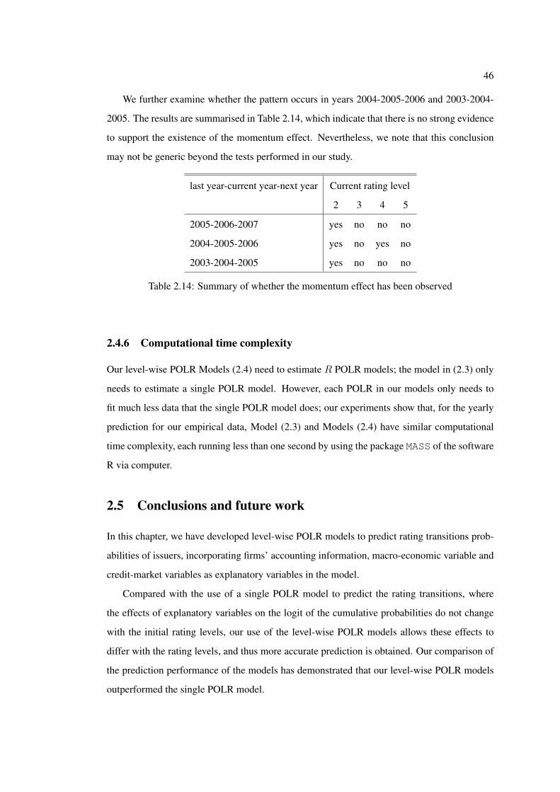
46

We further examine whether the pattern occurs in years 2004-2005-2006 and 2003-2004-

2005. The results are summarised in Table 2.14, which indicate that there is no strong evidence

to support the existence of the momentum effect. Nevertheless, we note that this conclusion

may not be generic beyond the tests performed in our study.

last year-current year-next year Current rating level

2 3 4 5

2005-2006-2007 yes no no no

2004-2005-2006 yes no yes no

2003-2004-2005 yes no no no

Table 2.14: Summary of whether the momentum effect has been observed

2.4.6 Computational time complexity

Our level-wise POLR Models (2.4) need to estimate R POLR models; the model in (2.3) only

needs to estimate a single POLR model. However, each POLR in our models only needs to

fit much less data that the single POLR model does; our experiments show that, for the yearly

prediction for our empirical data, Model (2.3) and Models (2.4) have similar computational

time complexity, each running less than one second by using the package MASS of the software

R via computer.


In this chapter, we have developed level-wise POLR models to predict rating transitions prob-

abilities of issuers, incorporating firms’ accounting information, macro-economic variable and

credit-market variables as explanatory variables in the model.

Compared with the use of a single POLR model to predict the rating transitions, where

the effects of explanatory variables on the logit of the cumulative probabilities do not change

with the initial rating levels, our use of the level-wise POLR models allows these effects to

differ with the rating levels, and thus more accurate prediction is obtained. Our comparison of

the prediction performance of the models has demonstrated that our level-wise POLR models

outperformed the single POLR model.

47

Moreover, the parameter-estimation results obtained by applying our models to empirical

data have indicated that the firm-specific variables, in particular the variables containing current

operational profitabilities and market leverage of the firm, explained the bulk of the rating

transitions. Macro-economic and credit market variables did not show strong impact on the

rating transitions in this study.

Finally, we have examined the momentum effect in the rating transitions (i.e. downgrading

is more likely followed by another downgrading). The results did not show strong evidence in

our study to support the existence of such an effect.

For future extensions of our models, it may be helpful to investigate a more sophisticated

version of the models, such as adding random effects into the current models. Kim and Sohn

(2008) develop a random-effects model by assigning Dirichlet prior distributions to the cu-

mulative probabilities P (Yt ≤ r|Xt−1) on the left-hand side of Model (2.3) and thus using

Bayesian methods to estimate the transition matrix.

In our case, a random-effects model can be obtained by adding firm-dependent random

effects γc (for firm c) to the right-hand side of Model (2.4), leading to

logit{P (Yt,c ≤ r|Xt−1,c, Yt−1,c = i)} = αi,r − βTi Xt−1,c − γc . (2.7)

Furthermore, more effects such as industry-dependent random effects and year-dependent ran-

dom effects can also be added to the right-hand side of Model (2.7). The random effects can

be assumed to be mutually independent. Let Yt,g,cg be the rating of firm c in industry g at time

t with the industry-dependent random effects ϕg and the year-dependent random effect ηt. The

model (2.7) becomes

logit{P (Yt,g,cg ≤ r|Xt−1,g,cg , Yt−1,g,cg = i)} = αi,r − βTi Xt−1,g,cg − γc − ϕg − ηt , (2.8)

where g = 1, . . . , G, the number of firms in industry group g is ng, and cg = 1, . . . , ng. We

can assume ϕg ∼ N(0, σ2g), γc ∼ N(0, σ2

c ) and ηt ∼ N(0, σ2t ), and assume that the random

effects are mutually independent.

However, according to Professor Brian Ripley, the Professor of Applied Statistics at the

University of Oxford, there is no reliable way to fit such a model and even no package in

R available for this undertaking. He suggested using Markov chain Monte Carlo (MCMC)

methods. A candidate software for this is WinBUGS.

Chapter 3

Accounting-based and market-based

models for credit risk

3.1 Introduction

3.1.1 Background

In this chapter we compare the performance of the two main categories of models for the

explanation and prediction of credit risk. These two categories are called accounting-based

models and market-based models, respectively.

There is a long tradition of the use of accounting variables to explain and predict credit

risk. The main early contribution in this area is Altman’s Z-score that was originated in the

1960s, and since then methodology has been developed and refined in subsequent generations

of accounting-based scoring models (Altman et al., 1977; West, 1985; Platt and Platt, 1991;

Altman and Saunders, 1998). However, this type of models is often criticised as lacking a solid

theoretical underpinning (Agarwal and Taffler, 2008).

In the 1970s, Black, Scholes, Merton and others developed the contingent claims approach

to modelling the liabilities of the firm. Merton (1974) is the seminal contribution in the anal-

ysis of defaultable bonds by means of a “structural model”, driven by assumptions about the

stochastic process of the firm’s assets as well as information about the terms and conditions of

the firm’s liabilities (e.g. coupon, leverage and term). In contrast to the accounting-based scor-

ing models, the implementation of structural models typically makes use of market information,

most notably stock market prices. The market-based structural approach is the cornerstone of

48

49

the KMV model, which becomes popular in banks and financial institutions because of its the-

oretical grounding and its use of up-to-date market information. As this approach considers the

capital structure of the firm, i.e. the assets value and debts value, it is called “structural model”.

Since the 1990s, another approach to tackling credit risk has appeared. This approach

assumes that the firm’s default time is driven by the default intensity based on the market prices

of credit securities. As this approach purely reduces all information to latent states variables, it

is called “reduced-form model”. Reduced-form models have merit of computational tractability

and have proved very useful in the relative pricing of redundant assets. However, the lack of

easy interpretation of the latent variables and the difficulty in identifying a stable process to

characterise their time-series behaviour have meant that they are not widely viewed as a solid

basis for credit risk prediction. For this reason in our research we focus on the models that

relate credit risk to observable variables, which are easier to interpret.

Market-based structural models are based on a clear interpretation of the credit event,

namely the bankruptcy process. The variables in market-based models can be regarded as

the main indicators of financial distress. Meanwhile, the variables that typically are used in

accounting-based credit models arguably are also salient indicators of distress. Accounting-

based models make use of variables derived from firm’s financial reports: balance sheets, in-

come statements and cash-flow statements. Since information from these financial reports re-

flects the recently-past performance of the firm, the accounting-based models may be regarded

as a backward-looking vision of the creditworthiness for the firm. In contrast, the concept of

the market-based models is based on the evolution of the market value of assets. The market

value of assets, through a channel of the market value of equity, usually reflects the view of

market participants on the future performance of the firm. Therefore the information used in

the market-based models is normally regarded as a forward-looking indicator of the creditwor-

thiness for the firm.

In this context, we are interested in finding whether these two sets of information (models)

have the same performance in the explanation and prediction of credit risk. If their perfor-

mances differ, we are then interested in figuring out which of them will be the most useful

in volatile periods of heightened systemic instability or at turning points of credit cycles. In

particular, we are interested in knowing which would have proved to be more reliable in the

recent financial crisis period. Such a period is likely to reveal structural instability of models

as manifested, for example, by significant changes in sensitivities to explanatory variables.

50

A new contribution of this chapter is as follows: We first divide our sample period into

a pre-crisis period and a post-crisis period, then examine the difference in explanatory and

predictive abilities of credit risk models between the pre-crisis and post-crisis periods. This

examination is undertaken for each of the accounting-based models, market-based models and

their combined comprehensive models. That is, our investigation lays emphasis on major cycli-

cal turning points and crises. To our best knowledge, this has not been found in the literature.

3.1.2 Related work and executive summary

The literature on performance comparison between the market-based models and the accounting-

based models is limited, as noted in Agarwal and Taffler (2008). Motivated by this, Agarwal

and Taffler (2008) find that the two models capture different aspects of bankruptcy risk. Based

on the UK data they find that there is little difference in their predictive ability. Das et al. (2009)

provide evidence on the US market. They find that the accounting-based model performs com-

parably to the market-based model, and the combination of the two sources of information

performs better than either of the two models.

In this chapter we build on the methodology of Das et al. (2009) to study the relative perfor-

mance of the accounting-based and market-based credit risk models as well as a comprehensive

model which includes both types of information. We apply this to an unbalanced panel of ob-

servations on the credit default swap (CDS) spreads for North American non-financial firms

between 2004 to 2011. The CDS spreads are a good proxy for credit risk, in terms of the

continuity of the CDS data in contrast to the dichotomy of the default data, and their market

perception in contrast to that of the rating data (Das et al., 2009). Because the CDS markets

are standardised and are typically more liquid than the underlying bonds and notes, and be-

cause they are less affected by tax considerations, they are widely regarded as a relatively pure

indicator of a firm’s financial distress.

We separate our sample into two sub-samples: pre-crisis and post-crisis. In September

2008, Lehman Brothers collapsed. This bankruptcy is widely viewed as the watershed event

beyond, which the entire financial system entered a period of crisis thus provoking wide-spread

bankruptcies, financial distress and a large global recession. Therefore, we choose the third

quarter of 2008 as a break-point for the crisis.

We investigate the performance of an accounting-based model, a market-based model and

51

a comprehensive model, for each of the sub-samples representing for the market conditions

before the Lehman Brothers’ failure and after its failure, respectively.

We find that, in the pre-crisis sample, there is little difference in fit of the two basic models,

i.e. the accounting-based and the market-based. The accounting-based variables are able to

explain 74% of the variation of the CDS rates, while the market-based variables can explain

72% of the variation of the CDS rates. These results are consistent with the findings in Agarwal

and Taffler (2008). We also find that the combination of both accounting-based and market-

based variables is able to explain 77% of the variation of the CDS rates. Furthermore, most

of the variables entering the two basic models remain significant in the comprehensive model.

Hence the accounting information and the market information are complementary. When we

apply the same methodology to the post-crisis period we find similar results: the explanatory

powers of the two basic models are comparable, and the performance is improved when the

two sources of information are combined.

When comparing the results for the pre-crisis sample versus the post-crisis sample, we find

that the explanatory power of the variables decreased. For example, for the comprehensive

models, from the before-crisis period to the after-crisis periods, the adjusted R-squared falls

from 77% to 62%. This may reflect the increased volatility in latent factors that has not been

captured by our accounting and market variables. One such factor could be the liquidity risk

predominating in the financial sector during the crisis period. Focusing on the banking sectors,

Gefang et al. (2011) suggest the importance of the liquidity risk relative to the credit risk to

the financial crisis in explaining the LIBOR-OIS (overnight index swap) rate. They find that,

particularly at the 1 month and 3 month terms, the role of the liquidity risk is much more

important than that of the credit risk. Alternatively, the decline in the model fit may reflect an

increase in the sensitivity of the CDS pricing to the perceived counter-party risk in these OTC

derivatives contracts.

While the explanatory powers of the accounting-based and market-based models are com-

parable in both the pre-crisis and post-crisis periods, some of the results suggest that the

accounting-based model is susceptible to structural instability. Our market-based model is

more parsimonious. It uses three explanatory variables versus thirteen variables for our accounting-

based model. Furthermore, there is considerable change between the pre-crisis and post-

crisis subsamples in the patterns of sign and significance of the estimated coefficients in the

accounting-based model.

52

We further establish one-quarter predictive models based on the pre-crisis subsample, and

use these models to predict the one-quarter ahead CDS spreads for the post-crisis period. We

calculate the mean squared prediction errors (MSE) across firms for each quarter in the post-

crisis period. A large MSE would indicate a greater change of economy from the pre-crisis

period.

We find that the MSE in the second quarter 2010 is the highest. This indicates that in the

first quarter of 2010 the economic situation is significantly different from that in the pre-crisis

period. Moreover, we find that overall the comprehensive model performs the best in cross-

sectional models for the prediction of distress. In addition, we find that, compared with the

accounting-base model, the market-based model does not always perform better in prediction.

When we compare the predictive performance of the cross-sectional models with that of the

autoregressive time-series (AR) models of the CDS spreads, we find that the latter outperforms

the former. This could be due to the fact that: 1) although the cross-sectional models are

comprehensive, they still miss certain variables affecting the variation of the CDS spreads; and

2) the error terms in the cross-sectional models might be correlated. Therefore, we investigate

the autocorrelation in the error terms and find that indeed the autocorrelation presents there.

In order to alleviate the impact of the autocorrelation on the model inference, we incorporate

lagged dependent variables (LDV), i.e. the lagged log CDS spreads, into the cross-sectional

models. The estimation results show that the addition of the LDV improves the model greatly

in terms of explanatory power (higher the adjusted R2) and predictive power (lower MSE) for

all the models in both pre-crisis and post-crisis periods.

In short, from our studies we observe the following two patterns. First, compared to the

accounting-based model and the comprehensive model, the market-based model performs the

best in the explanation of the CDS spreads, in the sense of having a comparable explanatory

power and being more parsimonious. Second, if we purely look for an optimal prediction of

the CDS spreads, we find that an AR time-series model of the CDS spreads outperforms the

cross-sectional models.

The remaining sections are organised as follows. Firstly, we introduce credit default swap

and its pricing formula. Secondly, we describe the data and the construction of variables.

Thirdly, we establish models and present the estimation results for each of the sample periods.

Fourthly, we carry out comparison of the performance of the predictive models. Fifthly, we

check for autocorrelation of the error terms and present the results for the models including the

53

LDV, and finally we conclude on the findings.

3.2 Credit default swap and its pricing model

Although the recent growth of the credit derivatives market has been concentrated on more

sophistic structured products, such as the collateralised debt obligations (CDOs), the credit

default swap (CDS) is still standing the largest position among other credit derivatives products.

The CDS market provides a relatively good platform to study the credit default risk, because a

credit default swap is seen as a purer credit indicator than a corporate bond.

A credit default swap is a bilateral swap contract between a protection buyer and a pro-

tection seller, against the credit default risk of financial securities of a reference entity. It can

also be regarded as a far out-of-the-money put option with the reference event of default: the

protection buyer has the right to sell the securities of the reference entity to the protection seller

in the event of default.

According to the contract, the protection buyer pays a periodic fee to the seller either at the

time of default or at the expiration time of the contract, whichever is the first; and the protection

seller promises to make a payment in the event of default of the reference entity. The periodic

fee, also called default risk price, with a fixed rate, is often referred to as credit default swap

spread. Following Berndt et al. (2005), the pricing formula for the CDS spreads is derived as

the following.

The risk-neutral probability of the firm surviving to T conditional on survival to t, under

the doubly stochastic assumption, is given as

p∗(t, T ) = EQ[e−∫

Tt λQ(u)du|Ft] . (3.1)

The CDS provides an insurance against potential loss due to the risk of default of a ref-

erence entity, hence the market value of the payment by the protection seller if default occurs

before the payment date tn is given by

h(t, s) = EQ[δ(t, τ)W sτ 1{τ≤tn)}|Ft] , (3.2)

where the default-free market discount factor δ(t, τ) is given as EQt [e

−∫ Tt r(u)du] and is as-

sumed to be independent of the default time under the probability measure. If default occurs

at time τ , the payment W sτ at the default time adjusted by accrued premium since last payment

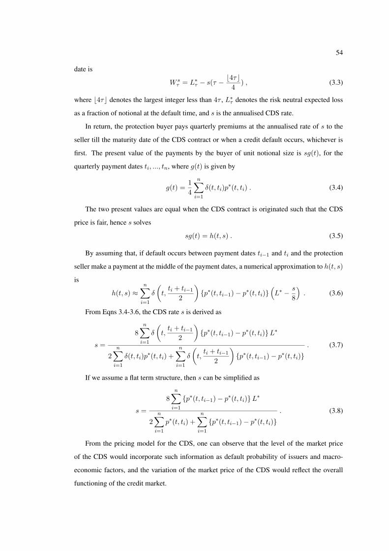
54

date is

W sτ = L∗

τ − s(τ − ⌊4τ⌋4

) , (3.3)

where ⌊4τ⌋ denotes the largest integer less than 4τ , L∗τ denotes the risk neutral expected loss

as a fraction of notional at the default time, and s is the annualised CDS rate.

In return, the protection buyer pays quarterly premiums at the annualised rate of s to the

seller till the maturity date of the CDS contract or when a credit default occurs, whichever is

first. The present value of the payments by the buyer of unit notional size is sg(t), for the

quarterly payment dates ti, ..., tn, where g(t) is given by

g(t) =1

4

n∑i=1

δ(t, ti)p∗(t, ti) . (3.4)

The two present values are equal when the CDS contract is originated such that the CDS

price is fair, hence s solves

sg(t) = h(t, s) . (3.5)

By assuming that, if default occurs between payment dates ti−1 and ti and the protection

seller make a payment at the middle of the payment dates, a numerical approximation to h(t, s)

is

h(t, s) ≈n∑

i=1

δ

(t,ti + ti−1

2

){p∗(t, ti−1)− p∗(t, ti)}

(L∗ − s

8

). (3.6)

From Eqns 3.4-3.6, the CDS rate s is derived as

s =

8

n∑i=1

δ

(t,ti + ti−1

2

){p∗(t, ti−1)− p∗(t, ti)}L∗

2

n∑i=1

δ(t, ti)p∗(t, ti) +

n∑i=1

δ

(t,ti + ti−1

2

){p∗(t, ti−1)− p∗(t, ti)}

. (3.7)

If we assume a flat term structure, then s can be simplified as

s =

8

n∑i=1

{p∗(t, ti−1)− p∗(t, ti)}L∗

2

n∑i=1

p∗(t, ti) +

n∑i=1

{p∗(t, ti−1)− p∗(t, ti)}. (3.8)

From the pricing model for the CDS, one can observe that the level of the market price

of the CDS would incorporate such information as default probability of issuers and macro-

economic factors, and the variation of the market price of the CDS would reflect the overall

functioning of the credit market.

55

This observation motives us to set up two type of models. One is to use accounting-based

variables plus macro-economic variables, and the other is to use market-based variables plus

macro-economic variables. Including macro-economic variables in both types of the models

allows us to distinguish the performance of the accounting-based variables and the market-

based variables in indicating the default probability of issues and in explaining the CDS rate.

3.3 Data

3.3.1 Collection and merger of the data

Our firm-specific data consist of four types of data.

• Firstly, the CDS data are collected on Datastream from January 2003 to Dec 2011. In

detail, daily 1-, 2-, 3-, 5- and 10-year constant maturity spreads whose notional values

are dollar-denominated are selected. The daily data are transformed into quarterly data

by taking the spreads at the end of each quarter.

• Secondly, the accounting data are collected on Compustat (North America Fundamentals

Quarterly) from the first quarter of 2003 to the fourth quarter of 2011, in which the

financial firms have been excluded.

• Thirdly, the daily share prices are collected from CRSP.

• Fourthly, the S&P domestic long-term issuer credit rating is collected from Compustat.

The CDS sample and the accounting data are merged by Ticker names. The merged sample

is further refined by requiring availability of at least 50 trading days equity returns prior to the

end of each quarter. After data processing, the firm-quarter data in the sample ranges from the

first quarter of 2004 to the fourth quarter of 2011.

Note that the CDS data on Datastream contain spreads from two data providers: Credit

Market Analysis (CMA) and Thomas Reuters (TR). CMA provides the CDS data starting from

January 2003 until September 2010, after then the CMA CDS data are restricted with an aca-

demic license. Hence since October 2010, TR has become the unique data source available

with the academic license. We combine the data from the two sources by integrating the CMA

entity mnemonics with the TR CDS mnemonics. Often the single CMA entity mnemonics can

be mapped to several TR CDS mnemonics with different restructuring type. In such cases, we

56

choose the restructuring type XR (No restructuring) from the TR data because of its common

use in the US region1.

Our macro-economic data include the following.

• 3-month constant maturity US Treasury bill rate from the website of U.S. Department of

the Treasury

• Monthly S&P 500 index level from the website of Standard and Poor’s

• Monthly average value-weighted returns for 17-industry portfolios from Fama-French’s

Data Library

Other related data, used to assist the construction of the explanatory variables, are listed as

follows.

• The industry definitions for 17-industry portfolios from Fama-French’s Data Library.

According to the definitions, we assign the industry to each firm in the sample by using

their Compustat SIC codes. (This is consistent to the industry definitions, where the

Compustat SIC code is applied; only when it is missing, the CRSP SIC code is used

instead. Das et al. (2009) use the CRSP SIC code.)

• The Consumer Price Index on all urban consumers (all items with the period 1982-1984

as a base), from the website of the Bureau of Labor Statistics of U.S. Department of

Labor.

• One year Treasury constant maturity rate from Board of Governors of the Federal Re-

serve System.

3.3.2 Construction of the explanatory variables

A summary of all the explanatory variables and their expected relationship with CDS (sign

displayed as a proxy) are listed in Table 3.1.

3.3.2.1 Accounting-based variables

From the collected accounting data, we construct 10 variables: size, roa, incgrowth, interest

coverage (split into c1–c4), quick, cash, trade, salesgrowth, booklev and retained.1See Thomas Reuters CDS–FAQ from data sources on Datastream

57

Explanatory variable Description Sign

Accounting-based variables

size Deflated assets -

- Profitability

roa Return on assets -

incgrowth Income growth -

c1 Interest coverage ∈ [0,5) -



c4 Interest coverage ∈ [20, 100] -

- Financial liquidity

quick Quick ratio -

cash Cash to asset ratio -

- Trading account activity

trade Inventories to COGS ratio +

salesgrowth Sales growth -

- Capital structure

booklev Leverage ratio +

retained Retained earnings to assets ratio -

Market-based variables

DTD Distance to default -

ret Annualised prior 65-trading day equity returns -

sdret Annualised stdev of prior 65-trading day equity returns +

Macro-economic variables

r 3-month constant maturity T-bill rates -

snp Prior year returns of S&P500 -

indret Prior year returns in the same Fama-Fench industry -

Contract-specific variables

invgrade Equal to 1 for firm in investment grade, 0 otherwise -

seniority Equal to 1 for senior underlying debt, 0 otherwise -

maturity Maturity of CDS contract (1, 2, 3, 5, 10 years) +

Table 3.1: List of the explanatory variables

58

These variables represent the characteristics of firms such as profitability, financial liquid-

ity, trades, size and leverage. They are usually regarded reflecting creditworthiness of the firms,

and are broadly used in academic research, such as Campbell et al. (2008) and Das et al. (2009).

Size Size is the deflated total value of assets. It is constructed as Total Asset (Compustat item

ATQ) divided by the Consumer Price Index.

Profitability

• Return on assets (roa). It is constructed as Net Income (item NIQ) divided by Total

Asset.

• Net income growth. It is equal to the ratio of quarterly increase in Net Income over Total

Asset.

• Interest coverage. It is calculated as the sum of Pretax Income (PIQ) and Interest Expense

(XINTQ) divided by Interest Expense.

Financial liquidity

• Quick ratio. It is constructed as the difference of Current Assets (ACTQ) and Inventories

(INVTQ) divided by Current Liabilities (LCTQ).

• Cash to asset ratio. It is constructed as Cash and Equivalents (CHEQ) divided by Total

Assets.

Trade account activities Trade is calculated as Inventories divided by Cost of Good Sold

(COGSQ).

Sales growth Sales growth is obtained by using quarterly increase in Sales (SALEQ) divided

by last quarter Sales.

Leverage

• Booklev is calculated as the ratio of Total Liabilities (LTQ) to Total Assets.

• Retained is the Retained Earnings (REQ) over Total Assets.

59

As in Das et al. (2009), we adjust roa, sales growth, interest coverage and trades for seasonal

effects. That is, we use the trailing 1-year average of these variables in the models.

In particularly, before taking the trailing 1-year average for interest coverage ratio, we set

any negative ratio to zero and censor the ratio at 100 if they are greater than 100. This takes

into account the conjecture that: 1) a negative interest ratio should not last long and firm must

find a way to meet the interest expense; and 2) when the pre-tax income is much larger than

the interest expense, the magnitude of the difference would convey no additional information

on the firm’s creditworthiness.

Furthermore, we change the specification of the interest coverage ratio so as to consider

the shape of the non-linearity. The ratio is split into 4 variables c1it – c4it (Table 3.2) and the

coefficients will be determined in the models with other variables. The non-linearity would be

reflected in the estimated coefficients, i.e. the slope of interest ratio intervals.

c1it c2it c3it c4it

ICit ∈ [0, 5) ICit 0 0 0

ICit ∈ [5, 10) 5 ICit -5 0 0

ICit ∈ [10, 20) 5 5 ICit -10 0

ICit ∈ [20, 100] 5 5 10 ICit -20

Table 3.2: Transformation of interest coverage ratio

3.3.2.2 Market-based variables

We construct 3 market-based variables: DTD, ret and sdret.

The distance-to-default (DTD) concept is originated from Merton’s model and applied as

a cornerstone in Moodys’ KMV model. The DTD has advantages that it combines the market

value of assets, business risk and financial leverage into a single credit risk measure. The evi-

dence that the DTD outperforms accounting variables has been documented in several research

papers (Hillegeist et al., 2004).

The DTD can be calculated by solving for the asset value of firm V and its standard devia-

60

tion σV from a system of non-linear equations:

E = V N(d1)− e−rTFN(d2) ,

σE =V

EN(d1)σV ,

where E is the market value of the firm’s equity, F is the face value of the firm’s debt, r is the

instantaneous risk-free interest rate, N(·) is the cumulative distribution function for standard

normal distributed random variables, and

d1 =ln(VF ) + (r + 0.5σ2

V )T

σV√T

,

d2 = d1 − σV√T .

In the calculation, the market value of the firm’s equity is estimated as the multiplication

of the number of shares outstanding (Compustat item CSHOQ) and the end-of-quarter closing

stock prices (item PRCCQ). The face value of the firm’s debt is calculated by current liabilities

(item LCTQ) plus half of the long-term debt (item DLTTQ). The rate r is proxyed by the one-

year Treasury constant maturity rate at the end of each quarter; T is set to be 1 year as in

convention; σE is estimated by the standard deviation of the firm’s daily stock price returns for

trailing 65 trading days (∼ 1 quarter). As in Das et al. (2009) and other papers, we calculate

the DTD only for the quarter when at least prior 50 trading-day returns are available.

After obtaining the values of V and σV , we calculate the DTD as follows:

DTD =ln(VF ) + (µV − 0.5σ2

V )T

σV√T

,

where µV is estimated by the annualised mean equity returns on the prior 65 trading days.

3.3.2.3 Macro-economic and contract-specific variables

The 3-month constant maturity US Treasury bill (T-bill) rates are used as the measure of

macroeconomic conditions. If the T-bill rate is low, the credit default spread would be ex-

pected high. We use also the prior year returns in the same Fama-French industry where the

firm belongs to, in order to reflect the firm’s industry risk. Prior year returns on the S&P 500

index are also included.

For contract-specific variables, we set a dummy variable for seniority of the CDS contract.

The dummy variable is equal to 1 if the underlying debt of the contract is in seniority, and to 0

61

otherwise. In addition, we include the maturity of the CDS contract as a variable which takes

values of 1, 2, 3, 5 and 10. In normal cases and ceteris paribus, the longer the maturity, the

higher the CDS rate. This is due to the greater uncertainty in the credit risk for the longer-term

CDS contract. We also have a dummy, equal to 1 if the underlying debt of the contract carry

an investment grade and to 0 otherwise.

3.4 Empirical studies

We are interested in finding whether the accounting-based information/models and the market-

based information/models have the same performance in the explanation and prediction credit

risk. If their performances differ, which will be the most useful in volatile periods of heightened

systemic instability or at turning points of credit cycles? In particular, we are interested in the

relative reliability of these two sets of information/models for the recent crisis period.

To answer these questions, we investigate various models with the accounting-based vari-

ables, with the market-based variables and with both the accounting-based and market-based

variables. Furthermore, for each of the models, we will fit the model to two sets of data: one

dataset represents a relatively quiet market, and the other represents a relatively volatile market.

We partition samples into the pre-crisis sample and the post-crisis sample. We choose the

third quarter of 2008 as the cut-off quarters, taking into account the turmoil in the US when

Lehman Brothers failed in September 2008. That is, the data in a quarter prior the second

quarter of 2008 belong to the pre-crisis sample, while the data in a quarter after the third quarter

of 2008 are used for estimating the post-crisis models. The term of pre-crisis is interchangeably

used as before-crisis in the chapter; similarly, the post-crisis is interchangeably used with after-

crisis.

In total, our pre-crisis sample contains the data for 18 quarters from 2004Q1 to 2008Q2.

The post-crisis sample contains 14 quarters in total from 2008Q3 to 2011Q4. The descriptive

statistics for each sample are listed in Table 3.3.

3.4.1 Explanatory models

We set up three types of models:

• model 1: accounting-based models;

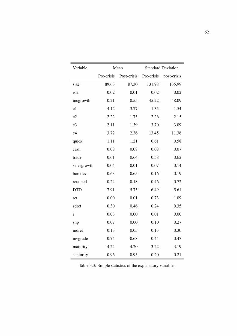
62

Variable Mean Standard Deviation

Pre-crisis Post-crisis Pre-crisis post-crisis

size 89.63 87.30 131.98 135.99

roa 0.02 0.01 0.02 0.02

incgrowth 0.21 0.55 45.22 48.09

c1 4.12 3.77 1.35 1.54

c2 2.22 1.75 2.26 2.15

c3 2.11 1.39 3.70 3.09

c4 3.72 2.36 13.45 11.38

quick 1.11 1.21 0.61 0.58

cash 0.08 0.08 0.08 0.07

trade 0.61 0.64 0.58 0.62

salesgrowth 0.04 0.01 0.07 0.14

booklev 0.63 0.65 0.16 0.19

retained 0.24 0.18 0.46 0.72

DTD 7.91 5.75 6.49 5.61

ret 0.00 0.01 0.73 1.09

sdret 0.30 0.46 0.24 0.35

r 0.03 0.00 0.01 0.00

snp 0.07 0.00 0.10 0.27

indret 0.13 0.05 0.13 0.30

invgrade 0.74 0.68 0.44 0.47

maturity 4.24 4.20 3.22 3.19

seniority 0.96 0.95 0.20 0.21

Table 3.3: Simple statistics of the explanatory variables

63

• model 2: market-based models;

• model 3: comprehensive models.

For each type of models, we fit the models to both the pre-crisis and post-crisis samples.

It can be observed from Table 3.3 that the standard deviations are large for some variables.

Therefore, in order to avoid undesirable effects of extreme values on the model estimation, we

winsorise some variables by their 5% and 95% quantiles. That is, the data value greater than

the 95% quantile is set to be the 95% quantile and the data value smaller than the 5% quantile

is set to be the 5% quantile. The variables winsorised include CS (denoting the CDS spreads),

size, roa, incgrowth, quick, cash, trade, salesgrowth, booklev, retained, DTD, ret, sdret, r, snp

and indret. We also take logarithm for size considering its relatively large magnitude to other

variables.

3.4.1.1 Accounting-based models (M1)

The specification for the accounting-based model follows Eqn (3.9). The estimation results of

the model can be found in the second column (Column 2) and the third column (Column 3) of

Table 3.4, for the before-crisis and after-crisis periods, respectively.

ln(CSit) =α+ β1sizeit + β2roait + β3incgrowthit + β4c1it + β5c2it + β6c3it

+ β7c4it + β8quickit + β9cashit + β10tradeit ++β11salesgrowthit

+ β12booklevit + β13retainedit + β14rit + β15snpit

+ β16indretit + β17invgradeit + β18maturityit + β19seniorityit + ϵit .

(3.9)

Column 2 in Table 3.4 provides the results for the pre-crisis sample. Some patterns can be

observed as follows.

• Firstly, all variables have significant effects except for quick, cash, salesgrowth and book-

lev. For these significant variables, the signs of estimated coefficients are all consistent

to our expectation except for trade. That is, amongst the accounting-based variables,

the size of firms (Log of assets), roa, income growth rate, interest coverage and retained

earnings have a negative relationship to the CDS spreads.

• Secondly, the nonlinearity of interest coverage is reflected via the different values of

the estimated coefficients and the decreasing significance (as the t-statistics decreases)

64

Variable Acc-based model Market-based model Comprehensive modelBefore After Before After Before After

(Intercept) 6.41 ∗∗∗ 5.77 ∗∗∗ 5.88 ∗∗∗ 5.06 ∗∗∗ 6.39 ∗∗∗ 5.12 ∗∗∗

(110.38) (93.43) (154.95) (126.9) (106.51) (77.16)Log of assets -0.21 ∗∗∗ -0.13 ∗∗∗ -0.15 ∗∗∗ -0.07 ∗∗∗

(-35.11) (-20.41) (-25.17) (-11.2)roa -7.05 ∗∗∗ -9.68 ∗∗∗ -4.43 ∗∗∗ -4.71 ∗∗∗

(-10.13) (-14.87) (-6.76) (-7.47)incgrowth -0.38 -2.62 ∗∗∗ -1.00 ∗ -1.56 ∗∗∗

(-0.88) (-6.10) (-2.48) (-3.82)c1 -0.09 ∗∗∗ -0.06 ∗∗∗ -0.09 ∗∗∗ -0.05 ∗∗∗

(-14.09) (-10.29) (-15.33) (-9.00)c2 -0.02 ∗∗∗ -0.05 ∗∗∗ -0.03 ∗∗∗ -0.05 ∗∗∗

(-6.26) (-10.81) (-8.07) (-11.96)c3 -0.01 ∗∗∗ 0.01 ∗∗∗ -0.01 ∗∗∗ 0.01 ∗

(-4.03) (4.54) (-4.51) (2.42)c4 0.00 ∗∗ 0.00 ∗ 0.00 ◦ 0.00 ∗∗∗

(-2.94) (-2.50) (-1.68) (-3.29)quick 0.02 -0.04 ∗ 0.06 ∗∗∗ -0.02 ◦

(1.21) (-2.46) (5.07) (-1.79)cash 0.15 1.02 ∗∗∗ -0.12 0.77 ∗∗∗

(1.57) (9.36) (-1.34) (7.44)trade -0.18 ∗∗∗ -0.07 ∗∗∗ -0.13 ∗∗∗ -0.05 ∗∗∗

(-14.97) (-5.75) (-11.16) (-3.86)salesgrowth -0.22 0.94 ∗∗∗ -0.45 ∗∗∗ 0.36 ∗∗

(-1.55) (6.90) (-3.33) (2.77)booklev -0.03 0.34 ∗∗∗ -0.07 ◦ 0.40 ∗∗∗

(-0.72) (6.98) (-1.67) (8.58)retained -0.34 ∗∗∗ -0.35 ∗∗∗ -0.19 ∗∗∗ -0.23 ∗∗∗

(-13.45) (-13.02) (-7.96) (-8.8)DTD -0.10 ∗∗∗ -0.06 ∗∗∗ -0.07 ∗∗∗ -0.04 ∗∗∗

(-52.63) (-26.14) (-37.51) (-16.70 )ret 0.43 ∗∗∗ 0.21 ∗∗∗ 0.30 ∗∗∗ 0.09 ∗∗∗

(32.39) (17.88) (23.93) (7.94)sdret -0.31 ∗∗∗ 1.03 ∗∗∗ 0.06 0.88 ∗∗∗

(-6.53) (23.95) (1.25) (21.01)r -14.91 ∗∗∗ -18.72 ∗∗∗ -13.41 ∗∗∗ -20.45 ∗∗∗ -13.09 ∗∗∗ -15.96 ∗∗∗

(-38.64) (-9.56) (-33.81) (-10.49) (-35.87) (-8.48)snp -1.72 ∗∗∗ -0.45 ∗∗∗ -0.66 ∗∗∗ 0.53 ∗∗∗ -0.96 ∗∗∗ 0.21 ∗∗

(-26.23) (-6.74) (-9.75) (7.77) (-15.14) (3.13)indret -0.46 ∗∗∗ -0.57 ∗∗∗ -0.73 ∗∗∗ -0.53 ∗∗∗ -0.59 ∗∗∗ -0.40 ∗∗∗

(-9.82) (-9.16) (-15.67) (-8.52) (-13.02) (-6.61)invgrade -1.10 ∗∗∗ -0.75 ∗∗∗ -1.36 ∗∗∗ -0.91 ∗∗∗ -0.96 ∗∗∗ -0.62 ∗∗∗

(-73.49) (-50.65) (-106.1) (-70.57) (-66.05) (-42.76 )maturity 0.15 ∗∗∗ 0.08 ∗∗∗ 0.15 ∗∗∗ 0.08 ∗∗∗ 0.15 ∗∗∗ 0.08 ∗∗∗

(101.25) (51.80) (99.15) (51.29) (108.13) (54.63)seniority -0.27 ∗∗∗ -0.12 ∗∗∗ -0.29 ∗∗∗ -0.15 ∗∗∗ -0.24 ∗∗∗ -0.11 ∗∗∗

(-11.1) (-4.88) (-11.89) (-5.79) (-10.63) (-4.48)

R2 73.53% 58.18% 72.15% 57.34 % 76.77 % 62.46Adj. R2 73.50% 58.13 % 72.13% 57.32 % 76.74% 62.41N 16103 15922 16103 15922 16103 15922

Table 3.4: Estimation results. (The numbers in bracket are t-statistics. The significance codes:

0 ∗ ∗ ∗; 0.001 ∗∗; 0.01 ∗ ; 0.05 ◦)

65

from c1 to c4, which confirms the conjecture that an increased value of interest coverage

provides little additional information to the firm’s performance.

• Thirdly, as expected, the macro-economic variables are all statistically significant and

are negatively related to the CDS spreads, indicating the sensitivity of the CDS spreads

to the macro-economic environment.

• Finally, regarding the contract-specific variables, both maturity and seniority are signif-

icant and have the expected signs: a positive sign for maturity and a negative sign for

seniority.

Column 3 of Table 3.4 presents the results for the post-crisis period. For comparison be-

tween the model for the before-crisis period and the model for the after-crisis period, we iden-

tify changes in significance and sign of the estimated coefficients and in the adjusted R2 of the

models, from the before-crisis to the after-crisis. Based on the comparison, some interesting

patterns of change and their implications are discussed as follows.

• The nonsignificant variables (quick, cash, sales growth and booklev) in the pre-crisis

model become significant. This indicates that the financial liquidity factor (represented

by quick and cash ratio) is more relevant to the firm’s creditworthiness in a crisis market

than in a relative quiet market, and the liquidity variation plays a more important role in

affecting the credit spread widening in the financial crisis.

• As for the changes in the sign, the sales growth changes sign, from negative to positive.

Although the negative sign is not consistent to the expected univariate relationship, this

is also observed in Das et al. (2009). The book leverage changes sign, from negative to

positive; the quick ratio changes sign, from positive to negative; both are consistent to

our expectation. Cash is significant in the after-crisis period, and in a positive association

with the CDS spreads. This is somewhat counterintuitive as one would expect the more

cash holding the lower CDS rate. This could be explained by the fact that the firm prefers

holding cash to making investment in a crisis period; and the market views such holding-

cash behaviour as a temporary decision of the firm. The decision benefits the short-term

liability, but is not good in meeting the long-term liability.

• Further comparing the models on the pre-crisis and post-crisis periods, we find that the

adjusted coefficient of determination R2 decreased by 26% from 74% to 58%, indicating

66

that the explanatory power of the model decreased. This may be due to the increased

volatility in latent factors that have not been captured by our accounting and market

variables. One such factor could be the liquidity risk predominating in the financial

sector during the crisis time period. The liquidity risk in financial sectors eventually

spreads out to other industries.

3.4.1.2 Market-based models (M2)

The specification of the market-based model (Model 2) follows Eqn (3.10). Besides the market-

based variables, here we also include the macro-economic variables as well as the contract-

specific variables.

ln(CSit) =α+ β1DTDit + β2retit + β3sdretit

+ β4rit + β5snpit + β6indretit + β7invgradeit

+ β8maturityit + β9seniorityit + ϵit .

(3.10)

Columns 4-5 in Table 3.4 provide the estimation results for the pre-crisis period and the

post-crisis period, respectively.

All the market variables are significant in both the post-crisis and pre-crisis periods. The

macro-economic and contract-specific variables are also all significant in both periods and

display the same pattern of signs as when they appeared in the accounting-based model. The

overall fit of the market-based model is very close to that obtained in the accounting-based

model in both the pre-crisis and post-crisis periods. Given that the market-based model is

more parsimonious, with three market variables compared to thirteen accounting variables,

this perhaps is surprising and may be taken as a strength of this model. While the sign of the

coefficient on the variable sdret does switch from negative in the pre-crisis sample to positive

in the post-crisis period, this does appear more stable than in the case of the accounting-based

model where there are four changes of sign.

67

3.4.1.3 Comprehensive models (M3)

Putting accounting and market variables together as well as the macro-economic and contract-

specific variables, we set up a comprehensive model as in Eqn (3.11).

ln(CSit) =α+ β1sizeit + β2roait + β3incgrowthit + β4c1it + β5c2it + β6c3it

+ β7c4it + β8quickit + β9cashit + β10tradeit + β11salesgrowthit

+ β12booklevit + β13retainedit + β14DTDit + β15retit + β16sdretit

+ β17rit + β18snpit + β19indretit + β20invgradeit


(3.11)

The estimation results are listed in Columns 6-7 of Table 3.4. Some thought-provoking

patterns can be observed from the comparison between the comprehensive models and the two

basic models. Examples include the following.

• We find that, most of the variables, that are statistically significant in the two basic mod-

els, remain statistically significant in the comprehensive model. This indicates that the

two sets of information, the accounting-based and the market-based, are complemen-

tary. This pattern is reliable for both periods. We note that variables used in estimating

DtD are then used again in a regression to explain the size of the CDS premium (credit

spread). We have followed the wide-spread practice of implementing distance to default

using the historical distribution of firm value. This can be justified by the empirical na-

ture of our model. In applications of the Merton model for pricing purposes distance

to default theoretically should be measured from the risk neutral distribution. In prin-

ciple, this might give rise to different results in empirical applications such as our own;

however, we have not explored this here.

• As for the explanatory power, the comprehensive models get improved in both the pre-

crisis and post-crisis periods, compared with the basic models. For example, for the

pre-crisis period, the accounting-based variables are able to explain 74% of the variation

of the CDS rates, the market-based variables can explain 72%, while the combination of

both accounting-based and market-based variables is able to explain 77%. These results

are consistent with the findings in Agarwal and Taffler (2008).

• Similarly to that for the two basic models, we observe that the adjusted R2 falls from

77% to 62% from the pre-crisis period to the post-crisis period. As discussed before, this

68

may reflect the increased volatility in latent factors that has not been captured by our ac-

counting and market variables. One such factor could be the liquidity risk predominating

in the financial sector during the crisis period. Concentrating on financial sectors, Gefang

et al. (2011) suggest the importance of the liquidity risk relative to the credit risk on the

financial crisis. They find that, for short terms especially for the 1 month and 3 month

terms, the role of the liquidity risk is much more important. Since our accounting and

market variables are designed to capture the credit risk rather than the liquidity risk, we

would expect our model is better fit for the long-term CDS spreads than for short-term

ones. To confirm this we fit the comprehensive models to the 1-year CDS spreads and to

the 5-year CDS spreads respectively, and we find that the adjusted R2 for the former is

0.58 while for the latter is 0.64. Alternatively, the decline in the model fit may reflect an

increase in the sensitivity of the CDS pricing to the perceived counter-party risk in these

OTC derivatives contracts.

3.4.2 Predictive models

The focus so far has been on the ability of alternative sets of information to account for the

cross-sectional variation of the CDS spreads across different firms. In practical applications

we might consider the use of these models in portfolio choice. For example, the models might

be used to construct portfolios of over-valued and under-valued contracts which could be used

to take convergence type risk-arbitrage trades. Or the models might be used to extrapolate

in cross-section, for example, in pricing CDS on a name that is not currently quoted in the

market. However, for predictions over time, the models as specified may need to be adapted.

The accounting-based, market-based and comprehensive models that we have considered so far

all use contemporaneous explanatory variables as in Agarwal and Taffler (2008) and Das et al.

(2009). To make time-series predictions one could attempt to forecast the explanatory variables

and find the implied forecast. Given the number of explanatory variables involved, however,

this seems unlikely to be the most practicable approach in most contexts. Consequently, we

develop predictive models based on lagged variables.

Specifically we will use predictive regression models estimated on the data from the pre-

crisis period to predict the CDS spreads for the post-crisis period. In general, we regress

log(CS) on the one-quarter lagged explanatory/predictor variables. We use various combina-

69

tions of lagged predictors for the models M1-M3, as illustrated below:

Pred.M1 : CDSt = acct−1 + + macrot−1 + contractt ;

Pred.M2 : CDSt = markett−1 + macrot−1 + contractt ;

Pred.M3 : CDSt = acct−1 + markett−1 + macrot−1 + contractt ,

where acct−1, markett−1 and macrot−1 denote accounting-based, market-based and macro-

economic variables with a one-quarter lag, respectively.

In more detail, the predictive model 1 (Pred.M1) accounts for the lagged accounting and

macro-economic variables, as specified in Eqn (3.12):

ln(CSit) =α+ β1sizei,t−1 + β2roai,t−1 + β3incgrowthi,t−1 + β4c1i,t−1 + β5c2i,t−1

+ β6c3i,t−1 + β7c4i,t−1 + β8quicki,t−1 + β9cashi,t−1 + β10tradei,t−1

+ β11salesgrowthi,t−1 + β12booklevi,t−1 + β13retainedi,t−1

+ β14ri,t−1 + β15snpi,t−1 + β16indreti,t−1 + β17invgradei,t−1


(3.12)

In the predictive model 2 (Pred.M2), the market variables and macro-economic variables

are lagged by one quarter as in Eqn (3.13):

ln(CSit) =α+ β1DTDi,t−1 + β2reti,t−1 + β3sdreti,t−1



(3.13)

The predictive model 3 (Pred.M3) includes the lagged accounting, market and macro-

economic variables, as shown in Eqn (3.14):

ln(CSit) =α+ β1sizei,t−1 + β2roai,t−1 + β3incgrowthi,t−1 + β4c1i,t−1 + β5c2i,t−1

+ β6c3i,t−1 + β7c4i,t−1 + β8quicki,t−1 + β9cashi,t−1 + β10tradei,t−1

+ β11salesgrowthi,t−1 + β12booklevi,t−1 + β13retainedi,t−1

+ β14DTDi,t−1 + β15reti,t−1 + β16sdreti,t−1



(3.14)

70

Figure 3.1: Prediction mean squared errors

2008Q3 2008Q4 2009Q1 2009Q2 2009Q3 2009Q4 2010Q1 2010Q2 2010Q3 2010Q4 2011Q1 2011Q2 2011Q3 2011Q4

Pred.M1 0.85 1.71 1.28 0.99 1.00 0.82 0.84 1.90 0.83 0.56 0.50 0.47 1.33 0.62

Pred.M2 0.67 1.54 1.73 0.89 0.77 0.61 0.64 1.16 0.52 0.53 0.63 0.50 1.10 0.38

Pred.M3 0.70 1.48 1.16 0.84 0.90 0.73 0.65 1.22 0.49 0.48 0.59 0.47 1.17 0.44

AR.CDS 0.14 0.75 0.20 0.37 0.31 0.18 0.08 0.16 0.10 0.23 0.10 0.05 0.28 0.07

Table 3.5: Prediction mean squared errors

For these 3 cross-sectional predictive models, Figure 3.1 and Table 3.5 present the mean

squared errors (MSE) over all firms at each quarter for the post-crisis period. Specifically, the

prediction error is the logarithm of the ratio of the predicted spread to the observed spread.

If the MSE for quarter Q is large, it can be implied that the properties of the predictor

variables at Q− 1 are quite different from those in the pre-crisis period. That is, the economic

situation described by the variable spaces has changed from the pre-crisis period. On the other

end, if the MSE is small for quarter Q, then the economic status in quarter Q− 1 is similar to

that in the pre-crisis period.

From Figure 3.1 and Table 3.5 we can observe a number of interesting patterns.

• In all but three quarters the market-based model has a smaller prediction error than the

accounting-based model.

71

• The accounting-based, market-based, and comprehensive models all have very large

prediction errors in three periods— the immediate aftermath of Lehman Brothers in

2008Q4 and 2009Q1, in 2010Q2 when the fears of double-dip recession were great,

and in 2011Q3 when the euro crisis had reach alarming proportions.

• Some details of timing might suggest different relative strengths of different informa-

tion sources. As for Pred.M1, where only the accounting information and the macro-

economic information are lagged, we can observe that the MSE hits the highest in the

second quarter of 2010. Because of the one-quarter lag, the economic status explained

by the accounting variables refers to the first quarter of 2010. Hence this indicates that

the economic environment (expanded mainly by the accounting and macro-economic in-

formation) during the first quarter of 2010 is remarkably different on average from that

in the pre-crisis period. Therefore the quarter could be a time point that the economy is

enduring a potential transition.

• Throughout all the predictive models, Pred.M1, Pred.M2 and Pred.M3, we can observe

a common trend that the MSEs for the models start relatively low, increase in the forth

quarter of 2008, decrease back to the level of the third quarter of 2008 and hit a peak in

the second quarter of 2010. Since then, the MSEs continuously decline for 3 quarters.

The common trend indicates that there exists two stages. The first stage is from 2008Q3

to 2010Q1, where the economy behaviours were quite different from that in the pre-

crisis period. The second stage starts from 2010Q2 where the economy moved towards

the before-crisis level, a sign of potential recovery.

• Figure 3.1 also shows that overall the comprehensive model performs the best in the

cross-sectional prediction.

All these are comparisons of predictive versions of the cross-sectional models considered

so far. However, for pure predictions over time, it is interesting to compare these to a simple,

pure time-series model. We have estimated such a model as well. Specially, we set up a fourth-

order auto-regression model, as displayed in Eqn (3.15) for the CDS spreads over the pre-crisis

period, and then use the fitted model to obtain the predictive MSE for the post-crisis period.

ln(CSit) = α+β1 ln(CSi,t−1)+β2 ln(CSi,t−2)+β3 ln(CSi,t−3)+β4 ln(CSi,t−4)+ϵit (3.15)

72

The MSE for the AR benchmark model are presented in Figure 3.1 and Table 3.5. It is noted

that the AR time-series model outperforms all the cross-sectional models. In our opinion, there

may be two reasons for this phenomenon. First, there may be some omitted variables in the

cross-sectional models. Second, the variation of CDS rates may be driven by its own supply-

demand shocks, but such information is not able to be captured by the cross-sectional models.

If these omitted variables or shocks can be represented by persistent latent variables, this may

be reflected in autocorrelated residuals in the cross-sectional models, something that is not

typically considered in the previous literature. This motivates us to our further investigation in

Section 3.4.3.

3.4.3 Time-series models or cross-sectional models?

3.4.3.1 Autocorrelation check for the residuals

We examine the autocorrelation of the residuals that we obtained from the estimation for

Model 1, Model 2 and Model 3, presented in sections 3.4.1.1, 3.4.1.2 and 3.4.1.3, respec-

tively. We fit a fourth-order AR model to the residuals, taking into account possible seasonal

effects. That is, the model is set up as

Residit = α+ β1Residi,t−1 + β2Residi,t−2 + β3Residi,t−3 + β4Residi,t−4 + ϵit . (3.16)

The results are listed in Table 3.6, where resid.lag1-resid.lag4 denote the first-fourth orders

AR terms of the residuals. We see that there is a very large positive coefficient at first-order

lag for all the models in both the pre-crisis and post-crisis periods. However, the AR terms are

significant out to four lags. That is, all t-statistics are highly significant, at least at the 1% sig-

nificance level. We interpret this to be strong confirmation of our conjecture that there is some

persistent latent variable that has been omitted from the cross-sectional models. Therefore, we

alter the specification to take this into account.

Our approach is to include the lagged CDS spreads into the cross-sectional models. We are

expecting that the addition of lagged dependent variables will reduce the autocorrelation in the

residuals, and will improve the models’ performance in terms of explanatory power and pre-

diction power. Hence, on the basis of the accounting-based, market-based and comprehensive

models described in Section 3.4, we develop new models with additional 1-4 lags of the log

CDS spreads.

73

Variable Acc-based model Market-based model Comprehensive model

Before After Before After Before After

(Intercept) 0.04 0.02 0.03 0.01 0.04 0.01

11.91 5.63 7.50 2.79 10.22 3.33

resid.lag1 0.71 0.84 0.57 0.65 0.59 0.70

74.70 86.91 60.63 66.71 62.21 71.70

resid.lag2 0.08 -0.06 0.14 0.15 0.14 0.11

6.83 -4.66 13.19 12.68 12.94 9.00

resid.lag3 0.04 -0.07 0.05 -0.05 0.06 -0.06

3.05 -5.61 4.96 -4.01 5.11 -5.26

resid.lag4 0.02 0.14 0.06 0.09 0.03 0.09

2.10 15.82 6.06 10.12 2.83 10.27

R2 66.43% 70.02% 56.41% 66.57% 55.34% 65.62%

Adj R2 66.41% 70.01% 56.39% 66.55% 55.33% 65.60%

N 16103 15922 16103 15922 16103 15922

Table 3.6: Estimation results of the AR(4) models for residuals (The t-statistics are reported

below the coefficients)

74


(Intercept) 1.76∗∗∗ 1.12 ∗∗∗ 1.59 ∗∗∗ 0.57 ∗∗∗ 1.86∗∗∗ 0.68 ∗∗∗

(30.57) (22.37) (40.92) (16.22) (31.77) (13.71)size -0.03∗∗∗ -0.05 ∗∗∗ -0.02 ∗∗∗ -0.02∗∗∗

(-7.4) (-12.27) (-3.99) (-5.82)roa -2.00 ∗∗∗ -2.38∗∗∗ -1.09 ∗ -0.3

(-4.25) (-5.95) (-2.38) (-0.8)incgrowth -0.4 -3.19 ∗∗∗ -0.66 ∗ -2.06 ∗∗∗

(-1.36) (-11.98) (-2.33) (-8.4)c1 -0.02∗∗∗ 0.00 -0.02 ∗∗∗ 0.00

(-4.9) (-0.05) (-5.57) (1.09)c2 0.00 -0.01 ∗∗ 0.00 -0.01 ∗∗∗

(1.5) (-2.97) (0.18) (-5.97)c3 0.00 0.00 ∗∗ 0.00 0.00

(-1.29) (2.68) (-1.45) (0.12)c4 0.00 0.00 0.00 0.00

(-1.24) (1.04) (-0.85) (0.12)quick -0.01 -0.02 ∗ 0.01 -0.02 ∗∗

(-0.87) (-2.3) (0.61) (-2.97)cash -0.29∗∗∗ 0.1 -0.3 ∗∗∗ 0.12 ◦

(-4.24) (1.48) (-4.56) (1.87)trade -0.03∗∗∗ -0.01 -0.01 0.00

(-3.46) (-1.41) (-1.34) (-0.44)salesgrowth -0.29 ∗∗ 1.25∗∗∗ -0.3 ∗∗ 0.7 ∗∗∗

(-2.86) (14.8) (-3.07) (9.01)booklev 0.00 0.11 ∗∗∗ -0.02 0.1 ∗∗∗

(0.01) (3.63) (-0.77) (3.4)retained 0.02 -0.11 ∗∗∗ 0.05 ∗∗ -0.05 ∗∗∗

(1.19) (-6.44) (2.89) (-3.36)DTD -0.03∗∗∗ 0.00 -0.03∗∗∗ 0.00∗∗

(-20.25) (1.27) (-18.23) (2.79)ret 0.01 -0.17∗∗∗ 0.02 ◦ -0.17∗∗∗

(1.49) (-24.71) (1.94) (-24.59)sdret -0.15 ∗∗∗ 0.7 ∗∗∗ -0.07 ∗ 0.69 ∗∗∗

(-5.01) (28.04) (-2.2) (26.89)r -20.68∗∗∗ 0.71 -17.75∗∗∗ -1.12 -17.78∗∗∗ -2.75∗

(-42.78) (0.51) (-36.87) (-0.88) (-37.14) (-2.13)snp 1.12∗∗∗ -0.14∗∗ 1.12∗∗∗ 0.15 ∗∗∗ 1.05 ∗∗∗ 0.12∗∗

(15.09) (-3.29) (15.68) (3.67) (14.53) (2.91)indret -0.19∗∗∗ -0.35 ∗∗∗ -0.15∗∗∗ -0.03 -0.13∗∗∗ -0.05

(-5.63) (-9.21) (-4.85) (-0.73) (-3.97) (-1.5)invgrade -0.13 ∗∗∗ -0.13 ∗∗∗ -0.13∗∗∗ -0.1 ∗∗∗ -0.12 ∗∗∗ -0.07∗∗∗

(-9.83) (-12.69) (-10.57) (-11.05) (-9.63) (-7.36)maturity 0.02 ∗∗∗ 0.02 ∗∗∗ 0.01∗∗∗ 0.02 ∗∗∗ 0.02 ∗∗∗ 0.02 ∗∗∗

(10.35) (19.22) (10.87) (20.11) (13.63) (21.5)seniority -0.03 ∗ -0.01 -0.02 -0.02 -0.03 -0.01

(-1.97) (-0.68) (-1.5) (-1.17) (-1.62) (-1.01)ln(CS)i,t−1 0.71 ∗∗∗ 0.86 ∗∗∗ 0.70∗∗∗ 0.84 ∗∗∗ 0.68 ∗∗∗ 0.83 ∗∗∗

(76.12) (100.39) (76.96) (104.85) (75.09) (104.25)ln(CS)i,t−2 0.12 ∗∗∗ -0.25 ∗∗∗ 0.12∗∗∗ -0.14∗∗∗ 0.12 ∗∗∗ -0.13 ∗∗∗

(10.27) (-23.54) (10.38) (-13.35) (9.91) (-13.27)ln(CS)i,t−3 0.05 ∗∗∗ 0.21 ∗∗∗ 0.07 ∗∗∗ 0.14 ∗∗∗ 0.06 ∗∗∗ 0.13 ∗∗∗

(3.78) (19.97) (5.6) (13.9) (5.09) (13.28)ln(CS)i,t−4 -0.03∗∗∗ -0.02 ∗ -0.04 ∗∗∗ -0.02 ∗∗ -0.04 ∗∗∗ -0.03 ∗∗∗

(-3.34) (-2.01) (-3.97) (-3.04) (-4.32) (-3.64)

R2 91.70% 85.34 % 92.12 % 87.39 % 92.25 % 87.68%Adj. R2 91.68 % 85.32 % 92.12 % 87.38 % 92.24 % 87.65%N 11188 14913 11188 14913 11188 14913

Table 3.7: Estimation results with the lagged dependent variables (The numbers in bracket are

t-statistics. The significance codes: 0 ∗ ∗ ∗; 0.001 ∗∗; 0.01 ∗ ; 0.05 ◦)

75

The estimation results for these new models are presented in Table 3.7. Comparing with

the results in Table 3.4 where no lagged CDS spreads was added, we can make the following

observations.

• Firstly, we find that the adjusted R2 are greatly increased for all the models. This could

be due to that the lagged CDS spreads incorporate variation of some latent variables.

• Secondly, amongst the accounting-based model, the market-based model and the com-

prehensive model, the comprehensive model remains the best one in the sense of produc-

ing the highest R2, although the margin is not substantial.

• Thirdly, overall, the inclusion of the lagged CDS spreads into the models reduces the

number of significant accounting variables. For example, in the comprehensive model for

the before-crisis sample, interest coverage (c2 and c3), trade and book leverage become

nonsignificant. This implies that these variables explained some variation between the

CDS spreads.

• Fourthly, comparing corresponding models for the before-crisis sample and the after-

crisis sample, we can find patterns similar to those discussed before, such as the pattern

that quick ratio and booklev change to the expected signs.

• Finally, the inclusion of lagged dependent variables results in a dramatic change in the

market-based model. Specifically, the important distance to default variable is now in-

significant in the post-crisis period.

Before proceeding to examine the predictive performance of this version of our models we

check whether the residuals still poses AR characteristics. Therefore, we fit the AR(4) models

for the new residuals as done in the beginning of this section. The new estimation results are

shown in Table 3.8. Comparing with the results with no lagged dependent variables (as in

Table 3.6), we can find that

• the coefficients of the lagged residuals become less significant and close to zero;

• the adjusted R2 are decreased from a range of 55%-75% to a range of 0%-6%.

This indicates no evidence that the residuals are still autocorrelated.

76


(Intercept) 0.04 0.00 0.03 0.00 0.03 0.009.06 -0.35 8.37 0.85 8.35 0.75

resid.lag1 0.02 0.00 -0.01 -0.02 0.00 -0.022.06 -0.35 -0.65 -1.85 -0.27 -2.28

resid.lag2 -0.04 0.11 -0.06 0.10 -0.05 0.10-3.57 11.04 -4.58 10.01 -4.19 9.63

resid.lag3 -0.02 -0.15 0.00 -0.07 0.00 -0.06-1.40 -16.75 -0.20 -7.16 0.13 -6.77

resid.lag4 0.05 -0.10 0.05 -0.08 0.06 -0.073.62 -11.47 4.15 -9.23 4.52 -7.61

R2 0.45 % 5.73% 0.56% 2.57% 0.55% 2.16Adj R2 0.39% 5.69% 0.5% 2.52% 0.49% 2.12N 11188 14913 11188 14913 11188 14913

Table 3.8: Estimation results of the AR(4) models for residuals with the lagged dependent

variables (The t-statistics are reported below the coefficients)

0.20.4

0.60.8

1.01.2

1.4

MSE by various models with LDV

MSE

2008Q3

2008Q4

2009Q1

2009Q2

2009Q3

2009Q4

2010Q1

2010Q2

2010Q3

2010Q4

2011Q1

2011Q2

2011Q3

2011Q4

Pred.M1.LDVPred.M2.LDVPred.M3.LDVAR.CDS

Figure 3.2: Prediction mean squared errors for models with lagged dependent variables

77

3.4.3.2 Predictive MSE for the models with lagged CDS spreads

We note that the standard errors need to be corrected for cross firm effects and autocorrelation.

This correction can be conducted by estimating clustered standard errors. Alternatively, one

can use lagged dependent variables to mitigate the autocorrelation.

Now we examine the predictive performance of the new models that have been built by

adding the lagged dependent variables into the models Pred.M1 - Pred.M3. The new models are

denoted by Pred.M1.LDV - Pred.M3.LDV. As with section 3.4.2, we predict the CDS spreads

in the post-crisis period, calculate the MSEs and aggregate the MSEs over firms at each quarter.

The aggregated MSEs are listed in Table 3.9 and plotted in Figure 3.2. From these results, we

observe the following.

• The predictive performances of the accounting-based, market-based and comprehensive

models are quite comparable to each other.

• At 2010Q2 the MSE remains high for the cross-sectional models.

• The AR model of the CDS spreads remains the best predictive model, outperforming the

cross-sectional models and producing the lowest MSE in all but three quarters.

2008Q3 2008Q4 2009Q1 2009Q2 2009Q3 2009Q4 2010Q1 2010Q2 2010Q3 2010Q4 2011Q1 2011Q2 2011Q3 2011Q4Pred.M1.LDV 0.23 1.38 0.42 0.19 0.15 0.21 0.48 1.07 0.42 0.59 0.40 0.34 0.37 0.16Pred.M2.LDV 0.21 1.39 0.53 0.23 0.16 0.16 0.54 1.25 0.54 0.54 0.35 0.32 0.39 0.20Pred.M3.LDV 0.21 1.37 0.45 0.24 0.16 0.19 0.55 1.22 0.52 0.53 0.33 0.32 0.38 0.22AR.CDS 0.14 0.75 0.20 0.37 0.31 0.18 0.08 0.16 0.10 0.23 0.10 0.05 0.28 0.07

Table 3.9: Prediction mean squared errors of models with lagged dependent variables


Using the CDS spreads as the credit risk measure, we have examined the performance, in terms

of the explanatory and prediction powers, of the accounting-based models, the market-based

models and a model combining both accounting-based and market-based information. We have

particularly investigated their performance over the transition from the pre-crisis period to the

post-crisis period, using Lehman Brothers’ failure in the third quarter of 2008 as the turning-

point to separate the pre-crisis and post-crisis periods.

78

Based on our investigation, we have found that the accounting information and the market

information are complementary in the explanation of firms’ performance and the prediction of

firms’ distress. This finding confirms the assessment by Das et al. (2009).

We have also found that the explanatory performance of the accounting variables changes

with the economic environment, while that for the market variables is more reliable.

We have used the one-quarter predictive models, which was fitted by using the pre-crisis

data, to predict the one-quarter ahead CDS spreads for the post-crisis period. Using the mean

squared error as a measure of the predictive power, we have found that, amongst these the

three cross-sectional models, the comprehensive model performs the best in the prediction of

distress. In addition, we have found that in the first quarter of 2010 there could have been a

potential structure break of the economic situation, a sort of turning-point of economy starting

to recover.

We have found evidence that the pure cross-sectional models may omit some persistent

latent variable. We have then added lagged CDS spreads into the models in order to tackle

the autocorrelated residuals and potentially-omitted predictive variables. The inclusion of the

lagged dependent variables has improved greatly the model fitting and the predictive MSE.

In summary, from our studies we have observed the following two patterns. Firstly, com-

pared with the accounting-based models and the comprehensive model, the market-based mod-

els perform the best in the explanation of the CDS spreads, in the sense of having a comparable

explanatory power and being more parsimonious. Secondly, if we only look for an optimal

prediction of the CDS spreads, an AR time-series model of the CDS spreads would outperform

the cross-sectional models.

For further research we would like to make three suggestions. As we have noted, the

standard errors of estimates need to be corrected for cross firm effects and autocorrelation. So

the first future work would be to conduct the correction by estimating clustered standard errors

for our models, and the second future work would be to compare the corrected models to the

regression models with lagged dependent variables. The third future work that we are interested

in is to establish the link between credit ratings and CDS spreads, that is, to investigate how

sensitive the credit rating is to variations of CDS spreads. More specifically, for a fixed rating

level, we expect to establish a threshold of the variation in CDS spreads, above which the

rating migration will occur with a high probability. If the link can be established, this will

greatly facilitate the separation of rating migration risk and default risk from market risk.

Bibliography

Agarwal, V., Taffler, R., 2008. Comparing the performance of market-based and accounting-

based bankruptcy prediction models. Journal of Banking & Finance 32 (8), 1541–1551.

Agresti, A., 2007. An Introduction to Categorical Data Analysis, 2nd Edition. John Wiley &

Sons, Inc., Hoboken, New Jersey.

Alsakka, R., Gwilym, O. a., 2010. A random effects ordered probit model for rating migrations.

Finance Research Letters 7 (3), 140–147.

Altman, E. I., 1968. Financial ratios, discriminant analysis, and the prediction of corporate

bankruptcy. The Journal of Finance 23 (4), 589–609.

Altman, E. I., 1998. The importance and subtlety of credit rating migration. Journal of Banking

& Finance 22 (10-11), 1231–1247.

Altman, E. I., Haldeman, R., Narayanan, P., 1977. Zeta analysis: A new model to identify

bankruptcy risk of corporations. Journal of Banking & Finance 1 (1), 29–54.

Altman, E. I., Kao, D. L., 1991. Corporate Bond Rating Drift: An Examination of Credit

Quality Rating Changes Over Time. Research Foundation Publications.

Altman, E. I., Kao, D. L., 1992. The implications of corporate bond ratings drift. Financial

Analysts Journal 48 (3), 64–75.

Altman, E. I., Rijken, H. A., 2004. How rating agencies achieve rating stability. Journal of

Banking & Finance 28 (11), 2679–2714.

Altman, E. I., Saunders, A., 1998. Credit risk measurement: Developments over the last 20

years. Journal of Banking & Finance 21 (11–12), 1712–1742.

79

80

Anderson, R. W., 2009. What accounts for time variation in the price of default risk? London

School of Economics, Working Paper.

Anderson, R. W., Sundaresan, S., 1996. Design and valuation of debt contracts. The Review of

Financial Studies 9 (1), 37–68.

Bangia, A., Diebold, F. X., Kronimus, A., Schagen, C., Schuermann, T., 2002. Ratings mi-

gration and the business cycle, with application to credit portfolio stress testing. Journal of

Banking & Finance 26 (2-3), 445–474.

Berndt, A., Douglas, R., Duffie, D., Ferguson, M., Schranz, D., 2005. Measuring default risk

premia from default swap rates and EDFs. BIS working paper (173).

Black, F., Cox, J. C., 1976. Valuing corporate securities: Some effects of bond indenture pro-

visions. The Journal of Finance 31 (2), 351–367.

Campbell, J. Y., Hilscher, J., Szilagyi, J., 2008. In search of distress risk. The Journal of Finance

63 (6), 2899–2939.

Cantor, R., 2004. An introduction to recent research on credit ratings. Journal of Banking &

Finance 28 (11), 2565–2573.

Chava, S., Jarrow, R. A., 2004. Bankruptcy prediction with industry effects. Review of Finance

8 (4), 537–569.

Das, S. R., Hanouna, P., Sarlin, A., 2009. Accounting-based versus market-baseed cross-

selectional models of CDS spreads. Journal of Banking & Finance 33 (4), 719–730.

Driessen, J., 2005. Is default event risk priced in corporate bonds? The Review of Financial

Studies 18 (1), 165–195.

Du, Y., 2003. Predicting credit rating and credit rating changes: A new approach. Working

paper.

Duffie, D., Kenneth, J. S., 2003. Credit Risk: Pricing, Measurement, and Management. Prince-

ton University Press, Princeton and Oxford.

Duffie, D., Saita, L., Wang, K., 2007. Multi-period corporate default prediction with stochastic

covariates. Journal of Financial Economics 83 (3), 635–665.

81

Duffie, D., Singleton, K. J., 1999. Modeling term structures of defaultable bonds. The Review

of Financial Studies 12 (4), 687–720.

Frydman, H., Schuermann, T., 2008. Credit rating dynamics and Markov mixture models. Jour-

nal of Banking & Finance 32 (6), 1062–1075.

Gefang, D., Koop, G., Potter, S. M., 2011. Understanding liquidity and credit risks in the

fianncial crisis. Journal of Empirical Finance 18 (5), 903–914.

Hillegeist, S. A., Keating, E. K., Cram, D. P., Lundstedt, K. G., 2004. Assessing the probability

of bankruptcy. Review of Accounting Studies 9 (1), 5–34.

Hilscher, J., Wilson, M., 2012. Credit ratings and credit risk. SSRN Working Paper.

Jarrow, R. A., Turnbull, S. M., 1995. Pricing derivatives on financial securities subject to credit

risk. The Journal of Finance 50 (1), 53–85.

Kim, Y., Sohn, S. Y., 2008. Random effects model for credit rating transitions. European Jour-

nal of Operational Research 184 (2), 561–573.

Lando, D., Skodeberg, T. M., 2002. Analyzing rating transitions and rating drift with continu-

ous observations. Journal of Banking & Finance 26 (2-3), 423–444.

Leland, H. E., 1994. Corporate debt value, bond covenants, and optimal capital structure. The

Journal of Finance 49 (4), 1213–1252.

Longstaff, F. A., Schwartz, E. S., 1995. A simple approach to valuing risky fixed and floating

rate debt. The Journal of Finance 50 (3), 789–819.

Merton, R. C., 1974. On the pricing of corporate debt: The risk structure of interest rates. The

Journal of Finance 29 (2), 449–470.

Metz, A., Cantor, R., 2006. Moody’s Credit Rating Prediction Model. Moody’s Investors Ser-

vice.

Nickell, P., Perraudin, W., Varotto, S., 2000. Stability of rating transitions. Journal of Banking

& Finance 24 (1-2), 203–227.

Odders-White, E. R., Ready, M. J., 2006. Credit ratings and stock liquidity. The Review of

Financial Studies 19 (1), 119–157.

82

Platt, H. D., Platt, M. B., 1991. A note on the use of industry-relative ratios in bankruptcy

prediction. Journal of Banking & Finance 15 (6), 1183–1194.

Rubin, D. B., 1987. Multiple Imputation for Nonresponse in Surveys. John Wiley & Sons, Inc,

New York.

SAS Institute Inc., 1999. SAS OnlineDocTM Version 8. Cary, NC, USA.

Schafer, J. L., 1997. Analysis of Incomplete Multivariate Data. Chapman and Hall, New York.

Shumway, T., 2001. Forecasting bankruptcy more accurately: A simple hazard model. The

Journal of Business 74 (1), 101–124.

Vassalou, M., Xing, Y., 2004. Default risk in equity returns. The Journal of Finance 59 (2),

831–868.

West, R. C., 1985. A factor-analytic approach to bank condition. Journal of Banking & Finance

9 (2), 253–266.

Xing, H., Sun, N., Chen, Y., 2012. Credit rating dynamics in the presence of unknown structural

breaks. Journal of Banking & Finance 36 (1), 78–89.

Zmijewski, M. E., 1984. Methodological issues related to the estimation of financial distress

prediction models. Journal of Accounting Research 22, 59–82.

essays on credit risk - lse theses...

Documents