essays on conflict, institutions, and ethnic diversity …...social capital may have its greatest...

ECONOMIC STUDIES

DEPARTMENT OF ECONOMICS SCHOOL OF BUSINESS, ECONOMICS AND LAW

UNIVERSITY OF GOTHENBURG 184

________________________

Essays on Conflict, Institutions, and Ethnic Diversity

Pelle Ahlerup

ISBN 978-91-85169-44-3 ISSN 1651-4289 print

ISSN 1651-4297 online

To Maria

Contents

Acknowledgements ixSummary of the thesis x

Paper 1: Social Capital vs Institutions in the Growth Process

1 Introduction 12 The model 23 Empirical evidence 63.1 Model and data . . . . . . . . . . . . . . . . . . . . . . . . . . . . . . . . . . . . . . . . . . . . . . . . . . . . . . . . . . . . . . 8

3.2 Results . . . . . . . . . . . . . . . . . . . . . . . . . . . . . . . . . . . . . . . . . . . . . . . . . . . . . . . . . . . . . . . . . . . . . . . 8

3.3 Robustness . . . . . . . . . . . . . . . . . . . . . . . . . . . . . . . . . . . . . . . . . . . . . . . . . . . . . . . . . . . . . . . . . . . 9

4 Concluding remarks 13Acknowledgements 13References 13

Paper 2: The Roots of Ethnic Diversity

1 Introduction 12 Literature overview 52.1 The evolutionary view . . . . . . . . . . . . . . . . . . . . . . . . . . . . . . . . . . . . . . . . . . . . . . . . . . . . . . . . 6

2.2 The constructivist view . . . . . . . . . . . . . . . . . . . . . . . . . . . . . . . . . . . . . . . . . . . . . . . . . . . . . . 8

2.3 Geography and ecology . . . . . . . . . . . . . . . . . . . . . . . . . . . . . . . . . . . . . . . . . . . . . . . . . . . . . . 10

3 An evolutionary model of ethnic fractionalization 123.1 Basics . . . . . . . . . . . . . . . . . . . . . . . . . . . . . . . . . . . . . . . . . . . . . . . . . . . . . . . . . . . . . . . . . . . . . . . 12

3.2 Public goods and cultural distance . . . . . . . . . . . . . . . . . . . . . . . . . . . . . . . . . . . . . . . . . . 13

3.3 The hunter-gatherer equilibrium . . . . . . . . . . . . . . . . . . . . . . . . . . . . . . . . . . . . . . . . . . . . . 16

4 Data and empirical strategy 204.1 Original human settlement . . . . . . . . . . . . . . . . . . . . . . . . . . . . . . . . . . . . . . . . . . . . . . . . . . 20

4.2 Ethnic diversity . . . . . . . . . . . . . . . . . . . . . . . . . . . . . . . . . . . . . . . . . . . . . . . . . . . . . . . . . . . . . 22

4.3 Empirical strategy . . . . . . . . . . . . . . . . . . . . . . . . . . . . . . . . . . . . . . . . . . . . . . . . . . . . . . . . . . 23

5 Empirical analysis 245.1 Main results . . . . . . . . . . . . . . . . . . . . . . . . . . . . . . . . . . . . . . . . . . . . . . . . . . . . . . . . . . . . . . . . 24

5.2 Robustness . . . . . . . . . . . . . . . . . . . . . . . . . . . . . . . . . . . . . . . . . . . . . . . . . . . . . . . . . . . . . . . . . . 31

6 Concluding remarks 34References 36Data Appendix 40Figures 43

Paper 3: The Causal E¤ects of Ethnic Diversity: An Instrumen-

tal Variables Approach

1 Introduction 12 Data 43 Results 74 Conclusions 14References 16Appendix 18

Paper 4: Nationalism and Government E¤ectiveness

1 Introduction 12 Nationalism, nation-building, and ethnic diversity 42.1 Nationalism: de�nition and determinants . . . . . . . . . . . . . . . . . . . . . . . . . . . . . . . . . . . . . 4

2.2 The role of nationalism for nation-building . . . . . . . . . . . . . . . . . . . . . . . . . . . . . . . . . . . 6

2.3 Ethnic diversity . . . . . . . . . . . . . . . . . . . . . . . . . . . . . . . . . . . . . . . . . . . . . . . . . . . . . . . . . . . . . . 9

2.4 Theoretical framework . . . . . . . . . . . . . . . . . . . . . . . . . . . . . . . . . . . . . . . . . . . . . . . . . . . . . . 10

3 A cross-country study 123.1 Regression framework . . . . . . . . . . . . . . . . . . . . . . . . . . . . . . . . . . . . . . . . . . . . . . . . . . . . . . . 12

3.2 Data on government e¤ectiveness . . . . . . . . . . . . . . . . . . . . . . . . . . . . . . . . . . . . . . . . . . . . 14

3.3 Data on nationalism . . . . . . . . . . . . . . . . . . . . . . . . . . . . . . . . . . . . . . . . . . . . . . . . . . . . . . . . 14

4 Results 154.1 Nationalism and government e¤ectiveness . . . . . . . . . . . . . . . . . . . . . . . . . . . . . . . . . . . 17

4.2 Robustness I: control variables and alternative explanations . . . . . . . . . . . . . . . . . 22

4.3 Robustness II: instrumenting for nationalism . . . . . . . . . . . . . . . . . . . . . . . . . . . . . . . . 26

5 Concluding remarks 30References 32Appendix A. Sample and variable description 34Variable descriptions . . . . . . . . . . . . . . . . . . . . . . . . . . . . . . . . . . . . . . . . . . . . . . . . . . . . . . . . . . . . 35

Appendix B. Constructing the constructed trade share 38

Paper 5: Earthquakes and Civil War

1 Introduction 12 Natural disasters 53 Con�ict 74 Theoretical framework 114.1 Basics . . . . . . . . . . . . . . . . . . . . . . . . . . . . . . . . . . . . . . . . . . . . . . . . . . . . . . . . . . . . . . . . . . . . . . . 11

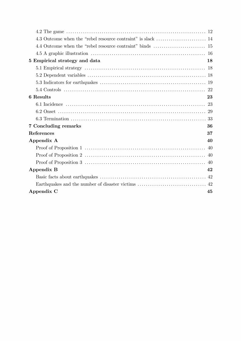
4.2 The game . . . . . . . . . . . . . . . . . . . . . . . . . . . . . . . . . . . . . . . . . . . . . . . . . . . . . . . . . . . . . . . . . . . 12

4.3 Outcome when the �rebel resource contraint�is slack . . . . . . . . . . . . . . . . . . . . . . . . 14

4.4 Outcome when the �rebel resource contraint�binds . . . . . . . . . . . . . . . . . . . . . . . . . 15

4.5 A graphic illustration . . . . . . . . . . . . . . . . . . . . . . . . . . . . . . . . . . . . . . . . . . . . . . . . . . . . . . . 16

5 Empirical strategy and data 185.1 Empirical strategy . . . . . . . . . . . . . . . . . . . . . . . . . . . . . . . . . . . . . . . . . . . . . . . . . . . . . . . . . . 18

5.2 Dependent variables . . . . . . . . . . . . . . . . . . . . . . . . . . . . . . . . . . . . . . . . . . . . . . . . . . . . . . . . . 18

5.3 Indicators for earthquakes . . . . . . . . . . . . . . . . . . . . . . . . . . . . . . . . . . . . . . . . . . . . . . . . . . . 19

5.4 Controls . . . . . . . . . . . . . . . . . . . . . . . . . . . . . . . . . . . . . . . . . . . . . . . . . . . . . . . . . . . . . . . . . . . . 22

6 Results 236.1 Incidence . . . . . . . . . . . . . . . . . . . . . . . . . . . . . . . . . . . . . . . . . . . . . . . . . . . . . . . . . . . . . . . . . . . 23

6.2 Onset . . . . . . . . . . . . . . . . . . . . . . . . . . . . . . . . . . . . . . . . . . . . . . . . . . . . . . . . . . . . . . . . . . . . . . . 29

6.3 Termination . . . . . . . . . . . . . . . . . . . . . . . . . . . . . . . . . . . . . . . . . . . . . . . . . . . . . . . . . . . . . . . . . 33

7 Concluding remarks 36References 37Appendix A 40Proof of Proposition 1 . . . . . . . . . . . . . . . . . . . . . . . . . . . . . . . . . . . . . . . . . . . . . . . . . . . . . . . . . . 40

Proof of Proposition 2 . . . . . . . . . . . . . . . . . . . . . . . . . . . . . . . . . . . . . . . . . . . . . . . . . . . . . . . . . . 40

Proof of Proposition 3 . . . . . . . . . . . . . . . . . . . . . . . . . . . . . . . . . . . . . . . . . . . . . . . . . . . . . . . . . . 40

Appendix B 42Basic facts about earthquakes . . . . . . . . . . . . . . . . . . . . . . . . . . . . . . . . . . . . . . . . . . . . . . . . . . . 42

Earthquakes and the number of disaster victims . . . . . . . . . . . . . . . . . . . . . . . . . . . . . . . . . 42

Appendix C 45

Acknowledgments

First of all, I wish to thank my supervisor, Ola Olsson, for all inspiring discussions

and for all ideas, feedback, and encouragement, without which this would not have been

possible. I have learned a lot from working together with you on two of the papers in this

thesis.

I am grateful to Arne Bigsten, Dick Durevall, Måns Söderbom, and everyone else in the

Development Economics Unit, for all discussions, suggestions, and insightful comments,

and to my two other coauthors, Gustav Hansson and David Yanagizawa, for all the fun

we had when we worked together on our papers.

My thanks also to all my fellow Ph.D. candidates and colleagues at the department

for their friendship, and for all the entertaining discussions we have had over the years,

and to the students and sta¤ at UC Berkeley, particularly Jørgen Juel Andersen, Niels

Johannesen, Gérard Roland, and Chad Jones, for making the semester I spent there so

stimulating and inspiring.

Many thanks to the administrative sta¤ at the department, particularly Eva-Lena

Neth Johansson and Jeanette Saldjoughi, for all practical assistance. I am grateful to

Dora Kós-Dienes, for assisting me in my application to UC Berkeley, and to Debbie

Axlid, for excellent editorial assistance.

Financial assistance from SIDA/Sarec and the Barbro Osher Pro Suecia Foundation

is gratefully acknowledged.

I wish to thank my wonderful family and my loyal friends for their love, friendship,

and support.

Finally, I want to thank Maria, the love of my life, for always being there, and for

giving my life joy and true meaning. I could not have done this without you.

Pelle Ahlerup

Bollebygd, Sweden, September 2009

ix

Summary of the thesis

The thesis consists of �ve self-contained papers.

Paper 1:Social Capital vs Institutions in the Growth Process

Is social capital a substitute or a complement to formal institutions for achieving

economic growth? Research on the impacts of social capital and formal institutions on

economic development have so far mainly emerged as two distinct �elds. In the social

capital literature, trust, networks, social norms, and associational activity are believed

to be central aspects of successful economies. Although micro studies suggest that social

capital has a larger e¤ect on economic performance when formal institutions are weak,

this has not been con�rmed at the macro level.

In the institutional literature, it is emphasized how formal institutions such as those

regulating the strength of property rights, the constraints against the executive, and the

power of courts, are fundamental determinants of long-run growth (North 1990, Acemoglu

et al. 2001). These studies, however, never attempt to quantify the e¤ect of informal

institutions such as interpersonal trust.

Based on the micro evidence, we outline an investment game between a producer

and a lender in an incomplete-contracts setting. The key insight from the model is that

social capital may have its greatest positive impact on the total monetary surplus from

the game (economic growth) at lower levels of institutional development, and that the

positive impact eventually vanishes if institutions become strong enough.

This basic prediction about substitution �nds support in a cross-country growth regres-

sion �the marginal impact of our proxy for social capital (interpersonal trust) decreases

with the quality of formal institutions. This implies that attempts at building social

capital create, if successful, a pro-growth potential for countries with bad institutions.

Paper 2:The Roots of Ethnic Diversity

The level of ethnic diversity is believed to have consequences for economic and political

development. Accepting this observation naturally leads to the question: Why are some

countries more ethnically fractionalized than others? For instance, why is the probability

that two randomly chosen individuals belong to di¤erent ethnic groups roughly 93 percent

in Uganda but only 0.2 percent in South Korea?

In the paper, we explore the two main hypotheses regarding the formation of ethnic

identities. The �constructivist�view is that ethnic identi�cations are socially constructed

phenomenon appearing during modernity (Gellner 1983, Tilly 1992). The �evolutionary�

view contends that ethnic divisions have deep roots in history and ecology and should

be analyzed in an evolutionary framework. Ethnic identi�cation is here regarded as a

x

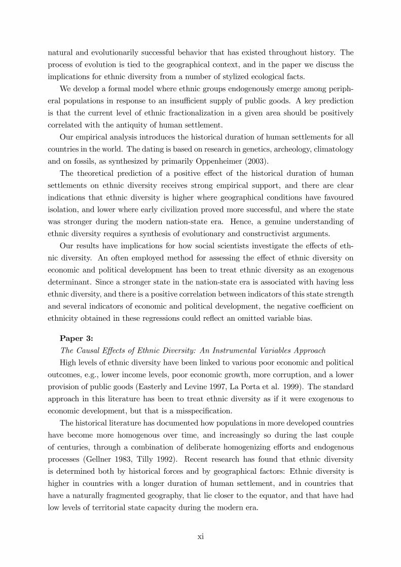
natural and evolutionarily successful behavior that has existed throughout history. The

process of evolution is tied to the geographical context, and in the paper we discuss the

implications for ethnic diversity from a number of stylized ecological facts.

We develop a formal model where ethnic groups endogenously emerge among periph-

eral populations in response to an insu¢ cient supply of public goods. A key prediction

is that the current level of ethnic fractionalization in a given area should be positively

correlated with the antiquity of human settlement.

Our empirical analysis introduces the historical duration of human settlements for all

countries in the world. The dating is based on research in genetics, archeology, climatology

and on fossils, as synthesized by primarily Oppenheimer (2003).

The theoretical prediction of a positive e¤ect of the historical duration of human

settlements on ethnic diversity receives strong empirical support, and there are clear

indications that ethnic diversity is higher where geographical conditions have favoured

isolation, and lower where early civilization proved more successful, and where the state

was stronger during the modern nation-state era. Hence, a genuine understanding of

ethnic diversity requires a synthesis of evolutionary and constructivist arguments.

Our results have implications for how social scientists investigate the e¤ects of eth-

nic diversity. An often employed method for assessing the e¤ect of ethnic diversity on

economic and political development has been to treat ethnic diversity as an exogenous

determinant. Since a stronger state in the nation-state era is associated with having less

ethnic diversity, and there is a positive correlation between indicators of this state strength

and several indicators of economic and political development, the negative coe¢ cient on

ethnicity obtained in these regressions could re�ect an omitted variable bias.

Paper 3:The Causal E¤ects of Ethnic Diversity: An Instrumental Variables Approach

High levels of ethnic diversity have been linked to various poor economic and political

outcomes, e.g., lower income levels, poor economic growth, more corruption, and a lower

provision of public goods (Easterly and Levine 1997, La Porta et al. 1999). The standard

approach in this literature has been to treat ethnic diversity as if it were exogenous to

economic development, but that is a misspeci�cation.

The historical literature has documented how populations in more developed countries

have become more homogenous over time, and increasingly so during the last couple

of centuries, through a combination of deliberate homogenizing e¤orts and endogenous

processes (Gellner 1983, Tilly 1992). Recent research has found that ethnic diversity

is determined both by historical forces and by geographical factors: Ethnic diversity is

higher in countries with a longer duration of human settlement, and in countries that

have a naturally fragmented geography, that lie closer to the equator, and that have had

low levels of territorial state capacity during the modern era.

xi

In the paper we discuss how previous studies on ethnic diversity and long-run devel-

opment may have obtained biased estimates due to omitted variables, simultaneity, or

measurement error, but also that the use of instrumental variables allows us to deal with

exactly these problems.

Our main instruments capture the historical duration of human settlements, the degree

of geographical fragmentation, and the number of years since the date of independence.

With these at hand, we �nd that high levels ethnic diversity is associated with lower

income levels, poor economic growth, more corruption, and poor provision of public goods,

and that results obtained in OLS may underestimate the true e¤ects. While previous

studies have shown signi�cant partial correlations between ethnic diversity and economic

outcomes, the present paper demonstrates that there indeed are causal e¤ects of ethnic

diversity.

We also �nd that the e¤ects of ethnic diversity and property rights institutions on

economic development among former European colonies can be separated from each other.

This suggests that countries that have problems due to high levels of ethnic diversity

could alleviate these problems by improving the quality of their formal institutions. On a

more general level, the results presented in the paper promise that an acceptance of the

endogenous nature of ethnic diversity does not preclude meaningful empirical analyses of

the long-run e¤ects of ethnic diversity.

Paper 4:Nationalism and Government E¤ectiveness

Nation-building, which generally refers to a process of unifying the population in a

country by constructing a national unity, is believed to have positive e¤ects on aggregate

performance, and has been proposed as a possible remedy against problems associated

with high levels of ethnic fractionalization (Miguel 2004). However, systematic empirical

evidence that the creation of a national unity is a worthwhile policy is still largely absent,

and nationalism, an indicator of successful nation-building, has been empirically linked

to protectionism and intolerance, which suggests that dismal performance is a more likely

outcome. Furthermore, there is an obvious problem with the idea that the unity of a

country�s population can be enhanced by encouraging nationalism �a national identity

is created in relation to other national identities, and for there to be an �us�there has to

be a �them.�

The paper investigates whether nationalism a¤ects the ability of governments to e¤ec-

tively formulate and implement good policies, i.e., government e¤ectiveness, and whether

it mitigates the negative e¤ects of ethnic fractionalization, or is associated with less trade

openness. We discuss how nationalism may have a positive e¤ects, as it can increase in-

group altruism, trustworthiness, and state authority, and how it may have negative e¤ects,

as it can breed prejudice, out-group animosity, and skepticism of new ideas, implementa-

xii

tion techniques, and goods, if these are not of national origin or are not considered to be

in line with national traditions. We hypothesize that the positive e¤ects will dominate

at low levels of nationalism but that the negative e¤ects will dominate at higher levels of

nationalism.

The empirical analysis con�rms that nationalism has an inverted U-shaped e¤ect on

government e¤ectiveness, and also shows that this e¤ect does not capture the in�uence

of factors such as income, economic growth, democracy, and income inequality. Comfort-

ingly, the qualitative result is the same also when we instrument for nationalism, with

instruments that represent a number of historical and cultural circumstances. Further-

more, nationalism can mitigate the negative e¤ects of ethnic fractionalization in former

colonies, but has no clear e¤ect on trade openness.

Taken seriously, the results suggest that most countries already have too nationalistic

populations, and probably would function better if these sentiments where downplayed.

Paper 5:Earthquakes and Civil War

There are two diametrically opposing views in the literature on natural disasters and

violent con�ict. According to the �rst view, natural disasters can contribute to de-escalate

con�ict, as previous disagreements seem relatively unimportant. This is view shared by

several relief organizations and policy makers (WBGU 2008, Brancati 2007).

The second view is that natural disasters make violent con�ict more likely, and this

view is supported by most systematic empirical studies. Nel and Righarts (2008) �nd that

natural disasters in general increase the probability of onset of civil war, and Brancati

(2007) �nds that earthquakes are positively associated with the incidence of civil war, and

argues that earthquakes of higher magnitude have a stronger e¤ect.

Consider the e¤ects of the great tsunami in South-East Asia in 2004. The tsunami is

believed to have exacerbated the con�ict in Sri Lanka, but in Aceh, Indonesia, the �ghting

came to an end. It appears that the con�ict de-escalated where the tsunami had its most

severe e¤ects and escalated where the e¤ects were less severe.

In the paper we ask whether more destructive natural disasters are associated with a

higher or a lower risk of violent con�ict. We take the argument that natural disasters can

de-escalate existing con�icts seriously, and investigate the e¤ects not only on the incidence

or onset of con�ict, but also on the termination of con�ict.

We develop an economic model of rebellion in the wake of a natural disaster. It

shows how the moderate destruction caused by moderate natural disasters can make

rebellion feasible, by lowering the opportunity cost of potential recruits. More intensive

destruction means that the material payo¤ in the event of a victorious rebellion is lower.

Taken together, the model predicts that violent con�ict may be more likely after moderate

disasters and less likely after very strong disasters.

xiii

The empirical results are well in line with the theoretical predictions. We employ an

exhaustive dataset on earthquakes from 1947 to 2001, and develop a new set of exogenous

indicators of the size of earthquakes, e.g., the seismic energy released by earthquakes. We

�nd that earthquakes a¤ect both the onset and termination of con�icts and, as a result,

the incidence of con�ict. The size of an earthquake is of fundamental importance, as are

the social conditions in the area surrounding the epicenter.

The association between earthquakes and the incidence of civil war can be explained

by three e¤ects: (i) Moderate earthquakes increase the risk that new con�icts are started,

(ii) strong earthquakes make it less likely that new con�icts are started, and (iii) strong

earthquakes make the termination of existing con�icts more likely. As such, the paper is

the �rst systematic study to establish that a natural disaster can give the impetus needed

to end existing con�icts and prevent new violent con�icts from emerging.

ReferencesAcemoglu, D., S. Johnson, and J. Robinson (2001) �The Colonial Origins of Comparative

Development. An Empirical Investigation�American Economic Review, 91(5):1369-401.

Alesina, A. and E. La Ferrara (2005) �Ethnic Diversity and Economic Performance�Journalof Economic Literature, 43(3):762-800.

Brancati, D. (2007) �Political Aftershocks: The Impact of Earthquakes on Intrastate Con-�ict�Journal of Con�ict Resolution, 51(5):715-43.

Easterly, W. and R. Levine (1997) �Africa�s Growth Tragedy: Policies and Ethnic Divisions�Quarterly Journal of Economics, 112(4):1203-50.

Gellner, E. (1983) Nations and Nationalism, Oxford: Blackwell.

La Porta, R., F. Lopez-de-Silanes, A. Schleifer, and R. Vishny (1999) �The Quality ofGovernment�Journal of Law, Economics & Organization, 15(1):222-79.

Mauro, P. (1995) �Corruption and Growth�Quarterly Journal of Economics, 110(3):681-712.

Miguel, E. (2004) �Tribe or Nation? Nation-building and Public Goods in Kenya versusTanzania�World Politics, 56:327-62.

Nel, P. and M. Righarts (2008) �Natural Disasters and the Risk of Violent Civil Con�ict�International Studies Quarterly, 52(1):159-85.

North, D. (1990) Institutions, Institutional Change, and Economic Performance, Cambridge:Cambridge University Press.

Oppenheimer, S. (2003) Out of Eden: The peopling of the World, London: Constable.

Tilly, C. (1992) Coercion, Capital, and European States, AD 990-1992, Oxford: Blackwell.

WBGU (2008) Climate Change as a Security Risk, available online at http://www.wbgu.de/wbgu_jg2007_engl.html.

xiv

European Journal of Political Economy 25 (2009) 1–14

Contents lists available at ScienceDirect

European Journal of Political Economy

j ourna l homepage: www.e lsev ie r.com/ locate /e jpe

Social capital vs institutions in the growth process

Pelle Ahlerup a,⁎, Ola Olsson a, David Yanagizawa b

a Department of Economics, University of Gothenburg, Box 640, 40530 Göteborg, Swedenb Institute for International Economic Studies, Stockholm University, 10691 Stockholm, Sweden

a r t i c l e i n f o

⁎ Corresponding author. Tel.: +46 31 786 1370; fax:E-mail address: [email protected] (P.

0176-2680/$ – see front matter © 2008 Elsevier B.V. Adoi:10.1016/j.ejpoleco.2008.09.008

a b s t r a c t

Article history:Received 25 March 2008Revised 22 September 2008Accepted 23 September 2008Available online 4 October 2008

Is social capital a substitute or a complement to formal institutions for achieving economicgrowth? A number of recent micro studies suggest that interpersonal trust has its greatestimpact on economic performancewhen court institutions are relatively weak. The conventionalwisdom from most macro studies, however, is that social capital is unconditionally good forgrowth. On the basis of themicro evidence, we outline an investment game between a producerand a lender in an incomplete-contracts setting. A key insight is that social capital will have thegreatest effect on the total surplus from the game at lower levels of institutional strength andthat the effect of social capital vanishes when institutions are very strong. When we bring thisprediction to an empirical cross-country growth regression, it is shown that the marginal effectof social capital (in the form of interpersonal trust) decreases with institutional strength. Ourresults imply that a one standard deviation rise in social capital in weakly institutionalizedNigeria should increase economic growth by 1.8 percentage points, whereas the same increasein social capital only increases growth by 0.3 percentage points in strongly institutionalizedCanada.

© 2008 Elsevier B.V. All rights reserved.

JEL classification:O17O43O57

Keywords:Social capitalInstitutionsEconomic growthInvestment

1. Introduction

Research on the impacts of social capital and formal institutions on economic development have so far mainly emerged as twodistinct fields. In the former literature, trust, networks, social norms, and associational activity are believed to be central aspects ofsuccessful economies. In the institutional literature, formal rules of the game such as property rights laws and the strength ofcourts are regarded as critical for development. We argue that there is an important disconnection between results from microstudies of social capital – which indicate that various self enforcement mechanisms are more prevalent when contractinginstitutions are weak – and macro studies where social capital-related measures are hypothesized to have a uniform positiveimpact on economic performance.

In this article, we outline a unified theoretical framework of the relative importance of social capital and formal institutions in asimple principal-agent investment model featuring a producer and a lender in an incomplete contract-setting. The probability ofcontract enforcement by an exogenous court is our major indicator of institutional strength and social capital enters our model asan extra ‘social’ or ‘intrinsic’ payoff to both players from acting trusting or trustworthy. The major insight from our model is thatsocial capital tends to have its greatest positive impact on the total monetary surplus from the game (economic growth) at lowerlevels of institutional development and that the positive impact eventually vanishes if institutions become strong enough.

This basic prediction about substitution is then brought to the macro level and tested in a cross-country growth regression. Inaccordance with our hypothesis, our results show that the marginal impact of our proxy for social capital (interpersonal trust)decreases with the quality of formal institutions. More precisely, our results imply that a one standard deviation increase in social

+46 31 786 1326.Ahlerup).

ll rights reserved.

mailto:[email protected]

http://dx.doi.org/10.1016/j.ejpoleco.2008.09.008

http://www.sciencedirect.com/science/journal/01762680

2 P. Ahlerup et al. / European Journal of Political Economy 25 (2009) 1–14

capital leads to a 1.10 percentage points increase in the growth rate among countries at the 25th percentile of institutional strength,whereas the effect among countries at the 75th percentile of institutional strength is only 0.36 percentage points. Our results arerobust to using an instrumental variables-methodology where we take into account that social capital and institutions might beendogenous to growth or indeed have a causal impact on each other.

Our approach combines two major types of building blocks: (1) The literature on the macroeconomic effects of formalinstitutions and (2) the extensive empirical literature on the micro and macro effects of social capital. Starting with institutionaleconomics, this tradition emphasizes how formal institutions such as those regulating the strength of property rights, theconstraints against the executive, and the power of courts are fundamental determinants of long-run growth. Following in thefootsteps of North (1981, 1990), a number of seminal contributions have emerged over the recent decade such as Knack and Keefer(1995), Hall and Jones (1999), Acemoglu et al. (2001, 2002), Acemoglu and Johnson (2005), and Banerjee and Iyer (2005). Thesestudies all show that good formal institutions are strongly associatedwith prosperity, although joint endogeneity problems are stillan important econometric issue in the literature. Unlike our study, this literature also aims at explaining why some countries havebetter formal institutions than others. None of these studies, however, attempt to quantify the effect of informal institutions suchas social networks or interpersonal trust. Acemoglu and Johnson (2005) differentiate between court (‘contracting’) and propertyrights institutions, but do not study the impact of private enforcement mechanisms.

Social capital is arguably one of the most elusive concepts in social science. As discussed by Bjornskov (2006), there are at leastthree important dimensions of social capital: generalized trust, social norms, and associational/network activity. In this paper, wewill focus on social capital as generalized trust among people, i.e. an optimistic expectation about the behavior of fellow citizens,many of whom we do not know personally. The empirical cross-country macro literature on social trust includes seminalcontributions by Knack and Keefer (1997) and Zak and Knack (2001).1 The paper most closely related to ours is Zak and Knack(2001) who regress economic growth on both levels of interpersonal trust (from World Value Surveys, WVS) and on an index offormal institutional strength in a cross-section of 41 countries, most of which are industrialized. The authors find thatinterpersonal trust is positively and significantly related to growth when holding formal institutions constant. However, they donot explore the possibility of non-linear effects of trust that depend on different levels of formal institutions. In a robustnessanalysis of Zak and Knack (2001), Beugelsdijk et al. (2004) find that the results are in general fairly robust, even when includingsome institutions-related measures (such as religion and political instability), but that the marginal impact of trust is greater inlow-trust countries. Similarly, Tabellini (2006) finds a positive effect of interpersonal trust on growth in European regions using aninstrumental variable approach, but does not analyze any differential effects depending on formal institutions.2

The overall picture in the micro studies is mixed but nevertheless suggests that social capital has a larger effect on economicperformance when formal institutions areweak. Table 1 shows a summary of some of the more well-known studies.3 For instance,Bigsten et al. (2000) and Fafchamps and Minten (2002) both confirm that social capital has a strong role when property rights andcourts areworking imperfectly. Themain hypothesis that emerges from thesemicro studies is therefore that social trust and formalinstitutions should be primarily substitutes in the growth process at the macro level.

Our paper is not the first effort that tries to understand howmicro results on trust can be translated to amacro level. Beugelsdijk(2006) argues that it is conceptually difficult to move from micro results to a macro level when it comes to social capital and thatgeneralized trust as measured by the WVS might actually capture the quality of formal institutions, a claim that Uslaner (2008)strongly refutes.4 In a similar vein, Bjornskov's (2006) empirical analysis suggests that social trust has a positive impact on thequality of government, whereas Rothstein (2000) argues that it is rather good government that causes general trust. Our analysisdeparts from these studies by treating social trust and institutions as two distinct factors and by estimating whether they aresubstitutes in development, as our model predicts. Furthermore, our use of instrumental variables arguably neutralizes theconcerns referred to above about the possible linkages between generalized trust and formal institutions.

In summary, we argue that our article offers two specific contributions to the literature. Firstly, our simple modellingframework rationalizes the empirical regularity from the micro level that social capital affects growth and investment mainlywhen institutions are relatively weak. Secondly, our article is the first one to demonstrate empirically (and with the use of IV-methods) that generalized trust and institutional quality are substitutes for growth.

The article is organized as follows. In Section 2we present themodel and derive the key results for the relevance of social capitaland institutions. In Section 3 we display the empirical specifications and present the results. Section 4 concludes the exposition.

2. The model

In order to provide an aid for thinking about the effects of institutions and social capital on growth, we present in this section asimple model of an investment game between a Lender and a Producer, inspired by the empirical literature referred to above. Thepurpose of the model is to provide a micro-foundation for our hypotheses regarding the interrelationships between social capitaland institutions at the macro level.

1 See Durlauf (2002) and Durlauf and Fafchamps (2005) for a critical discussion of this line of research.2 Tabellini uses data from 69 regions in 8 Western European countries and includes country fixed effects. The instruments used are literacy rate around 1880

and constraints on the executive in the years 1600–1850. However, he does not include any measures of formal institutions at the regional level. Studying datafrom 54 European regions, Beugelsdijk and van Schaik (2005) find that associational activity is the best predictor or growth.

3 The results referred to in the table should not be thought of as having a perfect correspondence with each other or with our model since the mentionedstudies all use different methodologies. We believe they still well illustrate our basic point.

4 See also Beugelsdijk's recent reply to Uslaner (Beugelsdijk, 2008).

Table 1Relevant studies on social capital and institutions

Author(s) Agents Social Capital measure(s) Institutional measure(s) Relevant Findings

Beckmann andRoger (2004)

Hog farmers inPoland

Dependence on buyer;duration of business relationship;buyer specific investments

Farmers' perceptions ofcourt strength

Farmers are unwilling to takecases to court when the measuresof social capital are high

Beugelsdijk andSmulders (2004)

Citizens of 54Europeanregions

Density of associational activity;importance of family and friends.

None Bridging social capital(associational activity) is positivelyrelated to economic growth whereasbonding social capital (family ties, etc)is not.

Bigsten et al. (2000) Manufacturing firmsin 6 African countries

Length of business relationship. None Renegotiations of broken contracts arehelped by (trust creating) long-termrelations. Better institutions mayencourage risk taking and thereforealso lead to more recourse to courtsin case of contract breach.

Fafchamps andMinten (2002)

Agriculturaltraders inMadagascar

Number of relatives in agriculturaltrade; traders known; and potentialinformal lenders

None Positive effect on firm productivity forbetter connected traders. Social capitallowers transaction costs.

Grootaert andNarayan (2004)

Households in 4rural communitiesin Bolivia.

Membership in local associations. “Effectiveness anduniversality ofmunicipal government”

Social capital matters more for the poorthan the non-poor. Social capital has apositive effect on welfare only in themore weakly institutionalizedcommunities.

Guiso, Sapienza andZingales (2004)

Households inItaly

Electoral turnout, blooddonation and trust (as measuredby World Value Surveys).

Mean number of years ittakes to complete afirst-degree trial.

More social capital implies a morefrequent use of checks, more investmentin stocks as apposed to cash and moreinstitutional rather than informal credit.The effect is stronger in areas with weakerlegal enforcement.

Johnson, McMillanand Woodruff (2002)

Firms andcustomers in 5East Europeancountries

Relational contracting Stated belief that courtscan enforce contracts.

Trust-based interaction(“relational contracting”) more likely wheninstitutions are weak.

Krishna (2001) Villages in ruralIndia.

An index of labour-groupparticipation, assessments on thecooperative attitude, and trust,solidarity and reciprocity.

Various variables measuringthe agency power: howstrong are the caste leaders;local government;patron–client links;political parties' power;village councils and thecapacity of young andeducated leaders.

Social capital is beneficial for developmentonly if it is activated by agency power (i.e.needs some minimum level of institutions).Social capital without agency power doesnot help development.

McMillan andWoodruff (1999)

Managers ofmanufacturingfirms in Vietnam

Percent of relationships involvingcommunity sanctions and networks

None Social capital is important since courts andprivate property rights are weak. Loss offuture business opportunity is not animportant sanction. Instead, scrutinizationof potential clients, community sanctions,and renegotiation are commonly used.

Miguel, Gertler andLevine (2005)

Districts inIndonesia

Relative expenditures on festivalsand ceremonies and a subjectiveassessment on the traditional levelof ethic and mutual cooperation.A number of measures of formalcommunity groups.

None Initial level of social capital does not predictsubsequent industrial development.

3P. Ahlerup et al. / European Journal of Political Economy 25 (2009) 1–14

Themodel is a sequential, principal-agent investment gamewith a representative Lender and Producer and a Court as describedin extensive form in Fig. 1.5 We have chosen to analyze an investment problem since it is standard to regard investment as a keyengine of economic growth, but similar types of situations also apply in supplier-producer and buyer-seller situations with tradecredit. We also believe that this type of game is quite similar to the scenarios described in the empirical literature referred to above.The game is one of perfect information and players are assumed to be risk neutral and non-cooperative. There are no other agentsin the economy.

In the initial Credit Stage, Lender chooses whether to lend the required amount of capital k or not. If she chooses not to, thegame ends, no production occurs, and payoffs are uL=uP=0 for Lender and Producer respectively. This is the ‘autarkic’ or status quosituation where agents remain in subsistence production.

5 A similar but more complex model of “trust in the shadow of the court” is provided by Brennan et al. (2003).

Fig. 1. The investment game.


In the second Contract Stage, the players have entered a market economy where a lending of k units of capital has occurred andproduction has been undertaken. Producer considers the option of fulfilling the credit contract which would result in Producerreceiving a net monetary payoff of πPN0 plus a non-monetary social benefit of cooperation sPN0, discussed further below.Likewise, Lender would in this case be repaid the credit amount k and in addition get a monetary compensation πLN0 and a socialpayoff from being trusting sLN0. This is also the socially optimal situation in the sense that it maximizes aggregatewelfare and totalmonetary payoffs.

The si-terms capture rewards stemming from the trust and trustworthiness among our representative agents. The players mayor may not have a previous history of interactions and the trust they show should be regarded as generalized trust and notnetwork-specific. These extra payoffs are a kind of social reward such as a strengthened reputation or the moral satisfaction fromliving up to the positive expectation of cooperation.6 The payoffs only materialize if the player in question has shown a trusting andcooperative behavior in the first and second states. If Producer reneges in the second stage, he forgoes this social payoff whereasLender retains it throughout the game if she has provided the credit in the first stage and thereby proved to be a trusting person.We further assume that social payoffs are fully observable by both players.

The conventional payoffs from the investment πP and πL have been agreed upon in the contract. πL could take the form of aninterest payment to Lender or indeed as profit-sharing of some form.We leave it open herewhat type of financing arrangement thetwo players have agreed upon, although we could have easily made such a choice endogenous.

The other option for Producer is to renege on the contract, by which is meant that he retains the compensation to Lender πL thatwas stipulated by the contract and repudiates Lender's claims to a repayment of k. The dispute may then end up in court in thethird stage. This is the Lawsuit Stage, where the Lender decides whether to take the reneging Producer to court or not.7 Should the

6 See for instance Brennan et al. (2003), Guth and Ockenfels (2005) and Francois and Zabojnik (2005) for similar ‘intrinsic rewards’ from cooperation.7 Historically, the existence of state-supported courts have certainly not always been in place or been strong enough to be a relevant alternative for agents

involved in a contract dispute. Greif (1993, 2006) documents how merchant guilds and coalitions of traders in Medieval times often proved to be more efficientinstitutions for solving contract issues than institutions provided by the state.


Lender choose not to go to court the Producer keeps the total monetary payoff from the project πL+πP while we assume that hecannot benefit from the credit k that he has failed to repay.8 The Lender is left with a social payoff sL and with a loss of his credit.9 IfLender chooses to go to court, the court will enforce the contract with a probability β, which is our indicator of the strength ofcontracting institutions. β is simply meant to reflect how strong courts are and is not intended to imply any form of strategicinteraction between the Court and the Producer. The cost of going to court is covered by a loser-pays-principle, according to whichthe losing party pays a fine of d to the court. If the contract is properly enforced, Lender gets her credit in return and receives a netpayoff of πL+sL while Producer receives πP−d.

If the contract is not enforced by the court, Producer ends upwith πL+πP. Lender receives no compensation and no repayment ofthe credit and thus receives a net utility of −k−d+sL from lending. Obviously, many Lenders would require some form of collateralfor the loan, but for simplicity we abstract from that in this simple setting. We also leave out aspects like the degree of contractcomplexity or additional social costs of a negative court ruling.

Using the payoff structure above, we can easily derive the following set of solutions.

Solutions. The best response strategies of the players and the SPNE of the game are determined by the following conditions:

L

8 Weassump

9 Anoreturn f10 Seetrust ap

Credit stage Lenderð Þ:f Lend if any of the following conditions applies :ið Þ LusL + β πL + k + dð Þ− k − d � 0

iið Þ sL − k � 0iiið Þ Producer will fulfill

Not lend if noneof ið Þ; iið Þ;or iiið Þ applies:

Contract stage Producerð Þ: f Fulfill if FusP + β πL + dð Þ− πL � 0Renegeotherwise

awsuit stage Lenderð Þ: fNot to Court if sL − k � 0 andβ πL + k + dð Þ− d � 0ToCourt otherwise:

e key expressions above are L=L(sL,β,πL,k,d) and F=F(sP,β,πL,d) which determine whether the socially optimal equilibrium
Th(Lend, Fulfill) is obtained or not. Lender's willingness to lend and Producer's willingness to fulfill will increase with the socialpayoffs from trustworthy behavior sL and sP and from the strength of court institutions β. Social capital and institutions aresubstitutes in the sense that either increases in sL and sP or an increase in β could make L or F positive. The size of the investment,given by k, affects Lender in the sense that she becomes more cautious and less willing to lend as k increases. The Lender'swillingness to lend will be positively associated with her investment returns πL , whereas these will have a negative influence onProducer's willingness to fulfill since a higher level makes it more tempting to try to appropriate this payoff.
Disregarding all other variables for a moment and assuming that sL=sP=sbk, we can write L(s,β) and F(s,β). Let us imagine asituation where court institutions are at a low level βlow such that L(s,βlow)b0 and F(s,βlow)b0, which means that monetarypayoffs are (0, 0). There is then a ΔsN0 such that either L(s+Δs,βlow)=0 or F(s+Δs,βlow)=0, which means that Lender supplies thecredit and production occurs. In other words, at low levels of β, an increase in social capital s can lead to economic development.However, at a high level of court strength βhigh such that L(s,βhigh)≥0 and F(s,βhigh)≥0 , the socially optimal equilibrium is alreadyobtained and an equivalent increase Δswill have no effect. Hence, social capital increases will have a stronger positive effect wheninstitutions are weak.

As was mentioned in the introduction, we do not attempt to explain how court institutions and social capital have emerged inthe first place, but we recognize that they could both be driven by the same underlying set of forces (history, geography, ethnicfractionalization, etc.) and are likely to be positively correlated.10 Let us think of s as being proportional to the average level of socialcapital in society, i.e. the total stock of interpersonal trust that has accumulated over the years. We assume that the higher theaverage level, the greater the payoff from acting trustworthy. Equivalently, if the average level of trust is small, people will not beexpected to cooperate and the social opportunity cost of reneging (s) should be relatively small.

make this assumption so that a failure to act trustworthy is also associated with a kind of waste in terms of total monetary payoffs. This is not a criticaltion but simplifies derivations.ther possibility, often observed in reality, is that Lender offers a renegotiation at this point, offering Producer not to be socially disgraced, perhaps inor the credit and a smaller part of the net surplus from the investment.for instance Congdon Fors and Olsson (2007) for a model of endogenous institutional change and Bjornskov (2006) for an empirical analysis of how socialpears to cause good governance.

Fig. 2. Investment game equilibria under varying strengths of court institutions and social capital. Note: The figure is based on the results in Solutions, assuming thefollowing parameter values: πL=πP=3, k=2, d=1, sL=sP=s.


As a further illustration of the model, we provide a numerical example in Fig. 2 where we assume πL=πP=3, k=2, d=1, sL=sP=s .The example assumes a relatively small investment with a relatively high total payoff and a payoff/investment ratio of (πL+πP)/k=6/2=3. The simplification allows us to analyze the relationship between the two remaining variables in the system; the strengthof court institutions β and the social payoff s. The potential outcomes of this game follow from Solutions above. The A-area showsthe ‘input requirement set’ of court strength and social capital for the (Lend, Fulfill)-equilibrium to apply. The line defined byβ = 3 − s

4 shows the combinations of β and swhere Producer is indifferent about reneging or fulfilling. The curve is negatively slopedand linear, indicating that in this setup social capital and formal institutions are perfect substitutes. The equivalent line for Lenderis given by β = 3 − s

6 in the s∈ [0,2)-interval. In the B-area are the combinations where the players end up in court. The area definedby β � 1

6 and s≥2 makes up the C-area where Producer reneges but Lender will not go to court. Since β and s in reality tend to becorrelated, it is rather unlikely that an economy could end up here. The D-area, lastly, hosts combinations where βb 3 − s

6 and sb2,which yields the outcome with no investment (0,0).

The main point of the figure is to illustrate intuitively how the effect of an exogenous increase in social capital can depend onthe level of institutional strength. The four arrows in the A, B, and D-areas show equally large increases in social capital.11 In the A-area, an increase in s has no effect since the players are already in the good equilibrium. This might be thought of as equivalent to afirst-best outcome which would always be in place if institutions were perfect. Two arrows originate in the D-area. The lowerplaced arrow shows that higher social capital may not be enough to push the economy into a better equilibrium. As mentionedabove, we do not think that this scenario with a very low β and a relatively high s is often observed in reality.12 The upper arroworiginating in the D-area shows that beginning at a higher level of court strength canmake all the difference. In the B-area, finally –

where Lender supplies the credit, Producer reneges, and the contract is settled in court – an increase in social capital is very likelyto lead to the good equilibrium.

In summary, the simple framework employed here gives at least three insights. First, our model has the feature that formalinstitutions and social capital can be substitutes in the pursuit of the growth-maximizing equilibrium. Second, the model showsthat at high levels of institutional strength, social capital can be irrelevant for the ‘growth outcome’. Thirdly, at low andintermediate levels of institutional strength, increases in social capital might have a positive effect on the total payoff frominvestment. The model thus implies that the impact of an increase in social capital should decrease with the level of institutionalstrength.

3. Empirical evidence

Our model and overview of the micro literature indicate that the effect of social capital on economic performance is nonlinearand will depend on the quality of institutions. Likewise, the effect of institutions on economic performance will differ betweenlow-trust countries and high-trust countries. To keep our investigation comparable to the focal papers in the literature on socialcapital and growth, Knack and Keefer (1997) and Zak and Knack (2001), we employ a standard cross-country Barro-style growthmodel. Besides comparability with previous research this has two additional advantages—we can use what may be the best proxy

11 We recognize that the effect of exogenous increases in institutional strength also will depend on the level of social capital.12 Such a scenario might perhaps be observed in countries where the state has more or less collapsed and where social bonding has taken its place, as in Somaliain the 1990s. Such countries will, however, not be included in our empirical analysis.

Table 2Variable descriptions

Variable Name Variable description Source

Main variablesGrowth Annual growth in GDP per capita1995–2005 World Bank (2006a)InitInc Log GDP per capita (Constant Prices: Laspeyres) Heston et al. (2006)InvPrice Price level of investment, PPP Heston et al. (2006)LifeExp Life expectancy at birth, total (years) World Bank (2006a)Trust [ = Trust (v.1)] Interpersonal trust in survey 1990–95 (+96, 97, 81–89 if missing) WVS (2006)Inst. Quality of government, ICRG Teorell et al. (2006)

Other variablesbri_col British colony CEPII (2006)Bureaucratic delays 1972–1995 Bureaucratic delays 1972–1995, BERI Teorell et al. (2006)Composite contract enforcement Composite court quality, calculated as the mean of

the other three measures from World Bank (2006b)World Bank (2006b)

Contract enforceability 1982–89 Contract enforceability, 1982–89, BERI La Porta et al. (1997)Cost of contract enforcement Cost to enforce contract (norm) in 2003 World Bank (2006b)Days for contract enforcement Time to enforce contract (norm) in 2003 World Bank (2006b)Abslat Absolute latitude in degrees CEPII (2006)Distcr Mean distance to coast or river CID (2001)esp_col Spanish colony CEPII (2006)Ethnic fractionalization Ethnic fractionalization Alesina et al. (2003)Ethnic polarization (mean) ETH12POL Reynal-Querol (2006)fra_col French colony CEPII (2006)InvRate Gross capital formation in 2000 (% of GDP) World Bank (2006a)legor_fr French legal origin La Porta et al. (1997)legor_sc Scandinavian legal origin La Porta et al. (1997)legor_so Socialist legal origin La Porta et al. (1997)legor_uk British legal origin La Porta et al. (1997)Linguistic fractionalization Linguistic fractionalization Alesina et al. (2003)Procedures in contract enforcement Procedures to enforce contract (norm) in 2003 World Bank (2006b)prt_col Portuguese colony CEPII (2006)Relative InvPrice PI/P, where P=Price Level of Gross Domestic Product and PI= PPP

over investment/XRAT in Current PricesHeston et al. (2006)

Quality of public institutions, 1982 Quality of public institutions, 1982 Teorell et al. (2006)Religious fractionalization Religious fract. Alesina et al. (2003)Religious polarization Rel pol Reynal-Querol (2006)Risk of expropriation 1982–1997 Risk of expropriation 1982–1997, ICRG Glaeser et al. (2004)State antiquity State antiquity by 1950, v3. Putterman (2006)Trade (Exports+Imports) /GDP World Bank (2006a)Trust (v.2) Interpersonal trust in survey 1990–95 (+96–99, 81–89 if missing) WVS (2006)Trust (v.3) Interpersonal trust in survey 1981–95 WVS (2006)Trust (v.4) Interpersonal trust in survey 1990–95 WVS (2006)Trust (v.5) Interpersonal trust in survey 1981–2004 WVS (2006)


available for social capital, interpersonal trust from World Values Surveys (WVS), and yet have sufficient variation in institutionalquality. The growth regression technique has well-known drawbacks (see e.g. Brock and Durlauf, 2001; Durlauf, 2002) but it canreveal interesting patterns of correlation and the results are straightforward to interpret. To the standard package of regressors,initial income, investment, and human capital, we add social capital and institutions.

Table 3Descriptive statistics for main variables

Variable N Mean SD Min Max

For countries and variables in specification (4.5)Growth 46 2.42 1.44 −0.36 7.87InitInc 46 9.23 0.85 6.85 10.29InvPrice 46 86.91 30.65 33.85 171.16LifeExp 46 72.05 6.86 45.18 79.54Trust 46 0.32 0.16 0.05 0.66Inst 46 0.76 0.21 0.36 1.00

For countries and variables in specification (5.5)InvRate 61 22.31 3.93 13.69 32.76InitInc 61 9.28 0.85 6.98 10.78InvPrice 61 67.06 23.47 17.63 137.50LifeExp 61 72.89 6.89 43.78 81.08Trust 61 0.30 0.14 0.05 0.66Inst 61 0.68 0.21 0.31 1.00


3.1. Model and data

The econometric models we employ will be variations on

13 All14 Bycountrinationashort, thon dom15 Zakcausalitin 19961997, anVenezu16 Insteven mcorrelatconcern17 Zaktheir esours.

ið Þ growthi;1995�2005iið Þ investment ratei;2000

� �= β0 + β1dinitial incomei + β2dinvestment pricesi + β3dhuman capitali + β4dsocial capitali

+ β5dinstitutionsi + β6dsocial capitalidinstitutionsi + errori:

r predictions are that β4, β5N0 but β6b0. Where possible we will use initial values as regressors to mitigate concerns of
Oureversed causality.13 In our main regressions we use growth in real per capita GDP and life expectancy from the World Bank(2006a) and initial income and investment prices from Heston et al. (2006).14 Interpersonal trust is coded from WVS data as theweighted share of respondents answering that “most people can be trusted”when asked “Generally speaking, would you say thatmost people can be trusted, or that you can't be too careful in dealing with people?”.
Interpersonal trust as it appears in WVS is an imperfect measure for social capital, as discussed by for instance Beugelsdijk(2006). In our model we pick one aspect whereby social capital can affect economic performance— that individuals gain a positiveutility from being trusting and acting honestly. When more people are honest and trusting, we will see a larger fraction of therespondents answering that most people can be trusted, giving the country a higher score on interpersonal trust.15

In our main specifications we use Quality of Government in 1995 from the International Country Risk Guide (ICRG) as themeasure of institutional quality. Variable descriptions and descriptive statistics for the key variables used in ourmain specificationsare presented in Tables 2 and 3. Quality of Government is the average of ICRGs measures of corruption, law and order, andbureaucracy quality, all of which are arguably related to the risk and cost involved in trying to enforce a contract. Ideally, we woulduse a direct measure for quality of contracting institutions since this would take us even closer to our theoretical investment game,but to our knowledge no such measure is available for a large enough sample for 1995 or earlier. The World Bank's (2006b)measures for the number of procedures involved in, as well as the number of days required for, and the cost of enforcing a contract,comes very close to the concept of contracting institutions but using them creates severe problems of reverse causality. That said, inTable 8 we show that our findings are robust to using these measures instead of Quality of Government.

3.2. Results

The central results from the growth regressions are presented in Table 4. In equation (4.5) interpersonal trust and institutionsenter positively and their interaction enters as negative and all three regressors are estimated with high precision. Comparingspecification (4.5) with specifications (4.4) and (4.2) we see that the introduction of the interaction term increases the estimatedcoefficients of interpersonal trust, and a straightforward interpretation is that the growth-enhancing effect of more interpersonaltrust when institutions are at a low level is underestimated in (4.2) and (4.4).16

The significant interaction term means that the marginal effect of interpersonal trust will be different at different levels ofinstitutional quality. The average growth rate in per capita GDP between 1995 and 2005 in the sample of countries included in thegrowth regression is 2.42%, with a standard deviation of 1.44 percentage points. At the 25th percentile of institutional quality themarginal effect of a one standard deviation increase in interpersonal trust is 1.12 percentage points (standard error, S.E.=0.28)higher annual growth in GDP/capita, while it is 0.74 percentage points (S.E.=0.19) higher at median institutional quality and 0.40percentage points (S.E.=0.20) at the 75th percentile.17 The other side of the coin is that the marginal effect of an improvement ininstitutional quality alsowill depend on the level of interpersonal trust. A one standard deviation increase in institutional quality atthe 25th percentile of interpersonal trust implies 1.17 percentage points (S.E.=0.28) higher annual growth in per capita GDP, whilethe corresponding figures at the median and at the 75th percentile of interpersonal trust are 0.91 (S.E.=0.29) and 0.53 percentagepoints (S.E.=0.35) respectively. The marginal effects are not only smaller when institutions are good or trust levels are high — themarginal effects of interpersonal trust at the 75th percentile of institutional quality and of institutional quality at the 75th

specifications are estimated with OLS unless we explicitly state otherwise.using life expectancy instead of average years of schooling like Knack and Keefer (1997) and Zak and Knack (2001) we are able to include six morees in our sample (Bulgaria, Czech Republic, Malta, Nigeria, Romania and Russia). Temple (1999) argues, following Nuxoll (1994), that it is preferable to usel accounts data, such as the data from the World Bank, to generate growth rates and data from the PennWorld Tables, i.e. Heston et al. (2006), for levels. Ine reason is that Heston et al. use international prices while national account data is based on domestic prices, and hence the latter better reflect the effectestic agents. Our qualitative results are not affected by this use of different sources for GDP per capita.and Knack (2001) use values on interpersonal trust from as late as 1995 to explain growth between 1970 and 1992, and this raises concerns of reversedy. Nevertheless, due to sample size considerations we are also forced to include some countries where data on interpersonal trust was not available untilor 1997. When available we use interpersonal trust measured between 1990 and 1995. Then we include countries where trust was measured in 1996,d between 1981 and 1989, which gives us 8 additional countries (Bulgaria, Colombia, Dominican Republic, Pakistan, Peru, the Philippines, Uruguay, andela).itutional quality and trust are correlated (a bivariate correlation of 0.72) and tests show that we have multicollinearity in the model. Institutional quality isore correlated with initial income and life expectancy (0.82 and 0.89 respectively), illustrating that we cannot simply drop variables due to highion. Considering that the results are fairly robust to the changes in variables and sample size we have tried high correlation should not cause too much.and Knack (2001) estimated that a standard deviation increase in social capital would increase annual growth by “nearly” 1 percentage point. Thus, whiletimate does not take the differential effects stemming from differences in formal institutional quality into account, it is on the same order of magnitude as

Table 4Social capital, institutions, and growth 1995–2005

Dependent variable: growth 1995–2005

(4.1) (4.2) (4.3) (4.4) (4.5)

InitInc −0.280 −0.695 −1.700 −1.504 −1.608(0.34) (1.27) (2.97)⁎⁎⁎ (2.87)⁎⁎⁎ (3.31)⁎⁎⁎

InvPrice −0.016 −0.024 −0.028 −0.029 −0.023(2.69)⁎⁎ (3.12)⁎⁎⁎ (3.68)⁎⁎⁎ (4.21)⁎⁎⁎ (3.44)⁎⁎⁎

LifeExp 0.036 0.024 0.050 0.039 0.052(0.43) (0.43) (0.93) (0.79) (1.13)

Trust 6.668 4.028 15.896(5.41)⁎⁎⁎ (3.14)⁎⁎⁎ (3.59)⁎⁎⁎

Inst 8.021 5.500 8.728(5.94)⁎⁎⁎ (3.76)⁎⁎⁎ (4.90)⁎⁎⁎

Trust⁎Inst −14.143(2.78)⁎⁎⁎

Constant 3.857 7.053 10.827 10.567 7.594(2.01)⁎ (3.46)⁎⁎⁎ (4.89)⁎⁎⁎ (5.26)⁎⁎⁎ (3.54)⁎⁎⁎

N 46 46 46 46 46R2 0.15 0.51 0.54 0.63 0.70

Notes: Absolute value of t-statistic in parentheses, ⁎ significant at 10%; ⁎⁎ significant at 5%; ⁎⁎⁎ significant at 1%. In (4.1) robust standard errors are used. In allregressions InitInc, InvPrice, and LifeExp are from 1995, while Trust is Interpersonal Trust (v.1) and Inst. is Quality of Government in 1995.


percentile of interpersonal trust are not even distinguishable from zero. Clearly, countries with low institutional quality have themost to gain from better social capital and countries with low levels of social capital has the most to gain from improvements ininstitutional quality.

To investigate the effects on investment directly the same regressors as in the growth regression are used but the investmentrate from World Bank (2006a) is used as regressand.18 The result from this exercise is presented in Table 5 where neitherinterpersonal trust nor institutions enter significantly when they are included by themselves or together. Whenwe include both ofthem as well as their interaction in specification (5.5) they get the expected signs and the estimates are statistically significant. Thepositive effect of social capital on the investment rate is higher at lower levels of institutions, and the positive effect of institutionsis higher at lower levels of social capital.

In (5.6) and (5.7) we replace the standard measure of investment prices with relative investment prices, calculated asinvestment prices over price level of GDP and add a measure for trade, the sum of exports plus imports over GDP. Relativeinvestment prices may be a better measure for the user cost of capital and the relevance of international openness for investmenthas for instance been examined by Levine and Renelt (1992).19 The fit of the model is improved in (5.6) and (5.7) but the results areless comparable with relevant previous work and the inclusion of trade volume entails further concerns about endogeneity. Theaverage investment rate in 2000 for the countries included in regression (5.5) is 22.31% of GDP, with a standard deviation of 3.93percentage points. At the 25th percentile of institutional quality the marginal effect of a one standard deviation increase ininterpersonal trust is 2.70 percentage points (S.E.=0.83) higher investment rate, while it is 0.63 percentage points (S.E.=0.59)higher at median institutional quality and 0.99 percentage points (S.E.=0.61) lower (sic) at the 75th percentile. Thus, the marginaleffect of interpersonal trust is statistically significant only at lower levels of institutional quality. Though it is clear that the effectwill not be the same for all countries this negative figure for some countries is most likely the result of the way we structure thenonlinearity of social capital and institutions.

A one standard deviation increase in institutional quality at the 25th percentile of interpersonal trust implies 3.15 percentagepoints (S.E.=1.00) higher investment rate, while the correspondingfigures at themedian and at the 75th percentile of interpersonaltrust are 2.23 (S.E.=0.93) and 0.81 (S.E.=0.91) percentage points respectively. The marginal effect of institutional quality is notstatistically significant at higher levels of interpersonal trust. That the estimated effect on the investment rate seems toomoderate tofullyexplain the effect on the growth rate is inperfect order. First, to assume that institutions and social capital affect growth only viamore investments would be a gross oversimplification, and hence not something we would advocate. Second, the measure forinvestment rate is a measure of the quantity of investments rather than the potentially more important aspect of the quality ofinvestments. It is a fairly safe assumption that wewill see positive effects on growth from a higher quality of investment, such as asmaller fraction being directed to activities that are not primarily profit generating (monitoring, insurance, security, etc.).

3.3. Robustness

It is likely that both interpersonal trust and institutions are measured with error and may be correlated with possible omittedvariables that end up in the error term. A potentially important issue that would cause the OLS estimates to be biased is that

18 The investment rate is correctly termed the “gross capital formation in percent of GDP” which consists of outlays on fixed assets and inventory investments.19 We owe this point to an anonymous referee.

Table 5Social capital, institutions, and the investment rate in 2000

Dependent variable: investment rate 2000

(5.1) (5.2) (5.3) (5.4) (5.5) (5.6) (5.7)

InitInc 0.277 0.122 −0.640 −0.639 −1.952 −2.665 −3.346(0.24) (0.10) (0.47) (0.46) (1.60) (2.33)⁎⁎ (2.97)⁎⁎⁎

InvPrice −0.037 −0.038 −0.042 −0.042 −0.010(1.21) (1.25) (1.38) (1.36) (0.36)

RelativeInvPrice

−1.910 −3.258(1.43) (2.34)⁎⁎

LifeExp 0.163 0.164 0.144 0.144 0.144 0.128 0.159(1.42) (1.42) (1.25) (1.23) (1.44) (1.29) (1.67)

Trust 1.865 −0.142 55.616 60.75 58.08(0.44) (0.03) (4.33)⁎⁎⁎ (4.80)⁎⁎⁎ (4.79)⁎⁎⁎

Inst 5.414 5.475 30.728 31.88 26.90(1.19) (1.10) (4.39)⁎⁎⁎ (4.66)⁎⁎⁎ (3.93)⁎⁎⁎

Trust⁎Inst −73.752 −80.23 −73.60(4.56)⁎⁎⁎ (5.09)⁎⁎⁎ (4.81)⁎⁎⁎

Trade 0.0245(2.47)⁎⁎

Constant 10.352 11.202 16.927 16.936 9.491 18.30 24.79(1.57) (1.62) (1.97)⁎ (1.96)⁎ (1.25) (1.97)⁎ (2.67)⁎⁎⁎

N 61 61 61 61 61 61 61R2 0.08 0.08 0.10 0.10 0.35 0.37 0.44

Notes: Absolute value of t statistics in parentheses, ⁎ significant at 10%; ⁎⁎ significant at 5%; ⁎⁎⁎ significant at 1%. In all regressions InvRate, InitInc, InvPrice, RelativeInvPrice, LifeExp and Trade are from 2000, while Trust is Interpersonal Trust (v.2) and Inst. is Quality of Government in 2000.


interpersonal trust, asmeasured by theWVS, could partly capture the quality of formal institutions, as arguedbyBeugelsdijk (2006).Alternatively, the OLS estimates could also be biased if interpersonal trust has a positive impact on institutional quality, as argued byBjornskov (2006). To deal with these potential problems and at the same time allow for a larger sample, which requires includingpost 1997 values of interpersonal trust, we estimate specification (4.5) using Two-Stage Least Squares, 2SLS, in specifications (6.2)and (6.3) of Table 6. The instruments used in (6.2) and (6.3) are British and Socialist legal origin, the distance from the equator, and

Table 6IV-estimations for growth 1995–2005 and investment rate 2000

Dependent variable: growth 1995–2005 Dependent variable: investment rate 2000

OLS 2SLS LIML OLS 2SLS LIML

(6.1) (6.2) (6.3) (6.4) (6.5) (6.6)

InitInc −0.452 −1.224 −1.412 −1.952 −1.820 −1.941(0.61) (0.82) (0.73) (1.60) (0.95) (0.95)

InvPrice −0.036 −0.010 0.001 −0.010 0.014 0.018(4.00)⁎⁎⁎ (0.40) (0.04) (0.36) (0.36) (0.44)

LifeExp −0.014 0.009 0.023 0.144 0.148 0.149(0.18) (0.08) (0.15) (1.44) (1.29) (1.26)

Trust 20.656 81.121 102.852 55.616 79.729 86.135(5.23)⁎⁎⁎ (2.39)⁎⁎ (2.09)⁎⁎ (4.33)⁎⁎⁎ (1.91)⁎ (1.85)⁎

Inst 7.466 28.040 35.223 30.728 41.577 44.549(2.82)⁎⁎⁎ (1.87)⁎ (1.68)⁎ (4.39)⁎⁎⁎ (1.98)⁎ (1.91)⁎

Trust⁎Inst −20.445 −95.135 −122.915 −73.752 −112.338 −121.241(4.02)⁎⁎⁎ (2.16)⁎⁎ (1.93)⁎ (4.56)⁎⁎⁎ (2.06)⁎⁎ (1.98)⁎

Constant 4.369 −7.798 −13.162 9.491 0.400 −0.755(1.40) (0.69) (0.84) (1.25) (0.03) (0.05)

N 61 60 60 61 60 60R2 0.46 a a 0.35 a a

Notes: a In 2SLS and LIML the R2 has no statistical meaning and is omitted from the table. Absolute value of t-statistic in parentheses, ⁎ significant at 10%⁎⁎ significant at 5%; ⁎⁎⁎ significant at 1%. In (6.1) robust standard errors are used. In (6.1), (6.2), and (6.2) InitInc, InvPrice, and LifeExp are from 1995. In (6.4), (6.5)and (6.6 ) InvRate, InitInc, InvPrice, and LifeExp are from 2000. Trust is Interpersonal Trust(v.2) and Inst. is Quality of Government in 2000. Instrumented variablesare: Trust, Inst, and Trust⁎Inst. Instruments are: legor_uk, legor_so, abslat, and distcr. In the case of 2SLS the appropriate test for the validity of the instruments isthe Sargan test statistic which his has the null hypothesis that the instruments are not correlated with the error term of the second stage and therefore that theexcluded instruments are correctly excluded from the regression. Failure to reject the null implies that the instruments are valid. For LIML, a corresponding test isthe Anderson–Rubin test of overidentifying restrictions. Spec (6.2): First stage F-values are 11.90 for Trust, 7.12 for Inst, and 12.05 for Trust⁎Inst. Sargan's test ooveridentification of all instruments: P-value=0.18472. Wu–Hauman test for exogenous regressors: P-value=0.00346. Spec (6.3): First stage F-value: same as (6.2)Anderson–Rubin's test of overidentification of all instruments, P-value=0.23032. Spec (6.5): First stage F-values are 9.10 for Trust, 6.91 for Inst, and 9.94 forTrust⁎Inst. Sargan's test of overidentification of all instruments: P-value=0.27626. Wu–Hauman test for exogenous regressors: P-value=0.40179. Spec (6.6): Firsstage F-value: same as (6.5). Anderson–Rubin's test of overidentification of all instruments, P-value=0.27951.

;,

f.

t

Table 7Controlling for alternative samples and measures of social capital


Full sample Full sample Full sample Full sample Omit if Trustbp10 Omit if Trustbp10 or TrustNp90

(7.1) (7.2) (7.3) (7.4) (7.5) (7.6)

InitInc −1.392 −1.465 −1.475 −1.318 −1.416 −1.207(2.98)⁎⁎⁎ (3.05)⁎⁎⁎ (3.06)⁎⁎⁎ (2.72)⁎⁎⁎ (2.87)⁎⁎⁎ (2.00)⁎

InvPrice −0.022 −0.024 −0.024 −0.023 −0.022 −0.022(3.24)⁎⁎⁎ (3.66)⁎⁎⁎ (3.61)⁎⁎⁎ (3.16)⁎⁎⁎ (3.42)⁎⁎⁎ (3.15)⁎⁎⁎

LifeExp 0.035 0.047 0.044 0.037 0.039 0.026(0.81) (1.05) (0.97) (0.82) (0.83) (0.48)

Inst 9.790 8.324 8.684 10.128 10.246 8.728(5.51)⁎⁎⁎ (3.20)⁎⁎⁎ (3.46)⁎⁎⁎ (5.37)⁎⁎⁎ (4.45)⁎⁎⁎ (2.61)⁎⁎

Trust 17.438 16.868 17.083 17.755 22.573 17.771(3.75)⁎⁎⁎ (2.59)⁎⁎ (2.68)⁎⁎ (3.33)⁎⁎⁎ (3.11)⁎⁎⁎ (1.79)⁎

Trust⁎Inst −17.105 −15.094 −15.428 −17.948 −21.229 −16.203(3.24)⁎⁎⁎ (2.04)⁎ (2.16)⁎⁎ (2.95)⁎⁎⁎ (2.75)⁎⁎⁎ (1.46)

Constant 6.244 6.966 7.047 5.351 5.244 5.604(2.81)⁎⁎⁎ (2.60)⁎⁎ (2.66)⁎⁎ (2.16)⁎⁎ (1.95)⁎ (1.80)⁎

Trust (version) (v.2) (v.3) (v.4) (v.5) (v.1) (v.1)N 51 38 37 51 40 34R2 0.66 0.73 0.73 0.64 0.71 0.54

Notes: Absolute value of t statistics in parentheses, ⁎ significant at 10%; ⁎⁎ significant at 5%; ⁎⁎⁎ significant at 1%. In all regressions InitInc, InvPrice, and LifeExp arefrom 1995, Inst. is Quality of Government in 1995, while Trust is Interpersonal Trust (v.x). See variable description for exact coding. TrustNp10means that countrieswith a trust value less than the 10th percentile is removed from the sample.


themean distance from the ocean or a navigable river (see Table 2 formore information). Legal origin and distance from the equatorare commonly used as instruments for institutional quality (Acemoglu and Johnson 2005; Hall and Jones 1999). To our knowledge,we are the first to use mean distance from the ocean or a navigable river as instrument for institutions or interpersonal trust.

The instruments need to be valid, i.e. only affect the dependent variable indirectly through their effect on the endogenousvariables. In all our regressions the results of the appropriate tests for the overidentifying restrictions are always that theinstruments are valid (see the notes in Table 6 for test statistics used and exact results). Instruments also need to be sufficientlyinformative. In this econometric setting the critical test values in Stock and Yogo (2002) cannot be used to assess the strength of ourinstruments, wherefore we use Limited Information Maximum Likelihood (LIML) estimation, which is a more reliable estimationtechnique when the instruments are weak.20 Testing also rejects the exogeneity of the instrumented variables, implying that theOLS estimates will be inconsistent and that instrumental variables methods should be used.

We have the same concerns for the investment rate regressions as for the growth regressions so we reestimate specification (5.5)with IV methods in specifications (6.5) and (6.6).21 The magnitude of the estimated coefficients increase when we use IV methods,implying that the OLS estimates suffered frommeasurement error-driven attenuation bias, while a Hausman test of the instrumentedvariables shows that they are exogenous, implying that OLS is consistent. We present the 2SLS and LIML results for completeness.

Over time, the level of interpersonal trust is influenced by the quality of formal institutions and vice versa. Given the relativestability of interpersonal trust and quality of formal institutions, this is not likely to be a substantial econometric problem forgrowth regressions over periods as short as the one we have. But, if we would estimate the effect of interpersonal trust on growthover longer periods of time we should also take into account the indirect effect it has through its effect on formal institutions.22

Since the instrumented variables are cleansed from variation stemming from these kinds of influences, also this potential problemis dealt with when we instrument for interpersonal trust and formal institutions.

In Tables 7 and 8, we use different measures for our basic variables interpersonal trust and institutional quality, this time withonly growth as the dependent variable. In Table 7, we use a variety of periods and sample sizes for interpersonal trust from WVS(2006). The interaction term remains negative and is significant in all specifications except in (7.6), where we have omitted the

20 Stock and Yogo (2002) find that LIML is “far superior” to 2SLS in the presence of weak instruments. When the included instruments are weak, LIML estimatesare median unbiased but 2SLS is not, and LIML also have more reliable confidence intervals. The rule of thumb used to indicate weak instrument is that of a firststage F-value smaller than 10 (Staiger and Stock, 1997), but this rule should only be used when there is no more than one endogenous variable. Stock and Yogo(2002) provide critical values for more cases, but these cannot be applied here as they are not calculated for 3 endogenous variables and 4 instruments which wehave. Formal testing is thus not an option, but the first stage F-values for the excluded instruments are always significant at 1%, and the first-stage partial R2 rangefrom 0.35 to 0.48. Furthermore, in those specifications where the exogeneity of the instrumented variables is rejected we use the Anderson-RubinWald Chi-squaretest for if the endogenous variables have a significant influence on the dependent variable, which is robust to potentiallyweak instruments, and it is significant at 1%.21 Reestimating (5.6), where investment price is replaced with relative investment price, with the same IV methods gives us the same results as for thereestimation of (5.5). We refrain from reestimating (5.7) rather than (5.5) since this would require that we also instrumented for trade, making the estimationunnecessarily complex.22 We thank an anonymous referee for pointing out the relevance of this mechanism.

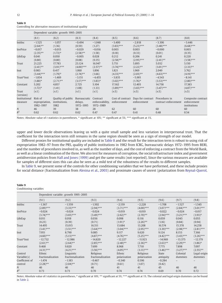
Table 8Controlling for alternative measures of institutional quality


(8.1) (8.2) (8.3) (8.4) (8.5) (8.6) (8.7) (8.8)

InitInc −1.525 −1.057 −0.494 −1.048 −3.400 −2.818 −3.306 −3.446(2.64)⁎⁎ (1.36) (0.59) (1.27) (3.83)⁎⁎⁎ (5.23)⁎⁎⁎ (3.48)⁎⁎⁎ (6.68)⁎⁎⁎

InvPrice −0.017 −0.015 −0.029 −0.016 0.003 0.003 −0.000 0.003(2.35)⁎⁎ (1.72)⁎ (2.58)⁎⁎ (1.58) (0.18) (0.33) (0.01) (0.35)

LifeExp 0.041 0.050 −0.005 0.028 0.212 0.206 0.241 0.220(0.80) (0.80) (0.08) (0.35) (2.58)⁎⁎ (2.95)⁎⁎⁎ (2.41)⁎⁎ (3.58)⁎⁎⁎

Trust 21.225 17.783 23.124 16.947 5.751 5.895 5.032 5.150(2.41)⁎⁎ (3.91)⁎⁎⁎ (4.00)⁎⁎⁎ (2.57)⁎⁎ (3.74)⁎⁎⁎ (2.22)⁎⁎ (3.01)⁎⁎⁎ (2.33)⁎⁎

Inst 0.983 0.417 1.060 1.896 1.821 1.969 2.049 3.762(3.44)⁎⁎⁎ (1.79)⁎ (2.74)⁎⁎ (1.66) (4.33)⁎⁎⁎ (2.03)⁎⁎ (4.63)⁎⁎⁎ (4.19)⁎⁎⁎

Trust⁎Inst −1.834 −1.469 −3.151 −4.455 −3.835 −5.901 −4.543 −8.141(1.88)⁎ (2.71)⁎⁎ (3.17)⁎⁎⁎ (1.83)⁎ (3.02)⁎⁎⁎ (1.76)⁎ (3.53)⁎⁎⁎ (2.80)⁎⁎⁎

Constant 5.202 4.857 2.725 5.104 17.162 12.403 14.758 17.383(1.72)⁎ (1.41) (1.08) (1.33) (3.89)⁎⁎⁎ (3.65)⁎⁎⁎ (3.47)⁎⁎⁎ (4.87)⁎⁎⁎

Trust(version)

(v.1) (v.1) (v.1) (v.1) (v.5) (v.5) (v.5) (v.5)

Institutionalmeasure

Risk ofexpropriation,1982–1997

Quality of publicinstitutions,1982

Bureaucraticdelays,1972–1995

Contractenforceability,1972–1989

Cost of contractenforcement

Days for contractenforcement

Procedures incontract enforcement

Composite contractenforcementinstitutions

N 46 39 38 28 62 60 60 60R2 0.62 0.62 0.62 0.47 0.47 0.41 0.48 0.54

Notes: Absolute value of t statistics in parentheses, ⁎ significant at 10%; ⁎⁎ significant at 5%; ⁎⁎⁎ significant at 1%.


upper and lower decile observations leaving us with a quite small sample and less variation in interpersonal trust. That thecoefficient for the interaction term still remains in the same region should be seen as a sign of strength of our model.

Different proxies for institutional quality are included in Table 8 and the result for the interaction term is robust to using risk ofexpropriation 1982–97 from the PRS, quality of public institutions in 1982 from ICRG, bureaucratic delays 1972–1995 from BERI,and the number of procedures involved in, as well as the number of days, and the cost of enforcing a contract from theWorld Bank,as well as a linear combination of the three.We also test formeasures of corruption, the social infrastructure index and governmentantidiversion policies from Hall and Jones (1999) and get the same results (not reported). Since the various measures are availablefor samples of different sizes this can also be seen as a mild test of the robustness of the results to different samples.

In Table 9, we present some of the controls for other conditioning variables that we have performed, and these include proxiesfor social distance (fractionalization from Alesina et al., 2003) and proximate causes of unrest (polarization from Reynal-Querol,

Table 9Conditioning variables


(9.1) (9.2) (9.3) (9.4) (9.5) (9.6) (9.7) (9.8)

InitInc −1.367 −1.559 −1.502 −2.159 −2.228 −1.708 −1.527 −1.545(2.89)⁎⁎⁎ (3.33)⁎⁎⁎ (2.94)⁎⁎⁎ (3.71)⁎⁎⁎ (4.00)⁎⁎⁎ (3.07)⁎⁎⁎ (2.84)⁎⁎⁎ (3.01)⁎⁎⁎

InvPrice −0.024 −0.024 −0.024 −0.019 −0.019 −0.022 −0.024 −0.017(3.74)⁎⁎⁎ (3.65)⁎⁎⁎ (3.49)⁎⁎⁎ (2.62)⁎⁎ (2.70)⁎⁎ (2.94)⁎⁎⁎ (3.21)⁎⁎⁎ (1.93)⁎

LifeExp 0.011 0.018 0.036 0.098 0.116 0.059 0.045 0.055(0.23) (0.39) (0.71) (1.91)⁎ (2.26)⁎⁎ (1.16) (0.84) (0.94)

Trust 14.495 15.015 16.511 13.684 13.208 16.574 15.378 14.258(3.41)⁎⁎⁎ (3.51)⁎⁎⁎ (3.64)⁎⁎⁎ (3.04)⁎⁎⁎ (2.95)⁎⁎⁎ (3.39)⁎⁎⁎ (2.98)⁎⁎⁎ (2.81)⁎⁎⁎

Inst 7.951 8.790 9.085 9.117 9.620 9.124 8.153 7.366(4.60)⁎⁎⁎ (5.13)⁎⁎⁎ (4.87)⁎⁎⁎ (4.76)⁎⁎⁎ (5.25)⁎⁎⁎ (4.42)⁎⁎⁎ (3.43)⁎⁎⁎ (3.26)⁎⁎⁎

Trust⁎Inst −12.732 −12.986 −14.820 −12.227 −11.923 −14.969 −13.375 −12.179(2.61)⁎⁎ (2.64)⁎⁎ (2.85)⁎⁎⁎ (2.40)⁎⁎ (2.36)⁎⁎ (2.63)⁎⁎ (2.29)⁎⁎ (1.86)⁎

Constant 9.468 9.820 7.699 8.968 7.710 7.775 7.898 7.097(4.31)⁎⁎⁎ (4.21)⁎⁎⁎ (3.56)⁎⁎⁎ (4.05)⁎⁎⁎ (3.13)⁎⁎⁎ (3.46)⁎⁎⁎ (3.27)⁎⁎⁎ (2.55)⁎⁎

ControlVariable(s)

Ethnicfractionalization

Linguisticfractionalization

Religiousfractionalization

Ethnicpolarization

Religiouspolarization

Stateantiquity

Colonialdummies

Legal origindummies

Coefficient ofcontrol

−1.474 −1.183 −0.467 −0.340 0.596 −0.284 – –

(2.28)⁎⁎ (2.04)⁎⁎ (0.71) (0.61) (1.07) (0.42)N 46 46 46 41 41 45 46 46R2 0.73 0.73 0.70 0.74 0.74 0.69 0.70 0.72

Notes: Absolute value of t statistics in parentheses, ⁎ significant at 10%; ⁎⁎ significant at 5%; ⁎⁎⁎ significant at 1%. The colonial and legal origin dummies can be foundin Table 2.


2006), as well as proxies for historical factors such as state antiquity from Putterman (2006), legal origin, and identity of pastcolonial power.23 The main result remains intact and the magnitudes of the estimated coefficients are remarkably stable.

Finally, is it backwardness in the form of low income, rather than weak institutions, that gives a high return to social capital?Knack and Keefer (1997) and Zak and Knack (2001) interact initial income and trust and get a significant and negative coefficientwhen regressing growth 1980–1992, and both growth and investment share 1970–1992 respectively. Whereas Knack and Keefer(1997) propose that this implies that trust is more needed where contracting institutions are weak (without providing anyevidence that this is the mechanism that makes the interaction term negative), Zak and Knack (2001) argue that the result impliesthat backwardness is more of an advantage in high-trust countries.

Whenwe interact trust with income instead of with institutions we also obtain a negative and significant interaction term.24 Inan attempt to find out which mechanism is the stronger one, we included both the interaction of income and trust and theinteraction of institutions and trust. In our growth regression the result is that neither of them enters significantly, but wheninvestment rate is the dependent variable the interaction between trust and institutions continue to be estimated with precision.One should not overinterpret the results from this kind of exercise but a reasonable interpretation is that if anything it is the level offormal institutions rather than the level of income that matters for the effect of trust on economic performance.

4. Concluding remarks

This paper provides new insights into the current debate about the roles of social capital and institutions in economicdevelopment. Arguing that there is a missing link from micro studies to macro studies of social capital, it presents a simpletheoretical framework and cross-country evidence showing that the effect of social capital on economic growth, as well as on theinvestment rate, is nonlinear and dependent on the quality of formal institutions. More specifically, it shows that social capitalmatters the most when formal institutions are weak and almost ceases to matter when institutions are strong.

For example, a one standard deviation increase in social capital is estimated to increase the growth rate by 1.8 percentage pointsin Nigeria but only by 0.3 percentage points in Canada, which is in sharp contrast to earlier cross-country studies that argue thatsocial capital always improves economic growth. This implies that present attempts at building social capital creates, if successful, astrong pro-growth potential for poor countries with bad institutions. Concerns have been raised that social capital is waning in thewesternworld and that this will have economic consequences. The findings presented in this paper imply that as long as the formalinstitutions are kept strong, these concerns are premature. Though the Canada–Nigeria example should be regarded as anillustration, the general results are highly robust to a number of different specifications in the basic variables.

TheWorld Bank has made large efforts at promoting better formal institutions in developing countries and also, in recent years,begun focusing on building social capital as well. Efforts aimed at building social capital is conducted in community-level projects.However, the extent to which these efforts have been successful is rather unclear (World Bank, 2005). Our results indicate thatmuch could be gained by making these projects work in areas with poor institutions.

Furthermore, much of the scholarly debate evolves around social capital and formal institutions as either mainly substitutes orcomplements. The result of this paper suggests that the relationship is mainly about substitution. However, unlike some of theprevious literature, the paper does not discuss or test for any dynamic process between the variables. The deeper determinants, aswell as the evolution of the relationship over time, are still largely unresolved issues and provide potential avenues for fruitfulresearch, both theoretical and empirical.

Acknowledgements

We gratefully acknowledge helpful comments from Arne Bigsten, Fredrik Carlsson, Shon Ferguson, Heather Congdon Fors,Martin Dufwenberg, Marcel Fafchamps, Nicola Gennaioli, Olof Johansson-Stenman, Katarina Nordblom, Sjak Smulders, JakobSvensson, David von Below, seminar participants at University of Gothenburg, Tilburg University, Växjö University, and the EUDNWorkshop in Paris, two anonymous referees, and the editor of this journal. Olssonwould like to thank Vetenskapsrådet, SIDA, andthe Wallander-Hedelius Foundation for financial support.

References

Acemoglu, D., Johnson, S., 2005. Unbundling institutions. Journal of Political Economy 113, 949–995.Acemoglu, D., Johnson, S., Robinson, J., 2001. The colonial origins of comparative development: an empirical investigation. American Economic Review 91,

1369–1401.Acemoglu, D., Johnson, S., Robinson, J., 2002. Reversal of fortune: geography and institutions in the making of the modern world income distribution. Quarterly

Journal of Economics 117, 1231–1294.Ahlerup, P., Olsson, O., Yanagizawa, D., 2007. Social capital vs institutions in the growth process. Extended working paper version available at bhttp://www.hgu.gu.

se/item.aspx?id=2465N.Alesina, A., Devleeschauwer, A., Easterly, W., Kurlat, S., Wacziarg, R., 2003. Fractionalization. Journal of Economic Growth 8, 155–194.Banerjee, A., Iyer, L., 2005. History, institutions, and economic performance: the legacy of colonial land tenure systems in India. American Economic Review 95,

1190–1213.

23 We have also tried to include various measures of openness to trade (exports plus imports as a share of GDP) but these turned out to have insignificantestimates and did not affect the parameter for our key interaction term. Documentation of these results is available upon request.24 See Ahlerup et al. (2007) for the details of this exercise.

http://www.hgu.gu.se/item.aspx?id=2465

http://www.hgu.gu.se/item.aspx?id=2465


Beckmann, V., Roger, S., 2004. Courts and contract enforcement in transition agriculture: theory and evidence from Poland. Agricultural Economics 31, 251–263.Beugelsdijk, S., 2006. A note on the theory and measurement of trust in explaining differences in economic growth. Cambridge Journal of Economics 30, 371–387.Beugelsdijk, S., 2008. Trust, institutions, and the ‘generally speaking question’: a reply to Uslaner. Cambridge Journal of Economics 32, 633–638.Beugelsdijk, S., Smulders, S., 2004. Social capital and growth. Tilburg University, mimeo.Beugelsdijk, S., van Schaik, A., 2005. Social capital and growth in European regions: an empirical test. European Journal of Political Economy 21, 301–324.Beugelsdijk, S., de Groot, H., van Schaik, A., 2004. Trust and economic growth: a robustness analysis. Oxford Economic Papers 56, 118–134.Bigsten, A., Collier, P., Dercon, S., Fafchamps, M., Gauthier, B., Gunning, J.W., Oduro, A., Oostendorp, R., Patillo, C., Söderbom, M., Teal, F., Zeufack, A., 2000. Contract

flexibility and dispute resolution in African manufacturing. Journal of Development Studies 36, 1–37.Bjornskov, C., 2006. The multiple facets of social capital. European Journal of Political Economy 22, 22–40.Brennan, G., Guth, W., Kliemt, H., 2003. Trust in the shadow of the courts. Journal of Institutional and Theoretical Economics 159, 16–36.Brock, W., Durlauf, S., 2001. Growth empirics and reality. The World Bank Economic Review 15, 229–272.CEPII. 2006. Available online at http://www.cepii.fr, baccessed 20060520N.CID, 2001. Gallup, Mellinger, and Sachs, GEOGRAPHY DATASETS. Center for International Development, Harvard University. Available online at http://www.cid.

harvard.edu.Congdon Fors, H., Olsson, O., 2007. Endogenous institutional change after independence. European Economic Review 51, 1896–1921.Durlauf, S.N., 2002. On the empirics of social capital. The Economic Journal 112, 459–479.Durlauf, S.N., Fafchamps, M., 2005. Social capital. In: Aghion, P., Durlauf, S.N. (Eds.), Handbook of Economic Growth, vol. 1B. North-Holland, Amsterdam.Fafchamps, M., Minten, B., 2002. Returns to social network capital among traders. Oxford Economic Papers 54, 173–206.Francois, P., Zabojnik, J., 2005. Trust, social capital, and economic development. Journal of the European Economic Association 3, 51–94.Glaeser, E.L., La Porta, R., Lopez-de-Silanes, F., Shleifer, A., 2004. Do institutions cause growth? Journal of Economic Growth 9, 271–303.Greif, A., 1993. Contract enforceability and economic institutions in early trade: the Maghribi traders' coalition. American Economic Review 83, 525–548.Greif, A., 2006. Institutions and the path to the modern economy. Cambridge University Press, Cambridge.Grootaert, C., Narayan, D., 2004. Local institutions, poverty and household welfare in Bolivia. World Development 32, 1179–1198.Guiso, L., Sapienza, P., Zingales, L., 2004. The role of social capital in financial development. American Economic Review 94, 526–556.Guth, W., Ockenfels, A., 2005. The coevolution of morality and legal institutions: an indirect evolutionary approach. Journal of Institutional Economics 1, 155–174.Hall, R.E., Jones, C.I., 1999. Why do some countries produce so much more output per worker than others? The Quarterly Journal of Economics 114, 83–116.Heston, A., Summers, R., Aten, B., 2006. Penn World Table Version 6.2. Center for International Comparisons of Production, Income and Prices, University of

Pennsylvania.Johnson, S., McMillan, J., Woodruff, C., 2002. Courts and relational contracts. Journal of Law, Economics, and Organization 18, 221–277.Knack, S., Keefer, P., 1995. Institutions and economic performance: cross-country tests using alternative institutional measures. Economics and Politics 7, 207–225.Knack, S., Keefer, P., 1997. Does social capital have an economic payoff? A cross-country investigation. Quarterly Journal of Economics 112, 1251–1288.Krishna, A., 2001. Moving from the stock of social capital to the flow of benefits: the role of agency. World Development 29, 925–943.La Porta, R., Lopez-de-Silanes, F., Schleifer, A., Vishny, R., 1997. Trust in large organizations. The American Economic Review 87, 333–338.Levine, R., Renelt, D., 1992. A sensitivity analysis of cross-country growth regressions. American Economic Review 82, 942–963.McMillan, J., Woodruff, C., 1999. Dispute prevention without courts in Vietnam. Journal of Law, Economics, and Organization 15, 637–658.Miguel, E., Gertler, P., Levine, D.I., 2005. Does social capital promote industrialization? Evidence from a rapid industrializer. Review of Economics and Statistics 87,

754–762.North, D., 1981. Structure and Change in Economic History. W.W. Norton & Co., New York.North, D., 1990. Institutions, Institutional Change, and Economic Performance. Cambridge University Press, Cambridge.Nuxoll, D.A., 1994. Differences in relative prices and international differences in growth rates. American Economic Review 84, 1423–1436.Putterman, L., 2006. Dataset available online at http://www.econ.brown.edu/fac/Louis_Putterman, baccessed 20060407N.Reynal-Querol, M., 2006. Available online at http://tornasol.upf.es/reynal/data_web.htm, baccessed 20061106N.Rothstein, B., 2000. Social Traps and the Problem of Trust. Cambridge University Press, Cambridge.Staiger, D., Stock, J.H., 1997. Instrumental variables regression with weak instruments. Econometrica 65, 557–586.Stock, J.H., Yogo, M., 2002. Testing for weak instruments in linear IV regression. NBER Technical Working Paper No. 284.Tabellini, G., 2006. Culture and institutions: economic development in the regions of Europe. Bocconi University, mimeo.Temple, J., 1999. The new growth evidence. Journal of Economic Literature 37, 112–156.Teorell, J., Holmberg, S., Rothstein, B., 2006. The Quality of Government Dataset, version 15, Nov06. Göteborg University, Available online at http://www.qog.pol.gu.se,

baccessed 20061108N.Uslaner, E.M., 2008. The foundations of trust: macro and micro. Cambridge Journal of Economics 32, 289–294.World Bank, 2005. The effectiveness of World Bank support for community-based and -driven development: an OED evaluation. Available online at http://www.

worldbank.org/oed/cbdcdd.World Bank, 2006a. World Development Indicators Online. Available online at http://www.worldbank.org, baccessed 20061106N.World Bank, 2006b. Doing Business. Available online at http://www.doingbusiness.org, baccessed 20061027N.WVS, 2006. World Values Survey. Available online at http://www.worldvaluessurvey.org, baccessed 20061106 N.Zak, P.J., Knack, S., 2001. Trust and growth. The Economic Journal 111, 295–321.

http://www.cepii.fr

http://www.cid.harvard.edu

http://www.cid.harvard.edu

http://www.econ.brown.edu/fac/Louis_Putterman

http://tornasol.upf.es/reynal/data_web.htm

http://www.qog.pol.gu.se

http://www.worldbank.org/oed/cbdcdd

http://www.worldbank.org/oed/cbdcdd

http://www.worldbank.org

http://www.doingbusiness.org

http://www.worldvaluessurvey.org

The Roots of Ethnic Diversity

Pelle Ahlerup�

University of Gothenburg

Ola OlssonUniversity of Gothenburg

September 2009

Abstract

The level of ethnic diversity is believed to have signi�cant consequences for

economic and political development within countries. In this paper, we provide

a theoretical and empirical analysis of the determinants of ethnic diversity in the

world. We introduce a model of cultural and genetic drift where new ethnic groups

endogenously emerge among peripheral populations in response to an insu¢ cient

supply of public goods. In line with our model, we �nd that the duration of hu-

man settlements since prehistoric times has a strong positive association with ethnic

diversity. Ethnic diversity further decreases with the length of modern state experi-

ence and with distance from the equator. Both �evolutionary�and �constructivist�

hypotheses of ethnic fractionalization thus receive some support.

Keywords: ethnic diversity, ethnicity, human origins.

JEL classi�cation: N40, N50, Z10

1 Introduction

It is widely agreed that ethnic cleavages within countries can have far-reaching conse-

quences for political processes and economic development. Accepting this observation

naturally leads to the question: Why are some countries more ethnically fractionalized

than others? For instance, why is the probability that two randomly chosen individu-

als belong to di¤erent ethnic groups only 0.2 percent in South Korea whereas the same

probability is roughly 93 percent in Uganda?1

�Dept. of Economics, University of Gothenburg, Box 640, 405 30 Gothenburg, Sweden. Email:[email protected]. We have received useful comments from Carl-Johan Dalgaard, SteliosMichalopoulos, Andrea Mitrut, Karl-Ove Moene, Brian Wood, and seminar participants at the Universityof Copenhagen, the University of Gothenburg, Lund University, the EEA meetings in Milan, and theNordic Workshop in Development Economics. A special thanks also to Louis Putterman for generouslysharing data with us. Olsson gratefully acknowledges �nancial support from SIDA, Vetenskapsrådet, andthe Wallander-Hedelius foundation.

1The estimates are taken from Alesina et al. (2003).

1

The broad aim of this paper is to o¤er theory and evidence to improve our understand-

ing of the determinants of ethnic diversity across the world. We explore the explanatory

power of two main hypotheses regarding the formation of ethnic identities: the construc-

tivist view, arguing that ethnic identi�cations are primarily a product of state formation

processes during modernity, and the evolutionary view, contending that ethnic divisions

have deep roots in history and ecology and should be analyzed in an evolutionary frame-

work. A key prediction from our evolutionary model of ethnicity is that the antiquity

of uninterrupted human settlement in a given area should be positively correlated with

current levels of ethnic fractionalization in that area. The intuition behind this hypoth-

esis is that among prehistoric hunter-gatherer populations, random genetic and cultural

drift that accumulated over time repeatedly caused new groups to form in order to secure

an e¢ cient provision of public goods. We argue that the ethnic legacy from prehistory

should still be detectable in the current distribution of ethnic groups.

In order to empirically identify this e¤ect, we use recent research on the human genome

to develop a new variable that captures the duration of settlement by modern humans for

all countries in the world. The hypothesis of a positive e¤ect of the duration of human

settlements on ethnic diversity receives strong empirical support, also when we control

for other proxies for human settlement duration and other relevant factors. In fact, the

settlement duration variable alone explains more than a fourth of the total cross-country

variation in ethnic diversity. We also �nd, in line with the constructivist view, that various

indicators of state history tend to increase ethnic homogeneity, and that ethnic diversity

decreases with distance from the equator. Our results have particular relevance for the

highly fractionalized African countries. Although factors such as the very long presence

of humans, the proximity to the equator, and the lack of historical state experience all

serve to explain the current high level of ethnic diversity in Africa, our results also suggest

that fractionalization should decrease with time as states mature.

Our work is motivated by a large literature in social science on the political and

economic impacts of ethnic diversity. In economics, an early in�uential study is Easterly

and Levine (1997), who show that the high degree of ethnic fractionalization in Africa

could explain a large part of the continent�s dismal growth performance. There is however

a widespread notion that the negative association between ethnic fractionalization and

growth is not uniform. Collier (2000) �nds it only in nondemocratic countries and Easterly

(2001) claims that the e¤ect is weaker where institutional quality is higher. Alesina and

La Ferrara (2005) con�rm Easterly and Levine�s (1997) basic results and �nd that the

negative e¤ect is less pronounced in rich countries, and that after controling for this e¤ect

the impact of democracy is nonsigni�cant. Moreover, ethnically fractionalized countries

tend to be more corrupt and have longer bureaucratic delays, as well as weaker provision of

public goods such as infrastructure, school attainment, and health (La Porta et al., 1999;

Alesina et al., 2003). The provision of public goods in ethnically diverse societies tends to

2

be biased toward excludable goods rather than non-excludable goods such as education

and defense (Alesina and Wacziarg, 1998; Kimenyi, 2006). Dimensions of ethnic diversity

have also been discussed in conjunction with civil wars and political instability (Collier

and Hoe er, 2004). The increased scholarly interest in the e¤ects of ethnic diversity

stimulated the creation of two new indices on ethnic fractionalization, namely the ones

by Alesina et al. (2003) and Fearon (2003).2 In our empirical section, we use the index

created by Alesina et al. (2003), although our results are robust to using Fearon�s (2003)

index as well.

In political science and sociology, a rich tradition has studied the sources of ethnicity

as well as the impact of ethnicity on state formation and other historical developments.

In the constructivist literature, ethnic identi�cation is basically regarded as a socially

constructed phenomenon appearing during modernity (since circa 1800) for the purpose

of uniting disparate nations into states (Gellner, 1983; Anderson, 1983; Hobsbawm and

Ranger, 1983). The vehicles for the achievement of nation-states were to be found in a

combination of e¢ cient printing technology, universal literacy, and industrialization that

broke up traditional societies.

What we refer to as the evolutionary tradition, on the other hand, is a class of theories

with the common feature that they regard ethnic identi�cation as a natural and evolution-

arily successful behavior that has existed throughout history.3 In van den Berghe�s (1981,

1995) sociobiological model of ethnicity, ethnic groups are regarded as extended kinships

that are successful as a means of social organization because cooperation based on kin

has evolved as an evolutionary favorable strategy for solving collective action problems.

Dawkins (1976) also sees a close connection between the evolution of genes and of cultural

traits or behaviors, which he refers to as �memes.�Just like genes, memes (such as modes

of social organization) are subject to mutation, natural selection, and random drift.4

The evolutionary view has obvious links to current advances in genetic research, which

is another building block of our analysis. The rapid progress in this area has drastically

changed the scienti�c community�s view on how the world was populated in prehistoric

times, and also sheds light on how di¤erent ethnic groups are related genetically (Oppen-

heimer, 2003). This path-breaking research on the human genome has so far had very

little impact in social science.

The level of ethnic diversity is almost always taken as a given in economics. A recent

exception to this is Leeson (2005), who argues based on historical examples that colonial

policy was often purposely designed to increase ethnic fractionalization. In an interesting

2Alesina and La Ferrara (2005) provide a comprehensive overview of much of this literature.3We include the so-called �primordial view� of ethnicity in this category of works, associated with,

e.g., Shils (1957). See Smith (1986) for a nice overview of the arguments.4Dawkins (2006) suggests that a particular cultural attribute of ethnic identi�cation �religion �has

emerged through natural selection as an unintended by-product of the evolutionarily successful strategyfor children to obey parents and believe in (without questioning) narratives that elders tell. The di¤erentvariants of religious behavior are however probably due to random drift.

3

study of neighboring communities in Kenya and Tanzania, Miguel (2004) shows that

governments in former colonies might have an important role to play in fostering a national

identity over tribal identi�cation.

In a theoretical model of ethnic con�ict, Caselli and Coleman (2006) propose that

people on the losing side of a con�ict might switch ethnicity endogenously if the costs of

switching are not too high. Our modeling framework is more closely related to Alesina

and Spolaore (1997, 2003), where the decision to break up or form nations (rather than

ethnic groups, as in our case) is modeled as a trade-o¤ between economies of scale and

preference heterogeneity.5 More speci�cally, we provide a micro model of �ethnogenesis,�

in which genetic and cultural drift over time increases cultural distances among people

and causes the public goods provision from the core to the periphery to deteriorate.

Despite the widespread recognition of the importance of ethnicity in politics and eco-

nomic development, we are aware of only one other systematic attempt to account for

the international variation in ethnic diversity. In a current working paper, Michalopou-

los (2008) argues that geographical variation in a given area should reduce inter-regional

migration and lead to more ethnic groups.6 This prediction concerning the role of geo-

graphical friction receives empirical support in a cross-country analysis and in a study

of a large number of adjacent pairs of regions. Our approach di¤ers in some important

ways from that of Michalopoulos (2008), especially in that our theory of ethnic diversity

is centered on public goods provision and on cultural drift, rather than on human capital

transmission. Furthermore, our empirical focus is on the time since original settlement,

which we �nd strong support for in the empirical analysis.7

The only other papers that also explicitly takes into account genetic and/or cultural

evolution in a long-run perspective is Spolaore and Wacziarg (2006) and Ashraf and Galor

(2008). Using data on genetic distances between populations from Cavalli-Sforza et al.

(1994), Spolaore and Wacziarg show that income convergence appears to be faster among

genetically �close�countries and peoples due to a stronger di¤usion of technology. Ashraf

and Galor (2008) argue that there is a trade-o¤ in how the level of genetic variation in

populations within countries a¤ects economic performance. On the one hand, more genetic

variation should make an intergenerational transmission of human capital more di¢ cult.

On the other hand, more diversity should improve the creation of new technological ideas.

Using data on genetic diversity (heterozygosity) within countries, Ashraf and Galor (2008)

demonstrate that there appears to have been an inverted U-shaped relationship between

diversity and economic performance in 1500 AD. Our approach di¤ers from those above

5There is also literature on social distance and social identity, e.g., Akerlof (1997) and Akerlof andKranton (2000), that shares our basic notion that cultural proximity plays an important role in politicaland economic decisions.

6See also Ashraf and Galor (2007) for a model where geography has an important e¤ect on the levelof cultural assimilation.

7Our empirical analysis also shows that there is an important role for geographical diversity, as pre-dicted by our own model and by Michalopoulos (2008).

4

in that our ultimate dependent variable is ethnic fractionalization rather than economic

performance.

The above brief literature overview suggests that our paper makes at least three con-

tributions to the existing literature: First, we are the �rst to o¤er a public goods-based

model of endogenous ethnic group formation with genetic and cultural drift as the engine

of ethnic fractionalization. Second, our paper provides the �rst attempt at measuring the

duration of uninterrupted human settlement in a cross-country setting. Third, we provide

a comprehensive empirical assessment of the determinants of ethnic diversity across the

world. Our main �ndings in this regard are that the timing of initial settlement by modern

humans still can explain a large fraction of existing di¤erences in ethnic fractionalization

and that state experience during modernity is another key factor.

The paper is structured as follows. In Section 2, we argue that the diverse literature on

the constructivist and evolutionary explanations can be combined with recent ecological

and genetic research into one joint framework for understanding ethnic diversity. In

Section 3, we outline our model of ethnic fractionalization. In Section 4, we brie�y discuss

the construction of our measures for the duration of human settlements and present our

empirical strategy. Section 5 outlines the main empirical results, and Section 6 concludes

the paper.

2 Literature overview

In this section we discuss the main theories on the evolution of ethnic diversity in some

detail. An ethnic group is a social entity with two basic features: (1) the group members

have a shared belief in a common history or ancestry, often associated with a homeland,

a founding migration, or a settlement of new territory, and (2) the group currently forms

a cultural community, manifested for instance in a common language and religion and

shared customs. There is usually also a sense of solidarity among members (Fearon, 2003;

Bates, 2006). Ethnicity is distinct from concepts such as race and nation. Although both

latter terms are generally poorly de�ned in the literature, race usually refers to physical

distinguishing features such as skin color, hair texture, or stature. The concepts of nation

and nationalism, on the other hand, are also based on notions of a shared ancestry and

a cultural community, yet most authors consider nationalism to be a concept primarily

to be used in conjunction with discussions on (nation-)state formation during modernity

(Gellner, 1983).

2.1 The evolutionary view

At the core of the evolutionary view lies an emphasis on the history and origins of ethnic

groups. Smith (1986) contends that nations and ethnic identi�cation have been in place

5

at least since the emergence of the �rst civilizations. Already in the late third millennium

BC, there was a system of states in the Near East based on ethnic core populations,

including the Egyptian and Sumerian civilizations. Now, if fully developed nation-states

with distinct written languages, religions, customs, and traditions were in place in the

Near East as early as 3000 BC, where did they originate from?

One potential explanation is provided by the sociobiological theory of ethnic origins,

associated mainly with Edward Shils (1957) and Pierre van den Berghe (1981, 1995).

Firmly rooted in evolutionary biology, van den Berghe develops a model of ethnicity as

�extended kinship.�The basis for the argument is that humans, like other mammals, are

by nature nepotistic, favoring kin in the daily struggle for survival (Jones, 2000). By the

evolutionary logic, given a lifetime budget constraint of time and energy, an individual

has a greater chance of passing on her genes to future generations if she invests all her

resources in her o¤spring and family, rather than if she spends her time and e¤ort on

unrelated people. This means that nepotistic genotypes will generally have a greater

reproductive success and tend to dominate all populations.

The nepotism argument applies also to members of the extended family since they also

carry one�s genes, though not to the same extent as direct o¤spring. The evolutionary

logic dictates that individuals develop a sense of loyalty with their close family, their

extended family, their clan, and so on. Since extended kinships eventually become very

large and since it is usually hard to distinguish kin just by physical appearance, particular

cultural markers such as dialects, customs, and traditions evolve in order to di¤erentiate

from �the others.�Such behavioral traits can be analyzed within the same evolutionary

framework as genetics (Dawkins 1976). Over generations, extended families evolve to

become ethnic groups.

Nepotistic individuals who organized in extended family groups had an advantage in

having an e¢ cient mechanism for sustaining collective action. Family ties restricted free-

riding behavior and provided an informal rule-based system in the absence of codi�ed

law or a ruling elite. Family networks supplied selective disincentives against cheating on

delivering collective goods. In line with this logic, we conjecture that a primary reason

for the existence of ethnic groups is their role in organizing the provision of public goods.8

A straightforward implication of the evolutionary view is that we should expect that

distinguishable extended kinships of the type described above have existed throughout

most of human history. It is by now generally agreed that the history of �anatomically

modern humans�(AMH) goes back roughly 200,000 years.9 Genetic research on human

origins suggests that all human beings in the world today originate from a founding

8It has recently been suggested that cultural in-group markers such as religion might have emerged asa way of protecting groups from being subject to infectious disease (Fincher et al., 2008).

9The oldest fossil of an AMH is the so-called Omo I skeleton retrieved from a site in Kibish insouthwestern Ethiopia. It was recently dated to be approximately 195,000 years old (McDougall et al.,2005).

6

population of a few thousand individuals in East Africa (Oppenheimer, 2003).

As AMH migrated from their East African home to other parts of sub-Saharan Africa,

they started an inevitable process of ethnic and genetic fractionalization. Since public

goods could not be e¤ectively provided over long distances, groups necessarily organized

in small units. A result of this process was genetic and cultural drift. Genetic drift is a

general tendency for genetic diversity to be reduced among small and relatively isolated

populations as time passes. If there were initially for instance �ve lineages in a founding

group �labeled A, B, C, D, and E �there could after say ten generations be only the D-

lineage, hence all subsequent o¤spring had D as their ancestor. As we shall see, although

genetic drift is a random process, the rate at which it occurs has an estimated expected

value.10 Cultural drift is in an analogous manner the tendency for multiple cultural traits

to be reduced within an isolated population. Cultural drift implies that two groups that

initially shared the same culture should, after a number of generations in isolation, display

two quite distinct sets of cultural characteristics, often di¤erent enough for all parties to

recognize them as two di¤erent ethnic groups (Cavalli-Sforza et al., 1994). However,

genetic and cultural drift does not only occur between groups, it is also present within

groups, and can emerge over time as a result of clustering at for instance the village level

when there is little interbreeding between villages. Eventually, such drift causes even

non-migrating peoples to form distinct ethnic groups. A concept closely related to drift

is the �founder�s e¤ect,�which arises when a small fraction of the whole population move

on to establish a new colony. This smaller group will naturally have a lower degree of

genetic variation than the larger remaining population.11

In order to get an idea of what such a fractionalized prehistoric society might have

looked like, it is illustrative to consider Papua New Guinea (PNG), where isolated groups

have populated the greater part of the country to this day. In PNG, an estimated 820

di¤erent languages are currently spoken among its 5.6 million inhabitants (CIA, 2007).

Two factors appear to have contributed to this enormous diversity. First, PNG�s geogra-

phy is quite extreme with mountains and impenetrable rain forests where groups easily

became isolated. Second, PNG is believed to have been populated for some 65,000 years

and is therefore one of the countries with the longest continuous presence of AMH outside

Africa.

Our view of ethnic fractionalization thus implies that there should be strong linkages

between the formation of genetic and ethnic groups. The most intuitive reason for this is

of course that both cultural and genetic characteristics are essentially transmitted from

10A third factor behind genetic changes, distinct from migration and genetic drift, is natural selection.As observed by Dawkins (2006), the role of natural selection in the evolution of cultural expressions isunclear. For instance, it is not obvious why natural selection should give rise to di¤erences in linguisticor religious structures. Hence, Dawkins believes that most cultural traits have evolved through randomdrift.11Events such as population bottlenecks, where for some reason the population size is dramatically

reduced, can have the same e¤ect.

7

parents to children. Attempts at linking genetic and ethnic diversity into one framework

have previously been made outside economics. After the publication of Dawkins (1976),

a �eld of �memetics� has emerged where the evolution of cultural traits are analyzed

with the basic tools of Darwinian genetics. Empirically, it has been shown that linguistic

groups to some degree follow genetic patterns, suggesting �parallelism between genetic

and linguistic evolution�(Cavalli-Sforza et al., 1988: 6002). The development of mutually

unintelligible languages takes a mere 1,000 to 1,500 years if a population with a common

language is split into two groups (Cavalli-Sforza and Cavalli-Sforza, 1995). Recent research

by Dunn et al. (2005) on indigenous peoples in South Asia further suggests that there

are close links between the genetic relatedness among groups and di¤erences found in

language structure.

Recent studies on the human genome have produced genealogical trees showing how

related or genetically distant populations around the world are. Figure 1 shows one

such phylogenetic tree from Oppenheimer (2003), based on an often-cited study that uses

mitochondrial DNA from 53 individuals from around the world (Ingman et al., 2000). As

expected, the tree shows that the deepest genetic branches are found in Africa and that

all non-Africans descend from a branch that emerged relatively recently, i.e., some 83,000

years ago (L3). One of the most recent �ssions in the �gure occurred around 36,000 years

ago when the English, French, and Dutch individuals in the sample had their last common

ancestor down the female line. Based on the evidence above, we argue that since cultural

and genetic drift appear to be inevitable in all hunting-gathering societies, we should �nd

that territories with a long settlement history during prehistoric times are ethnically more

diverse than countries with a shorter settlement history, all other factors held constant.

2.2 The constructivist view

Contrasting the reasoning behind the evolutionary hypothesis, the constructivist discourse

points to a plethora of more recent factors with potential to a¤ect the current levels of

ethnic diversity. Figure 2 outlines some of these factors. The rise of Neolithic agriculture

was a dramatic turning point in human history. Initiated in the Fertile Crescent in the

Near East around 10,500 before present (BP), it spread westward to Europe and eastward

to the Indus Valley. In addition, independent transitions occurred in China (9,000 BP),

in South America (4,300 BP), and in a few other places (Smith, 1998; Putterman, 2008a).

From having been nomadic hunter-gatherers, people became sedentary farmers relying on

domesticated crops and animals. Sedentism and farming revolutionized human lives in

several aspects. Two of the most important changes were a large increase in population

growth and the introduction of a new class of specialists including warriors, craftsmen,

priests, and rulers (Diamond, 1997; Olsson and Hibbs, 2005).

On all continents, the rise of sedentary agriculture and a more strati�ed society was

8

relatively soon followed by the emergence of states (supratribal authority), writing, and

monumental structures resulting from grand collective e¤orts, such as the pyramids in

Egypt, Sumer, and Mexico; what is usually referred to as �civilization.�Gellner (1983)

argues that since the masses of farmers were relatively immobile and since literacy was only

reserved for a small elite, the type of cultural homogenization that took place in Europe

from the turn of the nineteenth century was not possible in the early civilizations. On the

other hand, Smith (1986) �nds that the ancient Sumerians �scattered around cities in the

densely populated Iraqi river plains �had a strong sense of a distinct ethnic identity with

a common language and religion, as had the Egyptians and many other peoples during

the same time in the Near East. In China, the state gradually incorporated surrounding

ethnic groups into the dominant Han culture (Diamond, 1997).

Numerous other more recent historical accounts of medieval and modern state forma-

tions in for instance France, Germany, and Spain also suggest that statehood experience

in general has had a homogenizing in�uence on culture and ethnic identity. A reasonable

conjecture from these observations is that within states, extended kinships partly lose

their raison d�être, i.e., the role as the most e¢ cient mode of organizing collective action

and the provision of public goods. State institutions like codi�ed law, courts, taxation,

and military protection substitute for the services provided by extended kinships, which is

the reason why many small ethnic groups disappear in such an environment. The implied

hypothesis is that the length of statehood experience, and the associated time since the

transition to agriculture and civilization, has a negative in�uence on ethnic diversity.

States have not only created institutions that have passively reduced heterogeneity,

but have also actively pursued policies designed to bring about more homogenous pop-

ulations. This process gained momentum when the modern industrial European states

at the turn of the eighteenth century acquired both the means and the motivation for

nation-building. The modern industrialized society�s increasing division of labor created,

in combination with a rapidly changing production, problems for which the creation of a

dynamic and mobile workforce was a solution. The industrial society required strangers

to easily communicate with and understand each other, and therefore demanded su¢ cient

homogeneity in both language and culture (Gellner, 1983).

The ambition to obtain an ability to wage and win wars was another driving force

behind the deliberate attempts to create homogenous populations. Referring to the Eu-

ropean experience, Tilly (1992:106) �nds that �rulers frequently sought to homogenize

their populations in the course of installing direct rule�because �within a homogenous

population, ordinary people were more likely to identify with their rulers, communication

could run more e¢ ciently, and an administrative innovation that worked in one segment

was likely to work elsewhere as well. People who sensed a common origin, furthermore,

were more likely to unite against external threats.�

In Europe, this process started well before the era of industrialization, when direct rule

9

replaced indirect rule by intermediaries. A high level of homogeneity in the population

was in fact both an ultimate result of the process and a factor making the process faster

and more e¤ective; it is easier to unite a population that is not too diverse to begin

with. The process whereby the European states encouraged national rather than ethnic

or local loyalty began in the eighteenth century, yet it was not until after the middle of

the nineteenth century that states forcefully began to expand into non-military activities

and populations increasingly came to view the state as the natural primary provider of

services previously provided at the local level.12

Another major historical event with potentially dramatic repercussions was European

colonialism from the �fteenth century onward. This heterogeneous process, coherently

analyzed in Osterhammel (2005) and Olsson (2007), is often thought to have had quite

disparate e¤ects depending on the time and duration of colonial dominance, the geog-

raphy of the area, and the initial wealth of the population. In stark contrast to the

homogenizing domestic policies of the time, the Europeans who ruled the colonial states

had no strong incentives to ethnically homogenize the colonial countries since these were

created only to bene�t the colonial power. On the contrary, �divide-and-rule�appeared

to be the most commonly used principle for keeping colonies under control, from the days

of Cortes�exploitation of ethnic con�icts during his conquest of the Aztec empire, to the

cynical di¤erential treatment of Hutus and Tutsis by the Belgians in twentieth century

Rwanda. However, during the colonization of the Americas, large segments of the popu-

lation were killed by the introduction of, for them, lethal diseases (Diamond, 1997) and

new population groups were forcefully introduced in the form of slaves of African descent.

Whether the overall result of the colonial era was increased or decreased ethnic diversity

is therefore an empirical issue.

2.3 Geography and ecology

The process of evolution is tied to the geographical context, and several micro-level factors

have the potential to in�uence the degree of ethnic diversity. A stylized fact from ecology

is that species richness, or diversity, is a product of isolation and adaptation, and that it

is greater closer to the equator. Studying pre-colonial North America, Mace and Pagel

(1995) �nd that language diversity follows the same latitudinal pattern as found for other

mammals and for birds. They also �nd that in this pre-colonial environment, linguistic

diversity was higher in areas with more habitat diversity.

Di¤erences in skin color alone do not create ethnic groups, but classi�cation of people

into groups may be easier where there are notable di¤erences in skin color, making the

formation and identi�cation of ethnic groups more rapid and detailed (Caselli and Cole-

12Tilly (1992:115-6) �nds that subnational loyalties and identi�cation withered as �states undertookto impose national languages, national education systems, national military service, and much more. [...]National symbols crystallized, national languages standardized, national markets organized.�

10

man, 2006). This implies that diversity within a country can be related to latitude, as

well as within-country di¤erences in latitude, humidity, and altitude, since paleoanthro-

pology and medical science have shown that variation in human skin color comes partly

from di¤erences in UV radiation, which in turn is determined by latitude, altitude, and

humidity. In fact, natural variations in UV radiation, with latitude and altitude, and

in precipitation can explain most of skin color variation (Chaplin, 2004). The residual

variation can to some degree be explained by quite recent migrations, where populations

have not yet had enough time to adjust (Diamond, 2005), which implies that similarity

of skin color is a weak predictor of close genetic connections (Jablonski, 2004).

The impact of latitude on ethnic diversity is complex. Cashdan (2001) �nds that the

correlation between the two is largely due to climatic variability, habitat diversity, and

pathogen loads. Where climate is variable and unpredictable, populations are forced to be-

come generalists and use wider ecological niches, and the presence of high pathogen loads

can, when local populations have adapted to them, be an isolating force by working both

as barriers to their own movement outside their territory and other populations�move-

ment into or conquest of the territory. Collard and Foley (2002) �nd that the number of

�cultures�within a certain area follows geographical patterns, i.e., falls with latitude, and

rises with temperature and rainfall, and that this pattern holds both in �new continents�

such as the Americas and �old continents�such as Africa.

A problem with geographical factors in our empirical study is that they are likely to

a¤ect our dependent variable both directly in a �biological�sense and indirectly through

their in�uence on society in general, as indicated in Figure 2. For instance, as emphasized

by Diamond (1997) and Olsson and Hibbs (2005), populations living in areas with a bio-

geography favorable for agriculture, e.g., riverine habitats with irrigation potential and

many suitable plants and animals for domestication, were the �rst to make the transition

and develop dense sedentary farming populations.13 A high population density entails less

isolation, ceteris paribus, and therefore less diversity. As mentioned above, the transition

to agriculture was usually soon followed by the formation of states (Chanda and Putter-

man, 2007). Hence, a high population density should have decreased ethnic diversity both

by decreasing isolation and by fostering statehood.

As any species spreads out from its origin, genetic diversity declines naturally due to

genetic drift and founder�s e¤ects, as discussed above. A popular hypothesis, developed in

more detail in Section 4.1, maintains that the �rst humans initially followed the coastlines

as they spread from Africa, with a beachcombing lifestyle, which means that areas closer

to the coast, and maybe waterways connected to it, were settled quite a long time before

the inland (Oppenheimer, 2003; Macauley et al., 2005). This suggests that coastal areas

13In the Near East, this biogeographic potential included the unusual abundance of grasses with aheavy kernel (such as the wild variants of wheat and barley) as well as many large and easily domesticatedmammals (such as the wild ancestors of sheep, goats, and cattle).

11

on the one hand could harbor more diverse populations due to their longer histories as

settlements. However, populations in these areas are less isolated. It is reasonable to

assume that over the millennia, the latter e¤ect should eventually come to dominate.

3 An evolutionary model of ethnic fractionalization

In this section, we brie�y develop a model of our key source of ethnic diversity: The

process of cultural drift among prehistoric populations who roamed the earth for most

of modern man�s history. The main building block of this model is our assumption that

ethnic groups are primarily a kinship-based type of social organization with the main

purpose of supplying public goods. Members of an initial group might potentially break

away and supply their own public goods if their distance to the core of the previous group

in terms of geography, kinship, or culture becomes too large. The main reasons to focus

the model on how the duration of settlements a¤ects ethnic diversity, rather than to also

incorporate other broad concepts such as state experience, colonialism and geography, is

that we believe that this concept is the most novel, and addresses issues that economists

are not generally acquainted with.

3.1 Basics

Let us assume an ethnic group of prehistoric hunter-gatherers whose population of size P

is uniformly spread along a one-dimensional geographical area of total size s. The area has

just been colonized by the group and no ��ssions�(split-ups of ethnic groups) have yet

occurred. Individuals in this group receive positive utility from consumption and leisure.

The primary reason that the ethnic group exists is to solve the collective action problem

inherent in public goods provision. The public good could, e.g., be primitive institutions

for hunting coordination, defense, dispute settlement, religious ceremonies, and exchange

of goods. What we have in mind is thus mainly intangible goods and services based

on mutual trust that are required for the community to stay together as an economic

unit. All members of the group have descended from a �founding father� and they all

therefore constitute an extended kinship. Cooperation among its members (kinship nepo-

tism) has evolved as an evolutionary favorable strategy throughout the history of human

development and is taken as given here.

The utility of each individual i 2 1; 2; :::; P is given by the utility function

Ui(ci; li) = � ln ci + (1� �) ln li; (1)

where ci is private consumption, li is leisure, and � 2 (0; 1) is a parameter. The loglinearform ensures diminishing marginal utility in each of the two arguments.

12

Consumption is the di¤erence between the value of individual production yi and the

individual contribution paid for the provision of the public good � i. For mathematical

convenience, we de�ne consumption as ci =yi� i> �c > 1. The ratio of production to

contributions must exceed a subsistence level �c, which in turn must obviously be greater

than unity. Only regions where this subsistence condition can be met will be populated.

Individual production yi is given by the production function

yi = gie i L

1� i ; (2)

where gi is the level of the public good that individual i bene�ts from, ei is the individual

e¤ort induced into production, Li is the land available to each individual, and 2 (0; 1)is an elasticity parameter that yields constant returns to scale in e¤ort and land. For sim-

plicity, we will normalize land to be Li = 1 for all i.14 Each individual�s total endowment

of time is normalized to unity, implying that li = 1� ei:

3.2 Public goods and cultural distance

The key factor in the model is gi, the e¤ective level of the public good experienced by

individual i. This level is

gi = g (1� �dimi (t)) � 0; (3)

where g is the level of the public good at its origin, � 2 [0; 1] is a parameter indicating thegeneral geographical frictions for the spatial di¤usion of the public good in the region, diis the geographical distance between individual i�s location and that where public goods

are produced, and mi (t) � 1 is a cultural distance function (of time t), speci�ed below.Starting with �, the parameter describes the general ruggedness of the terrain and

the physical di¢ culty of exchanging information, goods, and people. For instance, the

Nile River Valley has a small � since information and goods can very easily spread in

such a territory whereas the spatial frictions are much greater in tropical jungle areas or

mountainous terrains as in Papua New Guinea.

The distance from some individual i to the location of public good production didepends on the size of the area, s, and on where public goods are produced. In line with

Alesina and Spolaore (1997) and the Hotelling result, we assume that the provision of

public goods always takes place in the middle of the ethnic group�s territory. Obviously,

this is the location that is socially optimal given that we have local public goods that are

imperfectly spread over space. Defense considerations would also motivate a safe location

in the middle of the territory.15

14We implicitly assume that land is not an excludable, rival, or constraining factor for hunter-gatherersduring this era of very low population densities. While this is not an entirely realistic assumption, itallows us to focus on more central aspects.15The very common current location of capitals in the center of countries suggests that the logic of this

13

Initially, with only one ethnic group, the assumption of centrality implies that the

location of public goods production is s=2, i.e., in the middle of the total range s. Formally,

the distance from any location zi 2 [0; s] to the center is di =�� s2� zi

��. Hence, we musthave that di 2 [0; s=2]. Due to the uniform distribution of people across this territory,

the average member of the ethnic group will initially be located at a distance of s=4 from

the center. In order for gi to be positive at all di, we assume that levels are scaled such

that �di < 1.16 The fact that we specify an exact di is not meant to imply, however, that

people are sedentary. Their �location� on the line should simply be thought of as the

�average location�in their movements as nomadic hunter-gatherers.

Lastly, mi (t) � 1 re�ects internal cultural distance between the people at the centerand individual i within the group. This distance is an increasing function of time due to

genetic and cultural drift, as speci�ed further below. We assume that this process has

the general e¤ect of weakening the communication from the center and hence the e¤ective

level of the public goods enjoyed by individual i.17 In line with the arguments above, we

further assume that the process of genetic and cultural drift is one and the same.

Another key feature of our model is that even within the ethnic group, there are

subpopulations of varying sizes that live separated from each other in di¤erent segments

along s. Among hunter-gatherers, it is common that the basic economic unit is a band

or extended household of maybe 20-50 persons (Sahlins, 1972). We further assume that

such bands or clusters of bands practice assortative mating in the form of homogamy, i.e.,

they only breed within their own subpopulation of the ethnic group.18 Let us henceforth

refer to such a separate breeding cluster as a niche. The size of the population within

each niche is assumed to be identical and equal to N < P . For the sake of simplicity, we

also have that permanent migration to other niches is not possible, although information

can di¤use between them (with an e¢ ciency that depends on �).19

Given the isolation of the niches, they will be subject to genetic and cultural drifts that

move them socially apart, despite initially sharing a common cultural community. What

are the dynamics of the cultural distance function mi (t)? The basic dynamics of genetic

drift have been successfully characterized by genetic research. The general formula for

genetic distance between two separate populations is

Fst = 1� exp�� t

2�N

�; (4)

choice of location is indeed still important.16Inserting the extreme value di = s=2 further gives us that s� < 2.17One type of cultural drift that quickly emerges between separated populations is language change,

as discussed above.18This simplifying assumption only a¤ects the speed of the process. As long as homogamy is the

dominant form of mating in the niche the qualitative conclusions of the model stand.19We could have used a more relaxed assumption regarding migration, but it would have complicated the

model and potentially obscured our main point. See Michalopoulos (2008) for a model where geographicalfrictions in�uence migration patterns.

14

where Fst 2 (0; 1) is the genetic distance between the two populations, t is time (in

generations) since the two populations became separated, and � < 1 is the proportion of

the niche population who are of reproductive age (Cavalli-Sforza et al., 1994). Fst is thus

a positive, convex function of time. The expression shows that genetic drift also decreases

with the size of the reproducing population �N .20

In the analysis that follows, we assume that � = 1=2, i.e., that half the population is

of reproductive age. It can be shown that for relatively small values of t; the expression

for genetic drift and distance in (4) will be approximately linear with respect to time

(Cavalli-Sforza et al., 1994):

Fst �t

2�N=t

N: (5)

We assume that the number of niches q in the total area is PN= q such that q � 3 is

an odd integer. This simplifying assumption regarding the number of niches is made to

ensure that we have a core niche, c, where public goods are produced in the center. With

an even number of niches, the center must be located at a border between niches in order

to maintain a position of s=2. The fact that we have more than a single niche further

implies that there is scope for ethnic �ssions, as we shall see. The level of q might further

be seen as another measure of geographic diversity and of how naturally fractionalized a

territory is.21

The geographical extension of each niche is thus s=q. Population density, which is

identical along s, is �p. Hence,

N =P

q=s�p

q: (6)

As an illustration, let us consider an individual i who is located at some spot z < s=2,

i.e. to the left of the center, as shown in Figure 3a. The geographical distance to the

center is here di = s=2� z and q = 3. At z, i is not a member of the core niche c.Based on (5) and (6), we propose that the dynamic equation for cultural drift for any

individual i at location zi is

mi (t) =

(1 + Fst = 1 +

qtP

if zi =2 c1 otherwise.

(7)

In other words, individual i will experience cultural drift in relation to the core of the

ethnic group if i is not a member of the core niche, the latter being the equivalent to

the subset c on the real line. The level of drift outside the core niche will be the same

regardless of the number of other niches. If i is a member of the core niche, she will

20This is why a small founding population typically will experience rapid genetic drift, i.e., �foundere¤ect.�21It has for instance been suggested that a reason for the great diversity of peoples and nations on the

relatively small European continent is due to a natural split-up into many small core areas in betweenmountains and rivers (Jones, 1981).

15

experience no drift and mi (t) = 1. Note also that immediately when new groups emerge,

we will have that m (0) = 1, i.e., new group formation is always associated with cultural

consolidation even in the group or groups that remain in place.22

The structure outlined in (7) implies that the e¤ective level of public goods will be a

discontinuous function of geographical distance from the center, as illustrated in Figure

3b. When the boundary of the core niche is passed, gi will make a discontinuous jump

downward and get a more pronounced negative slope. The width of the jump will further

increase with time. Cultural drift thus gradually causes a deterioration in the e¤ective

supply of public goods, which, as we shall see, will make a �ssion event more and more

likely.

The total cost of providing the public good is k: In line with Alesina and Spolaore

(1997), we assume that each individual contributes the same to the provision of this good

� i = k=P , perhaps in the form of hunted game, artwork, or crafted goods. As above, P

is the size of the population in the area. For now, we will simply hold this level constant.

Making the fertility decision endogenous is straightforward but we refrain from that here

in order to keep the model simple. The fact that each individual�s contribution decreases

as the size of the population increases is a source of economies of scale.

3.3 The hunter-gatherer equilibrium

After having speci�ed all these functional forms, we can reformulate the utility function

as

Ui = � ln (g (1� �dimi) e i )� � ln

�k

P

�+ (1� �) ln (1� ei) :

We are also ready to study optimal individual behavior. The model has two stages,

and the individual�s �rst choice is whether to remain within the ethnic group where she

currently belongs or to form a new group together with her nearest neighbors. In the sec-

ond stage, the individual decides on optimal levels of e¤ort, leisure, and production within

the chosen group. The model is solved through backward induction and we therefore start

in the second stage.

By taking the usual �rst-order conditions for maximum, we can solve for the optimal

level of e¤ort e�: @Ui@ei= �

e�i� (1��)

1�e�i= 0. After some manipulations, the equilibrium levels

of e¤ort and leisure turn out to be e�i =�

1��+� and l�i =

1��1��+� . Note in particular

that the optimal level of e¤ort will be independent of the spatial frictions. The implied

22We believe that this assumption of cultural homogenization holds for most societies that experience asplit. If not, the dynamics of continued cultural fractionalization would have been very fast, a pattern thatwe do not seem to observe. Even without the homogenization assumption above, the central predictionregarding the in�uence of time on cultural distance would be qualitatively the same.

16

indirect level of utility is thus

Vi = ln

(� )� (1� �)1��

1� �+ �

!+ � ln (g (1� �dimi))� � ln

�k

P

�: (8)

The more complicated and crucial decision is made in the �rst stage. Taking the

second-stage level of utility into account, each individual considers whether she should

remain in the ethnic group or leave it and form a new one. We refer to the break-up of

one existing ethnic group into more than one group as an ethnic �ssion. The existence

of this kind of decision means that the core group is unable to prevent kinsmen from

breaking away; i.e., �ssion decisions can be made unilaterally even though such �ssions

cause a greater per capita cost of public goods for the kinsmen who stay in the old group.

We argue that this regime is the most reasonable for primitive hunter-gatherer societies

while it is not well applied to the later agricultural or industrial eras.

In our model, it is intuitively clear that an individual will be more inclined to form

a new ethnic group the greater the distance to the core and the greater the accumulated

level of cultural drift in her niche. Obviously, the people in the core, who are close to the

origin of public goods and to each other in terms of space and kinship, will never attempt

to form a new group since they have a small distance, belong to the same niche, and pay a

smaller contribution in the situation with one group than with two or more groups. Thus,

it will be people in the geographical periphery who will be the founders of new groups.

Formally, the decision hinges upon the relative indirect utilities from the two choices

for the people in the group�s most peripheral niche. The general mathematical condition

for an individual at any location zi in the most peripheral niche to the left to be willing

to form a new ethnic group is

V newi � Vi = � ln

0@�1� � �

�� s2q � zi�� sq�

1�mi� �� s2� zi

�� s1A > 0; (9)

where V newi is the indirect utility for i after having joined the new ethnic group and Viis the utility from status quo.23 As in the example above, let us assume that zi < s

2qso

that the absolute distance notation can be eliminated. (9) is satis�ed if the expression in

23In the expression above, it should be remembered that V newi is independent of the parameters inm since m (0) = 1. Also, g is identical in the two scenarios and therefore cancels out in the utilitycomparison.

17

parentheses exceeds unity or, analogously, if�1� �

�s

2q� zi

��s

q��1�mi�

�s2� zi

��s = (10)

s

�1

q� 1�

| {z }cost e¤ect (-)

+ s�

�mi

�s2� zi

�� 1q

�s

2q� zi

��| {z }

public good supply-e¤ect (+)

= (�;mi) > 0: (11)

In (11), the expression is broken up into two parts. The �rst part �the cost e¤ect �is

clearly negative and re�ects the increase in costs paid for public goods if i joins the new

group. The intuition is that there will then be a smaller population to share the �xed cost

k. This negative e¤ect of a �ssion is potentially dominated by the positive second part �

the public good supply-e¤ect �which re�ects the gains from a shorter e¤ective distance

to the center of the new group. These net gains with a new group will grow with time

due to internal cultural drift since mi(t) grows over time. The public good supply-e¤ect

is also enhanced by the level of spatial frictions �. The impact of the number of potential

niches q is ambiguous: On the one hand, a larger q makes each new group smaller and

increases average costs. On the other hand, a large q ensures that the distance to the new

center of public goods supply will be small.

The expression in (10) can form the basis for several di¤erent scenarios concerning

the collective decisions to break away and form new groups. Here, we will only consider

one of a whole class of potential decision regimes: That a new group will be formed if the

members of a peripheral niche unanimously agree to leave the old group. The symmetric

structure implies that this event occurs simultaneously in peripheral niches to the left and

to the right of the core group.24 Assuming for example that q = 3 as in Figure 3a, the key

persons in the �ssion decision will thus be the individuals at zL = s=3 and at zR = 2s=3,

as shown in Figure 3a. Since the choice situations at zL and zR are identical, we will

only consider the person at zL = s=3. The individual at this location will be the one

who is worst o¤ if she joins the new group since her distance to the old and new centers

is actually the same. Since the costs for public goods will obviously be higher in a new

group, her only potential gain lies in a smaller cultural distance.

If we use the assumptions above regarding the decision rule and the number of niches

in (10) and set = 0, we can fully solve for the general condition that de�nes the level

of mi (t�) = m� when an ethnic �ssion will occur:

m� =4

s�� 13> 1:

24Other rules regarding the minimum size of new ethnic groups would certainly have been possible (seeAlesina and Spolaore (2003) for a discussion of other potential regimes). However, we �nd it plausiblethat a new group will strive to include all members of each involved niche. The assumption regardingthe minimum size is not central to the main results.

18

If we combine this critical level of m with the cultural drift equation in (7), we can derive

a key result of the model:

Result 1: Assuming q = 3, the time elapsed (in number of generations) from the

foundation of the ethnic group to a �ssion event, is

t� = (m� � 1) P3= t� =

�1

s�� 13

�4P

3;

where t� increases with P and decreases with s and �.

Result 1 provides the central results of the theoretical section. A larger total popula-

tion P in each niche means slower genetic and cultural drift and hence a longer time until

a �ssion is viable. The result suggests that an exogenous population increase, e.g., due to

a climate shift, will have a dampening e¤ect on the dynamics of ethnic fractionalization.

Importantly, t� will also decrease with s and �. In other words, all else equal, regions

with a greater territory and/or stronger spatial frictions should experience a faster rate

of ethnic fractionalization.

Lastly, and most importantly, the expressions above provide a very clear hypothesis

regarding the impact of time on the level of ethnic fractionalization. Let us consider a

certain point in time T > 0 and two otherwise identical regions, H and L, with q = 3 as

above. At time T , H has been settled by humans for tH > t� generations whereas L has a

shorter settlement history so that tL < t�. In that case, there will be three ethnic groups

in H but only one group in L. This extremely simpli�ed setting provides, in a condensed

form, the basic intuition behind our conjecture that the duration of human settlements

should be positively related to levels of ethnic diversity.

Clearly, the highly stylized framework developed here can be extended in several ways.

For instance, we might study cases when q > 3 so that there are repeated �ssions, or

assume that q could be a function of �. Natural extensions would also have been to

explicitly model population growth or various mechanisms for how states can a¤ect ethnic

diversity.25 In this paper, however, we con�ne ourselves to providing a simple mechanism

for understanding how the duration of settlements can a¤ect ethnic diversity. Our analysis

also shows that ethnic diversity should increase with spatial or geographical frictions and

decrease with population density. These predictions are carried on to the empirical section.

25In a previous version of this paper, we modeled how states could make investments aimed at reducingcultural distances between groups in order to enhance communication and the di¤usion of public goods.

19

4 Data and empirical strategy

4.1 Original human settlement

Our empirical analysis introduces the historical duration of human settlements, Origtime.

We have sought to establish the date of the �rst uninterrupted settlement by anatomically

modern humans (AMH) for a sample of 191 countries. Oppenheimer (2003) and Bradshaw

Foundation (2007) are our main sources for this data, complemented with Encyclopedia

Britannica (2007) for islands.26 Oppenheimer (2003) provides a synthesis of genetic,

archeological, climatological, and fossil evidence for constructing the likely paths of how

AMH settled the world. It should be recognized from the start that the data has several

sources of potential measurement error. The most de�nitive evidence of human presence

in a country, i.e., fossils of accurately dated human skeletons or artefacts, are only rarely

available for individual countries. What researchers need to rely on instead is deductive

reasoning based mainly on genetic evidence.

Genetic research on human origins has developed rapidly since the initiation of the

Human Genome Project in 1989. Every cell nucleus of the human body contains DNA

that children inherit from their parents. This genetic material in turn hosts up to 100,000

genetic sites, or �loci,�which can be mapped by geneticists. Only very few of these loci

provide any useful information on human origins since the rate of genetic recombination

is often too high from generation to generation. The most commonly used genetic marker

is mitochondrial DNA (mtDNA), which is only inherited down the female line.27 This

genetic marker is very rarely subject to mutation, and the rate of mutation is random

but with an estimated expected value. Thus, by observing two persons�mtDNA, one can

make a rough estimate of how far back these persons had a common ancestor (down the

female line). By also taking into account their current geographical residence, researchers

are able to construct phylogeographic trees, mapping the likely paths of migration of AMH

from their East African origins, as well as the approximate dates of these migrations.

There is still not full consensus among researchers regarding the contours of the peo-

pling of the world. Like most other researchers from Stringer et al. (1988) onward,

Oppenheimer (2003) sides with the �Recent African Origin�-hypothesis (RAO) proposing

that all modern human beings in the world today are the descendants of a small popula-

tion that migrated from Africa and then over several millennia settled the whole world.

The competing hypothesis �the �Multiregional�-hypothesis, suggesting that modern man

originated independently in several regions from existing branches of the homo-family �

is nowadays believed to be false by most scholars (Tishko¤ and Verelli, 2003).

26Bradshaw Foundation (2007) builds largely on Oppenheimer (2003).27Another genetic marker is the non-recombining part of the Y chromosome, only passed down the

male line. Research is currently being conducted on the usefulness of other loci for understanding humanorigins (Tishko¤ and Verelli, 2003).

20

A more controversial assumption made by Oppenheimer (2003) and Bradshaw Foun-

dation (2007) is that the �rst migrants out of Africa did not move through the Levant

into the Near East and Europe, but rather through a southern �beachcombing� route.

This route �rst crossed the Red Sea at the Gate of Grief between Eritrea and Yemen

about 85,000 BP during an ice age with low sea levels. The descendants of this �rst group

outside Africa then followed the beaches of the Indian Ocean toward India, South East

Asia, and Australia in a relatively short time. The previous standard hypothesis �still

endorsed by many researchers � is that AMH walked out of Africa through the Levant

during an earlier warm interglacial period. Recent genetic evidence (Macauley et al.,

2005), as well as very early archeological �ndings of AMH in Australia, appear to support

a beachcombing route.28

Let us then brie�y present the broad outlines of the peopling of the world as it is

represented in Origtime. The journey started 160,000 BP in the Rift Valley area of

Ethiopia and Kenya. From here, the rest of continental sub-Saharan Africa was populated

around 135,000 BP. From Eritrea, modern humans crossed the Red Sea to Arabia, as

referred to above, and had then spread to most of South Asia including China by 75,000

BP. By 74,000 BP, a gigantic volcanic eruption at Toba in Sumatra left the Indian and

South East Asian peninsulas in desolation and presumably extinguished a large part of

all humans alive outside Africa. South East Asia was not repopulated until 65,000 BP

and India not until 52,000 BP. Meanwhile, AMH presumably settled Australia already

65,000 BP.

From South Asian and Near Eastern origins, Eastern and Southern Europe were �nally

settled around 45,000 BP, followed by North Africa and Central Asia. By 22,000 BP,

modern humans crossed the Bering Strait into North America. Only about 10,000 years

later, both of the American continents were settled. Following the retreat of the ice caps

from the last ice age, northern continental Europe and Scandinavia were populated around

8,000 BP.

The islands in the Caribbean and in the Paci�c were gradually reached in the last

millennia. The most recently settled country in our sample is the Seychelles, which

remained uninhabited until French colonists settled it in 1756. Table A2 in the Data

Appendix contains the estimated Origtime for the 191 countries in our sample.

Due to potential measurement error problems, our empirical analysis also uses two

other proxies for the sequence of world settlement. The �rst, Migdist, measures the

approximate geodesic migratory distance from the location of human origins in Ethiopia

to all countries in the world. In order to reconstruct the distances of likely migration paths

out of Africa, we follow Ramachandran et al. (2005) in assuming a number of �stepping

stones�, or waypoint locations, from which humans settled the world. For European

28See Oppenheimer (2003) for an exhaustive discussion of this issue. A recent attempt to provide atimetable for the peopling of the world based on the northern route is Liu et al. (2006).

21

countries, for instance, the path of migration is assumed to be from central Ethiopia to

Cairo, on to Istanbul, and then on to the centroid of each country.29 A noteworthy feature

of Migdist is, in other words, that it assumes a northern exit route out of Africa through

the Levant. The distances in kilometers, calculated using the Great Circle Formula, range

from 779 km for Kenya to 5539 km for Switzerland to 26,836 km for the most distant

country Uruguay (see Data Appendix for details).30

Migratory distance from Ethiopia has been shown by several scienti�c works to be

negatively related to the degree of genetic diversity (heterozygosity) in the populations

(Ramachandran et al., 2005; Liu et al., 2006). Ashraf and Galor (2008) use the same

methodology for assessing the predicted genetic diversity within countries. As expected,

we �nd that Migdist is a powerful explanatory factor for the variation in Origtime, i.e.,

that countries far from Ethiopia were on average settled relatively late.31 Our main

hypothesis is thus that Migdist should be negatively related to ethnic diversity within

countries.

Our third proxy for the timing of original settlement, Fission, is constructed from

genetic data provided in Cavalli-Sforza et al. (1994). Using statistical clustering analysis,

Cavalli-Sforza et al. (1994) are able to divide the world�s population into six main popu-

lation groups and provide their approximate genetic distance between each other. Using

this data and the formula for Fst in equation (4), we can calibrate the approximate time

since each group was separated from the other branches (see Tables A1 and A2 in the Data

Appendix for details). As an example, we �nd that the now non-African populations split

from the African population about 86,000 years ago, closely matching the dating of the

African exodus provided by Oppenheimer (2003). As with Origtime, we expect Fission

to have a positive e¤ect on ethnic fractionalization.

4.2 Ethnic diversity

So far we have discussed ethnic diversity in general terms and avoided being speci�c on

exactly how one should measure diversity. Reducing the multiplicity of ethnic diversity to

a one-dimensional measure necessarily means missing some of the political nuances, but

since the focus in this analysis is not on the e¤ects of ethnic diversity but on its sources, this

issue is of minor importance. In the years following Easterly and Levine (1997) researchers

generally used ethnolinguistic fractionalization (ELF ), constructed using data collected

by Soviet ethnographers in the 1960s. �Fractionalization�refers to the probability that

29The other waypoints used, apart from Cairo and Istanbul, were Anadyr in Northeastern Russia,Prince Rupert in Northern Canada (both of these relevant for American countries), and Pnomh Penh inCambodia (used for calculating distances to island countries in Southeast Asia and in the Paci�c).30If we assume an intital settlement of Ethiopia 160,000 years ago and a settlement of Uruguay 12,000

year ago as in Oppenheimer (2003), the implied speed of conquering the (mainland) world would beapproximately 200 meters per year.31The correlation between the variables is about -0.55, as shown in Table 2.

22

two randomly selected individuals from a population come from di¤erent groups, and the

larger the number of groups above the threshold size chosen for inclusion, the higher the

fractionalization. More recent indices of ethnic diversity include the fractionalization-

indices created by Fearon (2003) and Alesina et al. (2003). In the analysis to follow we

use the latter. A full list of the variables included in this section as well as sources and

detailed descriptions are presented in Table A1 in the Data Appendix.

4.3 Empirical strategy

The basic equation that we estimate is

Ethnici = �0 + �1Origtimei + �2Statei + �3Xi + �i; (12)

where Ethnici is our measure of ethnic fractionalization in country i, Origtimei is the

duration of original settlements, Statei is an indicator of historical state capacity, and

Xi is a set of geographical and historical control variables including latitude, indicators

of geographical diversity, continental dummies, and variables related to for instance colo-

nialism, and �i is a normally distributed error term. Our hypotheses are that �1 > 0 and

�2 < 0.

There are three main concerns with the estimation of (12). First, Origtimei is likely to

be measured with error. We deal with this by also using two other proxies for the duration

of human settlements, Migdist and Fission. Second, there could be a reverse causation

between Ethnici and Statei in the sense that ethnically homogeneous areas were more

likely to host successful state formations. In order to tease out the causal impact of Stateion Ethnici, we would need an instrumental variable that is not correlated with �i. As

discussed further below, we therefore re-estimate the equation above using a measure of

the date of initial transition to agricultural production from Putterman (2008a) as an

excludable instrument for Statei in a 2SLS regression.

The third concern is that country borders might be endogenous to factors like ge-

ography and historical decisions by colonial powers. Although we control for numerous

geographical and colonial indicators in the empirical analysis, it may still be argued that

it is not appropriate to analyze ethnic diversity at the country level. We recognize that

the potential endogeneity of borders is a legitimate concern and one that our approach

shares with other cross-country studies on ethnic diversity. Nonetheless, in order to make

our results relevant for the wider development literature and since we identify statehood

as a key variable of interest, we have chosen to focus on the country level.

23

5 Empirical analysis

5.1 Main results

In line with the predictions from our model, the correlations in Table 2 show that ethnic

fractionalization is higher in countries with a longer duration of human settlement (Orig-

time). The alternative measures, the migratory distance from Ethiopia (Migdist) and the

genetic distance between population groups (Fission), also have the expected signs.

Table 1. Summary Statistics in the Main Sample.Variable N Mean Median Std. Dev Min. Max.Ethnic 145 0.45 0.46 0.25 0 0.93Origtime 145 57240.69 40000 49562.26 200 160000Fission 132 35152.74 17659 34601.14 5668 86029.99Migdist 145 8967.87 5930 7115.36 0 26836PopdenY1 145 -0.42 -0.17 2.39 -6.91 4.28State Antiquity 145 0.44 0.41 0.24 0.02 0.96Nation 145 0.01 -0.29 1.00 -1.71 3.53Latitude 145 27.33 23.81 17.96 0.42 67.47Note: The Main Sample is the sample used in Column 6 in Table 3.

Though the bivariate correlations in Table 2 are illuminating, the remainder of this

section is devoted to results from multivariate regressions. Column 1 of Table 3 shows

that Origtime alone can explain 27 percent of the observed variation in ethnic diversity.

The size of the coe¢ cient implies that 10,000 years earlier human settlement is associated

with a 2.8 percentage point higher probability that two randomly selected individuals in

a population come from di¤erent ethnic groups.

Table 2. Pair-wise Correlations in the Main Sample.1 2 3 4 5 6 7 8

1 Ethnic 1.00002 Origtime 0.5276 1.00003 Fission 0.5161 0.8358 1.00004 Migdist -0.1708 -0.5501 -0.3126 1.00005 PopdenY1 -0.3758 -0.2489 -0.3754 -0.1823 1.00006 State Antiquity -0.2695 -0.1601 -0.4280 -0.2379 0.3503 1.00007 Nation -0.3665 -0.3067 -0.3232 0.2138 0.1575 0.5061 1.00008 Latitude -0.5122 -0.5035 -0.6259 -0.1580 0.3063 0.3846 0.3229 1.0000Note: The Main Sample is the sample used in Column 6 in Table 3.

To capture historical state capacity, i.e., the extent to which the state has e¤ectively

exercised control over its present territory, we include State Antiquity in Column 3.32 As

hypothesized, a longer history of control of the present territory is associated with less

32This measure was originally developed by Bockstette et al. (2002), although we use the updatedversion from Putterman (2008b).

24

ethnic diversity. A natural concern here is that areas with a more homogenous population

might have proven to provide more fertile grounds for the formation of sustainable states

(Tilly, 1992). To circumvent this issue, we instrument for State Antiquity by using the

measure Agritime from Putterman (2008a). Agritime captures the actual timing of the

transition from hunter-gatherer to agricultural production. As discussed in Section 2, it

is widely believed that the timing of the transition to agriculture has a decisive impact

on the emergence of statehood. The results in Column 3 indicate that there indeed is a

�ow of causality that runs from higher levels of State Antiquity to lower levels of ethnic

diversity. Test results, reported in the notes to Table 3, show that we in fact cannot reject

the exogeneity of State Antiquity.

The introduction of sedentary agriculture had dramatic e¤ects on population density

and social strati�cation, and foreshadowed the rise of great civilizations, as illustrated in

Figure 2. The e¤ects that these developments had on ethnic fragmentation are captured in

two ways. First, Agritime indicates the actual timing of the Neolithic transition. In results

not shown, we included it as an independent variable, rather than as an instrument as

we do in Column 3, but it had no signi�cant e¤ect.33 Second, population density in year

1 (PopdenY1 ) is determined by local productive capacity and indicates how successful

the transition turned out to be. The negative coe¢ cient on PopdenY1 indicates that

the higher productivity and the social strati�cation that ensued have reduced ethnic

fractionalization over time.

Deliberate homogenizing e¤orts of the kind that Gellner (1983) and Tilly (1992) discuss

require means and motivation that were not in place until a couple of centuries ago. We

exploit the underlying data used to create State Antiquity, in order to form a new variable

representing statehood before the modern era, i.e., between year 1 AD and year 1800 AD

(PreModern). In the same manner, we create a variable representing statehood in the

modern nation-state era, i.e., post-1800 AD (Modern). When included simultaneously,

Modern is highly signi�cant whereas PreModern is far from being signi�cant. When we

drop PreModern and thus exclude all information on territorial state capacity before 1800,

the explanatory power of the model is hardly a¤ected. The inevitable conclusion is that

State Antiquity has had a negative e¤ect on ethnic diversity mainly in the modern era

rather than in the 1800 years preceding it.

A factor with potential e¤ects similar to those of Modern is the time that a coun-

try has been sovereign and independent (Independence). Longer time as an independent

country is associated with lower ethnic diversity (results not shown). Importantly, Mod-

ern and Independence do not contain the same information. In the remaining regressions

we therefore use Nation, formed by the �rst principal component of Modern and Inde-

pendence, to capture the most variation possible associated with having an independent

33We cannot test whether Agritime is a valid instrument in Column 3. It is therefore comforting toobserve that it appears to have no direct e¤ect on Ethnic.

25

state apparatus in full control over the territory.

Table 3. Determinants of Ethnic Diversity(1) (2) (3) (4) (5) (6) (7) (8)

SSA &Full Full Full Full Full Full Full Americassample sample sample sample sample sample sample omittedOLS OLS 2SLS OLS OLS OLS OLS OLS

Origtime 0.276*** 0.254*** 0.247*** 0.210*** 0.208*** 0.207*** 0.166** 0.182*(0.031) (0.035) (0.036) (0.038) (0.037) (0.036) (0.065) (0.108)

State -0.198*** -0.239*Antiquity (0.076) (0.126)

PopdenY1 -0.026*** -0.028*** -0.026*** -0.018** -0.006(0.008) (0.008) (0.008) (0.008) (0.009)

PreModern -0.041(0.073)

Modern -0.190** -0.208**(0.090) (0.082)

Nation -0.052*** -0.051*** -0.053***(0.015) (0.015) (0.017)

Americas 0.126***(0.048)

SSA 0.127*(0.069)

Constant 0.293*** 0.390*** 0.414*** 0.462*** 0.458*** 0.319*** 0.287*** 0.276***(0.025) (0.042) (0.069) (0.064) (0.064) (0.026) (0.033) (0.044)

N 185 145 142 145 145 145 145 78Adj. R2 0.27 0.30 0.30 0.35 0.36 0.37 0.41 0.11

First stage results for State AntiquityOrigtime -0.022

(0.033)Agritime 0.631***

(0.059)F(Agritime) 115.63Note: Dependent variable: ethnic fractionalization from Alesina et al. (2003). Robust standard errors in parentheses.

*** p<0.01, ** p<0.05, * p<0.1. Origtime is in units of 100,000 years. In (3), State Antiquity is instrumented for

with Agritime (in units of 10,000 years), as excluded instrument. The exogeneity of State Antiquity cannot be

rejected: The Durbin (score) test gives Chi2=0.176 (p=0.675) and the Wu-Hausman test F=0.171 (p=0.680).

Three continents stand out in terms of historical duration of human settlements and

of their experience from European colonization. Sub-Saharan Africa was populated by

AMH long before the other continents and consequently has higher levels of ethnic frac-

tionalization, according to our argument. The last continents to be populated by AMH

were the Americas. Following the arrival of the conquistadors, many indigenous peoples

were killed by germs and military conquests and were replaced by millions of people of

African and European origin. When continent dummies are included in Column 7, they

show that even if the main story told by Origtime, PopdenY1, and Nation is robust, the

Americas (Americas) and sub-Saharan Africa (SSA) have levels of ethnic fractionalization

26

beyond what can be explained by these factors. In column 8, we omit all American and

sub-Saharan African countries, and while the coe¢ cients for Origtime and Nation remain

signi�cant in this considerably smaller sample, the coe¢ cient for PopdenY1 does not. The

fact that the historical duration of human settlements still echoes into present day ethnic

fractionalization even when we omit these continents shows the lingering importance of

the prehistoric evolution of ethnic groups that Origtime captures.

The impact of colonialism was brie�y touched upon in the overview section above.

Among the 145 countries included in Column 6 of Table 3, the 86 countries that are coded

as former European colonies in Olsson (2007) have an average ethnic fractionalization of

0.53 while the average for the 59 others is 0.33. However, the former colonies outside sub-

Saharan Africa have an average of 0.40, which is slightly lower than the average of 0.43

for the countries that were not colonized and are not European. The casual observation

of an association between colonial status and ethnic diversity is thus to a large extent

driven by the di¤erence in ethnic diversity between European and sub-Saharan African

countries. Regardless, any serious investigation of the international variation in ethnic

diversity must address the issue of colonialism.

As we see in Table 4, the binary indicator for being a former European colony (For-

mer Colony) is never signi�cant. In Columns 2 and 3, Origtime and Nation are strong

both among countries never colonized and among former colonies. In the latter group,

the length of the colonial period (Duration) is positively associated with ethnic fraction-

alization. The borders of former colonies are more likely to have been set exogenously

by colonists with little interest in creating countries with populations as ethnically ho-

mogenous as in their native countries. That the physical size (Area) is signi�cant only for

former colonies suggests that colonists had no second thoughts about creating countries

with ethnically more diverse populations. In non-colonies, the ethnic composition of the

population is likely to have played a major role in determining where borders were drawn.

In cases where such countries cover a large territory, it most likely re�ects the size of the

residing ethnic group. Hence, Area should have no e¤ect on ethnic fractionalization, and

this is indeed what we �nd in Column 2.

Another central aspect of colonialism is that it, as mentioned above, entailed global

migration �ows. A concern is that these more recent �ows have distorted the original

composition of populations to the extent that we might not be able to identify an e¤ect

27

from prehistoric conditions. In Columns 4-8 of Table 4, we show results where we have

taken into account global migration �ows between 1500 and 2000. In Column 4 we include

Native, which is the estimated share of all the ancestors of the current inhabitants of a

country who lived within the borders of that country in 1500 AD (Putterman and Weil,

2008). The indicator itself is not signi�cant and leaves no real imprint on the estimates

of the other factors.34 However, Native is useful as a weight in a Weighted Least Squares

(WLS) estimation, as a basis for splitting samples, and for identifying in which countries

the signals that we want to pick up should be most clear. As we let countries with a

lower degree of historical immigration pull more weight, the e¤ects from the hypothesized

mechanisms should be less distorted. Since the e¤ects of Origtime, PopdenY1, and Nation

should be visible only after periods of considerable length, we believe this method has a

solid theoretical motivation.

Table 4. Ethnic diversity and colonial history(1) (2) (3) (4) (5) (6) (7) (8)

SSA & Omit if Omit ifFull Non- Former Full Full Americas Native>= Native<sample colonies colonies sample sample omitted median medianOLS OLS OLS OLS WLS WLS OLS OLS

Origtime 0.198*** 0.302*** 0.184*** 0.186*** 0.230*** 0.272** 0.139*** 0.305***(0.036) (0.079) (0.056) (0.053) (0.047) (0.131) (0.052) (0.072)

PopdenY1 -0.022** -0.016 -0.019** -0.020** -0.028** -0.012 -0.007 -0.030**(0.009) (0.017) (0.010) (0.010) (0.011) (0.012) (0.012) (0.015)

Nation -0.048*** -0.054*** -0.094** -0.051*** -0.038** -0.051*** -0.060*** -0.022(0.016) (0.019) (0.042) (0.016) (0.016) (0.017) (0.022) (0.020)

Former 0.048 0.053 0.037 -0.057 0.017 0.041Colony (0.039) (0.050) (0.049) (0.062) (0.053) (0.065)

Area 0.008 0.032***(0.020) (0.011)

Duration 0.044***(0.016)

Native -0.005(0.083)

Constant 0.297*** 0.215* 0.093 0.309*** 0.284*** 0.256*** 0.409*** 0.185***(0.031) (0.111) (0.069) (0.062) (0.036) (0.052) (0.041) (0.047)

N 145 59 86 141 132 76 70 71Adj. R2 0.37 0.19 0.37 0.35 0.44 0.12 0.21 0.51Note: Dependent variable: ethnic fractionalization from Alesina et al. (2003). Robust standard errors in parentheses.

*** p<0.01, ** p<0.05, * p<0.1. Origtime is in units of 100,000 years. (5) and (6) are estimated with Weighted

Least Squares (WLS); the observations are weighted by Native.

34We are not aware of any general indicator of migration �ows before 1500 AD, such as one that coversthe Iron Age Bantu expansion in sub-Saharan Africa.

28

We form one sample of the countries where Native is below the median and one where

Native is at or above the median. We expect Origtime and PopdenY1 to have stronger

e¤ects for the latter group of countries as the underlying mechanisms will have had more

time to exert their in�uence on larger segments of the population, and this is indeed

what we �nd. In countries where Native is low, implying larger in�ows of more recent

migrants, one might expect that the power of the state to in�uence ethnic and national

identity should matter more than in countries with a higher score on Native. What we

�nd in Columns 7 and 8 is a stronger e¤ect of Nation in countries with low Native and a

better overall explanatory power of the model for countries with high Native.

Our theoretical model shows how geographical factors in�uence the level of ethnic

diversity. Since there is no direct empirical equivalent of �, the geographical friction of a

territory, we proxy for it with diversity of dominant soil types and with within-country

variation in temperature and altitude. To the extent that geographical characteristics

in�uence group formation and ethnic fractionalization they do so slowly, and the signals

from the geographical variables should be stronger in countries with less historical im-

migration. Therefore, the results presented in Table 5 are all drawn from a sample of

countries where Native is at least 0.5.

The number of ethnic groups could be larger in countries that span over greater ter-

ritories (s in our model). Internal cohesion and provision of public goods su¤er with

increased internal distances. The level of intragroup interaction will naturally be lower

in groups that are spread out over greater physical distances, facilitating the formation

of new groups. In Columns 1 and 2, we �nd that Area has a positive e¤ect and that the

present population density (Popden2005 ) is negatively related to ethnic fractionalization.

As should be evident from the discussion on the creation of Origtime, the �rst waves

of human settlements were largely directed by geographical factors such as climate and

vegetation and areas closer to the equator were generally populated �rst. The detailed

discussion in Section 2.3 made clear that Latitude should have a negative e¤ect on ethnic

diversity. The general ecological pattern of a higher species richness closer to the equator

is found also for human ethnic diversity throughout Table 5, and the magnitude of the

e¤ect of Origtime is reduced by the inclusion of Latitude in the regressions. That ethnic

diversity follows a latitudinal gradient is a robust �nding, as is shown by the relative

stability of the coe¢ cient to the inclusion of other geographical controls. The greater

29

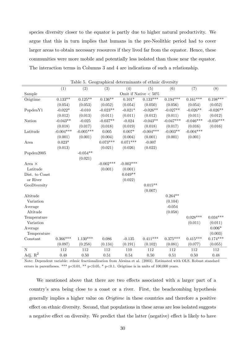
species diversity closer to the equator is partly due to higher natural productivity. We

argue that this in turn implies that humans in the pre-Neolithic period had to cover

larger areas to obtain necessary resources if they lived far from the equator. Hence, these

communities were more mobile and potentially less isolated than those near the equator.

The interaction terms in Columns 3 and 4 are indications of such a relationship.

Table 5. Geographical determinants of ethnic diversity(1) (2) (3) (4) (5) (6) (7) (8)

Sample Omit if Native < 50%Origtime 0.133** 0.125** 0.136** 0.101* 0.133*** 0.194*** 0.161*** 0.198***

(0.054) (0.053) (0.052) (0.054) (0.050) (0.056) (0.054) (0.052)PopdenY1 -0.022* -0.010 -0.023** -0.021* -0.026** -0.027** -0.026** -0.026**

(0.012) (0.013) (0.011) (0.011) (0.012) (0.011) (0.011) (0.012)Nation -0.043** -0.025 -0.037** -0.024 -0.043** -0.047*** -0.046*** -0.050***

(0.018) (0.017) (0.018) (0.019) (0.018) (0.017) (0.016) (0.016)Latitude -0.004*** -0.005*** 0.005 0.007* -0.004*** -0.003** -0.004***

(0.001) (0.001) (0.004) (0.004) (0.001) (0.001) (0.001)Area 0.023* 0.073*** 0.071*** -0.007

(0.013) (0.021) (0.026) (0.022)Popden2005 -0.054**

(0.021)Area � -0.002*** -0.002***Latitude (0.001) (0.001)Dist. to Coast 0.049**or River (0.022)GeoDiversity 0.015**

(0.007)Altitude 0.264**Variation (0.104)Average -0.054Altitude (0.058)Temperature 0.028*** 0.034***Variation (0.011) (0.011)Average 0.006*Temperature (0.003)Constant 0.366*** 1.130*** 0.086 -0.135 0.411*** 0.375*** 0.415*** 0.174***

(0.097) (0.258) (0.134) (0.191) (0.102) (0.081) (0.077) (0.055)N 112 112 112 110 112 112 112 112Adj. R2 0.48 0.50 0.51 0.54 0.50 0.51 0.50 0.48Note: Dependent variable: ethnic fractionalization from Alesina et al. (2003). Estimated with OLS. Robust standard

errors in parentheses. *** p<0.01, ** p<0.05, * p<0.1. Origtime is in units of 100,000 years.

We mentioned above that there are two e¤ects associated with a larger part of a

country�s area being close to a coast or a river. First, the beachcombing hypothesis

generally implies a higher value on Origtime in these countries and therefore a positive

e¤ect on ethnic diversity. Second, that populations in these areas are less isolated suggests

a negative e¤ect on diversity. We predict that the latter (negative) e¤ect is likely to have

30

dominated. When we include a measure of the mean distance to a coast or a river in

Column 4, we �nd that countries where the mean distance is shorter have a lower level

of ethnic fractionalization. Since we control for Latitude, Area, and their interaction, this

captures neither that populations in tropical countries choose to live in the cooler inland

areas, nor the e¤ect of populating a larger area (and hence having a longer mean distance

to a coast or a river) close to the equator.

The diversity of soil types (GeoDiversity), included in Column 5, is as mentioned

above a proxy for geographical friction. The within-country variations in temperature

and altitude are highly correlated in this sample (0.90), and including them both makes

both insigni�cant (not reported). Since the exact source of geographical friction and the

diversity in geographical living conditions are not in focus here, we are satis�ed with

including one of them in each regression, and hence leave the question of their relative

importance open. Latitude is highly correlated with Average Temperature (0.91), and the

overall results do not change when we replace Latitude with Average Temperature.

5.2 Robustness

In Tables 6 and 7, we investigate whether our results are sensitive to our choices of de-

pendent variable or indicator of duration of human settlements, or to the inclusion of

outliers. In Table 6, we have replaced ethnic fractionalization from Alesina et al. (2003)

with ethnic fractionalization from Fearon (2003) in Column 1, ethnolinguistic fractional-

ization (ELF ) in Column 2, and with the share of the population that do not belong to the

largest ethnic group (EthRest), also from Fearon (2003), in Column 3. While Origtime,

Nation, and Latitude remain signi�cant, PopdenY1 does not. We have already observed

that PopdenY1 is less robust than the other factors, and these results are in line with this

tendency.

In Section 4.1, we described two alternatives to Origtime: Fission and Migdist. The

�rst of these, Fission, is included in Columns 4 and 5 of Table 6. If Fission is used

instead of Origtime as our proxy for settlement duration, it is strongly signi�cant in

the predicted direction. The results in Column 5 show that Origtime does not merely

re�ect the variation in time since separation among the six world populations but also

the variation in the duration of settlements within them.

While Fission has fewer units of variation than Origtime since it is constructed based

31

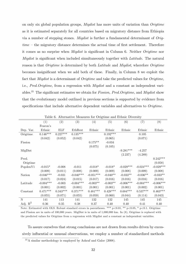
on only six global population groups, Migdist has more units of variation than Origtime

as it is estimated separately for all countries based on migratory distance from Ethiopia

via a number of stepping stones. Migdist is further a fundamental determinant of Orig-

time �the migratory distance determines the actual time of �rst settlement. Therefore

it comes as no surprise when Migdist is signi�cant in Column 6. Neither Origtime nor

Migdist is signi�cant when included simultaneously together with Latitude. The natural

reason is that Origtime is determined by both Latitude and Migdist, wherefore Origtime

becomes insigni�cant when we add both of these. Finally, in Column 8 we exploit the

fact thatMigdist is a determinant of Origtime and take the predicted values for Origtime,

i.e., Pred.Origtime, from a regression with Migdist and a constant as independent vari-

ables.35 The signi�cant estimates we obtain for Fission, Pred.Origtime, andMigdist show

that the evolutionary model outlined in previous sections is supported by evidence from

speci�cations that include alternative dependent variables and alternatives to Origtime.

Table 6. Alternative Measures for Origtime and Ethnic Diversity(1) (2) (3) (4) (5) (6) (7) (8)

Fearon�sDep. Var. Ethnic ELF EthRest Ethnic Ethnic Ethnic Ethnic EthnicOrigtime 0.146*** 0.227*** 0.135*** 0.192*** 0.105

(0.042) (0.052) (0.042) (0.065) (0.071)Fission 0.175** -0.034

(0.075) (0.105)MigDist -9.281*** -4.257

(2.237) (4.289)Pred. 0.242***Origtime (0.058)

PopdenY1 -0.015* -0.008 -0.011 -0.018* -0.018* -0.029*** -0.024*** -0.029***(0.009) (0.011) (0.008) (0.009) (0.009) (0.008) (0.009) (0.008)

Nation -0.046*** -0.031 -0.040*** -0.051*** -0.040** -0.033** -0.036** -0.033**(0.017) (0.024) (0.015) (0.017) (0.016) (0.016) (0.016) (0.016)

Latitude -0.004*** -0.003 -0.004*** -0.003** -0.003** -0.006*** -0.004*** -0.006***(0.001) (0.002) (0.001) (0.001) (0.001) (0.001) (0.002) (0.001)

Constant 0.471*** 0.343*** 0.371*** 0.481*** 0.428*** 0.684*** 0.537*** 0.463***(0.055) (0.071) (0.055) (0.059) (0.060) (0.044) (0.114) (0.043)

N 141 113 141 132 132 145 145 145Adj. R2 0.36 0.35 0.38 0.37 0.40 0.40 0.41 0.40Note: Estimated with OLS. Robust standard errors in parentheses. *** p<0.01, ** p<0.05, * p<0.1. Origtime

and Fission are in units of 100,000 years. MigDist is in units of 1,000,000 km. In (8), Origtime is replaced with

the predicted values for Origtime from a regression with Migdist and a constant as independent variables.

To assure ourselves that strong conclusions are not drawn from results driven by exces-

sively in�uential or unusual observations, we employ a number of standardized methods

35A similar methodology is employed by Ashraf and Galor (2008).

32

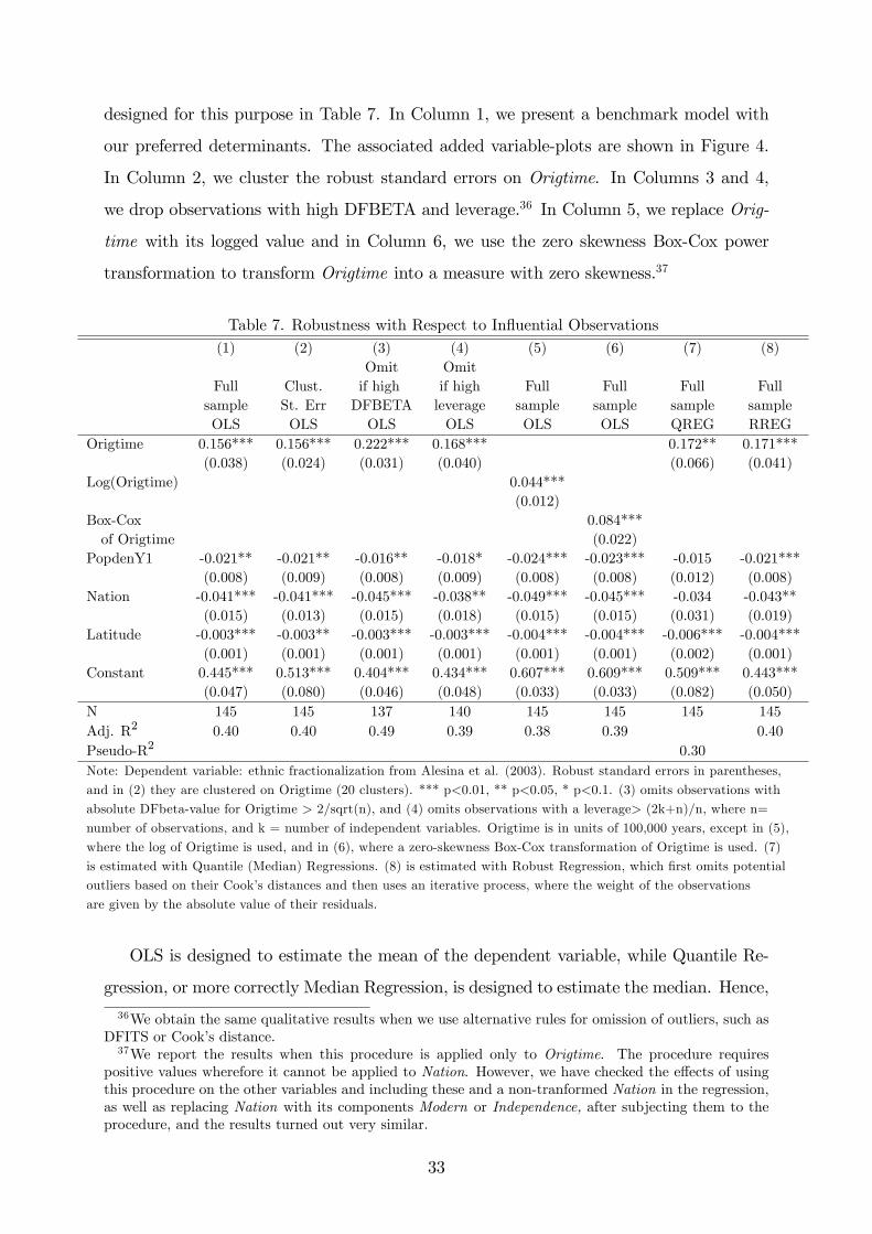
designed for this purpose in Table 7. In Column 1, we present a benchmark model with

our preferred determinants. The associated added variable-plots are shown in Figure 4.

In Column 2, we cluster the robust standard errors on Origtime. In Columns 3 and 4,

we drop observations with high DFBETA and leverage.36 In Column 5, we replace Orig-

time with its logged value and in Column 6, we use the zero skewness Box-Cox power

transformation to transform Origtime into a measure with zero skewness.37

Table 7. Robustness with Respect to In�uential Observations(1) (2) (3) (4) (5) (6) (7) (8)

Omit OmitFull Clust. if high if high Full Full Full Fullsample St. Err DFBETA leverage sample sample sample sampleOLS OLS OLS OLS OLS OLS QREG RREG

Origtime 0.156*** 0.156*** 0.222*** 0.168*** 0.172** 0.171***(0.038) (0.024) (0.031) (0.040) (0.066) (0.041)

Log(Origtime) 0.044***(0.012)

Box-Cox 0.084***of Origtime (0.022)

PopdenY1 -0.021** -0.021** -0.016** -0.018* -0.024*** -0.023*** -0.015 -0.021***(0.008) (0.009) (0.008) (0.009) (0.008) (0.008) (0.012) (0.008)

Nation -0.041*** -0.041*** -0.045*** -0.038** -0.049*** -0.045*** -0.034 -0.043**(0.015) (0.013) (0.015) (0.018) (0.015) (0.015) (0.031) (0.019)

Latitude -0.003*** -0.003** -0.003*** -0.003*** -0.004*** -0.004*** -0.006*** -0.004***(0.001) (0.001) (0.001) (0.001) (0.001) (0.001) (0.002) (0.001)

Constant 0.445*** 0.513*** 0.404*** 0.434*** 0.607*** 0.609*** 0.509*** 0.443***(0.047) (0.080) (0.046) (0.048) (0.033) (0.033) (0.082) (0.050)

N 145 145 137 140 145 145 145 145Adj. R2 0.40 0.40 0.49 0.39 0.38 0.39 0.40Pseudo-R2 0.30Note: Dependent variable: ethnic fractionalization from Alesina et al. (2003). Robust standard errors in parentheses,

and in (2) they are clustered on Origtime (20 clusters). *** p<0.01, ** p<0.05, * p<0.1. (3) omits observations with

absolute DFbeta-value for Origtime > 2/sqrt(n), and (4) omits observations with a leverage> (2k+n)/n, where n=

number of observations, and k = number of independent variables. Origtime is in units of 100,000 years, except in (5),

where the log of Origtime is used, and in (6), where a zero-skewness Box-Cox transformation of Origtime is used. (7)

is estimated with Quantile (Median) Regressions. (8) is estimated with Robust Regression, which �rst omits potential

outliers based on their Cook�s distances and then uses an iterative process, where the weight of the observations

are given by the absolute value of their residuals.

OLS is designed to estimate the mean of the dependent variable, while Quantile Re-

gression, or more correctly Median Regression, is designed to estimate the median. Hence,

36We obtain the same qualitative results when we use alternative rules for omission of outliers, such asDFITS or Cook�s distance.37We report the results when this procedure is applied only to Origtime. The procedure requires

positive values wherefore it cannot be applied to Nation. However, we have checked the e¤ects of usingthis procedure on the other variables and including these and a non-tranformed Nation in the regression,as well as replacing Nation with its components Modern or Independence, after subjecting them to theprocedure, and the results turned out very similar.

33

the estimates in Column 7 are less sensitive to extreme outliers. It has been noted that

also Quantile Regressions are sensitive to observations with high leverage, and in results

not shown estimated the same speci�cation as in Column 7 on a sample where observa-

tions with high leverage were omitted, and the results were similar. Robust Regressions

is another method designed to ensure that the results are not driven by outliers. We

use this method for the speci�cation in Column 8. Summing up Tables 6 and 7, we �nd

that the results for the duration of human settlements are not driven by our choice of

dependent variable, by our construction of Origtime, or by the inclusion of in�uential or

unusual observations.

6 Concluding remarks

Ethnic diversity has caught the attention of many a social scientist struggling to under-

stand problems such as low provision of public goods, low quality governance, persistent

economic backwardness, and civil wars. The general approach in much of this research

has been to treat ethnic diversity as an exogenous factor, and few have explicitly referred

to the evolutionary or constructivist discourses on the origins of ethnicity.

In this paper we have brie�y portrayed this literature and synthesized it with �ndings

from ecology, anthropology, and genetics, showing how geographical and ecological fac-

tors in�uence human ethnic diversity. We have constructed a measure for the historical

duration of human settlements in an area and a theoretical model explaining how such

measures should be related to ethnic diversity. The empirical analysis clearly indicates

that ethnic diversity is higher in countries where humans settled earlier and where geo-

graphical conditions have enabled and encouraged isolation, and lower in countries where

early civilization proved more successful and where the state was stronger during the

modern nation-state era.

Our results have important speci�c implications for how social scientists investigate

the e¤ect of ethnic diversity on economic and political outcomes. For instance, an often

employed method for assessing the e¤ect of ethnic diversity on economic and political

performance has been to include a measure of ethnic fractionalization as one of many

potential regressors. Since a stronger state in the nation-state era is associated with a

lower degree of ethnic diversity, and since there is a positive correlation between indicators

34

of this strength and many indicators of economic and political performance, the negative

coe¢ cient on ethnicity obtained in these regressions could re�ect an omitted variable

bias �they may be mere statistical artefacts created by the omission of long-term state

strength from the regression.

On a more general level, a reasonable projection of our results is that the world is

going to experience a continuing decrease in levels of ethnic diversity in the centuries

ahead. We believe that the economic and political impact of this process is a promising

area for future research and that a serious understanding of ethnic diversity requires a

synthesis of evolutionary and constructivist arguments, as proposed in this paper.

35

ReferencesAkerlof, G.A. (1997) �Social Distance and Social Decisions�Econometrica, 65(5):1005-27.

Akerlof, G.A. and R.E. Kranton (2000) �Economics and Identity� Quarterly Journal ofEconomics, 65(3):715-53.

Alesina, A., A. Devleeschauwer, W. Easterly, S. Kurlat, and R. Wacziarg (2003) �Fraction-alization�Journal of Economic Growth, 8:155-94.


Alesina, A. and E. Spolaore (1997) �On the Number and Size of Nations�Quarterly Journalof Economics, 112(4):1027-56.

Alesina, A. and E. Spolaore (2003) The Size of Nations, Boston: MIT Press.

Alesina, A. and R. Wacziarg (1998) �Openness, Country Size, and Government�Journal ofPublic Economics, 69:305-21.

Anderson, B. (1983) Imagined Communities: Re�ections on the origin and spread of nation-alism, London: Verso.

Ashraf, Q. and O. Galor (2008) �Human Genetic Diversity and Comparative EconomicDevelopment�mimeo, Brown University.

Ashraf, Q. and O. Galor (2007) �Cultural Assimilation, Cultural Di¤usion, and the Originof the Wealth of Nations�mimeo, Brown University.

Bates, R. (2006) �Ethnicity� in The Elgar Companion to Development Studies (ed. D.A.Clark), 167-73, Cheltenham: Edward Elgar.

van den Berghe, P.L. (1981) The Ethnic Phenomenon, Westport: Praeger.

van den Berghe, P.L. (1995) �Does Race Matter?�Nations and Nationalism, 1(3):357-68.

Bockstette, V., A. Chanda, and L. Putterman (2002) �States and Markets: The Advantageof and Early Start�Journal of Economic Growth, 7:347-69.

Bradshaw Foundation (2007), available online at http://www.bradshawfoundation.com/stephenoppenheimer/.

Caselli, F. and W.J. Coleman II. (2006) �On the Theory of Ethnic Con�ict�mimeo, LondonSchool of Economics.

Cashdan, E. (2001) �Ethnic diversity and its environmental determinants: E¤ects of climate,pathogens, and habitat diversity�American Anthropologist, 103:968-91.

Cavalli-Sforza, L., A. Piazza, P. Menozzi, and J. Mountain (1988) �Reconstruction of humanevolution: Bringing together genetic, archaeological, and linguistic data�Proceedings ofthe National Academy of Science, 85:6002-6.

Cavalli-Sforza, L., P. Menozzi, and A. Piazza (1994) The History and Geography of HumanGenes, Princeton: Princeton University Press.

Cavalli-Sforza, L. and F. Cavalli-Sforza (1995) The Great Human Diasporas: The History ofDiversity and Evolution, Cambridge: Perseus Books.

Cepii, �Centre d�Etude Prospective et d�Informations Internationales,� available online athttp://www.cepii.fr.

Chanda, A. and L. Putterman (2007) �Early Starts, Reversals and Catch-up in the Processof Economic Development�Scandinavian Journal of Economics, 109(2):387-413.

Chaplin, G. (2004) �Geographic Distribution of Environmental Factors In�uencing HumanSkin Coloration�American Journal of Physical Anthropology, 125:292-302.

36

CIA, World Factbook, available online at https://www.cia.gov/cia/publications/factbook/index.html.

CID (2001) �GEOGRAPHY DATASETS,�Center for International Development, HarvardUniversity, available online at http://www.cid.harvard.edu.

Cohen, V.G. (1977) The Food Crisis in Prehistory: Overpopulation and the Origins of Agri-culture, New Haven: Yale University Press.

Collard, I. and R.A. Foley (2002) �Latitudinal patterns and environmental determinants ofrecent human cultural diversity: do humans follow biogeographical rules?�EvolutionaryEcology Research, 4:371-83.

Collier, P. (2000) �Ethnicity, Politics and Economic Performance�Economics and Politics,12(3):225-45.

Collier, P. (2001) �Implications of Ethnic Diversity�Economic Policy, 16(32):128-66.

Collier, P. and A. Hoe er (2004) �Greed and Grievance in civil war� Oxford EconomicPapers, 56:563-95.

COW, Correlates of War Project, available online at http://www.correlatesofwar.org/.

Dawkins, R. (1976) The Sel�sh Gene, Oxford: Oxford University Press.

Dawkins, R. (2006) The God Delusion, New York: Transworld.

Diamond, J. (1997) Guns, Germs and Steel: The Fates of Human Societies, New York:W.W. Norton.

Dunn, M., A. Terrill, G. Reesink, R. Foley, and S. Levinson (2005) �Structural Phylogeneticsand the Reconstruction of Ancient Language History�Science, 309(5743):2072-5.

Easterly, W. (2001) �Can institutions resolve ethnic con�ict?�Economic Development andCultural Change, 49(4):687-706.


Encyclopedia Britannica (2007), available online at http://www.britannica.com.

Fearon, J.D. ( 2003) �Ethnic and Cultural Diversity by Country� Journal of EconomicGrowth, 8:195-222.

Fincher, C.L., R. Thornhill, D.R. Murray, and M. Schaller (2008) �Pathogen PrevalencePredicts Human Cross-Cultural Variability in Individualism/Collectivism�Proceedingsof the Royal Society B, 275:1279-85.

G-Econ (2006), available online at http://gecon.yale.edu/.

Galor, O. and O. Moav (2002) �Natural Selection and The Origin of Economic Growth�Quarterly Journal of Economics, 117(4):1133-91.


Herbst, J. (2000) States and Power in Africa: Comparative Lessons in Authority and Control,Princeton: Princeton University Press.

Jablonski, N.G. (2004) �The Evolution of Human Skin and Skin Color�Annual Review ofAntropology, 33:585-623.

Jones, E. (1981) The European Miracle: Environments, Economies, and Geopolitics in Eu-rope and Asia, Cambridge: Cambridge University Press.

Jones, D. (2000) �Group Nepotism and Human Kinship�Current Anthropology 41(5):779-809.

Hobsbawm, E.J. and T. Ranger (1983) The Invention of Tradition, Cambridge: CambridgeUniversity Press.

37

Ingman, M., H. Kaessman, S. Pääbo, and U. Gyllensten (2000) �Mitochondrial GenomeVariation and the Origin of Modern Humans�Nature, 408:708-13.

Kimenyi, M.S. (2006) �Ethnicity, Governance and the Provision of Public Goods�Journalof African Economies, 15:62-99.


Leeson, P.T. (2005) �Endogenizing fractionalization� Journal of Institutional Economics1(1):75�98.

Liu, H., F. Prugnolle, A. Manica, and F. Balloux (2006) �A Geographically Explicit GeneticModel of Worldwide Human-Settlement History�American Journal of Human Genetics,79:230-37.

Macaulay, V., C. Hill, A. Achilli, C. Rengo, D. Clarke, W. Meehan, J. Blackburn, O. Semino,R. Scozzari, F. Cruciani, A. Taha, N.K. Shaari, J.M. Raja, P. Ismail, Z. Zainuddin, W.Goodwin, D. Bulbeck, H-J. Bandelt, S. Oppenheimer, A. Torroni, and M. Richards(2005) �Single, Rapid Coastal Settlement of Asia Revealed by Analysis of CompleteMitochondrial Genomes�, Science, 308(5724):1034-6.

Mace, R. and M. Pagel (1995) �A latitudinal gradient in the density of human languages inNorth America�Proceedings of the Royal Society of London, B-Series, 261:117-21.

McDougall, I., F. Brown, and J. Fleagle (2005) �Stratigraphic Placement and Age of ModernHumans from Kibish, Ethiopia�Nature, 433:733-6.

Michalopoulos, S. (2008) �Ethnolinguistic Diversity: Origins and Implications�mimeo, TuftsUniversity.

Miguel, E. (2004) �Tribe or Nation? Nation Building and Public Goods in Kenya versusTanzania�World Politics, 56(3):327-62.

Olsson, O. (2001) �The Rise of Neolithic Agriculture�mimeo, University of Gothenburg.

Olsson, O. and D.A. Hibbs (2005) �Biogeography and Long-Run Economic Development�European Economic Review, 49(4):909-38.

Olsson, O. (2007) �On the Institutional Legacy of Mercantilist and Imperialist Colonialism�Working Papers in Economics No. 247, University of Gothenburg.


Osterhammel, J. (2005) Colonialism, Princeton: Markus Wiener Pub.

Pagel, M. and R. Mace (2004) �The cultural wealth of nations�Nature, 428:275-8.

Putterman, L. (2008a) �Agriculture, Di¤usion, and Development: Ripple E¤ects of theNeolithic Revolution�Economica, 75(300):729-48.

Putterman, L. (2008b), available online at http://www.econ.brown.edu/fac/Louis_Putterman.

Putterman, L. and D. Weil (2008) �Post-1500 Population Flows and the Long-Run Deter-minants of Economic Growth and Inequality�mimeo, Brown University.

Ramachandran, S., O. Deshpande, C.C. Roseman, N.A. Rosenberg, M.W. Feldman, and L.Cavalli-Sforza (2005) �Support for the relationship of genetic and geographic distance inhuman populations for a serial founder e¤ect origininating in Africa�Proceedings of theNational Academy of Science, 102(44):15942-7.

Sahlins, M. (1972) Stone Age Economics, New York: Aldine de Gruyter.

Shils, E. (1957) �Primordial, Personal, Sacred, and Civil Ties�British Journal of Sociology,7:113-45.

38

Smith, B.D. (1998) The Emergence of Agriculture, New York: Scienti�cAmerican Library.

Smith, A.D. (1986) The Ethnic Origin of Nations, Oxford: Basil Blackwell.

Spolaore, E. and R. Wacziarg (2006) �The Di¤usion of Development�NBER Working Paper12153.


Tishko¤, S. and B. Verelli (2003) �Patterns of Human Genetic Diversity: Implications forHuman Evolutionary History and Disease� Annual Review of Genomics and HumanGenetics, 4:293-340.

WDI Online, available online at http://www.worldbank.org/.

Worldmapper (2006), available online at http://www.worldmapper.org.

39

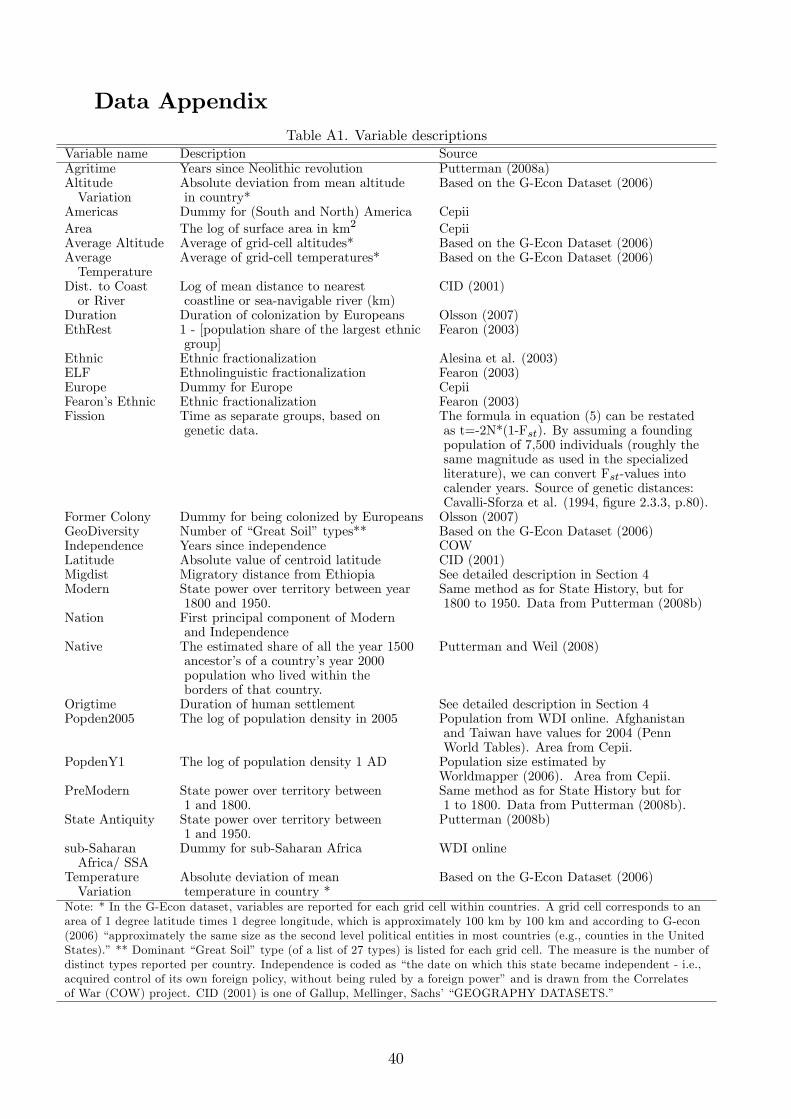
Data AppendixTable A1. Variable descriptions

Variable name Description SourceAgritime Years since Neolithic revolution Putterman (2008a)Altitude Absolute deviation from mean altitude Based on the G-Econ Dataset (2006)Variation in country*

Americas Dummy for (South and North) America CepiiArea The log of surface area in km2 CepiiAverage Altitude Average of grid-cell altitudes* Based on the G-Econ Dataset (2006)Average Average of grid-cell temperatures* Based on the G-Econ Dataset (2006)Temperature

Dist. to Coast Log of mean distance to nearest CID (2001)or River coastline or sea-navigable river (km)

Duration Duration of colonization by Europeans Olsson (2007)EthRest 1 - [population share of the largest ethnic Fearon (2003)

group]Ethnic Ethnic fractionalization Alesina et al. (2003)ELF Ethnolinguistic fractionalization Fearon (2003)Europe Dummy for Europe CepiiFearon�s Ethnic Ethnic fractionalization Fearon (2003)Fission Time as separate groups, based on The formula in equation (5) can be restated

genetic data. as t=-2N*(1-Fst). By assuming a foundingpopulation of 7,500 individuals (roughly thesame magnitude as used in the specializedliterature), we can convert Fst-values intocalender years. Source of genetic distances:Cavalli-Sforza et al. (1994, �gure 2.3.3, p.80).

Former Colony Dummy for being colonized by Europeans Olsson (2007)GeoDiversity Number of �Great Soil�types** Based on the G-Econ Dataset (2006)Independence Years since independence COWLatitude Absolute value of centroid latitude CID (2001)Migdist Migratory distance from Ethiopia See detailed description in Section 4Modern State power over territory between year Same method as for State History, but for

1800 and 1950. 1800 to 1950. Data from Putterman (2008b)Nation First principal component of Modern

and IndependenceNative The estimated share of all the year 1500 Putterman and Weil (2008)

ancestor�s of a country�s year 2000population who lived within theborders of that country.

Origtime Duration of human settlement See detailed description in Section 4Popden2005 The log of population density in 2005 Population from WDI online. Afghanistan

and Taiwan have values for 2004 (PennWorld Tables). Area from Cepii.

PopdenY1 The log of population density 1 AD Population size estimated byWorldmapper (2006). Area from Cepii.

PreModern State power over territory between Same method as for State History but for1 and 1800. 1 to 1800. Data from Putterman (2008b).

State Antiquity State power over territory between Putterman (2008b)1 and 1950.

sub-Saharan Dummy for sub-Saharan Africa WDI onlineAfrica/ SSA

Temperature Absolute deviation of mean Based on the G-Econ Dataset (2006)Variation temperature in country *

Note: * In the G-Econ dataset, variables are reported for each grid cell within countries. A grid cell corresponds to anarea of 1 degree latitude times 1 degree longitude, which is approximately 100 km by 100 km and according to G-econ(2006) �approximately the same size as the second level political entities in most countries (e.g., counties in the UnitedStates).�** Dominant �Great Soil�type (of a list of 27 types) is listed for each grid cell. The measure is the number ofdistinct types reported per country. Independence is coded as �the date on which this state became independent - i.e.,acquired control of its own foreign policy, without being ruled by a foreign power�and is drawn from the Correlatesof War (COW) project. CID (2001) is one of Gallup, Mellinger, Sachs��GEOGRAPHY DATASETS.�

40

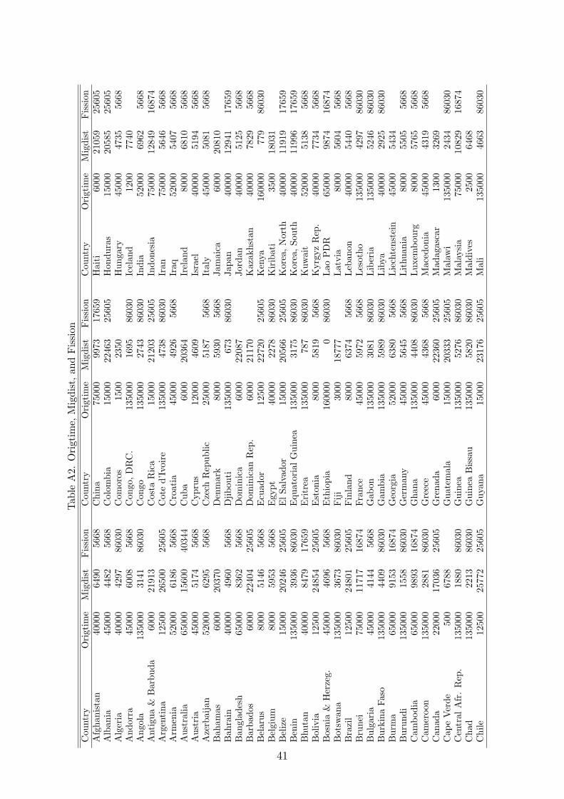
TableA2.Origtime,Migdist,andFission

Country

Origtime

Migdist

Fission

Country

Origtime

Migdist

Fission

Country

Origtime

Migdist

Fission

Afghanistan

40000

6490

5668

China

75000

9973

17659

Haiti

6000

21059

25605

Albania

45000

4482

5668

Colombia

15000

22463

25605

Honduras

15000

20585

25605

Algeria

40000

4297

86030

Comoros

1500

2350

Hungary

45000

4735

5668

Andorra

45000

6008

5668

Congo,DRC.

135000

1695

86030

Iceland

1200

7740

Angola

135000

3141

86030

Congo

135000

2743

86030

India

52000

6962

5668

Antigua&Barbuda

6000

21913

CostaRica

15000

21203

25605

Indonesia

75000

12849

16874

Argentina

12500

26500

25605

Coted�Ivoire

135000

4738

86030

Iran

75000

5646

5668

Armenia

52000

6186

5668

Croatia

45000

4926

5668

Iraq

52000

5407

5668

Australia

65000

15600

40344

Cuba

6000

20364

Ireland

8000

6810

5668

Austria

45000

5174

5668

Cyprus

12000

4609

Israel

40000

5194

5668

Azerbaijan

52000

6295

5668

CzechRepublic

25000

5187

5668

Italy

45000

5081

5668

Bahamas

6000

20370

Denmark

8000

5930

5668

Jamaica

6000

20810

Bahrain

40000

4960

5668

Djibouti

135000

673

86030

Japan

40000

12941

17659

Bangladesh

65000

8362

5668

Dominica

6000

22087

Jordan

40000

5125

5668

Barbados

6000

22404

25605

DominicanRep.

6000

21170

Kazakhstan

40000

7829

5668

Belarus

8000

5146

5668

Ecuador

12500

22720

25605

Kenya

160000

779

86030

Belgium

8000

5953

5668

Egypt

40000

2278

86030

Kiribati

3500

18031

Belize

15000

20246

25605

ElSalvador

15000

20566

25605

Korea,North

40000

11919

17659

Benin

135000

3936

86030

EquatorialGuinea

135000

3175

86030

Korea,South

40000

11996

17659

Bhutan

40000

8479

17659

Eritrea

135000

787

86030

Kuwait

52000

5138

5668

Bolivia

12500

24854

25605

Estonia

8000

5819

5668

KyrgyzRep.

40000

7734

5668

Bosnia&Herzeg.

45000

4696

5668

Ethiopia

160000

086030

LaoPDR

65000

9874

16874

Botswana

135000

3673

86030

Fiji

3000

18777

Latvia

8000

5604

5668

Brazil

12500

24801

25605

Finland

8000

6374

5668

Lebanon

40000

5440

5668

Brunei

75000

11717

16874

France

45000

5972

5668

Lesotho

135000

4297

86030

Bulgaria

45000

4144

5668

Gabon

135000

3081

86030

Liberia

135000

5246

86030

BurkinaFaso

135000

4409

86030

Gambia

135000

5989

86030

Libya

40000

2925

86030

Burma

65000

9153

16874

Georgia

52000

6380

5668

Liechtenstein

45000

5434

Burundi

135000

1558

86030

Germany

45000

5645

5668

Lithuania

8000

5505

5668

Cambodia

65000

9893

16874

Ghana

135000

4408

86030

Luxembourg

8000

5765

5668

Cameroon

135000

2881

86030

Greece

45000

4368

5668

Macedonia

45000

4319

5668

Canada

22000

17036

25605

Grenada

6000

22360

25605

Madagascar

1300

3269

CapeVerde

500

6788

Guatemala

15000

20333

25605

Malawi

135000

2434

86030

CentralAfr.Rep.

135000

1880

86030

Guinea

135000

5276

86030

Malaysia

75000

10829

16874

Chad

135000

2213

86030

GuineaBissau

135000

5820

86030

Maldives

2500

6468

Chile

12500

25772

25605

Guyana

15000

23176

25605

Mali

135000

4663

86030

41

TableA2.Origtime,Migdist,andFission,continued

Country

Origtime

Migdist

Fission

Country

Origtime

Migdist

Fission

Country

Origtime

Migdist

Fission

Malta

5000

5113

St.Vincent/Grenad.

6000

22289

UnitedArabEm.

75000

5022

5668

MarshallIslands

3500

17343

Samoa

3000

19970

UnitedKingdom

8000

6460

5668

Mauritania

135000

5542

86030

SanMarino

45000

5126

5668

UnitedStates

22000

17909

25605

Mauritius

500

3807

SaoTome&Principe

500

3525

Uruguay

12500

26836

25605

Mexico

15000

19011

25605

SaudiArabia

40000

4589

5668

Uzbekistan

40000

7039

5668

Micronesia(Fed.St.)

3500

16312

Senegal

135000

5711

86030

Vanuatu

3000

17898

Moldova

25000

4483

5668

Serbia&Montenegro

45000

4474

5668

Venezuela

15000

22459

25605

Monaco

45000

5527

Seychelles

200

2411

Vietnam

75000

9986

16874

Mongolia

40000

10166

17659

SierraLeone

135000

5450

86030

Yemen

85000

3896

5668

Morocco

40000

5180

86030

Singapore

75000

9887

16874

Zambia

135000

2709

86030

Mozambique

135000

2941

86030

SlovakRepublic

25000

4895

5668

Zimbabwe

135000

3238

86030

Namibia

135000

4051

86030

Slovenia

45000

4996

5668

Nauru

3000

17413

SolomonIslands

35000

16785

Nepal

40000

7869

17659

Somalia

135000

1230

86030

Netherlands

8000

5922

5668

SouthAfrica

135000

4385

86030

NewZealand

1200

19535

Spain

40000

6506

5668

Nicaragua

15000

20859

25605

SriLanka

52000

7301

5668

Niger

135000

3382

86030

Sudan

135000

1170

86030

Nigeria

135000

3305

86030

Suriname

15000

23459

25605

Norway

8000

6439

5668

Swaziland

135000

3905

86030

Oman

75000

5059

5668

Sweden

8000

6305

5668

Pakistan

52000

6694

5668

Switzerland

45000

5539

5668

Palau

4500

13708

Syria

40000

5562

5668

Panama

15000

21523

25605

Taiwan

75000

11511

PapuaNewGuinea

65000

15462

40344

Tajikistan

40000

7328

5668

Paraguay

12500

25814

25605

Tanzania

135000

1594

86030

Peru

12500

23578

25605

Thailand

65000

9345

16874

Philippines

17000

12308

5668

Togo

135000

4059

86030

Poland

8000

5178

5668

Tonga

3000

19851

Portugal

40000

6852

5668

Trinidad&Tobago

15000

22504

Qatar

40000

4958

5668

Tunisia

40000

4149

86030

Romania

45000

4417

5668

Turkey

52000

4447

5668

Russia

25000

10274

5668

Turkmenistan

40000

6736

5668

Rwanda

135000

1424

86030

Tuvalu

700

18800

St.Kitts&Nevis

6000

21826

Uganda

135000

1025

86030

SaintLucia

6000

22237

Ukraine

25000

4754

5668

42

Figures

Figure 1. The human genealogy

Notes: The figure shows the genetic distance (using mitochondrial DNA) between ethnic

groups across the world, based on a sample of 53 individuals. Information such as “138k”

refers to the approximate date when genetic branches split up, whereas for instance “L1k” is

the name of a particular genetic branch. The source is Oppenheimer (2003), based on Ingman

et al. (2000).

43

Figure 2. Evolutionary, constructivist, and geographical influences on ethnic

diversity over time.

Figure 3a. Geographical niches within an ethnic group (q=3).

0 s/2

p

Core niche c

(mi(t)=1)

z

Peripheral

niche (mi(t)>1)

Peripheral

niche (mi(t)>1)

qs /2 qs / s

Original

settlement

Ethnic

diversity

Sedentary

agriculture

Statehood

Western

colonialism

Geography

(topography, bio-

geography, climate)

Random shocks

(natural disasters, climate change, migrations)

time

44

Figure 3b. Effective level of public goods supply at different locations (q=3).

Figure 4. Added variable plots for specification 1 in Table 7.

Note: The observations are represented by their respective three-letter identification code,

following the World Bank classification.

SYC

MDG

CPV

GUY

PAN

FJI

ECU

GRD

MUSCOLTTO

BRB

JAMVENBRANIC

CUB

CRI

DOM

PER

PHL

NZL

HND

BOL

SLV

GTM

HTIPRY

MEX

URY

CYP

ARG

PNG

CHL

SGP

LKA

POL

BLR

MYSDZAIRL

LTU

TKM

JOR

LAO

IDN

EST

LVA

EGY

KHM

ISRMMR

USA

ISL

BEL

TJK

MDA

MARSYR

IND

FIN

UKR

THA

KGZ

SVK

AFG

VNM

CZE

NLD

UZB

NPL

MNG

NOR

KAZ

TUN

PAKCAN

ROK

MKD

ARM

AUS

BIH

SWE

AZE

ALB

BGD

SVN

GBR

GEO

HRVROM

JPN

BGR

HUNGRC

DNK

YUG

ESP

TWNITAAUT

RUS

PRT

TUR

DEU

CHE

GAB

CAFCOG

IRN

FRA

UGA

SLE

LBR

TGO

CMRZAR

GHA

CIVTCD

GIN

SOM

CHN

BEN

NGA

BDI

AGOGMB

SENBFA

RWA

MLI

MRT

MOZKEN

NER

MWISDNZMB

ZWEBWA

SWZ

ZAF

LSO

ETH

-.4

-.2

0.2

.4

e(

Eth

nic

| X

)

-1 -.5 0 .5 1e( Origtime | X )

coef = .15590389, (robust) se = .03820217, t = 4.08

NZL

MDG

PAN

CAN

SGPVNM

THA

LAOMMRFINARGMRT

BWA

USA

URYMNGNER

PRY

TCDBRA

ISL

AUS

MLI

NORSWE

KAZ

CHL

RUSZAF

TKMMOZ

BOL

VEN

HND

LBR

CRI

COLCIV

DOMNICGINCPV

ZWE

CMR

SEN

KHM

MYS

BFABEN

KGZECU

SWZ

POL

TJK

GBRTGOGHAUZB

EST

LSO

GUYGMB

PNG

DZA

CUBSLE

LVA

JORGTMMEX

DNKKEN

NGA

GAB

SOM

MWI

IRL

MARCAFETHZMB

BLRFJICOG

LTUAGO

NLD

PERUGA

AFG

HUNAZE

ROM

IRN

SDN

SLV

SYR

PRT

ARM

GEO

TTO

BGR

AUT

UKR

HRV

CHEBEL

ZARBIH

FRADEUSVK

MKD

TUNSYC

YUG

HTI

SVN

CZE

EGY

ISR

IDNMUS

CHNCYP

TUR

ESP

ALB

JPN

MDA

JAM

NPLPAK

GRC

ROK

TWNPHLITALKA

IND

GRD

BDIRWA

BGD

BRB

-.5

0.5

e(

Eth

nic

| X

)

-10 -5 0 5e( PopdenY1 | X )

coef = -.02116671, (robust) se = .008295, t = -2.55

TKM

FJI

PNG

BLR

ARM

UKRMDAESTKGZ

LTU

SVKSVNPOL

BIHKAZMKD

CYP

NZL

CZEGEOTJKCAF

AZE

LVA

MUS

IRLBRB

JAMKEN

GRDISRCPV

JOR

UZBSLE

SYC

IND

SYRTTO

MNG

GUY

DZA

HRV

TCD

BGD

ROMLKAALB

TGOGAB

PHLHUNISLMMRFIN

CUB

PAK

LAONOR

ZWE

MDG

AGO

LSO

IDN

MYS

GMB

AFG

MOZSENGIN

BWA

MRT

SGPKHM

EGY

ROK

GHA

SDNMARCOG

MLI

ZAFBGR

SWZ

NGABEN

LBRZMB

MWI

VNM

CAN

BFA

TWN

ZAR

BDI

NIC

SOMCIV

NER

CMR

YUGUGA

BEL

AUT

USA

PANDOM

GRC

TUN

URYARGCHLITA

HND

AUS

RWA

MEX

SLV

GTM

BOL

CRI

PER

DEU

HTI

VEN

ECU

PRY

BRACOL

NPL

NLDSWE

ETHTHA

JPN

RUS

ESP

TUR

IRN

CHN

CHE

GBR

PRT

DNKFRA

-.6

-.4

-.2

0.2

.4

e(

Eth

nic

| X

)

-2 -1 0 1 2 3e( Nation | X )

coef = -.04112326, (robust) se = .01545273, t = -2.66

ECU

SYC

COL

PER

VENGUY

BRB

GRD

CRIPHLSLV

TTOIDNBRA

LKA

HTI

GTM

NIC

HND

MYS

RWA

BOL

JAMPANDOMCPV

MUS

BDI

FJI

PNG

UGAMEXCUB

SGP

COGZAR

KHM

PRY

GAB

NPL

SOMTHAIND

CMR

BGD

MDG

EGY

KENETH

LBR

TWN

CIV

GHA

NGACAFBEN

TGO

SLE

PRT

JPN

ZMBAGOSDNMWIGINBFA

PAK

TUN

DZA

VNM

URY

CYP

IRN

MAR

LAOCHL

ESPGMB

ISR

AUS

TUR

ROK

CHN

AFG

JOR

SEN

MMRARGFRAGRC

SYR

ITA

MOZNER

CHE

MLI

TCD

ZWE

GBRDNK

ALBNLD

YUGBEL

BGRTJK

MRT

MKD

SWZ

UZB

AZEARM

AUT

BWA

USA

MDA

HRVGEO

KGZ

DEU

BIH

ROMTKMSVKCZE

LSO

SVNHUN

UKRZAF

NZLIRLPOL

BLRLTU

MNG

LVA

KAZ

SWE

RUS

EST

ISLFIN

CAN

NOR

-.6

-.4

-.2

0.2

.4

e(

Eth

nic

| X

)

-40 -20 0 20 40e( Latitude | X )

coef = -.0034675, (robust) se = .00109402, t = -3.17

0 s/2

gi

z

g

slope: g

slope: tmg i

qs /

qs /2

s

tP

gs

2

tP

gs

2

45

The Causal E¤ects of Ethnic Diversity:An Instrumental Variables Approach

Pelle Ahlerup�


September 2009

Abstract

Ethnic diversity is endogenous to economic development in the long run. Yet the

standard approach in economic research is to treat ethnic diversity as an exogenous

factor. By identifying instruments for ethnic diversity, we correct this misspeci�ca-

tion and establish that ethnic diversity has an exogenous in�uence on income levels,

economic growth, corruption, and provision of public goods. Earlier results based

on OLS estimations may have underestimated the negative e¤ects of high levels of

ethnic diversity.

Keywords: economic development, ethnic diversity, instrumental variables,

property rights.

JEL classi�cation: O11, O43, P51

1 Introduction

High levels of ethnic diversity have been linked to various poor economic and political

outcomes, e.g., lower income levels and lower economic growth (Easterly and Levine

1997, Alesina et al. 2003, Alesina and La Ferrara 2005) and more corruption and a lower

provision of public goods (Mauro 1995, Easterly and Levine 1997, La Porta et al. 1999,

Alesina et al. 2003).1 The standard approach in this literature has been to treat ethnic

diversity as if it were exogenous to economic development. However, we argue that this

is a misspeci�cation.

Two recent papers demonstrate that ethnic diversity is determined by historical forces

and geographical factors. Ahlerup and Olsson (2007) show that the levels of ethnic di-

versity in di¤erent countries follow a number of predictable patterns. Ethnic diversity

�Dept. of Economics, University of Gothenburg, Box 640, 405 30 Gothenburg, Sweden. Email:[email protected]. The paper has bene�ted greatly from discussions with Ola Olsson, Carl-Johan Dalgaard, Sven Tengstam, Erik Linquist, participants at CSAE 2009, and colleagues at the Uni-versity of Gothenburg.

1A nice overview of this literature can be found in Alesina and La Ferrara (2005).

1

is higher in countries with a longer duration of human settlement, and in countries that

have a naturally fragmented geography, that lie closer to the equator, and that have had

low levels of territorial state capacity during the modern era. The prehistoric formation

of ethnic groups is modeled as depending on the groups�ability to provide public goods

to group members.

The duration of uninterrupted human settlements a¤ects ethnic diversity because the

formation of new ethnic groups takes a considerable amount of time. The fragmentation

process will therefore have come further in areas where humans have lived for a longer

time.2 Indicators for geographical fragmentation capture the fact that a fragmented ge-

ography makes it harder for the groups to provide public goods (or broadcast power

and control) over longer geographical distances. This reduces interaction and allows new

ethnic identities to form over time.

The endogenous nature of ethnic diversity is also explored by Michalopoulos (2008),

who models ethnic diversity as originating in di¤erences in land quality. These di¤erences

generate localized human capital which reduces mobility, and allows local ethnicities to

form.3

Historical accounts of how populations in more developed countries have become more

homogenous in the last centuries, through a combination of deliberate homogenizing ef-

forts and endogenous processes, can be found in Anderson (1983), Gellner (1983), and

Tilly (1992). These processes are discussed in more detail below.

Ethnic diversity is thus endogenous to economic development in the long run. Yet,

although this notion is widespread among economists who study the e¤ects of ethnic diver-

sity, ethnic diversity is generally treated as an exogenous explanatory factor in empirical

analyses. In�uential articles in this tradition include Easterly and Levine (1997) and La

Porta et al. (1999). Only a few studies question the exogeneity of ethnic diversity. Mauro

(1995) discusses how factors omitted from his estimation may have a¤ected both colonial

history and ethnolinguistic fractionalization, and Acemoglu et al. (2001), Fearon (2003),

and Alesina and La Ferrara (2005) argue that contemporary levels of ethnic diversity are

partly determined by long-run economic development.4

Let us brie�y discuss how previous studies on ethnic diversity and long-run devel-

opment may have obtained biased estimates due to omitted variables, simultaneity, or

measurement error.

When two true determinants are correlated with each other but one of them is omitted,

the estimate of the included variable can be biased. The direction of the bias will depend

2The e¤ect of the duration of human settlements is demonstrated to be robust to a wide range ofspeci�cations and the omission of potential outliers, among both former colonies and countries nevercolonized by Europeans, and when global migration �ows since 1500 AD are taken into account. Thee¤ect is not driven by the experiences of countries in sub-Saharan Africa or the Americas.

3In his empirical analysis, Michalopoulos (2008) �nds higher ethnolinguistic fractionalization in coun-tries with a greater range in the quality of land.

4For a model that endogenizes ethnicity, see Caselli and Coleman (2006).

2

on the sign of the correlation, and on whether the omitted variable has a positive or

negative e¤ect on the dependent variable.

Consider two hypothetical cases that can result in biased estimates. First, suppose

that some societies have a culture that is more open to the in�ow of new ideas and

people. Over time, these societies will both be economically more successful and have

more heterogenous populations. If the heterogeneity is included in an analysis of long-run

development but the cultural openness is not, it will give a positive bias on the estimated

e¤ects of heterogeneity. Second, suppose instead that there are historical factors, such

as a colonial policy of �divide-and-rule,� that have had negative e¤ects on economic

development but positive e¤ects on the level of heterogeneity. The omission of these

factors will negatively bias the estimated e¤ects of heterogeneity. All in all, the direction

of the overall bias caused by the omission of relevant variables cannot be determined a

priori.

Simultaneity, or reversed causality, arises if ethnic diversity is determined by long-run

development. On the one hand, countries that are highly developed and have relatively

homogenous populations today were more heterogenous only a few hundred years ago

(Fearon 2003). One reason behind this development is that rich countries can a¤ord

bigger and more potent state apparatuses, and such states have tended to reduce hetero-

geneity, both passively and actively, over the centuries.5 Another important mechanism is

that members of minority groups have had individual incentives to join the majority cul-

ture, as frictionless communication has become more important in advanced economies.

This homogenization process seen in developed countries suggests that OLS estimates of

ethnic heterogeneity will have a negative bias. On the other hand, people have incentives

to move from poor to a uent areas, and the resulting immigration �ows can make devel-

oped countries more heterogenous over time. Hence, high contemporary levels of ethnic

diversity could be a re�ection of a well-functioning economy, positively biasing the esti-

mated e¤ects of ethnic diversity. Serious consideration of simultaneity therefore suggests

that the estimated e¤ects of ethnic diversity could be biased, although the direction of

the bias is unclear.

The measures of ethnic diversity used in the literature may be noisy indicators of

the true levels of ethnic diversity, or may only poorly re�ect the theoretical mechanisms

they are supposed to capture. What separates one ethnic group from another can to

some degree be di¤erent (language, religion, traditions, history, physical attributes, etc.)

in di¤erent countries, and how many people that belongs to each group can be subject

to disagreement (Fearon 2003, Alesina et al. 2003). When an independent variable is

5Passive homogenization occurred when states engaged in activities that ethnic groups had beenengaged in long before states even existed, e.g., to uphold order, to provide protection, and to supplypublic goods. Active homogenization policies were motivated by the beliefs that an economy wherepeople have a common language and similar cultural references would work more smoothly, and that ahomogenous population is more likely to �ght for the country in the event of an external military threat.

3

measured with error, as ethnic diversity thus appears to be, its estimate can su¤er from

attenuation bias, i.e., be biased toward zero.

In sum, ethnic diversity cannot without problems be treated as an exogenous factor

in matters related to long-run development. This insight casts doubts on the accuracy of

a substantial amount of earlier research stating that ethnic diversity a¤ects economic or

political development.

Instrumental variables techniques allow us to deal with omitted variable bias, simul-

taneity, and measurement error. The main contribution of this paper is therefore that it

demonstrates that instrumental variables techniques can be used to establish that high

levels of ethnic fractionalization are associated with lower levels of GDP per capita, poor

economic growth, less e¤ective control of corruption, and higher levels of infant mortality,

and that the true e¤ects of ethnic diversity may have been underestimated in previous

studies.

We also establish that the e¤ect of ethnic diversity on income can be separated from

that of (property rights) institutions. Main contributions on the long-run e¤ects of formal

institutions include those made by North (1990), Hall and Jones (1999), Sokolo¤ and

Engerman (2000), and Acemoglu et al. (2001, 2002). Ethnolinguistic fractionalization

has a signi�cant e¤ect when institutions are instrumented for in Acemoglu et al. (2001),

while the contrary is found in Easterly and Levine (2003).

Acemoglu et al. (2001) note that contemporary levels of ethnolinguistic fractional-

ization are correlated with settler mortality (their main instrument for institutions), and

Ahlerup and Olsson (2007) discuss how local pathogen loads may a¤ect ethnic diversity.

Over time, the evolution of immunological resistance to local pathogens means that mo-

bility can have a high cost in terms of health risks. The isolation this implies facilitates

the formation of ethnic groups. To the extent that settler mortality rates re�ect local

pathogen loads, they can quite possibly have direct causal e¤ects not only on institutions

but also on ethnic diversity. This adds to the econometric problems associated with in-

cluding ethnic diversity as an exogenous regressor when institutions are instrumented for.

We demonstrate that this issue can be dealt with directly, with the use of instruments for

both institutions and ethnic diversity. The e¤ect of ethnic diversity on income appears

to be separate from, and not working through that of, worse institutions.

The remainder of this paper is structured as follows. Section 2 describes the data used

in the analysis, Section 3 presents the results, and Section 4 concludes the paper.

2 Data

The full sample consists of a cross-section of 177 countries. We also have a smaller sam-

ple of 63 former European colonies where we can instrument for both ethnic diversity

and property rights institutions. Ethnic diversity is included as Ethnic Fractionalization,

4

which corresponds to the probability that two randomly selected individuals belong to

di¤erent ethnic groups (Alesina et al. 2003). The quality of property rights institutions

among former European colonies is included as the average protection against expropri-

ation risk 1985-1995. This measure, Property Rights, is originally from Acemoglu et al.

(2001), but we retrieved the data via Albouy (2008).

We have four dependent variables. First, Income is the log of real GDP per capita in

2000 in PPP terms from the Penn World Tables (Heston et al. 2008). We face a trade-o¤

between slightly more recent income data and having a wide range of countries, and we

choose to use the larger sample as this should be a stronger test of the generalizability of

the results. Second, Growth is the annual growth rate of real GDP per capita from 1980

to 2000; we use national accounts data from WDI (2008). Third, Corruption represents

the �Control of Corruption� in 2005 from Kaufmann et al. (2007), one of the World

Bank Governance indicators. This measure indicates the perceived level of corruption,

understood as when public power is used for private gains. Higher values on Corruption

indicate less perceived corruption. Our fourth outcome measure, Infant Mortality, cor-

responds to the log of the mortality rate of infants per 1,000 live births in 2005 (WDI

2008). Following La Porta et al. (1999) we argue that a higher infant mortality indicates

poor provision of public goods, although it is certainly also related to low income levels,

high inequality, and more hostile environments.

We use four instruments for Ethnic Fractionalization. Our two main instruments for

Ethnic Fractionalization are the duration of human settlements (Origtime) and the diver-

sity of vegetation types (VegDiversity). The basic logic that makes Origtime relevant for

contemporary ethnic diversity is that the formation of ethnic groups takes considerable

time and that higher values of Origtime corresponds to more time for ethnic group for-

mation. Origtime represents the historical duration of uninterrupted human settlements

on a per country basis, and the dating is based on research in genetics, archeology, cli-

matology and on fossils, as synthesized by primarily Oppenheimer (2003) and Bradshaw

Foundation (2007). The area of Ethiopia and Kenya is the birthplace of modern humans

and the two countries therefore obtain the earliest dates for Origtime (160,000 years).

From Eastern Africa modern humans spread out over the African continent and in sub-

sequent steps colonized the entire Earth. Due to space considerations, we kindly refer

the interested reader to Ahlerup and Olsson (2007) for a more detailed account of how

Origtime is constructed.

The G-Econ (2008) dataset, maintained by researchers at Yale University, lists dom-

inant pre-agricultural vegetation types on a resolution of 1 degree latitude by 1 degree

longitude. VegDiversity is the log of the number of di¤erent dominant vegetation types

per country. The logic that makes VegDiversity an informative instrument is that it

captures how fragmentation of the local geography enables and encourages isolation and

separation of population groups, and over time enables them to evolve into distinct groups

5

with di¤erent ethnic identities.6

Our third instrument for Ethnic Fractionalization is Indtime, the number of years

since the date of independence. We obtain this �gure from the Correlates of War (2008)

project. The basic reason for why ethnic diversity decreases as more time has passed

since the year of independence is that there has been both a deliberate homogenization

process, where over centuries states have actively sought to homogenize their populations,

and a more unintentional homogenization process, as individuals exert e¤orts to make

communication easier with those they meet most frequently, who are often their fellow

countrymen (Anderson 1983, Gellner 1983, Tilly 1992). Hence, the logic that makes

Indtime a potentially good instrument di¤ers from the logics that make Origtime and

VegDiversity potentially good instruments.

Our fourth instrument for Ethnic Fractionalization, MigDist, is in principle the migra-

tory distance in kilometers from Ethiopia to the centroid of each country. This variable

proxies for the distance modern man had to cover to colonize a new area, and is therefore

a central determinant of Origtime. Due to the way Origtime is constructed, MigDist has

more units of variation; see Ahlerup and Olsson (2007) for details.

The two instruments for Property Rights are the same as in Acemoglu et al. (2001), and

in order to use these our sample is naturally limited to a subset of the former European

colonies. Settler Mortality is the log of European settler mortality. We retrieved the

data on Settler Mortality from Teorell et al. (2008). Settlements in 1900 is the ratio of

European settlers to the total population in 1900, and is taken from Table A5 in Acemoglu

et al. (2000).7

The �rst of our control variables is Latitude, the absolute value of latitude (CEPII

2008). Second, Former Colony is a binary indicator for countries colonized by Europeans

(Olsson 2007). Third, Initial Income is GDP per capita in 1980 in PPP terms. Fourth,

Investment Rate is the investment share of total GDP in 1980. Both Initial Income and

Investment Rate are from the Penn World Tables (Heston et al. 2008).

The �fth control variable, Imperialist, is a binary indicator for countries whose col-

onization period, as coded by Olsson (2007), started during the �Imperialist� era, here

taken to be after 1750 AD. There are two reasons for including Imperialist. First, the

colonization process was by no means uniform and it is reasonable to distinguish between

an early wave of colonization headed by largely mercantilist European countries and a

later wave of colonization headed by capitalistic and industrialized European countries

(Osterhammel 2005, Olsson 2007). Second, the countries in sub-Saharan Africa are special

6Ahlerup and Olsson (2007) use GeoDiversity, which is the number of di¤erent dominant �Great Soil�categories (also taken from the G-Econ dataset). The correlation between VegDiversity and GeoDiversityis 0.80, and as both indicate geographical frictions, which one to choose may be more a matter of taste.We choose VegDiversity as it has better statistical properties in the present analysis.

7For critical analyses of the instruments used in Acemoglu et al. (2001), see Glaeser et al. (2004)and Albouy (2008). For a more general critical discussion on the use of instruments, see Deaton (2009).

6

in that not only were they colonized rather late, they were also the �rst to be populated

by modern humans and, consequently, have the highest levels of ethnic diversity (Ahlerup

and Olsson 2007). Including Imperialist is therefore a way, albeit crude, to assure that

our instruments do not capture di¤erences in colonization strategies during the di¤erent

historical eras.

To ensure that VegDiversity does not proxy for (natural) transaction costs, (natural)

productivity, an unevenly distributed population, or country size, a number of additional

variables will also be controlled for.8 The following four controls are for the year 2000

and are taken from WDI (2008): Population is the log of the size of the population,

Agricultural Land is the percentage share of total land used for agricultural purposes,

Forest is the percentage of the total land that is covered by forests, and Area is the log

of the land area of the country in km2. The G-Econ (2008) dataset is used to create

two additional control variables. The dataset lists mean altitude and population size in

the 1 degree latitude by 1 degree longitude grid cells that each country is divided into.

Altitude Di¤erence is the log of one plus the di¤erence between the highest and lowest

�gures per country. We calculate the share of the total population who live in each grid

cell. As an indicator of the asymmetry of the population structure, we include Population

Asymmetry, calculated as the skewness of the population shares.

We use Limited-Information Maximum Likelihood (LIML) in all regressions as this

has better properties than Two-Stage Least Squares (2SLS) in the presence of weak in-

struments (Stock and Yogo 2002).9 Descriptive statistics and pair-wise correlations for

the main variables can be found in Tables A1 and A2 in the Appendix.

3 Results

In the �rst columns of Table 1, the dependent variable is Income. The �rst stage esti-

mations of ethnic diversity are presented in Panel B, and we see that ethnic diversity is

indeed higher in countries with a longer duration of human settlements and a more frag-

mented geography. The second stage results show that (instrumented) ethnic diversity

has a highly signi�cant negative e¤ect on the income level. The F-values for the excluded

instruments in (1.1) and (1.2) show that our instruments are su¢ ciently informative. The

8On average, larger countries are both poorer and ethnically more fractionalized. The number ofdi¤erent vegetation types naturally tends to be higher in larger countries. This is a potential concern asa country�s area could have numerous direct and indirect e¤ects on the income level of its inhabitants. Ahigher number of vegetation types could also signal that transaction costs, due to geographical factors,could be higher. It could be further hypothesized that a more diverse geography in some countries couldmean that there is little land suitable for standardized agriculture or productive forestry. It could alsobe hypothesized that a more diverse geography means that a wider range of inputs is available withina shorter distance. A fragmented geography could also mean that the present population is spatiallyfragmented with little interaction. This can have a direct negative e¤ect on the income level.

9The assumption of homoskedasticity of the residuals is tested in standard Pagan-Hall tests in allspeci�cations, and robust standard errors are used if the assumption can be rejected at the 10% level.

7

standard overidenti�cation test indicates that the instruments are valid. The �rst columns

of Table 2 also con�rm that this crucial assumption holds.

Table 1. Income, Growth, Corruption, and Infant Mortality.(1.1) (1.2) (1.3) (1.4) (1.5) (1.6)

Dependent Variable Income Income Income Growth Corruption Infant MortalityPanel A: Second Stage Results

Ethnic Fract. -4.422*** -4.185*** -3.079** -6.853*** -2.791*** 4.852***(0.927) (0.815) (1.416) (1.557) (0.681) (0.842)

Former Colony 0.339 0.378 0.210 -0.007 0.553** 0.215(0.291) (0.288) (0.360) (0.601) (0.236) (0.296)

Latitude 0.013 0.016 0.002 0.022*** -0.004(0.010) (0.010) (0.020) (0.008) (0.010)

Initial Income -0.775***(0.211)

Investment Rate 0.089***(0.025)

Region dummies - - Yes - - -Panel B: First Stage Results for Ethnic Fractionalization

Origtime 0.217*** 0.158*** 0.137* 0.159*** 0.158*** 0.162***(0.037) (0.040) (0.082) (0.044) (0.040) (0.040)

VegDiversity 0.080*** 0.058** 0.104*** 0.080*** 0.076***(0.024) (0.027) (0.027) (0.024) (0.025)

Former Colony 0.045 0.025 0.089 0.043 0.025 0.034(0.053) (0.053) (0.059) (0.061) (0.053) (0.053)

Latitude -0.003* -0.005*** -0.007*** -0.005*** -0.004***(0.002) (0.002) (0.002) (0.002) (0.002)

Initial Income 0.005(0.022)

Investment Rate 0.002(0.002)

Region dummies - - Yes - - -Shea Partial R2 0.170 0.215 0.085 0.225 0.215 0.215F(excluded IVs) 35.41*** 23.27*** 6.87*** 20.41*** 23.27*** 23.02***Overid. test (p) - 0.445 0.994 0.684 0.114 0.214Endogeneity test (p) 0.000 0.000 0.106 0.003 0.001 0.000Pagan-Hall (p) 0.163 0.106 0.045 0.684 0.200 0.221CD (Size Dist.) <10% <10% - <10% <10% <10%AR Wald Chi2 (p) 0.000 0.000 0.053 0.000 0.000 0.000Conf. Region [-6.9, -2.9] [-6.3, -2.8] - [-10.8, -4.0] [-4.5, -1.6] [3.5, 7.1]

Panel C: OLS ResultsEthnic Fract. -1.386*** -1.346*** -0.943*** -3.242*** -0.914*** 1.323***

(0.310) (0.312) (0.348) (0.736) (0.277) (0.278)Observations 177 175 175 126 175 173Estimated with LIML. Standard errors in parentheses; robust in (1.3). *** p<0.01, ** p<0.05, * p<0.1.

Constants omitted from the table. Region Dummies: Sub-Saharan Africa, the Americas, Asia, and Paci�c.

Overid. test: a Hansen J test in (1.3), otherwise a Sargans test. Endogeneity test: from Baum et al. (2003).

CD (Size Dist.) gives potential size distortions, see Footnote 10. AR (Anderson Rubin) Wald Chi2 is robust to

weak instruments. Conf. Region gives CLR con�dence intervals robust to weak identi�cation (Moreira 2003).

8

We can �rmly reject the exogeneity of Ethnic Fractionalization in our benchmark

speci�cation (1.2), which means that Ethnic Fractionalization should indeed be treated

as an endogenous variable and that the OLS results are inconsistent.10 The coe¢ cient

for Ethnic Fractionalization is considerably larger when it is instrumented for than it

is when OLS is used. Hence, the true e¤ect of ethnic diversity on income appears to

be substantially larger than our OLS results imply. In line with the discussion in the

introduction, this can signal that the OLS estimates su¤er from attenuation bias, or that

the potential sources of positive bias due to omitted variables or simultaneity are stronger

than those producing a negative bias.

When normal standard errors are used, we can test whether the instruments are

weak.11 The result in our benchmark speci�cation tells us that we do not have weak

instruments, if we tolerate a true signi�cance level of up to 10 percent when the reported

level is 5 percent. Nevertheless, we have tested all estimates of Ethnic Fractionalization

using a test that is robust to weak instruments. The result from this Anderson-Rubin

Wald Chi2 test shows that the estimate in (1.2) is robustly signi�cant.12

In the third column we have replaced the geographical variable Latitude with dummies

for sub-Saharan Africa, the Americas, Asia, and the Paci�c. The instruments have a

signi�cant e¤ect in the �rst stage and ethnic diversity has a signi�cant e¤ect in the

second stage. We cannot reject the exogeneity of Ethnic Fractionalization in (1.3).

In columns four to six in Table 1, the dependent variables are Growth, Corruption,

and Infant Mortality, rather than Income.

Growth regressions routinely include initial income and investment rate as control

variables, and so does speci�cation (1.4). Ethnic Fractionalization has a signi�cantly

negative e¤ect on growth of real GDP per capita. Speci�cation (1.4) is misspeci�ed if

ethnic diversity is primarily a long-run determinant of GDP per capita, but dropping

initial income from the speci�cation has no substantial impact on the estimates.

The dependent variable in (1.5) is Corruption. Earlier �ndings that higher levels of

Ethnic Fractionalization are associated with more corruption are corroborated, and the

results obtained in OLS may actually have underestimated the magnitude of this e¤ect.

In (1.6), we �nd that countries with higher levels of instrumented ethnic diversity have

lower provision of public goods, here included as Infant Mortality.

Overall, the results in Table 1 show that high levels of ethnic diversity can have

problematic consequences. The fact that ethnic diversity is instrumented for should ease

concerns about omitted variables, simultaneity, or measurement error.

10Baum et al.�s (2003) test for exogeneity of Ethnic Fractionalization is used throughout the analysis.11The test statistic reported in the tables is the Cragg-Donald test statistic for maximal size distortion

(Stock and Yogo 2005).12A signi�cant AR (Anderson-Rubin) Wald Chi2 test statistic implies that the instrumented variable

has a signi�cant e¤ect on the dependent variable also in the presence of weak instruments. Also reportedis the CLR Con�dence Region, which represents a 95% con�dence interval (for the instrumented variable)that is robust to arbitrarily weak instruments (see Moreira 2003).

9

Table 2. Tests of the instruments, alternative instruments, and sample restrictions.Dep. Variable Income

(2.1) (2.2) (2.3) (2.4) (2.5) (2.6) (2.7)Full Full Full Full Full Not SSA or Not

Sample Sample Sample Sample Sample Sample Americas Colonizedc

Panel A: Second Stage ResultsEthnic Fract. -3.008** -4.996*** -4.185*** -4.056*** -4.186*** -3.971** -6.944***

(1.487) (1.519) (1.423) (0.753) (0.869) (2.022) (2.073)Origtime -0.315

(0.363)VegDiversity 0.159

(0.229)Former Colony 0.323 0.373 0.013 0.377 0.378 0.192

(0.261) (0.316) (0.294) (0.303) (0.288) (0.374)Latitude 0.019** 0.009 0.008 0.017 0.016 0.016

(0.009) (0.015) (0.015) (0.011) (0.010) (0.013)Add. Controls - - Yesa - - - -

Panel B: First Stage Results for Ethnic FractionalizationOrigtime 0.158*** 0.158*** 0.128*** 0.244** 0.275**

(0.040) (0.040) (0.042) (0.116) (0.129)VegDiversity 0.080*** 0.080*** 0.085* 0.107*** 0.134***

(0.024) (0.024) (0.047) (0.024) (0.023)MigDist -0.000***

(0.000)Indtime -0.031*** -0.023** -0.021**

(0.010) (0.010) (0.009)Former Colony 0.025 0.025 -0.009 0.066 -0.025 0.030

(0.053) (0.053) (0.056) (0.059) (0.053) (0.068)Latitude -0.005*** -0.005*** -0.006*** -0.007*** -0.007*** 0.000

(0.002) (0.002) (0.002) (0.002) (0.002) (0.002)Add. Controls - - Yesb - - - -Shea Partial R2 0.059 0.086 0.088 0.220 0.190 0.091 0.129F(excluded IVs) 10.65*** 15.94*** 7.24*** 30.37*** 19.99*** 4.54** 4.61**Overid test (p) - - 0.362 0.608 0.396 0.238 0.865Endog. test (p) 0.072 0.000 0.005 0.000 0.000 0.069 0.001Pagan-Hall (p) 0.408 0.265 0.827 0.092 0.122 0.121 0.884CD (Size Dist.) <15% <15% <15% - <10% <20% <20%AR Wald Chi2 (p) 0.021 0.000 0.000 0.000 0.000 0.000 0.000Conf. Region [-8.4;-0.4] [-10.2;-2.7] [-9.5, -1.8] - [-6.5;-2.7] [-16.0;-0.5] [-18.1;-4.0]

Panel C: OLS ResultsEthnic Fract. -0.724* -0.959** -1.009*** -1.346*** -1.346*** -0.815 -2.508***

(0.376) (0.373) (0.364) (0.332) (0.332) (0.517) (0.566)Observations 175 175 165 175 175 96 65Estimated with LIML. Standard errors in parentheses; robust in (2.4). *** p<0.01, ** p<0.05, * p<0.1. Constants

omitted from the table. Overid. test: a Hansen J test in (2.4), otherwise a Sargans test. Endogeneity test: from

Baum et al. (2003). CD (Size Dist.), AR Wald Chi2, and Conf. Region: see Table 1. aArea: 0.141(0.142);

Population: -0.070(0.097); Population Asymmetry: 0.031(0.030); Agricultural Land: -1.081***(0.417); Forest:

-0.125(0.414); Altitude Di¤erence: -0.211**(0.095). bArea: 0.044*(0.019); Population: -0.038(0.015); Population

Asymmetry: -0.005(0.005); Agricultural Land: -0.052(0.080); Forest: 0.011(0.079); Altitude Di¤erence: -0.029*

(0.017). c(2.7) also omits Ethiopia as it is an outlier on Origtime.

10

If the duration of human settlements or the diversity of vegetation types a¤ected the

income level directly rather than indirectly via their e¤ect on ethnic diversity, they would

not constitute valid instruments. Fortunately, the results in the �rst and second columns

in Table 2 show no such direct e¤ects once (instrumented) Ethnic Fractionalization is

controlled for.13 This supports the results from the formal tests of overidenti�cation.

For reasons discussed in the introduction, it is of interest to hold factors such as (nat-

ural) transaction costs, (natural) productivity, an asymmetric population structure, and

country size constant. In (2.3) we therefore include Population, Population Asymmetry,

Agricultural Land, Forest, Altitude Di¤erence, and Area. This means that the variation

in Ethnic Fractionalization these factors could explain in the �rst stage is not attributed

to the excluded instruments, and that the variation in Income that they could explain in

the second stage is not attributed to (instrumented) Ethnic Fractionalization.

Both the �rst and second stage results in (2.3) are similar to the results in our bench-

mark speci�cation.14 The estimates are admittedly somewhat less precise than in the

benchmark � the standard errors are larger as the additional variables are correlated

both with the instruments (especially VegDiversity) and with each other.15 In results not

shown, we added the log of the length of the total road network in 2000 from WDI (2008)

to (2.3) as a proxy for actual transaction costs. This variable is of course also endogenous

to economic development wherefore we will not dwell on the results, yet although the size

of the sample falls to 137 countries, both Origtime and VegDiversity in the �rst stage and

Ethnic Fractionalization in the second stage stay signi�cant at the 5% level.

The sensitivity of the results to the coding of Origtime is tested in (2.4), where we

replace Origtime with the migratory distance from the birthplace of modern humans

(MigDist). The e¤ect of instrumented ethnic diversity is very similar to that in our

benchmark speci�cation. The estimate for Ethnic Fractionalization is fairly similar also

when the time as an independent country (Indtime) replaces Origtime in the �fth column

in Table 2, and the overidenti�cation test results show that the exclusion restrictions

hold.16

Before we, in Table 3, look closer at the sample of former European colonies, we omit

all countries in sub-Saharan Africa and the American continents and restrict the sample

to include only countries that have never been subject to European colonization; see

speci�cations (2.6) and (2.7).17 These restrictions give us fewer observations and lower F-

13In (2.1), we use VegDiversity as the only excluded instrument and add Origtime directly in thesecond stage. We do the opposite of this in (2.2).

14The estimates for the additional variables are reported in the notes to the table.15There are indications that the instruments are weak, yet the potential distortion in the signi�cance

level is on the moderate side and the AR Wald Chi2 test shows that Ethnic Fractionalization has asigni�cant e¤ect even if the instruments should be deemed weak.

16We included Indtime directly in the second stage of (2.5), and it was far from signi�cant (notreported).

17Ethiopia was not colonized by Europeans but is not included in (2.7) as it is a clear outlier onOrigtime in this subsample. When Ethiopia is included in (2.7), the e¤ects are even stronger.

11

values for the excluded instruments in the �rst stage estimations. The important insight

from the results in (2.6) and (2.7) is that we do not need to include sub-Saharan Africa,

the Americas, or the former European colonies to identify the e¤ects of ethnic diversity

on income.18

The results so far show that there are several decent instruments for Ethnic Fraction-

alization. It is comforting to observe that instruments with di¤erent underlying logics

produce quite similar results. The identi�cation appears to be on the weak side in some

speci�cations, which must be kept in mind when interpreting the magnitude of the result-

ing estimates. However, the test results reported in the tables make it clear that ethnic

diversity has a negative e¤ect also in speci�cations where our instruments are weak by

normal standards.19

In order to simultaneously control for ethnic diversity and institutions, we turn to

the sample of former European colonies. This will also ease concerns that the bench-

mark results in (1.2) may be driven by the omission of institutions, or by a fundamental

di¤erence between former colonies and other countries that cannot be captured by the

dummy for former European colonies. As discussed above, Acemoglu et al. (2001) admit

that ethnolinguistic fractionalization is likely to be endogenous to long-run development,

and that its inclusion therefore will bias the estimate for institutions downwards. Since

Ethnic Fractionalization is instrumented for, this will no longer be a concern, and we can

simultaneously estimate the e¤ects of institutions and ethnic diversity.

In the �rst two columns in Table 3 it is con�rmed that the instruments for Ethnic Frac-

tionalization are valid also in the sample of all former European colonies. The exogeneity

of Ethnic Fractionalization can be rejected, which indicates that it should be treated as an

endogenous variable. The signi�cant and negative estimates for Imperialist indicate that

countries whose colonization periods began during the �Imperialist�era have signi�cantly

lower incomes also when the other explanatory variables are held constant.

In their corresponding regressions, Acemoglu et al. (2001) have 64 observations, but

the availability of our instruments limits our sample further.20 Nevertheless, in (3.4) we

obtain results regarding Property Rights that are similar to those reported in Acemoglu

et al. (2001).

18The signi�cant e¤ect of Ethnic Fractionalization remains if we include Latitude in speci�cation (2.7),but the �rst stage estimate for Origtime is then no longer statistically signi�cant.

19The instruments are obviously not strong when the F-values for the excluded instruments are aslow, and the potential size distortions indicated by the Cragg-Donald statistic are as high, as they arein some of the speci�cations in Table 2. However, the Anderson-Rubin Wald Chi2 test and the CLRCon�dence Regions clearly indicate that the estimates for (instrumented) Ethnic Fractionalization arealways signi�cantly di¤erent from zero.

20Other di¤erences are that we use income in 2000 and ethnic fractionalization from Alesina et al.(2003) while they use income in 1995 and ethnolinguistic fractionalization from Easterly and Levine(1997).

12

Table 3. Ethnic Fractionalization and Property Rights in former European colonies.Dependent Variable Income

(3.1) (3.2) (3.3) (3.4) (3.5) (3.6)Panel A: Second Stage Results

Ethnic Fract. -2.788*** -2.355*** -2.664** -2.067** -1.922**(0.749) (0.676) (1.182) (0.987) (0.824)

Property Rights 0.912*** 0.740*** 0.713***(0.200) (0.175) (0.117)

Imperialist -0.652*** -0.677*** -0.681*** -0.634*** -0.481** -0.481**(0.208) (0.194) (0.248) (0.222) (0.199) (0.195)

Latitude 0.024** 0.027** 0.012 -0.002 -0.016 -0.014(0.012) (0.011) (0.016) (0.013) (0.013) (0.012)

Panel B: First Stage Results for Ethnic FractionalizationOrigtime 0.180*** 0.247*** 0.232*** 0.177***

(0.056) (0.076) (0.066) (0.066)VegDiversity 0.102*** 0.195*** 0.071*

(0.033) (0.029) (0.039)Indtime -0.143***

(0.029)Settler Mortality 0.023 0.038

(0.026) (0.026)Settlements in 1900 0.002

(0.001)Imperialist -0.063 -0.041 -0.054 -0.062 -0.010

(0.051) (0.041) (0.081) (0.063) (0.064)Latitude -0.006** -0.008*** -0.006* -0.005* -0.009***

(0.002) (0.002) (0.003) (0.003) (0.003)Shea Partial R2 0.319 0.329 0.202 0.186 0.277F(excluded IVs) 31.77*** 26.88*** 14.93*** 7.83*** 5.32***

Panel C: First Stage Results for Property RightsOrigtime 0.176 0.359

(0.456) (0.446)VegDiversity -0.403

(0.266)Settler Mortality -0.551*** -0.569*** -0.408**

(0.170) (0.178) (0.174)Settlements in 1900 0.029***

(0.009)Imperialist 0.075 -0.023 0.247

(0.350) (0.435) (0.429)Latitude 0.019 0.021 0.005

(0.016) (0.018) (0.019)Shea Partial R2 0.151 0.133 0.295F(excluded IVs) 10.47*** 5.24*** 5.80***Overid. test (p) 0.980 0.154 - - - 0.459Endogeneity test (p) 0.001 0.027 0.092 0.000 0.001 0.001Pagan-Hall (p) 0.062 0.054 0.957 0.247 0.413 0.315CD (Size Dist.) - - <15% <15% <25% <10%AR Wald Chi2 (p) 0.000 0.000 0.013 0.000 0.000 0.000Conf. Region - - [-6.3, -0.5] [0.6, 1.9] - -

Panel D: OLS ResultsEthnic Fract. -0.797** -0.797** -1.023 -0.985*** -0.988***

(0.366) (0.366) (0.650) (0.330) (0.344)Property Rights 0.447*** 0.446*** 0.446***

(0.053) (0.050) (0.050)Observations 110 110 63 63 63 62Estimated with LIML. Standard errors in parentheses; robust in (3.1) and (3.2). *** p<0.01, ** p<0.05,* p<0.1. Constants omitted from the table. Overid. test: a Hansen J test in (3.1) and (3.2), otherwise aSargans test. Endogeneity test: from Baum et al. (2003). CD (Size Dist.), AR Wald Chi2, and Conf.Region: see Table 1.

13

In columns 5 and 6 we include ethnic diversity and institutions simultaneously. The

�rst-stage results presented in Panel B and Panel C show that the instruments for Ethnic

Fractionalization are not signi�cantly related to institutions once the instruments for

institutions are controlled for, and vice versa. That this is the case is not a requirement

for the equations to be identi�ed, but since we cannot control for institutions in the full

sample, these �rst-stage results give additional support for the exclusion restrictions for

our instruments and are thus comforting for the �ndings presented in Tables 1 and 2.21

Further, the second-stage results reveal that the e¤ects of both ethnic diversity and

institutions are underestimated in OLS. When ethnic diversity and institutions are in-

cluded separately, their respective e¤ects tend to be overestimated. That this is the case

is evident when the estimates for Ethnic Fractionalization and Property Rights in (3.5)

and (3.6) are compared with the estimates in (3.1) to (3.4). The results show that the

e¤ects of ethnic diversity and formal institutions can be analytically separated, and that

even if it is possible that ethnic diversity a¤ects income levels partly through formal in-

stitutions, ethnic diversity has an e¤ect on income levels in former colonies beyond its

potential e¤ect on formal institutions.

4 Conclusions

In this paper we �rst discuss how previous results on the e¤ects of ethnic diversity may

be a¤ected by bias due to omitted variables, simultaneity, or measurement error. We

then exploit recent �ndings on the determinants of ethnic diversity in order to identify

instruments for ethnic diversity. With these instruments at hand, we investigate whether

ethnic diversity has causal e¤ects on a number of indicators of economic and political

development.

We �nd evidence that ethnic diversity does indeed have exogenous e¤ects on income

levels, economic growth, corruption, and provision of public goods. Therefore, while

previous studies have shown signi�cant partial correlations between ethnic diversity and

a number of economic outcomes, this paper demonstrates both that there are causal e¤ects

of ethnic diversity and that results obtained in OLS may underestimate the true e¤ects.

21If we instrument for both ethnic diversity and institutions and �nd that the instruments for ethnicdiversity have no e¤ect on institutions, then we should worry less that they may have an e¤ect on incomelevels in regressions where institutions are not included, besides the indirect e¤ects they have via ethnicdiversity.

14

We also �nd that the e¤ects of ethnic diversity and property rights institutions on

economic development among former European colonies can be separated from each other.

This suggests that countries that have problems due to high levels of ethnic diversity could

alleviate these problems with better enforcement of property rights.

On a more general level, the results presented in this paper promise that an accep-

tance of the endogenous nature of ethnic diversity does not preclude meaningful empirical

analyses of the long-run e¤ects of ethnic diversity.

15

ReferencesAcemoglu, D., S. Johnson, and J. Robinson (2000) �The Colonial Origins of Comparative

Development. An Empirical Investigation�NBER Working Paper 7771.

Acemoglu, D., S. Johnson, and J. Robinson (2001) �The Colonial Origins of ComparativeDevelopment. An Empirical Investigation�American Economic Review, 91(5):1369-401.

Acemoglu, D., S. Johnson, and J. Robinson (2002) �Reversal of Fortune: Geography andInstitutions in the Making of the Modern World Income Distribution�Quarterly Journalof Economics, 117(4):1231-94.

Ahlerup, P. and O. Olsson (2007) �The Roots of Ethnic Diversity�Working Papers inEconomics No. 281, University of Gothenburg.

Albouy, D.Y. (2008) �The Colonial Origins of Comparative Development. An Investigationof the Settler Mortality Data�NBER Working Paper 14130.



Anderson, B. (1983) Imagined Communities: Re�ections on the origin and spread of nation-alism, London: Verso.

Baum, C.F., M.E. Scha¤er, and S. Stillman (2003) �Instrumental variables and GMM:Estimation and testing�Stata Journal, 3:1-31.

Bradshaw Foundation (2007), available online at http://www.bradshawfoundation.com/stephenoppenheimer/.

Caselli, F. and W.J. Coleman II. (2006) �On the Theory of Ethnic Con�ict�mimeo, LondonSchool of Economics.

CEPII (2008) �Centre d�Etudes Prospectives Et d�Informations Internationales,� availableonline at http://www.cepii.fr/.

Correlates of War (2008), available online at http://www.correlatesofwar.org/.

Deaton, A.S. (2009) "Instruments of development: Randomization in the tropics, and thesearch for the elusive keys to economic development" NBER Working Paper 14690.


Easterly, W. and R. Levine (2003) �Tropics, germs, and crops: how endowments in�uenceeconomic development�Journal of Monetary Economics, 50:3-39.

Fearon, J.D. (2003) �Ethnic and Cultural Diversity by Country� Journal of EconomicGrowth, 8:195-222.

G-Econ (2008) Geographically based Economic data, available online at http://gecon.yale.edu/.


Glaeser, E.L., R. La Porta, F. Lopez-de-Silanes, and A. Shleifer (2004) "Do InstitutionsCause Growth?" Journal of Economic Growth, 9(3):271-303.

Hall, R.E. and C.I. Jones (1999) �Why Do Some Countries Produce So Much More OutputPer Worker Than Others?�Quarterly Journal of Economics, 114(1):83-116.

Heston, A., R. Summers, and B. Aten (2008) Penn World Table Version 6.2, Center forInternational Comparisons of Production, Income and Prices at the University of Penn-sylvania, available online at http://pwt.econ.upenn.edu/.

16

Kaufmann, D., A. Kraay, and M. Mastruzzi. (2007) �Governance Matters VI: GovernanceIndicators for 1996-2006�World Bank Policy Research Working Paper 4180.


Mauro, P. (1995) �Corruption and Growth�Quarterly Journal of Economics, 110(3):681-712.

Michalopoulos, S. (2008) �Ethnolinguistic Diversity: Origins and Implications�mimeo, TuftsUniversity.

Moreira, M. (2003) �A conditional likelihood ratio test for structural models�Econometrica,71(4):1027-48.

North, D. (1990) Institutions, Institutional Change, and Economic Performance, Cambridge:Cambridge University Press.

Olsson, O. (2007) �On the Institutional Legacy of Mercantilist and Imperialist Colonialism�Working Papers in Economics No. 247, University of Gothenburg.


Osterhammel, J. (2005) Colonialism, Princeton: Markus Wiener Pub.

Sokolo¤, K.L. and S.L. Engerman (2000) �History Lessons. Institutions, Factor Endow-ments, and Paths of Development in the New World�Journal of Economic Perspectives,14(3):217-32.

Stock, J.H. and M. Yogo (2002) �Testing for weak instruments in linear IV regression�NBERTechnical Working Paper 284.

Stock, J.H. and M. Yogo (2005) �Testing for weak instruments in linear IV regression�in Identi�cation and Inference for Econometric Models: Essays in Honor of ThomasRothenberg (ed. D.W.K. Andrews and J.H. Stock), 80-108, Cambridge: Cambridge Uni-versity Press.

Teorell, J., S. Holmberg, and B. Rothstein (2008) The Quality of Government Dataset.University of Gothenburg: The Quality of Government Institute.


WDI (2008) World Development Indicators, available online at http://go.worldbank.org/6HAYAHG8H0.

17

Appendix

Table A1. Descriptive StatisticsN Mean Median Std. Dev. Min Max

Income 182 8.48 8.51 1.17 5.88 10.78Corruption 182 -0.07 -0.31 0.99 -1.79 2.49Infant Mortality 179 3.11 3.14 1.14 0.86 5.07Growth 137 0.95 0.85 2.27 -7.03 8.14Former Colony 182 0.64 1 0.48 0 1Latitude 182 25.59 23.37 16.90 0.20 64.15Ethnic Fractionalization 177 0.44 0.44 0.26 0.00 0.93Origtime 182 0.54 0.40 0.49 0.00 1.60VegDiversity 180 1.42 1.39 0.74 0.00 3.18Indtime 182 1.17 0.46 1.78 0.13 10.63

Table A2. Pair-wise Correlations1 2 3 4 5 6 7 8 9 10

1 Income 12 Corruption 0.766 13 Infant Mortality -0.852 -0.770 14 Growth 0.435 0.456 -0.447 15 Former Colony -0.359 -0.278 0.543 -0.226 16 Latitude 0.522 0.480 -0.633 0.279 -0.783 17 Ethnic Fractionalization -0.478 -0.412 0.529 -0.435 0.355 -0.448 18 Origtime -0.549 -0.414 0.649 -0.327 0.266 -0.418 0.528 19 VegDiversity -0.188 -0.221 0.197 -0.172 -0.112 0.159 0.277 0.349 110 Indtime 0.335 0.357 -0.371 0.199 -0.342 0.345 -0.279 -0.171 0.201 1

18

Nationalism and Government E¤ectiveness

Pelle Ahlerup and Gustav Hansson�


September 2009

Abstract

Nation-building is believed to have a positive in�uence on economic and polit-

ical outcomes, especially in countries with ethnically fragmented populations. Yet

nationalism, an indicator of successful nation-building, has been empirically linked

to protectionism and intolerance, which suggests that dismal performance is a more

likely outcome. This paper empirically identi�es an inverted U-shaped relation-

ship between nationalism and government e¤ectiveness. The results suggest that

the level of nationalism in the population is higher than optimal in most countries.

The relationship is signi�cant also when nationalism is instrumented for with instru-

ments that represent a number of historical and cultural circumstances. It is further

shown that nationalism may mitigate the negative e¤ects of ethnic heterogeneity in

former colonies. We �nd no clear linkages between nationalism and trade openness.

Keywords: ethnic diversity, government e¤ectiveness, nation-building, nation-

alism, protectionism.

JEL classi�cation: F52, H11, N40, P51

1 Introduction

Nation-building generally refers to a process of unifying the population in a country by

constructing a national unity where people feel bounded together by a sense of commu-

nity and cohesion, and where people talk to, understand, and trust one another. Nation-

building also refers to the creation of a common national identity, as opposed to a tribal

�Contact information: Dept. of Economics, University of Gothenburg, P.O. Box 640, SE-405 30Gothenburg (email: [email protected]; [email protected]). We are grateful toDaniela Andrén, Arne Bigsten, Lars Bohlin, Lars Hultkranz, Olof Johansson Stenman, Ola Olsson, MånsSöderbom, Erik Lindqvist, Mats Lundahl, and seminar participants at the University of Gothenburg, theSSGPE Workshop 2007, and NCDE 2008 for helpful comments and suggestions. All errors are our own.Hansson gratefully acknowledges �nancial support from Sida/Sarec (2006-281), the Swedish ResearchCouncil (2006-2224), and the Wallander Hedelius-Browaldh Foundation (P2007-0218:1).

1

or regional identity, and has been proposed as a possible remedy against problems asso-

ciated with ethnic fractionalization (Miguel, 2004). However, empirical evidence that the

creation of a national unity is a worthwhile policy is still largely absent. The purpose of

this paper is to, for a wide cross-section of countries, empirically assess the e¤ects of na-

tionalistic sentiments on the ability of governments to e¤ectively formulate and implement

good policies.

Nation-building has a long history as a policy tool on the country level, and there

are several interesting cases of how it has been brought into practice in post-colonial

Africa. African countries are largely characterized by arbitrarily drawn borders and,

partly as a result, highly ethnically heterogeneous societies. Attempts at nation-building

during and after the decolonization process took di¤erent forms in di¤erent countries,

and the results show corresponding disparities. Prime examples include the East African

neighbors Tanzania and Kenya, who despite having similar initial conditions and ethnic

composition, chose very di¤erent strategies of nation-building. This has had substantial

e¤ects on government e¤ectiveness and the provision of public goods in the two countries

(Miguel, 2004).

African leaders pursuing nation-building could �nd historical precedence in policies

conducted in already developed countries. The idea of nation-building has long been

present in the form of the intentional creation of national symbols, such as statues of his-

torical heroes, intended to spur feelings of national community and pride in one�s country

(Hylland Eriksen, 1993). The notion of nation-building is also central for an organization

such as the European Union, which invests great e¤ort in creating a European rather

than a national sense of community. For instance, while the creation of the Economic and

Monetary Union (EMU) as a common currency region surely has a wider political and

economic rationale, it can partly be understood as an integral part of the e¤orts to build

a European sense of community.1

In the modern literature, nation-building is often discussed as a remedy for potential

problems associated with social distance in general, and with ethnically fragmented so-

cieties in particular. Potential problems associated with high levels of ethnic diversity

have often been proposed as a partial explanation for the poor economic and political

performance of some countries. Most notably, Easterly and Levine (1997) argue that

ethnic diversity distorts public polices, which in turn adversely a¤ect economic growth,

and Mauro (1995) claims that diversity enables corruption and therefore hurts economic

growth. Others, such as Alesina et al. (1999), La Porta et al. (1999), and Miguel (2004),

�nd that ethnic diversity leads to a distorted provision of public goods. Should nation-

building moderate these negative e¤ects, it would indeed be a recommendable policy.

1Kaelberer (2004:173) writes: �The introduction of the euro is merely another part of this constructionof a common European identity. It makes European identity more tangible and provides a concreteEuropean symbol that engraves another element of �Europeanness�into the daily lives of individuals.�

2

More intense nationalistic sentiments signal successful nation-building in the sense

that the population is united and that citizens take pride in the nation. However, there

is a caveat: Promoting nationalism, with the intention to improve cooperation among

citizens, may entail less understanding and less acceptance of other nations or cultures.

Furthermore, people with stronger nationalistic sentiments tend to have stronger aversions

to imported goods, and therefore have a more protectionist attitude (Mayda and Rodrik,

2005). In sum, it is not clear from the literature whether nation-building, in the sense of

creating nationalistic sentiments toward one�s country, should be regarded as part of the

cure or as part of the disease for troubled countries.

In addition to this apparent lack of clarity in the literature, there is very little empirical

evidence of a link between nationalistic sentiments and the ability of governments to

formulate and implement good policies. The aim of the present paper is therefore to

provide answers to the following questions: Are more intense nationalistic sentiments

associated (i) with better government e¤ectiveness, (ii) with a reduction in the supposedly

negative e¤ects of ethnic fractionalization, and (iii) with less openness to international

trade?

In order to try to understand the importance of nation-building, our approach is to

�rst identify a suitable measure of national unity and then relate it to an indicator of

government e¤ectiveness. A successful nation-building process has several aspects: that

the citizens of a country feel bounded together by a sense of community; that they talk

to, understand, and trust one another; and that they identify with and take pride in

the nation. In the absence of direct measures of nation-building, we use a measure of

the intensity of nationalistic sentiments: the level of national pride in the population.

This measure, previously used by Shulman (2003), is obtained for a broad cross-section

of countries from the World Values Survey (WVS).

The contribution of this paper is that it is the �rst attempt to go beyond the the-

oretical discussion and to empirically estimate the e¤ects of nationalism on government

e¤ectiveness on a macro scale. Our main �ndings include that there is a hump-shaped

relationship between nationalism and government e¤ectiveness, i.e., nationalism may be a

positive force at low levels of nationalism but a negative force at high levels of nationalism.

We argue that this is a result of di¤erent mechanisms, some positive and some negative,

working at di¤erent levels of nationalism. The positive e¤ects of nationalism include that

nationalism can increase in-group altruism, trustworthiness, and state authority. The

negative e¤ects include that nationalism can breed prejudice, out-group animosity, and

skepticism of new ideas and implementation techniques if these are not of national origin

or are not considered to be in line with national traditions.

We also �nd that nationalism can mitigate the negative association between ethnic

fractionalization and government e¤ectiveness in former colonies. In contrast to Mayda

and Rodrik (2005), who �nd that nationalism is translated into a protectionist attitude,

3

we �nd only a weak indication of a negative association between nationalism and actual

trade.

We test whether the inverted U-shaped e¤ect of nationalism captures more fundamen-

tal factors, such as income, economic growth, democracy, and income inequality, and �nd

this not to be the case. To our knowledge, we are the �rst to identify potential instruments

for nationalism. These instruments, which represent a number of historical and cultural

circumstances, are used as a �nal robustness test of the results. Comfortingly, the e¤ect

of nationalism on government e¤ectiveness is inverted U-shaped also when we instrument

for it to deal directly with the supposed endogeneity of our measure of nationalism.

The paper is organized as follows. Section 2 reviews the literature on nationalism,

nation-building, and ethnic diversity. Section 3 describes the econometric framework and

the data, Section 4 presents the results, and Section 5 concludes the paper.

2 Nationalism, nation-building, and ethnic diversity

2.1 Nationalism: de�nition and determinants

Nationalism is an ideology where the members of a nation, or nation-state, are held to

have a duty to be loyal to the nation and where the primacy of the welfare of the nation is

emphasized. Nationalism also refers to both the attitude that members of a nation have

when they think of themselves in terms of members of the nation, and the actions they

take when they seek to ensure self-determination of the nation (Stanford Encyclopedia of

Philosophy, 2008).

The literature often distinguishes between �civic nationalism,� where the nation is

de�ned in mainly political or territorial terms and is thought of as united by a common

destiny, and �ethnic�or �cultural nationalism,�where the nation is de�ned in terms of

ancestry and historical roots, and hence is thought of as united by a common past. This

distinction is routinely criticized for its normative implications as civic nationalism is de-

picted as rational and forward-looking and associated with liberal and developed Western

societies, while ethnic nationalism is regarded as irrational and backward-looking and

associated with authoritarian and less developed Eastern countries (Barrington, 2006;

Shulman, 2002). The distinction is also criticized on empirical grounds. For example,

Shulman (2002) investigates a number of potential indicators of ethnic and civic national-

ism, and �nds that they rarely follow the theorized rule of ethnic nationalism in the East

and civic nationalism in the West, and when they do the relationship is weak.2

2The literature is not clear on what distinguishes the terms nationalism and patriotism. We havetherefore chosen to treat them and their expressions merely as di¤erent aspects of the same class ofsentiments �nationalism. For instance, some authors discuss patriotism as a love of one�s nation (oftende�ned as an ethnic and/or cultural community) and nationalism as a sense of superiority over othernations. Other authors discuss patriotism as a love of one�s country (a geographic region) and nation-alism as a love of ones nation. There is even a tendency to associate the positive aspects of this class

4

If there is a general consensus that nationalism is a historically modern phenomenon,

there is more disagreement on the historical origins of nations and the roots of contem-

porary national identities. The di¤erent theories can be ordered on a time scale where

constructivists or modernists (Gellner, 1983; Anderson, 1983) hold that nations and na-

tional identity are recent and moldable concepts that have emerged during the last two

centuries, whereas primordialists or perennialists (Smith, 1986) hold that nations have

ancient origins and deep cultural roots and thus change very slowly, if at all.

In an insightful discussion of the origins of the European centralized nation-states,

Tilly (1992:100) describes what could be seen as the origin of di¤erent national identities,

and �nds that states, in the process of creating powerful states with war-making capacity,

�generally worked to homogenize their populations and break down their segmentation

by imposing common languages, religions, currencies, and legal systems.�A result was

that �life homogenized within states and heterogenized among states. National symbols

crystallized, national languages standardized, national labor markets organized� (Tilly,

1992:116). Gellner (1983), in contrast, sees the rising nation-states as answering to the

needs of the industrial societies of the nineteenth century. Though constructivists di¤er

in their perspectives on the timing of the rise of the nation-states and national identity,

they would generally agree that national identity changes slowly.

Due to the quite recent interest in empirical studies on values and attitudes, long time

series with data on nationalistic sentiments are not available, and so far the scholarly

interest has focused more on the determinants than on the e¤ects of national identity.

Shulman (2003) investigates whether wealth and economic equality in�uence national

pride and identity. Using data from the WVS and the International Social Survey Pro-

gramme (ISSP), he �nds that within countries, poor people on average have higher scores

on measures of national identity. He argues that nationalism in a country can make the

poor feel more equal to the rich. In a comparison of 59 countries, he �nds that relatively

poor countries on average have higher scores on national identity and national pride.

A similar line of argument is followed by Shayo (2009), who argues that people can

�choose�a national identity rather than an identity as being rich or poor. When people

choose a national identity their support for redistribution will be lower, and such a choice is

more likely if income inequality is higher as it makes the poor a more heterogenous group.

In his empirical investigation, Shayo (2009) con�rms that the level of nationalism is higher

among the poor, and also that nationalism has a negative e¤ect on actual redistribution.

The measures used in Shulman (2003) and Shayo (2009) relate to general nationalistic

of sentiments with patriotism and the negative aspects with nationalism. (Compare this with the criti-cized distinction between civic and ethnic nationalism.) Yet others, following Schatz, Staub and Lavine(1999), distinguish between �blind�and �constructive patriotism.�Blind patriots have an uncritical andunquestioning loyalty to their country. Constructive patriots, though fundamentally attached to theircountry, can be critical and show opposition to the present policies of their country.

5

sentiments.3 Evans and Kelley (2002) instead study pride related to more speci�c national

achievements in sports, arts, literature, science, and the economy, and �nd clear di¤erences

among individuals from di¤erent countries in terms of what achievements they are more

proud of. Even more important is that these di¤erences are better explained by culture

than by more objective measures of the actual success or failure of the respective nations

in a given area. That the intensity of nationalistic sentiments may have cultural roots is

supported by the �ndings in Smith and Kim (2006), who �nd that neighboring countries,

with supposedly relatively similar cultures, show similarities in levels of national pride

beyond what could be expected based on income patterns.

2.2 The role of nationalism for nation-building4

In his often cited de�nition of a nation, Anderson (1983:6) describes it as an imagined

community �(. . . ) because the members of even the smallest nation will never know most

of their fellow-members, meet them, or even hear of them, yet in the minds of each lives

the image of their communion.�The reason why people are able to be bound together in a

community is, according to Hylland Eriksen (1993), that nationalism promotes solidarity

between rich and poor, between low caste and high caste, and between left and right on

the political scale. In a sense, nationalism endorses a particular kind of equality in that

all members of a nation are equal in their membership.

Especially in poor regions, nationalism may be an instrument in the building of a

more e¢ cient state apparatus. In a discussion of the problem of weak states in many sub-

Saharan African countries, Herbst (2000:126) argues that �Nationalism can be thought

of as another way for the state to consolidate its power over distance not, as with taxes,

through the agencies of coercion, but through the norm of legitimacy.�Further, he argues

that nationalism can be the poor man�s weapon as �(. . . ) it may represent a way of broad-

casting state authority that does not require the �nancial resources that poor countries

lack.�The answer to the question of whether the promotion of a (civic) nationalism is a

real policy option fundamentally rests on the acceptance of the constructivist perspective

of national identity and of nationalistic sentiments as moldable.

According to Pye (1971), a con�ict based on ethnic diversity is a sort of �identity

crisis�since the state cannot function properly as a national unit because large parts of

the population identify with, and therefore hold higher allegiances to, subnational groups.

Fundamental for understanding this form of identity crisis is therefore the concept of

nationalistic sentiment, or the extent to which people feel that they are bound together

3Shulman (2003) uses, among other measures, the question �How proud are you to be [�Nationality�]?�from WVS. This question is used also by Shayo (2009).

4Though the di¤erence is not always made clear, nation-building is separate from the concept of state-building. Which of them precedes the other has shifted over time and space. One view holds that whileEuropean countries generally underwent nation-building �rst and then state-building, the order has beenthe opposite in many post-colonial states (Stephenson, 2005).

6

by a common association. Verba (1971) concurs by noting that in order to mitigate the

problems associated with allocating resources between competitors, the existence of an

overarching set of a common identity, a �we-feeling,�may be most useful.

Pye (1971) further argues that an identity crisis caused by ethnic diversity can be

solved by either �assimilation�or �accommodation.�Assimilation is when the population

is homogenized, as for instance when all ethnic groups are assimilated into a dominant

ethnic group. Tilly (1992), Fearon (2003), and Ahlerup and Olsson (2007) discuss how the

states in Europe have deliberately and actively homogenized their populations in order to

obtain populations with a common national identity and culture. Accommodation, on the

other hand, is when di¤erent ethnic groups conform or adjust to each other. The idea of

nation-building lies closer to the accommodation strategy in that it entails the creation of

a national unity where people have the �imagined�feeling that they are bound together

by a common association.

In a comparison of Tanzania and Kenya, Miguel (2004) �nds that the existence of a

national unity based on deliberate nation-building is associated with superior �nancing of

local public goods such as schooling and water wells. Tanzania and Kenya are interesting

to compare because they are similar in terms of their geography and historical and colo-

nial institutional legacies, yet quite di¤erent when it comes to their ambition to build a

national unity. The government in Tanzania has devoted signi�cant e¤orts to building a

national unity, to a great extent due to former president Julius Nyerere who downplayed

ethnic a¢ liations and emphasized a uni�ed Tanzanian national identity. In Kenya, on the

other hand, it is well-known that the leaders have repeatedly played out ethnic groups

against each other in national politics. Comparing the funding of local public goods in

rural areas in Tanzania and Kenya, Miguel �nds that the rural areas in Tanzania were

quite successful in fund-raising for local public goods, whereas the rural areas in Kenya

usually failed. Therefore, Miguel (2004:328) argues that �the Kenya-Tanzania compari-

son provides suggestive microeconomic evidence that serious nation-building reforms can

successfully bridge social divisions and a¤ect important economic outcomes, like public

goods provision.�

However, there is an obvious problem with the idea that the unity of a country�s

population can be enhanced by encouraging nationalism �a national identity is created

in relation to other national identities, and for there to be an �us�there has to be a �them.�

Promoting nationalism to improve cooperation among a country�s inhabitants may thus

come at the price of less understanding or acceptance of other nations or cultures. For

instance, the implication of the result that people act more trustworthy when they interact

with persons of the same race or nationality (Glaeser et al., 2000) is that they act less

trustworthy when they interact with persons of a di¤erent race or nationality. Indeed,

in-group loyalty and out-group animosity may be the primary objective in some cases of

e¤orts to promote a sense of national unity. Individuals who identify more with a nation

7

will be less resistant to warmongering national leaders appealing to real or imagined

injustices committed against a part of the community.

Empirical work has established that more nationalistic individuals are more xeno-

phobic (de Figueiredo and Elkins, 2003), and that nationalism and ethnocentrism are

associated with less support for human rights in general and a willingness to restrict the

rights of unpopular groups in particular (McFarland and Mathews, 2005). Smith and

Kim (2006:133) �nd that a strong national pride is associated both with a more negative

view of immigrants and with a more �demanding sense of what is important for someone

to be considered a true member of a country.�Nationalism is also associated with a more

unquestioning acceptance of the state since people with a sentimental attachment to the

nation and a concern for national symbolism are more uncritical in their support for gov-

ernment policies and more likely to reject national criticism, but not more likely to take

actions associated with better monitoring of o¢ cials or improved functioning of the state

(Schatz and Levine, 2007). These �ndings are all in line with the quite common notion

that nationalism is positively associated with discrimination, violence, and civil con�ict

since it can be associated with antipathy, tensions, and hostility between di¤erent groups

in society.

That people act di¤erently toward in- and out-group members in general has been

con�rmed in numerous studies. People act more altruistically toward members of their

own group, so-called parochial altruism, and are even more altruistic when their group

identity is stronger (Fowler and Kam, 2007). Using random assignments to real social

groups, Goette et al. (2006) con�rm that people cooperate more with members of their

own social group. People are also prepared to make sacri�ces to ensure that norms are

followed, and in doing so they are more willing to protect in-group victims of norm viola-

tions than out-group victims (Bernhard et al., 2006). In fact, E¤erson et al. (2008:1845)

�nd that �parochialism and prejudice often mar intergroup relations� and that people

show �indi¤erence, hostility, or mistrust toward outgroup members.�

Using data from the WVS and the ISSP, Mayda and Rodrik (2005) �nd that coun-

tries with stronger nationalistic sentiments also on average have stronger feelings against

imported goods, and therefore are less pro-trade. That individuals with strong national

pride are more opposed to multilateralism and internationalism is shown also by Smith

and Kim (2006).

We argue that these �ndings also suggest that more nationalistic individuals should

be more skeptical to new ideas or techniques if these in some way are not in line with

national traditions. To understand why this should be the case, consider the role of a

person�s identity. An identity prescribes a certain behavior, and people derive disutility

if they or others violate the behavior prescribed for their identity (Akerlof and Kranton,

2000). National identity is one aspect of a person�s identity, and a national identity can

prescribe in what ways people should behave within the family, at the workplace, or in

8

political life. As people with a clear national identity derive disutility from violations of

the behavior prescribed for their national identity, it is reasonable to assume that they are

more skeptical not only to goods but also to ideas or techniques that are not of national

origin, both when these come from abroad and when they simply are new. Furthermore,

it is quite possible that more nationalistic individuals have the belief that ideas and

techniques of national origin are superior, simply because their judgment is clouded by

their nationalism.

However, more intense nationalistic sentiments do not have to be associated with

more protectionism. Nakano (2004) notes that while �economic nationalism,�an ideology

seeking to empower and enrich the nation-state, has traditionally been coupled with

more protectionism and active state policies, the opposite may be true under certain

circumstances. One example is small countries that tend to follow more pro-trade policies

to bene�t the country as a whole, since they stand to lose relatively more from pursuing

protectionist policies. Though some groups still may bene�t from protectionist policies,

an economic nationalist agenda can encourage the implementation of policies regarded as

economically rational. The fact that nationalists under certain conditions are in favor of

international openness and competition is discussed also in Shulman (2000). In addition,

Shulman points out the faulty logic that credits nationalism for the policy of mercantilism,

since the latter predates the former by several hundred years. Nakano further argues

that modernization and industrialism need a strong state to guarantee the civil rights and

liberties of the citizens and that this requires the support of the population. To the extent

that nationalistic sentiments work as a unifying force to promote an at least super�cial

solidarity among citizens, nationalism can be positively associated with stronger support

for, and hence capacity of, the state.

Nationalism can thus be associated with stronger support for the government and can

have positive e¤ects via in-group altruism, cooperation and understanding, and negative

e¤ects via protectionism, prejudice, out-group hostility, and less understanding of other

nations, cultures and ethnicities. The mechanisms through which nationalism and nation-

building are assumed to a¤ect economic and political outcomes closely resemble those

proposed for ethnic diversity. It is to the latter we turn in the next section.

2.3 Ethnic diversity

The economic literature contains a rich documentation on relationships between ethnic

diversity and public goods provision, corruption, and, in the end, economic development

(Alesina and La Ferrara, 2005). In the seminal contribution by Easterly and Levine

(1997), ethnic diversity is shown to distort public goods provision and therefore depress

economic growth. Easterly and Levine ascribe a large part of the poor performance of

the countries in sub-Saharan Africa to their high levels of ethnic fractionalization. The

9

negative relationship between ethnic diversity and public goods provisions such as roads,

sewers, schooling, water wells, and general infrastructure has been documented in a still

increasing number of studies (Miguel and Gugerty, 2005; Miguel, 2004; Alesina et al., 2003;

Alesina et al., 1999; La Porta et al., 1999). Others, starting with Mauro (1995), argue that

ethnic diversity a¤ects economic growth not by distorting public goods provision but by

promoting corruption. In fact, ethnic diversity often plays a central role in studies directly

examining the determinants of corruption (Pellegrini and Gerlagh, 2008; Treisman, 2000;

and La Porta et al., 1999).

Di¤erent mechanisms for how ethnic diversity can a¤ect public goods provision have

been suggested. Following Miguel (2004) we can distinguish between two sets of theories.

The �rst builds on the notion that individuals in di¤erent groups can di¤er systematically

in their preferences and tastes. Not only do di¤erent groups prefer di¤erent kinds of

public goods, they also dislike sharing goods with other groups, and consequently tend to

prefer to fund public goods that bene�t only their own ethnic group. A study favoring this

explanation is Alesina et al. (1999). The second set of theories take as a starting point that

the problems of sustaining collective actions above the group-level stem from the fact that

individuals from di¤erent groups sometimes have too little interaction and communication.

What these communities lack are public policies for better social sanctioning; policies that

promote interaction, information sharing, and coordination across groups (Miguel, 2004).

A policy that has been suggested as a remedy to the problems of con�icts along ethnic

lines is that of institutionalized power-sharing among groups, but since it may solidify

already existing divisions and prevent new non-ethnic identities from emerging, it is not

the panacea of ethnic con�icts. Another policy is to promote dialogue and interaction

among leaders to strengthen their ability to extend their within-group social sanctions to

apply also to violations of norms of between-group behavior (Miguel, 2004). The obvious

question is then how to successfully promote dialogue and interaction in environments

where these virtues are missing in the �rst place.

2.4 Theoretical framework

The discussion above reveals the multidisciplinary nature of the research on nationalism.

In this section we use the gained insights to create a simple synthesized theoretical frame-

work. We propose that government e¤ectiveness is primarily a product of the policies

chosen and the implementation of these policies, and that there are both positive and

negative links from nationalism to government e¤ectiveness.

The �rst of the positive links draws on the insight that the ability of the government

to implement policies depends on its legitimacy, i.e., the extent to which the population

accepts its authority. As discussed in previous sections, nationalism can be positively

associated with an acceptance of the legitimacy of the government and its capacity to

10

make decisions on behalf of the whole population. All else equal, a population with

little nationalism will tend to not accept the legitimacy of the government, and then

the government�s ability to implement policies will tend to be low. At higher levels of

nationalism, a population is more likely to accept that the national government determines

and implements policies.

The second positive link is that the willingness to make sacri�ces for a group is higher

when people identify more with it. Hence, when people are more nationalistic and identify

more with their nation, their willingness to make personal sacri�ces is higher. When

individuals face a trade-o¤ between an action that gives a high private return and an

action that gives a lower private return but a higher return to the nation, then those with

a strong emotional attachment to the country will more often choose the action that is

good for the country as a whole.

The third positive link is based on the assumption that also the individuals who

constitute the government behave like parochial altruists, and that the subject of their

(in-group) loyalty is more likely to be the nation and all its members if they are more

nationalistic. If they only value their private returns, it is unlikely that the government

apparatus can function properly.

The �rst of the negative links builds on the insight that nationalistic individuals tend

to value ideas and methods of national origin exceedingly high. This may restrict what

polices are seen as acceptable and as improvements of prior policies, and thus deter-

mine what policies people want to adopt. Nationalistic individuals also tend to have a

status-quo, or conservative, bias originating in the idealization of the nation�s history and

traditions. Nothing dictates that speci�c policies of national origin must be less e¢ cient,

yet the result of such a restriction and such a status-quo bias is that the demand for

new and alternative policies will be lower, and this applies also to policies that could be

considered international best practice. Higher levels of nationalism will therefore tend to

be associated with a relatively lower demand for policies designed to enhance e¢ ciency

and a higher demand for policies that support national glory, or are in accordance with

national traditions and culture.

The second negative link assumes that the same logic applies to bureaucrats and

politicians. If these individuals are more nationalistic, they are more likely to have a

status-quo bias and tend to opt for policies and implementation techniques of national

origin even when these are regarded as less e¢ cient by individuals whose judgment is not

clouded by nationalism.

The third negative link stems from the notion that nationalistic individuals can have a

more strict view on who really belongs to their nation. Drawing on the �ndings on identity

and social preferences discussed above, it is reasonable to assume that very nationalistic

individuals are less willing to make personal sacri�ces for the good of the country as it

can bene�t people they do not see as true nationals.

11

When there is no acceptance of the government, or if the people, the bureaucrats, and

the politicians only value their private returns, the government and its agencies cannot

function. We therefore hypothesize that a marginal increase in nationalism at low levels

of nationalism will have a positive e¤ect on government e¤ectiveness as it allows the

government to implement the chosen policies.

Once the population accepts the legitimacy of the government, and the people, the

bureaucrats, and the politicians assign positive values to the returns to the nation, the

diversionary costs caused by a lower demand for strictly rational policies and the choices of

less rational implementation strategies can become increasingly problematic. We therefore

hypothesize that a marginal increase in nationalism at higher levels of nationalism will

have a negative e¤ect on government e¤ectiveness. Hence, our hypothesis is that there

will be an inverted U-shaped relation between nationalism and government e¤ectiveness.

Openness to international trade is a disciplining device that, by determining the com-

petitive pressure on the government actions, can force countries to adopt sound policies.

The mechanism can be that the government can a¤ord to be less e¢ cient if free from

foreign pressure, or that populations in more closed countries are less aware of the rel-

ative weaknesses of their governments (Olsson and Hansson, 2006). A higher level of

nationalism may reduce the level of openness and thus reduce the disciplining pressure.

Ethnic diversity is often found to have negative e¤ects on economic development and

public goods provision. Miguel (2004) suggests that the encouragement of a national

unity, through the process of nation-building, could mitigate these negative e¤ects. We

therefore expect that nationalism could mitigate the negative e¤ects of ethnic diversity

by creating a common national identity for an ethnically diverse population.

3 A cross-country study

3.1 Regression framework

As stated in the introduction, the aim in this paper is to answer whether more intense

nationalistic sentiments are associated with (i) better government e¤ectiveness, (ii) a

reduction in the negative e¤ects of ethnic fractionalization, and (iii) less openness to

international trade. The empirical analysis can be separated into three parts. Building

on the theoretical framework above, we will in the �rst part of the analysis form the

following system of equations:

12

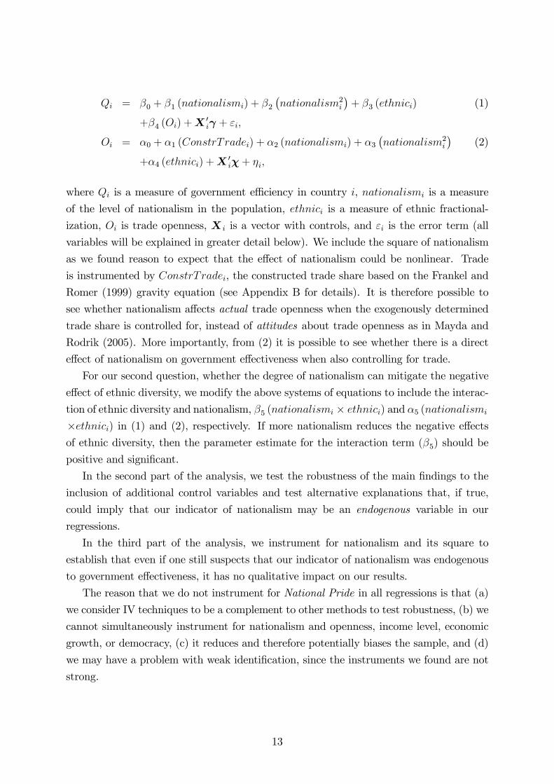
Qi = �0 + �1 (nationalismi) + �2�nationalism2

i

�+ �3 (ethnici) (1)

+�4 (Oi) +X0i + "i;

Oi = �0 + �1 (ConstrTradei) + �2 (nationalismi) + �3�nationalism2

i

�(2)

+�4 (ethnici) +X0i�+ �i;

where Qi is a measure of government e¢ ciency in country i, nationalismi is a measure

of the level of nationalism in the population, ethnici is a measure of ethnic fractional-

ization, Oi is trade openness, X i is a vector with controls, and "i is the error term (all

variables will be explained in greater detail below). We include the square of nationalism

as we found reason to expect that the e¤ect of nationalism could be nonlinear. Trade

is instrumented by ConstrTradei, the constructed trade share based on the Frankel and

Romer (1999) gravity equation (see Appendix B for details). It is therefore possible to

see whether nationalism a¤ects actual trade openness when the exogenously determined

trade share is controlled for, instead of attitudes about trade openness as in Mayda and

Rodrik (2005). More importantly, from (2) it is possible to see whether there is a direct

e¤ect of nationalism on government e¤ectiveness when also controlling for trade.

For our second question, whether the degree of nationalism can mitigate the negative

e¤ect of ethnic diversity, we modify the above systems of equations to include the interac-

tion of ethnic diversity and nationalism, �5 (nationalismi � ethnici) and �5 (nationalismi

�ethnici) in (1) and (2), respectively. If more nationalism reduces the negative e¤ects

of ethnic diversity, then the parameter estimate for the interaction term (�5) should be

positive and signi�cant.

In the second part of the analysis, we test the robustness of the main �ndings to the

inclusion of additional control variables and test alternative explanations that, if true,

could imply that our indicator of nationalism may be an endogenous variable in our

regressions.

In the third part of the analysis, we instrument for nationalism and its square to

establish that even if one still suspects that our indicator of nationalism was endogenous

to government e¤ectiveness, it has no qualitative impact on our results.

The reason that we do not instrument for National Pride in all regressions is that (a)

we consider IV techniques to be a complement to other methods to test robustness, (b) we

cannot simultaneously instrument for nationalism and openness, income level, economic

growth, or democracy, (c) it reduces and therefore potentially biases the sample, and (d)

we may have a problem with weak identi�cation, since the instruments we found are not

strong.

13

3.2 Data on government e¤ectiveness

We use Government E¤ectiveness as the dependent variable. This is one of the World

Bank�s Governance Indicators (Kaufmann et al., 2008), designed by combining a large

number of di¤erent measures from a wide range of sources to gauge the quality of gov-

ernance. More exactly, Government E¤ectiveness is constructed to indicate the gov-

ernment�s ability to �produce and implement good policies and deliver public goods�

(Kaufmann et al., 2003). The sources measure aspects such as how well the government

handles health services and education, how satis�ed people are with the infrastructure,

the level of trust in the government, bureaucratic delays, the strength and expertise of

the bureaucracy, how e¢ ciently the government uses resources, and so on. Hence, the

variable captures central aspects of the quality of government, as examined by La Porta

et al. (1999), and is in line with Miguel (2004) by capturing the quality of public service

delivery.

The main argument for combining a large number of measures is that while the actual

level of government e¤ectiveness cannot be directly observed, each individual measure

contributes a signal about the true level of governance. The indicator is therefore more

informative about the true level of government e¤ectiveness than any of the individual

measures. As often is the case with indicators of institutional quality, countries with high

levels of Government E¤ectiveness tend to score high also in terms of other governance

measures.

3.3 Data on nationalism

A useful indicator of nationalism needs to capture both that individuals feel tied to a

nation and the intensity of this tie. The latter aspect is central since it determines an

individual�s choice in a situation where she faces a choice between two actions, of which

one gives a higher private return than the other at the cost of a lower return to the nation.

Asking people whether they are nationalistic, and if so about the intensity of their

nationalism, is unlikely to provide a reliable measurement of these sentiments, since the

term nationalist is often considered to be pejorative. In the absence of a direct measure of

nationalism, the standard measure in the literature has been the level of national pride in

the population. This turns out be a good measure for our purposes since (1) an individual

who does not identify with a nation will obviously not report that she feels proud to be

a member of that nation, and (2) more pride should signal a closer emotional connection

to the nation and a stronger national identity.

Hence, the closer the ties to the nation and the stronger the pride of being a member

of it, the more important the welfare of the nation will be in the eyes of the individual,

and the more she accepts the authority of the government given that it is seen to rule

in the interest of the nation, the more altruistic she will act toward other nationals, and

14

the stronger the tendency for xenophobia and skepticism toward ideas, techniques, and

goods believed to violate national traditions will be. Also, an individual who does not

feel tied to (and hence is not proud to be a member of) a nation will either feel tied to

another nation or not pledge allegiance to any nation. Such an individual is not as likely

to accept the authority of the government, to be willing to make sacri�ces for the good

of the country, or to be skeptical of ideas, techniques, and goods simply because they are

not in line with national traditions.

The World Values Survey (WVS) has since 1981 conducted detailed public opinion

surveys of beliefs and values in a multitude of areas and for a broad cross section of

countries.5 We make use of the following question from the WVS: �How proud are you to

be [�Nationality�]?�There are four possible responses: �very proud,��quite proud,��not

very proud,�or �not at all proud.�We assign the value 1 for �not at all proud�and 2 for

�not very proud�etc., and then calculate the average for each country. The maximum

range is hence 1 to 4.6 If a country is included in the surveys more than once, we use the

�gure from the most recent survey. This gives us a range from 1995 (Australia) to 2003

(Kyrgyz Republic and Saudi Arabia), with the most observations from 1999, for a sample

of 79 countries. In the forthcoming analysis, we refer to this variable as National Pride.

Calculating the mean over all survey periods gives a similar result.

The instruments for nationalism, created as indicators of a number of important his-

torical or cultural circumstances, will be discussed in Section 4.3 in relation to the results

obtained when they are used.

4 Results

Table 1 presents the descriptive statistics for the countries in our main sample.7 National

Pride has a mean of 3.41 and a standard deviation of 0.33, and since 3 = quite proud and

4 = very proud, people on average seem to be more than quite proud of their country. The

lowest scores (from 2.7 to 2.8) are found in Germany, Taiwan, Japan, The Netherlands,

and Russia. We �nd the highest scores (3.8-3.9) in Egypt, Venezuela, Morocco, Iran, and

Puerto Rico. The U.S. is not far behind with a score of 3.7.

A natural question given our empirical framework is whether National Pride can be

considered to be exogenous to Government E¤ectiveness. In Section 2.1, we learned that

there was no simple answer to what determines nationalism. The correlations between

National Pride and other variables tell us a similar story (see Panel A in Table 2).

5See www.worldvaluessurvey.org for more information.6Surveys such as ISSP cover fewer countries but include more detailed question. These have been

used to classify respondents as patriots or nationalists (de Figueiredo and Elkins, 2003), or as blind orconstructive patriots (Schatz et al., 1999). Even if one accepted such an approach, it is not possible withthe WVS data we employ.

7The main sample consists of the countries for which we have data for speci�cation (3.5).

15

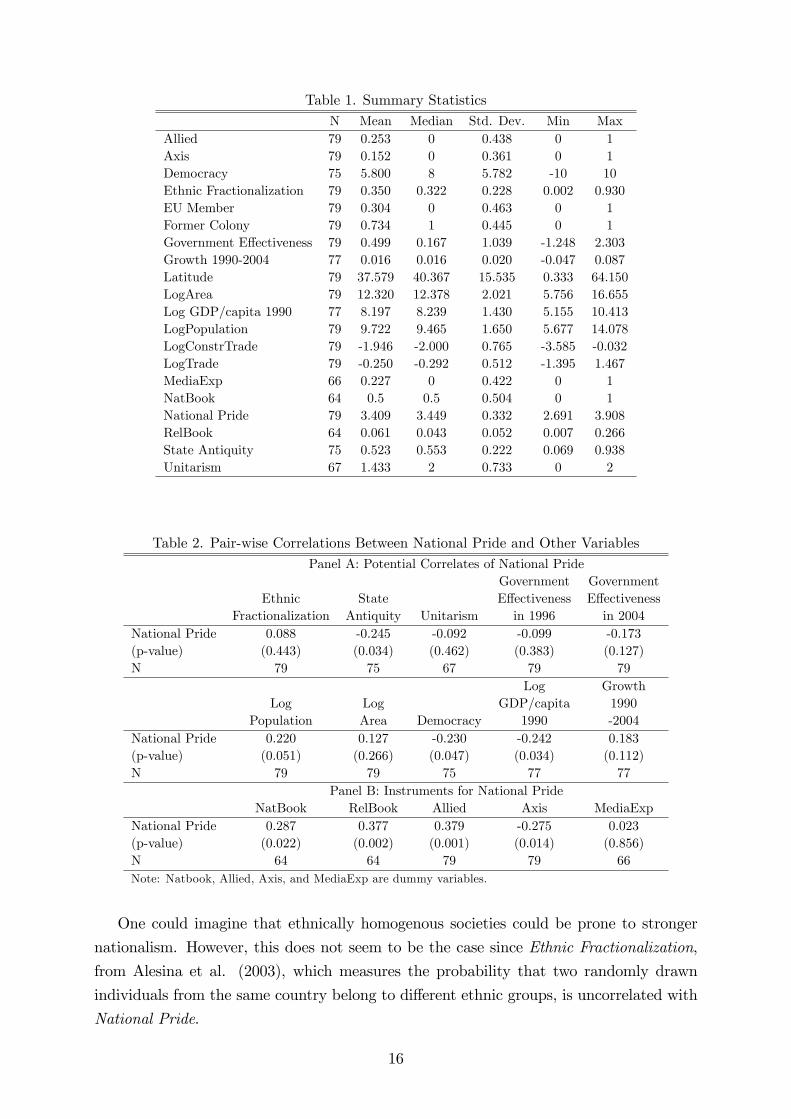
Table 1. Summary StatisticsN Mean Median Std. Dev. Min Max

Allied 79 0.253 0 0.438 0 1Axis 79 0.152 0 0.361 0 1Democracy 75 5.800 8 5.782 -10 10Ethnic Fractionalization 79 0.350 0.322 0.228 0.002 0.930EU Member 79 0.304 0 0.463 0 1Former Colony 79 0.734 1 0.445 0 1Government E¤ectiveness 79 0.499 0.167 1.039 -1.248 2.303Growth 1990-2004 77 0.016 0.016 0.020 -0.047 0.087Latitude 79 37.579 40.367 15.535 0.333 64.150LogArea 79 12.320 12.378 2.021 5.756 16.655Log GDP/capita 1990 77 8.197 8.239 1.430 5.155 10.413LogPopulation 79 9.722 9.465 1.650 5.677 14.078LogConstrTrade 79 -1.946 -2.000 0.765 -3.585 -0.032LogTrade 79 -0.250 -0.292 0.512 -1.395 1.467MediaExp 66 0.227 0 0.422 0 1NatBook 64 0.5 0.5 0.504 0 1National Pride 79 3.409 3.449 0.332 2.691 3.908RelBook 64 0.061 0.043 0.052 0.007 0.266State Antiquity 75 0.523 0.553 0.222 0.069 0.938Unitarism 67 1.433 2 0.733 0 2

Table 2. Pair-wise Correlations Between National Pride and Other VariablesPanel A: Potential Correlates of National Pride

Government GovernmentEthnic State E¤ectiveness E¤ectiveness

Fractionalization Antiquity Unitarism in 1996 in 2004National Pride 0.088 -0.245 -0.092 -0.099 -0.173(p-value) (0.443) (0.034) (0.462) (0.383) (0.127)N 79 75 67 79 79

Log GrowthLog Log GDP/capita 1990

Population Area Democracy 1990 -2004National Pride 0.220 0.127 -0.230 -0.242 0.183(p-value) (0.051) (0.266) (0.047) (0.034) (0.112)N 79 79 75 77 77

Panel B: Instruments for National PrideNatBook RelBook Allied Axis MediaExp

National Pride 0.287 0.377 0.379 -0.275 0.023(p-value) (0.022) (0.002) (0.001) (0.014) (0.856)N 64 64 79 79 66Note: Natbook, Allied, Axis, and MediaExp are dummy variables.

One could imagine that ethnically homogenous societies could be prone to stronger

nationalism. However, this does not seem to be the case since Ethnic Fractionalization,

from Alesina et al. (2003), which measures the probability that two randomly drawn

individuals from the same country belong to di¤erent ethnic groups, is uncorrelated with

National Pride.

16

Since the average distance to other people is smaller in smaller countries, people in

these countries could feel closer to each other and therefore feel a stronger sense of commu-

nity and national pride. Table 2 includes two measures of country size: LogPopulation and

LogArea. The correlations between National Pride and these two measures are positive,

indicating that the populations in small countries are less nationalistic, although only the

correlation with LogPopulation is statistically signi�cantly at the 10 percent level.

The negative correlation between National Pride and State Antiquity (from Bockstette

et al., 2002) shows that countries with less historical experience of an independent and

sovereign state apparatus, often indicating younger countries, are more likely to have more

proud populations.

Negative correlations are also found between National Pride and Democracy (mea-

sured as Polity2 from Polity IV project) and between National Pride and log(GDP/capita

1990). National Pride, which is measured for the years 1995-2003, is not correlated with

Government E¤ectiveness in 1996 (where 1996 is the earliest year for which data is avail-

able).

The pair-wise correlations between National Pride and the variables we will later use

as instruments for National Pride are also reported in Table 2. To avoid unnecessary

repetition, the design of the instruments, their correlations with National Pride, and the

estimates obtained when they are used will be discussed jointly in Section 4.3

In the regressions that will follow, we use values of National Pride for the years 1995-

2003 to explain Government E¤ectiveness in 2004. Moreover, in Section 4.2 we will

investigate alternative explanations that could imply that National Pride may be an

endogenous variable in our regressions. Lastly, in Section 4.3 we instrument for National

Pride to establish that even if one could still suspect that National Pride is endogenous

to Government E¤ectiveness, it does not drive our main results.

4.1 Nationalism and government e¤ectiveness

Although more National Pride is associated with less Government E¤ectiveness in the

�rst column in Table 3, the e¤ect is not signi�cant at standard levels of signi�cance (the p-

value is 0.12), and the linearity of this speci�cation does not correspond to the theoretical

discussion. Instead, the results presented in Column 2 show that there is a clear nonlinear

association between nationalism and government e¤ectiveness. This is, as we shall see, a

robust result. The nonlinear e¤ect indicates that at lower levels of National Pride there

is a positive e¤ect on Government E¤ectiveness while the e¤ect changes sign at higher

levels.

In the third column, we include Ethnic Fractionalization along with our baseline con-

trol variables �dummies for Legal Origin following La Porta et al. (1999), and a dummy

for NeoEurope �and this has only a marginal e¤ect on the parameter estimates for Na-

17

tional Pride and its square. The coe¢ cient for Ethnic Fractionalization has the expected

negative sign. The inclusion of the NeoEurope dummy, taking the value one for Australia,

Canada, New Zealand, and USA and zero for all other countries, is motivated not by these

countries having unusual values in terms of National Pride or Government E¤ectiveness

but by their unusual character as rich democratic settler colonies and their unusual com-

bination of both high National Pride and high Government E¤ectiveness. The inclusion

of a dummy for NeoEurope is not uncommon in cross-country regressions.

Table 3. Relationship Between Pride and Government E¤ectivenessDep. Var Government E¤ectiveness in 2004

(3.1) (3.2) (3.3) (3.4) (3.5)OLS OLS OLS OLS 2SLS

Panel A: OLS / Second Stage ResultsNational Pride -0.54 19.17*** 14.82*** 14.07*** 13.55***

(0.34) (6.35) (5.44) (4.82) (4.69)(National Pride)2 -2.97*** -2.42*** -2.27*** -2.16***

(0.94) (0.81) (0.71) (0.70)Ethnic Fractionalization -1.10*** -1.04*** -1.00***

(0.41) (0.36) (0.34)LogTrade 0.64*** 1.09***

(0.12) (0.18)Constant 2.35* -29.96*** -21.24** -20.26** -19.58**

(1.18) (10.59) (9.17) (8.18) (7.90)Legal Origin & NeoEurope No No Yes Yes YesN 79 79 79 79 79R2 0.030 0.113 0.614 0.693 0.654

Panel B: First Stage Results for LogTradeLogConstrTrade 0.43***

(0.07)National Pride -2.43a

(2.81)(National Pride)2 0.33a

(0.44)Ethnic Fractionalization -0.04

(0.21)Constant 5.09

(5.16)Legal Origin & NeoEurope YesF(LogConstrTrade) 43.04Note: Robust standard errors in parentheses. *** p<0.01, ** p<0.05, * p<0.1. anot

jointly signi�cant at the 10% level.

The legal origin is either British, French, Socialist, German, or Scandinavian. Coun-

tries with Socialist legal origin have signi�cantly worse, and countries with Scandinavian

legal origin have signi�cantly better, government e¤ectiveness than countries with British

legal origin, which is the excluded category.

The speci�cation in Column 4 includes LogTrade, resulting in only modest changes in

the coe¢ cients for National Pride and (National Pride)2. The positive coe¢ cient for trade

18

indicates that it may work as a disciplining device, in the sense that more open countries

are subject to higher competitive pressure and therefore implement more e¤ective policies.

LogTrade could here clearly be endogenous due to the plausible simultaneity between

openness and government e¤ectiveness. Therefore, the results in Column 5 are from

a two-stage procedure where LogTrade is instrumented for with LogConstrTrade as the

excluded instrument. LogConstrTrade is in turn estimated using a gravity equation similar

to in Frankel and Romer (1999), details of which are presented in Appendix B.

By instrumenting for LogTrade we can also investigate whether National Pride has

a direct e¤ect on LogTrade, but National Pride (and its square) is not signi�cant in the

�rst stage of speci�cation (3.5). While Mayda and Rodrik (2005) �nd that countries

with more nationalistic sentiments have less pro-trade attitudes, our results imply that

nationalistic sentiments may not a¤ect actual trade �ows. Turning to the second stage,

the coe¢ cient for LogTrade is larger than it was in the OLS estimation in (3.4). This

is similar to Frankel and Romer (1999), who �nd that OLS understates the relationship

between trade and income per capita.

A multitude of studies have shown that there is a strong geographical component of

trade, i.e., smaller countries and countries closer to each other trade more. This compo-

nent should not be a¤ected by nationalism or a preference for protectionism. Though the

coe¢ cient for trade is larger in speci�cation (3.5), the coe¢ cients for National Pride and

(National Pride)2 are quite stable despite the use of predicted rather than actual trade

share. This is another indication that the link from nationalism to government e¤ective-

ness does not go via less openness, since removing the endogenous part of trade from the

regression has only a moderate e¤ect on the estimates of the national pride variables.

To illustrate the nonlinear relationship between National Pride and Government Ef-

fectiveness in speci�cation (3.5), Figure 1 depicts the �component-plus-residual plot,�

which is used to illustrate functional form.8 The �gure makes it evident that the e¤ect of

more National Pride is �rst positive and then negative. The estimates in (3.5) actually

indicate that the e¤ect of more National Pride is positive up to a value of 3.13 (where 3

corresponds to �quite proud�), but that more nationalism is associated with worse scores

on Government E¤ectiveness at higher levels of National Pride.

Though the graph illustrates a distinct hump-shaped relationship, most countries lie

in the region where more nationalism is associated with worse government e¤ectiveness.

For the countries that lie in the region where more nationalism is associated with better

government e¤ectiveness, the potential gains seem to be moderate. Thus, we must con-

clude that while promotion of nationalism may be a marginally good idea in some cases,

8To adequately illustrate a partial relationship from a regression speci�cation with this number ofexplanatory variables is of course not possible. One can approximately graph the relationship using an�added variables plot�to assess the presence of outliers, or a �component-plus-residuals plot�to assessthe functional form.

19

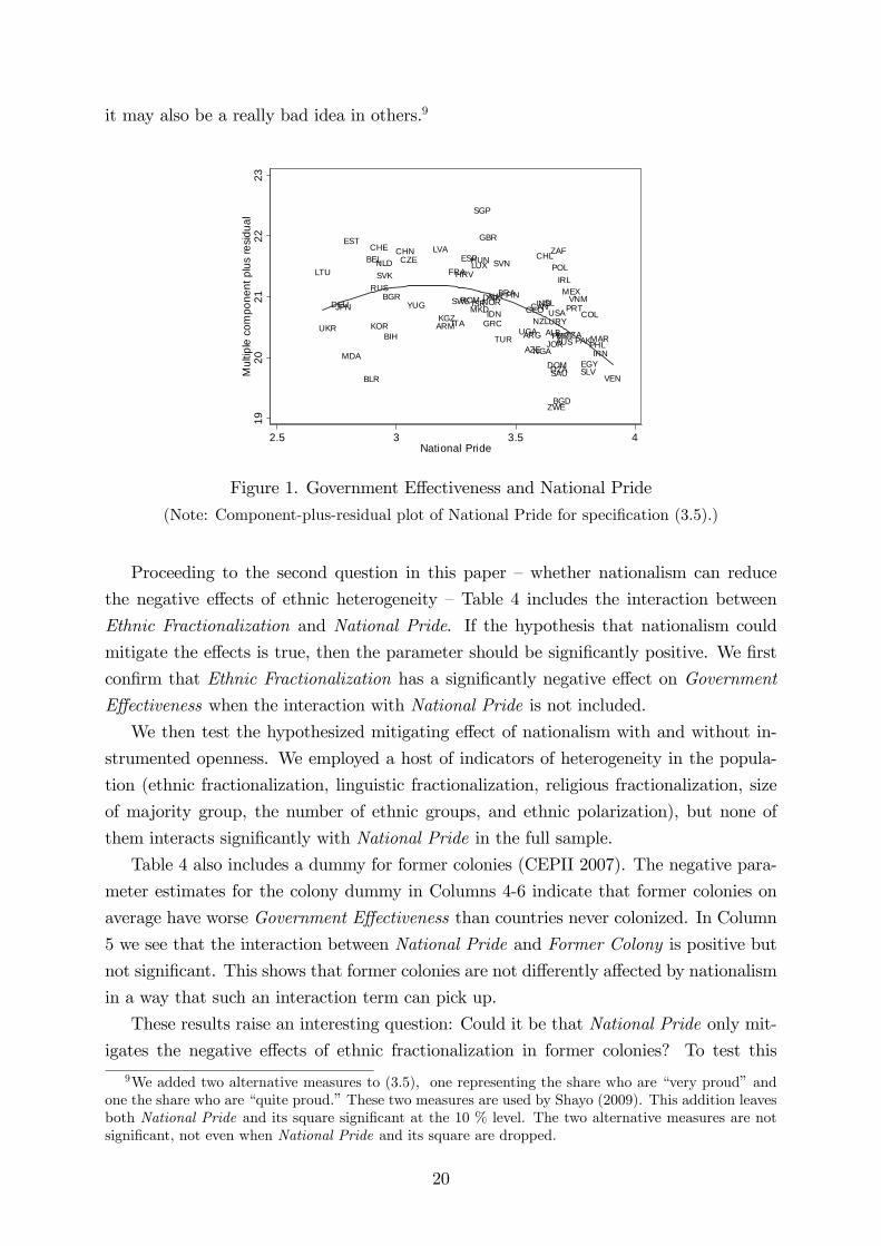
it may also be a really bad idea in others.9

LTU

UKR

DEUJPN

MDA

EST

BLR

BEL

CHE

RUS

KOR

NLD

SVK

BIH

BGR

CHNCZE

YUG

LVA

ARMKGZ

FRA

ITA

SWE

HRV

ESP

ROMISR

LUX

MKD

HUN

SGP

GBR

NORDNK

GRCIDN

AUT

SVN

TUR

BRAFIN

UGAARG

AZE

GEOCAN

NZL

NGA

IND

CHL

ISL

ALB

JOR

ZWE

USA

DOM

URY

ZAF

DZASAU

POL

PER

BGD

IRL

AUSMLT

MEX

TZA

PRTVNM

PAK

SLVEGY

COL

PHLMAR

IRN

VEN

19

20

21

22

23

Mu

ltip

le c

om

po

ne

nt

plu

s r

esid

ua

l

2.5 3 3.5 4National Pride

Figure 1. Government E¤ectiveness and National Pride

(Note: Component-plus-residual plot of National Pride for speci�cation (3.5).)

Proceeding to the second question in this paper �whether nationalism can reduce

the negative e¤ects of ethnic heterogeneity �Table 4 includes the interaction between

Ethnic Fractionalization and National Pride. If the hypothesis that nationalism could

mitigate the e¤ects is true, then the parameter should be signi�cantly positive. We �rst

con�rm that Ethnic Fractionalization has a signi�cantly negative e¤ect on Government

E¤ectiveness when the interaction with National Pride is not included.

We then test the hypothesized mitigating e¤ect of nationalism with and without in-

strumented openness. We employed a host of indicators of heterogeneity in the popula-

tion (ethnic fractionalization, linguistic fractionalization, religious fractionalization, size

of majority group, the number of ethnic groups, and ethnic polarization), but none of

them interacts signi�cantly with National Pride in the full sample.

Table 4 also includes a dummy for former colonies (CEPII 2007). The negative para-

meter estimates for the colony dummy in Columns 4-6 indicate that former colonies on

average have worse Government E¤ectiveness than countries never colonized. In Column

5 we see that the interaction between National Pride and Former Colony is positive but

not signi�cant. This shows that former colonies are not di¤erently a¤ected by nationalism

in a way that such an interaction term can pick up.

These results raise an interesting question: Could it be that National Pride only mit-

igates the negative e¤ects of ethnic fractionalization in former colonies? To test this

9We added two alternative measures to (3.5), one representing the share who are �very proud�andone the share who are �quite proud.�These two measures are used by Shayo (2009). This addition leavesboth National Pride and its square signi�cant at the 10 % level. The two alternative measures are notsigni�cant, not even when National Pride and its square are dropped.

20

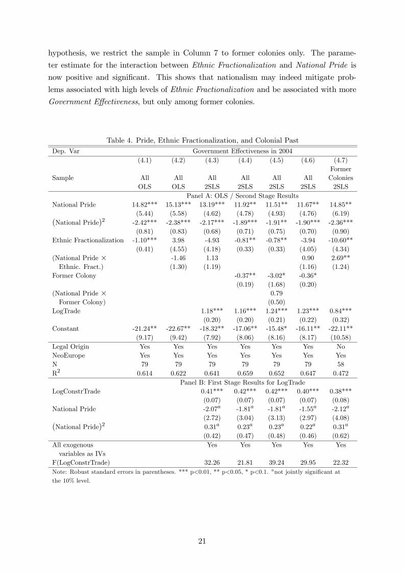
hypothesis, we restrict the sample in Column 7 to former colonies only. The parame-

ter estimate for the interaction between Ethnic Fractionalization and National Pride is

now positive and signi�cant. This shows that nationalism may indeed mitigate prob-

lems associated with high levels of Ethnic Fractionalization and be associated with more

Government E¤ectiveness, but only among former colonies.

Table 4. Pride, Ethnic Fractionalization, and Colonial PastDep. Var Government E¤ectiveness in 2004

(4.1) (4.2) (4.3) (4.4) (4.5) (4.6) (4.7)Former

Sample All All All All All All ColoniesOLS OLS 2SLS 2SLS 2SLS 2SLS 2SLS

Panel A: OLS / Second Stage ResultsNational Pride 14.82*** 15.13*** 13.19*** 11.92** 11.51** 11.67** 14.85**

(5.44) (5.58) (4.62) (4.78) (4.93) (4.76) (6.19)(National Pride)2 -2.42*** -2.38*** -2.17*** -1.89*** -1.91** -1.90*** -2.36***

(0.81) (0.83) (0.68) (0.71) (0.75) (0.70) (0.90)Ethnic Fractionalization -1.10*** 3.98 -4.93 -0.81** -0.78** -3.94 -10.60**

(0.41) (4.55) (4.18) (0.33) (0.33) (4.05) (4.34)(National Pride � -1.46 1.13 0.90 2.69**Ethnic. Fract.) (1.30) (1.19) (1.16) (1.24)

Former Colony -0.37** -3.02* -0.36*(0.19) (1.68) (0.20)

(National Pride � 0.79Former Colony) (0.50)

LogTrade 1.18*** 1.16*** 1.24*** 1.23*** 0.84***(0.20) (0.20) (0.21) (0.22) (0.32)

Constant -21.24** -22.67** -18.32** -17.06** -15.48* -16.11** -22.11**(9.17) (9.42) (7.92) (8.06) (8.16) (8.17) (10.58)

Legal Origin Yes Yes Yes Yes Yes Yes NoNeoEurope Yes Yes Yes Yes Yes Yes YesN 79 79 79 79 79 79 58R2 0.614 0.622 0.641 0.659 0.652 0.647 0.472

Panel B: First Stage Results for LogTradeLogConstrTrade 0.41*** 0.42*** 0.42*** 0.40*** 0.38***

(0.07) (0.07) (0.07) (0.07) (0.08)National Pride -2.07a -1.81a -1.81a -1.55a -2.12a

(2.72) (3.04) (3.13) (2.97) (4.08)(National Pride)2 0.31a 0.23a 0.23a 0.22a 0.31a

(0.42) (0.47) (0.48) (0.46) (0.62)All exogenous Yes Yes Yes Yes Yesvariables as IVs

F(LogConstrTrade) 32.26 21.81 39.24 29.95 22.32Note: Robust standard errors in parentheses. *** p<0.01, ** p<0.05, * p<0.1. anot jointly signi�cant at

the 10% level.

21

4.2 Robustness I: control variables and alternative explanations

In this subsection, we test the robustness of the e¤ect of nationalism to the addition

of various control variables. We continue to instrument for LogTrade throughout this

subsection.

The �rst two columns in Table 5 include the size measures LogPopulation and LogArea,

with the result that LogTrade is no longer signi�cant. The correlation between (predicted)

LogTrade and LogArea is -0.92, and they are jointly signi�cant. The constructed trade

share is not even signi�cant in the �rst stage, making it a weak instrument. Since popula-

tion size is a component of the constructed trade share, this e¤ect is to be expected.10 The

remainder of Table 5 includes controls for State Antiquity, Unitarism, European Union

membership (EU ), and absolute latitude (Latitude), and the e¤ect of National Pride is

still signi�cant and nonlinear. So far, National Pride and its square have not even been

jointly signi�cant in the �rst stage estimations, but in speci�cations (5.4) and (5.6) they

are. That they are jointly signi�cant in some speci�cations but not in others implies that

neither the existence nor the non-existence of an e¤ect of nationalism on openness can be

said to have strong support in the data.

A natural concern is that the results presented so far may not represent causal relation-

ships. Alternative explanations include reversed causality and that National Pride acts as

a proxy for some other more fundamental, but omitted, variable. Reversed causality (that

causality �ows from Government E¤ectiveness to National Pride) would for instance be

the case if people in countries with more e¤ective governments expressed a higher level

of National Pride as a result. We investigated this, in results not shown, by regressing

nationalism on government e¤ectiveness in 1996 (the earliest year available) and found

no e¤ect in that direction.11

It is possible that the signi�cant coe¢ cients for National Pride and (National Pride)2

are a result of the omission of �true�correlates of government e¤ectiveness, such as income,

economic growth, inequality, and level of democracy. The �rst of these potential concerns

draws on the earlier discussion on Shulman (2003), who argues that a strong national

identity can serve as an equalizer between rich and poor countries, and Shayo (2009),

who shows that poor people are more prone to identify with the nation. Similar to the

logic of nationalism in a country making the poor feel equal to the rich, a strong national

identity can make poor low-status countries feel equal to rich countries (Shulman, 2003).

10Appendix B shows that for a larger sample, LogConstrTrade is a valid instrument while also control-ling for LogArea and LogPopulation.11We allowed for nonlinearities and added control variables such as ethnic fractionalization, size of

population, openness, growth, and income, yet in none of the regressions was past government e¤ectivenessa signi�cant determinant of National Pride.

22

Table 5. Pride and More Control VariablesDep. Var Government E¤ectiveness in 2004

(5.1) (5.2) (5.3) (5.4) (5.5) (5.6)Panel A:Second Stage Results

National Pride 14.43** 16.96* 12.22*** 13.09*** 11.19*** 13.30***(6.07) (9.36) (4.68) (4.83) (3.18) (4.26)

(National Pride)2 -2.26** -2.63** -1.95*** -2.08*** -1.77*** -2.08***(0.89) (1.33) (0.70) (0.73) (0.47) (0.63)

Ethnic Fractionalization -0.95** -1.24* -1.01*** -1.60*** -0.50* -0.59**(0.42) (0.69) (0.37) (0.38) (0.30) (0.30)

LogPopulation 0.13(0.24)

LogArea 0.28(0.53)

State Antiquity 0.70(0.47)

Unitarism -0.21*(0.13)

EU member 0.79***(0.15)

Latitude 0.02***(0.01)

LogTrade 1.69 2.61 1.20*** 1.25*** 0.62*** 0.73***(1.20) (3.00) (0.26) (0.22) (0.20) (0.17)

Constant -22.63** -28.79 -17.84** -18.35** -16.74*** -20.68***(11.44) (20.57) (7.91) (7.97) (5.33) (7.24)

Legal Origin & NeoEurope Yes Yes Yes Yes Yes YesN 79 79 75 67 79 79R2 0.514 0.201 0.642 0.698 0.782 0.738

Panel B: First Stage Results for LogTradeLogConstrTrade 0.22 0.11 0.38*** 0.51*** 0.44*** 0.50***

(0.18) (0.17) (0.08) (0.07) (0.07) (0.09)National Pride -1.95a -2.29a -2.35a -3.10c -2.42a -2.68b

(3.00) (2.51) (2.98) (2.77) (2.88) (2.68)(National Pride)2 0.25a 0.31a 0.32a 0.42c 0.33a 0.34b

(0.47) (0.38) (0.46) (0.43) (0.45) (0.42)All exogenous yes yes yes yes yes yesvariables as IVs

F(LogConstrTrade) 1.55 0.46 23.56 52.88 35.28 32.96Note: Estimated with 2SLS. Robust standard errors in parentheses. *** p<0.01, ** p<0.05, * p<0.1.anot jointly signi�cant at the 10% level. bJointly signi�cant at the 10% level. cJointly signi�cant at

the 5% level.

Since richer countries can a¤ord bigger and better governments, income should ide-

ally always be held constant in the regressions. The econometric problem lies in the

fact that income is endogenous to government e¤ectiveness. We nonetheless include

Log(GDP/capita) in Column 1 of Table 6, and �nd that the nonlinear association be-

tween National Pride and Government E¤ectiveness is intact. With the reservation that

income is endogenous in this regression, we take the negative interaction term to indicate

that the negative side of nationalism is more pronounced in rich countries.

23

A second potential concern is that the level of National Pride may re�ect a satisfaction

with recent economic performance.12 With the caveat that Growth (1990-2004) is also

endogenous to government e¤ectiveness, we include it in speci�cation (6.2). Again, the

hump-shaped e¤ect of nationalism is intact.

A third potential concern is that the e¤ect of National Pride could re�ect that less

democratic nations are more likely to have a leadership that manipulates nationalism as a

means to improve its own power and position, without an intention to improve e¢ ciency.

It would not be straightforward to investigate this alternative explanation, but it is safe to

assume that manipulations are less likely to be e¤ective in real democracies. Speci�cation

(6.3) includes a measure of the quality of Democracy: Polity2 from the Polity IV project.

The results concerning National Pride remain even when we add both income, growth,

and democracy to the same speci�cation.

The sample used in Column 5 contains Democracies only. Democracies are countries

with a Polity2 score of six or more, since this is the threshold suggested by the coders of

Polity IV. That the e¤ect is clear and strong in the sample with only democratic countries

contradicts this alternative explanation.

As mentioned in Section 2.1, Shayo (2009) argues that poor people are more likely to

choose a national identity in countries with more acute income inequality, and that when

they do so their support for redistribution is lower. The argument could therefore be

made that National Pride somehow picks up the e¤ect of income inequality and that the

demand for redistribution could result in larger and potentially more ine¢ cient govern-

ments, �nanced by distortionary taxes. To test this, we include the Gini-coe¢ cient from

UNU-WIDER (Gini), the Demand for Redistribution from the World Values Surveys,

and Log(GDP/capita) and Tax Revenues/GDP from WDI (2007). The results presented

in (6.6) show with clarity that the hump-shaped e¤ect of National Pride is not driven

by inequality, the demand for redistribution, or the amount of taxes collected. We inter-

acted nationalism also with growth, democracy, and the Gini-coe¢ cient, but the e¤ect of

nationalism was not signi�cantly a¤ected by any of them.

We can thus reject the most likely alternative explanations. This lends implicit support

for the argument that nationalism really does a¤ect government e¤ectiveness.

The e¤ects of National Pride may be generalized to other indicators of institutions or

government e¤ectiveness. We used Transparency International�s Corruption Perceptions

Index (CPI ), as well as Control of Corruption and Rule of Law, both from Kaufmann et

al. (2008), as alternative dependent variables. The results were fully in line with those

where Government E¤ectiveness is used (not reported).

12Needless to say, this mechanism could in principle also result in a positive association between incomeand National Pride, but the negative correlation between these variables suggests otherwise.

24

Table 6. Income, Growth, and Democracy.Dep. Var Government E¤ectiveness in 2004

(6.1) (6.2) (6.3) (6.4) (6.5) (6.6)Sample All All All All Democ�s All

Panel A: Second Stage ResultsNational Pride 11.98*** 11.87*** 10.43** 8.89*** 15.33*** 7.92**

(4.03) (4.51) (4.37) (3.15) (5.17) (3.95)(National Pride)2 -1.41*** -1.92*** -1.66** -0.97** -2.42*** -1.24**

(0.53) (0.68) (0.66) (0.43) (0.78) (0.60)Ethnic Fractionalization -0.26 -0.74* -0.83** 0.11 -0.95** -0.18

(0.24) (0.38) (0.34) (0.24) (0.43) (0.28)Log (GDP/capita) 1.68*** 1.54*** 0.44***

(0.53) (0.39) (0.07)(National Pride � -0.36** -0.34***Log (GDP/capita)) (0.16) (0.11)

Growth (1990-2004) 7.64* 12.28***(4.29) (2.28)

Democracy 0.06*** 0.03***(0.01) (0.01)

Gini -0.02**(0.01)

Preference for -0.08Redistribution (0.07)

Tax Revenues / GDP -0.01(0.01)

LogTrade 0.40** 1.21*** 0.97*** 0.60*** 1.22*** 0.77***(0.20) (0.20) (0.26) (0.16) (0.26) (0.29)

Constant -27.12*** -16.99** -15.22** -21.76*** -22.18*** -13.69**(8.05) (7.49) (7.22) (6.01) (8.56) (6.22)

Legal Origin & NeoEurope Yes Yes Yes Yes Yes YesN 77 77 75 74 56 69R2 0.834 0.644 0.738 0.881 0.682 0.866

Panel B: First Stage Results for LogTradeLogConstrTrade 0.43*** 0.47*** 0.41*** 0.42*** 0.46*** 0.43***

(0.08) (0.05) (0.06) (0.08) (0.08) (0.10)National Pride -3.59a -3.49b -1.95c -4.77*a -5.04*b -0.35a

(2.69) (2.76) (3.04) (2.67) (2.80) (3.24)(National Pride)2 0.39a 0.48b 0.24c 0.54a 0.73*b 0.01a

(0.40) (0.43) (0.47) (0.40) (0.43) (0.50)All exogenous Yes Yes Yes Yes Yes Yesvariables as IVs

F(LogConstrTrade) 32.28 46.18 40.51 29.50 36.45 18.87Note: Estimated with 2SLS. Robust standard errors in parentheses. *** p<0.01, ** p<0.05, * p<0.1.

Democ�s are all countries with a Polity2 greater than or equal to six. anot jointly signi�cant at the

the 10% level. bJointly signi�cant at the 10% level. cJointly signi�cant at the 5% level.

When we include the potentially endogenous variables (Log(GDP/capita), Growth

(1990-2004), Democracy, etc.), we �nd that National Pride and (National Pride)2 are

jointly signi�cant in the �rst stages of some of the speci�cations in Tables 5 and 6. Taken

as a whole, Tables 3-6 therefore present quite indistinct results regarding the association

between nationalism and openness. Hence, even if some results suggest that nationalism

25

is associated with less actual openness, we must conclude that this link is far from robust.

To allow for unobserved country characteristics and to estimate the e¤ects of changes

in, as opposed to levels of, National Pride and Government E¤ectiveness, we need to

estimate the model on a panel data set. The WVS data stretches from 1981 to 2006,

but the number of times a country is included di¤ers (some countries are only included

once), and data on Government E¤ectiveness is only available from 1996 onward. This

means that the necessary overlap between National Pride and Government E¤ectiveness

is too small to allow panel data methods. An alternative dependent variable, the Quality

of Government, is used instead. The Quality of Government index is the average score

of three indexes: Corruption, Law and Order, and Bureaucratic Quality.13 We failed to

obtain signi�cant estimates when a within-groups estimator was used, quite possibly due

to the very modest variation over time in National Pride and Quality of Government.14

4.3 Robustness II: instrumenting for nationalism

To deal explicitly with the possible endogeneity of National Pride, we have identi�ed a

number of potential instruments for National Pride and the results obtained when these

are used are presented in Tables 7 and 8. Missing data limits the sample to 64 countries.

Pair-wise correlations between these �ve instruments and National Pride are reported in

Table 2, Panel B.

We hypothesize that populations that read more about their history and geography

are likely to develop a stronger emotional attachment to their country. To capture this,

NatBook is a binary variable that indicates whether the share of a country�s total book

production that is devoted to history and geography is higher than the median share

among the countries in the sample. RelBook is a continuous variable that indicates the

share of total book production that is devoted to religious material, and we hypothesize

that populations that read more material of this type will have a tendency to think that

group identities, and social returns, are important and/or to evaluate their country less

on a strictly rational basis.

NatBook and RelBook are both coded from 1995-1999 data (as these are the earliest

dates) obtained from UNESCO (2008). Their pair-wise correlations with National Pride

are indeed signi�cantly positive. They are also always signi�cantly positive when included

in the �rst stages in Table 7, hence the hypotheses �nd some support in the data.15 The

13The index Bureaucratic Quality is also included as one of the components in Government E¤ective-ness, and Government E¤ectiveness and Quality of Government are highly correlated (0.92). (Data from2002 due to data availability.)14An alternative approach similar to Krueger and Lindahl (2001) is to extract the maximum amount of

variation in the data by taking the latest observation minus the earliest. Yet, changes in National Pridedo not seem to signi�cantly explain changes in Quality of Government with this approach either.15The F�values in the �rst stages are higher, and the precision of the estimated e¤ects of nationalism is

better, if we include the share of a country�s total book production that is devoted to history or geographyrather than the dummy variable NatBook. Nevertheless, we use NatBook throughout as it is stronger in

26

�rst stage results from Table 7 are presented in Table 8, due to space considerations.

Table 7. Instrumenting for National PrideDep. Var. Government E¤ectiveness in 2004

(7.1) (7.2) (7.3) (7.4) (7.5)Panel A: LIML Estimates

National Pride 33.12** 34.02** 35.21** 42.79*** 37.97***(14.27) (13.40) (14.61) (16.25) (14.64)

(National Pride)2 -5.07** -5.21** -5.40** -6.60*** -5.82***(2.18) (2.03) (2.23) (2.47) (2.22)

Ethnic Fractionalization -1.88*** -1.87*** -1.85*** -1.75*** -1.73***(0.41) (0.41) (0.42) (0.48) (0.58)

NeoEurope Yes Yes Yes Yes YesN 64 64 64 64 56Instruments NatBook NatBook NatBook NatBook NatBook

Allied Allied RelBook Axis AlliedRelBook RelBook MediaExpPanel B: Endogenous Variables

National PrideF(excluded IVs) 10.07*** 8.09*** 10.59*** 10.03*** 11.60***

(National Pride)2

F(excluded IVs) 9.85*** 8.10*** 10.73*** 10.31*** 11.42***Panel C: Tests

Overid. test (p) n.a. 0.847 n.a. 0.409 0.768Endogeneity test (p) 0.170 0.121 0.118 0.046 0.175AR Wald Chi2(p) 0.033 0.022 0.025 0.003 0.008Note: Dependent variable is Government E¤ectiveness in 2004. Estimated with LIML.

Robust standard errors in parentheses, *** p<0.01, ** p<0.05, * p<0.1. Constants are

omitted from the table. The overid test is Hansen�s J. The endogeneity test is from

Baum et al. (2003). AR (Anderson Rubin) Wald Chi2 is a test of all instrumented

variables that is robust to weak instruments.

We also hypothesize that populations that were on the winning side in the WW2

are likely to feel more proud and have a stronger attachment to their country, while

populations that were on the losing side or remained neutral are less likely to value their

own countries� history highly. Allied indicates that the country was an Allied Power,

or a supporter of the Allied Powers during WW2. Axis indicates that the country was

a member or a supporter of the Axis (signatories and cosignatories of the Tripartite

Treaty), or was neutral during WW2. Of the 64 countries in the sample, 18 are counted

as Allied and 11 as Axis; see Appendix A for details.16 In line with the hypothesis,

Allied is signi�cantly positive and Axis is signi�cantly negative in the �rst stages of the

estimations. The instruments used in Table 7 are not strong, wherefore LIML (Limited

Information Maximum Likelihood) is used as this is more reliable when instruments are

weak (Stock and Yogo, 2002).

regressions where we also include RelBook.16Note also that when Allied (alt. Axis) is used as an instrument, the omitted category consists of

both Axis (alt. Allied) and the 35 countries that are neither Allied nor Axis.

27

Allied and NatBook are used as instruments for National Pride and its square in

the �rst column in Table 7, and Ethnic Fractionalization and NeoEurope are included

as control variables.17 Satisfyingly, the inverted U-shaped relationship between National

Pride and Government E¤ectiveness is found also when we instrument for National Pride.

The estimates for instrumented National Pride and (National Pride)2 are both of higher

magnitude than their OLS counterparts, which could indicate that the OLS estimates

su¤er from measurement-driven attenuation bias. The coe¢ cients in (7.1) imply that the

strongest e¤ect on Government E¤ectiveness is found when National Pride is 3.27, which

is quite close to the corresponding value of 3.13 found in speci�cation (3.5).

In (7.2), we can test whether the model is overidenti�ed since RelBook is added as

instrument. The test result clearly indicates that the instruments are valid. As always,

these tests require that at least one of the instruments is valid, but we have also con�rmed

that none of the instruments has an e¤ect on Government E¤ectiveness besides their

indirect e¤ect on nationalism.18

The �rst stage F-values are highly signi�cant, but since we have robust standard errors

we cannot formally test whether the instruments are weak with the test devised in Stock

and Yogo (2002). Instead we perform the Anderson-Rubin Wald Chi2 test, which is a test

of whether the instrumented variables have a signi�cant e¤ect on the dependent variable.

The test, designed to be robust to weak instruments, shows that there is a signi�cant

e¤ect of National Pride and its square in all columns in Table 7.

In Column 3, we drop Allied from the list of instruments, and in Column 4, we

include Axis as an additional instrument, and in both cases the estimates are highly

signi�cant. All columns report the results from Baum et al.�s (2003) test for endogeneity

of the instrumented variable, but it is only in speci�cation (7.4) that this test suggest that

National Pride and (National Pride)2 actually are endogenous and should be instrumented

for rather than included as exogenous measures.

In the �nal column of Table 7, we replace RelBook with another alternative instru-

ment, MediaExp. We hypothesize that a population whose popular culture is more widely

spread over the world is more proud of their country. MediaExp is a dummy for exporting

more than importing of visual arts and audiovisual media in 2003 (which is the earliest

year with data on the country level). The data for MediaExp is obtained from tables

in UNESCO (2005), and in line with the hypothesis that MediaExp has a signi�cantly

17The dummies for German, Socialist, French, and Scandinavian countries would naturally pick upmuch of the same variation as Allied or Axis, but we hold that the latter two are more likely to trulya¤ect nationalism.18We added the instruments separately as explanatory variables in speci�cations where they are not

used as excluded instruments, and found that none of them has a statistically signi�cant direct e¤ecton Government E¤ectiveness. We found this when BookRel and MediaExp were added separately asexplanatory variables in (7.1), and when Allied and Axis were added separately in (7.3). Natbook is thestrongest of our instruments, and the �rst stage F-values are insu¢ cient if it is not included. Instead, weincluded Natbook in speci�cation (3.5) and found that it has no signi�cant direct e¤ect on GovernmentE¤ectiveness.

28

positive e¤ect when included in the �rst stage estimations in Table 7, and the coe¢ cients

for the instrumented National Pride and (National Pride)2 are both signi�cant.19 Ad-

mittedly, the late date (2003) could be problematic, but the overidenti�cation test clearly

indicates that the instruments in (7.5) are valid.

Table 8. Instrumenting for National Pride. First Stage Result for Table 7(7.1) (7.2) (7.3) (7.4) (7.5)

Panel A: First Stage Estimates for National PrideNatBook 0.23** 0.22** 0.22** 0.19* 0.25***

(0.09) (0.09) (0.09) (0.10) (0.09)Allied 0.30*** 0.25*** 0.37***

(0.08) (0.08) (0.08)RelBook 2.07*** 2.43*** 2.24***

(0.65) (0.56) (0.56)Axis -0.19*

(0.10)MediaExp 0.17*

(0.10)Ethnic Fractionalization 0.30 0.21 0.23 0.13 0.19

(0.19) (0.18) (0.19) (0.19) (0.22)NeoEurope Yes Yes Yes Yes YesF(excluded IVs) 10.07*** 8.09*** 10.59*** 10.03*** 11.60***Partial R2 0.253 0.352 0.247 0.289 0.352Shea�s Partial R2 0.152 0.172 0.135 0.154 0.178

Panel B: First Stage Estimates for (National Pride)2

NatBook 1.44** 1.35** 1.37** 1.15* 1.55**(0.61) (0.58) (0.63) (0.64) (0.58)

Allied 1.99*** 1.72*** 2.48***(0.54) (0.55) (0.56)

RelBook 13.94*** 16.31*** 15.07***(4.39) (3.72) (3.74)

Axis -1.28**(0.64)

MediaExp 1.16*(0.67)

Ethnic Fractionalization 1.93 1.33 1.48 0.83 1.25(1.27) (1.18) (1.27) (1.28) (1.49)

NeoEurope Yes Yes Yes Yes YesF(excluded IVs) 9.85*** 8.10*** 10.73*** 10.31*** 11.42***Partial R2 0.247 0.350 0.240 0.284 0.347Shea�s Partial R2 0.149 0.171 0.131 0.152 0.175N 64 64 64 64 56Note: First stage results from the LIML estimations of the speci�cation in Table 7.Robust standard errors in parentheses, *** p<0.01, ** p<0.05, * p<0.1. Constantsare omitted from the table. Shea�s Partial R2 takes intercorrelations amonginstruments into account.

In sum, the results in this section show that there is an inverted U-shaped relation-

ship between National Pride and Government E¤ectiveness also when we instrument for

National Pride.19Even if the pair-wise correlation between MediaExp and National Pride is low and not signi�cant

(see Table 2), the results in speci�cation (7.5) show that the partial correlation is signi�cant when theother factors are held constant.

29


The theoretical literature debates the importance of nation-building and nationalism for

the economic and political performance of societies. However, empirical evidence that the

creation of a national unity is a worthwhile policy alternative has been largely absent.

We �nd that the level of nationalism, measured by the level of national pride among the

population, has an inverted U-shaped relationship with government e¤ectiveness. Though

data limitations restrict an adequate examination over time, the cross-country evidence

is clear: More nationalism is associated with better government e¤ectiveness at low levels

of nationalism, while the e¤ect is the opposite at high levels of nationalism. This �nding

is robust to a wide range of speci�cations and when nationalism is instrumented for with

instruments that represent a number of historical and cultural circumstances.

We �nd some support for the idea that nation-building, in the sense of a higher level

of national pride, can resolve potential problems that come with high levels of ethnic frac-

tionalization, but only in former colonies. Finally, the issue of whether more nationalism

entails lower trade �ows has not been settled. Previous research on survey data has shown

that national pride is negatively associated with pro-trade attitudes on the micro level,

but this does not seem to translate into a robustly negative relationship between attitudes

and actual trade �ows on the macro level. The association is marginally signi�cant in

some of our speci�cations and not signi�cant in others.

A policy designed to create, strengthen, or sustain a sense of national unity must be

one of the most dramatic policies conceivable: It has the potential to a¤ect not only how

people view themselves and others, but their actual identities, political views, and, in the

end, actions. The fact that there have been so few attempts to systematically investigate

the potential e¤ects of such policies has by no means deterred policy makers from pursuing

them. This neglect by empirical social scientists has, however, contributed to a situation

where important decisions have been made by policy makers who have lacked systematic

knowledge of whether the likely outcome is good or bad.

Taken seriously, the results in this paper suggest that most countries already have too

nationalistic populations, and probably would function better if these sentiments where

downplayed. Yet some countries, especially former colonies with fragmented populations,

should still consider policies of nation-building. However, the latter advice comes with

an important caveat: Nationalism can have serious negative e¤ects, both for individuals

and for societies. Prejudice and discrimination also entail non-economic costs, and the

negative consequences of nationalism will probably become increasingly problematic in

the future, as the free �ow of people and ideas is unlikely to become less important.

As such, we believe that in all but perhaps a few countries, an active encouragement of

nationalistic sentiments is likely to have negative e¤ects on aggregate performance and

individual welfare.

30

ReferencesAhlerup, P. and O. Olsson (2007) �The Roots of Ethnic Diversity�Working Papers in

Economics No. 281, University of Gothenburg.

Akerlof, G.A. and R.E. Kranton (2000) �Economics and Identity� Quarterly Journal ofEconomics, 115(3):715-53.

Alesina, A., R. Baqir, and W. Easterly (1999) �Public Goods and Ethnic Divisions�Quar-terly Journal of Economics, 114(4):1243-84.



Anderson, B. (1983) Imagined Communities: Re�ections on the origin and spread of nation-alism, Repr. 1992, London: Verso.

Barrington, L.W. (2006) �Nationalism & Independence�in After Independence: Making andProtecting the Nation in Postcolonial and Postcommunist States (ed. L.W. Barrington),Ann Arbor: University of Michigan Press.

Baum, C.F., M.E. Scha¤er, and S. Stillman (2003) �Instrumental variables and GMM:Estimation and testing�Stata Journal, 3:1-31.

Bernhard, H., U. Fischbacher, and E. Fehr (2006) �Parochial Altruism in Humans�Nature,442:912�15.

Bockstette, V., A. Chanda, and L. Putterman. (2002) �States and Markets: The Advantageof an Early Start�Journal of Economic Growth, 7:347-69.

Bowles, S. (2008) �Con�ict: Altruism�s midwife�Nature, 456:326-27.

CEPII (2007) �Centre d�Etude Prospective et d�Informations Internationales,�available on-line at http://www.cepii.fr/.

Correlates of War project (2008), available online at http://www.correlatesofwar.org/.

de Figueiredo, R.J.P. Jr. and Z. Elkins (2003) �Are Patriots Bigots? An Inquiry into theVices of In-Group Pride�American Journal of Political Science, 47(1):171�88.

Easterly, W. and R. Levine (1997) �Africa�s growth tragedy: policies and ethnic divisions�Quarterly Journal of Economics, 112(4):1203-50.

E¤erson, C., R. Lalive, and E. Fehr (2008) �The Coevolution of Cultural Groups and IngroupFavoritism�Science, 321:1844-9.

Evans, M.D.R and J. Kelley (2002) �National Pride in the Developed World�InternationalJournal of Public Opinion Research, 14(3):303-8.

Hylland Eriksen, T. (1993) Ethnicity and Nationalism: Anthropological Perspectives, Repr.2002, London: Pluto Press.

Fearon, J.D. (2003) �Ethnic and Cultural Diversity by Country� Journal of EconomicGrowth, 8:195-222.

Fowler, J. and C. Kam (2007) �Beyond the Self: Social Identity, Altruism, and PoliticalParticipation.�Journal of Politics, 69(3):813�27.

Frankel, J.A. and D. Romer (1999) �Does Trade Cause Growth?�American Economic Re-view, 89(3):379-99.

Frankel, J.A. and A.K. Rose (2002) �An estimate of the e¤ect of common currencies ontrade and income�Quarterly Journal of Economics, 117(2):437-66.


31

Glaeser, E.L., D.I. Laibson, J.A. Scheinkman, and C.L. Soutter (2000) �Measuring Trust�Quarterly Journal of Economics, 115(3):811-46.

Goette, L., D. Hu¤man, and S. Meier (2006) �The Impact of Group Membership on Co-operation and Norm Enforcement: Evidence Using Random Assignment to Real SocialGroups�American Economic Review, 96(2):212-6.

Herbst, J. (2000) States and Power in Africa, Princeton: Princeton University Press.

Kaelberer, M. (2004) �The euro and European identity: symbols, power and the politics ofEuropean monetary union�Review of International Studies, 30:161�78.

Kaufmann, D., A. Kraay, and M. Mastruzzi. (2003) �Governance Matters III: GovernanceIndicators for 1996-2002�World Bank Policy Research Working Paper 3106.

Kaufmann, D., A. Kraay, and M. Mastruzzi. (2008) �Governance Matters VII: Aggregateand Individual Governance Indicators 1996-2007�World Bank Policy Research WorkingPaper 4654.

Krueger, A. B. and M. Lindahl. (2001) �Education for Growth: Why and For Whom?�Journal of Economic Literature, 39:1101-36.

La Porta, R., F. Lopez-de-Silanes, A. Shleifer, and R. Vishny (1999) �The Quality of Gov-ernment�Journal of Law, Economics, & Organizations, 15(1):222-79.

Mayda, A.N. and D. Rodrik (2005) �Why are some people (and countries) more protectionistthan others?�European Economic Review, 49:1393-430.

McFarland, S. and M. Mathews (2005) �Who Cares About Human Rights?�Political Psy-chology, 26(3):365�85.

Miguel, E. (2004) �Tribe or Nation? Nation-building and Public Goods in Kenya versusTanzania�World Politics, 56:327-62.

Miguel, E. and M.K. Gugerty (2005) �Ethnic diversity, social sanctions, and public goodsin Kenya�Journal of Public Economics, 89:2325-68.

Nakano, T. (2004) �Theorising economic nationalism�Nations and Nationalism, 10(3):211�29.

Olsson, O. and G. Hansson. (2006) �Country Size and the Rule of Law: ResuscitatingMontesquieu�Working Papers in Economics No. 200, University of Gothenburg.

Pellegrini, L. and R. Gerlagh (2008) �Causes of corruption: a survey of cross-country analysesand extended results�Economics of Governance, 9(3):245-63.

Persson, T. and G. Tabellini. (2003) The Economic E¤ects of Constitutions, Cambridge:The MIT Press.

Polity IV Project (2008), available online at http://www.systemicpeace.org/polity/polity4.htm.

Pye, L. W. (1971) �Identity and the Political Culture�in Crises and Sequences in PoliticalDevelopment (ed. Binder, L. et al.), Princeton: Princeton University Press.

Schatz, R.T., E. Staub, and H. Lavine (1999) �On the Varieties of National Attachment:Blind Versus Constructive Patriotism�Political Psychology, 20(1):151-74.

Schatz, R.T. and H. Levine (2007) �Waving the Flag: National Symbols, Social Identity,and Political Engagement�Political Psychology, 28(3):329-55.

Shayo, M. (2009) �A Model of Social Identity with and Application to Political Economy:Nation, Class, and Redistribution�American Political Science Review, 103(2):147-74.

Shulman, S. (2000) �Nationalist Sources of International Economic Integration� Interna-tional Studies Quarterly, 44:365-90.

32

Shulman, S. (2002) �Challenging the Civic/Ethnic and West/East Dichotomies in the Studyof Nationalism�Comparative Political Studies, 35:554-85.

Shulman, S. (2003) �Exploring the Economic Basis of Nationhood�Nationalism and EthnicPolicies, 9(2):23-49.

Smith, A.D. (1986) The Ethnic Origin of Nations, Oxford: Basil Blackwell.

Smith, T.W. and S. Kim (2006) �National Pride in a Comparative Perspective: 1995/96 and2003/04�International Journal of Public Opinion Research, 18(1):127-36.

Stanford Encyclopedia of Philosophy (2008), available online at http://plato.stanford.edu/entries/nationalism.

Stephenson, C. (2005) �Nation-building� Beyond Intractability (eds. Guy Burgess andHeidi Burgess.) Con�ict Research Consortium, University of Colorado, Boulder. Posted:January 2005, available at http://www.beyondintractability.org/essay/nation_building/.

Stock, J.H. and M. Yogo (2002) �Testing for weak instruments in linear IV regression�NBERTechnical Working Paper No. 284.

Teorell, J., S. Holmberg, and B. Rothstein (2007) �The Quality of Government Dataset,version 1 July 07,�available online at http://www.qog.pol.gu.se.


Treisman, D. (2000) �The causes of corruption: a cross national study� Journal of PublicEconomics, 76:399-457.

UNESCO (2005) International Flows of Selected Cultural Goods and Services, 1994-2003,Montreal: UNESCO Institute for Statistics.

UNESCO (2008), available online at http://stats.uis.unesco.org/.

Verba, S. (1971) �Sequences and Development�in Crises and Sequences in Political Devel-opment (ed. L. Binder et al.), Princeton: Princeton University Press.

WDI (2007) World Development Indicators, available online at http://www.worldbank.org.

33

Appendix A. Sample and variable description

Table A1. The 79 countries included in main sampleCountry Code Region Income groupAustralia AUS East Asia and Paci�c High incomeJapan JPN East Asia and Paci�c High incomeKorea, Rep. KOR East Asia and Paci�c High incomeNew Zealand NZL East Asia and Paci�c High incomeSingapore SGP East Asia and Paci�c High incomeAustria AUT Europe and Central Asia High incomeBelgium BEL Europe and Central Asia High incomeCzech Republic CZE Europe and Central Asia High incomeDenmark DNK Europe and Central Asia High incomeEstonia EST Europe and Central Asia High incomeFinland FIN Europe and Central Asia High incomeFrance FRA Europe and Central Asia High incomeGermany DEU Europe and Central Asia High incomeGreece GRC Europe and Central Asia High incomeIceland ISL Europe and Central Asia High incomeIreland IRL Europe and Central Asia High incomeItaly ITA Europe and Central Asia High incomeLuxembourg LUX Europe and Central Asia High incomeMalta MLT Europe and Central Asia High incomeNetherlands NLD Europe and Central Asia High incomeNorway NOR Europe and Central Asia High incomePortugal PRT Europe and Central Asia High incomeSlovenia SVN Europe and Central Asia High incomeSpain ESP Europe and Central Asia High incomeSweden SWE Europe and Central Asia High incomeSwitzerland CHE Europe and Central Asia High incomeUnited Kingdom GBR Europe and Central Asia High incomeIsrael ISR M. East and N. Africa High incomeSaudi Arabia SAU M. East and N. Africa High incomeCanada CAN North America High incomeUnited States USA North America High incomeBulgaria BGR Europe and Central Asia Upper middleCroatia HRV Europe and Central Asia Upper middleHungary HUN Europe and Central Asia Upper middleLatvia LVA Europe and Central Asia Upper middleLithuania LTU Europe and Central Asia Upper middlePoland POL Europe and Central Asia Upper middleRomania ROM Europe and Central Asia Upper middleRussian Federation RUS Europe and Central Asia Upper middleSerbia/Montenegro YUG Europe and Central Asia Upper middleSlovak Republic SVK Europe and Central Asia Upper middleTurkey TUR Europe and Central Asia Upper middleArgentina ARG L.America and Caribbean Upper middleBrazil BRA L.America and Caribbean Upper middleChile CHL L.America and Caribbean Upper middleMexico MEX L.America and Caribbean Upper middleUruguay URY L.America and Caribbean Upper middleVenezuela, RB VEN L.America and Caribbean Upper middleSouth Africa ZAF Sub-Saharan Africa Upper middleChina CHN East Asia and Paci�c Lower middleIndonesia IDN East Asia and Paci�c Lower middlePhilippines PHL East Asia and Paci�c Lower middleAlbania ALB Europe and Central Asia Lower middleArmenia ARM Europe and Central Asia Lower middleAzerbaijan AZE Europe and Central Asia Lower middleBelarus BLR Europe and Central Asia Lower middleBosnia/Herzegovina BIH Europe and Central Asia Lower middleGeorgia GEO Europe and Central Asia Lower middleMacedonia, FYR MKD Europe and Central Asia Lower middle

34

Moldova MDA Europe and Central Asia Lower middleUkraine UKR Europe and Central Asia Lower middleColombia COL L.America and Caribbean Lower middleDominican Rep. DOM L.America and Caribbean Lower middleEl Salvador SLV L.America and Caribbean Lower middlePeru PER L.America and Caribbean Lower middleAlgeria DZA M.East and N.Africa Lower middleEgypt, Arab Rep. EGY M.East and N.Africa Lower middleIran, Islamic Rep. IRN M.East and N.Africa Lower middleJordan JOR M.East and N.Africa Lower middleMorocco MAR M.East and N.Africa Lower middleVietnam VNM East Asia and Paci�c Low incomeKyrgyz Rep. KGZ Europe and Central Asia Low incomeBangladesh BGD South Asia Low incomeIndia IND South Asia Low incomePakistan PAK South Asia Low incomeNigeria NGA Sub-Saharan Africa Low incomeTanzania TZA Sub-Saharan Africa Low incomeUganda UGA Sub-Saharan Africa Low incomeZimbabwe ZWE Sub-Saharan Africa Low income

The countries are classi�ed according to the World Bank into income and geographic location

groups. The economies are divided among income groups according to 2006 gross national

income (GNI) per capita. The World Bank sometimes refers to low-income and middle-income

economies as developing economies. By this de�nition, 30 out of the 79 countries in the sample

are developing countries.

Variable descriptions

Allied : Dummy for being an Allied Power or a supporter of the Allied e¤orts during WW2.

The following 18 countries in the sample used in Table 7 are coded as Allied: Argentina, Brazil,

Canada, Chile, Colombia, Egypt, El Salvador, Mexico, New Zealand, Peru, Russian Feder-

ation (Soviet Union), Saudi Arabia, South Africa, Turkey, United Kingdom, United States,

Uruguay, and Venezuela. Countries that were invaded, annexed, occupied, a colony, or did

not exist as free countries at the time of WW2 are coded as neither Allied nor Axis. Source:

Encyclopedia Britannica (www.britannica.com) supplemented with information from Wikipedia

(www.wikipedia.org) for some countries.

Axis: Dummy for being a member or a supporter of the Axis or neutral during WW2. Eleven of

the 64 countries in the sample used in Table 7 are coded as Axis (Bulgaria, Germany, Hungary,

Italy, Japan, Portugal, Romania, Slovakia, Spain, Sweden, and Switzerland). See also under

Allied above.

Control of Corruption: Source: Kaufmann et al. (2008).

Corruption Perceptions Index (CPI): Transparency International�s Corruption Perceptions In-

35

dex. Corruption is de�ned as the abuse of public o¢ ce for private gain. Source: Teorell et al.

(2007).

Democracy : Polity2 from the Polity IV project. Polity2 ranges from +10 (strongly democratic)

to -10 (strongly autocratic). The Democracy score used represents 31 December 2003. Source:

Polity IV Project (2008).

Democ�s: (Democracies) Countries that have a Polity2 score of six or higher. See also Democracy.

EU : Dummy for EU member countries.

Ethnic Fractionalization: Based on the Her�ndahl index; the probability that two randomly

drawn individuals from the same country belong to di¤erent groups. Source: Alesina et al.

(2003).

Former Colony : Dummy for having been subject to colonization for a �relatively long period of

time� and where the colonizing country had a �substantial participation in the governance of

the colonized country.�Source: CEPII (2007).

Gini : The Gini index of income inequality as reported by UNU-WIDER. The latest available

�gure, but not later than 2004, is used. Source: Teorell et al. (2007).

Government E¤ectiveness: Measuring the competence of the bureaucracy and the quality of

public service delivery. Source: Kaufmann et al. (2008).

Growth 1990-2004 : Annual growth rate in real GDP per capita from 1990 until 2004. GDP per

capita data from WDI (2007).

Latitude: Absolute latitude in degrees. Source: CEPII (2007).

Legal Origin: Identi�es the legal origin of the Company Law or Commercial Code for each

country. There are �ve possible origins: English Common Law, French Commercial Code,

Socialist/Communist laws, Scandinavian Commercial Code, and German Commercial Code.

Included as four dummy variables with English legal origin left as the excluded category. Source:

La Porta et al. (1999).

LogArea: Log of land area in km2. Source: WDI (2007).

Log GDP/capita in 1990 : in constant US$2000. Source: WDI (2007).

LogPopulation: Log of total population (2004). Source: WDI (2007).

LogTrade: Log of (exports + imports)/GDP divided by 100, all from 2004 in current local

currency units. Source: WDI (2007).

MediaExp: Dummy for exporting more than importing of visual arts and audiovisual media in

2003. Source: UNESCO (2005).

36

NatBook : Dummy for having a share of total book production devoted to history or geography

that is higher than the median in the sample. Average for 1995-1999. Source: UNESCO (2008).

NeoEurope: Dummy for Australia, Canada, New Zealand, USA.

National Pride: Question G006 from World Values Survey: �How proud are you to be [Nation-

ality]?� 1 = Not at all proud, 2 = not very proud, 3 = quite proud, 4 = very proud. (Note

that we have reversed the scoring in relation to WVS in order to have a high score re�ecting

a high degree of pride.) The latest possible data is used. For our sample of 79 countries, this

implies observations from 1995 to 2003. The mean value of national pride for each country is

then calculated, with respect to the weights (S017). The weights are used to better represent

the country as a whole.

Preference for Redistribution: Question E035 from World Values Survey. On the issue of income

inequality, the respondents are asked where on a scale from 1 to 10, where 1 represents �Incomes

should be made more equal�and 10 represents �We need larger income di¤erences as incentives,�

they would place themselves. The variable is the average �gure for each country from 1981 to

2000.

Rule of Law : Source: Kaufmann et al. (2008).

Quality of Government : Average of Corruption, Law and Order, and Bureaucratic Quality. From

the International Country Risk Guide, The PRS Group. Source: Teorell et al. (2007).

RelBook : The share of total book production that is devoted to religious material. Average for

1995-1999. Source: UNESCO (2008).

State Antiquity : State Antiquity from year 0 until 1950. Source: Bockstette et al. (2002).

Tax Revenues/ GDP : Compulsory transfers to the central government for public purposes as a

fraction of GDP. Average from 1990 to 2004. Source: WDI (2007).

Unitarism: Unitarism or Federalism year 2000. Average of Nonfederalism and Nonbicameralism.

Nonfederalism is coded as 0 = federal (elective regional legislatures plus conditional recognition of

subnational authority), 1= semifederal (where there are elective legislatures at the regional level

but in which constitutional sovereignty is reserved to the national government), or 2=nonfederal.

Nonbicameralism is coded as 0=strong bicameral (upper house has some e¤ective veto power;

the two houses are incongruent), 1 = weak bicameral (upper house has some e¤ective veto

power, though not necessarily a formal veto; the two houses are congruent), or 2 = unicameral

(no upper house or weak upper house). Source: Teorell et al. (2007).

37

Appendix B. Constructing the constructed trade share

The constructed trade share is constructed in two steps. In step 1 we estimate the parameters

of the bilateral gravity equation, and in step 2 we use these to predict the constructed trade

share. To estimate the gravity equation, we use the dataset from Frankel and Rose (2002),

which consists of bilateral trade data for the year 1990 alongside data on distance, population,

common border, landlockedness etc. Using this data we then specify the gravity equation similar

to Frankel and Romer (1999), except the use of LogArea for the two countries as well as their

interaction with the common border dummy. Since area and population capture the same

mechanism, and because the constructed trade share using both population and area resulted in

a constructed trade share highly related to LogArea (correlation equal to -0.87), the speci�cation

with population only seemed the most reasonable. The regression results for the gravity equation

using bilateral trade data is presented in Table B1.

Table B1. Estimating the Bilateral Trade Gravity EquationDep. Var. Log(Tradeij/GDPi)

Variable InteractionConstant -2.333*** -

(0.503) -LogDistanceij -1.035*** -0.137

(0.051) (0.339)LogPopulationi -0.266*** -0.187

(0.022) (0.177)LogPopulationj 0.605*** 0.089

(0.022) (0.145)Landlockedij -0.606*** 0.774***

(0.083) (0.297)Borderij 2.080 -

(2.103) -N 4052R2 0.238Note: Robust standard errors in parentheses. *** p<0.01, ** p<0.05,

* p<0.1. The �rst column reports the coe¢ cients on the variable

listed, and the second column reports the coe¢ cient on the variable�s

interaction with the common border dummy.

Since some of the countries for which we have data on National Pride are not included in

the dataset from Frankel and Rose (2002), we generate the constructed trade share using a

complementary dataset. We start by including all 184 countries for which the World Devel-

opment Indicators (WDI) have data on international trade for the year 2004. We then match

each country with each of the other 183 countries, resulting in 33,672 country pairs. Following

the variable speci�cation in Frankel and Rose, we add data on distance, population, common

38

border, and landlockedness. The distance between countries is calculated using the Great Circle

Formula and data on location from the CIA World Factbook. Distance between countries is

expressed in miles to be in line with Frankel and Rose. The variables Common Border and

Landlocked are also constructed using data from the CIA World Factbook. Population is total

population in 2004 (expressed in thousands) from WDI. Frankel and Romer (1999) used data on

labor force, but based on Table B1 and the data from Frankel and Rose (2002), we have to use

data on population. Finally, having constructed the complementary dataset of 184 countries,

we use the parameter estimates from Table B1 and predict the log (bilateral) trade share. We

then take the exponential of this to get the predicted (bilateral) trade share and sum over each

country, which results in the predicted (total) trade share for each country.

The suitability of the constructed trade share is illustrated in Table B2, where LogCon-

strTrade is related to LogTrade. The e¤ect of LogConstrTrade is still signi�cant while also

controlling for LogArea and LogPopulation.

Table B2. Relation between LogTrade and LogConstrTradeDependent Variable LogTrade

(B2.1) (B2.2)LogConstrTrade 0.419*** 0.258***

(0.045) (0.077)LogArea -0.047

(0.030)LogPopulation -0.014

(0.034)Constant 0.581*** 0.960***

(0.085) (0.158)N 165 165R2 0.312 0.350F(LogConstrTrade) 85.67 11.14Robust standard errors in parentheses. *** p<0.01, ** p<0.05,

* p<0.1.

Since the instrument depends on the parameters of the bilateral trade equation, the standard

errors in the tables including the constructed trade share should in principle be adjusted. The

variance-covariance matrix is estimated as the usual IV formula plus�@b=@a

��@b=@a

�0,

where b is the vector of estimated coe¢ cients from the cross-country institutions regression,

a is the vector of estimated coe¢ cients from the bilateral trade equation, and is the esti-

mated variance-covariance matrix of a (see Frankel and Romer, 1999). Solving numerically, this

translates into a very small change.20

20The change in the standard error for LogTrade in speci�cation (3.5) would be visible �rst in the thirddecimal place.

39

Earthquakes and Civil War

Pelle Ahlerup�


September 2009

Abstract

Natural disasters claim thousands of lives each year and can be a heavy burden

for already vulnerable societies. Are natural disasters also a cause of violent con-

�ict? While most studies based on systematic empirical research do �nd this to be

the case, there are also known cases where natural disasters have contributed to a

de-escalation of �ghting. This paper shows, theoretically and empirically, that mod-

erate earthquakes increase the risk of civil wars, but that stronger (and therefore

more rare) earthquakes instead reduce the risk of civil wars. We use an exhaustive

dataset on earthquakes from 1947 to 2001 collected by seismologists. The associ-

ation between earthquakes and the incidence of civil war is decomposed into two

separate e¤ects: they a¤ect the risk that new civil wars are started and they a¤ect

the chance that existing civil wars are terminated.

Keywords: civil war, earthquakes, natural disasters.

JEL classi�cation: D74, Q54

1 Introduction

The great tsunami in South-East Asia in 2004 was caused by an earthquake with a mag-

nitude of 9.1 on the Richter scale (henceforth M9.1) that had its epicenter in the seabed

o¤ the coast of Sumatra, Indonesia. At least 230,000 people in 12 countries died; 168,000

people died in Indonesia alone. Aceh in Indonesia, with a long history of secessionist

con�ict, was most severely a¤ected. A combination of sheer destruction and war-fatigue

advanced cooperation and negotiations, and helped end the �ghting. In Sri Lanka, also

with a long history of secessionist �ghting, over 30,000 died as a result of the tsunami.

After an initial period of less active con�ict, the �ghting gained renewed strength, and it

�Dept. of Economics, University of Gothenburg, Box 640, 405 30 Gothenburg, Sweden. Email:[email protected]. I am grateful for helpful comments from Ola Olsson, Erik Lindqvist,Michele Valsecchi, and seminar participants at the Department of Economics, University of Gothenburg.I thank Carl-Johan Schenström for assistance with data used in an earlier draft of this paper.

1

is believed that the tsunami in fact exacerbated the con�ict (Le Billon and Waizenegger

2007).

Hence, this natural disaster is linked to (at least) one case of de-escalated con�ict and

one case of escalated con�ict, but why were the e¤ects so di¤erent in Aceh and in Sri

Lanka? At a glance, it appears that the con�ict de-escalated where the natural disaster

had its most severe e¤ects and escalated where the e¤ects were less severe. One of the

questions addressed in this paper is whether this is part of a general pattern.

There are two diametrically opposing views in the literature on natural disasters and

violent con�ict (Le Billon and Waizenegger 2007). According to the �rst view, natural

disasters can contribute to defuse tensions. They do so as they bind people to a common

fate where all share the goal of successful reconstruction, and where previous disagree-

ments seem relatively unimportant. This appears to have been the case in a number of

situations, mostly at the international level, where antagonists really were brought to-

gether by disasters (UNDP 2004, Le Billon and Waizenegger 2007). In a review of case

studies of natural disasters and con�ict, WBGU (2008:108) concludes that some natural

disasters provide an impetus for peace negotiations as they represent opportunities for

the �ghting parties to �overcome entrenched political-ideological di¤erences.�This view

is indeed shared by both relief organizations and policy makers (Brancati 2007). The fact

that relief organizations are likely to focus their e¤orts on more costly and devastating

disasters suggests that this �rst view may re�ect the outcomes commonly observed after

very serious natural disasters.

The second view is that natural disasters make violent con�ict more likely, and this

view is supported by most systematic empirical studies. There are rational reasons to

expect such outcomes: Natural disasters can hurt the economy, increase inequality, mar-

ginalize already vulnerable groups, exacerbate resource scarcities and latent grievances,

lead to migration, and weaken the capacity and legitimacy of the state at times when

the demands on the state grow and the tax base is diminished (Brancati 2007, Nel and

Righarts 2008).1

Although the lion�s share of the literature on natural disasters and con�ict consists

of case studies, a handful of studies use cross-sectional data. Olson and Drury (1997)

use data on 12 countries that experienced a major natural disaster, and �nd a positive

relationship between natural disasters and political unrest in general. Their interpreta-

1Natural disasters considered to have contributed to trigger new con�icts or to escalate existing violentcon�icts include: the 1954 hurricane in Haiti, the 1972 earthquake in Nicaragua, the 1970 cyclone inpresent day Bangladesh, the 1976 earthquake in Guatemala, the �ood and typhoon in 1974 and the �oodin 1988 in Bangladesh, and the �oods in 1980 and 1987 in India. Natural disasters considered to havecontributed to defuse tensions or to a de-escalation of con�icts include the earthquake and tsunami inthe Philippines in 1976, the 1986 earthquake in El Salvador, the 1999 earthquake in Turkey, the 2001earthquake in India, the 2003 earthquake in Iran, and the 2005 earthquake in Pakistan. These events, andmore, are discussed in WBGU (2008), Drury and Olson (1998), UNDP (2004), Albala-Bertrand (1993),Nel and Righarts (2008), Brancati (2007), and Kelman (2003).

2

tion is that disasters stress the political system and cause public dissatisfaction with the

government. In a similar study, Drury and Olson (1998) �nd that the political systems

of richer countries are less a¤ected by natural disasters.

Brancati (2007) �nds that earthquakes are positively associated with the incidence

of civil war from 1975 to 2000. The e¤ect is reported to be stronger for earthquakes

that struck densely populated area, and if the strongest earthquake had a magnitude of

M7.5-M8.5, rather than M5.5-M6.5. The proposed mechanism is that earthquakes create

situations with resource scarcities, where relative deprivation makes potential rebels more

motivated to �ght, or where the more intense competition between groups can become

violent. An in�ow of aid can also increase the capacity of groups to carry out con�ict.2

The �rst main question addressed in the present paper is whether more destructive

natural disasters are associated with a lower risk of con�ict, as some relief organizations

appear to believe and the case of Aceh in 2004 seems to suggest, or with a higher risk of

con�ict, as Brancati (2007) claims.

Nel and Righarts (2008) �nd that natural disasters increase the probability of onset

of civil war; the highest risk of con�ict is after rapid-onset climatic or geologic disasters,

and the e¤ects are stronger in poor countries and in countries with sluggish growth or

anocratic regimes. They describe natural disasters as �an extreme form of environmental

change�and draw parallels to �ndings in the literature on environmental security, political

ecology, and climate change. As such, their interpretation is that natural disasters can

exacerbate grievances, strengthen the incentive to grab resources, and reduce the capacity

of the state to respond e¤ectively. They also emphasize that even if scarcities surely may

motivate rebels, an active rebellion cannot occur unless it can be �nanced.

Natural disasters and climate change are surely similar in that they create scarcities

and strain the capacity of the state. Yet the e¤ects of most natural disasters are more

immediate. Events such as earthquakes are also inherently unpredictable, and most of the

damages are sustained directly or within a matter of days. Slow-moving mechanisms that

tie climate change to con�ict, such as large-scale migration, persistent under-development,

and sclerotic states, cannot explain the e¤ects of such rapid onset disasters.

The present paper proposes that a better understanding of the mechanisms involved

can be gained if we use general economic models of civil wars, as in Collier and Hoe er

(2004), and formal models of con�ict, as those in Grossman and Kim (1995) and Skaperdas

(1996). Accordingly, it develops a theoretical model of the costs and revenues of rebellion

in the wake of a natural disaster. The model suggests that relatively moderate disasters

2Brancati (2007) documents e¤ects also on the number of �Con�ict events�1990-2002 and on the levelof �Antiregime rebellion�1985-2000. �Con�ict events�are taken from news reports, and refer to kidnap-pings, battles, assassinations, coups, suicide bombings, riots, crowd control, etc. �Antiregime rebellion�refers to con�icts between an ethno-political minority group (collectively subject to discriminatory treat-ment and collectively mobilizing to defend their interests) and the state, or a group supported by thestate.

3

should be positively associated with con�ict, but that the opposite may be true for very

destructive disasters.

The incidence of civil war is a stock variable, determined by the �ow variables onset

and termination. The incidence of civil war in the world rose after the 1950s and 1960s, as

more wars were started than ended (Fearon and Laitin 2003). Then the trend was reversed

in the 1990s, more due to a higher number of terminations than to a lower number of

onsets (Hegre 2004). The number of natural disasters listed in the EM-DAT database

(see Section 2) has also shown an upward trend since the mid 1970s (Bhavnani 2006).

Consequently, for a few decades there were simultaneous increases in the frequency of

(reported) natural disasters and the incidence of civil war. Such similarities are, however,

not evidence of a causal relationship.

The empirical part of the paper employs the same raw data on earthquakes as Brancati

(2007), but develops a new set of indicators of the size of earthquakes. The main reasons

for using this data is that earthquakes are completely exogenous to con�ict and that the

number and severity of these events can be objectively measured.

While Nel and Righarts (2008) focus on the onset of civil war, Brancati (2007) inves-

tigates the incidence of civil war. The approach to only look at the onset or only at the

incidence of con�ict does not take the argument that natural disasters can de-escalate

existing con�icts seriously. Prior studies that �nd a positive e¤ect of natural disasters

on con�ict have tended, at least implicitly, to interpret this as evidence against the view

that natural disasters can defuse tensions. The fact is, however, that no previous study

has been designed to warrant such conclusions, since their object of study has never been

the actual termination of existing con�icts.

The second main question addressed in this paper is therefore whether natural disasters

can contribute to the de-escalation of con�icts. As this question is asked, it is natural

to ask whether earthquakes are associated with the incidence of civil war because they

a¤ect the onset of con�ict, the termination of con�ict, or both. In order to answer these

questions in detail, the empirical analysis considers three di¤erent dependent variables:

the incidence, the onset, and the termination of con�ict.

This paper contributes to the literature in the following ways. It presents the �rst

formal model of natural disasters and violent con�ict. The model predicts a nonlinear

e¤ect of disaster-related destruction on con�ict risk. Further, it is the �rst paper to

empirically demonstrate that moderate earthquakes increase the risk of violent con�ict,

but that stronger (and therefore more rare) earthquakes actually can reduce the risk of

con�ict. The empirical results are thus well in line with the theoretical predictions. To the

best of our knowledge, these �ndings are also the �rst to link a fully exogenous measure

of the severity of potential natural disasters �the seismic energy released by earthquakes

�to the risk of violent con�ict.

Moreover, it is the �rst systematic analysis of natural disasters and civil war termi-

4

nation. It is demonstrated that the association between earthquakes and the incidence

of civil war can be explained by three e¤ects: (i) moderate earthquakes increase the risk

that new civil wars are started, (ii) strong earthquakes make it less likely that new civil

wars are started, and (iii) strong earthquakes make the termination of existing civil wars

more likely.

Section 2 discusses the direct e¤ects of natural disasters, and Section 3 presents addi-

tional relevant �ndings from the civil war literature. A formal model of natural disasters

and violent con�ict is developed in Section 4. Section 5 describes the empirical strat-

egy and the data, and Section 6 presents the results. Finally, Section 7 provides a few

concluding remarks.

2 Natural disasters

Natural disasters can be geophysical (volcanic eruptions and earthquakes), hydrometeo-

rological (�oods, extreme temperatures, droughts, and windstorms), or secondary events

(landslides and tsunamis). Also dramatic events such as wild�res, famines, insect infesta-

tions, and epidemics are sometimes listed as natural disasters (Strömberg 2007, Nel and

Righarts 2008).

In slow onset disasters, such as droughts, the civil society�s capacity for collective action

has time to make a di¤erence for the outcome. Rapid onset disasters, such as earthquakes,

have shorter impact duration and more immediately evident e¤ects. The need for direct

actions after such disasters means that the authorities� level of preparedness becomes

more apparent (Albala-Bertrand 1993).

Earthquakes are determined by tectonic forces, yet the location and timing of indi-

vidual earthquakes still cannot be predicted.3 The movements of tectonic plates create

tensions and strain energy is accumulated in the ground. When the stored energy is suf-

�cient to overcome the friction between the plates, Earth ruptures and the accumulated

energy is transformed into heat, radiated seismic energy, and deformation of the rock.

About 90 percent of all earthquakes occur along tectonic plate boundaries, although all

plates also have internal stress �elds.4

Earthquakes can put intensive strain on residential buildings, plants, dams, reservoirs,

roads, gas and electric power lines, and irrigation systems, yet Kenny (2009) points out

that they are costly also in terms of business interruption, lost private property, and

reconstruction work. Moreover, the destruction of infrastructure means that the level of

capital that can be e¤ectively employed in production can fall by more than what the

3Bolt (2005) is an excellent introduction to earthquakes. See also USGS (2008) and Brancati (2007).4The direct physical e¤ects of an earthquake include shaking, rupture, and displacement of the ground,

but also landslides, avalanches, ground liquefaction, tsunami, �oods, and �res. The e¤ects at a certainlocation depend on a number of physical factors: the seismic energy released, the distance to the epicenter,the focal depth, and local surface and subsurface geological conditions.

5

actual level of capital does. This is the case as even plants and businesses that have

not sustained any direct damages can �nd themselves in situations where necessary raw

materials or energy supplies are missing, or where it is impossible to transport the �nal

products to the market.

Consider the following two illustrations of how earthquakes can a¤ect the level of

capital per capita. About 1,100 people died in the 2001 earthquake(s) in El Salvador.

This amounts to about 0.02 percent of the total population of 7 million. At the same

time there were considerable damages to buildings and vital lifeline structures. A rough

estimate by Kenny (2009) is that up to 29 percent of the buildings in El Salvador may

have been destroyed. The situation after the earthquake(s) was clearly characterized by

a lower level of capital per capita.5

Horwich (2000) discusses the losses incurred in the, admittedly unusually costly, 1995

Kobe earthquake. About 6,500 out of a regional population of 4 million were killed, and

the total damage to the capital stock has been estimated at US$114,000 million. He also

reports that GDP per capita in Japan was US$39,640 in 1995 and takes the capital stock

to be three times the annual GDP. These �gures suggest that 24 percent of the regional

capital stock was destroyed and that 0.2 percent of the regional population were killed.

The surviving population certainly had a lower level of capital per capita in the immediate

aftermath of the earthquake.6 The insight that the e¤ective level of capital per capita

falls plays a key role in the formal model we develop in Section 4.

The economic e¤ects of natural disasters are more dramatic in poor countries. Studies

that use the EM-DAT database have found that even if rich countries do not experi-

ence fewer or weaker natural disasters (Kahn 2004), they report fewer deaths and lower

economic losses (Kahn 2004, Strömberg 2007, Toya and Skidmore 2007). The reason is

that they can a¤ord better housing, warning systems, medical care, and evacuation plans

(Strömberg 2007).

In a recent study, Noy (2009) �nds that natural disasters hurt growth in the short

term, but have almost no e¤ect in the long run. Further, the negative e¤ects of disas-

ter damages apply only to developing countries, while the e¤ects in the OECD sample

are positive. In an earlier study, Albala-Bertrand (1993) found negative, but moderate,

long-run economic e¤ects in developing countries, yet no long-run e¤ects in developed

countries. Within countries, poor population groups face a disproportionately higher risk

from natural disasters (UNDP 2004). Even in developed countries there can be widespread

deprivation after natural disasters, as low income households tend to live in lower quality

5Kenny (2009) discusses how the average number of deaths per collapsed building varies considerablybetween countries and regions. The 2001 earthquakes in El Salvador and Peru resulted in about three tosix deaths per 1000 collapsed or destroyed houses. In contrast, recent earthquakes in Turkey appear tohave resulted in about one death per collapsed building.

6The total capital stock in the Kobe region: 3 � 4 million inhabitants � US$39,640 = US$476,000million. Damages/ capital stock = US$114,000 million/US$476,000 million = 24 percent. Death toll /total population = 6,500/ 4 million = 0.16 percent of the population.

6

houses, less often have su¢ cient insurance, and receive only a small share of disaster relief

(Albala-Bertrand 1993).

The e¤ect of democracy is less clear-cut. While Kahn (2004) and Toya and Skidmore

(2007) �nd that losses are lower in countries that are more democratic and have better

institutions, Strömberg (2007) �nds that the number of killed is higher in more democratic

countries once government e¤ectiveness is held constant. He suggests that this can be

explained by more complete reporting by democracies.

Earthquakes generally cause both more damages and more concentrated losses than

other natural disasters (UNDP 2004), yet they are less destructive to agriculture than,

say, �oods. The death toll from earthquakes is lower in rich countries, and more powerful

earthquakes kill more people, but the death toll is neither higher nor lower in areas where

earthquakes are more frequent (Kahn 2004, Anbarci et al. 2005). Further, there are

no systematic di¤erences between OECD and non-OECD countries, or between regions

that are prone to con�ict and regions that are not, when it comes to the frequency of

earthquakes (Brancati 2007).

The use of the EM-DAT database in analyses of the e¤ects of natural disasters can,

however, be problematic. The database lists events that meet at least one of following

criteria: 10 or more reported killed; 100 people reported a¤ected; a declaration of a state

of emergency; or there is a call for international assistance. Although this data is surely

su¢ ciently accurate for many purposes, Noy (2009) points out the risk that governments

exaggerate the damages and Strömberg (2007:201) even �nds systematic di¤erences in

reporting �across time, level of income, and political regimes,�and notes that this fact

makes it di¢ cult to assess the e¤ects these factors have on the impact of disasters. Another

potentially serious problem is that some of the deaths reported in disasters may in fact

have occurred as a result of armed con�ict, as found by UNDP (2004) for drought disasters.

3 Con�ict

The two seminal papers in the general civil war literature, Fearon and Laitin (2003) and

Collier and Hoe er (2004), agree that �nancing does matter for rebel recruitment and

the risk of violent con�ict, but disagree on what mechanisms the economic variables proxy

for in their analyses. According to Fearon and Laitin (2003), a low-income level proxies

for a �nancially and bureaucratically weak state, in terms of administration, military,

police, and infrastructure. According to Collier and Hoe er (2004), factors that proxy

for grievances are relatively unimportant compared to factors that proxy for economic

motives and the cost for rebellion.7

In a similar vein, Collier et al. (2009) stress that active rebellion is found where

it is militarily and �nancially feasible rather than where potential rebels are unusually

7For a recent review of the civil war literature, see Blattman and Miguel (2009).

7

motivated by gains that will be realized in the event of a victory. The reason that civil

wars are not more common is that groups that are motivated for rebellion, be it by the

capture of resources that the government is in control of or by the removal of a repressive

and discriminatory rule, seldom have the means to �nance it. Events that increase the

revenues accrued by the rebels, such as an in�ow of aid, or reduce the costs of rebellion,

such as a fall in the opportunity costs for potential recruits, not only make rebellion

potentially pro�table for the rebel leadership but also feasible.

Economic factors also play a role for the termination or duration of civil wars. Civil

wars last longer, i.e., are less likely to be terminated in each given year, if the income

level prior to the onset was lower, if income inequality was higher, or if there has been an

increase in the prices of the primary commodities that the country exports (Collier et al.

2004). Fearon (2004) �nds that the duration is longer if the rebels have access to valuable

contraband, such as gemstones or drugs.8

A central aspect of natural disasters is that they have dramatic e¤ects on the supply

and distribution of, and demand for, resources. This can in turn a¤ect both the motivation

for, and the feasibility of, rebellion. Natural disasters a¤ect the supply of resources

by destroying buildings, plants, and lifeline structures, as well as the ability to access

resources. They a¤ect the demand for resources such as shelter, water and food, medicines,

and medical assistance.

Somewhat contradictory, both abundance and scarcity of resources have been linked

to a higher risk of civil war. The link between resource scarcity and con�ict is often

referred to as the neo-Malthusian link. Using country case studies, Homer-Dixon (1994)

�nds that environmental scarcity causes persistent subnational violent con�ict in the

developing world. The proposed mechanism is that scarcity leads to social, political, and

economic problems by increasing �nancial and political demands on governments. These

problems can, in turn, destabilize countries, trigger new violent con�icts, and escalate

existing con�icts (Homer-Dixon 1994, WBGU 2008). A scarcity of resources can also

depress wages and thereby make rebellion more feasible via lower opportunity costs for

the potential recruits (Brunnschweiler and Bulte 2008b).

A systematic study that �nds a clear link between sudden scarcity and con�ict is

Miguel et al. (2004). With the use of rainfall as an instrument for economic growth in

sub-Saharan Africa, they �nd that growth is strongly negatively related to civil con�ict.

That it is the sudden realization of poverty, rather than chronic poverty as such, that

promotes rebel recruitment is argued by Barnett and Adger (2007). When people lose

their source of income, and the young realize that education or employment will be hard

8The duration of civil war is also longer in countries with intermediate levels of ethnic fractionalizationand shorter if there has been a military intervention supporting the rebels (Collier et al. 2004). Thetermination of con�ict is more likely if there is a change in the foreign support for one of the combatants,or a change in the leadership of either side of the con�ict (Fearon and Laitin 2007). The literature oncivil war termination/duration is surveyed in Dixon (2009).

8

to get, more people become susceptible to rebel recruitment. Armed groups of young

men, frustrated by a contraction of their livelihoods, is indeed a recurrent theme in civil

wars (Barnett and Adger 2007). Still, some authors hold that the overall evidence for a

link between resource scarcity and con�ict remains weak, see Urdal (2005) and Nordås

and Gleditsch (2007).

The links between the abundance of resources and violent con�ict tend to be bundled

under the heading of the resource curse (Humpreys 2005, Ross 2004). Collier and Hoe er

(2005) is one of the many studies that �nd a positive association between resource abun-

dance and the onset of civil war.9 An abundance of valuable natural resources, especially

when easily extracted or easily lootable, could constitute an incentive for rebel groups to

form and �ght for control. It is well known that poor countries are more prone to con�ict.

Consequently, if resource abundance has negative externalities on more dynamic sectors

of the economy it could be associated with a lower income level and, in the end, a higher

risk for violent con�ict. Regardless of the accuracy of this argument, such mechanisms of

long-term nature are quite irrelevant when the object of study is the immediate e¤ect of

sudden and unpredictable events such as earthquakes.

An abundance of natural resources has been linked to various political motives for

rebellion. A ruler with a steady in�ow of non-tax revenues has less incentive to please the

population or maintain a state apparatus that the population sees as e¢ cient and legit-

imate. Resource abundance can also result in grievances caused by income inequalities,

volatility in terms of trade, or forced migration. Yet again, such relatively slow-working

mechanisms are of little relevance in the direct aftermath of rapid onset natural disasters.

The robustness of the positive association between resource abundance and the risk

of con�ict has been questioned. The fragility of the results in Collier and Hoe er (2005)

is demonstrated by Fearon (2005). More importantly, Brunnschweiler and Bulte (2008a,

2008b) �nd that an abundance of resources is associated with a lower risk of civil war

when the endogeneity of the indicator of resource abundance has been dealt with. They

also show that civil wars make countries depend on resource extraction, rather than the

opposite. As pointed out by the authors, these results indicate that scarcity may be a

more fundamental cause of con�ict than abundance.

There are nevertheless still good reasons to expect that easily lootable resources can

motivate rebels and make rebellion feasible. This could for instance be the case for alluvial

diamonds, which are not included in Brunnschweiler and Bulte�s (2008a, 2008b) analysis.

It could also be the case for a sudden in�ow of disaster relief, even if WBGU (2008) holds

that the in�ow of disaster relief after some disasters contributes to de-escalate existing

9Resource abundance has also been linked to the duration of civil war (Collier et al. 2004). A recentstudy by Lujala (2009) �nds that none of the indicators for natural resources measured at the countrylevel a¤ects the number of combat-related deaths, but that there are more deaths in con�ict zones withgemstone mining or oil and gas production. Drug cultivation in the zone has a negative e¤ect on thedeath toll.

9

con�icts.

The administrative and military capacity of a state can be lower in the wake of a

natural disaster that has destroyed infrastructure or made it harder for the state to fund

and manage its regular activities in the a¤ected area. In line with the argument in Fearon

and Laitin (2003), such a weak state can make rebellion more feasible. WBGU (2008)

�nds that natural disasters can generate con�icts in power vacuums as groups try to take

advantage of weakened or absent state functions. The problem with this argument is that

also large-scale rebel organizations should face new organizational and logistic constraints.

As such, the outcome should be problems such as theft, looting, and riots, rather than

organized violent rebellion. Moreover, the state is likely to have a capacity that a potential

rebel group will lack �to move in new military resources from other less a¤ected areas.

This argument is therefore equally compatible with an increase in the military advantage

of the state and, accordingly, a decrease in the willingness to rebel.

There are of course good reasons to expect that some natural disasters are followed by

sentiments that constitute political motives for rebellion: People may feel that the state

is guilty of poor planning and lax enforcement of building codes, that the state is passive

in the face of deprivation, that the state is conducting an insu¢ cient and discriminatory

relief e¤ort, or that the state subjects them to unjust forced relocation (OECD 2004, Kahl

2006, WBGU 2008). The Red Cross (2007) �nds that violence between groups can be

triggered by emergencies such as natural disasters, since in such situations groups and

individuals with a low social standing can become even more marginalized.10

Finally, natural disasters can create situations with considerable uncertainty. In what

Collier et al. (2004) call the �rebellion-as-mistake� explanation of violent con�ict, it is

argued that misperceptions about the chance of victory can cause violent con�icts, as

both sides overestimate their relative strength and their actual chance of a victorious

outcome. The risk of con�ict may increase if both parties believe that the other side was

more weakened by the disaster, yet they should be just as likely to believe the opposite.

A related argument is brought forward by WBGU (2008) in a discussion of how attempts

made by the state to regain its authority and restore its functional capacity will su¤er

from incomplete information, and of how grievances can result from frequent use of harsh

treatment and disproportionate use of force in such situations.

10The risk of violent reactions is ampli�ed if migrants move to areas already constrained by resourcescarcity. This was observed in India in the 1980s, Bangladesh in the 1980s and 1990s, and was a factorthat contributed to the war between El Salvador and Honduras in 1969 (Reuveny 2007).

10

4 Theoretical framework

4.1 Basics

To provide a theoretical structure to the empirical patterns, consider the following eco-

nomic model of violent con�ict.11 A fundamental aspect of natural disasters is that they

destroy physical capital, and the model will carefully consider how this a¤ects the cost and

revenue sides of rebellion. Special attention is given to the notion that natural disasters

of di¤erent sizes may a¤ect the costs and revenues in di¤erent ways. The speci�cation

of the con�ict technology is inspired by Grossman (1999). To keep the model reasonably

simple, it is set in an environment with perfect information and perfect competition in

the goods market, and abstracts from potentially interesting extensions such as multiple

time periods and dynamic considerations.12

Our modeled game takes place in one period and is not repeated. There are two main

agents that both act to maximize their expected net wealth. The government, denoted

Q, is in power in the beginning of the period. The rebel group is denoted J . Besides Q

and J , there is also a unit mass of identical workers, with a �xed labor supply, that can

be hired as soldiers.

The rebel group may choose to gather a rebel army to start a civil war where the prize

is the tax revenues collected by the agent acting as government at the end of the period.

Let p be the probability that Q wins the war, and let it follow from a standard contest

success function, i.e.,

p =S

S + �I;

where S is the number of government soldiers hired by Q, and I is the number of rebel

soldiers hired by J . � indicates the relative e¤ectiveness of the rebels. The government is

assumed to be a more e¢ cient �ghter than the rebel group, � < 1. This is due to better

access to intelligence and the international weapons markets, or because the defensive

technology used by the government has a relative advantage over the o¤ensive technology

the potential rebel army must use. As in Grossman (1999), Q is the leader and sets S

anticipating the actions of J . Observing S, J sets I. In the following discussion, the

intensity of the con�ict will be captured by the size of the rebel army I, as it is assembled

with the sole purpose of �ghting for power.

Workers can be employed in peaceful production. Total peaceful production comes

from a standard AK production function where A indicates productivity and K is the

11Gar�nkel and Skaperdas (2007) and Blattman and Miguel (2009) o¤er excellent overviews of thetheoretical literature on con�ict.12A government can obviously never entirely neutralize the consequences of disasters, and people can

be dissatis�ed and have anti-state grievances even when the government actually does act. Hence, theinclusion of political motives demands that assumptions must be made about when a government isconsidered to have done enough, and about the reactions to a government that is considered to have donetoo little.

11

capital stock that can be used. Capital should be interpreted in a wide sense as including

both private physical capital and infrastructure. To make the model tractable, it is

assumed that production is linear in labor. All workers are potential (full-time) soldiers,

and when hired as soldiers they are rewarded with the shadow wage enjoyed in production,

making them indi¤erent between producing and �ghting.13

Q and J start with resource endowments Rq and Rj, respectively. A central restriction

of the model is that Q and J cannot use the promise of future incomes to pay for their

armies, implying that Rq and Rj decides the upper bounds of S and I.

The resources available to the government can be thought of as a combination of re-

tained tax revenues and government incomes from natural resource extraction in previous

periods. The rebel group�s resources stem from the smuggling of contraband, drugs, and

valuable minerals, or from extortion, remittances, etc. If J becomes the new government,

it can choose to keep these sources of revenue if it so wishes.

To capture the e¤ect of a natural disaster, we let a fraction � 2 [0; 1] of the capital inthe economy be destroyed in the beginning of the period. Destruction is understood in a

wide sense; even capital that is not destroyed may be rendered useless if the supporting

infrastructure is destroyed. For simplicity, it is assumed that the size of the population is

not a¤ected by the disaster.14 This formulation is chosen to capture the e¤ect on the level

of capital per capita, which was discussed in Section 2. Due to the potential destruction

�, the available capital is (1� �)K, where K can now be interpreted as the pre-disaster

level of capital. The marginal product of labor becomes A (1� �)K.At the end of the period, the acting government levies a tax t on all labor incomes

generated during the period, regardless of their source. A fraction (1� t) of pre-taxincome is left as disposable income. A subsistence level of income Y is necessary for

survival, and incomes below Y can therefore not be taxed.

4.2 The game

The solutions to the game are found through backward induction. Expected net wealth

of the rebel group is J (I j S) = Rj � wfI + (1� p)V; where wf is the compensation to�ghters and V represents the value of governing at the end of the period. V is here taken

to represent tax revenues only, but could in principle represent other non-pecuniary costs

13An alternative to the assumption that production is linear in labor and still keep the model tractable isto assume that a soldier�s wage is constant and determined by an outside option, such as home production(Grossman 1999). We believe that the assumption that production is linear in labor is acceptable asit allows us keep the model tractable while also making it somewhat more realistic, by making thecompensation to the �ghters depend on the level of capital.14We model a natural disaster where the capital per labor ratio falls, so this assumption does not a¤ect

the qualitative results of the model and is made for simplicity. The relaxation of this assumption aswell as investigations of the potential e¤ects of � on Rq and Rj are left as interesting venues for futureresearch.

12

or bene�ts as well. The rebel resource constraint is that Rj � wfI, or that

I � Irrc =Rj

A (1� �)K : (RRC)

This condition, which is central to the model, is evidently less likely to be binding if

wf is lower. For J not to set I = 0, it is also required that the cost of hiring a rebel army

is not greater than the expected gain from doing so, wfI < (1� p) tA (1� �)K, or

I < (1� p) t: (1)

This will be referred to as the rebel incentive constraint. Provided that the rebel

resource constraint (RRC) is slack, I is found with straightforward optimization,

@J

@I= �A (1� �)K � @p

@ItA (1� �)K = 0:

This implies that

I� =

8<:q

S�t� S

�for S < S

0 for S � S;(2)

where S is the size of the government army that is required to completely deter J from

gathering an army. The level of S that ensures that I = 0 is

S = �t:

Expected net wealth for the present government is Q (S j E (I)) = Rq � wfS + pV ,where E (I) is the expected size of the rebel army. The actions of the government could

in principle also be constrained by its initial resources, but it is directly assumed that

Rq > AK � Y as this will always rule out that Rq < wfS . This allows the model to be

focused on the arguably more realistic case that the rebel group is the agent constrained

by its initial resources.

Noting that I� > 0 gives that p = 1= (1 + �I�=S) =pS=p�t and that the optimal S

when (RRC) is slack is found where

@Q

@S= �A (1� �)K +

@p

@StA (1� �)K = 0 (3)

with the optimal size of the government army being

S� =t

4�;

except when S� � S, in which S = �t is chosen, since S > S can never be optimal.At the end of the period, it has been settled who will act as government and as such

13

set the tax rate. Both Q and J will choose the tax rate that maximizes the agent�s

net wealth. This tax rate is set to maximize total tax revenues, tA (1� �)K, with therestriction that t > 0 is ruled out when the workers�incomes net of taxes are below Y .

The condition that determines when positive taxes are possible is

A (1� �)K � Y ; (4)

which holds when � < ~�, where ~� satis�es ~� = AK�YAK

. (4) can thus be violated, and

there will be no tax revenues, if productivity or capital is very low in relation to the

subsistence income. From (4) follows that the tax rate that maximizes total tax revenues

is t = 1� YA(1��)K .

Consider the most intuitive and simple results �rst. In any given year, most countries

do not experience civil wars. One reason is that potential rebels, while having a latent

desire to take power, lack the resources to �nance an army. If the rebels in this model

completely lack resources, they are required to set I = 0, and Q minimizes costs by setting

S = 0. This result may seem trivial, but is not obtained in many models of con�ict that

abstract from the fact that rebels need to have su¢ cient funding before the con�ict starts,

as they cannot credibly commit to pay their �ghters after a potential victory.15

4.3 Outcome when the �rebel resource constraint� is slack

Next, consider the e¤ect on the risk of con�ict when a very destructive natural disaster,

with a � close to 1, has occurred. The massive destruction can depress the wages in

the economy to, or below, the level where no taxes can be levied. Since the agents are

motivated by future tax incomes, the result can be that neither party hires an army.

Without armies there can be no war, and the current government stays in power.

Proposition 1 When (4) does not hold, which is the case when � > ~�, the tax rate is

set to zero and there is no war. The intensity of �ghting is 0 and the present government

stays in power.

Proof. See Appendix A.

Consider now the case where the rebels� choice is not constrained by their initial

resources, i.e., where they have su¢ cient resources to hire the optimal number of �ghters.

Proposition 2 There is war when � > 1=2 and both (4) and (RRC) are slack. The

intensity of �ghting is A(1��)K�Y2�A(1��)K

�1� 1

2�

�and the probability of a government victory is

15A model that explicitly discusses an entry threshold for rebellion and highlights the problem ofobtaining su¢ cient �start-up �nance� can be found in Collier (2000). The threshold is derived from asurvival condition and a minimum size of the government army rather than from the rebel�s initial wealth.

14

12�. The intensity of �ghting is decreasing in � and increasing in K. The probability of a

government victory is independent of � and K. The marginal e¤ect of � on intensity is

increasing in K.


In terms of �, (RRC) is slack when � > �, where � = 1� 1AK

�2�Rj

(1� 12� )+ Y

�. Given that

a high K re�ects a high income in the country, this threshold is lower in poor countries,

due to a lower shadow wage in production. The threshold is also lower if the rebels have

more initial resources. This means that a disaster is more likely to have this outcome

in poor countries, or in countries where the rebels have been able to accumulate more

resources prior to the con�ict.

When the rebel group�s choice is not constrained by its initial resources, more dev-

astating disasters are associated with less intense �ghting, and this e¤ect of destruction

on con�ict is even more negative in poor countries. Going from an intermediate to a

higher � when the rebel resource constraint is slack can result in a shift from the outcome

with �ghting described in Proposition 2 to the outcome with no �ghting described in

Proposition 1.

4.4 Outcome when the �rebel resource constraint�binds

The corner solution implied by a binding rebel resource constraint when Rj > 0 has

not been considered yet. First, note that the rebel army is unambiguously chosen to be

smaller when the government army is larger if both (4) and (RRC) are slack.16 When J

is not constrained by (RRC), a lower S therefore spurs J to set a higher I.

Second, note that the rebel resource constraint is binding at � = 0 only if

Rj �1

2�

�1� 1

2�

�(AK � Y ) ; (5)

i.e, when A or K are high, and Y is low, relative to Rj. Unless (5) holds, there is no

positive � such that the rebels�choice of I is constrained by their initial resources.

When (RRC) is strictly binding, which will only be the case when � > 1=2, and (4)

and (5) are slack, then the the rebel group cannot hire an army of size I�, but is restricted

to an I such that I � Irrc, where Irrc is the highest I possible given that (RRC) binds.Let Srrc denote the size of the government army that makes Irrc the optimal choice by J .

The destruction compatible with such an outcome is � � �.

Proposition 3 When � > 1=2 and (4) is slack, there is war also when (RRC) is binding.The intensity of �ghting is Rj

A(1��)K and the probability of a government victory is 1 �

16That @I�=@S < 0 is evident if one di¤erentiates (2) where S� < S.

15

q�Rj

A(1��)K�Y . While the intensity is increasing in � and decreasing in K, the probability

of a government victory is decreasing in � and increasing in K. The marginal e¤ect of �

on intensity is decreasing in K.


When the rebel group is constrained by its initial resources, the intensity of con�ict

is clearly lower. However, the intensity of con�ict is increasing in �, and � has an even

greater e¤ect on the intensity of con�ict in poor areas.

Due to lower wages, the intensity of con�ict is higher in poor countries when the

rebels are constrained by their initial resources. When the rebels are not constrained,

the intensity of con�ict is instead higher in rich countries as they are �ghting for a more

valuable prize. However, the rebels are more likely to be constrained in rich countries also

in the absence of a disaster, and a more destructive disaster is required before the rebels

are unconstrained in rich countries.

4.5 A graphic illustration

The simplicity of the logic that underlies these results is illustrated in Figure 1. The

�gure considers the intensity of con�ict at di¤erent levels of disaster destruction �. To

make the exposition meaningful, it is assumed that the rebel resource constraint binds

at � = 0, and that there are outcomes in which positive taxes can be set and where the

rebels are not constrained by their initial resources. It is also assumed that � > 1=2, as

this is always needed for I > 0.

Starting with arguably the most common case in the real world, that � = 0, the

intensity of con�ict is I = RjAK. When there is some destruction, but not so much that

the rebels are not constrained, the intensity is RjA(1��)K . The slope of the intensity-curve

is positive and convex. This re�ects that the rebel group can a¤ord more �ghters as the

compensation to �ghters falls when more capital is rendered useless. The slope is more

steep in poor countries.

Figure 1. Con�ict intensity after a natural disaster

16

Going from a lower to a higher �, the rebel resource constraint no longer binds when

� is higher than �. This level is higher in rich countries, hence it is less likely that a

potential rebel group in a rich country becomes unconstrained due to a disaster. At �,

the intensity is 1YRj+ 4�2

2��1. At � < � < ~�, the intensity is A(1��)K�Y

2�A(1��)K�1� 1

2�

�. This is a

negative and concave function of �. The slope is more steep, meaning that the intensity

falls more rapidly with �, in poor countries.

At � = ~�, the tax rate must be set to zero, hence there is no con�ict. Due to a lower

K, a zero tax rate is more likely in poor countries, and thus also this mechanism behind

a zero intensity of con�ict.

Presence of �ghting is not a su¢ cient condition for a situation to be coded as a civil

war. Instead, thresholds such as 25 or 1,000 battle deaths are often set as the minimum

for a con�ict to be considered a civil war. In Figure 1, this threshold is captured by the

constant I. Intensities I < I are not coded as civil wars. At what level of intensity the

I-line should be drawn is obviously a completely arbitrary choice. As the line is drawn in

the �gure, it illustrates that even when I > 0, the con�ict may not be violent enough to

make it into a full-blown civil war.

The �rst situation where this is the case is when the rebels lack the resources to start a

su¢ ciently large rebellion. A disaster with � > �l can here lead to a full-blown civil war as

the costs for rebel recruitment will be lower. The second situation is when the potential

gains from grabbing power are too low to motivate the costs associated with building

a (su¢ ciently large) rebel army. This situation is more likely after a very destructive

disaster, or when � > �h.

Consider now the mediating role of the level of pre-disaster capital. Due to a lower

wage, the rebel resource constraint is less likely to bind in poor countries. This implies that

not as much destruction is needed before the constraint becomes slack in poor countries.

When the constraint is slack, destruction has a more negative e¤ect in poor countries.

When the constraint binds, the e¤ect that destruction has on intensity is more positive

in poor countries. Also, a zero tax rate is a more likely outcome in poor countries, hence

the negative e¤ect on intensity is more likely the be found in poor countries.17

In sum, the model o¤ers a rational explanation of how the destruction associated with

a natural disaster can a¤ect the risk of violent con�ict. It shows that the risk of con�ict

is higher after a moderate natural disaster, but that the e¤ect can turn negative after a

very destructive disaster. The positive e¤ect of moderate � on the con�ict risk is stronger

in poor countries, and so is the negative e¤ect of high �.

17It can be shown that both �l and �h are higher in rich countries. This suggests that more destructivedisasters are needed to increase intensity above I to begin with, i.e., that we are less likely to �ndunconstrained rebels in poor countries, and that more destructive disasters are needed before intensityfalls below I again.

17

5 Empirical strategy and data

5.1 Empirical strategy

With these theoretical predictions at hand, recall the questions formulated in the intro-

duction. The �rst question was whether more destructive natural disasters (here earth-

quakes) are associated with a higher or lower risk of civil war. The �rst step in the

empirical analysis is therefore to investigate the e¤ects of earthquakes of di¤erent sizes

on the incidence of civil war. The second question was whether strong earthquakes make

the termination of civil war more likely, and whether earthquakes in general are associ-

ated with the incidence of civil war because they increase the likelihood that civil wars

are started or because they reduce the likelihood that civil wars are terminated. This

question is addressed by estimating the e¤ects of earthquakes both on the likelihood of

civil war onset and on the likelihood of civil war termination. This section describes the

dependent variables, estimation techniques, and the set of indicators of the number and

size of earthquakes that will be used to answer these questions.

5.2 Dependent variables

The incidence of civil war, Incidence, is a binary indicator of whether an intrastate con�ict

that resulted in a minimum of 25 battle-related deaths in one year occurred or not in a

given country-year observation. The binary indicator for the onset of civil war, Onset,

indicates the start of a violent intrastate con�ict that resulted in a minimum of 25 battle-

related deaths in one year.18 Incidence and Onset are both taken from the dataset on

violent con�ict compiled by PRIO/Uppsala (2008).19 If no con�icts occurred, Incidence

takes the value 0, and if no con�icts were started, Onset takes the value 0.

The binary indicator for termination of con�ict, Termination, comes from the UCDP�s

(2008) �UCDP Con�ict Termination dataset.�20 The variable is de�ned for country-years

with a con�ict in the previous year. If an intrastate con�ict that was active in the previous

year is inactive in the present year, then Termination is coded as 1. If it is still active, it

is coded as 0.

The standard approach in the literature is to use binary dependent models on pooled

data. The time dimension of the con�ict data in principle allows the analyst to use panel

18The terms violent con�ict and civil war are used interchangeably in this paper. While it is acknowl-edged that some consider con�icts with more than 25 but less than 1,000 yearly battle-related deaths asminor con�icts rather than civil wars, we argue that 25 deaths should be quite su¢ cient for a situationto be called a civil war.19The variable has the following de�nition in the PRIO/Uppsala (2008) dataset: �Onset of intrastate

con�ict, 25+ annual battle deaths. 1 if new con�ict or 8+ years since last observation of same con�ictID.�The qualitative conclusions from the analysis are the same if alternative indicators, with a 2-yearor 5-year threshold, are used rather than the one with this 8-year threshold. The 2007-4 version is used.20The version used is �Version 2.1 �September 4 2008.�The data is described in Kreutz (2010).

18

data techniques such as Fixed E¤ects (FE) Logit to control for unobserved heterogeneity.

FE Logit demands that the sample consists only of countries for which the dependent

variable has some variation in the sample. This means that countries that never expe-

rienced the occurrence/onset/termination of a con�ict are dropped. This will bias the

sample, wherefore FE Logit will only be used to test the robustness of the main �ndings.

5.3 Indicators for earthquakes

In their analysis of political unrest, Olson and Drury (1997) use the number of disaster

fatalities to indicate disaster severity. Nel and Righarts (2008) draw natural disaster data

from the EM-DAT dataset, and use the reported number of all types of natural disasters,

sometimes weighted by population size. Brancati (2007) uses the number of earthquakes

of M5.5 or more, mainly restricted to those striking areas with a population density of

more than 50 people/km2. Her data is drawn from the Centennial Earthquake Catalog

(2008), which is used also in the present paper.

The Centennial Earthquake Catalog (2008) lists timing, magnitude, and location for

a total of 13,000 earthquakes from January 1900 to April 2002.21 From the 1930s to

1963 it includes earthquakes with M6.5 or more, and from 1964 to 2002 it includes events

with a magnitude of M5.5 or more. Several di¤erent classes of seismic waves are radiated

by earthquakes, but when used to calculate magnitude their results are approximately

the same (USGS 2008). The creators of the Catalog have chosen the most appropriate

magnitude measure for each earthquake, to best capture the actual strength of the event

(Engdahl and Villaseñor 2002).

We have two approaches designed to capture the nonlinear e¤ect of disaster destruc-

tion �. The �rst is to include one indicator of the number of earthquakes and/or one

indicator that captures the destructive potential of very strong earthquakes. The number

of earthquakes is captured by Qnum, de�ned as the number of registered earthquakes

per country-year observation with a magnitude of 5.5 or more. Hence, country-years

1964-2001 will be the units of observation in most of the speci�cations where Qnum is

included.22

The most well-known measure of an earthquake�s size is its magnitude on the so-called

Richter magnitude scale. It can be used to order earthquakes of di¤erent sizes, but it is

not a measure of their destructive potential. To better capture the potential damages to

man-made structures, TNT is an approximation of the total seismic energy released by

21We match the locations of the epicenters to the land mass of di¤erent countries in ArcGIS, a geo-graphic information systems (GIS) software.22The paper followed the coding by Gleditsch and Ward (1999), to treat Russia as a continuation of

the Soviet Union, Germany as a continuation of West Germany and so on. This means that earthquakesthat occur in countries that today are independent countries are coded as occurring inside the countrythey were part of at that time. These categorizations of countries also constitute the basis for both the�xed e¤ects estimations and the clustered standard errors.

19

earthquakes per country-year, in TNT equivalents. All �gures for TNT are divided by

109 to simplify the presentation.

In order to construct TNT we make use of the Gutenberg-Richter magnitude-energy

relation, which is the empirical relationship between earthquake magnitude and seismic

energy. It is written as log10E = 11:8 + 1:5M , where M is the earthquake�s magnitude,

and E is energy in ergs.23 It has been estimated that an M4.0 earthquake releases seismic

energy corresponding to the energy released by the underground explosion of a thermonu-

clear bomb with a power equivalent to 1 kiloton of the conventional explosive material

TNT (trinitrotoluene).

Since the Gutenberg-Richter magnitude-energy relation shows that one unit higher

magnitude corresponds to 32 times more seismic energy, the energy radiated by an M6.0

earthquake corresponds to 1 million kilograms of TNT, and an M8.0 earthquake radiates

the energy of 1,000 million kilograms of TNT. Even if �gures like these are commonly

referred to, it must be kept in mind that they are approximations that cannot take local

surface and subsurface conditions into account. To avoid the in�uence of extreme outliers

when TNT is included, the magnitudes are capped at M8.0, and the main results have

been checked without this cap and with an M7.0 cap. Table B1 lists radiated energy

in TNT equivalents, approximate annual occurrence and typical e¤ects of earthquakes of

di¤erent magnitudes.

In sum, our �rst approach to capture the e¤ect of � is to include Qnum and/or TNT

as independent variables. TNT is intentionally constructed to capture the destructive

potential of strong, and therefore rare, earthquakes. A positive e¤ect of Qnum when

TNT is held constant means that there is a positive e¤ect of having more but not very

strong earthquakes. A negative e¤ect of TNT when Qnum is held constant means that

given the number of earthquakes, the risk of war is lower if at least one of the earthquakes

is strong.24

Our second approach to capture the e¤ect of � is to include di¤erent indicators of

the number or occurrences of earthquakes of di¤erent magnitudes. A direct distinction

between the e¤ects of moderate and strong earthquakes can be made when we use alter-

natives to Qnum that represent seismic events above and below certain magnitudes, such

as M6.5 or M7.0. In the few speci�cations where we restrict the focus to earthquakes with

a magnitude of M6.5 or more, we can stretch the sample period to 1947-2001.

Countries di¤er greatly in their probability of experiencing an earthquake. A higher

frequency of earthquakes may have indirect e¤ects on the likelihood of civil war via the

income level or the degree of political stability. We want to be sure that Qnum, TNT, and

23The correct formulation is log10E = 11:8 + 1:5MS , i.e., a link between the Surface-Wave Magnitude(MS) and seismic energy (E), but this rule is regularly applied to all magnitude scales.24Qnum and TNT are positively correlated, partly because stronger earthquakes have more aftershocks.

If there is a true positive e¤ect ofQnum and a true negative e¤ect of TNT and they are included separatelythey will be biased toward zero.

20

the other indicators capture only the e¤ects of earthquakes in the present year. Hence, all

speci�cations include Qhist, de�ned as the number of years since the country experienced

an earthquake, not including earthquakes in the present year, divided by the maximum

number of years for any country that year. Since the frequencies of earthquakes are

approximately constant over time, the actual frequencies of earthquakes may be the best

measure of the perceived risk of an earthquake. The average yearly number of earthquakes

1964-2001 is captured by the variable Qmean, and the average TNT from 1964 to 2001

is captured by TNTmean.

In Appendix B, we show that our indicators for strong earthquakes are associated with

more serious direct consequences in terms of the number of dead, injured, and homeless,

as reported in the EM-DAT database. We also show that the number of victims in natural

disasters reported in the EM-DAT database is higher in countries that had a con�ict in

the previous year. In an analysis where the dependent variable is an indicator of con�ict,

it is thus clearly not ideal to use independent variables taken from sources such as the

EM-DAT.

The model suggested that the e¤ects of � may be more pronounced in areas with a

low K. To test this, the sample will be split into observations where GDP per capita

(Income) in the previous year was above or below US$2,500. This is a level one could

�nd in a typical middle income country. Slightly more than one out of �ve earthquakes

from 1964 to 2001 struck a country with a low income level.

The G-Econ (2008) dataset is used to separate earthquakes with epicenters in poor

regions from other earthquakes. The dataset lists data on income and population on a

resolution of 1 degree latitude by 1 degree longitude, i.e., approximately 100 km by 100

km at the equator. The threshold for poor region is set at an average GDP per capita

in 1990 of less than US$1,500. The level is chosen so that slightly more than one out of

�ve earthquakes 1990-2001 struck such a poor region. Di¤erences in income levels may

re�ect population densities. To limit the risk that this is what is picked up, we consider

only earthquakes in regions with a population density of at least 10 persons per km2.

We also separate earthquakes based on local infant mortality and population density.

The infant mortality rate is sometimes used as an indicator of the provision of public

goods; see, e.g., La Porta et al. (1999). The infant mortality rate is also a re�ection of

the local and national income level, and Nel and Righarts (2008) even use the national

infant mortality rate as an indicator of inequality. A reasonable assumption is that a

low infant mortality rate signals both relatively high incomes and that the state has a

relatively strong presence.

We used digitized maps on infant mortality rates in 2000 (Global Poverty Mapping

Project 2009) to separate earthquakes based on the infant mortality at the epicenter.

Again, we considered only earthquakes in areas with a population density of at least 10

persons per km2. Half of the earthquakes 1990-2001 had their epicenters in areas with

21

an infant mortality higher than 40 per 1,000 live births, the threshold we chose for high

infant mortality.

A high population density indicates that more people may have been directly a¤ected,

but also that the state is likely to have a stronger presence. There is no universal relation

between population density and income level. According to Gallup et al. (1999), areas

with a high population density are poor in some regions of the world but not in others.

Digitized maps on population density in 1990 from EDIT (2009) are used to distinguish

between earthquakes with epicenters in areas with more or less than 50 people/km2 in

1990. As above, we consider only earthquakes in areas with more than 10 persons per

km2. With this treatment, two out of �ve earthquakes 1990-2001 struck areas with a

high population rather than a low population density. The number of people directly

a¤ected by a strong earthquake in an area with a high population density is potentially

very large. Earthquakes with magnitudes of M6.0-M6.9 can be destructive in areas up to

100 kilometers across, and M8 earthquakes can cause �serious damage� in areas several

hundred kilometers across, see Table B1. A hypothetical circular area with a radius of

100 km and a constant population density of 50 people/km2 would contain 1.5 million

people.

5.4 Controls

A strong predictor of civil war is whether there was one in the previous year or not. The

approach in Brancati (2007), to include a lag of Incidence, is followed in speci�cations

that have Incidence as the dependent variable.

All speci�cations with Onset as the dependent variable will instead include Brevity

of Peace, as in Nel and Righarts (2008) and Urdal (2006). The argument is that the

onset of con�ict is more likely in countries where fewer years have passed since the last

con�ict. Following Urdal (2006) and Nel and Righarts (2008), the e¤ect of the last con�ict

is assumed to decline geometrically with time. Brevity of Peace is therefore de�ned as

exp f(�years in peace) =4g, which means that the risk for Onset should be halved foreach additional three years of peace.

In the same manner, we hypothesize that the likelihood of termination of con�ict is

higher if a shorter time has passed since the country last had peace. Brevity of Con�ict,

an indicator of the number of consecutive years of con�ict, is included in all speci�ca-

tions where Termination is the dependent variable. We de�ne Brevity of Con�ict as

exp f(�years since peace) =4g.The unpredictable nature of earthquakes means that they could be treated as natural

experiments and that there is no strict statistical need to add more control variables.

Nevertheless, the following ten variables, which are generally considered to be important,

are controlled for in a few speci�cations.

22

From Heston et al. (2009) we use the log of real GDP per capita in PPP terms,

the real GDP per capita growth rate, and the log of the size of the population. The

following six variables are from Fearon and Laitin (2003), wherefore the sample ends in

1999 when they are included: the Polity2 score from the Polity project; a binary indicator

of having an anocratic regime (a Polity2 score from -5 to 5); a binary indicator of changes

in Polity2 score of more than two units; a binary indicator of having more than one-

third of the export earnings from fuels; ethnolinguistic fractionalization; and the log of

mountainousness. Finally, the log of land area (WDI 2008) is included, to control for the

possibility that larger countries may have more earthquakes but be more con�ict prone

for other reasons. These variables are included as lags and are henceforth referred to as

the Standard Controls.

We also include an indicator for international aid to investigate whether international

aid can mitigate the e¤ects of earthquakes. DisRel indicates the in�ow of �emergency and

distress relief aid�and is available from 1995 and onward from OECD (2009). Countries

for which no aid in�ow is listed are assumed to have received no aid in that year. For

discussions on the components of this variable, see Strömberg (2007) and Fearon (2006).

More disaster relief goes to poorer countries that are hit by disasters with a higher number

of people a¤ected or killed (Strömberg 2007). The inclusion of DisRel in the empirical

analysis creates endogeneity issues since aid may be given to countries for the reason that

they are already in, or are close to, a state of war (Fearon 2006).

Descriptive statistics and pair-wise correlations for the main variables can be found in

Tables C1 and C2 in Appendix C.

6 Results

6.1 Incidence

The �rst columns in Table 1 show that a country that experiences one or more earthquakes

(Qnum) is more likely to experience a violent con�ict. This is in line with the �ndings in

Brancati (2007). It is equally evident that the destructive potential of strong earthquakes

(TNT ) has the opposite e¤ect, which is in contrast to Brancati�s argument that stronger

earthquakes have an even stronger positive e¤ect on con�ict.25 Qhist is mostly negative

and sometimes signi�cant, indicating that the risk of con�ict may be higher in countries

where the last earthquake occurred more recently. Lagged Con�ict has a strong positive

e¤ect in all columns.

Earthquakes are quite rare events. In a given year 14 percent of all countries experience

an earthquake of M5.5 or more, and only 2.8 percent experience one of M7.0 or more. It

25Coe¢ cients and standard errors are reported in all tables as this is standard in the literature. Exceptin the FE Logit estimations, the standard errors are robust and clustered by country.

23

is natural to ask whether the estimates re�ect a few excessively in�uential observations.

We tested whether this was the case and found that it was not.26 Speci�cation (1.4)

is estimated with Fixed E¤ects Logit with year dummies added. While TNT remains

signi�cant, Qnum does not. This indicates that the negative e¤ect of strong earthquakes

may actually be the more robust of the two e¤ects.

A set of alternative indicators for earthquakes are also presented in Table 1, to further

test the validity of the interpretation that earthquakes of moderate strength have a positive

e¤ect on the likelihood of con�ict, but that strong earthquakes do not. Qnum(M < 6:5),

Qnum( 6:5 � M < 7:0), and Qnum(M � 7:0) separate earthquakes into those with a

magnitude lower than M6.5, those with a magnitude of M6.5 or more but lower than M7.0,

and those with a magnitude of M7.0 or more, respectively.27 This simple formulation

means that the estimates for these variables are less sensitive to the e¤ect of a few very

strong earthquakes than the estimate for TNT is.

The results in Columns 5-8 show with clarity that while the e¤ect of more moderate

earthquakes is a heightened risk of con�ict, the e¤ect of strong earthquakes is the opposite.

The highest risk of con�ict is found for earthquakes with intermediate magnitudes, which

is exactly what the theoretical model predicted.28

When there are no earthquakes, the probability that a country in the sample used

for (1.6) experiences a violent con�ict is 6.9 percent. Consider the following stylized

scenarios. In the �rst scenario there are four M6.0 earthquakes. The probability that a

violent con�ict occurs in this scenario, given the estimates in (1.6), is 11.4 percent. In the

second scenario there are also four earthquakes, but one of them is an M7.5 earthquake.

The three others are still M6.0 earthquakes. The implied probability of con�ict here is

4.1 percent, which is lower than if there was no earthquake. This is not an unrealistic

combination of earthquakes. There are 38 observations with one or more M7.5 earthquake.

Eighteen of these have zero to three earthquakes with a magnitude lower than M7.5 and

20 have more than three earthquakes with a magnitude lower than M7.5.29

These �ndings contrast Brancati (2007), who uses a variable that represents the high-

est magnitude of an earthquake in the given year. This variable is set to 0 if there are

no earthquakes, and to 1, 2, or 3 if the strongest earthquake is M5.5-M.6.5, between

M6.5-M7.5, or M7.5-M8.5, respectively. It obtains a positive estimate, and the interpre-

tation of this in Brancati (2007) is that the incidence of civil war is more likely if the

26We dropped potential outliers from (1.3) based on (i) an (absolute) standardized residual greaterthan 2, (ii) an (absolute) deviance residual greater than 2, or (iii) a leverage greater than 2 times theaverage leverage. Both Qnum and TNT remain signi�cant in all three cases.27Only earthquakes with a magnitude of 5.5 or more are included, see Section 5.3.28When Qnum(M < 6:5) and Qnum( 6:5 � M < 7:0) are included separately they are both sig-

ni�cant at the one percent level. When earthquakes with a magnitude lower than M7.0 are separatedfrom earthquakes of M7.0 or more, the e¤ect of Qnum(M < 7:0) is positive and signi�cant both whenQnum(M � 7:0) is included and not (results omitted).29Interestingly, in our data for earthquakes 1964-2001, there is not a single Onset in any year when

there is a really strong (M7.5-M8.5) earthquake.

24

strongest earthquake had a magnitude of M7.5-M8.5 rather than M5.5-M6.5. We argue

that this interpretation is incorrect, and that this variable captures the positive e¤ect of

the more common weak earthquakes, and that the ordinal scale formulation obscures the

true negative e¤ect of strong earthquakes.30

Table 1. Earthquakes and the incidence of violent con�ictDep. Var Incidence of Con�ict

(1.1) (1.2) (1.3) (1.4) (1.5) (1.6) (1.7) (1.8)Logit Logit Logit FE Logit Logit Logit FE Logit Logit

Period 64-01 64-01 64-01 64-01 64-01 64-01 64-01 47-01Qnum 0.11*** 0.15*** 0.09

(0.04) (0.05) (0.06)TNT -2.11** -3.30** -3.07*

(1.06) (1.59) (1.58)Qnum(M < 6:5) 0.14** 0.05

(0.07) (0.07)Qnum(6:5 �M < 7:0) 0.42** 0.37* 0.44***

(0.21) (0.22) (0.13)Qnum(M � 7:0) -0.69* -0.96*** -0.75** -0.69**

(0.38) (0.36) (0.35) (0.27)Lagged Con�ict 5.18*** 5.20*** 5.19*** 3.27*** 5.21*** 5.21*** 3.28*** 5.08***

(0.20) (0.20) (0.20) (0.13) (0.20) (0.20) (0.14) (0.19)Qhist -0.33 -0.52** -0.33 0.30 -0.55** -0.34 0.30 -0.56***

(0.23) (0.23) (0.23) (0.38) (0.23) (0.23) (0.38) (0.21)Year Dummies - - - Yes - - Yes -Log LL -1049 -1050 -1045 -673.3 -1049 -1041 -671.8 -1301Pseudo-R2 0.596 0.595 0.597 0.378 0.596 0.599 0.380 0.575N 5691 5691 5691 3106 5691 5691 3106 7200Note: (1.1)-(1.3), (1.5)-(1.6), and (1.8) have robust standard errors clustered by country in parentheses. (1.4)

and (1.7) have ordinary standard errors in parentheses. *** p<0.01, ** p<0.05, * p<0.1. Constants are

omitted from the table.

The e¤ects of earthquakes of intermediate and high magnitude remain statistically

signi�cant in the �xed e¤ects speci�cation (1.7), but the e¤ects of the least strong earth-

quakes do not. Again it seems as though the e¤ect of strong earthquakes is more robust,

and that strong earthquakes do have a signi�cantly negative e¤ect on the risk of con�ict.

30This variable is called �Mscale2� in Brancati�s dataset, and there are 12 times more observationswhere it is 1 than ones where it is 3. As 86 percent of the observations have zero earthquakes, it is alsoclose to acting as a dummy for at all experiencing an earthquake, rather than indicating the e¤ect ofearthquakes of di¤erent magnitude. When we set �Mscale2�to 0 if the strongest earthquake was M7.5-M8.5 and reestimated Brancati�s speci�cations using the same dataset, the coe¢ cient for this variablerose to 0.51 (from 0.33), and when we also set it to 0 if the strongest earthquake was between M6.5-M7.5, the coe¢ cient rose to 0.93. Clearly, the inclusion of strong earthquakes in �Mscale2� depressesthe coe¢ cient, and this fact is at odds with Brancati�s interpretation. We also created 3 dummies forthe three magnitude intervals used to code �Mscale2�. When these were used, jointly or separately, inBrancati�s setup, the result was always that earthquakes of M5.5-M6.5 had a stronger e¤ect, and thatearthquakes of M7.5-M8.5 had a negative, though not signi�cant e¤ect.

25

The full sample period from 1947 to 2001 is used in the last column of Table 1 but then

only indicators of earthquakes of M6.5 or more can be included. Moderate earthquakes

make con�ict more likely and strong earthquakes make con�ict less likely, and the results

are the same if the indicators are included separately and if Fixed E¤ects Logit is used.

The ten Standard Controls are included in speci�cation (2.1) in Table 2. The estimates

for Qnum and TNT are weaker than in (1.3) but nevertheless quite similar. Evidently,

the e¤ects of earthquakes are not driven by the omission of other known correlates of

violent con�ict.

A result of the theoretical model was that the e¤ects of disaster destruction should

be stronger in poor areas. The results presented in Column 2, for poor countries, and

Column 3, for rich countries, are consistent with the model. The number of earthquakes

has a stronger positive association with con�ict risk in countries with low income when the

destructive potential of strong earthquakes is controlled for. Holding the actual number

of earthquakes constant, a poor country that experiences a very strong earthquake is less

likely to experience a civil war than a country with a higher income level.

In Columns 4-7, earthquakes are separated based on basic local social conditions.

Population density (the log of the number of people over land) and income are held

constant to make sure that it is not these factors that the indicators for earthquakes pick

up. Due to concerns about endogeneity, the samples in Columns 4-6 are limited to the

period 1990 and onward.

The tendency is clear and consistent with the model �the overall con�ict-promoting

e¤ect of earthquakes is more pronounced in poor areas. The indicators of strong earth-

quakes are not signi�cant when added to Columns 4-6, perhaps because there are fewer

observations, and fewer earthquakes, in the samples. The e¤ects in areas with low or high

infant mortality and low or high population density are all signi�cantly positive. The

estimates suggest that the e¤ects are stronger in areas where the state is likely to have

a stronger presence (high population density/low infant mortality), but the di¤erences in

each speci�cation are not statistically signi�cant.

In Column 7, the sample is stretched back to 1975 to allow a larger sample and

more variation in the earthquake data. The di¤erence between Qnum(High Income)

and Qnum(Low Income) is statistically signi�cant, but the di¤erence between TNT(High

Income) and TNT(Low Income) is not. Endogeneity could also be a real problem as the

income data is still taken from 1990. With these caveats, we believe that the results in

(2.7) should be seen as indications that both the positive e¤ect of earthquakes in general,

and the negative e¤ects of very strong earthquakes, may in fact be stronger for earthquakes

with epicenters in poor areas.31

31The indicators in (2.4) to (2.7) are de�ned only for earthquakes with epicenters in areas with apopulation density of at least 10 persons per km2. An earthquake strong enough to cause damages 100km from the epicenter will in such areas directly a¤ect more than 300,000 people.

26

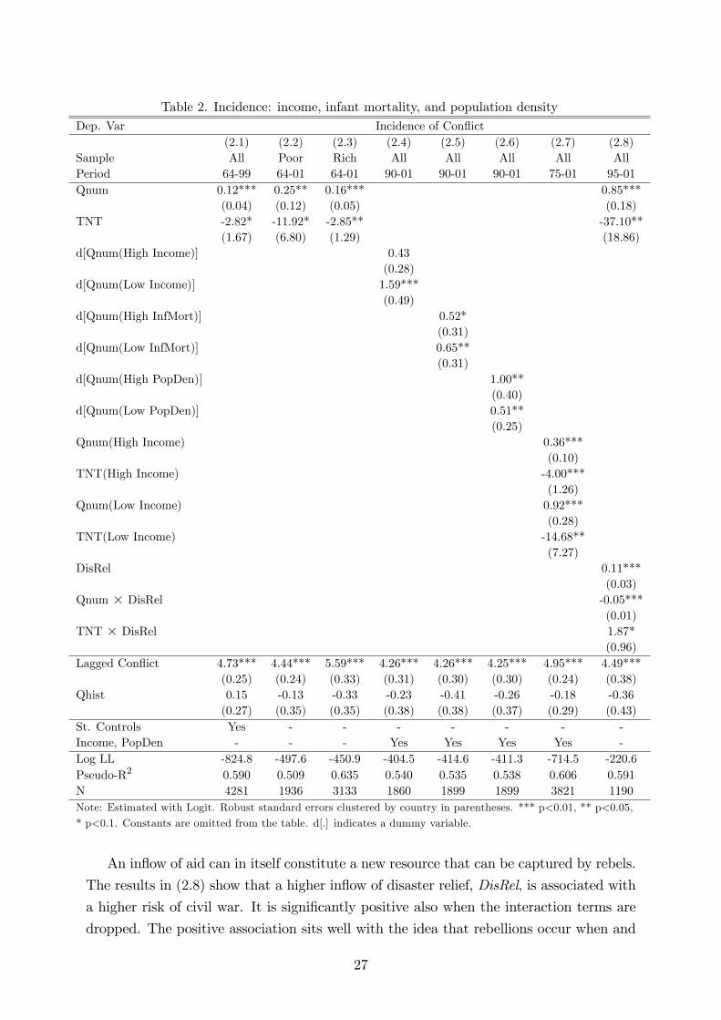
Table 2. Incidence: income, infant mortality, and population densityDep. Var Incidence of Con�ict

(2.1) (2.2) (2.3) (2.4) (2.5) (2.6) (2.7) (2.8)Sample All Poor Rich All All All All AllPeriod 64-99 64-01 64-01 90-01 90-01 90-01 75-01 95-01Qnum 0.12*** 0.25** 0.16*** 0.85***

(0.04) (0.12) (0.05) (0.18)TNT -2.82* -11.92* -2.85** -37.10**

(1.67) (6.80) (1.29) (18.86)d[Qnum(High Income)] 0.43

(0.28)d[Qnum(Low Income)] 1.59***

(0.49)d[Qnum(High InfMort)] 0.52*

(0.31)d[Qnum(Low InfMort)] 0.65**

(0.31)d[Qnum(High PopDen)] 1.00**

(0.40)d[Qnum(Low PopDen)] 0.51**

(0.25)Qnum(High Income) 0.36***

(0.10)TNT(High Income) -4.00***

(1.26)Qnum(Low Income) 0.92***

(0.28)TNT(Low Income) -14.68**

(7.27)DisRel 0.11***

(0.03)Qnum � DisRel -0.05***

(0.01)TNT � DisRel 1.87*

(0.96)Lagged Con�ict 4.73*** 4.44*** 5.59*** 4.26*** 4.26*** 4.25*** 4.95*** 4.49***

(0.25) (0.24) (0.33) (0.31) (0.30) (0.30) (0.24) (0.38)Qhist 0.15 -0.13 -0.33 -0.23 -0.41 -0.26 -0.18 -0.36

(0.27) (0.35) (0.35) (0.38) (0.38) (0.37) (0.29) (0.43)St. Controls Yes - - - - - - -Income, PopDen - - - Yes Yes Yes Yes -Log LL -824.8 -497.6 -450.9 -404.5 -414.6 -411.3 -714.5 -220.6Pseudo-R2 0.590 0.509 0.635 0.540 0.535 0.538 0.606 0.591N 4281 1936 3133 1860 1899 1899 3821 1190Note: Estimated with Logit. Robust standard errors clustered by country in parentheses. *** p<0.01, ** p<0.05,

* p<0.1. Constants are omitted from the table. d[.] indicates a dummy variable.

An in�ow of aid can in itself constitute a new resource that can be captured by rebels.

The results in (2.8) show that a higher in�ow of disaster relief, DisRel, is associated with

a higher risk of civil war. It is signi�cantly positive also when the interaction terms are

dropped. The positive association sits well with the idea that rebellions occur when and

27

where they are materially feasible, but contradicts the idea that rebellions are driven by

political motives.

Both interaction terms in Column 8 are signi�cant. An in�ow of aid thus appears to

reduce both the overall positive e¤ect of earthquakes and the negative e¤ect of potentially

very destructive earthquakes.32 Since an in�ow of aid could dampen the negative e¤ects

on the regular economy and on the rebels�opportunity cost, the �rst result is in line with

the theoretical model. The second result is also in line with the model. To the extent that

more disaster relief means that the future of the economy is less bleak, the interaction

term may capture that the rebels are less discouraged from active rebellion.

Disaster relief should limit su¤ering, especially in the wake of a very strong earthquake.

If rebellions were motivated by human su¤ering or anti-state grievances, we would expect

a negative association between disaster relief and con�ict, and the e¤ect should be the

strongest in the wake of the most serious disasters. The estimates in (2.8) are at odds

with these expectations.

Taken at face value, the estimates nevertheless suggest that aid can be a positive force

in the aftermath of earthquakes unless they are very strong. More research is clearly

needed to uncover the mechanisms behind these e¤ects on the aggregate level and before

the true role of disaster relief in post-disaster situations can be settled.

In sum, the overall e¤ect of earthquakes and the e¤ect of moderate earthquakes is that

violent con�ict becomes more likely. Strong earthquakes work in the opposite direction

and make peace more likely. The e¤ects are stronger in poor areas, but not in areas

where the state is more likely to be weak. These results agree well with the interpretation

that an earthquake can make rebellion more feasible by lowering the opportunity costs of

potential rebels, yet that the potential rebels can lose the economic motivation to rebel

after a strong earthquake.

Consider an alternative explanation for the �ndings �that the state is weakened in

post-disaster situations and that some groups exploit this fact. This explanation does not

�t well with the �nding that the e¤ects may be stronger in areas where the state is likely

to have a stronger presence. Perhaps even more problematic for this explanation are the

negative e¤ects of strong earthquakes. To accept this explanation one must �rst accept

the quite counter-intuitive idea that the state is more weakened by moderate earthquakes

than by strong earthquakes.

Another alternative explanation for the positive e¤ect of moderate earthquakes is that

they make people politically motivated to rebel. Perhaps the ine¢ ciency, incompetence,

or discriminatory policies of a government become apparent in the event of a disaster.

What this explanation does not explain is why people, who should be a aware of such

32There are problems associated with including aid �ows. Fearon (2006) notes that disaster relief oftengoes to countries with an existing civil war. The positive coe¢ cient for DisRel may therefore re�ect thatcountries with an ongoing con�ict receive more disaster relief.

28

shortcomings and obviously already have the �nancial means to rebel, would choose not

to rebel unless there is a natural disaster. Neither does it explain why strong earthquakes

have a negative e¤ect. Surely, the political motivation should not be weaker after a

disaster that results in more su¤ering and more grievances.

At a �rst glance, the negative e¤ects of strong disasters could instead testify that

disasters unite individuals and groups and therefore de-escalate con�icts. The problem

with this interpretation is that most of the destruction is realized directly, or within a

matter of days, and that the threat to ones�safety therefore lies in the past rather than in

the future. This means that cooperation may not be individually rational. Furthermore,

this argument cannot explain why moderate earthquakes have a positive e¤ect on the

risk of con�ict, or why the e¤ects appear to be stronger in poor countries. There is no

rational reason to expect disasters to unite people in poor regions more than they do in

rich regions.

A �nal alternative explanation for the negative e¤ect is that very strong earthquakes

may make rebellion materially infeasible by in some manner destroying the potential

rebel�s capacity to form rebel groups. Suppose for instance that the rebels rely on revenues

coming from the local population. When the population�s normal income-generating

capacity is destroyed, the revenue stream dries up and the rebels cannot �nance their

�ghting and the risk for con�ict will consequently be lower. The data at hand does not

allow a full discrimination between this story and the argument advocated in the model,

but we fail to see how this story can explain the fact that moderate earthquakes increase

the risk of con�ict. If the link to con�ict is that a disaster implies less revenues for the

rebels, then should not also weaker earthquakes be followed by a lower risk of con�ict?

The results presented so far do not answer the question of whether moderate (strong)

earthquakes make the onset of new con�icts more (less) likely or make the termination

of ongoing con�icts less (more) likely. As such, they are silent on the issue of whether

natural disasters can defuse tensions, a belief held by several relief organizations and

policy makers. To make an investigation of this issue possible, the following two sections

separate the analysis into the e¤ects on the onset and the e¤ects on the termination of

con�ict.

6.2 Onset

A country runs a signi�cantly higher risk of witnessing a new civil war if there was an

earthquake registered in the country that same year; see the �rst column in Table 3.

Qhist is mostly negative, which indicates that a more recent earthquake is associated

with a higher con�ict risk, but the estimates are not robust. Nel and Righarts (2008)

�nd that the Brevity of Peace has no signi�cant e¤ect when the dependent variable is

onset of con�ict with less than 1,000 deaths, and this is what we observe in most of our

29

speci�cations as well.33

The destructive potential of strong earthquakes has a negative e¤ect both when in-

cluded separately, as in Column 2, and when included together with the number of earth-

quakes, as in Column 3. In results not shown, the square of Qnum was added to speci�-

cation (3.3), and was not signi�cant. The e¤ect on the coe¢ cient for TNT was marginal

(from -23.1 to -23.8): hence what TNT is picking up is not some form of diminishing

marginal e¤ect of having many earthquakes.34

The probability of onset in the sample used for (3.3) is 2.1 percent if there are no

earthquakes. Consider the same stylized scenarios as above. The estimated coe¢ cients in

(3.3) imply that the probability of onset in the �rst scenario, with four M6.0 earthquakes,

is 4.5 percent. The implied probability of onset in the second scenario, with one M7.5

and three M6.0 earthquakes, is a mere 0.1 percent. Again, this is lower than if there was

no earthquake.

Nel and Righarts (2008) �nd that the risk of onset was twice as high in countries that

experienced an earthquake or a volcanic eruption. In results not shown we used a dummy

to indicate whether there was an earthquake. The implied risk of onset was 3.0 percent if

there was an earthquake, and 2.1 percent if there was not, but the p-value of the estimate

was 0.11.

The estimates forQnum and TNT are signi�cant both when the ten Standard Controls

are added and when unobserved country characteristics and year dummies are controlled

for. Compare this with (1.4) where Qnum had no signi�cant e¤ect on the Incidence of

con�ict in a �xed e¤ects estimation. Evidently, while TNT has a quite robust negative

e¤ect on both the occurrence and onset of con�ict, the e¤ect of Qnum seems to be more

connected to the onset than to the incidence of con�ict. As shown in the next section,

this interesting result can partly be explained by the fact that strong earthquakes have a

more robust e¤ect on the termination of con�ict than moderate earthquakes do. However,

it should be noted that the e¤ect of Qnum even on Onset is not entirely robust to the

exclusion of potential outliers, while TNT is.35

33A negative coe¢ cient for Brevity of Peace, which we �nd in some of our regressions, means that onsetis actually more likely in countries with a longer tradition of peace. This result is somewhat of a puzzle,and would be interesting to investigate further.34Speci�cations (3.3) and (1.3) were estimated with both Rare Event Logit (ReLogit) and OLS, and

Qnum and TNT remain signi�cant. Nel and Righarts (2008) use ReLogit, which they argue providesbetter estimates when the dependent variable represents �rare events.� Fearon and Laitin (2003) andCollier and Hoe er (2004) report no important di¤erences when using ReLogit. The qualitative resultsare also the same when the higher threshold of 1,000 battle deaths is used to code the onset variable. Analternative TNT measure was created, where all earthquakes with magnitude above M7.0 were treatedas having M7.0. In results not shown, the estimate for this alternative TNT measure, when used in (3.3)and (1.3), also showed a negative and signi�cant e¤ect of TNT. Also in results not shown, Qnum wasreplaced by the log of (1+Qnum) and TNT by the log of (1+TNT ), both in (1.3) and in (3.3). Bothvariables retained their signs and were highly signi�cant.35TNT remains signi�cant when we drop potential outliers from (3.3) as described in Footnote 26.

Qnum is signi�cant when observations are dropped based on high leverage, but not when dropped basedon standardized or deviance residuals.

30

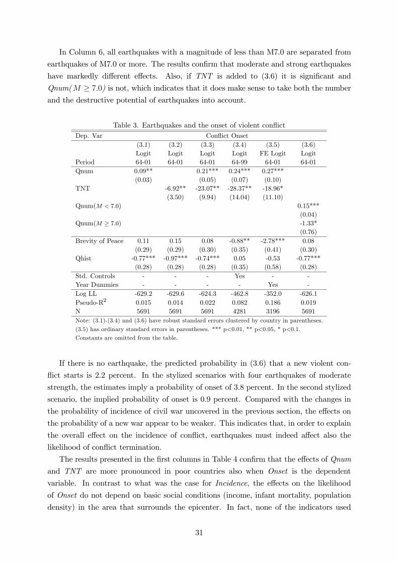
In Column 6, all earthquakes with a magnitude of less than M7.0 are separated from

earthquakes of M7.0 or more. The results con�rm that moderate and strong earthquakes

have markedly di¤erent e¤ects. Also, if TNT is added to (3.6) it is signi�cant and

Qnum(M � 7:0) is not, which indicates that it does make sense to take both the numberand the destructive potential of earthquakes into account.

Table 3. Earthquakes and the onset of violent con�ictDep. Var Con�ict Onset

(3.1) (3.2) (3.3) (3.4) (3.5) (3.6)Logit Logit Logit Logit FE Logit Logit

Period 64-01 64-01 64-01 64-99 64-01 64-01Qnum 0.09** 0.21*** 0.24*** 0.27***

(0.03) (0.05) (0.07) (0.10)TNT -6.92** -23.07** -28.37** -18.96*

(3.50) (9.94) (14.04) (11.10)Qnum(M < 7:0) 0.15***

(0.04)Qnum(M � 7:0) -1.33*

(0.76)Brevity of Peace 0.11 0.15 0.08 -0.88** -2.78*** 0.08

(0.29) (0.29) (0.30) (0.35) (0.41) (0.30)Qhist -0.77*** -0.97*** -0.74*** 0.05 -0.53 -0.77***

(0.28) (0.28) (0.28) (0.35) (0.58) (0.28)Std. Controls - - - Yes - -Year Dummies - - - - Yes -Log LL -629.2 -629.6 -624.3 -462.8 -352.0 -626.1Pseudo-R2 0.015 0.014 0.022 0.082 0.186 0.019N 5691 5691 5691 4281 3196 5691Note: (3.1)-(3.4) and (3.6) have robust standard errors clustered by country in parentheses.

(3.5) has ordinary standard errors in parentheses. *** p<0.01, ** p<0.05, * p<0.1.

Constants are omitted from the table.

If there is no earthquake, the predicted probability in (3.6) that a new violent con-

�ict starts is 2.2 percent. In the stylized scenarios with four earthquakes of moderate

strength, the estimates imply a probability of onset of 3.8 percent. In the second stylized

scenario, the implied probability of onset is 0.9 percent. Compared with the changes in

the probability of incidence of civil war uncovered in the previous section, the e¤ects on

the probability of a new war appear to be weaker. This indicates that, in order to explain

the overall e¤ect on the incidence of con�ict, earthquakes must indeed a¤ect also the

likelihood of con�ict termination.

The results presented in the �rst columns in Table 4 con�rm that the e¤ects of Qnum

and TNT are more pronounced in poor countries also when Onset is the dependent

variable. In contrast to what was the case for Incidence, the e¤ects on the likelihood

of Onset do not depend on basic social conditions (income, infant mortality, population

density) in the area that surrounds the epicenter. In fact, none of the indicators used

31

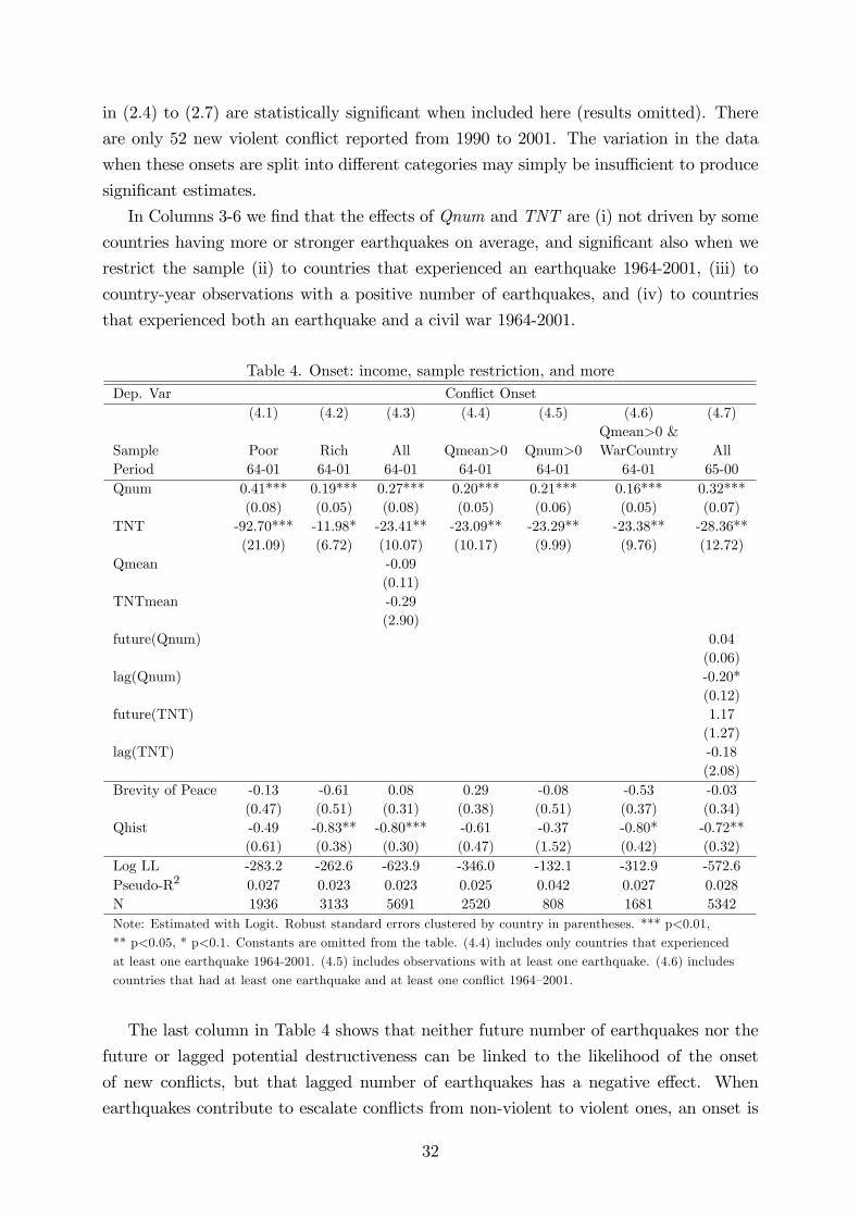
in (2.4) to (2.7) are statistically signi�cant when included here (results omitted). There

are only 52 new violent con�ict reported from 1990 to 2001. The variation in the data

when these onsets are split into di¤erent categories may simply be insu¢ cient to produce

signi�cant estimates.

In Columns 3-6 we �nd that the e¤ects of Qnum and TNT are (i) not driven by some

countries having more or stronger earthquakes on average, and signi�cant also when we

restrict the sample (ii) to countries that experienced an earthquake 1964-2001, (iii) to

country-year observations with a positive number of earthquakes, and (iv) to countries

that experienced both an earthquake and a civil war 1964-2001.

Table 4. Onset: income, sample restriction, and moreDep. Var Con�ict Onset

(4.1) (4.2) (4.3) (4.4) (4.5) (4.6) (4.7)Qmean>0 &

Sample Poor Rich All Qmean>0 Qnum>0 WarCountry AllPeriod 64-01 64-01 64-01 64-01 64-01 64-01 65-00Qnum 0.41*** 0.19*** 0.27*** 0.20*** 0.21*** 0.16*** 0.32***

(0.08) (0.05) (0.08) (0.05) (0.06) (0.05) (0.07)TNT -92.70*** -11.98* -23.41** -23.09** -23.29** -23.38** -28.36**

(21.09) (6.72) (10.07) (10.17) (9.99) (9.76) (12.72)Qmean -0.09

(0.11)TNTmean -0.29

(2.90)future(Qnum) 0.04

(0.06)lag(Qnum) -0.20*

(0.12)future(TNT) 1.17

(1.27)lag(TNT) -0.18

(2.08)Brevity of Peace -0.13 -0.61 0.08 0.29 -0.08 -0.53 -0.03

(0.47) (0.51) (0.31) (0.38) (0.51) (0.37) (0.34)Qhist -0.49 -0.83** -0.80*** -0.61 -0.37 -0.80* -0.72**

(0.61) (0.38) (0.30) (0.47) (1.52) (0.42) (0.32)Log LL -283.2 -262.6 -623.9 -346.0 -132.1 -312.9 -572.6Pseudo-R2 0.027 0.023 0.023 0.025 0.042 0.027 0.028N 1936 3133 5691 2520 808 1681 5342Note: Estimated with Logit. Robust standard errors clustered by country in parentheses. *** p<0.01,

** p<0.05, * p<0.1. Constants are omitted from the table. (4.4) includes only countries that experienced

at least one earthquake 1964-2001. (4.5) includes observations with at least one earthquake. (4.6) includes

countries that had at least one earthquake and at least one con�ict 1964�2001.

The last column in Table 4 shows that neither future number of earthquakes nor the

future or lagged potential destructiveness can be linked to the likelihood of the onset

of new con�icts, but that lagged number of earthquakes has a negative e¤ect. When

earthquakes contribute to escalate con�icts from non-violent to violent ones, an onset is

32

recorded. These con�icts are not counted as onsets in the following year, which could

explain the negative e¤ect of lagged number of earthquakes.

A natural, yet important, conclusion from this subsection is that a central reason

for the association between su¤ering from earthquakes and experiencing a violent civil

con�ict is simply that earthquakes a¤ect the probability that violent con�icts are started.

Whether earthquakes are also linked to con�ict termination is investigated in the next

subsection.

6.3 Termination

The theoretical model is not designed to provide clear predictions as to why con�icts

eventually end. As a �rst approximation, we hypothesize that the e¤ects of disaster

destruction � on the likelihood of termination are roughly the reverse of its e¤ects on the

likelihood of onset or incidence: moderate earthquakes should make the termination of

con�ict less likely and strong earthquakes should make the termination of con�ict more

likely.

The results presented in Table 5 show that earthquakes in�uence the probability that

civil wars are ended. The sample used here consists of countries that had an active con�ict

in the previous year. It is therefore considerably smaller than the samples used when we

focused on Incidence or Onset. That Brevity of Con�ict is signi�cant and positive in

most of our speci�cations indicates that the termination of con�ict is indeed more likely

if the last year of peace is closer in time.

Speci�cation (5.1) shows that Qnum and TNT have the predicted signs, but their

e¤ects on the likelihood of Termination are not signi�cant. The results are the same if

they are included separately.

The second column separates moderate earthquakes from strong ones, and now we

see that strong earthquakes are positively associated with the likelihood of termination.

The simplicity of these dummies may explain the di¤erent results in (5.2) as compared

to (5.1). The e¤ect of the dummy for moderate earthquakes has the predicted sign but

is not signi�cant. In fact, none of the indicators for moderate earthquakes ever enters

signi�cantly in the full sample unless conditions around the epicenter are considered.

Hence, the dynamics that determine the termination of con�ict only partly mirror those

that determine the onset of con�ict.36

In Column 3 we include only strong earthquakes and use the full 1947-2001 period to

obtain a larger sample. This change hardly a¤ects the estimate for strong earthquakes.

Strong earthquakes are, as we have previously stressed, quite rare. Therefore, it is a com-

36The qualitative results in (5.2) are the same when ReLogit is used and if year dummies are added,but they are not robust to Fixed E¤ects. Moderate earthquakes have a signi�cantly negative e¤ect andstrong earthquakes a signi�cantly positive e¤ect when the Standard Controls are added to (5.2). Thisappears to be a result of the smaller sample (202 observations less due to missing data).

33

fort that the results in (5.3) are not driven by a few excessively in�uential observations.37

The predicted probability of termination in (5.3) if there is no strong earthquake is 20.0

percent. The likelihood of Termination jumps to 35.3 percent if the country experiences

an earthquake with a magnitude of 7 or more. Apparently, the magnitude of the e¤ect

is substantial and the result supports the view that natural disasters can contribute to

de-escalate con�icts.

When we split the sample into poor and rich observations, we �nd that experiencing

a strong earthquake makes the termination of con�ict more likely and experiencing a

moderate earthquakes makes the termination of con�ict less likely only in the sample

where the income level is low. The results in Column 6 con�rm that the overall e¤ects of

earthquakes are more pronounced in poor regions. The e¤ect of an earthquake that strikes

a poor region is that it makes the termination of con�icts less likely, while an earthquake

that strikes a rich area has no such e¤ect. The indicators for strong earthquakes in rich

or poor regions are, however, far from signi�cant (results omitted).

Why is the e¤ect of strong earthquakes in poor regions not at all signi�cant when the

e¤ect of strong earthquakes in poor countries is positive and highly signi�cant? It could

be a matter of a small sample and lack of variation in the data. When there already

are fairly few strong earthquakes, it matters that some are dropped because of missing

data on income or population density on the regional level. As the sample is restricted

to 1990-2001 and to countries that had an active con�ict in the previous year, there may

simply be insu¢ cient variation in the data to identify the e¤ects of strong earthquakes.38

It could also be that the income level in the area that immediately surrounds the

epicenter is a very noisy measure of the directly a¤ected people�s income level. Instead,

data on the national level may better capture the average income level in the whole

a¤ected area. A third explanation for the lack of signi�cance is that the local income

level is of minor importance when it comes to the economic motives for rebellion, but

that the national income level is not. This would be the case if the rebels are �ghting to

take control of the whole country rather than only part of it. The data at hand does not

allow us to discriminate between these alternative explanations.

The results in (5.7) show that strong earthquakes make con�ict termination more

likely only when a region with a population density of between 10 and 50 persons per

km2 is struck rather than an area with more than of 50 persons per km2. Fewer people

should be directly a¤ected in less densely populated areas, hence the results show that

what matters most here is not the number of people potentially a¤ected, but rather that

people in less densely populated areas are more likely to become isolated and that the

state probably has a weaker presence in these areas.

37The indicator for strong earthquakes remains highly signi�cant when we drop outliers as describedin Footnote 26.38The in�ow of disaster relief has been included and interacted with the indicators for earthquakes.

The results are not signi�cant in any direction, quite possibly because the sample becomes very small.

34

The samples used in this subsection, and especially the samples used in Columns 4-7

are quite small; hence we should not overinterpret the results. Nevertheless, there are

indications that a country with an ongoing civil war is more likely to become peaceful if

it experiences a strong earthquake, and especially if it is a poor country or if the area

surrounding the epicenter has a relatively low population density. On the other hand, the

overall e¤ects of (all) earthquakes with epicenters in poor areas may be that termination

becomes less likely, i.e., they may instead prolong con�icts.

Table 5. Earthquakes and the termination of con�ictDep. Var Termination of Con�ict

(5.1) (5.2) (5.3) (5.4) (5.5) (5.6) (5.7)Sample All All All Poor Rich All AllPeriod 64-01 64-01 47-01 64-01 64-01 90-01 90-01Qnum -0.01

(0.05)TNT 1.91

(1.47)d[Qnum(M < 7:0)] -0.33 -0.98** -0.10

(0.25) (0.49) (0.29)d[Qnum(M � 7:0)] 0.83*** 0.78*** 1.06*** 0.69

(0.30) (0.25) (0.40) (0.47)d[Qnum (High Income)] 0.08

(0.41)d[Qnum (Low Income)] -0.97**

(0.44)

dhQnum

�M � 7:0

High PopDen

�i-1.53

(1.07)

dhQnum

�M � 7:0

Low PopDen

�i1.83***

(0.71)Brevity of Con�ict 1.98*** 1.94*** 2.08*** 1.76*** 2.82*** 2.33*** 2.34***

(0.36) (0.35) (0.36) (0.51) (0.43) (0.50) (0.49)Qhist -0.18 -0.29 -0.03 -0.27 -0.24 -0.53 -0.32

(0.25) (0.25) (0.23) (0.42) (0.33) (0.48) (0.40)Income, PopDen - - - - - Yes YesLog LL -460.6 -459.1 -534.3 -213.6 -175.2 -188.4 -188.8Pseudo-R2 0.057 0.060 0.067 0.056 0.118 0.098 0.099N 954 954 1077 417 413 348 350Note: Estimated with Logit. Robust standard errors clustered by country in parentheses. *** p<0.01,

** p<0.05, * p<0.1. Constants are omitted from the table. d[.] indicates a dummy variable.

In sum, earthquakes a¤ect both the onset and termination of con�icts and as a result

the incidence of con�ict. Furthermore, the magnitude of an earthquake is of fundamental

importance, as are the social conditions in the area surrounding the epicenter. Moderate

earthquakes increase the likelihood that con�icts start and may reduce the likelihood that

con�icts end. Strong earthquakes are associated with a lower likelihood that con�icts are

started and with a higher likelihood that con�icts are ended, and these e¤ects tend to be

35

stronger in poor countries, or when the epicenter is found in a region with a relatively low

population density.


While the empirical literature has tended to �nd that natural disasters increase the risk

of con�ict, the intuition among some relief organizations is that natural disasters can

contribute to reduce tensions and in the end reduce the risk of violent con�ict. This

paper shows that there is some truth to both of these stories and that the outcome in

each case is determined by the severity of the disaster and the basic social conditions in

the directly a¤ected area.

We develop a theoretical model of natural disasters and violent con�ict. The model

shows how natural disasters can, via the destruction of physical capital, a¤ect both the

costs and revenues of rebellion. The moderate destruction caused by moderate natural

disasters can make rebellion feasible by lowering the opportunity cost of potential recruits.

More intense destruction means that the material payo¤ in the event of a victorious

rebellion is lower. Taken together, the model predicts that violent con�ict should be more

likely after moderate disasters and less likely after very strong disasters, and that both

these e¤ects should be more pronounced in poor areas.

The empirical analysis employs an exhaustive dataset on earthquakes. We can estab-

lish that the general e¤ect of moderate earthquakes is that they make new civil wars more

likely, and maybe the termination of ongoing civil wars less likely. The e¤ects of stronger

earthquakes are the opposite, i.e., they make new civil wars less likely and termination of

ongoing civil wars more likely. The �ndings are the �rst to link a fully exogenous measure

of the severity of a potential natural disaster, namely an approximation of the seismic

energy released by earthquakes, to the risk of civil war.

Most earthquakes are of moderate strength wherefore the overall e¤ect is that violent

con�icts are started and that ongoing con�icts are less likely to be terminated. The

combined e¤ect explains earlier �ndings of a generally positive e¤ect on the incidence of

violent con�ict. The e¤ects, both the con�ict-promoting e¤ect of moderate earthquakes

and the con�ict-defusing e¤ect of stronger earthquakes, are more pronounced in poor

areas and areas with a weak state presence. Accordingly, the results are consistent with

the theoretical model.

We can now conclude that both the tradition claiming that natural disasters can cause

violent con�ict and the tradition claiming that natural disasters can end violent con�ict

hold pieces of the truth. As such, the present analysis constitutes the �rst systematic

study to establish that natural disasters can give the impetus needed to end existing

con�icts and prevent new violent con�icts from emerging.

36

ReferencesAlbala-Bertrand, J.M. (1993) Political Economy of Large Natural Disasters: With Special

Reference to Developing Countries, Oxford: Clarendon Press.

Anbarci, N., M. Escaleras, and C.A. Register (2005) �Earthquake fatalities: the interactionof nature and political economy�Journal of Public Economics, 89:1907�33.

Barnett, J. and W.N. Adger (2007) �Climate change, human security and violent con�ict�Political Geography, 26:639-55.

Bhavnani, R. (2006) �Natural Disaster Con�icts�mimeo, Harvard University.

Blattman, C. and E. Miguel (2009) �Civil War�NBER Working Paper 14801.

Bolt, B.A. (2006) Earthquakes (5th ed.), New York: W.H. Freeman and Company.

Brancati, D. (2007) �Political Aftershocks: The Impact of Earthquakes on Intrastate Con-�ict�Journal of Con�ict Resolution, 51(5):715-43.

Brunnschweiler, C. and E. Bulte (2008a) �Linking Natural Resources to Slow Growth andMore Con�ict�Science, 320(5876):616-7.

Brunnschweiler, C. and E. Bulte (2008b) �Natural Resources and Violent Con�ict: ResourceAbundance, Dependence and the Onset of Civil Wars�CER-ETH Zurich Working PaperNo. 08/78.

Centennial Earthquake Catalog (2008), available online at http://earthquake.usgs.gov/research/data/centennial.php.

Collier, P. (2000) �Rebellion as a Quasi-Criminal Activity�Journal of Con�ict Resolution,44(6):839-53.

Collier, P. and A. Hoe er (2004) �Greed and Grievance in Civil War�Oxford EconomicPapers, 56(4):563-95.

Collier, P. and A. Hoe er (2005) �Resource Rents, Governance, and Con�ict� Journal ofCon�ict Resolution, 49(4):625-33.

Collier, P., A. Hoe er, and M. Söderbom (2004) �On the Duration of Civil War�Journalof Peace Research, 41(3):253-73.

Collier, P. A. Hoe er, and D. Rohner (2009) �Beyond greed and grievance: feasibility andcivil war�Oxford Economic Papers, 61:1-27.

Dixon, J. (2009) �Emerging Consensus: Results from the Second Wave of Statistical Studieson Civil War Termination�Civil Wars, 11(2):121-36.

Drury, A.C. and R.S. Olson (1998) �Disaster and Political Unrest: An Empirical Investiga-tion�Journal of Contingencies and Crisis Management, 6(3):153-61.

EDIT (2009) The European Distributed Institute of Taxonomy, available online at http://edit.csic.es/.

EM-DAT (2008) The CRED International Disaster Database, Université Catholique de Lou-vain, Belgium.

Engdahl, E.R. and A. Villaseñor (2002) �Global Seismicity: 1900�1999� in InternationalHandbook of Earthquake and Engineering Seismology (eds. Lee, W.H.K., H. Kanamori,P.C. Jennings, and C. Kisslinger), Part A, Ch. 41, 665�90, Academic Press.

Fearon, J.D. (2004) �Why Do Some Civil Wars Last So Much Longer than Others?�Journalof Peace Research, 41(3):275-301.

Fearon, J.D. (2005) �Primary Commodity Exports and Civil War�Journal of Con�ict Res-olution, 49(4):483-507.

Fearon, J.D. (2006) �The Rise of Emergency Relief Aid�mimeo, Stanford University.

37

Fearon, J.D. and D.D. Laitin (2003) �Ethnicity, Insurgency, and Civil War�American Po-litical Science Review, 97(1):75-90.

Fearon, J.D. and D.D. Laitin (2007) �Civil War termination�mimeo, Stanford University.

G-Econ (2008) Geographically based Economic data, available online at http://gecon.yale.edu/.

Gallup, J.L., J.D. Sachs, and A.D. Mellinger (1999) �Geography and Economic Develop-ment�International Regional Science Review, 22(2):179-232.

Gar�nkel, M.R. and S. Skaperdas (2007) �Economics of Con�ict: An Overview�in Handbookof Defense Economics (eds. Sandler, T. and K. Hartley), Vol. 2, Ch. 3, p.649-710.

Gleditsch, K.S., and M.D. Ward (1999) �Interstate System Membership: A Revised List ofthe Independent States since 1816�International Interactions, 25:393�413.

Global Poverty Mapping Project (2009), available online at http://sedac.ciesin.columbia.edu/povmap/.

Grossman, H.I. and M. Kim (1995) �Swords or plowshares? A theory of the security ofclaims to property�Journal of Political Economy, 103(6):1275-88.

Grossman, H.I. (1999) �Kleptocracy and revolutions�Oxford Economic Papers, 51:267-83.

Hegre, H., T. Ellingsen, S. Gates, and N. P. Gleditsch (2001) �Toward a Democratic CivilPeace? Democracy, Political Change, and Civil War, 1816-1992� American PoliticalScience Review, 95(1):33-48.

Hegre, H. (2004) �The Duration and Termination of Civil War�Journal of Peace Research,41(3):243-52.

Hegre, H. and N. Sambanis (2006) �Sensitivity Analysis of Empirical Results on Civil WarOnset�Journal of Con�ict Resolution, 50(4):508-35.

Heston, A., R. Summers, and B. Aten (2009), Penn World Table Version 6.2, Center forInternational Comparisons of Production, Income and Prices at the University of Penn-sylvania, available online at http://pwt.econ.upenn.edu/.

Homer-Dixon, T. (1994) �Environmental Scarcities and Violent Con�ict: Evidence fromCases�International Security, 19(1):5-40.

Horwich, G. (2000) �Economic Lessons of the Kobe Earthquake�Economic Developmentand Cultural Change, 48:521-42.

Humpreys, M. (2005) �Natural Resources, Con�ict, and Con�ict Resolution: Uncoveringthe Mechanisms�Journal of Con�ict Resolution, 49(4):508-37.

Kahl, C.H. (2006) States, Scarcity, and Civil Strife in the Developing World, Princeton:Princeton University Press.

Kahn, M.E. (2004) �The death toll from natural disasters: the role of income, geography,and institutions�Review of Economics and Statistics, 87(2):271-84.

Kelman, I. (2003) �Beyond disaster, beyond diplomacy� in Natural disasters and develop-ment in a globalizing world (ed. M. Pelling), New York: Routledge.

Kenny, C. (2009) �Why Do People Die in Earthquakes? The Costs, Bene�ts and Institu-tions of Disaster Risk Reduction in Developing Countries�World Bank Policy ResearchWorking Paper 4823.

Kreutz, J. (2010) �How and When Armed Con�icts End: Introducing the UCDP Con�ictTermination Dataset�Journal of Peace Research, forthcoming.

La Porta, R., F. Lopez-de-Silanes, A. Shleifer, and R. Vishny (1999) �The Quality of Gov-ernment�Journal of Law, Economics, & Organizations, 15(1):222-79.

38

Le Billon, P. and A. Waizenegger (2007) �Peace in the wake of disaster? Secessionist con�ictsand the 2004 Indian Ocean tsunami�Transactions of the Institute of British Geographers,32(3):411-27.

Lujala, P. (2009) �Deadly Combat over Natural Resources: Gems, Petroleum, Drugs, andthe Severity of Armed Civil Con�ict�Journal of Con�ict Resolution, 53(1):50-71.

Miguel, E., S. Satyanath, and E. Sergenti (2004) �Economic Shocks and Civil Con�ict: AnInstrumental Variables Approach�Journal of Political Economy, 112(4):725-53.

Nel, P. and M. Righarts (2008) �Natural Disasters and the Risk of Violent Civil Con�ict�International Studies Quarterly, 52(1):159-85.

Nordås, R. and N.P. Gleditsch (2007) �Climate change and con�ict�Political Geography,26:627-38.

Noy, I. (2009) �The macroeconomic consequences of disasters�Journal of Development Eco-nomics, 88:221�31.

OECD (2004) Large-Scale Disasters: Lessons Learned, Paris: OECD.

OECD (2009) OECD.Stat, available online at http://stats.oecd.org/.

Olson, R.S. and A.C. Drury (1997) �Un-therapeutic communities: a cross-national analysisof post-disaster political unrest�International Journal of Mass Emergencies and Disas-ters, 15:221�38.

Olsson, O. (2007) �Con�ict Diamonds�Journal of Development Economics, 82:267-86.

PRIO/Uppsala (2008) �UCDP/PRIO intrastate con�ict onset dataset, 1946-2006,�availableonline at http://new.prio.no/CSCW-Datasets/.

Red Cross (2007) World Disaster Report, Geneva: International Federation of the RedCross/Red Crescent Society.

Reuveny, R. (2007) �Climate change-induced migration and violent con�ict�Political Geog-raphy, 26(6):656-73.

Ross, M.L. (2004) �What Do We Know about Natural Resources and Civil War?�Journalof Peace Research, 41(3):337-56.

de Rouen, K.R and D. Sobek (2004) �The Dynamics of Civil War Duration and Outcome�Journal of Peace Research, 41(3):303-20.

Skaperdas, S. (1996) �Contest success functions�Economic Theory, 7:283-90.

Strömberg, D. (2007) �Natural Disasters , Economic Development, and Humanitarian Aid�Journal of Economic Perspectives, 21(3):199-222.


Toya, H. and M. Skidmore (2007) �Economic Development and the impacts of naturaldisasters�Economic Letters, 94:20-5.

UCDP (2008) �UCDP Con�ict Termination dataset, Version 2.1 �September 4 2008,�avail-able online at http://www.pcr.uu.se/research/UCDP/.

UNDP (2004) Reducing Disaster Risk: A Challenge for Development, New York: UNDP.

Urdal, H. (2005) �People vs Malthus: Population Pressure, Environmental Degradation, andArmed Con�ict Revisited�Journal of Peace Research 42(4):417-34.

Urdal, H. (2006) �A Clash of Generations? Youth Bulges and Political Violence� Interna-tional Studies Quarterly, 50(3):607-29.

USGS (2008) United States Geological Survey, available online at http://earthquake.usgs.gov/.

WBGU (2008) Climate Change as a Security Risk, available online at http://www.wbgu.de/wbgu_jg2007_engl.html.

39

Appendix A

Proof of Proposition 1

If (4) does not hold, the choices of I and S are trivial as it implies that V = 0. The cost

of hiring rebel �ghters cannot be motivated when future incomes are zero, implying that

I = 0. Expecting I = 0, Q sets S = 0.


The rebel resource constraint (RRC) is slack when Irrc > I�, or when � > �. The range

of � that is compatible with the conditions for Proposition 2 is therefore � < � < ~� .

There is �ghting, I > 0, if S� < S, and this is the case when � > 12, i.e., when the rebels

are su¢ ciently e¢ cient �ghters.

When (4) and (RRC) are slack, the tax rate is t = A(1��)K�YA(1��)K , the size of the rebel

army is I� = A(1��)K�Y2�A(1��)K

�1� 1

2�

�, and the size of the government army is S� = A(1��)K�Y

4�A(1��)K .

Also, (RRC) will not become binding at higher � if it stops to bind at �. The reason is

that dI�

d�< 0 while dIrrc

d�> 0, as discussed below. This means that Irrc will not fall as �

increases, but I� will. This means that if Irrc > I�, it will stay that way when � increases,

and (RRC) will remain slack. The dynamics of I� and p are evident from straightforward

di¤erentiation.


The level of destruction compatible with the outcome in Proposition 3 is � � �. When

� < 1=2, the optimal I is I� = 0. For (RRC) to bind, which requires that (5) holds, I� > 0

is needed, i.e., S� < S, or � > 1=2. J will set I = Irrc under these conditions. On the

one hand, when (RRC) binds, I > Irrc is not possible, wherefore any S < Srrc will still

induce J to set I = Irrc. On the other hand, any S > Srrc means that J sets I < Irrc ,

but as this implies that (RRC) is slack, J simply sets I = I�.

Importantly, as long as the S that Q sets implies a binding (RRC), Q can treat I as

�xed at Irrc. This is the case since when Q observes that the rebel resource constraint will

be slack, it determines the optimal size S foreseeing two e¤ects that the size of its army

has on the probability that it wins the war. There is a direct e¤ect in that a higher S

40

implies a higher p, but there is also an indirect e¤ect as a higher S has a deterring e¤ect

on the I� that J sets. Provided that the S that Q sets is in the range where it implies

an optimal I� > Irrc, it turns out that Q only has to consider the direct e¤ect of S on p.

This means that whenever the government foresees that the rebel resource constraint will

be strictly binding, it will set S < S�, and the rebels will respond by setting I as high as

possible.

Hence, if � > 1=2 and J wants to set I� > 0 but (RRC) binds, J sets Irrc. Foreseeing

this, rather than setting S� as if (RRC) were slack, the government chooses S to maximize

its expected net wealth as in (3). Given that I = Irrc, the probability of a government

victory is p = S= (S + �Irrc) with @p=@S = (�Irrc) = (S + �Irrc)2. Restricting S to be

non-negative, the optimal size of the government army is Srrc =p�Irrct� �Irrc.

In sum, J cannot set I > Irrc and will not set I < Irrc. Given Srrc =p�Irrct� �Irrc,

any I < Irrc gives J a lower expected utility. This is clear as it is unambiguously the

case that J(I = Irrc � b j Srrc) < J(I = Irrc j Srrc) for all positive b, given that � < 1.

Rationally, J responds by setting Irrc.

This Irrc also satis�es the rebel incentive constraint (1), i.e. that Irrc � (1� p) t.

With I = Irrc and S = Srrc, (1) can be rewritten as Irrc < �t, which demands that

Rj < � (A (1� �)K � Y ), or that � < �� = 1 � 1AK

�Rj�+ Y

�. When (RRC) binds, and

therefore also (5), this will always be the case. Note also that � < ��, i.e., that the level

of destruction where (RRC) stops to bind is lower than the level where (1) binds. This

implies that (RRC) is slack at all � > ��, and that at such �, the relevant outcome is

described in Propositions 1 or 2.

When � > 1=2 and (RRC) binds, the size of the rebel army becomes Irrc =Rj

A(1��)K

and the size of the government army becomes Srrc =q

�Rj(A(1��)K�Y )(A(1��)K)2 � �Rj

A(1��)K . The

dynamics of Irrc and p are evident from straightforward di¤erentiation.

41

Appendix B

Basic facts about earthquakes

Table B1. Basic facts about earthquakesPanel A Magnitude Annual average

3-3.9 1300004-4.9 130005-5.9 13196-6.9 1347-7.9 17>8 1

Approximate TNT forPanel B Magnitude Seismic Energy Yield Example

3.0 32 (metric) tons4.0 1 kiloton Small Atomic Bomb5.0 32 kilotons Nagasaki Atomic Bomb6.0 1 megaton7.0 32 megatons Largest Hydrogen Bomb; Kobe, 19958.0 1 gigaton San Francisco, 19069.0 32 gigatons Chile, 1960

Panel C Magnitude Typical damage<3.5 Generally not felt, but recorded.3.5-5.4 Often felt, but rarely causes damage.<6.0 At most slight damage to well-designed buildings.

Can cause major damage topoorly constructed buildings over small regions.

6.1-6.9 Can be destructive in areas up to about100 kilometers across where people live.

7.0-7.9 Can cause serious damage over larger areas.>8 Can cause serious damage in areas several

hundred kilometers across.Note: The source is USGS (2008).

Earthquakes and the number of disaster victims

The results presented in Table B2 indicate that we are correct in assuming that stronger

earthquakes have more serious direct consequences. The data on earthquakes is taken

from the Centennial Earthquakes Catalog (2008). The seriousness of disasters is captured

by the variable Disaster Victims, which we de�ne as the log of the number of dead,

injured, or homeless due to natural disasters, as reported in the EM-DAT database. The

data was retrieved from Nel and Righarts (2008). All speci�cations include a constant,

Qhist, year dummies, and population size. The sample consists of observations with a

disaster recorded in the EM-DAT database.39

39Observations for which no natural disaster is reported in the EM-DAT have zero Disaster Victims.We obtain the same qualitative results as in Table B2 when we include these observations in the sample

42

The �rst four columns are estimated with linear Fixed E¤ects. Qnum(M < 7:0)

indicates the number of moderate earthquakes, i.e., those with a magnitude of less than

M7.0. Strong earthquakes, i.e., those with a magnitude of M7.0 or more are included as

Qnum(M � 7:0). In the table, it is evident that both moderate and strong earthquakes

are associated with a larger number of disaster victims, and that the e¤ects of strong

earthquakes are more serious. That TNT is positive and signi�cant when Qnum is held

constant shows that it is not just the number of earthquakes that matters but also their

size, i.e., more people die, are injured, or become homeless in earthquakes with a higher

destructive potential, as approximated by TNT.

Table B2. Earthquakes and Disaster VictimsDep. Var. Disaster Victims

(B2.1) (B2.2) (B2.3) (B2.4)Sample All All All Qnum>0Period 64-00 64-00 64-99 64-00Qnum(M < 7:0) 0.20***

(0.07)Qnum(M � 7:0) 1.32***

(0.30)Qnum 0.24*** 0.22*** 0.13*

(0.07) (0.08) (0.07)TNT 2.62*** 2.97*** 3.48***

(0.89) (0.87) (0.81)Lagged Con�ict 0.64**

(0.27)Qhist 1.55*** 1.53*** 1.06** 2.56

(0.56) (0.56) (0.53) (1.60)Population Yes Yes Yes YesYear Dummies Yes Yes Yes YesStd. Controls - - Yes -Adj. R2 0.078 0.073 0.088 0.160N 1762 1762 1554 548Note: Robust standard errors clustered by country in

parentheses. *** p<0.01, ** p<0.05, * p<0.1. Constants

are omitted from the table.

In Columns 3, we add the ten Standard Controls (see Section 5.4) plus a dummy

for having had a con�ict in the previous year. The dummy for having had a con�ict in

the previous year is signi�cantly positive, i.e., a higher number of disaster victims are

reported in countries that had a con�ict in the previous year. This illustrates why the

use of data from EM-DAT in an analysis of the e¤ects of natural disasters on con�ict can

and either use a Tobit model or a Heckman selection model, where we add a dummy for experiencing anearthquake to predict selection.

43

be problematic. In Column 4, only observations with a positive number of earthquakes in

the Catalog are included. The sample now consists of countries where a natural disaster

is reported in the EM-DAT database and an earthquake is listed in the Catalog. There

are fewer observations, naturally, but we still obtain positive and signi�cant estimates for

Qnum and TNT.

The results presented in Table B2 thus show that our assumptions are correct and

that stronger earthquakes have more serious direct e¤ects.

44

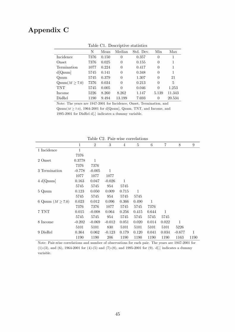
Appendix C

Table C1. Descriptive statisticsN Mean Median Std. Dev. Min Max

Incidence 7376 0.150 0 0.357 0 1Onset 7376 0.025 0 0.155 0 1Termination 1077 0.224 0 0.417 0 1d[Qnum] 5745 0.141 0 0.348 0 1Qnum 5745 0.379 0 1.307 0 21Qnum(M � 7:0) 7376 0.034 0 0.213 0 5TNT 5745 0.005 0 0.046 0 1.253Income 5226 8.260 8.262 1.147 5.139 11.343DisRel 1190 9.494 13.199 7.693 0 20.534Note: The years are 1947-2001 for Incidence, Onset, Termination, and

Qnum(M � 7:0), 1964-2001 for d[Qnum], Qnum, TNT, and Income, and

1995-2001 for DisRel d[.] indicates a dummy variable.

Table C2. Pair-wise correlations1 2 3 4 5 6 7 8 9

1 Incidence 17376

2 Onset 0.3778 17376 7376

3 Termination -0.778 -0.005 11077 1077 1077

4 d[Qnum] 0.163 0.047 -0.026 15745 5745 954 5745

5 Qnum 0.123 0.050 0.009 0.715 15745 5745 954 5745 5745

6 Qnum (M � 7:0) 0.023 0.012 0.096 0.366 0.490 17376 7376 1077 5745 5745 7376

7 TNT 0.015 -0.008 0.064 0.256 0.415 0.644 15745 5745 954 5745 5745 5745 5745

8 Income -0.202 -0.069 -0.012 0.051 0.020 0.014 0.022 15101 5101 830 5101 5101 5101 5101 5226

9 DisRel 0.364 0.062 -0.123 0.179 0.120 0.041 0.034 -0.677 11190 1190 206 1190 1190 1190 1190 1163 1190

Note: Pair-wise correlations and number of observations for each pair. The years are 1947-2001 for

(1)-(3), and (6), 1964-2001 for (4)-(5) and (7)-(8), and 1995-2001 for (9). d[.] indicates a dummy

variable.

45

essays on conflict, institutions, and ethnic diversity …...social capital may have its greatest...

Documents