essays on bargaining and coordination games: the role of social … · 2016-06-29 · also known as...
TRANSCRIPT
Thesis submitted to the University of East Anglia for the Degree of Doctor of Philosophy
Essays on Bargaining and Coordination Games:
The Role of Social Preferences and Focal Points
Andreas Dickert
University of East Anglia
School of Economics
22nd January 2016
”This copy of the thesis has been supplied on condition that anyone who consults it is understood to recognise that its copyrights rests with the author and that use of any information derived therefrom must be in accordance with current UK copyright law. In addition, any quotation or extract must include full attribution.”

ii
Acknowledgements
I would like to thank my supervisory team Dr. Anders Poulsen and Professor Robert
Sugden for their continuous support, advice and encouragement throughout the work
of this thesis. I am particularly grateful to them for giving me the opportunity to
explore bargaining situations, which constitute part of my daily work, from an
economic perspective. I thank Dr. Marco Piovesan and Dr. Ben McQuillin who have
kindly accepted to be discussants of this thesis. Also, the research support of the
university and the CBESS centre is greatly appreciated. Furthermore, I thank my
former co-student Kei for additional support and encouragement. Special thanks go
to my former mentor, the late Professor Earl Thompson for inspiration, intellectual
exchange and the insight that science does not only consist of procedural
conventions. Last but not least, I thank my family. My gratitude goes to my parents
for passing on their curiosity in the field of social sciences and for their
encouragement. Also, I am indebted to my brother Stephan for unconditional and
unlimited support as well as constructive criticism. Finally, I thank my wife Jane and
my two beautiful children for their love, patience and support.
Andreas Dickert
University of East Anglia
January 2016

iii
Abstract
This thesis presents three chapters that investigate the role of social preferences,
focal points and loss aversion in bargaining situations. The first chapter contributes
to existing research by examining the effects of loss aversion on players’ ability to
coordinate their claims in a simultaneous two-player battle of the sexes game. In this
game, two objects worth a different monetary value are placed on a symmetrical
spatial grid, eliciting spatial proximity as a potential payoff-irrelevant focal point. A
failure to claim separate objects leads to a net loss for both players. Results show
that the introduction of potential losses creates a preference to choose the less
profitable option in order to avoid a loss. The second chapter adds to recent research
by investigating how Asian vs. Western cultural backgrounds and corresponding
levels of self-interest influence bargaining results in intercultural bargaining games.
Results show that self-interest is a reliable predictor of offer levels. Further, self-
interest seems to be a more prominent predictor of offer levels in Eastern than in
Western cultures. The third chapter tests the impact of spatial proximity as a
potential focal point on relationship-specific investments and bargaining behaviour.
Players first made investments, followed by claiming bought objects on a spatial
grid. Different configurations of the objects elicited spatial proximity as a potential
focal point. Results revealed that players did not seem to use the focal point in their
choice behaviour. Furthermore, players seemed mostly concerned with the notion of
proportional equity in line with equity theory. In some cases fairness concerns lead
to inefficiencies. The research in this dissertation has provided further evidence on
how (social) preferences can adversely affect efficient solutions. Future bargaining
interactions should incorporate players’ social preferences and need for safety in a
more holistic approach.

iv
Contents Acknowledgements ..................................................................................................... ii Abstract ......................................................................................................................iii Introduction ................................................................................................................ 1 Chapter 1: Losses in Coordination Games with Payoff Asymmetry - a Bargaining Representation ............................................................................................ 14
1. Introduction ................................................................................................................. 14
1.1 Introduction to loss aversion and bargaining ........................................................... 14
1.2 Focality .................................................................................................................... 15
1.3 Loss aversion and loss avoidance ............................................................................ 17
2. Theoretical framework ................................................................................................ 20
2.1 Costs......................................................................................................................... 21
2.2 A more general case of costs ................................................................................... 22
3. Experiment ................................................................................................................. 23
3.1 Experiment design ................................................................................................. 23
3.2 Experiment procedure ........................................................................................... 23
4. Expected findings ........................................................................................................ 27
4.1 General hypotheses .................................................................................................. 27
4.2 Hypotheses regarding choice behaviour when losses are possible .......................... 28
5. Results ......................................................................................................................... 30
5.1 The rule of closeness ................................................................................................ 31
5.1.1 Choice behaviour ............................................................................................ 31
5.1.2 Summary .......................................................................................................... 33
5.2 The effect of asymmetry .......................................................................................... 35
5.2.1 Choice behaviour ............................................................................................. 35
5.2.2 Coordination .................................................................................................... 37
5.2.3 Summary .......................................................................................................... 40
5.3 The framing effect ................................................................................................... 41
5.3.1 Choice behaviour ............................................................................................. 41
5.3.2 Coordination .................................................................................................... 44
5.3.3 Summary .......................................................................................................... 47

v
5.4 The effect of cost c ................................................................................................... 47
5.4.1 Choice behaviour ............................................................................................. 48
5.4.2 Coordination .................................................................................................... 49
5.4.3 Summary .......................................................................................................... 51
6. Conclusion & discussion ............................................................................................. 51
Chapter 2: The Effect of Culture and Self-Interest on Intercultural Bargaining Games .................................................................................................................................. 57
1. Introduction ................................................................................................................. 57
2. Culture ......................................................................................................................... 60
3. Experiment .................................................................................................................. 63
3.1 Recruiting .............................................................................................................. 63
3.2 Experiment design ................................................................................................. 66
3.3 Experiment procedure ........................................................................................... 70
4. Hypotheses .................................................................................................................. 75
5. Results ......................................................................................................................... 76
5.1 SVO-Measure .......................................................................................................... 76
5.2 Cultural and SVO effects in bargaining ................................................................... 78
5.3 Hypotheses based on theoretical predictions ........................................................... 85
5.4 Consistency of choice .............................................................................................. 86
6. Discussion.................................................................................................................... 87
Chapter 3: The Effect of Payoff-Irrelevant Cues and Fairness on the Hold-Up Problem ............................................................................................................................... 92
1. Introduction ................................................................................................................. 92
1.1 The hold-up problem ............................................................................................... 92
1.2 Related research ....................................................................................................... 93
1.2.1 Communication & fairness concerns ............................................................... 93
1.2.2 Private information & fairness concerns ......................................................... 95
1.2.3 Ownership & reciprocity .................................................................................. 96
1.3 Expanding on current research and aim ................................................................... 97
1.3.1 Expanding on ownership .................................................................................. 97
1.3.2 Expanding on communication ...................................................................... 100
1.3.3 Expanding on fairness ................................................................................... 101
2. Model ......................................................................................................................... 102
2.1 Investment .............................................................................................................. 102
2.1 Bargaining .............................................................................................................. 103
vi
2.3 Equilibria & strategies ........................................................................................... 105
2.4 Fairness concerns ................................................................................................... 108
3. Experiment ................................................................................................................ 111
3.1 Experiment design ................................................................................................. 111
3.2 Hypotheses ............................................................................................................. 117
3.3 Experiment procedure ............................................................................................ 120
4. Results ....................................................................................................................... 123
4.1 Investment results .................................................................................................. 123
4.2 Bargaining ............................................................................................................. 127
5. Conclusion & discussion ........................................................................................... 138
5.1 Comparison with the experiment of E&Ja ............................................................. 139
5.2 Investment behaviour ............................................................................................. 139
5.3 Bargaining behaviour ............................................................................................. 140
5.3.1 Fairness considerations .................................................................................. 141
5.4 Conclusion ............................................................................................................. 143
References ............................................................................................................... 145 Appendix ................................................................................................................. 154
1. Appendix Chapter 1 ................................................................................................... 154
2. Appendix Chapter 2 ................................................................................................... 167
3. Appendix Chapter 3 ................................................................................................... 187
vii
List of Tables
2.1 Regression results for offers ....................................................................................... 83
2.2 Ultimatum Game – Average expected payoffs ........................................................... 84
2.3 AO – Average expected payoffs ................................................................................. 85
3.1a Payoffs for player A and player B if P is split evenly ............................................. 106
3.1b AO – Payoffs for player A and player B if the entire sum is split evenly including endowments ............................................................................................................... 106
3.1c Payoffs for player A and player B if the net surplus is split evenly ........................ 107
3.1d Payoffs for player A and player B if P is split proportionally by investment contributions .............................................................................................................. 108
3.2 Game schedule showing the parameters for each game ............................................ 114
3.3 Example of anticipated payoffs if players split the pie evenly ................................. 117
3.4 Investment results ..................................................................................................... 123
3.5 Comparison of individual games regarding investment activity of favoured players and less favoured players: p-values .......................................................................... 127
3.6 Average claims of both players per game ................................................................ 128
3.7 Agreement distribution by game including games in which there was no investment ................................................................................................................................... 129
3.8 Average net earnings and frequency of positive net earnings in games with agreements ................................................................................................................ 137
3.9 Random sequence of games .................................................................................... 187

viii
List of Figures
1.1 Bargaining Table ........................................................................................................ 20
1.2 Coordination game in normal form: 2x2 matrix of the game ..................................... 20
1.3 Coordination game in normal form with costs ........................................................... 21
1.4 Coordination game in normal form with costs and factor Δ ....................................... 22
1.5 Experiment setup, 3x3 design (general) ...................................................................... 24
1.6 Overview of the treatment parameters ........................................................................ 25
1.7 Comparison of average choice behaviour in all three frames – frequency of choosing the Left object ............................................................................................................. 32
1.8 Comparison of choice behaviour in the Gains frame –frequency of choosing the Left object .......................................................................................................................... 33
1.9 Comparison of choice behaviour in the Mixed frame – frequency of choosing the Left object .......................................................................................................................... 34
1.10 Comparison of choice behaviour in the Loss frame – frequency of choosing the Left object .......................................................................................................................... 34
1.11 Choice behaviour: frequency of the Left and the Right players to choose the focal point ............................................................................................................................ 35
1.12 Expected Coordination Rate – Gains Frame ............................................................ 37
1.13 Expected Coordination Rate – Mixed Frame ........................................................... 37
1.14 Expected Coordination Rate – Loss Frame .............................................................. 38
1.15 Expected Coordination Rate (Near & Far Equilibrium) – Gains Frame .................. 39
1.16 Expected Coordination Rate (Near & Far Equilibrium) – Mixed Frame ................. 40
1.17 Expected Coordination Rate (Near & Far Equilibrium) – Loss Frame ................... 40
1.18 Average frequency of Left and Right players choosing the Left object across all frames ......................................................................................................................... 42
1.19 Comparison of choice behaviour in the three frames-Left players choosing Left object .......................................................................................................................... 43
1.20 Comparison of choice behaviour in the three frames –Right players choosing Left object .......................................................................................................................... 43
1.21 Average expected coordination rate across all frames and average expected coordination rate on the Near and Far equilibria across all frames ............................ 45
1.22 Expected coordination rates across all frames; Expected coordination rates on the Near and Far equilibria ............................................................................................... 50
1.23 Expected coordination rates across all frames for the individual games ................. 50
2.1 Culture Cycle according to Hofstede (2001) .............................................................. 61
2.2 Ring measure .............................................................................................................. 68
2.3 Distributional Games .................................................................................................. 70

ix
2.4 Relative frequencies of SVO-score distribution ......................................................... 77
2.5 Ultimatum Game – Offer Level Frequency Distribution ........................................... 79
2.6a AO1 – Offer levels .................................................................................................... 80
2.6b AO2 – Offer levels .................................................................................................... 80
2.7a Ultimatum Game – Offer Level Frequency Distribution Total In-group vs. Mixed Group .......................................................................................................................... 81
2.7b Ultimatum Game – Offer level Frequency Distribution Eastern In-group vs. Mixed Group comparison ...................................................................................................... 81
2.7c Ultimatum Game – Offer level Frequency Distribution Western In-group vs. Mixed Group comparison ...................................................................................................... 82
2.8 Ultimatum Game – Acceptance levels ....................................................................... 86
3.1 Representation of a spatial grid – the “bargaining table” .......................................... 111
3.2 Representation of the horizontal alignment .............................................................. 112
3.3 Representation of the vertical alignment .................................................................. 113
3.4 Detailed investment distribution of the favoured player .......................................... 126
3.5a Split of net surplus – Game 1 ................................................................................... 131
3.5b Split of net surplus – Game 7 ................................................................................... 131
3.5c Split of net surplus – Game 2 ................................................................................... 131
3.5d Split of net surplus – Game 8 ................................................................................... 131
3.5e Split of net surplus – Game 3 ................................................................................... 131
3.5f Split of net surplus – Game 9.................................................................................... 131
3.5g Split of net surplus – Game 4 ................................................................................... 132
3.5h Split of net surplus – Game 10 ................................................................................. 132
3.5i Split of net surplus – Game 5 .................................................................................... 132
3.5j Split of net surplus – Game 11 .................................................................................. 132
3.5k Split of net surplus – Game 6 ................................................................................... 132
3.5l Split of net surplus – Game 12 .................................................................................. 132
3.6 Favoured player claims versus contribution ............................................................. 134
3.7 Less favoured player claims versus contribution ...................................................... 134

1
Introduction
Searching for an agreement regarding the exchange or division of a good,
also known as bargaining, is one of the “most basic activities in economic life”
(Camerer, 2003). In order to reach agreement, often people have to make best-guess
assumptions about other people’s preferences and valuations of goods (forming
beliefs) as no other information is available. The uncertainty about the other party’s
future actions in a bargaining situation often prevents people from choosing optimal
strategies to reach desired outcomes. However, the individual valuations of a good
are private until shared in some form of interaction including bargaining. Valuations
are determined by people’s circumstances, beliefs and preferences as well as “human
interaction in the context of scarcity”, a central theme to Economics (Heyne et al.,
2006).
The exchange of information can be direct via communication and indirect
via showing one’s preferences through behaviour. Bargaining serves as an example
of an indirect way to determine people’s individual preferences. In some cases a
bargaining interaction can have a cooperative setting in which people work together
in order to maximize a mutual gain, and in other cases it can have a competitive
setting, in which people try to maximize their own gain at the expense of another
person. Cooperative and competitive approaches to bargaining often depend on how
scarce a resource is as well as on agents’ intentions. Some bargaining scenarios
require both cooperative and competitive behaviour, but at different stages. In any
bargaining situation the information available regarding people’s preferences and
valuations of goods often decides about making a profit or making a loss or whether
a good can be split efficiently.
People attempt to compensate for their lack of information by utilizing any
observed information, stereotypes, situational cues or past experiences to infer about
another person’s possible course of action. Characteristics of the other person, such
as ethnicity, gender and social group or past observed behaviour let people infer
about general behaviour. In particular, preferences emerging in connection with the
society we live in – social preferences (e.g., a preference for treating each other
fairly, altruistic behaviour, self-interest, reciprocating another person’s behaviour,
aversion against unnecessary inequality) – have inspired a vast body of research in

2
economics. Still, many questions are unanswered regarding how people formulate
optimal strategies. Among a plethora of unanswered questions, a currently relevant
question in research is whether and how players can utilize payoff-irrelevant
information to find optimal strategies when facing potential losses. It is also unclear
whether post-investment exploitation can be remedied by payoff-irrelevant focal
points. Additionally, the question remains whether optimal strategies are subject to a
particular preferable set of culturally determined preferences.
Contributing to existing research, this dissertation investigates two-sided
bargaining situations in which economic agents, henceforth players, are faced with
the task of finding optimal, payoff-maximizing strategies congruent with their own
social preferences and their best guess about the other player’s behaviour. The
experiments in this dissertation investigate three key scenarios in which players have
to align their preferences and beliefs in order to achieve a successful outcome. In the
first experiment, players are expected to make strategy choices in terms of
coordinating the split of a sum while facing a potential loss in case of coordination
failure. In the second experiment, players are expected to split a monetary amount in
intercultural and intracultural settings. In the third experiment, players are asked to
coordinate their strategies in a two stage hold-up scenario (including investment in
the first stage), when being presented with additional payoff-irrelevant information.
Next I present the concepts, research questions, as well as definitions and necessary
backgrounds for the experiments.
Bargaining, coordination and social preferences
The key research questions, key concepts to investigate bargaining behaviour
in the different chapters, as well as key results are briefly summarized and defined
below. Chapter 1 focuses on the concepts of loss aversion, focal points and
coordination. Chapter 2 focuses on the concept of culture and cultural dimensions, as
well as self-interest in the context of bargaining (ultimatum games and alternating
offer bargaining games). Finally, Chapter 3 deals with hold-up scenarios, fairness
concerns as well as focal points.
3
Chapter 1
In Chapter 1, I investigate bargaining and coordination behaviour with
potential losses. Players are asked to split an amount of money by simultaneously
claiming one of two particular objects worth a certain monetary value. Players are
not able to communicate with each other and in case they accidentally claim the
same object, the objects remain on the table and both players incur a loss.
Coordinating claims without possible communication are risky, as both players have
a 50% chance to get it right. In order to facilitate coordination for the two players,
strategy labels are introduced as payoff-irrelevant information to serve as potential
focal points. Previous research has focused on coordination problems involving focal
points under payoff symmetry (Schelling, 1960; Mehta et al., 1994a,b) and payoff
asymmetry (Crawford et al., 2008; Isoni et al., 2013, 2104). General results from this
research suggest that payoff-irrelevant information serves as a label-salient focal
point in situations in which the payoff for both players is the same. If payoffs
become asymmetric, payoff-irrelevant information becomes less important. Adding
to existing research, I investigate whether payoff-irrelevant information becomes a
salient decision criterion when players are punished for not coordinating by incurring
losses.
Coordination tasks including losses can easily be extended to the real world.
A good example is Wal Mart and its successful and rapid growth in the United States
since 1962. As described in Walton (1992), Wal Mart’s successful expansionary
strategy was based on the strategic placement of distribution centres. In rural areas
more than one distribution centre could not be sustained if markets had to compete
for customers, which would lead to a price war and subsequent losses. As a result,
the retail chains had to “coordinate” placing their stores and distribution centres.
Experiment, concepts and results
In order to investigate the choice behaviour of players, I designed a
laboratory experiment in which subjects were asked to select one out of two objects
worth a certain monetary value presented to them in a symmetric spatial grid,
henceforth bargaining table. The objects were located in close proximity to
rectangles representing the two players on that spatial grid. The spatial proximity of

4
the objects to the players’ bases served as payoff-irrelevant focal point. The “rule of
closeness” (Mehta et al., 1994a,b) suggests players coordinate by picking the object
nearest to their base. In my experiment picking the same object is considered a
coordination failure and players are punished by losing money from their
endowment. In different scenarios the monetary value of the two objects as well as
the possible loss for coordination failure was varied, allowing me to investigate
people’s choice behaviour associated with these different payoffs.
In order to understand the effect that potential losses have on people’s
behaviour, some concepts of loss aversion and loss avoidance are critical. Loss
aversion, as employed in prospect theory (Kahneman & Tversky,1979) is the notion
that “losses loom larger than gains”. This very basic notion describes the finding that
the pain of losing a specific amount weighs more than the pleasure of gaining the
same amount. For example, a person that loses 1£ experiences a dissatisfaction that
is larger than the satisfaction would be of receiving 1£. Loss aversion is relative,
meaning that losses as well as gains are always perceived in relation to a reference
point. In the simple example above, the reference point would be 0£. Kahneman and
Tversky (1979) explain this phenomenon with an “s-shaped” function, which is
concave for gains and convex for losses.
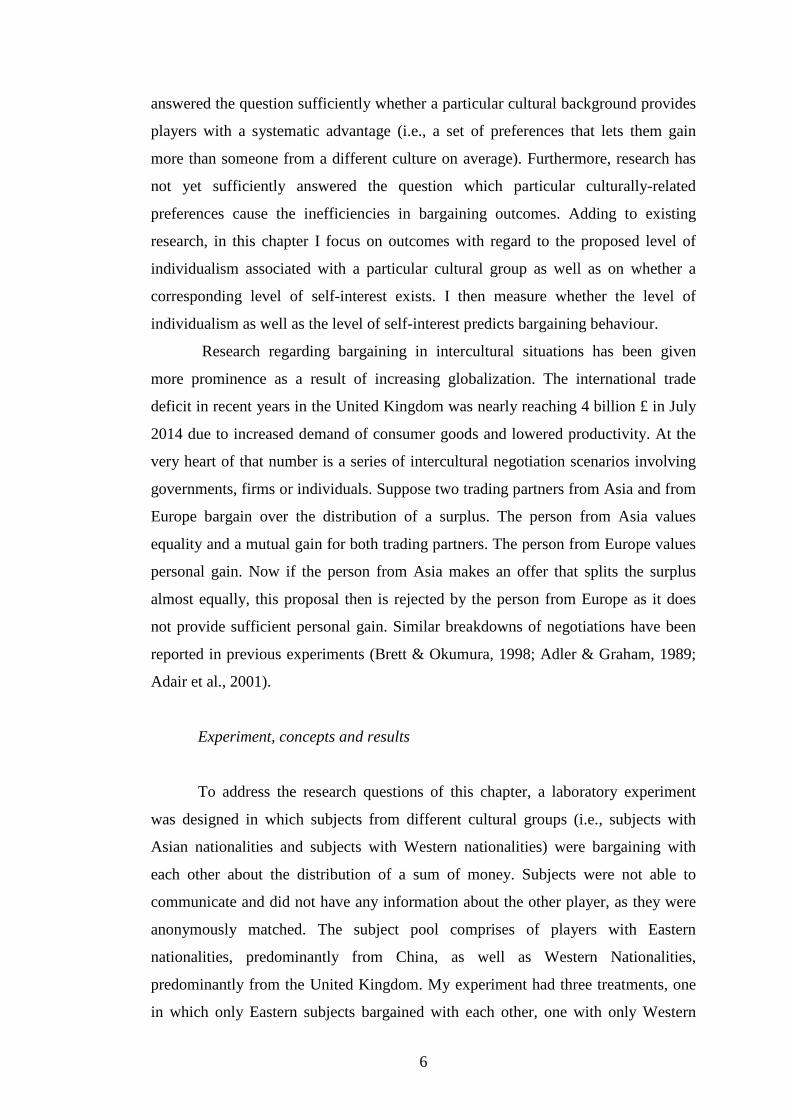
Example of an S-shaped utility curve in a typical Cartesian coordinate system showing players value
v(x) in relation to an outcome x - (Kahneman and Tversky, 1979).
In the above figure, x depicts the outcome and V(x) depicts the subjective
value associated with the outcome. Preferences change as the outcome becomes

5
negative. Interestingly, little evidence of loss aversion in coordination scenarios
exists. Research investigating losses interactive bargaining situations showed that
players avoid strategies leading to a sure loss In favour of strategies leading to a
possible gain, one aspect of loss avoidance theory (Feltovich et al., 2012). The
prediction in my experiment was that according to Nash equilibrium theory losses
improve coordination. Focal point theory suggested that players utilize the rule of
closeness and coordinate better than randomizing their choices with ½. Due to
looming losses, players have stronger incentive to coordinate and use the “rule of
closeness”.
The most relevant finding of this experiment is that potential losses do not
improve coordination rates. Players show signs of loss aversion and make their
choices according to payoff relevant cues. In case of payoff asymmetry, players both
tend to choose the low payoff, leading to coordination failure. Subjects show a
willingness to allocate the higher payoff to the other player as they perceive this as
the safer strategy. This result implies a similar payoff bias found in experiments
regarding coordination under payoff asymmetry by Crawford et al. (2008). Players
assume that the other player would choose the high payoff and choose the low
payoff. Focal points lose prominence if they are in contrast to more salient efficiency
criteria, such as payoffs and losses.
Chapter 2
The next chapter investigates whether cultural background (i.e., nationality)
as well as the degree of self-interest has an impact on offer and acceptance levels in
bargaining scenarios in which two players divide up a pie. The basic idea is that
players from a certain nationality behave in a particular way in bargaining situations
in terms of making offers and also accepting offers. Often it is found that the
different bargaining behaviour based on culturally based preferences leads to
inefficiencies (i.e., suboptimal bargaining outcomes). To this date, research found
overwhelming evidence that players are sensitive to who they bargain with,
particularly sensitive to cues based on cultural background (Ferraro & Cummings,
2007; Brett & Okumura, 1998). Experimental results have shown that players in
intercultural bargaining situations often realize less profit than they would have in
intracultural bargaining situations (Brett & Okumura, 1998). So far, research has not
6
answered the question sufficiently whether a particular cultural background provides
players with a systematic advantage (i.e., a set of preferences that lets them gain
more than someone from a different culture on average). Furthermore, research has
not yet sufficiently answered the question which particular culturally-related
preferences cause the inefficiencies in bargaining outcomes. Adding to existing
research, in this chapter I focus on outcomes with regard to the proposed level of
individualism associated with a particular cultural group as well as on whether a
corresponding level of self-interest exists. I then measure whether the level of
individualism as well as the level of self-interest predicts bargaining behaviour.
Research regarding bargaining in intercultural situations has been given
more prominence as a result of increasing globalization. The international trade
deficit in recent years in the United Kingdom was nearly reaching 4 billion £ in July
2014 due to increased demand of consumer goods and lowered productivity. At the
very heart of that number is a series of intercultural negotiation scenarios involving
governments, firms or individuals. Suppose two trading partners from Asia and from
Europe bargain over the distribution of a surplus. The person from Asia values
equality and a mutual gain for both trading partners. The person from Europe values
personal gain. Now if the person from Asia makes an offer that splits the surplus
almost equally, this proposal then is rejected by the person from Europe as it does
not provide sufficient personal gain. Similar breakdowns of negotiations have been
reported in previous experiments (Brett & Okumura, 1998; Adler & Graham, 1989;
Adair et al., 2001).
Experiment, concepts and results
To address the research questions of this chapter, a laboratory experiment
was designed in which subjects from different cultural groups (i.e., subjects with
Asian nationalities and subjects with Western nationalities) were bargaining with
each other about the distribution of a sum of money. Subjects were not able to
communicate and did not have any information about the other player, as they were
anonymously matched. The subject pool comprises of players with Eastern
nationalities, predominantly from China, as well as Western Nationalities,
predominantly from the United Kingdom. My experiment had three treatments, one
in which only Eastern subjects bargained with each other, one with only Western

7
subjects and one with mixed subjects. In my experiment I used simple alternating
offer and ultimatum games. In each of the treatment subjects were not informed
which nationality the bargaining partner had. Offer levels and acceptance rates as
well as agreement levels were measured. Also, prior to the experiment players had to
complete 24 distributional tasks in which they were asked to decide between two sets
of payoffs for themselves and the co-participant. These distributional games were
used in order to determine players’ level of self-interest by measuring their Social
Value Orientation (SVO-Score).
Social Value Orientation measures preferences of people regarding the
distribution of resources. According to the theory based on Griesinger & Livingston
(1973) and Van Lange (1999) people can be pro-self (i.e., like for them favourable
outcomes) or pro-social (i.e., like favourable for the next person) to different
degrees. The choice behaviour in the distributional games is measured and
transferred to a score. The score can be grouped into certain categories. People who
are grouped as individualists mainly are concerned with their own benefit without
regarding the other person’s outcome. Competitive players maximize their own
outcome and minimize the outcome of the other person. Cooperative players
maximize their own outcome and the outcome of the other player. Lastly, altruists
are only concerned with the outcome for the other player. Overall the SVO-measure,
next to surveys seemed to be the most logical way to determine players’ orientation.
One interesting question is what exactly constitutes “culture”. While there are
several scientific explanations for this term, in this experiment I focus on the level of
individualism as one attribute in the model of Hofstede (2001) describing the level of
interdependence of people in a particular group. Other attributes in this model that
were not considered are power distance (i.e., degree of preference for achievements),
masculinity (i.e., degree of preference for achievements), uncertainty avoidance (i.e.,
anxiety regarding the unknown) and long term orientation (i.e., future oriented
perspective). Out of these “cultural dimensions” individualism has been researched
most and was attributed as a possible cause for the breakdown of bilateral bargaining
agreements (Brett & Okumura, 1998). According to Hofstede (2001), people in
Asian nations and people in Western nations show a significant difference in terms
of individualism. Of course individualism should not be confused with self-interest.
Someone that is individualistic is oriented mostly to himself in terms of his thinking
and actions, but can still be an altruistic person.

8
The main findings in my experiment are showing that the level of self-
interest predicts offer levels in both cultures. Further, the level of self-interest is not
predicted by a particular level of individualism as defined by Hofstede (2001). Also
offer levels were not predicted by nationality (cultural background). However, some
cultural effects were found. Self-interest predicts offer levels better for Eastern
subjects than for Western subjects. Hence, Eastern subjects are more sensitive to
self-interest levels. Some signs of discrimination were observed, such as players
making higher offer levels in the mixed frame. Overall the study did not find that
players with a particular cultural background have a systematic advantage in
bargaining as a result of their culturally based preferences.
Chapter 3
The last chapter of this dissertation investigates the influence of spatial
proximity on players’ investment and bargaining behaviour in a hold-up scenario.
Prior to a two-player bargaining situation, players simultaneously decide how much
of their endowment they will invest. In principle, once the investment is made, costs
are sunk, and players do not have a guarantee that they recover any investment made
in the following bargaining stage. As a result, it is often observed that there is no
investment, as the investor does not want to be exploited. Often players cannot
communicate prior to investing and do not have any knowledge regarding the other
player’s choices. Past research focused on mitigating underinvestment and found that
direct, pre-investment communication remedies the problem partially (Ellingsen &
Johannesson, 2004a,b), as well as pre-investment allocation of ownership rights
(Fehr et al., 2008). However, underinvestment could not be mitigated fully and some
room for coordination failure in the bargaining stage remains. A partial reason for
coordination failure is the type of bargaining situation presented to players in past
research. Players often were confronted with simultaneous, one-round games, in
which a failed coordination of claims and demands leads to a payoff of zero. Also, if
players made agreements regarding any split before investing, they did not act as it
was agreed. Past experiments almost unanimously found that choice behaviour could
be explained by different degrees of fairness concerns (e.g., Ellingsen &
Johannesson, 2004a,b). So far, research has not yet solved the problem of
underinvestment and coordination failure entirely. While there are some approaches

9
that somewhat mitigate the underinvestment problem with direct communication,
little research has been conducted regarding the effect of spatial proximity (as
defined in Chapter 1) on players’ choice behaviour in the bargaining and the
investment stage. While it has been shown that pre-investment determination of
ownership rights has a positive effect on remedying underinvestment, it has not been
determined whether players are able to use spatial proximity as a focal point in order
to coordinate their strategies. The question is that if investment profits were
displayed on a bargaining table while clearly displaying the contribution of each
player, whether players would use these spatial cues in order to divide the surplus
from investment. If players as a result anticipated a fair split, they would invest.
Further, it is unclear how players’ exhibit fairness concerns exactly. Adding to
existing research I introduce focal points in terms of spatial proximity to the hold-up
problem, and I shed further light on the influence of fairness on players’ choice
behaviour by comparing two different fairness concepts.
Experiment, concepts and results
I experimentally tested whether players substitute ownership with spatial
proximity and are able to coordinate their investment and bargaining behaviour. In
each experiment players were anonymously paired up and presented with the task to
make an investment, followed by a bargaining stage in order to divide the surplus.
Half of the players in each session received a small or no endowment and half of the
players received a larger endowment. In each two-player bargaining situation, a
player with a low endowment was paired with a player with a large endowment.
Players were unable to communicate prior to or during the game. They could make
an investment by purchasing several circular objects worth a certain monetary value.
After investment, the objects were placed on a bargaining table. In order to
investigate the effect of spatial proximity in some games objects were placed
vertically on the bargaining table at equidistance to the two players bases and in
other games the objects were placed next to the base of the player that purchased
them. Players then were engaging in a free-form bargaining game lasting 90 seconds
in order to reach an agreement. An agreement is reached if both players agree on an
allocation of the objects and the total number of objects claimed is equal or smaller
than the number of objects on the bargaining table. If no agreement is reached, both
10
players receive a payoff of zero. In theory players should split the objects as
suggested by spatial proximity. As fairness concerns were a predominant decision
rule in past research, particular emphasis was laid on inferring players fairness
concerns as suggested by their choice behaviour.
I investigate two main concepts of fairness. Fairness concerns in terms of
inequity aversion as defined by Fehr & Schmidt (1999) suggest that players incur a
loss of utility if their payoff is either higher (superiority aversion) or lower
(inferiority aversion) in comparison with the other player. Depending on players’
preferences, the highest utility is reached if both players gain the same amount of net
surplus from the pie. According to the model of Fehr & Schmidt, different clusters of
population exist, each willing to accept a different share of the pie. In my experiment
inequity aversion was measured by investigating to which degree the player with the
lower starting endowment was compensated for this asymmetry by the player with
the larger endowment. Also, it was investigated whether players looked for equal
splits of the surplus and to which degree players looked for equal splits of the total
amount in the game. A further concept introduced into that game is proportion as
defined by equity theory (Adams, 1965). Equity theory would assume that players
find a division of the pie that reflects the level of their contribution to the overall
amount to be split. Players then would find it fair if both players receive exactly the
same ratio out of investment and share of the pie.
The main findings of my experiment can be summarized as follows. Players
did not incorporate spatial proximity into their decision making process. However,
results show that players were concerned with proportionality when dividing up the
pie. In addition, some signs of inequity aversion could be observed as players did
compensate for lower initial endowment levels in their decisions. It was further
found that players with a higher endowment invested predominantly on the level of
the maximum endowment of the player with the lower endowment. This is
considered as a “safe” strategy next to not investing at all. Players then often
proceeded to split the pie equally. In this case both players did forgo higher payoffs
in order to equate their risk to be exploited. In this case, fairness concerns cause
inefficiencies. In summary, spatial proximity does not seem to mitigate
underinvestment fully. However, players in my design invested more than in
comparable games in the experiments of Ellingsen & Johannesson, (2004a). A visual
representation of payoffs can aid players to some extent, and players are more

11
confident about not being exploited as a result of the possibility of cheap talk in the
bargaining session. Players were most concerned on how to reach a proportional
outcome and to minimize the risk of exploitation.
Conclusion
The experimental results in this dissertation provide further insight into
players’ choice behaviour in bargaining situations, reflecting their personal
preferences regarding losses, self-interest and culture and fairness. In addition, the
salience of payoff-irrelevant cues is investigated. Looking at bargaining interactions
from three different angles helped to elucidate people’s motivations when interacting
in bargaining.
The fact that people tend to sacrifice gains in order to avoid losses in
coordination games does have some implications real world problems. In the
example of Wal Mart opening superstores in remote locations that can only sustain
one particular superstore, the strategy would have been clear. In case of possible
conflict, ceteris paribus, Wal Mart would pay less attention to the store being in close
proximity to its distribution centres and would focus on finding a location that is
somewhat less attractive in comparison with others. In that way, losses could
potentially be minimized. This of course excludes all other factors necessary for a
decision, such as price competition policy, predatory competition policies, price
changes in transportation costs and other strategic considerations. Wal Marts strategy
focused on being in a particular location first, and then attempting to prevent entry.
Nevertheless, the general application of the finding is relevant and highlights
people’s strategies of loss prevention. Further research could elucidate this finding
by extending the strategy choices of players with regard to incurring higher losses.
Since players are affected in their decision making process by the height of the
possible loss, it can be conjectured that, as losses increase, players will at some point
switch their decision making to include spatial proximity. Also it could be the case
that the salience of a payoff-irrelevant focal point needs to be established as a
convention in the market first.
Furthermore, this dissertation gives support for the notion that players are
influenced in their decision making by self-interest and indirectly by culture. While
offer levels and self-interest levels were not predicted by cultural background, some

12
culturally related effects could be found. While cultural background does not predict
self-interest, for Eastern subjects offer levels are predicted better by their social
preferences. Belonging to a certain cultural group did not provide players with a
systematic bargaining advantage.
Applied to the real world, this result suggests that when players from
different cultures interact in a bargaining scenario, it would be wise to know the
individual level of self-interest of this person. Also, when bargaining with someone
from an Eastern culture it is good to know that self-interest levels matter more than
when bargaining with someone from Western cultures. Future studies should
incorporate more cultural variables next to individualism. Also, further studies
should select subjects from different countries that do not have any other affiliation
to any particular group.
Lastly, players are sensitive to the possibility of exploitation as theory
predicts. However, in contrast to theoretical predictions, players seek to mitigate that
risk by reciprocating the level of investment of the player with the lower endowment.
In order to achieve that, they forgo larger gains. In that regard, fairness concerns are
the cause of underinvestment. Also, it appears that people are concerned with
relational equity meaning a proportional distribution with regards to their own level
of contribution. As spatial proximity is not a sufficiently salient focal point, players
cannot use the suggested distribution by the focal point to achieve higher investment
rates.
I conjecture that underinvestment in a hold-up situation is sensitive to the
form of bargaining as well as the presentation of the surplus. Indirectly this would
mean that payoff-irrelevant information does to some degree influence players. Also,
the possibility of a risk equilibrium might be essential. While players are concerned
with relational equity, they do prefer to play it safe. However, the higher investment
rates (when compared with Ellingsen & Johannesson, 2004a,b, under the no-
communication premise) suggest that future research should put more emphasis on
factors such as risk involved and presentation of the bargaining scenario.
In conclusion, I find that players are seeking a safe strategy that minimizes
risk whenever possible. Players are concerned with payoff, degree of self-interest as
well as proportional equity. The reason that payoff-irrelevant cues are not so
prominent could be caused by the growing money bias in modern society.
Culturally-related behaviour is also influenced by values that are reinforced by the

13
war for resources and wealth, where globalization makes value systems continuously
more homogenous. The research in this dissertation has provided further evidence on
how (social) preferences can adversely affect efficient solutions. Future bargaining
interactions should incorporate players’ social preferences and need for safety in a
more holistic approach.

14
Chapter 1 Losses in Coordination Games with Payoff Asymmetry - a Bargaining Representation
1. Introduction
1.1 Introduction to loss aversion and bargaining
Successful coordination in a simultaneous move game, without cues
regarding other people’s courses of action and the possibility of communication, is
often difficult to achieve. A known example of this is the battle of the sexes game.
This describes a coordination problem for two decision makers who “win” if they
manage to make a choice that matches the choice of the other person, and who
receive considerably less if they fail to do so. The absence of any information forces
people to make best guesses based on beliefs about the other person’s course of
action. In this situation, non-payoff-related strategy labels (i.e. focal points) could
provide helpful cues for the decision-makers. Researchers have investigated the
effects of non-payoff-related cues as potential focal points in an attempt to improve
coordination (e.g., Schelling, 1960; Mehta et al. 1994a,b; Bacharach, 1997). Other
information (such as possible payoffs) could be influencing a decision-maker’s
choice in a coordination scenario, besides the non-payoff-related strategy labels
(such as focal points). Indeed, recent research has shown that the level of available
profits in such a strategic interaction can influence the decision-maker’s choice,
especially if payoffs are asymmetric (Crawford et al. 2008). In such a scenario,
payoff-irrelevant focal points lose their influence on decision-makers. However it is
unclear, whether this generalises to scenarios in which payoffs can be negative and
whether coordination failure would result in losses.
Contributing to existing research, this chapter explores the effects of different
asymmetric payoff-levels and potential losses upon a decision-maker’s choice in
coordination games. In particular, I examined the effects of losses upon interactions
between two decision-makers in coordination games. For my research the concepts
of loss aversion (Kahneman & Tversky, 1979; Kahneman, Knetsch & Thaler, 1990)
as well as loss avoidance (Feltovich et al., 2012) were of particular importance. In

15
my study I used a spatial grid as a visual representation of a simple battle of the
sexes game as shown in Figure 1.1, which makes strategy choices more obvious and
more natural to the decision-maker. The bargaining table in Figure 1.1 represents an
extension of the experiments conducted by Mehta et al. (1994a) (experiments 11 –
16). An important feature of the bargaining table is the complete spatial symmetry in
which two rectangular bases are placed on the right and on the left of the grid; each
representing one of the players. The amount to be bargained over is then placed in
the form of several circular objects (henceforth objects) in a particular spatial
configuration on the spatial grid. The objects have different spatial proximities to the
two rectangular bases. This design was chosen as players, ceteris paribus, naturally
apply the “rule of closeness” in order to claim objects. The “rule of
closeness“ (Mehta et al., 1994a,b) describes the tendency of players to choose the
object nearer to them when having the choice between two identical objects located
at an unequal distance to them. In this type of design, spatial proximity acts as a non-
payoff-related, label salient focal point. For example, using the “rule of closeness”,
players managed to achieve high coordination rates in payoff-symmetric games
when instructed to coordinate (Mehta et al., 1994a,b). The application of asymmetric
payoffs with the possibility of losses adds a new dimension to this type of
coordination task.
The remaining chapter is structured as follows: after providing a basic
overview of loss aversion in bargaining experiments in the remainder of Section 1,
the theoretical framework of the model is introduced in Section 2. Sections 3 and 4
describe the experiment design and expected results. Section 5 presents the results of
the experiment. Then, Section 6 concludes with a discussion of the results and
implications for further research.
1.2 Focality
Contrary to traditional game theory, the early work of Schelling (1960) found
that the salience of decision labels provides players with cues to successfully
synchronise their behaviour. Schelling (1960) asked people to meet in New York
City without previous communication. If two people were to coordinate by choosing
the same location out of many possible locations, they would receive a reward.
However, if they did not manage to coordinate, they would get a payoff of zero. In

16
this very rudimentary setup, Schelling (1960) found high expected coordination rates
and demonstrated for the first time that a decision label could be a “focal point”, in
this case the Grand Central Station. In another version of this game investigated by
Schelling (1960), subjects were obliged to coordinate on calling either heads or tails
of a coin. This experiment was formally repeated by Mehta et al. (1994a) in which
they obtained similar outcomes. Schelling’s (1960) informal experiments found
above-average coordination rates on “heads”, which he explained with the existence
of a “focal point”. Players predominantly focused on this decision label, as they
clearly preferred “heads” rather than “tails”.
The existence of focal points has been more formally investigated and
documented in recent literature, which found that label-salient focal points are
influenced by payoff-symmetry (Mehta, Starmer and Sugden, 1994a,b; Crawford et
al., 2008; Bardsley et al., 2010; Isoni et al., 2013, 2014). In most of the conducted
experiments, payoffs were symmetrical for participating players. Initially, it was
assumed that the power of a focal point was sufficiently strong even if payoffs were
not symmetrical (Sugden 1995, pg. 548). This assumption has been further
investigated by Crawford et al. (2008), who contend that “when payoffs are even
minutely asymmetric and the salience of labels conflicts with the salience of payoff
differences, salient labels may lose much of their effectiveness and coordination
rates may be very low” (p. 1456). Crawford et al. (2008) further found that
coordination failure is connected to the asymmetry of payoffs.1 One key experiment
of Crawford et al. (2008) was the X-Y game, in which players chose simultaneously
either the labels X or Y. If both players chose the same strategy, they successfully
coordinated and received the designated payoff. In case of failure to coordinate, none
of the two players would receive a payoff. With small payoff-differences, players
chose in favour of the other participants’ payoff (i.e. allocating the higher payoff to
the other player). According to Level-K theory, as payoff differences increase,
players attempt to maximize their own payoff. The results of Crawford et al. (2008)
suggest a strong payoff-bias in players’ decision-making in case of payoff-
asymmetry, where players utilise label salient focal points much less.
1 The work of Crawford et al. (2008) uses a Level-K model to explain why with increasing payoff-asymmetry, players became more payoff-biased in their choices, increasingly favouring their own payoffs, and disregarding the label salient strategy choice for coordination.

17
While according to Crawford et al. (2008) Level-K theory explains the
pattern of coordination failure as payoff-differences increase, Nash equilibrium
theory suggests that overall coordination decreases with increasing payoff-
asymmetry (Appendix 1.1). Research in this field so far has omitted to include the
effect of losses in such a coordination scenario. While Nash equilibrium theory
suggests an improved coordination when losses are introduced, the question is
whether the salience of a strategy label increases if players are punished for
coordination failure by incurring losses. Particularly, the underlying psychological
aspects of loss aversion (prospect theory) and loss avoidance are crucial to
understanding players’ choice behaviour when losses loom.
1.3 Loss aversion and loss avoidance
Choice behaviour in interactive bargaining situations with potential losses has
been mainly explained by the concepts of loss aversion and loss avoidance. Loss
aversion as part of prospect theory and subsequent research, (i.e. first to third
generation prospect theory as in Kahneman & Tversky, 1979; Kahneman, Knetsch &
Thaler, 1990; Luce & Fishburn, 1991; Tversky & Kahneman,1991, 1992; Schmidt et
al., 2008; Erev et al., 2008) is based on the principle that the disutility of a loss
outweighs the utility of an equivalent gain. In fact, “losses loom larger than gains”,
which is captured in an S-shaped value curve in prospect theory (Kahneman and
Tversky, 1979, 1992). This S-shaped value curve possesses the property that it is
steeper in the loss domain, having a convex shape and flatter in the gains domain,
having a concave shape. According to prospect theory, this generally results in
people’s risk aversion in the gains domain and risk seeking behaviour in the loss
domain. In the underlying expected payoff-function, decision weights are applied for
the probabilities of obtaining a payoff as well as the payoff itself. A general
phenomenon is that decision weights are applied so that small probabilities are over-
weighed and larger possibilities are under-weighed, leading to the condition that
decision weights applied are non-linear. These important observations were extended
by a second generation prospect theory model for choice situations with unknown
probabilities (Kahneman & Tversky, 1992). In a typical experiment, a larger number
of decision-makers would take a certain outcome over the chance of receiving a
higher outcome with 80% and receiving nothing with 20%. However, when faced

18
with losses, decision-makers would choose the gamble over the certain loss. Some
important underlying axioms of this theory are transitivity, dominance and
invariance. Further, Tversky and Kahneman (1986) showed that the framing of the
loss may result in a change of preferences of the decision-maker. This argument
stems from the fact that losses (as well as gains) are always measured in relation to a
reference point.
Loss aversion can be found also in strategic interactions, however it is more
difficult to measure. While the effect of loss aversion has been thoroughly
investigated (e.g., in Kahneman, Slovic, & Tversky, 1982), loss aversion in an
interactive environment, such as in a bargaining situation, has not yet been explored
to a greater extent. Kahneman, Knetsch and Thaler (1990) contend that concession
aversion defines the actions of the decision-makers in a bargaining environment.
Concessions made to the other decision-maker are treated as losses, while
compensation received are treated as gains. In accordance with loss aversion,
decision-makers overvalue what they give compared with what they get. Of
particular importance for both players is their status quo, the starting point of the
bargain. Such bargaining and cooperation scenarios are investigated with respect to
international politics in Jervis (1978), Keohane (1984), Grieco (1990), Stein and
Pauly (1992) and Richardson (1992). A similar concept to concession aversion is the
status quo bias (Samuelson & Zechhauser, 1988; Levy 1996), which states that
agents are willing to undergo some effort to protect the status quo if they believe a
change to be leading to potential losses. Concession aversion as well as the status
quo bias, are driven by players overvaluing losses, consistent with loss aversion.
Players would only incur a risk making a change from the status quo is not
acceptable to them.
Generally, only some research is available that investigates losses in a
bargaining context, however, findings in the literature suggest that loss aversion in a
bargaining prove to be disadvantageous for the more loss-averse player (Shalev,
2000). Additionally gender effects under this situation have been found (Schade et
al., 2010), where female subjects use mixed strategies twice as often as male subjects,
leading to potential coordination failure. Additionally, bargaining failure can be an
equilibrium outcome when losses are present (Butler, 2007).
Further, a related concept to loss aversion is loss avoidance, which is defined
as the tendency to avoid choices that yield negative payoffs with certainty in favour
19
of choices that have a possibility of a positive outcome (Cachon and Camerer, 1996).
The notion of loss avoidance has been tested by Rydval and Ortmann (2005), and
Feltovich et al. (2012) using Stag-Hunt games (Rousseau, 1973) to test equilibrium
selection with varying payoff-levels. Although strict loss frames are not tested, the
experiments of Rydval and Ortmann (2005), as well as Feltovich et al. (2012) show
that changes in payoff-levels have an effect on the equilibrium outcome. In another
experiment, Feltovich (2011) investigates the effect of losses in a set of Hawk-Dove
games (with high and low payoffs) and Stag-Hunt games. The low set of payoffs
leads to a negative payoff for both players if the Hawk-strategy was mutually chosen.
The games are strategically equivalent although payoffs vary. Feltovich (2011) puts
forward the hypothesis that the Dove-strategy is chosen more often when losses are
present. In both fixed and random matching, players did choose the Dove-strategy
significantly more often in the low payoff game. The Dove-strategy represents the
“safe” strategy for a player as he is content to get a lower payoff, rather than risking
a negative payoff.
In particular, loss avoidance in a strategic interaction could be observed in the
experiments of Feltovich et al. (2012). In the experiment, subjects are confronted
with three different Stag-Hunt games with high, medium and low payoff-levels. The
medium and low payoff-levels were designed to include potential and certain losses.
During the experiment, the number of times the games were played, the matching
procedure (random versus fixed matching), as well as the level of payoff information
were varied. Players encountered each game only once including (1) full payoff-
information, (2) one without full payoff-information, (3) a treatment in which
players repeated each game with randomly matched players, also under full payoff-
information and (4) one without full information. Results imply that over all
treatments differences in choice behaviour were present due to loss avoidance.
Similarly to the latest experiments of Feltovich (2011) and Feltovich et al. (2012),
players were requested in my experiment to choose between a high and a low payoff,
facing potential losses. The above concepts are considered starting points to predict
players’ behaviour in my experiment involving losses and potential losses. Some of
the above mentioned key psychological underpinnings of loss aversion, status quo
bias and loss avoidance theory are important for predicting the subjects’ behaviour in
my experiment. Particularly the overstatement of losses and the perceived reference
point in the coordination game define players’ choice behaviour. In a gain domain, a

20
player will start with 0 and is able to get a certain amount of money if he coordinates.
In the loss domain, a player will start with an initial endowment that he can lose if he
fails to coordinate.
2. Theoretical framework
Consider a coordination game in which two players (P1, P2) have to each
choose a circular object on the bargaining table as in Figure 1.1 in order to gain the
respective payoffs (α, β). In the current framework, the obtainable payoffs are such
that α ≤ β (i.e., the payoff of β is strictly preferable). If both players choose the same
object, they will receive a profit of 0. Both players make a simultaneous choice. The
graphical representation of the scenario is depicted in Figure 1.1.
Figure 1.1: Bargaining Table
Both circular objects represent the two possible choices the two players can
make. The players are located at the squares 1 and 2. The object on the left yields
the payoff α and the object on the right yields the payoff β. The 2x2 matrix of this
problem is depicted as
Figure 1.2: Coordination game in normal form: 2x2 matrix of the game
Here, α and β represent payoffs associated with two different objects. If both
players coordinate on choosing separate objects, they receive the payoffs α and β
β,β
α , α
21
PLAYER 2PLAYER 1 Near Far
Near α β 0 0Far 0 0 β α

21
respectively. The game has two pure Nash equilibria (Near, Near) and (Far, Far) as
well as a mixed strategy Nash equilibrium. The available choices of the players are
limited to two, Near or Far, i.e. players do not have the option to choose not at all or
to choose both objects at the same time. Not making a choice is a weakly dominated
strategy, so I excluded this option from my design. If not choosing any object is
weakly dominated, then also choosing both objects is weakly dominated. Hence, I
eliminated this choice also in my design. The work of Isoni et al. (2013) found that if
the option of not making a choice and choosing all objects at the same time was
provided to subjects, only a small fraction of the subjects was actually choosing none
or both options at the same time.
2.1 Costs
Consider two players having to choose one of the two objects (α, β) (Figure
1.1). In case of a coordination failure, both players incur a cost, c ≥ 0. If they
coordinate, no costs apply. Assume the following modifications to the model in
Figure 1.3: introducing a cost for not coordinating. The payoff matrix is:
Figure 1.3: Coordination game in normal form with costs
As the representation in Figure 1.3 shows, the game has two pure Nash
equilibria (Near, Near) and (Far, Far), as well as a mixed strategy Nash equilibrium.
The mixed strategy Nash equilibrium is given by
for player 1, and
for player 2, where the first term denotes the probability of choosing the Near
location and the second term denotes the probability of choosing the Far location.
Near FarNear α β -c -cFar -c -c β α
P
LAY
ER
1 PLAYER 2
++
+++
+c
cc
c2
,2 βα
ββα
α
++
+++
+c
cc
c2
,2 βα
αβα
β

22
Let us denote the probability for successfully coordination as P(S), that is player 1
and player 2 successfully coordinate by choosing (Near, Near) or (Far, Far). Looking
at the effect of cost c on the overall probability of coordination P(S), we can now
state our first result.
Proposition 1: An implication of both players playing the mixed strategy Nash equilibrium is that the probability of successful coordination, P(S), is increasing in c. Proof: Appendix 1.1.
The cost c is a positive real number, c є 0, ….., ∞, that denotes the
expected payoff in case of coordination failure. If α, β are held constant the function
lim c ∞ P(S) approaches ½ (ceiling effect). The function is strictly increasing.
2.2 A more general case of costs
For the general case, I introduce an external profit / loss variable Δ that
influences all payoffs. Our basic model is not changed by the variable Δ; the game
theoretic predictions remain the same, i.e. games stay theoretically equivalent to each
other. The variable Δ represents different market phases that can lower or raise
overall possible payoffs. Payoffs (α, β) are adjusted by the variable Δ, as well as the
cost for coordination failure (c). In a bad market, profits (α, β) are generally lower
due to other costs incurred by a firm. In our simple model this applies also to the
extreme case of no coordination, in which a player has to bear the external costs
related to a bad market environment.
Proposition 1 holds even in the more general version of the game.
Introducing an external profit / loss variable (Δ) to the equation lets us regard the
game in a more general version. Assume the game as in Figure 1.3, then the payoff
matrix becomes:
Figure 1.4: Coordination game in normal form with costs and factor Δ
Near FarNear α+Δ β+Δ Δ-c Δ-cFar Δ-c Δ-c β+Δ α+Δ
PLAYER 2
P
LAY
ER
1

23
where Δ = -∞, …., ∞). If markets go particularly well, we define this as a
profitable scenario; the player will in any case receive a positive payoff. In a non-
profitable scenario, in which Δ < -β, the player will incur a loss with certainty, due to
other non-performing markets, that are external to the above scenario. In all cases the
game theoretic prediction remains the same (Appendix 1.1).
3. Experiment
3.1 Experiment design
Considering the game outlined in Figure 1, I define a set of parameters
consisting of α, β, c, and Δ. Additionally, the parameter E depicts the endowment
provided to the subjects and F depicts the show-up fee. The endowment E varied
among the three treatments (E = 5, 10, 15). The show-up fee for all treatments was
£2. Recall that α, β are the coordination payoffs. In my experiments, there are six
separate parameter sets of α and β. The variable c is the payoff that both players
receive in case of coordination failure. For each set of parameters of α and β, a cost
of c is applied. The parameter Δ is a scale variable that is added to all the game’s
parameters. Choosing different values of delta allows consideration of the role of
pure gain or loss framing effects. The scale variable that is applied lies within the
range of Δ = 0, -5, -10. This experiment setup creates a 3x3 matrix for each set or
parameters as shown in Figure 1.5. Overall, the experiment consisted of three
treatments with 18 separate games each.
These parameters satisfy the following constraints in every case: β ≥ α and
c ≥ 0. In the experiment, the final payoffs were the possible game payoffs of α, β and
c plus the endowment and the show-up fee. For any given set of parameters of α, β,
Δ and c, different levels of endowment E were provided. Since it was possible in
some games to make losses by not successfully coordinating, a large enough
combination of the endowment (E) and show-up fee (F) ensured that subjects did not
incur a net loss, one of the important constraints of this experiment. Overall, the final
payoff for the subjects can be expressed as Π = E + F + P(S α) α + P(S β)β - (1-
P(S))(c) + Δ with the constraints of and E ≥ Δ-c and E +F > Δ-c. The above
constraints ensured an overall minimum payoff Mw for each game, where
Mw(F, E) ≥ 0.

24
This experiment setup allowed me to test the hypotheses (presented in
Section 4), looking primarily into the effect of different levels of c and Δ, while
keeping α, β constant. This provided an indication of whether loss aversion has an
impact on subjects’ decision-making process. Comparing these effects over six
different sets of parameters for α and β, it was possible to measure whether the
effects of c and Δ were subject to the degree of payoffs achievable and the degree of
payoff difference between α and β.
Figure 1.5: Experiment setup, 3x3 design (general)
3.2 Experiment Procedure
The sessions were held between 10th of May and 26th of June of 2011 and
lasted between 30 minutes and 60 minutes. If there was more than one session on a
particular day, the sessions were held one hour apart, such that subjects that
completed the experiment did not have the immediate opportunity to pass on their
experiences to new subjects.
Session 1 Δ = Δ1 Near Far Δ = Δ1 Near Far Δ = Δ1 Near Far
Near(α + Δ1), (β + Δ1)
(Δ1 - c1), (Δ1 - c1) Near
(α + Δ1), (β + Δ1)
(Δ1 - c2), (Δ1 - c2) Near
(α + Δ1), (β + Δ1)
(Δ1 - c3), (Δ1 - c3)
Far(Δ1 - c1), (Δ1 - c1)
(β+ Δ1), (α + Δ1) Far
(Δ1 - c2), (Δ1 - c2)
(β+ Δ1), (α + Δ1) Far
(Δ1 - c3), (Δ1 - c3)
(β+ Δ1), (α + Δ1)
Session 2 Δ = Δ2 Near Far Δ = Δ2 Near Far Δ = Δ2 Near Far
Near(α + Δ2), (β + Δ2)
(Δ2 - c1), (Δ2 - c1) Near
(α + Δ2), (β + Δ2)
(Δ2 - c2), (Δ2 - c2) Near
(α + Δ2), (β + Δ2)
(Δ2 - c3), (Δ2 - c3)
Far(Δ2 - c1), (Δ2 - c1)
(β+ Δ2), (α + Δ2) Far
(Δ2 - c2), (Δ2 - c2)
(β+ Δ2), (α + Δ2) Far
(Δ2 - c3), (Δ2 - c3)
(β+ Δ2), (α + Δ2)
Session 3 Δ = Δ3 Near Far Δ = Δ3 Near Far Δ = Δ3 Near Far
Near(α + Δ3), (β + Δ3)
(Δ3 - c1), (Δ3 - c1) Near
(α + Δ3), (β + Δ3)
(Δ3 - c2), (Δ3 - c2) Near
(α + Δ3), (β + Δ3)
(Δ3 - c3), (Δ3 - c3)
Far(Δ3 - c1), (Δ3 - c1)
(β+ Δ3), (α + Δ3) Far
(Δ3 - c2), (Δ3 - c2)
(β+ Δ3), (α + Δ3) Far
(Δ3 - c3), (Δ3 - c3)
(β+ Δ3), (α + Δ3)
Player 3
c = c3
Pla
yer 1
Pla
yer 1
F = F1, M = F1 + Δ1 - c3
Pla
yer 1
Player 1
c = c1
F = F1, M = F1 + Δ1 - c1
F = F1, M = F1 + Δ1 - c2
F = F2M = F2 + Δ2 - c1
F = F2M = F2 + Δ2 - c2
Player 2
c = c2
F = F2M = F2 + Δ2 - c3
F = F3M = F3 + Δ3 - c1
F = F3M = F3 + Δ3 - c2
F = F3M = F3 + Δ3 - c3

25
The experiment was computer-based using the software Z-Tree (Fischbacher,
2007) and was set in the laboratory of the University of East Anglia. Due to
laboratory constraints, only a maximum of 14 subjects could participate at a time.
For each treatment, several sessions were conducted. Overall, I recruited 197
subjects from the student population of the University of East Anglia via the
ORSEE-System (Greiner, 2004). Graduate students in the field of economics were
excluded from recruitment. Beyond that, there were no further recruitment
restrictions. Seventy-four subjects participated in treatment 1 in six sessions, 64
subjects participated in treatment 2 in five separate sessions, and 59 subjects
participated in treatment 3 in 7 separate sessions. No single subject participated in
more than one session.
For all games in one treatment, one value of the scale variable Δ was applied.
This experiment setup made it possible to use one particular endowment E for each
of the sessions. During each treatment, one set of parameters of α and β occurred
three times with different values of c. An overview can be found in Figure 1.6.
Figure 1.6: Overview of the treatment parameters
Prior to each experiment session, subjects were registered in front of the
computer laboratory. An even number of subjects was required for the experiment. If
an uneven number of subjects showed up and if subjects showed up too late, they
received a show-fee of F = £2 and were told to register in a later experiment. Prior to
Game α β c Δ E α β c Δ E α β c Δ E
1 5 5 0 0 5 5 5 0 -5 10 5 5 0 -10 152 5 5 1 0 5 5 5 1 -5 10 5 5 1 -10 153 5 5 5 0 5 5 5 5 -5 10 5 5 5 -10 154 5 6 0 0 5 5 6 0 -5 10 5 6 0 -10 155 5 6 1 0 5 5 6 1 -5 10 5 6 1 -10 156 5 6 5 0 5 5 6 5 -5 10 5 6 5 -10 157 3 8 0 0 5 3 8 0 -5 10 3 8 0 -10 158 3 8 1 0 5 3 8 1 -5 10 3 8 1 -10 159 3 8 5 0 5 3 8 5 -5 10 3 8 5 -10 15
10 1 10 0 0 5 1 10 0 -5 10 1 10 0 -10 1511 1 10 1 0 5 1 10 1 -5 10 1 10 1 -10 1512 1 10 5 0 5 1 10 5 -5 10 1 10 5 -10 1513 10 12 0 0 5 10 12 0 -5 10 10 12 0 -10 1514 10 12 1 0 5 10 12 1 -5 10 10 12 1 -10 1515 10 12 5 0 5 10 12 5 -5 10 10 12 5 -10 1516 5 10 0 0 5 5 10 0 -5 10 5 10 0 -10 1517 5 10 1 0 5 5 10 1 -5 10 5 10 1 -10 1518 5 10 5 0 5 5 10 5 -5 10 5 10 5 -10 15
Treatment 1 Treatment 2 Treatment 3

26
the experiment subjects were seated in the computer laboratory in random order. At
the start of the experiment the experimenter read the instructions (see Appendix)
aloud and students could follow them on their screen.
In each session the subjects were informed that they were to be presented
with 18 separate games, what their task was, and that one of these 18 games was to
be randomly selected to determine their final payoff. This provided an incentive for
the subjects to treat each game as potentially payoff-relevant and thus as if it were
determining their payoff. This mechanism was used for budget reasons. Further, the
subjects were informed in advance what their show-up fee and their endowment
would be. The subjects were informed that their total payoff had three components,
the payoff from the payoff-relevant game (α, β and c), the endowment E and the
show-up fee (F = £2). Also they were informed that they could not make a real loss
in the experiment due to their endowment. The split of the show-up fee and the
endowment was necessary in order to make losses as salient as possible. Subjects
were informed that the entire amount of earnings was handed to them at the end of
having encountered the 18 different scenarios. The subjects were also informed that
they would be matched randomly with another player for each scenario and that they
would not know whom the other player in the room would be. Overall subjects
earned between £2 and £19 in the experiment.
After the explanation of the games, verbally and on screen, the subjects were
tested on their understanding of the task by a set of questions prior to the experiment.
The subjects were only allowed to participate once all questions were answered
correctly. Subjects had the opportunity to read the instructions as often as necessary
and they were allowed to ask questions to the experimenter. Communication
between the subjects was not allowed. Once all subjects answered the questions
correctly they encountered the 18 scenarios. The scenarios presented lasted only one
round. The sequence of scenarios was chosen by the computer and was different for
each subject. Subjects faced only one scenario each in one round. The task for each
subject in these scenarios was to select one circular object on the spatial grid shown
on the screen by clicking on it. A scenario was immediately completed when the
subject selected one of the two circular objects. Subjects could not change their
choice after the selection was made and were not informed whether they successfully
coordinated or not after each round. The scenario would commence once all players
finished making their selections.

27
After all subjects successfully completed 18 consecutive scenarios, the final
payoff was shown on the computer screen, including the chosen payoff-relevant
game, game parameters and whether there was a successful coordination. While
waiting to be paid, subjects were asked to state the reason for their actions in a brief
questionnaire. Before explaining their decisions, each subject knew the final payoff.
Giving an explanation via the questionnaire was not mandatory. Once students were
paid at their work station, they were asked to leave the computer laboratory.
4. Expected findings
4.1 General hypotheses
The Focal point theory (Schelling, 1960; Mehta et al., 1994a,b) suggests that
subjects will use the “rule of closeness” in their decision-making process:
Hypothesis 1: In case of payoff-symmetry (α = β) as well as payoff-asymmetry
(α ≠ β, where α ≤ β) , c ≥ 0, and Δ ≤ 0, players will use the spatial properties of the
bargaining table and apply the “rule of closeness” in their choice behaviour, thus
choosing the label-salient focal point Near.
The above hypothesis is based on Schelling’s (1960) reasoning regarding the
use of decision labels in order to achieve coordination in pure coordination games.
Considering Level-K analysis as in Crawford et al. (2008) investigating the effect of
payoff-asymmetries suggests that:
Hypothesis 2: With increasing payoff-asymmetry (α ≠ β, where α ≤ β, c ≥ 0, and
Δ ≤ 0) players will choose the payoff salient option (i.e., the higher payoff) instead of
the focal point (Near, Near).
If players mix their strategies, the Nash equilibrium theory implies that
increasing payoff-asymmetry lowers the possibility of coordination (Appendix 1.1)
28
Hypothesis 3: With increasing payoff-asymmetry, where α ≤ β, c ≥ 0, and Δ ≤ 0,
players will be less successful at coordinating than under payoff-symmetry. As
payoff-asymmetry increases, expected coordination rates decrease.
4.2 Hypotheses regarding choice behaviour when losses are possible
Generally not much research has been conducted investigating choice
behaviour in coordination games when losses are present. However, regarding the
evidence presented in the literature my conjecture is that in my experiment the
presence of losses lets players revert their attention from asymmetric payoffs back to
the label salient focal point (Near / Near). My conjecture is based on the
psychological underpinnings of several behavioural concepts, such status quo bias,
loss aversion (prospect theory), relatedly loss avoidance theory and focal point
theory. In my experiment, some of these psychological effects seem to be mutually
reinforcing when determining choice behaviour of players. When losses loom,
research shows that players undertake great efforts in order not to incur a loss, such
as taking on the risk of even higher losses, or overly defending a certain status quo at
a great expense (Levy, 1996). The presence of losses changes strategic and choice
behaviour of players as the focus lies on avoiding a certain loss. This focus then
leads to risk seeking in light of a certain loss, which mainly expresses the players’
determination not to incur a loss in the first place.
In my experiment players are given a salient strategy choice in order to
coordinate and limit potential negative payoffs, which is choosing the Near option.
In a simultaneous move battle of the sexes game there are otherwise no other cues
for players on how to coordinate successfully. The action of the co-participant in the
experiment cannot be predicted with certainty and cannot be observed prior to
decision making. Past research showed that when payoffs are positive and
asymmetric, players mainly focussed on the asymmetry when choosing a strategy.
However, doing so, does not lead necessarily to an improved coordination (Crawford
et al., 2008).
Hence, asymmetric payoffs in the loss domain trigger two psychological
responses. One is to focus on payoffs, due to asymmetry, and the other is to focus on
losses, which ought to be avoided at all costs. However, losses cannot be avoided
with certainty when keeping up the payoff bias, as coordination is uncertain. On the

29
other hand, research has shown that spatial proximity serves as a strong coordination
device in a pure coordination game (Metha et al. 1994a,b). Hence, I conjecture that
the focus on asymmetric payoffs is offset by the focus of avoiding a loss, and players
revert their attention back from payoff asymmetry to using the label salient focal
point.
My conjecture is bolstered by research considering the status quo bias
(Samuelson & Zeckhauser, 1988) and concession aversion (Kahneman et al., 1990).
Both theories are subject to the psychological effect of losses being overweighed
(Kahneman & Tversky, 1979; Slovic, Fischoff, and Lichtenstein, 1982; Kahneman,
Knetsch & Thaler, 1990; and Tversky & Kahneman, 1991).The status quo bias
suggests that players undergo some effort to keep their status quo if it is acceptable
to them instead of risking a potential loss (Levy, 1996). Indeed governments tend to
choose an acceptable status quo more likely than making a change in foreign policy
that could end up on a possible loss (Levy, 1996).
In my experiment the status quo for both players is represented by the given
endowment as well as the payoff that is closest each player as suggested by the “rule
of closeness”. If players consider the object located closely to them as belonging to
them and as an acceptable status quo, they would want to preserve it, reverting their
attention back from the payoff asymmetry to the label salient focal point and
choosing the Near object, rather than incurring a potential loss.
Further, Loss avoidance suggest the same behaviour. Loss avoidance theory
states that players would choose a strategy that avoids a certain loss in favour of a
strategy that gives them a potential gain (Cachon & Camerer, 1996; Feltovich, 2011;
Feltovich, 2012). If players consider the payoff from not coordinating as a loss, and
the coordination payoff as a gain – even if all payoffs are in the loss domain – they
would seek a strategy that gives them a potential relative gain, hence, a strategy that
leads most likely to coordination. Among all strategies available the most probable
strategy leading to coordination is to choose the label salient focal point.
Given the above psychological responses of players to possible losses, I now
formulate Hypotheses 4 and 5:
Hypothesis 4: Focal point theory in combination with loss aversion and loss
avoidance suggest that as potential overall payoffs become increasingly negative,
given α = β as well as α ≠ β, where α ≤ β, c ≥ 0, and Δ ≤ 0, the overall coordination

30
rate on the Nash equilibrium (Near, Near) will increase. Players will choose the
label salient focal point (Near) more frequently.
And:
Hypothesis 5: Considering the bargaining table, α = β as well as α ≠ β, where α ≤ β,
c ≥ 0, and Δ ≤ 0, the expected coordination rate will improve as Δ becomes
increasingly negative.
A similar reasoning should extend to the possibility for subjects to incur a
penalty for not coordinating. Moreover, Nash equilibrium theory suggests that by
introducing potential penalties for not coordinating (cost c ≥ 0) into the above-
mentioned games, coordination results improve. Subjects are game theoretically
more likely to coordinate according to the Nash equilibria (Near, Far) and (Far,
Near). Thus, I expect that:
Hypothesis 6: As c becomes larger, given α = β as well as α ≠ β, where α ≤ β, c ≥ 0,
and Δ ≤ 0, the coordination rate on the Nash equilibrium (Near, Near) will increase.
Players will choose the label-salient focal point (Near) more frequently.
And:
Hypothesis 7: Given α = β as well as α ≠ β, where α ≤ β, c ≥ 0, and Δ ≤ 0, the
overall coordination rate will be higher as a result of an increase in c.
5. Results
In each separate session, subjects made 18 consecutive choices in games that
were presented in a random order. It might be contended that a learning effect was
present by repeatedly playing the games for the experiment. Thus, I examined
whether the subjects learned to choose the focal point (i.e. the Near choice) over the
18 different games with a repeated-measures logistic regression that controlled for
clusters in observations (Rogers, 1993). To do this, choices for each player across all

31
frames were considered. Results showed that the focal point play did not increase
with increasing number of games played (odds ratio = 1.008, z = 1.25, p = .212).
This suggests that the subjects’ choices were not influenced by repeatedly playing
the coordination games in this experiment.
5.1 The rule of closeness
5.1.1 Choice behaviour
Hypothesis 1. I first explore whether the choice behaviour of the decision-
makers was influenced by “the rule of closeness” as a label-salient focal point
(Mehta et al.,1994a, Isoni et al. 2013) as outlined in Hypothesis 1. The graphical
representation of the bargaining game placed two objects into a spatial grid (i.e., the
bargaining table in Figure 1.1). The objects provided a Left option and a Right
option to the decision-maker and were located at the same spot on the spatial grid of
the bargaining table in all games. Figure 1.7 provides relative frequencies with which
Left and Right players choose the Left object on the bargaining table across all three
frames. For example, choice frequencies of the game with the parameter set (α = 5,
β = 5 and c = 0 in the Gains frame, where Δ = 0) were aggregated with the
corresponding choice frequencies from the Mixed and the Loss frames (Δ = -5,
Δ = -10, ceteris paribus). Overall, Left players chose the Left option in this particular
game with a frequency of 75.3%, Right players chose the Left option with a
frequency of 22.7%.
Across all 18 games in Figure 1.7, Left players chose the Left object with
expected frequencies between 35.1% and 75.3% of the time. This large spread
suggests that Left players were influenced by absolute payoff-levels as well as the
difference between α and β. Left players chose the Left object with a frequency
larger than 50.0% in 16 out of 18 games. Right players chose the Left object with a
range of expected frequencies of 19% to 41% and chose the Right object with a
frequency larger than 50%. Also, Right players seemed to be influenced in their
choices by absolute payoff-levels and the difference between α and β. The observed
frequency distributions in Figure 1.7 suggest that players overwhelmingly tend to
choose the object on their own side of the table (i.e. the Near object).
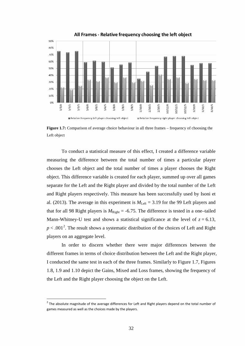
32
Figure 1.7: Comparison of average choice behaviour in all three frames – frequency of choosing the
Left object
To conduct a statistical measure of this effect, I created a difference variable
measuring the difference between the total number of times a particular player
chooses the Left object and the total number of times a player chooses the Right
object. This difference variable is created for each player, summed up over all games
separate for the Left and the Right player and divided by the total number of the Left
and Right players respectively. This measure has been successfully used by Isoni et
al. (2013). The average in this experiment is MLeft = 3.19 for the 99 Left players and
that for all 98 Right players is MRight = -6.75. The difference is tested in a one–tailed
Mann-Whitney-U test and shows a statistical significance at the level of z = 6.13,
p < .0012. The result shows a systematic distribution of the choices of Left and Right
players on an aggregate level.
In order to discern whether there were major differences between the
different frames in terms of choice distribution between the Left and the Right player,
I conducted the same test in each of the three frames. Similarly to Figure 1.7, Figures
1.8, 1.9 and 1.10 depict the Gains, Mixed and Loss frames, showing the frequency of
the Left and the Right player choosing the object on the Left.
2 The absolute magnitude of the average differences for Left and Right players depend on the total number of games measured as well as the choices made by the players.

33
Figure 1.8: Comparison of choice behaviour in the Gains frame –frequency of choosing the Left
object
Not surprisingly, Left players (average difference score of MLeft = 1.68) chose
the Left object more frequently than Right players (average difference score of MRight
= -8.38), Mann-Whitney-U z = 16.41, p < .001. In the Mixed frame, the average
difference score for Left players (MLeft = 3.5) and that for Right players
(MRight = -6.25) was significantly different as well, Mann-Whitney-U z = 16.41,
p < .001. Finally, in the loss frame Left players on average chose the Left object over
the Right object with a difference score of MLeft = 5.05 and Right players chose the
Right object over the Left object with an average difference score of MRight = -5.17.
The difference between these choices is also statistically significant, z = 15.63, p
< .001 (Mann-Whitney-U test).
5.1.2 Summary
Looking at the observed frequency ranges of all three frames as well as on
the aggregate level (Figures 1.7, 1.8 – 1.10), it can be stated that players tend to
overwhelmingly choose the object on their own side of the bargaining table. This
effect seems to be relatively robust. In absence of “the rule of closeness”, the most
effective choice for players would be to choose each disc with a probability of 50.0%
(Isoni et al., 2013). Thus, Hypothesis 1, which states that players use the spatial
distribution of the bargaining table and apply the “rule of closeness” in their

34
decisions, can be confirmed (i.e., the focal point is salient). The data further suggests
that the level of asymmetry and the framing influence the choice behaviour. This is
investigated in the following sections.
Figure 1.9: Comparison of choice behaviour in the Mixed frame – frequency of choosing the Left
object
Figure 1.10: Comparison of choice behaviour in the Loss frame – frequency of choosing the Left
object

35
5.2 The effect of asymmetry (α ≠ β, where α ≤ β)
In my experiment setup, I used different parameters for α and β creating
payoff-asymmetries. In this section, I test the impact of asymmetries on the choice
behaviour of the players and expected coordination rates.
5.2.1 Choice behaviour
Figure 1.11: Choice behaviour: frequency of the Left and the Right players to choose the focal point
Hypothesis 2. First I investigate the effect of payoff asymmetry on choice
behaviour. Figure 1.11 depicts the relative frequency for players to choose the focal
point by game (x-axis depicts value combinations for α and β). For example, the
(5, 5) data point includes the choice behaviour from the games α = 5, β = 5 and c = 0,
1, 5 across all frames. For this particular data point, the relative frequency for the
The frequency for both players to choose the focal point is thus 76.2% depicted by
the blue line. The red line depicts the expected coordination rate, in this case 63.7%
and the yellow line depicts the expected coordination rate on the Near equilibrium
(58.0%). Figure 1.11 shows an effect of asymmetries on choice behaviour. As the
level of asymmetry increases, the power of the relative frequency of focal point play
decreases.

36
Grouping the games according to the absolute difference between α and β,
which can assume the values 0, 1, 2, 5 and 9, the choice behaviour of the Left and
Right players choosing the focal point can be compared with a binomial test. Testing
the proportions of focal point play for each of the difference levels between α and β
against the proportion from the symmetric game (76.2%), the differences are
statistically significant (ps < .01). Thus, introducing asymmetry clearly reduces focal
point play at all levels of asymmetry.
Further, Figure 1.11 shows that spatial proximity has a different effect on
Left and Right players under asymmetry. For the Left player, the frequency of
choosing the focal point lies between 44.7% and 67.8% in the asymmetric games,
while the higher the asymmetry, the lower the observed frequency. For the Right
player, the range is between 65.9% and 67.7%. This suggests that the power of the
focal point decreases for the Left player as asymmetry increases, while the Right
player’s choice is unaffected. However, Figure 1.11 does not reveal whether the
choice behaviour of the Right player is influenced by the focal point (Near) or a
payoff bias. To further investigate the choice behaviour, I test players’ choices
against the theoretically predicted Nash equilibrium probabilities with a binomial test.
The differences to the observed frequency of choosing the focal point for the Left
player was significant (ps < .001). However, the same test for the Right player is
only significant for the α = 5, β = 5,6 as well as the α = 3, β = 8 game (ps < .01).
Given that the Nash equilibrium probabilities are calculated without the concept of
focality, the power of the focal point cannot be demonstrated for the Right players’
choice in half of the games (i.e., it cannot be determined whether the Right player’s
choice has a label bias).
Lastly, in this section I analysed the effects of increasing payoff-asymmetry
and player type (Left vs. Right) on focal point play (i.e., Near choices) with a
repeated-measures logistic regression that controlled for clusters in observations.
This analysis revealed that increases in payoff-asymmetries significantly reduced
choices of the Near equilibrium, odds ratio = .810, z = -5.21, p < .001. The effect of
player type was not significantly predictive of focal point play (p = .871), however a
significant interaction between asymmetry and player type supported the notion that
the increasing asymmetry influenced the Left and Right players differently, odds
ratio = 1.10, z = 3.61, p < .001. Specifically, whereas choosing the focal point was
not influenced by payoff-asymmetry for Right players, Left players chose the focal

37
point less often as payoff-asymmetries increased. Overall the results in this section
partially support Hypothesis 2 and show a payoff bias in players’ decision making in
most games.
5.2.2 Coordination
Figure 1.12: Expected Coordination Rate – Gains Frame
Figure 1.13: Expected Coordination Rate – Mixed Frame

38
Figure 1.14: Expected Coordination Rate – Loss Frame
Hypothesis 3. In this section I analyse the effect of payoff asymmetry on the
expected coordination rates. Figures 1.12, 1.13 and 1.14 depict the expected
coordination rate as well as the theoretically predicted rate for successful
coordination on the two pure Nash equilibria (P(S)) for the Gains, Mixed and Loss
frames. In order to analyse the impact of the level of asymmetry, I compare the
overall expected coordination rates of games grouped by their β – α values. For that I
grouped games with the same β – α values over all treatments and level of c. I first
compare the coordination rate of the games with β – α = 0 to games with β – α = 1.
Across all three frames, the range of expected coordination for the symmetric games
(α = 5, β = 5) is between 58.4% and 67.6%. The average over all games is 63.7%.
For the (α = 5, β = 6) games, the range of expected coordination is between 51.2%
and 56.2% and over all games the expected coordination rate lies at 53.2%. This
drop in coordination rate is statistically significant (χ²-Test, p = 0 .011). The games
(α = 3, β = 8) and (α = 5, β = 10) lie in the category of β -α = 5. Over all frames the
game (α = 3, β = 8) has an expected coordination rate of 51.9% and the games with
(α = 5, β = 10) lie at 52.3%. This difference is not statistically significant (χ²-Test,
p > .90). Compared with β – α = 1 games, the expected coordination rate did not
significantly drop (χ²-Test, p > .90). I omitted the analysis of the games on the
category of β -α = 5 as these games have a range of expected coordination rates
between 50.0% and 63.0%, which is a larger range than the (α = 5, β = 6). Lastly,
games in the category of β – α = 9 have an overall expected coordination rate of

39
48.2%. The difference to games in the category of β – α = 1 is also not significant
(χ²-Test, p > .10). Hence, expected coordination rates do not significantly decrease as
β – α increases, however, they decrease in comparison to symmetric games.
Figures 1.15, 1.16 and 1.17 depict the expected coordination rate of the Near
and Far equilibria for the Gains, Mixed and Loss frames. The figures generally show
that the coordination on the Near equilibrium is much higher than the coordination
on the Far equilibrium. The coordination on the Near equilibrium seems highest in
the symmetric games as well as the games with low payoff-differences (α = 5, β = 6),
(α = 10, β = 12). As payoff-differences increase (α = 1, β = 10), (α = 3, β = 8) and
(α = 5, β = 10), the difference between the coordination on the Near equilibrium and
the Far equilibrium diminishes. As payoff-differences become larger, the
coordination on the Near equilibrium decreases and the coordination on the Far
equilibrium increases. Thus, with an increasing payoff-difference, the power of the
focal point decreases. If these groups of games with low payoff-asymmetries and
high payoff-asymmetries are aggregated and compared, the difference is significant
(χ² = 13.66, p < .001). When payoff-asymmetry increases, coordination on the Near
equilibrium decreases. Overall, findings lend some support to Hypothesis 3.
Figure 1.15: Expected Coordination Rate (Near & Far Equilibrium) – Gains Frame

40
Figure 1.16: Expected Coordination Rate (Near & Far Equilibrium) – Mixed Frame
Figure 1.17: Expected Coordination Rate (Near & Far Equilibrium) – Loss Frame
5.2.3 Summary
The degree of asymmetry between α and β seems to have some effect on the level of
the expected coordination rate. Asymmetry lowers the expected coordination rate in
comparison with symmetric games. The degree of differences in α and β in
asymmetric games is not statistically significant. In addition, it can be observed that
an increasing payoff-difference across all frames descriptively weakens the power of
the focal point. The less favoured Left player chooses increasingly the Right object
with a growing payoff-difference, depending also on the absolute level of α and β.

41
The favoured Right player seems unaffected by the payoff-asymmetry. In aggregate,
this leads to lower focal point play across all players. Hypothesis 2 and 3 are
partially confirmed.
5.3. The framing effect
In section 5.3, the framing effects are examined, i.e. the comparison of all 18
games with the corresponding sets of parameters of α, β and c in the Gains, Mixed
and Loss frames (Δ = 0, -5, -10).
5.3.1 Choice behaviour
Hypothesis 4. In this section the influence of the framing effect on the choice
behaviour of the players is examined. It quickly becomes apparent that loss aversion
has an effect on the coordination behaviour of the decision-makers – however the
impact is quite different for the favoured (Right) and the less favoured (Left) player.
Figure 1.18 shows the average frequency of Left and Right players choosing the Left
object across all games, comparing the average results from the Gains, Mixed and
Loss frames.
Comparing the average of all 18 games across all three frames, an increase of
Left players choosing the Left object can be observed, which constitutes a framing
effect. As the variable Δ decreases, Left players seem to choose the near option more
often. In the Gains frame 54.7% of the Left players choose the Left object (Near),
while 59.7% choose that option in the Mixed frame and 67.0% in the Loss frame
(Figure 1.18). The increase from the Gains to the Loss frame is statistically
significant (χ² = 18.3, p < .001).
The increase from the Gains frame to the Mixed frame is marginally
significant (χ² = 3.23, p = .07), while the increase from the Mixed to the Loss frame
is significant (χ² = 6.14, p < .05). Across all frames, the difference of choosing the
Left and Right objects for the Left player is statistically significant, ps < .05.
Looking at all 18 games individually, a clear treatment effect cannot be
observed in every game. However, moving from the Gains to the Mixed frame and
from the Mixed to the Loss frame, in 14 out of 18 games a percentage increase of
Left players choosing the Left object could be observed (see Figure 1.19).

42
Figure 1.18: Average frequency of Left and Right players choosing the Left object across all
frames
Comparing the Gains frame with the Loss frame, in 17 out of 18 games a percentage
increase of Left players choosing the Left object could be observed. Testing the
individual games of the Gains, Mixed and the Loss frames with a χ²-Test, the
increase of Left players choosing the Left object is statistically significant, p < .01,
for 12 of the 18 games.
The strongest framing effect for Left players choosing the Left object was
present in the group of games (α = 3 and β = 8,) with an average increase of 27.9%
(χ² = 14.41, p < .001) between the Gains and the Loss frames. The group of games
with α = 1 and β = 10 also shows a stronger framing effect with an average increase
of 12.7% (χ² = 2.83, p = .09). In the case of payoff-symmetry (α = 5 and β = 5), the
average increase of Left players choosing the Left object between the Gains- and the
Loss frames is 15.1%. For the other groups of games, the percentage increase of Left
players choosing the Left object is below 10%. In 4 out of 6 groups of games, the
percentage increase of Left players choosing the Left object is larger comparing the
Mixed frame and the Loss frame than comparing the Gains frame with the Mixed
frame. The analysis on an individual game level provides some evidence that, as
overall nominal payoffs become more negative, Left players have an increasingly
strong incentive to choose the Left object.

43
As the scale variable Δ becomes increasingly negative moving from the
Gains to the Mixed to the Loss frame, the Right players tend to increasingly choose
the Left object (Figure 1.18). Aggregating all games in the Gains frame, 26.7%
choose the object on the left, in the Mixed frame 32.6% of the Right players choose
the object on the left, and in the Loss frame this number increases to 36.4%. The
increase is statistically significant (χ² = 12.9, p < .01).
Figure 1.19: Comparison of choice behaviour in the three frames-Left players choosing Left object
Figure 1.20: Comparison of choice behaviour in the three frames –Right players choosing Left object

44
Comparing the differences of the Gains and the Mixed frames, the increase
is significant, χ² = 5.21, p < .05. The difference from the Mixed to the Loss frame
however is not statistically significant (χ² = 1.64, p = .19). This suggests that for the
Right player introducing losses as a framing effect has a statistical effect on choice
behaviour, but increasing losses further does not statistically change behaviour.
Similar to Figure 1.19 for the Left player, Figure 1.20 shows the difference of choice
behaviour for the Right player in each individual game across the Gains, Mixed and
Loss frames. The choice behaviour of the more favoured Right player shows that the
framing effect causes generally an increase in the choice of the Left object also on an
individual level. The more favoured (Right) player chooses more often the Left
object (Far) as a result of the framing effect on an aggregate and individual game
level. The difference across all frames is statistically significant using a χ²-test
(ps < .010) except for the (α = 1, β = 10, c = 0) game. Descriptively, a particular
trend in Figure 1.20, cannot be established. Overall there is only partial evidence to
support Hypothesis 4 as only Left players choose the Near option more often, while
right players seem to choose the Far option more frequently when losses are
introduced. This suggests a payoff-bias in the choice behaviour as both players
choose the lower money amount when losses are introduced.
5.3.2 Coordination
Hypothesis 5. Next, I analyse the framing effect on coordination rates.
Considering the above choice behaviour of the Left and the Right player, it is not
surprising that the average expected coordination rate as well as the expected
coordination rate on the Near and Far equilibria do not show significant increases.
Figure 1.21 depicts the average coordination rate on the Near and Far equilibria. In
the Gains frame, the coordination on the Near equilibrium is 40.3%, while the
coordination rate on the Far equilibrium is 12.1%. Moving onto the Mixed frame, the
coordination on the Near equilibrium remains at 40.2%, while the expected
coordination on the Far equilibrium is 13.1%. These figures are intuitive as both Left
and the Right players increasingly choose the Left object as losses increase. The
coordination on the Near equilibrium remains at the 40.0% level since the increase in
the observed frequency for the Left player choosing the Left object neutralises the
decreasing observed frequency with which the Right player chooses the Right object.

45
The same neutralising effect can be observed for the expected coordination rate on
the Far equilibrium. The increase of 1% is marginal and an effect resulting from the
method calculating the expected coordination rate3. Comparing the Mixed and the
Loss frame, the average expected coordination rate on the Near equilibrium is 42.6%
and the coordination on the Far equilibrium is at 12.0%. The increase in the
coordination rate of the Near equilibrium can again be explained by the change in
proportion of the Left player choosing the Left object and the Right player choosing
the Right object which do not neutralise each other in terms of the expected
coordination rate. Statistically, the marginal changes in the expected coordination
rates are insignificant (χ² = 0.57, p = 0.74).
Figures 1.21: Average expected coordination rates: across all frames, and average expected
coordination rate on the Near and Far equilibria across all frames.
Considering the expected coordination rates of the Gains, Mixed and Loss
frames as depicted in Figure 1.21, a marginal increase between the frames can be
observed. The Gains frame shows an expected coordination rate of 52.2%, while the
Mixed (53.4%) and Loss 54.6% frames show marginally higher expected
coordination rates. Testing with a χ²-test against the null hypothesis that the
3 For the “Near” equilibrium, this is the observed frequency of the Left player choosing the Left object multiplied with the observed frequency of the Right player choosing the Right object.

46
proportion of expected coordination compared with all pairs in a particular frame is
the same, the result shows that the null hypothesis cannot be rejected (χ² = 0.075,
p = .96). The observed increase of expected coordination rate is thus statistically not
reliable.
To investigate effects of different levels of α and β, I test the expected
coordination rate individually in all 18 games (Figures 1.12, 1.13, 1.14). Overall 13
games showed an increase of coordination rates comparing the Gains frame with the
Loss frame. The largest differences were observed in the games with a relatively low
α- value (Left object) and with a large payoff-difference (α = 3, β = 8) and (α = 1,
β = 10). The maximal increase in these two sets of games is 13.4% and 7.2%. On the
other hand for games with very large α-values (Left object) and low payoff-
differences, (e.g., α = 10, β = 12) a decrease of coordination rates has been measured
up to -9.97%. Differences are generally not significant (p > .05). When looking at
the expected coordination rates on the Near equilibrium (focal point), 14 games
showed increases comparing the Gains with the Loss frames. For the games (α = 3,
β = 8) and (α = 1, β = 10), the coordination on the Near equilibrium shows an
increase of expected coordination of up to 28.1% and 6.55% respectively.
Coordination on the Far equilibrium decreased on 10 games comparing the Gains
and the Loss frames. Comparing the Mixed with the Loss frames, it can be stated
that 12 games showed increasing expected coordination rates. The expected
coordination on the Near equilibrium shows an increase in 10 games. On an
individual game level, 3 games out of the group of α = 3, β = 8, c = 0,1 and α = 1, β
= 10, c = 1 as well as a game with symmetric payoffs showed significant increases
(χ²-test p < .05). Increases in the expected coordination rate were caused by
increases on the coordination rate of the Near equilibrium.
Keeping in mind that the strongest framing effects were found for the Left
players choosing the Left object in the (α = 3, β = 8 and α = 1, β = 10) games, the
increase in coordination on Near equilibrium can be explained. In the observed
games, the frequency of the right player choosing the Left object changed only
marginally. Overall, coordination rates do not show a significant improvement as a
result of the framing effect. On an individual game level some evidence of an
improved coordination rate is found. However, in total there is little evidence to
support Hypothesis 5.

47
5.3.3 Summary
Comparing the Gains, Mixed and Loss frames, a framing effect regarding the
choice behaviour of the Left and the Right players emerged from the data. On an
aggregate level, the Left and Right players were more likely to choose the Left
object as a result of framing. Looking at the 18 individual games, the effect of Left
and Right players increasingly choosing the Left object is found as well and is also
significant (13 games).
Comparing the expected coordination rate across frames, the expected
coordination rate marginally increases as a result of the framing effect; however,
statistically this is not significant. The effect of the Left and Right players
increasingly choosing the Left object leads to a neutralisation and the expected
coordination rate does not change. However, looking at each of the games across the
three frames, a significant increase of the expected coordination rate can be detected
caused by the strong increase of the Left player choosing the Left object and a
marginal increase of the Right player choosing the Left object.
Conclusively, I cannot confirm that expected coordination improves between
frames with increasing losses (Hypothesis 5). Further, the data do not confirm that in
light of increasing losses in the Gains, Mixed and Loss frames players would choose
increasingly the Near option (i.e. the focal point; Hypothesis 4). Further, for the Left
player, it cannot be determined whether the motive for choosing the Left object is
focality or a bias towards the low payoff.
5.4 The effect of cost c
In this section, I analyse the effect of the cost variable c on choice behaviour
(Hypothesis 6) as well as the expected coordination rate (Hypothesis 7). Proposition
1 predicts an increasing expected coordination rate with an increasing factor c.
Schelling’s (1960) reasoning as well as loss aversion theory would suggest that
players choose the label salient focal point more often in order to avoid coordination
failure.

48
5.4.1 Choice behaviour
Hypothesis 6. According to Hypothesis 6 players choose the Near option as a
result of potential losses from coordination failure. Figure 1.7 in section 5.1.1 depicts
the average choice behaviour of choosing the Left object across all three frames,
comparing the behaviour of the Left and the Right players. Left players chose the
Left object with a much higher frequency than the Right players. Further, Figure 1.7
shows that in aggregate, over all three frames the impact of c on choice behaviour for
the Left and Right players is rather small in games with a low difference between α
and β. The lower the value of α, and the higher the payoff-difference, the larger
seems the effect of the cost c. For the (α = 3, β = 8), (α = 1, β = 10) and the (α = 5,
β = 10) games, there seems to be a continuous increase of Left players choosing the
Left object for c = 0, c = 1 and c = 5. For the (α = 3, β = 8) game, the frequency
increases from 51.5% (c = 0) to 58.8% (c = 5). For the (α = 5, β = 10) game, the
increase is also rather small, from 55.1% (c = 0) to 57.7% (c = 5). Using a χ²-test,
these differences are not statistically significant (p > .10) and remain descriptive.
However, for the (α = 1, β = 10) game, the frequency increases from 35.1% (c = 0) to
45.4% (c = 1) to 53.6% (c = 5), and this difference is significant at the 5% level
using a χ²-test (χ = 6.785, p < 0.05). Looking at the frames individually, Figures 1.8,
1.9, and 1.10, choice behaviour can be observed in more detail, however mainly no
significant results were found. The choice behaviour of the Left player choosing the
Left object games can also be categorised into two groups - games with a low
payoff-difference and a large payoff-difference. In the Loss frame (Figure 1.10) for
the (α = 1, β = 10), game players chose the Left object with 35.7% for c = 0 and with
67.9% for c = 5. This increase is significant at the 5% level (χ² = 5.81, p < 0.05).
Regarding Figure 1.7, for the Right player in most games no significant
difference in choice behaviour could be observed with an increasing cost of c. In
four groups of games in aggregate, Right players chose less frequently the Left
object when comparing games with c = 0, c = 1 and c = 5. In three groups of games
that frequency dropped when comparing the games of c = 0 and c = 5. Notably in the
group of games with (α = 1, β = 10) 32.5% of Right players chose the Left object for
c = 0, 25, 8% for c = 1 and 41% for c = 5. The overall difference in choice is
marginally significant using a χ²-test (χ² = 5,31, p < 0.07). The games in each of the

49
individual frames as depicted by Figures 1.7, 1.9 and 1.10, show no statistical
significance in the choice behaviour of the Right player (p > .10).
Also, I tested whether the probability of focal point play depended on both
losses and player type (Left vs. Right). Binomial tests revealed that the probability of
focal point play increases for Left players as losses increased. Specifically, for Left
players, the probability of choosing the Left object increases from 51.5% to 58.8% as
c increases from c = 0 to c = 5, a significant increase as shown by a binomial test,
p < .010 (one-tailed). The difference in probability between c = 1 and c = 0 was in
the predicted direction but not significant (p > .19, one-tailed). However, focal point
play was largely unaffected by increases in losses for Right players, ps > .50. This
suggests that increases in observed coordination are primarily due to the Left players
choosing the Left object more often as losses increased.
Elucidating the above result, I tested whether increases in cost c predict
overall salient focal point play (Near, Near). I used a repeated-measures logistic
regression while controlling for player type (Left vs. Right). The regression
confirmed that increasing the cost from c = 0 to c = 5 predicted more choices with
regards to the focal point, odds ratio = 1.46, z = 2.11, p = .035. Hence the results in
this section partially support Hypothesis 6, such that increasing losses increase focal
point play. However, this seems to be primarily due to Left players choosing the
Near option more frequently.
5.4.2 Coordination
Hypothesis 7. According to Hypothesis 7, the overall coordination rate should
increase as a result of increasing costs c. As can be seen from Figure 1.22, the
expected coordination rate increases slightly from 52.7% to 54.3% as c increases and
coordination failure becomes more expensive. However, a χ²-test of the expected
frequency of coordination revealed no significant difference between the expected
coordination rate in the three loss conditions, (χ² = 0.12, p > 0.94). Further, the
overall expected coordination rate on the Nash equilibrium (Near, Near) increases
slightly as losses increase. However, a χ²-test revealed that this increase was also not
significant, χ² = 0.59, p > .74.

50
Figure 1.22: Expected coordination rates across all frames; Expected coordination rates on
the Near and Far equilibria.
Figure 1.23: Expected coordination rates across all frames for the individual games.
A more detailed analysis of each individual game confirms the above result.
The blue line in Figure 1.23 depicts the expected coordination rate across all games
(x-axis depicts value combinations for α, β and c). The changes are not significant
for any group of games (ps > .68). Also, the changes within each group of games
(e.g., the α = 5, β = 5 set of parameters with c = 0, 1 and 5) of the expected
coordination rate for the Near and Far equilibria do not show significant changes
(ps > .67).

51
Finally, an analysis of the individual framing conditions revealed (Figures
1.12-1.14) that the games do not show any significant changes in terms of expected
coordination rate (Gains frame ps > .77, Mixed and Loss frames ps > .89). Overall
the data do not seem to be support Hypothesis 7.
5.4.3 Summary
The cost factor c has an impact on choice behaviour for the less favoured Left
players in games with a large payoff-difference. For the favoured Right players
raising the cost factor c does not yield a clear effect. Four of the 6 groups of games
yield an increase of the focal point choice comparing c = 0 and c = 1. This provides
partial evidence in support of Hypothesis 6. The impact of c on the expected
coordination rate is statistically insignificant. An improvement of coordination rates
can be measured for games with a large payoff-difference. At the aggregate level, a
continuous increase of the expected coordination rate can be observed in the (α = 1,
β = 10) games, which have the highest difference in payoffs. The results from the
individual frames confirmed this result. Overall there is not sufficient evidence to
support Hypothesis 7.
6. Conclusion & discussion
The research presented in this chapter investigates the effect of losses in
symmetric and asymmetric battle of the sexes games. In order to adequately address
this question, I used a series of 18 two-player coordination games. Players were
randomly placed on the left and right side of a bargaining table. The games were
presented to the subjects with six different symmetric and asymmetric payoff-
combinations, in which a higher payoff was always presented on the right side of the
bargaining table. Each of the six payoff-combinations was paired with a cost level c,
which represented the coordination failure payoff. Cost level c had three different
values (c = 0, 1, 5). Some games were framed differently by subtracting a scale
variable Δ from all game payoffs. The scale variable had three values (Δ = 0, -5, -10)
constituting the Gains, Mixed and Loss frames. In the Mixed frame, game payoffs
presented were partially positive and partially negative. In the Loss frame, game

52
payoffs were negative or zero but never positive. This design enabled testing
whether negative payoffs and potential losses impacted players’ decision-making.
The different levels of asymmetry allowed to better measure the use of the “rule of
closeness” which constituted the label-salient focal point in these games (Schelling,
1960).
Prospect theory and loss aversion in particular suggest that players will more
strongly prefer to avoid a certain loss rather than making an equivalent gain. My
experiment setup presented in this chapter provided a possibility for players to make
use of strategy labels (i.e., the “rule of closeness”) in order to cooperate and avoid a
loss. An increase in coordination in games with losses, as well as an increasing
number of players’ choosing the label-salient focal point across all games was
expected.
The results of the experiment (Isoni et al., 2013) demonstrated that in absence
of the Left and Right spatial distribution, players coordinated less. In their design,
the objects were placed in the central area of the bargaining table, such that for both
players the distance to the objects was exactly the same. The salience of the focal
point is an integral part of the experiment design as in absence of or a weakly salient
strategy label would force players to randomise between their choices.
The first hypothesis was confirmed and players indeed used the power of the
focal point by overwhelmingly choosing the object that is closest to them. This
finding is in accordance with other works such as Schelling (1960), Mehta et al.
(1994a), Crawford (2008), and Isoni et al. (2013) and suggests that the “rule of
closeness” is a salient focal point to the players. Furthermore, in my experiment
setup, this strategy provides an option to avoid a loss.
In terms of increasing payoff-asymmetry, research shows that the power of a
strategy label is diminished (Crawford et al. 2008). Isoni et al. (2013) contended that
label salience is still powerful in asymmetric games and that the degree of salience
strongly depends on the framing of the experiment. In comparison to Isoni et al.
(2013), my experiment was not focused on elucidating different framing aspects of
asymmetric bargaining games. My experiment setup presented in this chapter uses
just one particular type of spatial distribution. However, as in Isoni et al. (2013) and
Mehta et al. (1994a,b), my experiment uses the “rule of closeness” as a label-salient
strategy.

53
My findings suggest that asymmetry influences the Left and Right players
differently. Less favoured Left players chose with increasing asymmetry of the
payoffs, ceteris paribus, more often the more valuable object on the right. This also
corresponds with the findings of Crawford et al. (2008), where players favoured the
high payoff in games with high asymmetries. The data from my experiment showed
that the more favoured player was largely unaffected by the increase in asymmetry
(i.e., also in games with a low payoff-asymmetry, the Right player chooses the object
on the right). As in Crawford et al. (2008), when label salience contradicts payoff
salience, players do not coordinate. The work of Crawford et al. (2008) reported that
with low payoff-asymmetries, both players favoured the payoff of the other player
leading to coordination failure.
The choice behaviour of the Left player thus implies also a clear payoff-bias,
as the object on the right with the potentially higher payoff is more frequently chosen
as potential losses increased. However, the player on the right remains unaffected by
increasing asymmetry. Nonetheless, it is difficult to speculate whether the choice is
unchanged because of the power of the focal point or because of a payoff-bias by the
decision-maker. In my experiment setup, the strategy label and the higher payoff are
mutually reinforcing. Another possible explanation is that players were influenced
by the possible losses. Overall, there is some evidence to support Hypothesis 2, such
that increasing payoff asymmetry can lead to a stronger payoff bias.
Given the simple choices in my experiment, the findings presented in this
chapter regarding the effect of asymmetry partially correspond with Nash
equilibrium theory. However, the absolute level of expected coordination decreases
with the increasing level of asymmetry only descriptively. Compared with
symmetric games the expected coordination rate is significantly lower. Hence,
evidence partially supports Hypothesis 3. Compared with Crawford et al. (2008), the
expected coordination rate is slightly higher, however not significantly so and might
be due to the different framing of the two experiments.
Considering the differences across the Gains, Mixed and Loss frames, the
findings of my experiment present new insights into the use of focal points. Against
the expectation that players would make use of the label-salient focal point (i.e., the
“rule of closeness”), it was observed that both players were significantly influenced
by the framing effect such that they increasingly chose the less valuable object on the
left. For the Right player, this means that as losses increase the power of the label-

54
salient focal point diminishes due to a clear payoff-bias. This finding suggests that
loss aversion induces a payoff-bias into the decision-making process of the more
favoured player, making him choose the lower payoff in order to avoid the looming
loss. For the Left player it cannot clearly be discerned whether the decision stems
from a label or from a payoff-bias.
One possible way to examine the data would be a Level-K model as
presented in Crawford et al. (2008). However, there are several drawbacks of using
such a model. Differently to Crawford et al.’s (2008) X-Y game experiment, the
current games were no one-shot games but presented in a sequence to the subjects. In
this way, a Level-K model needs to be tested to ensure that it can be used to explain
the data. Additionally, in the assumptions of Crawford et al. (2008), the percentage
of level 0 thinkers is presumed to be zero. Informal analysis of the questionnaire at
the end of my experiment suggests otherwise. I conjecture by looking at the
cumulated behaviour of the Left and the Right player, that loss aversion creates a
preference for the lower payoff for both players. This would suggest that the strategy
label of the focal point does not influence the decision-makers as a result of losses
being present. The behaviour suggests that in light of loss aversion, players forgo the
possible high payoff and rather attempt to prevent the loss by voluntarily taking the
lower payoff.
This in turn leads to marginal differences of the expected coordination rate
across the three frames, as both players increasingly chose the Left object and thus
the lower payoff. In certain instances with a high payoff-asymmetry, the Left bias for
the Left player is particularly strong, such that the expected coordination on the Near
equilibrium increases drastically, and also the overall expected coordination rate. A
high payoff-asymmetry makes the low payoff more salient, as players recognised the
low payoff as a viable strategy in order to prevent a loss. Additionally, payoff-salient
choices do not necessarily influence the overall coordination rate. Hence, in
summary there is little evidence to support Hypotheses 4 and 5.
The effect of the cost c on players’ choice behaviour reveals a similar effect
as the framing manipulation. Again, for the Left player a Left bias can be observed,
however only in games with a high payoff-difference. The choice behaviour of the
Right player is statistically not affected by the cost. Overall, however, analyses
showed cost c is a good predictor for choice behaviour.

55
Higher payoff-asymmetries as well as higher losses might have increased
statistical significance of the Left bias. Another possible explanation for the results
might have been sample size. Regarding the expected coordination rate, no
significant results can be reported. Descriptively, we find the same tendencies as in
the framing condition. As c is a significant predictor of choice behaviour, results
suggest that at least Left players exhibit a Left bias in their choices. Given that the
effect of the cost c is rather weak on the Right player, it cannot be concluded with
certainty what the underlying motivation is for the Left player choosing increasingly
left. In summary, the evidence on focal point play and overall coordination do not
fully support Hypotheses 6 and 7.
I conclude that the results clearly show losses have an effect on players’
choice behaviour. Loss aversion creates a preference for choosing the lower payoff
for both players as a “safe strategy”. In light of the evidence, it can be concluded that
losses do not strengthen the salience of the label-salient focal point. As a result of
choice behaviour, the expected coordination rate is mainly unaffected by increasing
losses. Overall, the losses in the Loss frame seemed salient to the players while the
cost c did not have an effect with the same magnitude. The findings from my
experiment bring to light that losses in an interactive coordination game do not
necessarily improve coordination, as players do not regard label salience as a
determinant in their decision-making process. However, losses seem to establish a
payoff-salient focal point (i.e., the low payoff-object). In a coordination game with
losses, the power of the label-salient focal point seems to be weakened, contradicting
Schelling’s (1960) theory about focal points. The results show that losses in a
bargaining scenario induce readiness to compromise regarding the division of the
pie.
Future research should attempt to explain the preference of players for the
lower payoff by focusing on games with large payoff-asymmetries and higher costs
for coordination failure. The potential payoff-bias should perhaps be investigated
with a cognitive hierarchy model. Also, in order to make losses more salient, it is
recommended to introduce real losses into the experiment setup. This could be done
in a field experiment, such that the salience of losses can be observed in a more real
environment. Further, it should be investigated whether these findings extend to an
interactive alternating offer bargaining scenario, such that it is possible to observe if
players do compromise more. Also, a similar experiment should be conducted in

56
which the focal point “rule of closeness” is replaced with a perhaps even more label-
salient focal point.

57
Chapter 2 The Effect of Culture and Self-Interest on Intercultural Bargaining Games
1. Introduction
Given the globalization of the world’s economies, intercultural negotiation
processes, haggling and bargaining efforts are becoming increasingly complex
phenomena. For that reason, economists alongside other scientists have attempted to
explore the deeper meaning of intercultural behaviour and bargaining outcomes. As a
consequence, there is a crucial need to understand the role of “culture”. Bargaining
experiments have shown that different cultural groups can substantially differ in their
bargaining behaviour, which affects bargaining offers and outcomes (Henrich, 2000,
Henrich et al. 2001, Croson et al., 1999, Roth et al., 1991, Ferraro & Cummings,
2007– henceforth FC, Gurven et al. 2008, Chen & Tang, 2009).
In various fields of science, cultural effects in bargaining situations have been
well documented. Management studies have shown a drop of the joint bargaining
surplus of up to 25% in intercultural bargaining situations compared to intracultural
bargaining settings (Brett & Okumura, 1998; Adler & Graham, 1989; Adair et al.,
2001). For example, some of these experiments measured the bargaining behaviour
of Japanese and American managers in complex multi-issue negotiations. These
researchers attempted to attribute the drop in bargaining efficiency in intercultural
settings as a function of individualism, information, trust and communication. A
recent study was conducted by Hofstede et al. (2012) to examine culturally
differentiated behaviour using a model based on an ABMP4 negotiation architecture.
Hofstede et al. (2012) found that culturally differentiated behaviour can be generated
according to their cultural model (Hofstede, 1984, 2001 - the combined works are
hereafter denoted as HS).
4 ABMP – Agent-Based Market Place negotiation as defined by Jonker & Treur, 2001. In this model agents are able to use any given set of incomplete information along with “guessing” the other player’s preferences based on past negotiations to improve the overall bargaining outcome in a one-to-one, cooperative, multi-issue bargaining situation.

58
While cultural differences have been examined extensively in different
scientific fields, the topic has not yet been widely investigated in the field of
experimental economics, bargaining and game theory. In recent times, the trend in
game theory has shifted towards researching non-pecuniary aspects such as
determining factors of game theoretic and bargaining outcomes (Camerer, 2003).
Researchers from several different disciplines have been interested in studying the
development, interaction and inefficiencies (e.g. difficulties in communicating
properly as well as acting in conflicting ways in any arbitrary situation) of
intercultural bargaining. Psychological games (Pearce, 1984), identity (Akerlof &
Kranton, 2000), or the role of fairness in economic games (Fehr & Schmidt, 1999;
Bolton & Ockenfels, 2000) do not sufficiently introduce the effect of values in a
strategic interaction, regardless of whether it may be of a social, political or business
nature. Standard bargaining theory of Nash (1950) and Rubinstein (1982) as well as
repeated bargaining situations as investigated by Muthoo (1999) do not consider
intercultural value systems as part of the bargaining process. Regarding international
and intercultural conflicts, game theory has for instance been employed for
investigating in coordination strategies, such as the Cold War in Thomas Schelling’s
‘The Strategy of Conflict’ (1960).
Emerging literature in experimental economics has started to focus on
several strands of research designed to explain the impact of culture on bargaining
behaviour and outcomes. Hennig-Schmidt et al. (2002) as well as Croson et al.
(1999) focus on bargaining power asymmetry as one of the causes for different
bargaining behaviour and outcomes in intercultural scenarios. Among others, Croson
et al. (1999) and Roth et al. (1991) mainly focus on intercultural differences in
bargaining outcomes. Chen & Tang (2009) investigate the impact of cultural traits
and religious beliefs on bargaining behaviour among culturally different groups in
China using a series of ultimatum games. This study concluded that the observed
difference in offer and acceptance rates among the different groups were attributable
to differences in culture. Further research focused on discrimination as a main
determinant of an intercultural influence on bargaining (Barr & Oduro, 2002, FC).
The latter work focused on two distinct cultures living in the same space in an
industrialized society. While controlling for demographic differences in the subject
pool, this study used strategic ultimatum games to elicit beliefs, and it showed clear
differences in bargaining behaviour. In the ultimatum games, subjects were asked to

59
hypothetically split an amount of $10 and state where their offer and acceptance
levels were. This study showed that behaviour was subject to racial discrimination,
as players could observe which players they were bargaining with (i.e., whether there
were more players of their own ethnicity in the bargaining session or not). This
model further differentiated between “rational stereotyping” and “preference-based
discrimination” (FC). FC further contended that observed discrimination in
intercultural settings between the cultural groups involved can be generally split into
rational stereotyping or statistical discrimination (Arrow, 1973; Phelps, 1972) and
preference-based discrimination (Becker, 1971). Statistical discrimination describes
an agent’s behaviour as a reaction to average behaviour of another group.
Preference-based discrimination describes if an agent simply has the preference to
behave differently when interacting with an individual from a given group (FC). The
findings of FC show that even within the same society, two distinct cultures can
exert different bargaining behaviours based on mainly preference-based
discrimination.
Given the experimental studies across various academic domains, the
question arises whether the bargaining and cooperation process is more efficient in
terms of a joint surplus and rounds needed to reach an agreement in an intracultural
setting compared to an intercultural setting (FC). Also, in terms of bargaining
outcomes, one particular set of culture-based preferences might provide a systematic
advantage in the bargaining process (Maynard-Smith, 1982). In order to shed light
on these issues, it might be helpful to include preferences based on cultural values
and cultural background into the bargaining process. This makes it possible to
construct an adequate model for predicting bargaining outcomes as well as strategic
interaction in intercultural scenarios and to establish the key parameters and forces
involved in that process. The above-mentioned research mainly uses circumstantial
evidence to highlight intercultural effects (e.g., Chen & Tang, 2009). Previous
research often attributes the difference in behaviour between people from different
countries to the differences in culture, but fails to acknowledge particular social
preferences that underlie a particular behaviour (Oosterbeek et al. 2004).
Contributing to existing research, this chapter focuses on whether nationality
and corresponding levels of individualism determine the level of self-interest and
bargaining behaviour among the subjects. In the current experiment presented in this
chapter, I measured offer and acceptance rates in a series of ultimatum and

60
alternating offer games using a direct response method, in combination with a
measure of self-interest. Also, my experiment was designed to show whether
different levels of individualism and self-interest lead to significantly different levels
of payoffs, and thus might have a systematic strategic advantage as a result of their
cultural background and corresponding level of self-interest.
For the purpose of my experiment, other possible determinants of decision-
making were not considered. Putting the focus on simple ultimatum and alternating
offer games rather than complex negotiation procedures allows me to measure the
bargaining behaviour of the two involved distinct cultural groups.
The remainder of this chapter is structured as follows. In the next section, I
discuss cultural implications of my experiment. Section 3 outlines the recruiting,
design and procedure of my experiment. Section 4 states the expected hypotheses. In
Section 5, I discuss the results and experiment findings. A discussion in Section 6
concludes. Theoretical implications of the experiment are considered in Appendix
2.1 and 2.2.
2. Culture
Across various academic fields (including anthropology, sociology, business
and management studies) as well as economics, a consensus regarding the
terminology of culture has been reached, establishing that culture and cultural values
are learned and shared by a large group of people (e.g., HS, Hoecklin, 1995).
Samovar & Porter (1985) defined culture as a deposit of knowledge, values,
hierarchies, religions and concept of the universe acquired by a large group of
people. The anthropologist Kluckhohn (1951) stated: “Culture consists of patterned
ways of thinking, feeling and reacting, acquired and transmitted mainly by symbols,
constituting the distinctive achievements of human groups, including their
embodiments in artefacts; the essential core of culture consists of traditional ideas
and especially their attached values” (Kluckhohn, 1951 – p.86). In order to explain
the impact of culture and cultural values on intercultural bargaining, I conjecture that
it would be necessary to devise a cultural model that explains the impact of religion,
outside forces, societal norms and its derivations and consequences on intercultural

61
bargaining separately. The complexity of the issue can be best shown by Hofstede’s
(2001) diagram of stabilizing culture patterns (see Figure 2.1).
Figure 2.1: Culture Cycle according to Hofstede (2001)
An important conclusion of Hofstede (2001) is the interdependence of forces
of nature, ecological factors, value systems and emerging institutions, all of which
should be investigated separately for the purposes of economics in order to make
accurate predictions. In everyday life, the visible manifestations of culture are
practices, such as symbols, following leaders and performing rituals. Thompson &
Hickson (2002) defined the values of a society as stemming from the existence of
heroes and their social reactions, which are emulated by the population in order to
enhance the self-image.
A more comprehensive view of culture is largely based on the work of HS,
where the learning of culture is described as mental programming. This refers to a
fixed set of routines being physically determined by the state of our neural circuitry
and not directly observable, yet aiding in the predictability of behaviour. The work
by HS mainly focused on cultural dimensions in societies, meaning the systematic
circumstances that define a particular society (e.g., institutions, values and the
framework of mental programming). HS did not necessarily explain the resulting
behaviour and preferences of an individual from a particular society. Culture in this
instance, can only be measured as a statistical average of a larger group. HS
OUTSIDE INFLUENCES Forces of nature Forces of man: Trade Domination Science
ORIGINS Ecological factors: Geography History Demography Hygiene Nutrition Economy Technology Urbanization
SOCIETAL NORMS Value systems of major groups of population
CONSEQUENCES Structure and functioning of institutions: Family patterns Role differentiation Social Stratification Socialization Educational systems Religion Political Systems Legislation Architecture Theory and development
reinforcement

62
described culture as a five dimensional model with the dimensions of power
distance, individualism, masculinity, uncertainty avoidance as well as long-term
orientation. Power distance describes how less powerful members of a society accept
the fact that power is distributed unequally. Individualism is defined as the degree of
interdependence (or independence) between the members of a society. Masculinity
defines to which degree people act as achievers and wanting to be best-in-the-field.
Uncertainty avoidance is defined by how people deal with unknown and ambiguous
situations. Long term orientation measures whether a society is able to hold a
pragmatic future-oriented perspective. In order to understand the culture of a society
in Hofstede’s dimensional model in a holistic way, all five dimensions are necessary.
Other research has been conducted regarding culture and the effects of
cultural differences on bargaining. In their study on negotiation, Brett & Okumura
(1998) used the cultural dimension model of Schwartz (1994), exerting that it is
superior to that of HS. Schwartz (1994) used seven categories of cultural values,
namely Conservation, Hierarchy, Intellectual Autonomy, Affective Autonomy,
Competency, Harmony and Egalitarian Compromise. Conservation defines the
preference for conformity and traditionalism. Hierarchy outlines the preference for
fixed hierarchical roles. Intellectual Autonomy describes values that define a person
as its own entity – independence. Affective Autonomy is synonymous with pleasure
seeking. Competency comprises the values for success and a varied life. Harmony
defines a harmony with nature. Lastly, Egalitarian Compromise is the value set
which values the wellbeing of others. The work of Schwartz (1994) criticized the
mere focus of individualism versus collectivism in terms of cultural dimensions.
Researchers over the years have developed several other approaches regarding
cultural modelling (Triandis 1995, Triandis & Gelfand 1998). Some research does
not focus on cultural dimensions but on resulting behaviour such as communication
(FC).
Although some consistency exists in the terminological use of “culture”, the
concept itself seems to be difficult concept to grasp for social scientists and many
different approaches of defining it exist. Generally, it can be stated that it is almost
impossible to obtain a complete picture of all cultural aspects along with
corresponding value systems and resulting behaviours in a single experiment. In
cultural terms, the experiment of the current chapter focuses on the presumed
difference in culture background and corresponding social preference level of self-
63
interest with regard to origin and nationality. For the purpose of my experiment,
Eastern and Western cultures are grouped by the corresponding individualism scores
from Hofstede’s five dimensional model (HS). This view has been the most widely
adopted and researched definition of cultural differences (Hofstede 1980).
There is a particular statistical variance of preferences in each cultural group
(HS). Hence, people in general do not automatically have the same preference
pattern.. In my experiment, however, despite the relatively small sample size for the
purposes of measuring cultural phenomenon, I assumed that subjects on average
behave according to their cultural background. FC phrased this general idea as the
“statistical distribution of beliefs, values and modes of thinking that shape behaviour
among a group of people (e.g. notions of fairness)” (FC). For the purpose of my
experiment, I adopted the above-stated definition by FC regarding culture.
In my experiment, I measured the level of self-interest, and tested if there is a
correlation to the level of individualism as defined by HS. The distinction between
individualism and self-interest is an important one. According to HS’s (2001)
dimensional model, an individual from an individualistic culture is self-focused
rather than focused on the collective of society. However, the level of individualism
does not necessarily predict a certain level of self-interest. For example, a collectivist
person, focusing on the larger group rather than on one-self, might do this out of
self-interest if the group-orientation yields him the larger payoff. This distinction
between the level of individualism as well as self-interest is an integral part of my
experiment. Past research (Brett & Okumura, 1998, Adair et. al, 2001) showed that
individuals focusing on themselves tend to be more self-interested. The underlying
assumption implied by Hofstede (2001) is that the level of self-interest, similarly to
fairness, is a behaviour or social preference directly related to an underlying cultural
set of values. My experiment aims to investigate bargaining behaviour and outcomes
in relation to the cultural trait of individualism as well as self-interest.
3. Experiment
3.1 Recruiting
The overall aim was to create two distinct subject pools consisting of
subjects with a different level of individualism as defined by HS. The work of HS is
64
based on cultural surveys that were conducted in different countries. Hofstede
measured scores in each country (more than 50 countries) for his proposed 5
dimensions (power distance, masculinity, uncertainty avoidance, long term
orientation and individualism). These scores describe the average preference of the
citizens of a particular country regarding problem solving, decision making and
overall behaviour. For example, an individualism score of a particular country, thus,
describes the average preference and predisposition of the people for making
independent decisions and acting independently. A high score means that subjects
from that country behave, on average, individualistically (i.e., do not prefer the
group influencing their decision making, problem solving and considerations). For
two nations to have similar set of cultural preferences and values in terms of HS, all
five scores need to be similar. In such a case it can be conjectured that people would
have similar preferences and are more similar in their decision making compared to
countries in which the scores are divergent.
In the current study I focus on the degree of independence of subjects (i.e.,
individualism) as this dimension influences bargaining the most (Brett & Okumura,
1998). Typically experiments in the literature compare bargaining behaviour of two
distinct nationalities or particular ethnic groups within a country. Due to a limited
number of international students at the University of East Anglia I grouped countries
with a similar IDV-score from which I recruited subjects. Other dimensions in terms
of the HS model were not considered, as it would have not been possible to find
countries for which all scores are similar, and to then find sufficient subjects from
these countries. Hence, the countries were selected according to two criteria. I first
looked at the IDV-score (individualism score) of Hofstede’s 5 dimensions model
(HS). I chose countries for my sample in a narrow score range. One group of
countries selected had an IDV-score5 of 20-25 on a scale from 1 to 100 with 100
being the highest score. Other group of countries selected had scores between 80 and
91. Second, to refine the first selection of countries I considered the cultural and
socio-political heritage (HS).
The main part of the subject pool belonged to either the UK or China. The
dimensional scores of China and the UK as stated by HS can be compared to better
5 Different IDV (individualism) country scores are taken from Hofstede (2001) and can also be reviewed on the website of the Hofstede center at geert-hostede.com.

65
understand the subject sample. China has a power distance score of 80 whilst the UK
has a score of 35. This means that subjects from China should be more accepting of
the fact that power is distributed unequally. Both countries have a masculinity score
of 66, meaning that competition and success is equally important. Both countries
have a similar uncertainty avoidance score (China 30 and the UK 35), meaning that a
similar level of competition and drive to win exist. The countries have a divergent
score with regard to long term orientation (China: 87, UK: 51), meaning that people
from China are more pragmatic than the people from the UK. This allows Chinese
individuals to adopt long standing traditions and values more easily to a new
situation. Most importantly, the individualism score is also divergent (China 20, UK
89), meaning that Chinese individuals are supposed to be more group oriented on the
average, while UK citizens are more individualistic. As described, when recruiting,
the IDV-score was used as decision criterion.
The largest student group with a high IDV-score were British students. This
group was named the Western group as the UK is geo-politically part of the Western
world. In order to increase the subject pool in this group, subjects from the US,
Canada and Australia were recruited, as these countries were former colonies of
England and share to a large part language, religion, traditions, beliefs and socio-
political heritage (HS). This group of nations scored in the high range in terms of
IDV-score. Similarly, the highest number of subjects from the group of countries
with low IDV score was available from China. In order to increase the subject pool
for my experiment I chose other countries with a similar IDV-score as well as with a
historical cultural and socio-political dependence on China. Countries in this group
comprised of Hong Kong, Thailand and Vietnam all within the larger cultural sphere
of China (HS). This group of countries scored on the low end in terms of IDV-score.
The group was called the Eastern group in my experiment.
A subject belonged to the Eastern group if the subject had the nationality and
corresponding ethnicity of one of the countries in the selected group. Similarly a
subject belonged to the Western group if the subject had a nationality from one of
the countries selected for that group. Hence, recruiting subjects for the experiment
was primarily subject to their nationality (as registered at the university).
In my experiment, overall 168 subjects were recruited from the student
population in the University of East Anglia using the ORSEE recruitment system
(Greiner, 2004). The Western subject pool counted 73 subjects. The Eastern group

66
comprised of 95 subjects. While nationality was used as the primary selection
criterion, the sample of students needed further refinement. It is entirely possible that
subjects were born and raised in one country and recently switched their citizenship.
Also it is possible that subjects were holding the citizenship of one country but were
raised in a particular ethnic group. In such a case preferences in terms of
individualism could not be determined by nationality alone. For example, subjects
with a British nationality but a clear Asian ethnicity were not included in this group,
using the selection criterion of first and last name prior to the experiment. There
were no cases in which a subject was holding an Asian name and had a caucasian
ethnicity. However, some contamination was possible, if a particular ethnicity and
corresponding cultural background was not detectable by nationality and first and
last name basis. It was also possible that a subject had a diverging ethnicity to the
stated nationality, but adopted the values of the country he or she was holding
citizenship in. This is often found in America for instance. However, by observation,
the recruiting mechanism was functional and no student had to be turned away
because of possible sample contamination.
The university regulations did not allow detailed information of the subjects
regarding income, ethnicity and origin to be systematically recorded. Hence, in my
experiment, I did not control for socio-economic as well as gender differences in the
subject pool. Also, due to existing university regulations, it was not possible to use
or generate reliable socio-economic information. Given that all subjects were
generated from the student population of the University of East Anglia, it is assumed
that the subject pool is homogenous in terms of age range as well as profession
(student). Possible limitations of this subject pool are discussed in Section 6.
3.2 Experiment design
In the experiment design of the current study, players were confronted with three
separate types of games. Players are asked to play distributional games in which they
choose between two resource allocations in order to determine their level of self-
interest. Further, they were asked to play ultimatum games as well as alternating
offer games and distribute a fixed surplus. In order to measure the level of self-
interest, each subject was asked to make 24 selection tasks based on a social value
mechanism (SVO) as described by Griesinger & Livingston (1973), Van Lange
67
(1999) and others, and thus predicting the level of cooperation of an individual (for
an alternative method, see Murphy, Ackermann, & Handgraaf, 2011). The SVO-
measure generally divides between “pro-self” and “pro-social” orientations for
individuals (De Cremer & Van Lange, 2001; Smeesters, Warlop, Van Avermaet,
Corneille, & Yzerbyt, 2003; Van Lange & Liebrand, 1991). A pro-self orientation
constitutes that an individual is mainly concerned with maximizing her own profit,
while a pro-social orientation shows that an individual also thinks about other
people’s outcomes and wants to maximize joint gains as well as minimize
differences between payoffs (De Cremer & Van Lange, 2001; Van Lange, Joireman,
Parks, & Van Dijk, 2013). While pro-social individuals tend to focus on both their
own and others’ payoffs, pro-self individuals are primarily concerned with
maximizing their own payoff (Fiedler, Glöckner, Nicklisch, & Dickert, 2013) and
reach their decisions more quickly (Piovesan, & Wengström, 2009). For pro-social
subjects, decisions are seen in light of moral considerations (e.g., Stouten, De
Cremer, & Van Dijk, 2005). In contrast, pro-self individuals anticipate competition
and defection (Liebrand, Jansen, Rijken, & Suhre, 1986; Van Lange & Kuhlman,
1994). In theory, social preferences represent the motivation that maximizes joint
gains under fairness considerations and the anticipation of the strategy choice of the
co-participant (Liebrand & McClintock, 1988).
Consolidating the terminologies across the different fields of sciences, an agent
that has a pro-self orientation with a corresponding SVO-measure is self-interested.
The general SVO-framework defines four sub-categories underlying a pro-self and
pro-social orientation; individualistic, competitive, cooperative and altruistic
orientations. An individualistic orientation describes an individual that is concerned
with solely maximizing her own gain. A competitive orientation combines an
individual’s goal to maximize her own gains with minimizing gains for other
individuals. However, a cooperative orientation defines individuals that seek to
mutually maximize outcomes. And lastly, an altruistic orientation describes an
individual with the lowest possible level of self-interest. Some research suggests that
the spectrum of orientations should be wider (Griesinger & Livingston, 1973).
I employed the ring measure (Van Lange, 1999) in order to determine
whether a subject has a high or low level of self-interest. The SVO-measure has
received some interest in psychological and sociological studies over the years. For
instance, the SVO-measure has been used successfully in combination with

68
ultimatum games in recent studies (Yamagishi et al., 2012). The aforementioned
authors investigated whether there was a correlation between a rejection of unfair
offers and the tendency to show pro-social behaviour in other scenarios.
Similarly, in my experiment, I measured the SVO-score together with offer and
acceptance rates in the ultimatum games6. The SVO-measure presents a series of
distribution choices to a subject consisting of two choices for a monetary allocation
giving him and a co-participant a certain amount of money. It is assumed that players
exhibit a simple utility function
𝑈(𝑃𝑃,𝑃𝑃) = 𝑃 ∗ 𝑃𝑃 + 𝑃 ∗ 𝑃𝑃, 𝑃 + 𝑃 = 1
where Pa and Pb are the gains of the subject and the co-participant and a, b > 0
represent the weight an individual places on either outcome. The ring measure
allows for a representation of the own outcome of a player and the outcome for the
co-participant in a Cartesian coordinate system. Typically, the own outcome of a
player is depicted on the x-axis and the outcome for the co-participant is depicted on
the y-axis.
Figure 2.2: Ring measure
In order to determine an orientation-level of a subject, the outcome for the x-axis and
the y-axis is plotted and is connected with the origin by a line. The angle of the line 6 The ultimatum games are similar to the ones researched by Güth et al. (1982).

69
exhibits a subjects’ level of self-interest. The numerical values for the distribution
tasks are selected in a way so that if an individual consequently chooses only the
highest payoff for himself, the angle of his line should be 0°, and thus the subject is
maximizing the own outcome. A result of 45° would suggest a perfectly cooperative
individual and a result of -45° would suggest a perfectly competitive individual. As
illustrated in the study by Van Lange (1999), 24 distribution tasks were given to the
subjects with payoffs ranging between -£3 and +£3. The SVO-score for each
individual then is determined by the following formula:
±𝐴𝐴𝐴𝐴𝐴𝐴 12 ∑ 𝐴𝑝𝑡24
𝑡=1
12 ∑ 𝐴𝑝𝑡24
𝑡=1 2
+ 12 (∑ 𝐴𝑐𝑡24
𝑡=1 )22
where Cp and Cc denote the choice by the subject for himself and his co-
participant. The dictator games that the subjects were presented with can be seen in
Figure 2.3.
The measured SVO-score of each individual is cross-referenced with the
offers made and offers accepted in the ultimatum and alternating offer games. For
the theoretical implications of these two games, please see the appendix. While in
theory the subgame perfect Nash equilibrium is to accept any amount greater than
zero, any proposer should offer the minimum amount. Thus, given a pie of π and a
minimum offer Ωmin > 0 by the proposer, the proposer should always receive π-Ωmin
and the responder should get Ωmin. However, given an international comparison of
ultimatum games, Oosterbeek et al. (2004) found that on average proposers offered
40% of the pie to the responders. Similar results can be found in Camerer (2003).
Nowak et al. (2000) predicted that decision-makers would offer between 40% and
50%, given fairness considerations. In anticipation of possible 50% splits of the pie,
I chose an uneven amount to distribute (namely £13) and offers could be made in £1
increments only. I propose that this setup helps to determine whether subjects, that
would otherwise favour an even split, favour a higher or lower outcome for
themselves. The more obvious choice of £15 as the initial amount to split was not
chosen due to budget constraints. Subjects were able to still offer near 50 % by
choosing between either £6 or £7 (i.e., choosing between 46 % and 54%) offers.

70
Offers of £6 or £7 received special consideration in the analysis of the results.
Generally, the ultimatum game has been successfully used in prior intercultural
bargaining studies with participants of different cultures, such as Chen & Tang
(2009), Fershtman & Gneezy (2001) and FC.
Figure 2.3: Distributional Games
3.3 Experiment procedure
For my experiment, 15 different sessions were conducted. The sessions lasted
between 40 and 60 minutes each. If there were several sessions in one particular day,
there was an interval of at least 60 minutes in between the sessions to prevent
subjects who completed the experiment passing on their insights to new subjects that
came for the next session. The experiment was conducted in the CBESS computer
laboratory and the sessions had group sizes ranging from between 6 and 14 people.
Sessions with less than 6 subjects were not conducted since this would not have
allowed for credible random matching. All sessions had an even number of subjects.
Game Self Other Self Other1 1.5 2.6 2.1 2.12 0 -3 -0.8 -2.93 3 0 2.9 -0.84 -2.9 0.8 -2.6 1.55 -2.6 -1.5 -2.9 -0.86 -0.8 2.9 0 37 0 3 0.8 2.98 -0.8 -2.9 -1.5 -2.69 0.8 -2.9 0 -3
10 2.1 -2.1 1.5 -2.611 2.9 -0.8 2.6 -1.512 -2.1 -2.1 -2.6 -1.513 2.9 0.8 3 014 -1.5 -2.6 -2.1 -2.115 -2.1 2.1 -1.5 2.616 0.8 2.9 1.5 2.617 2.6 -1.5 2.1 -2.118 -1.5 2.6 -0.8 2.919 1.5 -2.6 0.8 -2.920 -3 0 -2.9 0.821 2.6 1.5 2.9 0.822 -2.6 1.5 -2.1 2.123 2.1 2.1 2.6 1.524 -2.9 -0.8 -3 0
X Y

71
Overall, three treatments were conducted: One only with subjects of Western
nationalities, one with subjects only of Eastern nationalities and one treatment in
which both Western and Eastern nationalities were present. The treatment with
Western subjects included 4 sessions. The treatment with Eastern subjects included 6
sessions. The treatment with subjects of Western and Eastern nationalities included 7
sessions. On a particular day only sessions of one treatment were held.
Prior to the experiment, subjects were asked to wait in front of the laboratory
where they were registered. Subjects were able to observe the ethnicity of the other
participants, however subjects were neither explicitly informed in which group they
were, nor that my experiment investigated intercultural effects during the bargaining
process. Every session needed an even number of subjects. If a session consisted of
an odd number of subjects, the last subject having showed up received a show-up fee
of £2 and was asked to return at a later point or sign up for a different session. For
the non-mixed (in-group) sessions, the order of seating in the computer laboratory
was irrelevant. For the mixed sessions conducted, half of the subjects were Eastern
and half of the subjects were Western. Both of these two distinct groups were
assigned a group type that was only known to the experimenter. Subjects were not
aware that they were assigned to any particular group and they were seated at
computer stations for their particular group type. The subjects were sent into the
laboratory in a random order so that it was less obvious that Eastern subjects were
playing against Western subjects and vice versa.
In mixed games, group types (type 1 and type 2, which could either be
Eastern or Western respectively) were assigned by the experimenter randomly. A
type 1 player was always matched with a type 2 player and vice versa. Player types
determined whether a player was a proposer or responder first. Proposer and
responder roles were then switched in consecutive games so that both players fulfil
their roles as proposer and responder. In intracultural sessions, the player types were
randomly assigned.
The experiment was programmed and conducted using the software z-Tree
(Fischbacher, 2007). After subjects were seated, they were introduced to the
programme by the experimenter, who read out an introduction and instructions of the
experiment, which could be simultaneously followed by each subject on his or her
screen. After the instructions were given out, subjects were asked three clarification
questions relating to the procedure of the experiment (See Appendix 2.3). Subjects
72
could read the instructions as often as they wanted and they could ask questions to
the experimenter. Verbal communication between the subjects during the experiment
was not allowed. All subjects could only proceed to the experiment after they had all
answered the three questions correctly and all interactions between the subjects were
conducted via computer terminals only.
Subjects were anonymously and randomly matched with one another in all
sessions. Thus, they did not have any information about any other subject (including
the one that they were matched with). This feature is an integral part of my
experiment design in order to prevent subjects making strategic decisions (e.g.
punishment for bargaining behaviour). During the sessions and in each game, the
ethnicity or nationality of any given subject was not known to the subjects. Whether
a subject was the proposer or responder was randomly determined by the programme
and each subject has been in the role of proposer and responder at least once in each
session.
In the verbal/written instructions, subjects were informed about the random
matching as well as the type of tasks they would face and the order in which they
would be presented. Each game was described and shown as an example. Further,
subjects were informed about 1) the potential earnings that they could make, 2) how
their earnings were calculated and that 3) one of the games that they were facing
would be selected at random as the payoff-relevant game. On top of the in-game
payoffs, subjects were promised a £2 show-up fee. Subsequently, the total payment
for each subject consisted of the randomly-selected in-game payoff and the show-up
fee. It was possible to incur nominal losses and in some of the SVO-games payoffs
were negative. In my experiment, the total payoff range for the subjects was between
£2 and £18. Real losses were not possible due to the show-up fee. Subjects did not
learn the outcome of each particular game they were playing during the SVO games
and the ultimatum games. However, in the alternating offer games players naturally
learned at what stage a game ended and were aware of the payoffs. Two alternating
offer games were the last tasks for the participants. At the end of the experiment, the
game that was selected as the payoff-relevant game was displayed and subjects were
informed of their earnings.
Note that in each session there were 28 games. Subjects were confronted with
the 24 selection (SVO) tasks first. Each selection task lasted one round. The
selection tasks were presented to the subjects in random order, differently for each

73
subject. Each scenario could only be completed if all of the players made their
choice. Each subject was asked to choose between a payoff-distribution outlined by
option X or option Y (Figure 2.2) by selecting it on screen, regardless of whether
they were proposer or responder. This way every player received their SVO-score.
The task in the 24 distributional games was to decide for one of two options to split a
surplus by clicking on it. For payoff purposes players were matched with a different
co-participant in each of the 24 games and they were informed that they would have
to make a choice in each of the games but it would be determined randomly whether
they would be a proposer or a responder in terms of payoff. If a game from the set of
the 24 games was chosen as the payoff-relevant game, the proposer received the
outcome he selected, while a responder received the outcome the co-participant
selected.
Once all subjects successfully made their 24 selection choices for the SVO-
measure, they were asked to play 2 consecutive ultimatum games, lasting one round
each. For the ultimatum games, players were also randomly matched. For the mixed
sessions, a subject from the Eastern group was matched with a subject from the
Western group. Each subject has been once in the proposer and once in the responder
role in each of these two ultimatum games. It was randomly determined if the player
was a responder or proposer first. The tasks in the ultimatum game for the proposer
were to enter a monetary amount they wanted to offer to their co-participant. In that
stage the responder waited until he saw the input made by the proposer. Once the
input was visible, the responder could accept or reject the offer by clicking on the
respective option. Once all responders made a choice the next game would
commence. There was no particular time limit for the choices.
Given the results from the first sessions in my experiment, two alternating
offer games were added in order to shed more light onto the intercultural bargaining
behaviour. In the alternating offer game, subjects were aware that the game did not
end after one round. This allowed observing whether intracultural bargaining pairs
reached a higher joint gain and faster agreements than intercultural pairings. Of
interest was not just the offer level but also whether subjects from the Eastern or the
Western group had a systematic advantage in terms of finding favourable
agreements, without a game ending after the first rejection.
Subjects were told that the game ended either if an offer was accepted or if
the amount to be split reached £0. During the alternating offer bargaining games, a

74
proposer made an offer followed by an acceptance or rejection by the responder. The
offer was made by inputting the amount offered on the screen. During that time the
responder waited. Once the offer was visible the responder then could accept or
reject the amount offered by making the selection on screen. The proposer waited
during this decision. If the offer was accepted and an agreement was reached, the
game ended. In case of a rejection, £1 was deducted from the sum to be split
representing a shrinking pie. In this case, the responder became the proposer and the
second round of the bargaining game commenced. Overall the game could last at a
maximum 13 rounds, depending on when an agreement was found. Subjects were
randomly matched and randomly assigned to the proposer and responder role during
each of the two alternating offer games. For the two alternating offer games, it was
randomly determined whether a player would be the first proposer. Thus, a given
subject could be twice in the role of the first proposer at the beginning of each of the
two alternating offers bargaining games. During the mixed sessions, a subject from
the Eastern subject pool was always matched with a subject from the Western
subject pool.
As a result of random and anonymous matching, subjects did not know the
ethnicity or nationality of their co-participant they were matched with. The only
possible way to infer whether a co-participant could be of a different ethnicity was
by observing the participants prior to the start of the experiment. As in the ultimatum
games, subjects could make offers in £1 increments and I requested subjects to
divide a sum of £13. Solving the game by backward induction, it can be shown that
the subgame perfect Nash equilibrium is for the proposer to offer £6 in the first
round (Appendix 2.1).
After the last round was played, players saw on their screen the scenario that
was selected and their respective role in order to determine their final payoff. If the
randomly selected game was a selection (SVO) task, the final payoff for a player
consisted of the fixed sum from the selection task in addition to the show up fee. If
the randomly selected, payoff-relevant game was an ultimatum or alternating offers
game, players received their bargaining result as well as the show-up fee. Players
were paid at their desks. After payment, they were asked to leave the computer
laboratory. I now present the hypotheses for this chapter.

75
4. Hypotheses
Given the evidence by Hofstede (2001) as well as Brett & Okumura (1998),
Western players should be more individualistic as well as more self-interested.
Hence the first Hypothesis is:
Hypothesis 1: The level of self-interest corresponds with the cultural
background of the subjects, where Western subjects tend to have a higher
level of self-interest.
Following the above reasoning, players who make lower initial offers but
high enough to not lead to a break-down of negotiations earn more. This leads to the
following hypotheses regarding interaction effects between nationality and offer
levels:
Hypothesis 2: Subjects with a Western nationality tend to make lower initial
offers in bargaining games.
Hypothesis 3: Due to discrimination, Western subjects make lower offers and
Eastern subjects make higher offers in intracultural games than in
intercultural games.
Cultural discrimination effects by observing the participants prior to the
session should lead to different behaviour in intercultural bargaining situations.
Given the higher individualism score, Western subjects focus on themselves. When
bargaining in an in-group scenario, they anticipate that and make lower offers than in
an intercultural session. Eastern subjects tend to make higher offers in an
intracultural session.
Following the above reasoning, players who have a pro-self social value
orientation should make lower offers, as they can potentially earn more. Hence, with
regard to the interaction effect between the level of pro-self orientation (SVO-Score)
and offer levels:

76
Hypothesis 4: Offers correspond with the level of self-interest as predicted
by the SVO-score. Players with higher SVO-score (i.e., more prosocial value
orientations) tend to make higher offers.
Hypothesis 5: Players from a particular culture, given corresponding SVO-
scores have a systematic advantage in bargaining and receive higher payoffs.
Hypotheses as predicted by game theory (see Appendix 2.1 and 2.2) are as follows.
Hypothesis 6: Nash equilibrium theory (see Appendix 2.2) predicts in
ultimatum games under subgame perfection (Harsanyi & Selten, 1988) that
proposers offer the minimum possible amount, while responders accept.
Hypothesis 7: In alternating offer games, following backward induction (see
Appendix 2.1), first round proposers offer £6 to the responder and the
responder accepts.
5. Results
Players with a SVO-score of in excess of 90° or less of -90° gave themselves
negative payoffs, although it would have been possible to allocate positive payoffs to
themselves and at the same time punish or not punish the other participant. This
behaviour is irrational and subjects with an SVO-score in excess of 90 or less than -
90 were excluded as it could be that they did not follow the instructions of the
experiment correctly. After excluding these participants, the remaining subject pool
for the analysis consisted of 164 subjects.
5.1 SVO-measure
Hypothesis 1. Initially, I tested Hypothesis 1 (i.e., that SVO-scores depend on
nationality and thus the level of individualism). The overall SVO-scores of the data
sample have a mean of 12.57° and a median of 10.61°. This suggests that on the
average, subjects could be categorized as rather self-interested with a pro-self value

77
orientation. In addition to the established three benchmarks of -45° as perfectly
competitive, 0.00° for perfectly self-oriented, and 45° for perfectly cooperative (e.g.
Van Lange, 1999), I added sub-categories of -22.5° for moderately competitive and
22.5° for moderately cooperative value orientations (Liebrand & McClintock, 1988).
This made it possible to refine the measure for competitive and cooperative subjects.
The measured SVO-scores ranged from -31.18° to 90° which is perfectly altruistic.
For the purpose of this experiment, five distinct groups were formed. Players with
scores of SVO > 45.00° were grouped together, being considered altruistic. The
second group comprised players scoring 22.50° < SVO ≤ 45.00°, being considered
perfectly cooperative. The third group consisted of players scoring
0.00° ≤ SVO ≤ 22.50° and being considered moderately cooperative. A score in
between -22.50° < SVO ≤ 0.00° indicated players being moderately competitive. The
last group with scores ranging from -45.00° ≤ SVO ≤ -22.50° was considered
perfectly competitive. There were not many scores measured significantly higher
than 56°. Roughly 3.0 % of the subjects measured in the range of pure altruism.
Figure 2.4 shows the distribution of the subjects. The category for participants of a
score lower than -45° was left out because no observations were made. The
distribution of the groups can be seen in Figure 2.4.
Figure 2.4: Relative frequencies of SVO-score distribution
Figure 2.4 shows that subjects tended to be slightly more cooperative rather
than competitive as the majority of the subjects have a positive SVO-score. In Figure

78
2.4, over 40% of the population can be grouped into the category
0.00° < SVO ≤ 22.50°, which is considered moderately cooperative. The Eastern
group had a mean of 12.17° and the Western group 13.06°, with the respective
medians of 10.18° and 11.04°. Although the Western group had a slightly higher
mean, this result suggests that the groups were fairly similar and moderately
cooperative. In fact, the SVO-measure was not statistically different by the Eastern
and Western nationalities, Mann-Whitney-U-Test, z = -0.245, p = .807. Testing the
frequencies of Eastern versus Western nationalities in each SVO-category separately
yielded the same outcome, χ² ≤ 1,351, ps > .24. Thus, the obtained results did not
show evidence to support Hypothesis 1.
5.2 Cultural and SVO effects in bargaining
Hypothesis 2. Next, I investigated Hypotheses 2 (i.e., Western subjects make
lower initial offers). First, I present the results of the ultimatum games. In the
ultimatum games, the mean offer across the entire sample was £6.14 and the median
was £6. Proposers from the Eastern group had an overall mean offer level of £6.22
and a median of £6. Proposers from the Western group had an overall mean offer
level of £6.04 and a median of £6. These numbers suggest that the offer rates are
similar between the two groups, while the Western group seemed to make slightly
lower offers.
The offer range for the Eastern subjects was between £1 and £13, while the
offer range for the Western group is in between £3 and £11. The frequency
distribution in Figure 2.5 showed that 56% of Western subjects and 48% of Eastern
subjects preferred to make an offer of £6. As approximately 80% of all offers were
made in the range £5 and £7, it can be observed that the offer distribution was very
similar for the Eastern and Western groups. For the Eastern group, 5% of the offers
were in the range of £1 and £4 and 14 % of the offers were above £8. For the
Western groups, these frequencies were both at 5%. This suggests that subjects from
the Eastern group tended to make offers more in the range that favoured the co-
participant, however, their offer levels were not significantly different from the
Western group, Mann-Whitney-U-Test, z = 0.425, p = .671. This result gives little
support for Hypothesis 2 in ultimatum games.

79
Figure 2.5: Ultimatum Game – Offer Level Frequency Distribution
Similar evidence was found in the alternating offer games. In order to
understand choice behaviour in the alternating offers bargaining game, offer levels,
were investigated with respect to differences by nationality. I investigated offer
levels and rounds played for each of the bargaining pairs. For the first game, the
overall mean for offers was £6.10 and the median was £6.00. For the second game,
the overall mean was £6.16 and the median was £6. At first glance, this suggests that
overall offer levels were not differing from the ultimatum games. Given the offer
levels in the first game (AO1), it can be observed that the Eastern group made
approximately 80% of all offers in the range of £5 to £7, 8% of the offers were made
in the range from £0 to £4 and 11% of the offers were made in the range of £8 and
£13 (AO1). The Western subjects made 100% of the offers in the range of £5 to £ 7
(AO1, Figure 2.6a).
Eastern subjects made an offer of £6 with 52% of the time and Western
subjects made this offer with 67% of the time. The frequency distribution of the
second game revealed that subjects made similar choices in AO2 (Figure 2.6b).
There was no difference between the initial offer levels between the two alternating
offer games, Wilcoxon-Signed-Rank-Test z = 0.257, p = .797. The overall mean of
offer levels of the Western group was £6 and that for the Eastern group £6.15. The
mean offer levels did not depend on the cultural background, Mann-Whitney-U-Test,
z = 0.552, p = .581. This result does not support Hypothesis 2.

80
Figure 2.6a: AO1 – Offer levels
Figure 2.6b: AO2 – Offer levels
Hypothesis 3. I next investigate whether players make different offers in In-
groups than in mixed groups (Hypothesis 3). In mixed groups more subjects offered
£7 (23%) than in in-groups (9%). Overall, the subjects did not tend to make
significantly higher offers in a mixed game compared to an in-group game, Mann-
Whitney-U-Test, z = -0.883, p = .377. However, Western subjects made significantly
higher offers in mixed games (M = £6.06) compared with in-group games (M =

81
£5.77), Mann-Whitney-U-Test, z = -2.107, p = .035. Eastern subjects did not tend to
give higher offers in mixed games compared to in-group games, Mann-Whitney-U-
Test, z= 0.396, p = .692.
Figure 2.7a: Ultimatum Game – Offer Level Frequency Distribution Total In-group vs. Mixed Group
comparison.
Figure 2.7b: Ultimatum Game – Offer level Frequency Distribution Eastern In-group vs. Mixed
Group comparison.

82
Figure 2.7c: Ultimatum Game – Offer level Frequency Distribution Western In-group vs. Mixed
Group comparison.
In order to discern whether offer levels where different between mixed and
in-group games, near equal splits need to be investigated. My design did not allow
for splitting amounts equally and proposers needed to offer either the higher or the
lower amount to the responder. As the majority of offers were in the range of £6 to
£7, this will help to understand the preference of the proposer. In a mixed group £7
was relatively more often chosen, χ² = 3.685, p = .054. The initial offer of £6 versus
£7 for Eastern subjects did not depend on the group they were in, χ² = 0.536
p = .464. In contrast, Western subjects chose an offer of £7 significantly more often
in mixed games, χ² = 3.98 p = .046. Overall, there seems to be some support for
Hypothesis 3 in ultimatum games, as Western subjects made higher offers in mixed
games. However, Eastern subjects were unaffected across treatments.
Sample sizes in the alternating offer games were significantly different, with
24 In-group observations and 83 mixed group observations. Hence, a test of
Hypothesis 3 was omitted for the alternating offers game. If an offer was rejected in
the first round, players normally found an agreement in the second round (only once
an agreement took three rounds). The agreement offers in the second round were
always in the range of £6 to £7.

83
Hypothesis 4. Next, I investigated whether SVO predicts offer levels
(Hypothesis 4). To measure possible influences of cultural background as well as
SVO-score on subjects and possible interaction effects, I used regression analyses. A
regression with cultural background (East versus West), SVO-sore and their
interaction showed that only SVO-scores significantly predicted ultimatum game
offers, (b = .017; t = 2.01, p = .046; see Table 2.1, Column 1). This means that a
more pro-social SVO-score yielded a higher offer in the ultimatum game regardless
of cultural background, which itself was not predictive. A regression analysis with
cultural background, SVO, and their interaction revealed that first offers in the AO
games were also significantly predicted by SVO, b = 0.026; t = 4.28; p < .001; see
Table 2.1 Column 2. These results provide evidence for Hypothesis 4. Additionally,
the interaction between cultural background and SVO was marginally significant,
b = -0.02; t = -1.67; p = .097. Closer inspection of this interaction revealed that SVO
was a better predictor of offer levels for Eastern subjects than Western subjects.
Table 2.1: Regression results for offers
(1) (2) (3) Ultimatum
Offer AO Initial Offer AO Initial Offer
Ultimatum Offer
0.441***
(7.18) EastWest -0.229 0.097 (East = 0; West = 1)
(-0.75) (0.33)
SVO 0.017* 0.026*** (2.01) (4.28) EastWest *SVO
0.003 (0.023)
-0.020+
(-1.67)
Constant 6.018*** 5.812*** 3.376*** (29.56) (8.51) (8.51) Observations 164 110 110
t statistics in parentheses; + p < 0.10, * p < 0.05, ** p < 0.01, *** p < 0.001; AO initial offer = alternating offers bargaining initial offers; Ultimatum offer = offer made in the ultimatum games; SVO = Social Value Orientation

84
Hypothesis 5. Further, in order to elucidate whether Eastern or Western
subjects had an advantage in bargaining (Hypothesis 5), the average expected
payoffs were investigated. The calculation was conducted for proposers and
responders separately. Generally, the results showed that average expected payoffs
for all players over all ultimatum games were between approximately 43 % and 56 %
(of the possible £13). Proposers earned slightly more than responders (Table 2.2),
however this was not significant (Mann-Whitney-U-Test z = 0.185 p = .854).
Overall, Eastern proposers (M = £ 6.42) earned slightly less than western proposers
(M = £ 7.12), however, this difference was not significant (Mann-Whitney-U-Test
z = 1.361 p = .174). The largest differences between proposer and responder payoffs
were observable in the sessions with Western proposers. Descriptively, earnings
seemed similar.
Type Session
Average expected payoff %
Eastern Proposers In-Group £5.57 42.84% Eastern Receivers In-Group £6.16 47.36% Western Proposers Mixed £6.65 51.15% Eastern Receivers Mixed £6.03 46.35% Western Proposers In-Group £7.23 55.64% Western Receivers In-Group £5.77 44.36% Eastern Proposers Mixed £6.14 47.23% Western Receivers Mixed £5.65 43.47%
Table 2.2: Ultimatum Game – Average expected payoffs
A similar picture was found in the alternating offer games. In order to analyse
the agreement structures, the payoff-distribution was investigated. Statistically, the
final payoff-levels did not differ between the two AO games (Wilcoxon-Signed-
Rank-Test, z = 0.142 p = .887). Additionally, the difference in final payoffs was not
significant for Eastern and Western subjects (Mann-Whitney-U-Test, z = 1.409
p = .159). Overall, there was no evidence supporting Hypothesis 5.

85
Type Session
Average expected payoff AO 1 % AO 1
Average expected payoff AO 2
% AO 2
Eastern Proposers Mixed £6.55 50.35% £6.67 51.28% Western Responders Mixed £6.28 48.29% £6.24 47.96% Eastern Proposers In-Group £6.33 48.72% £6.67 51.28% Eastern Responders In-Group £6.67 51.28% £6.25 48.08% Western Proposers Mixed £6.76 52.01% £6.70 51.75% Western Responders Mixed £6.09 46.85% £6.30 48.58%
Table 2.3: AO – Average Expected Payoffs
5.3 Hypotheses based on theoretical predictions
Hypothesis 6. Considering Hypothesis 6 (i.e., proposers offer the minimum
possible amount and the responder accepts) in ultimatum games, I found that the
acceptance rates (Figure 2.8) suggested that subjects were willing to accept almost
any offer in the ultimatum game. Overall, only 6% of the offers were rejected. The
Eastern group had a rejection rate of around 6.5% while the Western group had a
rejection rate of 5.4%. In the Eastern group, offers were mainly rejected in the offer
range of £1 to £4. The Western group rejections were seen in the offer range below
£2 as well as in the offer range of £6 and £7. Again, it was not possible to observe a
clear pattern, as the actual numbers of rejection were too low. Overall, observed
acceptance rates among the groups did not differ χ² = 0.003, p = .956.
Also, I found that the frequency with which players offered an amount above
£1 is statistically significant (χ²-Test, p < .001). Players’ offers seemed to be
congruent with most experiment results regarding ultimatum games, where players
offered near even splits with a frequency of 40% (Camerer, 2003). However, the
acceptance rates gave some support for Hypothesis 6, which states that the
responders accepted any result above 0 (subgame perfect Nash equilibrium).

86
Figure 2.8: Ultimatum Game – Acceptance levels
Hypothesis 7. Now I test whether the proposer offers £6 in the first round and
the responder accepts according to the backward induction result (Hypothesis 7).
Overall, players made the £6 offer more often than other offers with a statistical
significance, χ² = 4.091, p = .043. Players were making offer levels mainly according
to the backward induction result. Subjects in approximately 10% of the pairings in
AO1 and AO2 rejected the initial offer. That means the acceptance rate of the initial
offer was approximately 90%, which was comparable with the acceptance rates from
the ultimatum games. As in the ultimatum game, the sample distribution of rejection
rates between the Eastern and the Western group seemed to be similar. This result
provided some evidence to support Hypothesis 7.
5.4 Consistency of choice
Throughout the experiments players made consistent offers. A regression
revealed that the offer levels in the ultimatum game could predict the offer levels in
the first alternating offers game (b = .441; t = 7.18; p < .001; see Table 2.1, Column
3). This result showed the continuity in the players’ choice behaviour. A summary of
the regression results of this section can be seen in Table 2.1.

87
6. Discussion
This study examined whether intercultural differences in individualism
(between an Eastern and a Western subject pool) resulted in a systematic difference
in pro-self and pro-group value orientations; and whether these differences in
culturally-based self-interest led to systematic differences in bargaining behaviour.
In order to test this, a SVO-mechanism along with two ultimatum games and two
alternating offer games was used. The sessions took place at the University of East
Anglia comprising of a subject pool of 168 subjects. Subjects were recruited by their
stated nationalities including English, American, Australian, Canadian, Chinese,
Hong Kong Chinese, Vietnam and Thailand. The two subject pools were grouped by
the individualism score of their nationality as defined by HS, as well as their cultural
and socio-political heritage. Overall, the purpose of my research was to contribute to
existing literature in economics and other disciplines attempting to find an additional
element for predicting intercultural bargaining behaviour. Past research has shown
that the focus on self-interest as part of cultural behaviour is a promising lead.
Results from my experiment showed that subjects of the Eastern and Western
groups did not have a significantly different level of self-interest (Hypothesis 1). In
the current sample, the two distinct groups showed comparable level of self-interest
with means of SVO = 12.17° and SVO = 13.06°. Both groups can be seen as equally
self-interested with a slight tendency for being moderately cooperative.
Individualism was not a sole predictor for the level of self-interest as defined by the
SVO-score. This result can be due to sample size, as for finding average effects
among a certain population a large number of subjects was necessary, and due to the
homogeneity of the student population.
Further, the results showed that in ultimatum games offer levels could not be
predicted by cultural background and the corresponding level of individualism
(Hypothesis 2). In fact, average offer levels for both cultural groups were in the
range of 40% to 50% of the total amount to be distributed as predicted by Nowak et
al. (2000). In the ultimatum game, Western subjects made significantly higher offers
in the mixed games compared to the in-group games. Eastern subjects did not make
significantly different offers in in-group games and mixed games. This gave some
support to Hypothesis 3.

88
As part of my experiment design, the offer levels of £6 and £7 were of
particular interest. The pie size of £13 and offer increments of £1 were chosen to
prevent even splits of the amount to be distributed. As predicted, approximately 80%
of the offers were made in the range of £5 to £7. Again, Western subjects made
significantly more £7 offers compared with £6 in the mixed games. Eastern subjects
did not make this distinction. This suggests that Western subjects discriminated more
than Eastern subjects. The acceptance levels in the ultimatum game were mainly at
100% for numbers above £7. In the ultimatum games offer levels could be
significantly predicted by the SVO-score, but not by nationality. This indicated that
self-interest levels were the main determinant for players to make their offers and to
start out bargaining.
The alternating offers game showed partially similar results. For both the
alternating offers and the ultimatum game, the acceptance rate of nearly 100%
cannot be significantly predicted by level of self-interest. The resulting joint gains
for all subjects were approximately between £11 and £13. Belonging to one or the
other cultural group did not yield systematically higher payoffs. Also, the SVO-score
did not predict acceptance levels.
For the alternating offer bargaining games, the offer levels, acceptance rates
and rounds needed for reaching an agreement were investigated. In the first
alternating offers, subjects needed significantly more rounds to reach agreements in
the mixed sessions. This was not the case in the second game, possibly due to the
effect of learning. Subjects needed between 1 and 3 rounds to find an agreement. The
number of rounds played was not influenced by cultural background, such that only
one particular group needed more rounds to find an agreement. This result showed
that there was a discrimination effect, where subjects were not ready to accept offers
in a mixed scenario. Also, FC found that subjects discriminated by making different
offers in a mixed session. This result corroborates their finding.
Further, following the regression analysis, the SVO-score also predicted offer
levels in the alternating offers game. This interaction effect showed that subjects
made offers depending on how self-interested they were. Overall, there was
sufficient evidence to show that SVO-scores were good predictors for offer levels in
bargaining games with self-interest being more strongly a determinant for Eastern
subjects. This seems to confirm Hypothesis 4.
89
Also, regarding payoffs, players of neither group, Western or Eastern had a
systematic advantage (Hypothesis 5). Eastern proposers (M = £ 6.42) earned slightly
less than Western proposers (M = £ 7.12), however, this difference was not
significant. In my study, the level of individualism is no determinant of bargaining
success in terms of payoffs.
In terms of predicted bargaining behaviour by Nash equilibrium theory,
players in ultimatum games offered more than the minimal amount possible
(Hypothesis 6). This is in line with most experimental results regarding ultimatum
games. Subjects seemed to however accept almost any offer given, which partially
supports Hypothesis 6. Offer levels in the alternating offer games were close to the
predicted level by backward induction, providing also some evidence for Hypothesis
7.
While some studies found significant differences among different cultural
groups in terms of bargaining behaviour (FC, Adair et al., 2001, Brett & Okumura,
1998, Oosterbeek, 2004), there have been other studies in which no significant
differences were found (Okada & Riedl, 1999). The experiment of Okada & Riedl
described a 3-person coalition formation ultimatum game with subjects from Austria
and Japan. In their study, the absence of measurable cultural differences in
bargaining behaviour was attributed to a focal point effect and to implicit
competition between responders. Okada & Riedl (1999) found that the impact of
culture on behaviour depends on the context in which people acted. While in the
intercultural bargaining games that did find culturally-related differences in offer
levels and payoffs (FC, Adair et al., 2001, Brett & Okumura, 1998), subjects
recruited were either business managers from different locations or they were
recruited from culturally-distinct parts of a population within the same area. Okada
& Riedl (1999) matched this recruitment, however, the authors portrayed a different,
less complex bargaining situation than Brett & Okumura (1998).
In my study, statistically-significant cultural effects could be less dominant as
a result of a difference in the subject pool as I recruited students and not managers.
The subject pool in my study was more homogenous than in the study of Brett &
Okumura (1998). Subjects might perceive themselves as being students first, and put
their nationality, as well as any preferences second. The emotional affiliation of the
subjects with the student population might serve as a focal point altering their
behaviour. Possible evidence is the slightly higher than normal pro-group SVO-

90
score. If subjects would choose in their best interest, they would receive a lower
score (0°) and higher payoffs. Approximately 30% scored in between 11.25° < SVO
≤ 37.5°, which made them moderately cooperative. The means that both populations
were approximately at 12.00°.
According to De Cremer and Van Lange (2001), people might cooperate
because they have a greater concern for fairness. Others are perceived to cooperate
because of a strategic advantage for fulfilling their preference for self-interest (Van
Dijk, De Cremer, & Handgraaf, 2004). Further, Nowack (2000) predicted offer
levels between 40% and 50% given fairness considerations of the subjects. The offer
levels in my experiment are clearly in this range. It could be possible that subjects
were not put in an intercultural context and so they developed a preference for in-
group (the group being the student population) fairness. Offer and acceptance levels
of all subjects showed mainly a homogenous bargaining behaviour.
In summary, my experiment adds to the existing literature by showing that
self-interest is a clear determinant for offer levels in bargaining situations. Further,
this study shows that self-interest is a better predictor of offer levels in Eastern
cultures than in Western cultures. Nationality is not a determinant for offer levels or
higher gains in bargaining. Also, my study corroborates findings of previous
research, in that subjects show a tendency to discriminate by making different offers
in mixed games and taking more rounds to find an agreement in alternating offer
games. While the current study extends the literature with respect to the impact of
social value orientation for bargaining behaviour and the influence of culture, the
results have to be interpreted with some caution. Lab restrictions made it difficult to
systematically collect individuation information of the subjects (e.g., the
participants’ gender, age, income, field of study, personal background, prior
bargaining experience).
However, such information could be important for a more refined prediction
of participants’ bargaining behaviour. For example, it is possible that female
participants exhibit stronger reciprocity than males (Croson & Buchan, 1999), which
could influence both ultimatum and alternative offer games. Also female subjects use
mixed strategies twice as often (Schade et al., 2010). Mixed strategies, however,
were not available my set-up. Furthermore, age and income are variables that can
affect economic decision making to some extent. Older subjects tend to have more
income.

91
Also, participants with a higher income might be less motivated to maximize
their gains in the current study and therefore could exhibit more altruistic behaviour
than participants with lower income. Additionally, prior bargaining experience could
lead participants in the study to adopt different strategies than participants with no
prior exposure to such games. It should be noted however, that economics students
were deliberately excluded from the sample to avoid participants with extensive
theoretic knowledge about strategic bargaining.
Next to the incomplete information on participants, another possible
limitation of the current study was the selection process of the participants. Those
subjects that were invited to participate in the study were primarily recruited based
on their nationality. While this was in line with the reasoning on cultural differences
by HS, the recruitment process does not guarantee that the selected sample can easily
be generalized to the different Eastern and Western populations. This is the case for
(at least) two reasons. First, being of a specific nationality does not automatically
lead to a stronger identification with that particular culture. It is therefore possible,
that participants who were of Eastern nationalities identified more strongly with
Western culture because they grew up in the UK. Secondly, the type of sample in the
current experiment was comprised only of students which self-selected to participate
in the study. Naturally, the motivations as well as exhibited strategies of a student
sample can differ from non-student samples (such as business managers, Brett &
Okumura, 1998).
Nonetheless, certain aspects of the current study are likely to be similar if
other samples would have been selected. For example, personality differences such
as SVO are usually conceptualized as relatively stable traits (Van Lange, 1999).
Thus, bargaining behaviour of students might be similarly influenced by SVO as
managers’ bargaining behaviour. Future research should investigate the
generalizability of the current results by recruiting a less homogenous subject pool.
Additionally, other cultural dimensions besides individualism (e.g., uncertainty
avoidance) should also be examined with regards to bargaining behaviour. Finally, a
different selection process conducted in different countries could further strengthen
the results of this chapter.

92
Chapter 3 The Effect of Payoff-Irrelevant Cues and Fairness on the Hold-Up Problem
1. Introduction
1.1 The hold-up problem
Due to the prominence of the hold-up problem in various academic fields
spanning from law to politics and business, much research has addressed the
underlying issues and mitigating factors. A well-known example would be an energy
company attempting to find a natural resource in a remote location. Prior to the
endeavour, the company closes a deal with a transport company for a fixed time to
transport the resource to the market. However, the energy company then finds it
difficult to extract the resource and incurs a more lengthy process than anticipated.
At that point, costs have already been incurred. After the agreement with the
transport company has expired, the transport company wants to renegotiate the
transport prices. Suppose that the transport company retains all the bargaining
power, as there are few alternatives available for conducting transports from a
remote location. If the transport company raises prices such that the energy company
could no longer profit from extracting the natural resource, it would incur a loss. In
this particular case, the energy company would not take the risks of searching for
natural resources in remote locations in the first place, if it did not have control over
the prices of the transport company. The hold-up problem often leads to a company’s
decision to vertically integrate7 in order to rule out any possible exploitation (Klein,
Crawford and Alchian, 1978) or to find other methods to escape exploitation by
formulating contracts that define a specific cost for cheating (Williamson, 1975).
More formally, the hold-up problem (as outlined by Williamson, 1975; Klein
et al. 1978; Grout, 1984; and Tirole, 1986) arises if two parties enter into an
agreement or bargaining situation in which at least one of the parties (in the literature
often referred to as the seller or the investor) has to make an initial, relationship-
7 An example of vertical integration would be a manufacturing company purchasing either the supplier of their needed resources, or purchasing the transport company that is shipping the manufactured goods to the vendor.
93
specific investment, leading to a total sum to be bargained over. Once the initial
investment has been made, and the costs are sunk, the non-investing party (in the
literature often referred to as the buyer or the contractor) can then easily take
advantage of the investor by claiming a share of the total sum that leaves the
investing party with a loss in the bargaining situation. Hence, in the absence of
binding agreements, the investing party incurs the risk that less money is obtained
from the bargaining than the initial investment made. This often leads to
underinvestment as the investing party is lacking credible guarantees that the
investment will be at least recovered (Holmström & Roberts, 1998). As often not all
factors of a transaction can be regulated in a contract, agreements remain not fully
defined. The central question of how to remedy a potential hold-up between two
parties remains a debated question.
1.2 Related research
Research has shown that hold-up regarding relationship-specific investments
can be at least partially mitigated by (1) communication between the bargaining
parties (Ellingsen & Johannesson, 2004a,b – henceforth E&J-a and E&J-b), (2) the
condition of publicly available (versus private) information (i.e., investment or
outside options are mutually known; Ellingsen & Johannesson, 2005), as well as (3)
pre-investment allocation of ownership rights regarding the surplus generated (Fehr
et al., 2008). In most strands of research, the behaviour of the bargaining parties
could be explained by notions of fairness or inequity aversion postulated by Fehr &
Schmidt (1999) who define fairness concerns of decision-makers in terms of
disadvantageous and advantageous inequality where the utility of each payoff is set
in relation to the payoff of other people. This relation is expressed in a specific utility
function, which is described in Section 2.3. The following three strands of research
shed light on the mitigating factors of the hold-up problem.
1.2.1 Communication & fairness concerns
One strand of research found that communication between the bargaining
parties regarding a possible distribution of a generated surplus prior to relationship-
94
specific investments increased investment rates (E&J-a,b). In both experiments, the
investing party permitted communication prior to a one-sided investment.
In the experiment of E&J-b, a two-player coordination game was used to split
the surplus after an initial investment phase. In treatments in which communication
was possible, either the investing or the non-investing party could send a simple
written message to the co-participant prior to investment. In the bargaining stage,
both parties wrote down simultaneously the proposed split of the pie. If the
combined claims exceeded the size of the pie, both players received nothing. Their
results showed that investment rates with prior communication were significantly
higher than without prior communication. Investment rates of sessions with
communication by the investing agent and sessions with communication by the non-
investing agent were very similar. In terms of bargaining without direct
communication, in 40% of the bargaining cases expected profits were lower than
investment costs. With prior communication, bargaining games lead to an even split
of the generated net surplus (i.e., the total amount to split less the investment cost).
In all communication cases, the non-investing party was fully informed of the
investment cost involved to generate the total amount to be distributed. Most
importantly, the authors found that the model of fairness according to Fehr &
Schmidt (1999) fits the investment behaviour best as it can explain the tendency of
players to split the net surplus evenly if pre-investment communication was possible.
Also, research found that pre-investment threats and promises as a form of
communication remedy the problem of underinvestment (E&J-a). Different to E&J-
b, the bargaining stage was constructed as an ultimatum game in which the non-
investing party made an offer. The investing party can then accept or reject the offer.
In case of a rejection, both parties earned nothing. Three main results were obtained
during the experiment. First, investment levels with communication, predominantly
when the investing party was able to communicate, were higher than those without
communication, a result similar to E&J-b. Second, messages could be mainly
divided into promises (i.e., that the investing party proposed a favourable or fair split
to the other party) and threats (i.e., an indication that a particular offer below a
certain level would be rejected). In this environment, promises seemed to be more
credible than threats, as observed players’ offer levels in the bargaining stage were
often not influenced by threats but by promises. Hence, mean profits of the investing
party were highest when the non-investing party proposed a split of the surplus.

95
Third, E&J-a found that bargaining behaviour could be best explained by the
α- and β-value distribution (Fehr and Schmidt, 1999) as well as a preference of
players to keep to their pre-investment promise during the bargaining stage. Fairness
concerns let decision-makers consider sunk investment costs in the decision process
in contrast to standard economic theory in which a rational agent should only
consider future costs in the decision-making process. In addition to the work of
E&Ja,b, similar results were found by Ellingsen & Johannesson (2005) and Hacket
(1994).
1.2.2 Private information & fairness concerns
Experiments have shown that the lack of full transparency regarding the
amount of the investment prior to a bargaining situation causes non-investing agents
to be less likely to accept low offers during the bargaining stage, thus causing higher
disagreement rates. Uncertainty about the other agents’ preferences or availability of
outside options generally led not only to underinvestment but also to inefficiencies in
bargaining outcomes and causing otherwise efficient offers to be rejected. However,
in aggregate, investment rates are not significantly affected by the private
information condition. If the information regarding how much was invested by the
investing party was private, the investing party tended to ask for a higher share of the
sum to be bargained than if public information were available. If the investment cost
was small, players tended to ask for a smaller sum under public information than if
the investment cost was high (Ellingsen & Johannesson, 2005). The aforementioned
authors speculated that this behaviour might be caused by fairness concerns in the
sense of Fehr & Schmidt (1999).
In the preceding experiment, the offer of the investing party to the non-
investing party was done prior to bargaining. In the ensuing ultimatum game, the
non-investing party can accept or reject the offer. Other research has bolstered some
of the findings of Ellingsen & Johannesson (2005), particularly that the presence of
private information did not influence investment rates cf. Sloof (2005) and Sloof
(2008). Sloof (2005) contended that investment levels were not affected by private
information if notions of fairness and reciprocity were strong enough. Another
finding of Ellingsen & Johannesson (2005) was that private information had an
effect on bargaining behaviour. This was supported by the theoretical work of von

96
Siemens (2009) showing that the signalling effect of a particular investment could
influence investment behaviour by affecting the beliefs of non-investor’s regarding
the type of the investor.
1.2.3 Ownership & reciprocity
Another central question regarding hold-up is whether the allocation of
ownership rights leads to higher investment rates. Studies found that ownership
structures affected relationship-specific investments (Fehr et al, 2008). The
aforementioned experiment tested the influence of single ownership versus joint
ownership of an asset on underinvestment in a bilateral bargaining scenario with
two-sided investment options. Their results showed that joint ownership of an asset
led to higher investments compared with single ownership. Ownership structures
were determined by the players prior to investment by the parties regulating the
allocation of the pie. Their experiment featured three treatments. In the first
treatment, only one party owned the pie generated by investment. The owner of the
asset could either sell half of his share of the asset to the other party or had to offer
the other party a certain wage (share of the pie). In case any offer was rejected, both
players immediately received a payoff of 0. In the second treatment, both parties
owned the asset jointly at the onset of the experiment. The option for one player was
to sell a share of the asset for a fixed price to the other party. If the offer is rejected,
both players receive a payoff of 0. In the control treatment, the game does not end in
case of a rejection and investment is conducted under joint ownership (giving both
parties 50% of the pie). In all treatments, both players had the same investment
options, and investments were observable and were made sequentially. The
reasoning for a sequential investment in the experiment was that players in a
simultaneous investment would have to form beliefs about the other player’s type
regarding bargaining behaviour prior to allocating ownership rights and investing.
Fehr et al. (2008) conjectured that these beliefs would be difficult to control.

97
Due to the sequential nature of the investments, one key finding was the
reciprocity8 during investment, where high investments made by the first decision-
maker were matched by high investments of the second decision-maker. Also,
players reached the most efficient ownership allocation regardless of which
ownership structure was given at the start of the treatment. Players seemed to be
inequality averse in the sense of Fehr and Schmidt (1999). Also, fairness seems to be
a more enforceable convention under the joint-ownership structure, compared with
single-ownership.
1.3 Expanding on current research and aim
My experiment aimed to show that the hold-up problem could be remedied
by introducing payoff-irrelevant cues (i.e., spatial proximity giving players a sense of
ownership of their investment). Further, this research was designed to investigate the
role of players’ fairness concerns by introducing proportional equity as implied by
the equity theory (Adams, 1963, 1965) in addition to inequity aversion (Fehr &
Schmidt, 1999). The remaining sections of the introduction detail my approach. The
remainder of this chapter is then structured as follows. I introduce the model (Section
2) as well as the experiment design (Section 3) along with the main hypotheses. The
results are presented in section 4. Section 5 concludes and interprets the main
findings.
1.3.1 Expanding on ownership
One of my research questions investigates whether the mere perception of
ownership can influence players’ investment and bargaining decisions. Ownership is
supposed to spark efficiency, and it has been shown that a notion of “possession” of
a certain good can act as a focal point in bargaining and coordination games (Mehta
et al., 1994a,b; Isoni et. al, 2014). While pre-investment allocation of ownership
rights in combination with sequential investment seemed to lead to an efficient
regulation of ownership rights, where joint ownership (equal split of the pie)
8 Reciprocity is defined as behaviour that rewards good intentions (behaviour) and punishes bad intentions (behaviour; see Rabin, 1993, as well as and Dufwenberg & Kirchsteiger, 2004). Falk & Fischbacher (2006) find that reciprocity is influenced by differences in environment.

98
generates higher investment rates (Fehr et al., 2008), the question remains whether
this effect can be found in which ownership rights are only perceived.
The perception of ownership due to spatial proximity (i.e., an object near an
agent is perceived more to be owned as an object further away) has been thoroughly
researched by works such as Mehta et al. (1994a,b), Isoni et al. (2013, 2014) and
others. Recent work regarding focal point theory has demonstrated that non-payoff-
relevant cues can influence players’ decision-making during the bargaining stage
(Isoni et al., 2014). The authors of the aforementioned work used spatial proximity
by placing objects worth a certain monetary value in several configurations on a
spatial grid near two rectangular bases, each belonging to a player, to induce a sense
of ownership of the objects. Spatial proximity was used in this experiment as a
potential non-pecuniary focal point. Results of the experiment indicated that in
coordination games in which only asymmetric payoffs were possible, spatial cues
were used to achieve distributional effects, such as deciding who of the players
would receive the larger share of the sum to be distributed. The use of the spatial
grid as well as the employment of the “rule of closeness”9 has been successfully used
to provide non-payoff-relevant clues to players as coordination and distribution
device in bargaining situations cf. Mehta et al. (1994a,b) and Isoni et al. (2014).
These experiments placed objects with a certain monetary value in several
configurations on a spatial grid, and players attempted to coordinate on claiming
these objects. Generally, their results showed that the “rule of closeness” served as a
non-payoff-related focal point.
Mehta et al. (1994a, 1994b) as well as Isoni et al. (2013, 2014) found that the
concept of Schelling’s (1960) theory of focality applies also to the “rule of
closeness”. The closer an object is to an agent, the more likely it is regarded as the
property of that agent. This idea is based on the underlying notions of “possession”,
“prescription” and “accession” (Mehta et al., 1994a,b). Possession describes the idea
of extending rights regarding a certain object to the agent who owns it for the first
time. Prescription describes the notion of owning an object for a long time and thus
exerting ownership rights. Accession describes the notion of extending ownership to
9 The rule of closeness is defined as assigning a certain object to another object to which it is associated most (Mehta et al., 1994a,b). According to the authors, this does not only apply to physical closeness, but also to colors, shapes, labels, etc.

99
a new object based on previous ownership of another object that is related to the new
object.
The “rule of closeness” (Mehta et al., 1994a,b) was used in a coordination
game in which players observed a grid similar to Figure 3.1. Subjects had to assign a
number of circles to the bases on the bargaining table. This was done simultaneously
and in case of successfully allocating the circles, both players received a payoff.
Under the condition of payoff-symmetry, Mehta et al. (1994a,b) found high rates of
coordination. In most experiments, payoffs to players were symmetrical, and it was
assumed that the power of a focal point is sufficiently strong even if payoffs were
not symmetrical (Sugden 1995, pg. 548). In my experiment, the “rule of closeness”
served as a device to find efficient solutions for bargaining and thus increased
investment.
While some of the literature regarding focality investigated simultaneous
move coordination games with symmetric payoffs (Schelling, 1960; Bacharach,
1997), research showed that payoff-irrelevant cues such as the “rule of closeness”
lose their power whenever payoffs asymmetrical Crawford et al. (2008). In case of
payoff asymmetry subjects focussed on the nominal in-game payoffs in their
decision making. Also, the extent of coordination failure in asymmetric games
depended on how large the payoff-difference was.10
This, however, was contested by Isoni et al. (2013). More generally, research
found that focal points were viable selection criteria in simultaneous move
bargaining games with multiple equilibria and without permitted communication, as
players utilised given non-payoff-related clues to coordinate their strategies (Mehta
et al., 1992).
Expanding on the experiments of Fehr et al. (2008) and Isoni et al. (2013,
2014), I used a spatial grid for both players on which the amount to be distributed
was placed, in two specific configurations. The spatial grid is symmetric and
contains two bases associated with the two players. In one configuration, the amount
earned by investment was placed next to the investor’s base, using the “rule of
closeness” as defined by Mehta et al. (1994a,b) as a payoff-irrelevant cue to inspire a
10 The work of Crawford et al. (2008) uses a Level-K model to explain why with increasing payoff asymmetry, players became more payoff biased in their choices, increasingly favoring their own payoff, and disregarding the label salient strategy choice for coordination.
100
sense of ownership for the particular gains from investment. The second
configuration places the amount to be distributed at equal distance to the two bases
on the spatial grid with no regard of who of the two parties generated the surplus to
be distributed. Prior to each game, both players are informed which configuration is
used.
This experiment is designed to test whether the “rule of closeness” as
described by Mehta et al. (1994a,b) is having a distributive effect in the bargaining
behaviour. Given previous research, this should be the case (e.g., Mehta et al.,
1994a,b; Isoni et al., 2014). This in turn should have an effect on investment
behaviour, as players anticipate the power of the non-payoff-relevant focal point
(“rule of closeness”) and invest more when they know that the investment is placed
near their base. However, results of this experiment show that investment as well as
bargaining behaviour did not differ between the two spatial alignment
configurations, suggesting that spatial proximity does not significantly affect
bargaining and investment behaviour.
1.3.2 Expanding on communication
Literature on hold-up problems has shown that direct communication prior to
investment significantly increases investment levels (E&Ja,b). However, in my
experiments, direct communication is not allowed because this is one of the features
of my investigation. Players have full information regarding investment and
bargaining procedures, however, there is no possibility to formulate any ex-ante
agreements or know the other player’s preferences. Results of my experiment
showed that given the experiment setup, players made higher investments in games
with similar investment options and payoffs than players in the experiments of
E&Ja,b. This might be attributed to the presence of the bargaining table as well as to
the fact that players had different investment options. This design was chosen in
order to observe whether players could use the power of the focal point in order to
successfully invest and distribute gains.
This feature has important economic relevance. Often situations do not allow
for communication, such as the investment of two anonymous companies investing
in equity shares of the same firm or asset in the market place. In order to turn the
purchased firm into profit, it needs to be split up and sold. For this decision, a

101
majority vote of the shareholders is needed. Only if both companies agreed, then a
majority can be reached. In that situation, the company owning less shares can press
the company owning more shares for a higher amount of the realized profit,
regardless of the initial investments. In situations without direct communication, it
could be helpful to learn whether non-payoff-relevant cues helped market players to
overcome the hold-up problem without direct communication.
1.3.3 Expanding on fairness
Concerning the hold-up problem, social efficiency or some concept of
fairness in the sense of Fehr & Schmidt (1999) and Bolton & Ockenfels (2000) is
used to explain behaviour. Experiments have shown that in the case of one-sided
investments, where only one party invests, sunk costs were considered in finding a
distribution of the generated surplus and that distributions showed signs of inequity
aversion (E&Ja,b). Further, the experiments have demonstrated that the population
distribution according to their inequality preferences (Fehr & Schmidt, 1999)
explains the behaviour of agents better than the assumption of rational, profit
maximising decision-makers. In past research fairness concerns have explained how
a certain distribution in the post-investment bargaining process can influence the
investment choices. In my experiment, I investigate whether players match
investment levels. Results of my experiment provide evidence for equity theory11
(Adams, 1963, 1965) as well as for the notion of inequity aversion as observed by
Fehr & Schmidt (1999). Expanding on Fehr (2008), I provided players with different
levels of initial endowment which can be invested by one or both players. Further,
players can invest at different fixed levels similar to Fehr (2008). Two sided
simultaneous investments with asymmetric initial investment possibilities provide
the advantage of observing investment preferences in conjunction with bargaining
behaviour. Recent research finds that the dynamics of the hold-up problem are
fundamentally different between one-sided and two-sided investments. Specifically, 11 Equity theory is a concept used in social psychology and defines fairness as the fair return of an initial investment with regard to the return to an initial level of investment or effort by another person. For example, a fair distribution would entail that someone who provides a larger input also receives a larger return. Equity theory was investigated as a theory of input and outcome relations by Pritchard (1969). In a goods exchange situation players were aware of price and service inequities and if inequity was too high they stopped the transaction (Huppertz, 1979).

102
the hold-up problem in one-sided investments depends on bargaining inefficiencies,
while in the two-sided investment case inefficient bargaining procedures and
inefficient investment do not necessarily coincide (Akcay et al., 2014). In addition,
experiments showed that two-sided investments with fixed distribution rules were
not in line with inequality averse preferences but with a concern for social efficiency
(Faravelli et al., 2013). Given the above-mentioned research goals, I now present the
model of my experiment.
2. Model Suppose two players entering a bargaining situation in which one or both
players had an opportunity to make a relationship-specific investment prior to the
bargaining session, contributing to the total amount to be split. The procedure is as
follows: first both players invest simultaneously in Stage 1, after that they bargain
over the amount created by investment.
2.1 Investment
Suppose two players (A, B) enter a two-player bargaining situation, Stage 2,
that is preceded by an investment stage, Stage 1, in which an investment decision has
to made by either one or both players, the individual investment decisions are noted
as Ia and Ib. The decision during Stage 1 determines the amount to be bargained over
(P = pie size). For the investment stage, players received an initial amount of tokens
as starting endowment, Ea and Eb, where Ea > Eb ≥ 0. Given the relationship of Ea
and Eb, the player receiving Ea is henceforth the “favoured” player (A), and the
player receiving Eb is henceforth the “less favoured player” (B). Both players can
invest an amount subject to 0 ≤ Ia ≤ Ea and 0 ≤ Ib ≤ Eb. Any money invested is then
multiplied by an exogenous factor σ. In this model, for any particular game, the
factor σ is identical for both players. The production function for pie P is increasing
in Ia and Ib:
𝑃 = 𝜎(𝐼𝑎 + 𝐼𝑏)

103
Players make their decisions simultaneously not knowing what the other
player chooses. Due to the simultaneous nature of the investment, players choose
investment levels independently. For each investment choice, the multiplier σ must
be greater than 1, as otherwise the pie generated would be lower than the investment,
in which case, the players would not have an incentive to invest, so σ > 1. For each
individual investment of player A and player B σ is set at σ < 2, as otherwise, given
perfect divisibility12 of the generated surplus, an even split (which is a common focal
point in bargaining; Nash, 1950; Muthoo, 1999) would ensure both players at least
the recovery of their investment regardless of the level of investments. In case of
asymmetric investment levels, Ia ≠ Ib, the player that invests less will make a net gain
in case of an even split of the surplus, given σ > 1. The player investing more would
only benefit in case of an even split of the pie, if 𝜎 > 2𝐼𝑎𝐼𝑎+𝐼𝑏
, assuming that Ia > Ib,
and 𝜎 > 2𝐼𝑏𝐼𝑎+𝐼𝑏
assuming that Ia < Ib. In case of Ia = Ib any value of σ greater than 1
would yield a gain for both players in case of an even split. In this model σ is fixed
for all levels of investment, however, in order to make post-investment exploitation
more salient, I set 𝜎 ≤ 2𝐸𝑎𝐸𝑎+𝐸𝑏
. This assumption assures that in case of full
investment of both players, the favoured player cannot gain more than the original
endowment if the generated pie is split evenly13. Any endowment not spent is kept
by the players, so players retain any amount that is (Ea - Ia) > 0 and (Eb -Ib) > 0.
2.2 Bargaining
In the following bargaining stage, players are first informed about the total
size of the pie. Both players then state simultaneously an amount of the pie that they
want to claim. Claims are made in a certain time period and can be changed within
this period any number of times independently from the claim of the other party.
12 Perfect divisibility suggests that any distribution can be freely chosen by the players. An amount would not be perfectly divisible if there would be only 1 unit worth a certain amount of money, in which case only one player would be receiving the entire amount.
13 Numerical example: Suppose the favored player has an endowment of £ 6 and the less favoured player has an endowment of £ 2. Suppose both players invest the maximum total amount. In this case the combined investment needs to be less than twice the endowment of the favoured player, hence less or equal than £ 12, otherwise an anticipated even split of the surplus will lead to a gain for the favoured player.

104
Both players have the same amount of time available to make their claims. Claims
made are immediately seen by the other party. Both players can agree to end
bargaining if they are agreeing with the distribution. As both players have sufficient
time to signal the other party their preferences about the split of the pie, no
advantage is assumed for any player making a proposal first. This model has been
employed by Isoni et al. (2014), and differs from the typical one-shot games usually
found in this type of experiment, cf., E&Ja,b and Fehr et al. (2008). The aim is to
rule out the type of coordination failure found in take-it or leave-it one shot Games
(E&Ja,b) and to give players the opportunity to adjust their strategies according to
the situation.
Only the last offer made before the end of bargaining process, either by
agreement or by time expiring, is the binding one. Both players make their final
claim (Ca, Cb) and receive their respective Claim only if Ca + Cb ≤ P, otherwise they
receive a payoff of 0. In the final phase of the bargaining period, if no agreement has
been reached, players are confronted with a game of chicken, leaving room for some
coordination failure (e.g., if both players do not back down and Ca + Cb > P is the
result after bargaining ends) and an inefficient distribution of the surplus (both adjust
their claims reaching a result of Ca + Cb < P). The interpretation of the bargaining
behaviour of the players in the experiment of Isoni et al. (2014) suggests that more
aggressive players tend to wait longer in order to see if concessions are made by the
other party first. Payoff-functions for the favoured and the less favoured player
become respectively:
𝜋𝑎 = 𝐴𝑎 + 𝐸𝑎 − 𝐼𝑎 𝑖𝑖 𝐴𝑎 + 𝐴𝑏 ≤ 𝑃 𝑃𝑎𝑎 𝑃 > 0 ;
𝐸𝑎 − 𝐼𝑎 𝑖𝑖 𝐴𝑎 + 𝐴𝑏 > 𝑃 𝑃𝑎𝑎 𝑃 > 0 𝐸𝑎 𝑖𝑖 𝑃 = 0
and
𝜋𝑏 = 𝐴𝑏 + 𝐸𝑏 − 𝐼𝑏 𝑖𝑖 𝐴𝑏 + 𝐴𝑏 ≤ 𝑃 𝑃𝑎𝑎 𝑃 > 0)𝐸𝑏 − 𝐼𝑏 𝑖𝑖 𝐴𝑏 + 𝐴𝑎 > 𝑃 𝑃𝑎𝑎 𝑃 > 0
𝐸𝑎 𝑖𝑖 𝑃 = 0

105
2.3 Equilibria & Strategies
Bargaining consists of a finite number of simultaneous observable moves
over a fixed amount of time. Only the claims at the final stage of the bargaining
process prior to reaching an agreement are binding. The final stage of the game is
equivalent to a Nash Demand Game (Nash, 1953). In the beginning stage of the
bargaining game, claims communicated to the other player are ‘cheap talk’.
However, research shows that ‘cheap talk’ facilitates coordination in bargaining
situations (Farrell, 1987). Strategies for players consist of an investment choice as
well as a final claim. The strategy pairs for players A and B are (Ia, Ca) and (Ib, Cb)
respectively. Claims of both players are depending on the size of the pie, hence, the
claim is a function of pie P, where Ca = fa(P) and Cb = fb(P).
Generally the game has many subgame perfect Nash equilibria in pure
strategies with combinations of (Ia, Ca) and (Ib, Cb) as strategies are defined by fa(P)
and fb(P) in the bargaining stage that are best responses to one another. Necessary
conditions for a subgame perfect Nash equilibrium are Ca + Cb = P (if Ia > 0 or Ib > 0)
as well as Ca ≥ Ia and Cb ≥ Ib. In addition, there are also equilibria in mixed
strategies. Efficiency requires that Ca + Cb = P and Ia = Ea and Ib = Ea. Any claims of
Ca < Ia and Cb < Ib are strictly dominated. As both players claim at least their
investment, claims need to be restricted to Ca ≤ P-Ib and Cb ≤ P-Ia. In order to
simplify the analysis of the game, I considered four plausible division rules for fa(P)
and fb(P).
The first plausible rule (1) follows from a common outcome in bargaining
games in which players split the pie evenly (Camerer, 2003). In this case, player A
and player B claim Ca = ½P and Cb = ½P. This rule about splitting the pie does not
take investment decisions or endowment levels into account. Given that σ < 2, and
given the that both players claim half the pie, not investing (Ia = 0 and Ib = 0) is a
subgame perfect Nash equilibrium. Not investing is both players’ best response
option to the other player’s choice, as investing is strictly dominated, thus players
choose (0, ½P), (0, ½P) and keep their endowment. If both players invest their
respective endowments payoffs are πa = ½P + Ea - Ia for player (A) and πb = ½P + Eb
– Ib for player B, where P = σ(Ia + Ib). If none of the players invests their payoffs are
their initial endowments. If player A invests and player B does not invest the payoffs
for player A and player B are πa = ½P + Ea - Ia, and πb = ½P + Eb, where P = σIa. If

106
player B invests and player A does not invest their respective payoffs are πa = ½P +
Ea and πb = ½P + Eb – Ib, where P = σIb. Including the remaining endowments after
investment, payoffs of the game are depicted in Table 3.1a, where the term on top is
the payoff for player A and the term on the bottom the payoff for player B.
Player A invests Player A does not invest Player B invests [𝐸𝑎 + 𝜎2𝐼𝑏 – 1 − 𝜎2𝐼𝑎];
[𝐸𝑏 + 𝜎2𝐼𝑎 – 1 − 𝜎2𝐼𝑏] [𝐸𝑎 + 𝜎2𝐼𝑏];
[𝐸𝑏 + 1 − 𝜎2𝐼𝑏] Player B does not invest [𝐸𝑎 − 1 − 𝜎2𝐼𝑎];
[𝐸𝑏 + 𝜎2𝐼𝑎] [𝐸𝑃];
[𝐸𝑃] Table 3.1a: Payoffs for player A and player B if P is split evenly.
Research has shown that inequity-aversion is a strong determinant for players
to split a surplus (Fehr & Schmidt, 1999). Hence, the second (2) salient rule on how
to divide up P is splitting the entire amount including the remaining endowment that
was not invested with claims Ca = ½ (P - (Ea- Ia) + (Eb -Ib)) and Cb = ½ (P + (Ea- Ia) -
(Eb -Ib)) for player A and player B respectively, where 0 < Ca < P and 0 < Cb < P.
Given this rule, if both players invest, their overall respective payoffs become πa,b =
½(P + (Ea - Ia) + (Eb – Ib)), where P = σ(Ia + Ib). P is then split to achieve the total
equal payoff, depending on the absolute difference of Ea and Eb. If none of the
players invest, they keep their initial endowments. If player A invests and player B
does not invest, the total payoff for players A and B becomes πa,b = ½(P + (Ea - Ia) +
Eb), where P = σIa. If player A does not invest and player B invests, the symmetric
total payoff becomes πa,b = ½(P + (Eb – Ib) + Ea), where P = σIb. Payoffs then are
depicted in Table 3.1b.
Player A invests Player A does not invest Player B invests [12(𝐸𝑎 − (1 − 𝜎)𝐼𝑎 + 𝐸𝑏 − (1 − 𝜎)𝐼𝑏)] [12(𝐸𝑎 + 𝐸𝑏 − (1 − 𝜎)𝐼𝑏)]
Player B does not invest
[12(𝐸𝑏 + 𝐸𝑎 − (1 − 𝜎)𝐼𝑎)]
[𝐸𝑎] [𝐸𝑏]
Table 3.1b: Payoffs for player A and player B if the entire sum is split evenly including endowments.
The above payoffs depend on the absolute difference of Ea and Eb. Further,
the optimal strategy depends on σ. So far, Ea > Eb ≥ 0 and 1 < σ < 2 and 𝜎 ≤ 2𝐸𝑎𝐸𝑎+𝐸𝑏
are assumed for the model. Given the assumptions of the game one subgame perfect
Nash equilibrium is that player A invests nothing while player B invests, claiming

107
the whole pie. As Ea > Eb, player B can increase the investment until payoffs are
equal, claiming the whole pie or until Ib= Eb. Given 𝜎 ≤ 2𝐸𝑎𝐸𝑎+𝐸𝑏
player B invests at
Ib= Eb. For player A, a small investment is not feasible as the whole payoff would go
to player B. Player A can increase his investment up until the payoffs for player A
and player B are equal. If both players invest fully, player A and player B would get
σ(Ea + Eb)/2. As ≤ 2𝐸𝑎𝐸𝑎+𝐸𝑏
, and it is more feasible not to invest for player A. Player
B will invest fully and will claim P. If inequity aversion is extending to the total
payoffs, and players factor in the total amount, then player A compensates player B
by forgoing most of the surplus generated by investment.
A third rule (3) inspired by inequity aversion (Fehr & Schmidt, 1999) is the
split of the net surplus from investment. In that case, both players would claim Ca =
Ia + ½(P – Ia – Ib) and Cb = Ib + ½(P – Ia – Ib) respectively. Thus, if both players
invest, their profit would be πa = Ea + ½(P - Ia - Ia) and πb = Eb + ½(P - Ia - Ia)
respectively, given P = σ(Ia + Ib). If both players do not invest they retain their
endowments respectively. If player A invests and player B does not invest, the profit
for the two players become πa = Ea + ½(P - Ia) for player (A) and πb = Eb + ½(P– Ia)
for player B, where P = σIa. Similarly, when player B invests and player A does not
invest, the payoffs become πa = Ea + ½(P – Ib) and πb = Eb + ½(P– Ib) respectively,
where P = σIb. Payoffs are shown in Table 3.1c.
Player A invests Player A does not invest Player B invests [𝐸𝑎 + 𝜎−12 (𝐼𝑎 + 𝐼𝑏)]
[𝐸𝑏 + 𝜎−12 (𝐼𝑎 + 𝐼𝑏)]; [𝐸𝑎 + 𝜎−12 𝐼𝑏]
[𝐸𝑏 + 𝜎−12 𝐼𝑏]; Player B does not invest [[𝐸𝑎 + 𝜎−12 𝐼𝑎];
[[𝐸𝑏 + 𝜎−12 𝐼𝑎] [𝐸𝑃];
[𝐸𝑃] Table 3.1c: Payoffs for player A and player B if the net surplus is split evenly.
Players A and B retain their endowment in any case, and since σ > 1, any unit
invested is increasing the surplus. Investing the full amount and splitting the surplus
evenly is an efficient subgame perfect Nash equilibrium, given the assumptions of
the game. The result can easily be made more general, as under any division of the
net surplus (let λ be 0 < λ < 1, then players claim Ca = Ia + λ (P – Ia – Ib) and Cb = Ib +
(1- λ )(P – Ia – Ib)) investing the full amount is an efficient subgame perfect Nash
equilibrium. However, given inequity aversion splitting the net surplus evenly is
most salient.

108
The fourth rule (4) is splitting the entire pie by proportion (i.e., reflecting the
portion that actually was invested). This rule would also reflect the actual level of
investment made by both players. Under this rule player A and player B would claim
Ca = Ia/(Ia + Ib)P and player B would claim Cb = Ib/(Ia + Ib)P. If both players
invest their payoff functions become πa = Ea - Ia + 𝐼𝑎(𝐼𝑎+𝐼𝑏)
P for player A and πb = Eb –
Ib + 𝐼𝑏(𝐼𝑎+𝐼𝑏)
P for player B, where P = σ(Ia + Ib). If both players do not invest anything
they earn their initial payoffs. If only Player A invests, payoff functions become πa =
Ea - Ia + P and πb = Eb, where P = σIa. In this case player B is the only player
investing the payoff functions are by symmetry πa = Ea and πb = Eb – Ib + P, where
P = σIb. The game is shown in Table 3.1d, where again payoffs of player A are in the
top row and payoffs for player B in the bottom row:
Player A invests Player A does not invest Player B invests [𝐸𝑎 − 𝐼𝑎 + 𝜎𝐼𝑎];
[𝐸𝑏 − 𝐼𝑏 + 𝜎𝐼𝑏] [𝐸𝑎];
[𝐸𝑎 − 𝐼𝑎 + 𝜎𝐼𝑎] Player B does not invest [𝐸𝑎 − 𝐼𝑎 + 𝜎𝐼𝑎];
[𝐸𝑏] [𝐸𝑎];
[𝐸𝑏] Table 3.1d: Payoffs for player A and player B if P is split proportionally by investment contributions.
It is an efficient subgame perfect Nash equilibrium if players invest their
whole endowments and making claims by proportion, given the assumptions of the
game. Investing one more unit is increasing players’ payoffs. The proposed rules are
based on notions of inequity aversion as well as proportionality as defined by equity
theory. To justify the salience of the above rules and proposed subgame perfect Nash
equilibria, inequity aversion (Fehr & Schmidt, 1999) as well as equity theory
(Adams, 1965) need further explanation.
2.4 Fairness concerns
Research is providing evidence that a large part of players exhibit inequality
aversion (inequity aversion; (Fehr & Schmidt, 1999). Results from ultimatum as well
as other games have shown that respondents do not accept an unfair division of the
pie. In bargaining literature, fairness plays an important role regarding the
explanation of behaviour. A plethora of experiments in the hold-up literature show
that fairness best explains players’ behaviours. E&J, Fehr et al. 2008 and others find

109
that their results can be best explained with the distribution of preferences as
presented by Fehr & Schmidt (1999). Fehr & Schmidt state that every player has a
utility function that depends on the outcome relative to the other player’s outcome.
The example for player A:
𝑊𝑎 = 𝑢𝑎 − 𝛼𝑎𝑚𝑃𝑎𝑢𝑏 − 𝑢𝑎 , 0 − 𝛽𝑎𝑚𝑃𝑎𝑢𝑎 − 𝑢𝑏 , 0, 𝑃 ≠ 𝑃
The function for player B looks identical. The variable uu depicts the net
payoff of player A and αa and βa are variables measuring a players disutility
regarding the level of payoff of the other player in relation to the own payoff. The
authors assumed that players suffered more from the inequality of a loss than from a
gain, hence, αa ≥ βa. Further, subjects were assumed to not to want to be better off
than others, so βa ≥ 0. The interpretation of βa = 1 is that a player would diminish his
payoff with certainty by throwing some of his payoff away in order to reach equality.
Thus, the model assumes that players have preferences such that βa < 1. A further
assumption is that some players would give some of their payoff to the other player
to reach equality, which would be reflected of values of βa in between βa ≥ 0.5. The
model does not put a limit on the variable α, which is the assumption that players can
have a strong incentive to sacrifice some of their own payoff to reduce the other
player’s payoff even further in order to reach equal payoffs. Given their studies of
ultimatum games, Fehr & Schmidt (1999) find that players had a range of
preferences which can be expressed in several preference groups.
A value α = 0 suggests that players are not inferiority averse and accept any
amount above 0. The higher the value for α, the higher is the preference for a given
player to not receive less than the other player. The higher the value for β, the higher
is the preference of the player to not receive more than the other player. Some
previous research raises the issue that players preferred equal divisions to others,
leading to maybe more efficient results (Camerer, 2003; E&Ja).
Inequity aversion in my experiment concerned players’ final claims and
agreements during the bargaining session, as well as investment behaviour. The
model of Fehr & Schmidt (1999) mostly regards the split of the pie, and only
implicitly regards the investment behaviour present in my model. Further, the model
of Fehr & Schmidt is mostly concerned with one shot games. In my experiment,
players bargained over a period of time and offers can be adjusted. As bargaining is

110
free in form in my experiment, and continues for a certain amount of time, it is less
necessary for players to formulate strict beliefs about the other player. If the
investment is made, players are able to find an agreement, unless the co-participant
is aggressive and risks a payoff of zero. There are two ways to minimize inequity in
my experiment, given by rule (2) and rule (3), depending on whether players regard
total payoffs including initial endowments, or whether they regard the net surplus of
the game. According to the logic of Fehr & Schmidt (1999), there will be players
who attempt to formulate agreements that will get them either a larger or a smaller
share of the net surplus as well.
Another form of fairness is a proportional distribution, which is taking the
actual contribution to the pie into account (Adams, 1965). The theory states that
people seek relational equity and are willing to undertake an effort to restore equity.
Given the strategy pair of investment choice and claim as a function of pie P, an
efficient subgame perfect Nash equilibrium is full investment and a proportional split
of the pie (P) as such:
𝐴𝑎𝐼𝑎
=𝐴𝑏𝐼𝑏
Research suggests that players have a preference for reciprocity in consecutive
investments (Fehr et al., 2008). In my experiment, a set of strategies that would
support reciprocity is the special case of Ia = Ib = Eb where players claim Ca = ½P
and Cb = ½P. In this case, the favoured player would forgo larger gains in order to
achieve equality as well as a proportional division of the pie. This outcome does not
fulfil efficiency requirements as Ia < Ea. Each player could increase their payoff by
not investing. As players made simultaneous decisions and had no knowledge about
the other player’s investment choice, this strategy would be the safest choice next to
not investing at all, as this solution would constitute an equal split of the pie, an
equal split of the net surplus as well as a proportional division.

111
3. Experiment
3.1 Experiment design
In my experiment, bargaining took place on a spatial grid, a “bargaining
table” as presented in Figure 3.1 (an accurate version can be found in Appendix 3.2).
Figure 3.1: Representation of a spatial grid – the “bargaining table”
Players could invest by purchasing objects worth a certain monetary value.
Each object had the same money value for both players. Purchased objects were
placed by the computer on a bargaining table. The bargaining table had two bases on
the far left and on the far the right of the bargaining table. Both players were
assigned to one of the two bases on the bargaining table. The favoured player was
always assigned to the base on the left and the less favoured player was placed on the
right. The bargaining tables took two general forms (Figure 3.2, Figure 3.3), where
each game was represented once in each form. Figure 3.2 depicts the “horizontal”
alignment where objects are lined up one by one by the computer next to each other
starting at the base of the player who made the investment into the direction of the
other player’s base. Figure 3.3 depicts the “vertical” alignment, where objects are
lined up in the middle at equal distance between the two players from top to bottom,
blind to initial investments. During the bargaining game, players made choices
regarding how many of the objects they claim. Players could not choose specific
objects. Claiming a number of objects as opposed to claiming individual objects on
the table as in Isoni et al. (2013, 2014) has the advantage that the distribution
RL

112
mechanism is less of a coordination issue. The assumption is that players should
focus more on coordinating to claim an amount of the pie, rather than trying to
coordinate to pick different individual objects.
The underlying assumption for the horizontal alignment is that objects closer
to one’s base are more regarded as one’s own than objects further away using the
notion of “possession” (Isoni et al., 2014). On the table with “vertical” alignment,
the computer started to count top down for the favoured player and bottom up for the
less favoured player. Players were informed prior to each game, which table was
used in that particular game. In both settings, players were asked during the
bargaining stage to simply state the number of objects they would like to obtain. In
the horizontal alignment, the selection direction reflects the notion of “possession”,
as the computer started counting at a player’s base, starting with the nearest object to
the base. According to the “rule of closeness”, the nearer an object is to a base, the
more it should be regarded as belonging to that particular player. In the vertical
frame, the computer started to count claimed objects from top to bottom for the
favoured player on the left and bottom to top for the unflavoured player on the right.
This selection direction was arbitrary. During the bargaining process, an agreement
had to be reached. If by the end of the bargaining process, any of the objects were
claimed by both players (i.e., the total sum of objects claimed was bigger than the
sum of objects on the table) payoff for both players would be 0.
Figure 3.2: Representation of the horizontal alignment
RL 2£ 2£ 2£ 2£ 2£ 2£ 2£2£
Space where objects are located
Selection direction

113
Figure 3.3: Representation of the vertical alignment
Each bargaining scenario with its specific set of parameters (Ea, Eb, σ) has
been presented in the horizontal and vertical alignment. The aim is to capture
potential effects of the “rule of closeness”, as objects placed in a horizontal
alignment can more easily be attributed to a particular base. Presenting a scenario in
these two frames allows an investigation of whether the “rule of closeness”, as
defined by Mehta et al. (1994a,b) and Isoni et al. (2013, 2014), acts as a non-payoff
related focal point for the players, facilitating an agreement that allows both players
to realize a gain, which would be an efficient outcome. The second effect should be
that the “rule of closeness” should provide players with a sense of possession
regarding their own investment, and this should lead to higher investment rates.
Research showed that games without pre-investment communication had a low
investment rate as well as inefficient distributions of the surplus created by
investment (E&Ja,b). Research also showed that investment rates were higher with
regulating ownership of the asset prior to the bargaining stage (Fehr et al., 2008). In
my experiment, bargaining is set within a fixed time frame, and players are unable to
communicate or make any arrangements prior to investment or during the entire
process.
A minimum monetary unit of £1 was used in my experiment. In addition,
players received fixed investment options. The favoured player received the options
to not invest, to invest the full endowment, as well as either 1/3 and 2/3 of the
endowment or 1/4, 2/4 and 3/4 of the endowment, depending on the game. The less
RL
2£
2£
2£
2£
2£
2£
2£
2£
Space where objects are located
Selection direction

114
favoured player can either invest or not invest in games in which an endowment was
provided. Previous experiments such as E&J, Fehr et al. (2008) have shown that
investment decisions focused around specific levels, hence fixed investment options
seemed practical as players were buying certain objects with tokens, where 1 token
equals £1. Any token not invested was converted to £1 and the players could keep it
along with the show-up fee. As fixed monetary units were used during the
experiments, as well as the exogenous variable σ, serving as a multiplier for tokens
invested, objects could be bought in certain clusters (e.g., a cluster of 3 objects worth
£1 could be bought for two tokens, giving the variable σ a value of 3/2 = 1.5). An
overview of the used parameters can be seen in Table 3.2.
Game Endowment Object Investment Possible Multiplier No. High Low Value Option Max Value Σ
1 / 7 6 2 1
Cluster of 3 Objects with a £ 1 value cost 2 tokens 12 1.50
2 / 8 8 0 1
Cluster of 3 Objects with a £ 1 value cost 2 tokens 12 1.50
3 / 9 9 3 4 1 Object with a £ 4 value cost 3 tokens 16 1.33
4 / 10 6 0 1
Cluster of 10 Objects with a £ 1 value cost 6 tokens 10 1.67
5 / 11 6 2 1
Cluster of 3 Objects with a £ 1 value cost 2 tokens; 9/10 probability 10.8 1.35
6 / 12 10 2.5 1
Cluster of 1 Object with a £ 3 value cost 2,5 tokens 15 1.20
Table 3.2: Game schedule showing the parameters for each game.
Table 3.2 shows the endowments for the favoured player and the less
favoured player in each game. The favoured player always received a higher
endowment. The column “Object Value” shows the pound value of an object in a
particular game. “Investment Option” shows the available purchase options for a
player. The investment options varied between games. The column “Possible Max
Value” shows the maximum total surplus that could be generated in a particular
game. The column “Multiplier” depicts the exogenous variable σ, the parameter a
certain investment level is multiplied with. Different levels of σ make investments

115
more or less profitable in comparison. Most monetary values in the experiment,
except in Games 6 and 12, are integers due to practicality reasons. Objects presented
in the game as well as investment possibility have also integer values. In between the
games, the variables Ea, Eb, σ as well as object value and investment options are
varied in between games, presenting players with different scenarios. Given that the
value of the objects had integer amounts, not all games allowed for an even split of
the pie or an even split of the net surplus. As every particular parameter set was
displayed in a horizontal as well as vertical configuration, hence there exist two
games with an identical parameter set. Games 1 to 6 were presented in a horizontal
configuration, while Games 7 to 12 were presented in a vertical configuration. As the
order in which games were presented was determined randomly, the sequence of
games could vary. Different sets of parameters (i.e., Ea, Eb, σ as well as investment
options) allowed investigating investment and bargaining behaviour more
thoroughly.
In particular, Games 1 and 7 allowed for two-sided investment. The favoured
player received 6 tokens, while the less favoured player received 2 tokens. Both
players could contribute to the total surplus by buying objects. In the investment
stage, both players could purchase 3 objects with a £1 value for 2 tokens. Thus, in
this game, σ = 1.5. If a purchase was made, only clusters of three objects at once
could be bought. If all tokens are invested, a total of 12 objects with a total value of
£12 are generated. If players split this amount evenly, both players would receive £6.
As the tokens are convertible to £1 each, the favoured player would receive in that
case his original investment. As it is possible for the favoured player to gain £6 in
case of an even split, however, the favoured player would expect more than he
invested, otherwise it does not seem rational to incur the risk of investment. If the
endowment is fully invested, the net surplus in the two games is £4.
Games 2 and 8 yielded the same maximum payoff as Games 1 and 7.
However, the favoured player received 8 tokens, while the less favoured player
received nothing, so in this game only one-sided investment was possible. As in the
Games 1 and 7, players can purchase 3 objects with a £1 value for 2 tokens (i.e.,
σ = 1.5), with an identical net surplus of £4, if the endowment is fully invested. In
comparison, it can now be observed whether the favoured player exhibits a different
investment and bargaining behaviour as a result of possible two-sided investment.

116
In Games 3 and 9, the favoured player received an initial endowment of 9
tokens and the less favoured player received 3 tokens, which gave both players an
opportunity to invest. Both players were able to invest by purchasing objects worth
£4 using 3 tokens (i.e., σ = 1.34). In total, players can purchase a maximum of 4
objects with a total value of £16. If both players invest their full endowment, the
total pie is £16. If it is split evenly, each of the players receive £8, making the
favoured player incur a loss. The net surplus, if the full endowment is invested, is £4.
As the objects have a £4 value each, the net surplus can also not be split evenly.
In the Games 4 and 6, the favoured player received 6 tokens and the less
favoured player received none. The favoured player can purchase a cluster of 10
objects with a £1 value for his 6 tokens. The total value if all tokens are invested is
£10 and the surplus generated is £4. Hence, σ = 1.67, which resembles the same
surplus as in the games of E&J.
The endowment in Games 5 and 11 for the favoured player is 6 tokens and
the less favoured player receives an endowment of 2 tokens. Both players can invest
into objects and can purchase 3 objects for 2 tokens. However, in this game, the
investment is only successful with a probability of 9/10th. This means that every
object gets generated only with a chance of 90%. Given additional noise, the
multiplier for this game is σ = 1.35. As it is not certain that an invested token
generates objects on the bargaining table, players cannot be sure about the number of
objects on the table. With horizontal alignment of the objects on the bargaining table,
the investments made are attributable to the player that invested, but the total
investment is not predictable. With vertical alignment of the objects on the table, it is
not clear who made which investment. This adds to the uncertain situation and might
affect initial investment. The aim of adding additional noise was to investigate
whether an exogenously-given chance would change players’ investment behaviour.
In Games 6 and 12, the favoured player received 10 tokens and the less
favoured player received 2.5 tokens. The gain both players could generate by
investing is determined by the unit cost factor of σ = 1.2. Players could buy clusters
of three objects worth £1 by investing 2.5 tokens. If all tokens were invested, players
can generate an amount to bargain over of £15. As the objects have round sum
denominations of £1, the sum cannot be split evenly. The total net surplus generated
by investing amounts to £2.50 and also cannot be split evenly. The low gain created
by investment as well as the lacking possibility to split the amount to be bargained
117
over or the surplus evenly creates an additional deterrent for investing in the first
place.
All exogenous parameters in the above games are chosen to produce a
potential hold-up scenario. As rule (1) describes, the subgame perfect Nash
equilibrium in case of an even split of the pie is that players do not invest. As an
example, consider the set of parameters, as well as the investment possibilities in
Games 1 and 7 (also Games 5 and 11 if noise is minimal). A payoff representation
can be seen in Table 3.3, where Eb = 1/3 Ea and 1 < σ < 2.
Invest. Level 0
𝟏𝟑𝑬𝒂
𝟐𝟑𝑬𝒂 𝑬𝒂
0 13𝐸𝑎; 𝐸𝑎
2 + 𝜎6
𝐸𝑎; 4 + 𝜎
6𝐸𝑎
1 + 𝜎3
𝐸𝑎; 1 + 𝜎
3𝐸𝑎
2 + 3𝜎6
𝐸𝑎; 𝜎2𝐸𝑎
𝟏𝟑𝑬𝒂
𝜎6𝐸𝑎;
6 + 𝜎6
𝐸𝑎 𝜎3𝐸𝑎;
2 + 𝜎3
𝐸𝑎 𝜎2𝐸𝑎;
2 + 3𝜎6
𝐸𝑎 2𝜎3𝐸𝑎;
2𝜎3𝐸𝑎
Table 3.3: Example of anticipated payoffs if players split the pie evenly.
In Table 3.3 the favoured player’s investment options are shown in the top
row. The investment choices of the less favoured player are shown in the first
column on the left. If players consider their investment options independently then
the above table suggests that total payoff decreases for both players as their own
investment increases. Also, their payoff increases as the investment of the other
player increases. As shown in the previous section, in case of an anticipated even
split, not investing is the dominant strategy for both players.
3.2 Hypotheses
I first present the Hypotheses concerning players’ investment behaviour.
According to the possible salient subgame perfect Nash equilibria and Nash
equilibrium conditions, players will choose a distribution rule that lets them
maximize their payoff, fulfilling necessary criteria for an efficient subgame perfect
Nash equilibrium. However, if players have fairness concerns, their investment
behaviour will be influenced by the absolute endowment level, as larger differences
in endowment lead more easy to inequity in the bargaining stage. If players are
concerned with exploitation as a result of the hold-up scenario, they do not invest at
all. Also, in the experiment favoured players have the opportunity to not invest the

118
whole endowment. If players are concerned with principles of equity and inequity,
they would attempt to invest on the level of their co-participant in order to not
minimise the possibility of an unequal split. Hence, Hypotheses 1a, 1b and 1c are
derived.
Hypothesis 1a: Players will invest their full endowment, Ia = Ea and Ib = Eb as part
of a salient subgame perfect Nash equilibrium division.
Hypothesis 1b: Players are concerned with principles of fairness and inequity in the
investment stage, such that higher differences in starting endowment levels lead to a
lower investment rate.
Hypothesis 1c: Players are more concerned with principles of fairness and inequity
than efficiency, such that players invest but not the full amount.
Spatial cues should have an effect on players choosing different division
rules in the horizontal configuration and the vertical configuration, selecting between
the different salient division rules. The presence of spatial cues in the horizontal
configuration of the bargaining table gives rise to Hypothesis 2:
Hypothesis 2: Players anticipate equal splits in games with a “vertical”
configuration and do not invest as the threat of exploitation is higher without the
spatial cues given.
Given the reasoning above regarding bargaining, Hypotheses 3 and 4 are
derived.
Hypothesis 3: Given efficiency considerations, and according to the Nash
equilibrium condition, players will claim no more than the pie less the other player’s
investment and more than their own investment producing a mutual gain.
Hypothesis 4: Players split the surplus proportionally in games with a “horizontal”
configuration of payoffs, due to spatial cues. In games with a “vertical”

119
configuration equal splits of the pie should be more common, as suggested by
bargaining theory.
A salient subgame perfect Nash equilibria for distributing the pie include an
even split of the surplus generated as well as an even split of the net surplus
generated. Research has shown that an even split of the net surplus, whenever
possible, is a predominant result (E&Ja). This is attributed to inequity aversion (Fehr
& Schmidt, 1999). Also Isoni et al. (2014) found evidence that players attempted to
establish equality in the distribution of the surplus. If players had strong fairness
concerns, this could affect investments as well as bargaining results. Further, equity
theory suggests that players perceive themselves in a relationship with each other
and perceive it as fair if they divide the pie efficiently according to the proportion
that was contributed by each player. Given the theory, the hypotheses below are
derived.
Hypothesis 5a: Players concerned with proportion seek a division of a pie based on
each players contribution to the pie, Ca = Ia/(Ia + Ib)P and Cb = Ib/(Ia + Ib)P.
Hypothesis 5b: If players are inequity averse regarding total payoffs, players will
split the pie such that the less favoured player is receiving the larger share of the pie
and that equal payoffs are generated incorporating initial endowments.
Hypothesis 5c: If players are inequity averse regarding the payoffs in the game,
players will split the net surplus of the game equally (½(P – Ia – Ib) wherever
possible.
In order to shed further light on players’ possible fairness concerns, extra
noise in the investment process was added in Games 5 and 11; these games are
otherwise strategically identical to Games 1 and 7. Every investment produced
objects only with a 90% probability. In the “vertical” configuration (Game 11)
players then would not know for sure which part of the surplus has been generated
by their own investment. This makes it more difficult for players to choose among
division rules for the pie:

120
Hypothesis 6: Comparing the strategically identical Games 7 and 11, the additional
noise in the investment process should result in a higher frequency of equal splits of
the pie in Game 11.
3.3 Experiment procedure
My experiment consisted of a sample of 134 subjects. Each subject
participated in the experiment only once. There was a total of 8 sessions with 16 to
18 subjects in each session. Each session lasted in between 40 to 60 minutes. If there
were multiple sessions in one day, the sessions were one hour apart, so that subjects
who completed the experiment could not pass on their knowledge to arriving
subjects for the next experiment. The experiment was held in the computer
laboratory in the University of East Anglia. For the experiment, subjects interacted
via the software z-Tree (Fischbacher, 2007). The subjects were recruited from the
UEA student population via the ORSEE-System (Greiner, 2004). No specific criteria
applied for selecting the subject pool. For the experiment, an even number of
subjects in each session was recruited. If an uneven number of subjects arrived and if
subjects came late, they were told to register for one of the following sessions, and
they were paid a show-up fee of £2. For the proceedings of the experiment, a within-
subjects design was used. Each subject encountered 12 consecutive two-player
bargaining situations during each session. Between one session and the next, the
sequence of the bargaining games was randomly changed. In a particular session, the
sequence of the bargaining games was the same for any subject. The sequence of the
bargaining games for all sessions was determined before the start of the first session
using the website www.randomizer.org (Appendix 3.1). Within a particular session,
each game was started manually by the experimenter, when the previous game was
completed by all participants in the room.
Prior to the start of the experiment, subjects were seated by the experimenter
in no particular order in the computer laboratory. At the start of each session, the
subjects received on screen a complete set of instructions (Appendix 3.2). The
instructions were read aloud by the experimenter and the subjects could follow them
on their screen. After that, subjects were asked to answer 3 comprehension questions
following the instructions. Only after all subjects answered the questions correctly,

121
the first game was started. Subjects could read the instructions on screen as often as
needed and also ask questions to the experimenter. Direct verbal communication
between subjects was not allowed. The instructions gave subjects a full set of
information regarding the proceedings during the session, the number of scenarios,
calculation of payoffs, as well as the matching procedure. In addition, each subject
received a set of information before each single game informing them of their role
and the setup of the game.
Further, the subjects were informed that one of the 12 scenarios would be
selected randomly at the end of the session, determining their final payoff. Players
did not know which of the scenarios would be the real one until all games have been
completed, so they had to treat each game as if it was the payoff relevant game. This
was done out of budget considerations. Also, players were told that their final
compensation consisted of the earnings from the chosen payoff scenario in addition
to the show-up fee.
After every player completed the questions at the beginning, all players were
faced with the scenarios, one after each other. One scenario was completed once all
players either successfully finished their tasks or if the timer expired. The amount of
the initial endowment that players could invest in each game was determined by the
setup of the game as well as by their role. The roles of the players, favoured and less
favoured, were randomly determined at the start of each bargaining game. A
favoured player was always paired with a less favoured player. Players were
informed about their role prior to the game and about their corresponding
endowment. In addition, players were informed about the endowment of the other
player in each game.
At the beginning of each game, after learning about their role, their initial
endowment, as well as the endowment of the other player, players were faced with
two tasks in each game. First they had to choose how much of their initial
endowment they were willing to invest or whether to invest at all. Players could
make an investment by purchasing a number of objects with a certain monetary
value using their tokens. The investment was made by selecting one of the presented
options on screen by clicking on them. Options showed a number of objects with a
certain money value for a specific price. Players that did not have an investment
option saw a waiting screen. There was no time limit on investment options. The

122
investment choices of players determined the size of the pie. Once the investment
was made the second round in each game commenced.
The total number of objects bought by both players constituted the amount of
objects to be distributed in the following bargaining stage. If in a particular
bargaining game, no investment was made, no amount to be distributed was
generated and thus, there was no bargaining stage following the investment stage. If
no investment was made, players received the monetary value of their initial
endowments (ratio 1 token = £1) in each bargaining game. The amount of the initial
endowment, the monetary value each object had, as well as the cost for each object
varied in each of the bargaining games (Table 3.2).
In the bargaining stage, which constituted task two in every round, purchased
objects were placed on the bargaining table. Once the purchased objects were placed
on the table, the actual bargaining process started. Each bargaining stage lasted 90
seconds. Within this frame, players could bargain with their co-participant by
inputting the number of objects that they claimed. This choice could be changed
continuously during the given time frame. Their choice as well as the choice of their
co-participant was indicated immediately on the bargaining table by showing blue
and red dots next to the number of objects that were chosen. If any of the two players
agreed with the distribution of objects, they had the possibility to press an “agree”
button. If the agree button was pressed by both players, the bargaining stage ended
instantly.
The arrangement of the objects on the bargaining table, as well as the
selection mechanism of the objects, was given exogenously in this experiment. After
any given player stated the number of desired objects, the computer selected the
objects on the table automatically. No specific object could be claimed by the
players, as discussed above. In the horizontal frame, the computer selected the
objects nearest to a player’s base, starting with the object nearest to that base, as
discussed. In the vertical frame, the computer started to select objects starting at the
top for the favoured player and starting from the bottom for the less favoured player.
The subjects were informed about this selection-mechanism when the instructions
were given out and prior to each game. Players were informed if the total number of
objects claimed exceeded the number of objects on the bargaining table by a red,
blinking message on the screen stating “double claim”. After the bargaining stage
ended, either by agreement, or by time out, the game was completed. All players

123
were playing a particular game at the same time. Two players at a time saw the same
scenario, as they were directly bargaining with each other. Once all rounds were
completed by all players, players saw the payoff screen right away and awaited their
payment. The payoff screen showed players the investment and bargaining outcome.
Players were asked to wait at their desks for payment. Once paid, subjects left the
computer laboratory. This concluded the experiment.
4. Results
Overall, 1608 individual observations of investments and bargaining behaviour
were made in my experiment. I first investigate players’ investment behaviour,
followed by the players’ bargaining behaviour.
4.1 Investment results
Hypothesis 1a. I first tested whether players found an efficient investment level
in all games (Hypothesis 1a). In all games, an investment rate of 61% for the
favoured players and 64% for the less favoured players could be observed. This
included investments in which the favoured players did not use their full endowment
for investing. Table 3.4 gives an overview of the investment behaviour:
Game Ea Eb Ia % Ib % Ia = Ea %
Game 1 6 2 70.15% 71.64% 19.15% Game 2 8 0 52.24%
25.71%
Game 3 9 3 68.66% 62.69% 30.43% Game 4 6 0 55.22%
100.00%
Game 5 6 2 71.64% 62.69% 25.00% Game 6 10 2.5 52.24% 68.66% 25.71% Game 7 6 2 65.67% 59.70% 34.09% Game 8 8 0 41.79%
39.29%
Game 9 9 3 70.15% 65.67% 29.79% Game 10 6 0 59.70%
100.00%
Game 11 6 2 71.64% 55.22% 31.25% Game 12 10 2.5 56.72% 73.13% 23.68%
Table 3.4: Investment results

124
In Table 3.4, the endowment levels of the favoured player are depicted by Ea
and that for the less favoured player by Eb. The percentage of players who invested
at least some of their endowment is shown in the next two columns (for the favoured
player (Ia) and the less favoured player (Ib)). The last column shows the percentage
of full investments made by favoured players counting only players that made non-
zero investments. Generally, investment levels lie between 41.8% and 71.6% for the
favoured player and between 55.2% and 73.1% for the less favoured player. The
range in the Ia = Ea category lies between 19.1% and 39.3% excluding the obvious
100% investments (in these games, players could only choose one investment
option). On the aggregate level, it seems that the evidence does not support
Hypothesis 1a (i.e., that players always invest their whole endowment) for the
favoured player (χ² = 215.244, p < .001) and the less favoured player (χ² = 67.161, p
< .001).
Hypothesis 1b. I next tested whether players were concerned with fairness in
the investment stage and such higher differences in starting endowment lead to a
lower investment rate (Hypothesis 1b). At first glance investment levels between the
favoured and unflavoured player seem similar. Several conclusions that elucidate
players’ fairness preferences when making investment decisions can be drawn from
the results in Table 3.4. It becomes apparent that the investment rate of the less
favoured player seems at least as high as the investment rate of the favoured player,
sometimes even higher. Specifically, in 3 games the less favoured player had a
higher investment rate than the favoured player. However, overall investment rates
between the player types were not significantly different (χ² = 0.202, p = 0.653). All
players perceived the same uncertainty of whether the other player invested, and
whether a gain could be realized in the ensuing bargaining game.
However, it appears that the level of endowment differences had an effect on
investment rates. It can be observed that favoured players invested at lower rates
(i.e., lower %) than less favoured players in Games 6 and 12 (χ² = 7.721, p < .005).
Investment levels for the favoured player for these games were similar to games in
which the less favoured player did not have any initial endowment. The explanation
that the multiplier σ had a determining effect can be rules out (odds ratio =.624, z = -
.95, p = .344 for the favoured player; odds ratio = .479, z = -1.03, p = .304 for the
less favoured player).

125
The larger the difference in endowment, the less likely the favoured player is
to invest. A logistic regression analysis showed that the difference in endowments
did predict whether the favoured player invested, odds ratio = .803, z = -4.64,
p < .001. This means that the likelihood of the favoured player investing decreases as
endowment differences increases.
The odds that the less favoured player invests do not depend on the difference
of endowment (odds ratio = 1.076, z = 1.27, p = .204). The fact that the absolute
difference in endowments predicts investment behaviour lends some support to the
notion that favoured players see a higher risk of exploitation as endowment
differences increase. The above evidence partially supports Hypothesis 1b, that
players are concerned with fairness and inequity already in the investment stage, and
that investments for favoured players are lower in games with a large difference in
starting endowments.
Hypothesis 1c. Next I investigate whether fairness concerns lead to
suboptimal investment levels (Hypothesis 1c). As most games had the option for the
favoured player to invest a fraction of the endowment, it is necessary to look at
investment behaviour in more detail.
Table 3.4 shows that the investment rate of the favoured player is higher in
games in which the less favoured player also had an endowment. The range of the
investment rate for the favoured player lies between [52.2%, 71.6%] when the less
favoured player also had an endowment. The investment rate for the favoured player
is lower [41.8%, 59.7%] in cases where the less favoured player had no endowment.
In order not to bias the results, only Games 1, 4, 7 and 10 were compared as the
endowment level for the favoured player is the same. The results showed that
investment rates of the favoured player were slightly higher when the less favoured
player could also invest (χ²= 3.127, p = .077).
The favoured player had up to 5 different investment choices. Each choice
represented a fraction of the entire endowment. For Game 1, level 1 represents an
investment of 2 tokens, level 2 represents an investment of 4 tokens and level 3 an
investment of 6 tokens, the full investment. Level 0 represents that no investment
was made. In most games in which both players could make an investment, a level 1
investment was the most common choice for players to choose. In games in which
126
both players can invest, a level 1 investment always represents the maximum
possible investment that the less favoured player is able to make.
Figure 3.4: Detailed investment distribution of the favoured player.
Omitting the games in which there was no investment, the investment
frequencies show that favoured players made level 1 investments in a frequency
range between 10.71% and 51.06%. In Game 8, due to uncertainty, favoured players
overwhelmingly chose not to invest (58.21%). Favoured players invested over 50%
on level 1 in Game 1 and Game 11. In the rest of the games, level 1 investment
typically lies in the range of approximately 30% - 40%. In comparison, investment
on levels 3 and 4 occurred with a lower observed frequency range of 14.29% and
34.09%. When looking at investment behaviour of the favoured player in games with
three investment levels and with an initial endowment for the less favoured player
(Games 1, 3, 5, 7, 9, 11), investment at levels 1 is marginally different (χ² = 3.657,
p = .055), where investment at level 1 is at 44.29% (level 2 = 27.50%, level 3 =
28.21%). Thus, for games in which both players had an investment option the
favoured player matches predominantly the maximum level of investment that the
co-participant can make. Despite the hold-up problem, the favourite player invests,
0
0.1
0.2
0.3
0.4
0.5
0.6
0.7Level 0
Level 1
Level 2
Level 3
Level 4

127
but on a sub-optimal level. This is an indication of fairness concerns and partially
supports Hypothesis 1c.
Hypothesis 2. Next, I tested the effect on payoff-irrelevant cues on
investment decisions. In case games with a vertical configuration, players could
anticipate an equal split and not invest (Hypothesis 2). There was no apparent
framing effect between games with a horizontal configuration of payoffs and games
with a vertical configuration of payoffs (Games 1-6 in comparison with respective
Games 7-12). Investment rates for the favoured player between strategically identical
games appear similar (Game 1 (70.2%) and Game 7 (65.7%); Game 2 (51.2%) and
Game 8 (41.8%); etc.). Investment rates between Games 1-6 and Games 7-12 for the
favoured player (χ² = 0.047, p = .828) and the less favoured player (χ² = 0.524,
p = .469) are not significantly different. This means that players do not consider non-
payoff-relevant cues in order to make their investment decisions. Table 3.5 displays
the comparison of the individual games:
Comparison of games Favoured Player
Less Favoured Player
Game 1 Game 7 .579 .145 Game 2 Game 8 .226 Game 3 Game 9 .852 .718 Game 4 Game 10 .600 Game 5 Game 11 1.000 .380 Game 6 Game 12 .603 .568
Table 3.5: Comparison of individual games regarding investment activity of favoured players and less favoured players: p-values.
The first two columns of Table 3.5 show the games which are compared,
while the third and fourth column shows the p-values of the χ²-Tests. The Hypothesis
that players do not invest in games with a “vertical” configuration cannot be
supported. Overall, there is no evidence to support Hypothesis 2.
4.2 Bargaining
Hypothesis 3. Next I test whether players make claims according to
efficiency criteria such that both players have a mutual gain. To shed light on

128
players’ bargaining behaviour as well as to test players’ preferences for splitting the
pie, I first look at average claim levels. The average claim of the favoured player is
£4.75 and for the less favoured player it is £3.42 over all games. Table 3.6 presents a
more detailed view on the games in terms of average claims, showing all games in
which at least one player invested.
Game Average Claim Favoured Player
Average Claim Less Favoured Player
Game 1 £3.69 £3.03 Game 2 £4.94 £2.34 Game 3 £5.59 £4.00 Game 4 £6.70 £3.65 Game 5 £3.60 £2.74 Game 6 £3.83 £3.36 Game 7 £4.00 £2.89 Game 8 £5.79 £3.14 Game 9 £5.15 £5.08 Game 10 £6.50 £3.93 Game 11 £3.14 £2.97 Game 12 £4.04 £3.93
Table 3.6: Average claims of both players per game.
The difference between the claims for favoured and less favoured players is
higher in games in which the less favoured player could not invest anything.
Favoured players claimed significantly more than less favoured players in Games 2
(z = 3.618, p < .01), 3 (z = 2.820, p = .004), 4 (z = 5.629, p < .01), 8 (z = 3.560, p <
.01), and 10 (z = 4.838, p < .01).
In order to investigate inequity aversion tendencies a closer investigation on
agreement structures (including Nash equilibrium conditions) is presented next.
First, the agreement structure was investigated in terms of efficiency. Regarding the
games in which there was investment, in 5% of the cases players reached sub-
optimal agreements and objects remained on the table. In 16.5% of the games in
which there was investment, players could not reach an agreement. However, in the
rest of the games (78.5%) players reached an efficient outcome, meaning all objects
on the table were allocated to the players. Table 3.7 presents the results per game
including the games in which there was no investment.
129
Game
Frequency Not
Invested
Frequency Efficient
Agreement
Frequency Suboptimal Agreement
Frequency no
Agreement Game 1 13.43% 62.69% 5.97% 17.91% Game 2 47.76% 41.79% 4.48% 5.97% Game 3 13.43% 71.64% 1.49% 13.43% Game 4 44.78% 44.78% 5.97% 4.48% Game 5 14.93% 65.67% 5.97% 13.43% Game 6 13.43% 73.13% 1.49% 11.94% Game 7 14.93% 68.66% 1.49% 14.93% Game 8 58.21% 37.31% 1.49% 2.99% Game 9 11.94% 59.70% 2.99% 25.37%
Game 10 40.30% 38.81% 5.97% 14.93% Game 11 13.43% 73.13% 2.99% 10.45% Game 12 17.91% 65.67% 4.48% 11.94%
Table 3.7: Agreement distribution by game including games in which there was no investment.
In games where both players had an initial endowment, players found an
efficient agreement in the frequency range of 59.7% and 73.13%. In these games, the
frequency range of finding no agreement lies between 10.45% and 25.37%. This is a
clear indication of occasional coordination failure by both players. Only in a very
few cases did players reach a sub-optimal agreement (range: 1.49% - 5.97%). For
games in which the less favoured player had no endowment, the agreement structure
was slightly different. The frequency of no investment in these games was higher,
thus the games in which there were efficient agreements much lower (41% and 68%
for games without and with two-sided endowments, respectively, χ²= 53.148,
p < .001). On an aggregate level players were fairly efficient in dividing the amount
to be split, finding an efficient distribution more often than not (78.5%; χ²test,
p < .001). On an aggregate level, players more often found mutually beneficial
distributions (68.5%) than not (χ²-Test, p < .010). This gives some support to
Hypothesis 3, because players’ claims were larger than their own investment and less
than the pie minus the other player’s investment14.
14 However, excluding agreements in which one player had a payoff of 0, the percentage of mutually beneficial agreements drops to 33%.

130
In support of this result, Figures 3.5a – 3.5l depict the distribution of the net
gain for each player in each game in which a successful agreement was reached.
Each figure consists of a coordination system in which units on each axis are equal
to one. The position of each number shows the agreement reached between a pair of
players. The number displays the frequency of a particular agreement. The line
depicts the maximum possible net surplus, (i.e., both players fully invest their
endowment and successfully agree on a distribution of the amount to be split).
Agreements below the line can also be an efficient distribution, as players might not
have invested their complete endowment. Any number located in the first quadrant
depicts a mutually beneficial agreement in which both players realized a net gain.
Any number in the fourth quadrant depicts agreements in which the player with the
higher initial endowment received less than his investment. Any number in the
second quadrant shows agreements in which the less favoured player realised a net
loss. Any number in the third quadrant shows successful agreements in which both
players received a net loss. The net gain is calculated as earnings from the bargaining
minus the initial investment. Since investment was overwhelmingly at level 1, often
the net surplus to be divided was fairly small. Hence, not making a loss for either
player is a success and is viewed as mutually beneficial in this game. Any number on
an axis, meaning that a player received 0 net gain, is therefore viewed to be part of
quadrant 1.
Hypothesis 4. Next I investigated Hypothesis 4, which states that players
reach more equal splits of the pie in games with a vertical configuration and reach
proportional agreements in games with horizontal agreements. The results presented
in Table 3.6 show that there does not appear to be a substantial difference on the
average claims between Games 1-6 (games with horizontal alignment of objects) and
Games 7-12 (games with vertical alignment of objects; z =-0.879, p = .379;
Wilcoxon Rank Sum Test). Thus, on first glance no evidence was found that players
used the spatial features of the bargaining table to coordinate their claims. However,
the results in Table 3.6 do not show the claims relative to the investment levels and
surplus generated.

131
Figure 3.5a: Split of net surplus – Game 1
Figure 3.5c: Split of net surplus – Game 2
Figure 3.5e: Split of net surplus – Game 3
Figure 3.5b: Split of net surplus – Game 7
Figure 3.5d: Split of net surplus – Game 8
Figure 3.5f: Split of net surplus – Game 9
2
1 12
1
12 6 2 4 12 12 12
4 4 6
5
1
4 12
2 3
12 4 4
3 3
2
6 2 6 12
5 4 6
5 12 12 12
2 2
6 5 5
2 12
1
4
Gain Unfavored Player
Gain Favoured Player
Net Gain - Game 1
I
II
IV
III
I
II
IV
III
1 5
5 1 5
3 2
2
2
1
1
2 5
1
2 5
1 5
5 5 2 2
5
2
5
2
3
2 1
3
1 Gain
Unfavored Player
Gain Favored Player
Net Gain - Game 2
I
II
IV
III
I
II
IV
III
7 7 13
4
13 13 5 13 5 13 13 13
4
13
2
13
4
1
4
7
4 4
7 7 3
7 13 5 4 4 13 4 7
4
3
2
4 4
4 5
1 4 4
13 3 1
13 5
4
Gain Unfavored Player
Gain Favored Player
Net Gain - Game 3
I
II
IV
III
I
II
IV
III
2
5 1 5
10 8
10
3
10 2
3
10 10 1
5
3
10 8
2
5 5 5
5 1 1
8 10 5 5 5
1
5 5
8
1
10 8
5 2
10 8
5 8 8
5 10 1
Gain Unfavored Player
Gain Favored Player
Net Gain - Game 7
I
II
IV
III
I
II
IV
III
4 4 3
1
3
3
3
1 1
4 4
1
3 1 3
1 4 4
3 3
1
1
1 3
4 4
Gain Unfavored Player
Gain Favored Player
Net Gain - Game 8
I
II
IV
III
I
II
IV
III
6
3
6 13 6 13 1
6 13 6 13 13
1
6 13 13 6 6
1
1
6
1
2
2 3
1
1
13 13 13
3 3 3
6
2
2 13 13 6
3
6 13
Gain Unfavored Player
Gain Favored Player
Net Gain - Game 9
I
II
IV
III
I
II
IV
III

132
Figure 3.5g: Split of net surplus – Game 4
Figure 3.5i: Split of net surplus – Game 5
Figure 3.5k: Split of net surplus – Game 6
Figure 3.5h: Split of net surplus – Game 10
Figure 3.5j: Split of net surplus – Game 11
Figure 3.5l: Split of net surplus – Game 12
1 8
2
6
2
7
8
7
1
4
1
1 7 7 2
8 6
7
8 6
7
6
2 8 8
4 4 8 8
7
1 6 6
4
Gain Unfavored Player
Gain Favored Player
Net Gain - Game 4
I
II
IV
III
I
II
IV
III
1
2 2
10 7 2 1 1 7
1 1
7 10 2 7 5
2
7
2
10
1 1
10 7 5
2 1
1 5 10 10
2 2
10 2 5 1
2 2 7 10 10
2
5
2 2 10
2
Gain Unfavored Player
Gain Favored Player
Net Gain - Game 5
I
II
IV
III
I
II
IV
III
1
2 2 19 19 19
4
19 4 3 19 2 19 3 4 1 4
3 4 1
19 19
1
19 4 19
3
19 2 3
1
4 19 4 19 19
2
4
2
19 19
4 1
19 19
4
19
3
4
1 Gain Unfavored Player
Gain Favored Player
Net Gain - Game 6
I
II
IV
III
I
II
IV
III
5
3
5
3
5
7
1
2 2 5
1
7
5
7
5
1
5 5
7 1
7 7
1
5 1
7
2 2
3 5
Gain Unfavored Player
Gain Favored Player
Net Gain - Game 10
I
II
IV
III
I
II
IV
III
1
7
4 3 2 7
1
4 7 7
2
7
2
2 7 7
1 7
1
4 7
1
5 2
3
2
2 7
2
3 4 3
5
2
5
3
5
2 4
7
3
5 1
2 7 7 7
4 2 4 4
Gain Unfavored Player
Gain Favored Player
Net Gain - Game 11
I
II
IV
III
I
II
IV
III
11 5 8 8 11
1
1
11 1
3
1 5 8 11 11 8
1
3 4
1
2
11
4 1 1
1 11 8
1
11
2
11
2 4
8 11
4
2
2
2 5
3
5 8 5 8 11
Gain Unfavored Player
Gain Favored Player
Net Gain - Game 12
I
II
IV
III
I
II
IV
III

133
The frequency of favoured players dividing the pie equally in games in which
there was an optimal agreement lies at approximately 62% (81% for less favoured
players). As not all games allowed for equal splits, the stated frequency includes
splits in which the amount to be distributed was split using the next best division
(e.g., a split of a pie of size 3 where one player receives 2 and one player receives 1).
Hence, the frequency might include other distribution rules. Testing this measure
between Games 1-6 and 7-12 revealed no statistical difference between those group
of games (χ² = 0.145, p = .703). The less favoured player seeks equal splits with a
100% in Games 7-12 and with 81% in Games 1-6 (χ² = 38.035, p < .001). However,
in order to better test Hypothesis 4, games in which the pie size allows for an even
split needs to be investigated only. In games with evenly divisible pies, players made
claims to split the pie evenly with a frequency of 55%. For both players, no
difference between games with horizontal configuration and vertical configuration
could be detected (χ² = 0.324, p = .569). Comparing games in which both players
invested, results showed that players in Games 1-6 and in Games 7-12 did not split
the pie proportionally with a different frequency (χ²-Test, p = .350). Overall, there is
not sufficient evidence for Hypothesis 4.
Hypothesis 5a. Next I investigate if players seek a distribution based on their
contribution (Hypothesis 5a). Figures 3.6 and 3.7 show the distribution of claims
versus the level of contribution to the pie made by the favoured and the less favoured
player over all games. The horizontal x-axis measures the percentage contribution of
the claim, while the vertical y-axis measures the percentage contribution to the pie.
Figure 3.6 and Figure 3.7 are mirror images of each other. The main bulk of
the claims of favoured players seemed to be in the range of 50% and higher,
meaning the favoured player contributed at least 50% to the amount to be split. The
less favoured players contributed 50% and less to the total amount to be split. Any
points on the equity line show instances in which a player claimed the same ratio of
the amount to be split that was contributed by investment. The majority of points is
located around the equity line, suggesting that players did not claim significantly
more than what was contributed. While claims are related to contributions, not all
divisions are proportional.

134
Figure 3.6: Favoured player claims versus contribution
Figure 3.7: Less favoured player claims versus contribution
Favoured players have a tendency to make smaller claims in comparison to their
contribution (above the equity line), while less favoured players have a tendency
claim somewhat more than what they contributed. Next to some degree of
proportionality, this suggests also some degree of inequity aversion. A linear
regression reveals that contributions of all players (in percent) significantly predicts
the players' claim (in percent), b = .36, t = 16.1, p < .001. This means that an
increase in the contribution of one percent increases the final claim by 0.36%. The
positive relationship between contributions and claims suggests that players are

135
sensitive to their own contribution levels. However, claims do not match
contributions in perfect proportion. To further elucidate the notion of proportional
splits, equity ratios are investigated next.
The data in my experiment suggests that players were very concerned
finding claims that matched the level of their contribution to the pie. In cases in
which both players invested an amount greater than 0, in 50% of the cases the ratio 𝐶𝐼
was identical for the favoured and the less favoured player. Not all games provided
the opportunity to achieve an exact identical ratio, as perhaps the pie was not
perfectly divisible. If we consider games in which the proportionality ratios were
within the range of ±0.515 of each other, approximately 63% of games in which both
players invested fall into that category. Accordingly, in significantly more games,
claims were made according to proportionality (χ² = 17.387, p < .001). However, in
games with two-sided investment possibilities in which some players did not invest
despite having an endowment, in 43.0% of the cases the players matched their claims
according to their contribution of the amount to be split.
However, there is also evidence for some degree of inequity aversion.
Sometimes less favoured players did not claim anything, even if they did not have an
initial endowment. Also, not all claims were on the equity line. Favoured players
claimed somewhat less than what they contributed and less favoured players claimed
more, hence some compensation for the less favoured player could be observed.
Further, as the above results from section 4.1 suggest, both players had a
preference to invest on the level of Ia = Ib = Eb, followed by an even split of the pie.
Coordination on this inefficient Nash equilibrium also suggests on one hand that
players seek equity. On the other hand, this choice reduces the risk of players’ failing
to coordinate and choosing different distribution rules. This special case satisfies
equity theory, inequity aversion as well as an even split of the pie, but it does not
satisfy efficiency criteria. Overall, evidence suggests that players preferred a division
of the pie according to equity principles (Hypothesis 5a).
15 A ratio difference includes a split in favour of the player with the higher endowment but excludes a split in favour of the less favoured player (e.g., a pie of £12 (full investment of both players in Game 1) is split such with playoff combinations for the favoured and less favoured player of (£10, £2) and (£9, £3) respectively would be measured. A split suggested by inequity aversion in which the net surplus is split evenly with payoffs of (£8, £4) would yield larger difference than 0.5 between the rations. Thus it is not measured. This is a way to distinguish between Equity Theory and inequity aversion in players’ choice behaviour.

136
Hypothesis 5b: Now I test whether players are inequality averse regarding
total payoffs (Hypothesis 5b), which leads to some degree of compensation in the
bargaining stage. In games in which two-sided investment was possible, it appears
that players had more difficulties finding mutually beneficial agreements when the
surplus was low. However, logistic regression analysis shows that the surplus
generated did not predict whether players achieved a net gain, odds ratio = .96, z = -
0.76, p = .449. While most players found a mutually beneficial distribution, it
appears from Figures 3.5a 3.5l that the less favoured player gained more than the
favoured player.
In a number of games, the favoured player incurred a net loss, suggesting that
players tended to compensate overall inequality of the starting endowments. This
evidence gives some support towards inequity aversion. To further investigate
inequity aversion, I conducted a gain and loss analysis of successful agreements
which is presented in Table 3.8.
The first and second columns of Table 3.8 show the average net gains that the
favoured and less favoured player incur. If added to the initial endowment this
number shows the total payoff a player had on average. The favoured players had
overall net earnings of £0.23, while the less favoured player gained £1.79 on
average. This difference is significant (Mann-Whitney U test, z = -12.8, p <.001).
The distribution of the net surplus shows that much of the surplus is allocated to the
less favoured player.16
Taking a closer look at inequity aversion reveals that players only to some
degree show signs of inequity aversion with regard to the whole amount of the
money involved (i.e., surplus from the game plus not invested endowments).
Favoured players made fewer claims (36%) regarding a split that divides the whole
pie including the not invested endowments of both players than would be expected
according to Hypothesis 5b (χ²-Test, p < .001). Similarly, less favoured players also
made fewer of these claims (18%) as would be expected (χ²-Test, p < .001) 17 .
Regarding all games, there seems little evidence to support Hypothesis 5b (i.e.,
16 No framing effects could be found between games 1-6 and games 7-12 (Mann-Whitney U test, z = -0.05, p =.958)
17 Only games in which there were agreements dividing the entire pie were included in this analysis.

137
players claim half of the pie plus the other player’s not invested endowment).
However, evidence from Figures 3.5a-3.5l as well as Table 3.8 suggests that there
seems to be some compensation for the less favoured player for having a lower
endowment.
Game
Avg Net Earnings Favoured
Player
Avg Net Earnings
Less Favoured
Player
Favoured Players’
Frequency of positive Earnings
Less Favoured Players’
Frequency of positive Earnings
Game 1 £0.89 £1.17 91.30% 91.30% Game 2 £0.00 £2.23 67.74% 100.00% Game 3 £0.63 £1.65 71.43% 95.92% Game 4 £0.50 £3.26 64.71% 100.00% Game 5 £0.33 £1.23 83.33% 85.42% Game 6 -£0.16 £1.24 72.00% 98.00% Game 7 £0.85 £1.23 89.36% 93.62% Game 8 -£0.08 £2.81 53.85% 100.00% Game 9 £0.07 £1.95 71.43% 95.24%
Game 10 £0.23 £3.47 63.33% 100.00% Game 11 -£0.08 £1.63 72.55% 90.20% Game 12 -£0.56 £1.59 59.57% 97.87%
Table 3.8: Average net earnings and frequency of positive net earnings in games with agreements.
Although inequity aversion does not seem to matter with regard to the total
payoff, the above results give some support towards a general inequity aversion as
splits of the pie seemed to give the less favoured player larger gains. Some evidence
suggests that favoured players incur net losses, hence compensating the less
favoured player for a lower starting endowment.
Hypothesis 5c. Now I test whether players are inequity averse with regard to
the payoffs in the game (Hypothesis 5c). In order to test players’ preferences
regarding this division rule, games in which the surplus is evenly divisible need to be
investigated. Games in which the surplus is uneven are excluded, so inferences can
be properly made. In games in which the net surplus is evenly divisible the favoured
player claims half of the surplus with an observed frequency of only 26% (29% for

138
the less favoured player; χ²-Test, ps < .001). This evidence does not support
Hypothesis 5c18.
Hypothesis 6. Lastly, I tested Hypothesis 6 which states that the added noise
(i.e., investing one token leads to the generation of an object with a chance of 90%)
could lead to a higher use of the rule that splits the pie evenly. Comparing Game 11
(noise) compared with Game 7 (no noise) shows that players did not split the pie
evenly with a higher frequency in either of the two games (χ² = 0.811, p = .367).
Hypothesis 6 cannot be supported. Extra noise does not seem to be a determinant in
the current bargaining scenario.
5. Conclusion & discussion
Prior research has identified that pre-game communication as well as pre-
investment determination of ownership structures provide a partial remedy for the
common underinvestment problem in a hold-up scenario. Further, it was found that
subjects had strong fairness and inequity aversion preferences. However, not all
situations allowed for explicit or implicit pre-investment communication. In the
current experiment, I provided insight on the influence of non-payoff-relevant cues
in a hold-up scenario as well as on fairness concerns in investment and bargaining
situations. My design improves players’ investment rates in games without pre-
investment communication, but it does not solve the problem of underinvestment
entirely. Players seemed to make payoff-salient decisions without the use of payoff-
irrelevant cues (i.e., spatial proximity). Further, players exhibited preferences for
relational equity, some inequity aversion as well as reciprocity. Overall, fairness
concerns in case of asymmetric starting endowments seem to cause inefficiencies.
The following section reviews the results in more detail.
18 However, this result does not include games in which the pie was not evenly divisible (i.e., a net surplus of 3), in which case players could have been inequity averse. Hence the measured frequency understates to some degree the preference of players for inequity aversion.)

139
5.1 Comparison with the experiment of E&Ja
The investment rates in my experiment were slightly lower than the
investment rates in games with one-sided communication as featured in E&Ja
(80.0%). Game 4 and Game 10 in my experiment gave players a similar investment
option as in the experiments of E&Ja. Both of my experiments provided an
endowment of 6 tokens (60 SEK respectively) and upon investment a surplus of £10
(100 SEK respectively) can be generated. Investment rates in Games 4 and 10 are at
55% and 60%. The design of E&Ja (investment rates of 80% in games with pre-
investment communication) remedies underinvestment better than my design.
However, a comparison with the investment rates in the no communication treatment
of E&Ja (26.0%) shows that my design results in higher investment rates.
I conjecture that players are motivated by a combination of issues to make
investments more often in my experiment. For one, the free-form bargaining game
allowed players to coordinate by using cheap talk. This form of bargaining is less
subject to coordination failure compared with one-shot ultimatum games. Second,
the visual representation of the surplus on a bargaining table could help players to
coordinate, even though players did not utilize the spatial proximity cues as focal
points in their decisions. Both bargaining methods, one-shot ultimatum games and
unrestricted, free-form bargaining as in my design, leave a degree of uncertainty
regarding possible agreements. Since the ultimatum game is only one round,
deviating from a pre-game agreement can cause coordination failure and lead to sub-
optimal outcomes or break down of bargaining (both players receiving nothing). A
free form bargaining session, with unlimited opportunities to change one’s decision
within a certain time frame, leaves aggressive players with the possibility to wait
until the last seconds before adjusting their claim downward. This results in a game
of chicken and can also cause coordination failure.
5.2 Investment behaviour
Players did not tend to invest their full endowment at all times and efficiency
criteria were mostly not fulfilled. Generally players did not fulfil the efficiency
criteria investing at a level of 100%. Players invested with a frequency of 61% for
the favoured player and with a frequency of 64% for the less favoured player. Out of

140
all the investments made, only between 19% and 39% of the investments comprised
the full endowment of the favoured player. Thus, there is little evidence to support
Hypothesis 1a.
Players did not seem to make choices with regard to efficiency but there is
evidence that players’ choice behaviour seems to be guided by fairness concerns as
their choices were influenced by the difference in starting endowment (Hypothesis
1b). Investigating participants’ responses in more detail, it came to light that players
invested less as the difference in starting endowments between the two players got
larger. I conjecture that favoured players are inequality averse and they do not
believe that a fair division of the pie was likely with high starting endowment
differences, fearing exploitation.
Favoured players had the option to invest less than full endowment but at the
maximum level of the less favoured player. Overall, approximately 44% of two-
sided investments made were at that level, giving some support to Hypothesis 1c.
This suggests that favoured players formulated the belief that the less favoured
player would invest (i.e., the less favoured player only could invest all or nothing)
and reciprocate by investing exactly on that level. I conjecture that favoured players
presume that reciprocating the investment level is the best strategy to avoid
exploitation next to not investing at all. Players are collectively missing out on an
opportunity to achieve a larger mutual gain because of their attitudes to equality and
their beliefs about the co-players’ attitudes. In that sense, fairness concerns in
combination with asymmetric starting endowments cause inefficiency.
Overall, players invested positive amounts in games with a vertical
configuration, and did not anticipate an equal split of the pie as a result of missing
special cues. Investment behaviour did not differ between games with horizontal
configuration and games with vertical configuration. Thus, a notion of ownership
due to the presence of spatial proximity does not seem to induce a higher investment
for the favoured player. This evidence does not support Hypothesis 2.
5.3 Bargaining behaviour
Players tend to claim more than their own investment and less than the pie
minus the other players investment, satisfying efficiency and Nash equilibrium
conditions. Regarding bargaining behaviour it can be observed that players usually

141
found efficient splits of the pie (78.5%), such that no objects remained on the table.
Overall, the less favoured player tends to have higher net earnings, which suggests
some degree of compensation for a lower initial starting endowment. Players could
generate non-negative net earnings with a frequency of 68.5%. In total, there exists
some supporting evidence to confirm Hypothesis 3.
However, results from my experiment do not support the notion that the
closeness cues of the spatial grid have an impact on players’ claims. No difference in
investment behaviour between games with horizontal alignment and vertical
alignment was found. Similarly, claim levels do not significantly differ between the
two frames. At the margin, in games in which the net surplus was not equally
divisible, the player that invested more received the larger share of the net surplus.
However, this result was similar for games with horizontal alignment and vertical
alignment. Hence, also in these situations, players did not utilize spatial cues, but
used the level of investment as a determinant for making claims. In the experiment
of Isoni et al. (2013), spatial cues were used as decision criterion in non-cooperative
bargaining games. In my experiment, spatial proximity (“rule of closeness”) was not
a salient focal point, as players were more concerned with fairness and payoffs.
Further, players used equal splits of the pie as well as proportional divisions with the
same frequency in games with horizontal configuration and games with vertical
configuration. Overall, there exists no support for Hypothesis 4. Players do not
utilize spatial cues of the horizontal configuration of the bargaining table to split pies
more according to proportion. Also, players do not use equal splits of the pie more in
games with a vertical configuration.
5.3.1 Fairness considerations
I considered two models of fairness, inequity aversion (Fehr & Schmidt,
1999) and the Equity theory (Adams, 1965) as salient subgame perfect Nash
equilibria choices. While my experiment was not designed to select explicitly among
the population distributions (i.e., preferences defined by different levels of α and β;
cf. Fehr & Schmidt, 1999), inferences can be made and it is possible to investigate
players’ preferences towards certain splits of the pie. Results of my experiment
showed that players were not predominantly choosing according to the particular
subgame perfect Nash equilibrium that distributes the entire surplus (including the

142
remaining endowments) evenly. Also, players did not predominantly make choices
as defined in the subgame perfect Nash equilibrium that divides the net surplus (i.e.,
pie size minus the investments of both players). Hence, there is only some support
for Hypotheses 5b and 5c. Players do not favour an exact split of the total surplus of
the game to a great majority (Hypothesis 5b). Additionally, players do not favour an
exact split of the net surplus of the game (Hypothesis 5c) wherever possible.
However, Fehr & Schmidt (1999) argued that players had preferences to
some degree that allowed for agreements other than perfect splits of either the entire
sum or the net surplus (different levels of α and β; cf. Fehr & Schmidt,1999).
Further, Figures 3.5a- 3.5l as well as Table 3.8 show that there is some compensation
for players with a lower starting endowment. Hence players are to some degree
inequity averse. Thus, given the evidence above, the model of Fehr & Schmidt
(1999) can to some extent explain the choice behaviour of the players. However, the
model of Fehr & Schmidt (1999) does not explicitly explain choice behaviour
regarding the different investment levels. In order to elucidate the strategy choices
better, the idea of proportionality needs to be introduced, as players start on different
endowment levels.
In terms of fairness, some data provides evidence to support the equity theory
as proposed by Adams (1963, 1965). A salient split of the amount to be distributed is
to take the proportion of contribution to the cake of each player into account. To
conduct this analysis, it is necessary to consider games with asymmetric, two-sided
investment possibilities. In my experiment, players matched their claims to their
contributions to the pie with a frequency of 75% in games in which agreements were
reached, which provides evidence for Hypothesis 5a. Players tend to focus on
proportionality regarding claims and their contribution of the pie, such that relational
equity is reached with the other player. Further, players chose to split the pie evenly
with a percentage of 68.5%. At first glance, this would suggest a preference of
players for this outcome. However, as players also had a preference for investing on
the level of Ia = Ib = Eb, this result also suggests some sense of proportionality.
I conjecture that players perceive this outcome as the safest strategy next to
not investing. Players seem to have some egalitarian preferences as to the risk of
exploitation, which is the same for both players. This result suggests that the starting
endowment level was not taken into consideration when the pie was split and that
players had a preference for risk equality. The fact that not all pies were split equal

143
in case of equal investment might imply coordination failure due to players playing
aggressively. In this case, players mutually forgo higher gains to achieve equity.
Fairness concerns in combination with asymmetric starting endowments cause
inefficiency.
During the experiment extra noise was added in Game 5 and Game 11 in that
every token invested generated an object only with a chance 90%. In games with a
vertical configuration, players thus do not know how much of the investment was
generated by their own investment and how much by the other player. Hence, no
proportional division could be calculated and also no split of the net surplus. In this
situation, it was anticipated that players would choose an equal division of the
surplus. Games 7 and 11 had identical parameters with the exception of the extra
noise. Comparing these two games, evidence did not support Hypothesis 6.
Bargaining behaviour did not differ depending on noise and players used the same
frequency of an even split of the surplus.
5.4 Conclusion
Taken together, the design of my experiment improved the underinvestment
problem in games without pre-investment communication. Perhaps it is not
surprising that players in this experiment invested more compared with players in the
no-communication treatment in the experiment of E&Ja. The bargaining procedure
in this experiment allows for some implicit communication between players by
continuously sending claim preferences to the other player. There are several
possible explanations why the underinvestment problem in games without pre-
investment communication could not be solved. Players did not include the
associated ownership by spatial proximity into their decision-making. Further, the
bargaining procedure allows in the final stages of the bargaining process for
coordination failure. Also, players were sensitive to the difference in endowment
levels, where investment decreased with an increasing endowment difference. The
degree of endowment difference is associated with the degree of the risk of
exploitation. Players showed a preference to achieve risk equilibrium by investing on
the same level, mutually forgoing higher possible payoffs. In this sense, fairness
concerns do cause inefficiencies in the hold-up problem. Players forgoing payoffs in

144
order to play a, to them, safe strategy could already be observed in Chapter 1, where
players chose the lower payoff when losses loomed.
Most strikingly, players clearly showed a preference for relational equity,
matching their claims to their contribution to the pie. The principle of relational
equity as stated by the Equity theory (Adams, 1965) extends mostly to games in
which both players had an initial endowment. In games with one-sided investment
possibilities, players who invested did not claim the entire pie. This suggests that
players were concerned with inequity aversion to some degree, where compensation
for lower starting endowments was observable.
However, several questions remain unanswered, such as whether a more
salient non-payoff-related focal point would have allowed players to better
coordinate their claims and remedy the underinvestment problem. Further, several
different explanations of players’ bargaining behaviour are possible, such as the
model of inequity aversion according to Fehr & Schmidt (1999) or the model of
equity theory as by Adams (1965). Probably introducing treatments without a
minimum monetary unit of £1 and a treatment in which players both have the same
starting endowment could have shed even more light on the nature of players’
fairness concerns. Further research should extend the investigation of proportional
equity and different compensation mechanisms for starting endowment asymmetries.
The hold-up problem could be remedied by providing players with a better
possibility to level risk (e.g., by adding rounds to renegotiate bargaining outcomes)
as people seem to be somewhat egalitarian with regards to levels of risk incurred.

145
References Adair, W. L., Okumura, T., & Brett, J. M. (2001). Negotiation behavior when
cultures collide: The United States and Japan. Journal of Applied Psychology, 86, 371-385.
Adams, J. S. (1963). Wage inequities, productivity and work quality. Industrial
Relations: A Journal of Economy and Society, 3, 9-16. Adams, J. S. (1965). Inequity in Social Exchange. In L. Berkowitz (Ed.), Advances
in Experimental Social Psychology (Vol. 2, pp. 267–299). San Diego, CA: Academic Press.
Adler, N. J., & Graham, J.L. (1989). Cross-cultural interaction: The international
comparison fallacy? Journal of International Business Studies, 20, 515-537. Akcay, E., Meirovitz, A., & Ramsay, K.W. (2014). Two-sided Unobservable
Investment, Bargaining and Efficiency. Working Paper. Princeton University.
Akerlof, G. A., & Kranton, R. E. (2000). Economics and Identity. The Quarterly
Journal of Economics, CXV, 715-753. Arrow, K. J. (1973). The Theory of Discrimination. In O. C. Ashenfelter, & A. E.
Rees (Eds.), Discrimination in Labor Markets (pp. 3-33). Princeton, NJ: Princeton University Press.
Bacharach, M., & Bernasconi, M. (1997). The variable frame theory of focal points:
An experimental study. Games and Economic Behaviour, 19, 1-45. Bardsley, N., Mehta, J., Starmer, C. & Sugden, R. (2010). Explaining Focal Points:
Cognitive Hierarchy Theory versus Team Reasoning. Economic Journal, 120, 40-79.
Barr, A., & Oduro A. (2002). Ethnic Fractionalization in an African Labour Market.
Journal of Development Economics, 68, 355-379. Becker, G. S. (1971). The Economics of Discrimination (Second Edition). Chicago:
The University of Chicago Press. Binmore, K., Swierzbinski, J., & Tomlinson, C. (2007). An experimental test of
Rubinstein's bargaining model (ELSE Working Papers 260). ESRC Centre for Economic Learning and Social Evolution, University College London, UK.
Bolton, G. E., & Ockenfels, A. (2000). ERC: A theory of equity, reciprocity, and
competition. American Economic Review, 90, 166-193.

146
Brett, J. M., & Okumura, T. (1998). Inter- and Intracultural Negotiation: U.S. and Japanese Negotiators. The Academy of Management Journals, 41, 495-510.
Butler, C. K. (2007). Prospect Theory and Coercive Bargaining. Journal of Conflict
Resolution, 51, 227-250. Cachon, G. P., & Camerer, C. F. (1996). Loss-Avoidance and Forward Induction in
Experimental Coordination Games. Quarterly Journal of Economics, 111, 165-94.
Camerer, C. F. (2003). Behavioral Game Theory. Experiments in Strategic
Interaction. Berkeley: University Presses of CA. Chen, K., & Tang, F. (2009). Cultural differences between Tibetans and ethnic Han
Chinese in ultimatum bargaining experiments. European Journal of Political Economy, 25, 78-84.
Crawford V., Gneezy, U., & Rottenstreich, Y. (2008). The power of focal points is
limited: even minute payoff asymmetry may yield large coordination failures. American Economic Review, 98, 1443-1458.
Croson, R. T.A., & Buchan, N. R. (1999). Gender and Culture: international
experimental evidence from Trust Games. American Economic Review, 89, 386-391.
De Cremer, D., & Van Lange, P. A. M. (2001). Why prosocials exhibit greater
cooperation than proselfs: The roles of social responsibility and reciprocity. European Journal of Personality, 15, S5-S18.
Dufwenberg, M., & Kirchsteiger, G. (2004). A theory of sequential reciprocity.
Games and Economic Behavior, 47, 268-298. Ellingsen T., & Johannesson, M. (2004a). Is There a Hold-up Problem? The
Scandinavian Journal of Economics, 106, 475-494 Ellingsen, T., & Johannesson, M. (2004b). Promises, Threats, and Fairness.
Economic Journal, 114, 397-420. Ellingsen, T., & Johannesson, M., (2005). Sunk Costs and Fairness in Incomplete
Information Bargaining. Games and Economic Behavior, 50, 155-177. Erev, I., Ert, E., & Yechiam, E. (2008). Loss aversion, diminishing sensitivity, and
the effect of experience on repeated decisions. Journal of Behavioral Decision Making, 21, 575-597.
Falk, A., & Fischbacher, U. (2006). A theory of reciprocity. Games and Economic
Behavior, 54, 293-315.
147
Faravelli, M., Kirchkamp, O., & Rainer, H. (2013). The Effect of Power Imbalances on Incentivesto Make Non-Contractible Investments. European Economic Review, 61, 169-185.
Farrell, J. (1987). Cheap Talk, Coordination and Entry. The RAND Journal of
Economics, 18, 34-39. Fehr, E., & Schmitt, K. (1999). A Theory of Fairness and competition and
Cooperation. Quarterly Journal of Economics, 114, 817-868. Fehr, E., Kremhelmer, S., & Schmidt, K. M. (2008). Fairness and The Optimal
Allocation of Property Rights. The Economic Journal, 118, 1262-1284. Feltovich, N., Iwasaki, A., & Oda, S. (2012). Payoff levels, loss avoidance, and
equilibrium election in games with multiple equilibria: An experimental study. Economic Inquiry, 50, 932-952.
Feltovich, N. (2011). The Effect of Substracting a Constant from all Payoffs in a
Hawk-Dove Game: Experimental Evidence of Loss Aversion in Strategic Behaviour. Southern Economic Journal, 77, 814-826.
Ferraro, P.J., & Cummings, R.G. (2007). Cultural Diversity, Discrimination and
Economic Outcomes: an experimental analysis. Economic Inquiry, 45, 217-232
Fershtman, C., & Gneezy, U. (2001). Discrimination in a Segmented Society: An
Experimental Approach. Quarterly Journal of Economics, 116, 351-357. Fiedler, S., Glöckner, A., Nicklisch, A., & Dickert, S. (2013). Social Value
Orientation and information search in social dilemmas: An eye-tracking analysis. Organizational Behavior and Human Decision Processes, 120, 272-284.
Fischbacher, U. (2007). z-tree: Zurich toolbox for ready-made economic
Experiments. Experimental Economics, 10, 171-178. Fudenberg, D., & Tirole, J. (1991). Game Theory. Cambridge, MA: MIT Press. Greiner, B. (2004). The Online Recruitment System ORSEE 2.0: A Guide for the
Organization of Experiments in Economics. University of Cologne, Working Paper Series in Economics 10.
Grieco, J. (1990). Cooperation among Nations. New York: Cornell University Press. Griesinger, D. W., & Livingston, J. W. (1973). Toward a model of interpersonal
orientation in experimental games. Behavioral Science, 18, 173-188. Grout, P. (1984). Investment and Wages in the Absence of Binding Contracts: A
Nash Bargaining Approach. Econometrica, 52, 449-460.

148
Gurven, M., Zanolini, A., & Schniter, E. (2008). Culture sometimes matters: Intra-cultural variation in pro-social behavior among Tsimane Amerindians. Journal of Economic Behavior & Organization, 67, 587-607.
Güth, W., Schmittberger, R., & Schwarze, B. (1982). An experimental analysis of
ultimatum bargaining. Journal of Economic Behavior & Organization, 3, 367-388.
Hackett, S. C. (1994). Is Relational Exchange Possible in the Absence of
Reputations and Repeated Contact? Journal of Law, Economics and Organization, 10, 360-389.
Harsanyi, J., & Selten, R. (1988). A General Theory of Equilibrium Selection in
Games. Cambridge: MIT Press. Hennig-Schmidt, H., Li, Z., & Yang, C. (2002). Does power influence bargaining
outcomes? A video experimental study in Germany and the People’s Republic of China. Conference Proceedings of XXVII. Annual Colloquium on Research in Economic Psychology, Turku, Finland, 161-167.
Henrich, J. (2000). Does Culture Matter in Economic Behavior? Ultimatum Game
Bargaining among the Machiguenga of the Peruvian Amazon. American Economic Review, 90, 973-979.
Henrich, J., Boyd, R., Bowles, S, Camerer, C., Fehr E., Gintis, H., & McElreath, R.
(2001). In Search of Homo Economicus: Behavioral Experiments in 15 Small-Scale Societies. American Economic Review, 91, 73-78.
Heyne, P. T., Boettke, P. J., & Prychitko, D. L. (2006). The economic way of
thinking. Upper Saddle River, NJ: Prentice Hall. Hoecklin, L. A. (1995). Managing Cultural Differences: Strategies for Competetive
Advantage. Wokingham: Addison-Wesley Publications. Hofstede, G. H. (1984). Culture’s Consequences: International Differences in Work-
related Issues. Beverly Hills: Sage Publications. Hofstede, G. H. (2001). Culture’s Consequences: Comparing values, behaviors,
institutions, and organizations across nations. Thousand Oaks, CA: London, Sage Publications.
Hofstede, G. J., Jonker, C. M., & Verwaart, T. (2012). Cultural differentiation of
negotiating agents. Group Decision and Negotiation, 21, 79-98. Holmström, B., & Roberts J. (1998). The Boundaries of the Firm Revisited. Journal
of Economic Perspectives, 12, 73-94 Huppertz, J. W., Arenson, S. J., & Evans, R. H. (1978). An application of equity
theory to buyer-seller exchange situations. Journal of Marketing Research, 15, 250-260.
149
Isoni, A., Poulsen A., Sugden R., & Tsutsui, K. (2013). Focal Points in Tacit
Bargaining Problems: Experimental Evidence” European Economic Review, 59, 167-188.
Isoni, A., Poulsen A., Sugden R., & Tsutsui, K. (2014). Efficiency, Equality, and
Labeling: An Experimental Investigation of Focal Points in Explicit Bargaining. American Economic Review, 104, 3256-3287.
Jervis, R. (1978). Cooperation Under the Security Dilemma. World Politics, 30, 167-
214. Jonker, C.M., & Treur, J. (2001). An Agent Architecture for Multi-Attribute
Negotiation. Proceedings of the 17th Int. Joint Conference on AI (IJCAI’01), 1195-1201.
Kahneman, D., Knetsch, J., & Thaler, R. (1990). Experimental Test of the
endowment effect and the Coase Theorem. Journal of Political Economy, 98, 1325-1348.
Kahneman, D., & Tversky, A. (1979). Prospect Theory: An Analysis of Decision
under Risk. Econometrica, 47, 263-291. Kahneman, D., Slovic, P., & Tversky, A. (1982). Judgment Under Uncertainty:
Heuristics and Biases. New York: Cambridge University Press. Keohane, R.O. (1984). After hegemony: Cooperation and discord in the world
political economy. Princeton: Princeton University Press. Klein, B., Crawford, R., & Alchian, A. (1978). Vertical Integration, Appropriable
Rents, and The Competitive Contracting Process. Journal of Law and Economics, 21, 279-326.
Kluckhohn, C. K. (1951). Values and value orientations in the theory of action. In T.
Parsons and E. A. Shils (Eds.), Toward a general theory of action. Cambridge, MA: Harvard University Press.
Levy, J. S. (1996). Loss aversion, framing, and bargaining: The implications of
prospect theory for international conflict. International Political Science Review, 17(2), 179-195.
Liebrand, W. B. G., Jansen, R. W. T. L., Rijken, V. M., & Suhre, C. J. M. (1986).
Might over morality: Social values and the perception of other players in experimental games. Journal of Experimental Social Psychology, 22, 203-215.
Liebrand, W. B. G., & McClintock, C. G. (1988). The ring measure of social values:
A computerized procedure for assessing individual differences in information processing and social value orientation. European Journal of Personality, 2, 217-230.

150
Luce, R.D., & Fishburn, C. (1991). A Note on deriving Rank-Dependent Utility
using additive joint receipts. Journal of Risk and Uncertainty, 11, 5-16. Maynard-Smith, J. (1982). Evolution and the Theory of games. Cambridge:
Cambridge University Press Mehta, J., Starmer, C., & Sugden, R. (1992). An Experimental Investigation of Focal
Points in Coordination and Bargaining: Some Preliminary Results. Decision Making under Risk and Uncertainty, 22, 211-219.
Mehta J., Starmer C., & Sugden R. (1994a). The nature of salience: an experimental
investigation of pure coordination games. American Economic Review, 84, 533-550.
Mehta, J, Starmer, C., & Sugden, R.. (1994b). Focal Points in Pure Coordination
Games: an Experimental Investigation. Theory and Decision, 36, 163-185. Murphy, R. O., Ackermann, K. A., & Handgraaf, M. (2011). Measuring social value
orientation. Judgment and Decision Making, 6, 771-781. Muthoo, A. (1995). A Bargaining Model with Players’ Perceptions on the
Retractability of Offers. Theory and Decision, 38, 85-98. Muthoo, A. (1999). Bargaining Theory With Applications. Cambridge: Cambridge
University Press. Nash, J. F. (1950). Equilibrium points in n-person games. Proceedings of the
national academy of sciences, 36, 48-49. Nash, J. F. (1953). Two-person Cooperative Games. Econometrica, 21, 128-140. Rubinstein, A. (1982). Perfect Equilibrium in a Bargaining Model. Econometrica,
50, 97-110. Nowak, M. A., Page, K. M., & Sigmund, K. (2000). Fairness versus reason in the
ultimatum game. Science, 289, 1773-1775. Okada, A., & Riedl, A. (1999). When Culture does not Matter: Experimental
Evidence from Coalition Formation Ultimatum Games in Austria and Japan. Unpublished Manuscript, University of Amsterdam.
Oosterbeek, H., Sloof, R., & Van De Kuilen, G. (2004). Cultural differences in
ultimatum game experiments: Evidence from a meta-analysis. Experimental Economics, 7, 171-188.
Pearce, D. (1984). Rationalizable strategic behavior and the problem of perfection.
Econometrica, 52, 1029-1050.

151
Phelps, E. S. (1972). The Statistical Theory of Racism and Sexism. American Economic Review, 62, 659-661.
Piovesan, M., & Wengström, E. (2009). Fast or fair? A study of response times.
Economics Letters, 105, 193-196. Pritchard, R. D. (1969). Equity theory: A review and critique. Organizational
Behavior and Human Performance, 4, 176-211. Rabin, M. (1993). Incorporating Fairness into Game Theory and Economics. The
American Economic Review, 83, 1281-1302. Richardson, L. (1992). Avoiding and incurring losses: decision-making in the Suez
Crisis. International Journal, 47, 370-401. Rogers, W. M. (1993). Regression standard errors in cluster samples. Stata
Technical Bulletin, 13, 19-23. Roth, A.E., Prasnikar V., Okuno-Fujiwara, M., & Zamir, S., (1991). Bargaining and
market behavior in Jerusalem, Ljubiljana, Pittsburgh, and Tokyo: An experimental study. American Economic Review, 81, 1068-1095.
Rousseau, J.J. (1973). A discourse on the origin of inequality in The Social Contract
and The Discourses (translated by G.D.H. Cole). J.M. Dent & Sons, London, 27–113.
Rubinstein, A. (1982). Perfect Equilibrium in a Bargaining Model. Econometrica,
50, 97-110. Rydval, O., & Ortmann, A. (2005). Los avoidance as selection principle: Evidence
from simple Stag Hunt Games. Economic Letters, 88, 101-107. Samovar, L. A., & Porter, R. E. (1985). Intercultural Communication. Belmont, CA:
Wadsworth. Samuelson, W. & Zechhauser, R. (1988). Status Quo Bias in Decision Making.
Journal of Risk and Uncertainty, 1, 7-59. Schade, C., Schröder, A., & Krause, K. (2010). Coordination after Gains and Losses:
Is Prospect Theory's Value Function Predictive for Games? Journal of Mathematical Psychology, 54, 426-445.
Schelling, T. (1960). The Strategy of Conflict. Cambridge: Harvard University Press. Schmidt, U., Starmer, C., & Sugden, R. (2008). Third-generation prospect theory.
Journal of Risk and Uncertainty, 36, 203-223. Schwartz, S. H. (1994). Beyond Individualism/Collectivism: New Cultural
Dimensions of Values. In U. Kim, H. Triandis, C. Kagitcibasi, S.C. Choi, and

152
G. Yoon (Eds.), Individualism and Collectivism (pp. 85-117). London: Sage Publications.
Shalev, J. (2000). Loss aversion equilibrium. International Journal of Game Theory,
29, 269-287. Sloof, R. (2005). Opting Out: an Experimental Comparison of Bazaars vs. High-
Tech markets. Journal of Institutional and Theoretical Economics, 161, 589–620.
Sloof, R. (2008). Price-setting Power vs. Private Information: An Experimental
Evaluation of Their Impact on Holdup. European Economic Review, 52, 469-486.
Slovic, P., Fischhoff, B., & Lichtenstein, S. (1982). Why study Risk Perception?
Risk Analysis, 2, 83-95. Smeesters, D., Warlop, L., Van Avermaet, E., Corneille, O., & Yzerbyt, V. (2003).
Do not prime hawks with doves: The interplay of construct activation and consistency of social value orientation on cooperative behaviour. Journal of Personality and Social Psychology, 84, 972-987.
Stein J. G., & Pauly. L. W. (1992). Choosing to cooperate: How states avoid loss.
International Journal, 47, 199-201. Stouten, J., De Cremer, D., & Van Dijk, E. (2005). All is well that ends well, at least
for proselfs: Emotional reactions to equality violation as a function of social value orientation. European Journal of Social Psychology, 35, 767-783.
Sugden, R. (1995). A Theory of Focal Points. Economic Journal, Royal Economic
Society, 105, 533-50. Thompson, E.A., & Hickson, C. (2002). Ideology and the Evolution of Vital
Institutions: A Synopsis. Global Business and Economic Review, 4, 24-52. Tirole, J., (1986). Procurement and Renegotiation. Journal of Political Economy, 94,
235-259. Triandis, H. C. (1995). Individualism and collectivism. Boulder, CO: Westview. Triandis, H. C., & Gelfand, M. (1998). Converging measurement of horizontal and
vertical individualism and collectivism. Journal of Personality and Social Psychology, 74, 118-128.
Tversky, A. & Kahneman, D. (1986). Rational Choice and the Framing of Decisions.
The Journal of Business, 59, 251-278.

153
Tversky, A. & Kahneman, D. (1991). Loss Aversion in Riskless Choice: A Reference Dependent Model. Quarterly Journal of Economics, 106, 1039-1061.
Tversky, A., & Kahneman, D. (1992). Advances in Prospect Theory: Cumulative
Representation of Uncertainty. Journal of Risk and Uncertainty, 5, 297-323. Van Dijk, E., De Cremer, D., & Handgraaf, M. J. J. (2004). Social value orientations
and the strategic use of fairness in ultimatum bargaining. Journal of Experimental Social Psychology, 40, 697-707.
Van Lange, P. A. M. (1999). The pursuit of joint outcomes and equality in outcomes:
An integrative model of social value orientation. Journal of Personality and Social Psychology, 77, 337–349.
Van Lange, P. A. M., & Liebrand, W. B. G. (1991). Social value orientation and
intelligence: A test of the goal prescribes rationality principle. European Journal of Social Psychology, 21, 273-292.
Van Lange, P. A. M., & Kuhlman, D. M. (1994). Social value orientation and
impressions of partner's honesty and intelligence: A test of the might versus morality effect. Journal of Personality and Social Psychology, 67, 126-141.
Van Lange, P. A. M., Joireman, J., Parks, C. D., & Van Dijk, E. (2013). The
psychology of social dilemmas: A review. Organizational Behavior and Human Decision Processes, 120, 125-141.
von Siemens, F. (2005). Bargaining under Incomplete Information, Fairness, and
The Hold-Up Problem. Working Paper, University of Munich. Walton, S. (1992). Made in America: My Story. New York: Bantam Books. Williamson, O. (1975). Markets and Hierarchies: Analysis and Antitrust
Implications. New York: The Free Press. Yamagishi, T., Horita, Y., Mifune, N., Hashimoto, H., Li, Y., Shinada, M., &
Simunovic, D. (2012). Rejection of unfair offers in the ultimatum game is no evidence of strong reciprocity. Proceedings of the National Academy of Sciences, 109, 20364-20368.
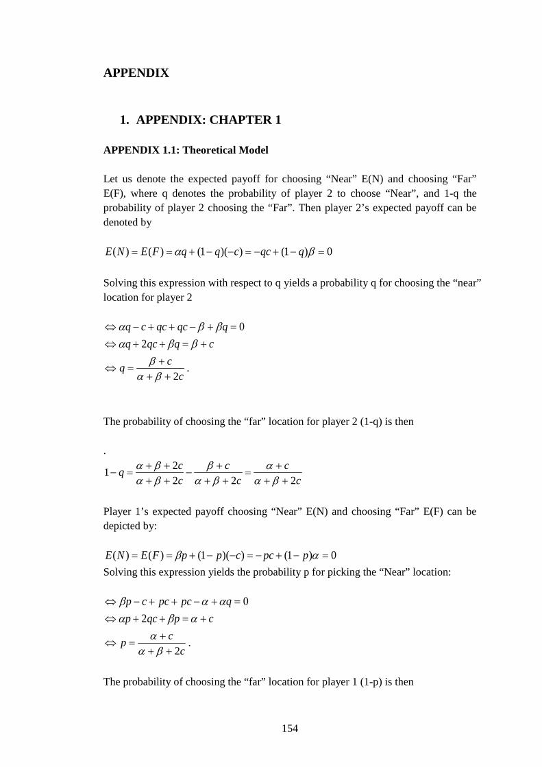
154
APPENDIX
1. APPENDIX: CHAPTER 1 APPENDIX 1.1: Theoretical Model Let us denote the expected payoff for choosing “Near” E(N) and choosing “Far” E(F), where q denotes the probability of player 2 to choose “Near”, and 1-q the probability of player 2 choosing the “Far”. Then player 2’s expected payoff can be denoted by
Solving this expression with respect to q yields a probability q for choosing the “near” location for player 2
.
The probability of choosing the “far” location for player 2 (1-q) is then .
Player 1’s expected payoff choosing “Near” E(N) and choosing “Far” E(F) can be depicted by:
Solving this expression yields the probability p for picking the “Near” location:
.
The probability of choosing the “far” location for player 1 (1-p) is then
0)1())(1()()( =−+−=−−+== βα qqccqqFENE
0=+−++−⇔ qqcqccq ββαcqqcq +=++⇔ ββα 2
ccq
2+++
=⇔βα
β
cc
cc
ccq
22221
+++
=++
+−
++++
=−βα
αβα
ββαβα
0)1())(1()()( =−+−=−−+== αβ ppccppFENE
0=+−++−⇔ qpcpccp ααβcpqcp +=++⇔ αβα 2
ccp
2+++
=⇔βα
α

155
So by symmetry:
and
The probability of a successful coordination P(S) thus is expressed as .
Simplifying this yields probability of successful coordination of
Where the Probability of coordination on both the Near and the Far equilibrium is:
Given that c > 0, all probabilities are strictly positive. Formally: looking at the partial derivative ∂P(S) with respect to c it becomes apparent that with an increasing c the probability of coordination strictly increases. The derivative can be depicted as
Applying the quotient rule the expression becomes
With further simplification the derivative becomes
cc
cc
ccp
22221
+++
=++
+−
++++
=−βα
ββα
αβαβα
ccpq
21
+++
=−=βα
β
ccqp
21
+++
=−=βα
α
cc
cc
cc
ccSP
2*
22*
2)(
+++
+++
+++
+++
+=
βαβ
βαα
βαβ
βαα
( )22))((2)(
cccSP
++++
=βα
βα
( )2, 2))((
2*
2)(
ccc
cc
ccSP FN ++
++=
+++
+++
=βαβα
βαβ
βαα
[ ]( )[ ]22
))((2)(c
cccSP
++∂++∂
=∂
∂βα
βα
[ ] ( ) ( )[ ]( )[ ]2
22
22*))((22*))((2
ccccccc
++∂++∂++−++++∂
⇔βα
βαβαβαβα

156
. Simplifying the terms
The function is decreasing in c, as c >=0, the function is decreasing as c increases. Looking at the effect of a change in c on the probabilities of coordinating on the near and far equilibria (as they are symmetric):
Applying the quotient rule the term becomes
Then through simplification we receive
The derivative thus is
The derivative of P´(SN,F) is strictly positive as the expressions in the numerator and denominator are always positive. Hence the probabilities for coordinating on the near and far equilibrium decrease in c as well.
( ) ( ) ( ))('
2))((8
2)(2
2)(2
322 SPc
ccc
cc
c=
++++
−+++
++++
⇔βα
βαβαβ
βαα
( ))('
2)(2
3
2
SPc
=++−
⇔βα
βα
[ ]( )[ ]2
,
2))(()(
ccc
cSP FN
++∂++∂
=∂
∂
βαβα
[ ] ( ) ( )[ ]( )[ ]2
22
22*))((2*))((
ccccccc
++∂++∂++−++++∂
⇔βα
βαβαβαβα
( ) ( ) ( ))('
2))((4
2)(
2)(
322 SPc
ccc
cc
c=
++++
−+++
++++
⇔βα
βαβαβ
βαα
( ))('
2)(2
3
2
SPc
=++−
⇔βα
βα

157
Pure win and loss frames
Adding or subtracting a factor to the expected payoff functions will keep the game theoretic prediction of the game equivalent. This makes it possible to create a pure win or pure loss frame. Regarding the expected payoff functions for player 1 and 2 subject to an external factor Δ:
Solving this expression with respect to q yields a probability q for choosing the “near” location for player 2 yields as before
.
The probability of choosing the “far” location for player 2 (1-q) is then
By symmetry this holds also for player 1
q.e.d.
0))(1()())(1()()()( =+∆−−−∆−−∆−++∆== βα qqccqqFENE
0=∆++−∆−+∆−+∆−−∆+∆+⇔ qqcqqqcqcqq ββαcqqcq +=++⇔ ββα 2
ccq
2+++
=⇔βα
β
ccq
21
+++
=−βα
α
ccpq
21
+++
=−=βα
β
ccpq
21
+++
==−βα
α
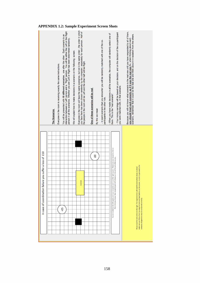
158
APPENDIX 1.2: Sample Experiment Screen Shots

159

160

161

162

163

164

165
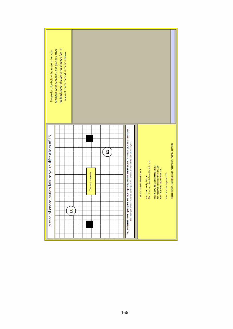
166

167
2. APPENDIX: CHAPTER 2
APPENDIX 2.1: Alternating Offers Bargaining Theory
The standard alternating offer bargaining model 19 with a shrinking pie
assumes two players, A and B, that engage in alternating offers over the division of a
pie π, π > 0. Player A makes the first offer on how to divide the cake, player B either
accepts or rejects the offer. If player B accepts then the game is over. If player B
rejects the offer, player B will make a an offer at a time Δ = 2. Should player A
reject the offer then player A will make anew an offer at time Δ = 3. The process
continues until an offer is accepted or until the amount to be distributed becomes 0.
An offer is a number between 0 and π. The payoffs of player i in this case are a share
of the pie π depicted by π≤≤ ix0 such that ( )∆− trx ii exp where ri > 0 is the
discount rate of player i. Time is discounted as 20 ( )∆−≡ ii rexpδ .
Two properties21 necessary for the equilibrium are that whenever a player has
to make an offer, and it is an equilibrium offer, it is accepted by the other player and
also in equilibrium a player makes the same offer whenever she has to make an offer
(Muthoo, 1999, pg.44). Given these properties the loss of player B rejecting an offer
from A will be *bbxδ , since after rejecting player B will offer the equilibrium share of
*bx . Hence, player B accepts any offer ax such that *
bba xx δπ >− . By the first
property mentioned above **bba xx δπ ≥− . However, if **
bba xx δπ >− , then player A
could increase her payoff with an alternative offer that is higher. Hence we have the
symmetric outcome of **bba xx δπ =− and **
aab xx δπ =− which leads to the
unique solution of πµaax =* and πµbbx =* , where ba
ba δδ
δµ−−
=11 and
ba
ab δδ
δµ−−
=11 22.
In a Subgame Perfect Equilibrium player A always offers *ax and accepts bx if
*aab xx δπ >− , thus player A always demands a share of
ba
b
δδδ
−−
11 while accepting no
19 The model as follows has been created by Rubinstein (1982). 20 As presented in (Muthoo, 1999, pg. 42) 21 Following: the Rubinstein alternate offer model as presented by Muthoo (1999). 22 The properties mentioned as well as the presentation of the model stems from (Muthoo, 1999, pg 44).
168
offer smaller then ( )ba
bb
δδδδ
−−
11 23. The proof of optimality of this distribution is given
considering that at any point in time ∆t player A makes an offer such that *a
ta xx ≤ .
In which case player B accepts immediately, so a deviation is not profitable
(Muthoo, 1999, pg.45). In case of *a
ta xx ≥ player B rejects any offer made. Hence *
ax
and *bx are equilibrium offers. The general idea of a sequential round alternating
offer bargaining game is that players accept an offer in each round that is at least as
high as the outcome they would get in the next round. Binmore et al. (2007) test the
robustness of the Rubinstein bargaining solution and find that the solution holds up
in experimental results24.
In case of a fixed amount being deducted from an amount to be distributed π,
players know the pie size in the next round Δ+1, where πΔ > π Δ+1 for 1 ≤ Δ ≤ 14.
Offers can be made in each round by players within the range of Ω Є 0, πΔ starting
with player A in round 1. If an agreement is reached players will earn ΩΔ for the
proposer and πΔ - ΩΔ for the responder. Following the reasoning above there is a
subgame perfect equilibrium in the sequential game using the on using the one step
diviation principle (Fudenberg & Tirole, 1991). Suppose in any given period Δ
player a offers player b the split of ΩΔa such that player B receives ΩΔa and player A
receives πΔ - ΩΔa if player B accepts. Player a knows that if b rejects in the next
round he will only obtain ΩΔb where player b would earn πΔ - 1 - ΩΔb. Now player A
knows that he has to offer at least ΩΔa ≥ πΔ - 1 - ΩΔb, otherwise player b will reject
the initial offer. If ΩΔa > πΔ - 1 - ΩΔb player a can improve by making a lower offer.
Player B knows this and needs to accept ΩΔa by player A. If player b rejects the
maximum he can get is πΔ - 1 - ΩΔb in the next round. Player a will not offer more
than πΔ - 1 - ΩΔb and accept no less than ΩΔb. Due to the fact that πΔ – 1 < πΔ and
Ω*Δb = πΔ - 1 - ΩΔb the only possible alternative for player B in period πΔ + 1 player
a will offer Ω*Δa = ΩΔa to player b and he accepts.
Looking at backward induction in the final round of the game (Δ = 14), if no
agreement has been reached before, the amount to be distributed drops to 0, and both
participants would thus receive 0. In round Δ = 13 the amount to be distributed is π13
23 cf. Fudenberg, 1991 24 Another option would have been to make offers retractable (Muthoo, 1995), however, the emphasis in this experiment was to observe first offers when offers are binding.

169
= 1. Player a can select from two possible distributions of the pie Ω13 = (1/0, 0/1).
Player A will in this case allocate 1 for himself and 0 to player b (1/0). Player B
accepts a payoff of 0 as he is indifferent to the payoffs in Δ = 13 and Δ = 14. In
round Δ = 12 the amount to be distributed is 2 and player B knows that the
maximum payoff for player A is 1 in round Δ = 13, thus offers him an amount that is
at least as high. Given an offer range of Ω12 = (0/2, 1/1, 2/0), player B offers player
A division of ½ / ½ of the pie so £ 1 each. This offer makes player A indifferent and
thus accept the offer of player B. Following that logic in round Δ = 12 player A
proposes a split that yields £ 2 and £ 1 for player B, as this is the maximum amount
he can obtain in the next round. Following the backward induction the initial offer of
player A is £ 7 for himself and £ 6 to player B and player B accepts.
APPENDIX 2.2: Ultimatum Game Bargaining Theory
Suppose two players engage in an Ultimatum Game to divide up a pie P.
Player A makes a proposal to keep amount Ω in the range of [0, P] and to give to
player B (P – Ω). Player B can then accept or reject the offer subject the function his
f(0, P), choosing which offer to accept and which to reject. If player B accepts player
A receives Ω and player B receives P – Ω. The strategy pair is thus (Ω, f(Ω)). The
subgame perfect Nash equilibrium of the game is reached if f(Ω) is accepted and if
there is no other offer θ , with θ > Ω where f(θ) = accept. Players do not increase their
demands, as they would get 0. Thus player A gives player B the minimum possible
amount and player B accepts (SPNE).

170
APPENDIX 2.3: Instructions

171

172

173

174

175

176

177

178

179

180

181

182

183

184

185

186
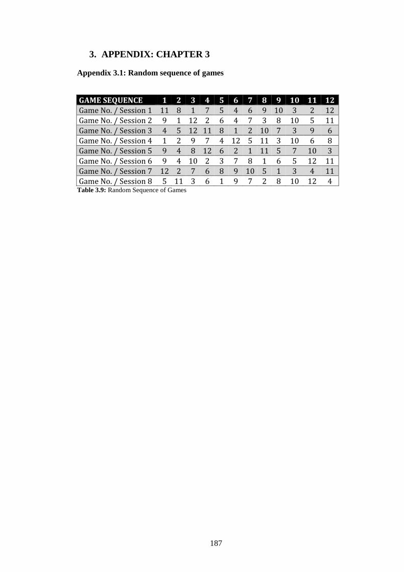
187
3. APPENDIX: CHAPTER 3
Appendix 3.1: Random sequence of games
GAME SEQUENCE 1 2 3 4 5 6 7 8 9 10 11 12 Game No. / Session 1 11 8 1 7 5 4 6 9 10 3 2 12 Game No. / Session 2 9 1 12 2 6 4 7 3 8 10 5 11 Game No. / Session 3 4 5 12 11 8 1 2 10 7 3 9 6 Game No. / Session 4 1 2 9 7 4 12 5 11 3 10 6 8 Game No. / Session 5 9 4 8 12 6 2 1 11 5 7 10 3 Game No. / Session 6 9 4 10 2 3 7 8 1 6 5 12 11 Game No. / Session 7 12 2 7 6 8 9 10 5 1 3 4 11 Game No. / Session 8 5 11 3 6 1 9 7 2 8 10 12 4
Table 3.9: Random Sequence of Games

188
Appendix 3.2: Instructions

189

190
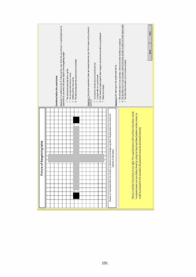
191

192
193

194

195

196

197

198

199
200