essays on bank transparency - universität mannheim
TRANSCRIPT

Essays on Financial Reporting Incentives
and Bank Transparency
Inauguraldissertation zur Erlangung des akademischen Grades
eines Doktors der Wirtschaftswissenschaften der Universität
Mannheim
vorgelegt von
Nicolas Rudolf
Stuttgart

ii
Dekan: Prof. Dr. Christian Becker
Referent: Prof. Dr. Jannis Bischof
Korreferent: Prof. Dr. Holger Daske
Tag der mündlichen Prüfung: 2. Juli 2020

iii
Table of Contents
List of Figures v
List of Tables vi
Nomenclature vii
Introduction 1
Chapter 1
1.1. Introduction 10
1.2. Prior research and empirical predictions 15
1.2.1. Empirical approaches to identify manager characteristics 15
1.2.2. The role of individual managers in banks’ loan loss provisioning choices 17
1.2.3. The role of top management team composition 19
1.3. Data 20
1.4. Measuring loan loss provisioning quality 21
1.5. The role of individual managers in the LLP choice 22
1.5.1. Research design 22
1.5.2. Results 30
1.6. Management styles and the LLP choice 39
1.6.1. Research design 39
1.6.2. Results 43
1.7. Interaction with team composition 52
1.7.1. Research design 52
1.7.2. Results 53
1.8. Conclusion 55
1.9. Appendix A: Variable definitions 57
Chapter 2
2.1. Introduction 58
2.2. Institutional setting and empirical predictions 64
2.2.1. Bank supervision and enforcement under the Single Supervisory Mechanism 64
2.2.2. Banks’ reporting behavior around the supervisory AQR disclosures 67
2.2.3. Bank transparency around the supervisory AQR disclosures 69
2.3. Research design and data 69
2.3.1. Empirical model 69
2.3.2. Sample selection and descriptive statistics 73

iv
2.4. Empirical results 81
2.4.1. Changes in financial reporting following SSM adoption 81
2.4.2. Changes in liquidity following SSM adoption 84
2.4.3. Cross-sectional heterogeneity: enforcement and market monitoring 86
2.4.4. Timeliness of the loan loss provision 96
2.5. Conclusion 99
2.6. Appendix B: Variable definitions 102
2.7. Appendix C: Entropy balancing 103
Chapter 3
3.1. Introduction 104
3.2. Literature review 109
3.3. Research design and data 111
3.4. Empirical results 115
3.4.1. Descriptive statistics 115
3.4.2. What determines the duration of NPL cycles? 119
3.4.3. Country-level versus bank-specific determinants of NPLs 121
3.4.4. The role of contract enforcement and insolvency proceedings for NPLs 124
3.4.5. Robustness tests 126
3.5. Conclusion 129
3.6. Appendix D: Variable definitions 130
Concluding Remarks 132
References 134
Curriculum Vitae 148

v
List of Figures
Figure 2.1 Accounting effects around SSM introduction and AQR disclosures 77
Figure 3.1 NPL ratios and GDP development for high vs. low legal efficiency countries 115
Figure 3.2 GDP development for high vs. low legal efficiency countries 116

vi
List of Tables
Table 1.1 Manager mobility and connectedness 26
Table 1.2 Summary statistics and sample representativeness 28
Table 1.3 Manager attributes, controls, fixed effects and the adjusted R² 31
Table 1.4 Statistical and economic importance of manager fixed effects 33
Table 1.5 Robustness tests: economic significance of manager fixed effects 37
Table 1.6 Correlation across management styles and individual characteristics 44
Table 1.7 Cross-sectional variation of manager fixed effects 49
Table 1.8 Manager profiles 51
Table 1.9 Top management team composition and bank outcomes 54
Table 2.1 Sample selection 74
Table 2.2 Descriptive statistics 79
Table 2.3 Loan loss reporting following SSM introduction and AQR disclosures 83
Table 2.4 Liquidity effects following SSM introduction and AQR disclosures 85
Table 2.5 Cross-sectional variation in accounting and liquidity effects 91
Table 2.6 Timeliness of loan loss provisions 98
Table 3.1 Descriptive statistics and pairwise correlations on the country level 118
Table 3.2 Influence of legal efficiency and GDP on the duration of NPL cycles 120
Table 3.3 Descriptive statistics on the bank level 122
Table 3.4 Legal efficiency along the economic cycles and NPL ratios 123
Table 3.5 Contract enforcement, insolvency procedures and NPL ratios 125
Table 3.6 Robustness tests with additional controls 128

vii
Nomenclature
AQR Asset Quality Review
CEO Chief Executive Officer
CFO Chief Financial Officer
CIO Chief Information Officer
CRO Chief Risk Officer
CPA Certified Public Accountant
ECB European Central Bank
GDP Gross Domestic Product
IMF International Monetary Fund
LLP Loan Loss Provision
NBER National Bureau of Economic Research
NPL Non-Performing Loan
OLS Ordinary Least Squares
PCA Principle Component Analysis
SSM Single Supervisor Mechanism

1
Introduction
The global financial crisis placed bank transparency in the limelight of public interest
(Financial Times, 2010). A major source of bank transparency is banks’ financial reporting that
helps to inform depositors, regulators, supervisors, and capital market participants about banks’
financial position, performance, business activities, and in particular risk-taking (Bushman and
Williams, 2015; Freixas and Laux, 2012). 1 However, accounting information from financial
statements is only a noisy representation of the underlying economic reality as the rules that govern
the reported numbers often require the exercise of judgement (Bushman, 2016).
The discretion inherent to accounting standards has two faces (Kanagaretnam, Lobo and
Yang, 2004). On the one hand, accounting discretion can increase transparency by allowing
managers to convey private information to outsiders when having superior knowledge about a
transaction that can otherwise not be reflected in the accounting system (e.g., Beaver, Eger, Ryan
and Wolfson, 1989; Wahlen, 1994). On the other hand, managerial discretion can also lead to the
opportunistic application of accounting rules driven by reporting incentives that, in turn, undermine
bank transparency (e.g., Vyas, 2011; Bischof, Laux, and Leuz, 2020).
One major accounting choice in the banking industry that involves substantial managerial
discretion is the accounting for loan losses (Liu and Ryan, 2006; Barth and Landsman, 2010; Beatty
and Liao, 2014; Gebhard and Novotny-Farkas, 2011). Loans are economically important for banks
as they are the largest asset on most banks’ balance sheets and loan loss provisions represent the
largest bank accrual for the majority of banks (Beatty and Liao, 2014; Acharya and Ryan, 2015).
1 Bank transparency has many facets and ultimately arises from information collection, verification, and
dissemination to stakeholders outside the bank who utilize this information in their decision making (Bushman,
2014; Freixas and Laux, 2012).

2
During and after the global financial crisis (2007-2008) the accounting rules for loan loss
provisions were frequently blamed for encouraging banks to recognize delayed and insufficient
provisions as cushions against future loan losses (Dugan, 2009; Curry, 2013).2 This critique
ultimately resulted in the introduction of redesigned and more forward-looking provisioning
standards in Europe (IFRS 9) and the United States (ASU 2016-13).
However, banks’ reporting choices can be influenced by a variety of incentives and
pressures that go far beyond the design of accounting standards per se (Beatty and Liao, 2014;
Bushman, 2014). Bank-specific incentives such as capital market pressure, private ownership,
taxation, or regulation are associated with discretion in recognizing loan losses (e.g., Beatty et al.,
1995, 2002; Collins et al., 1995; Ahmed et al., 1999; Bushman and Williams, 2012). Furthermore,
individual manager incentives and preferences that are correlated with risk-taking, capital structure,
and corporate reporting choices in general could play a significant role for banks’ provisioning
behavior (Armstrong et al., 2010; Bamber et al., 2010; Bertrand and Schoar, 2003; Ge et al., 2011).
Besides the discretion that arises from accounting standards or individual manager
preferences, the institutional design and in particular enforcement can influence firms’ reporting
behavior (Christensen, Hail, and Leuz, 2013; Holthausen, 2009). In the banking sector, dedicated
bank supervisors tend to dominate the public enforcement of reporting regulation (Bischof, Daske,
Elfers, and Hail, 2020). However, the supervisory and regulatory toolkit is not limited to direct
enforcement by intervention into banks’ business activities through penalties and other corrective
actions. Bank supervisors can also take alternative actions to influence bank behavior such as
2 The adverse consequences of delaying loan loss provisioning are manifold, feedback to the real economy and
impair financial stability (Bushman and Williams, 2016; Ahmed, Takeda, and Thomas, 1999; Beatty and Liao,
2011).

3
disclosures about banks’ risk exposure (e.g., through stress tests) in order to promote market
discipline that eventually inhibits excessive risk-taking and fosters transparency (Goldstein and
Sapra, 2014; Goldstein and Yang, 2019; Bischof and Daske, 2013).
This thesis consists out of three chapters that all add to the literature on bank transparency.
While the first chapter explores determinants of bank transparency at the most granular level by
looking at individual managers and how they shape financial reporting decisions, the second and
the third chapter document the role of bank, country, and supranational reporting incentives for
banks’ reporting choices. Within the next paragraphs, I describe the chapters of my thesis in more
detail.
In Chapter 1, I start with an investigation of individual managers and their inherent
characteristics as potential determinants of banks’ financial reporting decisions. The first chapter
is based on a working paper that I wrote together with Jannis Bischof (University of Mannheim)
entitled “Manager Characteristics and Banks’ Loan Loss Provisioning”. While prior literature
provides ample evidence on a variety of incentives and pressures that explain the variation in
provisioning behavior across banks and over time, we know much less about variation in
provisioning behavior within banks (Beatty and Liao, 2014; Bushman, 2014). Because the
incentives and preferences of individual managers are associated with corporate reporting choices
in general (Armstrong et al., 2010; Bamber et al., 2010; Ge et al., 2011), it is highly plausible that
the characteristics of individual managers also play a role in a bank’s loan loss provisioning. A
better understanding of this role is particularly important because recent regulation in the banking
sector is targeting the qualifications of individual managers (e.g., ECB, 2018a). These regulations
can only be effective if individual managers’ actions are meaningfully correlated with reporting
choices that affect bank transparency such as the loan loss provisioning behavior.

4
We build on research in finance (Malmendier et al., 2011; Nguyen et al., 2017) and
accounting (Ahmed et al., 2019; Livne et al., 2011; Bushman et al., 2018) that documents the
influence of manager characteristics on corporate policies and examine whether idiosyncratic
management styles help explain banks’ loan loss provisioning choices. In contrast to prior
literature that primarily focuses on specific traits and incentives, we identify the impact of
unobservable traits that in combination translate into individual management styles. We first
disentangle and quantify this individual manager influence from firm-specific factors.
Furthermore, we explore how individual management styles interact with top management team
composition.
To analyze the role of manager styles, we build on a dataset of top managers of US banks
over the period from 1993 to 2015. We combine information from different datasets that include
observable characteristics (e.g., compensation, education, experience), firm characteristics (e.g.,
size, risk, performance), and accounting choices. In a first step of our analysis, we test for the
association between discretionary loan loss provisions and manager characteristics. In our analysis,
we distinguish between observable and unobservable characteristics. We capture unobservable
characteristics through a three-way fixed-effects structure that exploits the interconnectedness
between managers that switch to another sample bank and managers that remain at the same bank
(Abowd et al., 1999; hereafter AKM method). These fixed effects capture all time-invariant
manager characteristics and can be described as management styles for observable management
choices even if the underlying factors explaining these choices remain unobservable. Our results
suggest that observable manager characteristics explain only a small amount of the variation in
banks’ discretionary loan loss provisions, whereas idiosyncratic, yet unobservable attributes of
individual managers account for approximately 19% of this variation (compared to 12% for

5
unobservable firm attributes). This finding does not imply that individual bank managers have
little influence on accounting choices, but rather that managers exert this influence through their
preferences, skills, or talent that are notoriously hard to measure but key to a full understanding of
managers’ role in the accounting process.
In the second step, we explore whether managers loan loss provisioning styles relate to
other relevant corporate actions. We document a systematic correlation between the loan loss
provisioning style and management styles for various corporate policies. For example, managers
with a greater level of discretion in the loan loss provisioning choice also reveal a preference for a
higher level of risk-taking and, on average, a lower quality of the loan portfolio. That is, managers
loan loss provisioning styles are systematically related to other corporate actions.
In the third and final step, we build on the classification by Pitcher and Smith (2001) and
distinguish between four different types of managers: technocrats, artists, craftsmen, and
traditionalists. Our classification rests on the manager styles that we identified through the AKM
method in the previous step. We use the different manager styles of members of a bank’s top
management to get a measure for the diversity of top management teams that is derived from
observable preferences for specific corporate actions. Based on these measures, we analyze
whether the composition of top management teams potentially mutes the role that idiosyncratic
manager styles play in the loan loss provisioning choice. We show that diversity of manager styles
in the top management team mutes the significant association between the individual manager style
and the level of reporting discretion.
In Chapter 2, which is based on a working paper that I wrote together with Jannis Bischof
(University of Mannheim) and Ferdinand Elfers (Erasmus School of Economics) entitled “Do

6
Supervisory Disclosures Lead to Greater Bank Transparency? The Role of Enforcement and
Market Discipline”, we empirically investigate how bank supervisors can influence the
transparency of supervised firms through enforcement and supervisory disclosures.
In this project, we explore how a plausibly exogenous change in enforcement in conjunction
with the supervisory disclosure of banks’ asset quality affects bank transparency. We exploit the
shift from a purely national banking supervision to a unified European supervisor to identify
differences in supervisory reporting preferences. Since it is not straightforward to determine an
objective and comparable measure of supervisory reporting preferences, we exploit the
simultaneous Asset Quality Review (AQR) disclosures by the ECB. This assessment included a
point-in-time assessment of the accuracy of the carrying values of banks’ assets with a particular
focus on the classification of non-performing exposures and loan loss provisions. However, most
of the AQR adjustments were not reflecting violations of accounting rules, but rather signaled a
shift in supervisory reporting preferences within a common accounting framework, with the ECB
generally preferring higher levels of provisioning than the national supervisors previously in charge
of bank supervision. We exploit this firm-level variation as well as the staggered shift to ECB
supervision to analyze the change in affected banks’ reporting behavior and transparency in a
difference-in-difference framework.
We find that the ECB’s disclosed reporting preference is reflected in banks reporting
behavior and market liquidity in the following periods. We interpret this as evidence that banks’
reporting choices are influenced by supervisory preferences beyond simple compliance with given
accounting standards. The effect on banks reporting behavior is particularly pronounced for banks
that experienced the greatest shift in supervisory characteristics. That is, banks whose prior national
supervisory environment was characterized by low supervisory quality or had a higher likelihood

7
of political capture before the SSM. We observe a corresponding effect on market liquidity that is
more pronounced for banks that are likely to be subject to market discipline. Furthermore, we
identify the timeliness of loan loss provisions as potential channel through which the shift in
reporting translates into reduced information asymmetry. Overall, our findings suggest that
supervisory disclosures are potentially effective in establishing greater transparency of the banking
sector, but depend on the presence of firm-level incentives that help to establish market discipline.
In Chapter 3, which is based on a working paper with the title “Legal Efficiency and Non-
Performing Loans along the Economic Cycle”, I study how cross-country differences in legal
efficiency interact with non-performing loans along the business cycle. Many banks faced elevated
levels of NPLs after the global financial crisis and the sovereign debt crisis. However, NPLs still
represent a burden for banks balance sheets with European banks holding more than 580 billion
euros of non-performing exposures at the end of March 2019 (ECB, 2019). I start this study from
the observation that in the aftermath of the severe economic downturn in the Eurozone caused by
the global financial crisis and the sovereign debt crisis, only a subset of countries was able to
substantially decrease their NPLs although most countries were facing favorable economic
conditions .
One explanation for this phenomenon could be the severe differences in contract
enforcement and insolvency regimes across Europe that exacerbate uncertainty for banks and lead
to slow loan write-offs. Banks often have to wait for courts deciding on cases in order to determine
the amount that has to be written off. A typical foreclosure process (for a mortgage loan) in
northern Europe can take up to three years, while it can be up to eight years in Greece (Fitch, 2016).
However, despite the high importance of a swift process to resolve non-performing loans, there is

8
a lack of research on the impact of bank-specific or institutional determinants such as legal
efficiency that potentially influence the duration of the NPL cycle.
In the first step, I employ a proportional hazard model on the country-level to answer the
question whether legal efficiency and economic growth influence the duration of NPL cycles. I
document that the increasing NPL phase is mainly associated with macroeconomic factors such as
economic growth. However, the duration until a bank can decrease its NPL levels after the country
enters an economic growth phase is substantially shorter for banks in countries with higher legal
efficiency. In the second step, I employ bank-level data to compare how macroeconomic, bank-
specific factors and institutional differences in legal efficiency are associated with NPLs over the
economic cycle. I employ various proxies for legal efficiency from prior literature (Djankov La
Porta, Lopez-de-Silanes and Shleifer, 2003; Djankov, Hart, McLiesh, and Shleifer, 2008). My
results consistently document that the duration and costs of contract enforcement and insolvency
procedures are negatively associated with NPL ratios during economic growth phases. Taken
together my analyses documents that legal efficiency is significantly associated with NPL
resolution whereas the increasing NPL phase is mainly determined by economic growth.
This thesis provides answers to three important research questions related to financial
reporting incentives and bank transparency. In Chapter 1, I document that a large proportion of the
variation in banks loan loss provisioning behavior is explained by individual bank manager
characteristics. Furthermore, the research presented in Chapter 2 documents that supervisory
disclosures can foster market discipline that lead to higher overall bank transparency. Finally, in
Chapter 3, I provide evidence on the association between legal efficiency and non-performing loans
along the business cycle that can help to inform the regulatory and supervisory debate on measures

9
to deal with elevated NPL levels that are likely to emerge after the recent virus-related economic
downturn in many countries.

10
Chapter 1
Manager Characteristics and Banks’ Loan Loss Provisioning
1.1. Introduction
What determines banks’ loan loss provisioning choices? Prior literature provides ample
evidence on a variety of incentives and pressures that explain the variation in provisioning behavior
across banks and over time (Beatty and Liao, 2014; Bushman, 2014). However, we know much
less about variation in provisioning behavior within banks (Bushman and Williams, 2015).
Individual managers shape corporate actions such as risk-taking and capital structure choices
(Bertrand and Schoar, 2003; Graham, Harvey & Puri, 2013). Their incentives and preferences are
associated with corporate reporting choices in general (Armstrong et al., 2010; Bamber et al., 2010;
Ge et al., 2011). However, little evidence exists on management’s role in the timing of loan loss
recognition (Beatty and Liao, 2014). A better understanding of this role is especially important
because recent regulation in the banking sector is targeting the qualifications of individual
managers (e.g., ECB, 2018a). The potential impact of these regulations hinges on the influence
that individual managers actually have on critical actions such as the loan loss provisioning choice.
Against this background, we build on research in finance (Malmendier et al., 2011; Nguyen
et al., 2017) and accounting (Ahmed et al., 2019; Livne et al., 2011; Bushman et al., 2018) that
investigates the influence of manager characteristics on corporate policies and examine whether
idiosyncratic management styles help explain banks’ loan loss provisioning choices. In contrast to
prior literature that primarily focuses on specific traits and incentives, we identify the impact of

11
unobservable attributes that, in combination, translate into an individual management style. We
disentangle the overall influence of these idiosyncratic styles on the reporting outcome from firm-
specific factors. In addition, we analyze how these management styles interact with top
management team composition.
To address these questions, we construct a comprehensive dataset of top executives of US
banks over the period from 1993 to 2015. The dataset combines information about manager
characteristics (e.g., compensation, education, experience), firm characteristics (e.g., size, risk,
performance), and accounting choices. In a first step of our analysis, we test for the association
between discretionary loan loss provisions and manager characteristics. We distinguish between
observable and unobservable characteristics. We capture unobservable characteristics through a
fixed-effects structure that exploits the interconnectedness between managers that switch to another
sample bank and managers that remain at the same bank (Abowd et al., 1999; hereafter AKM
method). These fixed effects are supposed to capture latent time-invariant manager styles that
describe preferences for observable management choices even if the underlying factors explaining
these choices remain unobservable.
In a second step, we analyze how the role of idiosyncratic manager styles in the choice of
loan-loss provisions relates to other relevant corporate actions. To this end, we compare the time-
invariant manager style that manifests in the choice of loan loss provisions with other management
choices that affect a bank’s risk-taking (such as leverage or loan quality). To better understand
commonalities in the role that individual managers play in these different decisions, we test
whether these fixed effects (i.e., the different manager styles) are associated with observable
demographics, occupational status, or education of individual managers and with their risk-taking
incentives. Put differently, we test whether the unobservable style that the fixed-effects capture

12
under the AKM method is systematically correlated with observable factors. We follow
Baik et al. (2011) and also employ principal components analysis to combine these different factors
and construct a manager-specific score to overcome the noise inherent to the measurement of
individual characteristics and incentives.
In a third and final step, we build on the classification by Pitcher and Smith (2001) and
distinguish between four different types of managers: technocrats, artists, craftsmen, and
traditionalists. Our classification rests on the manager styles that we identified through the AKM
method. We use the different manager styles of members of a bank’s top management to get a
measure for the diversity of top management teams that is derived from observable preferences for
specific corporate actions. Based on these measures, we analyze whether the composition of top
management teams potentially mutes the role that idiosyncratic manager styles play in the loan loss
provisioning choice.
Our results suggest that observable manager characteristics and incentives explain only a
relatively small amount of the variation in banks’ discretionary loan loss provisions. We rather
find that idiosyncratic, yet unobservable attributes of individual managers account for
approximately 19% of this variation (compared to 12% for unobservable firm attributes). The low
correlations between observable characteristics and reporting outcomes thus do not imply that
individual bank managers have little influence on accounting choices. Managers exert this
influence in an idiosyncratic way through their preferences, skills, or talent that are notoriously
hard to measure but key to a full understanding of managers’ role in the accounting process.
We find that some observable characteristics are correlated with the unobservable factors
that reflect preferences for observable outcomes at the firm level. However, these correlations are

13
little systematic and they vary substantially across different corporate policies that managers
potentially influence. Most of the cross-sectional variation in manager styles remains, therefore,
unexplained. The manager styles are still economically meaningful because the direction of the
underlying preferences for certain corporate policies appears systematic. For example, managers
with a greater level of discretion in the loan loss provisioning choice also reveal a preference for a
higher level of risk-taking and, on average, a lower quality of the loan portfolio. That is, managers
who have a distinct impact on the loan loss provisioning do exert their influence on other corporate
actions in a systematically related way. We exploit these relations to construct four different
categories of managers that we label according to Pitcher and Smith (2001). Managers whom we
label as ‘technocrats’ and ‘artists’ employ systematically more discretion in the provisioning choice
than ‘craftsmen’ and ‘traditionalists’. These associations are statistically significant and
economically meaningful.
However, we also find evidence consistent with these top managers interacting with other
members of the executive board. Diversity of manager styles in the top management team mutes
the significant association between the individual manager style and the level of reporting
discretion. Overall, these findings suggest that the focus of bank supervisors on the skills and
qualifications of individual managers can be justified by the systematic impact that these
characteristics have on relevant corporate policies, at least in combination with other members of
the top management team. Yet, the evidence also implies that the focus should build on top
managers’ revealed preferences as reflected in key policies rather than on readily observable
attributes.
Our study contributes to two different streams of the accounting literature. First, we add to
the understanding of the determinants of banks’ loan loss provisions. Going back to at least Beaver

14
et al. (1989), the literature on the discretion and timing in recognizing loan losses has examined
various bank-specific incentives such as capital market pressure, private ownership, taxation, or
regulation (e.g., Beatty et al., 1995, 2002; Collins et al., 1995; Ahmed et al., 1999; Bushman and
Williams, 2012) as well as variation over time (e.g., Liu and Ryan, 2006; Beck and Narayanmoorth,
2013). However, we know relatively little about the impact of individual bank managers on the
provisioning choice. One recent exception is Ahmed et al. (2019) who document the association
between managers’ previous crisis experience and the timeliness of loan loss provisions during the
financial crisis. We extend this result beyond a single attribute and show the influence of both
observable and unobservable manager characteristics in crisis and non-crisis periods. This finding
helps understand the impact of recent regulation that targets the qualifications and behavior of
individual bank managers.
Second, we add to the growing literature on the impact of manager characteristics on
reporting outcomes in general. This literature documents that manager styles help explain
voluntary disclosure (Bamber et al., 2010), accounting choices (Ge et al., 2011; Dejong and Ling,
2013), disclosure tone (Davis et al., 2015), or tax avoidance (Dyreng et al., 2010). The role of
individual managers in the reporting process is associated with individual attributes such as military
experience (Law and Mills, 2017), masculinity (Jia et al., 2014), narcissism (Ham et al., 2018;
Young et al., 2016), religiosity (Dyreng et al., 2012), materialism (Bushman et al., 2018), gambling
attitudes (Christensen et al., 2018), tenure (Ali and Zhang, 2015), gender (Francis et al., 2015), age
(Huang, Rose-Green & Lee, 2012), ability (Demerjian et al., 2013), and overconfidence (Hribar
and Yang, 2016; Schrand and Zechman, 2012). The identification of individual attributes in these
prior studies typically relies on samples of managers who moved between firms and, therefore,
tend to have unique characteristics. We borrow from the literature in finance and economics (e.g.,

15
Graham, Li and Qiu, 2012; Lopes de Melo, 2018) and use the AKM method to expand the sample.
By exploiting the interconnectedness between moving and non-moving managers, we show that
the inclusion of non-moving managers into the sample substantially increases the explanatory
power of the manager characteristics. Related to this, we pick up recent insights on the importance
of board composition (e.g., Li and Wahid, 2018; van Peteghem, Bruynseels & Gaeremynck, 2018)
and present results consistent with the diversity of manager styles in a bank’s top management
muting the dominant influence of individual managers.
1.2. Prior research and empirical predictions
1.2.1. Empirical approaches to identify manager characteristics
Classic economic theory offers ambiguous predictions on whether the individual
characteristics of managers have any influence on corporate decisions. Neoclassical theory views
managers as homogeneous input into firms’ production process and variation in executive
characteristics do not play any role (Veblen, 1900; Bertrand and Schoar, 2003). Relatedly, the new
institutional theory suggests that organizational boundaries, conventions, and norms constrain the
impact of any individual on firm-level outcomes (e.g., DiMaggio and Powell, 1983).
In contrast to these predictions, Hambrick and Mason (1984)’s upper echelon theory builds
on managers’ personality, experience, and values being the main driver of organizational decisions
within a firm. Put differently, the upper echelons theory suggests that two seemingly identical
managers with a similar education, age, tenure, and compensation can vary in how they affect
corporate actions because of their latent unobservable personality and ability. While the recent
economic theory from Dessein and Santos (forthcoming) is consistent with these individual

16
manager effects, it attributes the idiosyncratic manager styles to attention allocation rather than to
cognitive biases of managers. Therefore, idiosyncratic manager effects could appear even when
manager’s information processing is optimal and not driven by behavioral biases.
Prior empirical literature offers evidence consistent with the upper echelons theory and the
attention theory by Dessein and Santos (forthcoming). These studies differ in the empirical
identification of the role of individual managers. A first set of studies focuses on a single
managerial trait and investigates, for example, the association between firm policies and manager-
specific variables such as gender (Francis et al., 2015), age (Huang et al., 2012), tenure (Ali and
Zhang, 2015), masculinity (Jia et al., 2014), ability (Demerjian et al., 2013), cultural heritage
(Brochet et al., 2019), and prior legal infractions (Davidson et al., 2015). While these studies
provide relatively robust evidence on the existence of these associations, individual managerial
traits likely manifest themselves not in isolation, but rather in certain combinations of specific
attributes (e.g., Adams et al., 2018). The empirical design of these studies does, by construction,
not disentangle the impact of the specific trait from other time-invariant firm attributes.
A second stream of literature exploits managerial mobility between firms to overcome the
inherent identification challenges. The use of mover-dummy variables isolates the manager styles
innate to managers that move between different firms. These manager styles capture bundles of
latent individual traits rather than specific characteristics. Evidence suggests that they are, inter
alia, associated with firms’ forecasting behavior (Bamber et al., 2010), conference call tone (Davis
et al., 2015), corporate tax avoidance (Dyreng et al., 2010), and earnings management (Ge et al.,
2011). However, the sample selection in the first place is confined to managers who move between
firms. If moving managers differ systematically from managers without any observable mobility,
the sample restriction leads to biased estimates because of endogenous matching between managers

17
and firms (Fee et al., 2013; Pan, 2017). For example, firms plausibly decide to replace managers
concurrently with the decision about certain policy changes, and therefore, any changes in
management style can overlap with the economic circumstances that caused the managerial
turnover in the first place.
The third and most recent approach is the employment of the AKM sampling technique.
The method accounts for the potential difference between moving and non-moving managers and,
therefore, does not solely rely on moving managers. Instead, the AKM method exploits the
connectedness between different groups of managers. Evidence that is derived from the application
of the AKM method suggests that individual manager styles affect compensation
(Graham et al., 2012), corporate social responsibility (Davidson et al., 2019), earnings
management (Wells, 2020), audit fees (Lauck et al., 2020), and tax avoidance (Law and Mills,
2017). We extend this stream of literature and employ the AKM method to explore the role of
individual bank managers in banks’ loan loss provisioning choices. To alleviate remaining
matching concerns, we additionally exploit a sub-sample of plausibly exogenous manager
turnovers.
1.2.2. The role of individual managers in banks’ loan loss provisioning choices
Banking is a highly regulated industry with regulation imposing relatively strong
constraints on the individual manager (e.g., Beatty and Liao, 2014; Hollander and Verriest, 2016).
For example, recent regulation (e.g., on management compensation) is increasingly limiting the
influence of individual manager’s incentives on bank-level decisions. At the same time, banking
supervisors become more involved in the screening of individual manager characteristics during
the recruiting process (e.g., Busch and Teubner, 2019). Against this background, the level of

18
management discretion in banks is relatively more confined than in other industries. For these low-
discretionary industries, the upper echelons theory and the attention theory predicts a lower
influence of idiosyncratic manager preferences on corporate decisions (Hambrick, 2007; Crossland
and Hambrick, 2007; Hambrick and Quigley, 2014; Dessein and Santos, forthcoming). Instead,
firm-level discretion mainly arises from environmental conditions and governance structures in
these types of industries.
On the other hand, in any regulated industry, it is unlikely that shareholders, boards, and
supervisors will be able to write perfect contracts that entirely limit discretion. This is particularly
critical for a task that is as inherently subjective and complex as the provisioning for future loan
losses. Banks have to recognize loan loss provisions if it is probable that a loan is impaired and if
the amount can be reasonably estimated. When bank managers assess these criteria, they frequently
distinguish between general loan loss provisions for portfolios of homogenous loans (e.g., different
classes of consumer loans) and specific provisions for large individual loans. They use complex
statistical models for the estimation of general loan loss provisions with the input into these models
being subject to substantial managerial judgment. The judgment is even greater when managers
determine individual loan loss provisions for large commercial loans and, through these decisions,
bank managers directly intervene into the corporate reporting choice. For these complex and
subjective tasks, the upper echelons theory predicts an even increasing impact of individual
characteristics and past experiences on corporate decision-making.
Overall then, the nature of regulation in the banking industry as well as the nature of the
loan loss provisioning task result in opposite predictions leaving the role of individual managers in
the shaping of banks’ loan loss provisioning behavior as, ultimately, an empirical question.

19
1.2.3. The role of top management team composition
While recent empirical evidence tends to support the notion of individual managers being
key to the explanation of corporate decisions, the literature also suggests that top management team
diversity mitigates this impact (Adams and Ferreira, 2010; Garlappi, Giammarino and Lazrak,
2017). That is, group dynamics can influence organizational outcomes even without the presence
of observable agency conflicts or information asymmetries. Prior evidence from non-banks
exploits differences along observable characteristics such as age, tenure or education and is
generally consistent with diversity also interacting with the managerial influence on corporate
reporting choices (e.g., Li and Wahid, 2018, Van Peteghem et al., 2018).
It is less clear whether these dynamics also evolve in banks’ loan loss provisioning
decisions. The decisions about general and individual loan loss provisions depend on highly
specific knowledge of individual managers. Educational and functional diversity is particularly
pronounced for board members in the banking industry and potentially leads to substantial
knowledge gaps (e.g., Berger et al., 2014; Macey and O’Hara, 2016). The difference in task
knowledge eventually translates into the reliance on one individual manager. This is consistent
with Graham et al. (2013)’s observations which suggest that oversight should “[...] use outsourced
expertise in technical subjects such as valuing assets like mortgage-backed securities, residual
assets or compliance with loan loss reserves” (p. 29).
There is very limited evidence on top management team diversity within banks. Extant
literature documents that educational and functional heterogeneity can prove beneficial for bank
innovations (Bantel and Jackson, 1989) and, especially, during mergers (Hagendorff,
Collins & Keasy, 2010). We build on this literature and investigate whether the diversity of top

20
management teams in banks moderates the influence of individual managers’ discretion on loan
loss provisions.
1.3. Data
We collect banks’ financial accounting data from Compustat banks, stock market data from
(CRSP) and manager data from ExecuComp3 and BoardEx. Our sample period spans from 1993
to 2014 because of data requirements about future and prior non-performing loans. We
identify 207 banks, 1,858 managers (9,893 observations) with available CRSP, Compustat,
BoardEx, and ExecuComp data. We limit the dataset to 108 banks that employed at least one
manager who switched to another bank during the sample period allowing us to separate firm and
manager effect with the AKM sampling technique. That is, our final dataset with available
information on manager characteristics from BoardEx and Execucomp includes 4,740 observations
and 911 distinct managers that worked for 108 banks.4 We focus on the five highest-paid managers
within each bank, including positions such as CEO, CFO, CRO (Chief Risk Officer), CIO (Chief
Information Officer), and General Counsel. While evidence from other industries suggests that
CEOs and CFOs differ in their influence over reporting decisions (Jiang et al., 2010), it is ex ante
unclear whether the idiosyncratic influence of bank managers on loan loss provisions is associated
with a specific job title within the top management team.
3 ExecuComp covers all banks that were included in the S&P 1500 at least for one year. ExecuComp is available for
periods from 1992 onwards. 4 That is, we capture roughly 50% of the full Execucomp-Boardex-Compustat sample, whereas the mover dummy
variable method (e.g. Betrand and Schoar, 2003; Bamber et al., 2010) would restrict the sample to 98 managers
that moved across banks (less than 11% of all managers in the full sample).

21
1.4. Measuring loan loss provisioning quality
For our investigation of manager’s loan loss provisioning choice, we follow Beatty and
Liao (2014) and measure banks loan loss provisioning quality by estimating a model that separates
the loan loss provision in a systemic and a discretionary part using quarterly bank data from
Compustat banks. If managers idiosyncratically influence the loan loss provision this should be
reflected in the variation of the loan loss provision that is not explained by macroeconomic and
firm fundamentals, such as changes in GDP or non-performing loans. Therefore, we use the
residuals from the following pooled OLS regression that capture only variation unaccounted for by
bank or macroeconomic fundamentals: 5
(1) 𝐿𝐿𝑃𝑗,𝑡 = 𝛼0+𝛽1∆𝑁𝑃𝐿𝑗,𝑡+1 + 𝛽2∆𝑁𝑃𝐿𝑗,𝑡+𝛽3∆𝑁𝑃𝐿𝑗,𝑡−1 + 𝛽4∆𝑁𝑃𝐿𝑗,𝑡−2+𝛽5∆𝐿𝑜𝑎𝑛𝑗,𝑡
+ 𝛽6𝑅𝑒𝑔𝑢𝑙𝑎𝑡𝑜𝑟𝑦 𝐶𝑎𝑝𝑖𝑡𝑎𝑙𝑗,𝑡−1 + 𝛽7𝑆𝑖𝑧𝑒𝑗,𝑡−1 + 𝛽8𝐺𝐷𝑃𝑡 + 𝛽9𝐻𝑃𝐼𝑗,𝑡 + 𝜇𝑡 + 𝜀𝑗,𝑡
Where 𝐿𝐿𝑃𝑗,𝑡 denotes loan loss provisions scaled by lagged total loans, ∆𝑁𝑃𝐿𝑗,𝑡 is the
change in non-performing loans from period 𝑡 to period 𝑡 − 1 scaled by total loans in 𝑡 − 1. We
also include lagged (∆𝑁𝑃𝐿𝑗,𝑡−1) and forward looking (∆𝑁𝑃𝐿𝑗,𝑡+1) changes in non-performing loans
because banks potentially use this information to approximate changes in loan portfolio risk in
order determine the loan loss provision (Beatty and Liao, 2014). Size is the natural logarithm of
total assets and captures bank resources, sophistication, and business model differences that could
affect provisioning policies (Bhat et al., 2019. ∆𝐿𝑜𝑎𝑛 denotes changes in total loans and captures
banks prior loan loss accruals (Nicoletti, 2018). We include the natural logarithm of Tier 1
regulatory capital (𝑅𝑒𝑔𝑢𝑙𝑎𝑡𝑜𝑟𝑦 𝐶𝑎𝑝𝑖𝑡𝑎𝑙) to control for banks’ incentive to manage regulatory
5 Beatty and Liao (2014) find that this model most accurately predicts earnings restatements and comment letters.
However, our results are robust to using the three other models from Beatty and Liao (2014), the model of Bushman
and Williams (2012) or Liu and Ryan (2006).

22
capital through provisioning behavior (Liu and Ryan, 2006). We use gross domestic product
(𝐺𝐷𝑃) data from the Federal Reserve bank of St. Louis and house price index data (𝐻𝑃𝐼) from the
Federal Housing Finance Agency to capture changes in the macroeconomic environment. In
addition, we include quarter fixed effects to account for macroeconomic changes affecting all banks
in a given quarter. Standard errors are clustered by bank to control for time-series correlation
within banks (Petersen, 2009).
We construct two proxies for discretionary loan loss provisions from equation (1). First, we
calculate the natural logarithm of the absolute yearly mean residuals to capture the overall
discretionary loan loss provisioning behavior. Second, we employ the yearly mean of the signed
residuals as proxy for signed discretionary loan loss provisions. Positive residuals signal that
managers provision more than predicted by the model, whereas negative residuals indicate
underprovisioning. While both overprovisioning and underprovisioning could undermine bank
transparency, positive residuals may signal proprietary management information about credit
losses (Jiang et al., 2016). In contrast, negative residuals should rather point at discretionary
understating of the loss provisions.
1.5. The role of individual managers in the LLP choice
1.5.1. Research design
Banks and their executives are highly interrelated through contracts and incentives.
Therefore, a major methodological challenge is to separate the manager fixed effect from the
impact of the firm on loan loss provisions. If a manager works at the same bank over the whole
sample period, both effects would be perfectly collinear and therefore, indistinguishable. Prior

23
studies solve this issue building on samples that require each manager to switch firms at least once
during the sample period (mover method, e.g., Dyreng et al., 2010, Yang, 2012, Davis et al., 2015).
This has primarily two disadvantages. First, the sample is limited to switching managers. Because
managerial turnover is observed relatively infrequent this reduces the sample size significantly.
Second, switching managers differ systematically in their characteristics from managers who stay
at the same firm. This leads to sample selection bias, if differences in the likelihood of managerial
mobility are correlated to managers’ loan loss provisioning behavior.6
The AKM method circumvents both issues by solving the identification problem through
the interconnectedness of managers and firms within groups. More specifically, while the mover
method can identify a manager effect only if the person worked for at least two banks, the necessary
and sufficient identifying condition within the AKM method is that a manager worked for a bank
that employed at least one manager who switches the employer during the sample period
(Abowd et al., 2002). Put differently, we can exploit information from all banks that employed at
least one manager who switches the employer during the sample period. Additionally, all other
managers who worked for these banks are included in our sample. Therefore, our sample includes
also a large proportion of non-moving mangers, reducing potential selection bias while increasing
sample size.
Studying the manager fixed effects has several advantages. First, it is not necessary to
specify a relation between time-varying executive characteristics and firm characteristics. Second,
by controlling for firm fixed effects, we can at least partially address reverse causality concerns
due to firms selecting new executives for a specific provisioning style (Fee et al., 2013). Precisely,
6 In Table 2 we confirm that mover managers differ significantly across several observable characteristics from non-
moving managers.

24
we can rule out selection bias resulting from matching based on time-invariant or the included
time-varying manager and firm characteristics. We further address these concerns by using
plausibly exogenous turnovers in a robustness test. Using the AKM method we estimate the
following three-way fixed effects model to specify the manager and firm effect on discretionary
loan loss provisions:
(2) 𝐷𝐿𝐿𝑃𝑖,j,𝑡 = 𝑋𝑖,𝑡𝛽 + 𝑊𝑗,𝑡 𝛾 + 𝜙𝑗 + 𝜃𝑖 + 𝜇𝑡 + 𝜀𝑖,j,𝑡
Where 𝑖 denotes executives, j denotes firm and 𝑡 denotes the year of the discretionary loss
provision (DLLP). 𝑋𝑖,𝑡 represents time-varying manager characteristics including compensation
incentives (delta and vega), age and tenure of the manager. We measure risk-taking incentives
(vega) with the dollar change in wealth linked to a 1% increase in stock return volatility.7 The pay-
performance sensitivity (delta) is measured with the dollar change in a manager’s wealth to changes
in a bank’s stock price performance. Both measures are scaled with total cash compensation and
log-transformed (Edmans et al., 2009).8 𝑊𝑗,𝑡 represents time-varying firm characteristics and
includes the market-to-book ratio and size to capture potential business model differences of banks
that may vary over time. Furthermore, we include firm fixed effects (𝜙𝑗), manager fixed effects
(𝜃𝑖) and year fixed effects (𝜇𝑡). The main variable of interest in our analysis is the manager fixed
effect 𝜇𝑡 that captures all time-invariant manager characteristics such as managers gender, ability
and personality.
7 Risk-taking incentives from stock option compensation result from the asymmetric payoff function of stock options
(Core and Guay, 2002). Option holders can benefit if the stock price rises above the strike price, however, vice
versa option holders do not have to pay the difference in case the stock price declines. Nevertheless, option
compensation can also affect individual risk-taking negatively due to the sensitivity of an executive’s wealth to
changes in stock price (delta). That is, a risk averse manager might be reluctant to take risks if his wealth is mainly
invested in stock options and he has no ability to hedge this risk. 8 We thank Lalitha Naveen for providing the data on compensation incentives from Coles, Daniel and
Naveen (2006).

25
To estimate equation (2) we follow the approach proposed by Abowd et al. (2002) and start
by forming groups of connected managers and firms.9 Within these groups of connected managers
we can identify manager and firm effects. In the first step, we construct the mean discretionary
provision of all executives to obtain the executives’ average discretionary loan loss provision 𝑌�̅�.
In the second step, we subtract this average from equation (1) to wipe out the executive fixed effect.
By using the information of the moving managers it is now possible to identify the firm fixed
effects using ordinary least squares. Finally, the manager fixed effect can be recovered with the
information about the firm fixed effect.10 The resulting fixed effects are unbiased, whereas the
time-varying estimates are unbiased and consistent (e.g., Wooldridge, 2010). Furthermore,
because fixed effects are computed relative to a within-group benchmark, we normalize the fixed
effects to make them comparable across groups following the procedure from Graham et al. (2012).
To obtain accurate estimates for the manager and firm fixed effects, a certain degree of
mobility is necessary to avoid an estimation bias (Andrews, 2008; Gormley and Matsa, 2014).
Mobility appears to be relatively high in our sample when compared to other studies. Table 1.1
documents that 10.76% (98 out of 911) of the managers change employers at least once, compared
to 4.91% movers in Graham et al., (2012) or 4.56% in Hagendorff et al., (2019).
9 This works as follows: We start with an arbitrarily chosen manager and include all banks this manager worked for.
In the second step, all managers who worked for these banks are included. This procedure is repeated until no more
managers or banks can be added to the group. We start over with the next group until all data is exploited. This
algorithm results in groups of connected executives and banks. Abowd, Creecy and Kramarz (2002) formally prove
that connectedness is necessary and sufficient for identification of worker and firm fixed effects. 10 More detailed information on the exact calculation can be found in Graham et al. (2012) or Liu, Mao and Tan (2016)

26
Table 1.1 Manager mobility and connectedness
Panel A: Number of movers out of all managers
Mover # Of firms in which managers have been employed #Managers % Cum.
No 1 813 89.24 89.24
Yes 2 96 10.54 99.78
3 2 0.22 100
Total 911 100.00 -
Panel B: Groups of connected banks
Group Manager-years #Managers #Movers #Banks
1 33 13 1 2
2 1,451 299 41 33
3 603 93 14 13
4 137 18 1 2
5 133 26 2 3
6 33 11 1 2
7 403 76 7 8
8 50 9 1 2
9 101 14 1 2
10 192 43 5 5
11 133 19 1 2
12 106 18 2 2
13 115 27 2 3
14 109 19 2 2
15 171 37 4 4
16 59 17 1 2
17 41 5 1 2
18 72 8 1 2
19 59 12 1 2
20 137 31 2 3
21 129 16 1 2
22 96 23 1 2
23 112 26 2 2
24 120 16 1 2
25 72 22 1 2
26 73 13 1 2
Total 4,740 911 98 108
Table 1.1 provides summary statistics about the mobility of managers in the sample. Panel A indicates how many
managers moved between banks. Panel B shows the groups formed using the AKM method to identify the manager
fixed effects. All banks and managers within a certain group are connected by at least one moving manager.

27
Using the 98 moving managers, we are able to form 26 groups including all connected
managers and banks. The largest connected group consists out of 33 banks including 299
managers. This illustrates the main advantage of the AKM method: a large amount of
connectedness out of a relatively low amount of mobility (Abowd et al., 2002).
Table 1.2 presents descriptive statistics for manager and firm characteristics and compares
the full sample (including all banks where we can obtain manager information) with the AKM
connectedness sample and the Mover sample that includes only managers who switch their
employer at least once during the sample period. The average manager in the AKM sample is
54.29 years old and works 5.48 years with each bank. An average tenure of 5 years should suffice
for top managers to affect banks’ accounting decisions. The observable executive characteristics
in the full sample are, with an average executive’s age of 53.83 and a tenure of 4.48 years,
comparable, but still statistically significantly different at the 1% level. In addition, managers in
the AKM sample receive a slightly higher salary (6.04 vs. 5.83, p<0.01) but a slightly lower bonus
(3.36 vs. 3.76, p<0.01) compared to the full sample which relates potentially to the slightly larger
size of AKM sample banks versus banks in the full sample (9.98 vs 9.82, p<0.01). However, risk
taking incentives are fairly similar with an insignificant difference in compensation Delta and a
difference in compensation Vega of -0.12 (p<0.05) between full and AKM sample. When
comparing the AKM connectedness sample to the mover sample, we document that managers
within the mover sample are on average 1.55 years younger (p<0.01) receive higher salaries and
bonuses.

28
Ta
ble
1.2
Su
mm
ary
sta
tist
ics
an
d s
am
ple
rep
rese
nta
tiv
enes
s
(1
) A
ll
Ex
ecu
Co
mp
Ban
ks
(2)
AK
M C
on
nec
tedn
ess
Sam
ple
(3
) M
ov
er
Sam
ple
Dif
fere
nce
(1)-
(2)
Dif
fere
nce
(2)-
(3)
Pa
nel
A:
Man
ger
Ch
ara
cter
isti
cs:
Co
nti
nu
ou
s V
ari
ab
les
N
Mea
n
N
Mea
n
SD
M
in
Max
N
M
ean
Ag
e 7
66
7
53
.83
47
40
54
.29
6.7
2
33
84
78
0
52
.73
-0.4
5***
1
.55
***
Ten
ure
9
89
3
4.4
8
47
40
5.4
8
3.8
3
1
23
78
0
4.6
6
-1.0
1***
0
.82
***
Sal
ary
9
88
1
5.8
3
47
35
6.0
4
0.5
6
3.2
9
8.9
1
77
7
6.1
8
-0.2
2***
-0
.14
***
Bo
nu
s 9
89
3
3.7
6
47
40
3.3
6
3.0
2
-4.6
1
9.9
5
78
0
3.8
1
0.4
0***
-0
.46
***
Del
ta
78
13
-2.3
5
47
40
-2.3
8
1.4
2
-14
.21
7.2
7
80
-2.3
0
0.0
3
-0.0
8
Veg
a 8
35
5
-3.5
7
47
40
-3.4
5
2.2
-5
0.7
7
5.7
5
78
0
-3.2
9
-0.1
2**
-0.1
6*
Ov
erco
nfi
den
ce
91
08
0.1
72
47
40
0.1
53
0.3
6
0
1
78
0
0.1
58
0.0
1***
-0
.01
Pa
nel
B:
Man
ag
er C
ha
ract
eris
tics
: C
ate
go
rica
l V
ari
ab
les
Var
iab
le
N
Mea
n
N
Mea
n
SD
M
edia
n
N
M
ean
CE
O
98
93
0.2
6
47
40
0.3
3
0.4
7
0
7
80
0.4
6
-0.0
7***
-0
.13
***
CF
O
98
93
0.0
9
47
40
0.1
1
0.3
1
0
7
80
0.1
0
-0.0
2***
0
.01
To
p E
xec
uti
ve
98
93
0.0
8
47
40
0.1
0
0.3
0
0
7
80
0.0
8
-0.0
2***
0
.02
*
Mal
e In
dic
ato
r 9
89
3
0.9
4
47
40
0.9
3
0.2
5
1
7
80
0.9
4
0.0
0
-0.0
1
Hig
h E
du
cati
on
(P
hD
, M
BA
, C
PA
) 9
89
3
0.0
7
47
40
0.1
0
0.3
0
0
7
80
0.1
7
-0.0
3***
-0
.07
***
Rec
essi
on
Ex
ecu
tiv
e 9
89
3
0.1
0
47
40
0.1
3
0.3
4
0
7
80
0.1
3
-0.0
3***
0
.00
Pa
nel
C:
Fir
m C
ha
ract
eris
tics
: C
on
tin
uo
us
Va
ria
ble
s
Var
iab
le
N
Mea
n
N
Mea
n
SD
M
in
Max
N
M
ean
Mtb
9
41
6
1.8
8
47
40
1.7
2
0.8
7
-3.1
2
6.6
4
78
0
1.7
9
0.1
7***
-0
.07
**
Reg
ula
tory
Cap
ital
8
95
2
2.2
9
47
40
2.3
0
0.2
9
-0.6
2
3.8
5
78
0
2.2
8
-0.0
1**
0.0
2**
Siz
e 9
82
1
9.8
2
47
40
9.9
8
1.6
0
6.6
0
14
.76
78
0
10
.35
-0.1
6***
-0
.36
***
Sig
ned
DL
LP
8
48
0
0.0
5
47
40
0.2
1
3.0
3
-7.5
7
26
.09
78
0
0.3
6
-0.1
5***
-0
.15
Un
sig
ned
DL
LP
8
48
0
-7.0
4
47
40
-6.9
3
0.9
3
-10
.51
-3.6
5
78
0
-6.9
6
-0.1
1***
0
.03
Tab
le 1
.2 p
rov
ides
su
mm
ary
sta
tist
ics
of
the
(1)
the
full
Ex
ecu
com
p-C
om
pu
stat
-CR
SP
-Bo
ard
ex-b
ank
s m
atch
ed s
amp
le a
nd
th
e (2
) A
KM
co
nn
ecte
dn
ess
sam
ple
(in
clu
din
g a
ll b
ank
s w
ith a
t le
ast
on
e m
ov
er a
nd
all
ex
ecu
tives
wh
o w
ork
ed f
or
thes
e b
anks)
, an
d (
3)
the
mov
er s
amp
le i
ncl
ud
ing o
nly
ex
ecu
tiv
es w
ho
wo
rked
for
at l
east
tw
o b
ank
s d
uri
ng
th
e sa
mp
le p
erio
d.
Pan
el A
in
clu
des
all
co
nti
nu
ou
s ex
ecu
tive
var
iab
les
Pan
el B
pro
vid
es s
um
mar
y s
tati
stic
s fo
r al
l ca
teg
ori
cal
man
ager
var
iab
les.
Sig
ned
DL
LP
an
d U
nsi
gned
DL
LP
are
th
e si
gn
ed a
nd t
he
un
sig
ned
lo
g-t
ran
sform
ed r
esid
ual
s fr
om
eq
uat
ion (
1)
rep
rese
nti
ng p
rox
ies
for
dis
cret
ion
ary
lo
an l
oss
pro
vis
ion
ing
. A
ll o
ther
var
iab
les
are
def
ined
in
App
end
ix A
. ***,
**,
and
* i
nd
icat
e st
atis
tica
l si
gn
ific
ance
at
the
1%
, 5
%,
and
10%
lev
els
(tw
o-t
aile
d),
res
pec
tiv
ely
.
29
Panel B shows descriptive statistics for all categorical time-invariant manager variables. On
average there are 33% CEOs, 11% CFOs and 10% other top-tier executives (e.g., CIO, COO, CRO)
in the connectedness sample. 93% of the executives are male. Again, the full sample differs only
slightly, whereas the mover sample records a significantly higher proportion of CEOs (46%) and
more highly educated managers (13%).
Panel C shows descriptive statistics for bank level characteristics. Again, the connectedness
sample is representative of the full sample, except that banks in the connectedness sample are
somewhat bigger (9.98 vs. 9.82, p<0.01), have a slightly lower market-to-book ratio (1.72 vs. 1.88,
p<0.01), and lower absolute discretionary loan loss provisions (-7.04 vs. -6.93, p<0.01). When
comparing the AKM sample to the mover sample we find that banks in the mover sample are on
average larger than AKM banks (10.35 vs. 9.98, p<0.01) and have a higher market-to-book ratio
(1.72 vs. 1.79, p<0.01).
Overall, the AKM sample seems to be fairly representative of the full sample. However,
the descriptive statistics indicate that particularly moving managers differ significantly in terms of
age and compensation from non-movers. Furthermore, moving managers seem to work for bigger
banks with higher market-to-book ratios. Therefore, relying solely on moving mangers could lead
to different inferences that would potentially not be generalizable to the connectedness or the full
sample.

30
1.5.2. Results
We start our individual manager analysis with descriptive pooled OLS regressions on
discretionary loan loss provisions. We subsequently add compensation characteristics, observable
manager attributes and firm fixed effects to the model in order to test whether these variables help
in explaining variation in loan loss provisioning choice. Precisely, we estimate the following
pooled OLS benchmark model:
(3) 𝐷𝐿𝐿𝑃j,𝑡 = 𝑋𝑗,𝑡𝛽 + 𝑊𝑗,𝑡 𝛾 + 𝜇𝑡 + 𝜀j,𝑡
𝑊𝑗,𝑡 represents time-varying firm and manager characteristics and includes the market-to-
book ratio, size, regulatory capital, age and tenure. Furthermore, we include year fixed effects (𝜇𝑡).
We then subsequently add categorical Manager Attributes (CEO, CFO, Top Executive, Male, High
Education), Compensation (Salary, Bonus, Delta and Vega) and Firm Fixed Effects. We then
compare how the inclusion of these sets of variables changes the adjusted R² of the model.
However, we cannot add and consistently estimate manager fixed effects in this simple OLS model
without applying the AKM sampling technique. That is, our first analyses are purely descriptive
as we are likely capturing some unobserved manager heterogeneity in particularly when including
firm fixed effects.
We start with a benchmark model including only time-varying firm characteristics and time
fixed effects. This model explains approximately 23.7% (adjusted R²) of the variation in
discretionary loan loss provisions.

31
Table 1.3 Manager attributes, controls, fixed effects and the adjusted R²
Panel A: Adjusted R² in regressions on DLLP
Total Adj. R² Difference to Benchmark
1 Benchmark Model (Controls) 23.7% -
2 Benchmark + Compensation 28.8% +5.1%***
3 Benchmark + Manager Attributes 24.2% +0.5%
4 Benchmark + Compensation + Manager Attributes 29.8% +6.1%***
5 Benchmark + Compensation + Firm Fixed Effects 49.6% +25.9%***
Panel B: Comparing different fixed effect structures in regressions on DLLP
OLS Firm FE Manager FE Mover Method AKM
Regulatory Capital 0.158 -0.677 0.039 -3.121* -0.065
(0.23) (-0.91) (0.05) (-1.91) (-0.08)
Size 0.263*** -0.166 0.071 0.189 -0.012
(3.40) (-0.62) (0.40) (0.24) (-0.03)
MtB -0.148 -0.929*** -0.859*** -1.042** -0.864***
(-0.53) (-3.68) (-3.10) (-2.45) (-2.94)
Vega -0.166** -0.150** -0.122 -0.226 -0.127
(-2.12) (-2.17) (-1.63) (-1.18) (-1.54)
Delta -0.468*** -0.346*** -0.633*** -0.404 -0.627***
(-4.82) (-3.67) (-3.37) (-1.27) (-2.99)
Tenure 0.050* 0.054*** 0.105*** 0.004 0.073
(1.78) (2.68) (2.76) (0.06) (1.15)
Age 0.011 0.013* -0.034 0.220 -0.066
(1.03) (1.70) (-0.33) (0.41) (-0.56)
N 4,740 4,740 4,740 780 4,740
Time fixed effects Yes Yes Yes Yes Yes
Firm fixed effects No Yes No Yes Yes
Manager fixed effects No No Yes Yes Yes
R² 29.6% 51.4% 60.7% 69.3% 62.3%
Adj. R² 29.2% 50.0% 51.0% 58.1% 51.9%
Panel A of Table 1.3 shows the adjusted R² for different regressions on signed discretionary loan loss provisions. The
difference in R² relative to the benchmark model is based on the Vuong (1989) test, using robust standard errors
clustered by bank (Wooldridge, 2010). The benchmark model regresses DLLP on a set of time-varying control
variables: Regulatory Capital, Size and Market-to-Book ratio, Tenure, Age and time fixed effects from Table 1.2.
Benchmark + Compensation adds Salary, Bonus, Delta and Vega to the explanatory variables of the benchmark model.
Benchmark + Manager attributes adds all categorical manager variables: CEO, CFO, Other Top-Executive, Male,
High Education to the benchmark model. Panel B reports coefficient estimates for regressions of signed discretionary
loan loss provisions on time-varying firm and manager covariates using different fixed effect structures: without
manager and firm fixed effects (OLS), including only firm fixed effects (Firm FE), including only manger fixed effects
(Manager FE), a spell fixed effect for all executive-firm combinations (Spell FE), the Mover Method from Bertrand
and Schoar (2003) including manager and firm fixed effects, and the AKM method including manager and firm fixed
effects. All other variables a. t-statistics are based on robust standard errors clustered by bank. ***, **, and * indicate
statistical significance at the 1%, 5%, and 10% levels (two-tailed), respectively.

32
Adding compensation incentives (Delta, Vega) increases the benchmark adjusted R² to
28.8% (+5.1%, p<0.001 11 ), whereas adding observable manager characteristics instead (age,
tenure, gender, occupation, education, recession) does not significantly change the benchmark
model adjusted R² (+0.5%). Including both, compensation and manager characteristics, increases
the adjusted R² to 29.8% (+6.1%, p<0.001). However, when we add firm fixed effects to the
benchmark and compensation model this increases the adjusted R² to 49.6% (+25.9%, p<0.001)
documenting a substantial impact of unobservable firm heterogeneity for loan loss provisions.
Without taking the interrelation of firms and managers into account, these results could appear as
indicator for a very low impact of observable manager characteristics on loan loss provisions
compared with firm fixed effects. However, the stark impact of firm fixed effects rather highlights
that it is important to tease out the proportion of the firm effect that is attributable to idiosyncratic
manager differences.12
We continue in Table 1.3, Panel B with an evaluation of four different fixed effect structures
for regressions of discretionary loan loss provisions on time-varying manager and firm
characteristics (equation [2]). We start with a pooled OLS regression that includes only time fixed
effects (adjusted R² 29.2%). Adding firm fixed effects increases the adjusted R² to 50%. Adding
manager fixed effects increases the adjusted R² by an additional 1% (unadjusted +9.3%) to 51%.
11 The difference in R² relative to the benchmark model is based on the Vuong (1989) test, using robust standard errors
clustered by bank (Wooldridge, 2010). 12 Adding time-invariant manager characteristics to this specification is not possible in a meaningful way because many
managers stay at the same firm and, unless the AKM or mover method is used to ensure the effects are identified, it
is not possible to estimate the manager effect unbiased.

33
Ta
ble
1.4
Sta
tist
ica
l a
nd
econ
om
ic i
mp
ort
an
ce o
f m
an
ager
fix
ed e
ffec
ts
Pa
nel
A:
F-s
tati
stic
s to
tes
t th
e st
ati
stic
al
sig
nif
ica
nce
of
fixe
d e
ffec
ts (
p-v
alu
es i
n p
are
nth
eses
)
AK
M
Mo
ver
met
ho
d
(Ber
tran
d &
Sch
oar
200
3)
Sp
ell
fix
ed e
ffec
t M
anag
er f
ixed
eff
ects
F
irm
fix
ed e
ffec
ts
OL
S
Fir
m a
nd
Man
ager
FE
2
.06
***
(0.0
00
)
3.4
8***
(0.0
00
)
3.2
5***
(0.0
00
) -
- -
Ma
na
ger
FE
1
.71
***
(0.0
01
)
0.6
1
(0.9
98
) -
3.3
4***
(0.0
00
) -
-
Fir
m F
E
3.3
2***
(0.0
00
)
2.3
7***
(0.0
00
) -
- 1
8.7
3
(0.0
00
) -
Pa
nel
B:
Co
mp
ari
ng
th
e ec
ono
mic
sig
nif
ica
nce
acr
oss
dif
fere
nt
esti
ma
tio
n m
eth
od
s. P
art
ial
R²
att
rib
uta
ble
to f
ixed
eff
ects
an
d t
ime-v
ary
ing
cha
ract
eris
tics
.
AK
M
Mo
ver
Met
hod
(Ber
tran
d &
Sch
oar
200
3)
Sp
ell
fix
ed e
ffec
t m
eth
od
M
anag
er f
ixed
eff
ects
F
irm
fix
ed e
ffec
ts
OL
S
Nu
mb
er o
f m
anag
er F
E e
stim
ated
9
11
97
- 9
11
(u
nid
enti
fied
) -
-
Par
tial
R²
exp
lain
ed b
y m
anag
er F
E
19
.10
%
10
.19
%
- 3
0.1
0%
-
-
Par
tial
R²
exp
lain
ed b
y f
irm
FE
1
1.8
6%
2
4.0
0%
-
- 2
1.8
0%
-
Par
tial
R²
exp
lain
ed b
y t
ime-v
aria
nt
cov
aria
tes
31
.32
%
35
.00
%
- 3
0.6
0%
2
9.6
1%
-
adj.
to
tal
R²
51
.90
%
58
.10
%
51
.90
%
51
.01
%
50
.00
%
29
.2%
Pa
nel
C:
Eco
no
mic
sig
nif
ica
nce
. P
art
ial
R²
att
rib
uta
ble
to f
ixed
eff
ects
an
d t
ime-v
ary
ing
ch
ara
cter
isti
cs u
sin
g o
nly
C-L
evel
ma
na
ger
s
AK
M
Mo
ver
met
ho
d
(Ber
tran
d &
Sch
oar
200
3)
Sp
ell
fix
ed e
ffec
t M
anag
er f
ixed
eff
ects
F
irm
fix
ed e
ffec
ts
OL
S
Nu
mb
er o
f m
anag
er F
E e
stim
ated
1
96
38
- 4
74
(u
nid
enti
fied
) -
-
Par
tial
R²
exp
lain
ed b
y m
anag
er F
E
19
.92
%
39
.42
%
- 3
0.8
2%
-
-
Par
tial
R²
exp
lain
ed b
y f
irm
FE
0
.90
%
0.5
8%
-
- 2
4.5
4%
-
Par
tial
R²
exp
lain
ed b
y t
ime-v
aria
nt
cov
aria
tes
39
.08
%
26
.71
%
- 2
9.3
6%
2
8.6
2%
-
adj.
to
tal
R²
48
.16
%
51
.68
%
- 5
1.6
4%
5
0.5
2
29
.68
%
Tab
le 1
.4 P
anel
A s
ho
ws
F-t
est
stat
isti
cs
for
man
ager
an
d f
irm
fix
ed e
ffec
ts f
orm
th
e re
gre
ssio
ns
of
sig
ned
dis
cret
ion
ary
acc
rual
s o
n t
ime
-var
yin
g c
on
tro
l v
aria
ble
s
usi
ng
dif
fere
nt
fix
ed e
ffec
t st
ruct
ure
s (T
able
1.3
, P
anel
B).
Th
e F
-sta
tist
ics
ind
icat
e if
th
e fi
rm a
nd
man
ager
fix
ed e
ffec
t ar
e jo
intl
y o
r in
div
idu
ally
sig
nif
ican
tly
dif
fere
nt
fro
m z
ero.
Cri
tica
l v
alu
es f
or
the
F-s
tati
stic
are
dif
fere
nt
acro
ss m
od
els
du
e to
dif
fere
nt
deg
rees
of
free
do
m.
We
pro
vid
e th
e co
rres
po
nd
ing
p-v
alu
es i
n
par
enth
eses
to e
ase
inte
rpre
tati
on
. P
anel
B r
epo
rts
the
R²
dec
om
po
siti
on f
rom
equ
atio
n (
3)
to s
ho
w h
ow
mu
ch o
f th
e v
aria
tio
n i
n d
iscr
etio
nar
y l
oan
lo
ss p
rov
isio
nin
g
is e
xp
lain
ed b
y t
ime-
var
yin
g c
har
acte
rist
ics,
fir
m f
ixed
eff
ects
, an
d m
anag
er f
ixed
eff
ects
fo
r th
e d
iffe
ren
t es
tim
ati
on
met
ho
ds.
Det
ails
on t
he
regre
ssio
n c
oef
fici
ent
esti
mat
es a
re p
rov
ided
in
Tab
le 1
.3,
Pan
el B
. T
he
cov
aria
nce
is
no
rmal
ized
by
th
e v
aria
nce
of
the
dep
end
ent
var
iab
le.
The
tota
l R
² co
rres
po
nd
s to
th
e re
gre
ssio
ns
in
Tab
le 3
, P
anel
B.
Pan
el C
rep
eats
th
e est
imat
ion
fro
m P
anel
B u
sin
g o
nly
C-l
evel
man
ager
s. *
**,
**,
and
* i
nd
icat
e st
atis
tica
l si
gn
ific
ance
at
the
1%
, 5
%,
and
10
%
lev
els
(tw
o-t
aile
d),
res
pec
tiv
ely
.

34
When we employ the mover method and include time, firm, and manager fixed effects, the
adjusted R² increases to 58.1%. Using the AKM method the adjusted R² is 51.9%. While the slight
increase in the adjusted R² for the latter two models points at a high overlap between manager and
firm effects, the majority of the increase in explanatory power is attenuated by the degrees of
freedom adjustment for the high number of manager fixed effects that also results in large
differences between raw R² and adjusted R². Overall, the five different fixed effect specifications
indicate that idiosyncratic manager effects seem to add explanatory power to models of loan loss
provisions.
In addition to the differences in explanatory power, the inference from the coefficient
estimates varies across model specifications. Whereas the mover method regression suggests that
only the market-to-book ratio has a significantly negative association with loan loss provisions, the
AKM regression additionally documents a negative association between discretionary loan loss
provisions and mangers’ compensation Delta. These differences could either document a different
relationship between compensation incentives in the two samples or simply be resulting from a
much more restricted mover sample that includes only 780 observations compared to 4,740
observations within the AKM sample.
We proceed by documenting the statistical and economic significance of manager fixed
effects from the different model specifications. Table 4, Panel A, provides F-statistics for manager
fixed effects, firm fixed effects, and the combination of both. We find that employing the AKM
method, all fixed effects are statistically significantly different from zero at the 1% level. When we
employ the mover method, we document that manager fixed effects individually are not
significantly different from zero. That is, relying on the mover method would lead to different
conclusions about the statistical relevance of managers for discretionary loan loss provisions.
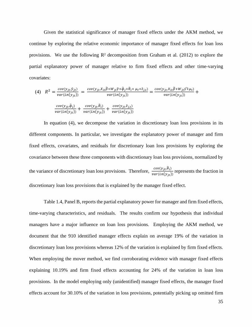
35
Given the statistical significance of manager fixed effects under the AKM method, we
continue by exploring the relative economic importance of manager fixed effects for loan loss
provisions. We use the following R² decomposition from Graham et al. (2012) to explore the
partial explanatory power of manager relative to firm fixed effects and other time-varying
covariates:
(4) 𝑅2 =𝑐𝑜𝑣(𝑦𝑗𝑡,�̂�𝑗𝑡)
𝑣𝑎𝑟(𝐿𝑛(𝑦𝑗𝑡)) =
𝑐𝑜𝑣(𝑦𝑗𝑡,𝑋𝑖𝑡�̂�+𝑊𝑗𝑡�̂�+�̂�𝑗+�̂�𝑖+ 𝜇𝑡+�̂�𝑗,𝑡)
𝑣𝑎𝑟(𝐿𝑛(𝑦𝑗𝑡))=
𝑐𝑜𝑣(𝑦𝑗𝑡,𝑋𝑖𝑡�̂�+𝑊𝑗𝑡𝛾+̂𝜇𝑡)
𝑣𝑎𝑟(𝐿𝑛(𝑦𝑗𝑡))+
𝑐𝑜𝑣(𝑦𝑗𝑡,�̂�𝑗)
𝑣𝑎𝑟(𝐿𝑛(𝑦𝑗𝑡))+
𝑐𝑜𝑣(𝑦𝑗𝑡,�̂�𝑖)
𝑣𝑎𝑟(𝐿𝑛(𝑦𝑗𝑡))+
𝑐𝑜𝑣(𝑦𝑗𝑡,�̂�𝑗,𝑡)
𝑣𝑎𝑟(𝐿𝑛(𝑦𝑗𝑡))
In equation (4), we decompose the variation in discretionary loan loss provisions in its
different components. In particular, we investigate the explanatory power of manager and firm
fixed effects, covariates, and residuals for discretionary loan loss provisions by exploring the
covariance between these three components with discretionary loan loss provisions, normalized by
the variance of discretionary loan loss provisions. Therefore, 𝑐𝑜𝑣(𝑦𝑗𝑡,�̂�𝑖)
𝑣𝑎𝑟(𝐿𝑛(𝑦𝑗𝑡)) represents the fraction in
discretionary loan loss provisions that is explained by the manager fixed effect.
Table 1.4, Panel B, reports the partial explanatory power for manager and firm fixed effects,
time-varying characteristics, and residuals. The results confirm our hypothesis that individual
managers have a major influence on loan loss provisions. Employing the AKM method, we
document that the 910 identified manager effects explain on average 19% of the variation in
discretionary loan loss provisions whereas 12% of the variation is explained by firm fixed effects.
When employing the mover method, we find corroborating evidence with manager fixed effects
explaining 10.19% and firm fixed effects accounting for 24% of the variation in loan loss
provisions. In the model employing only (unidentified) manager fixed effects, the manager fixed
effects account for 30.10% of the variation in loss provisions, potentially picking up omitted firm

36
characteristics. Overall, these findings document a substantial impact of managers on discretionary
loan loss provisions. Furthermore, when we explore the underlying distribution of the manager
fixed effects from the AKM estimation, we find that manager fixed effects are almost normally
distributed showing a significant variation across managers (untabulated).
We next strengthen the robustness of our tests. Therefore, we explore whether the results
are sensitive to the type of included bank managers by exploiting a subsample incorporating C-
level managers only. Table 1.4, Panel C, documents that although the sample size is much smaller
with 196 C-level managers, the explanatory power of manager fixed effects stays largely constant
(partial R²=19.92%) while the firm fixed effect is attenuated to less than 1% (total R²=48.16%).
To further strengthen the robustness of the manager fixed effect estimation, we rerun the AKM
analysis with several additional restrictions in Table 1.5.
Prior studies examining manager fixed effects raise the concern that these effects are
potentially driven by random events during executives’ tenure (Bertrand and Schoar, 2003;
Choi et al., 2015) or endogenous managerial turnover (Fee et al., 2013). Although, this would
affect our results only if employer-employee matching is based on time-varying characteristics that
are not included in the model specification, we address remaining concerns of endogenous sorting
of managers and banks with a subsample analysis including only plausibly exogenous executive
transitions (Fee et al., 2013). However, managers are replaced only in rare cases due to obvious
exogenous reasons such as predecessor death. Following Custodio and Metzger (2014) we collect
plausibly exogenous manager turnovers from retirements. We consider turnovers classified as
“retirement” in ExecuComp or that happen at the age of 61 or older as routine turnovers that are
more likely to be exogenous than a result of the bank replacing a manager in favor of hiring a
manager with a certain loan loss provisioning style.

37
Ta
ble
1.5
R
ob
ust
nes
s te
sts:
eco
no
mic
sig
nif
ica
nce
of
man
ag
er f
ixed
eff
ects
Nu
mb
er o
f
man
ager
FE
Par
tial
R²
exp
lain
ed b
y
man
ager
FE
F-t
est
that
man
ager
FE
=0
(p-v
alu
e)
Par
tial
R²
exp
lain
ed b
y
firm
FE
F-t
est
that
firm
FE
=0
(p-v
alu
e)
Par
tial
R²
exp
lain
ed b
y
tim
e-v
aria
nt
cov
aria
tes
Ad
j. t
ota
l R
²
Ex
og
eno
us
turn
ov
er s
amp
le
12
0
37
.97
%
(0.0
66
) 4
.93
%
(0.1
13
) 1
9.6
0%
5
0.9
4%
At
leas
t tw
o m
ov
ers
per
fir
m
80
5
18
.08
%
(0.0
25
) 1
5.6
1%
(0
.000
) 2
6.2
9%
4
9.1
9%
On
ly t
he
larg
est
con
nec
ted
gro
up
2
98
18
.80
%
(0.0
14
) 1
9.8
6%
(0
.006
) 3
7.8
9%
6
8.8
6%
Sam
ple
sp
lit:
20
01
-20
14
60
3
20
.63
%
(0.0
04
) 1
4.5
4%
(0
.000
) 3
4.0
6%
5
9.6
5%
Ex
clu
din
g 2
00
7/2
00
8/2
00
9
80
6
22
.70
%
(0.0
52
) 1
2.9
9%
(0
.000
) 2
1.6
5%
4
3.2
3%
Tab
le 1
.5 r
eport
s th
e R
² d
ecom
po
siti
on
fro
m e
qu
atio
n (
3)
for
AK
M r
egre
ssio
ns
of
dis
cret
ion
ary l
oan
lo
ss p
rov
isio
ns
on
tim
e v
ary
ing c
on
tro
l v
aria
ble
s
(Reg
ula
tory
Cap
ital
, S
ize,
Mark
et-t
o-B
ook
rat
io,
Ten
ure
, A
ge)
, ti
me
fix
ed e
ffec
ts,
man
ager
fix
ed e
ffec
ts,
an
d f
irm
fix
ed e
ffec
ts w
ith
in f
ive
dif
fere
nt
sam
ple
s. T
he
tab
le s
ho
ws
ho
w m
uch
of
the
var
iati
on
in
sig
ned
dis
cret
ion
ary
lo
an l
oss
pro
vis
ion
s is
ex
pla
ined
man
ager
fix
ed e
ffec
ts,
firm
fix
ed e
ffec
ts,
and
tim
e-v
ary
ing
ch
arac
teri
stic
s. T
he
un
tab
ula
ted
pro
po
rtio
n i
s at
trib
uta
ble
to
res
idu
als.
Th
e F
-tes
t st
atis
tics
ind
icat
e w
het
her
fir
m o
r m
anag
er f
ixed
effe
ct a
re s
tati
stic
ally
sig
nif
ican
tly
dif
fere
nt
fro
m z
ero
. C
riti
cal
val
ues
fo
r th
e F
-sta
tist
ic a
re d
iffe
ren
t ac
ross
mo
del
s d
ue
to d
iffe
ren
t d
egre
es o
f fr
eed
om
.
We
pro
vid
e th
e co
rres
po
nd
ing p
-val
ues
in
par
enth
eses
.

38
Table 1.5 documents the robustness of our findings to this more restrictive sample selection.
Although we can only identify 120 of such plausibly exogenous turnovers, the partial explanatory
power of manager fixed effects for discretionary loss provisioning increases to 38% (p-value<0.1),
whereas firm fixed become statistically insignificant. Therefore, the inference from plausibly
exogenous turnovers supports our prior finding that managers explain a substantial proportion of
the variation in discretionary loan loss provisions, alleviating endogeneity concerns.
We perform four additional robustness tests with different subsamples. First, we ensure the
consistency of our manager fixed effect estimates by including only firms with at least two movers
per bank, and using only the largest connected group for the estimation. Second, we alleviate
concerns that extreme events such as the financial crisis or duration of the sample period affect our
results by first restricting the sample to the 2001-2014 period, and second, excluding the financial
crisis years from 2007-2009. We continue to find that manager fixed effects significantly affect
bank’s loan loss provisioning in all robustness tests, although the economic magnitude of the
manager effects varies slightly between 18% and 23% (p-value<0.01-0.052).
Overall, our results confirm that manager fixed effects play an economically and
statistically significant role in explaining discretionary loan loss provisioning with a partial
explanatory power of approximately 19%. In comparison, time-invariant bank characteristics
explain on average 12% of the variation in discretionary loan loss provisions while further 31% of
the variation are explained by control variables13.
13 The remaining proportion is not explained, therefore reflects the partial explanatory power of residuals. The high
explanatory power of control variables is partly attributable to time fixed effects, added to the time-varying controls
category to avoid overcategorization.

39
1.6. Management styles and the LLP choice
1.6.1. Research design
In the next step of our analysis, we explore whether bank manager’s decision making affects
various bank policy choices in a systematically related way. We start by investigating whether
bank managers fixed effects explain variation for other bank policy choices beyond loan loss
provisions. Specifically, we estimate equation (2) using manager’s compensation incentives, and
loan portfolio choices as dependent variables. We employ Vega, Delta, and total Pay as dependent
variables in equation (2) to capture manger’s intrinsic talent and their risk-preferences from their
market-based compensation (Graham et al., 2012; Albuquerque et al., 2013; Francis et al., 2015).
Furthermore, we capture manager’s idiosyncratic influence on the loan portfolio employing the
Loan-to-Deposit ratio (LtD), the ratio of non-performing loans to gross loans (NPL) and the ratio
of loans to total assets (Loans). Banks with a higher proportion of loans naturally own less
securities, and usually follow a more traditional banking business model (Beltratti and Stulz, 2012).
Furthermore, LtD captures whether loans are funded with deposits or other potentially riskier
sources of funding (Laeven and Levine, 2009). The non-performing loan ratio captures bank’s
non-performing loan classifications as a third important loan portfolio characteristic (Ghosh, 2015).
We employ the AKM method to estimate the manager fixed effects for these six additional policy
choices and to determine how much of the variation is explained by mangers idiosyncratic
influence.
In the next step, we explore whether we find significant correlations across these individual
manager styles for certain bank outcomes. For example, do managers that exert a high influence
over banks loan loss provision also affect non-performing loan classifications? Or do managers

40
with a higher preference for risk-incentivized compensation also express a preference for more
discretionary loan loss provisions? We analyze the correlation structure between manager fixed
effects in the to answer these questions. We then investigate whether individual observable
characteristics explain manager fixed effects and whether we find overarching patterns how
observable manager characteristics influence managerial styles. While many time-invariant
characteristics such as ability, talent or personality are likely difficult to quantify, exploring which
observable factors play a role for bank manager’s accounting and policy decisions is key to the
enhance the understanding of the role of manager characteristics for accounting decisions. 14
Therefore, we estimate the following cross-sectional regressions to test the influence of observable
manager characteristics for the accounting and policy choices:
(4) 𝑀𝑎𝑛𝑎𝑔𝑒𝑟 𝐹𝐸𝑖,𝑘 = 𝑀𝑎𝑛𝑎𝑔𝑒𝑟 𝐶ℎ𝑎𝑟𝑎𝑐𝑡𝑒𝑟𝑖𝑠𝑡𝑖𝑐𝑠𝑖,𝛽 + 𝜙𝑘 + 𝜀i,k
Where i denotes managers and k denotes the AKM estimation group in which we estimated
the manager effect. 𝑀𝑎𝑛𝑎𝑔𝑒𝑟 𝐹𝐸𝑖,𝑘 is the manager fixed effect from the eight different AKM
regressions (equation 2), employing discretionary loan loss provisions (signed and unsigned),
Vega, Delta, Total Pay, Loans, Loans-to-Deposits, and Non-Performing Loans as dependent
variables. 15 Manager Characteristics includes demographic variables (Male, Recession
Executive), occupational status (CEO, CFO, Top Executive), education (Higher Education), and
average risk-taking incentives (Average Delta, Average Vega, Overconfident). In addition, we add
AKM estimation group fixed effects (𝜙𝑘) to account for differences in the estimation group. This
is appropriate because manager fixed effects are estimated within groups of connected managers
14 Graham and Liu (2012) interpret manager fixed effects with management ability and talent, but note that manger
fixed effects capture also all other time-invariant individual attributes. 15 All Variables are defined in Appendix A.
41
and banks and are always estimated relative to the within group before we normalize them. In
addition, we cluster standard errors on the bank level to account for any correlations in managerial
characteristics at the bank level.
Male is an indicator variable that takes the value of one for managers that are male.
Evidence on the influence of gender on corporate decision making is mixed. While Ge et al. (2011)
do not find a significant relation between gender and earnings management, Huang and Kisgen
(2013) document that female executives are more likely to make risky and overconfident corporate
decisions. In contrast, Francis et al. (2015) find that female CFOs tend to increase accounting
conservatism compared to their male peers. Given the mixed evidence on the influence of gender
on accrual quality, we make no ex ante prediction about the influence of gender on loan loss
provisions.
Recession Executive is a binary variable that takes the value of one if the manager started
her career during a NBER-defined recession. Schoar and Zuo (2017) document that an executive’s
management style depends significantly on the market conditions present when the executive enters
the labor market. Their results indicate that CEOs who enter the labor market during a recession
exert a conservative management style with respect to R&D expenditures, capital expenditures and
leverage. Because the career start date is endogenously determined and affected by economic
cycles, we follow their methodology to identify recession executives. First, we add 24 years, the
average age of starting to work at the first position, to the executives’ birth date. Second, we
classify an executive’s first year on the labor market as recession year if it falls at least six months
into a National Bureau of Economic Research-defined recession.

42
In addition, we include binary indicator variables for the exact occupation of the manager
denoting whether the manager is either a CEO, a CFO or another C-level Top Executive. While it
is ex-ante unclear whether CEOs, CFOs or other top executives have the greatest impact on loan
loss provisions, prior literature suggests that CFOs play an incremental role for earnings
management in non-banks (Jiang et al., 2010).
To test if education explains variation in managers’ fixed effects, we collect the highest
degree of the executive and create a binary indicator variable (Higher Education) that takes the
value of one for all managers that have a PhD, MBA or CPA qualification. Education is frequently
employed as a proxy for talent among workers (e.g. Abowd et al., 1999). Furthermore, Bertrand
and Schoar (2003) document a positive impact of managers with MBA qualification on corporate
performance. Nevertheless, prior evidence from Ge et al. (2011) indicates that having a MBA or
CPA qualification does not significantly affect accounting styles in non-banks.
Furthermore, we proxy for managers’ risk-taking incentives using managers average equity
compensation (average Vega and average Delta) incentives over her career. While Vega
theoretically provides clear risk-taking incentives, option Delta has two countervailing effects
(Armstrong et al., 2013). On the one hand, delta incentives risk-taking by rewarding managers
with wealth increases if the stock price accelerates. On the other hand, a higher Delta
simultaneously exposes managers’ wealth to a higher stock-price risk which should reduce risk-
taking. Important to note here is that we use manager’s average Delta and Vega over their whole
sample period while we tease out the time-varying effect of both variables within the AKM
estimation.

43
We include overconfidence as an additional proxy for managers risk-taking incentives. We
employ a binary indicator variable that takes the value of one for managers who do not exercise
stock options that are more than 67% in the money (Campbell et al., 2011). Overconfident
executives are associated with overly optimistic forecasts (Hribar and Yang, 2016) and have a
higher likelihood of intentional misstatements (Schrand and Zechman, 2012).
1.6.2. Results
We first document that managers impose a significant influence over all examined corporate
decisions. Table 1.6, Panel A, shows that manager fixed effects explain between 11.26% and
50.28% of the variation in managements’ policy and accounting styles. Managers fixed effects
seem to matter in particular for compensation and loan portfolio choices. In the next step, we
analyze the correlations across the manager effects for the different corporate decisions. Panel B
reports the pairwise correlations documenting that loan loss provisioning styles are highly
correlated with managements’ idiosyncratic preferences for compensation-based risk-taking
incentives (Vega, Delta, Total Pay) and non-performing loan classifications. This indicates that a
manager’s loan loss provisioning style is associated with preferences for other important corporate
policy choices.
Along these lines, we explore in Panel C whether the correlation in management styles
across different corporate decisions is also reflected in observable manager characteristics that are
captured in the manager fixed effects. To test whether observable manager characteristics affect
corporate choices in a systematic way we regress the manager fixed effects for the corporate choice
on different (time-invariant) observable individual characteristics capturing demographics,
occupational status, education and risk-taking incentives.

44
T
ab
le 1
.6 C
orr
ela
tio
n a
cro
ss m
an
ag
emen
t st
yle
s a
nd
in
div
idu
al
ch
ara
cter
isti
cs
Pa
nel
A:
Eco
no
mic
sig
nif
ica
nce
of
fixe
d e
ffec
ts a
nd
tim
e-va
ryin
g c
ha
ract
eris
tics
fo
r b
an
k p
oli
cy c
ho
ices
Un
sig
ned
DL
LP
Sig
ned
DL
LP
V
ega
D
elta
P
ay
Lo
ans
L
tD
NP
L
Nu
mb
er o
f m
anag
er F
E e
stim
ated
9
11
91
1
93
1
93
1
93
1
93
1
93
1
91
6
Pa
rtia
l R
² ex
pla
ined
by
ma
na
ger
FE
1
1.2
6%
1
9.1
0%
1
9.4
5%
4
6.5
4%
4
8.8
1%
5
0.2
8%
4
4.3
5%
1
2.6
8%
Par
tial
R²
exp
lain
ed b
y f
irm
FE
1
3.8
3%
1
1.8
6%
2
.54
%
4.6
5%
4
.37
%
26
.77
%
42
.82
6.9
9%
Par
tial
R²
exp
lain
ed b
y t
ime-
var
ian
t co
var
iate
s 3
5.6
6%
3
1.3
2%
3
5.6
6%
3
5.8
9%
3
5.7
2%
1
1.5
8%
0
.27
%
58
.43
%
adj.
to
tal
R²
49
.98
%
51
.90
%
46
.16
%
83
.23
%
85
.58
%
85
.54
%
83
.68
%
71
.59
Pa
nel
B:
Pa
irw
ise
corr
ela
tio
ns
acr
oss
dif
fere
nt
ma
na
gem
ent
styl
es
Un
sig
ned
DL
LP
FE
Sig
ned
DL
LP
FE
V
ega
FE
D
elta
FE
P
ay F
E
Lo
ans
Fe
LtD
FE
N
PL
FE
Un
sig
ned
DL
LP
FE
1
.00
00
Sig
ned
DL
LP
FE
0
.51
24
*
1.0
000
Veg
a F
E
0.0
365
*
0.1
781
*
1.0
000
Del
ta F
E
0.2
605
*
0.3
587
*
0.5
656
*
1.0
000
Pay
FE
0
.25
94
*
0.3
222
*
-0.0
28
1
0.1
724
*
1.0
000
Lo
ans
Fe
-0.1
85
2*
0.0
053
0.2
041
*
0.0
757
*
-0.1
78
4*
1.0
000
LtD
FE
0
.05
77
*
-0.1
22
8*
0.1
014
*
0.1
234
*
-0.0
57
7*
0.6
150
*
1.0
000
NP
L F
E
0.5
040
*
0.7
373
*
0.0
517
*
0.3
764
*
0.4
979
*
-0.2
10
8*
-0.1
03
1*
1.0
00
0

45
Ta
ble
1.6
(co
nti
nu
ed)
Pa
nel
C:
Ind
ivid
ua
l ch
ara
cter
isti
cs a
nd
ma
na
gem
ent
styl
es
Un
sig
ned
DL
LP
FE
Sig
ned
DL
LP
FE
V
ega
FE
D
elta
FE
P
ay F
E
Lo
ans
Fe
LtD
FE
N
PL
FE
Dem
og
rap
hic
s
Mal
e 0
.04
3
0.4
00
0.8
89
**
0.3
77
*
0.0
35
-0.0
00
0.0
22
0.0
05
***
(0
.516
) (0
.247
) (0
.011
) (0
.088
) (0
.631
) (0
.981
) (0
.102
) (0
.006
)
Rec
essi
on
Ex
ecu
tiv
e -0
.001
-0.0
98
-0
.051
-0.0
47
-0.0
36
-0.0
00
-0.0
00
0.0
01
(0
.984
) (0
.633
) (0
.861
) (0
.778
) (0
.630
) (0
.944
) (0
.970
) (0
.512
)
Occ
up
ati
ona
l S
tatu
s
CE
O
0.1
18
***
0
.24
8*
-0.0
40
0.1
02
0.5
81
***
-0
.002
0.0
01
0.0
02
*
(0
.000
) (0
.054
) (0
.850
) (0
.265
) (0
.000
) (0
.685
) (0
.873
) (0
.078
)
CF
O
-0.0
05
-0.5
01
**
-0
.550
*
-0.3
37
*
-0.2
30
***
-0
.007
-0.0
28
***
-0
.006
***
(0
.922
) (0
.016
) (0
.067
) (0
.074
) (0
.000
) (0
.316
) (0
.010
) (0
.000
)
To
p E
xec
uti
ve
-0.0
53
-0.3
52
-0
.608
**
-0
.222
0.0
76
-0.0
07
-0.0
17
-0.0
03
*
(0
.389
) (0
.185
) (0
.032
) (0
.128
) (0
.329
) (0
.393
) (0
.153
) (0
.086
)
Ed
uca
tio
n
Hig
her
Ed
uca
tio
n (
Ph
D,
MB
A,
CP
A)
-0.0
34
-0.2
19
-0
.345
-0.1
77
-0.0
16
-0.0
02
-0.0
16
-0.0
03
*
(0
.480
) (0
.179
) (0
.174
) (0
.165
) (0
.834
) (0
.803
) (0
.174
) (0
.069
)
Ris
k-T
aki
ng
In
cen
tive
s
Av
erag
e D
elta
0
.05
9***
0
.46
6***
0
.23
2
0.8
03
***
0
.13
6***
-0
.007
*
0.0
10
0.0
06
***
(0
.010
) (0
.000
) (0
.201
) (0
.000
) (0
.002
) (0
.077
) (0
.125
) (0
.000
)
Av
erag
e V
ega
-0.0
46
**
-0
.182
*
0.4
47
***
-0
.167
***
-0
.045
-0.0
06
*
-0.0
04
-0.0
02
**
(0
.044
) (0
.056
) (0
.002
) (0
.005
) (0
.126
) (0
.074
) (0
.327
) (0
.029
)
Ov
erco
nfi
den
ce
0.0
86
0.5
53
**
0
.68
0***
0
.05
0
0.2
08
***
0
.00
7
0.0
21
0.0
04
***
(0
.149
) (0
.029
) (0
.004
) (0
.546
) (0
.009
) (0
.441
) (0
.147
) (0
.002
)
N
47
29
47
29
47
29
47
29
47
29
47
29
47
29
47
29
Ad
j. R
² 2
6.7
%
29
.1%
1
8.3
%
38
.5%
3
4.4
%
39
.0%
7
0.3
%
40
.5%
Fix
ed E
ffec
ts
26
.4%
2
9.0
%
18
.3%
3
8.5
%
33
.8%
8
3.8
%
69
.1%
4
0.5
%
Clu
ster
B
ank
B
ank
B
ank
B
ank
B
ank
B
ank
B
ank
B
ank
Pan
el A
of
Tab
le 1
.6 r
epo
rts
the
R²
dec
om
po
siti
on
fro
m e
quat
ion
(3)
and
sh
ow
s h
ow
mu
ch o
f th
e v
aria
tio
n i
n b
ank
po
licy
ch
oic
es i
s ex
pla
ined
by
man
ager
fix
ed e
ffec
ts,
firm
fix
ed e
ffec
ts,
tim
e-v
ary
ing
ch
arac
teri
stic
s, a
nd
res
idual
s. W
e u
se t
he
AK
M m
eth
od
an
d r
egre
ss e
ach
po
licy
cho
ice
on
tim
e-v
ary
ing
fir
m a
nd
man
ager
co
var
iate
s
(reg
ula
tory
cap
ital
, m
ark
et-t
o-b
oo
k-r
atio
, si
ze,
age,
ten
ure
) w
ith
tim
e, f
irm
an
d m
anag
er f
ixed
eff
ects
. D
ue
to h
igh m
ult
ico
llin
eari
ty,
we
excl
ud
e ag
e in
th
e P
ay,
LtD
, an
d
NP
L r
egre
ssio
ns.
We
inv
esti
gat
e t
he
foll
ow
ing
po
licy
cho
ices
: u
nsi
gn
ed a
nd
sig
ned
DL
LP
as
pro
xie
s fo
r d
iscr
etio
nar
y l
oan
lo
ss p
rov
isio
ns.
Veg
a, D
elta
an
d P
ay (
tota
l
com
pen
sati
on
) as
co
mp
ensa
tio
n c
ho
ices
. L
oan
s, l
oan
s-to
-dep
osi
ts (
LtD
) an
d n
on
-per
form
ing
lo
ans
(NP
L)
as b
ank
s st
rate
gic
ch
oic
es. A
ll v
aria
ble
s ar
e d
efi
ned
in
Ap
pen
dix
A.
Pan
el B
rep
ort
s p
airw
ise
corr
elat
ion
s ac
ross
man
ager
fix
ed e
ffec
ts (
man
agem
ent
sty
les)
for
the
dif
fere
nt
ban
k p
oli
cy c
ho
ices
fro
m P
anel
A.
Pan
el C
in
ves
tig
ates
th
e
det
erm
inan
ts o
f m
anag
er f
ixed
eff
ects
by
reg
ress
ing
man
ger
fix
ed (
as e
stim
ated
in
Pan
el A
) o
n d
iffe
ren
t ob
serv
able
tim
e-i
nv
aria
nt
man
ager
ch
arac
teri
stic
s. P
-val
ues
are
bas
ed o
n r
ob
ust
sta
nd
ard
err
ors
clu
ster
ed b
y b
ank
. ***,
**,
and
* i
nd
icat
e st
atis
tica
l si
gn
ific
ance
at
the
1%
, 5
%,
and
10
% l
ev
els
(tw
o-t
aile
d),
res
pec
tiv
ely
.

46
We find no significant association between managers’ gender, education, prior crisis
experience and loan loss provisioning styles. However, male managers seem to express a
preference for more risk-taking in the form of higher compensation Vega and Delta. Although
consistent with prior evidence, given the relatively low number of female managers in our dataset,
this finding is not necessarily generalizable to all female managers.
Furthermore, our results suggest that the manager’s exact occupation matters. We
document that CEOs impose the highest influence over (absolute unsigned) loan loss provisions.
In addition, we find that CEOs on average manage loan loss provisions upward whereas CFOs have
an opposing negative influence on provisions. This finding extends prior evidence documenting
that CFOs play an incremental role for earnings management (Jiang et al. 2010). When exploring
other management decisions, we find CEOs to exert more influence over their total pay and non-
performing loans while CFOs have on average significantly lower individual effects on
compensation and loan portfolio characteristics such as loan-to-deposits and non-performing loan
classifications.
Individual risk-taking incentives also affect provisioning styles and loan portfolio choices
significantly. Manager’s average compensation Vega and Delta are also significantly correlated
with manager’s influence on loan loss provisions. Mangers with higher Average Delta exert a
larger idiosyncratic influence on loss provisions whereas managers with higher average Vegas
manage loan loss provisions less. However, managers with higher average compensation Vega on
average influence the loan loss provision downwards. Because we tease out the time-varying effect
of compensation incentives in the AKM regression already, the manager fixed effects capture only
the part of the compensation incentives that relates to manager’s inherent preferences. Along these
lines, we document a preference for a lower loan ratio for managers with high Vega and a less

47
loans classified as non-performing for managers with high Delta. In addition, we do not document
an effect of overconfident managers for absolute loan loss provisions whereas we find that
overconfident managers on average significantly increase loan loss provisions.
Although these results indicate that observable characteristics matter, the correlation of
observable manager characteristics across the different accounting and policy decisions appears to
be little systematic. One potential explanation for this relatively unsystematic correlation is that
observable manager characteristics are unlikely to manifest themselves in isolation and are often
highly correlated. For instance, the choice of the highest degree of an executive is potentially
highly correlated with other executive traits such as intelligence, ability or overconfidence.
Therefore, we employ a Principal Component Analysis (PCA) in the next step of our analysis to
build a composite score capturing the main dimensions of all observable manager characteristics.
Because most characteristics are captured in binary variables, we use polychoric correlations for
the PCA.
The PCA in Table 1.7, Panel A encompasses all manager characteristics from Table 1.6 and
identifies five components with eigenvalues larger than one (Kaiser criterion). In addition, we
build a composite PCA score from these five components that intends to capture a major part of
the variation in observable manager characteristics. We document substantial variation in
component scores for the individual variables across the different components indicating a
successful variance reduction. In Table 1.7, Panel B, we then substitute the individual
characteristics from equation (4) with the five individual PCA components to investigate whether
the combined variation from observable characteristics explains managerial styles for different
policy choices in a systematically related way. The individual PCA components and the composite
PCA score are significantly associated with the manager fixed effect for the different bank policy

48
choices and banks loan loss provisions. Furthermore, we find overarching patterns for the PCA
components and the combined PCA score across the different management styles. This finding is
consistent with the idea that although individual observable characteristics do not explain a large
fraction of the variation in individual manager styles, in combination they are still meaningfully
and systematically correlated with several accounting and policy outcomes.
In the next step, we build on our findings from the prior analyses that latent managerial
styles appear to influence an array of corporate decisions in an interrelated way by constructing
manager profiles based on their revealed individual preferences for the eight different policy
choices. We cluster managers according to their manager fixed effects for the eight corporate
accounting and policy choices to determine a set of unique manager profiles. Using cluster analysis
has the advantage of minimizing variance within clusters while maximizing the variance between
clusters. Specifically, we employ a k-means clustering analysis using the Calinski and Harabasz
(1974) index to determine the number of clusters. We label the groups according to the
classification in Pitcher and Smith (2001) into ‘technocrats’, ‘artists’, ‘craftsmen’, and
‘traditionalists’.

49
Ta
ble
1.7
Cro
ss-s
ecti
on
al
vari
ati
on
of
ma
na
ger
fix
ed e
ffec
ts
Pa
nel
A:
PC
A d
escr
ipti
ve s
tati
stic
s
Co
mp
on
ents
E
igen
val
ue
D
iffe
ren
ce
P
rop
ort
ion
C
um
ula
tiv
e
Co
mp
on
ent
1
2.8
13
1
.49
4
0
.28
1
0
.28
1
Co
mp
on
ent
2
1.3
19
0
.10
8
0
.13
2
0
.41
3
Co
mp
on
ent
3
1.2
11
0
.07
1
0
.12
1
0
.53
4
Co
mp
on
ent
4
1.1
39
0
.06
7
0
.11
4
0
.64
8
Co
mp
on
ent
5
1.0
72
0
.16
4
0
.10
7
0
.75
5
Co
mp
on
ent
6
0.9
08
0
.07
3
0
.09
1
0
.84
6
Co
mp
on
ent
7
0.8
35
0
.41
8
0
.08
4
0
.93
0
Co
mp
on
ent
8
0.4
17
0
.21
3
0
.04
2
0
.97
1
Co
mp
on
ent
9
0.2
04
0
.12
3
0
.02
0
0
.99
2
Co
mp
on
ent
10
0
.08
1
-
0
.00
8
1
.00
0
Var
iab
le
Co
mp
on
ent
1
C
om
po
nen
t 2
C
om
po
nen
t 3
C
om
po
nen
t 4
CE
O
0.4
69
0
.15
2
-0
.243
-0
.429
CF
O
-0.3
25
0
.38
4
0
.48
2
0
.27
0
To
p E
xec
uti
ve
-0.0
99
-0
.705
0
.08
5
0
.35
6
Mal
e 0
.13
6
0
.41
2
0
.39
0
0
.02
9
Lo
wer
Ed
uca
tion
(G
rad
uat
ed)
0.4
82
-0
.158
0
.25
9
0
.01
1
Hig
h E
du
cati
on
(P
hD
, M
BA
, C
PA
) 0
.41
6
-0
.130
0
.47
3
0
.17
7
Rec
essi
on
Ex
ecu
tiv
e 0
.20
7
-0
.055
0
.26
6
-0
.145
Del
ta (
Mea
n)
0.3
69
0
.16
1
-0
.260
0
.44
5
Veg
a (M
ean
) 0
.21
3
-0
.123
-0
.045
0
.14
6
Ov
erco
nfi
den
ce
0.1
31
0
.27
9
-0
.344
0
.58
6

50
T
ab
le 1
.7 (
con
tin
ued
)
Pa
nel
B:
PC
A C
om
pon
ents
and
Ma
na
gem
ent
Sty
les
Un
sig
ned
DL
LP
FE
Sig
ned
DL
LP
FE
V
ega
FE
D
elta
FE
P
ay F
E
Lo
ans
FE
L
tD F
E
NP
L F
E
Co
mp
on
ent
1
0.0
39
***
0
.26
2***
0
.33
2***
0
.37
0***
0
.19
9***
-0
.005
***
0
.00
6*
0.0
03
***
(0
.007
) (0
.000
) (0
.000
) (0
.000
) (0
.000
) (0
.006
) (0
.074
) (0
.000
)
Co
mp
on
ent
2
0.0
51
***
0
.24
3***
0
.17
3**
0.2
08
***
0
.05
1**
0.0
02
0
.00
8**
0.0
02
***
(0
.002
) (0
.001
) (0
.012
) (0
.000
) (0
.019
) (0
.472
) (0
.033
) (0
.000
)
Co
mp
on
ent
3
-0.0
41
**
-0
.307
***
-0
.246
***
-0
.283
***
-0
.152
***
-0
.000
-0
.010
***
-0
.003
***
(0
.013
) (0
.000
) (0
.006
) (0
.000
) (0
.000
) (0
.883
) (0
.003
) (0
.000
)
Co
mp
on
ent
4
0.0
07
0.1
72
**
0.2
83
**
0.2
64
***
-0
.011
-0.0
04
*
0.0
04
0.0
02
***
(0
.728
) (0
.028
) (0
.041
) (0
.000
) (0
.730
) (0
.100
) (0
.416
) (0
.003
)
Co
mp
on
ent
5
-0.0
45
-0.1
46
0.4
89
**
0.1
03
-0.0
56
-0.0
11
**
-0
.006
-0.0
01
(0
.170
) (0
.386
) (0
.015
) (0
.261
) (0
.265
) (0
.022
) (0
.411
) (0
.346
)
N
47
29
47
29
47
29
47
29
47
29
47
29
47
29
47
29
Ad
j. R
² 2
5.9
%
27
.8%
1
6.8
%
28
.8%
3
1.9
%
39
.1%
7
0.1
%
36
.6%
Fix
ed E
ffec
t G
rou
p
Gro
up
Gro
up
Gro
up
Gro
up
Gro
up
Gro
up
Gro
up
Clu
ster
B
ank
B
ank
B
ank
B
ank
B
ank
B
ank
B
ank
B
ank
Pa
nel
C:
PC
A S
core
s a
nd
Man
ag
emen
t S
tyle
s
Un
sig
ned
DL
LP
FE
Sig
ned
DL
LP
FE
V
ega
FE
D
elta
FE
P
ay F
E
Lo
an F
E
LT
D F
E
NP
L F
E
PC
A S
core
0
.06
2*
0.4
38
**
0.7
50
***
0
.71
3***
0
.29
1***
-0
.012
***
0
.00
8
0.0
05
***
(0
.055
) (0
.013
) (0
.000
) (0
.000
) (0
.000
) (0
.004
) (0
.266
) (0
.000
)
N
47
29
47
29
47
29
47
29
47
29
47
29
47
29
47
29
Ad
j. R
² 2
3.8
%
23
.4%
1
1.7
%
19
.2%
2
2.3
%
37
.8%
6
9.4
%
29
.2%
Fix
ed E
ffec
t G
rou
p
Gro
up
Gro
up
Gro
up
Gro
up
Gro
up
Gro
up
Gro
up
Clu
ster
B
ank
B
ank
B
ank
B
ank
B
ank
B
ank
B
ank
B
ank
Pan
el A
of
Tab
le 1
.7 s
ho
ws
des
crip
tiv
e st
atis
tics
for
a p
rin
cip
le c
om
po
nen
ts a
nal
ysi
s o
n a
ll t
ime-i
nv
aria
nt
man
ager
att
rib
ute
s fr
om
Tab
le 1
.6 (
Mal
e, R
eces
sio
n
Ex
ecu
tiv
e, C
EO
, C
FO
, T
op
Ex
ecu
tiv
e, H
igh
er E
du
cati
on
, A
ver
age
Veg
a, A
ver
age
Del
ta,
Ov
erco
nfi
den
ce).
We
use
po
lych
ori
c co
rrel
atio
ns
du
e to
man
y b
inar
y i
np
ut
var
iab
les
to p
erfo
rm t
he
pri
nci
ple
co
mp
on
ent
anal
ysi
s. P
anel
B s
ho
ws
reg
ress
ion
s o
f m
an
ager
fix
ed e
ffec
ts f
or
dif
fere
nt
ban
k p
oli
cy c
ho
ices
on
th
e fi
ve
dif
fere
nt
pri
nci
pal
co
mpo
nen
ts t
hat
cap
ture
var
iati
on
of
the
ind
ivid
ual
ch
arac
teri
stic
s fr
om
Pan
el A
. W
e em
plo
y t
he
Kai
ser
crit
erio
n (
Eig
env
alu
e>1
) as
cu
t-o
ff f
or
sig
nif
ican
t
com
pon
ents
to r
etai
n.
Pan
el C
ag
gre
gat
es t
he
fiv
e co
mp
on
ents
fro
m P
anel
C i
n o
ne
pri
nci
pal
co
mpo
nen
t sc
ore
. P
-val
ues
are
bas
ed o
n r
ob
ust
sta
nd
ard
err
ors
clu
ster
ed
by
ban
k.
***,
**,
and
* i
nd
icat
e st
atis
tica
l si
gn
ific
ance
at
the
1%
, 5
%,
and
10
% l
evel
s (t
wo
-tai
led
), r
esp
ecti
vel
y.

51
In Table 1.8, we descriptively explore the differences in observable manager characteristics
for the four manager clusters. We find that managers labeled as traditionalist are on average
younger, less likely to be overconfident, and have low risk-taking incentives from compensation,
whereas managers labeled as artists are more likely to be overconfident, are more often highly
educated, and have the highest compensation risk-taking incentives. As expected there is
significant variation across manager clusters in the combined PCA score that combines all
observable manager differences.
Table 1.8 Manager profiles
Technocrats Artists Craftsmen Traditionalists
#Managers 253 182 329 147
Manager Characteristics
CEO 0.366 0.446 0.271 0.233
CFO 0.073 0.049 0.151 0.155
Top Executive 0.074 0.069 0.113 0.171
Male 0.914 0.974 0.938 0.888
High Education (PhD,
MBA, CPA) 0.109 0.128 0.074 0.101
Recession Executive 0.154 0.136 0.111 0.120
Delta (Mean) -2.394 -1.644 -2.599 -3.084
Vega (Mean) -3.554 -3.003 -3.375 -4.274
Overconfidence 0.148 0.230 0.137 0.067
Mean PCA Score 0.151 0.459 0.031 -0.302
Age 54.834 56.836 53.017 52.257
Tenure 4.750 6.234 5.780 4.685
Table 1.8 provides summary statistics of the different manager profiles. Manager profiles are determined using a k-means
clustering on all different management fixed effects from Table 6 (DLLP FE, Vega FE, Delta FE, Pay FE, Loans FE,
LtD FE, NPL FE). The optimal number of clusters is determined by the Calinski and Harabasz (1974) index. Mean PCA
score is the average PCA score from Table 1.7, Panel C. All other variables are defined in Appendix A.

52
1.7. Interaction with team composition
1.7.1. Research design
In the following section we investigate whether top management team composition matters
for bank’s loan loss provisioning decisions and how it interacts with individual management styles.
Specifically, we explore whether different manager types influence the bank’s accounting choices
and how the effect is altered by heterogeneity at the top management team level. Therefore, we
estimate the following model:
(5) 𝑃𝑜𝑙𝑖𝑐𝑦 𝐶ℎ𝑜𝑖𝑐𝑒𝑖,𝑗,𝑡 = 𝑀𝑎𝑛𝑎𝑔𝑒𝑟 𝑇𝑦𝑝𝑒𝑖,𝑗,𝑡𝛽 + 𝐷𝑖𝑣𝑒𝑟𝑠𝑒 𝑇𝑀𝑇𝑗,𝑡𝛾
+ 𝐷𝑖𝑣𝑒𝑟𝑠𝑒 𝑇𝑀𝑇𝑗,𝑡 ∗ 𝑀𝑎𝑛𝑎𝑔𝑒𝑟 𝑇𝑦𝑝𝑒𝜙𝑖,𝑗,𝑡 + 𝜃𝑖 + 𝜇𝑡 + 𝜙𝑗 + 𝜀𝑖,𝑗,𝑡
As dependent variable we use all accounting and corporate policy choices from Table 6,
Panel A. Therefore, the dependent variable is the time-varying corporate choice.
𝑀𝑎𝑛𝑎𝑔𝑒𝑟 𝑇𝑦𝑝𝑒𝑖,𝑗,𝑡 denotes and indicator variable for the four unique manager types we identify
in the cluster analysis from Table 8. Managers labeled as ‘Traditionalist’ serve as the reference
group in all tests. We include a binary variable 𝐷𝑖𝑣𝑒𝑟𝑠𝑒 𝑇𝑀𝑇𝑗,𝑡 that indicates whether at least two
different manager types (Technocrat, Artist, Craftsmen or Traditionalist) are represented in the top
management team. Furthermore, we include size, regulatory capital, and the market-to-book ratio
to capture time-varying firm characteristics. In addition, we include firm- and year-fixed effects
to account for unobserved heterogeneity on the year and bank level. In all our tests, we draw
statistical inferences based on standard errors clustered by bank to control for time-series
correlation (Petersen, 2009).

53
1.7.2. Results
We report the results for the impact of different manager types and top management team
heterogeneity in Table 1.9. Managers that we label as artists and technocrats exert on average a
higher discretion over the loan loss provision after controlling for bank characteristics, year, and
bank fixed effects. Furthermore, artist managers are also associated with a preference for higher
risk-taking incentives from compensation (Vega). In addition, we document a positive baseline
effect of Diverse TMT. That is, team diversity does not seem to be associated with less
discretionary loss provisions per se. However, diversity is on average rather associated with
overprovisioning than with risky underprovisioning. Furthermore, we document that top
management team diversity can attenuate the negative effect of technocrats and artists on loan loss
provision quality. This beneficial effect of top management team diversity is particularly
pronounced in teams that include risk-seeking managers that we label as artists. Overall, our results
document that diversity within top management teams can moderate the significant association
between individual manager styles and the level of reporting discretion. Therefore, top
management team diversity can help reducing reporting discretion for manager types that are most
prone to making risky provisioning and loan portfolio decisions.

54
Ta
ble
1.9
To
p m
an
ag
emen
t te
am
com
po
siti
on
an
d b
an
k o
utc
om
es
Un
sig
ned
DL
LP
Sig
ned
DL
LP
V
ega
Del
ta
Pay
L
oan
s L
tD
NP
L
Tec
hn
ocr
ats
0.5
55
***
3
.60
7**
4
.68
2
1.3
62
***
0
.19
1
0.1
09
***
0
.14
2***
0
.01
4
(0
.004
) (0
.015
) (0
.107
) (0
.000
) (0
.268
) (0
.004
) (0
.003
) (0
.169
)
Art
ists
0
.57
2***
3
.20
5**
6
.43
3**
2.6
29
***
0
.25
9
0.0
25
0.0
22
0.0
12
(0
.006
) (0
.022
) (0
.030
) (0
.000
) (0
.205
) (0
.401
) (0
.654
) (0
.263
)
Cra
ftsm
en
0.1
34
1.1
38
5.5
86
*
1.3
85
***
0
.05
5
-0.0
06
0.0
19
0.0
06
(0
.382
) (0
.392
) (0
.059
) (0
.000
) (0
.770
) (0
.796
) (0
.612
) (0
.548
)
TM
T D
iver
sity
0
.30
8**
2.2
45
*
2.9
97
0.2
93
-0.1
68
0.0
09
0.0
30
0.0
13
(0
.013
) (0
.089
) (0
.313
) (0
.163
) (0
.238
) (0
.665
) (0
.215
) (0
.195
)
Tec
hn
ocr
at *
Div
erse
TM
T
-0.3
84
**
-2
.747
*
-3.3
29
-0.2
13
0.1
26
-0.1
06
***
-0
.135
***
-0
.013
(0
.037
) (0
.068
) (0
.260
) (0
.348
) (0
.428
) (0
.004
) (0
.005
) (0
.193
)
Art
ist
* D
iver
se T
MT
-0
.581
***
-3
.050
**
-3
.284
-0.4
38
*
0.4
20
**
-0.0
21
-0.0
17
-0.0
14
(0
.004
) (0
.029
) (0
.264
) (0
.080
) (0
.012
) (0
.413
) (0
.670
) (0
.204
)
Cra
ftsm
en *
Div
erse
TM
T
-0.1
32
-1.3
50
-3.3
29
-0.3
83
0.1
70
0.0
09
-0.0
12
-0.0
09
(0
.392
) (0
.318
) (0
.254
) (0
.125
) (0
.264
) (0
.686
) (0
.717
) (0
.389
)
Reg
ula
tory
Cap
ital
-0
.230
*
-1.0
44
0.6
42
*
0.8
66
***
0
.20
0**
-0.0
63
**
-0
.050
-0.0
15
***
(0
.073
) (0
.162
) (0
.074
) (0
.000
) (0
.018
) (0
.021
) (0
.179
) (0
.000
)
Siz
e -0
.075
-0.3
52
0.8
14
***
0
.42
9***
0
.34
6***
-0
.026
0.0
53
*
-0.0
05
**
(0
.383
) (0
.220
) (0
.000
) (0
.000
) (0
.000
) (0
.169
) (0
.054
) (0
.022
)
MtB
-0
.096
*
-0.9
63
***
0
.03
4
0.2
42
***
0
.18
1***
-0
.003
-0.0
10
-0.0
06
***
(0
.099
) (0
.000
) (0
.795
) (0
.005
) (0
.000
) (0
.785
) (0
.487
) (0
.000
)
N
47
29
47
29
47
29
47
29
47
29
47
29
47
29
47
29
Ad
j. R
² 5
1.0
%
49
.0%
3
6.6
%
57
.3%
6
5.6
%
77
.5%
7
5.8
%
65
.6%
Fir
m &
Yea
r F
E
Yes
Y
es
Yes
Y
es
Yes
Y
es
Yes
Y
es
Clu
ster
B
ank
B
ank
B
ank
B
ank
B
ank
B
ank
B
ank
B
ank
Tab
le 9
sh
ow
s re
gre
ssio
ns
of
dif
fere
nt
ban
k p
oli
cy c
ho
ices
on
in
dic
ato
r v
aria
ble
s fo
r th
e d
iffe
ren
t m
anag
er p
rofi
les.
Tec
hn
oc
rats
, A
rtis
ts,
Cra
ftsm
en,
and
Tra
dit
ion
alis
ts
are
ind
icat
or
var
iab
les
for
dif
fere
nt
man
ager
pro
file
s fr
om
the
k-m
ean
s cl
ust
erin
g i
n P
anel
A. T
rad
itio
nal
ists
ser
ve
as t
he
refe
ren
ce g
roup
. T
he
op
tim
al n
um
ber
of
clu
ster
s
is d
eter
min
ed b
y a
k-m
ean
s cl
ust
erin
g a
nd
th
e C
alin
ski
and
Har
abas
z (1
97
4)
ind
ex.
Div
erse
TM
T i
s a b
inar
y i
nd
icat
or
var
iab
le t
hat
tak
es t
he
val
ue
of
on
e fo
r a
top
man
agem
ent
team
th
at c
on
sist
ou
t o
f m
ore
th
an o
ne
par
ticu
lar
man
ager
ty
pe.
P-v
alu
es a
re b
ased
on
ro
bu
st s
tan
dar
d e
rro
rs c
lust
ered
by
ban
k.
**
*,
**,
and
* i
nd
icat
e
stat
isti
cal
sig
nif
ican
ce a
t th
e 1%
, 5
%,
and
10
% l
evel
s (t
wo
-tai
led
), r
esp
ecti
vel
y.

55
1.8. Conclusion
This study explores the role of manager characteristics and top management team
composition for banks’ loan loss provisions. While prior literature documents that bank-specific
incentives and variation over time shape loan loss provisions, we are the first to show a significant
idiosyncratic manager effect for this major accounting choice. Nevertheless, our tests reveal that
observable compensation and manager characteristics explain only a small fraction of banks loan
loss provisioning behavior. The low correlations between observable characteristics and reporting
outcomes, however, do not imply that individual bank managers have little influence on accounting
choices. Managers exert influence in an idiosyncratic way through their preferences, skills, or
values that are inherently difficult to measure but important to understand a managers’ role in the
accounting process.
Exploiting a large sample of connected managers and banks, we document that after
accounting for firm and time differences manager characteristics explain approximately 19% of the
variation in the discretionary loan loss provision. We use plausibly exogenous turnovers as a
setting to corroborate these findings and to document that manager fixed effects are not a mere
outcome of firm policy changes. Furthermore, manager styles for different corporate policies are
systematically correlated. For example, managers employing high discretion in the loan loss
provisioning choice also prefer a higher level of risk-taking and, on average, a lower quality of the
loan portfolio. That is, managers who have a distinct impact on the loan loss provisioning do exert
their influence on other corporate actions in a systematically related way. Using these systematic
correlations across manager styles we cluster managers into four unique types. We document that
particularly managers whom we label as artists and technocrats use discretion over the loan loss
provision. In addition to the individual manger effects we document that top management team

56
composition can significantly alter the impact of individual managers. Our results provide
evidence that top management team diversity mutes the idiosyncratic influence of managers that
employ the most aggressive loan loss provisioning styles.
Overall, our findings imply that bank supervisor’s focus on skills and qualifications of
individual managers can be only partially justified by the relatively limited systematic impact that
individual observable characteristics have on relevant corporate policies. However, the focus on
individual managers is necessary as a large proportion of bank’s policy choices is attributable to
individual management styles. Furthermore, idiosyncratic manager influence seems to interact
strongly with the combination of manager types within the top management team providing some
support for regulation to increase the top management team diversity.

57
1.9. Appendix A: Variable definitions
Manager
Variables Description Source and computation
Age Executives' Age in years ExecuComp
Tenure Duration of the employment on the current
position ExecuComp
Male Indicator variable for male managers ExecuComp
Salary Total fixed Salary ExecuComp: Natural logarithm of fixed salary
Bonus Bonus ExecuComp: Natural logarithm of bonus
Total Pay Total Salary and Bonus Execucomp: Natural logarithm of total compensation
Vega Dollar change in wealth linked to a 1% increase
in stock return volatility
Coles, Daniel and Naveen (2006):
Scaled with total cash compensation and log
transformed (Edmans, 2009)
Delta
Dollar change in manager’s
wealth to changes in a bank’s stock price
performance
Coles, Daniel and Naveen (2006):
Scaled with total cash compensation and log
transformed (Edmans, 2009)
CEO Indicator for manager’s occupation Execucomp/Boardex
CFO Indicator for manager’s occupation Execucomp/Boardex
Top
Executive Indicator for manager’s occupation
Execucomp/Boardex: Top 5 executive classified as
CEO,CFO,CRO,CIO or COO
Recession
Executive
Indicates managers that started
their career during a recession
Execucompt Birthdate + 24 years within NBER-
defined recession
Higher
Education
Indicator variable for managers with
PhD, CPA or MBA qualification Boardex
Over-
confidence Indicator for overconfident managers
Indicator for unexercised stock options more than
67% in the money
Bank
Variables Description Source and computation
MtB Market to book ratio
Compustat: Market value of equity divided by the
book value of equity(common shares
outstanding*price/common equity)
Size Size Compustat: Natural logarithm of total assets
LLP Loan loss provisions Compustat: Loan loss provisions scaled by lagged
total loans
Regulatory
Capital Tier 1 regulatory capital Compustat: Natural logarithm of tier 1 capital
NPL Non-performing loans Compustat: Non-performing loans scaled by lagged
total loans
CO Charge-offs Compustat: Charge-offs scaled by lagged total loans
ALW Allowance for loan losses Compustat: Loan loss allowance scaled by total loans
EBLLP Earnings before loan loss provisions Compustat: (Earnings + loan loss provisions) scaled
by lagged total loans
LtD Loans-to-Deposits Compustat: Total loans scaled with total deposits
NPL Non-performing loans ratio Compustat: Non-performing loans scaled with total
loans
Loans Total loans ratio Compustat: Total loans scaled with total assets
HPI House price index Federal Housing Finance Agency
GDP Gross domestic product Federal Reserve bank of St. Louis
58
Chapter 2
Do Supervisory Disclosures Lead to Greater Bank Transparency?
The Role of Enforcement and Market Discipline
“One of the outcomes we expect from these tests is to dispel this fog that lies over bank balance
sheets in the Euro area and in Europe.”
Mario Draghi, 23/10/2013, in a speech to the European Parliament
2.1. Introduction
Supervisors can influence the reporting behavior of supervised firms through different
channels. Their public enforcement relies on direct interventions such as comment letters,
supervisory instructions, or fines (Jackson and Roe, 2009). However, they can also disclose private
information to the public to increase market attention and encourage third-party monitoring (Duro,
Heese, and Ormazabal, 2019). Such supervisory disclosures can also serve as a commitment device
to assure supervisory discipline (Bushman and Williams, 2012; Dudley, 2009). In the banking
industry, the role of supervisory disclosures about the financial health, risk, and transparency of
regulated banks is controversial (Goldstein and Sapra, 2014). Enhanced disclosures equip market
participants with a better understanding of bank fundamentals and thus help establish market
discipline (Berger, Davies, and Flannery, 2000; Flannery, 2001; Herring, 2004), but increased
transparency potentially mitigates opportunities for regulators to practice forbearance behind the
scenes (Gallemore, 2019; Skinner, 2008). Therefore, ex ante it is not clear whether supervisory
reporting preferences are in line with market demand for bank transparency, and how supervisory
disclosures interact with traditional enforcement in increasing bank transparency.

59
The European Central Bank’s (ECB) Asset Quality Review (AQR) provides a useful setting
to explore the financial reporting preferences of bank regulators and the complementary roles of
traditional enforcement and supervisory disclosures. In the run-up to the European Single
Supervisory Mechanism (SSM), which shifted the responsibility for the prudential supervision of
the most significant Eurozone banks from national regulators to the ECB, the ECB reassessed the
audited financial statements of each affected bank and published its findings.16 For example, the
ECB revealed that it viewed banks’ loan loss allowances to be understated by, on average, 25%
(median: 8%). However, most of the AQR adjustments were not due to formal violations of
accounting rules, but rather signaled a shift in supervisory reporting preferences within a common
accounting framework, with the ECB generally preferring higher levels of provisioning than the
national supervisors previously in charge of bank supervision.
This paper explores the effect of these changes in the reporting preferences of the
responsible supervisor and the corresponding supervisory disclosures. In particular, we address
three research questions. First, we examine whether banks adjust their reporting behavior following
the change of their responsible supervisor and the public assessment of their asset quality. Second,
we investigate whether the change in supervisory responsibility is also associated with the market
perception of bank transparency as reflected in lower information asymmetry and greater market
liquidity. Third, we compare how the changes in reporting behavior and perceived transparency
relate to both the shift in supervisory authority and third-party market monitoring.
We exploit the data made available by the ECB as part of the AQR exercise to address these
questions. These supervisory disclosures provide a relatively clean measure of firm-level
16 In addition to the Asset Quality Review, this Comprehensive Assessment (CA) included a stress test.

60
differences in regulatory reporting preferences, and ultimately regulatory scrutiny, between the
prior national supervisors and the ECB. This is important because, across the board, the ECB is
not a stricter supervisor per se.17 The availability of a firm-level measure of changes in regulatory
scrutiny differentiates our paper from prior studies on the effect of supervisory characteristics on
bank reporting. Observable differences across regulatory regimes used in the literature are likely
not only driven by supervisory characteristics, but also by macroeconomic conditions, idiosyncratic
portfolio choices, and reporting incentives (Costello, Granja, and Weber, 2020; Nicoletti, 2018).
Even for intra-firm changes in supervisory institutions, differences in supervisory characteristics
need not uniformly affect supervised institutions (Agarwal, Lucca, Seru, and Trebbi, 2014; Granja
and Leuz, 2019). For example, small banks with a straightforward business model can be
supervised equally well by regulators with and without extensive resources. Similarly, concerns
about regulatory capture that result from reputational concerns or future employment opportunities
plausibly differ in the cross-section of banks.
In the first step of our analyses, we employ a panel of yearly bank-level accounting data
over the period from 2011 to 2017 (i.e., three years before and three years after the introduction of
the SSM in the Eurozone). To examine banks’ reporting behavior, we focus on changes in loan
loss provisioning and the classification of non-performing loans. Our research design benefits from
the national regulators remaining responsible for the supervision of non-SSM banks. We include
all other European banks that overlap in size with the SSM treatment sample as a benchmark group
17 For example, Nordea, the largest bank in Sweden (which is not part of the Eurozone), relocated its headquarters
from Stockholm to Helsinki in late 2018 in a conscious effort to fall under SSM supervision instead of the
Swedish Finansinspektionen (Financial Times, 2017).

61
to enable a difference-in-differences estimation that controls for general time trends and macro-
level shocks.
Controlling for changes in the underlying risk of the loan portfolio, we find, if anything, a
negative standalone effect of SSM supervision on the level of loan loss provisions and non-
performing loans. For instance, the ratio of non-performing to total loans decreased by 1.2
percentage points for SSM banks after becoming subject to ECB supervision, which amounts to
about 18% of the average non-performing loan ratio of all banks in our sample period. This is in
contrast to the common notion that the ECB is a generally stricter supervisor than the prior national
regulators (Fiordelisi, Ricci, and Lopes, 2017), and is consistent with our understanding that the
impact of the SSM is not uniform across all affected banks, but depends on the firm- and country-
specific divergences in supervisory policy. Consequently, when we take the magnitude of the AQR
adjustments into account, we find that against the negative base effect, reporting conservatism
significantly increases with larger adjustments. We interpret this as evidence that banks’ reporting
choices are influenced by supervisory preferences beyond simple compliance with given
accounting standards.
In the second step, we estimate panel regressions of monthly bid-ask-spreads as a proxy for
market liquidity and information asymmetry among market participants for the subsample of listed
treatment and control firms. We find that the SSM adoption is associated with a decrease in the
bid-ask spreads of participating banks by about 16%. However, when we interact the SSM
participation with the magnitude of a bank’s AQR adjustment, we observe that this association is
limited to those banks with greater AQR adjustments. This finding supports the view that
supervisory scrutiny can reduce information asymmetry and contribute to a higher level of
perceived transparency.

62
In the third step, we examine the cross-sectional variation in the changes in reporting
behavior and market liquidity around the SSM adoption more closely. In particular, to gauge the
relative importance of enforcement and market discipline, we test to what extent the changes are
attributable to supervisory reporting preferences (i.e., differences between the ECB and the national
supervisor) or to the strength of market forces at the firm level. We find that the likelihood of
political capture under local regulation and the increase in the quality of the regulatory
infrastructure are associated with the change in banks’ reporting behavior. Banks that are subject
to the greatest shift in these supervisory characteristics exhibit the strongest increase in loan loss
provisions and loans classified as non-performing. However, we fail to find evidence that an
increase in regulatory scrutiny per se also translates into higher stock liquidity. Instead, rather than
with regulatory characteristics, the changes in market liquidity around SSM adoption are associated
with the strength of third-party market monitoring through, e.g., depositors and other providers of
bank funding. The latter finding implies that even where supervisory action is not perfectly aligned
with market demand for information, supervisory disclosures like the publication of the AQR
results can stimulate market discipline and push banks to increase their level of transparency.
Our study contributes to different streams of the literature. First, it is related to research on
the influence of supervisory institutions and their enforcement on reporting outcomes and firm
transparency in general and, in particular, in the banking industry (Bischof, Daske, Elfers, and Hail,
2020; Costello et al., 2016; Granja, 2018; Granja and Leuz, 2019; Leuz and Wysocki, 2016;
Nicoletti, 2018). We add to this literature by focusing on a clearly identified setting that is
characterized by within-firm changes in the responsible supervisor and a firm-level measure of
supervisory reporting preferences that captures variation in the potential impact of the reform. Our
results on the institutional determinants of the SSM/AQR effect are also related to the literature on

63
the consequences of intra-agency and interagency heterogeneity for regulatory outcomes (Busuioc,
2015; Fremeth and Holburn, 2012; Macher, Mayo, and Nickerson, 2011) and on political influence
and regulatory capture (Agarwal, Amromin, Ben-David, and Dinc, 2018; Lambert, 2018).
Second, our paper adds to the literature on the effects of supervisory disclosure. In particular
in the banking industry, disclosures about enforcement actions or regulatory stress tests have been
found to be informative and to elicit market discipline by investors (Petrella and Resti, 2013;
Morgan, Peristiani, and Savino, 2014; Flannery, Hirtle, and Kovner, 2017; Fernandes, Igan, and
Pinheiro, 2017). These disclosures can also have feedback effects on the supervisor’s choice of
enforcement actions (Kleymenova and Tomy, 2020) and on firms’ reporting behavior (Bischof and
Daske, 2013; Duro et al., 2019). We complement these studies by investigating under which
conditions supervisory disclosure can facilitate changes in banks’ reporting behavior and perceived
transparency.
Finally, our paper adds to the topical literature on the SSM. Prior research focuses either
on the determinants (Acharya and Steffen, 2014; Homar, Kick, and Salleo, 2015; Steffen, 2014) or
on the immediate market reaction to the publication of the results of the AQR and the
contemporaneous stress test (Carboni, Fiordelisi, Ricci, and Lopes, 2017; Lazzari, Vena, and
Venegoni, 2017; Sahin and de Haan, 2016). Regarding the real effects of the SSM adoption,
Fiordelisi et al. (2017) document that affected banks reduced their credit supply in the run-up to
the SSM launch to improve their equity capital ratios.18 Our study contributes to this literature by
18 Eber and Minoiu (2017) also find that banks subject to the Comprehensive Assessment adjusted their leverage,
mainly by reducing lending and wholesale funding. Gropp, Mosk, Ongena, and Wix (2019) make a similar point
regarding the 2011 stress test by the European Banking Authority (EBA).

64
providing evidence on how the SSM influenced the long-term transparency of supervised
institutions.
The remainder of the paper proceeds as follows. In Section 2, provide more details on the
SSM and the AQR disclosures and develop our empirical predictions. In Section 3, we outline the
research design, describe the sample selection, and provide descriptive statistics. Section 4 presents
the results of the baseline analysis of the SSM/AQR effects on banks’ accounting behavior and
perceived transparency, and the cross-sectional tests along the dimensions of changes in
supervisory enforcement and the intensity of market monitoring. Section 5 concludes.
2.2. Institutional setting and empirical predictions
2.2.1. Bank supervision and accounting enforcement under the Single Supervisory Mechanism
To reinstate trust in the financial markets after the European sovereign debt crisis,
policymakers and regulators called for a coordinated approach regarding the governance of
financial system stability. A major aspect of these initiatives was the integrated supervision of
cross-border banking activities, as banking supervision was predominantly performed by national
supervisors even for large, internationally active banking groups.19 To facilitate the harmonization
19 National supervisors of cross-border banking groups were already engaging in information sharing in the form
of “supervisory colleges” before the crisis. These supervisory colleges were formed to foster coordination
between the different national supervisors and were formally mandated by the EU Capital Requirements Directive
II (Directive 2009/111/EC). However, the degree of collaboration between national supervisors within the
colleges varied significantly, often leading to inefficient microprudential supervision. For instance, during the
chaotic bailout of the Fortis banking group, regulators from Belgium, Luxemburg, and the Netherlands had
difficulties to align their actions (Financial Times, 2009).
65
of the European system of banking supervision, the Eurozone countries formally agreed to form a
Banking Union in December 2012.
This Banking Union consists of three building blocks: the SSM, the Single Resolution
Mechanism, and a common deposit insurance scheme. Under the SSM, the ECB formally assumed
responsibility as the prudential supervisor of all banks in the Eurozone as of November 2014
(Regulation EU/1024/2013). At the same time, the ECB automatically redelegated the supervision
of all “non-significant” institutions back to the originally responsible national supervisors.20 The
ECB determines the significance of a bank on a country-by-country basis depending on
predetermined size cutoffs (total assets above EUR 30 billion or the bank being among the three
largest financial institutions of a country) and the extent of its cross-border activities. As such,
with the adoption of the SSM regulation, the ECB became the direct supervisor of 120 major
financial institutions in 18 Eurozone countries (plus Lithuania, which adopted the Euro in 2015),
aiming to “build on the best supervisory practices that are already in place” (ECB, 2014a).
Prudential supervision for these significant institutions is carried out by joint supervisory teams
composed of both supervisory staff directly employed by the ECB and representatives assigned
from the national supervisors of countries where the bank has subsidiaries or significant branches.
To impede regulatory capture, team members rotate on a regular basis (ECB, 2018b). Although
the ECB sets the supervisory agenda and the joint supervisory teams are always headed by ECB
20 The General Court of Justice eventually ruled that national authorities had no formal autonomous competence
for prudential supervision of euro area financial institutions (Case T-122/15 Landeskreditbank Baden-
Württemberg vs. ECB, 2017). However, once prudential supervision tasks were redelegated to a national
supervisor, there was no formal accountability mechanism that would give the ECB any power to sanction the
national supervisor besides the latent threat to reassume the role of the supervisor of a less significant institution
in the respective country (Karagianni and Scholten, 2018).

66
staff, the teams rely extensively on the national supervisor’s existing supervisory infrastructure as
well as on their local staff in their operations (European Court of Auditors, 2016; IMF, 2018).
On October 26, 2014, shortly before the introduction of the SSM, the ECB and the European
Banking Authority (EBA) released the results of a Comprehensive Assessment (CA) that consisted
of the AQR and a stress test of major Eurozone banks.21 While the stress test gauged the banks’
resilience against macroeconomic shocks, the AQR involved a detailed review of bank balance
sheets with the objective of harmonizing the measurement of banks’ risk exposures and increasing
the quality of public information. In particular, the AQR assessed the adequacy of loan loss
provisions, collateral valuations, and the classification of loan exposures as non-performing. It was
a supervisory exercise of unprecedented scale (ECB, 2014b), lasting 12 months, involving more
than 6,000 staff, and costing nearly EUR 500 million for external auditors and consultants. In 2015
and 2016, the EBA carried out two more AQRs to prepare the inclusion of additional banks to the
SSM supervisory system (2015: 13 banks, 2016: 3 banks). Importantly, the ECB did not intend
the findings of the AQR to trigger immediate accounting restatements, and only 8% of the
additionally required loan loss provisions were stated to stem from actual violations of binding
accounting rules (ECB, 2014b). Instead, the AQR adjustments revealed differences in the
regulatory reporting preferences between the ECB and individual national regulators that originate
from the discretion inherent to the application of financial reporting standards for loan loss
provisioning.
21 While there was significant overlap between CA inclusion and participation in the SSM, some banks did not
become subject to ECB supervision but were part of the AQR, and vice versa. Specifically, between 2014 and
2017, 136 banks were included in the SSM, but seven of these were never included in an AQR. In the AQRs, the
ECB assessed 142 banks, but 13 of these AQR banks were never included in the SSM. Therefore, the overlap
between SSM and AQR comprises a set of 129 banks (see Table 1 for details).

67
2.2.2. Banks’ reporting behavior around the supervisory AQR disclosures
Formal supervisory enforcement and informal supervisory influence are an important
determinant of firms’ reporting behavior (Christensen, Hail, and Leuz, 2013; Gipper, Leuz, and
Maffett, 2019; Holthausen, 2009). In the banking sector, bank supervisors tend to dominate the
public enforcement of reporting regulation. They have economic resources and legal powers that
usually outmatch those of general accounting supervisors (such as the securities market regulator)
by a wide margin (Bischof et al., 2020). However, bank supervisors can have ambiguous
preferences regarding bank transparency, which are not necessarily aligned with investors’ demand
for information. For example, supervisors prefer at least some specific banks to be opaque to
facilitate the orderly resolution of troubled institutions, to avoid market concern, or to protect the
supervisor’s reputation (Gallemore, 2019; Steffen, 2014).
We expect that the transnational unification of supervisory institutions under the SSM
affects bank reporting, beyond formal compliance with accounting standards, through a
harmonization of these supervisory preferences. Importantly, this effect is not necessarily uniform
at the individual firm level, but depends on the relative divergence in supervisory reporting
preferences between the national regulator and the ECB, which becomes manifest in the bank-
specific AQR adjustment. We therefore predict that SSM banks will adjust their accounting policies
corresponding to the magnitude of these published accounting adjustments.
The extent to which the ECB will intervene and enforce its reporting preferences likely
depends on a country’s specific institutional setup, such as the sources of the national supervisor’s
prior leniency and the national supervisor’s relative resources and bargaining power. Supervisory
leniency can be caused by a lack of supervisory resources, which reduces the ability to detect
68
shortcomings and to enforce corrective action (Fremeth and Holburn, 2012; Jackson and Roe,
2009; Macher et al., 2011). At the same time, the national supervisors’ endowment and ability also
likely determine their bargaining power in determining supervisory policies relative to the ECB,
which initially had to rely substantially on local resources and the existing supervisory
infrastructure (European Court of Auditors, 2016; IMF, 2018). Against this backdrop, we predict
that the adjustment of banks’ accounting behavior is more pronounced in countries with relatively
weak national supervisors.
Another important potential cause of supervisory leniency is institutional capture (Lambert,
2018; Macher and Mayo, 2012; Stigler, 1971). As the ECB is a relatively independent institution
regarding the influence of individual governments or national interest groups (Loipersberger,
2018), the SSM implementation likely mitigates such issues, and we expect that SSM banks are
required to adjust their accounting policies more strongly in local environments that indicate prior
capture of the national supervisor.
In addition to the direct intervention by the supervisor, we expect that the SSM
implementation also affects banks’ reporting behavior indirectly through market pressure that
stems from the disclosure of the AQR results. Such supervisory disclosure provides market
participants with private supervisory information and allows them to impose market discipline on
the supervised firms, which in turn can induce changes in firm behavior (Duro et al., 2019). The
more a bank’s funding structure or the perceived threat of distress facilitate market monitoring, the
greater we expect banks to adjust their reporting choices.

69
2.2.3. Bank transparency around the supervisory AQR disclosures
Where the AQR adjustments match market concerns about banks’ portfolio risk
(Carboni et al., 2017; Lazzari et al., 2017), their publication and the corresponding changes in
reporting behavior can increase banks’ perceived transparency and, through the reduction in
adverse selection, induce an increase in stock liquidity (Diamond and Verrecchia, 1991; Leuz and
Verrecchia, 2000; Verrecchia, 2001). In addition, even if the AQR adjustments are not fully
aligned with investors’ informational needs (e.g., because they are understood simply as an
indicator of unconditional supervisory conservatism), they can suggest a higher level of
supervisory strictness under the SSM that might affect the perception of banks’ reporting quality
in general. Similarly, supervisory disclosures that reveal substantial AQR adjustments likely trigger
investor attention that extends to all aspects of financial reporting, which in turn can generate
market pressure for banks to increase their overall level of public information.
2.3. Research design and data
In this section, we describe the empirical identification strategy and develop the regression
models to test our main predictions regarding the effect of the SSM introduction and the
supervisory AQR disclosures on bank’s reporting behavior and, consequently, on market liquidity.
We then discuss the sample selection and provide descriptive statistics on our sample of European
banks.
2.3.1. Empirical model
We evaluate the changes in bank reporting and transparency around the SSM adoption and
after the supervisory AQR disclosures from two perspectives. First, we analyze changes in banks’

70
loan loss reporting behavior around the AQR disclosures using panel regressions with different key
ratios from banks’ yearly financial statements as the dependent variable. Second, we examine
whether the observed changes in reporting behavior are associated with an increase in bank
transparency and lower levels of information asymmetry (as reflected in bid-ask spreads). The
analyses rely on publicly available data on the AQR adjustments. These adjustments provide us
with a granular and firm-specific measure of the extent to which the newly adopted supra-national
SSM supervision reflects a change in supervisory reporting preferences (compared to the previous
supervision by the local authority).
In both sets of tests, we use a difference-in-differences design that exploits the size overlap
between AQR participants and European non-SSM banks arising from the different size thresholds
for AQR participation in the Eurozone countries (Gropp et al., 2019). We include only non-SSM
banks that are at least as large as the smallest SSM bank in the benchmark sample to avoid that our
results are driven by different business models or funding strategies that are potentially correlated
with bank size. Our research design also benefits from the staggered introduction of the SSM from
2014 to 2016 (with the majority of banks being included in 2014). Together, these features allow
us to control for general time trends and market-wide shocks in reporting behavior and stock
liquidity.

71
To analyze banks’ reporting behavior, we estimate variations of the following difference-
in-difference regression model for a panel of yearly observations of the treatment and benchmark
firms over the 2011 to 2017 period.
Loss_Recognition = β0 + β1 SSM_Treated + β2 SSM_Treated * AQR + ∑ βi Controls
+ ∑ βj Fixed Effects + ε (1)
We employ four accounting ratios that represent the loan loss reporting behavior of banks
as dependent variable. Specifically, we use (1) the ratio of periodic loan loss provisions to total
gross loans (LLP Ratio), (2) the ratio of the total loan loss allowance to total gross loans (LLA
Ratio), (3) the ratio of loan loss allowances to non-performing loans (Coverage Ratio), and (4) the
ratio of non-performing loans to total gross loans (NPL Ratio). There are two main variables of
interest. First, the difference-in-difference estimator SSM_Treated is a binary indicator variable
that takes on the value of ‘1’ beginning in the first year that an SSM bank becomes subject to ECB
supervision. Second, SSM_Treated * AQR captures the potentially heterogeneous treatment effect
and is the interaction of SSM_Treated and the continuous variable AQR. We compute AQR as the
magnitude of the ECB’s disclosed adjustment of a bank’s loan loss provisions (scaled by the
concurrent loan loss allowance) as a result of the Asset Quality Review. Controls denotes the
following lagged firm-level and macroeconomic control variables: Size as the natural logarithm of
total assets, RoA as the ratio of pre-provisioning income to total assets as a measure of banks’
profitability, Tier 1 as the ratio of banks’ tier 1 capital to risk-weighted assets, Cost-to-Income as
the operating expense divided by operating income measuring banks’ efficiency, GDP as the
annual gross domestic product growth rate in the respective country obtained from the World Bank,
and RWA as the ratio of risk-weighted assets to total assets as a measure of the underlying portfolio
risk. We add changes in non-performing loans from year t–1 to year t in regressions of loan loss

72
provisions to control for non-discretionary changes in delinquency rates. We include year- and
firm-fixed effects, which account for the general time trend as well as time-invariant bank and
country characteristics (e.g., the quality of the legal system or the development of capital markets).
As such, our fixed-effects structure subsumes factors that are specific to a certain year (e.g., the
sovereign debt crisis). In all our tests, we draw statistical inferences based on standard errors
clustered by bank to adjust for time-series correlation (Petersen, 2009).
For the liquidity analysis, we estimate the SSM effect in a similar regression model using
a panel of monthly observations of the subsample of listed sample banks from 2011 to 2017:
Log(Bid-Ask-Spread) = β0 + β1 SSM_Treated + β2 SSM_Treated * AQR + ∑ βi Controls
+ ∑ βj Fixed Effects + ε (2)
where the dependent variable Bid-Ask Spread is the monthly median quoted spread between the
bid and ask price, and SSM_Treated is a binary indicator variable that now takes on the value of
‘1’ for treatment banks beginning in the first month after becoming subject to ECB supervision.
SSM_Treated * AQR is the interaction between SSM_Treated and the magnitude of the ECB’s
disclosed adjustments of a bank’s loan loss provisions, scaled by the concurrent loan loss
allowance. Controls is a vector of firm-specific controls that capture additional determinants of
stock liquidity: the absolute value of the monthly Abnormal Stock Return (based on a simple market
model), Market Value, the monthly median of daily Share Turnover, and Return Variability
measured by the standard deviation of daily stock returns. We estimate the liquidity regressions in
a log-linear form with the natural logarithm of the dependent and control variables, and lag the
control variables by 12 months. We include country-month and firm-fixed effects to control for
country-specific time trends as well as for time-invariant bank and country characteristics.

73
2.3.2. Sample selection and descriptive statistics
Our sample period begins in 2011, three years before the launch of the SSM, and runs until
2017, three years after.22 We collect annual bank accounting information from S&P Global Market
Intelligence (formerly SNL Financial) and capital market data from Thomson Reuters Datastream.
Table 2.1 summarizes the sample selection process. For the accounting analysis, the initial
treatment sample includes all 136 SSM banks, of which we keep 129 banks that were also subject
to an AQR in 2014, 2015, or 2016. We exclude 12 banks that were nationalized during the sample
period, and drop six more banks due to missing data on dependent or independent variables. The
final treatment sample comprises 111 SSM/AQR banks with 667 annual observations.
For the control group, we begin with all 4,600 EU banks from the S&P universe that were
not included in the SSM. We exclude 755 banks that were either directly owned by a treatment
bank or shared their direct or ultimate parent with a treatment bank.23 We additionally exclude 748
banks due to missing data. Because the AQR focused on banks with significant lending activity,
we follow Fiordelisi et al. (2017) and exclude 233 control banks that are in the bottom fifth
percentile of loans to total assets.
22 From 2018, Eurozone banks that apply IFRS started to report loan loss provisions under IFRS 9’s new expected
credit loss model, which impairs the comparability of post-2018 accounting numbers with earlier periods (when
banks applied the incurred loss model under IAS 39). This supports our choice of the sample period. 23 Ownership information in S&P Global Market Intelligence is static and only available for the latest respective
update. We additionally use ownership information from the 2012 Bureau van Dijk Bankscope tape to
complement the ownership test with earlier periods.

74
Table 2.1 Sample selection
Panel A: Overview of AQR/SSM banks
(1) (2) (3) (4) (5)
Year AQR New SSM Banks
SSM
Dropouts SSM Banks
Overlap (1) &
(2)
2014 130 120 - 120 119*
2015 9 15 6 129 9**
2016 3 1 4 126 1
2017 0 0 1 125 0
Treatment Sample 129
Panel B: Sample selection procedure
Treated
Banks
Treated
Obs.
Control
Banks
Control
Obs.
All SSM banks 136
Less: banks not in AQR (7)
AQR & SSM banks 129 903
Less: AQR Banks nationalized during sample period (12) (84)
AQR & SSM Banks 117 819
All other banks in Europe with data from S&P 4,600 32,200
Less: Owned by a treatment bank (755) (5,285)
Less: Missing data on dependent or control variables (6) (152) (748) (11,448)
Less: Bottom 5% TL/TA (233) (1,086)
Less: TA < smallest treatment bank (1,297) (6,627)
Total Sample (accounting analysis) 111 667 1,567 7,754
Table 2.1 Panel A shows the number of banks that participated in an AQR or became subject to the SSM. Column (1) indicates
the number of participants in the point-in-time AQR in a given year, column (2) shows how many new banks became subject
to ECB supervision under the SSM, column (3) indicates how many banks previously in the SSM dropped out of the SSM
again, column (4) presents the total number of banks in the SSM in a given year, and column (5) shows how many banks
became subject to ECB supervision under the SSM and also participated in an AQR during the sample period.*Out of these
119 banks 5 participated in the CA in 2015 but joined the SSM in 2014. **Out of these 9 banks, 5 were assessed in 2014 but
joined the SSM in 2015, 1 bank was assessed in 2016 but joined the SSM in 2015. Panel B illustrates the sample selection
procedure for the treatment and the control group. The sample period includes all years over the 2011-2017 period using all
European banks as control that are at least as large as the smallest SSM/AQR bank. We exclude banks that are owned by a
treatment bank or that are in the bottom 5th percentile of the total loans to total assets ratio, and bank observations that have
missing data on any control variable or all dependent variables.

75
The ECB determines on a country-by-country basis which banks are classified as
“significant” and therefore become subject to ECB supervision. This selection is mainly
determined by bank size (banks which exceed total assets of EUR 30 billion or are among the three
largest financial institutions of a country).24 As such, SSM/AQR banks are on average larger than
non-treatment banks. However, they significantly overlap with the control banks due to the
country-specific application of the selection criteria. Following Gropp et al. (2019), we exploit this
size overlap to construct the control group as an “overlap sample” of banks that are at least as large
as the smallest SSM bank in the treatment sample. This procedure alleviates concerns that we
capture inherent differences in business models or funding strategies that stem from the size
difference between our treatment and control group.25 After excluding banks that do not overlap
with the size range of SSM banks, the final control group comprises 1,567 banks and 7,754 annual
observations. We use the subsample of banks with publicly listed equity and trading data available
on Datastream for the liquidity analysis. Using the same selection criteria as for the accounting
analysis yields a final sample of 6,141 monthly observations for AQR/SSM banks and the control
group.
To establish the validity of assuming a parallel trend among our treatment and control
group, Figure 2.1 reports the coefficient estimates for an interaction of the SSM treatment indicator
with dummy variables for each year in the different specifications of Eq. (1), using t-1 (the year
24 Additional selection criteria are a) the economic importance of the bank for the country or the EU economy as a
whole, b) the significance of cross-border activities, and c) whether the bank receives direct public financial
assistance. 25 We validate our results using entropy balancing as a quasi-matching technique that alleviates concerns about
potential differences between our treatment and control sample (Hainmueller, 2012) and that is widely used in
recent finance and accounting research (Chapman, Miller and White, 2019; Ferri, Zheng and Zhou, 2018; Shroff,
Verdi and Yost, 2017). Under entropy balancing, the observations in our sample are reweighted so that the
distribution of the control variables in the control group is as similar as possible to the distribution in the treatment
group along the first three moments (mean, variance, and skewness). The findings from this analysis are
qualitatively and quantitatively similar to the ones presented in the results section (see Appendix C).

76
before a bank becomes subject to SSM supervision) as a benchmark. These coefficients are never
significantly different from zero (at a 5% significance level) in the pre-SSM period, mitigating
concerns about systematically different time-trends or anticipation effects that might bias our
difference-in-difference results.

77
Figure 2.1 Accounting effects around SSM introduction and AQR disclosures
The figure shows the reporting patterns around the SSM adoption and the AQR disclosures. We estimate the model in Eq.
(1) but replace the SSM Treated coefficient with seven separate indicator variables, each marking the year relative to the first
treatment year over the 2011 to 2017 period. We omit the indicator for year t-1, which serves as benchmark for all other
years. The figure plots the coefficient estimates for the seven years (except t-1) together with their confidence intervals for
loan loss provisions, loan loss allowances, coverage ratios, and non-performing loans. We include all control variables and
fixed effects from Eq. (1) in the estimation. Standard errors are clustered by bank.

78
Panel A of Table 2.2 presents descriptive statistics for all firm-level variables used in the
accounting and liquidity regression analyses. The four dependent variables of interest in the
accounting analysis show considerable variation in our sample. Banks recognize annual loan loss
provisions of 0.5% of total gross loans on average (ranging up to 5.6% at the 99th percentile), and
the loan loss allowance covers 3.3% (1.8%) of banks’ total loans at the mean (median). The average
adjustment to loan loss provisions disclosed through the AQR amounts to 25.9% of the loan loss
allowance for SSM/AQR treatment banks. Panel B of Table 2.2 breaks down the sample
composition by country and provides detailed information on the country-level variables. A large
proportion of the sample banks is located in Germany and Italy, which corresponds to the
distribution of the bank population in Europe.

79
Ta
ble
2.2
Des
crip
tiv
e st
ati
stic
s
Pa
nel
A:
Des
crip
tive
sta
tist
ics
for
firm
-lev
el v
ari
ab
les
B
an
k-ye
ars
M
ean
S
td.
Dev
. P
1
P2
5
Med
ian
P
75
P9
9
Acc
ou
nti
ng A
na
lysi
s
Tie
r 1
84
21
0.1
49
0.0
66
0.0
66
0.1
12
0
.13
5
0.1
65
0.5
05
Siz
e 8
42
1
14
.821
1.5
06
13
.094
13
.718
1
4.4
05
15
.461
19
.754
Co
st-t
o-I
nco
me
84
21
0.6
58
0.1
58
0.2
32
0.5
85
0
.66
5
0.7
35
1.2
30
Ro
A
84
21
0.0
06
0.0
08
-0.0
17
0.0
02
0
.00
5
0.0
09
0.0
37
Ris
k-w
eig
hte
d A
sset
s 8
42
1
0.5
60
0.1
65
0.1
25
0.4
66
0.5
69
0.6
57
0.9
61
GD
P
84
21
0.0
14
0.0
17
-0.0
28
0.0
05
0
.01
7
0.0
21
0.0
52
ΔN
PL
0
.00
2
0.0
20
-0.0
54
-0.0
06
-0.0
01
0
.00
4
0.0
97
0.0
02
Lo
an l
oss
pro
vis
ion
(L
LP
) R
atio
8
38
5
0.0
05
0.0
12
-0.0
26
0.0
00
0
.00
2
0.0
08
0.0
56
Lo
an l
oss
all
ow
ance
(L
LA
) R
atio
8
39
2
0.0
33
0.0
40
0.0
00
0.0
08
0
.01
8
0.0
42
0.2
09
No
n-p
erfo
rmin
g l
oan
s (N
PL
)
Rat
io
61
80
0.0
66
0.0
76
0.0
00
0.0
18
0
.03
5
0.0
82
0.3
65
Co
ver
age
Rat
io (
LL
A/N
PL
) 6
16
3
0.5
62
0.4
09
0.1
38
0.3
84
0
.49
2
0.6
20
3.2
17
AQ
R
66
7
0.2
59
0.9
27
0.0
00
0.0
21
0
.08
4
0.2
21
5.6
06
Fir
m-L
evel
Pa
rtit
ion
ing
Va
ria
ble
s
Jun
k R
atin
g
24
44
0.0
65
0.2
47
0.0
00
0.0
00
0
.00
0
0.0
00
1.0
00
Sh
ort
-ter
m F
und
ing
1
47
9
0.2
26
0.2
24
0.0
00
0.0
45
0
.13
9
0.3
68
0.8
09
Fu
nd
ing
Co
st V
ola
tili
ty
80
26
0.0
03
0.0
02
0.0
00
0.0
02
0
.00
2
0.0
03
0.0
11
Liq
uid
ity
An
aly
sis
Ba
nk-
mo
nth
s
Bid
-Ask
Sp
read
6
14
1
0.0
10
0.0
15
0.0
00
0.0
01
0
.00
4
0.0
13
0.0
89
Ab
s(A
bn
orm
al S
tock
Ret
urn
)
61
41
0.0
65
0.0
71
0.0
01
0.0
19
0
.04
3
0.0
84
0.4
31
Mar
ket
Val
ue
(EU
R m
illi
on
) 6
14
1
76
34
.52
8
13
862
.092
23
.200
33
6.5
3
9
16
38
.14
4
72
64
.92
9
70
025
.555
Sh
are
Tu
rno
ver
6
14
1
0.2
50
1.6
60
0.0
00
0.0
00
0
.00
1
0.0
04
15
.175
Ret
urn
Var
iab
ilit
y
61
41
0.0
23
0.0
15
0.0
02
0.0
14
0
.01
9
0.0
28
0.0
89
(co
nti
nu
ed)

80
T
ab
le 2
.2 (
con
t.)
Pa
nel
B:
Sa
mp
le c
om
po
siti
on
an
d c
ou
ntr
y-l
evel
pa
rtit
ion
ing v
ari
ab
les
Co
un
try
Co
ntr
ol
Ba
nks
(Ba
nk-
yea
rs)
Tre
atm
ent
Ba
nks
(Ba
nk-
yea
rs)
C
ou
ntr
y-L
evel
Pa
rtit
ion
ing
Vari
ab
les
D
istr
ust
EU
Dis
tru
st
EC
B
An
ti-E
U
Pa
rty
Rec
essi
on
R
eg.
Qu
ali
ty
Eq
uit
y
Ow
ner
ship
Lis
ted
Fir
ms
Au
stri
a 4
5
(20
1)
7
(40
)
0.4
9
0.4
1
1
0.0
18
1
.48
8
–
0.1
86
Bel
giu
m
4
(13
) 5
9
(29
)
0.4
9
0.4
6
0
0.0
11
1
.15
8
0.1
60
0.2
13
Bu
lgar
ia
12
(67
) –
–
0.3
4
0.3
0
0
0.0
10
0
.56
8
–
6.7
06
Cro
atia
6
3
0
–
–
0
.51
0.4
5
0
-0.0
12
0.3
95
–
3.3
46
Cy
pru
s 6
(2
7)
3
(17
)
0.6
8
0.6
4
0
-0.0
12
1.0
99
–
4.0
23
Cze
ch R
epu
bli
c 7
(4
0)
–
–
0
.48
0.4
1
0
0.0
05
1.0
06
0.0
20
0.0
63
Den
mar
k
42
(25
0)
–
–
0
.40
0.2
4
0
0.0
08
1
.68
7
0.1
40
0.5
04
Est
on
ia
2
(8)
2
(14
)
0.1
8
0.2
0
0
0.0
60
1
.67
7
0.0
40
0.5
26
Fin
lan
d
18
(10
0)
4
(26
)
0.3
4
0.2
5
1
0.0
05
1
.88
4
0.3
10
0.4
92
Fra
nce
2
0
(82
) 1
1
(71
)
0.5
2
0.4
8
0
0.0
12
1
.07
9
0.1
80
0.1
74
Ger
man
y
84
5
(41
60
) 1
9
(11
8)
0
.53
0.5
3
1
0.0
18
1
.70
3
0.1
20
0.1
53
Gre
ece
6
(18
) 4
(2
7)
0
.76
0.7
5
1
-0.0
82
0.3
29
0.1
00
1.0
13
Hu
ng
ary
7
(35
) –
–
0.4
3
0.4
2
0
0.0
00
0
.75
2
0.0
60
0.3
43
Irel
and
7
(33
) 3
(1
9)
0
.47
0.5
2
1
0.0
15
1
.76
5
–
0.1
66
Ital
y
25
7
(13
03
) 1
4
(88
)
0.5
4
0.5
0
1
-0.0
12
0.6
42
0.0
70
0.1
35
Lat
via
6
(1
8)
3
(9)
0
.36
0.3
2
0
0.0
53
1
.17
2
0.0
00
1.7
87
Lit
hu
ania
5
(1
6)
3
(9)
0
.25
0.2
4
1
0.0
51
1
.19
4
0.1
10
0.9
28
Lu
xem
bo
urg
1
1
(56
) 4
(2
3)
0
.38
0.3
1
1
0.0
11
1
.63
1
0.0
60
0.3
78
Mal
ta
3
(17
) 4
(2
3)
0
.29
0.1
5
0
0.0
20
1
.08
3
0.2
30
2.1
27
Net
her
lan
ds
23
(11
6)
4
(26
)
0.4
5
0.2
9
1
0.0
04
1
.76
9
–
0.1
10
Po
lan
d
18
(75
) –
–
0.2
9
0.2
5
0
0.0
33
1
.05
5
0.1
10
1.5
99
Po
rtu
gal
1
2
(44
) 3
(2
0)
0
.51
0.5
1
1
-0.0
28
0.7
50
0.1
20
0.2
05
Ro
man
ia
11
(55
) –
–
0.3
1
0.2
8
0
0.0
17
0
.58
1
–
0.4
06
Slo
vak
ia
7
(40
) 3
(2
1)
0
.42
0.3
7
1
0.0
22
0
.89
0
0.0
00
0.6
64
Slo
ven
ia
10
(46
) 4
(2
7)
0
.49
0.5
1
1
-0.0
10
0.6
62
0.2
10
1.0
22
Sp
ain
4
4
(18
9)
11
(60
)
0.6
1
0.6
8
0
-0.0
20
0.7
50
0.1
50
2.4
83
Sw
eden
4
8
(27
3)
–
–
0
.40
0.3
0
0
0.0
11
1
.81
1
0.2
50
0.4
84
Un
ited
Kin
gd
om
8
5
(44
2)
–
–
0
.61
0.4
4
0
0.0
15
1
.82
6
0.1
10
0.6
12
To
tal
1,5
67
(7
,754
) 1
11
(66
7)
Tab
le 2
.2 P
anel
A s
ho
ws
des
crip
tiv
e st
atis
tics
fo
r al
l fi
rm-l
evel
var
iab
les
use
d i
n o
ur
acco
un
tin
g a
nd
liq
uid
ity
tes
ts.
Pan
el B
sh
ow
s th
e d
istr
ibu
tio
n o
f b
ank
s,
ban
k-y
ears
, an
d r
aw v
alu
es o
f th
e co
un
try
-lev
el p
arti
tio
nin
g v
aria
ble
s ac
ross
co
un
trie
s. A
ll v
aria
ble
s ar
e d
efin
ed i
n A
pp
end
ix B
.

81
2.4. Empirical results
In this section, we first describe the baseline results of the analysis of banks’ reporting behavior
around the SSM introduction and the corresponding AQR disclosures. Next, we examine the
potential effect on banks’ stock liquidity as an indicator of perceived firm transparency. We
conclude with an analysis of cross-sectional differences in the changes in reporting behavior and
stock liquidity.
2.4.1. Changes in financial reporting following SSM adoption
We begin by estimating the effect of the SSM implementation and contemporaneous
disclosure of the AQR results on different credit risk-related reporting outcomes and report our
baseline results in Table 2.3.26 Columns (1) and (2) reveal that the adoption of the SSM is
negatively associated with the level of loan loss provisions of participating banks. On average, loan
loss provisions (scaled by total gross loans) decrease by 0.5 percentage points (p-value < 0.1%)
upon SSM adoption relative to non-SSM banks, which is both statistically significant and
economically meaningful. However, in line with our predictions, the supervisory shift does not
uniformly affect all banks to a similar extent. Column (2) highlights that a bank with an average
AQR adjustment disclosure of 25.9% decreases its loss provisions by 0.078 percentage points
(0.003 x 0.259; p-value < 1%) less than a bank with no adjustment. This translates to an average
marginal increase of the loan loss provision ratio for treatment banks of 9.3%, which is
economically meaningful. Columns (3) and (4) report the results for banks’ loan loss allowances.
While the average effect of the SSM adoption is also negative (-0.2 percentage points, p-
value=0.538), but statistically insignificant, we observe a marginal increase by 0.259 percentage
26 The results are qualitatively and quantitatively similar if we exclude 2014 as the initial treatment year, suggesting
that we indeed measure a long-term shift in reporting behavior.

82
points (p-value < 5%) in the loan loss allowance for treatment banks with an average AQR
adjustment. We draw similar inferences for the coverage ratio (the ratio of the loan loss allowance
to non-performing loans) in columns (5) and (6). Banks with an average AQR adjustment report
more conservatively and increase their coverage ratios by 1.06 percentage points (p-value < 1%)
relative to banks with no adjustment. In columns (7) and (8), the ratio of non-performing loans
(NPL) to total gross loans serves as dependent variable. Treatment banks, on average, decrease
their non-performing loan ratios by 1.6 percentage points (p-value < 1%) upon introduction of the
SSM. However, similar to the results on loan loss provisioning, we find that those banks with
higher AQR adjustments classify on average 0.41 percentage points (p-value < 1%) more loans as
non-performing, suggesting that they adopted stricter guidelines in appraising their portfolio
quality.
Taken together, our findings reveal a substantial change in reporting behavior after the SSM
implementation and the publication of the AQR results. Banks facing a greater adjustment of their
loan loss provisions increase their level of loan loss provisions, loan loss allowances, and loans
classified as non-performing subsequently relative to other treatment banks. We interpret this
evidence as consistent with the notion that the increase in supervisory scrutiny for certain SSM
banks, together with the disclosure of the corresponding AQR results, changed how banks report
about their portfolio quality.

83
Ta
ble
2.3
Lo
an
lo
ss r
ep
ort
ing
fo
llo
win
g S
SM
in
tro
du
ctio
n a
nd
AQ
R d
isclo
sure
s
Dep
end
ent
Va
ria
ble
:
(1)
LL
P R
ati
o
(2)
LL
P R
ati
o
(3)
LL
A R
ati
o
(4)
LL
A R
ati
o
(5)
Co
vera
ge
Ra
tio
(6)
Co
vera
ge
Ra
tio
(7)
NP
L R
ati
o
(8)
NP
L R
ati
o
Tes
t V
ari
ab
les:
SS
M T
reat
ed
-0.0
05
**
-0
.005
***
0
.00
0
-0.0
02
-0.0
17
-0.0
27
-0.0
12
**
-0
.016
***
(0
.012
) (0
.005
) (0
.968
) (0
.538
) (0
.457
) (0
.264
) (0
.033
) (0
.006
)
SS
M T
reat
ed*A
QR
–
0
.00
3***
–
0
.01
0**
–
0.0
41
***
–
0
.01
6***
(0.0
00
)
(0.0
22
)
(0.0
01
)
(0.0
00
)
Co
ntr
ol
Va
ria
ble
s:
ΔN
PL
0
.07
7***
0
.07
8***
–
–
–
–
–
–
(0
.000
) (0
.000
)
Tie
r 1
0.0
27
***
0
.02
8***
-0
.121
***
-0
.120
***
-0
.542
*
-0.5
41
*
-0.2
54
***
-0
.252
***
(0
.002
) (0
.001
) (0
.000
) (0
.000
) (0
.081
) (0
.082
) (0
.000
) (0
.000
)
Siz
e 0
.00
4***
0
.00
4***
-0
.012
***
-0
.012
***
-0
.082
-0.0
83
-0.0
13
**
-0
.014
**
(0
.003
) (0
.004
) (0
.000
) (0
.000
) (0
.189
) (0
.182
) (0
.041
) (0
.029
)
Co
st-t
o-I
nco
me
-0.0
11
***
-0
.012
***
-0
.009
**
-0
.009
**
-0
.081
-0.0
83
-0.0
25
***
-0
.026
***
(0
.000
) (0
.000
) (0
.031
) (0
.021
) (0
.288
) (0
.277
) (0
.001
) (0
.000
)
Ro
A
-0.0
59
-0.0
62
0.5
64
***
0
.55
7***
-0
.624
-0.6
45
0.9
59
***
0
.94
2***
(0
.145
) (0
.122
) (0
.000
) (0
.000
) (0
.585
) (0
.573
) (0
.000
) (0
.000
)
GD
P
-0.0
52
**
-0
.049
**
0
.25
0***
0
.25
4***
0
.41
2
0.4
52
0.6
07
***
0
.61
9***
(0
.014
) (0
.019
) (0
.000
) (0
.000
) (0
.425
) (0
.383
) (0
.000
) (0
.000
)
Ris
k-w
eig
hte
d A
sset
s 0
.00
5*
0.0
05
*
-0.0
66
***
-0
.067
***
-0
.388
***
-0
.391
***
-0
.096
***
-0
.098
***
(0
.066
) (0
.079
) (0
.000
) (0
.000
) (0
.000
) (0
.000
) (0
.000
) (0
.000
)
Fix
ed E
ffec
ts
Yea
r, F
irm
Y
ear,
Fir
m
Yea
r, F
irm
Y
ear,
Fir
m
Yea
r, F
irm
Y
ear,
Fir
m
Yea
r, F
irm
Y
ear,
Fir
m
N
5,7
83
5
,78
3
8,3
00
8,3
00
6,0
69
6,0
69
6
,09
7
6,0
97
Ad
j. R
2
0.5
69
0
.56
9
0.8
28
0.8
28
0.7
09
0.7
09
0
.91
1
0.9
11
Tab
le 2
.3 s
ho
ws
reg
ress
ion
res
ult
s fo
r th
e ef
fect
of
SS
M s
up
erv
isio
n, d
epen
din
g o
n t
he
mag
nit
ud
e o
f th
e A
QR
im
pac
t, o
n th
e le
vel
of
ban
ks’
lo
an l
oss
pro
vis
ion
rat
io,
loan
lo
ss a
llo
wan
ce r
atio
, no
n-p
erfo
rmin
g l
oan
rat
io,
and
co
ver
age
rati
o. T
he
sam
ple
com
pri
ses
1,6
78
tre
atm
ent
and
con
tro
l b
ank
s. S
SM
Tre
ate
d i
s a
bin
ary
ind
icat
or
var
iab
le t
hat
tak
es t
he
val
ue
of
‘1’
beg
inn
ing
in
th
e fi
rst
yea
r th
at a
tre
atm
ent
ban
k i
s u
nd
er S
SM
su
per
vis
ion
. A
QR
is
the
imp
act
of
the
AQ
R a
dju
stm
ent
on
lo
an l
oss
pro
vis
ion
s (i
.e.,
ad
dit
ion
ally
req
uir
ed l
oan
lo
ss p
rov
isio
ns)
sca
led
by
th
e am
ou
nt
of
the
loan
lo
ss a
llo
wan
ce i
n t
he
yea
r p
rece
din
g t
he
AQ
R.
All
oth
er
var
iab
les
are
def
ined
in
Ap
pen
dix
B.
All
ban
k-l
evel
co
ntr
ol
var
iab
les
are
lag
ged
by
on
e y
ear.
We
incl
ud
e y
ear
and
fir
m f
ixed
eff
ect
s in
th
e re
gre
ssio
ns,
bu
t d
o n
ot
rep
ort
th
e
coef
fici
ents
. W
e w
inso
rize
all
var
iab
les
at t
he
1%
an
d a
t th
e 9
9%
lev
el.
Th
e ta
ble
rep
ort
s O
LS
co
effi
cien
t es
tim
ates
an
d (
in p
aren
thes
es)
p-v
alu
es b
ased
on
rob
ust
stan
dar
d e
rro
rs c
lust
ered
by
ban
k.
***,
**,
and
* i
nd
icat
e st
atis
tica
l si
gn
ific
ance
at
the
1%
, 5
%,
and
10
% l
evel
s (t
wo
-tai
led
), r
esp
ecti
vel
y.

84
2.4.2. Changes in liquidity following SSM adoption
We next examine whether SSM supervision and the disclosure of the AQR results are
associated with a higher level of perceived transparency as reflected in higher market liquidity for
the subsample of publicly listed banks.
In column (1) of Table 2.4, we document a significant increase in liquidity for banks that
fall under SSM supervision. However, column (2) reveals that the liquidity benefits are entirely
attributable to the magnitude of the AQR adjustments. That is, the base coefficient estimate for
the SSM introduction becomes statistically insignificant once we include an interaction term that
captures variation in the impact of the new supervisory regime and, correspondingly, the
supervisory AQR disclosures. For the average treatment bank in our sample (in terms of the
magnitude of the AQR adjustment), bid-ask-spreads decrease by about 15% relative to the control
group after the SSM implementation, which is economically meaningful, but not too large to be
implausible.
Taken together, our findings suggest that those SSM banks that, relative to their prior
national supervisors, experienced a substantial switch in supervisory reporting preferences became
more forthcoming in recognizing problem loans, with market participants perceiving these banks
to be more transparent.

85
Table 2.4 Liquidity effects following SSM introduction and AQR disclosures
Log(Bid-Ask Spread) as Dependent Variable (1) (2)
Test Variables:
SSM Treated -0.185* -0.037
(0.054) (0.741)
SSM Treated*AQR – -0.865**
(0.037)
Control Variables:
Log(Market Valuet-12) -0.117** -0.111*
(0.038) (0.052)
Log(Share Turnovert-12) -0.057** -0.062***
(0.015) (0.009)
Log(Return Variabilityt-12) 0.025 0.032
(0.568) (0.459)
Abs(Abnormal Stock Returnt) 0.250 0.253
(0.115) (0.113)
Fixed Effects Firm, Country*Month Firm, Country*Month
N 5,565 5,565
Adj. R2 0.922 0.922
Table 2.4 presents regression results for the effect of SSM supervision, depending on the magnitude of the AQR impact, on
banks’ stock liquidity. The sample comprises 104 treatment and control banks with publicly listed equity. The sample period
is from 2011 to 2017. We use the natural logarithm of a firm’s monthly median quoted daily Bid-Ask-Spread as the
dependent variable. SSM Treated is a binary indicator variable that takes on the value of ‘1’ beginning in the first month
that a treatment bank is under SSM supervision. AQR is the impact of the AQR adjustment on loan loss provisions (i.e.,
additionally required loan loss provisions) scaled by the amount of the loan loss allowance in the year preceding the AQR.
All other variables are defined in Appendix B. In the regression analyses, we use the natural logarithm of Market Value,
Share Turnover, and Return Variability, and lag all control variables by 12 months. We include country-month and firm
fixed effects in the regressions, but do not report the coefficients. The table reports OLS coefficient estimates and (in
parentheses) p-values based on robust standard errors clustered by bank. ***, **, and * indicate statistical significance at
the 1%, 5%, and 10% levels (two-tailed), respectively.

86
2.4.3. Cross-sectional heterogeneity: enforcement and market monitoring
We proceed with a closer examination of the channels that drive changes in banks’ reporting
behavior. First, we study the role of stricter enforcement under SSM supervision and exploit cross-
country variation in the institutional setup and in the likelihood of political capture of prior national
supervisors before the SSM adoption. Second, we explore the role of market monitoring in
response to the newly available disclosures and exploit firm-level variation in the potential strength
of market discipline. For these cross-sectional analyses, we add an interaction term to Eq. (1) and
(2) and estimate variations of the following difference-in-difference regression model:
Loss_Recognition / Log(Bid-Ask-Spread) = β0 + β1 SSM_Treated + β2 SSM_Treated * Split
+ β3 SSM_Treated * AQR + β4 SSM_Treated * AQR * Split + ∑ βi Controlsi + ∑ βj Fixed Effectsj
+ ε (3)
Split stands for a vector of binary partitioning variables that allow us to capture systematic
variation in the impact of SSM supervision and the AQR disclosures among our treatment banks.
The main effect of Split is subsumed by the firm-fixed effects, and the control variables are the
same as defined before.
We report the results of the cross-sectional tests in Table 2.5. In each Panel, columns (1)
to (5) provide the results from OLS regressions using country-level splits that are supposed to
capture institutional features that reflect changes in enforcement strength. In column (1),
Regulatory Quality is a summary measure from the World Bank’s Worldwide Governance
Indicators (WGI) to proxy for the overall quality and strength of national supervisors (Kaufmann,
Kraay, and Mastruzzi, 2010). We use a binary indicator that takes the value of ‘1’ for countries
with above median regulatory quality in 2014. We expect banks with high-quality national
87
supervisors to react less to SSM supervision because prior leniency is more likely to be driven by
intentional supervisory policy (instead of, e.g., lack of resources or incompetence). At the same
time, high-quality regulators have more bargaining power to assert their supervisory approach
against the ECB, which initially had to rely substantially on the national supervisors’ resources
(European Court of Auditors, 2016; IMF 2018). In column (2), Recession is a binary indicator for
countries that experienced negative GDP growth during the two years before the SSM introduction.
We assume that politicians prefer more lenient supervision during economic downturns to foster
bank lending, which potentially conflicts with the aim of the banking regulator to promote a sound
banking system. The ECB as a supranational institution is likely to be politically independent and
therefore more able to enforce its more conservative reporting preferences against opposing
political interest (Loipersberger, 2018). This is also the underlying rationale for the following
variables that directly capture countries’ political characteristics. We derive the Distrust EU split
in column (3) and the Distrust ECB split in column (4) from the answers to the 2014 Eurobarometer
survey in each sample country. Distrust EU describes the answers to the question “Do you trust the
EU?”; Distrust ECB describes the answers to the question “Do you trust the ECB?”. Both variables
are binary indicator variables that take the value of ‘1’ if a country’s percentage of “No” answers
(indicating distrust) is above the sample median. We expect that national supervisors experience
political pressure towards a more lenient supervisory approach in countries where the population
exhibits a pronounced distrust towards the EU or ECB. In the same spirit, Anti-EU Party in column
(5) indicates whether a nationalist or euro-skeptic party had a significant influence in the national
parliament in the respective country as of 2014. We gather information on national election results
from the Manifesto Project (Volkens et al., 2019) and manually collect data on missing countries.
We define a party to be significant if it received 5% or more votes in the national elections or was
part of the government in 2014.
88
In columns (6) to (10), we present test statistics from the OLS regressions using firm-level
splits that are supposed to capture the strength of market monitoring and, thus, the potential role of
market discipline in shaping banks’ reporting behavior and transparency. In column (6), Junk
Rating is an indicator for banks with an S&P rating below BBB-. We expect that banks with a
speculative grade rating are subject to increased attention from their equity and debt investors
(Freixas and Laux, 2011; Schweitzer, Szewczyk, and Varma, 1992). In column (7), Short-term
Funding is the ratio of deposits maturing in less than three months to total liabilities. We consider
banks with more short-term funding to be more exposed to debt investor scrutiny (Berger and Turk-
Ariss, 2015; Calomiris and Kahn, 1991; Flannery, 1994; Peria and Schmukler, 2001). Similarly,
Funding Cost Volatility in column (8) is the pre-treatment standard deviation of interest expenses
to total liabilities. If debt investors learn about banks risk exposure, banks mitigate expected
funding drains by offering higher interest rates to risk-sensitive investors (Demirgüç-Kunt and
Huizinga, 2010; Maechler and McDill, 2006; Peria and Schmukler, 2001). That is, we expect that
banks with more risk-sensitive investors are subject to higher market monitoring and experience
higher fluctuations in their funding costs. For these three firm-level measures, we use data from
2013, the year before the SSM introduction, to avoid potential feedback effects or problems of
reverse causality.
We use two additional country-level indicators of general stock market development. In
column (9), Listed Firms is the ratio of the number of domestic listed firms to GDP (in billions) in
2014 from the World Bank (LaPorta, Lopez‐de-Silanes, and Shleifer, 2006). In column (10),
Equity Ownership is the proportion of total household liquid assets directly invested in the stock
market during 2008-2010 from Christensen, Maffett, and Vollon (2019). For both splits, we expect

89
that a higher demand for information in more sophisticated capital markets, and therefore a stronger
reaction to the AQR disclosures.
Panels A to D of Table 2.5 report the results from estimating Eq. (3) separately for each of
the four dependent variables related to reporting behavior from Eq. (1). The tables allow the
following insights: We observe a significantly negative coefficient on the triple interaction of
SSM_Treated * AQR * Regulatory Quality for all dependent variables. We interpret this result as
consistent with the idea that an efficient national regulator can maintain its prior preferences against
the ECB, which initially had to rely on local resources to enforce its policy. We further find that
the main coefficient of interest on the triple interaction of SSM_Treated * AQR * Split is generally
positive and significant when we employ Recession, Distrust EU, and Distrust ECB (and, less
consistently, Anti-EU Party) as indicators of potential political capture of the national supervisor.
The incremental effect on reporting conservatism is substantive and can be up to an order of
magnitude larger than the baseline effect of SSM_Treated * AQR. In line with our expectations,
these findings indicate that the impact of a change in supervisory reporting preferences on firms’
reporting behavior is particularly pronounced when it coincides with a material change in the
supervisor’s institutional and political setup, pointing at the role of institutional characteristics and
supervisory enforcement for the outcome of a given supervisory policy.
However, we do not find conclusive evidence on the role of market monitoring in promoting
changes in SSM banks’ accounting policies. In Panels A to D of Table 2.5, the coefficients on the
triple interaction of SSM_Treated * AQR * Split for the different partitioning variables in columns
(6) to (10) are mostly insignificant, except for Junk Rating. These results suggest that the
supervisory disclosure of the AQR adjustments did not spark market demand for corresponding

90
accounting changes, implying that such adjustments were not in line with investors’ informational
needs after the initial AQR disclosure.
We present the results of our analysis of cross-sectional variation in the effect on market
liquidity in Panel E of Table 2.5. In contrast to our findings on changes in accounting behavior,
four of the five partitioning variables reflecting heterogeneity in the potential impact of the SSM
introduction on supervisory enforcement in columns (1) to (5) are statistically insignificant.
However, we find a consistent and economically substantial incremental effect in settings that
suggest a high level of market monitoring and investor scrutiny. We interpret these results to be
consistent with the idea that while regulatory enforcement is effective in implementing given
supervisory reporting preferences, firm transparency is ultimately determined by idiosyncratic
reporting incentives and, in particular, market demand. Our findings suggest that the supervisory
disclosure of the AQR results was effective in generating market attention that gave rise to an
overall higher level of bank transparency beyond an adjustment to the supervisory policy.
Together, these results point at the important complementary role of traditional enforcement and
supervisory disclosures in effectuating firm transparency.

91
Ta
ble
2.5
1 C
ross
-sec
tio
na
l va
ria
tio
n i
n a
cco
un
tin
g a
nd
liq
uid
ity
eff
ects
Pan
el A
: L
LP
rat
io
In
stit
uti
on
al
Set
up
M
ark
et M
on
ito
rin
g
LL
P R
ati
o a
s D
epen
den
t
Va
ria
ble
(1)
Reg
ula
tory
Qu
ali
ty
(2)
Rec
essi
on
(3)
Dis
tru
st
EU
(4)
Dis
tru
st
EC
B
(5)
An
ti-E
U
Pa
rty
(6)
Jun
k R
ati
ng
(7)
Sh
ort
-ter
m
Fu
nd
ing
(8)
Fu
nd
ing
Co
st
Vo
lati
lity
(9)
Lis
ted
Fir
ms
(10
)
Eq
uit
y
Ow
ner
ship
Tes
t V
ari
ab
les:
SS
M T
reat
ed
-0.0
13
**
-0
.002
**
-0
.004
***
-0
.003
**
-0
.005
*
-0.0
04
***
-0
.000
-0.0
05
***
-0
.002
-0.0
02
(0
.017
) (0
.040
) (0
.007
) (0
.042
) (0
.055
) (0
.006
) (0
.964
) (0
.001
) (0
.175
) (0
.124
)
SS
M T
reat
ed*A
QR
0
.03
8*
0.0
02
***
0
.00
2***
0
.00
2***
0
.00
2***
0
.00
8
0.0
19
*
0.0
05
0.0
04
0.0
12
*
(0
.066
) (0
.000
) (0
.000
) (0
.000
) (0
.000
) (0
.244
) (0
.057
) (0
.503
) (0
.339
) (0
.070
)
SS
M T
reat
ed*S
pli
t 0
.01
1*
-0.0
10
*
-0.0
03
-0.0
06
*
-0.0
02
0.0
02
-0.0
06
-0.0
04
-0.0
06
*
-0.0
09
*
(0
.057
) (0
.059
) (0
.326
) (0
.093
) (0
.604
) (0
.625
) (0
.150
) (0
.490
) (0
.084
) (0
.088
)
SS
M T
reat
ed*A
QR
*S
pli
t -0
.036
*
0.0
23
*
0.0
17
*
0.0
25
*
0.0
16
0.0
18
0.0
08
0.0
20
-0.0
01
-0.0
09
(0
.080
) (0
.084
) (0
.099
) (0
.060
) (0
.130
) (0
.256
) (0
.636
) (0
.212
) (0
.844
) (0
.183
)
Co
ntr
ol
Var
iab
les
Yes
Y
es
Yes
Y
es
Yes
Y
es
Yes
Y
es
Yes
Y
es
Fix
ed E
ffec
ts
Yea
r, F
irm
Y
ear,
Fir
m
Yea
r, F
irm
Y
ear,
Fir
m
Yea
r, F
irm
Y
ear,
Fir
m
Yea
r, F
irm
Y
ear,
Fir
m
Yea
r, F
irm
Y
ear,
Fir
m
N
5,7
83
5
,78
3
5,7
83
5,7
83
5,7
83
1,8
25
1,3
08
4,1
57
5,4
37
5,2
67
Ad
j. R
2
0.5
71
0
.57
1
0.5
70
0.5
70
0.5
70
0.3
57
0.5
88
0.5
75
0.5
75
0.5
56
(co
nti
nu
ed)

92
Ta
ble
2.5
(co
nti
nu
ed)
Pa
nel
B:
LL
A r
ati
o
In
stit
uti
on
al
Set
up
M
ark
et M
on
ito
rin
g
LL
A R
ati
o a
s D
epen
den
t
Va
ria
ble
(1)
Reg
ula
tory
Qu
ali
ty
(2)
Rec
essi
on
(3)
Dis
tru
st
EU
(4)
Dis
tru
st
EC
B
(5)
An
ti-E
U
Pa
rty
(6)
Jun
k R
ati
ng
(7)
Sh
ort
-ter
m
Fu
nd
ing
(8)
Fu
nd
ing
Co
st
Vo
lati
lity
(9)
Lis
ted
Fir
ms
(10
)
Eq
uit
y
Ow
ner
ship
Tes
t V
ari
ab
les:
SS
M T
reat
ed
-0.0
09
-0.0
09
***
-0
.008
***
-0
.010
***
-0
.008
*
-0.0
02
-0.0
06
-0.0
08
*
0.0
02
0.0
01
(0
.266
) (0
.004
) (0
.001
) (0
.000
) (0
.061
) (0
.577
) (0
.284
) (0
.064
) (0
.659
) (0
.765
)
SS
M T
reat
ed*A
QR
0
.14
0***
0
.00
7***
0
.00
6***
0
.00
7***
0
.00
8***
0
.02
6**
0.0
77
**
0.0
46
*
0.0
37
0.0
48
*
(0
.006
) (0
.000
) (0
.000
) (0
.000
) (0
.000
) (0
.040
) (0
.017
) (0
.053
) (0
.188
) (0
.054
)
SS
M T
reat
ed*S
pli
t 0
.00
0
0.0
07
-0.0
01
0.0
02
0.0
02
0.0
11
0.0
05
0.0
01
-0.0
07
-0.0
16
***
(0
.959
) (0
.369
) (0
.797
) (0
.748
) (0
.745
) (0
.379
) (0
.566
) (0
.950
) (0
.277
) (0
.005
)
SS
M T
reat
ed*A
QR
*S
pli
t -0
.132
***
0
.06
2*
0.0
83
**
0.0
78
**
0
.04
8*
0.1
47
***
-0
.040
-0.0
03
-0.0
28
-0.0
38
(0
.009
) (0
.058
) (0
.019
) (0
.026
) (0
.054
) (0
.001
) (0
.372
) (0
.923
) (0
.324
) (0
.127
)
Co
ntr
ol
Var
iab
les
Yes
Y
es
Yes
Y
es
Yes
Y
es
Yes
Y
es
Yes
Y
es
Fix
ed E
ffec
ts
Yea
r, F
irm
Y
ear,
Fir
m
Yea
r, F
irm
Y
ear,
Fir
m
Yea
r, F
irm
Y
ear,
Fir
m
Yea
r, F
irm
Y
ear,
Fir
m
Yea
r, F
irm
Y
ear,
Fir
m
N
8,3
00
8
,30
0
8,3
00
8,3
00
8
,30
0
2,4
38
1,3
10
6,1
47
7,6
53
7,1
05
Ad
j. R
2
0.8
31
0
.83
0
0.8
30
0.8
30
0
.82
9
0.8
77
0.8
60
0.8
23
0.8
29
0.8
31
(co
nti
nu
ed)

93
Ta
ble
2.5
(co
nti
nu
ed)
Pa
nel
C:
Co
vera
ge
rati
o
In
stit
uti
on
al
Set
up
M
ark
et M
on
ito
rin
g
Co
vera
ge
Ra
tio
as
Dep
end
ent
Va
ria
ble
(1)
Reg
ula
tory
Qu
ali
ty
(2)
Rec
essi
on
(3)
Dis
tru
st
EU
(4)
Dis
tru
st
EC
B
(5)
An
ti-E
U
Pa
rty
(6)
Jun
k R
ati
ng
(7)
Sh
ort
-ter
m
Fu
nd
ing
(8)
Fu
nd
ing
Co
st
Vo
lati
lity
(9)
Lis
ted
Fir
ms
(10
)
Eq
uit
y
Ow
ner
ship
Tes
t V
ari
ab
les:
SS
M T
reat
ed
-0.0
68
*
-0.0
11
-0.0
74
*
-0.0
97
**
-0
.099
**
0
.02
7
-0.0
56
-0.0
16
0.0
26
0.0
08
(0
.086
) (0
.715
) (0
.095
) (0
.034
) (0
.016
) (0
.556
) (0
.306
) (0
.764
) (0
.537
) (0
.815
)
SS
M T
reat
ed*A
QR
0
.37
9**
0
.03
8***
0
.05
2***
0
.05
1***
0
.05
7***
-0
.136
0.0
06
0.0
53
-0.1
70
0.0
03
(0
.023
) (0
.000
) (0
.000
) (0
.000
) (0
.000
) (0
.431
) (0
.971
) (0
.783
) (0
.289
) (0
.982
)
SS
M T
reat
ed*S
pli
t 0
.04
2
-0.0
39
0.0
61
0.0
63
0.1
18
**
-0.1
81
*
-0.0
21
-0.0
20
-0.0
67
-0.0
85
(0
.395
) (0
.453
) (0
.265
) (0
.251
) (0
.023
) (0
.075
) (0
.741
) (0
.759
) (0
.194
) (0
.189
)
SS
M T
reat
ed*A
QR
*S
pli
t -0
.345
**
0
.03
6
-0.0
31
0.2
19
-0.1
08
0.8
88
**
0.1
53
-0.0
86
0.2
22
0.0
54
(0
.038
) (0
.866
) (0
.860
) (0
.111
) (0
.514
) (0
.018
) (0
.507
) (0
.739
) (0
.164
) (0
.672
)
Co
ntr
ol
Var
iab
les
Yes
Y
es
Yes
Y
es
Yes
Y
es
Yes
Y
es
Yes
Y
es
Fix
ed E
ffec
ts
Yea
r, F
irm
Y
ear,
Fir
m
Yea
r, F
irm
Y
ear,
Fir
m
Yea
r, F
irm
Y
ear,
Fir
m
Yea
r, F
irm
Y
ear,
Fir
m
Yea
r, F
irm
Y
ear,
Fir
m
N
6,0
69
6
,06
9
6,0
69
6,0
69
6,0
69
1,9
43
59
1
4,3
58
5,6
94
5,5
02
Ad
j. R
2
0.7
09
0
.70
9
0.7
09
0.7
10
0.7
10
0.5
57
0.8
53
0.7
07
0.7
04
0.7
11
(co
nti
nu
ed)

94
Ta
ble
2.5
(co
nti
nu
ed)
Pa
nel
D:
NP
L r
ati
o
In
stit
uti
on
al
Set
up
M
ark
et M
on
ito
rin
g
NP
L R
ati
o a
s D
epen
den
t
Va
ria
ble
(1)
Reg
ula
tory
Qu
ali
ty
(2)
Rec
essi
on
(3)
Dis
tru
st
EU
(4)
Dis
tru
st
EC
B
(5)
An
ti-E
U
Pa
rty
(6)
Jun
k R
ati
ng
(7)
Sh
ort
-ter
m
Fu
nd
ing
(8)
Fu
nd
ing
Co
st
Vo
lati
lity
(9)
Lis
ted
Fir
ms
(10
)
Eq
uit
y
Ow
ner
ship
Tes
t V
ari
ab
les:
SS
M T
reat
ed
-0.0
34
***
-0
.014
*
-0.0
21
-0.0
24
**
-0
.019
***
0
.00
3
-0.0
06
-0.0
12
*
0.0
05
0.0
01
(0
.003
) (0
.073
) (0
.106
) (0
.032
) (0
.009
) (0
.387
) (0
.424
) (0
.054
) (0
.493
) (0
.817
)
SS
M T
reat
ed*A
QR
0
.13
2***
0
.01
3***
0
.01
4***
0
.01
6***
0
.01
5***
0
.02
5*
0.0
63
***
0
.04
6
0.0
18
0.0
33
*
(0
.007
) (0
.000
) (0
.000
) (0
.000
) (0
.000
) (0
.092
) (0
.007
) (0
.124
) (0
.317
) (0
.091
)
SS
M T
reat
ed*S
pli
t 0
.02
2
-0.0
14
-0.0
00
0.0
03
-0.0
00
0.0
03
-0.0
17
-0.0
15
-0.0
32
***
-0
.036
***
(0
.120
) (0
.342
) (0
.991
) (0
.814
) (0
.994
) (0
.817
) (0
.333
) (0
.393
) (0
.002
) (0
.002
)
SS
M T
reat
ed*A
QR
*S
pli
t -0
.119
**
0
.07
0**
0.0
57
**
0.0
75
**
0.0
35
0.1
16
*
-0.0
09
0.0
21
-0.0
00
-0.0
15
(0
.015
) (0
.032
) (0
.046
) (0
.042
) (0
.223
) (0
.052
) (0
.879
) (0
.668
) (0
.999
) (0
.456
)
Co
ntr
ol
Var
iab
les
Yes
Y
es
Yes
Y
es
Yes
Y
es
Yes
Y
es
Yes
Y
es
Fix
ed E
ffec
ts
Yea
r, F
irm
Y
ear,
Fir
m
Yea
r, F
irm
Y
ear,
Fir
m
Yea
r, F
irm
Y
ear,
Fir
m
Yea
r, F
irm
Y
ear,
Fir
m
Yea
r, F
irm
Y
ear,
Fir
m
N
6,0
97
6
,09
7
6,0
97
6,0
97
6,0
97
1,9
56
59
2
4,3
82
5,7
17
5,5
16
Ad
j. R
2
0.9
11
0
.91
1
0.9
11
0.9
11
0.9
11
0.9
38
0.9
27
0.9
09
0.9
14
0.9
17
(co
nti
nu
ed)

95
Ta
ble
2.5
(co
nti
nu
ed)
Pa
nel
E:
Sto
ck l
iqu
idit
y
In
stit
uti
on
al
Set
up
M
ark
et M
on
ito
rin
g
Lo
g(B
id-A
sk S
pre
ad
)
as
Dep
end
ent
Va
ria
ble
(1)
Reg
ula
tory
Qu
ali
ty
(2)
Rec
essi
on
(3)
Dis
tru
st
EU
(4)
Dis
tru
st
EC
B
(5)
An
ti-E
U
Pa
rty
(6)
Jun
k R
ati
ng
(7)
Sh
ort
-ter
m
Fu
nd
ing
(8)
Fu
nd
ing
Co
st
Vo
lati
lity
(9)
Lis
ted
Fir
ms
(10
)
Eq
uit
y
Ow
ner
ship
Tes
t V
ari
ab
les:
SS
M T
reat
ed
-0.0
86
0.1
59
0.1
40
-0.3
11
-1.2
85
***
-0
.214
***
0
.01
8
-0.2
19
**
-0
.076
-0.1
70
(0
.497
) (0
.266
) (0
.842
) (0
.662
) (0
.002
) (0
.002
) (0
.856
) (0
.037
) (0
.514
) (0
.154
)
SS
M T
reat
ed*A
QR
-0
.832
*
-1.1
20
*
-3.2
87
***
-0
.716
*
6.8
53
-0.2
54
*
-0.3
35
**
-0
.371
*
-0.5
86
-0.4
85
(0
.057
) (0
.082
) (0
.000
) (0
.089
) (0
.205
) (0
.065
) (0
.033
) (0
.076
) (0
.103
) (0
.114
)
SS
M T
reat
ed*S
pli
t 0
.14
3
-0.2
91
-0.2
09
0
.29
0
1.1
49
***
0
.44
8***
0
.00
2
0.5
55
***
0
.36
2
0.4
55
***
(0
.433
) (0
.115
) (0
.767
) (0
.687
) (0
.009
) (0
.003
) (0
.992
) (0
.000
) (0
.109
) (0
.008
)
SS
M T
reat
ed*A
QR
*S
pli
t -0
.080
0.3
10
2.7
13
***
-0
.143
-7.6
62
-2.1
62
***
-2
.021
***
-2
.074
***
-1
.648
***
-1
.928
***
(0
.932
) (0
.690
) (0
.000
) (0
.783
) (0
.155
) (0
.000
) (0
.000
) (0
.000
) (0
.006
) (0
.005
)
Co
ntr
ol
Var
iab
les
Yes
Y
es
Yes
Y
es
Yes
Y
es
Yes
Y
es
Yes
Y
es
Fix
ed E
ffec
ts
Fir
m,
Co
un
try
*
Mo
nth
Fir
m,
Co
un
try
*
Mo
nth
Fir
m,
Co
un
try
*
Mo
nth
Fir
m,
Co
un
try
*
Mo
nth
Fir
m,
Mo
nth
Fir
m,
Co
un
try
*
Mo
nth
Fir
m,
Co
un
try
*
Mo
nth
Fir
m,
Co
un
try
*
Mo
nth
Fir
m,
Co
un
try
*
Mo
nth
Fir
m,
Co
un
try
*
Mo
nth
N
5,5
65
5,5
65
5,4
17
5
,41
7
6,1
11
2,4
64
4
,51
7
5,1
42
5,4
17
5,1
38
Ad
j. R
2
0.9
22
0.9
23
0.9
23
0
.92
3
0.8
14
0.9
29
0
.92
9
0.9
26
0.9
23
0.9
27
Tab
le 2
.5, P
anel
s A
-E s
ho
w th
e re
sult
s fr
om
reg
ress
ion
s in
ves
tig
atin
g th
e d
iffe
ren
tial
eff
ect o
f S
SM
su
per
vis
ion
, d
epen
din
g o
n th
e m
agn
itud
e o
f th
e A
QR
im
pac
t,
on
ban
ks’
lo
an lo
ss p
rov
isio
n r
atio
(P
anel
A),
lo
an lo
ss a
llo
wan
ce r
atio
(P
anel
B),
no
n-p
erfo
rmin
g lo
an r
atio
(P
an
el C
), c
over
age
rati
o (
Pan
el D
) an
d th
e lo
gar
ith
m
of
mo
nth
ly m
edia
n q
uo
ted
dai
ly B
id-A
sk S
pre
ad (
Pan
el E
), i
ncl
ud
ing
in
tera
ctio
n t
erm
s w
ith
a s
et o
f b
ank
and
cou
ntr
y-s
pec
ific
bin
ary
in
dic
ato
r v
aria
ble
s as
def
ined
in
App
end
ix B
. T
he
sam
ple
in
Pan
el A
-D c
om
pri
ses
1,6
78
tre
atm
ent
and
con
tro
l b
ank
s. A
ll c
on
tro
l v
aria
ble
s in
Pan
el A
-D a
re i
den
tica
l to
Tab
le 3
,
exce
pt
for
the
regre
ssio
n i
n c
olu
mn
(7)
of
Pan
el A
, w
hic
h e
xcl
ud
es Δ
NP
L (
wit
ho
ut
any
ch
ang
e in
res
ult
s) t
o p
rese
rve
the
sam
ple
siz
e. T
he
sam
ple
in
Pan
el E
com
pri
ses
10
4 t
reat
men
t an
d c
on
tro
l b
ank
s w
ith
pu
bli
cly l
iste
d e
qu
ity.
All
co
ntr
ol
var
iab
les
in P
anel
E a
re i
den
tica
l to
Tab
le 4
. W
e in
clud
e y
ear
and
fir
m f
ixed
effe
cts
in t
he
regre
ssio
ns
in P
anel
A-D
, an
d (
coun
try
-) m
onth
an
d f
irm
fix
ed e
ffec
ts i
n t
he
reg
ress
ion
s of
Pan
el E
, b
ut
do
no
t re
po
rt t
he
coef
fici
ents
. T
he
tab
le
rep
ort
s O
LS
co
effi
cien
t es
tim
ates
an
d (
in p
aren
thes
es)
p-v
alues
bas
ed o
n r
obu
st s
tan
dar
d e
rro
rs c
lust
ered
by b
ank
. ***, *
*,
and *
in
dic
ate
stat
isti
cal
sig
nif
ican
ce
at t
he
1%
, 5
%,
and
10
% l
evel
s (t
wo
-tai
led
), r
esp
ecti
vel
y.

96
2.4.4. Timeliness of the loan loss provision
We conclude our analysis with a closer examination of the mechanisms that drive the
observed increase in perceived transparency following the introduction of the SSM and the AQR
disclosures. In particular, prior literature suggests that a primary determinant of bank transparency
is the timeliness of loan loss reporting (Beatty and Liao, 2014; Bushman, 2014; Bushman and
Williams, 2015). Our analysis in this section borrows from prior literature and is centered on the
association between loan loss provisions and changes in current and future non-performing loans
as a proxy for the timeliness of the provisions (Bhat, Ryan, and Vyas, 2018; Gebhardt and Novotny-
Farkas, 2011; Nichols, Wahlen and Wieland, 2009). Consistent with the evidence from the market
liquidity tests, we expect that the change in the timeliness of banks’ provisioning choice is
positively associated with the magnitude of the disclosed AQR adjustment to their loan loss
provisions. We estimate the following model:
𝐿𝐿𝑃𝑡 = β0 + β1 SSM_Treated + β2 SSM_Treated*AQR + β3 SSM_Treated * ∆𝑁𝑃𝐿𝑡 +
β4 SSM_Treated*AQR* ∆𝑁𝑃𝐿𝑡 + β5 AQR* ∆𝑁𝑃𝐿𝑡 + β6 SSM_Treated* ∆𝑁𝑃𝐿𝑡+1 +
β7 SSM_Treated*AQR* ∆𝑁𝑃𝐿𝑡+1 + β8 AQR* ∆𝑁𝑃𝐿𝑡+1 + β9 ∆𝑁𝑃𝐿𝑡 + β10 ∆𝑁𝑃𝐿𝑡−1 +
β11 ∆𝑁𝑃𝐿𝑡+1 + ∑ βi Controls + ∑ βj Fixed Effects + ε (4)
We regress current loan loss provisions scaled by total gross loans (𝐿𝐿𝑃𝑡) on the change in
non-performing loans over the previous financial year (∆𝑁𝑃𝐿𝑡) and the change in non-performing
loans over the following year (∆𝑁𝑃𝐿𝑡+1). We interact both variables with SSM_Treated and AQR,
defined as in model (1), to estimate the change in how timely managers incorporate information
about delinquent loans in the loan loss provision around the supervisory AQR disclosures. In
addition to the control variables specified in model (1), we include the lagged loan loss allowance
ratio (LLA) to capture banks’ prior loan loss accruals (Nichols et al., 2009) and changes in non-

97
performing loans from year t–2 to t–1 (∆𝑁𝑃𝐿𝑡−1; Nicoletti, 2018) to control for managers’ past
expectations about loan losses.
Our results in Table 2.6, columns (1) and (2), generally support our prediction. While
participation in the SSM per se appears to be associated with a decrease in timely loan loss
provisioning, we observe an increase in timeliness corresponding to the magnitude of the disclosed
AQR adjustments, which however is significant only for projection of losses from contemporary
changes in non-performing loans.

98
Table 2.6 Timeliness of loan loss provisions
Dependent Variable:
(1)
LLP
(2)
LLP
Test Variables:
SSM Treated -0.007** -0.006*
(0.037) (0.052)
SSM Treated*AQR 0.021*** 0.004
(0.000) (0.709)
SSM Treated*𝛥𝑁𝑃𝐿𝑡 -0.141** -0.174***
(0.011) (0.009)
SSM Treated*AQR*ΔNPLt 1.625*** 2.469***
(0.000) (0.002)
Control Variables:
AQR*𝛥𝑁𝑃𝐿𝑡 -0.007 -0.488**
(0.156) (0.043)
SSM Treated* 𝛥𝑁𝑃𝐿𝑡+1 0.196
(0.263)
SSM Treated*AQR*𝛥𝑁𝑃𝐿𝑡+1 -0.767
(0.286)
AQR*𝛥𝑁𝑃𝐿𝑡+1 -0.301**
(0.045)
𝛥𝑁𝑃𝐿𝑡 0.074*** 0.075***
(0.000) (0.000)
𝛥𝑁𝑃𝐿𝑡−1 0.050*** 0.050***
(0.000) (0.000)
𝛥𝑁𝑃𝐿𝑡+1 -0.011 -0.011
(0.434) (0.417)
LLA 0.006 0.006
(0.390) (0.387)
Tier 1 0.030*** 0.030***
(0.002) (0.002)
Size 0.002 0.002
(0.370) (0.387)
Cost-to-Income -0.010*** -0.010***
(0.000) (0.000)
RoA -0.190*** -0.187***
(0.000) (0.000)
GDP -0.038 -0.040*
(0.121) (0.088)
Risk-weighted Assets 0.001 0.001
(0.753) (0.809)
Fixed Effects Year, Firm Year, Firm
N 3,298 3,298
Adj. R2 0.664 0.664
Table 2.6 shows regression results for the effect of SSM supervision, depending on the magnitude of the AQR impact, on
the timeliness of banks’ loan loss provision. SSM Treated is a binary indicator variable that takes the value of ‘1’ beginning
in the first year that a treatment bank falls under SSM supervision. AQR is the impact of the AQR adjustment on the loan
loss provision (additionally required loan loss provisions) scaled by the amount of the loan loss allowance in the year
preceding the AQR. All other variables are defined in Appendix B. All bank-level control variables are lagged by one year.
We include year and firm fixed effects in the regressions, but do not report the coefficients. We winsorize all variables at
the 1% and at the 99% level. The table reports OLS coefficient estimates and (in parentheses) p-values based on robust
standard errors clustered by bank. ***, **, and * indicate statistical significance at the 1%, 5%, and 10% levels (two-tailed),
respectively.

99
2.5. Conclusion
When the ECB became the responsible supervisor for major Eurozone banks under the
European Single Supervisory Mechanism in 2014, it publicly disclosed the results of an extensive
Asset Quality Review that revealed adjustments to the financial statements of these banks.
Although these adjustments were mostly nonbinding for future bank reporting, they indicate a shift
in the supervisory preferences about the reporting of banks’ portfolio quality relative to the national
bank supervisors previously responsible. We use this setting to examine whether banks’ reporting
behavior and perceived transparency changed around the shift in supervisory institutions and the
release of the supervisory disclosures. In addition, we explore the role of supervisory enforcement
and market monitoring in this process.
The supervisory AQR disclosures reveal that, on average, the ECB favored a higher level
of reporting conservatism than the local authorities, with the adjustments representing an increase
in the loan loss allowance for the majority of affected SSM banks. Over the following reporting
periods, we observe that banks with greater AQR adjustments increased their level of loan loss
provisions and classified more loans as non-performing relative to other SSM banks. In addition,
banks with large adjustments in the AQR also experienced a significant increase in stock liquidity
after the SSM introduction, indicating a higher level of perceived reporting transparency.
In a series of cross-sectional tests, we explore potential determinants of these changes. We
find that the adjustments in banks’ reporting behavior vary with institutional characteristics of
countries’ supervisory infrastructure that likely determine enforcement intensity. More
specifically, the increase in reporting conservatism is particularly pronounced where the prior
national supervisors were likely to be captured by political interest, with the takeover of
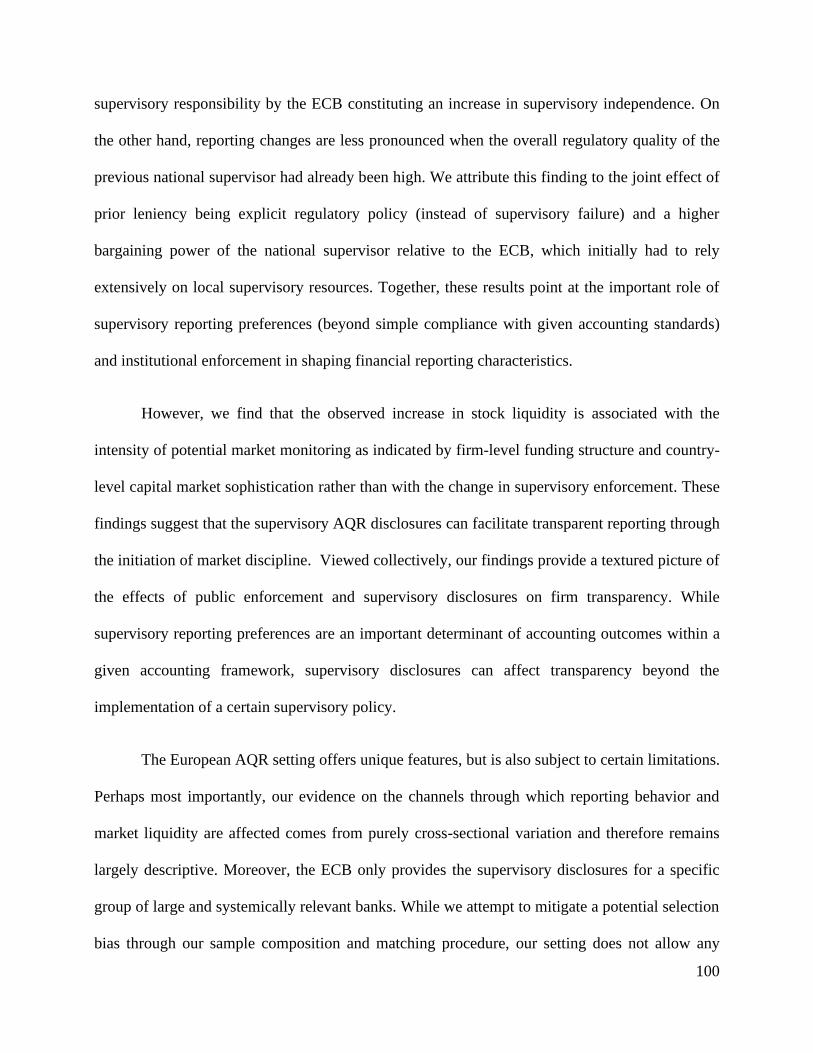
100
supervisory responsibility by the ECB constituting an increase in supervisory independence. On
the other hand, reporting changes are less pronounced when the overall regulatory quality of the
previous national supervisor had already been high. We attribute this finding to the joint effect of
prior leniency being explicit regulatory policy (instead of supervisory failure) and a higher
bargaining power of the national supervisor relative to the ECB, which initially had to rely
extensively on local supervisory resources. Together, these results point at the important role of
supervisory reporting preferences (beyond simple compliance with given accounting standards)
and institutional enforcement in shaping financial reporting characteristics.
However, we find that the observed increase in stock liquidity is associated with the
intensity of potential market monitoring as indicated by firm-level funding structure and country-
level capital market sophistication rather than with the change in supervisory enforcement. These
findings suggest that the supervisory AQR disclosures can facilitate transparent reporting through
the initiation of market discipline. Viewed collectively, our findings provide a textured picture of
the effects of public enforcement and supervisory disclosures on firm transparency. While
supervisory reporting preferences are an important determinant of accounting outcomes within a
given accounting framework, supervisory disclosures can affect transparency beyond the
implementation of a certain supervisory policy.
The European AQR setting offers unique features, but is also subject to certain limitations.
Perhaps most importantly, our evidence on the channels through which reporting behavior and
market liquidity are affected comes from purely cross-sectional variation and therefore remains
largely descriptive. Moreover, the ECB only provides the supervisory disclosures for a specific
group of large and systemically relevant banks. While we attempt to mitigate a potential selection
bias through our sample composition and matching procedure, our setting does not allow any

101
statements about the generalizability of our results for smaller banks that tend to receive less public
scrutiny. We leave these questions for future research.

102
2.6. Appendix B: Variable definitions
Variable Definition Data Source
Firm-level Variables
Tier 1 Tier 1 capital / total risk-weighted assets S&P Global MI
Size Ln(total assets) S&P Global MI
Cost-to-Income Ratio Operating expenses / operating income S&P Global MI
RoA Pre-provision net income / total assets S&P Global MI
Risk-weighted Assets Risk-weighted assets / total assets S&P Global MI
ΔNPL Non-performing loans / Non-performing loanst-1
Loan loss provisions (LLP) Ratio Loan loss provision / total gross loans S&P Global MI
Loan loss allowance (LLA) Ratio Loan loss allowance / total gross loans S&P Global MI
Non-performing loans (NPL) Ratio Non-performing loans / total gross loans S&P Global MI
Coverage Ratio Loan loss allowance / non-performing loans S&P Global MI
Junk Rating Binary variable that takes the value of ‘1’ for banks with
a S&P rating below BBB- S&P Global MI
Short-term Funding Binary variable that takes the value of ‘1’ for firms with
above median short-term deposit ratio (as of 2013) S&P Global MI
Funding Cost Volatility Binary variable that takes the value of ‘1’ for firms with
above median funding cost volatility between 2011-2013 S&P Global MI
AQR Adjustment AQR adjustment on the loan loss provision (additionally
required loan loss provisions) / loan loss allowance in
2013
ECB &
S&P Global MI
Liquidity Variables
Bid-Ask Spread Monthly median of the quoted spread between the bid
and ask price Datastream
Abs(Abnormal Stock Return) Absolute abnormal monthly stock return Datastream
Market Value Monthly median of daily market value Datastream
Share Turnover Monthly median of daily share turnover Datastream
Return Variability Monthly standard deviation of daily returns Datastream
Country Variables
Distrust EU Binary variable that takes the value of ‘1’ for countries
with below median trust in the ECB as of 2014
Eurobarometer
Survey
Distrust ECB Binary variable that takes the value of ‘1’ for countries
with below median trust in the EU as of 2014
Eurobarometer
Survey
Anti-EU Party Binary variable that takes the value of ‘1’ for countries
with at least one Anti-EU party that is represented in the
European Parliament with at least 5% of the seats within
the country as of 2014
Manifesto Project,
Manual Collection
Recession Binary variable that takes the value of ‘1’ for all countries
with negative GDP growth in the two years before the
SSM introduction (2011 and 2012)
World Bank
GDP Yearly Growth in Gross Domestic Product World Bank
Regulatory Quality Binary variable that takes the value of ‘1’ for countries
with above median regulatory quality over the sample
period from 2011-2017
Kaufmann, Kraay,
and Mastruzzi,
(2011)
Equity Ownership Binary variable that takes the value of ‘1’ for countries
with above median ratio of household equity ownership
(2008-2010)
Christensen,
Maffet and Vollon
(2019)
Listed Firms Binary variable that takes the value of ‘1’ for countries
with above median ratio of listed firms to GDP in 2014 World Bank
103
2.7. Appendix C: Entropy balancing
Dependent Variable:
(2)
LLP Ratio
(4)
LLA Ratio
(6)
Coverage Ratio
(8)
NPL Ratio
Test Variables:
SSM Treated -0.003 0.002 -0.028 0.012*
(0.245) (0.567) (0.426) (0.067)
SSM Treated*AQR 0.013* 0.043** -0.047 0.036**
(0.052) (0.012) (0.741) (0.023)
Control Variables:
ΔNPL 0.077***
(0.003)
Tier 1 -0.000 -0.000 0.003 -0.001
(0.820) (0.329) (0.455) (0.365)
Size 0.010*** -0.007 -0.130 0.020
(0.008) (0.243) (0.125) (0.175)
Cost-to-Income -0.000 0.000 0.001 0.000***
(0.687) (0.557) (0.448) (0.006)
RoA 0.065 0.584*** 1.009 1.312***
(0.399) (0.004) (0.415) (0.000)
GDP -0.001* 0.001** 0.006 -0.000
(0.094) (0.032) (0.162) (0.640)
Risk-weighted Assets 0.000*** 0.000 -0.002 0.001
(0.006) (0.162) (0.179) (0.119)
Fixed Effects Year, Firm Year, Firm Year, Firm Year, Firm
N 4,122 6,085 4,329 4,353
Adj. R2 0.636 0.843 0.835 0.930
Appendix C replicates Table 3 using an entropy balanced sample. We use the entropy balancing approach to reweight
the observations in our sample in a way such that the distribution of values of the control variables in the treatment
group is as similar as possible to the distribution in the control group along the first three moments (mean, variance
and skewness). We include year and firm fixed effects in the regressions, but do not report the coefficients. We
winsorize all variables at the 1% and at the 99% level. The table reports OLS coefficient estimates and (in parentheses)
p-values based on robust standard errors clustered by bank. ***, **, and * indicate statistical significance at the 1%,
5%, and 10% levels (two-tailed), respectively.

104
Chapter 3
Legal Efficiency and Non-Performing Loans along the Economic Cycle
“Going into the next downturn with such a high stock of NPLs is simply not an option. And NPLs
are not just concentrated in one or two European countries; they are spread across a number of
countries and a high number of banks. NPLs remain a European issue, no matter where the banks
holding them are located.”
Danièle Nouy, 23/11/2018, in a speech to the European Banking Federation
3.1. Introduction
The global financial crisis and the recent economic fallout due to the corona virus focused
a spotlight on the resilience of banks’ balance sheets and in particular banks’ non-performing loans
(NPLs). If a bank’s borrower gets into arrears, e.g. during economic downturns, the loan is
recorded as non-performing27 resulting in a higher risk-weight28. In addition, the bank might be
required to book a provision against the potential loan loss that impairs net income and regulatory
capital. As a consequence, banks cannot utilize their capital for productive lending and face higher
funding costs due to higher risk-weights. This has severe economic consequences, as high NPL-
levels can impair bank stability (Berger and DeYoung, 1997; Whalen, 1991) and hamstring bank
lending and ultimately economic activity (Barseghyan, 2010). Therefore, a quick work-out of
banks’ non-performing loans, in particular after economic downturns, is key to foster lending and
maintain bank stability.
27 Typically, banks are required to record a loan as non-performing if the borrower is 90-days past due, and the
borrower is unlikely to pay the obligation back in full (ECB, 2017). 28 Under Basel 3, NPLs are subject to a risk weight of 150 percent when applying the standardized approach.
105
After the great financial crisis and the sovereign debt crisis total NPLs in the Eurozone
increased up to 958 billion Euro in December 2014. While NPLs declined to 688 billion Euro in
March 2018, the level of NPLs is still much higher than before the great financial crisis although
most European countries were in an economic growth phase (ECB, 2019). Therefore, regulators
and supervisors continuously highlight the importance of NPLs and made NPL resolution a top
priority in the recent years (e.g., IMF, 2015; ECB, 2016, 2017; ECOFIN, 2017). However, in order
to determine an adequate policy response, it is first necessary to understand the intertemporal and
cross-country determinants of NPLs in the first place.
The existing evidence on the determinants of NPLs consistently documents a negative
correlation between economic growth and NPLs (e.g., Ghosh, 2015; Salas and Saurina, 2002).
Taking these studies at face value one would expect that NPLs are countercyclical to
macroeconomic conditions. That is, NPLs increase in economic downturns and decrease in
economic expansions. In contrast to this assumption, I observe that while all countries in Europe
during the great financial crisis build up NPLs, some countries build up relatively persistent NPL
stocks even within the following expansionary phases. Therefore, it seems unlikely that economic
growth uniformly determines NPLs over the whole business cycle.
There are two non-mutually explanations for this phenomenon. First, it could be that bank-
specific factors, such as profitability, regulatory capital or size are the main enablers of swift NPL
resolution while macroeconomic factors mainly determine how NPL levels build up. Second, the
resolution of NPLs could be shaped by country-specific but not growth-related factors such as legal
efficiency. The conjecture that determinants of NPLs change across business cycles is further
supported by anecdotal evidence from Hoshi and Kashyap (2010) who document that the nature of
NPLs in Japan changed significantly over the economic cycle.

106
Along these lines, policymaker and regulators recognize that a successful NPL resolution
strategy will include insolvency and judicial frameworks that allow cost and time efficient NPL
work-outs (e.g., ECOFIN, 2017; ECB, 2016). Although countries might have similar rules for
contract enforcement and insolvencies, the enforcement of these rules might still depend on the
efficiency of the legal system, such as the speed and honesty of the courts. In particular, collateral
enforcement rules and judicial system inefficiencies, such as weak corporate and household
insolvency frameworks that lead to slow collateral recovery represent a major risk for creditors and
are a notable challenge to NPL resolution (ECB, 2016).
The effect of legal efficiency on NPLs is twofold. First, efficient debt enforcement and
insolvency procedures can ex ante deter loan defaults by changing the borrower’s willingness to
pay. Second, borrowers often secure loans with collateral. If this collateral cannot be realized by
the bank due to lengthy and expensive foreclosure procedures this deters NPL resolution and limits
new bank lending (Haselmann, Pistor, Vig, 2010). Against this backdrop, policymakers should
carefully consider the recent initiatives made during the pandemic, such as the temporary
suspension of the obligation to file for insolvency (§15a InsO) in Germany until the end of October
2020. This suspension could lead to an accumulation of insolvency filings after the end of the
grace period swamping the courts.
Even in normal times, the speed and the costs of insolvency and contract enforcement
procedures vary significantly across countries (Djankov La Porta, Lopez-de-Silanes and Shleifer,
2003). Only a few countries in Europe (e.g., Slovenia and Spain) have efficient and simple out-of-
court insolvency and enforcement mechanisms in place. Furthermore, I expect that the influence
of legal efficiency is likely not uniform over the NPL cycle. While legal efficiency is unlikely to
mitigate increased loan defaults and the building up of NPL stock during economic recessions, it
107
potentially contributes significantly to a fast NPL recovery process in the subsequent periods when
economic growth picks up. Therefore, I make the following two empirical predictions:
Prediction 1: Countries with high legal efficiency can reduce their NPLs earlier compared to
countries with low legal efficiency from the beginning of an economic upturn
Prediction 2: High legal efficiency has an incremental negative association with NPLs during
economic upturns, whereas macroeconomic and bank-specific factors mainly
explain NPLs during economic downturns.
I employ a sample from 17 different European countries to explore these questions using
two sets of analyses. First, I exploit the variation in the duration of NPL cycles across countries to
explore whether legal efficiency and economic growth determine the duration of NPL cycles.
Therefore, I test in a proportional hazard model whether (a) legal efficiency is associated with the
duration of the increasing NPL phase and (b) legal efficiency correlates with the duration until
NPLs decrease from the start of an economic upturn. My findings indicate that while the duration
of an increasing NPL phase is mainly associated with economic growth, the duration towards a
NPL resolution from the beginning of an economic upturn is highly correlated with the efficiency
of the legal procedures in place for contract enforcement and insolvencies.
To test the second prediction, and to benchmark cross-country differences in legal
efficiency with firm factors, I move to the firm-level for the subsequent analyses. Using firm-level
data on NPLs, I document that legal efficiency is highly correlated with NPLs even when
controlling for several firm-level factors, such as profitability, regulatory capital and cost
efficiency. Exploiting variation in economic cycles across countries, I further find legal efficiency
to be negatively associated with NPLs in economic upturns. I confirm that this correlation is mainly

108
confined to the duration and the costs of insolvency and contract enforcement procedures and
cannot be explained by firm factors or other cross-country differences, such as supervisory power
or overall regulatory quality.
I contribute to the existing literature along three dimensions. First, I acknowledge that
associations with NPLs may change over the economic cycle. That is, factors that matter for NPLs
during the increasing NPL phase might not be less relevant during the reduction phase of NPLs
and vice versa. Although there is anecdotal evidence that the nature of NPLs can change over time
(Hoshi and Kashyap, 2010), this is, to the best of my knowledge, the first paper that distinguishes
between different economic and NPL cycles. Second, I contribute to the literature on the
determinants of NPLs (e.g., Barth, Caprio, and Levine, 2004; Gosh, 2015) by exploring bank- and
country-specific factors that potentially explain NPLs in Europe. Third, I add to the literature on
the effects of cross-country differences in the institutional set-up (Djankov et al., 2003; Djankov,
Hart, McLiesh, and Shleifer, 2008) by investigating whether insolvency and contract enforcement
correlate with NPLs along the economic cycle.
The remainder of the paper proceeds as follows. In Section 2, I provide a survey of the
literature on NPLs. Section 3 outlines the research design and describes the sample selection. In
Section 4, I present the results of the cox proportional hazard analysis on the country level and the
regression analysis on the firm level to explore the duration of NPL cycles. Section 5 concludes.

109
3.2. Literature review
The literature on the determinants of non-performing loans can be broadly categorized into
studies that explore (i) country-specific (mostly macroeconomic) and, (ii) bank-specific factors.
An overarching pattern across studies of macroeconomic determinants NPLs is the documented
negative relationship between GDP growth and NPLs (e.g., Ghosh, 2015; Salas and Saurina, 2003;
Cerulli et al., 2019; Breuer, 2006; Beck, Jakubik and Piloiu, 2013). Other macroeconomic
determinants are, inter alia, exchange rates (Klein, 2013; Beck et al., 2013), foreign lending
(Kauko, 2012), share prices (Beck et al., 2013), lending interest rates (Espinoza and Prasad, 2011,
Louzis et al., 2011), unemployment (Ghosh, 2015; Nkusu, 2011), and house prices (Bofondi and
Ropele, 2011; Ghosh, 2015). However, evidence on most associations between NPLs and macro
determinants is not fully conclusive, potentially due to the limited comparability of samples (both
in terms of countries and time periods) and multicollinearity issues when adding highly correlated
macroeconomic growth indicators such as GDP, house prices and unemployment to multivariate
models. Nevertheless, an overarching conclusion from most above mentioned studies is that
economic growth in different facets (GDP, employment, house prices) seems to be negatively
correlated with NPL levels. However, none of the above mentioned studies distinguishes explicitly
between different periods of the business or NPL cycle.
Furthermore, the majority of the literature on NPL determinants focuses on individual
countries, such as the US (Ghosh, 2015), Spain (e.g., Salas and Saurina, 2002), Italy (Bofondi and
Ropele, 2011; Cucinelli, 2015; Japelli et al., 2005) Japan (Mamatzakis, Matousek and Vu, 2015),
India (Ghosh, 2007), Greece (Louzis et al., 2011), the Czech Republic (Podpiera and Weill, 2008),
Romania (Filip, 2014) or specific regions such as the Gulf area (Espinoza and Prasad, 2011), and
eastern Europe (Klein, 2013; Agoraki, 2011) limiting comparability and generalizability.

110
In addition, there is evidence on the role of regulation and disclosure requirements for
NPLs. Barth et al. (2004) find a weakly significant negative association between private
monitoring, strict capital requirement regulations and NPLs. Similar results are documented by
Agoraki et al. (2011) for supervisory power, and Breuer (2006) for off-balance sheet disclosures.
In addition, D’Apice and Fiordelisi (2020) explore the effects of four enforcement reforms between
2008 and 2011 on banks NPLs. In addition, the theoretical model from Japelli, Pagano and Bianco
(2005) shows that assuming and endogenous default rate, judicial efficiency helps to decrease the
average default rate by fostering borrower selection ex ante. Further descriptive evidence from a
sample of Italian districts between 1984 and 1998 indicates that the length of the contract
enforcement process and the backlog of cases at regional courts in Italy are correlated with NPLs.
In addition to cross-country differences, several studies find bank-specific factors to be
correlated with NPLs. Against this backdrop, Berger and DeYoung (1997) document that
decreases in cost efficiency are reflected in higher NPLs due to excess expenditures for the
monitoring of bad loans that, however, on average come along with overall worse monitoring and
underwriting practices. Furthermore, their findings indicate the presence of moral hazard
incentives for weakly capitalized banks that respond to asset quality deteriorations with an increase
in risk-taking. Furthermore, Behr et al. (2009) and Salas and Saurina (2002) document a negative
correlation between bank size and NPLs potentially resulting from better diversification
opportunities. Profitability is also frequently associated with lower NPLs for instance in Greece.
(Louzis et al., 2011) or in Spain (Salas and Saurina, 2002).
Overall then, several studies document that country specific and bank-specific factors
matter for NPLs, however there is a lack of evidence on the association between legal efficiency
and NPLs over the business cycle in Europe.

111
3.3. Research design and data
I evaluate the development of NPLs from two perspectives. First, I use aggregated data on
NPLs within 17 Eurozone countries from the World Bank Global Financial Development Database.
This database includes NPL ratios from the yearly Global Financial Stability Report published by
the International Monetary Fund. I include all Eurozone countries with available information on
macroeconomic growth and legal efficiency measures.
Second, I also analyze annual bank-level information from S&P Global Market Intelligence
(formerly SNL Financial). In contrast to most prior research on NPLs in Europe, I build on a
dataset that includes actual NPLs and not impaired loans (e.g., as provided by Bankscope).
Although, impaired loans are potentially a valid proxy of NPLs, they reflect an accounting concept
(e.g., IAS 39 during my sample period) with substantial discretion (e.g. Ryan and Liu, 2006)
compared to NPLs which are a supervisory construct (Regulation (EU) No 680/2014).
Furthermore, while the ECB definition of NPLs includes all loans that are 90-days past due and the
debtor is unlikely-to-pay (ECB 2017), the accounting definition (IAS 39) of impaired loans requires
a dedicated ‘trigger event’ indicating that the loan will not be repaid in full. As a consequence, the
definition of NPLs is much broader than the concept of impaired loans. Therefore, relying on
impaired loans as a proxy for NPLs can lead to wrong conclusions if specific reporting incentives
are embedded in the reporting of impaired loans.
The final firm-level sample includes all banks that have available data on the macro-level
variables (GDP and legal efficiency) and information on bank-level control variables (tier 1
regulatory capital, total assets, loans, cost-to-income, return on assets). The sample period for both
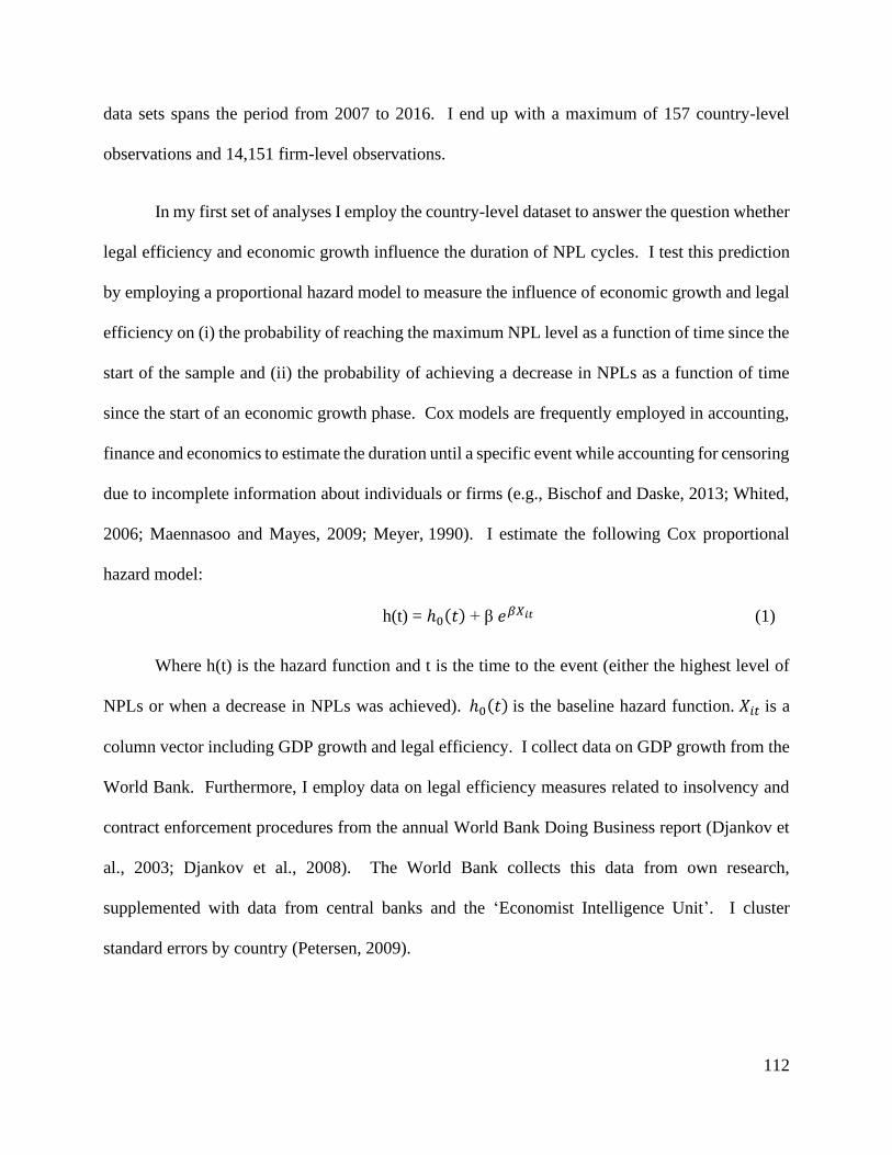
112
data sets spans the period from 2007 to 2016. I end up with a maximum of 157 country-level
observations and 14,151 firm-level observations.
In my first set of analyses I employ the country-level dataset to answer the question whether
legal efficiency and economic growth influence the duration of NPL cycles. I test this prediction
by employing a proportional hazard model to measure the influence of economic growth and legal
efficiency on (i) the probability of reaching the maximum NPL level as a function of time since the
start of the sample and (ii) the probability of achieving a decrease in NPLs as a function of time
since the start of an economic growth phase. Cox models are frequently employed in accounting,
finance and economics to estimate the duration until a specific event while accounting for censoring
due to incomplete information about individuals or firms (e.g., Bischof and Daske, 2013; Whited,
2006; Maennasoo and Mayes, 2009; Meyer, 1990). I estimate the following Cox proportional
hazard model:
h(t) = ℎ0(𝑡) + β 𝑒𝛽𝑋𝑖𝑡 (1)
Where h(t) is the hazard function and t is the time to the event (either the highest level of
NPLs or when a decrease in NPLs was achieved). ℎ0(𝑡) is the baseline hazard function. 𝑋𝑖𝑡 is a
column vector including GDP growth and legal efficiency. I collect data on GDP growth from the
World Bank. Furthermore, I employ data on legal efficiency measures related to insolvency and
contract enforcement procedures from the annual World Bank Doing Business report (Djankov et
al., 2003; Djankov et al., 2008). The World Bank collects this data from own research,
supplemented with data from central banks and the ‘Economist Intelligence Unit’. I cluster
standard errors by country (Petersen, 2009).

113
In the second set of analyses, I employ bank-level data from S&P Global Market
Intelligence to explore whether macroeconomic, bank-specific or cross-country differences in legal
efficiency are associated with NPLs over the economic cycles. I start with an estimation of the
following fixed effect OLS model over the sample period from 2006 to 2016:
NPL Ratio = β0 + β1 Legal Efficiency + β2 GDP + β3 Recovery + β4 Legal Efficiency * Recovery
+ β5 GDP * Recovery + ∑ βi Controls + ∑ βj Fixed Effects + ε (1)
The dependent variable NPL Ratio is the percentage of non-performing loans divided by
gross loans. There are four main variables of interest. GDP as the annual gross domestic product
growth rate in the respective country obtained from the World Bank and Legal Efficiency that
stands for a vector of binary partitioning variables that capture systematic variation in legal
efficiency with respect to contract enforcement and insolvency procedures. Furthermore, I explore
whether GDP and Legal Efficiency have diverging effects over the economic cycle by interacting
both variables with Recovery that stands for a binary variable that takes the value of ‘1’ beginning
from the first year a country enters an economic growth phase that lasts at least 3 years after 2009.29
I use two sets of proxies for Legal Efficiency. First, I use individual binary splits for
countries that have above median Insolvency Durations, Insolvency Costs, Insolvency Recovery
Rates, Contract Enforcement Durations, Contract Enforcement Costs, and Contract Enforcement
Scores. Second, I sum up all binary insolvency and contract enforcement measures (excluding
only the enforcement score that itself captures a summary measure already) to build a composite
Legal Efficiency Score. In addition, I employ a binary partitioning variable that takes the value of
‘1’ for countries with an above median Legal Efficiency Score (LE) that I label High Legal
29 I use three consecutive economic growth years as proxy for a recovery to avoid misclassifying countries as
“recovering” that were affected by the sovereign debt crisis in 2011/12 shortly after the great financial crisis.

114
Efficiency (High LE). The base effect of these split variables is time-invariant and therefore
subsumed by the firm fixed effect. Controls denotes the following firm-level control variables:
Size as the natural logarithm of total assets, RoA as the percentage of pre-provisioning income to
total assets as a measure of banks’ profitability, Tier 1 as the percentage of banks’ tier 1 capital to
risk-weighted assets, Cost-Income as the percentage of operating expense to operating income
measuring banks’ efficiency. Loan Ratio as the ratio of total gross loans to total assets. I include
year- and firm-fixed effects, which account for the general time trend as well as time-invariant
bank and country characteristics (e.g., the overall quality of the legal system or the development of
capital markets). As such, my fixed-effects structure subsumes factors that are specific to a certain
year or a particular bank. In all my tests, I draw statistical inferences based on standard errors
clustered by country to adjust for correlation between banks within countries and time-series
correlation within countries (Petersen, 2009).
I rely on a fixed effect model to deal with unobserved heterogeneity and omitted variables
instead of a dynamic panel model with the lagged dependent variable as the I am particularly
interested in the correlations between NPLs that build up with relative persistence during an
economic downturn and decrease during an economic downturn. Nevertheless, I follow the
approach from Ghosh (2015) and confirm that my inference is robust within a dynamic panel
system-GMM estimation including lagged NPLs as explanatory variable (Arellano and Bover,
1995; Blundell and Bond, 1998).30
30 Furthermore, as the fixed effect estimator brackets the true effect (Guyan, 2001), I follow the recommendation
from Angrist and Pischke (2008) and rely on a fixed effect model for my analyses.

115
3.4. Empirical results
3.4.1. Descriptive statistics
I start with a descriptive analysis of NPLs across countries. Figure 3.1 plots the yearly NPL
ratios of countries with high and low legal efficiency. The figure illustrates that on average
countries follow a similar NPL growth trajectory until 2013 regardless of their legal efficiency.
However, countries with high legal efficiency reach their highest NPL level in 2013, while still
rising for countries with low legal efficiency.
Figure 3.1 NPL Ratios and GDP Development for High vs. Low Legal Efficiency Countries
Figure 3.1 shows the NPL Ratios development over the sample period from 2007-2016 for high and low legal
efficiency countries. NPL Ratios are normalized to zero in 2013.

116
An obvious concern from this descriptive observation is that the NPL development could
be simply a reflection of different economic growth patterns across countries that I capture with
the legal efficiency measure. However, when depicting GDP growth by legal efficiency in
Figure 3.2, I document relatively similar average economic growth patterns across these two sets
of countries. From this descriptive analyses, I conclude that while both high and low legal
efficiency countries follow similar patterns during the buildup phase of the NPL cycle that is likely
determined by economic developments, countries that achieve significant reductions in NPLs are
characterized by efficient insolvency and enforcement procedures that come into play during
economic growth periods.
Figure 3.1. GDP Development for High vs. Low Legal Efficiency Countries
Figure 3.2 shows the GDP growth development over the sample period from 2007-2016 for high and low legal
efficiency countries. GDP growth is normalized to zero in 2013.

117
I explore this conjecture in the next section with a more formal analysis. Additional
descriptive statistics in Table 3.1, Panel A confirm that the average NPL ratio varies greatly across
countries. The NPL ratio varies between 0.4% in Luxembourg and 27% in Cyprus. Table 1, Panel
B shows pairwise correlations between NPLs and GDP and legal efficiency measures. Legal
efficiency and in particular the enforcement duration is highly positively correlated with NPLs.

118
Ta
ble
3.1
Des
crip
tiv
e st
ati
stic
s a
nd
pa
irw
ise
corr
ela
tio
ns
on
th
e co
un
try
lev
el
Pa
nel
A D
escr
ipti
ve S
tati
stic
s
Co
un
try
Co
un
try
-Yea
rs
Mea
n N
PL
Rat
io
Mea
n G
DP
M
ean
LE
H
igh
LE
En
forc
emen
t
Du
rati
on
Inso
lven
cy
Du
rati
on
Au
stri
a 1
0
2.7
17
1.0
26
3.0
00
1.0
00
1.1
03
1.1
00
Bel
giu
m
10
3.1
37
1.1
09
3.7
00
1.0
00
1.4
03
0.8
90
Cy
pru
s 8
2
7.3
31
-0.4
36
2.6
25
1.0
00
2.2
95
1.5
00
Est
on
ia
9
2.6
56
0.2
87
1.0
00
0.0
00
1.1
81
3.0
00
Fra
nce
9
3
.94
0
0.5
84
2.0
00
1.0
00
1.0
17
1.9
00
Ger
man
y
10
2.6
69
1.3
06
4.5
00
1.0
00
1.1
33
1.2
00
Gre
ece
9
21
.896
-3
.287
1.0
00
0.0
00
3.1
28
2.6
67
Irel
and
10
14
.141
4
.21
4
1.9
00
0.0
00
1.6
56
0.4
00
Ital
y
10
12
.678
-0
.542
1.0
00
0.0
00
3.2
97
1.8
00
Lat
via
9
8
.26
6
-0.2
23
1.5
56
0.0
00
1.1
15
2.1
67
Lit
hu
ania
9
1
2.8
26
1
.19
3
2.2
22
1.0
00
0.7
96
1.8
33
Lu
xem
bo
urg
6
0
.42
7
1.5
72
2.0
00
0.0
00
0.8
92
2.0
00
Mal
ta
10
6.8
50
4.0
03
0.0
00
0.0
00
1.4
03
3.0
00
Net
her
lan
ds
9
2.7
76
0.6
27
3.0
00
1.0
00
1.4
28
1.1
00
Po
rtu
gal
1
0
9.1
31
-0.1
04
1.8
00
0.0
00
1.5
36
2.0
00
Slo
ven
ia
9
9.4
77
0.2
19
2.3
33
1.0
00
3.5
09
1.7
33
Sp
ain
1
0
5.5
62
0.3
78
2.5
00
1.0
00
1.4
24
1.3
00
Pa
nel
B P
air
wis
e C
orr
ela
tio
ns
N
PL
G
DP
H
igh
LE
L
E
Inso
lven
cy
Du
rati
on
En
forc
emen
t
Du
rati
on
NP
L R
atio
1
.00
00
GD
P
-0.0
94
3
1.0
000
Hig
h L
E
-0.1
37
4
-0.0
08
8
1.0
000
LE
-
0.2
320
*
-0.0
10
8
0.6
890
*
1.0
000
Inso
lven
cy D
ura
tio
n
0.1
538
-0.1
42
0
-0.4
46
5*
-0.6
47
9*
1.0
000
En
forc
emen
t D
ura
tion
0
.51
61
*
-0.0
97
5
-0.1
74
2
-0.2
72
2*
0.1
666
1.0
000
Tab
le 3
.1 P
anel
A s
ho
ws
des
crip
tiv
e st
atis
tics
fo
r al
l co
un
try
-lev
el v
aria
ble
s u
sed
in o
ur
cou
ntr
y-l
evel
tes
ts.
Pan
el B
sh
ow
s p
airw
ise
corr
elat
ion
s fo
r th
e
cou
ntr
y-l
evel
var
iab
les.
* i
nd
icat
e st
atis
tica
l si
gn
ific
ance
at
the
5%
lev
el.
All
var
iab
les
are
def
ined
in A
pp
end
ix D
.
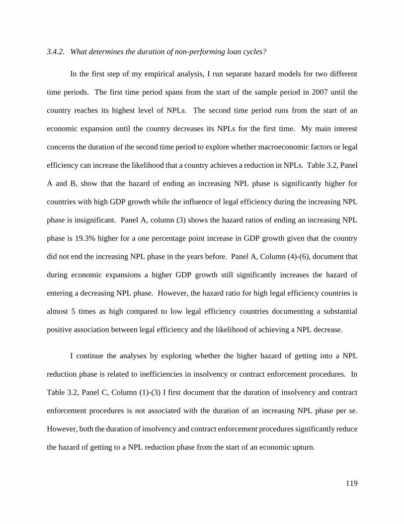
119
3.4.2. What determines the duration of non-performing loan cycles?
In the first step of my empirical analysis, I run separate hazard models for two different
time periods. The first time period spans from the start of the sample period in 2007 until the
country reaches its highest level of NPLs. The second time period runs from the start of an
economic expansion until the country decreases its NPLs for the first time. My main interest
concerns the duration of the second time period to explore whether macroeconomic factors or legal
efficiency can increase the likelihood that a country achieves a reduction in NPLs. Table 3.2, Panel
A and B, show that the hazard of ending an increasing NPL phase is significantly higher for
countries with high GDP growth while the influence of legal efficiency during the increasing NPL
phase is insignificant. Panel A, column (3) shows the hazard ratios of ending an increasing NPL
phase is 19.3% higher for a one percentage point increase in GDP growth given that the country
did not end the increasing NPL phase in the years before. Panel A, Column (4)-(6), document that
during economic expansions a higher GDP growth still significantly increases the hazard of
entering a decreasing NPL phase. However, the hazard ratio for high legal efficiency countries is
almost 5 times as high compared to low legal efficiency countries documenting a substantial
positive association between legal efficiency and the likelihood of achieving a NPL decrease.
I continue the analyses by exploring whether the higher hazard of getting into a NPL
reduction phase is related to inefficiencies in insolvency or contract enforcement procedures. In
Table 3.2, Panel C, Column (1)-(3) I first document that the duration of insolvency and contract
enforcement procedures is not associated with the duration of an increasing NPL phase per se.
However, both the duration of insolvency and contract enforcement procedures significantly reduce
the hazard of getting to a NPL reduction phase from the start of an economic upturn.

120
Table 3.2 Influence of legal efficiency and GDP on the duration of NPL cycles
Panel A: Hazard Ratios for Legal Efficiency and GDP
Duration of NPL Increase Duration until NPL decrease in Recovery
(1) (2) (3) (4) (5) (6)
High LE 1.687 2.190 4.544** 4.985**
(0.303) (0.132) (0.035) (0.026)
GDP 1.142** 1.193*** 1.158* 1.198**
(0.018) (0.001) (0.067) (0.012)
N 133 133 133 26 26 26
Panel B: Hazard Ratios for Enforcement Duration, Insolvency Duration, and GDP
Duration of NPL Increase Duration until NPL decrease in Recovery
(1) (2) (3) (4) (5) (6) Insolvency Duration 0.988 1.023 0.716 0.602**
(0.947) (0.907) (0.374) (0.021)
Enforcement Duration 0.876 0.872 0.178*** 0.132***
(0.617) (0.623) (0.005) (0.003)
GDP 1.143** 1.128** 1.126** 1.180 1.104 1.102*
(0.011) (0.025) (0.019) (0.109) (0.107) (0.061)
N 126 126 126 25 25 25
Table 3.2 shows results from cox proportional hazard models reporting the effect of legal efficiency and economic
growth on the duration of the two different phases of the NPL cycle. High LE is a binary variable that takes the value of
‘1’ if the country is above the median legal efficiency of all countries in that year. GDP is the yearly GDP growth. All
other variables are defined in Appendix D. We winsorize all variables at the 1% and at the 99% level. The table reports
hazard ratios and (in parentheses) p-values based on robust standard errors clustered by country. ***, **, and * indicate
statistical significance at the 1%, 5%, and 10% levels (two-tailed), respectively.

121
Taken together, the country-level analysis provides first indications that legal efficiency
measures are significantly associated with the duration until NPLs decrease from the start of an
upturn, while economic growth determines how NPLs build up during recessions. In order to
benchmark these findings against the influence of bank-specific factors, I continue in the next step
with an analysis on the bank level.
3.4.3. Country-level factors versus bank-specific determinants of NPLs
I start the bank-level analysis with a correlation analysis in Table 3.3. Panel B shows that
NPLs are negatively correlated with legal efficiency, GDP, profitability, and tier 1 capital while
positively correlated with size, the loan ratio, and the cost-income ratio. I explore these correlations
more formally estimating the fixed effect OLS regression from model (2) in, Table 3.4. Column (1)
indicates that banks in high legal efficiency countries have on average 1.68% lower NPL ratios
compared to banks in low legal efficiency countries (p-value<0.01). Furthermore, in Column (4),
I document that the negative association of legal efficiency is solely confined to expansion periods.
The coefficient on High LE*Recovery documents that banks in high legal efficiency countries have
on average a 6.6% lower NPL ratio (p-value<0.02) during economic upturns compared to low legal
efficiency countries. In addition, I find that during economic recovery periods banks have on
average 2.5% higher NPL ratios (p-value<0.03). The coefficient signs on my control variables
show positive correlations between profitability, loan ratios, cost-income ratios31, tier 1 ratios and
NPL ratios.
31 This result is in favor of the bad luck hypothesis from Berger and DeYoung (1998). Under the bad luck hypothesis
increases in problem loans are caused by exogenous events such as an economic downturn and subsequently
require extra expenses for managing these exposures. Therefore, the additional expenses for NPL management
create an impression of higher cost-to-income ratios (and hence, lower cost efficiency) for banks that put
substantial effort in the resolution of NPLs.

122
Ta
ble
3.3
Des
crip
tiv
e st
ati
stic
s o
n t
he
ba
nk
lev
el
Pa
nel
A D
escr
ipti
ve S
tati
stic
s
Co
un
try
Ban
ks
Ban
k-
Yea
rs
Mea
n
Siz
e
Mea
n.
Lo
an R
atio
Mea
n
Co
st-I
nco
me
Mea
n
Tie
r 1
Mea
n
Ro
A
Mea
n
NP
L
Au
stri
a 4
3
24
8
19
.201
0
.58
5
67
.731
10
.276
0.4
21
8.7
87
Bel
giu
m
11
87
19
.317
0
.53
2
54
.975
15
.994
0.7
19
3.3
35
Est
on
ia
5
35
11
.037
0
.40
8
21
9.5
02
14
.132
-5.6
90
8.2
28
Fin
lan
d
75
48
7
10
.274
0
.78
8
72
.852
65
.493
0.7
66
0.9
37
Fra
nce
8
5
51
8
18
.312
0
.46
7
47
.071
18
.287
0.0
36
3.5
60
Ger
man
y
15
62
81
87
14
.419
0
.54
6
70
.308
18
.390
0.1
33
3.5
52
Gre
ece
12
80
17
.724
0
.66
7
45
.694
10
.198
1.1
13
20
.750
Irel
and
16
86
16
.499
1.0
40
39
.084
12
.232
-5.8
98
14
.106
Ital
y
55
8
34
67
12
.887
0
.57
3
68
.214
14
.316
0.0
99
13
.732
Lat
via
7
2
1
15
.500
0
.58
9
39
.182
40
.167
2.2
42
8.8
91
Lit
hu
ania
6
2
6
14
.343
0
.56
2
48
.412
12
.122
1.4
05
19
.264
Lu
xem
bo
urg
1
4
84
16
.337
0
.19
5
81
.420
13
.652
0.5
41
5.3
71
Mal
ta
12
74
14
.146
0
.00
0
37
.923
36
.830
1.0
77
9.7
22
Net
her
lan
ds
24
14
3
17
.167
0
.63
0
66
.667
16
.215
0.2
35
5.2
83
Po
rtu
gal
3
8
19
1
11
.880
0
.48
4
64
.036
27
.638
-0.0
94
7.7
69
Slo
ven
ia
9
60
15
.571
0
.71
2
53
.974
8.6
32
0.2
23
17
.992
Sp
ain
6
7
35
7
13
.390
0.0
23
65
.579
61
.373
0.6
31
6.4
65
Pa
nel
B P
air
wis
e C
orr
ela
tio
ns
N
PL
Rat
io
Siz
e L
oan
Rat
io
Co
st-I
nco
me
Tie
r 1
Ro
A
GD
P
Hig
h L
E
Rec
ov
ery
NP
L R
atio
1
.00
00
Siz
e 0
.02
49
*
1.0
000
Lo
an R
atio
0
.04
07
*
0.0
009
1.0
000
Co
st-I
nco
me
0.0
116
-0.1
62
5*
-0.0
27
4*
1
.00
00
Tie
r 1
-0.0
42
3*
-0.1
36
9*
-0.1
09
1*
0
.07
85
*
1.0
000
Ro
A
-0.2
15
5*
0.0
029
-0.0
31
6*
-0.3
06
4*
0.0
250
*
1.0
000
GD
P
-0.2
26
3*
-0.0
48
4*
-0.0
17
6
0.0
274
*
-0.0
25
4*
0.0
839
*
1.0
000
Hig
h L
E
-0.5
66
5*
-0.1
22
3*
-0.0
16
6
0.0
389
*
-0.0
60
4*
0.0
358
*
0.3
338
*
1.0
000
Rec
ov
ery
-0.2
75
7*
-0.1
34
7*
-0.0
51
2*
0
.05
88
*
-0.0
14
8
0.0
222
*
0.3
442
*
0.5
249
*
1.0
000
Tab
le 3
.3 P
anel
A s
ho
ws
des
crip
tiv
e st
atis
tics
fo
r al
l fi
rm-l
evel
var
iab
les
use
d i
n o
ur
ban
k-l
evel
tes
ts.
Pan
el B
sh
ow
s p
airw
ise
corr
elat
ion
s fo
r th
e b
ank-
lev
el a
nd
cou
ntr
y-l
evel
var
iab
les.
* i
nd
icat
e st
atis
tica
l si
gn
ific
ance
at
the
5%
lev
el.
All
var
iab
les
are
def
ined
in
Ap
pen
dix
D.

123
Table 3.4 Legal Efficiency along the economic cycle and NPL ratios
Dependent Variable:
(1)
NPL Ratio
(2)
NPL Ratio
(3)
NPL Ratio
(4)
NPL Ratio
Test Variables:
High LE -1.681*** -0.955 2.285
(0.002) (0.209) (0.134)
GDP 0.547 0.526 0.362**
(0.127) (0.152) (0.032)
Recovery 2.562**
(0.021)
High LE * Recovery -6.634**
(0.015)
GDP * Recovery -0.045
(0.773)
Control Variables:
Size -0.065 0.221 0.181 -0.248
(0.875) (0.569) (0.656) (0.623)
Loan Ratio -0.393* -0.380* -0.375* -0.319**
(0.065) (0.056) (0.054) (0.019)
Cost-Income -0.016** -0.018*** -0.018*** -0.014**
(0.011) (0.008) (0.008) (0.015)
Tier 1 -0.053** -0.047* -0.047* -0.039
(0.045) (0.057) (0.054) (0.111)
RoA -0.537* -0.584* -0.582* -0.521*
(0.068) (0.054) (0.054) (0.064)
Constant 5.856 -0.914 0.288 5.621
(0.241) (0.848) (0.958) (0.382)
Fixed Effects Year, Firm Year, Firm Year, Firm Year, Firm
SE Clustered by Country Country Country Country
Observations 14,151 14,151 14,151 14,151
R-squared 0.129 0.150 0.151 0.249
Adjusted R-squared 0.128 0.149 0.150 0.248
Table 3.4 shows regression results for the effect of legal efficiency, economic growth and bank-specific factors on
the level of banks’ non-performing loans ratio. High LE is a binary variable that takes the value of ‘1’ if the country
is above the median legal efficiency of all countries in that year. GDP is the yearly GDP growth. Recovery is a binary
variable that takes the value of ‘1’ beginning in the first year that the country enters a period of three years consecutive
GDP growth. All other variables are defined in Appendix D. We include year and firm fixed effects in the regressions,
but do not report the coefficients. We winsorize all variables at the 1% and at the 99% level. The table reports OLS
coefficient estimates and (in parentheses) p-values based on robust standard errors clustered by country. ***, **, and
* indicate statistical significance at the 1%, 5%, and 10% levels (two-tailed), respectively.

124
3.4.4. The role of contract enforcement and insolvency proceedings for NPLs
I continue with a closer examination of the association between legal efficiency and NPL
ratios. In particular, I study the role of insolvency and contract enforcement procedures for NPL
ratios over the economic cycle. For these additional cross-sectional tests, I replace the legal
efficiency indicator variable in Equation (2) with six different binary partitioning variables that
measure the efficiency of insolvency resolution and contract enforcement. Table 3.5, Column
(1)-(3) show that Insolvency Duration, Insolvency Costs, and Insolvency Recovery Rate are
significantly associated with NPLs in recovery. Column (1) and (2) document that in expansionary
periods an above median insolvency duration or above median insolvency costs are associated with
NPL ratios that are on average approximately 7% higher compared to below median countries in
recovery periods (p-value<0.02). In addition, I find that banks in countries with a high Insolvency
Recovery Rate experience on average 6.6% lower NPL ratios relative to banks in countries with
low recovery rates during economic recoveries.
I find corroborating results when looking at the three different contract enforcement
measures. Table 3.5, Column (4)-(6) document that above median Enforcement Duration and
Enforcement Costs are significantly positive associated with NPL ratios during economic upturns.
Furthermore, banks in countries with overall better contract enforcement, and therefore, with a
higher contract Enforcement Score experience on average 9% lower NPL ratios in economic
upturns (p-value<0.01).
Overall, my results confirm the hypothesis that insolvency and contract enforcement
procedures are significantly associated with NPLs on the country and on the bank level.
Furthermore, I document that this association is confined to economic recovery periods.

125
Ta
ble
3.5
Co
ntr
act
en
forc
emen
t, i
nso
lven
cy p
roce
du
res
an
d N
PL
ra
tio
s
In
solv
ency
Pro
cedu
res
En
forc
emen
t P
roce
du
res
NP
L R
ati
o a
s D
epen
den
t V
ari
ab
le
(1)
Inso
lven
cy
Du
rati
on
(2)
Inso
lven
cy
Co
sts
(3)
Inso
lven
cy
Rec
ove
ry R
ate
(4)
En
forc
emen
t
Du
rati
on
(5)
En
forc
emen
t
Co
sts
(6)
En
forc
emen
t
Sco
re
Tes
t V
ari
ab
les:
Sp
lit*
Rec
ov
ery
6.8
41
**
7.2
88
***
-6
.645
**
1
0.0
33
***
7
.14
9***
-9
.010
***
(0.0
17
) (0
.009
) (0
.017
) (0
.000
) (0
.005
) (0
.000
)
Rec
ov
ery
-4.4
91
**
-4
.519
**
2
.46
0**
-6.3
64
***
-4
.266
**
3
.39
9***
(0.0
19
) (0
.013
) (0
.029
) (0
.000
) (0
.015
) (0
.000
)
GD
P *
Rec
ov
ery
0.0
38
-0.0
11
0
.01
3
0.1
73
0
.00
9
0.1
40
(0
.851
) (0
.955
) (0
.950
) (0
.236
) (0
.962
) (0
.413
)
GD
P
0.4
47
***
0
.37
7**
0
.47
1***
0
.08
3
0.3
94
**
0.1
66
*
(0.0
08
) (0
.018
) (0
.007
) (0
.491
) (0
.038
) (0
.093
)
Co
ntr
ol
Var
iab
les
Yes
Y
es
Yes
Y
es
Yes
Y
es
Fix
ed E
ffec
ts
Yea
r, F
irm
Y
ear,
Fir
m
Yea
r, F
irm
Y
ear,
Fir
m
Yea
r, F
irm
Y
ear,
Fir
m
SE
Clu
ster
ed b
y
Co
un
try
Co
un
try
Co
un
try
Co
un
try
C
ou
ntr
y
Co
un
try
N
13
,664
13
,664
1
3,6
64
13
,664
13
,664
13
,664
R2
0.2
52
0.2
59
0
.25
1
0.3
18
0
.26
3
0.2
92
Ad
j. R
2
0.2
51
0.2
58
0
.25
0
0.3
17
0
.26
2
0.2
91
Tab
le 5
sho
ws
reg
ress
ion
res
ult
s fo
r th
e ef
fect
of
inso
lven
cy p
roce
du
res,
co
ntr
act
enfo
rcem
ent
pro
ced
ure
s, e
cono
mic
gro
wth
an
d b
ank
-sp
ecif
ic f
acto
rs o
n t
he
lev
el o
f b
ank
s’ n
on
-per
form
ing
lo
ans
rati
o.
Inso
lven
cy D
ura
tio
n,
Inso
lven
cy C
ost
s, I
nso
lven
cy R
eco
very
Ra
te,
En
forc
emen
t D
ura
tio
n,
En
forc
emen
t C
ost
s a
nd
En
forc
emen
t S
core
are
bin
ary v
aria
ble
s th
at t
ake
the
val
ue
of
‘1’
if t
he
cou
ntr
y i
s ab
ov
e th
e m
edia
n f
or
the
resp
ecti
ve
spli
t v
aria
ble
of
all
co
un
trie
s du
rin
g t
he
sam
ple
per
iod
fro
m 2
007
-20
16
. H
igh
er v
alu
es f
or
En
forc
emen
t S
core
in
dic
ate
bet
ter
con
trac
t en
forc
emen
t pro
cedu
res.
GD
P is
the
yea
rly
GD
P g
row
th. R
eco
very
is a
bin
ary
var
iab
le t
hat
tak
es t
he
val
ue
of
‘1’
beg
inn
ing i
n t
he
firs
t y
ear
that
th
e co
un
try
en
ters
a p
erio
d o
f th
ree
yea
rs c
on
secu
tiv
e G
DP
gro
wth
. A
ll o
ther
var
iab
les
are
def
ined
in
Ap
pen
dix
D.
We
incl
ud
e y
ear
and
fir
m f
ixed
eff
ects
in
th
e re
gre
ssio
ns,
bu
t do
no
t re
port
th
e co
effi
cien
ts.
We
win
sori
ze a
ll v
aria
ble
s at
the
1%
an
d a
t th
e 9
9%
lev
el.
Th
e ta
ble
rep
ort
s O
LS
co
effi
cien
t es
tim
ates
an
d (
in p
aren
thes
es)
p-v
alu
es b
ased
on
rob
ust
sta
nd
ard
err
ors
clu
ster
ed b
y c
ou
ntr
y.
**
*,
**,
and
* i
nd
icat
e st
atis
tica
l si
gn
ific
ance
at
the
1%
, 5
%,
and
10
% l
evel
s (t
wo
-tai
led
), r
esp
ecti
vel
y.

126
3.4.5. Robustness tests
In the last step, I perform three robustness tests that replicate Table 4 with different sets of
additional control variables. In Table 3.6, Column (1), I additionally interact all control variables
with the binary Recovery variable to test whether the association between the bank-level control
variables and NPLs changes over the business cycle. I confirm the inference from Table 3.4,
although the coefficient on High LE*Recovery is slightly lower (6.58 vs. -6.6, p-value<0.05).
In the next step, I address concerns that NPL ratios that might also serve as a supervisory
measure of financial stability are driven by supervisory power or general regulatory quality rather
than legal efficiency. In Column (2), I employ additional controls for supervisory power, private
monitoring, external governance and the requirement for external audit from Barth, Caprio,
Levine (2013). My inference remains qualitatively and quantitatively robust. The main coefficient
of interest Legal Efficiency * Recovery is significant at the 5% level although the effect size is
slightly lower (-4.3 vs. -6.6, p-value<0.05). However, I do not document a significant association
between the proxies for supervisory power and NPLs.
In Column (3), I alternatively employ additional control variables from the World Bank’s
Worldwide Governance Indicators (WGI) database to proxy for institutional differences and the
strength of the legal system (Kaufmann, Kraay, and Mastruzzi, 2011). I proxy for six different
constructs in this analysis: Political stability, voice and accountability, regulatory quality, rule of
law, control of corruption and government effectiveness. I continue to find a significant negative
association between Legal Efficiency * Recovery and the NPL ratio although the effect size is again
slightly lower (-5.2 vs. -6.6, p-value<0.05).

127
Overall, I show that the incremental association between legal efficiency and NPLs in
economic upturns remains robust even when controlling for proxies of supervisory power, overall
regulatory quality and political stability. Future research can explore these additional covariates in
more detail.

128
Table 3.6 Robustness tests with additional controls
Dependent Variable
(4)
NPL Ratio
(4)
NPL Ratio
(4)
NPL Ratio
Test Variables:
High LE 2.377 1.533 -0.245
(0.139) (0.417) (0.839)
GDP 0.393** 0.495** -0.209
(0.022) (0.011) (0.137)
Recovery 4.443** 2.791*** 1.502
(0.048) (0.006) (0.259)
High LE * Recovery -6.584** -4.334** -5.260**
(0.013) (0.036) (0.015)
GDP * Recovery -0.058 -0.124 0.400*
(0.713) (0.632) (0.074)
Control Variables:
Size -0.301 -0.347 -0.860
(0.494) (0.492) (0.162)
Loan Ratio -0.822 -0.306** -0.231***
(0.175) (0.018) (0.000)
Cost-Income -0.024*** -0.014*** -0.003
(0.001) (0.003) (0.420)
Tier 1 -0.026 -0.044* -0.038
(0.102) (0.060) (0.126)
RoA -0.624*** -0.502* -0.433*
-0.246 (0.090) (0.079)
Constant -0.301 -9.908 57.519***
(0.494) (0.186) (0.001)
Additional Controls Controls*Recovery
Bank Regulation
and Supervision
Governance and
Institutional
Differences
Fixed Effects Year, Firm Year, Firm Year, Firm
SE Clustered by Country Country Country
Observations 14,151 14,151 14,151
R-squared 0.258 0.366 0.366
Adjusted R-squared 0.256 0.365 0.365
Table 3.6 replicates Table 4 using additional control variables for the general regulatory and legal environment, and
supervisory power. Column (1) includes an interaction between Recovery and all control variables (Size, Loan Ratio,
Cost-Income, Tier 1, RoA). Column (2) adds five different proxies for the regulatory and supervisory environment from
Barth, Caprio, and Levine (2013): Supervisory Power, Private Monitoring, External Audit, and External Governance.
Column (3) adds six different proxies for the general institutional environment from Kaufmann, Kraay, and Mastruzzi
(2011): Corruption, Government Effectiveness, Political Stability and Absence of Violence, Rule of Law, Regulatory
Quality, Voice and Accountability. High LE is a binary variable that takes the value of ‘1’ if the country is above the
median legal efficiency of all countries in that year. GDP is the yearly GDP growth. Recovery is a binary variable that
takes the value of ‘1’ beginning in the first year that the country enters a period of three years consecutive GDP growth.
All other variables are defined in Appendix D. We include year and firm fixed effects in the regressions, but do not
report the coefficients. We winsorize all variables at the 1% and at the 99% level. The table reports OLS coefficient
estimates and (in parentheses) p-values based on robust standard errors clustered by country. ***, **, and * indicate
statistical significance at the 1%, 5%, and 10% levels (two-tailed), respectively.

129
3.5. Conclusion
This paper has analyzed the determinants of NPLs from a new angle, one that explores the
difference of macroeconomic, country-specific and bank-specific correlations with NPLs along the
business cycle. Using country-level data on NPLs, I find that the time period from the start of an
economic upturn until a reduction in NPLs occurs, is significantly shorter for countries with high
legal efficiency. In addition, if insolvency and contract enforcement procedures are inefficient,
this reduces the likelihood to get into a phase of decreasing NPLs even under favorable
macroeconomic conditions.
I corroborate these findings with a bank-level analysis benchmarking differences in legal
efficiency against other determinants of NPLs, such as GDP growth, regulatory capital,
profitability, and cost efficiency. Similar to the evidence on the aggregate level, I find that banks
in countries with high legal efficiency have on average incrementally lower NPLs during economic
upturns. That is, my results suggest that the association of legal efficiency with NPLs changes over
the business cycle. Further analyses reveal that these effects are robust for several proxies of legal
efficiency. Furthermore, I provide evidence that the association of legal efficiency with NPLs is
not confined to supervisory quality or the general regulatory quality within the country.
Finally, the findings can help to inform regulators, policymakers and supervisors when
addressing high NPL levels in the future. This seems of particular relevance due to the recent
pandemic-driven economic downturn that will likely result in NPL increases during the subsequent
periods. However, my results back up the view that bank regulators and supervisors may only have
parts of the toolkit that is needed to foster a swift NPL resolution process after economic downturns.

130
3.6. Appendix D: Variable definitions
Variable Definition / Description Data Source
Firm-level Variables
TIER 1 (Tier 1 capital / total risk-weighted assets)*100 Capital IQ MI
Size Ln(total assets) Capital IQ MI
Loan Ratio Total gross loans/ total assets Capital IQ MI
Cost-Income (Operating expenses / operating income)*100 Capital IQ MI
RoA (Pre-provision net income / total assets)*100 Capital IQ MI
NPL Ratio (Non-performing loans / total gross loans)*100 Capital IQ MI
Country Variables
GDP Yearly % growth in gross domestic product World Bank
NPL Ratio (Non-performing loans / total gross loans)*100 World Bank
Legal Efficiency (LE) Summary Measure: Number of measures for which a
country is below the median of all sample countries:
Insolvency duration. Enforcement duration,
insolvency cost, enforcement costs, insolvency
recovery rate.
Djankov et al. (2003);
Djankov et al., (2008)
Insolvency Duration Above Median Average Duration for Insolvency
Procedures
Djankov et al., (2008)
Enforcement. Duration Above Median Average Days for Contract
Enforcement Procedures
Djankov et al. (2003)
Insolvency Costs Above Median Average Costs for Insolvency
Procedures
Djankov et al., (2008)
Enforcement Costs Above Median Average Costs for Contract
Enforcement Procedures
Djankov et al. (2003)
Insolvency. Rec. Rate Above Median Recovery Rate in Insolvencies Djankov et al., (2008)
Enforcement. Score Above Median Contract Enforcement Score Djankov et al. (2003)
Supervisory Power Whether the supervisory authorities have the
authority to take specific actions to prevent and
correct problems
Barth, Caprio, and
Levine (2013)
Private Monitoring Measures whether there incentives/ability for the
private monitoring of firms, with higher values
indicating more private monitoring
Barth, Caprio, and
Levine (2013)
External Audit The effectiveness of external audits of banks
Barth, Caprio, and
Levine (2013)
External Governance Higher values indicate better corporate governance
(audit, accounting, financial statement transparency,
external ratings and credit monitoring)
Barth, Caprio, and
Levine (2013)
Corruption Control of corruption captures perceptions of the
extent to which public power is exercised for private
gain, including both petty and grand forms of
corruption, as well as "capture" of the state by elites
and private interests.
Kaufmann, Kraay,
and Mastruzzi (2011)
Government Effectiveness Government effectiveness captures perceptions of
the quality of public services, the quality of the civil
service and the degree of its independence from
political pressures, the quality of policy formulation
and implementation, and the credibility of the
government's commitment to such policies.
Kaufmann, Kraay,
and Mastruzzi (2011)
Political Stability and
Absence of Violence
Political Stability and Absence of
Violence/Terrorism measures perceptions of the
likelihood of political instability and/or politically
motivated
violence, including terrorism.
Kaufmann, Kraay,
and Mastruzzi (2011)

131
3.6 Appendix D (continued)
Variable Definition / Description Data Source
Rule of Law Rule of law captures perceptions of the extent to
which agents have confidence in and abide by the
rules of society, and in particular the
quality of contract enforcement, property rights, the
police, and the courts, as well as the likelihood of
crime and violence.
Kaufmann, Kraay,
and Mastruzzi (2011)
Regulatory Quality Regulatory quality captures perceptions of the ability
of the government to formulate and implement sound
policies and regulations that
permit and promote private sector development.
Kaufmann, Kraay,
and Mastruzzi (2011)
Voice and Accountability Voice and accountability captures perceptions of the
extent to which a country's citizens are able to
participate in selecting their government, as well as
freedom of expression, freedom of association, and a
free media.
Kaufmann, Kraay,
and Mastruzzi (2011)

132
Concluding Remarks
This thesis presents three essays on financial reporting incentives and bank transparency. While
the first study documents the importance of manager incentives and preferences for banks’
accounting choices, the second and the third study explore firm- and country-specific incentives
that matter for banks’ accounting and reporting behavior.
Chapter 1 investigates the role of individual managers in the financial reporting of banks.
Exploiting the connectedness between different managers as well as a set of plausibly exogenous
manager turnovers, we find that managerial idiosyncrasies explain approximately 19% of banks’
discretionary loan loss provisions. We identify common patterns in bank managers’ reporting
behavior over time that point at general differences in the idiosyncratic influence across managers.
Using these differences to construct bank manager profiles, we document how the role of individual
manager types interacts with top management team composition. Overall, divergence in the
revealed preferences of the top management team for different accounting and policy choices
significantly confines the idiosyncratic manager influence on banks’ loan loss provisioning
Chapter 2 investigates how supervisors influence bank transparency through supervisory
disclosures and public enforcement. Upon adoption of the Single Supervisory Mechanism (SSM)
for major Eurozone banks, the European Central Bank (ECB) as the new supervisor undertook a
comprehensive review of bank balance sheets and publicly disclosed the results of this Asset
Quality Review (AQR). The AQR disclosures revealed what the ECB perceived to be a substantial
overvaluation of bank assets, and in particular problem loans. The magnitude of the AQR
adjustments varied substantially across supervised banks. We exploit this firm-level variation as
well as the staggered introduction of the SSM to analyze the change in affected banks’ reporting
behavior and transparency. The ECB’s preference for more conservative reporting is associated

133
with higher levels of loan loss provisions and non-performing loan classifications in the following
periods. Pointing at the role of enforcement institutions, this reporting effect is particularly
pronounced for firms whose prior national supervisors were more likely to be captured by political
interest. At the same time, corresponding positive liquidity effects are concentrated among SSM
banks that were exposed to potential pressure from market forces. Our findings suggest that
supervisory disclosures are potentially effective in establishing greater transparency of the banking
sector, but depend on the presence of firm-level incentives that help establish market discipline.
Finally, in Chapter 3, I investigate the role of legal efficiency for banks’ non-performing loans
along the business cycle in 17 European countries. During the global financial crisis and the
subsequent sovereign debt crisis all European countries experienced a substantial increase in NPLs.
I find that increases in NPLs are mainly associated with macroeconomic and bank-specific
determinants. However, I recognize that substantial differences in the duration and efficiency of
the NPL resolution after the crisis exist. I exploit cross-country differences in insolvency and
contract enforcement procedures to document that non-performing loans are associated with the
duration and the costs of insolvency and contract enforcement during economic growth phases. My
findings suggest that the duration of the decreasing NPL phase depends on the presence of an
efficient insolvency and contract enforcement regime that ensures swift non-performing loan
resolution while the duration of increasing NPL phases is mainly determined by economic
conditions.

134
References
Abowd, J. M., Kramarz, F., Margolis, D. N., Abowd, B. Y. J. M., Kramarz, F., & Margolis, D. N.
(1999). High Wage Workers and High Wage Firms, Econometrica, 67(2), 251-333.
Abowd, J. M., Creecy, R. H., & Kramarz, F. (2002). Computing person and firm effects using
linked longitudinal employer-employee data, Center for Economic Studies, (No. 2002-06),
US Census Bureau.
Acharya, V. V., & Ryan, S. G. (2016). Banks’ financial reporting and financial system stability.
Journal of Accounting Research, 54(2), 277-340.
Acharya, V. V., & Steffen, S. (2014). Making sense of the comprehensive assessment. SAFE
Policy Letter, Research Report No. 32. Retrieved from
https://www.econstor.eu/handle/10419/106982
Adams, R., & Ferreira, D. (2010). Moderation in groups: Evidence from betting on ice break-ups
in Alaska. The Review of Economic Studies, 77(3), 882-913.
Adams, R., Keloharju, M., & Knüpfer, S. (2018). Are CEOs born leaders? Lessons from traits of a
million individuals. Journal of Financial Economics, 130(2), 392-408.
Agarwal, S., Amromin, G., Ben‐David, I., & Dinc, S. (2018). The Politics of Foreclosures. The
Journal of Finance, 73(6), 2677-2717.
Agarwal, S., Lucca, D., Seru, A., & Trebbi, F. (2014). Inconsistent regulators: Evidence from
banking. The Quarterly Journal of Economics, 129(2), 889-938.
Agoraki, M. E. K., Delis, M. D., & Pasiouras, F. (2011). Regulations, competition and bank risk-
taking in transition countries. Journal of Financial Stability, 7(1), 38-48.
Ahmed, A. S., Takeda, C., & Thomas, S. (1999). Bank loan loss provisions: a reexamination of
capital management, earnings management and signaling effects. Journal of Accounting and
Economics, 28(1), 1-25.
Ahmed, A. S., Christensen, B. E., Olson, A. J., & Yust, C. G. (2019). Déjà vu: The effect of
executives and directors with prior banking crisis experience on bank outcomes around the
global financial crisis. Contemporary Accounting Research, 36(2), 958-998.
Albuquerque, A. M., De Franco, G., & Verdi, R. S. (2013). Peer choice in CEO
compensation. Journal of Financial Economics, 108(1), 160-181.
Ali, A., & Zhang, W. (2015). CEO tenure and earnings management. Journal of Accounting and
Economics, 59(1), 60-79.
Andrews, M. J., Gill, L., Schank, T., & Upward, R. (2008). High wage workers and low wage
firms: negative assortative matching or limited mobility bias? Journal of the Royal Statistical
Society: Series A (Statistics in Society), 171(3), 673-697.
Angrist, J. D., & Pischke, J. S. (2008). Mostly harmless econometrics: An empiricist's companion.
NJ: Princeton University Press.
Arellano, M., & Bover, O. (1995). Another look at the instrumental variable estimation of error-
components models. Journal of Econometrics, 68(1), 29-51.

135
Armstrong, C. S., Guay, W. R., & Weber, J. P. (2010). The role of information and financial
reporting in corporate governance and debt contracting. Journal of Accounting and
Economics, 50(2-3), 179-234.
Armstrong, C. S., Larcker, D. F., Ormazabal, G., & Taylor, D. J. (2013). The relation between
equity incentives and misreporting: The role of risk-taking incentives. Journal of Financial
Economics, 109(2), 327-350.
Baik, B. O. K., Farber, D. B., & Lee, S. A. M. (2011). CEO ability and management earnings
forecasts. Contemporary Accounting Research, 28(5), 1645-1668.
Bamber, L. S., Jiang, J., & Wang, I. Y. (2010). What’s my style? The influence of top managers
on voluntary corporate financial disclosure. The Accounting Review, 85(4), 1131-1162.
Bantel, K. A., & Jackson, S. E. (1989). Top management and innovations in banking: Does the
composition of the top team make a difference? Strategic Management Journal, 10(S1), 107-
124.
Barseghyan, L. (2010). Non-performing loans, prospective bailouts, and Japan's
slowdown. Journal of Monetary Economics, 57(7), 873-890.
Barth, J. R., Caprio Jr, G., & Levine, R. (2004). Bank regulation and supervision: what works
best? Journal of Financial Intermediation, 13, 205-248.
Barth, J. R., Caprio, G., & Levine, R. (2013). Bank regulation and supervision in 180 countries
from 1999 to 2011. Journal of Financial Economic Policy. 5(2), 111-219.
Barth, M. E., & Landsman, W. R. (2010). How did financial reporting contribute to the financial
crisis?. European Accounting Review, 19(3), 399-423.
Beatty, A. L., Ke, B., & Petroni, K. R. (2002). Earnings management to avoid earnings declines
across publicly and privately held banks. The Accounting Review, 77(3), 547-570.
Beatty, A., & Liao, S. (2014). Financial accounting in the banking industry: A review of the
empirical literature. Journal of Accounting and Economics, 58(2-3), 339-383.
Beaver, W., Eger, C., Ryan, S., & Wolfson, M. (1989). Financial reporting, supplemental
disclosures, and bank share prices. Journal of Accounting Research, 27(2), 157-178.
Behr, P., Schmidt, R. H., & Xie, R. (2010). Market structure, capital regulation and bank risk
taking. Journal of Financial Services Research, 37(2-3), 131-158.
Berger, A. N., & De Young, R. (1997). Problem loans and cost efficiency in commercial
banking. Journal of Banking & Finance, 21, 849-870.
Beck, R., Jakubik, P., & Piloiu, A. (2013). Non-performing loans: What matters in addition to the
economic cycle? Working Paper. Retrieved from
https://papers.ssrn.com/sol3/papers.cfm?abstract_id=2214971
Beck, P.J. & Narayanamoorthy, G.S., (2013). Did the SEC impact banks’ loan loss reserve policies
and their informativeness? Journal of Accounting and Economics, 56(2-3), pp.42-65.
Beltratti, A., & Stulz, R. M. (2012). The credit crisis around the globe: Why did some banks
perform better? Journal of Financial Economics, 105(1), 1-17.

136
Berger, A. N., Kick, T., & Schaeck, K. (2014). Executive board composition and bank risk taking.
Journal of Corporate Finance, 28, 48-65.
Berger, A. N., Davies, S. M., & Flannery, M. J. (2000). Comparing market and supervisory
assessments of bank performance: who knows what when? Journal of Money, Credit and
Banking, 32(3), 641-667.
Berger, A. N., & Turk-Ariss, R. (2015). Do Depositors Discipline Banks and Did Government
Actions During the Recent Crisis Reduce this Discipline? An International
Perspective. Journal of Financial Services Research, 48(2), 103-126.
Bertrand, M., & Schoar, A. (2003). Managing with style: The effect of managers on firm policies.
The Quarterly Journal of Economics, 118(4), 1169-1208.
Bhat, G., Ryan, S. G., & Vyas, D. (2018). The Implications of Credit Risk Modeling for Banks’
Loan Loss Provisions and Loan-Origination Procyclicality. Management Science, 65(5),
2116-2141.
Bischof, J., & Daske, H. (2013). Mandatory Disclosure, Voluntary Disclosure, and Stock Market
Liquidity: Evidence from the EU Bank Stress Tests. Journal of Accounting Research, 51(5),
997-1029.
Bischof, J., Daske, H., Elfers, F., & Hail, L. (2020). A tale of two supervisors: Compliance with
risk disclosure regulation in the banking sector. Working Paper. Retrieved from
https://papers.ssrn.com/sol3/papers.cfm?abstract_id=2580569
Blundell, R., & Bond, S. (1998). Initial conditions and moment restrictions in dynamic panel data
models. Journal of Econometrics, 87(1), 115-143.
Bofondi, M., & Ropele, T. (2011). Macroeconomic determinants of bad loans: evidence from
Italian banks. Bank of Italy Occasional Paper, (89). Retrieved from
https://papers.ssrn.com/sol3/papers.cfm?abstract_id=1849872
Breuer, J. B. (2006). Problem bank loans, conflicts of interest, and institutions. Journal of
Financial Stability, 2(3), 266-285.
Brochet, F., Miller, G. S., Naranjo, P., & Yu, G. (2019). Managers' cultural background and
disclosure attributes. The Accounting Review, 94(3), 57-86.
Busch, D., & Teubner, A. (2019). Fit and Proper Assessments within the Single Supervisory
Mechanism. European Banking Institute Working Paper Series 2019, No. 34, Retrieved from
https://papers.ssrn.com/sol3/papers.cfm?abstract_id=3346976
Bushman, R. M. (2014). Thoughts on financial accounting and the banking industry. Journal of
Accounting and Economics, 58(2-3), 384-395.
Bushman, R. M., & Williams, C. D. (2012). Accounting discretion, loan loss provisioning, and
discipline of Banks’ risk-taking. Journal of Accounting and Economics, 54(1), 1-18.
Bushman, R. M., & Williams, C. D. (2015). Delayed expected loss recognition and the risk profile
of banks. Journal of Accounting Research, 53(3), 511-553.
Bushman, R. M. (2016). Transparency, accounting discretion, and bank stability. Economic Policy
Review, August, 129-149.

137
Bushman, R. M., Davidson, R. H., Dey, A., & Smith, A. (2018). Bank CEO materialism: Risk
controls, culture and tail risk. Journal of Accounting and Economics, 65(1), 191-220
Busuioc, E. M. (2016). Friend or foe? Inter‐agency cooperation, organizational reputation, and
turf. Public Administration, 94(1), 40-56.
Caliński, T., & Harabasz, J. (1974). A dendrite method for cluster analysis. Communications in
Statistics-Theory and Methods, 3(1), 1-27.
Calomiris C. W. & Kahn C. M. (1991) The role of demandable debt in structuring optimal banking
arrangements. American Economic Review, 81, 497-513.
Campbell, T. C., Gallmeyer, M., Johnson, S. A., Rutherford, J., & Stanley, B. W. (2011). CEO
optimism and forced turnover. Journal of Financial Economics, 101(3), 695-712.
Carboni, M., Fiordelisi, F., Ricci, O., & Lopes, F. S. S. (2017). Surprised or not surprised? The
investors’ reaction to the comprehensive assessment preceding the launch of the banking
union. Journal of Banking & Finance, 74(Supplement C), 122-132.
Cerulli,G., D’Apice, V., Fiordelisi, F., Masala, F. (2019). Benchmarking Non-Performing Loans.
Working Paper. Retrieved from
https://papers.ssrn.com/sol3/papers.cfm?abstract_id=2903851
Chapman, K. L., Miller, G. S., & White, H. D. (2019). Investor relations and information
assimilation. The Accounting Review, 94(2), 105-131.
Chen, Y., & Hasan, I. (2006). The transparency of the banking system and the efficiency of
information-based bank runs. Journal of Financial Intermediation, 15(3), 307-331.
Choi, W., Han, S., Jung, S. H., & Kang, T. (2015). CEO's operating ability and the association
between accruals and future cash flows. Journal of Business Finance & Accounting, 42(5-6),
619-634.
Christensen, D. M., Jones, K. L., & Kenchington, D. G. (2018). Gambling attitudes and financial
misreporting. Contemporary Accounting Research, 35(3), 1229-1261.
Christensen, H. B., Hail, L., & Leuz, C. (2013). Mandatory IFRS reporting and changes in
enforcement. Journal of Accounting and Economics, 56(2-3), 147-177.
Christensen, H. B., Maffett, M., & Vollon, L. (2019). Securities regulation, household equity
ownership, and trust in the stock market. Review of Accounting Studies, 24(3), 824-859.
Coles, J. L., Daniel, N. D., & Naveen, L. (2006). Managerial incentives and risk-taking. Journal of
Financial Economics, 79(2), 431-468.
Collins, J. H., Shackelford, D. A., & Wahlen, J. M. (1995). Bank differences in the coordination of
regulatory capital, earnings, and taxes. Journal of Accounting Research, 33(2), 263-291.
Core, J., & Guay, W. (2002). Estimating the value of employee stock option portfolios and their
sensitivities to price and volatility. Journal of Accounting Research, 40(3), 613-630.
Costello, A. M., Granja, J., & Weber, J. (2019). Do Strict Regulators Increase the Transparency of
Banks? Journal of Accounting Research, 57(3), 603-637.

138
Crossland, C., & Hambrick, D. C. (2007). How national systems differ in their constraints on
corporate executives: A study of CEO effects in three countries. Strategic Management
Journal, 28(8), 767-789.
Curry, T.J. (2013). Remarks before the AICPA Banking Conference, September 16, 2013.
Retrieved from https://www.occ.treas.gov/news-issuances/speeches/2013/pub-speech-2013-
136.pdf
Custodio, C., & Metzger, D. (2014). Financial expert CEOs: CEO׳ s work experience and firm׳ s
financial policies. Journal of Financial Economics, 114(1), 125-154.
D'Apice, V., & Fiordelisi, F. (2020). Judicial Efficiency and Lending Quality. Working Paper.
Retrieved from https://papers.ssrn.com/sol3/papers.cfm?abstract_id=3557159
Davidson, R., Dey, A., & Smith, A. (2015). Executives’ “off-the-job” behavior, corporate culture,
and financial reporting risk. Journal of Financial Economics, 117(1), 5-28.
Davidson, R. H., Dey, A., & Smith, A. J. (2019). CEO materialism and corporate social
responsibility. The Accounting Review, 94(1), 101-126.
Davis, A. K., Ge, W., Matsumoto, D., & Zhang, J. L. (2015). The effect of manager-specific
optimism on the tone of earnings conference calls. Review of Accounting Studies, 20(2), 639-
673.
Dejong, D., & Ling, Z. (2013). Managers: Their effects on accruals and firm policies. Journal of
Business Finance & Accounting, 40(1-2), 82-114.
Demerjian, P. R., Lev, B., Lewis, M. F., & McVay, S. E. (2013). Managerial ability and earnings
quality. Accounting Review, 88(2), 463-498.
Demirgüç-Kunt, A., & Huizinga, H. (2010). Bank activity and funding strategies: The impact on
risk and returns. Journal of Financial Economics, 98(3), 626-650.
Dessein, W., & Santos, T. (2020) Managerial Style and Attention. American Economic Journal:
Microeconomics, forthcoming.
Diamond, D. W., & Verrecchia, R. E. (1991). Disclosure, liquidity, and the cost of capital. The
Journal of Finance, 46(4), 1325-1359.
DiMaggio, P. J., & Powell, W. W. (1983). The iron cage revisited: institutional isomorphism and
collective rationality in organizational fields. American Sociological Review, 48(2), 147-160.
Dimitrios, A., Helen, L., & Mike, T. (2016). Determinants of non-performing loans: Evidence from
Euro-area countries. Finance Research Letters, 18, 116-119.
Djankov, S., La Porta, R., Lopez-de-Silanes, F., & Shleifer, A. (2003). Courts. The Quarterly
Journal of Economics, 118(2), 453-517.
Djankov, S., Hart, O., McLiesh, C., & Shleifer, A. (2008). Debt enforcement around the
world. Journal of Political Economy, 116(6), 1105-1149.
Dudley, W. (2009). Some lessons from the crisis. Remarks at the Institute of International Banks
Membership Luncheon, New York City.

139
Dugan, J. C (2009). Loan Loss Provisioning and Pro-cyclicality. Remarks before the Institute of
International Bankers, March 2, 2009. Retrieved from
https://www.occ.gov/news-issuances/speeches/2009/pub-speech-2009-16.pdf
Duro, M., Heese, J., & Ormazabal, G. (2019). The effect of enforcement transparency: Evidence
from SEC comment-letter reviews. Review of Accounting Studies, 24(3), 780-823.
Dyreng, S. D., Hanlon, M., & Maydew, E. L. (2010). The effects of executives on corporate tax
avoidance. Accounting Review, 85(4), 1163-1189.
Dyreng, S. D., Mayew, W. J., & Williams, C. D. (2012). Religious social norms and corporate
financial reporting. Journal of Business Finance & Accounting, 39(7-8), 845-875.
Eber, M., & Minoiu, C. (2017). How Do Banks Adjust to Stricter Supervision? Working Paper.
Retrieved from https://papers.ssrn.com/abstract=2662502
EC (2014). Eurobarometer Survey. European Commission. Retrieved from
https://ec.europa.eu/commfrontoffice/publicopinion/index.cfm
ECB (2014a). Guide to banking supervision. European Central Bank, November 2014. Retrieved
from https://www.bankingsupervision.europa.eu/ecb/pub/pdf/
ssmguidebankingsupervision201411.en.pdf?807838fa2-a8bb958749f411c432d1f3e
ECB (2014b). Aggregate Report on the Comprehensive Assessment. European Central Bank,
October 2014. Retrieved from
https://www.bankingsupervision.europa.eu/ecb/pub/pdf/aggregatereportonthecomprehensiv
eassessmentexsum201410.en.pdf?7e232769b9508e18b653e6dffa1b1f8e
ECB (2016). Stocktake of national supervisory practices and legal frameworks related to NPLs.
European Central Bank. Retrieved from
https://www.bankingsupervision.europa.eu/legalframework/publiccons/pdf/npl/stock_takin
g.en.pdf
ECB (2017). Stocktake of national supervisory practices and legal frameworks related to NPLs.
European Central Bank. Retrieved from
https://www.bankingsupervision.europa.eu/ecb/pub/pdf/ssm.stock_taking2017.en.pdf
ECB (2018a). Guide to fit and proper assessments. Retrieved from
https://www.bankingsupervision.europa.eu/ecb/pub/pdf/ssm.fap_guide_201705_rev_20180
5.en.pdf
ECB (2018b). SSM Supervisory Manual - European banking supervision: functioning of the SSM
and supervisory approach. European Central Bank, March 2018. Retrieved from
https://www.bankingsupervision.europa.eu/ecb/pub/pdf/ssm.supervisorymanual201803.en.
pdf?1584b27046baf-1e68f92f82caadb3a63
ECB (2019). Communication on supervisory coverage expectations for NPEs. European Central
Bank. Retrieved from
https://www.bankingsupervision.europa.eu/press/letterstobanks/shared/pdf/2019/ssm.super
visory_coverage_expectations_for_NPEs_201908.en.pdf
ECOFIN (2017). Non-Performing Loans – Action Plan. European Commission: Council Economic
and Financial Affairs. 3555th Council meeting, Brussels.

140
Edmans, A., Gabaix, X., & Landier, A. (2009). A multiplicative model of optimal CEO incentives
in market equilibrium. The Review of Financial Studies, 22(12), 4881-4917.
Espinoza, R., Prasad, A., & Williams, O. (2011). Regional financial integration in the
GCC. Emerging Markets Review, 12(4), 354-370.
European Court of Auditors (2016). Single Supervisory Mechanism - Good Start, but Further
Improvement Needed. Special Report 29/2016. Retrieved from
https://www.eca.europa.eu/en/Pages/DocItem.aspx?did=39744
Fee, C. E., Hadlock, C. J., & Pierce, J. R. (2013). Managers with and without style: Evidence using
exogenous variation. The Review of Financial Studies, 26(3), 567-601.
Fernandes, M., Igan, D., & Pinheiro, M. (2017). March madness in Wall Street: (What) does the
market learn from stress tests? Journal of Banking & Finance, 112, 105250.
Ferri, F., Zheng, R., & Zou, Y. (2018). Uncertainty about managers’ reporting objectives and
investors’ response to earnings reports: Evidence from the 2006 executive compensation
disclosures. Journal of Accounting and Economics, 66(2-3), 339-365.
Filip, B. F. (2014). Non-performing loans-dimension of the non-quality of bank lending/loans and
their specific connections. Theoretical and Applied Economics, 5(594), 127-146.
Financial Times (2009). Fortis shareholders leave Belgian depositors out cold. Financial Times,
February 12, 2009. Retrieved from https://www.ft.com/content/3926631c-f93e-11dd-90c1-
000077b07658
Financial Times (2010).UK and US call for bank transparency. Financial Times, June 3, 2010.
Retrieved from https://www.ft.com/content/a3122ce0-6ea2-11df-ad16-00144feabdc0
Financial Times (2011). Dexia agrees to Belgian bail-out. Financial Times, October 10, 2011.
Retrieved from
https://www.ft.com/content/af0f7f4e-f307-11e0-8383-00144feab49a
Financial Times (2017). Nordea to move its headquarters to Finland. Financial Times,
September 6, 2017. Retrieved from https://www.ft.com/content/1ed979fe-9318-11e7-a9e6-
11d2f0ebb7f0
Fiordelisi, F., Ricci, O., & Lopes, F. S. S. (2017). The Unintended Consequences of the Launch
of the Single Supervisory Mechanism in Europe. Journal of Financial and Quantitative
Analysis, 52(6), 2809-2836.
Fitch (2019). Basel Foreclosure Proposal May Push EU Insolvency Reform. Retrieved from
https://www.reuters.com/article/idUSFit953307
Flannery, M. J. (1994) Debt maturity and the deadweight cost of leverage: optimally financing
banking firms. American Economic Review, 84, 320-331.
Flannery, M. J. (2001). The Faces of “Market Discipline”. Journal of Financial Services
Research, 20(2-3), 107-119.
Flannery, M., Hirtle, B., & Kovner, A. (2017). Evaluating the information in the federal reserve
stress tests. Journal of Financial Intermediation, 29, 1-18.
Freixas, X., & Laux, C. (2011). Disclosure, transparency, and market discipline. Working Paper.
Retrieved from https://papers.ssrn.com/sol3/papers.cfm?abstract_id=1964321

141
Fremeth, A. R., & Holburn, G. L. F. (2012). Information Asymmetries and Regulatory Decision
Costs: An Analysis of U.S. Electric Utility Rate Changes 1980-2000. Journal of Law,
Economics, and Organization, 28(1), 127-162.
Gallemore, J. (2019). Bank Financial Reporting Opacity and Regulatory Intervention. Working
Paper. Retrieved from https://ssrn.com/abstract=2838541
Garlappi, L., Giammarino, R., & Lazrak, A. (2017). Ambiguity and the corporation: Group
disagreement and underinvestment. Journal of Financial Economics, 125(3), 417-433.
Ge, W., Matsumoto, D., & Zhang, J. L. (2011). Do CFOs have style? An empirical investigation
of the effect of individual CFOs on accounting practices. Contemporary Accounting
Research, 28(4), 1141-1179.
Gebhardt, G. U., & Novotny‐Farkas, Z. (2011). Mandatory IFRS Adoption and Accounting Quality
of European Banks. Journal of Business Finance & Accounting, 38(3‐4), 289-333.
Ghosh, A. (2015). Banking-industry specific and regional economic determinants of non-
performing loans: Evidence from US states. Journal of Financial Stability, 20, 93-104.
Ghosh, S. (2007). Does Financial Liberalization Lower Problem Loans in Banks? Economic
Notes, 36(2), 171-188.
Gipper, B., Leuz, C., & Maffett, M. (2019). Public Oversight and Reporting Credibility: Evidence
from the PCAOB Audit Inspection Regime. The Review of Financial Studies, forthcoming.
Goldstein, I., & Sapra, H. (2014). Should banks' stress test results be disclosed? An analysis of the
costs and benefits. Foundations and Trends in Finance, 8(1), 1-54.
Goldstein, I., & Yang, L. (2019). Good disclosure, bad disclosure. Journal of Financial Economics,
131(1), 118-138.
Gormley, T. A., & Matsa, D. A. (2014). Common errors: How to (and not to) control for
unobserved heterogeneity. The Review of Financial Studies, 27(2), 617-661.
Graham, J. R., Li, S., & Qiu, J. (2012). Managerial attributes and executive compensation. Review
of Financial Studies, 25(1), 144-186.
Graham, J. R., Harvey, C. R., & Puri, M. (2013). Managerial attitudes and corporate actions.
Journal of Financial Economics, 109(1), 103-121.
Granja, J. (2018). Disclosure regulation in the commercial banking industry: Lessons from the
national banking era. Journal of Accounting Research, 56(1), 173-216.
Granja, J., & Leuz, C. (2019). The Death of a Regulator: Strict Supervision, Bank Lending and
Business Activity Retrieved from https://papers.ssrn.com/abstract=3092284
Griffin, P. A., & Wallach, S. J. (1991). Latin American lending by major US banks: The effects of
disclosures about nonaccrual loans and loan loss provisions. Accounting Review, 66(4),
830-846.
Gropp, R., Mosk, T., Ongena, S., & Wix, C. (2019). Banks response to higher capital requirements:
Evidence from a quasi-natural experiment. The Review of Financial Studies, 32(1), 266-299.
Guryan, J. (2001). Does money matter? Regression-discontinuity estimates from education finance
reform in Massachusetts (No. w8269). National Bureau of Economic Research.

142
Hagendorff, J., Collins, M., & Keasey, K. (2010). Board monitoring, regulation, and performance
in the banking industry: Evidence from the market for corporate control. Corporate
Governance: An International Review, 18(5), 381-395.
Hagendorff, J., Saunders, A., Steffen, S., & Vallascas, F. (2018). The Wolves of Wall Street :
Managerial Attributes and Bank Business Models. Working Paper, Retrieved from
https://papers.ssrn.com/Sol3/papers.cfm?abstract_id=2670525
Hainmueller, J. (2012). Entropy balancing for causal effects: A multivariate reweighting method
to produce balanced samples in observational studies. Political Analysis, 20(1), 25-46.
Ham, C., Seybert, N., & Wang, S. (2018). Narcissism is a bad sign: CEO signature size, investment,
and performance. Review of Accounting Studies, 23(1), 234-264.
Hambrick, D. C., & Mason, P. A. (1984). Upper Echelons: The Organization as a Reflection of Its
Top Managers. Academy of Management Review, 9(2), 193-206.
Hambrick, D. C. (2007). Upper echelons theory: An update. Academy of Management Review,
32(2), 334-343.
Hambrick, D. C., & Quigley, T. J. (2014). Toward more accurate contextualization of the CEO
effect on firm performance. Strategic Management Journal, 35(4), 473-491.
Haselmann, R., Pistor, K., & Vig, V. (2010). How law affects lending. The Review of Financial
Studies, 23(2), 549-580.
Herring, R., (2004). How can the invisible hand strengthen prudential supervision? And how can
prudential supervision strengthen the invisible hand? in: Borio, C. et al. (ed.), Market
Discipline Across Countries and Industries, MIT Press, Cambridge, MA.
Hollander, S., & Verriest, A. (2016). Bridging the gap: the design of bank loan contracts and
distance. Journal of Financial Economics, 119(2), 399-419.
Holthausen, R. W. (2009). Accounting Standards, Financial Reporting Outcomes, and
Enforcement. Journal of Accounting Research, 47(2), 447-458.
Homar, T., Kick, H., & Salleo, C. (2015). What Drives Forbearance-Evidence from the ECB
Comprehensive Assessment. Retrieved from
https://papers.ssrn.com/sol3/papers.cfm?abstract_id=2707565
Hoshi, T., & Kashyap, A. K. (2010). Will the US bank recapitalization succeed? Eight lessons from
Japan. Journal of Financial Economics, 97(3), 398-417.
Hribar, P., & Yang, H. (2016). CEO overconfidence and management forecasting. Contemporary
Accounting Research, 33(1), 204-227.
Huang, H. W., Rose-Green, E., & Lee, C. C. (2012). CEO age and financial reporting quality.
Accounting Horizons, 26(4), 725-740.
Huang, J., & Kisgen, D. J. (2013). Gender and corporate finance: Are male executives
overconfident relative to female executives? Journal of Financial Economics, 108(3), 822-
839.
IMF (2015). A Strategy for Resolving Europe’s Problem Loans. IMF Staff Discussion Note
SDN/15/19. Retrieved from https://www.imf.org/external/pubs/ft/sdn/2015/sdn1519.pdf

143
IMF (2018). Euro Area Policies: Financial System Stability Assessment. IMF Staff Country
Report No. 18/226. Retrieved from
https://www.imf.org/en/Publications/CR/Issues/2018/07/19/Euro-Area-Policies-Financial-
System-Stability-Assessment-46100
Jackson, H. E., & Roe, M. J. (2009). Public and private enforcement of securities laws: Resource-
based evidence. Journal of Financial Economics, 93(2), 207-238.
Jappelli, T., Pagano, M., & Bianco, M. (2005). Courts and banks: Effects of judicial enforcement
on credit markets. Journal of Money, Credit and Banking, 223-244.
Jia, Y., Lent, L. Van, & Zeng, Y. (2014). Masculinity, testosterone, and financial misreporting.
Journal of Accounting Research, 52(5), 1195-1246.
Jiang, L., Levine, R., & Lin, C. (2016). Competition and Bank Opacity. Review of Financial
Studies, 29(7), 1911-1942.
Jiang (Xuefeng), J., Petroni, K.R. & Yanyan Wang, I., (2010). CFOs and CEOs: Who have the
most influence on earnings management? Journal of Financial Economics, 96(3), pp.513-
526.
Kanagaretnam, K., Lobo, G. J., & Yang, D. H. (2004). Joint tests of signaling and income
smoothing through bank loan loss provisions. Contemporary Accounting Research, 21(4),
843-884.
Karagianni, A., & Scholten, M. (2018). Accountability Gaps in the Single Supervisory Mechanism
(SSM) Framework. Utrecht Journal of International & European Law, 34(2), 185-194.
Kauko, K. (2012). External deficits and non-performing loans in the recent financial
crisis. Economics Letters, 115(2), 196-199.
Kaufmann, D., Kraay, A., & Mastruzzi, M. (2011). The worldwide governance indicators:
methodology and analytical issues. Hague Journal on the Rule of Law, 3(2), 220-246.
Klein, N. (2013). Non-Performing Loans in CESEE: Determinants and Impact on Macroeconomic
Performance. IMF Working Paper, WP/13/72. Retrieved from
https://www.imf.org/~/media/Websites/IMF/imported-full-text-
pdf/external/pubs/ft/wp/2013/_wp1372.ashx
Kleymenova, A. & Tomy, R. (2020) Regulators' Disclosure Decisions: Evidence from Bank
Enforcement Actions. Working Paper. Retrieved from https://ssrn.com/abstract=3327502.
Laeven, L., & Levine, R. (2009). Bank governance, regulation and risk taking. Journal of Financial
Economics, 93(2), 259-275.
Lambert, T. (2018). Lobbying on regulatory enforcement actions: Evidence from US commercial
and savings banks. Management Science, 65(6), 2445-294.
LaPorta, R., Lopez-de-Silanes, F, & Shleifer, A. (2006). What Works in Securities Laws? Journal
of Finance, 61(1), 1-32.
Lauck, J., Rakestraw, J., & Stein, S. E. (2020). Do Audit Fees Reflect Unique Characteristics of
Individual Executives? Working Paper, available at:
https://papers.ssrn.com/sol3/papers.cfm?abstract_id=2639777

144
Law, K. K., & Mills, L. F. (2017). Military experience and corporate tax avoidance. Review of
Accounting Studies, 22(1), 141-184.
Lazzari, V., Vena, L., & Venegoni, A. (2017). Stress tests and asset quality reviews of banks: A
policy announcement tool. Journal of Financial Stability, 32(Supplement C), 86-98.
Leuz, C., & R. Verrecchia, 2000, The economic consequences of increased disclosure. Journal of
Accounting Research, 38(Supplement: Studies on Accounting Information and the
Economics of the Firm), 91-124.
Leuz, C., & Wysocki, P. D. (2016). The Economics of Disclosure and Financial Reporting
Regulation: Evidence and Suggestions for Future Research. Journal of Accounting
Research, 54(2), 525-622.
Li, N., & Wahid, A. S. (2018). Director tenure diversity and board monitoring effectiveness.
Contemporary Accounting Research, 35(3), 1363-1394.
Liu, T., Mao, Y., & Tian, X. (2017). The role of human capital: Evidence from patent generation.
Working Paper. Retrieved from
https://papers.ssrn.com/sol3/papers.cfm?abstract_id=2728924
Liu, C. C., & Ryan, S. G. (2006). Income smoothing over the business cycle: Changes in banks'
coordinated management of provisions for loan losses and loan charge-offs from the pre-
1990 bust to the 1990s boom. The Accounting Review, 81(2), 421-441.
Livne, G., Markarian, G., & Milne, A. (2011). Bankers’ compensation and fair value accounting.
Journal of Corporate Finance, 17(4), 1096-1115.
Loipersberger, F. (2018). The Effect of Supranational Banking Supervision on the Financial Sector:
Event Study Evidence from Europe. Journal of Banking & Finance, 91, 34-48.
Lopes de Melo, R. (2018). Firm wage differentials and labor market sorting: Reconciling theory
and evidence. Journal of Political Economy, 126(1), 313-346.
Louzis, D. P., Vouldis, A. T., & Metaxas, V. L. (2012). Macroeconomic and bank-specific
determinants of non-performing loans in Greece: A comparative study of mortgage, business
and consumer loan portfolios. Journal of Banking & Finance, 36(4), 1012-1027.
Macey, J. R., & O'Hara, M. (2016). Bank corporate governance: a proposal for the post-crisis
world. Economic Policy Review, Issue Aug, 85-105.
Macher, J. T., & Mayo, J. W. (2012). The World of Regulatory Influence. Journal of Regulatory
Economics, 41(1), 59-79.
Macher, J. T., Mayo, J. W., & Nickerson, J. A. (2011). Regulator Heterogeneity and Endogenous
Efforts to Close the Information Asymmetry Gap. The Journal of Law and Economics, 54(1),
25-54.
Maechler, A. M., & McDill, K. M. (2006). Dynamic depositor discipline in US banks. Journal of
Banking & Finance, 30(7), 1871-1898.
Maennasoo, K., & Mayes, D. G. (2009). Explaining bank distress in Eastern European transition
economies. Journal of Banking & Finance, 33(2), 244-253.

145
Malmendier, U., Tate, G., & Yan, J. (2011). Overconfidence and early‐life experiences: the effect
of managerial traits on corporate financial policies. The Journal of Finance, 66(5),
1687-1733.
Mamatzakis, E., Matousek, R., & Vu, A. N. (2016). What is the impact of bankrupt and restructured
loans on Japanese bank efficiency? Journal of Banking & Finance, 72(Supplement), 187-
202.
Meyer, B. D. (1990). Unemployment Insurance and Unemployment Spells. Econometrica, 58(4),
757-782.
Morgan, D. P., Peristiani, S., & Savino, V. (2014). The Information Value of the Stress Test.
Journal of Money, Credit and Banking, 46(7), 1479-1500.
Morrison, A. D., & White, L. (2013). Reputational contagion and optimal regulatory forbearance.
Journal of Financial Economics, 110(3), 642-658.
Nguyen, D. D., Hagendorff, J., & Eshraghi, A. (2017). Does a CEO’s cultural heritage affect
performance under competitive pressure? The Review of Financial Studies, 31(1), 97-141.
Nichols, D. C., Wahlen, J. M., & Wieland, M. M. (2009). Publicly traded versus privately held:
implications for conditional conservatism in bank accounting. Review of Accounting
Studies, 14(1), 88-122.
Nicoletti, A. (2018). The effects of bank regulators and external auditors on loan loss provisions.
Journal of Accounting and Economics, 66(1), 244-265.
Nkusu, M. (2011). Nonperforming Loans and Macrofinancial Vulnerabilities in Advanced
Economies. IMF Working Paper, WP/11/161. Available at:
https://www.imf.org/~/media/Websites/IMF/imported-full-text-
pdf/external/pubs/ft/wp/2011/_wp11161.ashx
Pan, Y. (2017) The Determinants and Impact of Executive-Firm Matches. Management Science,
63 (1), 185-200.
Peria, M. S. & Schmukler, S. L. (2001). Do Depositors Punish Banks for Bad Behavior? Market
Discipline, Deposit Insurance, and Banking Crises. The Journal of Finance, 56(3),
1029-1051.
Petersen, M. A. (2009). Estimating Standard Errors in Finance Panel Data Sets: Comparing
Approaches. The Review of Financial Studies, 22(1), 435-480.
Petrella, G., & Resti, A. (2013). Supervisors as information producers: Do stress tests reduce bank
opaqueness? Journal of Banking & Finance, 37(12), 5406-5420.
Pitcher, P., & Smith, A. D. (2001). Top management team heterogeneity: Personality, power, and
proxies. Organization Science, 12(1), 1-18.
Podpiera, J., & Weill, L. (2008). Bad luck or bad management? Emerging banking market
experience. Journal of Financial Stability, 4(2), 135-148.
Sahin, C., & de Haan, J. (2016). Market reactions to the ECB’s Comprehensive Assessment.
Economics Letters, 140, 1-5.
Salas, V., & Saurina, J. (2002). Credit risk in two institutional regimes: Spanish commercial and
savings banks. Journal of Financial Services Research, 22(3), 203-224.

146
Schoar, A., & Zuo, L. (2017). Shaped by booms and busts: How the economy impacts CEO careers
and management styles. The Review of Financial Studies, 30(5), 1425-1456.
Schrand, C. M., & Zechman, S. L. (2012). Executive overconfidence and the slippery slope to
financial misreporting. Journal of Accounting and Economics, 53(1-2), 311-329.
Schweitzer, R., Szewczyk, S. H., & Varma, R. (1992). Bond rating agencies and their role in bank
market discipline. Journal of Financial Services Research, 6(3), 249-263.
Shroff, N., Verdi, R. S., & Yost, B. P. (2017). When does the peer information environment matter?
Journal of Accounting and Economics, 64(2-3), 183-214.
Skinner, D. J. (2008). The rise of deferred tax assets in Japan: The role of deferred tax accounting
in the Japanese banking crisis. Journal of Accounting and Economics, 46(2-3), 218-239.
Steffen, S. (2014). Robustness, Validity and Significance of the ECB’s Asset Quality Review and
Stress Test Exercise. Working Paper. Retrieved from
https://papers.ssrn.com/abstract=2517361
Stigler, George J. (1971). The theory of economic regulation. The Bell Journal of Economics and
Management Science 2(1), 3-21.
Van Peteghem, M., Bruynseels, L., & Gaeremynck, A. (2018). Beyond diversity: A tale of
faultlines and frictions in the board of directors. The Accounting Review, 93(2), 339-367.
Veblen, T. (1900). The Preconceptions of Economic Science III, Quarterly Journal of Economics,
14(2), 240-269
Verrecchia, R. E. (2001). Essays on Disclosure. Journal of Accounting and Economics, 32(1-3),
97-180.
Volkens, A., Krause, W., Lehmann, P., Matthiess, T., Merz, N., Regel, S. & Wessels, B. (2019):
The Manifesto Data Collection. Manifesto Project (MRG/CMP/MARPOR). Version 2019a.
Berlin: Wissenschaftszentrum Berlin für Sozialforschung (WZB).
Vuong, Q. H. (1989). Likelihood ratio tests for model selection and non-nested hypotheses.
Econometrica, 57(2), 307-333.
Wahlen, J. M. (1994). The nature of information in commercial bank loan loss disclosures. The
Accounting Review, 69(3), 455-478.
Wells, K. (2020). Who manages the firm matters: The incremental effect of individual managers
on accounting quality. The Accounting Review, 95(2), 365-384.
Whalen, G. (1991). A proportional hazards model of bank failure: an examination of its usefulness
as an early warning tool. Economic Review, 27(1), 21-31.
Whited, T. M. (2006). External finance constraints and the intertemporal pattern of intermittent
investment. Journal of Financial Economics, 81(3), 467-502.
Wooldridge, J. M. (2010). Econometric analysis of cross section and panel data. MIT press.
Cambridge, MA.
Yang, H. I. (2012). Capital market consequences of managers' voluntary disclosure styles. Journal
of Accounting and Economics, 53(1-2), 167-184.

147
Young, S. M., Du, F., Dworkis, K. K., & Olsen, K. J. (2016). It's all about all of us: The rise of
narcissism and its implications for management control system research. Journal of
Management Accounting Research, 28(1), 39-55.

148
Curriculum Vitae
Nicolas Rudolf
Doctoral Candidate at the University of Mannheim
PhD, Accounting
University of Mannheim, Mannheim, Germany
Goethe University, Frankfurt am Main, Germany
Committee: Jannis Bischof, Holger Daske
2014 to 2020
Visiting PhD, Accounting
Lancaster University Management School, Lancaster, UK
2017
Master of Science, Management
Goethe University, Frankfurt am Main, Germany
Major: Accounting & Information Management
2011 to 2014
Bachelor of Science, Management and Economics
Ulm University, Ulm, Germany
Major: Accounting and Auditing
2007 to 2011