Essays in Weather Insurance and Development

By Ayako Matsuda

A dissertation submitted in partial satisfaction of the requirements for the degree of

Doctor of Philosophy in

Agricultural and Resource Economics in the

Graduate Division of the

University of California, Berkeley

Committee in charge: Professor Ethan A. Ligon, Chair

Professor Brian D. Wright Professor Pranab K. Bardhan

Fall 2013

© 2013 Ayako Matsuda

All Rights Reserved.

1

Abstract

Essays in Weather Insurance and Development

by

Ayako Matsuda

Doctor of Philosophy in Economics

University of California, Berkeley

Professor Ethan Ligon, Chair

Weather index insurance has been attracting much attention from academics and policy makers. When deciding whether and how much insurance to obtain, farmers face a trade-off: while an increasing acre coverage reduces the weather risk, it increases the basis risk. This dissertation investigates the demand for rainfall index insurance in India. Chapter 1 presents the subsidy experiment that was conducted in India and describes the key variables collected. It offers directions for quantitative research using the analyzed dataset. In Chapter 2, I particularly focus on the relationships among basis risk, weather risk, and the risk aversion of potential insurance buyers. Based on the subsidy experiment, I develop a structural model, and estimate the risk aversion parameters. The estimated risk aversion is found to be consistent with the observed inelasticity of demand for many farmers. I also show that a heterogeneity of socio-economic characteristics affects the level of the estimated risk aversion. I find that age, education, and literacy are negatively correlated with the estimated risk aversion. Finally, I derive an aggregate demand and conduct a counterfactual analysis to quantify the effect of basis risk. I find that basis risk is important enough that only farmers within approximately 4km to a weather station can actually reduce the overall risk by purchasing this insurance.

i

This dissertation is dedicated to Keiko, Shiro, and Takeshi.

ii

Table of Contents

List of Tables

List of Figures

Chapter 1

Rainfall and Temperature Index Insurance in India 1. Introduction 2 2. Literature on weather index insurance 3 3. Contract details 5 3.1. BBY 2007-11 6 3.2. MBY 2011 8 3.3. BBY 2012 9 4. Study sites and data 11 4.1. Study sites, sampling strategy, and primary surveys 11 4.2. Measurement of the basis risk 14 5. Characteristics of sample farmers 16 5.1. Basis characteristics 16 5.2. The take-up of weather insurance 17 5.3. Differences across cooperative societies 24 6. Conclusion 25

Chapter 2

Risk Aversion and Demand for Weather Index Insurance 1. Introduction 28

iii

2. Model 29 3. GMM estimation 33 3.1. 2-step feasible GMM 34 3.2. Over-identification test 34 4. Specification and extension 35 4.1. Specification 35 4.2. Additional moment conditions 35 4.3. Linear Model 36 4.4. Selection 36 5. Link between the model and the data 37 6. Results 39 6.1. Full Sample

6.2. Farmers who have elastic demands 6.3. Selection 6.4 Aggregate demand and counterfactual analysis

39 40 41 46

7. Discussion 48 8. Conclusion 50

Appendix A.1. Standard Errors of 𝜃1, 𝜃2, and 𝜃3 52 A.2. Standard Errors of α and β 53 B. C. D.

Survey 2011 Survey 2012 Pictures

54 71 83

References

84

iv

List of Tables Chapter 1 1 Premium rate of BBY 2007-2011 7 2 Claim schedule of BBY 2007-11 7 3 MBY 2012 9 4 BBY 2012: Rainfall deficiency cover 10 5 BBY 2012: Excess rainfall cover 11 6 BBY 2012: Consecutive dry days cover 11 7 Area under major crops in Agricultural Year 2006/07 13 8 History of the index insurance 13 9 Timeline 14 10 Geographical attributes of the sample by society 15 11 Characteristics of the sample farmers 18 12 Take-up of weather insurance 19 13 Differences across cooperative societies 22 14 Differences across cooperative societies (Continued) 23 Chapter 2 1 Calculated probabilities 39 2 Estimation results 40 3 Estimation results (Elastic sample) 42 4 Estimation results (Elastic sample, continued) 43 5 Estimation results (Selection) 45 6 Estimation results (Elastic sample, continued) 47

v

List of Figures Chapter 1 1 Maps of State of Madhya Pradesh and Burhanpur District 12 2 Average demand of MBY 2012 21 3 Average demand of BBY 2012 21 4 Average demand of MBY 2012 by Society 24 5 Average demand of BBY 2012 by Society 25 Chapter 2 1 Probability structure 31 2 3

Comparative statics with respect to 𝜃1 Demand and risk

32 33

4 Rainfall distribution 38 5 6

Aggregate demand Aggregate demand and density of weather stations

48 49

7 Weather station 83 8 Thermometer 83 9 Rain gauge 83

vi

List of abbreviations

AICI Agriculture Insurance Company of India Limited BBY Barish Bima Yojna, "rainfall insurance scheme" CDD Consecutive Dry Days CCIS Comprehensive Crop Insurance Scheme CARA Constant Absolute Risk Aversion DCCB District Central Cooperative Bank FOC First Order Condition GMM Generalized Method of Moments ICRISAT International Crops Research Institute of the Semi-Arid Tropics IFFCO Indian Farmers Fertiliser Cooperative Limited ITGI IFFCO-Tokio General Insurance Co. Ltd. MBY Mausam Bima Yojna, "temperature insurance scheme" NAIS National Agricultural Insurance Scheme OBC Other Backward Caste SC Scheduled Caste SE Standard Error SD Standard Deviation SI Sum Insured SOC Second Order Condition ST Scheduled Tribe VLS Village Level Study

vii

Acknowledgements

I am enormously indebted to my advisor Ethan Ligon for his advice and guidance. I am also grateful to Pranab Bardhan, Brian Wright, Takashi Kurosaki, Yasuyuki Sawada, Jeremy Magrurder, Elisabeth Sadoulet, Alain de Janvry, Jeff Perloff, and Michael Carter for useful comments and feedback. I thank audiences at UC Berkeley Development Workshop and PRIMCED Conference at Hitotsubashi University. Funding for this project was provided by JSPS Grant-in-Aid for Scientific Research-S (22223003), JSPS Program for Next Generation World-Leading Researchers, the Nakajima Foundation, and the Institute of Business and Economic Research, University of California, Berkeley. The author is also indebted to IFFCO-Tokio General Insurance Co. Ltd. and Pranam Welfare Society. I would like to acknowledge especially Shubham Jain for his superb administrative and research support. I also thank Diacorda Amosapa, Prasid Chakraborty, Bobby Chatterjee, Ankit Singh Chouhan, Digviyay Singh Chouhan, Ganesh Badger, Sajneev Deopria, Alok Gautam, K. Gopinath, Parimal Jain, Rajkumar Jain, Sohanu Jain, Shubang Jain, Shweta Jain, Faisal Abdulla Khan, Jitendra Meena, Ravi Mehta, Takeshi Murooka, Masahiro Ogawa, K. Radhika, Kunal Soni, Nobufumi Yasue. Without their assistance I would not have been able to undertake this project.

Chapter 1Rainfall and Temperature Index Insurance in India

1. Introduction

Farmers around the world face a variety of risks during agricultural production. Inparticular, uninsured weather risk has been a signi�cant barrier for farmers engaging inex ante risk management and in ex post risk coping. Irrigation is often not available indeveloping countries, thus agricultural pro�ts largely depend on seasonal and temporalweather variations, leaving the risk of inclement weather as a signi�cant cause of produc-tion ine¢ ciency and income variability.1 The present paper examines data collected inIndia, where dependence on monsoons is known to be very high. Nearly 70% of India�scultivable land is rain-fed. Thus hedging weather risk is likely an essential way to improvehousehold welfare by enabling greater production stability.2

Historical experience suggests that traditional crop insurance has not been �nanciallyviable, both in developed and developing countries. The claim payouts of crop insuranceare determined on the basis of realized harvests, and hence, an insurance agent has toassess the farmers�yields (either at the individual or regional level). However, the costsof obtaining accurate information on the yield loss and of monitoring farmer behavior areprohibitively high, raising the problems of moral hazard and adverse selection (Besley,1995). In addition, systemic weather e¤ects induce high correlations among farm-levelyield, defeating insurer e¤orts to pool risk across farms (Miranda and Glauber, 1997).Consequently, indemnity payouts and administrative costs are far more than collectedpremiums, leading the insurance system to become insolvent.3

As an alternative formal insurance mechanism, weather index insurance has been at-tracting much attention from academics, policy makers, and NGOs (Patrick, 1988; Hazell,2003; Skees et al., 2005; Morduch, 2006; Barnett and Mahul, 2007; Barnett et al., 2007;Chantarat et al., 2007; Alderman and Haque, 2007; Mobarak and Rosenzweig, 2012).4 In

1Rosenzweig and Binswanger (1993) �nd that a one-standard-deviation decrease in weather risk wouldraise the average pro�ts by 35% among the poorest quartile in India.

2Since the 1990s, there has been remarkable progress in theoretical and empirical studies on risk andinsurance in developing countries. Self-insurance mechanisms as a means of precautionary savings, suchas storing crops and holding livestock, are often suboptimal; there are other more productive resourcesthat farmers could invest in. Kurosaki and Fafchamps (2002) �nd that farmers under-invest in moreproductive but risky crops when they face severe weather shocks. Informal insurance, such as mutualhelp and rotating savings and credit associations (ROSCAs), plays an important role when access tocredit markets is limited (Morduch, 1994, 1995; Dercon, 2005). Townsend (1994), Udry (1994), Ligon etal. (2002) and Ligon (2008) show how informal insurance mechanisms have been working against variouskinds of idiosyncratic shocks. However, informal insurance might not be able to play a large role againstweather risk, such as drought, �oods, and typhoons, which are highly covariate in a village.

3See, for examples, Hazell,(1992), Goodwin (1993), Wright and Hewitt (1994), Besley (1995), Mirandaand Glauber (1997) and Mahul and Wright (2003).

4Weather index insurance products are available in many countries, including Bangladesh, Benin,Burkina Faso, Cameroon, Canada, the Caribbean Islands, China, Ethiopia, Ghana, Guatemala, India,Kenya, Malawi, Mali, Mexico, Mongolia, Morocco, Nicaragua, Peru, Romania, Senegal, South Africa,Tanzania, Thailand, Vietnam, Ukraine, and Zambia (either as pilot projects or on a larger scale). Weatherindex insurance products are provided by a private or parastatal agency in Ethiopia, India, Mexico andThailand. Barnett, et al. (2007) provide a summary of ongoing programs in middle- and low-incomecountries.

2

weather index insurance, payouts are usually based on weather parameters (e.g. rainfall,temperature, air moisture, and satellite-measured vegetation level) observed at a particu-lar weather station. For example, typical rainfall insurance starts with a contract by whichan insurer indemni�es a farmer for his income loss if the amount of precipitation in a giventime period is below the pre-determined cuto¤. The primary advantage of this insuranceis that claim payments are made only on the basis of observable and veri�able indices,not on individual losses, so farmers cannot manipulate the amount of the claim payout.Second, the contract signi�cantly mitigates adverse selection problems because the claimpayments are independent of the characteristics of insured farmers. Finally, in practice,there is no need to estimate the actual loss experienced by the policyholder (Barnettand Mahul, 2007). Thus, the implementation cost is less than that of indemnity-basedinsurance in that the claim rate is invariant across farmers in a village, ensuring promptpayments with minimum costs. Providing payouts as quickly as possible is especiallyimportant when farm households face credit constraints.

This chapter presents details of surveys implemented under the project conducted bythe author and describes the key variables collected. It o¤ers directions for quantitativeresearch using the analyzed dataset presented in Chapter 2. The rest of the paper isorganized as follows. Section 2 discusses the related literature on weather index insurance.Section 3 describes the details of the insurance contracts used in this paper. Section 4discusses the study sites and the sampling strategy. Section 5 provides the characteristicsof the sample, and Section 6 contains concluding remarks.

2. Literature on weather index insurance

In the last decade, important progress has been made in the empirical literature onweather index insurance. The existing studies assume that there is a substantial demandand attempt to identify the factors that a¤ect take-up. First, price is certainly a majordeterminant. Many existing studies include (either hypothetical or actual) subsidies forthe premium to increase take-up (McCarthy, 2003; Skees, et al., 2005; Giné et al., 2008;Giné and Yang, 2009; Cole et al., 2012; Cai et al., 2012; Karlan et al., 2012; Mobarak andRosenzweig, 2012a, 2012b; Miura and Sakurai, 2012). Cole et al. (2013) estimate the slopeof the demand curve by randomly varying the price of insurance, and �nd signi�cant pricesensitivity: a 10% price decrease leads to a 10:4%� 11:6% take-up increase. The currentpaper also focuses on the price of the insurance product. More speci�cally, a salespersono¤ered potential customers four di¤erent price levels. A more detailed discussion of themethod employed is provided in Section 4.

Second, liquidity constraint is another important factor. Households purchase insur-ance at the beginning of the planting season when there are many other expenses tomanage, such as payments toward labor for land preparation, seeds, and/or fertilizer.Thus, households with less land and less wealth are less likely to buy insurance (Giné et

3

al., 2008; Chen et al. 2012; Cole et al. 2013; Matul et al., 2013).5 For the insurancecontract studied in this chapter, cash was not required for the payment and the incomelevels of the sample households were far above the subsistence level. Thus in this paper,liquidity constraints were not a factor discouraging take-up in the sample.

Third, Giné et al. (2008), Miura and Sakurai (2012) and Cole et al. (2013) �nd thatmeasured household risk aversion is negatively correlated with insurance demand. Thisresult is inconsistent with what standard microeconomic theory predicts. This point isalso crucial to the current paper. Giné et al. (2008) conjecture that uninformed risk-aversehouseholds are unwilling to experiment with the new �nancial product, given their limitedexperience with it. These existing papers use risk aversion measures elicited by a framed�eld experiment as de�ned by Harrison and List (2004).6 Their lab-experimental gamesfollow the approach developed by Binswanger (1980) by asking respondents to chooseamong cash lotteries varying in risk and expected return. While the implementationof the lab games is is relatively convenient, it is very di¢ cult to realistically frame thegames in the context of a particular insurance contract. Also, the stakes delineated in thelab-experimental games are generally much lower than the real stakes farmers face. Inaddition, Rabin (2000) proves that risk preferences elicited by small-stake games cannotaccurately reveal large-stake real-world risk preferences. The current paper�s approacheliminates this problem by developing a structural model based on actual stakeholderdata and estimating these key parameters based on a theoretical model of demand forindex insurance.

There are other important factors which appear to curb demand. One factor is subjec-tive uncertainty.7 Households�pessimism about the weather is positively correlated withtake-up (Giné et al., 2008). Gallagher (2012) �nd that �ood insurance take-up increasesby 9% soon after experiencing a �ood, while Galarza and Carter (2010) �nd the opposite,with farmers tending to believe that a �ood is less likely to happen during the next season.A lack of understanding and limited attention are also possible factors that discouragepurchasing, given that people have only limited �nancial literacy and are not always ableto evaluate the insurance (Cai 2012; Cole et al., 2013).

Some studies contend that trust is another key factor impacting demand. Giné et al.(2008) and Cole et al. (2013) �nd that take-up decisions are strongly correlated withmeasures of familiarity with, and the reputation of the insurance vendor. In this chapter,

5Cole et al. (2013) randomly give households high cash rewards as compensation for taking part inthe study and found that having enough cash increases insurance take-up. Chen et al. (2012) allow adeferral in the premium payments by providing credit vouchers to farmers and �nd an increase in take-upby 11 percentage points.

6Harrison and List (2004) propose the following taxonomy of �eld experiments: i) an artefactual�eld experiment is the same as a conventional lab experiment but with a nonstandard subject pool; ii) aframed �eld experiment is the same as an artefactual �eld experiment but with a �eld context in either thecommodity, task, or information set that the subjects can use; iii) a natural �eld experiment is the sameas a framed �eld experiment but where the environment is one where the subjects naturally undertakethese tasks and where the subjects do not know that they are in an experiment.

7Delavande (2011a, 2011b) discuss di¤erent methods for eliciting subjective expectations in developingcountries.

4

mistrust of the insurance provider is not problematic because the parent fertilizer com-pany of, the insurance vendor has been known to the farmers, and some of the farmersalready had experience receiving claim payouts from this insurance provider. Salience andframing are also important. Giné et al. (2008) �nd that the use of negative framing lan-guage on a �yer and conducting household visits have a signi�cantly strong and positivee¤ect on take-up. Networks appear to be another in�uential factor. Galarza and Carter(2010) show that having peers who su¤ered from a disaster increases the likelihood oftake-up. Cai (2012) also �nds that having a friend who has received �nancial educationraises insurance take-up by almost half as much as directly obtaining �nancial education.Existing risk-sharing mechanisms are also related to low take-up. Sakurai and Reardon(1997) �nd that demand varies according to individuals�self-insurance strategies. Mo-barak and Rosenzweig (2012a, 2012b) show that the availability of caste-based informalrisk sharing arrangements lowered the take-up of their product, as the caste network couldcover both idiosyncratic and aggregate risk.

Certain studies focus on supply-side issues. Carter et al. (2011) prove that take-up is higher when index insurance is interlinked with credit contracts, while Giné andYang (2009) show that take-up among farmers that were o¤ered a bundled loan wasactually 13% lower than for the control group o¤ered a standard loan.8 De Janvry et al.(2013) show that demand for insurance can increase if the policy is sold to groups withcommon interests rather than to individuals with common interests when free-riding andcoordination failure are serious problems.

Other studies analyze household behavior. Simulations by de Nicola (2012) andRagoubi et al. (2013) show that the provision of weather insurance induces investmentin riskier but more productive crop varieties. Fuchs and Wol¤ (2011) �nd an increase inmaize yield of the insured farmers.9 Consistent with these papers, Karlan et al. (2012)�nd an increase in agricultural investment among households which are randomly givenindex insurance. Janzen and Carter (2013) show that insured households are reported tobe less likely to anticipate drawing down assets and reducing meals.

3. Contract details

The weather index insurance market in India is the world�s largest, covering more than9 million farmers.10 In this dissertation, I study two insurance products, rainfall indexinsurance and temperature index insurance, sold by IFFCO-Tokio General Insurance Co.Ltd. (ITGI), which is one of the major insurance companies in India.11 The rainfall

8The authors interpret the result as indicating that since farmers were already implicitly insured vialimited liability in the standard loan, they did not value the insurance.

9They investigate the case of farmers who are automatically enrolled in an insurance plan by theirmunicipalities.10For an overview of weather insurance products sold in India, see Clarke et al. (2011).11ITGI is a subsidiary of a former public fertilizer company, Indian Farmers Fertiliser Cooperative

Limited (IFFCO).

5

insurance product is called Barish Bima Yojna (BBY), �rainfall insurance scheme�andtemperature index insurance product is called Mausam Bima Yojna (MBY) �temperatureinsurance scheme�.12 There are two main crop seasons in India, Kharif and Rabi: a Kharifcrop is a monsoon or autumn crop, with sowing usually occurring in June�July andharvests in September�November. Rabi crops are usually sowed in November/Decemberand harvested in March/April. For this reason, an agricultural year in India is de�nedby combining the Kharif and Rabi crops in this order, and I denote it as, for example,2011/12 (that is, Kharif 2011 plus Rabi 2011/12). BBY is indexed to the precipitationduring the Kharif season, while MBY is indexed to temperatures during the Rabi season.ITGI started selling BBY insurance in 2004, and has since expanded its market to mostof the country.

The current study focuses only on the state of Madhya Pradesh (Figure 1), which isone of the biggest markets with more than 110,000 farmers. The insurance product iso¤ered to all farmers, regardless of the type of crops they cultivate, but they have to beeligible to borrow from the District Central Cooperative Bank (DCCB). The DCCB is anagricultural bank a¢ liated with cooperative societies.13

3.1 BBY 2007-11

BBY (rainfall index insurance) is sold in May-June, prior to the beginning of the Kharifseason. The details of the contract vary across di¤erent districts with di¤erent seasonsand years covered. In this subsection, I describe the contract details that were in forceduring the current study. I specify the year to denote the agricultural year that the BBYcovered. For example, BBY 2011 corresponds to the rainfall index insurance for Kharif2011. The insurance terms were changed between BBY 2011 and BBY 2012, which isexplained in further detail in Section 3.3.

The premium rates are listed in Tables 1. In the past, the government o¤ered a subsidyfor the insurance premium, but this was not available for BBY 2011. The premium rateincreased from 4:5% in 2007 to 8% in 2011 (Table 1).14 This is both because the subsidyfrom the government stopped and the area became �riskier�from the insurer�s viewpointas more claim payouts were made in 2007 and 2008. The premium of each insurance

12Although Mausam Bima Yojna literally means "weather insurance scheme," we call MBY "temper-ature index insurance" considering its contract terms.13The DCCB�s branches are usually located at (or next to) a cooperative society�s buildings. Most of

the landowner farmers borrow money from the DCCB once or twice a year. Prior to the beginning ofKharif or Rabi, a farmer visits his society manager to ask for a new loan. The society manager approvesand sets the loan limit. The loan limit is usually determined by the landholdings, repayment status,and crop portfolio. Then the society accountant �lls in the farmer�s passbook with a certi�cate and thefarmer brings his passbook to the bank branch to receive the loan. The gross interest rate for a short-term(one-year) loan is 12% (9% is subsidized by the local government). There are other �nancial institutions,including informal moneylenders, from which farmers can borrow, but interest rates are generally higherthan those o¤ered by the DCCB.14BBY was not sold in 2010 because of capacity constraints experienced by the supplier.

6

product is higher than the actuarial fair level with a mark-up of around 25% in 2007, andincreased over the years, becoming as high as 75% in 2012.15

2007 4.05%2008 4.05%2009 6.97%2010 NA2011 8.00%

Table 1: Premium rate of BBY 2007-2011

Clients chose the amount of the sum insured (SI), which is the maximum amount afarmer can be paid in the event of collection. The actual premium payment is calculatedas (the premium rate)�(SI).

BBY 2007�11 was indexed to the total rainfall from June to September. The monsoonrainfall in Madhya Pradesh is the heaviest during these months, and thus the cumulativeprecipitation over this period is a good measure of the monsoon conditions. The triggerlevel was 768:8 mm, which was calculated and speci�ed by ITGI. The weather stationwhose records are used for BBY is situated in the center of the district, in the districthall.16 The insurer pays claims if the amount of total precipitation over the four monthsis below the predetermined cuto¤. The payment schedule is provided in Table 2. Theclaim rate is de�ned as a percentage of SI.

De�ciency Rate (%) Claim Rate (%)0 010 020 030 1040 1550 2560 3570 4580 7590 90100 100

Table 2: Claim schedule of BBY 2007-11

Suppose a farmer is eligible to borrow Rs 20; 000 from the DCCB, and the loan isdistributed prior to the beginning of Kharif. In May, an insurance agent approaches the15The markup was calculated by the author. The data used to calculate the actuarially fair premium

was taken from the National Climate Data Center, Climate Data Online from the National Oceanic andAtmospheric Administration: http://www7.ncdc.noaa.gov/CDO/cdo.16Pictures of the weather station are shown in the Appendix.

7

farmer about possibly taking up insurance. If the farmer agrees, he decides the amountof SI. Suppose the farmer�s SI is Rs 10; 000. If the premium rate of the area is 8:00%,his premium will be Rs 800. This will be deducted from his bank account. Cash isnot required for the premium payment, and hence liquidity constraints are not a factordiscouraging take-up of the index insurance. After the coverage period, the insuranceprovider declares the amount of the claim on the basis of the weather data reported bythe Indian Meteorological Department. If there are positive claim payouts, an insuranceagent visits the village to distribute checks to the individual clients before the beginningof the next season. A claim payout is calculated according to the de�ciency rate. Thede�ciency rate (%) is de�ned as 1 � [(total observed rainfall)=(trigger level)]. As shownin Table 2, if the de�ciency rate is 30%, the insurer will make an insurance payment of10% of the SI.

During the current study, the per-acre price of the insurance and the per-acre SI wereset by ITGI to Rs 576 and Rs. 9; 000, respectively. This is equivalent to a premiumrate of 6:4%:17 The insurance price was presented to elicit the farmers�individual indexinsurance demand, i.e. the number of acres a farmer would pay to have covered at thatprice. Then the interviewers o¤ered four di¤erent levels of subsidy (0%, 25%, 50%, and75%) if a farmer chose to participate in the study and buy insurance. The details of thissubsidy experiment are provided in Section 5:2:

As is clear from the insurance contract details, there is little potential for adverseselection because the claim payments are independent of the characteristics of insuredfarmers. Also, there is little reason to believe that moral hazard is an impediment sincethe policyholder cannot in�uence the realization of the underlying weather index (Barnettand Mahul, 2007).

3.2. MBY 2012

Their temperature index insurance is called Mausam Bima Yojna (MBY: temperatureinsurance scheme). MBY is a unique index insurance product that covers against damageto crops attributable to extreme heat during the growing and �owering periods for Rabicrops. For instance, wheat, which is the main Rabi crop, is highly vulnerable to hightemperatures during January�February. If a high temperature hits the wheat crop duringthese months, the harvest is substantially reduced.

The details of the contract vary across di¤erent districts during di¤erent seasons andyears covered. Although MBY has been available in other places, it was introduced forthe �rst time to my studied region for Rabi 2011/12. Since the insurance is indexed tothe temperatures in early 2012, I refer to it as MBY 2012, and describe it in this section.

17As discussed earlier, for 2007-2011, farmers were asked to choose the amount of SI. In contrast, duringthe subsidy experiment in 2012, farmers were asked to choose the number of acres, not SI. This changewas made because asking about acreage coverage was found to be easier for farmers to answer.

8

MBY is sold in October�November, prior to the beginning of the Rabi season. Thecontract details of MBY 2012 are summarized in Table 3. The contract divides theseason into two phases and six periods. Each period is two weeks long. Trigger levelsand strikes are di¤erent for each phase. The indices are two-week averages of the dailymaximum temperature and two-week averages of the daily average temperature. The peracre premium of MBY 2012 is Rs 560. For simplicity, the insurance provider speci�ed theSI of MBY 2012 to be Rs 7,000.

To calculate the claim payout of Phase I, suppose that the actual temperatures ob-served during Period 1 and Period 2 were X1( �C) and X2( �C). Let the triggers, whichare the average of the daily average temperature and the average of the daily maximumtemperature for each two-week period, be T1( �C) and T2( �C), respectively. The strikeand exit for each period are de�ned as S( �C) and E( �C), respectively. Then, the claimpayout (Rs) is calculated as follows:

Per Acre Claim Payout = 350�min [max f(X1 � T1) + (X2 � T2)� S; 0g ; (E � S)]

Suppose there is a farmer who purchased this product for one acre. He paid Rs 560 for thepremium. Suppose then that the average observed maximum temperature of Period 1 X1

was 28 �C. As shown in Table 4, this is greater than the trigger level (T1 = 27) of Period1 in Phase I by one degree. Similarly, suppose that the average maximum temperatureof Period 2 X2 was 36 �C. This is greater than the trigger level (T2 = 30) of Period 2 inPhase I by six degrees. Therefore, the total number of degrees exceeded throughout PhaseI was seven degrees. This is greater than the strike (S = 4) by three degrees. Therefore,the farmer will be paid 350 � 3 =Rs 1; 050. In MBY 2012, the actual claim payout wasRs 157. This was paid to clients in May�June 2012. The claim payout for Phase II iscalculated in a similar way.

Phase I Phase IIPeriod 1 Period 2 Period 1 Period 2 Period 3 Period 41/1-1/15 1/16-1/31 2/1-2/14 2/15-2/28 3/1-3/15 3/16-3/31

Trigger ( �C) 27 30 22 24 26 28Strike ( �C) 4 2Trigger ( �C) 14 23Notional (Rs) 350 166:7Max Payout (Rs) 3500 3500The index of Phase II is the two-week average of the daily average temperature.Note: The index of Phase I is the two-week average of the daily maximum temperature.

Table 3: MBY 2012

3.3. BBY 2012

Prior to Kharif 2012, the insurer changed the terms of the BBY, in e¤ect extending thecoverage o¤ered for drought conditions, to include excess rain and consecutive dryness.

9

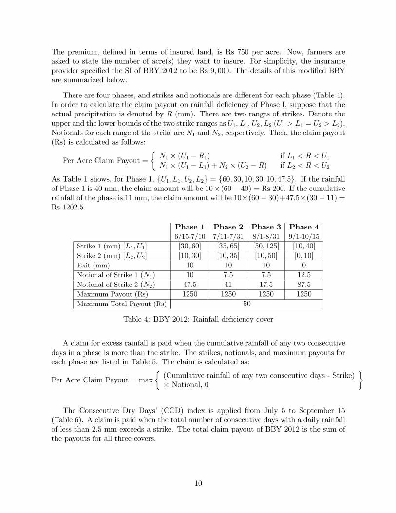
The premium, de�ned in terms of insured land, is Rs 750 per acre. Now, farmers areasked to state the number of acre(s) they want to insure. For simplicity, the insuranceprovider speci�ed the SI of BBY 2012 to be Rs 9; 000. The details of this modi�ed BBYare summarized below.

There are four phases, and strikes and notionals are di¤erent for each phase (Table 4).In order to calculate the claim payout on rainfall de�ciency of Phase I, suppose that theactual precipitation is denoted by R (mm). There are two ranges of strikes. Denote theupper and the lower bounds of the two strike ranges as U1; L1; U2; L2 (U1 > L1 = U2 > L2).Notionals for each range of the strike are N1 and N2, respectively. Then, the claim payout(Rs) is calculated as follows:

Per Acre Claim Payout =�N1 � (U1 �R1)N1 � (U1 � L1) +N2 � (U2 �R)

if L1 < R < U1if L2 < R < U2

As Table 1 shows, for Phase 1, fU1; L1; U2; L2g = f60; 30; 10; 30; 10; 47:5g. If the rainfallof Phase 1 is 40 mm, the claim amount will be 10� (60� 40) = Rs 200. If the cumulativerainfall of the phase is 11 mm, the claim amount will be 10�(60� 30)+47:5�(30� 11) =Rs 1202:5.

Phase 1 Phase 2 Phase 3 Phase 46/15-7/10 7/11-7/31 8/1-8/31 9/1-10/15

Strike 1 (mm) [L1; U1] [30; 60] [35; 65] [50; 125] [10; 40]Strike 2 (mm) [L2; U2] [10; 30] [10; 35] [10; 50] [0; 10]Exit (mm) 10 10 10 0Notional of Strike 1 (N1) 10 7:5 7:5 12:5Notional of Strike 2 (N2) 47:5 41 17:5 87:5Maximum Payout (Rs) 1250 1250 1250 1250Maximum Total Payout (Rs) 50

Table 4: BBY 2012: Rainfall de�ciency cover

A claim for excess rainfall is paid when the cumulative rainfall of any two consecutivedays in a phase is more than the strike. The strikes, notionals, and maximum payouts foreach phase are listed in Table 5. The claim is calculated as:

Per Acre Claim Payout = max�(Cumulative rainfall of any two consecutive days - Strike)� Notional, 0

�

The Consecutive Dry Days� (CCD) index is applied from July 5 to September 15(Table 6). A claim is paid when the total number of consecutive days with a daily rainfallof less than 2.5 mm exceeds a strike. The total claim payout of BBY 2012 is the sum ofthe payouts for all three covers.

10

Phase 1 Phase 2 Phase 3 Phase 46/15-7/10 7/11-7/31 8/1-8/31 9/1-10/15

Strike (mm) 47:5 60 60 62:5Notional (Rs) 5 6 5 5Maximum Payout (Rs) 700 600 600 600

Table 5: BBY 2012: Excess rainfall cover

Cover Period 7/5 - 9/15Strikes (No. of CDD) [L3; U3) [17; 22) [22; 28) [28; 35) [35; 50) [50; 60) [60; 72)Claim Payout (Rs) 175 250 375 500 1000 1500Maximum Payout (Rs) 1500

Table 6: BBY 2012: Consecutive dry days cover

4. Study sites and data

4.1. Study sites, sampling strategy, and primary surveys

Madhya Pradesh is a state in central India (Figure 1). This is the second largest stateof the country, with a population of more than 75 million. In this chapter, I focus on theBurhanpur District in the East Nimar region. Burhanpur is located in the southern partof the state, on the border of the state of Maharashtra.

The Burhanpur District is known for its rain-fed agriculture. Tubewells are onlyavailable in a few areas. The major crops of the district are cotton, bananas, soybeans,sugarcane, wheat and vegetables. Table 7 shows the proportions of land in the districtcultivated for these speci�c major crops, in comparison with the total land cultivated inthe state. Cotton is the most important cash crop, occupying the largest share of thegross cultivated area (23.3%). It is a Kharif crop, although its harvest may extend intothe early months of the Rabi season, as it usually takes 6 to 8 months to complete onecrop cycle. The main cereals are jowar (sorghum) in Kharif and wheat in Rabi, both ofwhich are suitable for rain-fed agriculture. These crops are mostly grown for subsistencepurposes. As a whole, cereals account for only 14.8% of the gross cultivated area. Otherimportant cash crops are soybeans and bananas.18 Soybeans are mostly grown as a Kharifcrop, although it is also harvested in Rabi. It is a fairly new crop in Indian agriculture,and its production spread throughout Madhya Pradesh during the 1990s as a cash cropfrom which vegetable oil is extracted. Banana cultivation takes on average two years toharvest. Therefore it is not classi�ed as either a Kharif or Rabi crop.

In the Burhanpur District, formal insurance is not new at all; governmental cropinsurance, motor, property, life, and health insurance have been available for years in someparts of the district. Government crop insurance, introduced in 1985 and originally calledthe Comprehensive Crop Insurance Scheme (CCIS), now called the National AgriculturalInsurance Scheme (NAIS), is provided by the Agriculture Insurance Company of India

18Bananas are classi�ed as �Fruits�in Table 7.

11

Figure 1: Maps of State of Madhya Pradesh and Burhanpur District

Limited (AICI). Under NAIS, insurance for food crops, oilseeds and selected commercialcrops is mandatory for all farmers that borrow from �nancial institutions such as DCCB.19

As BBY is sold through cooperative societies, this is the �rst tier from which I drewthe sample. A cooperative society is an agricultural unit in which each farmer holds ashare. Farmers often visit the cooperative society to purchase inputs such as seeds andfertilizer, and to gather for meetings. Its o¢ ce building is usually located within 5-10minutes from each house on foot or by motorcycle. My strategy was to draw a randomsample of farmers belonging to each cooperative society, with a substantial variation in thegeographical distances between the weather station and the farmers�landholdings. Thisis because the physical distance from the weather station provided me with the proxyfor the basis risk (Section 4.2. discusses this in detail). To obtain precise informationon studied geographical locations and distances, I collected GPS information on all thefarmers�houses, which is discussed in Chapter 2.

Following the above methodology, the sample size of the current study consists of 433farmers. The sampled farmers were active account holders of the DCCB, and were alllandowners.20 As discussed in Section 2, previous literature suggests one reason for lowtake-up of index insurance is a liquidity constraint. However, a unique characteristic of thispaper�s sampling strategy was to target the population that had access to DCCB credit.There were six cooperative societies: Loni, Shahpur, Bambhada, Chapora, Phopnar, andDedtalai (Figure 1). BBY was available in Shahpur, Bambhada, Chapora, and Phopnarsince 2007, but was not available in Loni and Dedtalai because of the insurer�s supply

19In reality, almost no farmer in the current sample is aware of NAIS. No farmer actually has receivedany claim. Clarke et al. (2011) point out that delays in claim settlement of NAIS has been a seriousconcern.20ITGI�s potential clients are farmers who owe the DCCB for seasonal loans or have a positive balance

in their saving accounts. Landless farmers are not eligible to borrow agricultural loans from the DCCB.

12

Burhanpur Madhya Pradesh1000 ha (%) 1000ha (%)

CerealsRice 2.3 (1.17) 1634.9 (4.18)Wheat 10.4 (5.27) 4089.3 (10.45)Maize 3.5 (1.77) 841.8 (2.15)Sorghum (Jowar) 12.8 (6.49) 534.9 (1.37)Total cereals 29.2 (14.79) 7671.6 (19.60)

PulsesChickpea (Gram) 2.5 (1.27) 2655.7 (6.79)Pigeonpea (Arhar, Tur) 3.7 (1.87) 300.5 (0.77)Total pulses 8.5 (4.31) 4383.7 (11.20)

OilseedsSoybeans 14.3 (7.25) 5187.9 (13.25)Total oilseeds 15.0 (7.60) 6544.7 (16.72)

Sugarcane 2.6 (1.32) 77.2 (0.20)Cotton 45.9 (23.26) 618.0 (1.58)Fruits 14.4 (7.31) 48.9 (0.12)Vegetables 0.7 (0.36) 204.2 (0.52)Others 81.0 (41.06) 19592.5 (50.06)Grand total 197.4 (100.00) 39140.7 (100.00)Source: Compiled by the authors using the district-level databasefor Area and Production of Principal Crops in India, Ministry ofAgriculture, Government of India.

Table 7: Area under major crops in Agricultural Year 2006/07

constraints.21 MBY was introduced to all six societies for the �rst time in Rabi 2011/12.As summarized in Table 8, claims were paid in 2007, 2008, and 2012.

Kharif 2007 Kharif 2008 Kharif 2010 Kharif 2011 Rabi 2011/12 Kharif 2012BBY 2007 BBY 2008 BBY 2010 BBY 2011 MBY 2012 BBY 2012

Claim Paid? Y Y N N Y Y

Table 8: History of the index insurance

There are two main crop seasons in India, Kharif and Rabi: a Kharif crop is a mon-soon or autumn crop, with sowing usually occurring in June/July and harvests in Septem-ber/November. A Rabi crop is a dry season or spring crop, dependent on the moisturein the soil from the latest monsoon. In this case, sowing is usually done in Novem-ber/December and harvests in March/April. For this reason, an agricultural year in Indiais de�ned by combining the Kharif and Rabi crops in this order, and I denote it as, forexample, 2011/12 (that is, Kharif 2011 plus Rabi 2011/12). Crop harvesting may extend

21MBY was introduced to all six societies for the �rst time in Rabi 2011/12.

13

into months of the Rabi season, as it would usually take six to eight months to completeone crop cycle. Banana cultivation takes, on average, two years to harvest. A timelineshowing key events covered in the study is presented in Table 9.

The current dataset consists of the information collected in two rounds of surveys.The �rst survey (denoted as �Survey 2011�) was conducted in October-November 2011,when MBY was being sold. The actual claim payout was Rs 157. This was paid to clientsin May-June 2012. The second survey (denoted as �Survey 2012�) was conducted in May-June 2012, when BBY 2012 was being sold. For both surveys, sample farmers were invitedto the buildings of their cooperative societies to be interviewed on the basis of a structuredquestionnaire. Information on past take-up of BBYs was collected in a retrospectiveway from each farmer, and validated by crosschecking it with the administrative datamaintained by the insurance company. Questionnaires used in Surveys 2011 and 2012 areincluded in the Appendix.

October November December January February March AprilMBY Sales Temperature measurement Claim payoutSurvey Survey 2011Rabi Crops Planting Mid-season and harvest

May June July August September October NovemberBBY Sales Rainfall measurementSurvey Survey 2012Kharif Crops Planting Mid-season and harvest

Table 9: Timeline

Table 10 shows the geographical attributes of the sample households across societies.The number of samples collected at each society is proportionate to the size of the society.The mean distance to the weather station is 11:6 km, and the mean altitude (above sealevel) is 267:6 m. The variance in altitude is very small, which implies that the area is�at.

4.2. Measurement of the basis risk

Ideally, to estimate the basis risk, I need detailed precipitation data measured on bothindividual plots and weather stations. However, for this study, installing rain gauges onthe plots of 433 farmers (who often also have multiple plots) was not practically possible,due to �nancial and logistical constraints.22 Giné et al. (2008) used: i) a dummy variable,which takes the value one if a farmer uses accumulated rainfall to decide when to sow andii) the percentage of land used for Kharif crops. These variables are indirect measures of

22Miura and Sakurai (2012) collected rainfall data on individual plots for 48 households in Zambia.

14

Society Obs Mean S.D. Min MaxLoni 54 Altitude (m) 245.18 10.61 211.23 276.45

Distance (km) 1.99 0.29 1.20 3.58Shahpur 82 Altitude (m) 242.08 14.02 188.67 273.71

Distance (km) 4.74 0.12 4.42 5.00Chapora 118 Altitude (m) 256.52 17.43 219.46 298.70

Distance (km) 7.59 1.11 6.21 9.47Bambhada 126 Altitude (m) 262.89 10.49 226.16 294.13

Distance (km) 7.85 1.12 7.71 8.14Phopnar 17 Altitude (m) 286.42 14.48 261.21 306.63

Distance (km) 10.17 0.84 9.14 11.04Dedtalai 36 Altitude (m) 311.66 4.79 299.92 323.09

Distance (km) 37.42 0.74 36.01 38.68Total 433 Altitude (m) 267.58 26.67 188.67 323.09

Distance (km) 11.60 12.87 1.20 38.68Note: Altitude (m) is a vertical distance from the sea level. Distance(km) is the physical length from to the reference station. Summarystatistics under "Total" are for the pooled sample. They thereforedenote the sum of within�and between-society variations.

Table 10: Geographical attributes of the sample by society

basis risk, as Giné et al. (2008) state that an �alternative variable for measuring basisrisk would be the distance to the rain gauge or some other direct measure of the di¤erencein weather between the farm and the weather station.�Mobarak and Rosenzweig (2012a,2012b) used a perceived distance which was reported by the study participants. Thisdistance was converted to zero if the weather stations were situated in the village.23

Instead, I used the physical distance between farmers�houses and the weather sta-tion as a proxy variable for the basis risk. While the physical distance is not a perfectproxy, meteorologists and agronomists claim that the greater the distance the insured�splot is from the meteorological station, the greater the basis risk will be (Fisher et al.2013). This measure is also intuitive in that farmers are likely to estimate their basis risksubjectively on the basis of the di¤erence between the weather near their house and thatat the nearest weather station during the insurance marketing meeting.24 Therefore, Icollected geocodes (latitude, longitude, and altitude) for the weather station and for eachrespondent�s house. In reality farmers may not subjectively calculate the amount of thebasis risk for each plot.25 Therefore having the distance from their houses to the weatherstation is a reasonable proxy.

23The mean of the reported distance was 4 kilometers, with a standard deviation of 5.9 kilometers.24Basis risk can also be caused by other topographical di¤erences in ground contours, slope, etc. These

factors are important, but beyond the scope of this paper.25This was con�rmed from casual conversation with respondents in the �eld.

15

5. Characteristics of sample farmers

Both Surveys 2011 and 2012 collected detailed information on the sample farmers�socio-economic characteristics, such as family roster, assets, income, agricultural activities,insurance take-up, claim receipts, and consumption. The following tables present thesummary statistics.

5.1. Basic characteristics

Table 11 summarizes the sample�s socio-economic characteristics. The average age ofthe farmers is 51:4 years old, and the average household size is 5:48: The farmers havereceived an average of 6:42 years of education, and have a literacy rate of 52:9%. This levelof literacy is comparable to the state-wide level of 57:8% (rural areas only):26 12:6% of thesample belong to the Scheduled Caste (SC) or Scheduled Tribe (ST),27 and the majorityof the sample (81:6%) belongs to the Other Backward Caste (OBC). Though 62:8% ofthem have access to wells, they still don�t have enough water supply for agricultural uses:they pay an average of Rs 15; 069 (USD 244:8) to rent motor pumps from their neighborsduring Kharif. Indeed, 88:4% of them answered that weather risk is the biggest risk thatthey face.28

Table 11 also lists summary statistics on assets and farming activities. As alreadydescribed, all sample farmers own land. The average landholding size of the sample farm-ers is 4:7 acres. This is slightly larger than the average landholding size of all farmers inMadhya Pradesh (3:68 acres in 2003),29 indicating that my sample does not dispropor-tionately represent wealthy farmers, but contains a number of small and medium farmers.Of the 4:7 acres of average landholdings, 4:03 acres are irrigated.30 The average value ofa house is Rs 334; 728:3 (that is, USD 5437:4).

Table 11 also reports the total agricultural income for each season. The total agricul-tural income during Kharif 2011 is Rs 135; 687:9 (= USD 2218:7).31 The average valueof the loans the sample farmers received just prior to the Kharif growing season was Rs85; 584:0 (= USD 1399:41). The total agricultural income during Rabi 2011/12 was Rs111; 217:5 (= USD 1818:6), while the average loan provided at the beginning of this periodwas Rs 63; 787:0 (= USD 1036:2).

In the sample, 97% of the farmers were clients of IFFCO, the fertilizer company. Thisfamiliarity with the parent fertilizer company played an important role in enabling the26Census 2011.2729:4% of the entire population of the state belong to the SC/ST (Census 2011).28Farmers were asked to rank di¤erent kinds of risks (weather risk, price risk, lack of money, lack of

family labor, lack of land, and lack of infrastructure) from the most to least serious. This question istaken from Cole et al. (2013) where 89% of the sampled households cite the weather risk as the biggestrisk.29This �gure excludes data on landless households and is taken from Statement 4 (state-wise average

size of household ownership holdings), NSSO (2006), p.15.30The change in landholding between the two surveys was very small.31As of October 11, 2013, the exchange rate is Rs 100 = 1:64 USD.

16

insurance provider to sell its insurance products, by reducing potential farmer mistrust ofthe product and/or provider. The questionnaire also included eight arithmetic questionsto determine the farmers�numeracy. The average number of correct answers was 3:1 (S.D.3:4).

Areas under each crop as owned by the sample farmers are also listed in Table 11.32

Consistent with state-wide statistics, area under cotton is the largest throughout theagricultural year. The area under bananas is much higher than the district average (Table7), suggesting that my sample comprises farmers with a stronger commercial orientationthan the district average. After cotton and banana, jowar accounts for about 3:6% inKharif, and wheat for 10:5%. These crops are highly susceptible to extreme weather.

5.2. The take-up of weather insurance

The incidence and depth with respect to the take-up of MBY and BBY are summarizedin Table 12. 24% of the farmers had purchased BBY prior to the current project. Thislow level of penetration is consistent with existing studies.33

In late 2011, 72% of the respondents purchased MBY 2012. This take-up rate isextremely high when compared to existing studies, however, it might not be surprising:my sample di¤ers substantially from that of the existing studies in that the income levelis higher, credit constraints are less likely to be binding, and index insurance is notat all new. In 2012, BBY was sold prior to the monsoon season and was purchasedby 41% of the respondents. The decrease in the take-up rate of BBY 2012 might bebecause people were disappointed by the small (yet positive) claim amount (Rs 157)from the previous season. Also, there is a substantial heterogeneity in the take-up acrosscooperative societies. Detailed discussion on this is provided in Section 5:3:

The experimental procedure was identical between MBY 2012 (Survey 2011) and BBY2012 (Survey 2012). The ITGI market price of Rs 576 (= USD 9:4) per acre was presentedto elicit the farmers�individual index insurance demand, i.e. the number of acres a farmerwould pay to have covered at that price. Then the interviewers o¤ered four di¤erent levelsof subsidy (0%, 25%, 50%, and 75%) if a farmer chose to participate in the study andbuy insurance. A 0% subsidy is equivalent to o¤ering the product at ITGI�s market price,Rs 576. Next, the subject was asked to specify their demand in terms of acres at eachsubsidized price level (the insurance products were sold in 0:5-acre increments). By usingthis method, I elicited four price-quantity pairs per subject. Then, the subjects rolled aneight-sided dice. Each face value of the dice corresponded to the four options (1 and 2to receive a 0% subsidy, 3 and 4 to receive a 25% subsidy, 5 and 6 for 50%, and 7 and 8for 75%). Suppose a farmer answered 0 acres for 0%, 0:5 acres for 25%, 1 acre for 50%,and 2 acres for 75%. If the number on the dice he rolled was 7, then the actual amount

32The area under cotton in Rabi 2011/12 shows the percentage of land occupied by cotton belongingto the Kharif 2011 crops. The numbers for Kharif 2012 were planned ones because Survey 2012 wasconducted right before Kharif 2012. Disbursement of the Kharif crop loan was also in process.33As mentioned before, the take-up rates of brand-new index insurance products implemented by Gine

et al. (2008), Cai (2012) and Cole et al. (2013) were 4:6%; 20% and 23%; respectively.

17

Mean S.D. Min MaxCharacteristics of Respondent

Age 51.4 12.9 20 88Household Size 5.48 2.26 1 15Education (years) 6.42 5.03 0 18Literacy (%) 52.9Score in arithmetic questions 3.1 3.4 0 8SC/ST(%) 12.6Share of OBC (%) 81.6Access to Well (%) 62.8Payment for irrigation usage (Rs) 15069 22789 0 200000Answered weather risk as the biggest risk (%)� 88.4

Major assets at the time of Survey 2011Landholdings (acre) 4.70 5.05 0.25 60Irrigated land (acre) 4.03 5.02 0 60House value (Rs) 334728 538397 0 7000000

Agricultural production during Kharif 2011Area under cotton (%) 52.1Area under banana (%) 29.3Area under maize (%) 7.9Area under jowar (%) 3.6Area under soybeans (%) 4.4Total income (Rs) 135687 167960 0 1500000Crop loan from DCCB (Rs) 85584 104234 0 1280000

Agricultural production during Rabi 2011/12Area under cotton (%) 22.2Area under banana (%) 45.2Area under wheat (%) 10.5Area under maize (%) 13.9Area under jowar (%) 3.3Client of MBY (%) 0.72 0.45Average insured land under MBY (acre)�� 1.14 0.74 0.5 10Total income (Rs) 111217 125821 0 100000000Crop loan from DCCB (Rs) 63787 64339 0 440000

Agricultural production during Kharif 2012Area under cotton (%) 58.2Area under banana (%) 19.2Area under maize (%) 10.8Area under sorghum (%) 4.7Area under soybean (%) 5.0Client of BBY (%) 0.39 0.48Average insured land under MBY (acre)�� 1.00 0.88 0.5 10Crop loan from DCCB (Rs)��� 43474 63372 0 600000

Note: * This is the number of correctly answered questions out of 8 questions. ** This isthe average among those who purchased the insurance. *** The disbursement of Kharif2012 loan was in process.

Table 11: Characteristics of the sample farmers18

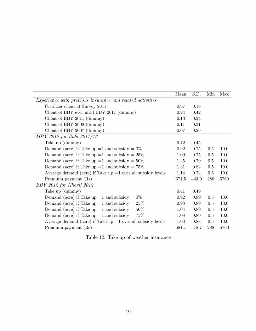
Mean S.D. Min MaxExperience with previous insurance and related activities

Fertilizer client at Survey 2011 0.97 0.16Client of BBY ever until BBY 2011 (dummy) 0.24 0.42Client of BBY 2011 (dummy) 0.13 0.34Client of BBY 2008 (dummy) 0.11 0.31Client of BBY 2007 (dummy) 0.07 0.26

MBY 2012 for Rabi 2011/12Take up (dummy) 0.72 0.45Demand (acre) if Take up =1 and subsidy = 0% 0.92 0.75 0.5 10.0Demand (acre) if Take up =1 and subsidy = 25% 1.09 0.75 0.5 10.0Demand (acre) if Take up =1 and subsidy = 50% 1.25 0.79 0.5 10.0Demand (acre) if Take up =1 and subsidy = 75% 1.31 0.82 0.5 10.0Average demand (acre) if Take up =1 over all subsidy levels 1.14 0.74 0.5 10.0Premium payment (Rs) 671.5 443.0 288 5760

BBY 2012 for Kharif 2012Take up (dummy) 0.41 0.49Demand (acre) if Take up =1 and subsidy = 0% 0.92 0.89 0.5 10.0Demand (acre) if Take up =1 and subsidy = 25% 0.98 0.89 0.5 10.0Demand (acre) if Take up =1 and subsidy = 50% 1.04 0.89 0.5 10.0Demand (acre) if Take up =1 and subsidy = 75% 1.08 0.89 0.5 10.0Average demand (acre) if Take up =1 over all subsidy levels 1.00 0.88 0.5 10.0Premium payment (Rs) 581.1 518.7 288 5760

Table 12: Take-up of weather insurance

19

payable by him would be 576� 2� 75% = Rs 864. The di¤erence between the subsidizedprice and the market price was the amount paid to the subject by the author. The resultsof this subsidy experiment are summarized in Table 12. The table shows that insurancedemand is a decreasing function of insurance price for both MBY and BBY. It is notablethat demand function of MBY is more price-sensitive. This may be because people aremore likely to experiment the brand-new temperature insurance if the premium is low.

As discussed earlier, there were 116 and 255 farmers who didn�t take up MBY or BBY.Among those whose demand for MBY was positive but inelastic, 13 farmers demanded0:5 acres, 123 farmers demanded 1 acre, and 12 farmers demanded 2 acres, regardlessof the price. For BBY, 52 farmers demanded 0:5 acres, 68 farmers demanded 1 acre,and 14 farmers demanded 2 acres, regardless of the price.34 As shown in those �gures,one farmer demanded 10 acres for all the four prices for both products. I treat thisobservation as an outlier in the next chapter.35 Interestingly, 64% and 91% of the 433farmers demanded amounts of acreage coverage which were invariant across the four pricesfor both experiments. Figures 2 and 3 show the distribution of average demand forinelastic and elastic groups, across prices.The insurance demand functions are estimatedand interpreted in further detail in the next chapter.

34This observation is consistent with Cole et al. (2013). In their sample, households almost universallypurchase only one policy unit when they ever do purchase insurance.35The landholding of this farmer was 60 acres. Therefore, the demand in terms of the share of land-

holding is 0:6; which is an average amount in the current sample.

20

050

100

150

0 5 10 0 5 10

inelastic elastic

Freq

uenc

y

Average Demand (acre)Graphs by elastic_mby

Figure 2: Average demand of MBY 2012

010

020

030

0

0 5 10 0 5 10

inelastic elastic

Freq

uenc

y

Average Demand (acre)Graphs by elastic

Figure 3: Average demand of BBY 2012

21

Loni

Shahpur

Chapora

Bambhada

Phopnar

Dedtalai

Survey2011(Baseline)

Landholding(acre)

4.80

3.94

4.93

2.95

11.46

8.44

(2.96)

(3.40)

(4.66)

(2.45)

(13.72)

(6.78)

Irrigatedland(acre)

4.15

3.21

4.39

2.45

11.22

6.68

(2.73)

(3.28)

(4.76)

(2.49)

(13.78)

(6.83)

Literacy�

0.78

0.55

0.63

0.33

0.88

0.31

(0.42)

(0.50)

(0.49)

(0.47)

(0.33)

(0.47)

SC/ST(%)

18.5

9.9

12.8

5.6

5.6

55.6

OBC(%)

88.9

77.8

84.6

92.0

77.8

36.1

Fertilizerclient(%)

0.94

0.96

0.98

0.98

1.0

0.97

Kharif2012

Totalincome(Rs)

159240.7

148993.9

134420.3

93548.8

355352.9

11796.1

(134177.9)

(216155.3)

(138772.1)

(126835.9)

(273099.6)

(159539.4)

Croploanfrom

DCCB(Rs)

127722.2

88634.1

91931.6

55891.3

199529.4

44916.7

(98893.4)(143401.5)

(94262.3)

(51773.7)

(194008.7)

(32948.8)

Areaundercotton(%)

56.3

37.1

46.6

58.1

50.6

68.0

Areaunderbanana(%)

16.4

62.6

30.2

25.4

44.4

0.0

Plannedareaundercotton(%)

55.3

45.3

61.1

67.4

45.2

63.5

Plannedareaunderbanana(%)

16.0

48.6

15.2

11.5

32.3

0.0

BBYTake-up(dummy)

0.15

0.33

0.68

0.30

0.18

0.36

DemandofBBY(acre)��

1.09

1.05

0.90

0.87

1.58

1.71

(0.37)

(0.47)

(0.53)

(0.75)

(0.72)

(2.49)

Table13:Di¤erencesacrosscooperativesocieties

22

Loni

Shahpur

Chapora

Bambhada

Phopnar

Dedtalai

Rabi2011/12

Totalincome(Rs)

146781.6

141720.8

125373.9

48929.73

162271.4

125757.6

(135214.9)

(103845.7)

(138132.7)

(72827.1)

(175838.6)

(159319.8)

Croploanfrom

DCCB(Rs)

87836.7

72402.6

71295.7

38216.2

115928.6

45697.0

(64348.8)

(73207.2)

(66942.8)

(42434.9)

(106423.3)

(27000.6)

Areaundercotton(%)

39.8

30.0

41.5

67.1

41.5

52.1

Areaunderbanana(%)

12.0

56.6

22.2

13.3

25.4

0.0

MBYTake-up(dummy)

0.48

0.73

0.21

0.20

0.47

0.56

DemandofMBY(acre)��

0.94

1.12

1.27

1.06

1.72

1.01

(0.44)

(0.45)

(0.39)

(0.40)

(0.51)

(0.50)

Kharif2012

Croploanfrom

DCCB(Rs)

45426.3

24451.6

62093.5

39269.3

101428.6

20292.9

(Disbursementinprocess)

(57971.3)

(43070.3)

(64626.6)

(68092.7)

(106688.4)

(27410.1)

Plannedareaundercotton(%)

55.3

45.3

61.1

67.4

45.2

63.5

Plannedareaunderbanana(%)

16.0

48.6

15.2

11.5

32.3

0.0

BBYTake-up(dummy)

0.15

0.33

0.68

0.30

0.18

0.36

DemandofBBY(acre)��

1.09

1.05

0.90

0.87

1.58

1.71

(0.37)

(0.47)

(0.53)

(0.75)

(0.72)

(2.49)

Note:Meanisshowninthe�rstrowofeachcategory.S.D.isshowninparenthesis.Correspondingtotalvalues

areintheprevioustables.*literacyoftherespondents.**ifTake-up=1overallsubsidylevels.

Table14:Di¤erencesacrosscooperativesocieties(Continued)

23

020

4060

020

4060

0 5 10 0 5 10 0 5 10

Loni Shahpur Chapora

Bambada Phopnar Dedtalai

Freq

uenc

y

Av erage Demand (acre)Graphs by societycode

Figure 4: Average demand of MBY 2012 by Society

5.3. Di¤erences across cooperative societies

Tables 13 and 14 show that there is a signi�cant amount of heterogeneity in the baselinecharacteristics, farming activities, and insurance-related characteristics across societies.Among the six societies, Phopnar and Loni are the richest societies. Though the averageamount of land owned per household (8:44 ha) is the second largest in Dedtalai, the shareof the irrigated land (79:1%) is the lowest, and this society has the second lowest averageincome. Also the literacy rate of farmers is lowest (31%) in Dedtalai, and the ratio ofSC/ST is also very high (55:56%). Almost all of the farmers in the six societies are clientsof the fertilizer company. Cotton occupies the largest share in the cropping pattern ofall the societies, except Shahpur. Bananas are also very important in all of the societiesexcept Dedtalai, where its cultivation is almost impossible, due to the area�s lack of water.The area of land used for banana cultivation was slightly reduced in Kharif 2012, probablybecause the banana production cycle ended during the previous season. However, giventhat these numbers are only planned �gures, the actual cropping pattern might not bethat di¤erent to that of Kharif 2011.

Demand for BBY 2012 was lower in Loni and Dedtalai than the overall average.This might be attributable to the non-exposure to weather index insurance until Kharif2011;with BBY introduced for the �rst time to those societies in that year. In the caseof Dedtalai, the size of the basis risk may have been responsible, since this society is thefarthest from the weather station (Table 10). Among the four societies with previous

24

020

4060

800

2040

6080

0 5 10 0 5 10 0 5 10

Loni Shahpur Chapora

Bambada Phopnar Dedtalai

Freq

uenc

y

Av erage Demand (acre)Graphs by societycode

Figure 5: Average demand of BBY 2012 by Society

exposure, the demand for BBY 2012 was the highest in Chapora and lowest in Phopnar.It is tempting to deduce that the large basis risk in Phopnar was responsible for thelow demand for insurance (this society is the farthest from the weather station of thefour). However, examining the between-society variation in insurance demand may bemisleading, since it may re�ect other factors such as the di¤erences in income levels,access to irrigation, soil quality, the availability of informal risk-sharing arrangements,and formal risk-coping measures.

6. Conclusion

As an empirical research on weather index insurance in developing countries, I conductedsurveys on rainfall and temperature index insurance products in Madhya Pradesh, India.The rainfall insurance covers drought and excess rain during the monsoon season, whilethe temperature insurance covers against excess heat during the dry season. This chapterdocumented the details of surveys implemented under this project and then described thekey variables collected from them.

Five characteristics of the current study distinguish my dataset from previous studies.First, there exists a wide variation among the sample households with respect to thedistance to the weather station, which gives me the variation in the proxy for basis risk.

25

Second, a quarter of my sample had experience in purchasing the insurance productsprior to my project. This is very di¤erent from previous literature, which focuses on thetake-up behavior of new clients. Third, almost all the households were familiar with thefertilizer company, which is the parent company of the current insurance provider. Thiswould reduce mistrust of the insurer, which previous literature has shown to be one ofthe biggest barriers to insurance take-up. Fourth, I drew my sample from the populationof farmers who had a bank account for crop loans and whose insurance premium wasdeducted from their bank account. This implies that my sample farmers did not faceliquidity constraints. Thanks to the fourth characteristic, by construction, I can excludeliquidity constraints as a reason for the low take-up of weather insurance. It should benoted that my sample covers a wide range of land holding, including small farmers. Fifth,in collaboration with the insurance company, I analyzed the actual insurance productswith real stakes, not hypothetical stakes in a lab, and experimentally changed the pricefor insurance to elicit the individual demand structure. The actual premium amount wasdetermined randomly by rolling a dice.

The descriptive statistics of the data collected in two rounds of surveys in 2011 and2012 show a substantial variation in demand for insurance across households. The take-uprate of the temperature insurance was 72%, which is higher than that described in existingliterature. After six months, the take-up rate of the rainfall insurance declined to 39%, butthe magnitude was still high. We found a wide variation in the demand for insurance acrosscooperative societies through which the insurance product was sold. Some of the variationcould be attributable to the between-society di¤erence in the exposure to insurance saleshistory and the basis risk. However, the results from the descriptive analysis are limitedin their ability to disentangle the various correlated factors.

Distinguishing the impact of each of these factors on insurance demand and quan-tifying the net impact of insurance take-up on household welfare and behavior are leftfor further research. In investigating the determinants of insurance demand, key factorswould be product design, premium rate, basis risk, and trust in the insurer. We collectedinformation on these factors in my two rounds of surveys, and summarized their statis-tics in this chapter. Next chapter will analyze the determinants of insurance take-up,particularly focusing on its relation to the basis risk.

26

Chapter 2Risk Aversion

and Demand for Weather Index Insurance

1. Introduction

As discussed in Chapter 1, the �nancial innovations in index insurance hold signi�cantpromise for rural households (Giné et al. 2008). The take-up rate, while increasing overtime, has been very low. Giné et al. (2008) found the take-up rate to be a mere 4.6%.1 Onlyafter applying intensive marketing interventions, Cai (2012) and Cole et al. (2013) foundsigni�cantly higher take-up rates of 20% and 23%, respectively, which still remain very lowoverall take-up percentages. Existing studies have been trying to identify the barriers thatare discouraging take-up (See Section 2 in Chapter 1). While the results of these studies areplausible, most of them are marginally signi�cant and generally have very small explanatorypower. These results bring a fundamental question: is there any demand for such insurance?

To answer this question, this chapter studies one major disadvantage of index insurance:basis risk. Because there is an imperfect correlation between the weather observed at afarmer�s plot and the weather measured at the reference gauge, there is a discrepancy betweenthe amount of claim payouts from index insurance and the actual production loss of a farmer.This residual risk is called basis risk. In practice, the number of rainfall stations used for theinsurance contract is very limited, and thus claim payouts cannot perfectly cover the exactdamages.

In this chapter, I particularly focus on the relationships among the basis risk, the weatherrisk, and the risk aversion of potential insurance buyers. Standard microeconomic theorypredicts that insurance participation increases with risk aversion, but decreases with basisrisk. There is a trade-o¤ between having extra protection against disaster and bearing thebasis risk. Especially in areas that have many localized climates, the basis risk is high.Existing studies have speculated that basis risk is one of the most important reasons for whyweather index insurance is not attractive to potential clients. Complementing the literature,I investigate a theoretical model of demand for index insurance in consideration of basis risk.With the data described in Chapter 1, I further develop a structural model and estimate therisk aversion parameters.

To the best of my knowledge, this chapter is the �rst study which systematically esti-mates the risk aversion parameters using insurance take-up data. A theoretical study byClarke (2011) is the most closely related to this chapter. He shows that low but inelasticdemand can be explained as an optimal response to the basis risk when the risk aversion ishigh. I estimate the risk aversion parameter and �nd that it is consistent with the observedinelasticity of demand for many farmers. Also, I test whether there is a heterogeneity in therisk aversion with respect to socio-economic characteristics. This is investigated by takingthe estimated risk aversion parameters as a function of various socio-economic characteris-tics. I �nd that age, education, and literacy are negatively correlated with the estimated riskaversion. All the estimated coe¢ cients are statistically signi�cant. Furthermore, I conductover-identi�cation tests and �nd valid models. Finally, I derive an aggregate demand and

1They concluded that, �early in its introduction, the insurance [they] study has not yet succeeded inproportionately reaching the most vulnerable households who presumably would bene�t most from protectionagainst drought.�

28

conduct a counterfactual analysis to quantify the e¤ect of basis risk. I �nd that basis riskis important enough that only farmers within approximately 4km to a weather station canactually reduce the overall risk by purchasing this insurance. These results contribute to thelarge literature studying the role of risk aversion in demand for insurance by being the �rstto explicitly consider basis risk with a rigorous structural model and actual data, and by in-vestigating the relationship between risk aversion and various socio-economic characteristics.I also contribute to research on household �nancial decision-making and risk management.In a broad picture, these results further provide a new insight on technology and productadoption in developing countries.

This chapter is organized as follows. In Section 2, I set up a theoretical model. Section 3explains the method of the structural estimation. Section 4 presents an extension to considerfurther exploration of heterogeneity. Section 5 discusses the link between the model and thedata. Section 6 presents and interprets the estimation results and conducts a counterfactualanalysis. Section 7 presents further discussion, and Section 8 concludes with a summary ofthis paper�s key methods and �ndings.

2. Model

To analyze the demand for insurance, I construct a model of farmers facing weather andbasis risks. Based on Doherty and Shlesinger (1990)�s model, which addresses the e¤ect ofthe risk of non-performance on rational insurance purchases, Clarke (2011) derives a demandfunction under the existence of basis risk, which is a hump shape function as the coe¢ cientof risk aversion increases.2 I adopt Clarke�s (2011) model, but reformulate it by includingcontinuous (and empirical) distributions of production, claim payments, and basis risk.

Consider a (weakly) risk-averse farmer i with an indirect utility function v (�) whichsatis�es the usual properties v0 (�) > 0; v00 (�) � 0.3 He has a non-random endowment wi andhis income Ii depends on wi; agricultural income yi, insurance premium p; and insuranceclaim c. Let y (�) and c (�) be the distributions of agricultural income and claim payments,respectively.4 Both y (�) and c (�) depend on random disturbances (rainfall) denoted by Rwith density g (R) : Let (p; di) be the price (premium) and demand of insurance for i: Thefarmer�s total income is de�ned as Ii = wi + y (R)� dip+ dic (R) :

The farmer decides the amount of demand by solving his expected utility maximizationproblem, given the basis risk. Here, I simply assume that the basis risk is mainly due tothe di¤erence between the weather parameters observed on his plot (R) and on the gauge

2Mahul and Wright (2007) also use Doherty and Shlesinger (1990)�s model and examined demand forinsurance under risk of partial default. They show that optimal actuarially fair coverage of insurance is lessthan full if the recovery rate under default is low.

3The functional form of v (�) is provided in Section 7:1:4Historical production data of the current study site was not available. Therefore, for simplicity, we assume

that the per-acre income distribution y (�) is identical for all farmers. The claim payment distribution c (�)is apparently invariant across farmers as we consider the index insurance. Further details are provided inSection 5.

29

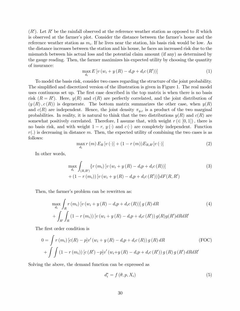
(R0). Let R0 be the rainfall observed at the reference weather station as opposed to R whichis observed at the farmer�s plot. Consider the distance between the farmer�s house and thereference weather station as mi: If he lives near the station, his basis risk would be low. Asthe distance increases between the station and his house, he faces an increased risk due to themismatch between his actual loss and the potential claim amount (if any) as determined bythe gauge reading. Then, the farmer maximizes his expected utility by choosing the quantityof insurance:

maxdiE [v (wi + y (R)� dip+ dic (R0))] (1)

To model the basis risk, consider two cases regarding the structure of the joint probability.The simpli�ed and discretized version of the illustration is given in Figure 1. The real modeluses continuous set up. The �rst case described in the top matrix is when there is no basisrisk (R = R0). Here, y(R) and c(R) are perfectly correlated, and the joint distribution of(y (R) ; c (R)) is degenerate. The bottom matrix summarizes the other case, when y(R)and c(R) are independent. Hence, the joint density �y;c is a product of the two marginalprobabilities. In reality, it is natural to think that the two distributions y(R) and c(R) aresomewhat positively correlated. Therefore, I assume that, with weight r (2 [0; 1]) ; there isno basis risk, and with weight 1 � r; y (�) and c (�) are completely independent. Functionr(:) is decreasing in distance m. Then, the expected utility of combining the two cases is asfollows:

maxdir (m)ER [v (�)] + (1� r (m))ER;R0 [v (�)] (2)

In other words,

maxdi

Z(R;R0)

fr (mi) [v (wi + y (R)� dip+ dic (R))] (3)

+(1� r (mi)) [v (wi + y (R)� dip+ dic (R0))gdF (R;R0)

Then, the farmer�s problem can be rewritten as:

maxdi

ZR

r (mi) [v (wi + y (R)� dip+ dic (R))] g (R) dR (4)

+

ZR0

ZR

(1� r (mi)) [v (wi + y (R)� dip+ dic (R0)) g(R)g(R0)dRdR0

The �rst order condition is

0 =

Zr (mi) [c(R)� p]v0 (wi + y (R)� dip+ dic (R)) g (R) dR (FOC)

+

Z Z(1� r (mi)) [c (R

0)�p]v0 (wi+y (R)� dip+ dic (R0)) g (R) g (R0) dRdR0

Solving the above, the demand function can be expressed as

d�i = f (�; p;Xi) (5)

30

Figure 1: Probability structure. The real model uses continuous set up.

where � is a vector of parameters to be estimated,5 and Xi includes mi; wi; y(R) and c(R):The second order condition is satis�ed. My objective is to estimate the farmers�risk aversionfrom the actual data.

Figure 2 describes comparative statics with respect to the risk aversion parameter (�1)under a Constant Absolute Risk Aversion (CARA) utility function. The average values(across farmers) are used for distance (m) and endowment (w) :6 The three lines representdemand (share) at corresponding price levels. The demand corresponding to the estimated�1 in Section 6 is indicated with markers. When determining their level of demand, farmersface a trade-o¤: while an increase in acre coverage reduces the weather risk, it also increasesthe basis risk. Under the current parameter values, the potential cost of incurring additionalbasis risk outweighs the potential bene�t of having additional insurance; the demand functionis decreasing in risk aversion. Farmers�demand levels with respect to prices are as follows.For all price levels, the demand for farmers with lower risk aversion is price-sensitive. Incontrast, the demand for farmers with higher risk aversion is inelastic to price. The costof incurring additional basis risk is larger for those farmers than for those with lower riskaversion. Thus high risk-averse farmers� demand is small even when the price is belowthe actuarially fair level. Consistent with Clarke (2011), low but inelastic demand can beexplained as an optimal response to the basis risk when the risk aversion is high. Whenthe price is much higher than the actuarially fair level, the demand is zero regardless of thedegree of the risk aversion. Buying insurance at this price decreases the minimum possible

5Functional assumptions are discussed in Sectoin 4.1.6Section 5 presents detailed discussion on data.

31

Figure 2: Comparative statics with respect to �1: CARA utility function and the parameterestimated presented in row (8) of Table 6 are used. The distancem and endowment w are evaluatedat sample means values. The demand corresponding to the estimated �1 in Section 6 is indicatedwith markers.

wealth, and no farmers would optimally purchase the insurance.

Figure 3 illustrates the relationship between demand and ex post risk. The horizontal axisshows the demand (share). The vertical axis represents the risk as de�ned in Ligon (2008),which is the di¤erence in the utility of expected income, U (Ey) and the expected utility ofincome, EU (y), and is normalized to 1 when the demand is zero.7 As in Figure 2, CARAutility function and the parameter estimates presented in row (8) of Table 6 are employed.Again, the average values (across farmers) are used for distance (m) and endowment (w) :Note the graph shows the utilities when a farmer buys the current insurance at the marketprice. For example compared to the case when demand is 0, the risk is 1.002 times largerwhen demand is 0.5. The upward sloping curve of the graph exhibits that insurance coverageactually increases the ex post risk. This corresponds to the case when the cost of incurringadditional basis risk outweighs the bene�t of having additional insurance.

7The risk here is only from variability in income.

32

Figure 3: Demand and risk. As de�ned in Ligon (2008), risk is equal to U(Ey) � EU(y). Thisis normalized to 1 when the demand is zero. CARA utility function and the parameter estimatedpresented in row (8) of Table 6 are used. The distance m and endowment w are evaluated atsample means values.

3. GMM estimation

This section discusses the estimation method employed in the current paper: GeneralizedMethod of Moments.8 For farmer i, the prediction error between i�s actual demand di (p)and predicted demand, " (�; p;Xi), is de�ned as9

" (�; p;Xi) � f (�; p;Xi)� di (p) (6)

Allowing that there is heteroskedasticity in the distribution of error across prices, the momentconditions are

E [" (�; p;Xi)] = 0 (7)

Denote the numbers of moment conditions and parameters by L and K: Because I have fourprice levels, L = 4. I consider orthogonality conditions as additional moment conditions inSection 4.2. The model is over-identi�ed if L > K: If so, I conduct over-identi�cation tests.The GMM estimator is the solution to the following:

b� � argmin�

e (�; p;X)T �Wn � e (�; p;X) (8)

8See, for example, Hayashi (2000).9This is a prediction error to a farmer (not to an econometrician), given the expected utility model in

Section 5 is correct.

33

where e (�; p;X) � 1N

Pi "(�; p;Xi) is (L� 1) vector, and Wn is a (L� L) symmetric and

positive de�nite matrix which converges in probability to some symmetric and positive def-inite matrix W: Provided that regularity conditions hold, b� is consistent. Any positivede�nite matrix W will produce a consistent and asymptotically normal GMM estimator.Hansen (1982) showed that the optimal choice for Wn is

�1 � Eh" (�; p;Xi) � " (�; p;Xi)

Ti�1

(9)

Denote the (K � L) Jacobian as S (�) = @e(�)@�: Because b� is consistent, S(b�) converges in

probability to S (�) : Then the asymptotic distribution of the GMM estimator is

pN�b� � �� � N �0; ST (�) � �1 � S (�)��1 : (10)

3.1. 2-step feasible GMM

The problem with actual implementation of the above method is that I cannot compute�1 because, by de�nition, I need to know the value of � which is exactly what I will estimate.Instead, the actual estimation procedure works in two steps.

1. I generate a consistent 1st-step GMM estimator b�(1): This can be done in several waysas GMM produces consistent estimates with any positive de�nite weighting matrix.Here, I take Wn as identity. Then, 1st-step GMM estimator b�(1) is the solution to

min e (�; p;X)T � e (�; p;X) (11)

This estimator is consistent, but not e¢ cient.

2. With b�(1) in hand; the sample analog of the optimal weight is calculated asWn

�b�(1)� ="1

N

Xi

"�b�(1); p;Xi� � "�b�(1); p;Xi�T

#�1(12)

3. Finally, the GMM estimator b�GMM isb�GMM = argmin�

e (�; p;X)T �Wn � e (�; p;X) (13)

This is asymptotically e¢ cient.

3.2. Over-identi�cation test

If L > K; b�GMM is over-identi�ed. That is, the number of moment restrictions L isgreater than the number of parameters. In this case, the minimand is also a test statistic

34

for the validity of these restrictions. Under the null that these restrictions are valid, the teststatistic (Hansen�s J -statistic) is de�ned as:

J = N �

0@ 1N

Xi

e�b�GMM; p;X�!T �Wn

�b�GMM� � 1N

Xi

e�b�GMM; p;X�!

1A (14)� �2(L�K)

4. Speci�cation and extension

4.1. Speci�cation

This subsection provides functional speci�cations. Assume the farmer�s preference satis�esConstant Absolute Risk Aversion (CARA). In particular, I impose v (x) = 1� e��1x; where�1 is the risk aversion parameter:10 Also, I de�ne a weighting function as the following powerand multiplicative form:

r (mi) =

��3

1 +mi

��2(15)

where �1; �2; and �3 are the parameters to be estimated.11 Then �rst order conditionbecomes

0 =

Zr (mi) [c (R)�p]�1 exp f��1 (wi+y (R)�dip+ dic (R)) gg (R) dR

+

Z Z(1� r (mi)) [c(R

0)� p]�1 expf��1(wi + y(R)� dip+ dic(R0))gg(R)g(R0)dRdR0

I estimate �1; �2; and �3 by feasible 2-step GMM in Section 3.1. Section 6: provides theresults.

4.2. Additional moment conditions

This subsection includes orthogonality conditions as additional moment conditions, whichare

E�XTi " (�; p;Xi)

�= 0 (16)

This means that, conditional on Xi, the error distribution has mean zero. Let M be thenumber of socio-economic variables (such as Age or Education) in Xi. Then the set of newmoment conditions is the (L �M)� 1 vector:

E[� (�; p;Xi)] � E�" (�; p;Xi)XTi " (�; p;Xi)

�= 0 (17)

10The subsequent results are qualitatively the same as long as v0 (x) _ e��1x:11�2 2 (0;mi) :

35

Now the optimal weight is the (L �M)� (L �M) matrix:

Wn

�b�(1)� ="1

N

Xi

��b�(1); p;Xi� � � �b�(1); p;Xi�T

#�1(18)

De�ne h (�; p;X) � 1N

Pi � (�; p;Xi) : Then, GMM is the following:

b�GMM = argmin�

h (�; p;X)T �Wn

�b�(1)� � h (�; p;X) (19)

The detailed derivations of the standard errors are presented in the Appendix. Section 6summarizes the estimation results.

4.3. Linear model

There might be a heterogeneity in risk aversion in terms of socio-economic variables. Inparticular, I consider that risk aversion parameter (�1) is a linear function of �+ �X, where� is an intrinsic risk parameter and � is a coe¢ cient which captures external socio-economicfactors in X.12 Here, the socio-economic variables used are {Education, Age, Age2, Literacy,Math}. For example, I hypothesize that a more educated and/or literate farmer is less riskaverse. The derivation of the standard errors are presented in the Appendix. The de�nitionof those variables are provided in Section 5: Section 6:2: presents the estimation results.

4.4. Selection

As discussed in Chapter 1; only 9% (41 farmers) of the sample are price-responsive.This may indicate a systematic di¤erence in household characteristics between those whohave elastic demand and those who don�t. To consider this, I formulate a selection model asfollows (Vella, 1998):

1(elastic) = X� + u (20)

Residual bu = 1�Xb� (21)

X includes socio-economic variables that do a¤ect demand, but not through the riskaversion parameter. For example, society dummies and crop dummies are candidates ofX: The residuals bu are obtained by subtracting the predicted values from one. Then, theresiduals are added to the demand function to take into account the selection. Now therevised demand function includes a polynomial function of the residuals.

d�i = f1 (�; p;Xi) + f2 (bu; �) (22)

where f2 (bu; �) = �1bu+ �2bu212I assume � = 0 in the previous sections.

36

And the vector (�; �) is estimated below. The derivation of the standard errors are pre-sented in the Appendix. Section 6:3: presents the estimation results.

5. Link between the model and the data

The methodologies described in Sections 3 and 4 were applied to real world data to estimatethe key parameters. As discussed in section 4, I calculated the physical distance betweenthe farmers�houses and the weather station for mi (km) as derived from the GPS data. Thevalue of the house (Rs) is used for wi: Other candidates for wi could be monthly income,monthly expenditure or landholdings. Given that income is very seasonal in the currentcontext, and that the expenditure data is noisy, the single house value was a practical choicefor this variable.13 In addition, because the current utility function takes an exponentialform, the choice of wi should not matter.

As discussed in Chapter 1, four di¤erent levels of subsidies were o¤ered to the farmers.For each subsidy level presented to a farmer, he answered the number of acres he would payto have covered at that level. The price that a farmer actually paid per acre at the o¤eredsubsidy levels (0%; 25%; 50%; 75%) were p1; p2; p3; p4, and the corresponding number ofacres demanded were di1; di2; di3; di4:

A major challenge was getting historical production data for the current study site. In-deed, I have only two rounds of production data from the surveys and have limited knowledgeabout the production history of the farms studied. Instead, y (�) is extrapolated using thedata from the Village Level Study (VLS) conducted by the International Crops ResearchInstitute of the Semi-Arid Tropics (ICRISAT) (Singh et al. 1985).14 ICRISAT-VLS providesdetailed time-series panel data (1975-84) on agricultural and non-agricultural productionand pro�ts, assets, investments and household characteristics in India. Here individual netincome (netinccrop_real) is divided by landholdings (landoperated) to create per-acredistribution. The mean per-acre net crop income found in the VLS survey was Rs 28:75while that of the current study was Rs 10660:21. Then, I multiply the entire productiondistribution of the VLS by the di¤erence in means between the two samples in order toadjust the scale. Similarly, the variance is also multiplied by the square of the di¤erencein means. For simplicity, I assume that the per-acre distribution y (�) is identical for allfarmers. Individual income distribution is derived by multiplying the per-acre distributionby individual landholdings.

The distribution of the claim payment c (�) is calculated using the actual rainfall data andthe BBY 2011 policy. The daily rainfall data was obtained from the Indian MeteorologicalDepartment (IMD) and covered the period between 1951 and 2010.15 The original precipita-tion data is aggregated at the monthly level. The histogram of the time-series precipitation

1398% of the sampled farmers own their houses.14The details of VLS data is summarized in Walker and Ryan (1990).15Unfortunately, the IMD data doesn�t cover the current study site, the Burhanpur District, but it covers

the adjacent one, the Khandwa District.

37

data of the Kharif season (June to September) is presented in Figure 4. The vertical lines onthe histogram show the trigger, the de�ciency levels of 30%, 40% and 50%. Using the actualcontract for rainfall index insurance of 2011, I calculate the probabilities corresponding toeach claim rate. As presented in Table 1; the calculated probabilities for 30% and 40% claimrates are 0:1102 and 0:0544, respectively. The standard deviations are computed by thebootstrapping method. In particular, I resample the IMD data 10; 000 times with replace-ment. The estimated standard deviations are small enough (0:004 and 0:003) to justify thecurrent method. There were no observations in the IMD data set which fell below the 50%de�ciency rate. Thus, in lieu of actual observations from the data set, I employ positive butvery small numbers to generate probabilities.16

02

46

Freq

uenc

y

746.7mm30%40%50%

400 600 800 1000 1200 1400Kharif Rainf all (mm)

Source: Indian Meterological Department (Khandwa District 1915-2010)

Figure 4: Rainfall distribution

The linear model discussed in Section 4:3. uses the socio-economic data obtained throughthe 2011 and 2012 surveys. Age is the age of the sampled farmers (mean 51:31; StandardDeviation 13:11). While the BBY policy in the current study is simpler than the indexinsurance products studied in existing papers, it may still be complicated to those who arenot highly educated. Education measures years of schooling,17 and Literacy is equal to one

16Alternatively, to extrapolate the probabilities for the left tail of Figure 4, I �t the Pareto distributionusing the two data points for the 30 and 40% de�ciency rates as indicated in Table 1. The estimatedprobabilities for 50, 60, 70, 80 90 and 100% de�ciency rates are 0.031, 0.019, 0.013, 0.009, 0.007 and 0.005,respectively.17In the questionnaire, farmers were asked to report their educational completion level according to these

categories: 1: Child, 2: Illiterate, 3: Literate but no formal school education, 4: Pre-primary, 5: Class I-IV,

38

Rainfall (mm) De�ciency Rate (%) Claim Rate (%) Probability S.D.538.16 30 10 0.110 0.004461.28 40 15 0.054 0.003384.40 50 25 0.0001 NA307.52 60 35 0.0001 NA230.64 70 45 0.0001 NA153.76 80 75 0.0001 NA76.88 90 90 0.0001 NA0.00 100 100 0.0001 NA

Table 1: De�ciency rate, Claim rates and corresponding probabilities. The standard devia-tions are computed by the bootstrapping method.

when a farmer reported that he is literate. As listed in Table 7; 53% of them are literate(Standard Deviation 0:50). Math is the number of arithmetic questions that the farmeranswered correctly, out of a total of 8 questions. The mean is 3:1 and Standard Deviations3:4 (See Chapter 1).

6. Results

6.1. Full sample

Using the method and functions described earlier, this subsection presents the results of theGMM estimation. Table 2 summarizes the results of the model described in Sections 3 and 4:Rows (1) ; (6) and (7) include the full sample, (2) excludes an outlier,18 and rows (3)�(5) arethe results on the subsamples of either elastic farmers or inelastic farmers.19 The third andfourth columns list corresponding J -statistics and critical values for the over-identi�cationtests (at 99% con�dence level). Rows (1) � (5) estimate �1 by imposing restrictions �2 = 1and �3 = 1: The estimated risk aversion parameter �1 is 6:05 (0:23) and 6:33 (0:21)in rows(1) and (2) ; respectively (standard errors in parentheses).20 Back-of-envelope calculationestimates that the average relative risk aversion (RRA) is around 4.3. This level of RRA isconsistent with Kurosaki and Fafchamps (2002) and Chuang and Schechter (2013).

The estimated �1 is consistent with the observed low demand for insurance discussed inClarke (2011) in the sense that people would need some protection against drought but don�twant to bear excessive basis risk. For subsample estimations, the estimated �1 of the elastic

6: Class V-IX, 7: Passed Class X, 8: Passed Class XII, 9: Graduate, 10: Post graduate, 11: Professional,12: Diploma/Degree. Then each category was converted to numerical years of schooling. While there weresome cases where farmers dropped out and the corresponding conversion is too noisy, this categorization wascon�rmed to be easier for farmers to answer during the pilot survey.18Here I drop one farmer who demands 10 acres regardless of the price.19As mentioned in Section 4.3.2, 392 out of the 433 farmers demanded amounts of acreage coverage which

were invariant across the four prices.20The following results are qualitatively the same when I use the probabilities extrapolated from the �tted

Pareto distribution.

39

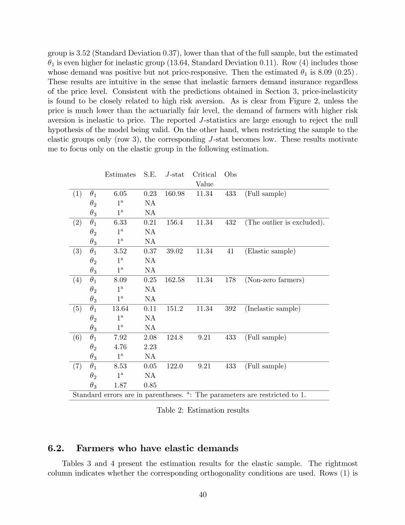
group is 3:52 (Standard Deviation 0:37), lower than that of the full sample, but the estimated�1 is even higher for inelastic group (13:64; Standard Deviation 0:11). Row (4) includes thosewhose demand was positive but not price-responsive. Then the estimated �1 is 8:09 (0:25) :These results are intuitive in the sense that inelastic farmers demand insurance regardlessof the price level. Consistent with the predictions obtained in Section 3, price-inelasticityis found to be closely related to high risk aversion. As is clear from Figure 2, unless theprice is much lower than the actuarially fair level, the demand of farmers with higher riskaversion is inelastic to price. The reported J -statistics are large enough to reject the nullhypothesis of the model being valid. On the other hand, when restricting the sample to theelastic groups only (row 3), the corresponding J -stat becomes low. These results motivateme to focus only on the elastic group in the following estimation.

Estimates S.E. J -stat Critical ObsValue

(1) �1 6.05 0.23 160.98 11.34 433 (Full sample)�2 1a NA�3 1a NA

(2) �1 6.33 0.21 156.4 11.34 432 (The outlier is excluded).�2 1a NA�3 1a NA

(3) �1 3.52 0.37 39.02 11.34 41 (Elastic sample)�2 1a NA�3 1a NA

(4) �1 8.09 0.25 162.58 11.34 178 (Non-zero farmers)�2 1a NA�3 1a NA

(5) �1 13.64 0.11 151.2 11.34 392 (Inelastic sample)�2 1a NA�3 1a NA

(6) �1 7.92 2.08 124.8 9.21 433 (Full sample)�2 4.76 2.23�3 1a NA

(7) �1 8.53 0.05 122.0 9.21 433 (Full sample)�2 1a NA�3 1.87 0.85

Standard errors are in parentheses. a: The parameters are restricted to 1.

Table 2: Estimation results

6.2. Farmers who have elastic demands

Tables 3 and 4 present the estimation results for the elastic sample. The rightmostcolumn indicates whether the corresponding orthogonality conditions are used. Rows (1) is

40

a duplication of (3) in Table 2. Rows (2) and (3) estimate �2 and �3; which found to be4:72 (0:15) and 1:16 (0:07) respectively. Results in row (4) show that �1 is 3:606 (0:001) ; �2is 2:022 (0:066), and �3 is 0:026 (0:046) : As these coe¢ cients are found to be statisticallysigni�cant, basis risk seems to be an important factor. The corresponding J -statistics arestill high enough to reject the over-identi�cation test in these speci�cations.

Then I consider the risk aversion parameter (�1) as a linear function of � + �X: Asexplained in Section 4:3, estimates are generated using the linear model for the di¤erent socio-economic variables, with the results displayed in rows (5)�(20).21 In these speci�cations, theestimated values of the constant are similar to row (1) and signi�cant in all speci�cations.For rows (5) ; (9) ; and (11) ; the coe¢ cients for Education, Math, and Age are �0:169(0:003) ; �0:155 (0:003) ; and �0:004 (0:002) ; respectively (standard errors in parentheses).These speci�cations �t well in the sense that over-identi�cation tests fail to reject the nullhypotheses. The negative and signi�cant coe¢ cients of these variables imply that as yearsof education, and/or number of correct arithmetic answers increase, the level of risk aversiondecreases. As these variables are positively correlated with income, this result is consistentwith the implication of Decreasing Absolute (or Relative) Risk Aversion preferences, in whichone�s level of risk aversion decreases as one�s income increases. For Literacy, the estimatedcoe¢ cients are �0:065 (0:014) and �0:075 (0:007) as shown in rows (7) and (8). This meansthat literate farmers are less risk averse.

Other estimations in the tables use the orthogonality conditions, E[XTi "] = 0 (de�ned

in Section 4.2.), where Xi is either Education, Literacy, Math, Age, or the combination ofthose. Rows (6) ; (10) and (12) show that the estimated coe¢ cients for Education, Math, andAge are �0:106 (0:005) ; �0:109 (0:001) ; and �0:006 (0:002) ; respectively (standard errorsin parentheses). The estimates are signi�cant and similar to those without orthogonalityconditions (rows (5), (9) and (11)), but the reported J -statistics are high. This implies that,while E (") = 0 holds, E

�XTi "�= 0 does not (here X is either Education, Math, or Age).

For rows (15) � (21); the reported J -statistics are also high and the estimates are similarto the cases in which only one of these variables is included. The result of row (22) showsslightly smaller J -statistics, suggesting that �2 and �3 have substantial explanatory powers.

6.3. Selection

Table 5 and Table 6 consider the selection model presented in Section 4:4. First, equation(20) is estimated using a linear probability model (Table 5). The independent variable is abinary variable which takes 1 if one�s demand is elastic. New Society is a binary variablethat takes on the value of one if a farmer belongs either to the Loni or Dedtalai society.Ninety out of the 433 farmers (20:8%) are from those societies. The estimated coe¢ cientfor this variable is negative and generally signi�cant in most of the speci�cations. Possibleinterpretations for why newcomers don�t respond to prices could be because they want to

21As discussed in Section 8, all of the socio-economic variables used in the linear model are converted todeviations from their means.

41

Estimates S.E. J -stat Critical OrthogonalityValue Conditions

(1) �1 3.52 0.37 39.02 11.34 N�2 1a NA�3 1a NA

(2) �1 3.33 0.13 39.27 9.21 N�2 4.72 0.15�3 1a NA

(3) �1 3.87 0.02 38.76 9.21 N�2 1a NA�3 1.16 0.07

(4) �1 3.606 0.001 39.22 6.63 N�2 2.022 0.066�3 0.026 0.046

(5) Const. 4.235 0.008 5.21 9.21 NEducation -0.169 0.003

(6) Const. 3.550 0.004 39.79 16.81 YEducation -0.106 0.005

(7) Const. 3.735 0.004 36.84 9.21 NLiteracy -0.065 0.014

(8) Const. 3.720 0.006 39.58 16.81 YLiteracy -0.075 0.007

(9) Const. 4.110 0.004 5.94 9.21 NMath -0.155 0.003

(10) Const. 3.885 0.003 39.54 16.81 YMath -0.109 0.001

(11) Const. 3.850 0.006 5.68 9.21 NAge -0.004 0.002

(12) Const. 3.651 0.003 39.39 16.81 YAge -0.006 0.002

(13) Const. 3.859 0.026 36.62 6.64 NAge -0.008 0.002Age2 0.003 0.029

(14) Const. 3.233 0.044 39.79 21.66 YAge -0.009 0.001Age2 0.001 0.036

Standard errors are in parentheses. a: The parameters are restricted to 1.

Table 3: Estimation results (Elastic sample)

42

Estimates S.E. J-stat Critical OrthogonalityValue Conditions

(15) Const. 3.619 0.005 39.08 6.64 NAge -0.022 0.002

Education -0.025 0.002(16) Const. 3.856 0.004 39.87 21.66 Y

Age -0.035 0.002Education -0.039 0.001

(17) Const. 3.075 0.147 38.62 6.64 NMath -0.039 0.006

Education -0.001 0.001(18) Const. 3.881 0.003 39.07 6.64 N

Age -0.021 0.001Math -0.086 0.003

(19) Const. 3.881 0.003 39.92 21.66 YAge -0.025 0.002Math -0.105 0.008

(20) Const. 3.026 0.003 39.99 21.66 YMath -0.021 0.001

Education -0.053 0.003(21) Const. 3.642 0.003 39.97 26.21 Y

Age -0.075 0.181Math -0.045 0.087

Education -0.090 0.042(22) Const. 3.143 0.220 37.11 23.21 Y

�2 1.987 0.066�3 0.019 0.005Age -0.081 0.002Math -0.032 0.009

Education -0.046 0.003

Table 4: Estimation Results (Elastic sample, continued)

43

experiment, or they don�t fully understand the products. This result is consistent with thesociety dummies for Loni and Dedtalai having negative estimates. Prior Client is a binaryvariable which takes one if a farmer had experience purchasing an ITGI�s insurance productprior to the project. As summarized in Chapter 1, 24% of the farmers (Standard Deviation0:42) has purchased this product before.

Subjective Purchase BBY/MBY and Subjective Receive Claim are equal to one when afarmer reported that he had purchased ITGI�s insurance prior to the current project, orwhen a farmer answered that he had received claims of any kind of insurance, not just fromITGI. The estimated coe¢ cient for Subjective Purchase BBY/MBY is positive and signi�-cant and that for Subjective Receive Claim is negative and signi�cant, across speci�cations.This indicates that one�s reported experience of having purchased ITGI�s insurance beforeincreases the probability that their demand is price sensitive (this is also consistent with thepositive coe¢ cients estimated for Prior Client), while those who reported previous experi-ence receiving some insurance claims showed less price sensitivity. The absolute (positive)value of the estimated coe¢ cient for the former is higher than the absolute (negative) valueof the estimated coe¢ cient for the latter in all the relevant speci�cations. Thus, the nete¤ect of prior experience with ITGI�s insurance is found to increase the probability of pricesensitivity.

Rain is a binary variable which takes one if a farmer answered that his agricultural workdepends only on rain and/or river. The estimated coe¢ cient for this variable is positivebut not signi�cant. Well is equal to one if a farmer has access to a tubewell or well. Thecoe¢ cient for this variable is negative but not signi�cant. It is notable that (no) access toa well would be highly correlated with income, which is excluded from this regression. Iinterpret these estimated coe¢ cients as indicating that those who have access to wells arerelatively rich and demand insurance regardless of the price. This is consistent with thedummy variable for Phopnar society, which is negative, as this society is the income levelof this society is one of the highest among the six. Each crop that a farmer cultivates isalso assigned a corresponding binary variable, such that if a farmer grows wheat, then thatvariable is 1, if a farmer grows wheat and maize, then each variable takes a value of 1, etc.22

Among the 10 speci�cations, column (9) provides the best �t in terms of the R-squared.

The residuals obtained from estimation (10) of Table 5 are added in the GMM estimationas equations (21) and (22) in Section 4:4. The results are listed in Table 6 (the correspondingorthogonality conditions are included). The estimated coe¢ cients are similar to the onespresented in Table 3, except for the coe¢ cients for the residuals, which are not signi�cantin speci�cations (1) � (7). Adding residuals and their squared terms do not change themagnitude of J -statistics very much. This might be because �2 and �3 are restricted to 1 inthese speci�cations.

22Dummy variables for cotton, bananas, soybeans, sugarcane, wheat, and maize are included.

44

(1) (2) (3) (4) (5) (6) (7) (8) (9)

New Society -0.0775** -0.0769** -0.0662* 0.125 -0.0637(0.0346) (0.0360) (0.0384) (0.291) (0.0410)

Prior Client 0.0227 0.00204 0.0119 0.0139 0.0263 0.0151(0.0337) (0.0349) (0.0365) (0.0353) (0.0368) (0.0359)

Female 0.0394 0.0437 0.0413(0.0422) (0.0430) (0.0428)

HH size -0.00830 -0.00909 -0.00925(0.00625) (0.00621) (0.00633)

Farmer or Ag Labor 0.0317 0.0384 0.0355(0.0306) (0.0306) (0.0303)

Rain 0.0128 0.0248 0.0119(0.0679) (0.0803) (0.0700)

Well -0.0254 -0.0195 -0.0289(0.0304) (0.0312) (0.0314)

SubjectivePurchaseBBYMBY 0.152*** 0.161*** 0.156***(0.0321) (0.0324) (0.0329)

SubjectiveReceiveClaim -0.109*** -0.115*** -0.110***(0.0358) (0.0364) (0.0366)

Shahpur 0.0182 0.0421 0.0185 0.0203(0.0427) (0.0460) (0.0427) (0.0425)

Phopnar -0.0497 -0.0300 -0.0547 -0.0768(0.0745) (0.0768) (0.0761) (0.0774)

Bambada 0.0138 0.0230 0.0148 0.0224(0.0380) (0.0406) (0.0381) (0.0380)

Loni -0.0689 -0.0709 -0.0654 -0.0517(0.0482) (0.0514) (0.0495) (0.0497)

Dedtalai -0.0775 -0.0624 -0.0739 -0.0650(0.0561) (0.0619) (0.0572) (0.0692)

Constant 0.111*** 0.0896*** 0.110*** 0.105*** 0.0572 0.102*** 0.123 0.0480 0.0505(0.0158) (0.0160) (0.0187) (0.0275) (0.0495) (0.0296) (0.0787) (0.0574) (0.0582)

Crop dummy N N N N Y N N N YObservations 433 433 433 430 430 430 430 427 430R-squared 0.012 0.001 0.012 0.014 0.028 0.015 0.076 0.081 0.086

Table 5: Estimation Results (Selection)

Standard errors in parentheses. *** p<0.01, ** p<0.05, * p<0.1

Finally, in row (8) ; the �t becomes better and the model is found to be valid in the sensethat the over-identi�cation test fails to reject the null hypothesis. The coe¢ cients for �2and �3 are estimated to be 2.068 and 1.088. The estimated coe¢ cients for Age, Math andEducation are �0:021; �0:103 and �0:062; respectively, and all are signi�cantly di¤erentfrom zero. These results suggest that older, more educated and/or a farmer with highernumeracy has a higher risk aversion. This can be interpreted as meaning that an older ora more educated farmers are more cautious about risk because they can forecast the risksof the forthcoming season more correctly. The estimated �1(Residual) and �2(Residual2)are 0.005 and 0.003 (both are signi�cant). Modeling the basis risk using the r (m) functionwith power and multiplicative parameters, allowing for heterogeneous risk preferences, andselection increase the explanatory power of the model.

6.4. Aggregate demand and counterfactual analysis

In this subsection, I derive aggregate demand from data and conduct counterfactualanalysis. First, the solid line in Figure 5 illustrates the aggregate demand using the para-meters estimated in (8) of Table 6. This speci�cation includes �2; �3 for the r (m) function,the residual, the residual squared from the selection equation (20 in Section 4.4), and thesocio-economic variables (Age, Math, and Education). This model is preferable for counter-factual analysis because the estimated J -statistics is small and thus the model is proved tobe valid. The average price elasticity of this demand function is -3.11. The absolute valueof the current elasticity exceeds the ones reported in Cole et al. (2011), which are -1.16 to-1.04. Yet, the current price elasticity is reasonable because the sample here includes onlythe farmers who have elastic demand.

It is important to consider how demand changes when the basis risk is reduced. Giventhat the cost of automated rain gauges is not high nowadays, increased density of weatherstations raises the accuracy of the index to proxy the actual production loss. The dashedline in Figure 5 simulates the counterfactual case when there is no basis risk for all farmers(m = 0). The parameters used are the same as the original demand function (solid line).For each price level, demand for insurance substantially increases, which implies that basisrisk is an important factor for farmers. On average the demand increases by 25.3%.

Figure 6 plots the aggregate demand for di¤erent levels of basis risk both for the marketprice and actuarially fair price. The parameters used to derive the demand curves arethe same as the ones used in Figure 5, but now distance (m) is varied in terms of thedensity of weather stations. The horizontal axis plots the density of the weather stations,compared to the real level. I set the density equal to 1, where the real data is used form, as the benchmark case. The density of either 2 (0.5) is the case when the m is halved(doubled) for all farmers. The result is intuitive: the demand increases as the densityincreases, and asymptotically approaches the demand when m = 0: The two points markedin the �gure indicate the thresholds where additional insurance reduces the ex post risk (i.e.,U(Ey)� EU(y) as discussed in Figure 3). In the current sample, reducing the distance (orincreasing the density of weather stations) by around 3 times would decrease the ex post risk.

46

Estimates S.E. J -stat CriticalValue

(1) Const. 3.653 0.029 37.56 16.81Residual -0.040 0.034

(2) Const. 3.690 0.071 39.91 21.67Residual 0.006 0.086Residual2 0.002 0.052

(3) Const. 4.405 0.025 39.73 21.67Age -0.022 0.002

Residual -0.043 0.029(4) Const. 3.553 0.024 39.82 21.67

Education -0.020 0.004Residual -0.033 0.027

(5) Const. 3.681 0.028 39.74 21.67Math -0.110 0.001Residual -0.023 0.031

(6) Const. 3.535 0.020 40.76 30.58Math -0.057 0.001

Education -0.055 0.001Age -0.018 0.002

Residual 0.005 0.022(7) Const. 3.604 0.057 40.98 34.18

Age -0.011 0.001Math -0.058 0.001

Education -0.045 0.004Residual 0.003 0.069Residual2 0.005 0.041

(8) Const. 3.143 0.061 31.86 31.99�2 2.068 0.033�3 1.088 0.016Age -0.021 0.002Math -0.103 0.004

Education -0.062 0.005Residual 0.005 0.002Residual2 0.003 0.001

Table 6: Estimation results (Elastic sample, continued)

47

Figure 5: Aggregate demand, using the parameters estimated in (8) of Table 6.

I �nd that basis risk is important enough that only farmers within approximately 4km to aweather station can actually reduce the overall risk by purchasing this insurance. Thereforeincreasing the density of weather station would have an important e¤ect on the demand.

7. Discussion

This section describes the limitations of the current analysis and discusses remaining issues.First, while the parameter estimates provided in the current paper are informative, they don�tdirectly tell us how bene�cial/harmful the current insurance policy was. Future research willattempt to evaluate this insurance and quantify the welfare impact. This would be importantin the sense that farmers would adopt more pro�table, but riskier varieties or technologieswhen the index insurance is provided. Also, the estimation framework presented in thischapter could be useful to assess the potential long-run outcome of any kind of insurance bysimulating farmers�investment and consumption behaviors.

Second, an inherent aspect of a the structural model, the estimation results depend onthe functional form assumptions. The results reported in the current paper are based onthe CARA utility function and a particular form of the r (m) function. Investigating otherfunctional forms such as Constant Relative Risk Aversion or other Decreasing Absolute RiskAversion utility functions, or other types of r (m) function would be important extensions.Analysis which encompasses these speci�cations is left for future research.

48

Figure 6: Aggregate demand and density of weather stations, using the parameters estimatedin (8) of Table 6. The two points marked in the �gure indicate the thresholds where additionalinsurance reduces ex post risk.

Using multiple indices may be better at predicting production loss (Carter, 2012; Elabedet al. 2013). Total rainfall is the major factor in determining yields such as wheat (Patrick1988), however, with multiple measures, the accuracy of the (combined) index would bemore precise. As described in Chapter 1, the BBY 2012 contract sold to the current sampleuses an excess rainfall index and a consecutive dry days index in addition to the rainfallde�ciency index. Other triggers may include temperature (MBY contract sold by ITGI), theonset date of monsoon (Rosenzweig and Binswanger, 1993, Cole et al. 2013) and satellite-based measures of vegetation density.23 A suitable design of the products that includescombinations of multiple indices would be helpful in reducing basis risk.

Another issue is about to whom weather index insurance should be targeted: micro, meso,or macro level users. The policy investigated in this chapter targeted individual farmers,but as Barnett et al. (2007) claim, it can also be sold to meso-level commercial enterprisessuch as agricultural cooperatives, input suppliers, micro�nance institutions, and local moneylenders. These clients can potentially pool the idiosyncratic risks farmers face. On the otherhand, they face covariate risk. For example, micro�nance institutions or local money lenderswill experience losses when their borrowers default by drought or �ood.24 Local or central

23Carter (2012) suggests the usefulness of satellite-based measure of vegetation density, the NormalizedDi¤erence Vegetation Index (NDVI). NDVI covers 35 countries mostly in Africa. It is notable that NDVIis measured for each 8-km pixel every 10 days. The data is freely available on the Famine Early WarningSystem Network (FEWS NET) website. NDVI is available going back to 1981, meaning that the long-termdata needed to accurately price an insurance index are available (Carter, 2012).24Carter et al. (2012) show that individual weather insurance contracts interlinked with credit might be a

49

government, or donor agencies can also purchase the weather index insurance to pre-�nancesafety-net programs.25 Considering that reinsurance markets are highly developed for suchlarge-scale risks, weather index insurance would be an e¤ective risk transfer mechanism.

8. Conclusion

While micro-insurance markets have been developing in low income countries, the take-uplevels have remained low. This chapter investigates the demand for weather index insuranceby focusing particularly on the relationships among the basis risk, the weather risk, and therisk aversion of potential insurance buyers. I develop a structural model and estimate therisk aversion parameters, and �nd that the estimated risk aversion of the farmers is highenough to explain the inelasticity of the observed demand. Also, this chapter shows that aheterogeneity in socio-economic characteristics a¤ects the level of risk aversion. Furthermore,I derive an aggregate demand and conduct a counterfactual analysis to quantify the e¤ectof basis risk. I �nd that increasing the density of weather stations would decrease the basisrisk and increase the demand for insurance.

The existing papers suggests that micro-insurance markets hold promise to become asigni�cant channel for pooling important sources of household income risk. However, thischapter expresses a more cautious optimism about determining when and how the weatherindex insurance should be employed. The low take-up itself may not be bad at all: dependingon the risk aversions of the potential population, non-purchase may also be a result of farmers�optimal decision-making. Therefore we should be careful about providing subsidies to theinsurance price for the purpose of inducing more farmers to buy the insurance.

Development economists have long recognized how intimately related are the persistenceof poverty and the insurance of various kinds are to each other. It may be useful to identifythe overall impact of introducing a new insurance scheme to farmers�well-being.

better product as lenders may limit the amount of loans to minimize the possibility of covariate default riskof the borrower farmers.25For example, since 2002 the National Fund for Natural Disasters (FONDEN) in Mexico, in collaboration

with the government agricultural insurer (Agrosemex), has been purchasing WII to pre-�nance naturaldisaster assistance (Barnett et al. 2007).

50

Appendix

51

A.1. Standard Errors of �1; �2; and �3The standard errors are derived (10) in Section 3. This can be rewritten as

SE

0B@ b�1b�2b�31CA = diag

1pN�rhST�b�� � �1 � S �b��i�1! (23)

= diag

0BBB@ 1pN�

vuuuut0B@0@de

�b�GMM�db�GMM

1AT

�Wn

�b�GMM� �0@de

�b�GMM�db�GMM

1A1CA�11CCCA

de(b�;p;X)db�GMM =

@f(b�;p;Xi)@b�GMM is calculated by applying the Implicit Function Theorem to FOC

discussed in Section 3. For i = 1; 2; 3;

FOC: (d (�) ;�) = 0 (24)@FOC@d�

� @d�

@b�i + @FOC@b�i = 0 (25)

Thus,df�b�; p;Xi

�db�iGMM = �dFOC

db�i =dFOCdd�(26)

Let � and �0 be � = wi+ y (R)� dip+ dic (R) and �0 = wi+ y (R)� dip+ dic (R0) ; FOCis

0 =R �

�31+mi

��2[c (R)�p]�1 exp (���1) dR+

R R �1�

��3

1+mi

��2�[c (R0)�p]�1 exp (��0�1) dRdR0

(27)

For �1, using Envelope Theorem,

dFOCd�1

=R �

�31+mi

��2[c (R)� p] (���1) exp (���1) dR (28)

+R R �

1��

�31+mi

��2�[c (R0)� pl] (��0�1) exp (��0�1) dRdR0

And,

dFOCdd�

= SOC (29)

=R �

�31+mi

��2[c (R)� p]2

���12

�exp (���1) dR

+R R �

1��

�31+mi

��2�[c (R0)� p]2

���12

�exp (��0�1) dRdR0

52

Similarly, for �2; using Envelope Theorem,

dFOCd�2

= ln�

�31+mi

� R ��3

1+mi

��2[c (R)� p]�1 exp (���1) dR (30)

� ln�

�31+mi

� R R ��3

1+mi

��2[c (R0)� p]�1 exp (��0�1) dRdR0

Finally, for �3;

dFOCd�3

=R �

�2�3

���3

1+mi

��2[c (R)� p]�1 exp (���1) dR (31)

�R R �

�2�3

���3

1+mi

��2[c (R0)� p]�1 exp (��0�1) dRdR0

A.2. Standard Errors of � and �

The standard errors in Section 4:3: are derived as

SE� b�b�

�= diag

0BB@ 1pN�

vuuut24ST �b��

2�4

� �14�4

� S�b��4�2

35�11CCA (32)

= diag

0BBB@ 1pN�

vuuuut0B@0@de

�b�GMM�db�GMM

1AT

�Wn

�b�GMM� �0@de

�b�GMM�db�GMM

1A1CA�11CCCA

53

B. Survey 2011

54

  1

 

KHANDWA BHURUNPUR BBY SURVEY

OCTOBER - NOVEMBER 2011

ID

Date

Mobile Number Start Time   End Time  

 

Interviewee Name Father's Name Address Block ___ ____ _

District ___ ______ Village ________ ____

Society Name Weather station GPS N ˚ ' . ''

E ˚ ' . '' Elevation ft

Distance to W.S. kmDistance to Market km

Interviewer Name

Supervisor Name Completed? □

Version 10/18/11

  2

 

R: Household Roster QR1 QR2 QR3 QR4a QR5

Code

Name

Sex: 1. M 2. F

Relationship to head: See the code

Age?

EducationSee the

code

Occupation

See the code

1 Head 2 3 4 5 6 7 8 9 10 11

12

13

OCCUPATION Child………………………….1 Student…………………………2

Own Farm Activities ......3 Agricultural Labourer ..................4 Casual Labourer, Non Agriculture..5

Salaried Employment .....6 Business, Trade, Manufacturing….7 Unemployed………………..8

Household work...…..9 Others (Aged, Sick, Handicapped etc.)..10 Others (Specify)…………888

EDUCATION

Child………1

Illiterate…………2

Literate but not formal sch

Pre-Primary……….4

Class I – IV……….5

Class V – IX…..…..6

Passed Class X…...7

Passed Class XII.....8

Graduate………....9

Post Graduate……10

Professional……...11

Diploma/Degree12

Others (Specify)………

REALTION WITH THE HEAD

Self……………..1

Wife .......2

Son/Daughter……3

Son-in-law/Daughter-in-law…4

Step son/daughter……………5

Grandchild……………………6

Brother/Sister…………………7

Brother-in-law/Sister-in-law…8

Father/Mother…………………9

Father-in-law/Mother-in-law....10

Other family (specify)………11

Other (specify)…………….888

  3

 

  

M: Mathematics

M1 Please solve the following arithmetic problems. Please use margins for handwriting. Do not use mobile or calculator. Interviewers check whether the answer is correct or not. Illiterate? ( Y N )

(1) 12 + 37 = ( ) (2) 28 + 43 + 13 = ( ) (3) 78 - 19 = ( ) (4) 68 + 17 - 46 = ( ) (5) 8 × 24 = ( ) (6) 23 × 7 = ( ) (7) 48 ÷ 3 = ( ) (8) 104 ÷ 8 = ( )

  4

 

Please tell me whether the household has the following items: YES

NO

If Yes, How Many?

A1 1

2 3 4 5 6 7 8 9 10 11 12 13 14 15 16 17 18 19 20 21 22

Telephone (landline)….…………........ Telephone (mobile)………………….. Clock or watch…………………….… Stove – electric, gas or kerosene…..… Stove - coal, wood (primus)……........ Electric fan.......................................... Television set……… VCR/VCP/CD PLAYER.................... Radio, transistor or stereo.................. Sewing machine……………………. Car or jeep……………………….…. Bicycle………………………….…... Motorcycle, Moped or Scooter..……. Bullock cart………………….……… Thresher……………………..……… Tractor………………………....…… Well/Tubewell....................……… Grain storage can…………..……….. Pressure Cooker…………………….. Table…………………..…………….. Jewelry (silver)………............ Jewelry (gold)...........................

1 1 1 1 1 1 1 1 1 1 1 1 1 1 1 1 1 1 1 1 1 1 1

2 2 2 2 2 2 2 2 2 2 2 2 2 2 2 2 2 2 2 2 2 2 2

XX [ ][ ] [ ][ ]

XX XX

[ ][ ] [ ][ ]

XX [ ][ ] [ ][ ] [ ][ ] [ ][ ] [ ][ ]

XX XX XX

[ ][ ] [ ][ ] [ ][ ] [ ][ ] [ ][ ] [ ][ ]

A2 Does your household own any livestock,

cattle, birds, etc? YES.................................. 1NO.................................... 2DO NOT KNOW...........999

→Next Page →Next Page

Number A3 How many birds does your household own? A4 How many sheep does your household own? A5 How many goats does your household own? A6 How many horses, mules and donkeys does

your household own?

A7 How many cows and oxen does your household own?

A8 How many bullocks does your household own?

A9 How many buffaloes does the household own?

  5

L. Income and Loan

L1 Gross Income from agriculture last Kharif Lakhs

L2 Income from other service work last Kharif

(Specify, Retail shop, Salary ) Lakhs

Remittances received? Rs

L3 Total Income last Kharif (transfer income included) Lakhs

L4 Agricultural loan from society last Kharif Lakhs

L5 Agricultural loan from other bank last Kharif Lakhs

L6 Agricultural loan from society this Rabi Lakhs

L7 Agricultural loan from other bank last Rabi Lakhs

L6 Land holdings Acre

L7 If you want to sell your house, what will be the price? Lakhs

  6

W. Weather Risk

W1. Which risk is the most important to you for your agricultural activities? Which is the 2nd most, 3rd most...?

Weather Risk (drought, monsoon, excess rainfall)

Most important

(please check

✔)

2nd most important

(please

check ✔)

3rd most important

(please

check ✔

Price risk (uncertain price at market)

Lack of money

Lack of family labor

Lack of labor to hire in village

Lack of land

Lack of infrastructure (irrigation, tractor)

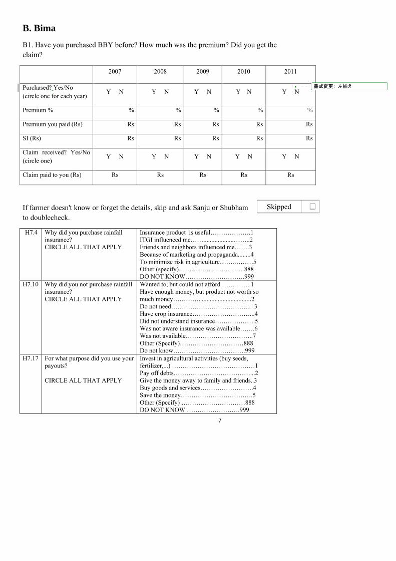
  7

B. Bima

B1. Have you purchased BBY before? How much was the premium? Did you get the claim?

2007 2008 2009 2010 2011

Purchased? Yes/No (circle one for each year)

Y N Y N Y N Y N Y N

Premium % % % % % %

Premium you paid (Rs) Rs Rs Rs Rs Rs

SI (Rs) Rs Rs Rs Rs Rs

Claim received? Yes/No (circle one)

Y N Y N Y N Y N Y N

Claim paid to you (Rs) Rs Rs Rs Rs Rs

If farmer doesn't know or forget the details, skip and ask Sanju or Shubham to doublecheck.

H7.4 Why did you purchase rainfall insurance? CIRCLE ALL THAT APPLY

Insurance product is useful……………….1 ITGI influenced me……...................……..2 Friends and neighbors influenced me…….3 Because of marketing and propaganda........4 To minimize risk in agriculture…….………5 Other (specify)………………………….888 DO NOT KNOW……………………….999

H7.10 Why did you not purchase rainfall insurance? CIRCLE ALL THAT APPLY

Wanted to, but could not afford …………..1 Have enough money, but product not worth so much money………….................................2 Do not need…………………………………3 Have crop insurance………………………...4 Did not understand insurance……………….5 Was not aware insurance was available…….6 Was not available…………………………..7 Other (Specify)…………………………888 Do not know…………………………….999

H7.17 For what purpose did you use your payouts? CIRCLE ALL THAT APPLY

Invest in agricultural activities (buy seeds, fertilizer,...) …………………………………1 Pay off debts………………………………...2 Give the money away to family and friends..3 Buy goods and services…………………….4 Save the money…………………………….5 Other (Specify) …………………………888 DO NOT KNOW …………………….999

Skipped □

書式変更: 左揃え

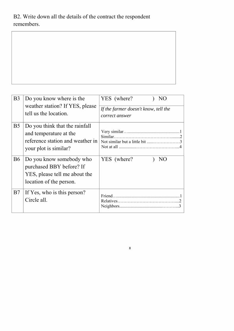
  8

B2. Write down all the details of the contract the respondent remembers.

YES (where? ) NO B3 Do you know where is the weather station? If YES, please tell us the location.

If the farmer doesn't know, tell the correct answer

B5 Do you think that the rainfall and temperature at the reference station and weather in your plot is similar?

Very similar…...............................................1 Similar…………………………………........2 Not similar but a little bit ......………………3 Not at all ................………………………...4

B6 Do you know somebody who purchased BBY before? If YES, please tell me about the location of the person.

YES (where? ) NO

B7 If Yes, who is this person? Circle all.

Friend….........................................................1 Relatives…………………………………....2 Neighbors.......................................………...3

  9

P. Production

P1 How many plots do you have? ( ) plots

P2:

Plot No. 1 2 3 4 5

How far from house?

km km km km km

Total size?

acre acre  acre acre acre 

What Kharif crop?

What Rabi crop?

Irrigation

Tubewell..... 1 Well………...2 Canal.............3 River ............4 Other(Specify) .......................5

Tubewell..... 1 Well………...2 Canal.............3 River ............4 Other(Specify) .......................5

Tubewell..... 1 Well………...2Canal.............3River ............4 Other(Specify).......................5

Tubewell..... 1 Well………...2Canal.............3River ............4 Other(Specify).......................5

Tubewell..... 1 Well………...2 Canal.............3 River ............4 Other(Specify) .......................5

Harvest (kg)

kg kg  kg kg kg 

Revenue (Rs)

Rs Rs  Rs Rs Rs 

Fertilizer (kg)

kg kg  kg kg kg 

  10

 

PLOT INFORMATION B1.7.1 How large is the plot? ACRES……………....................... B1.8.1 In latest Kharif growing season (June-

November 2011), what was the status of this plot? PROMPT FOR THIS QUESTION

Own plot – cultivated by self………………...1 Own plot – cultivated w/ others………….......2 Own plot - rented out…………........................3 Plot rented in.….....…………………………...4 Plot sharecropped………………..…………....5 Own plot – fallow……………..……………...6 Other (specify)……………………...……...888 DO NOT KNOW ….………………………999

B1.13.1

Is the plot cultivated by self? Yes, cultivated by self…………..1 →B1.16 No, cultivated by others…………2 → B1.28

B1.16.1

How much land of the plot did you irrigate?

ACRES…………[ ][ ][ ][ ] DO NOT KNOW…………999

B1.17.1

How much did you spend on irrigation?

Rs:…………………………… Share of output………………. Other (Specify)………………. 888 DO NOT KNOW……………..999

B1.18.1

How much did you spend on other inputs (such as fertilizer, seeds etc). ?

Rs:…………………………… Share of output………………. Other (Specify)………………. 888 DO NOT KNOW……………..999

B1.19.1

Which fertilizer brand and how many fertilizer did you apply hired on this plot?

IFFCO……………………………..................... KHETN...........................................…………. Other (Specify)………………..................... 888

kg kg kg

  11

 

If YES: Cultivated Yes1 No2

for home consumption? Yes 1 No 2

for sale? Yes 1 No 2

Total area planted with the crop

H Y V / G M

U N I T

Qty Price per unit

Total Value of Output

B1.21.1

Did you cultivate any of the following crops on this plot last Kharif? If yes, was it for food, for sale, how much land did you plant with the crop and what is the total value for one year? 1.Rice……………… 2.Bajri…………….. 3.Jowra……………. 4.Wheat…………… 5.Cotton……………. 6.Castor……………. 7.Cumin…………… 8.Groundnut……….. 9.Sesame…………… 10.Tobacco………… 11.Vegetables……… 12.Pulses(Specify) 13.Mustard 14. Soy bean 15. Sugarcane 16. Banana 17. Lily 18. Chili 19.Other (Specify)__

1 2 1 2 1 2 1 2 1 2 1 2 1 2 1 2 1 2 1 2 1 2 1 2 1 2 1 2 1 2 1 2 1 2 1 2 1 2

1 2 1 2 1 2 1 2 1 2 1 2 1 2 1 2 1 2 1 2 1 2 1 2 1 2 1 2 1 2 1 2 1 2 1 2 1 2

1 2 1 2 1 2 1 2 1 2 1 2 1 2 1 2 1 2 1 2 1 2 1 2 1 2 1 2 1 2 1 2 1 2 1 2 1 2

acre ……….. ……….. ……….. ……….. ………. ………. ………. ………. ………. ………. ………. ………. ………. ……….. ……….. ………. ……….. ……….. ………..

1 2 1 2 1 2 1 2 1 2 1 2 1 2 1 2 1 2 1 2 1 2 1 2 1 2 1 2 1 2 1 2 1 2 1 2

B1.22.1 INTERVIEWER CHECKPOINT: Does the household use HYV varieties?

Yes ………………………………..1→B1.24 No…………………………………2→B1.23

B1.23.1 Why do you not use HYV/GM varieties on this plot?

Seeds expensive…………………1 Too risky ……………………….2 Not available for this crop ………3 Not familiar with them ………….4 Other (Specify)………………….888 Do not know ……………………999

B1.24.1 Did you experience any problems on this plot last Kharif (e.g. drought, flood, pests, disease etc.)?

YES………………………….1 →B1.25 NO…………………………...2 → B1.28 DO NOT KNOW………….999→ B1.28

→B1.25

B1.25.1 How much output do you think you lost due to those problems?

Share of potential output……………..% Other (specify)………………………..888 DO NOT KNOW……………………….999

B1.26.1 Why did you keep the land fallow during the last Kharif? RECORD VERBATIM

  12

 

INTERVIEWER READ: Now I’m going to ask you a few questions about use of this plot during the Rabi growing season.

B1.28.1 What is the status during this Rabi ?

Own plot – cultivated by self…………………..…1 Own plot – cultivated w/ other……………………2 Own plot - rented out…………..............................3 Plot rented in.……………………………………..4 Plot sharecropped………………………………....5 Own plot – fallow………………………………....6 Other (specify)……………………………….....888 DO NOT KNOW ….…………………………...999

B1.29.1 How much do you expect to earn from this plot during Rabi 2011-2012?

Much less than usual …………………………1 Less than usual..………………………………2 About the same as usual………………………3 More than usual……………………………….4 Much more than usual…………………………5

B1.30.1 Did inadequate Kharif rains affect your usage of this plot during the current Rabi season?

Yes, was unable to cultivate it as desired……..1 Yes, was forced to take out a loan for inputs….2 Yes, other reason………………………………3 No……………………………………………...4

  13

 

C. Consumption INTERVIEWER CHECKPOINT: Collect data on consumption for each of the following items. Consumption

includes both consumption from own production and expenditures on purchased products. For each item remind respondent to include what they have consumed out of their own production.

C.0 Worksheet for recording household consumer expenditure

Item group value of consumption (Rs) During last 30 days (1) (2)

Unit Qty Price Value 1. cereals & cereal products Rice Wheat Bajiri Other cereals 2. pulses & pulse products 3. milk & milk products 4. edible oil 5. vegetables 6. fruits & nuts 7. egg, fish & meat 8. other food items (sugar, salt, spices, beverages,

processed food, etc.)

9. pan, tobacco & intoxicants 10. fuel & light 12. misc. goods & services (monthly expenditure) 12.1 cinema / theatre / video show 12.2 tuition fees 12.3 newspapers, magazines, fiction 12.4 medical expenses (non-institutional) 12.5 toilet articles including washing soap &

other cleaning agents

12.6 regular (commuting type) and other journeys

12.7 house rent 12.8 other miscellaneous goods & services  

  14

 

C.0 Worksheet for recording household consumer expenditure

Item group value of consumption (Rs) During Last 180 days (1) (2)

13. misc. goods & services (annual expenditure) 13.1 school books & other educational articles 13.2 hospital, nursing home (institutional) 14. clothing 15. footwear 16. durable goods 16.1 furniture 16.2 utensils 16.3 ornaments/jewelry 16.4 kitchen equipment 16.5 vehicles including bicycles 16.6 clocks & watches 16.7 cassettes & records 16.8 TV, radio, etc. 16.9 other household appliances 16.10 repair and maintenance C1 What did you spend in the last 6 months for :

1- weddings 2- funerals 3- festivals ( Govri, Navratri, Holi, Diwali, Rakhi, etc…or other festivals: Eid, Christmas…)

Rs. ……………………….. Rs. ……………………….. Rs………………………….

  15

 

G. SAVINGS G1.1 Does anyone in your household have a savings

account of any kind? YES……………….1 NO…………………2

G1.2 How many savings accounts does the household have?

[ ] accounts

INTERVIEWER CHECKPOINT: ASK QUESTIONS G1.3 TO G1.11 ABOUT EACH SAVINGS ACCOUNT AND RECORD ANSWERS ON GRID ON THE OPPOSITE PAGE.

G1.4 Which type of savings account is this? Bank / Post Office Account …………….1 Other ........................................................2 DON’T KNOW .......................999

G1.5 What is the total balance of this account? If it is a joint account with others not in your household, what is your share of the balance?

Rs. [ ][ ][ ],[ ][ ][ ]

G1.11 What is the interest rate? ……………… % PER MONTH....................1 PER YEAR........................2 DO NOT KNOW............ 999

I: Individual information

QI1 What is your caste? 1. □ General 2. □ SC 3. □ ST (specify: ) 4. □ OBC

QI2 What is the subcaste?

QI3 Religion 1. Hindu 2. Jain 3. Muslim 4. Christian 5. Other (Specify )

  16

H5. RECENT RAINS H5.1 How would you characterize the quality of the

monsoon rains last Kharif? On this ladder, with the top of the ladder being very good and the bottom being extremely poor, where would you place this past monsoon?

1 2 3 4 5 6 7 8 9 10Very Bad……..…………….Excellent DO NOT KNOW………………999

H5.2 Was the rain good for farmers to plant their seeds?

YES…….……………………….1 NO, TOO LITTLE………………2 NO, TOO MUCH……………….3 NO, Other (Specify)…………… 888 DO NOT KNOW………….999

H5.3 Was the rain good for the plants to grow / germinate?

YES…….……………………….1 NO, TOO LITTLE………………2 NO, TOO MUCH……………….3 NO, Other (Specify)…………… 888 DO NOT KNOW………….999

H5.4 Was the rain good during harvest?

YES…….………………………..1 NO, TOO LITTLE………………2 NO, TOO MUCH………………..3 NO, Other (Specify)…………… 888 DO NOT KNOW………….999

H5.5 Did the quality of rain affect the availability of work for people who wanted to work as laborers on farms?

YES………………………………….1 NO……………………………..……2 DO NOT KNOW ………………….999

H5.6 Did the quality of rain affect the availability of food grains?

YES………………………………….1 NO……………………………………2DO NOT KNOW ………………….999

H5.7 Did the quality of the rain affect the price of food grains?

YES, MORE EXPENSIVE …….....1 YES, LESS EXPENSIVE…………2 NO………………….………….......3 OTHER (Specify) …………….......888 DO NOT KNOW …………….…999

H5.8 Do you know what a millimeter is? YES………………………………1 NO………………………………..2

H5.10

H5.9 What is your best estimate of how many millimeters of rain fell from the start of planting until harvest?

……………………………………….

H5.10 Do you think the rains will be good during the upcoming Rabi season?

YES…….……………………….1 NO, TOO LITTLE………………2 NO, TOO MUCH……………….3 NO, Other (Specify)…………… 888 DO NOT KNOW………….999

H5.11 How do you make the prediction of how rains will be this upcoming Rabi?

Last Kharif rainfall…………….1 Last Rabi rainfall……………….2 Based on ‘Normal’ rainfall……..3 Other (Specify)…………………888 DO NOT KNOW………………999

H5.12 What was the value of crop loss due to poor rain fall this past (2011) Kharif season?

RUPEES…[ ][ ][ ][ ][ ] NO LOSS……………………..0

C. Survey 2012

71

  1

BHURHUNPUR BBY SURVEY

MAY 2012

ID

(Old ID) □ Had interview before? (Old ID)

Mobile Number Date Start Time   End Time  

 

Farmer's Name Father's Name Address District .......................

Tehsil ............................. Mandal .......................... Block ............................ Village ...........................

Society Name GPS Completed?

□Yes □No N ˚ ' '' /E ˚ ' '' Elevation feet

Distance to W.S. kmDistance to Market km

Interviewer Name

Supervisor Name Completed? □

Household visit? □

 

 

Version 4/12/12

  2

 

L. Income and Loan

The followings are the income and loan for the whole household

L0 How many people are living together in your house?

L1 Gross Income from agriculture last Rabi Lakhs

L2a Income from other service work last Rabi

(Specify, Retail shop, Salary, other) Which month? ( ) Rs / month

L2b Money received from family or relatives living far? Rs

L2c Gift from family or relatives living far?

If yes, what was that?

What is the estimated value of that?

□Yes □ No

( )

Rs

L3 Total Income last Rabi (transfer income included) Lakhs

L4 Agricultural loan from society last Rabi Lakhs

L5 Agricultural loan from other bank last Rabi Lakhs

L6 Agricultural loan from society this Kharif 2012 Lakhs

L7 Agricultural loan from other bank last Kharif 2012 Lakhs

  3

B. Bima B1 Did you purchase MBY? □Yes □ No B2a. Have you purchased any kind

of insurance before? If so which policy?

AIC (Govt crop insurance)....................1 ICICI Lombard's property insurance....2 ITGI's micro insurance .........................3 Vehicle insurance ..................................4 Other (NAME )............5

B2b.

Did you receive any claims of that ?

B4a Are you aware that insurance for personal accident is provided with IFFCO's fertilizer?

□Yes □ No

B4b If Yes, have you ever received any claims?

□Yes

□ No

C1a Where does the household get most of the drinking water? 1 Piped water at home

2 Public tap

3 Private well

4 Public well

5 River/stream

6 Pond/Lake

C1b

How far is the place where you collect water? 1 At home

2 ( km)

  4

P. Production: How many plots do you have? ( ) plots

Plot No. 1 2 3 4 5

Size acre acre acre acre  acre

Rabi 2012 Crop

Harvest kg kg kg kg kg

Revenue Rs Rs Rs Rs Rs

Seeds (Inputs)

Rs Rs Rs Rs Rs

Manure kg kg kg kg kg

Fertilizer kg kg kg kg kg

Fertilizer Brand

IFFCO ( kg) KHETN( kg) URIA ( kg) POTASH ( kg) PHOSPATE( kg)

IFFCO ( kg) KHETN( kg) URIA ( kg) POTASH ( kg) PHOSPATE( kg)

IFFCO ( kg) KHETN( kg) URIA ( kg) POTASH ( kg) PHOSPATE( kg)

IFFCO ( kg) KHETN( kg) URIA ( kg) POTASH ( kg) PHOSPATE( kg)

IFFCO ( kg) KHETN( kg) URIA ( kg) POTASH ( kg) PHOSPATE( kg)

Kharif 2012 Crop (Planned)

Harvest (Expected)

kg kg kg kg kg

Revenue (Expected)

Rs Rs Rs Rs Rs

Seeds (Expected)

Rs Rs Rs Rs Rs

Manure (Expected)

kg kg kg kg kg

Fertilizer (Expected)

kg kg kg kg kg

Fertilizer

Brand

IFFCO.( kg) KHETN( kg) URIA ( kg) POTASH ( kg) PHOSPATE( kg)

IFFCO.( kg) KHETN( kg) URIA ( kg) POTASH ( kg) PHOSPATE( kg)

IFFCO.( kg) KHETN( kg) URIA ( kg) POTASH ( kg) PHOSPATE( kg)

IFFCO.( kg) KHETN( kg) URIA ( kg) POTASH ( kg) PHOSPATE( kg)

IFFCO.( kg) KHETN( kg) URIA ( kg) POTASH ( kg) PHOSPATE( kg)

Irrigation

Tubewell........... ..1 Well……….........2 Canal....................3 River ...................4 Neighbor's help....5 Motor pump.........6 Rain only ............7 Other(Name )....8

Tubewell........... ..1 Well………..........2 Canal....................3 River ...................4 Neighbor's help....5 Motor pump.........6 Rain only ............7 Other(Name )....8

Tubewell........... ..1 Well………..........2 Canal....................3 River ...................4 Neighbor's help....5 Motor pump.........6 Rain only ............7 Other(Name )....8

Tubewell........... ..1 Well………..........2 Canal....................3 River ...................4 Neighbor's help....5 Motor pump.........6 Rain only ............7 Other(Name )....8

Tubewell........... ..1 Well………..........2 Canal....................3 River ...................4 Neighbor's help....5 Motor pump.........6 Rain only ............7 Other(Name )....8

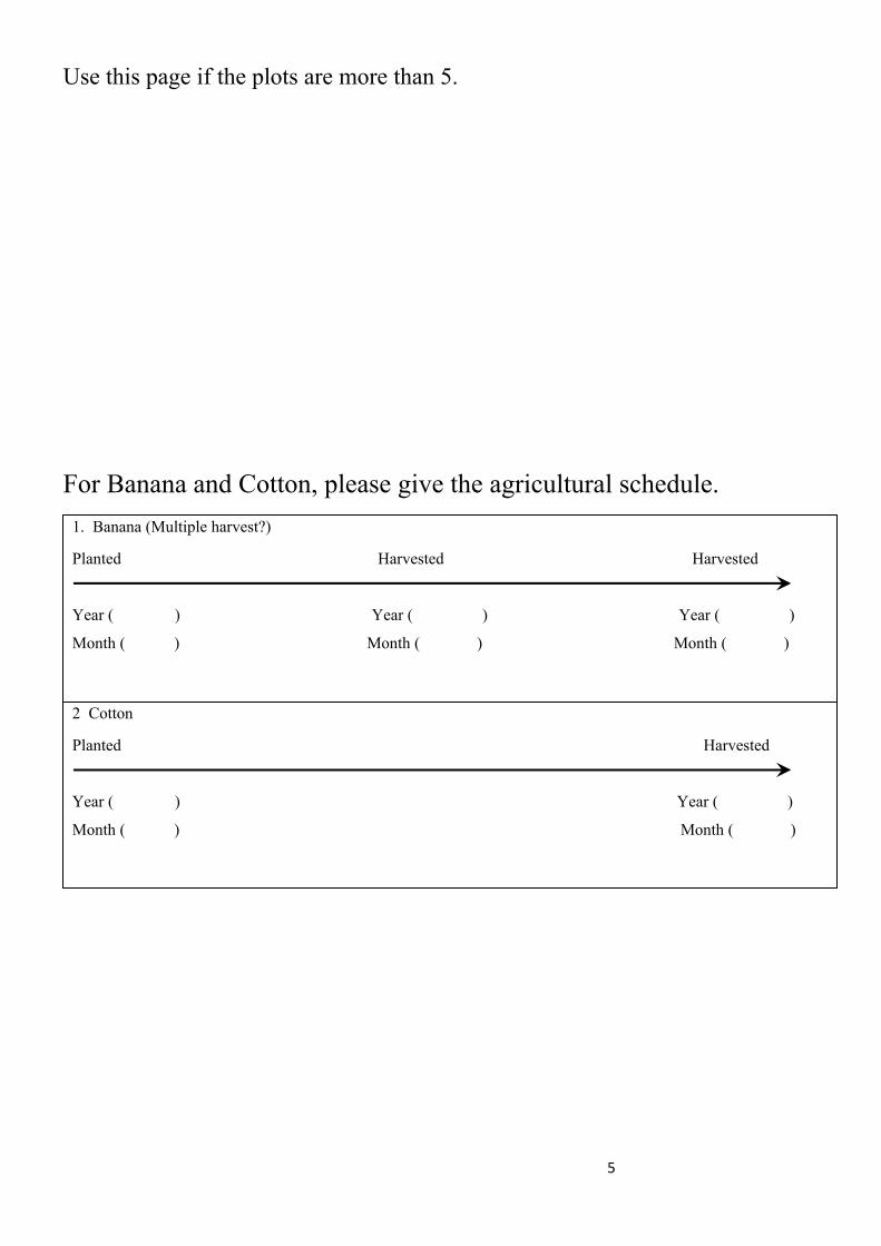
  5

Use this page if the plots are more than 5.

For Banana and Cotton, please give the agricultural schedule.

1. Banana (Multiple harvest?)

Planted Harvested Harvested

Year ( ) Year ( ) Year ( )

Month ( ) Month ( ) Month ( )

 

2 Cotton

Planted Harvested

Year ( ) Year ( )

Month ( ) Month ( )

 

  6

for home consumption? Yes 1 No 2

for sale? Yes 1 No 2

Total area planted with the crop

H Y V / G M

U N I T kg liter

Qty

Price per unit

Total Value of Output

C21.

Did you cultivate any of the following crops on this plot last Kharif? If yes, was it for food, for sale, how much land did you plant with the crop and what is the total value for one year? 1.Rice……………… 2.Bajri…………….. 3.Jowar……………. 4.Wheat…………… 5.Cotton……………. 6.Castor……………. 7.Cumin…………… 8.Groundnut……….. 9.Sesame…………… 10.Tobacco………… 11.Vegetables……… 12.Pulses(Name...........) 13.Mustard 14. Soy bean 15. Sugarcane 16. Banana 17. Lily 18. Chili 19 Maize 20.Other (Specify)__

1 2 1 2 1 2 1 2 1 2 1 2 1 2 1 2 1 2 1 2 1 2 1 2 1 2 1 2 1 2 1 2 1 2 1 2 1 2 1 2

1 2 1 2 1 2 1 2 1 2 1 2 1 2 1 2 1 2 1 2 1 2 1 2 1 2 1 2 1 2 1 2 1 2 1 2 1 2 1 2

acre ……….. ……….. ……….. ……….. ………. ………. ………. ………. ………. ………. ………. ………. ………. ……….. ……….. ………. ……….. ……….. ……….. ………..

1 2 1 2 1 2 1 2 1 2 1 2 1 2 1 2 1 2 1 2 1 2 1 2 1 2 1 2 1 2 1 2 1 2 1 2 1 2

C22 INTERVIEWER CHECKPOINT: Does the household use HYV varieties?

Yes ………………………………..1→B1.24 No…………………………………2→B1.23

C23 Why do you not use HYV/GM varieties on this plot?

Seeds expensive…………………1 Too risky ……………………….2 Not available for this crop ………3 Not familiar with them ………….4 Other (Specify)………………….888 Do not know ……………………999

C24 Did you experience any problems on this plot last Kharif (e.g. drought, flood, pests, disease etc.)?

YES………………………….1 →B1.25 NO…………………………...2 → B1.28 DO NOT KNOW………….999→ B1.28

B1.25

C25 What kind of problem is this? Drought .(water is not enough)...............................1

Pest..........................................................................2 Temperature is too high..........................................3 Crop disease ...........................................................4 Flood (water is too much) .......................................5

C26 How much output do you think you lost due to those problems?

Share of potential output……………..% Other (specify)………………………..888 DO NOT KNOW……………………….999

A × B = C

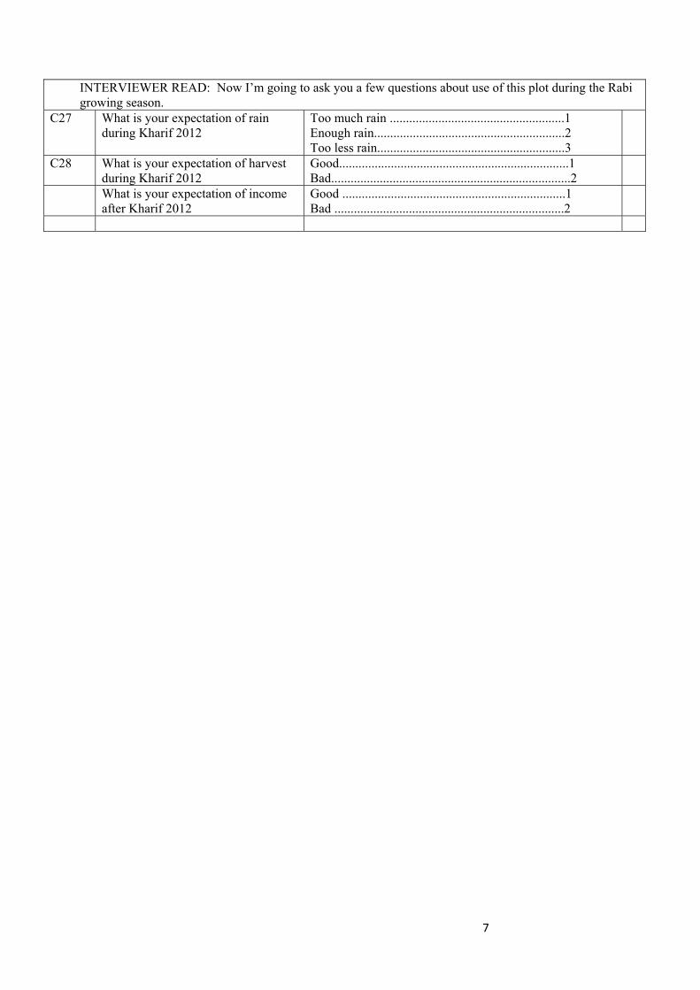
  7

 

INTERVIEWER READ: Now I’m going to ask you a few questions about use of this plot during the Rabi growing season.

C27 What is your expectation of rain during Kharif 2012

Too much rain ......................................................1 Enough rain...........................................................2 Too less rain..........................................................3

C28 What is your expectation of harvest during Kharif 2012

Good.......................................................................1 Bad..........................................................................2

What is your expectation of income after Kharif 2012

Good .....................................................................1 Bad .......................................................................2

 

 

  8

 

C. Consumption INTERVIEWER CHECKPOINT: Collect data on consumption for each of the following items. Consumption

includes both consumption from own production and expenditures on purchased products. For each item remind respondent to include what they have consumed out of their own production.

C.0 Worksheet for recording household consumer expenditure

Item group value of consumption (Rs) During last month April 2012 (1) (2)

Unit Qty Price Value 1. cereals & cereal products Rice Wheat Jowar Bajiri Other cereals 2. pulses & pulse products 3. milk & milk products 4. edible oil 5. vegetables 6. fruits & nuts 7. egg, fish & meat 8. other food items (sugar, salt, spices, beverages,

processed food, etc.)

9. pan, tobacco & intoxicants 10. fuel & light 12. misc. goods & services (monthly expenditure) 12.1 cinema / theatre / video show 12.2 tuition fees 12.3 newspapers, magazines, fiction 12.4 medical expenses (non-institutional) 12.5 toilet articles including washing soap &

other cleaning agents

12.6 regular (commuting type) and other journeys

12.7 house rent 12.8 other miscellaneous goods & services  

  9

 

C.0 Worksheet for recording household consumer expenditure

Item group value of consumption (Rs) During Last 180 days (Nov, Dec, Jan, Feb, Mar, Apr) (1) (2)

13. misc. goods & services (annual expenditure) v vvv 13.1 school books & other educational articles 13.2 hospital, nursing home (institutional) 14. clothing 15. footwear 16. durable goods v vvv 16.1 furniture 16.2 utensils 16.3 ornaments/jewelry 16.4 kitchen equipment 16.5 vehicles including bicycles 16.6 clocks & watches 16.7 cassettes & records 16.8 TV, radio, etc. 16.9 other household appliances 16.10 repair and maintenance C1 What did you spend in the last 6 months for :

1- weddings 2- funerals 3- festivals ( Govri, Navratri, Holi, Diwali, Rakhi, etc…or other festivals: Eid, Christmas…)

Rs. ……………………….. Rs. ……………………….. Rs………………………….

 

 

  10 

Game In this game, we will offer you four BBY products, called B1, B2, B3 and B4. B1 is the original premium without discounts. For each of the four options, please decide whether you want to purchase the BBY at that premium. If you want, you probably have a chance to get a discount. Please state the amount of the Sum Insured (Rs). At the end of the two game sessions, we will let you throw a dice with 8 numbers. The number of the dice corresponds to each option. You will be given a subsidy of the option you draw, or up to the maximum of Rs 576.

Subsidy (%)

Premium (Rs)

Purchase?Y/N

If Y, how much SI do you want?

Dice

B1 0% 576 Rs Y N Rs 1, 2

B2 25% 432 Rs Y N Rs 3, 4

B3 50% 288 Rs Y N Rs 5, 6

B4 75% 144 Rs Y N Rs 7, 8

Your Choice Payment Rs

Dice Number Signature

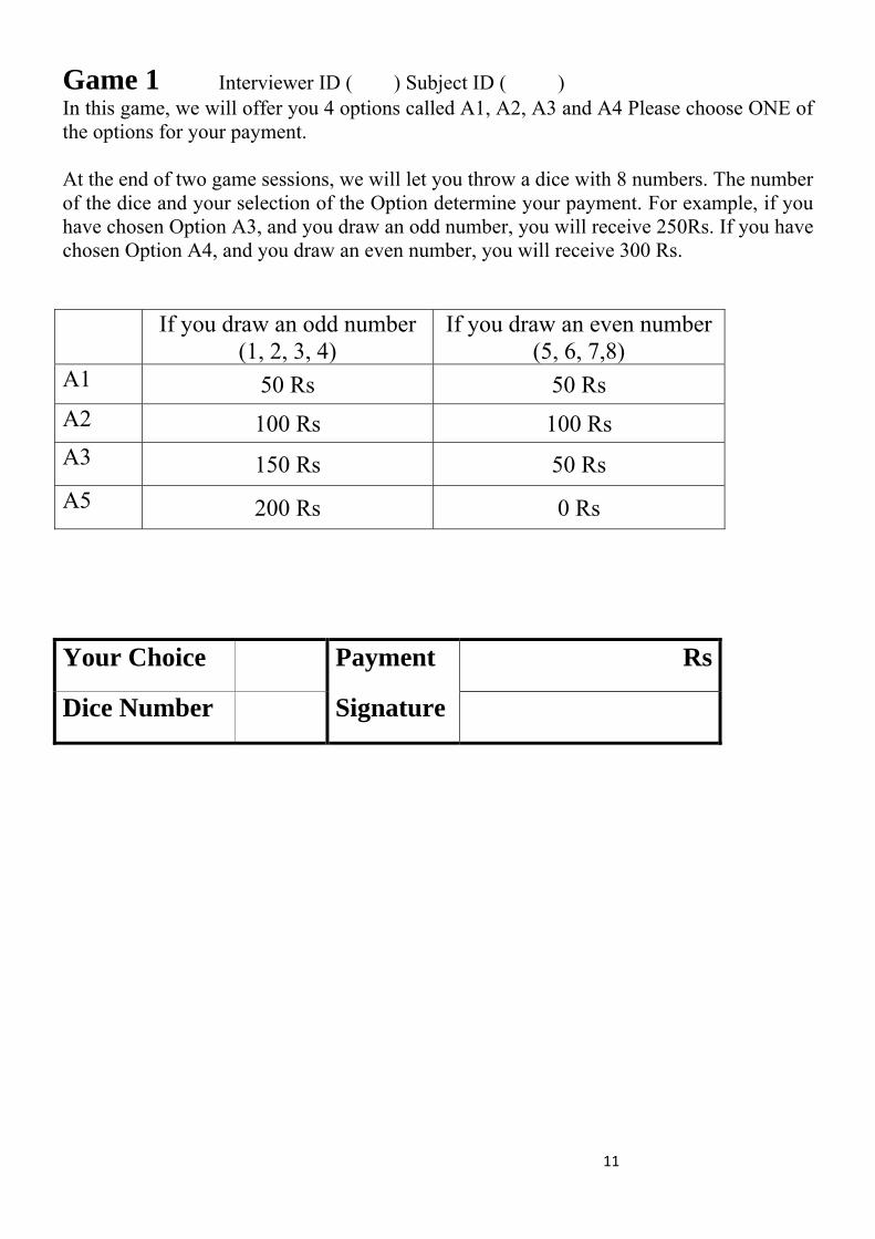
  11 

Game 1 Interviewer ID ( ) Subject ID ( ) In this game, we will offer you 4 options called A1, A2, A3 and A4 Please choose ONE of the options for your payment. At the end of two game sessions, we will let you throw a dice with 8 numbers. The number of the dice and your selection of the Option determine your payment. For example, if you have chosen Option A3, and you draw an odd number, you will receive 250Rs. If you have chosen Option A4, and you draw an even number, you will receive 300 Rs.

If you draw an odd number

(1, 2, 3, 4) If you draw an even number

(5, 6, 7,8) A1 50 Rs 50 Rs

A2 100 Rs 100 Rs

A3 150 Rs 50 Rs

A5 200 Rs 0 Rs

Your Choice Payment Rs

Dice Number Signature

D. Pictures

Figure 7: Weather station

Figure 8: Thermometer

Figure 9: Rain gauge

83

Reference

Alderman, H., Haque, T. (2007) Insurance against Covariate Shocks: The Role of Index-Based Insurance in Social Protection in Low-Income Countries, World Bank.

Barnett, B., Mahul, O. (2007) �Weather Index Insurance for Agriculture and Rural Areasin Lower Income Countries,�American Journal of Agricultural Economics, 89(5): 1241-1247.

Barnett, B., Barrett, C., Skees, J. (2007) �Poverty Traps and Index-Based Risk TransferProducts,�World Development, 36(10): 1766-1785.

Besley, T. (1995) �Nonmarket Institutions for Credit and Risk Sharing in Low-IncomeCountries,�Journal of Economic Perspectives, 9(3): 115�127.

Binswanger, H. P. (1980) �Attitudes Toward Risk: Theoretical Implications of an Exper-iment in Rural India,�American Journal of Agricultural Economics, 62(3): 395-407.

Cai, J. (2012) �Social Networks and the Development of Insurance Markets: Evidencefrom Randomized Experiments in China,�mimeo.

Carter, M., R. (2011) �Innovations for Managing Basis Risk under Index Insurance forSmall Farm Agriculture,�FERDI Policy Brief No.41

Carter, M., R. (2012) �Designed for Development Impact: Next Generation of IndexInsurance for Smallholder Farmers� In Churchill, C., Matul, M. Eds, Protecting the Poor:Microinsurance Compendium, Vol II. Chapter 11, Geneva, ILO.

Carter, M. R., Cheng, L., Sarris, A. (2011) �The Impact of Interlinked Index Insuranceand Credit Contracts on Financial Market Deepening and Small Farm Productivity,�mimeo.

Chantarat, S., Barrett, C.B., Mude, A. G., Turvey C. (2007) �Using Weather IndexInsurance to Improve Drought Response for Famine Prevention,�American Journal of Agri-cultural Economics, 89(5): 1262�1268.

Chen, K. Z., Liu, Y., Hill, R., Xiao, C., Liu, L. (2012) �Can We Relax Liquidity Con-straints on Microinsurance Demand? Piloting an Innovative Design for Agricultural Insur-ance,�Technical Report, Microinsurance Innovation Facility (Geneva, ILO).

Chuang, Y., Schechter, L. (2013) �Stability of Experimental and Survey Measures ofSocial, Risk, and Time Preferences Over Multiple Years,�Working Paper.

Clarke, D. J. (2011) �A Theory of Rational Demand for Index Insurance,�Oxford Uni-versity Department of Economics Discussion Paper 572.

Clarke, D., J. Mahul, O., Rao, K. N., Verma, N. (2011) �Weather Based Crop Insurancein India,�World Bank Policy Research Working Paper 5985.

84

Clarke, D. J. Das, N., de Nicola, F., Hill, R. V. Kumar, N., Metha, P. (2012) �The Valueof Customized Insurance for Farmers in Rural Bangladesh,�IFPRI Discussion Paper 01202.

Cole, S., Giné, X., Tobacman, J., Topalova, P., Townsend, R., Vickery, J. (2013). �Bar-riers to Household Risk Management: Evidence from India,�American Economic Journal:Applied Economics, 5(1): 104�135.

De Bock, O, Gelade, W., (2012) �The Demand for Microinsurance: A Literature Review�Research Paper No.26, Microinsurance Innovation Facility, Geneva, ILO.

De Janvry, A., Dequiedt, V., Sadoulet, E. (2013) �The Demand for Insurance againstCommon Shocks,�Journal of Development Economics.

Delavande, A., Giné, X., McKenzie, D. (2011a) �Measuring Subjective Expectationsin Developing Countries: A Critical Review and New Evidence,� Journal of DevelopmentEconomics, 94(2): 151�163.

Delavande, A., Giné, X., McKenzie, D. (2011b) �Eliciting Probabilistic Expectations withVisual Aids in Developing Countries: How Sensitive Are Answers to Variations in ElicitationDesign?�Journal of Applied Econometrics, 26(3): 479-497.

De Nicola, F. (2012) �The Impact of Weather Insurance on Consumption, Investmentand Welfare,�mimeo.

Dercon, S., Kirchberger, M., Gunning, J. W., Platteau, J-P., (2008) �Literature Reviewon Microinsurance�Research Paper No.1, Microinsurance Innovation Facility (Geneva, ILO).

Doherty, N., Shlesinger, H. (1990) �Rational Insurance Purchasing: Consideration ofContract Nonperformance,�Quarterly Journal of Economics, 55(1), 243-53.

Elabed, G., Bellemare, M. F.., Carter, R. M., Guirkinger, C. (2013) �Managing BasisRisk with Multiscale Index Insurance,�Agricultural Economics, 44, 419-431.

Fisher, M., Eitzinger, A, Nieto, J. D., Cook, S., Läderach, P., (2013) �Index WeatherInsurance for Smallholder Farmers: Who Takes the Risk?,�The Challenges of Index-BasedInsurance for Food Security in Developing Countries, European Commission.

Fuchs, A., Wol¤, H. (2011) �Concept and Unintended Consequences of Weather IndexInsurance: The Case of Mexico,�American Journal of Agricultural Economics, 93(2) Pro-ceedings, 505�511.

Galarza, F. B, Carter, M. R. (2010) �Risk Preferences and Demand for Insurance inPeru: A Field Experiment,�2010 Annual Meeting of Agricultural and Applied EconomicsAssociation.

Gallagher, J.. (2012) �Learning about an Infrequent Event: Evidence from Flood Insur-ance Take-up in the US,�mimeo.

85

Giné, X., Townsend, R., Vickery, J. (2008) �Patterns of Rainfall Insurance Participationin Rural India,�World Bank Economic Review, 22(3): 539-566.

Giné, X., Yang, D. (2009) �Insurance, Credit, and Technology Adoption: Field Experi-mental Evidence from Malawi,�Journal of Development Economics, 89(1): 1-11.

Goodwin, B. (1993) �An Empirical Analysis of the Demand for Multiple Peril CropInsurance,�American Journal of Agricultural Economics, 75: 425-434.

Hansen, L. P., (1982) �Large Sample Properties of Generalized Method of MomentsEstimators,�Econometrica, 50(4): 1029-1054.

Hazell, P. (2003) �Potential Role for Insurance in Managing Catastrophic Risk in De-veloping Countries,�Proceedings of the World Bank Conference on Financing the Risks ofNatural Disasters, June 2�3, 2003.

Hayashi, F. (2000) Econometrics, Princeton University Press.

Heckman, J. (1979) �Sample Selection Bias as a Speci�cation Error,� Econometrica,47(1): 153-61.

Janzen, S. A., Carter, M. R. (2013) �The Impact of Microinsurance on ConsumptionSmoothing and Asset Protection: Evidence from a Drought in Kenya,�mimeo.

Karlan, D., Osei, R., Osei-Akoto, I., Udry, C. (2012) �Agricultural Decisions After Re-laxing Credit and Risk Constraints,�NBER Working Paper No.18463.

Kurosaki, T., Fafchamps, M. (2002) �Insurance Market E¢ ciency and Crop Choices inPakistan,�Journal of Development Economics, 67(2): 419-453.

Lilleor, H. B., Giné, X., Townsend, R., Vickery, J. (2005) �Weather Insurance in Semi-Arid India,�mimeo.

Ligon, E., Thomas, J. P., Worrall, T. (2002) �Informal Insurance Arrangements withLimited Commitment: Theory and Evidence from Village Economies,�Review of EconomicStudies, 69: 209-244

Ligon, E. (2008) �Risk Sharing,�In S.N. Durlauf, & L. E. Blume (Eds), The New PalgraveDictionary of Economics, Second Edition. Palgrave Macmillan.

Harrison, G. W. , List, J.A. (2004) �Field Experiments,�Journal of Economic Literature,42(4): 1009-1055.

Mahul, O., Wright, B.D. (2007) �Optimal Coverage for Incompletely Reliable Insurance,�Economics Letters, 95: 456-461.

Mahul, O., Wright, B.D. (2007) �Designing Optimal Crop Revenue Insurance,�AmericanJournal of Agricultural Economics, 85(3), 580-589.

86

Mahul, O., Wright, B.D. (2004) �Implications of Incomplete Performance for OptimalInsurance" Economica, 71, 661-670.

Matul, M., Dalal, A., De Bock, O., Gelade, W. (2013) �Why People Do Not Buy Mi-croinsurance and What Can We Do About It?�International Labour O¢ ce, MicroinsurancePaper No.20.

McCarthy, N. (2003) �Demand for Rainfall-Index Based Insurance: A Case Study fromMorocco,�EPTD Discussion Paper No.106.

Miranda, J. M., Glauber, J. (1997) �Systemic Risk, Reinsurance, and the Failure of CropInsurance Markets,�American Journal of Agricultural Economics, 79: 206�215.

Miura, K., Sakurai, T. (2012) �Who Purchases Weather Index Insurance? Results froma Field Experiment in Rural Zambia,�Journal of Rural Economics, Special Issue, 442�449(in Japanese).

Mobarak, A.M., Rosenzweig, M. (2012a) �Selling Formal Insurance to the InformallyInsured,�mimeo.

Mobarak, A.M., Rosenzweig, M. (2012b) �Informal Risk Sharing, Index Insurance andRisk -Taking in Developing Countries,�mimeo.

Morduch, J. (1994) �Poverty and Vulnerability,�American Economic Review, Papersand Proceedings, 84(2): 221-225.

Morduch, J. (1995) �Income Smoothing and Consumption Smoothing,�Journal of Eco-nomic Perspectives, 9(3): 103-114.

Morduch, J. (2006) �Micro-Insurance: The Next Revolution?� in A. Banerjee, R. Ben-abou, and D. Mookherjee (eds), What Have We Learned About Poverty? Oxford and NewYork: Oxford University Press.

Newey, W. K. , Powell, J. L. , Walker, J. R. (1990) �Semiparametric Estimation of Selec-tion Models: Some Empirical Results,�American Economic Review, Papers and Proceedings,Vol. 80, No.2 , 324-328

NSSO (National Sample Survey Organisation) (2006) �Household Ownership Holdings inIndia, 2003: NSS 59 Round (January�December 2003),�New Delhi: Government of India,Ministry of Statistics and Programme Implementation, NSSO, November 2006, Report No.491 (59/18.1/4).

Patrick, G.F. (1988) �Mallee wheat farmers�demand for crop and rainfall insurance,�Australian Journal of Agricultural Economics, 32, 1:37-49.

Rabin, M. (2000) �Risk Aversion and Expected-utility Theory: A Calibration Theorem,�Econometrica, 68(5): 1281-1292.

87

Ragoubi, N., Belekacem, L., Mimoun, A. B. (2013) �Rainfall-Index Insurance and Tech-nology Adoption: Evidence from Field Experiment in Tunisia,� Journal of InternationalDevelopment, 25: 660-673.

Rosenzweig, M., Binswanger, H. (1993) �Wealth, Weather Risk and the Composition andPro�tability of Agricultural Investments,�Economic Journal, 103, 56�78.

Sakurai, T. and Reardon, T. (1997) �Potential Demand for Drought Insurance in BurkinaFaso and Its Determinants,�American Journal of Agricultural Economics, 79: 1193-1207.

Skees, J., Gober, S., Varangis, R., Lester, R., Kalavakonda, V. (2001) �DevelopingRainfall-Based Index Insurance in Morocco,�World Bank Policy Research Working Paper,2577.

Skees, J., Varangis, P., Larson, D., Siegel, P. (2005) �Can Financial Markets be Tapped toHelp Poor People Cope with Weather Risks?�in S. Dercon (Eds), Insurance against Poverty,Oxford and New York: Oxford University Press.

Townsend, R.M. (1994) �Risk and Insurance in Village India,� Econometrica, 62(3):539-591.

Udry, C. (1994) �Risk and Insurance in a Rural Credit Market: An Empirical Investiga-tion in Northern Nigeria,�Review of Economic Studies, 61(3): 495-526.

Vella (1998) �Estimating Models with Sample Selection Bias: A Survey,� Journal ofHuman Resources, 33(1): 127-169.

Walker, T.S., Ryan, J.G. (1990) Village and Household Economies in India�s Semi-AridTropics, Johns Hopkins.

Wright, B., Hewitt, J.A. (1994) �All-Risk Crop Insurance: Lessons from Theory andExperience�in D. L. Hueth and W. Furtan (Eds), Economics of Agricultural Crop Insurance:Theory and Evidence, Springer.

88