essays in economic development and political economy

Essays in Economic Developmentand Political Economy

The Harvard community has made thisarticle openly available. Please share howthis access benefits you. Your story matters

Citation Neggers, Yusuf. 2016. Essays in Economic Development and PoliticalEconomy. Doctoral dissertation, Harvard University, Graduate Schoolof Arts & Sciences.

Citable link http://nrs.harvard.edu/urn-3:HUL.InstRepos:33493380

Terms of Use This article was downloaded from Harvard University’s DASHrepository, and is made available under the terms and conditionsapplicable to Other Posted Material, as set forth at http://nrs.harvard.edu/urn-3:HUL.InstRepos:dash.current.terms-of-use#LAA

http://osc.hul.harvard.edu/dash/open-access-feedback?handle=&title=Essays%20in%20Economic%20Development%20and%20Political%20Economy&community=1/1&collection=1/4927603&owningCollection1/4927603&harvardAuthors=fd28aa84b887d526b5001a35b7fe5166&departmentPublic%20Policy

http://nrs.harvard.edu/urn-3:HUL.InstRepos:33493380

http://nrs.harvard.edu/urn-3:HUL.InstRepos:dash.current.terms-of-use#LAA



Essays in Economic Development and PoliticalEconomy

A dissertation presented

by

Yusuf Neggers

to

The Department of Public Policy

in partial fulfillment of the requirements

for the degree of

Doctor of Philosophy

in the subject of

Public Policy

Harvard University

Cambridge, Massachusetts

April 2016

Dissertation Advisor:Professor Rohini Pande

Author:Yusuf Neggers

Essays in Economic Development and Political Economy

Abstract

The three chapters in this dissertation examine aspects of the relationships between trans-

parency, government accountability, and the quality of public services. In the first chapter,

I ask how ethnic diversity, or lack thereof, among polling station officials affects voting

outcomes. I exploit a natural experiment occurring in the 2014 parliamentary elections in

India, where the government mandated the random assignment of state employees to the

teams that managed polling stations on election day. I find that the presence of officers of

minority identities within teams led to significant shifts in vote share toward the political

parties associated with these groups. Results suggest that the magnitude of these effects

is large enough to be relevant to election outcomes. Using large-scale survey experiments,

I provide evidence of own-group favoritism in polling personnel and identify the process

of voter identity verification as an important channel through which voting outcomes are

impacted.

The second chapter examines whether electronic procurement (e-procurement), which

increases access to information and reduces personal interactions with potentially corrupt

officials, improves procurement outcomes in India and Indonesia. We find no evidence

of reduced prices but do find that e-procurement leads to quality improvements in both

countries. Regions with e-procurement are also more likely to have winners come from

outside the region. On net, the results suggest that e-procurement facilitates entry from

higher quality contractors.

The third chapter studies the effects of the enactment across U.S. states of open meetings

laws which ostensibly increase the public availability of information on legislator behavior.

iii

As recent work shows that increased remoteness of capital cities in U.S. states is strongly as-

sociated with reduced accountability and worse government performance, I also investigate

how the impacts of open meetings vary with state capital isolation. I find that open meetings

increase spending on public goods and heighten confidence in state government on average.

Heterogeneous impacts on incumbent vote share suggest that at both low and high levels

of initial accountability, open meetings provide citizens with additional information that

influences voting decisions.

iv

Contents

Abstract . . . . . . . . . . . . . . . . . . . . . . . . . . . . . . . . . . . . . . . . . . . . iiiAcknowledgments . . . . . . . . . . . . . . . . . . . . . . . . . . . . . . . . . . . . . x

Introduction 1

1 Enfranchising Your Own? Experimental Evidence on Polling Officer Identity andElectoral Outcomes in India 71.1 Introduction . . . . . . . . . . . . . . . . . . . . . . . . . . . . . . . . . . . . . . 71.2 Background . . . . . . . . . . . . . . . . . . . . . . . . . . . . . . . . . . . . . . 131.3 Team composition: channels of impact . . . . . . . . . . . . . . . . . . . . . . . 181.4 Data . . . . . . . . . . . . . . . . . . . . . . . . . . . . . . . . . . . . . . . . . . 231.5 Reduced-form impacts on voting outcomes . . . . . . . . . . . . . . . . . . . . 291.6 Channel of impact: officer bias in discretionary decisions . . . . . . . . . . . . 331.7 Alternative explanations . . . . . . . . . . . . . . . . . . . . . . . . . . . . . . . 471.8 Conclusion . . . . . . . . . . . . . . . . . . . . . . . . . . . . . . . . . . . . . . . 48

2 Can Electronic Procurement Improve Infrastructure Provision? Evidence fromPublic Works in India and Indonesia 522.1 Introduction . . . . . . . . . . . . . . . . . . . . . . . . . . . . . . . . . . . . . . 522.2 Background . . . . . . . . . . . . . . . . . . . . . . . . . . . . . . . . . . . . . . 572.3 Data and empirical strategy . . . . . . . . . . . . . . . . . . . . . . . . . . . . . 652.4 Results . . . . . . . . . . . . . . . . . . . . . . . . . . . . . . . . . . . . . . . . . 722.5 Conclusion . . . . . . . . . . . . . . . . . . . . . . . . . . . . . . . . . . . . . . . 82

3 Out of Sight, Out of Mind: Impacts of Open Meetings in U.S. State Legislatures 863.1 Introduction . . . . . . . . . . . . . . . . . . . . . . . . . . . . . . . . . . . . . . 863.2 Conceptual framework . . . . . . . . . . . . . . . . . . . . . . . . . . . . . . . . 893.3 Background and data . . . . . . . . . . . . . . . . . . . . . . . . . . . . . . . . . 913.4 Identification . . . . . . . . . . . . . . . . . . . . . . . . . . . . . . . . . . . . . . 983.5 Results . . . . . . . . . . . . . . . . . . . . . . . . . . . . . . . . . . . . . . . . . 993.6 Conclusion . . . . . . . . . . . . . . . . . . . . . . . . . . . . . . . . . . . . . . . 107

v

References 111

Appendix A Appendix to Chapter 1 119A.1 Survey sampling . . . . . . . . . . . . . . . . . . . . . . . . . . . . . . . . . . . 119A.2 Vignette experiment names and list experiments prompt . . . . . . . . . . . . 121A.3 Counterfactual calculation details . . . . . . . . . . . . . . . . . . . . . . . . . 121A.4 Supplemental figures and tables . . . . . . . . . . . . . . . . . . . . . . . . . . 123

Appendix B Appendix to Chapter 2 132

Appendix C Appendix to Chapter 3 134

vi

List of Tables

1.1 Randomization check . . . . . . . . . . . . . . . . . . . . . . . . . . . . . . . . . 281.2 Impacts of randomized officer team composition on voting outcomes . . . . 301.3 Vignette experiment: own-type bias in officer assessment of voters . . . . . . 351.4 List experiments: biased officer behavior on election day . . . . . . . . . . . 391.5 Overall polling station management . . . . . . . . . . . . . . . . . . . . . . . . 411.6 Identity verification experience of potential voters . . . . . . . . . . . . . . . . 431.7 Heterogeneity in effects of team composition by voter identity card coverage 451.8 Variation in other officer characteristics by Muslim/Yadav identity . . . . . . 481.9 Changes in election outcomes under alternative officer assignment mechanisms 50

2.1 Summary statistics . . . . . . . . . . . . . . . . . . . . . . . . . . . . . . . . . . 692.2 Budget impact . . . . . . . . . . . . . . . . . . . . . . . . . . . . . . . . . . . . . 732.3 Contract process . . . . . . . . . . . . . . . . . . . . . . . . . . . . . . . . . . . . 752.4 Prices and project execution . . . . . . . . . . . . . . . . . . . . . . . . . . . . . 782.5 Two-stage contractor fixed effect regressions . . . . . . . . . . . . . . . . . . . 83

3.1 Summary statistics . . . . . . . . . . . . . . . . . . . . . . . . . . . . . . . . . . 953.2 Legislative activity . . . . . . . . . . . . . . . . . . . . . . . . . . . . . . . . . . 1003.3 State direct expenditure . . . . . . . . . . . . . . . . . . . . . . . . . . . . . . . 1023.4 Confidence in state government . . . . . . . . . . . . . . . . . . . . . . . . . . . 1043.5 Voting outcomes . . . . . . . . . . . . . . . . . . . . . . . . . . . . . . . . . . . 106

A.1 Randomization check - spatial characteristics . . . . . . . . . . . . . . . . . . . 125A.2 Cross-position balance . . . . . . . . . . . . . . . . . . . . . . . . . . . . . . . . 126A.3 Position- and number-specific impacts on voting outcomes . . . . . . . . . . . 127A.4 Heterogeneity in impacts of team composition by electorate composition . . 128A.5 Cross-station spillovers - extended range . . . . . . . . . . . . . . . . . . . . . 129A.6 Type-specific impacts of officer identity on voting outcomes . . . . . . . . . . 130A.7 Cross-election impacts of randomized team composition on voting outcomes 131

B.1 Differential initial trends check . . . . . . . . . . . . . . . . . . . . . . . . . . . 133

vii

C.1 Candidate entry . . . . . . . . . . . . . . . . . . . . . . . . . . . . . . . . . . . . 135

viii

List of Figures

1.1 Election administration difficulties by country . . . . . . . . . . . . . . . . . . 91.2 Polling station distribution across example parliamentary constituency . . . 151.3 Variation in officer team composition across polling stations . . . . . . . . . . 221.4 Empirical distribution of coalition vote share margins by team composition . 291.5 Own-type bias in officer assessment of voters . . . . . . . . . . . . . . . . . . . 361.6 Heterogeneity by voter identity card coverage in impact of team composition 46

2.1 Number of contracts by numbers of technical disqualifications and bidders . 592.2 E-procurement adoption - India . . . . . . . . . . . . . . . . . . . . . . . . . . . 602.3 E-procurement adoption - Indonesia . . . . . . . . . . . . . . . . . . . . . . . . 63

3.1 Timing of open meetings adoption across states . . . . . . . . . . . . . . . . . 923.2 Distribution of state capital isolation . . . . . . . . . . . . . . . . . . . . . . . . 933.3 Event study of legislative and expenditure outcomes . . . . . . . . . . . . . . 1083.4 Event study of election outcomes . . . . . . . . . . . . . . . . . . . . . . . . . . 109

A.1 Example of polling officer team during election day proceedings . . . . . . . 123A.2 Example of government-issued voter identity card . . . . . . . . . . . . . . . . 123A.3 Example of neighboring polling stations in close proximity . . . . . . . . . . 124A.4 Cumulative distribution function of coalition vote share margins . . . . . . . 124

ix

Acknowledgments

I thank the many people and institutions who have provided me guidance and support over

the last six years.

For superb mentoring and patience, my advisors: Rohini Pande, Alberto Alesina, Rema

Hanna, and Andrei Shleifer.

For comments, advice, friendship, and moral support: Michael Callen, Vanessa Cheng,

Eric Dodge, Dan Fehder, Benjamin Feigenberg, Nilesh Fernando, Tye Greene, Alicia Harley,

Ben Iobst, Simon Jäger, Leandra King, Horacio Larreguy, Patrick Mayne, Peter Murphy,

Daria Pelech, Swapna Reddy, Natalia Rigol, Monica Singhal, Charles Stewart, Samuel Stolper,

and Jacob Wallace.

For financial support: National Science Foundation, J-PAL Governance Initiative, Har-

vard Sustainability Science Program, Harvard Perini and Cunningham Dissertation Fellow-

ship for International Development, Harvard Lab for Economic Applications and Policy,

Weiss Family Program Fund, Pershing Square Venture Fund for Research on the Foundations

of Human Behavior, Harvard South Asia Institute, and Harvard Institute for Quantitative

Social Science.

x

To Joseph, Yasmin, Xavira, and Khaled.

xi

Introduction

In the first chapter of this dissertation, I ask how ethnic diversity, or lack thereof, in the

teams of officers that manage polling stations on election day affects voting outcomes. I take

advantage of a natural experiment in the Indian electoral setting in which government em-

ployees were randomly assigned to teams of polling station officials, generating exogenous

variation in team composition in terms of religious and caste identity, both of which are

strongly connected with political affiliation.

I use detailed polling station location information and unique officer assignment data

for two districts in the state of Bihar covering more than 5.6 million registered voters in the

2014 national elections. I identify both direct effects within stations and spillover effects

across stations of changes in team religious and caste composition on voting outcomes,

demonstrating that the direct effects alone would be a biased estimate of the total impact.

To go further and shed light on underlying mechanisms, I embedded experiments in

surveys of individuals randomly selected from the same populations of election officers

and registered voters that were exposed to the election policy experiment. These data allow

me to test for election officer bias and determine whether such bias leads to differential

treatment of voters on election day.

I find strong evidence that own-group bias in election officers exists and influences the

treatment of potential voters on election day. Using a vignette experiment in which polling

station officers assess the likelihood that a hypothetical individual would be allowed to

vote, I find that officers are significantly more likely to favorably assess the individual’s

qualification to vote when they are of the same religious/caste-group type. In addition,

1

the results of list experiments show that election officers treated potential voters differently

based on religion/caste and explicitly attempted to influence citizens’ voting behavior.

Consistent with the experimental results, I also find that minority potential voters at

polling stations with no minority officers are on average significantly less satisfied with their

overall polling station experience and less likely to be able to vote than are non-minority

individuals. These effects disappear, however, at polling stations with minority officers

present or when individuals possess a government-issued voter identity card, a method of

identification which reduces officer discretion in determining voter eligibility. Furthermore,

I confirm that the polling-station-level effects of team composition on voting outcomes are

concentrated in areas with lower voter identity card coverage.

Counterfactual calculations indicate that the combined direct and indirect team com-

position effects are large enough to influence the outcomes of elections. Given that the

two major political coalitions in this setting strongly differ in their propensities to field

Muslim candidates, this also suggests that changes in officer team assignment could lead to

significant shifts in the Muslim proportion of officeholders.

Fair and well-functioning elections are critical to maintaining the responsiveness of

elected officials to citizens in democracies. While the related literature on election reforms

has focused in large part on the benefits of advances in monitoring and voting technology,

this paper is to my knowledge the first to provide rigorous evidence of the remaining impor-

tance of the identities of local-level election personnel. Indian elections are technologically

advanced and their administration is highly regulated, indicating that bias in discretionary

decision making of polling station officers can undermine the quality of service provision

even at the present frontier of election practice.

The second chapter examines the impacts of the transition by developing country gov-

ernments to electronic procurement (e-procurement) of goods and services. E-procurement

can potentially address three common concerns with manual procurement practices: lack of

access to bid information, collusion among bidders, and corruption. However, it is plausible

that in low income settings, where information technology coverage and other aspects of

2

state capacity remain low, e-procurement can only effect limited change and can potentially

make things worse.

We examine the impact of electronic procurement on public works projects in two large

emerging economies: India and Indonesia. In India, we examine procurement practices for

a federally funded rural road construction program which is implemented by state road

departments. In Indonesia, we examine contract data from the national Ministry of Public

Works for both construction and consulting (e.g., engineering management and design)

contracts each year. The gradual roll-out of e-procurement (at the state-level in India and

province-level in Indonesia) allows for a difference-in-differences strategy: We compare

outcomes in states/provinces before and after the adoption of e-procurement, as well as in

those continuing under manual procurement practices, allowing us to quantify the benefits

or costs of the practice in both countries.

For both countries, we obtained administrative data on the complete universe of contracts

from before and after e-procurement by scraping publicly available information from

respective government websites. In addition, in India, we hand collected bidding data on

tenders for four states which we use to supplement the administrative data.

We first show that, in both India and Indonesia, e-procurement increases the probability

that the winning bidder comes from outside the region where the contract takes place.

This is consistent with e-procurement decreasing the costs of submitting bids for those not

physically present. We next examine the impact on the ultimate outcomes of interest: price,

quality of construction, and timeliness.

We find no systematic evidence that electronic procurement lowers prices paid by

the government. In contrast, e-procurement led to quality improvements, albeit along

different dimensions in the two countries. A first measure of quality is time-overrun in

project completion. In India, we observe no statistically significant changes in late works,

while in Indonesia these declines are large and significant. A separate indicator of quality,

only available for India, is an independent audit report on construction quality, which

was conducted identically in roads completed under both e-procurement and traditional

3

procurement. According to this measure, we find that e-procurement leads to higher quality

roads.

We then explore the degree to which the results are driven by improving outcomes

among already winning bidders, as opposed to changing who wins. We find that after

e-procurement, winning contractors in India tend to be those who have higher quality on av-

erage. In Indonesia, we find evidence that those contractors who win after e-procurement are

systematically less likely to be late. This suggests that a key mechanism for e-procurement is

allowing higher quality contractors to enter and win projects, rather than simply encouraging

better performance from an existing set of contractors.

The fact that we observe changes on the quality margin, and that it occurs through

changing which contractors win rather than the performance of a given set of winning

contracts, suggests that the system prior to e-procurement was not necessarily selecting the

most efficient firms, and that e-procurement may have improved efficiency even if it did

not necessarily lower prices paid. It also suggests that the practice of giving contracts to

the lowest price bidder likely contributed to greater inefficiencies on the quality margin.

Overall, our findings provide qualified support to the view that e-governance can improve

the provision of public services.

The third chapter provides empirical evidence on the effects of increased transparency

of the actions of elected representatives in the U.S. state legislative setting. Increases in

institutional transparency in democracies are commonly assumed to improve outcomes

of policy making. While proponents of greater transparency emphasize the benefits of

increased accountability and responsiveness of elected representatives, theory suggests that

greater transparency need not lead to beneficial consequences for the general public. For

example, it may be that, in contexts where it is difficult for the public to evaluate fully the

consequences of representatives’ choices, increasing observability of the actions themselves

may increase the incentives of representatives to disregard valuable private information

when choosing what to do. Given the theoretical uncertainty, an empirical investigation

is valuable in helping to improve our understanding of which of the potential forces are

4

dominant in U.S. state legislatures.

I exploit variation in the timing of enactment of open meetings laws across U.S. states

and employ a difference-in-differences estimation strategy. I examine the impact of open

meetings on the total numbers of bills introduced and enacted and on the timeliness with

which the state budget, arguably the most important piece of legislative output, is delivered.

As a more direct measure of whether legislators are incentivized to take actions with

important economic impacts, state government expenditure is considered as an outcome. I

finally examine how open meetings influence citizens’ perceptions of government and their

behavior in elections to state legislatures.

In addition to considering the average impacts of open meetings on these outcomes, I

investigate how the effects are mediated by the level of geographic isolation of the state

legislature from its constituents, which recent work has shown to be robustly associated

with weaker accountability and worse government performance. The effects of increasing

transparency through open meetings may then differ in the isolation of the state government,

due to differences across states both in the baseline level of quality of government and in the

effective magnitude of the change in public informedness associated with open meetings.

I find that open meetings decrease legislative enactments, but do not impact the number

of bills introduced or timeliness of budgets on average. Results suggest that open meetings

significantly increase expenditure on public goods, and that these expenditure effects are

concentrated in areas with greater state capital isolation, where government spending on

public goods is lower to begin with.

Open meetings also shift citizens’ perceptions of state government, such that in national-

level Gallup surveys they are significantly more likely to express at least moderate confidence

in the government on average. An examination of heterogeneity in impacts by capital

isolation shows that the effects are driven by gains in low isolation areas. In states with more

isolated capitals, open meetings actually increase the proportion of respondents choosing

the lowest possible measure of confidence. Mirroring this pattern, I observe significant

differences in the impact of open meetings on voting outcomes by the isolation of the capital.

5

Whereas incumbents in low isolation locations see their vote shares increase with open

meetings, those where the capital is more remote experience a decrease in vote share.

The findings of this chapter suggest that open meetings in the U.S. state legislative

setting are on average beneficial. Expenditure on public goods increases, concentrated

in areas where spending of this type is the lowest to start. Additionally, citizens express

greater confidence in the ability of state governments. The results also indicate that, even in

environments with low initial levels of accountability, open meetings lead to shifts in voters’

information and that they respond to its content. That is, weak transmission mechanisms to

the public or low uptake by citizens do not appear to be binding constraints which prevent

increased accessibility of information about legislator behavior from producing downstream

effects.

6

Chapter 1

Enfranchising Your Own?

Experimental Evidence on Polling

Officer Identity and Electoral

Outcomes in India

1.1 Introduction

Electoral malpractice and election day violence are common problems across the world,

as the most recent round of the World Values Survey shows.1 Figure 1.1 shows that at

least twenty-five percent of respondents in more than one half of survey countries indicate

that violence at the polling station is often a problem, and in nearly three quarters of

countries that election officials are often unfair. The provision of well-functioning elections

constitutes a critical public service. The ability of a country’s citizens to cast votes in a free

and fair setting is desirable in its own right, but is additionally important to the extent

1Round 6 was administered to representative samples of individuals across sixty countries between 2010and 2014, but in only forty-two were election-related questions asked. This round was the first to include suchquestions.

7

that it increases the accountability of elected officials, with subsequent impacts on policy

decisions and citizen welfare (Besley and Case 1993, Maskin and Tirole 2004).

Election management and voting technology vary widely across countries, including a

fundamental aspect of electoral administration, the staffing of polling stations on election

day. Volunteers manage polling stations in the United States, while in Argentina randomly

selected citizens work as polling station officials within their own municipalities. In India

polling officials are randomly drawn from pools of government employees, and in Kenya

polling officers are temporary, paid positions staffed through an open application process.

Given the variety in election administration across countries and the frequent dissatisfaction

of citizens with elections, there is clear need for causal evidence on what works in election

reforms, particularly in relation to personnel management.

In this paper, I ask how ethnic diversity, or lack thereof, in the teams of officers that

manage polling stations on election day affects voting outcomes. I take advantage of a

natural experiment in the Indian electoral setting in which government employees were

randomly assigned to teams of polling station officials. The government’s assignment

method generates random variation in team composition in terms of religious and caste

identity, both of which are strongly connected with political affiliation. Largely in opposition

to upper-caste Hindu influence, Muslims and Yadavs (a low-caste Hindu group) formed a

political alliance in the state of Bihar in the mid-1990s, and this coalition remained operative

in the most recent 2014 national elections.2 The teams of officers I study contained at least

one Muslim or Yadav approximately one third of the time, allowing me to identify the

causal impacts of shifting from a “homogeneous” to “mixed” team of officers at a polling

station.3

The random assignment circumvents otherwise confounding issues of selection in

election officer placement at polling stations. A government may assign election personnel

2Wittsoe (2013) provides a detailed account of the state of the alliance over time.

3Due to the low proportions of Muslims and Yadavs among officers, teams that are fully Muslim/Yadav arenot observed in my sample.

8

Algeria

Azerbaijan

Argentina

Australia

Brazil

Chile

Taiwan

Colombia

Ecuador

Estonia

Georgia

Palestine

Germany

Ghana

Hong Kong

India

Iraq

Kazakhstan

Jordan

Kuwait

Kyrgyzstan

Lebanon

Libya

Malaysia

Mexico

Netherlands

Nigeria

Pakistan

Peru

Philippines

Poland

Romania

Rwanda

Singapore

South Africa

Zimbabwe

Thailand

Tunisia

Ukraine

Egypt

Uruguay

Yemen

0.2

.4.6

.8O

ften

viol

ence

at p

olls

0 .2 .4 .6 .8Election officials often unfair

Algeria

Azerbaijan

Argentina

Australia

Brazil

ChileTaiwan

Colombia

Ecuador

Estonia

Georgia

Palestine

Germany

Ghana

Hong Kong

India

Iraq

KazakhstanJordan

Kuwait

KyrgyzstanLebanon

Libya

Malaysia

Mexico

Netherlands

Nigeria

Pakistan

Peru

Philippines

Poland

Romania

Rwanda

Singapore

South Africa

Zimbabwe

Thailand

Tunisia

Ukraine

Egypt

Uruguay

Yemen

0.2

.4.6

.8V

otes

ofte

n co

unte

d un

fairl

y

0 .2 .4 .6 .8Election officials often unfair

Notes: Measures computed using World Values Survey Wave 6 (2010-2014). “Election officials often unfair” isthe weighted percentage of respondents in each country, when asked “In your view, how often do the followingthings occur in this country’s elections?”, answering “Not at all often” or “Not often” to “Election officials arefair”, against the alternatives of “Very often”, “Fairly often”, or “Don’t know/Not answer”. “Often violence atpolls” is the percentage answering “Very often” or “Fairly often” to “Voters are threatened with violence at thepolls.” “Votes often counted unfairly” is the percentage answering “Not at all often” or “Not often” to “Votesare counted fairly.”

Figure 1.1: Election administration difficulties by country

9

with greater experience to manage more troubled locations in an effort to maintain neutrality.

Alternatively, the ruling party may station supporters as officers in strategically important

areas to influence outcomes in their favor. In either case, the assignment of officers would

be endogenous to voting behavior. Conditional on the integrity of the randomization, which

I test and confirm, the setting considered in this paper is not subject to issues of this type.

An additional benefit of the study context is that the polling officer assignment policy had

already been in place statewide for a decade at the time of the election under consideration,

eliminating concerns that the estimated impacts reflect only partial equilibrium effects that

may disappear once the policy is brought to full scale or as the government and political

parties adjust to the change over time (Acemoglu 2010, Svensson and Yanagizawa-Drott

2012).

I study two districts in Bihar covering more than 5.6 million registered voters across

5,561 polling stations for the 2014 national elections. Using detailed polling station location

information and unique officer assignment data, I identify both the direct effects within

stations and the spillover effects across stations of changes in team religious and caste

composition on voting outcomes. The omission of these cross-station effects could potentially

bias the estimates of overall impact.

To go further and shed light on underlying mechanisms, I embedded experiments in

surveys of individuals randomly selected from the same populations of election officers

and potential voters that were exposed to the election policy experiment.4 These data allow

me to test for election officer bias and determine whether such bias leads to differential

treatment of voters on election day.

This paper has three main results. First, I find that changes in team composition affect

voting both within and across polling stations. The average vote share margin between the

two major political coalitions is reduced on average by 2.3 percentage points, or 12.7 percent,

when the officer team at a given polling station is mixed. This shift is driven by a significant

4“Potential voter” refers to registered voters who went to the polling station on election day with theintention of voting.

10

4.6 percent increase in votes for the minority-oriented coalition and a 4.1 percent decrease

in votes for the non-minority coalition. In addition, I find that having a neighboring station

that is mixed rather than homogeneous decreases the vote share margin by an average of 2.6

percentage points, demonstrating that the direct effects alone would be an underestimate of

the total impact.

Second, I find strong evidence that own-group bias in election officers exists and in-

fluences the treatment of potential voters on election day. I measure bias using a vignette

experiment in which polling station officers assess the likelihood that a hypothetical in-

dividual would be allowed to vote, based on a description where all information is held

constant across respondents with the exception of the individual’s name, which is varied

randomly. Officers are 10 percentage points, or 25 percent, more likely to favorably assess

the individual’s qualification to vote when they are of the same religious/caste-group type.

In addition, I find using separate list experiments that approximately 20 to 25 percent of

officer and potential voter respondents agree that election officers treated potential voters

differently based on religion/caste on election day, and roughly 5 to 10 percent that officers

explicitly attempted to influence individuals’ voting behavior.

Consistent with the experimental results, I find that Muslim/Yadav potential voters

at polling stations with no minority officers are on average significantly less satisfied

with their overall polling station experience and less likely to be able to vote than are

non-Muslim/Yadav individuals. These effects disappear, however, at mixed team polling

stations or when individuals possess a government-issued voter identity card, a method of

identification which reduces officer discretion in determining voter eligibility. Furthermore,

I confirm that the previously identified polling-station-level effects of team composition on

voting outcomes are concentrated in areas with lower voter identity card coverage. Taken

together my results suggest that religious/caste diversity within officer teams and the

reduction of the scope for discretion in officer duties function as substitutes in improving

the impartiality of election proceedings.

Third, I ask whether the combined direct and indirect team composition effects are large

11

enough to influence the outcomes of elections. Under reasonable assumptions, estimates

from counterfactual calculations indicate that alternative officer assignment mechanisms

would have changed the identity of the winning coalition in approximately 5 to 15 percent

of races in the most recent national and state elections in Bihar. Given that the two major

political coalitions strongly differ in their propensities to field Muslim candidates, these

changes in election outcomes would have led to approximately a 25 percent increase in

Muslim officeholders. Recent work finds that in India the election of Muslim legislators

significantly improves child health and education outcomes (Bhalotra et al. 2014), further

suggesting how officer team composition can have downstream effects on citizen well-being.

This paper complements the literature examining technology-centered approaches to

strengthening elections. While technological innovations in the election setting have been

shown to significantly impact electoral fraud (Callen et al. 2015), voter turnout (Marx et al.

2014), and even subsequent public service delivery and health (Fujiwara 2015), less progress

has been made in understanding, holding the electoral setting otherwise constant, how the

identities of election personnel may still matter.

My results additionally relate to work which finds that election observers reduce fraud

at their posted polling stations when they represent non-politically affiliated international

or domestic organizations (Hyde 2007, Ichino and Schündlen 2012), but may introduce

additional bias when they themselves have partisan preferences (Casas et al. 2014). While

this literature considers individuals external to the government who are explicitly tasked

with monitoring polling stations, I focus on the government agents responsible for managing

election proceedings themselves.

This paper also contributes to the body of research studying the negative impacts of

ethnic fractionalization on government decision making and the provision of public goods

(Easterly and Levine 1997, Alesina et al. 1999, Miguel 2004, Miguel and Gugerty 2005,

Shayo and Zusman 2011). I provide micro-econometric evidence on an additional area, the

administration of elections, in which heterogeneity in the ethnic composition of a population

can lead to adverse effects on the quality of public service provision.

12

Finally, the implications of my work are also relevant to a literature examining potential

discrimination against blacks and hispanics in the American electoral system. Recent

research suggests that minorities in the US have different procedural experiences at polling

stations on election day (Ansolabehere 2009, Atkeson et al. 2010, Cobb et al. 2012), have

poorer perceptions of poll worker job performance (Hall et al. 2009), and receive lower

quality information from local election administrators in response to requests about voting

requirements (Faller et al. 2015). In addition, a 2014 U.S. government study states that “one

of the signal weaknesses of the system of election administration in the United States is

the absence of a dependable, well-trained corps of poll workers” (PCEA 2014). My results

further underscore the relevance of dimensions of voter identity such as ethnicity to the

quality of election-related service provision by local-level bureaucrats.

The paper proceeds as follows. The next section provides background on the historical

and institutional context of the study, while Section 1.3 presents a conceptual framework.

Section 1.4 describes the data and performs a randomization check. Section 1.5 presents

the reduced-form impacts of team composition on voting outcomes. Section 1.6 provides

empirical evidence on causal mechanisms. Section 1.7 considers alternative explanations

and Section 1.8 concludes.

1.2 Background

1.2.1 Religion, caste, and politics

Over the last two decades, the dominant political parties in state-level politics in Bihar have

been the RJD, BJP, and JDU. The RJD has traditionally enjoyed the support of an alliance

between Muslims and Yadavs, a lower-caste Hindu group, which arose in large part in

the mid-1990s in an attempt to counter upper-caste Hindu influence in the state (Wittsoe

2013). Muslims and Yadavs are sizeable constituencies in Bihar, making up approximately

17 percent and 14 percent of the population of registered voters, respectively (CSDS 2010).

Between 2005 and 2013, the BJP and JDU parties were joined in a political alliance. The

13

BJP was primarily supported by upper-caste Hindus, while the JDU relied more on the

support of non-Yadav lower castes. The BJP-JDU alliance dissolved in the run up to the 2014

parliamentary election and, as a result, religion and caste were widely considered of high

electoral relevance (Anuja 2013, Bhaskar 2013, Rukmini 2014).

The RJD and BJP subsequently each formed coalitions with other political parties and

the JDU contested alone. Members within each coalition agreed prior to the elections not to

field candidates in the same races. As upper-castes are less than 15 percent of the population

in Bihar, the BJP increased its efforts to court low-caste Hindu voters. Post-polls for the 2014

elections indicate that only 19 percent of Muslims and 2 percent of Yadavs voted for the BJP

coalition, while approximately 78 percent of upper-caste Hindus and more than 50 percent

of other low-caste groups did so. Correspondingly, only 5 percent of upper castes and 10

percent of other low-caste groups, but 64 percent of both Muslims and Yadavs, voted for the

RJD coalition (Kumar 2014a).

Given the strong connections between religious and caste identity and party affiliation,

non-Muslim/Yadav officers are expected on average to be relatively politically inclined

toward the BJP coalition over the RJD coalition, and vice versa for Muslim/Yadav officers.

Section 1.3 discusses the channels through which shifting from a homogeneous to mixed

polling officer team in terms of religious/caste composition may influence voting outcomes.

I hereafter refer to the coalitions as simply the RJD and the BJP.

1.2.2 Administrative structure and randomized officer assignment

Bihar, with a population of roughly 100 million, is the third largest state in India and

divided into 40 parliamentary constituencies (PCs), single member jurisdictions electing

representatives to the national parliament via plurality rule. The PCs are further sub-divided

into 243 assembly constituencies (sub-constituencies), each of which contains roughly 250

polling stations on average (see Figure 1.2). Registered voters receive a specific polling

station assignment for each election and are only able to cast a vote at that station. Parallel

to the electoral structure, the state’s bureaucratic structure is divided into 38 districts. PCs

14

!

!!!

!!!!

!!

!

!!

!

!

!!

!

!

!!

!!

!!

!!

!!

!!!

!!!

!

!

!!!

!

!!!

!

!!

!!!

!

!

!!

!!

! !

! !

!

!!!!

! !!

!!

! !!

!

!

!!

!

!

!!

!

!

!!

!!

!

!! !

!!

!!!

!!

!

!

! !!

!

!

!

!!

!!!

!

!

!

!

! !

!

!

!

!

!

!

!

!! !

!

!

!

! !!

!!

!!!

!!!!!!!

!!!

!!!!!!

!

!!

!

!!!!

!

!

!

!

!

!

!!!

!

!!

!!

!!!

!!!!

!

! !

!!

!

!!!

!

!

!

!

!

!

!

!

!

!

!

!

!

!

!

!

!

!

!!

!!

!!

!!

!!

!

! !

!

!

!!

!!!

!! !!

!

!

!

!

!

!

!

!

!!

!

!

!! !

!

!

!

!!

!

!

!

!

!!!

!

!

!

!!

!!!

! !

!

!

!

!

!

!

!!

!

!

!

! !!

!!

!

!!

!!

!!

!

!

!

! !!

!

!

!

!

!

!

!

!

!

!

!

!

!

!

!

! !

!

!

!! !

!

!

!!

!

!

!

!

!!!

!!

!!!

!

!!

!

!

!!

!

!

!

!

!!

!

! !

!

!

! !

!

!

!

!

!!

!!

!

!!!

!

!!

!! !

!

!

!

!

!

!!

!

!!!!

!

!!

!

!

! !

!

!

!!!

!

!!

!

!

!!

!

! !!

!

!!

!

!

!!

!!

!!

! !!

!

!

!!

!

!

!!

!!

!

!

!!

!!!

!

!

!

!

!

!

!! !!

!

!

!

!

!

!

!!

!

!!!

!

!

!

!

!!

!

!

!!

!!

!!

!

! !

!

!

!

!!!

!

!

!

!

!!

!!

!!

!

!

!!

!

! !! ! !

!!

! !

!

!

!

!

!

! !!

!!

!!! !

!

!

!

!

!

!!

!

!

!!!

!

!

!!

! !

!

!

!

!

!

!

!

! !!

!

!

!

!

!

!!

!

!

!

!!

!

!! !

!

!!!

!

!

!

!!

!

!

!

!!

!

!

!

!!

!!

! !

!!

!

!!

!!

!

!!

!!

!

!

!

!!

!

!

! !

!

!!

!

!

!

!!

!

!!

!

!

!

!

!!

!

!

!

! !

!

!

!

!

! !!

!!

!!

!

!

! !!!

!

!

!

!

!

!

!

!

!

!

!

!

!

!!!!

! !!

!!

!

!

!

!!

!

!

!!

!! !

!!

!

!

!

!

!!!!

!!!

!

!!!

!

!!

! !

!!

!

!

!

!

!!!!!

!

!

!

! !

!!!!!

!!!

!

!!

!

!!!

!!!!

!!

!

!!

!

!

!

!

!

!

!

!

!!

!

!!

!!

!!

!!

! !

!!

!

!!

!

!!

!

!!

!!

!!

!!

!!

!!!

! !

!!

!

!!

!

!

!

!

! !

!

!

!!

!

!

!

!

!

!

!!!

!!

!

!

!

!!

!!!

!

! !!

!! !

!! !!

!

!!

!

!!!

!

!

!

!

!

!!

!!

!!! !

!

! !

!

!!!

!! !

!

! !

!

!!

!

!!

!

!!

!

!!

!

!

!!

!

!

!!

!

!!!

!

!

! !!

!

!

!! !

!

!!

!

!!

!

!

!

!

!

!!

!!

!

!

!!

!

! ! !

!

! ! !

!

!

!!

!!

!

!

! ! !

!

!

!

!

!

!

!!

!!

!!

!!!

!

!

!

!

!!

!!

!!

!

!!

!

!

!

!!

!

!

!

!

!

!! !

!

!!

!

!!

!

!

!!

!

!

!!

!

!

!!

!

! !

! !!

!!

!

!!!

!

!

!

!

!

!!

!

!!

!

!!!

!

!

!

!!!

! !!

!!

!

!!

!!

!

!!!

!!!

!!

!

!!

!

!!

!

!

!

!

!!

!!

!

!

!

!

!

!

!

!

!

!

!

!

!

!!

!

!

!!

!!

!

! !

!

!!

!!!

!!

!

!

!

!! !

!!!

!!

!!

!

!

!

!!

!

!!

!!

!!

!!

!

!

!

!

!

!

!

!

!

!

!

!!!

!

!!!! !!! !!!

!!!!

!

!

!!

!!!

!

!

!!! !

!!

!

!

!!

!

!!

!

!

!

!

!!!

!! ! !

!!

!!

!

!

!

!!

!

!

!!

!!!!

!!

!

!

!

!

!

!!!

!!

! !

!!!

!

!

!

!!!

!

!!!

!

!!

!

!

!

!

!

!!!

!

!!

!

!!

!

! !

!

!

!!!

!

!

!!

!

!

!!!

!

!

!

!

!

!

! !

!!!

!

!!!!

!

!

!!

!

!!

!!!!!!!

!!!!

!!

!

!!

!!

!

!!!

!!

!!

!

!

!! !

!

!

!

!

!!

!!

!

!!

!

!!

!!

!

!

! !

!!

!

!!

!

!!!

!!

!

!!

!!

!!

! !

!

!

!

!!!

!!!!

!

!!

!!

!

! !

!!!

!

!

!!

! !

!

!!

!!

!

!

!!

!

! !

!!

!!

!!

!

!

!

!

!

!

!

! !

!

!

!

!

!!

!

!!

!

!

!

!

!

!

!

!

!

!

!

!

!

!

!

!

!

!

!

!

!

!!

!

!

!

!!!

!

!

!

! !!!!!!!

!

!!!!

!!

!

!

!!!!!!

!

!!

!

!!!!

! !!

!

!!!

!

!

!

!!

!

! !

!!

!!!

!!

! !

!

!

!

!!! !

!

!

!

!

!

!!

!

!

!!!

!!

!!

!!!

!!

!!!

!!

!

!!

!

!!

!!!

!!

!

!!

!!

!!

!! !

!

!!

!!

!

!! !

!!

!

!!

!

!

!

!

!

!!

!!

!!

!

!

!!

!!

!!!

!

! !

!

!

!

!

!

!

!

!

!

!

!

!

!

!

!

!!

!

!

!

!

! !

!

!

!!!!

!!!!

!

!

!

!!

!!

!! !!

!

!!!!

!

!

!

!

!

!!!

!!!

!

!

!

!

!

! !

! !

!!!

!

!

!!

!!

!!

!!!

!!

!! !

!!

!

!

!

!!!

!

!!

! !

!

!!

!!

!

!!

!!!!

!

!

!

!!

!!!

!

!!

!!

!!

! !

!

!

!

!

!

!

!! !!!!!

! !!!! !

!!!

!!

!

!!

!

!

!!!!

!

! !!!!

!

!!

!

!

!!

!

!

!

!

! !!

!

!!!!

!

! !

!

!!

!

!

!

!

!!!!

!!

!!

!!

!

!!

!

!

!

!

!

!

!!

!

!

!

!

!

!

!!! !!

!

!

!

!

!

!!

!!

!

!

!

!

!

!

!

!!

!

!

!

!!

!

!

!

!!

!

!

!!

!

!

!

!

!

!! !!

!

!

!

!!

!

!!

!!

!

!!

!

!

!!

!!

!

! !!!!!!

!

!!!

!!

!

!!

!

!

!!

!

!

!

!!

!

!

!

!

!!

!!

!!!

!!!!

!

!

!

!!

!

!

!!

!

!

!!

!

!

!

!!!

! !!!

!

!

!

!!!

!!!

!!

!

!!!

!! !

!!

!

!!!

!!

!

!!

!!

!

!!

!

!!

!

!!!

!!!!

!

!

!

!

!

!

!

!!!

!!!!

!

!

!!

!

!!

!

!

!

!!!

! !

!!

!

!

!

!

!

!

!

!

!

!

!

!

!

!

!

!!

!

!

!

!

!

!

!

!!!

! !

!

!!

!!

!

!!!

!

!

!

!!

!

!!

!

!

!!

!

!

!!!!

!!!

!

!!

!!!

!

!

!

!

!!

!!

!

!!

!

!!

!!

!

!!

!

!

!

!

!

!

!

!!

!!

!

!!

!!

!!

!

!

!

!!

!

!

!

!!!!

!

!!

!!

!!!

!

!

!!

!

!

!

!!

!!

!

! !

!

!!

!!

!!

!

!!

!

!

!!!

!

!

!

!!!

! !!

!

!!

!

!!

!

!

!!

!

!

!

!

!!

!!!

!

!!

!

!

!

!

!

!

!!

!

!

!

!

!!

!

!

!!

!!

!

!

!

!

!!

!

!!

!

!

!!

!

!!!

!

!!

!

!

!!

! !!

!

!!!

!

!

!

!!

!!

! !

!! !

!

!

!

!

!!!

!!!

!

!

!!

!!!!!

!! !

!!

!! !!

!!!!!

!!!

!! !!!

!!

!!

!! !

!

!

!!

!!

!!

!

!!!

!

!

!

!

!

!

!

!!

!!!!

!!!

!!!

!!!

!

!

!!!

!

!!!

!

!

!!

!

!!

!!!

! !!!

!! ! !

!

!!!

!

!

!

!

!

!!!

!!!

!!!

! !

!

!

!!!!

!!

!! !!! !!

!!!!

!

!!!!!!!!!

!

!

!!

!

!!

!!!!

!

! !

!

!

!!

!!

!!

!!

!! !

!!!!

!

!!

! !!!!

!!

!!

!

!!

!!

!

!!!

!!!

!

!!!

!

!!!

!

!

!!

!!!

!!!!!

!!!

!!!!

!!!

!!!

!!

!!

!

!!

!

!

!!

!!

!

!

!

!!!

!

!! !

!!

!

!

!!

!

!

!

!!

! !

!!

!!

!

!

!

!

!

!

!

!!

!!!

!

! !!

! !!

!!

!

! !!

!

!! !

!

!

!

!

!

!!!!!

!

!!!!

!!

!

!

! !

!!!

!

!!

! ! !

!

!

!! !!!

!!!!!

!!

!! !

!

!!

!

!!

! !!!

!!!!!

!

!

!!

!

! !!!

!

!!!!!

!!!

!!

!!

!!

!!!!

!!! !!

!!!!!

!!!! !

!! !

!!

!

!!!!

!

!!

!

! !! !!!!!!!!!!!!

!!!!!!

!!!!!!! !

!

!!!!!

!

!

!!

!

!! !

!!!

!!!!

!! ! !!

!

!

!!!! !!!! !

!!

!

! ! !!

!!

!!

!!

!!

!

!

!

!!

! ! !!

!

!!!

!!

!

!

!

!

!

!!

!!

!!

!

! ! ! !

!

!

! !

!

!

!! !!

!

!

!

!

!!

!

!

!

!

!

!!!

!

!

!

!

!!

!

!

!

!

!

!!

!

!

!

!

!!

!

!

!

!!! !

!!

!

!

!

!

!

!! !

!

!

!!

!

!

!

! ! !

!

!

!

!

!

!!! !!

!!!!!

!!!!

! !

!

!

!

!!

!

!!!

!!!! !! !

!

!!

!! !!

!

!

!!

!!

!!

!!

!

!!

!

!! ! !!

!! !

!

!!

!

!

!!

!!!!

!!

!!

!

!

!

!

!

!!!

!

!

!

!!

! !!

!

! !!!!

!!!!

!!

!!

!!

!

!!

!!! !!!

!!

! !

!

!!

!!!

!!

!!!

!

!

! !!

!!

!!

!

!!

!! !

!!

! !!!!!!!!

!

!!!!!!

!

!!

!!

!!

!

!!!

!

!

!!!!!!

!!!!

!

!

!

!

!!!!

!!

!

!

0 7 14 213.5Kilometers

! Polling station locationSub-constituency boundary

Notes: Shaded area in the figure indicates the extent of an example parliamentary constituency.

Figure 1.2: Polling station distribution across example parliamentary constituency

and districts often, but not always, fully overlap.5

A polling station is managed on election day by a presiding officer and typically three

or four polling officers with distinct administrative responsibilities, detailed below.6 Prior to

elections, each district uses a proprietary government software program to randomly draw

5District administrators are responsible for managing election personnel assignment in those sub-constituencies falling within their districts.

6Four polling officers are assigned to polling stations with greater than 1200 registered voters in rural areasand 1400 registered voters in urban areas (21.1 percent of polling stations), and only two polling officers areassigned to polling station with fewer than 500 registered voters (0.7 percent of polling stations). In the case offour polling officers, the fourth polling officer shares the duties of the second polling officer. In the case of twopolling officers, the presiding officer additionally assumes the duties of the third polling officer.

15

120 percent of the total number of required officers. Each polling team position has a distinct

district-level pool of state government employees from which the officers are selected. After

the completion of polling duty training, a subset of the individuals in each position pool are

randomly assigned to a polling officer team in a designated sub-constituency. Officers are

not assigned to sub-constituencies where they are registered to vote or are employed full

time. The randomization is conducted in the presence of official observers assigned by the

national office of the Election Commission of India (ECI), no more than seven days prior to

election day.

A second randomization is conducted in which polling teams are assigned to specific

polling stations. This assignment occurs the day prior to deployment of the teams to polling

stations, timed so that they arrive the night before the election and no one has advance

knowledge of who the officers at a given polling station will be. The software program also

automatically generates team rosters with photographs in .pdf format.

1.2.3 Polling station procedures

Polling station officials are transported together in teams from the district headquarters

to their polling stations, making officer absence relatively conspicuous and easy to track.

This centralized transport, as well as the automated generation of officer rosters with

photographs, also makes it more difficult for officers to report to a polling station different

than that to which they were officially assigned or to have someone else impersonate them.

If officers are absent from assigned duty without a documented excuse, they are subject to

punishment by the ECI. Despite the attempts of the ECI to impose high costs on officers

for non-compliance, it may still be that some proportion of officers do not report to their

assigned polling stations on election day.7 To the extent that this occurs, the estimates in

this paper can be interpreted as intent-to-treat effects.

On election day, potential voters wait in line at their polling station and sequentially

7Official attendance data is not available, but the election officer survey results indicate that officers areabsent from duty very infrequently.

16

interact with the first through third polling officers. The first polling officer verifies individ-

uals’ identities against the official list of registered voters, which has each individual’s name,

age, and, when available, a relative’s name, voter identity card number, and photograph.

Once a voter successfully confirms her identity with the first officer, her name is read out

to the rest of the team. The second polling officer then stamps her finger with ink so that

she may not vote more than once, obtains her signature or thumb impression in the official

register, and gives her a paper slip with a serial number designating the order in which the

voting compartment may be entered. The third officer then checks the voter’s finger for ink,

allows her into the voting compartment, and activates the electronic voting machine so that

a single vote may be cast. Potential voters at the polling station do not necessarily interact

with the presiding officer, who is tasked with the overall management and supervision of

station activities.

1.2.4 Election fraud and policy responses

The problem of “booth capturing”, as it is commonly known in India, in which a polling

station comes under the control of a political party on election day, was a widespread

occurrence as recently as the 2004 national elections (Rohde 2004).8 The ECI implemented

a number of policies in an effort to stem this type of election fraud. Elections may be

staggered over multiple weeks across different regions within a state to maximize the

available coverage of central police and paramilitary forces, observers, and camera recording

equipment at sensitive locations. Additionally, electronic voting machines (EVMs), which

were first used in Bihar during a 2004 nationwide rollout to all state and national assembly

elections, were adopted under the general assumption that they are more secure than the

8Capturing may take place in a relatively peaceful manner, with local leaders standing near the votingmachine to instruct voters on their choice of candidate and making their decisions public to a nearby crowdof supporters. Votes may also be cast for absent citizens and certain groups may be prevented from voting.Alternatively, more violent methods may be employed, with armed individuals hired by parties taking controlof a polling station to cast false votes or steal the ballot box, or using explosives and gunfire to reduce turnout(Wittsoe 2013).

17

traditional paper ballot.9 For instance, EVMs have a maximum rate allowed of five votes

per minute, meant to increase the difficulty of casting large numbers of false votes, and are

more difficult to transport and counterfeit than ballot boxes.

The multi-stage randomized assignment of polling station teams was employed state

wide in Bihar beginning in 2004, and has since been adopted nation-wide, covering more

than 814 million registered voters across 543 parliamentary constituencies. Among the

assumed benefits of the adoption of randomization was a weakened ability of political

parties to coordinate ahead of time with polling station officials or identify which locations

would be the easiest targets for capture. These policies are generally viewed as having

been successful in reducing the frequency of outright booth capturing. However, issues

potentially remain with biased election officer behavior on election day or types of electoral

fraud that occur in the longer term prior to elections, such as vote buying or intimidation. I

focus in this paper on the former.

1.3 Team composition: channels of impact

1.3.1 Within-station effects

In a setting where officers may engage in biased behavior at the polling station, a change

from homogeneous to mixed team composition could influence voting outcomes through a

“checks and balances” channel. Polling station officials have two sets of duties on election

day: administration of the identity verification and voting process; and maintenance of

a neutral environment in the area immediately surrounding the station. In addition, the

connection of religion and caste with political affiliation is well known in this setting and

potential voter type is observable to election officers.10 Given their own preferences, officers

may then wish to treat potential voters at the polling station differently based on religion

and caste, in an effort to influence either ability to vote or choice of candidate conditional

9For a criticism of this assumption in the Indian context, see Wolchok et al. 2010.

10Each potential voter’s name is read aloud during the identity verification process.

18

on voting.

Relative to a benchmark homogeneous team of officials, whose preferences are more

likely to be aligned, a mixed team may increase the probability of detection and punishment

of team members that act with bias in their administrative duties, reducing the likelihood

of such behavior. Officers within a team are stationed in close proximity, typically sitting

adjacent to one another (see Appendix Figure A.1). Observability of actions across team

members is therefore high and officers can lodge complaints to the ECI directly, with

potentially severe career consequences for individuals found to have behaved improperly

in the conduct of their duties. In addition to strengthening the deterrence effect stemming

from the potential for future punishment (i.e. higher expected costs), the presence of an

officer of different religion/caste on an otherwise homogeneous team may also lower the

probability that attempts at influencing voting on election day are successful (i.e. lower

expected gains), further weakening the incentives of officers to engage in biased behavior.

The verification of voter identity prior to the casting of votes necessarily involves

discretionary decision making by election officials. The judgement calls involved in this

process may give officers the ability to successfully influence voting outomes with a lower

probability of punishment as compared to actions that can be identified as improper

with greater certainty.11 As such, this step may be particularly susceptible to biased officer

behavior, resulting in the disenfranchisement of qualified potential voters or enfranchisement

of unqualified individuals.

The scope for officer discretion in the identity verification process, however, is heavily

influenced by the identification documents that potential voters possess. The government-

issued voter identity card is the officially preferred and least controvertible form of identifi-

cation (Appendix Figure A.2 provides an example of the card). While eleven other sets of

documents are allowed on election day, their use may provide greater discretionary cover

to biased officer behavior during voter identity assessment. Potential voters may be less

11Guidelines from the ECI on election day management of polling stations even state that “minor errors inthe EPIC [voter identity card] and electoral roll may be ignored and overlooked.”

19

certain about what constitutes a valid alternative means of verifying identity, making them

less likely to dispute officer judgement regarding their qualification to vote or increasing

their susceptibility to influence in choice of candidate (e.g. if they are reciprocal individuals

and feel as if they are receiving a favor in being allowed to vote). The potential monitoring

benefit provided by a shift from homogeneous to mixed officer team composition may then

be particularly important in situations where voter identity cards are less common.

The officer team is also responsible for maintaining a neutral environment in the area

immediately surrounding the polling station. More specifically, any activities which may

influence potential voters, such as canvassing of votes or disorderly behavior, are officially

prohibited within one hundred meters of the polling station. If all officers on a team are

of the same type, they may selectively allow agents of the political coalition with which

they are aligned to engage in such behavior within that range of the station. As mixed team

composition may weaken the incentives of officers to behave with bias, the likelihood that

agents from both coalitions are prevented from violating neutrality could increase. In sum,

if a homogeneous officer team behaves with bias and relatively favors one coalition, shifting

to a mixed team would be expected to decrease votes for the previously favored coalition

(here the BJP) and/or increase votes for the other coalition (here the RJD), with ambiguous

predictions on total turnout.

Second, in the absence of biased behavior on the part of officers, introducing hetero-

geneity into polling station teams may influence voting through a “team performance”

channel. The literature on teams and heterogeneity has highlighted the potential tradeoff

of benefits associated with a greater diversity of skills and information against increased

communication and coordination costs and reduced motivation (Prat 2002, Hamilton et al.

2003, Marx et al. 2015). Changes in the overall productivity of the officer team may affect

the length of waiting time and consequently the proportion of potential voters willing to

incur this cost of voting. In this case, impacts would be expected on total turnout, with

effects on the votes received by each coalition in the same direction.

Finally, the identities of the election officials with whom potential voters interact at the

20

polling station may impact voting behavior through an “identity salience” channel. The

behavior of voters has been shown to be sensitive to small changes (Gerber and Rogers 2009,

Shue and Luttmer 2009, Bryan et al. 2011), and, even if officer actions are unaffected by

team composition, the religion and caste of the election officials present on election day may

be discerned by potential voters and influence their behavior. Effects of this type would be

expected primarily to influence the choice of candidate, rather than the extensive voting

margin.

1.3.2 Cross-station spillovers

In addition to impacting voting within a given polling station, the composition of an officer

team may affect other stations, especially in settings where stations can be located within a

short distance of one another (see Figure 1.3 and Appendix Figure A.3). Accounting for the

possibility of these cross-station effects is important when calculating the total impact of

changes in team composition, as their exclusion could bias the overall estimates downward

or upward.

If a polling station is more strictly managed in terms of maintaining a neutral envi-

ronment under mixed officer composition, the ability of local political agents to influence

proceedings there could be reduced. These individuals may then intensify their focus

on other stations which are more amenable to their activity, leading to “displacement

effects” (Ichino and Schündlen 2012) that reduce the magnitude of the total impact on

voting outcomes. The effects of more impartial management could alternatively spill over

positively to nearby stations. Informational spillovers about what constitutes sufficient

documentation for identity verification may take place across potential voters in neighboring

polling stations, or the presence of officers of different types on teams in close proximity

may serve a monitoring role as within teams. In these cases, mixed team composition could

yield additional “chilling effects” (Callen and Long 2015) that increase the magnitude of

the total effect. It is also possible that both displacement and chilling effects occur, but over

different distances from a given polling station. Chilling effects would be expected to occur

21

!(!(

!(!(!(!(

!(!(

!(!(

!(!(

!(!(

!(!(

!(!(

!(!(

!(!(

!(!(

!(!(

!(!(

!(!(

!(!(

!(!(

!(!(!(!(

!(!(

!(!(

!(!(

!(!(

!(!(

!(!(

!(!(

!(!(!(

!(!(!(

!(

!(

!(

!(!(

!(!(

!(!(

!(!( !(

!(!( !(

!(!(

!(!( !(

!(!(!(

!(!(

!(

!( !(!(!(

!(

!(

!(

!(

!(

!(

!(

!(

!(

!(!(

!(!(

!( !(!(

!(

!(

!(

!(

!(!(

!(

!(

!(

!(

!(

!(

!(

!(

!(!(

!(!(

!(

!(

!(

!(

!(

!(

!(

!(

!( !(

!(

!(!(

!(

!(!(

!(!(

!(!(

!(

!(

!(

!(

!(

!(

!(!( !(

!(

!(

!(

!( !(

!(

!(!(!(!(

!(!(

!(

!(!(

!(

!(

!( !(!(

!(

!(!(

!(!(

!(

!(

!(

!(

!(

!(

!(

!(!(

!(

!(

!(

!(

!(

!(

!(

!(

!(

!(

!(

!(

!(!(!(!( !(!(

!(

!(

!(!(!(

!(

!(

!(

!(!( !(

!(!(

!(!(

!(

!(

!(

!(

!(

!(

!(

!(

!(

!(

!(

!(!(

!(

!(

!(

!( !(!(

!(!(

!(

!(

!(!(

!(

!(!(

!(!(

!(

!(!(

!(

!(!(

!(!(

!(!(

!(!(

!( !(!(

!(

!(

!(!(

!(

!(

!(

!(!(!(

!(

!(

!(!(

!(

!(!(

!(

!(!( !(

0 1 2 30.5Kilometers

Village areaOfficer team composition

!( Homogeneous!( Mixed

Notes: Each circle represents a polling station, with the color signifying whether the officer team was homoge-neous or mixed in composition. Figure presents an example area.

Figure 1.3: Variation in officer team composition across polling stations

22

across polling stations in closer proximity, while displacement effects could take place over

longer distances.

1.4 Data

1.4.1 Administrative data

Administrative data on polling officers was acquired for two districts in Bihar for the 2014

elections, covering 23,384 officials posted across 5,561 polling stations. The data include

officer name, team and position assignment, and, for a subset of officials, age and monthly

salary. This information allows for inference of the religious and caste composition of each

polling station team, described in greater detail in Section 4.3. Polling stations with at least

one Muslim or Yadav officer are defined as “mixed”, as opposed to “homogeneous”, team

polling stations.

Polling station level electoral returns were obtained from the website of the Office of

the Chief Electoral Officer (CEO), Bihar. The main outcomes of interest generated from

this data are the log numbers of votes received by each of the two main coalitions and

cast in total, and the vote share margin between the coalitions. Sub-constituency-level

measures of voter identity card possession were also acquired from the CEO website. Due

to political sensitivity, religious composition statistics are not released by the government

below the sub-district level. In order to generate new measures of electorate religious and

caste composition at the polling station level, publicly available online lists were scraped

covering the approximately 5.6 million registered voters in the two districts for which officer

assignment data was available.

For the analysis of cross-station spillover effects, I use the polling station GPS coordinates

from the dataset of Susewind (2014). As polling station identifier numbers change across

elections and those in the dataset reflect the 2010 election cycle, stations were then hand

matched by name, achieving a 94.5 percent match rate. The non-matches come almost

entirely from new polling stations created due to increases in the number of registered

23

voters. I also use 2011 census village shapefiles acquired from MLInfoMap to match polling

stations to villages.

1.4.2 Survey data

Between May and September 2015, surveys of potential voters and election officers from

the 2014 elections gathered information on socio-demographic characteristics and election-

related experiences. Experimental modules, discussed in more detail in Section 1.6, were

additionally included to generate measures of officer bias. The surveys were conducted in

one of the two districts for which officer assignment data was available.

For the survey of potential voters, a total of 4,320 individuals across 360 polling sta-

tions were sampled. In each of the 5 sub-constituencies in the district, 36 mixed and 36

homogeneous team polling stations were randomly selected, stratifying by whether the

Muslim-Yadav proportion of the population was above or below the district-level median.

For each of these polling stations, three Muslim and two Yadav registered voters were

randomly chosen from the list of registered voters, if possible, along with seven randomly

selected registered voters inferred as neither Muslim nor Yadav.

A total of 915 officers across 610 polling stations were sampled for the survey of election

officers. 61 mixed and 61 homogeneous team polling stations in each of the 5 ACs were

chosen randomly. One Muslim or Yadav officer and one non-Muslim, non-Yadav officer

were then randomly selected from each mixed team, while a single non-Muslim, non-Yadav

officer was randomly chosen from each homogeneous team.

Willingness to participate was high for both surveys: greater than 98 percent of contacted

individuals in each agreed to be surveyed. Consent is not significantly correlated with voter

or officer religion/caste, nor the overall composition of the team at the polling station to

which they were assigned. Appendix Section A.1 provides additional details on the survey

sampling methodology.

24

1.4.3 Inference of religious and caste identity

The categorization of election officers and registered voters as Muslim, Yadav, or neither is

inferred from name. The Anthropological Survey of India’s People of India (POI) series lists

common surnames as well as religion and caste for 261 distinct communities identified as

inhabiting Bihar. As surnames may be associated with multiple communities, potentially

of different religious or caste affiliations, individuals are categorized as Muslim if their

surnames match one listed in the POI that is associated only with Muslim communities.

Individuals are also identified as Muslim if their name had components of clear Islamic

origin, e.g., “Raiyaz” or “Mohammed”. I categorize as Yadav those individuals with the

surname “Yadav”, as the majority of the members of the caste are so named and the surname

is not associated with other communities. The lists of registered voters also provide the

name of a relative for each individual (typically a father in the case of males or unmarried

females, and husband in the case of married females). Given strong norms of marrying

within religion and caste group in the region, I also categorize registered voters as Muslim

or Yadav if their listed relative was inferred as falling into one of these categories. To the

extent that individuals are misclassified, estimates of the impact of Muslim/Yadav officer

presence will be biased toward zero.

1.4.4 Identification and randomization check

In the two sample districts, between 8.3 and 9.3 percent of officers in each team position are

Muslim/Yadav, yielding 32.3 percent of polling stations with at least one Muslim/Yadav

officer (i.e. mixed team). As officers within a district are not assigned to sub-constituencies

in which they are registered to vote or work full time, a sub-constituency with a larger

population proportion of Muslim/Yadav officers relative to other constituencies within the

same district, for example, could then receive a lower proportion of Muslim/Yadav officers

assigned to its polling stations, potentially mechanically leading to correlations between

team composition and voting outcomes. However, it is still the case that each polling station

within a sub-constituency is equally likely to have Muslim/Yadav officials posted to the

25

officer team. I therefore exploit only within-sub-constituency variation in team composition

by including sub-constituency-level fixed effects in my subsequent analysis. In addition,

because the likelihood of Muslim/Yadav presence on a team is increasing in the number

of officers, which is itself determined by the number of registered voters assigned to the

polling station, I include fixed effects for team size.

A remaining concern is the validity of the government’s implementation of the random

assignment. As a randomization check, I examine whether polling stations with mixed

composition teams differ significantly in pre-election dimensions potentially correlated with

voting outcomes, using the specification:

Ypc = µc + θo + βMixedpc + εpc, (1.1)

where p is a polling station in sub-constituency c, µc are sub-constituency-level fixed effects,

and θo are fixed effects for the number of polling team members. Ypc is an outcome of

interest, and Mixedpc is an indicator variable taking value 1 if at least one polling team

member is Muslim/Yadav and 0 otherwise.

In Panel A of Table 1.1, I consider whether the size or composition of the electorate

differs across homogeneous and mixed team polling stations. The average polling station

has roughly 1,000 registered voters of which 46 percent are female and 13 percent are

Muslim or Yadav, with no significant differences by team composition. In Panel B, I examine

station-level electoral results from the previous 2010 elections to the state assembly. As

the number of polling stations increases over time due to growing numbers of registered

voters, it is not possible to fully match polling stations across elections. For each 2010

election-related variable, I therefore take the average value across all polling stations within

the same immediate location in 2010 and assign it to each polling station in that location

in 2014.12 Additionally, a small proportion of polling stations were established in new

locations for the 2014 election and so cannot be matched to previous elections.13 I observe

12Section 1.5.2 provides greater detail on the identification of locations.

13The total number of polling stations across Bihar increased by 5.9 percent between the 2010 and 2014

26

no significant differences in the log votes previously received by either coalition or in total,

or in the vote share margin between the coalitions.14

I next test for balance in the samples of surveyed election officers and potential voters in

Panels C and D. Election officers are on average 43 years old, and the majority are college

educated (70%) and have prior polling station experience (66%).15 None of the officer

characteristics differ significantly with team composition.16 The sample of potential voters

is approximately 44 percent Muslim/Yadav (by construction), 40 percent literate, and 55

percent female. While respondents from homogeneous team polling stations are more

likely to be female (58 versus 54 percent), the other characterstics considered do not differ

significantly by team type, and I control directly for gender when applicable in the analysis

that follows.

Appendix Table A.1 tests for differences by team composition in the spatial distribution

of surrounding polling stations. Polling stations have an average of 1.2 immediate neighbors

(ranging between 0 and 8), 0.39 being mixed team (ranging between 0 and 4). Neither of

these characteristics differ significantly across team types, nor do the average numbers of

total or mixed team polling stations within 0.25 kilometers, between 0.25 and 0.75 kilometers,

or within the same or neighboring villages. Finally, Appendix Table A.2 shows that the

assignment of a Muslim/Yadav officer to a given position is not significantly correlated with

officer type in the other positions within that team.

elections.

14Observation numbers change across the previous election outcomes because the coalitions (as defined in2014) fielded candidates in different numbers of constituencies in 2010.

15Election officers are officially required to be male, with the rare exception of certain heavily Muslim areaswhere female officers may be used to interact with the female population. The sample area contains no stationsof this type.

16By definition, homogeneous officer teams do not contain Muslim/Yadav officers. Therefore balance testsacross team types of officer characteristics are necessarily restricted to the sample of non-Muslim/Yadav officers.Potential differences in characteristics across officer types are considered in Section 1.7.

27

Table 1.1: Randomization check

Homog. Mixedteam team Difference p-value Obs.

(1) (2) (3) (4) (5)Panel A. Electorate characteristicsLn total registered voters 6.873 6.905 0.009 0.160 5,561

[0.314] [0.305] (0.007)Share female registered voters 0.463 0.463 0.000 0.864 5,561

[0.023] [0.022] (0.001)Share Muslim/Yadav registered voters 0.128 0.135 0.005 0.312 5,561

[0.172] [0.175] (0.005)Panel B. Prior election (2010) characteristicsLn total votes 6.061 6.057 -0.007 0.412 5,275

[0.332] [0.319] (0.009)Vote share margin RJD-BJP coalition -0.287 -0.272 0.000 0.992 3,947

[0.378] [0.376] (0.009)Ln votes RJD coalition 3.941 3.945 -0.009 0.694 5,246

[1.424] [1.403] (0.023)Ln votes BJP coalition 4.940 4.901 -0.003 0.899 3,946

[0.995] [1.019] (0.025)Panel C. Officer characteristicsAge 42.313 43.264 0.910 0.294 517

[9.781] [9.677] (0.866)College graduate 0.695 0.675 -0.014 0.728 516

[0.462] [0.469] (0.041)Ln monthly salary 9.539 9.584 0.047 0.371 503

[0.609] [0.562] (0.053)First time officer 0.342 0.325 -0.017 0.686 511

[0.475] [0.469] (0.042)Panel D. Registered voter characteristicsMuslim/Yadav 0.430 0.446 0.016 0.306 3,903

[0.495] [0.497] (0.016)Age 45.402 45.453 0.073 0.900 3,877

[16.844] [16.429] (0.577)Female 0.580 0.537 -0.043 0.008 3,903

[0.494] [0.499] (0.016)Literate 0.385 0.413 0.028 0.107 3,901

[0.487] [0.493] (0.018)Household head 0.458 0.463 0.006 0.730 3,903

[0.498] [0.499] (0.018)Ln monthly household income 8.212 8.254 0.038 0.286 3,326

[0.828] [0.827] (0.035)Voter identity card possession 0.945 0.940 -0.004 0.647 3,903

[0.228] [0.237] (0.009)Notes: Columns (1) and (2) report variable means with standard deviations in brackets for homogeneous andmixed officer teams. Column (3) reports the coefficient from an OLS regression where the listed outcome isregressed on an indicator for polling station mixed team composition and column (4) reports the associatedp-value. Panels A and B also include sub-constituency and number of officer fixed effects. Prior electioncharacteristic outcome values are based on the average value across all polling stations from 2010 in the samelocation as the 2014 polling station, as the total numbers and locations of polling stations change across electioncycles. 2014 coalition definitions are used. Panel C is restricted to non-Muslim/Yadav officer respondents, dueto the definition of mixed teams. Additionally included are sub-constituency fixed effects. Panel D considersregistered voter respondents and additionally includes strata fixed effects (sub-constituency and above-belowdistrict-level Muslim/Yadav registered voter percentage median). *Significant at 10 percent. **Significant at 5percent. ***Significant at 1 percent.

28

p-value = 0.034

0.2

.4.6

.81

Ker

nel d

ensi

ty

-1 -.5 0 .5 1Vote share margin RJD-BJP

Homogeneous Mixed

Notes: The figure plots kernel density estimates of the polling station-level vote share margin between theRJD and BJP coalitions, separately for polling stations with homogeneous (dashed line) and mixed (solid line)teams of polling stations officers. Estimated using an Epanechnikov kernel. The p-value is computed using theKolmogorov-Smirnov equality-of-distributions test for the two groups of polling stations.

Figure 1.4: Empirical distribution of coalition vote share margins by team composition

1.5 Reduced-form impacts on voting outcomes

1.5.1 Within-station effects

Does the presence of Muslim/Yadav officers on polling station teams change voting out-

comes? Figure 1.4 plots the distribution of the polling-station-level vote share margin

between the RJD and BJP, separately by team type. The average vote share of the RJD

relative to that of the BJP is lower for homogeneous teams, where the equality of the

distributions can be rejected at the 5 percent level.

I further examine impacts on voting by estimating equation (1.1), including polling-

station-level controls for the log number of registered voters and the share categorized

29

Table 1.2: Impacts of randomized officer team composition on voting outcomes

Vote shareLn votes Ln votes margin Ln total

RJD BJP RJD-BJP votes(1) (2) (3) (4)

Panel A. Within-station effectsMixed team 0.046* -0.041* 0.023** 0.001

(0.027) (0.021) (0.010) (0.008)Muslim/Yadav registered voter % 0.031*** -0.030*** 0.015*** -0.000**

(0.001) (0.001) (0.003) (0.000)Ln total registered voters 1.008*** 1.177*** -0.060*** 0.935***

(0.060) (0.048) (0.023) (0.018)

Observations 5,535 5,549 5,552 5,552Homogeneous team mean [SD] 4.451 5.143 -0.181 6.180

[1.198] [0.969] [0.452] [0.402]Panel B. Cross-station spilloversMixed team 0.045* -0.040* 0.023** 0.000

(0.027) (0.021) (0.010) (0.008)Number mixed team neighbor stations 0.031 -0.042** 0.026*** 0.003

(0.025) (0.019) (0.010) (0.008)Total neighbor stations -0.044*** 0.046*** -0.032*** -0.017***

(0.014) (0.010) (0.005) (0.005)

Observations 5,535 5,549 5,552 5,552Number locations 3,619 3,619 3,619 3,619

Notes: All columns report OLS estimates from regressions at the polling station level of the listed variable onan indicator for mixed team composition. Additionally included are sub-constituency and number of officerfixed effects and controls for Muslim/Yadav share of registered voters and log total registered voters. Standarderrors clustered at the station level. In Panel B, variables for the numbers of total and mixed composition teamneighboring polling stations are also included. Neighbor stations are polling stations within the same location(building/compound) as a given polling station. Standard errors in Panel B clustered at the location level.*Significant at 10 percent. **Significant at 5 percent. ***Significant at 1 percent.

as Muslim/Yadav to improve statistical precision.17 In Table 1.2, column (1) of Panel A

shows that changing from a homogeneous to mixed officer team significantly increases

the votes received by the RJD by 4.6 percent on average. I also observe a significant 4.1

percent decrease in BJP votes in column (2). In column (3), I consider the combined impact

on the vote share margin between the RJD and BJP and find that mixed team composition

significantly narrows the gap between the coalitions by 2.3 percentage points, or 12.7 percent.

Consistent with the strong connections of religion and caste to political affiliation in

17Results are robust to the exclusion of these covariates.

30

this setting, I also observe that a 1 percentage point increase in the Muslim/Yadav share of

registered voters at a polling station is associated with a 3 percent increase in RJD votes and

3 percent decrease in BJP votes. Changing from a homogeneous to mixed team of officers

therefore has roughly the same impact as increasing the Muslim/Yadav share of registered

voters by 1.5 percentage points, where the overall average across sample polling stations

is 13 percent. Finally, while column (4) indicates that mixed team composition has no

average effect on the log total votes cast, I am unable to rule out effects of approximately 1.6

percentage points in magnitude in either direction,18 and, as described earlier, the expected

impact of changing composition on total votes is ambiguous.

1.5.2 Cross-station spillovers

I next test for spillover effects of team composition across polling stations in close proximity.

Stations are defined as neighbors if their locations match in the administrative data,19 or if

they are within 0.1km based on the available GPS coordinates. I exploit the fact that, for

each polling station, the officer assignment mechanism also generates random variation in

the proportion of neighboring stations with mixed officer teams. Similar to Miguel and

Kremer (2004) and Callen and Long (2015), I estimate spillovers with the specification:

Ypc = µc + θo + βMixedpc + γTpc + φNpc + X′pcλ + εpc, (1.2)

where Npc is the number of neighbors of polling station p in constituency c, and Tpc is

the number of these neighbors with a mixed officer team. Standard errors are clustered

at the location level. Impacts associated with polling station density are captured by Npc.

Conditional on this density, the number of neighbors with mixed composition teams is

18Appendix Table A.3 considers whether impacts vary significantly by: the position within a team inwhich Muslim/Yadav officer presence occurs, or the presence of single versus multiple Muslim/Yadav officers.Significant differences are not found across positions or by number. Appendix Table A.4 additionally shows theabsence of significant heterogeneity in impacts by share Muslim/Yadav registered voters.

19For example, a group of polling stations may be listed in the administrative data as situated in “K LPrimary School (South Part)”, “K L Primary School (North Part)”, and “K L Primary School (Middle Part)” andwould be categorized as neighbors.

31

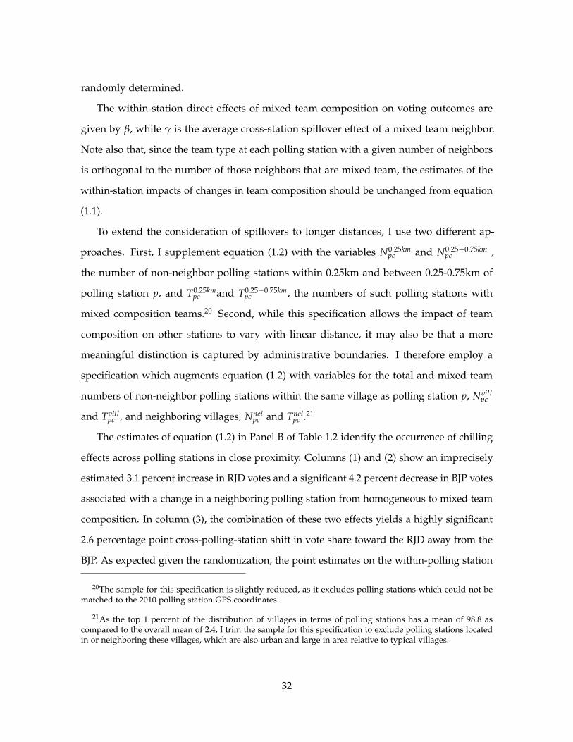
randomly determined.

The within-station direct effects of mixed team composition on voting outcomes are

given by β, while γ is the average cross-station spillover effect of a mixed team neighbor.

Note also that, since the team type at each polling station with a given number of neighbors

is orthogonal to the number of those neighbors that are mixed team, the estimates of the

within-station impacts of changes in team composition should be unchanged from equation

(1.1).

To extend the consideration of spillovers to longer distances, I use two different ap-

proaches. First, I supplement equation (1.2) with the variables N0.25kmpc and N0.25−0.75km

pc ,

the number of non-neighbor polling stations within 0.25km and between 0.25-0.75km of

polling station p, and T0.25kmpc and T0.25−0.75km

pc , the numbers of such polling stations with

mixed composition teams.20 Second, while this specification allows the impact of team

composition on other stations to vary with linear distance, it may also be that a more

meaningful distinction is captured by administrative boundaries. I therefore employ a

specification which augments equation (1.2) with variables for the total and mixed team

numbers of non-neighbor polling stations within the same village as polling station p, Nvillpc

and Tvillpc , and neighboring villages, Nnei

pc and Tneipc .21

The estimates of equation (1.2) in Panel B of Table 1.2 identify the occurrence of chilling

effects across polling stations in close proximity. Columns (1) and (2) show an imprecisely

estimated 3.1 percent increase in RJD votes and a significant 4.2 percent decrease in BJP votes

associated with a change in a neighboring polling station from homogeneous to mixed team

composition. In column (3), the combination of these two effects yields a highly significant

2.6 percentage point cross-polling-station shift in vote share toward the RJD away from the

BJP. As expected given the randomization, the point estimates on the within-polling station

20The sample for this specification is slightly reduced, as it excludes polling stations which could not bematched to the 2010 polling station GPS coordinates.

21As the top 1 percent of the distribution of villages in terms of polling stations has a mean of 98.8 ascompared to the overall mean of 2.4, I trim the sample for this specification to exclude polling stations locatedin or neighboring these villages, which are also urban and large in area relative to typical villages.

32

mixed team indicator are unchanged as compared to those from equation (1.1).

The results of tests for spillover effects over greater distances, defined in linear distance

and village boundaries, are shown in Panels A and B of Appendix Table A.5. While both

the within-station and cross-neighbor effects of team composition remain significant, the

estimates show no evidence of chilling or displacement effects over longer ranges.

1.6 Channel of impact: officer bias in discretionary decisions

Immediately prior to casting a vote at the polling station, each citizen must confirm her

identity as matching an individual on the list of registered voters at that station. The

verification process necessarily involves discretionary decisions by election officers, and so

is potentially susceptible to the influence of officer bias. In this section, I provide evidence

indicating that the process of voter identity verification is a major channel through which

team composition and officer bias interact to impact voting outcomes.

1.6.1 Vignette experiment: own-group bias in election officers

First, I test for election officer own-type bias in the evaluation of voting eligibility, using a

vignette experiment embedded within the survey of officers. I examine whether, holding all

other information constant, potential voters are more likely to be assessed by an election

officer as qualified to vote if they are of the same type as that official. Vignette experiments

have been used previously to address research questions in the electoral setting (Carlson 2010,

Banerjee et al. 2014) and are methodologically similar to the randomized CV experiment

approach that has been employed in the labor market discrimination literature (Bertrand

and Mullainathan 2003, Banerjee et al. 2009).

Each respondent was read a vignette describing a hypothetical individual attempting to

vote, with the wording identical across respondents with the exception of the individual’s

name, which was randomly assigned.22 Respondents were then asked to indicate the

22The vignette question was worded as: “Please consider the following situation: A voter named [RAN-DOMLY ASSIGNED] arrives at the polling station without an EPIC card but has a government voter’s slip

33

likelihood on a 4-point scale that the individual in the vignette would be able to cast a

vote. Each officer respondent was randomly assigned one of nine possible voter names.

Three names each were chosen to signal Muslim, Yadav, or Brahmin (the highest of Hindu

castes) identity in the hypothetical voter.23 To examine whether an officer’s evaluation of the

likelihood of a potential voter’s ability to cast a vote is influenced by whether that individual

is of the same type as the officer, I use regression specifications of the form:

Yqpc = µc + ϕn + πv + θMatchqpc + X′qpcλ + εqpc, (1.3)

where Yqpc is an outcome of officer q in polling station p in sub-constituency c, and µc

signifies sub-constituency fixed effects. Additionally included are fixed effects for the

randomly assigned potential voter name, ϕn, and election officer type, πv. Matchqpc is an

indicator variable taking value 1 if the election officer’s group type and that of the potential

voter are the same (e.g. Yadav and Yadav) and 0 otherwise. The potential-voter-name and

officer-type fixed effects control for the average differences in assessed likelihood of the

potential voter’s ability to vote across the different hypothetical names and by officers of

different types, so the coefficient of interest, θ, gives the average change in officer assessment

caused by the officer-voter type match. Further controls included are fixed effects for

polling team composition and a set of officer-level covariates: age, log monthly salary, an

indicator for first term of service at a polling station, and fixed effects for occupation type,

education level, and polling team position. A second specification additionally includes

polling-station-level controls for log total registered voters, share Muslim/Yadav registered

voters, and fixed effects for station location type and number of officer team members.

I consider as outcomes both an indicator variable taking value 1 if the officer indicates

the individual would be “Likely” or “Very Likely” allowed to vote and a continuous variable

taking the 1-to-4 scale value. Figure 1.5 shows that for both variables the average assessed

without a photograph. He can recite his name and other particulars. On a scale of 1 to 4, how likely do youthink it is that he would be allowed to cast a vote based on this information?", where the potential responses are“Very unlikely (1)”, “Unlikely (2)”, “Likely (3)”, “Very likely (4)”.

23Appendix Section A.2 provides the names used in each category.

34

Table 1.3: Vignette experiment: own-type bias in officer assessment of voters

Ability to cast vote0-1 indicator 4-point scale(1) (2) (3) (4)

Officer-potential voter name type match 0.103* 0.111** 0.237** 0.258**(0.056) (0.055) (0.117) (0.116)

Observations 871 869 871 869Name fixed effects X X X XOfficer type fixed effects X X X XIndividual controls X X X XPolling station controls X XNon-match group outcome mean [SD] 0.382 0.380 2.096 2.092

[0.486] [0.486] [0.974] [0.974]Notes: Columns (1) and (2) report OLS estimates from regressions at the officer level of an indicator variabletaking value 1 if the respondent answers "Very likely (4)" or "Likely (3)" as opposed to "Unlikely (2)" or "Veryunlikely (1)" to the question: "A voter named [RANDOMLY ASSIGNED] arrives at the polling station withoutan EPIC card but has a government voter’s slip without a photograph. He can recite his name and otherparticulars. On a scale of 1 to 4, how likely do you think it is that he would be allowed to cast a vote based onthis information?" and 0 otherwise, on an indicator variable for whether the officer’s own type matches that(Muslim, Yadav, Brahmin) of the randomly assigned voter name. Columns (3) and (4) report OLS estimates fromregressions with the 1-4 scale value as the outcome. Columns (1) and (3) include fixed effects for respondentname and officer type, the stratification variables (sub-constituency in which officer was assigned to a pollingstation and officer category [Muslim/Yadav at mixed polling station, non-Muslim/Yadav at mixed pollingstation, non-Muslim/Yadav at homogeneous polling station] plus the following individual level controls: age,log monthly salary, an indicator for first term of service at a polling station, and fixed effects for occupationtype, education level, and polling station position. Columns (2) and (4) further include polling station levelcontrols for log total registered voters and proportion Muslim/Yadav registered voters, and fixed effects forstation location type and number of team officers. Standard errors are clustered at the polling station level.*Significant at 10 percent. **Significant at 5 percent. ***Significant at 1 percent.

likelihood of voting increases significantly when the hypothetical individual is of the same

type as the election officer. Table 1.3 presents the underlying estimates from equation

(1.3). Considering the binary outcome variable, columns (1) and (2) show a significant 10

percentage point, or more than 25 percent, increase in the probability that an individual

is assessed as likely able to cast a vote. Similarly, using the 4-point-scale measure as the

outcome in columns (3) and (4), a significant increase of approximately 0.24 points is

observed.

35

0.1

5.3

.45

.6.7

50-

1 in

dica

tor

of v

otin

g ab

liity

like

lihoo

d

0 1Officer-voter name type match

11.

251.

51.

752

2.25

2.5

2.75

1-to

-4 s

cale

of v

otin

g ab

ility

like

lihoo

d

0 1Officer-voter name type match

Notes: The figure in the left panel depicts the estimated probabilities of an officer respondent indicating that ahypothetical individual described in the officer’s survey vignette would be “(3) Likely” or “(4) Very Likely” ableto cast a vote, as opposed to “(2) Unlikely” or “(1) Very Unlikely”. The estimates are based on the regression incolumn (2) of Table 1.3, assuming mean values of all control variables. The left bar represents the randomlyassigned subset of officer respondents for whom the hypothetical individual’s type (Muslim, Yadav, Brahmin)did not match the officer’s own type, while the right bar represents the subset for whom the types match. Thefigure in the right panel depicts the estimated 4-point scale values of a hypothetical individual’s voting abilitylikelihood, based on the same question as the left panel. The estimates are based on the regression in column(4) of Table 1.3, assuming mean values of all control variables. The notes to Table 1.3 provide the full vignettequestion text. Error bars signify 95 percent confidence intervals.

Figure 1.5: Own-type bias in officer assessment of voters

36

1.6.2 List experiment: biased officer behavior on election day

I next consider whether biased officer behavior was perceived as a relevant election day

phenomenon by voters and election officers in this setting. As direct elicitation of survey

respondents may yield unreliable estimates of the occurrence of potentially sensitive topics

such as biased officer behavior during elections, I employed list experiments in both the

surveys of registered voters and election officials. This method of indirect elicitation has

been used to generate measures of sensitive topics related to political and electoral behavior

in a number of recent papers (Gonzalo-Ocantos 2010, Corstange 2012, Kramon and Weghorst

2012, Ahlquist et al. 2013, Burzstyn et al. 2014).

For each list experiment, respondents were randomly assigned to either a control or

treatment group. Members of each group were asked to indicate only the total number

of statements that occurred at their polling station during the 2014 elections from a list

of statements read to them. Control respondents were given a list of four statements on

non-sensitive election day topics, while treatment respondents were read the same list

but with an additional sensitive statement included. This approach prevents individual-

level determination of which statements were chosen, but allows for the population-level

prevalence of the sensitive statement’s occurrence to be estimated as follows:

Nipc = αc + φTreatipc + X′ipcλ + εipc, (1.4)

where Nipc is the number of statements indicated as occurring at polling station p by

respondent i, Treatipc is an indicator variable for assignment to the group additionally

receiving the sensitive statement, and Xipc is a vector of polling station and individual

characteristics. Assuming that respondents assess the sensitive item truthfully and the

inclusion of the sensitive topic does not influence their evaluation of the non-sensitive items,

φ gives an unbiased estimate of the population proportion for whom the sensitive item

occurred. Standard errors are clustered at the polling station level. Additionally included

are polling-station-level controls for log registered voters, share Muslim/Yadav registered

voters and fixed effects for polling station number of officers and location type and for the

37

respective survey sampling strata. For officer-respondent regressions, individual controls

for age, log monthly salary and fixed effects for occupation type, education level, first term

of service, and team position are included. For voter-respondent regressions, controls for

age, gender, log monthly household income, and household head status and fixed effects

for occupation category and education level are included.

The survey of election officers included two list experiments.24 The sensitive statements

for the treatment group in the first and second experiments were: “One or more of the

election officers at the polling station treated some voters differently based on the voters’

religion or caste” and “One or more of the election officers tried to influence some voters’

choice of candidate or make it harder for them to vote”. Similarly, the two list experiments

included in the survey of registered voters had the sensitive statements: “One or more of

the election officers at your polling station treated you or others differently based on your

religion or caste” and “One or more of the election officers at your polling station tried

to influence how you or others voted or to make it more difficult for you or them to cast

votes”.

Table 1.4 presents the results of the list experiments. The estimates in column (3) of

Panel A indicate that 19 percent of officers agree that at least one of the officers at their

polling station treated voters differently based on religion or caste and 5 percent that at one

least member of their polling station team tried to influence voter behavior, whether choice

of candidate or making it more difficult to vote. I turn to the registered voter results in

Panel B. Estimates imply that 25 percent of respondents indicate that election officials at

their polling station treated voters differently based on religion or caste and 13 percent that

election officers tried to influence voting behavior at their polling station.

The wording of these statements is admittedly somewhat broad, and respondents

may vary in how they interpret them. Therefore, the aim of these experiments is not

to provide precise estimates, but rather to demonstrate the occurrence of biased officer

behavior connected to religion/caste on election day. The results, from both populations of

24Appendix Section A.2 provides the introductory prompt used in these experiments.

38

Table 1.4: List experiments: biased officer behavior on election day

Control Treatment Difference Obs.(1) (2) (3) (4)

Panel A. Election officers"One or more of the election officers at 1.915 2.086 0.192*** 878the polling station treated some voters [0.777] [0.873] (0.048)differently based on the voters’ religionor caste.”

"One or more of the election officers 2.883 2.960 0.047** 877tried to influence some voters’ choice [0.376] [0.398] (0.021)of candidate or make it harder for themto vote."

Panel B. Registered voters"One or more of the election officers at 2.036 2.280 0.254*** 3,532your polling station treated you or [0.758] [0.913] (0.026)others differently based on your religionor caste."

"One or more of the election officers at 2.396 2.539 0.128*** 3,547your polling station tried to influence [0.682] [0.809] (0.023)how you or others voted or to make itmore difficult for you or them to cast votes."

Notes: Columns (1) and (2) report unconditional means and standard deviations of the control (individualsreceiving a list of four questions with the listed statement omitted) and treatment (individuals receiving alist of the same four questions plus the listed statement included). Column (3) reports the coefficient of anOLS regression at the individual level of the total number of statements the respondent indicated occurredat the polling station during the 2014 elections and sub-constituency fixed effects. Additionally included arepolling-station-level controls for log total registered voters, share Muslim/Yadav registered voters, and fixedeffects for location type and number of officers. In Panel A, additional officer-level controls are age and logmonthly salary and fixed effects for occupation and education and controls for log monthly salary and priorelection experience. In Panel B, additional registered-voter-level controls are fixed effects for education leveland occupation type and controls for age, sex, household head status, and log monthly household income.Standard errors are clustered at the polling station level. *Significant at 10 percent. **Significant at 5 percent.***Significant at 1 percent.

39

respondents, suggest that officers do attempt to influence voting behavior on election day,

and that religion and caste influence their treatment of voters. In the sections which follow,

I conduct tests which allow for a further disentangling of mechanisms.

1.6.3 Election day experiences of potential voters

In this section I examine how the election day experiences of potential voters vary by officer

team composition, both in terms of overall station area management and the individual-

specific identity verification process. I use the following specification to test for impacts on

the frequency of canvassing or disorderly behavior at the polling station, as reported by

registered voter survey respondents:

Ywpc = µc + θo + βMixedpc + X′wpcλ + εwpc (1.5)

where Ywpc is an outcome for respondent w in polling station p in sub-constituency c. The

included individual and polling station controls are the same as in equation (1.4). In an

additional specification, I examine whether the reported impact of team composition differs

with respondent type by interacting the officer team composition variable with an indicator

for whether the respondent is Muslim or Yadav. Standard errors are clustered at the polling

station level.

Columns (1) and (3) of Table 1.5 show that the likelihoods of canvassing and disorderly

behavior are unaffected by team composition. Columns (2) and (4) further demonstrate that

the absence of significant differences holds regardless of respondent type. These results

suggest that stricter management of the area surrounding the polling station is not the

primary channel through which a shift from homogeneous to mixed team composition

impacts voting outcomes.

Turning to individual-specific experiences at the polling station, I employ the following

regression:

Ywpc = αpc + φMYwpc + λIDwpc + ψ(

MYwpc ∗ IDwpc)+ X′wpcλ + εwpc (1.6)

40

Table 1.5: Overall polling station management

DisorderlyCanvassing behavior

at station at station(1) (2) (3) (4)

Mixed team 0.005 0.002 -0.001 0.006(0.005) (0.007) (0.011) (0.014)

Muslim/Yadav -0.003 0.010(0.006) (0.014)

Muslim/Yadav * Mixed team 0.006 -0.018(0.010) (0.019)

Observations 3,733 3,733 3,775 3,775Polling stations 351 351 351 351Outcome mean [SD] 0.020 0.020 0.068 0.068

[0.141] [0.141] [0.256] [0.256]Notes: All columns report OLS estimates from regressions at the individual level of the listed variable onan indicator for mixed officer team composition at the polling station. Even-numbered columns include aninteraction with an indicator for whether the respondent is Muslim/Yadav. Additionally included in all columnsare fixed effects for the stratification variables (sub-constituency and above-below district level median in termsof MY elector percentage) and individual-level controls for age, sex, education level, household head status,household structure type, occupation type, and log monthly household income. Polling-station-level controls areincluded for log total registered voters, share Muslim/Yadav registered voters, and fixed effects for the numberof officers stationed at the polling station. Standard errors clustered at the polling station level. *Significant at10 percent. **Significant at 5 percent. ***Significant at 1 percent.

41

where αpc are polling station fixed effects and IDwpc is an indicator for voter identity card

possession by individual w at polling station p. I estimate this regression separately for

individuals in the randomly determined samples of mixed team and homogeneous team

polling stations. The same set of registered-voter-level controls from equation (1.4) are

included and standard errors are clustered at the polling station level.

I first consider a potential voter’s ability to cast a vote as an outcome. I find in column

(1) of Table 1.6 that, at polling stations with homogeneous officer teams, individuals

are significantly less likely to be able to vote if they are Muslim/Yadav. This difference

disappears among individuals with voter identity cards, which reduce the scope for officer

discretion. In addition, for non-Muslim-Yadav individuals, possession of a voter identity

card does not significantly change the likelihood of being able to cast a vote. Column (2)

shows that, at polling stations with mixed officer teams, voter identity card possession

significantly increases the likelihood of being allowed to cast a vote, but that this no longer

varies with Muslim/Yadav identity. These regressions include a variety of individual-level

controls, reducing concerns that the effects are driven by correlations between Muslim/Yadav

identity or voter identity card posession with unobservables that influence voting ability. To

summarize, at homogeneous team stations, voter identity cards matter in terms of voting

ability only for Muslim/Yadav potential voters, while at mixed team stations they are

important for potential voters of all types.

I subsequently examine as an outcome the likelihood of a potential voter having a

satisfactory overall experience at the polling station on election day.25 Column (3) shows

that Muslim/Yadav potential voters facing homogeneous teams of officers rate their polling

station experiences as worse on average, but only in the absence of voter identity cards. Non-

Muslim/Yadav voters, however, express lower satisfaction if they possess a voter identity

card. The latter effect could reflect that under-qualified non-Muslim/Yadav potential voters

are relatively more appreciative of being allowed to vote than those with voter identity

25This variable takes value 1 if a respondent indicates that her overall voting experience at the polling stationon election day was “Excellent”,”Good”, or ”Fair”, as opposed to “Poor”.

42

Table 1.6: Identity verification experience of potential voters

Satisfactory overallAble to cast vote station experienceHomog. Mixed Homog. Mixed

team team team team(1) (2) (3) (4)

Muslim/Yadav -0.104* -0.047 -0.066+ 0.001(0.062) (0.066) (0.041) (0.031)

Possess voter identity card 0.011 0.105** -0.019* 0.013(0.025) (0.046) (0.010) (0.024)

Muslim/Yadav * Possess voter identity card 0.109* 0.033 0.072* -0.004(0.062) (0.066) (0.043) (0.033)

Observations 1,929 1,946 1,907 1,900Polling stations 175 176 175 176Outcome mean [SD] 0.981 0.980 0.981 0.982

[0.137] [0.138] [0.136] [0.133]Notes: All columns report OLS estimates from regressions at the individual level of the listed variable on aninteraction of the Muslim-Yadav respondent indicator with an indicator for voter identity card possession,for the sample of polling stations indicated in each column. Additionally included are polling station-levelfixed effects and individual-level controls for age, gender, education level, household head status, householdstructure type, occupation type, and log monthly household income. “Satisfactory overall station experience” isan indicator for whether the respondent indicated that their overall voting experience at the polling station onelection day was “Excellent”/”Good”/”Fair”, as opposed to “Poor”. Standard errors clustered at the pollingstation level. *Significant at 10 percent. **Significant at 5 percent. ***Significant at 1 percent. + p-value = 0.112.

43

cards, who are more certain that they should be allowed to do so. I find in column (4) that

these impacts are absent at mixed team polling stations. Overall, the results in Table 1.6 are

consistent with mixed team composition and voter identity card provision each reducing

the differential treatment of potential voters at polling stations, where homogeneous teams

are relatively more stringent toward Muslim/Yadavs.

1.6.4 Heterogeneity in effects by voter identity card coverage

Using experimental and survey data, the previous sections established that election officers

are relatively biased in favor of potential voters of their own type and that individuals’

religious and caste identities can influence their ability to vote if they do not have a

voter identity card. If in general identity card possession reduces the scope of potentially

discriminatory discretion available to officers and mixed team composition shifts station

administration of the voter identification process to be more neutral, a substitute relationship

in the impacts of the two on polling-station-level voting outcomes would also be expected.

Returning to the polling station administrative data on voting outcomes, I test for this

substitutability using specifications of the form:

Ypc = µc + θo + βMixedpc + η(Mixedpc ∗ IDc) + X′pcλ + εpc, (1.7)

where IDc is the proportion of registered voters in sub-constituency c without a voter identity

card.26 Polling-station-level controls included are the log number of registered voters and

the Muslim/Yadav share of registered voters. The top one percent of observations in terms

of the absolute value of the vote share margin between the RJD and BJP are trimmed.27

The main effect for IDc is absorbed by the sub-constituency-level fixed effects, and the

coefficient of interest is η, where an estimated sign opposite that of β indicates that polling

station composition and voter identity card coverage exhibit substitutability in their impacts

on voting outcomes. Sub-constituency-level voter identity card coverage is not randomly

26The lowest level at which data on voter identity card coverage is available from the government.

27These are polling stations where one coalition won by a margin of at least 88 percent.

44

Table 1.7: Heterogeneity in effects of team composition by voter identity card coverage

Vote shareLn votes RJD Ln votes BJP margin RJD-BJP(1) (2) (3) (4) (5) (6)

Mixed team * -0.009* -0.014* 0.005 0.010* -0.004** -0.006**Voter identity card coverage % (0.005) (0.008) (0.004) (0.006) (0.002) (0.003)

Mixed team 0.809 1.072 -0.453 -0.960* 0.383** 0.558*(0.457) (0.768) (0.332) (0.579) (0.173) (0.314)

Observations 5,429 5,429 5,439 5,439 5,442 5,442Polling station controls X X X X X XSub-constituency fixed effects X X X X X XInteracted sub-constituency controls X X XImplied effect: minimum sample 0.129** 0.152*** -0.079** -0.086** 0.063*** 0.072***card coverage sub-constituency (0.054) (0.057) (0.040) (0.043) (0.022) (0.024)

Notes: All columns report OLS estimates from regressions at the polling station level of the listed variable on anindicator for mixed team composition interacted with the sub-constituency-level percentage of registered voterswith a voter ID card. Also included are sub-constituency and number of officer fixed effects and controls forMuslim/Yadav share of registered voters and log total registered voters. Even-numbered columns additionallyinclude interactions (not shown) with sub-constituency-level measures of the population proportions that areliterate and Schedule Caste/Schedule Tribe, and the share of registered voters that are Muslim/Yadav (noneof these interaction effects are statistically significant). The implied effect given in each column reflects theestimated impact of mixed team composition for the sub-constituency with the lowest level of voter identity cardcoverage observed in the sample. Coverage ranges between 76.3 and 93.9 percent in sample sub-constituencies.The sample trims the top one percent of observations in terms of absolute value of coalition vote share margin(polling stations with a margin greater than 88 percentage points). *Significant at 10 percent. **Significant at 5percent. ***Significant at 1 percent.

determined, and may be correlated with other characteristics that mediate the impact of team

composition on voting outcomes. As a robustness check I therefore consider a specification

where I additionally interact officer team composition with sub-constituency-level measures

of the population proportions that are literate, Scheduled Caste/Scheduled Tribe, and

Muslim/Yadav.

In columns (1) and (2) of Table 1.7, I find that the positive impact of mixed team

composition on RJD votes decreases by a significant 0.9 percentage points per 1 percentage

point increase in voter identity card possession. The results for BJP votes in columns (3)

and (4) also indicate that the team composition effects are strongest in areas with low voter

identity coverage. Columns (5) and (6) show that the vote share margin shift toward the RJD

caused by changing from a homogeneous to a mixed team is approximately 0.5 percentage

points smaller per 1 percentage point increase in voter identity card coverage.

45

-.15

-.05

.05

.15

.25

Impa

ct o

f mix

ed te

am c

ompo

sitio

non

RJD

-BJP

vot

e sh

are

mar

gin

.7 .8 .9 1Sub-constituency-level voter identity card coverage

Notes: Figure plots the estimated polling-station-level impact of mixed team composition on the vote sharemargin between the RJD and BJP coalitions at different levels of sub-constituency-level voter identity cardcoverage. Dashed lines signify 95 percent confidence intervals. Calculated using the estimates from Column (5)of Table 1.7.

Figure 1.6: Heterogeneity by voter identity card coverage in impact of team composition

Voter identity card coverage in my sample of sub-constituencies ranges from 76.3 to

93.9 percent. Figure 1.6 plots the implied effect of mixed team composition over a similar

range of voter identity coverage and demonstrates that the significant impact observed at

low coverage levels becomes insignificant as full coverage is approached. These estimates,

taken together with the earlier experimental and survey results, provide strong evidence

that mixed team composition and identity card coverage serve substitute roles in preventing

officer bias from undermining the neutrality of the identity verification process for potential

voters.

46

1.7 Alternative explanations

A possible concern in attributing the previously identified impacts to bias associated with

officers’ religious and caste identities is that there may exist other characteristics that

correlate with these identities and also influence voting outcomes. This is unlikely to explain

the above results for two reasons: the previous analysis captures the effects of the presence

on otherwise homogeneous teams of officers that are either Muslim or Yadav, two groups

which are not particularly similar outside of their political alliance; and indviduals of

different religions and castes serving as polling station officers are more likely to be similar

along other dimensions than would be their populations in general.

First, Yadavs are a lower-caste Hindu group in Bihar and, other than in political orien-

tation, it is unclear along what dimensions they would be systematically more similar to

Muslims than to other Hindu groups, especially given the dispersed support for the BJP

across upper- and lower-castes in these elections.28 In Appendix Table A.6, I examine the

influence of Muslim and Yadav officer presence separately using a regression specification

analogous to that of equation (1.1). The estimates across columns (1) through (4) reveal

similar impacts for Muslim and Yadav officers. The coefficients for the two groups are

statistically indistinguishable in each case, and the shift in vote share margin toward the RJD

is significant at the 5 percent level for both Muslim and Yadav presence on officer teams.

Second, polling station officers are selected from pools of government employees who

are likely more similar than would be average individuals from different religious and

caste groups. I explicitly test for differences by Muslim/Yadav status in the sample of

surveyed polling station officers across a number of characteristics proxying for experience

and knowledge: age, log monthly salary, college graduation, and prior election officer

experience. I regress each of these outcomes on an indicator variable for Muslim/Yadav

identity and fixed effects for sub-constituency and team position. As a further check, I also

28Highlighting the differences between the two groups, Lalu Prasad Yadav, the politician responsible for thecreation of the Muslim/Yadav coalition, has even said “I have made an alliance between those who worship thecow [Yadavs] and those who eat the cow [Muslims].” (Wittsoe 2013, p.60)

47

Table 1.8: Variation in other officer characteristics by Muslim/Yadav identity

Survey data Administrative dataLn First Ln

monthly College time monthlyAge salary graduate officer Age salary(1) (2) (3) (4) (5) (6)

Muslim/Yadav officer -0.340 0.018 -0.025 -0.019 0.439 0.001(0.554) (0.029) (0.030) (0.031) (0.373) (0.012)

Observations 912 888 911 903 5,983 6,198Non-Muslim/Yadav 42.822 9.563 0.684 0.333 44.975 9.291outcome mean [SD] [9.727] [0.584] [0.465] [0.472] [9.802] [0.363]

Notes: All columns report OLS estimates from regressions at the officer level of the listed variable on anindicator for Muslim/Yadav identity. Additionally included are sub-constituency and officer-position fixedeffects. Columns (1) through (4) are based on reported data from the survey of officers. Columns (5) and (6) arebased on full sample of administrative data available for the same district in which the surveys were conducted.*Significant at 10 percent. **Significant at 5 percent. ***Significant at 1 percent.

construct measures of age and log monthly salary based on separate administrative data

available for the full population of election officers in the district in which the officer survey

was conducted. The results in columns (1) through (6) of Table 1.8 show that in no case are

there significant differences by Muslim/Yadav status.

1.8 Conclusion

Having identified significant impacts of officer team composition on voting outcomes

within and across polling stations, a natural question is whether changes in composition

influence who ultimately wins elections. To examine this possibility, I conduct counterfactual

calculations of the effects of alternative officer assignment mechanisms on the identities of

winners in the 2014 parliamentary elections in Bihar.

I first use administrative data available across the state of Bihar to calculate the sub-

constituency-level average numbers of neighbor polling stations. Second, the observed

margins of victory from these elections already reflect the effects of the underlying (but

unobserved outside of the two study districts) proportions of mixed team polling stations

48

in each parliamentary constituency. Finally, I assume that the proportion of mixed team

polling stations in each sub-constituency is the same as the average value (0.324) across

the two districts for which it can be directly observed in my data. I can then calculate

the magnitudes of the shifts in the proportions of homogeneous and mixed team polling

stations required to change the outcome of each election in which the RJD and BJP coalitions

were both either winner or runner up.29

I use these magnitudes to consider the effects of two alternatives to the current method of

randomized officer assignment: (1) requiring mixed team composition in all polling officer

teams, and (2) excluding Muslim/Yadav officers from teams. During the 2014 elections, the

RJD and BJP fielded the top two candidates in 29 of the 40 parliamentary constituencies

in Bihar (Appendix Figure A.4 provides the distribution of vote share margins). As shown

in Table 1.9, a shift to Alternative 1 is estimated to switch one election outcome in favor

of the RJD and a shift to Alternative 2 to change one outcome to a BJP victory. I repeat

this exercise for the most recent prior state assembly elections in 2010, where the RJD and

BJP fielded the top two candidates in 185 of 243 races. Reflecting the lower levels of voter

identity card coverage and greater number of close contests, thirty-three races are estimated

to change to an RJD victory under Alternative 1 and six elections to switch in favor of the

BJP under Alternative 2, or a combined 16 percent of the total.

In addition, the religious composition of candidates put forward in elections differs

considerably across the coalitions; 17.5 percent of RJD coalition candidates in the 2014 Bihar

elections were Muslim, as compared to just 2.5 percent for the BJP coalition. Accounting for

the religious identities of candidates, the previous counterfactual calculations also indicate

that a shift to all mixed team polling stations in Bihar would have led to a 25 percent

increase in Muslim legislators both in the 2010 assembly and 2014 parliamentary elections.

Recent work has shown that increasing Muslim representation in state legislatures in India

results in significant reductions in child mortality rates and gains in educational attainment

29Appendix Section A.3 additional details. The vote share margin between the runner-up candidate and theremainder of the field is generally large enough that having a third place or lower candidate shift to become thewinner could not feasibly occur as a result of changes in team composition.

49

Table 1.9: Changes in election outcomes under alternative officer assignment mechanisms

Alternative 1: Alternative 2:All mixed teams No mixed teams

Vote Vote RJD/BJP to share RJD to share BJPRJD margin BJP margin top two Total

victory range victory range parties races(1) (2) (3) (4) (5) (6)

National parliament, 2014 1 -0.024 1 0.010 29 40

State assembly elections, 2010 33 [-0.066, 6 [0.004, 185 243-0.0003] 0.023]

Notes: This table reports estimates of the potential number of races for which the winning candidate would haveswitched between the RJD coalition and the BJP coalition, under two alternative officer assignment scenarios.Alternative 1 is the presence of all mixed composition teams and Alternative 2 is the absence of any mixedcomposition officer teams, assuming an initial 0.324 proportion of mixed teams (that observed in the available2014 data). Columns (1) and (3) give the number of races for which the winning party would change asindicated. Columns (2) and (4) give the range of the RJD-BJP coalition vote share margins observed in theimpacted constituencies. Column (5) gives the number of races in which the RJD and BJP coalitions fielded thetop two candidates, and column (6) the total number of races in Bihar for that election cycle. The calculationaccounts for spillover effects from neighboring mixed team polling stations and heterogeneity in impact byvoter identity card coverage (at the sub-constituency level).

across both Muslim and non-Muslim households (Bhalotra et al. 2014). This suggests that

the impacts on election outcomes associated with officer team composition may also have

important downstream effects on outcomes directly relevant to citizen well-being.30

Fair and well-functioning elections are critical to maintaining the responsiveness of

elected officials to citizens in democracies. While the related literature on election reforms

has focused in large part on the benefits of advances in monitoring and voting technology,

this paper is to my knowledge the first to provide rigorous evidence of the remaining impor-

tance of the identities of local-level election personnel. Indian elections are technologically

advanced and their administration is highly regulated, indicating that bias in discretionary

decision making of polling station officers can undermine the quality of service provision

30It is also possible that the effects of officer team composition on citizens’ election day experiences influencetheir expectations and behavior in subsequent elections, for instance in whether to turn out at the polling station.I use polling-station-level data for the 2015 state assembly elections in Bihar and find in Appendix Table A.7that voting outcomes in these elections are unaffected by officer team composition from 2014, providing noevidence of cross-election-cycle impacts on voter behavior.

50

even at the present frontier of election practice.

Though my findings suggest that diversity within teams of election officers can im-

prove the impartiality of polling station management, it may not always be politically or

administratively feasible to mandate that such mixed composition occur. It could also be

difficult in other contexts to determine the relevant dimensions of identity along which

diversity should be defined. My results, however, additionally demonstrate that policies

which reduce the scope for officer discretion in the first place, such as the widespread

provision of voter identity cards, may be promising alternatives in reducing the ability of

local-level election officials to influence voting outcomes. More generally, the findings of this

paper demonstrate that institutions which require greater discretionary decision making by

bureaucrats or other government employees may be more susceptible to adverse impacts of

these individuals’ underlying biases on the quality of public services.

51

Chapter 2

Can Electronic Procurement Improve

Infrastructure Provision? Evidence

from Public Works in India and

Indonesia1

2.1 Introduction

Contestable government procurement of goods and services has been estimated at over 7

percent of world GDP (OECD 2002), with the incidence rising in emerging economies: For

instance, in 2007, the Indian government spent over US $21 billion ($18 per capita) on the

procurement of external goods and services, over double what it spent in 2000 (IMF). Yet,

both the quantity and quality of recently constructed public infrastructure often remain

low (Briceño-Garmendia, Estache, and Shafik 2004). A limited supply of local qualified

contractors, collusion among contractors, and corruption among public officials have each

been cited as important reasons (Kenny 2007).

1Co-authored with Sean Lewis-Faupel, Benjamin A. Olken, and Rohini Pande

52

A number of governments have responded by adopting electronic procurement (hence-

forth: e-procurement) (World Bank 2007). Broadly, e-procurement is the implementation

of a technological platform as directed by a potential buyer (a government agency or firm)

to facilitate transactions between that buyer and potential sellers of goods and services.

Commonly, the practice includes electronic postings by the buyer of products and services

desired for procurement. There is often an online method for potential suppliers to offer

those goods or services requested by the buyer, under a contract and price either preor-

dained by the buyer or offered by the potential seller. As with traditional procurement, there

is typically a method for choosing among contracts or prices offered by the potential sellers.

In some cases, this selection process is performed automatically by the technology.2 In other

cases, e-procurement consists of contracted sellers providing a set of goods or services at

fixed prices from which the buyer can choose as needed. Additionally, e-procurement may

allow for the electronic transfer of funds as agreed upon in the procurement contract. Finally,

the technology can facilitate a review by the buyer of the goods or services delivered by

the contracted seller, which may be communicated to the seller, considered when enforcing

contracts, and used by the buyer in future procurement decisions. We describe the specifics

of the e-procurement reforms in the Indian and Indonesian contexts in the next section.

E-procurement can potentially address three common concerns with manual procure-

ment practices: lack of access to bid information, collusion among bidders, and corruption.

By lowering the costs of obtaining information about a tender process, e-procurement may

increase the number of firms who can bid. Likewise, it can reduce bidder collusion by

providing tender information to firms outside a local cartel, allowing non-cartel firms to

participate and breaking up local bidding cartels. E-procurement can also mitigate cor-

ruption by reducing government officials’ ability to selectively withhold information or

refuse electronic bids from non-favored bidders. Moreover, by ensuring public access to

2The system may also allow potential sellers to electronically submit other supporting documentation, suchas resumes or technical capabilities, or allow the buyer and potential sellers to communicate electronically.Additionally, e-procurement may be used to record and archive any number of other data points of interest tothe buyer.

53

all procurement data, e-procurement enhances transparency and the possibility of public

oversight.

However, it is plausible that in low income settings, where information technology

coverage and other aspects of state capacity remain low, e-procurement can only effect

limited change and can potentially make things worse. Potential contractors (who are

currently not in the system) may continue never to learn about available tenders, and

cartels and corrupt officials may continue to use strong-arm tactics to prevent entry by such

contractors. If many small firms have limited access to the internet, requiring electronic bids

could harm competition.

In this paper we examine the impact of electronic procurement on public works projects

in two large emerging economies: India and Indonesia. In India, we examine procurement

practices between 2000 and 2009 for a federally funded rural road construction program

which is implemented by state road departments, the Pradhan Mantri Gram Sarak Yojana

(PMGSY) program. Under this program, roughly 145 road packages were tendered per

state per year. In Indonesia, we examine contract data from the national Ministry of Public

Works for both construction and consulting (e.g., engineering management and design)

contracts each year. On average, 32 consultancy and 58 construction packages per province

were issued each year. The gradual roll-out of e-procurement (at the state-level in India

and province-level in Indonesia) allows for a difference-in-differences strategy: We compare

outcomes in states/provinces before and after the adoption of e-procurement, as well as in

those continuing under manual procurement practices, allowing us to quantify the benefits

or costs of the practice in both countries.

For both countries, we obtained administrative data on the complete universe of contracts

from before and after e-procurement by scraping publicly available information from

respective government websites. In Indonesia we have bidding and final contract data for all

tenders; in India, the website publishes final contract data but not the details on individual

bids. All told, this leaves us with a dataset of over 20,000 contracts in India and over 14,000

tenders in Indonesia. In addition, in India, we hand collected bidding data on tenders for

54

four states which we use to supplement the administrative data.

We first show that, in both India and Indonesia, e-procurement increases the probability

that the winning bidder comes from outside the region where the contract takes place.

This is consistent with e-procurement decreasing the costs of submitting bids for those

not physically present. We next examine the impact on the ultimate outcomes of interest:

price, quality of construction, and timeliness. We find no systematic evidence that electronic

procurement lowers prices paid by the government. In Indonesia, the point estimates

are consistent with small (2-5 percent) reductions in prices, but these are not statistically

significant. In India, final prices are unaffected. Overall, we can statistically rule out (at the

5 percent level) declines in contract values of more than 2.7 percent in India, of more than

6.6 percent for Indonesian consulting projects, and of more than 14.1 percent for Indonesian

works contracts.

In contrast, e-procurement led to quality improvements, albeit along different dimensions

in the two countries. A first measure of quality is time-overrun in project completion. Reports

of corruption of procurement in India typically focus on cases where works are abandoned

halfway through or completed in a very tardy manner. In our data we see that 77 percent

of road projects in India and around 95 percent of public works projects in Indonesia

are completed late. In India, we observe no statistically significant changes in late works,

while in Indonesia these declines are large and significant – whereas only 5 percent of

conventionally procured construction projects in Indonesia are completed on schedule, 20

percent of electronically procured construction projects are on time.

A separate indicator of quality, only available for India, is an independent audit report

on construction quality, which was conducted identically in roads completed under both

e-procurement and traditional procurement. According to this measure, we find that e-

procurement leads to higher quality roads, with the quality grades rising by about 12 percent

in e-procurement projects compared to other projects.

We then explore the degree to which the results are driven by improving outcomes

among already winning bidders, as opposed to changing who wins. To see whether the

55

observed changes in outcomes reflect changes in selection of who wins, for the key variables

of interest – price, delays, and quality – we estimate a fixed effect for each contractor

and examine how e-procurement changes the average quality characteristics of winning

contractors (i.e., the fixed effects of who wins). We find that after e-procurement, winning

contractors in India tend to be those who have higher quality on average. In Indonesia,

we find evidence that those contractors who win after e-procurement are systematically

less likely to be late. This suggests that a key mechanism for e-procurement is allowing

higher quality contractors to enter and win projects, rather than simply encouraging better

performance from an existing set of contractors. Increased entry of contractors could reflect

better information flows and/or reduced ability of local contractors to prevent others from

filing tenders.

This paper is related to several economic literatures. While there is a growing body of

work which examines procurement (Bandiera, Prat, and Valletti 2009, Krasnokutsaya and

Seim 2011), much of the literature has focused on the award procedures (i.e., scoring auctions

vs. lowest-price auctions, etc.) (Tran 2008) and potential interactions with other procurement

regulations (Decarolis 2014). This paper suggests that an important component, at least for

ensuring quality, can be in the implementation of the procurement auction, holding these

rules fixed. It also contributes to a growing literature using procurement data to examine

corruption (Di Tella and Shargrodsky 2003, Ferraz and Finan 2008, Bandeira, Prat, and

Villetti 2009, Bobonis, Fuertes, and Schwabe 2010, Cai, Henderson, and Zhang 2013).

Second, past work has highlighted the role of media and technology in shaping the

political and policy landscape. Strömberg (2004) suggests that media access among con-

stituents may make politicians more responsive to voters, while Falck, Gold, and Heblich

(2012), Jaber (2013) and Campante, Durante, and Sobbrio (2014) measure causal impacts of

internet access on political participation. Our paper complements this previous literature

by considering how new technology, in this case implemented by government itself, may

improve the outcomes of a government initiative.

Finally, this paper is part of a recent, broader agenda that documents the role of

56

communication technology in development. While there are several studies that document

the impact of cell phone technology on market access (Jensen 2007, Aker 2010) and education

(Aker, Ksoll, and Lybbert 2012), this paper represents one of the first studies to examine the

impact of the internet on governance issues.

One advantage of our approach is that we use the same methodology to study separate

e-procurement programs in two different countries. To the extent that the findings from

both countries are similar, the external validity of our results is given credence. To the best

of our knowledge, this study represents one of the first microeconomic studies that uses

difference-in-differences to simultaneously evaluate a new program in multiple countries,

allowing for more careful conclusions with respect to external validity.3

The paper is structured as follows: In Section 2.2 we describe the institutional details

relating to procurement practices and road construction in India and Indonesia. In Section

2.3 we describe the data and empirical strategy. In Section 2.4 we report the findings. Section

2.5 concludes.

2.2 Background

We start by describing the public works programs in our two study countries, followed by

the nature of e-procurement adopted in these two settings. We conclude the section with a

brief description of likely channels of influence of e-procurement.

2.2.1 India

Public Works Program and Manual Procurement

In the year 2000, India launched a large-scale rural road construction scheme called Pradhan

Mantri Gram Sarak Yojana (PMGSY). The federal government provides funding for this

scheme and coordinates program implementation, but full executional responsibility lies

3The other study of this nature we are aware of is Gruber and Mullainathan (2005), which evaluates theimpact of state and provincial cigarette tax changes in the US and Canada.

57

with state governments. Each state has a rural roads department which decides the schedule

for road construction and manages procurement. PMGSY roads follow a uniform criteria

for road construction in terms of material usage and quality for all Indian states.

For PMGSY, all states use the same procurement rules and standardized bidding docu-

ment, provided by the national roads agency. The procurement process follows a cost-based

auction procedure. Specifically, conditional on meeting a pre-specified set of technical

qualifications intended to ensure a contractor is capable of completing the project, the

contract is awarded to the lowest bidder. Importantly, these rules are identical for manual

and electronic procurement.

Anecdotally, public procurement in India is rife with corruption, and claims of impropri-

ety exist throughout the contracting process. Contractors have reported being physically

intimidated or barred from submitting bidding documents. The handling of bidding doc-

uments after submission has also been called into question with claims of altered bids,

inspection of bids prior to technical reviews, and intentional loss of submissions. There is

also concern that technical qualifications are used to unreasonably exclude certain firms

from the bidding process. The implication of many of these reports is that government

officials collect rents in exchange for some advantage in the bidding process.

As a case study, we examined the tendering process for manual procurement for a

random sample of 188 road contracts issued between 2001 and 2005 in the Indian state of

Uttar Pradesh. As Figure 2.1 shows, there is very little competition in PMGSY contracts. In

95 percent of cases, the price bid of only one firm was evaluated; that is, there was only one

bid submitted or all other bids were disqualified based on technical requirements. When we

observe multiple bids here, over three quarters of the time all but one bid are disqualified.

In the case of any technical disqualification, all but one bidder are disqualified 100 percent

of the time. Prima facie this pattern of disqualifications is consistent with corrupt officials

enforcing a desired winner.

In 2000, when the program began, all Indian states used a manual paper-based procure-

ment system to bid out contracts to private contractors. This process involved obtaining

58

Number ofNumber technicalof disqualificationsbidders 0 1 2 3 41 1552 5 143 1 54 3 45 1Total 164 14 5 4 1

Notes: Figure presents bidding data from a random sample of 188 road contracts issued between 2001 and2005 in the Indian state of Uttar Pradesh (prior to e-procurement). Each cell is a count of tenders with therespective number of bidders and technical disqualifications. Technical disqualifications are intended to preventa bidder who lacks the necessary expertise or equipment from competing. Blank cells indicate zeros. Note thatthe diagonal comprises all cases of all-but-one disqualified.

Figure 2.1: Number of contracts by numbers of technical disqualifications and bidders

internal approval of the project, publishing a Notice Inviting Tenders (NIT) in several media

outlets (typically newspapers), having suppliers obtain detailed bid preparation materials

from the government, receiving bid submissions from suppliers, receiving bid evaluations

by buyers, and finally, the awarding of the procurement order and signing of agreements.

The complete process required a long chain of internal authorizations (at times involving

several departments), several visits by suppliers to departments, and the generation of reams

of paper-based statements and evaluations.

E-Procurement

The Indian IT Act of 2000 provided legal recognition to electronic transactions. Since

then, several Indian states have passed legislation enacting e-procurement, and the rural

roads department in several states followed by adopting e-procurement practices for road

construction. The implementation of e-procurement for PMGSY typically involves placing

all invitations for tender into an online, searchable database. An online portal is also

established that allows authorized users (contractors) to upload bidding materials. The

Indian e-procurement systems prohibit procurement officials from viewing contractor names

and viewing or editing price bids before completing the technical certification process, in

59

Figure 2.2: E-procurement adoption - India

theory preventing favoritism in the selection process. Given the above description of how

most bidders are disqualified during the technical stage, this is potentially important for

preventing corrupt practices. Finally, much of the electronic data is stored after auctions are

completed, creating the potential for accountability.

We exploit this variation across time and states for our empirical analysis. Our sample

covers 27 Indian states and territories during the period January 2000 through August 2009.

During this time frame, 9 states adopted a system of electronic procurement. Figure 2.2

shows the dates when e-procurement rules were adopted in various states through August

2009. The first state to adopt, in 2004, was Andhra Pradesh, which (along with Karnataka)

is one of the technological leaders of India. (Note that in some states (Chattisgarh, Gujarat,

and Orissa), contracts which are below a state-specified cost threshold do not go through

the electronic procurement process and are processed on paper. Since the threshold may

respond endogenously to the auction policy (see, e.g., Tran 2008), during the applicable

periods, we classify all projects as electronically tendered in these states.)

60

2.2.2 Indonesia

Public Works Program and Manual Procurement

In Indonesia, we examine the national Ministry of Public Works (MPW). The MPW procure-

ment process covers mainly two types of contracts, works and consulting. Works contracts

refer to projects such as the building or repairing of roads and bridges, where physical ser-

vices or construction work are conducted by the contract winner. Access to heavy equipment

and various construction materials is therefore typically a necessary component for these

projects. Consulting contracts, in contrast, entail the provision of professional expertise by

the winning bidder in planning or supervision services such as design and management.

Depending on the project, procurement takes place either at the national headquarters in

Jakarta or at the provincial offices of the MPW.

Works and consulting contracts additionally differ in the structure of their bidding

processes. Works contracts are generally assigned to the low bidder conditional on meeting

minimum administrative and technical qualifications, as in India. Consulting contracts

involve a pre-qualification phase in which potential bidders first submit a document con-

taining administrative, financial, and work experience information. A shortlist of firms

meeting minimum qualification requirements are then invited to submit technical and cost

bids. The winning bidder is assigned using a formula based on a combination of technical

score and price, rather than simply lowest bid conditional on meeting minimum technical

requirements as with works projects. For both types of contracts, a minimum of three bid

submissions are required; otherwise, the processes are repeated. The overall pool of bidding

firms consists of both private firms and state-owned construction firms, with state-owned

firms competing against the private sector without any special preferences.

Public procurement is widely considered “one of the most corruption-ridden sectors”

(Freedom House 2012) in Indonesia. For example, the 2009 Enterprise Survey of Indonesia

(World Bank and IFC) sampled 1,444 firms comprising a representative sample of the non-

agricultural formal private economy in the country. In the survey, 38.1 percent of respondents

who had attempted to secure a government contract in the previous year indicated that firms

61

with characteristics similar to theirs make informal payments or give gifts to public officials

to secure such contracts, though the average value given for these bribes was only 1.8

percent of the total contract value. A separate survey of 792 randomly sampled construction,

consulting, and supplier firms conducted in 2010 by the Indonesia Procurement Watch

(Indonesia Procurement Watch 2011) provides further suggestive evidence of corruption in

the government procurement process, with 92.7 percent of respondents answering that they

thought their firm had ever given bribes to the government officials involved in managing

procurement. Additionally, 97.3 percent of respondents believed that it was not possible

to win the contract tender without bribery and more than 95 percent indicated that the

typical value of a bribe was more than 10 percent of the contract value. Beyond survey

results, of the 196 cases considered by the Corruption Eradication Commission (KPK) of the

Government of Indonesia between 2004 and 2010, 86 dealt with bribery and graft related to

the procurement of goods and services and every such case resulted in a conviction (Onishi

2009, Parlina 2011).

Anecdotal evidence suggests that the manual procurement process contributes to the

corruption problem in much the same ways as discussed in India. For example, government

officials may not make the detailed documents required to prepare a bid available to non-

favored firms or purposely misinform them about the proper submission process (UNAFEI

2008). Alternatively, there could be physical intimidation of firms that are not part of the

cartel from submitting bids.

E-Procurement

Indonesia began rolling out a “semi-electronic procurement” (SEP) system in 2004 in the

central ministry in Jakarta and expanded the procedure across the 33 provincial offices in

approximately concentric circles from Jakarta over the next 5 years, as shown in Figure 2.3.

The roll-out plan was devised from Jakarta and followed a standard pattern in Indonesia:

roll-out started in Java, spread to the most developed provinces in Sumatra and Sulawesi

next, and then was progressively rolled out throughout the country. Under SEP, firms are

62

Figure 2.3: E-procurement adoption - Indonesia

able online to register expressions of interest, to download detailed bidding and technical

qualification documents, to submit pre-qualification materials, and to post questions and

complaints. However, due to a regulatory constraint, the final submission of bids was still

required to be conducted manually (hence the term “semi”) throughout the period we study.

The SEP process thus covers the entire procurement process except the final submission

of bids. There was no change in procurement rules associated with the switch to SEP;

procurement still followed the Presidential guidelines for the procurement of government

goods and services issued in 2003 (Government of Indonesia, 2003).4

Prior to the adoption of SEP in a province, procurement was in a “copy to internet”

(CTI) phase where the acquisition of bidding and technical qualification documents and the

submission of bids were carried out manually, but the contract details (bids of each firm

and the winner) were posted to the internet ex-post to be publicly available. Crucially for

our analysis, the data made public during the copy-to-internet and semi e-procurement

systems are identical and in fact use the same electronic platform; the only difference is

that procurement actually takes place electronically on the SEP system, whereas in copy-to-

4Full e-procurement was not introduced until after the period under study.

63

internet, information is just released publicly ex-post. We discuss the data in more detail

below.

2.2.3 E-procurement: Channels of Influence

There are several mechanisms through with e-procurement could affect outcomes. First,

e-procurement could change the composition of bidders. By placing bidding documents

online and allowing interactions online rather than in person, e-procurement facilitates

bidding at a distance; on the other hand, since it requires internet access, it may be more

difficult for unsophisticated bidders. Second, e-procurement may increase the enforcement

of government rules and regulations. In the manual procurement system, the paper trail and

threat of audit ensures that rules are complied with, but this is imperfect; e-procurement

adds an additional layer of intermediation, where the computer system itself enforces

certain procedures. Third, e-procurement may prevent denial of access to non-favored

suppliers. For example, in a manual procurement system, a procurement official could, for a

supplier outside of a pre-specified cartel, claim that there were no copies available of bidding

documents or refuse to accept a bid. The e-procurement system cannot be manipulated

in this way and provides access to all equally. Finally, even if outcomes are not changed,

if e-procurement costs less for the government to administer than a manual procurement

process, it could still be beneficial to the government (Singer et al. 2009).

The impact of these changes on prices and quantities is ambiguous for several reasons.

First, while most of these effects of e-procurement are “positive” (in the sense of increasing

competition and/or reducing the possibility of corruption or collusion), there is one potential

downside, namely that it may make access more difficult for bidders with low internet

availability or low levels of computer skills.

Second, even conditional on “improving” outcomes for the government, it is not ex-ante

obvious whether this improvement will come in the form of lower prices, improved quality,

or both (Asker and Cantillon 2010). If e-procurement facilitates the entry of high quality

firms from farther away (say, high quality firms located in the capital city), one might expect

64

quality to rise; prices might even rise as well. On the other hand, if e-procurement facilitates

the entry of more firms of similar quality, the impact could either be a fall in prices (if

existing firms bid the same quality as before but reduce prices in light of more competition)

or an increase in quality (if existing firms increase quality of their proposals for the same

price). Either way, these ambiguities suggest that it is important to measure the impacts on

both prices and quality when considering the net impact for the government.

These arguments hold true under a competitive model with no collusion or corruption,

but similar arguments can be made in cases of corruption, as well. For example, in a

corrupt world where the most efficient contractor can pay the highest bribe (as in Tran 2008

and Asker 2010), e-procurement, even if it eliminated the bribes, would not necessarily

change the identity of the firm winning the contract (Burguet and Che 2004). It would,

however, potentially reduce the price. On the other hand, if there was heterogeneity in

firms’ willingness to pay bribes, so the most efficient firm was not necessarily the one with

the highest willingness to pay, eliminating corruption might also result in a different firm

winning the contract and potentially higher quality (Celentani and Ganuza 2002).

Of course, all of these effects could potentially be muted if the requests for proposal

changed in response to e-procurement. For example, one might imagine that in response to

an intervention that made it more difficult for a procurement officer to direct a contract to

a particular bidder, the officer might change the contract requirements such that only the

desired firm could satisfy them. While this issue could arise, at least in India this is unlikely

to be a major force since the Indian road specifications are largely fixed by PMGSY program

guidelines.

2.3 Data and empirical strategy

In this section we describe the Indian and Indonesian datasets, followed by our empirical

strategy.

65

2.3.1 Data

India

We obtain administrative data on costs, quality, and delays associated with each PMGSY

contract issued between January 2000 and August 2009 from multiple PMGSY websites.

The dataset covers 27 Indian states. For PMGSY, some road packages (sets of construction

projects and funding allocated by the federal government) are split into multiple tenders,

each with its own contract covering a subset of roads in the package. As a result, our

final dataset covers (at least partial information for) 30,578 packages and 35,610 associated

contracts.

A first set of outcomes are the cost outcomes associated with each contract. The estimated

cost is the amount budgeted (or “sanctioned” in the terminology of PMGSY) by the national

authority for construction of a specific road or set of roads in a package. A contract or

payment above this amount can only occur with permission from the national offices.

The contract value is the amount the government agrees to pay the winning firm for the

relevant work. The final payment records the total amount paid out for each package,

which as discussed above, may be distributed among multiple contracts and includes any

amendments to the contract that occur during construction.

We have measures of two key aspects of project quality: timeliness and physical project

quality. For timeliness, we track the time to execution. We use “late completion,” which is

an indicator variable taking value one if road construction work is not completed by the

date agreed to in the initial contract. We also construct a continuous “time overrun ratio”

variable, which is the ratio of actual to agreed upon time to completion.

To measure the quality of project implementation, we use quality reports submitted

by the National Quality Monitors (NQMs). During construction, PMGSY has a multi-tier

quality monitoring system, with local, state, and national monitoring. National monitoring

is conducted by NQMs who are retired engineers from other states. The assignment of

packages to NQMs is randomized and is therefore conducted similarly in places with and

66

without electronic procurement.5 We focus on the outcomes of this national monitoring as

our quality outcome. NQMs evaluate each part of the work for material and workmanship

as per the format of the standardized “NQM Inspection Report,” indicating the tests carried

out and the test results obtained. Overall grading includes management issues, contract

management, and quality of work. We use a binary assessment (satisfactory/unsatisfactory)

of the technical fitness of the road at the time of inspection.

For a subset of packages in the states of Andhra Pradesh, Chhattisgarh, Karnataka, and

Uttar Pradesh, we have bidding data. This includes the total number of bids submitted

in each auction. Before submitted bids are unsealed, engineers in each state decide which

firms have the technical ability (in training, equipment, and experience) to complete the

project based on materials firms submit with their bid. We also observe how many of the

submitted bids in each auction are judged to be from technically qualified firms.

Indonesia

We scraped data from the CTI and SEP websites of the Indonesian Ministry of Public Works,

capturing the complete universe of procurement from 2004 through 2008. Over 14,000

contracts from the MPW national headquarters and the 33 provincial offices are covered.

Each entry in the data is at the contract level and specifies the estimated cost, which is,

as in India, the maximum amount allowed by the MPW to be paid for a given contract.

Information on the type of project is available, as are all bidder names, bid amounts,

disqualifications, and final contract values.

We also have the dates on which the notice and details for each contract were first posted

online (and concurrently in traditional media), as well as the dates of bid opening and

contract award. For road projects (which represent a subset of all projects covered by the

Ministry of Public Works), we have a separate database from the road division that tracks

5The NQMs are given the letter of request once every two months for carrying out inspection for theforthcoming two months. The NQMs are required to inspect three districts in a single visit in one state in eachof the two months. The letter of request allocates a mix of works in progress and completed works. The letterindicates the specific location of works to be inspected and which are in-progress or completed works. Within ablock (the administrative unit below district), projects to be inspected are chosen on a random basis.

67

the start dates and expected and actual completion dates for the services associated with

each contract. As with India, we construct “late completion” and “time overrun” variables.

No direct quality measure is available for Indonesia. For regressions which consider as an

outcome variable the above measures of the timeliness of completion, the number of firms

expressing interest (i.e. registering to access bidding documents), or the number of firms

bidding, we trim the top and bottom 1 percent of sample observations.

2.3.2 Descriptive Statistics

In the first column of Table 2.1, we present a set of basic descriptive statistics for the Indian

data, and in the remaining columns we present statistics from Indonesia. All monetary

variables are in logs, which is the form in which they will be used in the regressions below.

Examining the Indian data, in an average year for the typical state, the government

sanctioned almost 145 packages worth 9.61 log lakh rupees (approximately US$33 million at

exchange rates for 2005, the midpoint of our dataset; 1 lakh is 100,000 rupees) covering over

6.74 log kilometers (525 miles) of road. At the package level, the average log estimated cost

of completion over the period observed is 5.211 log lakh rupees (about US$416,000). In the

subset of auctions for which we have bidding data (as discussed above, these are from 4

states), there are an average of 2.7 total bids and 1.7 qualified bids.

One contract per package is the mode, but a long right tail is observed. On average, a

package is associated with 1.25 contracts for which we have data. Roads contracts generally

come in below estimated cost (most likely because exceeding estimated cost requires an

additional bureaucratic process). However, cost overruns with respect to the contracted

price are relatively common post-contracting. The average payment on completed projects

exceeds the average contract value by about 46 percent.

Turning to delays and quality, completion before the contracted due date was rare, with

more than three quarters of contracts finished after the assigned deadline and an average

delay of 244 days. There was heterogeneity in quality, with 72 percent of projects receiving

a satisfactory quality rating on first inspection.

68

Table 2.1: Summary statistics

India IndonesiaAll All Works Consulting

Mean Mean Mean Mean(SD) Obs. (SD) Obs. (SD) Obs. (SD) Obs.(1) (2) (3) (4) (5) (6) (7) (8)

State/Province-year levelTotal projects 144.8 158 88.3 166 57.9 164 32.2 160

(184.9) (89.1) (40.3) (61.2)Log total budget 9.610 158 25.674 166 25.610 164 22.886 160

(1.469) (0.944) (0.918) (1.156)Package levelLog estimated cost 5.211 22,378 20.540 14,657 20.952 9,502 19.780 5,155

(0.846) (1.311) (1.350) (0.799)Contracts in package 1.251 22,378

(1.088)Log total value of 5.217 22,378

contracts in package (0.908)Satisfactory quality 0.715 11,200

at first inspection (0.451)Contract levelLog contract value 4.529 26,659 20.433 14,623 20.826 9,491 19.706 5,132

(2.044) (1.322) (1.381) (0.799)Log final payment 4.914 14,813

(0.903)Days completion 244.3 13,781

delay (345.4)Number of firms 28.837 14,409 33.468 9,329 20.333 5,080

expressing interest (32.902) (38.967) (13.058)Number of firms 2.756 1,628 5.842 14,521 7.298 9,414 3.158 5,107

bidding (3.075) (4.617) (5.083) (1.364)Time notice 99.544 10,423 84.393 6,810 128.102 3,613

to award (110.258) (100.478) (121.642)Time bid open 29.616 9,199 27.476 5,975 33.583 3,224

to award (29.672) (24.182) (37.477)Winner won 0.109 34,126 0.282 9,575 0.212 6,893 0.463 2,682

in first year (0.312) (0.450) (0.408) (0.499)Winner from same 0.302 12,913 0.734 6,096 0.817 4,152 0.556 1,944

district/province (0.459) (0.442) (0.387) (0.497)Time overrun ratio 2.262 13,628 1.876 4,161 2.179 2,986 1.083 1,175

(3.018) (0.992) (0.991) (0.330)Late 0.766 13,628 0.832 4,161 0.948 2,986 0.537 1,175

(0.423) (0.374) (0.223) (0.499)

69

Examining the Indonesian data in Table 2.1, between 2004 and 2008 the average In-

donesian province auctioned about 88 contracts per year, with nearly twice as many works

as consulting projects, for a province-level average log total budget of 25.67 log rupiah

(approximately US$15 million at 2006 exchange rates). At the project level, the average log

estimated cost for works projects is 20.95 log rupiah (about US$140,000) and for consulting

projects is 19.78 log rupiah (approximately US$43,000). The final contract value for a given

project is on average 10 percent lower than the official estimated cost provided by the

government prior to bidding. Firms winning contracts are typically based in the same

province as the contract, more than 80 percent so for works projects. As with the data from

India, delays are common; nearly all works projects (95 percent) and more than half of

consulting projects (54 percent) are completed later than the initially agreed upon date.

2.3.3 Empirical Strategy

We estimate impacts separately for India and Indonesia. In both cases, we make use of a

difference-in-differences strategy, but our implementation differs slightly across countries,

as described below.

In India, for road package or contract i in state s which began in year t we estimate the

following OLS specification:

yist = αs + βt + µEPROCst + X′istγ + εist (2.1)

where i is a package or contract, s is a state, and t is a year, and EPROCst is a dummy for

e-procurement adoption by state s as of year t. Controls Xist are log estimated cost and log

road length.6 All regressions include state (αs) and year (βt) fixed effects. In some cases

we collapse the package-level data to the state level and estimate regressions using annual

state-level data. In all cases we cluster standard errors by state.

6For India, the R-squared values from regressions of e-procurement on log road length and log estimatedcost range from 0.0004 to 0.081, depending on the year. For Indonesia, the R-squared values from regressions ofproject-level e-procurement on log estimated cost range between 0.001 to 0.022 for works projects and between0.000 to 0.125 for consulting projects, depending on the year.

70

In Indonesia, the availability of e-procurement at the province level does not necessarily

imply that all projects within a province will be contracted using the system.7 To obtain the

average impacts of the use of e-procurement, we instrument for actual e-procurement use

with the adoption of e-procurement in the province, as follows. The regression of interest

(i.e. the second stage) is:

yist = αs + βt + θEPROCPACKAGEist + δXist + εist (2.2)

where EPROCPACKAGEist is a dummy for e-procurement use in project i in province s as

of year t. The project level e-procurement variable EPROCPACKAGEist is instrumented

with EPROCst, which is a dummy for whether e-procurement has been adopted by province

s as of time t.8 The control variable Xist is the log estimated cost (since we have many

different types of projects and there is no metric available in the data other than estimated

cost, we cannot control for road length as for India). Standard errors are clustered by

province.

In our regression tables we typically report results for the India sample as Panel A,

Indonesia works projects as Panel B and Indonesia consulting projects as Panel C .

2.3.4 Identification Check

Since the adoption of e-procurement is not randomly assigned, we need to ensure that the

timing of e-procurement adoption is not correlated with differential trends in procurement

that would have occurred in the absence of e-procurement.

To examine this, we begin by checking whether, overall, the adoption of e-procurement

is associated with a change in the volume (total budget for procurement) or structure (i.e.,

across how many contracts procurement is distributed) in a given state or province. Column

(1) of Table 2.2 reports regressions where the dependent variable is log total estimated cost

7It is possible that this is true for India as well, but for India we do not observe what fraction of packagesactually used e-procurement in a given year.

8The first-stage coefficient and F-statistic for works projects are, respectively, 0.359 and 40.79 and forconsultancy projects are 0.491 and 78.11.

71

at the state-year level and the explanatory variable of interest is an indicator for any contract

being awarded under e-procurement, with log of road length included as a control for

India. Column (2) repeats the exercise using number of projects as the dependent variable,

controlling for log total state-year estimated project cost. In neither country do we see

a significant impact of e-procurement adoption on the total budget allocations (column

1) or the number of projects they are broken into (column 2) at the state/province-level,

suggesting that e-procurement was not coincident with major changes in the amount or

structure of contracts being procured.9

Second, we examine whether the year of official adoption of e-procurement at the state

level (conditional on e-procurement occurring after the first two years in our data – that

is, after 2005 in Indonesia or after 2001 in India) is significantly related to the difference in

log average contract value between the first two years of the data (i.e., between 2001 and

2000 for India (Appendix Table B.1, Panel A) and between 2005 and 2004 for Indonesia

(Appendix Table B.1, Panels B and C)). Regressing these early contract value differences on

e-procurement can suggest whether differential initial trends predict the year of subsequent

e-procurement adoption. We see no correlation between change in state-level contract value

and the timing of e-procurement for either India or Indonesia.

2.4 Results

2.4.1 Did E-procurement Change the Contracting Process?

Contracting Execution

In Table 2.3 we first examine whether the introduction of e-procurement has an impact on

the duration of the project contracting phase. In columns (1) and (2) we consider the time

elapsed between tender notice and contract award and between bid opening and contract

award. Both variables are available only for the Indonesia sample. While neither variable

is significantly impacted for works projects, we find an increase of 54.15 days (statistically

9We find a similar null result for e-procurement’s effect on log road length.

72

Table 2.2: Budget impact

State-year levelLog total Number of

estimated cost projectsat state-year in state-year

(1) (2)Panel A. IndiaE-procurement -0.041 -54.39

(0.089) (60.72)Mean Dep. Var. (Non-Eproc) 9.55 139.20

(1.41) (184.07)Observations 157 157Panel B. Indonesia - Works ProjectsE-procurement (IV) 0.187 -3.559

(0.151) (7.069)Mean Dep. Var. (Non-Eproc) 25.211 45.102

(0.774) (28.803)Observations 164 164Panel C. Indonesia - Consultancy ProjectsE-procurement (IV) 0.374 7.641

(0.226) (8.486)Mean Dep. Var (Non-Eproc) 22.306 15.831

(0.888) (10.009)Observations 160 160

Notes: India - Column (1) reports estimates from an OLS regression of log total estimated cost at the state-yearlevel on an indicator for any contract being awarded under e-procurement in the respective state and year.Column (2) does the same using number of packages as the dependent variable. Log of road length and log ofestimated cost are included as controls when not on the LHS. Indonesia - Columns (1) and (2) give results fromOLS regressions at the state-year level, where the dependent variable is given in the table and the independentvariable is the official adoption of electronic procurement at the state level. Column (2) includes a controlfor log total state-year estimated project cost. Both regressions include state and year fixed effects. Standarderrors clustered at the state level are in parentheses below estimates. Means for each dependent variable arealso reported, with standard deviations in parentheses. *Significant at 10 percent. **Significant at 5 percent.***Significant at 1 percent.

73

significant at the 1 percent level), a more than 50 percent increase, in the time elapsed

between the tender notice and awarding of contract for consulting projects. In conjunction

with the absence of an effect in column (2) on the amount of time between bid opening

and award, this implies that for consulting projects e-procurement increased the period of

time between the tender notice and the opening of bidding, in which firms can learn about

potential contracts and prepare their bid documents.

Who Bids and Who Wins?

We next consider indicators of changing contractor identity. In column (3) of Table 2.3 we

investigate the impact of e-procurement on the number of firms who express an interest

in bidding. These data are only available for Indonesia. For nearly every works project,

this process entails registering to be allowed to download the detailed bid documents

and participate in bid submission. For all consulting projects and a small subset of works

projects, expression of interest involves the submission of a pre-qualification document on

which firms are scored and a subset of those passing are chosen to submit bids. The number

of firms expressing interest in the case of works projects more than doubles.

In column (4) we examine the number of firms submitting a complete bid. This number

is relatively low in India with the average manual procurement contract receiving roughly

2.9 bids. This number is higher for Indonesia at over 7 bids per works project and 3.2 per

consulting project. However, in no instance does the average number of bids increase due to

e-procurement.

Column (5) examines whether e-procurement changes the likelihood that the winning

firm is based in the same area in which a project is tendered. While a variable for contractor

home province was available directly in the Indonesian data, we proxy for firm default

location in India with the modal district among those in which the contractor was observed

with contracts prior to e-procurement starting anywhere in the country.10 In general, as

10In India, the only consistent firm identification data we observe is a unique ID within states which does notlink across states. Since some firms are not observed prior to the start of e-procurement, the location variable isundefined for these firms and the associated observations are excluded from this regression.

74

Table 2.3: Contract process

Time Time Number Winnerelapsed elapsed of Number from Winnernotice bid firms of same in

to open to expressing firms province/ firstaward award interest bidding district year

(1) (2) (3) (4) (5) (6)Panel A. IndiaE-procurement 0.364 -0.108*** 0.0222

[0.733] (0.029) (0.0218)Mean Dep. Var. (Non-Eproc) 2.86 0.581 0.141

(3.52) (0.493) (0.348)Observations 1,406 6,545 26,246Panel B. Indonesia -

Works ProjectsE-procurement (IV) 48.75 -2.54 24.735* 0.420 -0.036 0.069

(38.24) (6.93) (13.657) (1.520) (0.057) (0.060)Mean Dep. Var. (Non-Eproc) 64.90 25.33 17.456 7.005 0.816 0.245

(71.20) (29.43) (21.460) (5.057) (0.387) (0.430)Observations 6,804 5,974 9,323 9,408 4,151 6,892Panel C. Indonesia -

Consultancy ProjectsE-procurement (IV) 54.15*** 9.88 -3.489 -0.242 -0.233* 0.414**

(19.10) (6.19) (2.561) (0.281) (0.133) (0.183)Mean Dep. Var. (Non-Eproc) 98.01 26.13 11.069 3.178 0.650 0.446

(101.20) (48.53) (6.174) (1.468) (0.477) (0.497)Observations 3,611 3,223 5,078 5,107 1,944 2,682

Notes: India - All columns report OLS estimates from a regression at the contract level of the listed variable on anindicator for the contract being awarded using e-procurement. Column (4) is estimated on a subset of contractsfor which we have bidding data in the states of Andhra Pradesh, Chhattisgarh, Karnataka, and Uttar Pradesh.Column (5) defines the district which a contractor is from as the modal district of the contractor’s observedcontracts prior to e-procurement starting anywhere in the country. This regression is therefore restricted tocontracts won by the cohort of contractors who were awarded contracts prior to e-procurement. Winner infirst year (Column (6)) is an indicator for the winner having been awarded a contract in 2000 or 2001. Thisregression is restricted to observations after the first year. State and year fixed effects as well as controls for logof road length and log of estimated cost are included. Indonesia - All columns report IV estimates at the projectlevel, where the dependent variable is given in the table and the independent variable is the contract-leveluse of electronic procurement, instrumented by the official adoption of electronic procurement at the statelevel. Values of time elapsed in columns (1) and (2) were available for a subset of provinces in 2004 and allprovinces in subsequent years. Column (5) defines the province where the contractor is from as the provinceas that directly indicated in the data. This regression therefore excludes contracts based out of the nationalheadquarters. Column (6) defines winner in first year as an indicator for the winner having been awarded acontract in 2004. This regression is restricted to observations after the first year in the data. State and year fixedeffects as well as a control for log of estimated cost are included. Standard errors are clustered at the statelevel. Where brackets are used, p-values are given using the wild bootstrap method. Non-e-procurement projectmeans for each dependent variable are also reported, with standard deviations in parentheses. *Significant at 10percent. **Significant at 5 percent. ***Significant at 1 percent.

75

with most construction projects, where moving equipment is quite costly and where there is

often a need for local sources of materials (e.g., hot asphalt), there is a strong tendency to

be local: In India nearly 60 percent of winning bids come from firms located in the same

district and in Indonesia over 80 percent of works contracts are won by firms from the same

province.

We observe a significant 11 percentage point decline in this variable in India and a

23 percentage point decline for consultancy projects in Indonesia. Given that it is much

easier to move engineers geographically than to move heavy equipment and asphalt plants,

it is not surprising that the impacts for Indonesia – where cross-provincial distances are

much greater than the cross-district distances we observe in India – are concentrated among

consulting projects.

Finally, we examine in column (6) whether e-procurement changed entry of new firms.

Specifically, we examine whether the winning bidder was present and won a contract bid

in the first year of our data (2000 or 2001 for districts in India or 2004 for provinces in

Indonesia). This regression is restricted to observations which fall in years subsequent to

these initial years. We observe a highly significant increase of 41 percentage points for

consultancy projects in Indonesia, showing that e-procurement leads to more contracts

being won by pre-existing winning firms. Combined with column (5), this suggests that

e-procurement leads to projects being won by pre-existing firms from other provinces.

One consistent explanation for these findings is that e-procurement improves access to

information for firms outside the area where procurement is taking place. This is a relatively

larger benefit for firms that are farther away and may also favor pre-existing firms with a

documented record of success.

2.4.2 Did E-Procurement Change Procurement Outcomes?

There are three main outcome variables about which the government cares when procuring

for the provision of a service/construction of a project: the price it pays for the contract, the

timeliness with which the contract is executed, and the quality of work undertaken. In this

76

section we examine the impact of e-procurement on each of these three dimensions.

Prices

To examine the impact on prices paid, we first consider impacts in each country on the

contract value agreed upon between the winning bidder and the government. Column

(1) of Table 2.4 shows no statistically significant impact in India on log contract value,

conditional on the log length of the road and the log estimated cost of the road. The point

estimate is quite small – 0.02 – and the 95 percent confidence interval ranges from -0.027 to

0.064. This means that we can reject the hypothesis that there was more than 3 percent cost

savings associated with e-procurement, based on the original contract value. For Indonesia,

conditional on the log estimated cost, the point estimates for both works and consultancy

projects suggest small reductions in log contract value, though they are not statistically

significant. The confidence intervals suggest that, at 95 percent confidence, we can rule out

price declines in Indonesia of more than 14.1 percent for works projects and of more than

6.6 percent for consulting projects.

Of course, the government does not care about the contract value, per se; rather, the

more important measure is the actual amount paid to the contractor. Cost overruns are

frequent, so as discussed above, the amount paid is typically higher than the contract value.

Column (2) examines the impact on the final amount actually paid by the government,

including any overruns or contract amendments. Values for this variable are only available

for India. Note that the observation count falls substantially here since not all packages

were complete at the time of data collection.11 Again, no significant impact is observed.

The point estimate for India is a 2.5 percent drop in final payments, with the 95 percent

confidence interval ranging from a 8.7 percent decrease to a 3.7 percent increase. Given

the uncertainly around this point estimate and that of the effect on contract values, we are

not able to infer whether changes in final payments, if any, came through shifts in contract

11As we show subsequently, the date to completion is unaffected by e-procurement, so this type of sampleselection is unlikely to be of concern.

77

Tabl

e2.

4:Pr

ices

and

proj

ecte

xecu

tion

Pric

esD

elay

sQ

ualit

yM

inim

umFi

rst

acro

ssqu

alit

yM

inim

umqu

alit

yLo

gLo

gTi

me

Firs

tgr

ade

acro

ssgr

ades

cont

ract

final

Late

over

run

qual

ity

(con

d.on

qual

ity

(con

d.on

valu

epa

ymen

tco

mpl

ete

rati

ogr

ade

com

plet

e)gr

ades

com

plet

e)(1

)(2

)(3

)(4

)(5

)(6

)(7

)(8

)Pa

nelA

.Ind

iaE-

proc

urem

ent

0.01

84-0

.024

90.

0011

60.

127

0.01

130.

123*

*0.

0442

0.19

4***

(0.0

233)

(0.0

316)

(0.0

668)

(0.2

33)

(0.0

277)

(0.0

45)

(0.0

448)

(0.0

33)

Mea

nD

ep.V

ar.(

Non

-Epr

oc)

5.19

84.

959

0.77

92.

337

0.71

00.

827

0.58

40.

778

(0.8

43)

(0.7

94)

(0.4

15)

(3.1

17)

(0.4

54)

(0.3

78)

(0.4

93)

(0.4

16)

Obs

erva

tion

s21

,980

11,2

3713

,462

13,4

6211

,350

1,78

311

,350

1,78

3Pa

nelB

.Ind

ones

ia-W

orks

Proj

ects

E-pr

ocur

emen

t(I

V)

-0.0

49-0

.161

*0.

122

(0.0

47)

(0.0

89)

(0.2

34)

Mea

nD

ep.V

ar.(

Non

-Epr

oc)

20.7

660.

956

2.17

7(1

.329

)(0

.204

)(0

.976

)O

bser

vati

ons

9,48

52,

985

2,98

5Pa

nelC

.Ind

ones

ia-C

onsu

ltanc

yPr

ojec

tsE-

proc

urem

ent

(IV

)-0

.023

0.34

80.

143

(0.0

22)

(0.2

31)

(0.2

38)

Mea

nD

ep.V

ar.(

Non

-Epr

oc)

19.5

020.

610

1.11

0(0

.841

)(0

.488

)(0

.429

)O

bser

vati

ons

5,13

01,

175

1,17

5N

otes

:Ind

ia-C

olum

ns(1

),(2

),an

d(5

)-(8

)rep

ortO

LSes

timat

esat

the

pack

age-

leve

loft

helis

ted

vari

able

onan

indi

cato

rfo

ran

yco

ntra

ctin

the

pack

age

bein

gaw

arde

dun

der

e-pr

ocur

emen

t.C

olum

ns(3

)an

d(4

)re

port

cont

ract

-lev

eles

timat

esof

the

sam

e.C

olum

n(5

)in

clud

esco

ntro

lsfo

rco

mpl

ete

atfir

stin

spec

tion,

first

insp

ectio

nye

ar,a

ndin

spec

tor.

Col

umn

(6)

incl

udes

cont

rols

for

first

insp

ectio

nye

aran

din

spec

tor.

Stat

ean

dye

arfix

edef

fect

san

dco

ntro

lsfo

rlo

gro

adle

ngth

and

log

estim

ated

cost

are

incl

uded

inal

lreg

ress

ions

.Ind

ones

ia-

All

colu

mns

repo

rtIV

estim

ates

atth

epr

ojec

tlev

el,w

here

the

depe

nden

tvar

iabl

eis

give

nin

the

tabl

ean

dth

ein

dep

end

ent

vari

able

isth

eco

ntra

ct-l

evel

e-pr

ocur

emen

tus

e,in

stru

men

ted

byst

ate-

leve

loffi

cial

adop

tion

ofe-

proc

urem

ent.

All

regr

essi

ons

incl

ud

est

ate

and

year

fixe

def

fect

san

da

cont

rolf

orlo

ges

tim

ated

pro

ject

cost

.T

heva

riab

les

inco

lum

ns(3

)an

d(4

)w

ere

cons

tru

cted

usi

ngd

ata

avai

labl

efo

ra

subs

etof

proj

ects

from

the

road

sd

ivis

ion.

Stan

dar

der

rors

are

clus

tere

dat

the

stat

ele

vel.

Non

-e-p

rocu

rem

ent

proj

ect

mea

nsfo

rea

chde

pend

entv

aria

ble

are

also

repo

rted

,with

stan

dard

devi

atio

nsin

pare

nthe

ses.

*Sig

nific

anta

t10

perc

ent.

**Si

gnifi

cant

at5

perc

ent.

***S

igni

fican

tat1

perc

ent.

78

values or changes in cost overruns. On net, the evidence in this section suggests that there

was no statistically detectable impact on prices paid for projects, and to the extent there are

effects we cannot detect, they are not overwhelming in size.

Project Timeliness

We next examine the first measure of quality of execution: delays in the execution of projects.

In column (3) of Table 2.4 we consider late completion – a dummy taking value 1 if a project

is finished after the contracted completion date and 0 otherwise.12 Late completion is very

common in both countries. More than three quarters of projects in India are completed late,

while 95 percent of works projects and more than half of consultancy projects in Indonesia

are not finished on time. In the case of Indonesian works projects, we see a significant 16

percentage point decline in this variable associated with the adoption of e-procurement. We

then consider the time overrun ratio in column (4). This is the actual time to completion

divided by the contracted time to completion. For both India and Indonesian works projects,

we observe high levels of overrun – on average, actual time to completion is more than

double the contracted time. However, in neither country do we see a significant decline

associated with adoption of e-procurement.13

Quality

In the final four columns of Table 2.4, we turn to package-level physical quality measures

from a nation-wide auditing process. As described above, these data only exist for the

India sample. The Indian National Quality Monitoring process is coordinated centrally,

and inspectors audit a randomly selected bundle of roads (both in progress and complete).

Specifically, for auditing roads in a given season, the national monitor is told how many

12We do not find significant effects of e-procurement on target timeline length in either India or Indonesia.

13Note that for Indonesian works, the point estimate on the time over-run ratio is positive while the dummyon late completion is negative. This is due to a few extreme outliers. If we trim the bottom and top 2.5 percentof observations, the coefficient and statistical significance in column (3) are essentially unchanged, but the pointestimate in column (4) becomes -0.025, not statistically significant.

79

of each type of project (complete and ongoing) to sample and from which districts in a

state. He then separately samples at random from the lists of projects provided by the state

road department. In addition, inspectors are allocated follow-up audits for roads, and here,

poorly graded roads are oversampled.

Thus, only the first quality grade is randomly selected. We examine two variables: the

first quality grade and the minimal quality grade for the road project given by the national

monitor. The minimum quality grade is the lowest quality grade given during any of the

inspector evaluations across all contracts in the package. The quality score is measured as

either 0 (unsatisfactory) or 1 (satisfactory). We separately consider quality outcomes for all

projects (including those in progress) and for only completed roads.

In columns (6) and (8), we find highly significant impacts on both the first and minimum

quality grades for completed roads. E-procurement is associated with increases of 12.3 and

19.4 percentage points in the first quality grade and worst quality grade, respectively. In

contrast, we do not see any significant impacts on incomplete works (columns 5 and 7). The

evaluation of incomplete projects may be inherently prone to greater measurement error

because a project is behind schedule, being revised, or is simply not far along enough to

be accurately judged. We see no evidence in the data that e-procurement leads to more

abandoned (never completed) contracts or to a differential number of incomplete projects at

the time of inspection, suggesting that the difference in significance of the quality estimates

cannot be explained by e-procurement driving low-quality contracts to an even lower level

that results in unfinished construction.

2.4.3 Selecting Better Contractors, or Making Existing Contractors Better?

We observe significant impacts of e-procurement on road quality in India and evidence of

reductions in delays in Indonesia. We also find that winning contractors are more likely

to come from outside areas. We now explore a potential channel of influence: whether

e-procurement changed the pool of contractors who bid and caused better contractors to be

selected.

80

To the extent that e-procurement improves outcomes, an important question is whether

it does so by selecting better contractors, or by encouraging existing contractors to perform

better. Selection effects would occur if the main effects described above were primarily

driven by e-procurement spurring new entrants, and if those new entrants won; treatment

effects on existing contractors could occur if increased competition or lower corruption led

these incumbent firms to submit higher quality bids.

To investigate these possibilities, we conduct a two-stage strategy where we first estimate

a fixed effect for each firm in the data. This measures each firm’s average quality. We then

examine whether e-procurement leads to the selection of higher quality firms. If it does –

and if these coefficients match the overall effects documented above – we can then conclude

that selection effects play a large role. On the other hand, if e-procurement does not change

average firm quality, then the quality and delay effects documented above must be arising

through increased performance from a given set of incumbent firms.

For each outcome of interest y, we initially estimate the following regression:

yicst = τc + αs + αt + δEPROCst + X′icstγ + εicst (2.3)

where τc is a winning contractor fixed effect and EPROCst is a dummy for e-procurement

adoption in state s as of year t.14 We include state/province and year fixed effects and

controls as before. We generate a full set of contractor fixed effects from this regression and

then use them as the outcome variable in the following regression:

τist = αs + αt + βEPROCst + X′istγ + εist (2.4)

where τist is the estimated τc from the initial regression for the contractor winning project

ist. The estimation is weighted by the inverse variance of τc (as estimated from the first

stage). This regression asks how e-procurement affected the choice of which contractors

14For Indonesia, we additionally include the dummy variable, EPROCPACKAGEicst, to account for the factthat e-procurement adoption at the state level does not imply that all projects in that province will be tenderedusing e-procurement.

81

won a given package.15 Standard errors are clustered by both state and winning contractor

in each stage.

Examining prices in columns (1) and (2) of Table 2.5, we find no evidence suggesting

that the introduction of e-procurement was accompanied in either India or Indonesia with

the selection of winning firms that tend to make lower or higher winning bid amounts for a

given estimated cost.

We then examine delays. In column (3), we see that for works projects in Indonesia,

e-procurement was associated with firms that tended to be less late being more likely to win.

The magnitude of the coefficient – 0.058 – is about one-third of the equivalent magnitude

in column (3) of Table 2.4 – 0.161 – which suggests that one-third of the effect is driven

by changes in selection, while two-thirds of the effect is driven by existing contractors

performing better.

We also find substantial impacts on the average quality of contractors, as shown in

columns (6) and (8). The magnitudes of these coefficients are between fifty and eighty

percent of those for the overall quality effects in Table 2.4. This suggests that the quality effect

is driven primarily by higher quality contractors being selected rather than by increased

competition improving the quality of existing contractors.16

2.5 Conclusion

This paper provides some of the first rigorous evidence on the impact of e-procurement

on contractual choice and subsequent contract outcomes. All told, the results present a

15For Indonesia as before, we use EPROCPACKAGEist instrumented with EPROCst in this regression.

16In addition to improvements in terms of price and quality, ensuring the participation of smaller firmsmay be an outcome that is desirable from the perspective of the government and influenced by the structureof procurement (Krasnokutsaya and Seim, 2011). To address the possibility of such effects here, we examinewhether winning contractors under e-procurement are more likely to be large firms, as proxied by whether theytend to be involved with larger projects (results available from authors). In India, e-procurement is associatedwith such a change when we consider the outcome of log road length, but there is no significant impact forestimated project cost. In Indonesia, we see some increase in contractor size for works projects but it is verynoisily estimated, while no effect is observed for consulting projects. These results suggest that e-procurementresults in minor, if any, changes in the distribution of winning firm size.

82

Tabl

e2.

5:Tw

o-st

age

cont

ract

orfix

edef

fect

regr

essi

ons

Pric

esD

elay

sQ

ualit

yM

inim

umFi

rst

acro

ssqu

alit

yM

inim

umqu

alit

yLo

gLo

gTi

me

Firs

tgr

ade

acro

ssgr

ades

cont

ract

final

Late

over

run

qual

ity

(con

d.on

qual

ity

(con

d.on

valu

epa

ymen

tco

mpl

ete

rati

ogr

ade

com

plet

e)gr

ades

com

plet

e)(1

)(2

)(3

)(4

)(5

)(6

)(7

)(8

)Pa

nelA

.Ind

iaE-

proc

urem

ent

0.00

206

0.00

568

0.01

190.

218

0.02

140.

0973

**0.

0181

0.10

7**

(0.0

1211

)(0

.013

15)

(0.0

403)

(0.1

54)

(0.0

201)

(0.0

460)

(0.0

253)

(0.0

49)

Obs

erva

tion

s18

,745

10,1

619,

997

9,99

79,

346

1,78

99,

346

1,78

9Pa

nelB

.Ind

ones

ia-W

orks

Proj

ects

E-pr

ocur

emen

t(I

V)

0.06

42-0

.058

**-0

.127

(0.0

546)

(0.0

25)

(0.1

38)

Obs

erva

tion

s8,

352

2,94

12,

939

Pane

lC.I

ndon

esia

-Con

sulta

ncy

Proj

ects

E-pr

ocur

emen

t(I

V)

0.00

0007

-0.0

030.

008

(0.0

0393

)(0

.068

)(0

.024

)O

bser

vati

ons

4,37

194

895

5N

otes

:In

dia

-T

hefi

rst

stag

eis

anO

LS

esti

mat

e,w

here

the

dep

end

ent

vari

able

isgi

ven

inth

eta

ble

and

regr

esse

don

ase

tof

win

ning

-con

trac

tor

fixe

def

fect

s.Th

ese

cond

stag

ere

gres

ses

the

estim

ated

cont

ract

fixed

effe

cts

for

each

cont

ract

onan

indi

cato

rfo

rth

eco

ntra

ctbe

ing

awar

ded

usin

ge-

proc

urem

ent.

Coe

ffici

ents

onth

ein

dic

ator

from

the

seco

ndst

age

are

repo

rted

.In

the

seco

ndst

age,

obse

rvat

ions

are

wei

ghte

dby

the

inve

rse

ofth

ew

inni

ng-c

ontr

acto

res

timat

esq

uare

dst

anda

rder

rors

.All

regr

essi

ons

are

run

atth

epa

ckag

ele

vela

ndar

ere

stri

cted

topa

ckag

esw

ithon

eco

ntra

ct.S

tate

and

year

fixed

effe

cts

asw

ella

sco

ntro

lsfo

rlo

gro

adle

ngth

and

log

esti

mat

edco

star

ein

clud

edin

the

seco

ndst

age,

whi

lea

cont

rolf

ore-

proc

urem

ent

isad

dit

iona

llyin

clud

edin

the

firs

tst

age.

Ind

ones

ia-

Obs

erva

tion

sar

eat

the

proj

ect

leve

l.T

hefi

rst

stag

eis

anO

LS

esti

mat

e,w

here

the

dep

end

ent

vari

able

isgi

ven

inth

eta

ble

and

regr

esse

don

ase

tof

win

ning

-con

trac

tor

fixed

effe

cts.

The

seco

ndst

age

isan

IVes

timat

e,w

here

the

depe

nden

tva

riab

leis

the

win

ning

-con

trac

tor

coef

ficie

ntfr

omth

efir

stst

age

and

the

depe

nden

tvar

iabl

eis

the

use

ofe-

proc

urem

ent,

inst

rum

ente

dby

the

offic

iala

dopt

ion

ofel

ectr

onic

proc

urem

enta

tthe

stat

ele

vel.

Inth

ese

cond

stag

e,ob

serv

atio

nsar

ew

eigh

ted

byth

ein

vers

eof

the

win

ning

-con

trac

tor

esti

mat

esq

uare

dst

anda

rder

rors

.All

regr

essi

ons

incl

ude

stat

ean

dye

arfi

xed

effe

cts

inbo

thst

ages

asw

ella

sa

cont

rolf

orlo

ges

tim

ated

cost

inth

ese

cond

stag

e,w

hile

cont

rols

for

use

ofe-

proc

urem

ent

atth

epr

ojec

tle

vel,

and

adop

tion

ofel

ectr

onic

proc

urem

ent

atth

est

ate

leve

lare

addi

tion

ally

incl

uded

inth

efir

stst

age.

Stan

dard

erro

rsar

ecl

uste

red

atth

est

ate

and

win

ning

cont

ract

orle

vels

.For

desc

ript

ions

ofth

ede

pend

ent

vari

able

s,se

eTa

ble

2.4.

*Sig

nific

ant

at10

perc

ent.

**Si

gnifi

cant

at5

perc

ent.

***S

igni

fican

tat

1pe

rcen

t.

83

consistent story. E-procurement appears to have led to increased ability of firms from outside

the home region to win contracts. These firms, in turn, tended to be higher quality firms in

general, as measured by their average delay times (in Indonesia) and average construction

quality (in India). This led to improvements in the quality of roads and timeliness but no

detectable changes in price.

Following the increase in competition among firms for contracts brought about by the

adoption of e-procurement, a reduction in the rents accruing to winning firms may be

expected to occur either through an increase in quality for a given price or a decrease in

price for a given level of quality. In both the Indian and Indonesian settings examined

here, we see evidence in support of improvements in quality for a given price. The fact

that we observe changes on the quality margin, and that it occurs through changing which

contractors win rather than the performance of a given set of winning contracts, suggests

that the system prior to e-procurement was not necessarily selecting the most efficient firms,

and that e-procurement may have improved efficiency even if it did not necessarily lower

prices paid. It also suggests that the practice of giving contracts to the lowest price bidder

likely contributed to greater inefficiencies on the quality margin.

Overall, our findings provide qualified support to the view that e-governance can

improve the provision of public services. E-procurement was a partial reform which

changed the application process but neither the rules for technical qualification nor the

requirement that the lowest price bidder receive the contract. Case-study evidence suggests

that official discretion in determining technical disqualification is often an important way

of limiting competition. Equally, emphasizing price over quality (as occurs when lowest

price bidder always wins) implies that bidders build in their profit margins by cutting

back on quality. E-procurement facilitated entry but left significant discretion with officials

in determining qualification, and the bidding rules continued to prioritize low price over

quality. Thus, it appears that the main impact we see can be attributed to gains from trade

associated with having reduced barriers to entry. It is an open question whether a reform

package which changes both the application process and also the process of selecting among

84

bidders could lead to even larger gains in economic efficiency.

85

Chapter 3

Out of Sight, Out of Mind: Impacts of

Open Meetings in U.S. State

Legislatures

3.1 Introduction

Increases in institutional transparency in democracies are commonly assumed to improve

outcomes of policy making. Efforts have been undertaken in the United States to increase

the information available on national legislator behavior through the government creation

and maintenance of publicly available online databases (Lessig, 2009). The European

Parliament has also recently demanded greater transparency from the EU Council of

Ministers (Gräßle, 2009). Additionally, as nascent democracies in the developing world

refine their institutional structures, increasing openness across the various branches of

government is often a central goal. While proponents of greater transparency emphasize the

benefits of increased accountability and responsiveness of elected representatives, theory

suggests that greater transparency need not lead to beneficial consequences for the general

public, even excluding special cases such as the possible jeopardy of national security or

violation of individual rights.

86

This paper provides empirical evidence in the U.S. setting on the effects of the enactment

of statutes that guarantee public access to state legislatures, hereafter referred to as open

meetings laws. I first examine the impact of open meetings on the total numbers of

bills introduced and enacted and on the timeliness with which the state budget, arguably

the most important piece of legislative output, is delivered. As a more direct measure

of whether legislators are incentivized to take actions with important economic impacts,

state government expenditure is considered as an outcome. I finally examine how open

meetings influence citizens’ perceptions of government and their behavior in elections to

state legislatures.

In addition to considering the average impacts of open meetings on these outcomes, I

investigate how the impacts of open meetings may be mediated by the level of geographic

isolation of the state legislature from its constituents. Campante and Do (2014) find that

states with more isolated capital cities, in terms of average log weighted distance from the

population, have weaker accountability and worse government performance. It is reasonable

then to expect that the effects of increasing transparency through open meetings may differ

in the isolation of the state government, due to differences across states both in the baseline

level of quality of government and in the effective magnitude of the change in public

informedness associated with open meetings.

I find first that open meetings decrease legislative enactments by roughly 11 percent,

but do not impact the amount of bills introduced. No effects on average are observed on

the timeliness of state budgets. Open meetings increase expenditure on public goods by

more than 5 percent on average. I also find evidence that these expenditure effects are

concentrated in areas with greater state capital isolation, where government spending on

public goods is lower to begin with.

Open meetings also shift citizens’ perceptions of state government, such that respondents

are 20 percent more likely to express at least moderate confidence in the government. An

examination of heterogeneity in impacts by capital isolation shows that the effects are driven

by gains in low isolation areas. In states with a greater average log weighted distance of the

87

population from the capital, open meetings actually increase the proportion of respondents

choosing the lowest possible measure of confidence.

Mirroring this pattern, I observe significant differences in the impact of open meetings

on voting outcomes by the isolation of the capital. Whereas incumbents in low isolation

locations see their vote shares increase with open meetings, those where the capital is more

remote experience a decrease in vote share. Given that incumbents in elections to state

legislatures win on average by more than 30 percentage points, these vote share effects are

unsurprisingly not large enough to significantly impact the likelihood of incumbent victory.

This paper contributes to a literature demonstrating the importance of public awareness

in upholding the monitoring and accountability of politicians. Ferraz and Finan (2008)

find that re-election impacts on Brazilian mayors following random audits depend both on

the severity of corruption problems revealed in their municipalities and the level of radio

coverage. Besley and Burgess (2002) show that state governments in India increase public

relief in response to negative agricultural shocks when newspaper circulation is higher.

Humphreys and Weinstein (2012) provide experimental evidence in the Ugandan context

that the dissemination of parliamentary scorecards to the public did not lead to improved

politician performance or election impacts, and suggest that this is at least in part because

constituents remained poorly informed despite dissemination campaigns.

Djankov et al. (2010) conduct a 175 country study which finds that public disclosure

of income sources and business connections of MPs is associated with lower perceived

corruption and better government. In contrast, they find no similar systematic relation when

disclosure is made only to specific government agencies, indicating that public awareness is

important in holding politicians accountable. In the U.S. context, Snyder and Strömberg

(2010) determine that House representatives subject to increased press coverage exhibit

greater effort in serving their constituencies and capture a larger share of votes when

running for re-election. This paper focuses on the impacts of an alternative mechanism,

open meetings, through which information on the activity of elected officials is made more

accessible to the public.

88

The paper proceeds as follows: Section 3.2 provides a conceptual framework. Section

3.3 describes the background and data, and Section 3.4 covers the identification strategy.

Section 3.5 details the results. Section 3.6 concludes.

3.2 Conceptual framework

Is greater transparency necessarily beneficial?

A sizeable body of work has provided theoretical and, increasingly, empirical evidence in

support of the beneficial impacts of heightening the transparency of democratic governments.

With improved access to information, the argument goes, citizens are better able to evaluate

the performance and quality of politicians and hold them accountable via the electoral

process, reducing the scope for moral hazard and over time improving the selection of

officials.

It is not a given, however, that greater transparency will necessarily improve outcomes

from the public perspective. Prat (2005) presents a model that highlights the importance in

a principal-agent setting of distinguishing between revealing more information about agent

actions versus about the consequences of those actions. In contexts where it is difficult to

evaluate fully the consequences of agent choices, increasing information about the actions

themselves may increase the incentive of the agent to disregard valuable private information

when choosing what to do (“conformism”).

Relatedly, Stasavage (2004) considers settings where decisions require compromise

among multiple agents. He demonstrates that under certain circumstances increasing

the transparency of the bargaining process can lead to costly delays or breakdown in the

decision making process, as representatives’ incentive to adopt less compromising bargaining

positions in an effort to signal quality to constituents is strengthened (“posturing”). As

bargaining among multiple representative is inherent to the legislative process and open

meetings laws primarily increase the information available to the public about the actions of

legislators, as opposed to their consequences, concerns of these types may be particularly

89

relevant.

How do impacts vary with state isolation?

Campante and Do (2014) establish that the isolation of state government from the public

is robustly associated with greater corruption, worse public goods provision, and weaker

accountability – lower newspaper coverage of state politics, reduced voter knowledge of

and interest in state politics, and lower turnout in state elections. State capital isolation

may then mediate the impacts of the adoption of open meetings in legislatures through two

channels. First, for a given increase in transparency, the content of the new information

being revealed may differ. In more isolated states, where the status quo is one of lower

quality government performance, increasing the information available to the public may

give re-election-minded officials a stronger incentive to take action in response (though

given the monitoring/accountability vs conformism/posturing tensions, whether this is

ultimately beneficial from the public perspective is ambiguous).

Second, a given de jure change in transparency may differ in its de facto impact on

information levels depending on the initial isolation of the legislature. In less isolated

locations, the public may already be relatively well-informed, so that adoption of open

meetings results in a smaller effective increase in information. This impact would be in the

same direction as the content effect, with legislators reacting more strongly to open meetings

in more isolated settings. On the other hand, uptake of newly available information may be

lower in more isolated locations due to weaker newspaper coverage of politics and lower

voter interest. Additionally, if more isolated state capitals are more corrupt, legislators

may be more adept at circumventing open meetings regulations or otherwise suppressing

information. These latter two possibilities suggest that in more isolated locations open

meetings would yield a smaller effective increase in the publics’ knowledge, dampening

legislators incentives to change behavior in response.

Overall, it is theoretically ambiguous whether on average the adoption of open meetings

in the legislative setting is beneficial from the public perspective and how this may vary

90

across states with more or less isolated capitals. Given the theoretical uncertainty, an

empirical investigation is valuable in helping to improve our understanding of which of the

potential forces are dominant in the U.S. legislative setting and whether future initiatives

aimed at further increasing state government transparency should be tailored differently

depending on the isolation of the state capital.

3.3 Background and data

3.3.1 Open meetings

The primary source of information on state level open meetings laws used in this paper is

The Open Government Guide, published by The Reporters Committee for Freedom of the

Press. The aim of this guide is to provide comprehensive information on open government

law and practice in each of the fifty states and the District of Columbia. It provides outlines

detailing the history of open government laws in each state and the rights of reporters and

citizens to attend meetings and obtain records of the various branches of state and local

governments.1 The guide also gives information on compliance and enforcement of the laws

in each state, as well as relevant related court decisions. These outlines were complemented

by information gathered from various Attorney General’s opinions, the Book of the States,

and Ballotpedia.org.

Using these sources, I determine for each year whether a statute requiring open access

to government meetings that applies to the state legislature had yet been enacted,2 taking

into account information on how binding are the requirements of each statute, i.e. whether

or not unclear language or other potential loopholes were included.3 As shown in Figure

1Volunteer attorneys with expertise in open government and access laws in each state prepared the outlinesin 1989 and have provided updates regularly since, most recently in 2011.

2While some states may have open meetings precedents set in common law or constitutional provisionswhich can be interpreted as requiring them, I focus on statutory law because it in general defines more clearlythe degree to which open meetings laws are applicable to the state legislature and is therefore more binding.

3I also consider whether later legislation or judicial rulings weakened the original law, so that a state mayshift back to not having open meetings. This occurs in 3 instances: Alaska (1987), Indiana (1993), and Wisconsin

91

02

46

Fre

quen

cy

1960 1970 1980 1990 2000 2010Year

Figure 3.1: Timing of open meetings adoption across states

3.1, 36 states switched to having such an open meetings law between 1950 and 2010, with 75

percent of these changes occurring betwen 1972 and 1978.

3.3.2 State capital isolation

I use the measure of state government isolation from Campante and Do (2014), the average

log distance of the state’s population to the capital city.4 The authors find that isolated state

capitals are strongly associated with greater corruption, lower public goods provision, and

weaker accountability – lower newspaper coverage, lower voter interest in and knowledge

of state politics, and reduced turnout in state elections. The authors compute the measure

(2011).

4More precisely, the log county population weighted average distance of each county centroid from thestate capital, defined as the coordinates of the State House or Assembly.

92

05

1015

2025

Per

cent

.4 .5 .6 .7 .8Average log population distance (1950)

Notes: Figure presents the distribution across states of the 1950 value of the state capital isolation measure fromCampante and Do (2014) - log county population weighted average distance of each country centroid from thestate capital, defined as the coordinates of the State House or Assembly. Not available for Alaska or Hawaii.

Figure 3.2: Distribution of state capital isolation

for each of the 48 continental states in each census year between 1920 and 2000. To remain

consistent in the government isolation variable definition, given that I consider outcomes

from as early as 1951, I use states’ log average distance values from 1950 in all regressions.5

The variable ranges in value between least isolated at 0.423 to most isolated at 0.848, with a

mean of 0.688 (see Figure 3.2).

5Results are little changed throughout with use instead of the 1920 values, 1920-1950 means, or, for outcomesin later time ranges, the 1960 or 1970 values.

93

3.3.3 Legislative measures

The primary measures considered by legislatures are bills and resolutions. A bill is a

proposal to establish a new law or to change or repeal an existing law, while resolutions

vary in force of law and often merely express sentiments or opinions of the legislature. I

therefore focus on bills in my analysis. The typical process of bill consideration begins with

the drafting and introduction of a bill to a house of the legislature by one of its members.

The bill is then referred to a committee based on subject matter. If the committee reports

in favor of the bill, the measure is then considered by the entire house. Contingent upon a

majority vote to pass the bill, it is referred to the other house of the legislature, where it

is subject to the same committee and vote procedure. The bill may also be approved with

amendments, in which case it is returned to the original house for re-consideration in its

new form. If the bill passes both houses, it is presented to the governor for approval and

enactment. In the case of a veto, the legislature may override the decision by supermajority

vote in both houses.

A unique state-level panel dataset for the total numbers of bills introduced and enacted

by each state legislature was collected by the author from the Book of the States for the years

1971 to 2000.6 I collapse the legislation counts into two year session-level totals categorized

into odd-numbered years ranging from 1971 to 1999.7 As shown in Panel A of Table 3.1,

approximately 3,600 bills were introduced and 860 enacted on average per legislative session

over the sample time period. A large amount of variation exists across states, with a standard

deviation in introductions of roughly 4,200. For this reason, legislative outcomes are taken

in log form in subsequent regressions.

State budget delays have been used previously as a measure of legislative gridlock and

6Relevant information on legislative resolutions and bills was gathered from tables in the yearly volumes ofThe Book of the States for 1951-2000. From 1951 to 1954, total legislative enactments were available for each state,undifferentiated between bills and resolutions. The numbers of introductions and enactments combined forbills and resolutions were available for 1955 to 1970. Beginning in 1971, the total distinct numbers of introducedand enacted bills and resolutions were available. Therefore, the timeframe of focus is 1971 to 2000.

7Nine states have annual legislative sessions during the sample time period and three states have bienniallegislative sessions beginning in even-numbered years during the sample time period. The remainder havebiennial legislative sessions beginning in odd-numbered years.

94

Table 3.1: Summary statistics

Mean SD Obs.(1) (2) (3)

Panel A. Legislative activityBills introduced 3,632.5 4,268.4 678Bills enacted 862.7 534.3 683Late budget 0.156 0.363 1,792Days budget late 4.96 19.99 1,792Panel B. State direct expenditure (in millions)All 10,827.2 15,285.8 2,790Public goods 5,317.6 7,469.7 2,790Health/hospitals 872.6 1,209.0 2,790Education 2,044.3 2,517.4 2,790Public welfare 2,400.8 4,032.9 2,790Panel C. ElectionsNumber of candidates 1.780 0.618 105,171Incumbent present 0.767 0.423 105,171Any non-incumbent 0.736 0.441 105,171Total votes 21,277.0 27,692.5 100,308Incumbent vote share (cond. on challenge) 0.628 0.111 52,874Incumbent victory (cond. on challenge) 0.904 0.295 52,874

Notes: Bill introduction/enactment data ranges from 1971-2000. Budget lateness data ranges from 1961-2006.Expenditure data ranges from 1951 to 2006. Elections data ranges from 1968-2010.

95

bargaining failure (Binder 2003, Andersen et al. 2012, Klarner et al. 2012). In addition,

characteristics which one would expect to make the bargaining process and compromise

more difficult, such as divided government, have been found to increase budget delays. Data

on state budget lateness, as well and legislative and gubernatorial characteristics, for the

1961-2010 period was kindly provided by Carl Klarner. Table 3.1 shows that state budgets

are late, i.e. adopted after the start of the fiscal year, more than 15 percent of the time, for

an average lateness of 5 days. Conditional on being late, average lateness rises to 32 days.

3.3.4 State expenditure

Yearly state-level direct expenditure data are taken from the “State Government Finances”

report series of the U.S. Census Bureau for the years 1951 to 2006.8 Total yearly state

expenditure is the sum of direct and intergovernmental expenditure. Intergovernmen-

tal expenditure is defined as “amounts paid to other governments as fiscal aid in the

form of shared revenues and grants-in-aid, as reimbursements for performance of general

government activities and for specific services for the paying government, or in lieu of

taxes”. Direct expenditure is officially defined by the U.S. Census Bureau as “payments to

employees, suppliers, contractors, beneficiaries, and other final recipients of government

payments–i.e., all expenditure other than intergovernmental expenditure”. I focus on states’

direct government expenditure, given its clearer interpretation and the fact that it comprises

nearly 75 percent of total expenditure on average over this period.

Panel B of Table 3.1 reports summary statistics for direct expenditure in total as well as

for public goods, which I follow Campate and Do (2014) in defining as the sum of health

and hospitals, education, and public welfare. Total annual state direct expenditure averages

roughly $10.8 billion (inflation adjusted each year to 2012 USD terms), with nearly one half

of this expenditure going towards the public goods categories. As would be expected given

differences in the size of states and their economies, there is also a great deal of variance in

spending outcomes, so outcomes are considered in logs.

8Portions of the data were obtained directly from the Census Bureau as well as from Baicker et al. (2012).

96

3.3.5 Confidence in government

Gallup State of the Nation Surveys were conducted in 1972, 1974, and 1976, covering a

nationally representative sample of voting age individuals.9 Importantly for the purposes

of this paper, these waves fall during the period in which many of the switches in open

meetings occurred and each survey included identically the question: “How much trust

and confidence do you have in the government of the state where you live when it comes to

handling state problems?”, where respondents were asked to respond on a 4-point scale

ranging from “None at all” to “A great deal”. I collapse the data to the state-year level, at

which the mean value is 2.89, with a standard deviation of 0.83.

3.3.6 Government characteristics and election outcomes

I obtain information on candidates and vote totals for the universe of elections to state

legislatures spanning the years 1968-2010 from the dataset released by Klarner et al. (2012).

I restrict attention to single-member districts, which cover roughly eighty percent of all

general election races.10 As Panel C of Table 3.1 shows, an average of 1.8 candidates

run in legislative races. Incumbents run for re-election in about 77 percent of races and

are unopposed roughly one third of the time when they do. When facing challengers,

incumbents win more than 90 percent of their re-election bids and do so by an average

margin of more than 30 percentage points.

9Given this sampling approach, the states of Alaska, Nevada, North Dakota, and Wyoming have no residentsincluded in any of these three waves of the survey.

10Multi-member districts with positions posts (i.e. specific post positions are voted for) are included in thiscategory.

97

3.4 Identification

I estimate how the impacts of open meetings vary with the average log distance of the state’s

population to the capital city using equations of the type:

Ysct = µsc + θc ∗ αt + β1Msct + β2[Msct ∗ Dsc] + X′sctλ + εsct (3.1)

where Ysct is an outcome of interest for state s in census region c in time period t. Msct is

an indicator variable for the passage of a legislative open meetings law and Dsc is the log

average distance of the population to the state capital as of 1950. State fixed effects, µsc;

region-by-time-period fixed effects, θc ∗ αt; and Xsct, a vector of state-specific time varying

controls are included. I cluster standard errors at the state level.

The state fixed effects control for time-invariant differences at the state level and the

region-by-year fixed effects non-parametrically control for any differential trends occuring

at the level of region or higher. The basic state-year level controls are log state population,

log per capita income, an indicator for whether a gubernatorial election occurs in that time

period, and a set of variables capturing the structure and composition of state government:

sizes of the upper and lower houses, share democrat of each house, the proportion of

legislators across both houses that are the same party as the governor, and indicators for

divided government and the political affiliation of the governor. Specific to each set of

outcomes, additional controls may be included, and are described in the corresponding

section of the results.

As in Padró-i-Miquel et al. (2014), the empirical strategy is analogous to a triple

differences approach. Outcomes are compared (1) within states before and after open

meeting laws; (2) across states that adopt such laws and not; and (3) across states that have

more or less isolated capitals. In interpreting the estimates, β1 + β2 ∗ Dsc is the effect of

open meetings for a state with log average population distance to the capital Dsc, the value

of which ranges between 0.423 and 0.848 for the United States. In the results, I will focus on

the impact of open meetings at the average level of state capital isolation, β1 + β2 ∗ 0.688, as

well as how the impacts vary with isolation, i.e. whether β2 is significantly different than

98

zero. Finally, since open meetings adoption is not randomly assigned, following the main

results I consider an event-study specification which allows me to determine whether the

timing of open meetings adoption is correlated with differential pre-trends in outcomes at

the state level.

3.5 Results

3.5.1 Legislative activity

In Table 3.2, I first examine whether the introduction of open meetings influenced the

behavior of legislators as reflected in the log numbers of bills introduced and enacted in

session and the lateness of state budgets.11 I find no evidence in column (1) of significant

average impacts on log introductions, or differences in impact by capital isolation. Turning

to log enactments in column (2), however, I observe a significant average decline of roughly

11 percent. This drop is concentrated in more isolated legislatures, where in states with

lower average log distance the impact becomes positive but insignificantly different from

zero.

Columns (3) and (4) examine whether open meetings influence the timeliness of state

budgets. Though no there are no significant impacts on the extensive margin of budget

lateness, column (4) shows that in states with low capital isolation, the average number of

days that budgets are late declines with open meetings. This effect significantly attenuates

as the isolation of the state capital increases, so that in more isolated locations open meetings

have no effect on either measure of timeliness.

11For the bill-related outcomes, regressions include additional controls for whether each two year period wascomposed of annual (as opposed to biennial) sessions, whether for annual sessions bill consideration can carryover across one session to the next, and whether for biennial sessions the session start year is odd versus even,and whether for sessions that occur once every two years if an additional session can be called if necessary inthe second year. Additionally, estimation for bill-related outcomes is conducted using Poisson regressions withthe level form of variables (results are robust to the use of OLS with log form of variables). For budget latenessoutcomes, regressions include additional controls for whether the budget is annual or biennial, whether thestate has the line-item veto, whether a partial government shutdown is mandated if the budget is late, and thelog amounts of federal aid received for education, health and hospitals, public welfare, and other categories.

99

Table 3.2: Legislative activity

Ln bills Ln bills Budget timelinessintroduced enacted Late (0/1) Days Late

(1) (2) (3) (4)

Open meetings * Capital isolation 0.379 -1.129** 0.244 22.23*(0.383) (0.469) (0.265) (11.74)

Open meetings -0.219 0.663** -0.166 -15.61**(0.257) (0.327) (0.182) (7.57)

Observations 633 638 1,682 1,682

Effect: mean sample isolation 0.042 -0.114** 0.002 -0.35(0.040) (0.054) (0.044) (2.89)

Effect: min sample isolation -0.058 0.185 -0.063 -6.20*(0.1000 (0.135) (0.078) (3.42)

Effect: max sample isolation 0.103 -0.295*** 0.041 3.24(0.081) (0.093) (0.065) (3.96)

Outcome mean [SD] 3,683.7 889.3 0.161 5.110[4,367.0] [541.3] [0.367] [20.307]

State, Year*Region FE X X X XLegislative controls X X X XPopulation/income controls X X X X

Notes: All columns report estimates from regressions at the state level of the listed variable on an indicatorfor open meetings interacted with state capital isolation as of 1950. Columns (1) and (2) are based on Poissonregressions using the level form of outcomes, while columns (3) and (4) are OLS estimates. Regressions includestate and session-by-census-region (or year-by-census-region in columns (3) and (4)) fixed effects and controlsfor log state population, log per capita income, an indicator for whether a gubernatorial election occurs in thattime period, sizes of the upper and lower houses, share democrat of each house, the proportion of legislatorsacross both houses that are the same party as the governor, and indicators for divided government and thepolitical affiliation of the governor. Columns (1) and (2) also control for whether each two year period wascomposed of annual (as opposed to biennial) sessions, whether for annual sessions bill consideration can carryover across one session to the next, and whether for biennial sessions the session start year is odd versus even,and whether for sessions that occur once every two years if an additional session can be called if necessary inthe second year. Columns (3) and (4) also control for whether the budget is annual or biennial, whether thestate has the line-item veto, whether a partial government shutdown is mandated if the budget is late, and thelog amounts of federal aid received for education, health and hospitals, public welfare, and other categories.Standard errors clustered at the state level. Additionally shown in each column are the implied effects of openmeetings at the average 1950 level of isolation observed in the data across states, as well as the minimum andmaximum values. *Significant at 10 percent. **Significant at 5 percent. ***Significant at 1 percent.

100

3.5.2 State expenditure

Table 3.3 considers the effects of open meetings on log state government direct expenditure.12

Column (1) indicates that total expenditure increases by approximately 4 percent following

open meetings adoption, where insignificant differences in the effect by state isolation

cannot be rejected. In column (2), I consider the impact on expenditure for public goods.

Open meetings significantly increase public goods expenditure on average by more than 5

percent, and this effect is driven by larger impacts in more isolated areas, which spend less

on public goods to begin with.

Columns (3) through (5) consider the impacts of open meetings separately for each of the

public goods categories: health and hospitals, education, and public welfare. The pattern of

coefficients is similar in each case, with the effect of open meetings being relatively more

positive in states with more isolated governments, and the average impact is significantly

different from zero for both education and public welfare.

3.5.3 Confidence in government

While the previous sections have focused on the outcomes over which government officials

have direct influence, I next examine whether open meetings influence the opinions and

behavior of citizens.13 In Table 3.4, I ask if open meetings lead to changes in citizens’

confidence in state government, as captured by the Gallup Poll question on trust and

confidence in the state government’s ability to handle state level problems. Column (1)

presents estimates where the 4-point scale measure is used as an outcome, showing a

significant average increase of 0.3 points, where higher values signify increased confidence.

The coefficient on the interaction of open meetings with capital isolation is insignificant but

suggestive of the effect being weaker in states with greater isolation. When considering as

12Regressions include additional controls for the shares of the population age 15 and below and age 65 andolder, as well for the log amounts of federal aid received for education, health and hospitals, public welfare,and other categories. Also included is an indicator variable for the presence court-ordered school financeequalization (SFE) programs.

13Regressions additionally include a control for the share of the population 18 and older.

101

Table 3.3: State direct expenditure

Public Health/ PublicTotal goods hospitals Education welfare(1) (2) (3) (4) (5)

Open meetings * Capital isolation 0.017 0.586** 0.248 0.373** 2.056(0.175) (0.230) (0.497) (0.156) (1.499)

Open meetings 0.031 -0.347** -0.169 -0.203* -1.128(0.121) (0.159) (0.355) (0.106) (0.994)

Observations 2,350 2,350 2,350 2,350 2,350

Effect: mean sample isolation 0.042* 0.056* 0.002 0.054* 0.287*(0.021) (0.032) (0.046) (0.031) (0.161)

Effect: min sample isolation 0.038 -0.099 -0.064 -0.045 -0.258(0.050) (0.067) (0.149) (0.046) (0.380)

Effect: max sample isolation 0.045 0.150*** 0.041 0.113** 0.616*(0.036) (0.051) (0.083) (0.043) (0.327)

Outcome mean [SD] 15.748 14.976 13.167 14.119 13.8631.078] [1.195] [1.219] [1.097] [1.584]

State, Year*Region FE X X X X XLegislative controls X X X X XPopulation/income controls X X X X XFederal aid controls X X X X X

Notes: All columns report OLS estimates from regressions at the state level of the log of state direct expenditurein the listed category on an indicator for open meetings interacted with state capital isolation as of 1950.Public goods is the sum of health/hospitals, education, and public welfare. Regressions include state andyear-by-census-region fixed effects and, in addition to those listed in Table 3.2, controls for shares of thepopulation age 15 and below and age 65 and older, as well for the log amounts of federal aid received foreducation, health and hospitals, public welfare, and other categories. Also included is an indicator variable forthe presence court-ordered school finance equalization (SFE) programs. Standard errors clustered at the statelevel. Additionally shown in each column are the implied effects of open meetings at the average 1950 level ofisolation observed in the data across states, as well as the minimum and maximum values. *Significant at 10percent. **Significant at 5 percent. ***Significant at 1 percent.

102

the outcome an indicator for choosing the top two confidence categories, a significant 20

percent average increase is observed. In addition, the coefficient on the interaction term

becomes significantly negative, so that the large positive effect at low isolation becomes

insignificantly different from zero at high levels of log average distance.

To shed light on where in the distribution of initial confidence the effects are concentrated,

in columns (3) and (4) I examine whether there are significant shifts in the proportion of

individuals expressing the highest and lowest levels of confidence following open meetings.

I find no effects for the highest confidence category, but observe a great deal of heterogeneity

in the effect of open meetings when the lowest category is considered as an outcome. At

low values of capital isolation, open meetings leads to large and significant shifts away from

the lowest category. In contrast, at high levels of isolation, the likelihood that respondents

express the lowest level of confidence increases significantly with open meetings.

These results are consistent with a setting in which open meetings lead to changes in the

information levels of citizens across different levels of isolation. The opposite direction of

the effects in states with low and high isolation suggest that the public is not only reacting

to the passage of open meetings laws per se, but to the content of what they reveal.

3.5.4 Candidate and voter behavior

Though the results thus far indicate that open meetings lead to meaningful impacts on

public perception of state government, another question is whether these shifts in opinion

actually lead to changes in voting behavior, or whether the decisions of incumbents and

challengers to run for office are affected, in races for the houses of state legislatures.14

Appendix Table C.1 presents the estimates of the impact of open meetings on the number of

candidates, whether the incumbent runs for re-election, and if any non-incumbents run for

office. For none of these variables are significant average effects, or differences in impact by

log average distance, observed.

14Regressions additionally include a control for the share of the population 18 and older and fixed effects atthe district (i.e. capturing a specific position within a house) rather than state level.

103

Table 3.4: Confidence in state government

4-point 0-1 indicatorscale Confident Highest Lowest(1) (2) (3) (4)

Open meetings * Capital isolation -2.942 -1.561* -0.034 1.347**(1.887) (0.909) (0.678) (0.533)

Open meetings 2.323* 1.272* 0.063 -0.987**(1.334) (0.645) (0.479) (0.381)

Observations 123 123 123 123

Effect: mean sample isolation 0.304* 0.201** 0.049 -0.063(0.178) (0.086) (0.203) (0.050)

Effect: min sample isolation 1.077* 0.611** 0.034 -0.417**(0.552) (0.268) (0.136) (0.160)

Effect: max sample isolation -0.173 -0.052 0.040 0.155*(0.329) (0.157) (0.087) (0.089)

Outcome mean [SD] 2.930 0.771 0.208 0.049[0.448] [0.222] [0.226] [0.118]

State, Year*Region FE X X X XLegislative controls X X X XPopulation/income controls X X X X

Notes: All columns report OLS estimates from regressions at the state level of the listed variable on an indicatorfor open meetings interacted with state capital isolation as of 1950. Regressions include state and year-by-census-region fixed effects and, in addition to those listed in Table 3.2, controls for shares of the population age18 and older. Outcomes are state-year level averages based on the question: “How much trust and confidencedo you have in the government of the state where you live when it comes to handling state problems?”, whererespondents were asked to respond on a 4-point scale ranging from (1) “None at all” to (4) “A great deal”.Column (1) presents estimates where the 4-point scale measure is used as an outcome. Column (2) is anindicator for choosing the top two confidence categories, while columns (3) and (4) are indicators for choosingthe highest and lowest levels of confidence. Standard errors clustered at the state level. Additionally shown ineach column are the implied effects of open meetings at the average 1950 level of isolation observed in the dataacross states, as well as the minimum and maximum values. *Significant at 10 percent. **Significant at 5 percent.***Significant at 1 percent.

104

Table 3.5 considers, conditional on incumbent presence, the impacts of open meetings

on voting. While no effects on log turnout or incumbents’ vote share and likelihood of

victory are observed on average, there exists significant heterogeneity in impacts by state

isolation. Column (1) shows that open meetings decrease turnout significantly in states with

low average log distance, but that this effect dampens as isolation increases, so that in high

isolation states the effects are no longer distinguishable from zero. Turning to column (2), I

observe that incumbents in states with highly isolated legislatures see a significant drop in

vote share, while those low isolation areas benefit from open meetings. Finally, the absence

of corresponding effects on incumbents’ likelihood of winning re-election is unsurprising

given how large are the margins of victory for incumbent legislators in state level elections.

Consistent with the results on confidence in government, the results further suggest that

open meetings lead to shifts in voters’ information and that they respond to its content.

If the absence of turnout effects in more isolated areas reflected simply that the de jure

increase in transparency from open meetings did not lead to any de facto increase in public

information, the decrease in incumbent vote share in these areas would not be expected.

3.5.5 Identification check: event-study

Given the empirical strategy in this paper, it is important to determine whether there exist

significant differential trends in outcomes between states with and without open meetings

laws prior to adoption. To do so I use the following regression:

Ysct = µsc + θc ∗ αt + ∑τ

βτ Mτ,sct + ∑τ

ϕτ[Mτ,sct ∗ Dsc] + X′sctλ + εsct (3.2)

where Mτ,sct is a vector of indicator variables for whether in state s period t falls τ periods

relative to open meetings adoption. Observations in the period prior to open meetings

adoption (τ = −1) serve as the reference group. All observations that occur three or more

periods prior to adoption are grouped together, as are all observations that are five or more

105

Table 3.5: Voting outcomes

Ln voter Incumbent Incumbentturnout vote share victory

(1) (2) (3)

Open meetings * Capital isolation 0.282* -0.121** -0.040(0.163) (0.050) (0.095)

Open meetings -0.226** 0.079** 0.034(0.111) (0.032) (0.064)

Observations 65,185 68,692 68,692

Effect: mean sample isolation -0.032 -0.005 0.005(0.025) (0.005) (0.006)

Effect: min sample isolation -0.106** 0.027** 0.016(0.047) (0.012) (0.024)

Effect: max sample isolation 0.013 -0.024** -0.002(0.038) (0.012) (0.019)

Outcome mean [SD] 9.447 0.759 0.939[0.960] [0.198] [0.239]

State, Region*Year FE X X XLegislative controls X X XPopulation/income controls X X X

Notes: All columns report OLS estimates from regressions at the district level of the listed variable on anindicator for open meetings interacted with state capital isolation as of 1950. Regressions include district andperiod-by-census-region fixed effects and, in addition to those listed in Table 3.2, controls for shares of thepopulation age 18 and older and number of candidates. Sample restricted to observations with an incumbentrunning for re-election. Standard errors clustered at the state level. Additionally shown in each column are theimplied effects of open meetings at the average 1950 level of isolation observed in the data across states, as wellas the minimum and maximum values. *Significant at 10 percent. **Significant at 5 percent. ***Significant at 1percent.

106

periods after adoption.15 For non-adopting states, Mτ,sct is set to zero for all τ, to assist in

the identification of the fixed effects and control coefficients (Greenstone and Hanna, 2014).

Other variables remain unchanged from the baseline equation.

Inspection for negative values of τ of the pattern of estimates of the impact of open

meetings at a given level D of state capital isolation in period τ, βτ + ϕτ ∗ D, allows me

to establish whether there exist significant pre-trends in outcomes. This analysis, however,

excludes the government confidence variables, for which only three time periods are

available.

Returning the event study results, Figures 3.3 and 3.4 plot, both for the minimum and

maximum values of D among the U.S. states, the estimated impact of open meetings over

time for each outcome where significant effect heterogeneity by log average distance was

observed previously. The 95 percent confidence intervals are also included. Reassuringly,

for none of the five outcomes, at either high or low values of D, are significant impacts of

open meetings observed in periods prior to adoption. In addition, examining the pattern of

post-period coefficients allows for an assessment of whether the impacts of open meetings

are short-lived or persistent. The plots demonstrate that across the legislative, expenditure,

and election outcomes, the effects of open meetings do not attenuate significantly over time.

3.6 Conclusion

The findings of this paper suggest that open meetings in the U.S. state legislative setting

are on average beneficial. Expenditure on public goods increases, especially in areas where

spending of this type is the lowest to start. Additionally, citizens express greater confidence,

at least in the short run, in the ability of state governments.

The results also indicate that even in environments with low initial levels of accountability,

open meetings have significant impacts. That is, weak transmission mechanisms to the

public or low uptake by citizens do not appear to be binding constraints which prevent

15Given the timing of the bulk of the adoptions of open meetings, a larger number of post- than pre-periodsare generally available.

107

-1-.50.51Coefficient

-3-2

-10

12

34

5P

erio

ds r

elat

ive

to a

dopt

ion

sMin

-1-.50.51Coefficient

-3-2

-10

12

34

5P

erio

ds r

elat

ive

to a

dopt

ion

sMax

Ln b

ills

enac

ted

-40-2002040Coefficient

-3-2

-10

12

34

5P

erio

ds r

elat

ive

to a

dopt

ion

sMin

-40-2002040Coefficient

-3-2

-10

12

34

5P

erio

ds r

elat

ive

to a

dopt

ion

sMax

Day

s bu

dget

late

-.4-.20.2.4Coefficient

-3-2

-10

12

34

5P

erio

ds r

elat

ive

to a

dopt

ion

sMin

-.4-.20.2.4Coefficient

-3-2

-10

12

34

5P

erio

ds r

elat

ive

to a

dopt

ion

sMax

Ln d

irect

pub

lic g

oods

exp

endi

ture

Not

es:F

igur

espr

ovid

ea

grap

hica

lana

lysi

sof

the

effe

ctof

open

mee

tings

onth

eva

riab

lelis

ted

atth

eto

pof

each

colu

mn,

base

des

timat

esfr

omeq

uatio

n(3

.2).

The

top

row

pres

ents

the

impl

ied

effe

cts

atth

em

inim

umle

velo

fst

ate

capi

tali

sola

tion

obse

rved

acro

ssst

ates

in19

50.T

hebo

ttom

row

pres

ents

the

impl

ied

effe

cts

atth

em

axim

umob

serv

edle

vel.

See

the

text

for

furt

her

deta

ils.D

otte

dlin

esre

pres

ent

95%

confi

denc

ein

terv

als.

Figu

re3.

3:Ev

ents

tudy

ofle

gisl

ativ

ean

dex

pend

iture

outc

omes

108

-.4

-.2

0.2

.4C

oeffi

cien

t

-3 -2 -1 0 1 2 3 4 5Periods relative to adoption

sMin

-.4

-.2

0.2

.4C

oeffi

cien

t


sMax

Ln total votes

-.1

-.05

0.0

5.1

Coe

ffici

ent


sMin

-.1

-.05

0.0

5.1

Coe

ffici

ent


sMax

Incumbent voteshare

Notes: See notes for Figure 3.3.

Figure 3.4: Event study of election outcomes

109

increased accessibility of information about legislator behavior from producing downstream

effects.

The observed drop in voter turnout in states with less isolated capitals after open

meetings contrasts with the results of a number of papers examining the voting effects of

increasing the provision of information about elected officials. Stromberg (2004) finds a 1.2

percent increase in votes per capita in U.S. gubernatorial elections for a 10 percent increase in

county radio penetration between 1920 and 1930. Snyder and Stromberg (2010) estimate an

increase in turnout for national House elections associated with greater congruence between

newspaper and political markets. In the Indian election setting, Banerjee et al. (2011) find

that the provision of report cards with information on incumbent performance yields a

3.5 percent rise in voter turnout. It should be noted however that the model of voting in

the latter paper also suggests that the impact on turnout of increasing voter information

may critically depend on the distribution of priors. For example, if open meetings lead the

perceptions of citizens previously opposed to an incumbent to improve, they may shift to

being indifferent between candidates, no longer view voting as having a positive expected

value, and choose not to vote.

Finally, a limitation of this paper is that it does not provide evidence on shifts in the

content of media coverage, which is implicitly assumed to be the link between open meetings

and the observed changes in citizen confidence and voting behavior. Unfortunately, the time

period during which the majority of the changes in open meetings took place (the 1970s) is

one for which there is limited searchable newspaper data systematically available across a

large number of states. If data of this type were to become available in the future, testing

for changes in the media coverage of state politics would be a useful extension.

110

References

[1] Acemoglu, Daron (2010). “Theory, General Equilibrium, and Political Economy inDevelopment Economics.” Journal of Economic Perspectives 24(3): 17-32.

[2] Ahlquist, John S., Kenneth R. Mayer, and Simon Jackman (2013). “Fraudulent Voters,Voter Identification, and the 2012 US General Election: Evidence from a Survey ListExperiment.” Working paper.

[3] Aker, Jenny C. (2010). “Information from Markets Near and Far: The Impact of MobilePhones on Grain Markets in Niger.” American Economic Journal: Applied Economics, 2(3):46-59.

[4] Aker, Jenny C., Christopher Ksoll, and Travis J. Lybbert (2012). “Can Mobile PhonesImprove Learning? Evidence from a Field Experiment in Niger.” American EconomicJournal: Applied Economics 4(4): 94-120.

[5] Alesina, Alberto, Reza Baqir, and William Easterly (1999). “Public Goods and EthnicDivisions.” Quarterly Journal of Economics 114(4): 1234-84.

[6] Andersen, Asger Lau, David Dreyer Lassen, and Lasse Holbøll Westh Nielsen (2012).“Late Budgets.” American Economic Journal: Economic Policy 4(4): 1-40.

[7] Ansolabehere, Stephen (2009). “Effects of Identification Requirements on Voting: Evi-dence from the Experiences of Voters on Election Day.” PS: Political Science & Politics42(1): 127-130.

[8] Anuja (2013). “Bihar poised to return to politics of caste, religion.” Mint, August 5.

[9] Asker, John (2010). “A Study of the Internal Organization of a Bidding Cartel.” AmericanEconomic Review 100(3): 724-62.

[10] Asker, John and Estelle Cantillon (2010). “Procurement when price and quality matter.”RAND Journal of Economics 41(1): 1-34.

[11] Atkeson, Lonna Rae, Lisa A. Bryant, Thad E. Hall, Kyle L. Saunders and R. MichaelAlvarez (2010). “A new barrier to participation: Heterogenous application of voteridentification policies.” Electoral Studies 29(1): 66-73.

111

[12] Auriol, Emmanuelle (2006). “Corruption in Procurement and Public Purchase.” Interna-tional Journal of Industrial Organization 24(5): 867-885.

[13] Baicker, Katherine, Jeffrey Clemens, and Monica Singhal (2012). “The rise of the states:US fiscal decentralization in the postwar period.” Journal of Public Economics 96(11-12):1079-1091.

[14] Bandiera, Oriana, Andrea Prat, and Tommaso Valletti (2009). “Active and Passive Wastein Government Spending: Evidence from a Policy Experiment.” American EconomicReview 99(4): 1278-1308.

[15] Banerjee, Abhijit, Marianne Bertrand, Saugato Datta, and Sendhil Mullainathan (2009).“Labor Market Discrimination in Delhi: Evidence from a field experiment.” Journal ofComparative Economics 37(1): 14-27.

[16] Banerjee, Abhijit, Donald Green, Jeffrey McManus, and Rohini Pande (2014). “Are PoorVoters Indifferent to Whether Elected Leaders are Criminal or Corrupt? A VignetteExperiment in Rural India.” Political Communications 31(3): 391-407.

[17] Banerjee, Abhijit V., Selvan Kumar, Rohini Pande, and Felix Su (2011). “Do InformedVoters Make Better Choices? Experimental Evidence from Urban India.” Workingpaper.

[18] Bertrand, Marianne and Sendhil Mullainathan (2004). “Are Emily and Greg MoreEmployable Than Lakisha and Jamal? A Field Experiment on Labor Market Discrimi-nation.” American Economic Review 94(4): 991-1013.

[19] Besley, Timothy and Robin Burgess (2002). “The Political Economy of GovernmentResponsiveness: Theory and Evidence from India.” Quarterly Journal of Economics 117(4):1415-1451.

[20] Besley, Timothy and Anne Case (1995). “Does electoral accountability affect economicpolicy choices? Evidence from gubernatorial term limits.” Quarterly Journal of Economics110(3): 769-798.

[21] Bhalotra, Sonia, Guilhem Cassan, Irma Clots-Figueras, and Lakshmi Iyer (2014). “Reli-gion, Politician Identity, and Development Outcomes: Evidence from India.” Journal ofEconomic Behavior and Organization 104: 4-17.

[22] Bhaskar, Utpal (2013). “Bihar riots spark blame game, fears of return to past.” Mint,August 19.

[23] Binder, Sarah A. (2003). Stalemate: Causes and Consequences of Legislative Gridlock. Wash-ington DC: Brookings Institution Press.

[24] Bjornlund, Eric (2013). “Final Panel Address.” The Electoral Integrity Project AnnualWorkshop. Weatherhead Center, Harvard University, June 4.

[25] Bobonis, Gustavo, Luis Camara Fuertes, and Rainer Schwabe (2010). “Does ExposingCorrupt Politicians Reduce Corruption?” Unpublished paper, University of Toronto.

112

[26] Briceño-Garmendia, Cecilia, Antonio Estache, and Nemat Shafik (2004). “InfrastructureServices in Developing Countries: Access, Quality, Costs and Policy Reform.” WorldBank Policy Research working paper 3468.

[27] Bryan, Christopher J., Gregory M. Walton, Todd Rogers, and Carol S. Dweck (2011).“Motivating voter turnout by invoking the self.” Proceedings of the National Academy ofSciences 108(31): 12653-12656.

[28] Burguet, Roberto and Yeon-Koo Che (2004). “Competitive Procurement with Corrup-tion.” RAND Journal of Economics 35(1): 50-68.

[29] Burzstyn, Leonardo, Michael Callen, Bruno Ferman, Ali Hasanain, and Noam Yucht-man (2014). “Identifying Ideology: Experimental Evidence on Anti-Americanism inPakistan.” Working paper.

[30] Cai, Hongbin, J. Vernon Henderson, and Qinghua Zhang (2013). “China’s land marketauctions: evidence of corruption?” RAND Journal of Economics 44(3): 488-521.

[31] Callen, Michael J. and James D. Long (2015) “Institutional Corruption and ElectionFraud: Evidence from a Field Experiment in Afghanistan.” American Economic Review105(1): 354-381.

[32] Campante, Filipe and Quoc-Anh Do (2014). “Isolated Capital Cities, Accountability,and Corruption: Evidence from US States.” American Economic Review 104(8): 2456-2481

[33] Campante, Filipe, Ruben Durante, and Francesco Sobbrio (2014).“Politics 2.0: TheMultifaceted Effect of Broadband Internet on Political Participation.” NBER workingpaper 19029.

[34] Casas, Agustín, Guillermo Díaz, and Andre Trindade (2014) “Who monitors themonitor? Effect of Party Observers on Electoral Outcomes.” UC3M working papers.

[35] Carlson, Elizabeth (2010). “Great Expectations: Ethnicity, Performance, and UgandanVoters.” Working paper.

[36] Celentani, Marco and Juan-Jose Ganuza (2002). “Corruption and Competition in Pro-curement.” European Economic Review 46(7): 1273-1303.

[37] Centre for Study of Developing Societies (CSDS) (2010) “Bihar Assembly Election Study2010.”

[38] Cobb, Rachael V., D. James Greiner and Kevin M. Quinn (2012). “Can Voter ID Laws BeAdministered in a Race-Neutral Manner? Evidence from the City of Boston in 2008.”Quarterly Journal of Political Science 7: 1–33.

[39] Cordis, Adriana S. and Patrick L. Warren (2014). “Sunshine as disinfectant: The effectof state Freedom of Information laws on public corruption.” Journal of Public Economics115: 18-36.

[40] Corstange, Daniel (2012). “Vote Trafficking in Lebanon.” International Journal of MiddleEast Studies 44(3): 483-505.

113

[41] Council of State Governments (1951-2001). The Book of the States (1951-2001 editions)Lexington, Kentucky.

[42] Decarolis, Francesco (2014). “Awarding Price, Contract Performance, and Bids Screen-ing: Evidence from Procurement Auctions.” American Economic Journal: Applied Eco-nomics 6(1): 108-132.

[43] Di Tella, Rafael and Ernesto Schargrodsky (2003). “The Role of Wages and Auditingduring a Crackdown on Corruption in the City of Buenos Aires.” Journal of Law andEconomics 46(1): 269-292.

[44] Djankov, Simeon, Rafael La Porta, Florencio Lopez de Silanes, and Andrei Shleifer(2010). “Disclosure by Politicians.” American Economic Journal: Applied Economics 2(2):179-209.

[45] Easterly, William and Ross Levine (1997). “Africa’s Growth Tragedy: Policies and EthnicDivisions.” Quarterly Journal of Economics 112(4): 1203-1250.

[46] The Electoral Integrity Project (2013). Annual Workshop on “Concepts and Indicatorsof Electoral Integrity”. Weatherhead Center, Harvard University, June 3-4.

[47] Falck, Oliver, Robert Gold, and Stephan Heblich (2014). “E-lections: Voting Behaviorand the Internet.” American Economic Review, 104(7): 2238-65.

[48] Faller, Julie, Noah Nathan, and Ariel White (2015). “What Do I Need to Vote? Bu-reaucratic Discretion and Discrimination by Local Election Officials.” American PoliticalScience Review, 109(01): 129-142.

[49] Ferraz, Claudio and Frederico Finan (2008). “Exposing Corrupt Politicians: The Ef-fects of Brazil’s Publicly Released Audits on Electoral Outcomes.” Quarterly Journal ofEconomics 123(2): 703-745.

[50] Finan, Frederico and Laura Schechter (2012). “Vote-Buying and Reciprocity.” Economet-rica 80(2): 863-881.

[51] Fisman, Raymond, Daniel Paravasini, and Vikrant Vig (2012). “Cultural Proximity andLoan Outcomes.” NBER working paper 18096.

[52] Freedom House (2012). Indonesia. Countries at the Crossroads, 2012 Edition.

[53] Fujiwara, Thomas (2015). “Voting Technology, Political Responsivenss, and InfantHealth: Evidence from Brazil.” Econometrica 83(2): 423-464.

[54] Gerber, Alan S. and Todd Rogers (2009). “Descriptive Social Norms and Motivation toVote: Everybody’s Voting and So Should You.” Journal of Politics 71(1): 178-191.

[55] Ghosh, Prabhat P. (2004). Socio-Economic and Educational Status of Muslims in Bihar.Monograph 01/2004. Patna: Asian Development Research Institute.

[56] Gonzalo-Ocantos, Ezequiel, Chad Kiewiet de Jonge, Carlos Melendez, Javier Osorio,and David W. Nickerson (2012). “Vote Buying and Social Desirability Bias: ExperimentalEvidence from Nicaragua.” American Journal of Political Science 56(1): 202-217.

114

[57] Government of Indonesia. (2003). Presidential Decree Number 80 of 2003. Retrieved fromhttp://bumn.go.id/data/uploads/files/1/80.pdf.

[58] Gräßle, Inge (2009). “European Parliament demanding more transparency from EUCouncil of Ministers” EPP Group in the European Parliament, November 25th,http://www.eppgroup.eu/Press/showpr.asp.

[59] Greenstone, Michael and Rema Hanna (2014). “Environmental Regulations, Air andWater Pollution, and Infant Mortality in India.” American Economic Review 104(10):3038-3072.

[60] Gruber, Jonathan H. and Sendhil Mullainathan (2005). "Do Cigarette Taxes MakeSmokers Happier?" The B.E. Journal of Economic Analysis and Policy 5(1): 1-45.

[61] Gupta, Saurabh (2008). Election Confidential (ELECON). In Piyush Gupta and R.K.Bagga (Eds.), Compendium of eGovernance Initiatives (288-298). Hyderabad, India: Univer-sities Press.

[62] Hall, Thad E., Quin Monson, and Kelly D. Patterson (2009). “The Human Dimension ofElections: How Poll Workers Shape Public Confidence in Elections.” Political ResearchQuarterly 62(3): 507-522.

[63] Hamilton, Barton H., Jack A. Nickerson, and Hideo Owan (2003). “Team Incentives andWorker Heterogeneity: An Empirical Analysis of the Impact of Teams on Productivityand Participation.” Journal of Political Economy 111(3): 465-497.

[64] Hjort, Jonas (2014). “Ethnic Divisions and Production in Firms.” Quarterly Journal ofEconomics 129(4): 1899-1946.

[65] Humphreys, Macartan and Jeremy Weinstein (2012). “Policing Politicians: CitizenEmpowerment and Political Accountability in Uganda.” Working paper.

[66] Hyde, Susan (2007). “The Observer Effect in International Politics: Evidence from aNatural Experiment.” World Politics 60(1): 37-63.

[67] Ichino, Nahomi and Matthias Schündlen (2012). “Deterring or displacing electoralirregularities? Spillover effects of observers in a randomized field experiment inGhana.” Journal of Politics 74(1): 292-307.

[68] Indonesia Procurement Watch (2011). “Laporan Survei: Jejak Suap Dalam PengadaanBarang/Jasa Pemerintah.” Available at http://www.iprocwatch.org/berita/utama/173-hasilsurvei-ipw-qjejak-suap-dalam-pengadaan-barangjasa-pemerintahq.html.

[69] International Monetary Fund. International Financial Statistics. Washington, DC.

[70] Jaber, Ahmed (2013). “Broadband Internet and Political Behavior: Evidence from theUnited States.” Unpublished paper, Cornell University.

[71] Jensen, Robert (2007). “The Digital Provide: Information (Technology), Market Perfor-mance and Welfare in the South Indian Fisheries Sector.” Quarterly Journal of Economics122(3): 879-924.

115

[72] Kenny, Charles (2007). “Construction, Corruption, and Developing Countries.” WorldBank Policy Research working paper 4271.

[73] Klarner, Carl, William Berry, Thomas Carsey, Malcom Jewell, Richard Niemi, LyndaPowell, and James Snyder (2013). State Legislative Election Returns (1967-2010). AnnArbor, MI: Inter-university Consortium for Political and Social Research [distributor].http://doi.org/10.3886/ICPSR34297.v1.

[74] Klarner Carl, Justin Phillips, and Matt Muckler (2012). “Overcoming Fiscal Gridlock:Institutions and Budget Bargaining.” Journal of Politics 74(4): 992-1009.

[75] Kramon, Eric and Keith R. Weghorst (2012). “Measuring Sensitive Attitudes in Develop-ing Countries: Lessons from Implementing the List Experiment.” Experimental PoliticalScientist 3(2): 14-24.

[76] Krasnokutskaya, Elena and Katja Seim (2011). “Bid Preference Programs and Participa-tion Highway Procurement Auctions.” American Economic Review 101(6): 2653-86.

[77] Kumar, Hari (2014). “The Device that Runs the World’s Biggest Election.” The New YorkTimes, May 6.

[78] Kumar, Sanjay (2014a). “Bihar: interpreting the massive mandate.” The Hindu, May 23.

[79] Kumar, Sanjay (2014b). “BJP Crafts a New Social Coalition in Bihar.” Economic & PoliticalWeekly 49(39): 95-98.

[80] Lessig, Lawrence (2009). “Against Transparency” Online Ed.: The New Republic, October9th.

[81] Maskin, Eric and Jean Tirole (2004). “The Politician and the Judge: Accountability inGovernment.” American Economic Review 94(4): 1034-1054.

[82] Marx, Benjamin, Vincent Pons, and Tavneet Suri (2014). “Six Tests, Six Votes: Mobil-izing voters in Kenya.” Paper in progress.

[83] Marx, Benjamin, Vincent Pons, and Tavneet Suri (2015). “Diversity and Team Perfor-mance in a Kenyan Organization.” Working paper.

[84] Martin, Elizabeth (2006). “Vignettes and Respondent Debriefings for QuestionnaireDesign and Evalution.” U.S. Bureau of Census, Research Report Series: Survey Method-ology 2006-2008.

[85] Miguel, Edward (2004). "Tribe or Nation? Nation Building and Public Goods in KenyaVersus Tanzania." World Politics 56(3): 327-362.

[86] Miguel, Edward and Mary Kay Gugerty (2005). “Ethnic diversity, social sanctions, andpublic goods in Kenya.” Journal of Public Economics 89(11-12): 2325-2368.

[87] Olken, Benjamin (2007). “Monitoring Corruption: Evidence from a Field Experiment inIndonesia.” Journal of Political Economy 115(2): 200-249.

116

[88] Onishi, Norimitsu (2009). “Corruption Fighters Rouse Resistance in Indonesia.” TheNew York Times, July 26.

[89] Organisation for Economic Co-operation and Development (2002). “The Size of Gov-ernment Procurement Markets.” OECD Journal on Budgeting 1(4): 8.

[90] Padró-i-Miquel, Gerard, Nancy Qian, and Yang Yao (2014). “Social Fragmentation,Public Goods, and Elections: Evidence from China.” NBER working paper 18633.

[91] Parlina, Ina (2011). “Graft Cases Show Need for Procurement Law: Activists.” TheJakarta Post, July 25.

[92] Prat, Andrea (2002). “Should a Team Be Homogeneous?” European Economic Review46(7): 1187-1207.

[93] Prat, Andrea (2005). “The Wrong Kind of Transparency.” American Economic Review95(3): 862-877.

[94] Presidential Commisson on Election Administration (2014). “The American VotingExperience: Report and Recommendations of the Presidential Commission on ElectionAdministration.” Washington, DC.

[95] Reinikka, Ritva and Jakob Svensson (2004). “Local Capture: Evidence from a CentralGovernment Transfer Program in Uganda.” Quarterly Journal of Economics 119(2): 678-704.

[96] The Reporters Committee for Freedom of the Press (2011) The Open Government Guide:Sixth Edition, Dalglish, Lucy (ed.), http://www.rcfp.org/open-government-guide.

[97] Rohde, David (2004). “On New Voting Machine, the Same Old Fraud.” The New YorkTimes, April 27.

[98] Rukmini, S. (2014). “The continuing grip of caste.” The Hindu, March 16.

[99] Shayo, Moses and Asaf Zussman (2011). “Judicial Ingroup Bias in the Shadow ofTerrorism.” Quarterly Journal of Economics 126(3): 1447-1484.

[100] Shue, Kelly and Erzo F.P. Luttmer (2009). “Who Misvotes? The Effect of DifferentialCognition Costs on Election Outcomes.” American Economic Journal: Economic Policy1(1): 229-257.

[101] Singer, Marcos, Garo Konstantinidis, Eduardo Roubik, and Eduardo Beffermann(2009). “Does e-procurement save the state money?” Journal of Public Procurement 9(1):58-78.

[102] Snyder, James M. and David Stromberg (2010). “Press Coverage and Political Account-ability.” Journal of Political Economy 118(2): 355-408.

[103] Stasavage, David (2004). “Open-Door or Closed-Door? Transparency in Domestic andInternational Bargaining.” International Organization 58(4): 667-704.

117

[104] Strömberg, David (2004). “Radio’s Impact on Public Spending.” Quarterly Journal ofEconomics 119(1): 189-221.

[105] Susewind, Raphael (2014). GIS shapefiles for India’s parliamentary and as-sembly constituencies including polling booth localities. Bielefeld University.doi:10.4119/unibi/2674065.

[106] Svensson, Jakob and David Yanagizawa Drott (2012). “Estimating Impact in Partialvs. General Equilibrium: A Cautionary Tale from a Natural Experiment in Uganda.”Working paper.

[107] Tran, Anh (2008). “Can Procurement Auctions Reduce Corruption? Evidence from theInternal Records of a Bribe-Paying Firm.” Working paper.

[108] United Nations Asia and Far East Institute (2008). “Corruption Control in PublicProcurement.” Second Regional Seminar on Good Governance for Southeast AsianCountries.

[109] Wittsoe, Jeffrey (2013). Democracy Against Development: Lower-Caste Politics and PoliticalModernity in Postcolonial India. Chicago: University of Chicago Press.

[110] Wolchok, Scott, Eric Wustrow, J. Alex Halderman, Hari K. Prasad, Arun Kankipati,Sai Krishna Sakhamuri, Vasavya Yagati, and Rop Gonggrijp (2010). Security Analysisof India’s Electronic Voting Machines. In Proceedings of the 17th ACM Conference onComputer and Communications Security (CCS ’10). Chicago: October 4-8.

[111] World Bank (2007). “Electronic Government Procurement (e-GP): Opportunities andChallenges.” World Bank Resources.

[112] World Bank and International Finance Corporation (2009). Enterprise Surveys: IndonesiaCountry Profile 2009.

118

Appendix A

Appendix to Chapter 1

A.1 Survey sampling

A.1.1 Registered voters survey

Polling stations in urban areas, where locating specific individuals based on the information

available in the electoral roll would not have been feasible, were excluded from the sample

(8.3 percent). Additionally excluded were polling stations with only three election officers

(0.7 percent), as were polling stations that were split across a main polling station and an

extension station (9.8 percent). The list of registered voters was at the (main+extension) level,

so it was not possible to determine to which of the main station or extension individuals

were assigned. The only difference between having a main and extension station versus two

polling stations in the same location is whether the threshold for maximum registered voters

at a single station was reached after the formal yearly deadline to split polling stations.

Administration is otherwise identical.

In some locations, fewer than three Muslims or two Yadavs were identified in the list. If

too few Muslims were available, Yadavs were randomly drawn to fill the positions when

possible, and vice versa. If fewer than five Muslims and Yadavs in total were identified,

individuals that were neither Muslim nor Yadav were randomly drawn to fill the position.

Seasonal migration is common in the survey area and the electoral rolls contain errors

119

(e.g. listed individuals may be duplicates or have moved and registered at another polling

station without being deleted from the list at the previous station). Therefore, randomly

drawn backup respondents were also identified for each primary respondent. In the final

sample, 36.6 percent of respondents were from the primary sample, 22.6 percent were the

first backup, 14.6 percent were the second backup, 11.2 percent were the third backup,

and 15 percent were fourth backup or higher. These rates of replacement are similar to

those of other surveys in the region which identified respondents based on the electoral roll

(Banerjee 2014). The rate of primary versus backup respondents does not differ significantly

by whether the polling station is mixed versus homogeneous team. The consent rate among

located respondents was very high, with more than 98.5 percent of individuals agreeing to

participate. If an individual indicated that they did not go to the polling station to attempt

to vote on election day, the next backup individual was then substituted.

A.1.2 Election officers survey

A total of 6,251 officers served at polling stations during the 2014 election in the district in

which the survey was conducted. Out of these officers, 6,045 had phone numbers listed in

the administrative data which were not obviously incorrect (i.e. having the wrong number

of digits or all zero numerals). Of these 6,045 individuals, 614 officers were inferred as

Muslim or Yadav. Each of these individuals was attempted to be reached by phone. One non-

Muslim/Yadav officer was randomly selected for calling from each of the mixed composition

teams of which the previous 614 Muslim/Yadav officers were a member. If the officer could

not be reached or did not consent, another non-Muslim, non-Yadav officer was selected as

a replacement, if possible. An additional 600 homogeneous polling teams were randomly

chosen and an officer from within the team was randomly selected. Again, if the officer

could not be reached or did not consent, another officer was selected as a replacement,

if possible. A total of 2,350 officers were called in total. In 30 percent of instances the

individual was not reachable (in the vast majority of cases due to the listed phone number

not being functional). Willingness to participate was very high among the officers who were

120

reachable, with only 2 percent (33) of officers not consenting to be surveyed in the future.

Calling yielded 380 mixed team polling stations with at least one Muslim/Yadav officer

and non-Muslim/Yadav officer each confirmed as consenting and 436 homogeneous polling

stations with at least one officer confirmed as consenting, from which 305 mixed team and

homogeneous pollling stations each were randomly selected as described in the main text.

A.2 Vignette experiment names and list experiments prompt

A.2.1 Vignette experiment names

Muslim: Najam Uddin, Mustak Ansari, Mohammed Alam

Yadav: Ajay Yadav, Kailesh Yadav, Surendra Yadav

Brahmin: Arjun Tripathi, Rohit Mishra, Alok Chaturvedi

A.2.2 List experiments prompt

“I’m going to read you a list of various statements, and I would like for you to tell mehow many of them occurred during the previous 2014 Lok Sabha election. Please, count toyourself. Do not tell me which ones, only HOW MANY IN TOTAL. For example, it mightbe that none of them occurred, all of them occurred, or any number in between.”

A.3 Counterfactual calculation details

The total estimated effect on the RJD-BJP vote share margin of shifting to a mixed composi-

tion polling team is the sum of the within-station effect and the cross-station spillover effect

multiplied by the number of neighbor polling stations, adjusting for the sub-constituency

level of voter identity card coverage, IDc. Using available sub-constituency-level adminis-

trative data for the entire state of Bihar, I calculate the average number of neighbors for a

polling station in each sub-constituency, Nc. Taking the coefficients from a modified version

of equation (1.2) allowing for heterogeneity by identity card coverage, estimated on the

121

sample districts for which I possess officer assignment information:

Ypc = µc + θo + βMixedpc + γTpc + φNpc + β2[Mixedpc ∗ IDc

]+ γ2

[Tpc ∗ IDc

]+ φ2

[Npc ∗ IDc

]+ X′pcλ + εpc

the impact of a change of magnitude, X, in the proportion of mixed polling stations in a

sub-constituency can be estimated as X ∗ [(β + γ ∗ Nc) + (β2 + γ2 ∗ Nc) ∗ IDc]. While I do

not observe the actual baseline proportion of mixed teams outside of my sample area, the

value of X needed to change the outcome of the race between the RJD and BJP coalitions

can be calculated using the formula above together with the constituency level margins of

victory. When calculating impacts at the parliamentary constituency level, I take a weighted

average (based on number of polling stations) across the sub-constituencies within that

parliamentary constituency. The impacts of alternative team composition scenarios can then

be assessed based on the range within which one assumes the baseline proportion of mixed

team polling stations in each constituency falls. I assume that the baseline proportion in all

sub-constituencies is the same as that in the observable sample, 0.324.

122

A.4 Supplemental figures and tables

Figure A.1: Example of polling officer team during election day proceedings

Figure A.2: Example of government-issued voter identity card

123

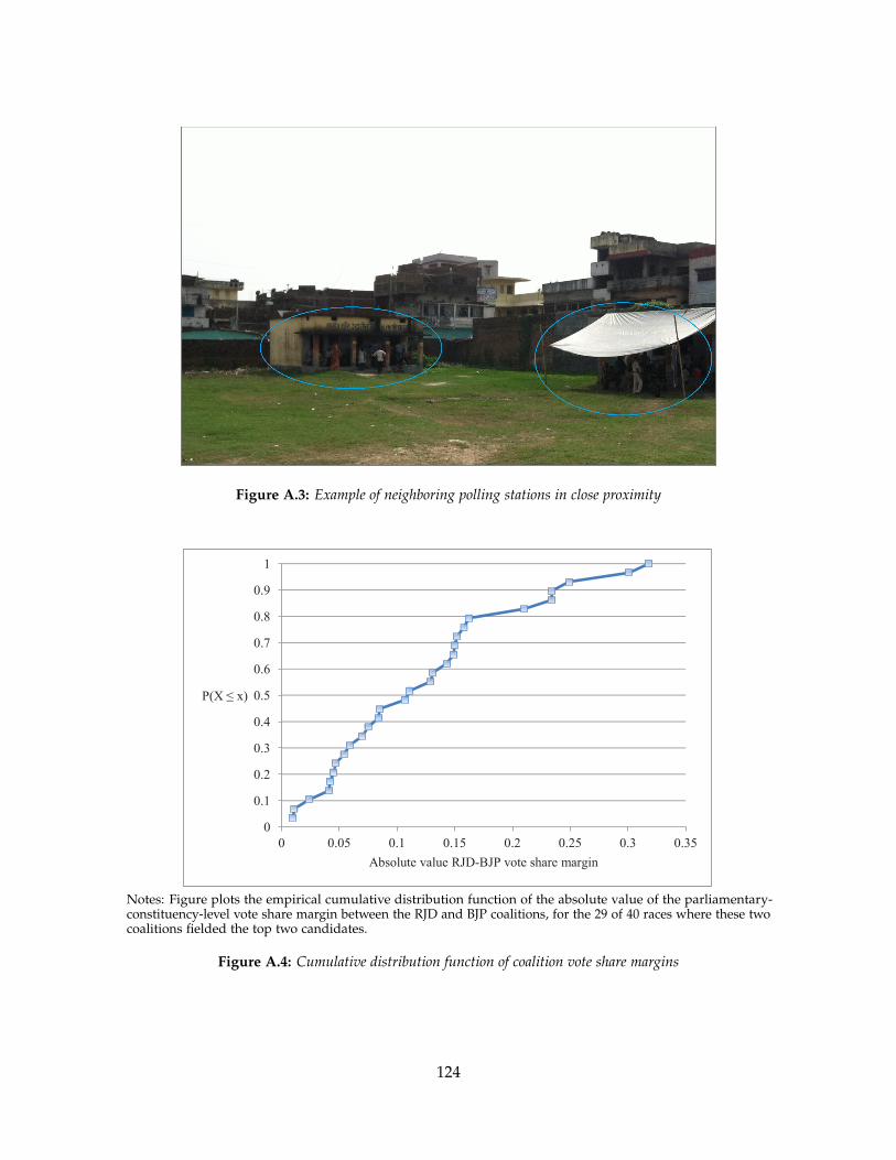
Figure A.3: Example of neighboring polling stations in close proximity

0

0.1

0.2

0.3

0.4

0.5

0.6

0.7

0.8

0.9

1

0 0.05 0.1 0.15 0.2 0.25 0.3 0.35

P(X ≤ x)

Absolute value RJD-BJP vote share margin

Notes: Figure plots the empirical cumulative distribution function of the absolute value of the parliamentary-constituency-level vote share margin between the RJD and BJP coalitions, for the 29 of 40 races where these twocoalitions fielded the top two candidates.

Figure A.4: Cumulative distribution function of coalition vote share margins

124

Table A.1: Randomization check - spatial characteristics

Homog. Mixedteam team Difference p-value Obs.

(1) (2) (3) (4) (5)

Number mixed team neighbor stations 0.385 0.386 -0.012 0.493 5,561[0.746] [0.719] (0.018)

Total neighbor stations 1.200 1.191 -0.027 0.420 5,561[1.614] [1.647] (0.034)

Number mixed team stations 0.420 0.452 0.026 0.392 5,097within 0.25km [1.078] [1.159] (0.030)

Number mixed team stations 2.536 2.622 0.066 0.430 5,097within 0.25-0.75km [4.263] [4.470] (0.084)

Total stations within 0.25km 1.357 1.336 -0.025 0.735 5,097[2.930] [2.904] (0.073)

Total stations within 0.25-0.75km 7.893 7.958 0.069 0.768 5,097[12.830] [12.904] (0.232)

Number mixed team stations 1.210 1.309 0.043 0.607 3,231within village [2.178] [2.287] (0.083)

Number mixed team stations 4.688 4.829 -0.040 0.768 3,216in neighboring villages [3.908] [4.015] (0.136)

Total stations within village 3.686 3.812 0.088 0.676 3,231[5.551] [5.868] (0.212)

Total stations in neighboring villages 14.259 14.479 0.065 0.861 3,216[10.694] [10.544] (0.369)

Notes: Columns (1) and (2) report variable means with standard deviations in brackets for homogeneous andmixed officer teams. Column (3) reports the coefficient from an OLS regression where the listed outcome isregressed on an indicator for polling station mixed team composition and column (4) reports the associatedp-value. Also included are sub-constituency and number of officer fixed effects. Neighbor stations are pollingstations within the same building/compound of a given polling station. Stations with 0.25 and within 0.25-0.75km are non-neighbor stations within 0.25km and 0.25-0.75km of a given polling station, respectively.Numbers of stations within a village and in neighboring villages are the numbers of non-neighbor pollingstations within the same village as a given polling station and in villages adjacent to a given polling station’svillage, respectively. Sample is restricted to those polling stations matched to the dataset of polling station GPSlocations. Village-related outcomes further exclude stations in villages which are in the top 1 percent of thedistribution in terms of number of polling stations contained within, or their neighboring villages.*Significant at10% level **5% level ***1% level.

125

Table A.2: Cross-position balance

Presiding Polling Polling Polling Pollingofficer officer 1 officer 2 officer 3 officer 4

(1) (2) (3) (4) (5)

Muslim/Yadav presiding officer -0.006 0.006 -0.004 -0.016(0.014) (0.014) (0.014) (0.030)

Muslim/Yadav polling officer 1 -0.005 -0.004 -0.019 -0.015(0.013) (0.013) (0.013) (0.027)

Muslim/Yadav polling officer 2 0.006 -0.004 0.014 -0.009(0.014) (0.014) (0.015) (0.027)

Muslim/Yadav polling officer 3 -0.003 -0.018 0.012 -0.020(0.013) (0.012) (0.014) (0.029)

Muslim/Yadav polling officer 4 -0.014 -0.013 -0.009 -0.017(0.026) (0.030) (0.031) (0.025)

Observations 5,561 5,561 5,561 5,523 1,178Notes: Each column reports coefficients from an OLS regression where the outcome is Muslim/Yadav assignmentto the specified position, and is regressed on dummies for Muslim/Yadav assignment to the other polling officerteam positions specified in table. Additionally included are sub-constituency and number of officer fixed effects.*Significant at 10 percent. **Significant at 5 percent. ***Significant at 1 percent.

126

Table A.3: Position- and number-specific impacts on voting outcomes



Panel A. PositionMuslim/Yadav presiding officer -0.006 -0.017 0.007 -0.012

(0.052) (0.043) (0.020) (0.018)Muslim/Yadav polling officer 1 0.088* -0.013 0.031* 0.017

(0.050) (0.037) (0.019) (0.011)Muslim/Yadav polling officer 2 0.050 -0.064 0.021 0.002

(0.052) (0.044) (0.020) (0.014)Muslim/Yadav polling officer 3 0.054 -0.086** 0.037* 0.000

(0.050) (0.040) (0.019) (0.019)Muslim/Yadav polling officer 4 0.111 -0.001 0.041 0.001

(0.189) (0.170) (0.087) (0.033)F-test p-value: equality of coeffs. 0.731 0.612 0.824 0.614Observations 5,276 5,290 5,293 5,293

Panel B. NumberAny Muslim/Yadav officer 0.055* -0.046** 0.027** 0.002

(0.028) (0.022) (0.011) (0.008)Multiple Muslim/Yadav officers -0.061 0.040 -0.024 -0.010

(0.061) (0.053) (0.024) (0.018)Observations 5,535 5,535 5,549 5,549

Notes: All columns in Panel A report OLS estimates from regressions at the polling station level of the listedvariable on indicators for Muslim/Yadav presence in each polling party position, conditional on there being 1 orfewer total MY officers at the polling station. All columns in Panel B report OLS estimates from regressions at thepolling station level of the listed variable on indicators for the degree of Muslim/Yadav presence. Additionallyincluded in all regressions are sub-constituency and number of officer fixed effects and controls for the lognumber of registered voters at the polling station and the Muslim/Yadav share of registered voters *Significantat 10 percent. **Significant at 5 percent. ***Significant at 1 percent.

127

Table A.4: Heterogeneity in impacts of team composition by electorate composition



Mixed team 0.038 -0.023 0.018 0.003(0.037) (0.027) (0.014) (0.010)

Mixed team * Muslim/Yadavregistered voter % 0.057 -0.131 0.039 -0.014

(0.158) (0.166) (0.053) (0.039)

Muslim/Yadav registered voter % 0.031*** -0.029*** 0.015*** -0.000*(0.001) (0.001) (0.000) (0.000)

Observations 5,535 5,549 5,552 5,552Notes: Each column reports OLS estimates from regressions at the polling station level of the listed outcomeon indicators for mixed team composition, interacted with a continuous measure of the polling station levelproportion of registered voters that are Muslim or Yadav. Additionally included are sub-constituency andnumber of officer fixed effects and a control for log total registered voters. *Significant at 10 percent. **Significantat 5 percent. ***Significant at 1 percent.

128

Table A.5: Cross-station spillovers - extended range



Panel A. Buffer radiusMixed team composition 0.062** -0.060*** 0.033** -0.001

(0.028) (0.022) (0.011) (0.008)Number mixed team neighbor 0.024 -0.049** 0.026*** -0.001stations (0.026) (0.020) (0.010) (0.008)

Number mixed team stations 0.012 0.014 -0.006 -0.004within 0.25km (0.026) (0.014) (0.009) (0.007)

Number mixed team stations -0.006 0.005 -0.003 0.000within 0.25-0.75km (0.009) (0.008) (0.004) (0.002)

Total neighbor stations -0.028** 0.028*** -0.021*** -0.011***(0.013) (0.010) (0.005) (0.003)

Total stations within 0.25km -0.028** 0.007 -0.007** -0.006**(0.011) (0.006) (0.003) (0.003)

Total stations within 0.25-0.75km 0.001 0.007*** -0.003* 0.001(0.004) (0.003) (0.001) (0.001)

Observations 5,074 5,087 5,090 5,090Number locations 3,307 3,307 3,307 3,307Panel B. Village boundariesMixed team composition 0.083** -0.070** 0.037** 0.010

(0.038) (0.031) (0.015) (0.010)Number mixed team neighbor 0.069 -0.108*** 0.048** 0.011stations (0.054) (0.041) (0.019) (0.011)

Number mixed team stations -0.017 -0.044 0.010 -0.003within village (0.039) (0.029) (0.016) (0.008)

Number mixed team stations 0.008 -0.020* 0.009 0.004in neighboring villages (0.013) (0.011) (0.006) (0.003)

Total neighbor stations -0.033 0.102*** -0.044*** -0.001(0.033) (0.026) (0.012) (0.010)

Total stations within village 0.016 0.016 -0.004 -0.000(0.019) (0.013) (0.007) (0.003)

Total stations in neighboring 0.000 0.011** -0.004* 0.000villages (0.005) (0.004) (0.002) (0.001)

Observations 3,196 3,210 3,212 3,212Number villages 1,247 1,247 1,247 1,247

Notes: Each column within a panel reports OLS estimates from a regression at the polling station level of thelisted variable on an indicator for mixed team composition. Each regression includes sub-constituency andnumber of officer fixed effects and controls for log total registered voters and share Muslim/Yadav registeredvoters. Neighbor stations are those within the same building/compound of a given polling station. Stationswithin 0.25 and 0.25-0.75km are non-neighbor stations within the stated distance of a given polling station.Numbers of stations within a village and in neighboring villages are the numbers of non-neighbor pollingstations within the same village as a given station and in villages adjacent to a given station’s village. PanelA is restricted to stations matched to the dataset of station GPS locations. Panel B further excludes stationsin the top 1 percent of villages in terms of number of stations contained within, or their neighboring villages.*Significant at 10 percent. **Significant at 5 percent. ***Significant at 1 percent.

129

Table A.6: Type-specific impacts of officer identity on voting outcomes



Any Muslim officer 0.051* -0.034 0.023** 0.011(0.030) (0.024) (0.012) (0.008)

Any Yadav officer 0.070 -0.100** 0.044** -0.033(0.057) (0.044) (0.022) (0.025)

Muslim/Yadav registered voter % 0.031*** -0.030*** 0.015*** -0.000**(0.001) (0.001) (0.000) (0.000)

Ln total electors 1.007*** 1.198*** -0.069*** 0.934***(0.062) (0.050) (0.024) (0.019)

Control Mean [SD] 4.451 5.143 -0.181 6.180[1.198] [0.969] [0.452] [0.402]

Observations 5,276 5,290 5,293 5,293Notes: All columns report OLS estimates from regressions at the polling station level of the listed variable onindicators for Muslim and Yadav presence, conditional on there being 1 or fewer total Muslim/Yadav officersat the polling station. Additionally included are sub-constituency and number of officer fixed effects andcontrols for Muslim/Yadav share of registered voters and log total registered voters. *Significant at 10 percent.**Significant at 5 percent. ***Significant at 1 percent.

130

Table A.7: Cross-election impacts of randomized team composition on voting outcomes


RJD BJP RJD-BJP votes2015 2015 2015 2015(1) (2) (3) (4)

Mixed team -0.016 -0.012 0.001 0.004(0.043) (0.043) (0.020) (0.012)

Number mixed team neighbor stations 0.005 -0.067 0.035 0.025(0.058) (0.058) (0.025) (0.015)

Total number neighbor stations -0.107*** -0.011 -0.045*** -0.054***(0.036) (0.043) (0.015) (0.009)

Muslim/Yadav elector % 0.020*** -0.026*** 0.013*** 0.000(0.001) (0.002) (0.000) (0.000)

Ln total electors 0.969*** 0.858*** 0.015 0.819***(0.146) (0.147) (0.062) (0.047)

Observations 1,335 1,332 1,335 1,335Number locations 1,008 1,007 1,008 1,008Homogeneous team mean [SD] 5.096 5.106 -0.010 6.243

[0.908] [0.973] [0.433] [0.321]Notes: All columns report OLS estimates from regressions at the polling station level of the listed variable fromthe 2015 elections on an indicator for mixed team composition and variables for the numbers of total and mixedcomposition team neighboring polling stations in the 2014 elections. Additionally included are AC and numberof officer fixed effects and controls for Muslim/Yadav share of registered voters and log total registered votersfrom 2014. Neighbor stations are polling stations within the same location (building/compound) as a givenpolling station. Standard errors clustered at the location level. The sample is restricted to the district where onlyminor changes were made to the polling station locations between the 2014 and 2015 elections. *Significant at 10percent. **Significant at 5 percent. ***Significant at 1 percent.

131

Appendix B


132

Table B.1: Differential initial trends check

State levelDifference inlog contract

value(1)

Panel A. IndiaE-procurement 0.0130

(0.0378)Mean Dep. Var. 0.202

(0.697)Observations 24Panel B. Indonesia - Works ProjectsE-procurement (IV) -0.084

(0.115)Mean Dep. Var. 0.086

(0.490)Observations 24Panel C. Indonesia - Consultancy ProjectsE-procurement (IV) 0.017

(0.235)Mean Dep. Var. -0.576

(0.790)Observations 21

Notes: India - Column (1) reports an OLS estimate at the state level, where the dependent variable is thedifference in log average contract value between 2000 and 2001. The independent variable is the year of officialadoption of electronic procurement at the state level, conditional on adoption occurring after 2001. Indonesia -Column (1) reports OLS estimates at the state level, where the dependent variable is the difference in log averagecontract value between 2005 and 2004. The independent variable is the year of official adoption of electronicprocurement at the state level, conditional on adoption occurring after 2005. Robust standard errors are inparentheses below estimates. Non-e-procurement project means for each dependent variable are also reported,with standard deviations in parentheses. *Significant at 10 percent. **Significant at 5 percent. ***Significant at 1percent.

133

Appendix C


134

Table C.1: Candidate entry

Non-Number incumbent Incumbent

candidates present present(1) (2) (3)

Open meetings * Capital isolation -0.106 0.126 0.015(0.241) (0.159) (0.119)

Open meetings 0.041 -0.100 0.007(0.165) (0.105) (0.075)

Observations 89,347 89,347 89,347

Effect: mean sample isolation -0.032 -0.013 0.018(0.030) (0.020) (0.014)

Effect: min sample isolation -0.004 -0.047 0.014(0.067) (0.041) (0.027)

Effect: max sample isolation -0.049 0.007 0.020(0.051) (0.036) (0.029)

Outcome mean [SD] 1.775 0.730 0.769[0.621] [0.444] [0.421]

State, Region*Year FE X X XLegislative controls X X XPopulation/income controls X X X

Notes: All columns report OLS estimates from regressions at the state level of the listed variable on an indicatorfor open meetings interacted with state capital isolation as of 1950. Regressions include district and period-by-census-region fixed effects and, in addition to those listed in Table 3.2, controls for shares of the population age18 and older. Standard errors clustered at the state level. Additionally shown in each column are the impliedeffects of open meetings at the average 1950 level of isolation observed in the data across states, as well as theminimum and maximum values. *Significant at 10 percent. **Significant at 5 percent. ***Significant at 1 percent.

135

essays in economic development and political economy

Documents