1

Name:_____solution____

ESE 403

Operations Research

Fall 2010

Examination 2

Closed book/notes/homework/cellphone examination. You may use a calculator. Please

write on one side of the paper only. Extra pages will be supplied upon request.

You will only receive full credit if you show all your work.

Question Point value Your Score

1 20

2 20

3 20

4 20

5 20

Total 100

2

1. (20 points) Consider the following problem.

Maximize Z = 4x1 + 3x2 + 6x3

Subject to

3x1 + x2 + 3x3 ≤ 30

2x1 +2x2 + 3x3 ≤ 40

and

x1, x2, x3 ≥0

Solve using REVISED Simplex method in MATRIX form using the following equations. Show all

steps.

3

� � � �� � ��, � � � � �� � � , b = ����

Initialization:

�� � � ���� � � ���� , �� �� �� ��, � � � � �� � � ���

Optimality test:

����� � � � � �� � �� � �� � �� � ��� �� ���, not optimal

Iteration 1:

Pick x3 to enter, ��� � � � �� � � , minimum ratio test ��� � ��

� , pick x4 to leave

� �� ����� , ��� � ��� ��� � � �� � � ��� ��� �

�� � ���� � ���� � ��� ��� � ���� � ���� � ������������� � �� ��

Optimality test:

����� � � � � �� �� ��� ��� � � � �� � � � �� � �� � �� �� ��, not optimal

Iteration 2:

x2 to enter, ��� � ��� ��� � � � �� � � � � ��� �� � � , minimum ratio test ��� � ��

��� pick x5 to leave

� �� ����� , ��� � � ����� � ��� ��� � � ��� ������ �

�� � ���� � ���� � ��� ������ � ���� � ������ � ������������� � �� ��

Optimality test:

����� � � � � �� �� �� ����� � ! � � �� � � � �� � �� ������������������������ � �� �� � � �� � � � �� � �� ������������������������ � �" � �� � �� � �� �� �� � �� optimal

4

2. (20 points) Consider the following problem

Maximize Z = 2x1 - x2 + x3

Subject to

3x1 + x2 + x3 ≤ 6

x1 - x2 + 2x3 ≤ 1

x1 + x2 - x3 ≤ 2

x1, x2, x3 ≥0

a. Construct the dual problem for this primal problem

b. Solve the DUAL problem using DUAL SIMPLEX METHOD in tabular form. Show all steps.

Minimize W = 6y1 + y2 + 2y3

Subject to

3y1 + y2 + y3 ≥ 2

y1 - y2 + y3 ≥ -1

y1 + 2y2 - y3 ≥ 1

y1, y2, y3 ≥0

which is equal to:

Maximize (-W) = -6y1 - y2 - 2y3

Subject to

-3y1 - y2 - y3 ≤ -2

-y1 + y2 - y3 ≤ 1

-y1 - 2y2 + y3 ≤ -1

y1, y2, y3 ≥0

5

y1 y2 y3 y4 y5 y6 RHS

Z=-W 6 1 2 0 0 0 0

y4 -3 -1 -1 1 0 0 -2

y5 -1 1 -1 0 1 0 1

y6 -1 -2 1 0 0 1 -1

y1 y2 y3 y4 y5 y6 RHS

Z=-W 3 0 1 1 0 0 -2

y2 3 1 1 -1 0 0 2

y5 -4 0 -2 1 1 0 -1

y6 5 0 3 -2 0 1 3

y1 y2 y3 y4 y5 y6 RHS

Z=-W 1 0 0 1.5 0.5 0 -2.5

y2 1 1 0 -0.5 0.5 0 1.5

y3 2 0 1 -0.5 -0.5 0 0.5

y6 -1 0 0 -0.5 1.5 1 1.5

Optimal object function of 2.5 at y1=0, y2=1.5, y3=0.5

6

3. (20 points) Consider the following problem

Maximize Z = 7x1 + 2x2 - 3x3

Subject to

4x1 + x2 - x3 ≤ 10

3x1 + x2 + 4x3 ≤ 30

x1, x2, x3 ≥0

by letting x4 and x5 be the slack variables for the respective constraints, the Simplex method yield the

following final set of equations:

(0) Z + x1 + x3 + 2x4 = 20

(1) 4x1 +x2 - x3 + x4 = 10 (also acceptable if use 4x1 +x2 + x3 + x4 = 10)

(2) – x1 + 5x3 – x4 + x5 = 20

Now you are to consuct sensitivity analysis by independently investigating each of the following changes

in the original model. For each change, use the sensitivity analysis procedure to revise this set of

equations (in tableau form) and convert it to proper form from Gaussian elimination for identifying and

evaluating the current basic solution. Then test this solution for feasibility and for optimality. If either

test fails, reoptimize to find a new optimal solution.

a. Change the right-hand sides to b1 = 30, b2=20

b. Change the coefficient of x3 to c3 = -2, a13 = -2, a23 = 3

c. Change the coefficient of x2 to c2 = 4, a12 = 2, a22 = 3

d. Change the objective function to Z = 5x1 + x2 -2x3

e. Introduce a new constraint 2x1 + 3x2 + 3x3 ≤ 25.

Final tableau

x1 x2 x3 x4 x5 RHS

Z 1 0 1 2 0 20

x2 4 1 -1 1 0 10

x5 -1 0 5 -1 1 20

7

a. ∆b1 = 20, ∆b2 = -10

∆Z*= �� �� ����� = 40

∆b1*= �� �� ����� = 20

∆b1*= ��� �� ����� = -30

Revised Final Tableau

x1 x2 x3 x4 x5 RHS

Z 1 0 1 2 0 60

x2 4 1 -1 1 0 30

x5 -1 0 5 -1 1 -10

The current basic solution is superoptimal, but infeasible, apply dual simplex method to reoptimize

x1 x2 x3 x4 x5 RHS

Z 0 0 6 1 1 50

x2 0 1 19 -3 4 -10

x1 1 0 -5 1 -1 10

x1 x2 x3 x4 x5 RHS

Z 0 0.333333 12.33333 0 2.333333 46.66667

x4 0 -0.33333 -6.33333 1 -1.33333 3.333333

x1 1 0.333333 1.333333 0 0.333333 6.666667

b. ∆a13 = -1, ∆a23 = -1

∆c3 = 1 → ∆(z*

3 – c3) = -1 + #� �$ %����& � ���

∆a*

13 = #� �$ %����& � ��

∆a*

23 = #� ��$ %����& � �

Revised Final Tableau

x1 x2 x3 x4 x5 RHS

Z 1 0 -2 2 0 20

x2 4 1 -2 1 0 10

x5 -1 0 5 -1 1 20

8

The current basic solution is feasible, but suboptimal, apply simplex method to reoptimize

x1 x2 x3 x4 x5 RHS

Z 0.6 0 0 1.6 0.4 28

x2 3.6 1 0 0.6 0.4 18

x3 -0.2 0 1 -0.2 0.2 4

d. ∆c1 = -2 → ∆(z*

1-c1) = 2

∆c2 = -1 → ∆(z*

2-c2) = 1

∆c3 = 1 → ∆(z*

3-c3) = -1

Revised final tableau:

x1 x2 x3 x4 x5 RHS

Z 3 1 0 2 0 20

x2 4 1 -1 1 0 10

x5 -1 0 5 -1 1 20

Revised final tableau after converting to proper form

x1 x2 x3 x4 x5 RHS

Z -1 0 1 1 0 10

x2 4 1 -1 1 0 10

x5 -1 0 5 -1 1 20

The current basic solution is feasible, but not optimal

x1 x2 x3 x4 x5 RHS

Z 0 0.25 0.75 1.25 0 12.5

x1 1 0.25 -0.25 0.25 0 2.5

x5 0 0.25 4.75 -0.75 1 22.5

e. New tableau

x1 x2 x3 x4 x5 x6 RHS

Z 1 0 1 2 0 0 20

x2 4 1 -1 1 0 0 10

x5 -1 0 5 -1 1 0 20

x6 2 3 3 0 0 1 25

9

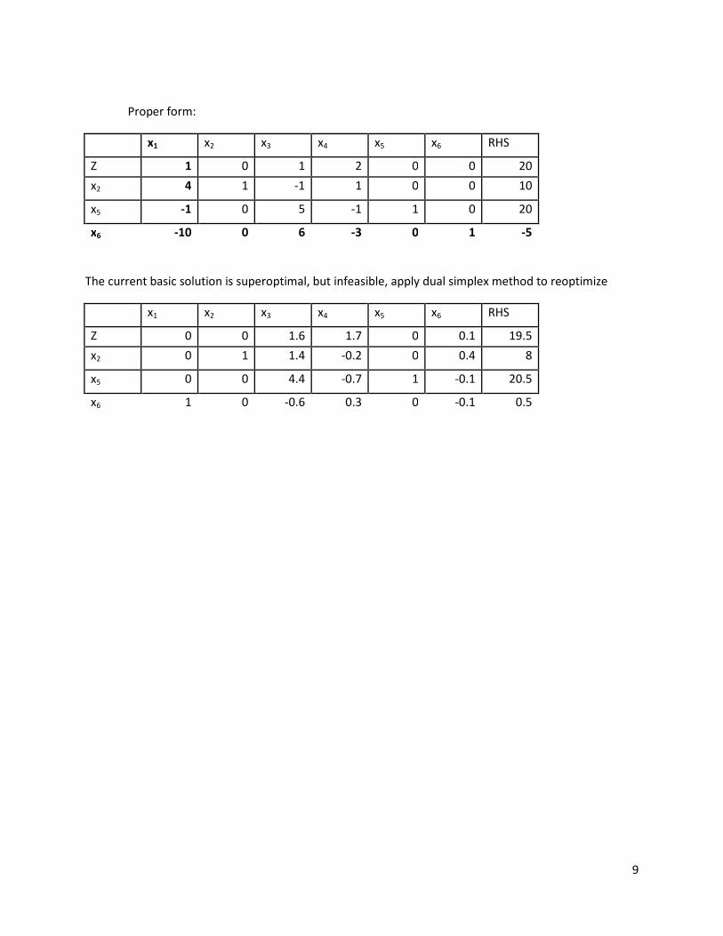
Proper form:

x1 x2 x3 x4 x5 x6 RHS

Z 1 0 1 2 0 0 20

x2 4 1 -1 1 0 0 10

x5 -1 0 5 -1 1 0 20

x6 -10 0 6 -3 0 1 -5

The current basic solution is superoptimal, but infeasible, apply dual simplex method to reoptimize

x1 x2 x3 x4 x5 x6 RHS

Z 0 0 1.6 1.7 0 0.1 19.5

x2 0 1 1.4 -0.2 0 0.4 8

x5 0 0 4.4 -0.7 1 -0.1 20.5

x6 1 0 -0.6 0.3 0 -0.1 0.5

10

4. (20 points) Consider the following problem.

Maximize Z = 3x1 + 4x2 + 8x3

subject to

2x1 + 3x2 + 5x3 ≤ 9

x1 + 2x2 + 3x3 ≤ 5

and

x1 ≥ 0, x2 ≥ 0, x3 ≥ 0.

Let x4 and x5 denote the slack variables for the respective functional constraints. After we apply the

Simplex method, the final simplex tableau is

Coefficient of:

Basic

Variable

Eq.

Z

x1

x2

x3

x4

x5

Right

Side

Z (0) 1 0 1 0 1 1 14

x1 (1) 0 1 -1 0 3 -5 2

x3 (2) 0 0 1 1 -1 2 1

Find the allowable ranges for c1, c2, c3, b1, and b2

11

x2 is a nonbasic variable, so the allowable range can be found by

y*A –c ≥0,

c2 ≤ y*A2 = �� �� �� = 5, c1 ≤ 5

x1, and x3 are basic variables

-∆c1 ≥ -1, ∆c1 ≤ 1

3∆c1 ≥ -1, ∆c1 ≥ -1/3

-5∆c1 ≥ -1, ∆c1 ≤ 1/5

Therefore, -1/3 ≤ ∆c1 ≤ 1/5, 2 2/3 ≤ c1 ≤ 3 1/5

-∆c3 ≥ -1, ∆c3 ≤ 1

-∆c3 ≥ -1, ∆c3 ≤ 1

2∆c3 ≥ -1, ∆c3 ≥ -1/2

Therefore, -1/2 ≤ ∆c3 ≤ 1, 7 1/2 ≤ c3 ≤ 9

�� ' � �"�� � ()�� * �� �� ' +�()��()�, * �

2+3∆b1 ≥ 0, ∆b1 ≥ -2/3

1 - ∆b1 ≥ 0, ∆b1 ≤ 1

Therefore, -2/3 ≤ ∆b1 ≤ 1, 8 1/3 ≤ b1 ≤ 10

�� ' � �"�� � + �()�, * �� �� ' +�"()��()� , * �

2-5∆b2 ≥ 0, ∆b2 ≤ 2/5

1 + 2∆b2 ≥ 0, ∆b2 ≥ -1/2

Therefore, -1/2 ≤ ∆b2 ≤ 2/5, 4 1/2 ≤ b2 ≤ 5 2/5

12

5. (20 points) Use parametric linear programming to find the optimal solution for the following

problem as a function of θ, for 0 ≤ θ ≤ 20

Maximize Z = (20+4θ)x1 + (30-3θ)x2 + 5x3

subject to

3x1 + 3x2 + x3 ≤ 10

8x1 + 6x2 + 4x3 ≤ 25

6x1 + x2 + x3 ≤ 15

and

x1 ≥ 0, x2 ≥ 0, x3 ≥ 0.

x1 x2 x3 x4 x5 x6 RHS

Z -20 -30 5 0 0 0 0

x4 3 3 1 1 0 0 10

x5 8 6 4 0 1 0 25

x6 6 1 1 0 0 1 15

x1 x2 x3 x4 x5 x6 RHS

Z 10 0 15 10 0 0 100

x2 1 1 1/3 1/3 0 0 10/3

x5 2 0 2 -2 1 0 5

x6 5 0 2/3 -1/3 0 1 35/3

x1 x2 x3 x4 x5 x6 RHS

Z 10-4θ 3θ 15 10 0 0 100

x2 1 1 1/3 1/3 0 0 10/3

x5 2 0 2 -2 1 0 5

x6 5 0 2/3 -1/3 0 1 35/3

x1 x2 x3 x4 x5 x6 RHS

Z 10-7θ 0 15-θ 10-θ 0 0 100-10θ

x2 1 1 1/3 1/3 0 0 10/3

x5 2 0 2 -2 1 0 5

x6 5 0 2/3 -1/3 0 1 35/3

x1 x2 x3 x4 x5 x6 RHS

Z 0 0 (55- θ)/15 (160-22 θ)/15 0 (-10+7 θ)/5 (230+19 θ)/3

x2 0 1 1/5 2/5 0 -1/5 1

x5 0 0 26/15 -28/15 1 -2/5 1/3

x1 1 0 2/15 -1/15 0 1/5 7/3

x1 x2 x3 x4 x5 x6 RHS

Z 0 (-80+11θ)/3 (-5+2 θ)/3 0 0 (10+2 θ)/3 50+10 θ

x4 0 5/2 ½ 1 0 -1/2 5/2

x5 0 14/3 8/3 0 1 -4/3 5

x1 1 1/6 1/6 0 0 1/6 5/2

For 0 ≤ θ ≤ 10/7, (x1, x2, x3, x4, x5) = (0, 10/3, 0, 0, 5, 35/3) with optimal objective function value: 100-10θ

For 10/7 ≤ θ ≤ 80/11, (7/3, 1, 0, 0, 1/3, 0) with optimal objective function value: (230+19θ)/3

For 80/11 ≤ θ, (5/2, 0, 0, 5/2, 5, 0) with optimal objective function value: 50+10θ