By Michael Kane

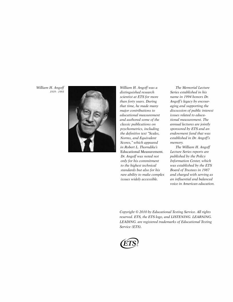
William H. Angoff1919 - 1993

William H. Angoff was a distinguished research scientist at ETS for more than forty years. During that time, he made many major contributions to educational measurement and authored some of the classic publications on psychometrics, including the definitive text “Scales, Norms, and Equivalent Scores,” which appeared in Robert L. Thorndike’s Educational Measurement. Dr. Angoff was noted not only for his commitment to the highest technical standards but also for his rare ability to make complex issues widely accessible.

The Memorial Lecture Series established in his name in 1994 honors Dr. Angoff’s legacy by encour-aging and supporting the discussion of public interest issues related to educa-tional measurement. The annual lectures are jointly sponsored by ETS and an endowment fund that was established in Dr. Angoff’s memory.

The William H. Angoff Lecture Series reports are published by the Policy Information Center, which was established by the ETS Board of Trustees in 1987 and charged with serving as an influential and balanced voice in American education.

Copyright © 2010 by Educational Testing Service. All rights reserved. ETS, the ETS logo, and LISTENING. LEARNING. LEADING. are registered trademarks of Educational Testing Service (ETS).

Errors of MEasurEMEnt, thEory, and Public Policy

Michael Kane

ETS Samuel J. Messick Chair in Test Validity

(Formerly Director of Research, National Conference of Bar Examiners, Madison, WI)

ETS

Policy Evaluation and Research Division

Policy Information Center

Princeton, NJ 08541-0001

The 12th annual William H. Angoff Memorial Lecture was presented at Educational Testing Service, Princeton, New Jersey, on November 19, 2008.

2 3

Preface

The 12th annual William H. Angoff Memorial Lecture was presented by Dr. Michael T. Kane, ETS’s Samuel J. Messick Chair in Test Validity and the former Director of Research at the National Confer-ence of Bar Examiners. Dr. Kane argues that it is important for policymakers to recognize the impact of errors of measurement on test scores and on average scores for groups. He asserts that a clear understanding of the magnitude of errors of measurement can have at least two benefits: identifying where measurement procedures need to be improved, and improving policy decisions by reducing the tendency to interpret and act on score differences that may, in fact, be meaningless.

Dr. Kane grounds his argument in a discussion of the origins of errors of measurement, their role in conceptual frameworks and their control. He then discusses the relationship between defini-tions of constructs (variables of interest) and our conception of errors of measurement. Understanding this relationship helps users of test scores decide whether a score difference should be interpreted as a difference in the construct being measured or should be attributed to error.

Given the increasing reliance on assessments in high-stakes educational decisions, Dr. Kane’s cogent discussion is very timely.

The William H. Angoff Memorial Lecture Series was established in 1994 to honor the life and work of Bill Angoff, who died in January 1993. For more than 50 years, Dr. Angoff made major contributions to educational and psychological measurement and was deservedly recognized by the major societies in the field. In line with Dr. Angoff’s interests, this lecture series is devoted to relatively nontechnical discussions of important public interest issues related to educational measurement.

Ida Lawrence Senior Vice President ETS Research & Development January 2010

2 3

acknowledgments

In addition to the lecturer’s scholarship and commitment in the presentation of the annual William H. Angoff Memorial Lecture and the preparation of this publication, ETS Research and Development would like to acknowledge Barb Schmidt for administrative arrangements, Kim Fryer and Eileen Ker-rigan for editorial support and Sally Acquaviva for production assistance. Most importantly, we are grateful to Eleanor Angoff for her continued support of the lecture series.

abstract

Errors of measurement arise because our observations are affected by many sources of variability, but our conceptual frameworks necessarily ignore much of this variability. Sources of variability that are not included in our models and descriptions of phenomena are treated as error or noise. A good theory of error supports the development of precise measurements, clearly defined constructs and sound pub-lic policy. Narrowly defined constructs that do not generalize much beyond the observed performances do not involve many sources of error, but constructs that generalize observed scores over a broad range of conditions of observation (e.g., context, time, test tasks) necessarily involve many potential sources of error. We can have narrow constructs with small errors or more broadly defined constructs with larger errors. Some errors that are negligible for individuals can have a substantial impact on estimates of group performance, and therefore, can have serious consequences.

4 5

Error is a delicate concept; for if we can call on it at will, or willfully, then it no longer explains anything or ac-counts for anything. And if we can’t call on it when we need it, none of our theories ... will stand up. (Kyburg, 1968, p. 140)

I am greatly honored to have been invited to participate in this lecture series in honor of Bill Angoff. I did not know him well, but I have ad-mired his work for its acute sense of the questions that needed to be asked and for its insightful anal-yses of basic measurement issues.

In this tradition and in memory of Dr. An-goff, I intend to review some basic assumptions about errors of measurement. Dr. Angoff was very careful about his assumptions, and my discussion will try to follow in that tradition by examining how errors of measurement arise and how they are used. My presentation will focus on several closely related themes.

First, I will talk about the origins of er-rors of measurement, their role in our conceptual frameworks and their control. Without some sense of what to expect in a set of observations, there is no reason to assume that our observations contain any errors of measurement. It is only when scores that should agree do not agree, that the notion of

errors of measurement gets called into play. Ironi-cally perhaps, errors of measurement presuppose clearly defined measurement procedures and at least some rudimentary theory before they can even be recognized.

Second, I will consider the relationship be-tween how we define our constructs (the variables of interest) and our conception of errors of mea-surement. Ultimately, we get to decide whether a score difference should be taken seriously as a difference in the construct of interest or should be attributed to error. Broadly defined constructs, which generalize over a wide range of conditions of observation, tend to have more errors than nar-rowly defined constructs, which do not go much beyond the observations actually made.

Third, I will talk a bit about how errors of measurement function in various policy contexts. A clear recognition of the impact of errors on test scores and on average scores for groups can im-prove policy decisions by encouraging a salutary sense of uncertainty. A good sense of the magni-tude of errors of measurement at different levels of analysis can highlight sources of error that merit special attention because of their consequences, and can lessen the temptation to interpret and act on meaningless differences.

IntroductIon

4 5

aradoxically, errors of measurement do not ex-ist, but they are essential. As illustrated below, there is nothing about a single test score or a pair of scores that implies the presence of errors of measurement. However, if two scores are taken to be measures of the same variable for the same per-son, we expect them to be equal, and if they are not equal, our data are inconsistent with our con-ceptual framework. We can resolve this dilemma by assuming that one or both of the measurements contain errors. Errors of measurement play a vital role in quantitative analyses, by making it possible to model data without immediately running into inconsistencies.

The Need for errors of MeasureMeNT

To take a simple example, suppose that we have made observations of the performance of four students, Alex, Beth, Chad and Dan, on some tasks (e.g., on a multiple-choice or performance test) and found that the four students got scores of 65, 77, 79 and 49, respectively. At this point, there is no reason to assume that these scores con-tain any errors of measurement. They are what they are!

Assuming that no mistakes were made in observing the performances or in reporting the scores, we are justified in accepting the scores at face value as summaries of the observed perfor-mances. That Alex got a score of 65, Beth got a score of 77, Chad got a score of 79 and Dan got a score of 49 can be considered facts. To ask about what the scores might have been if the four

students had performed a different set of tasks or had performed the tasks on a different day or in a different context is to ask about hypothetical outcomes; in fact, the students performed those tasks on that day and in that context and got scores of 65, 77, 79 and 49. Similarly, it is a fact (or, if one wants to be very proper about it, a valid mathematical inference from the scores) that, on that occasion, Chad got a higher score than Beth, who got a higher score than Alex, who got a higher score than Dan. Taken as reports of events as they occurred, none of these scores contains any error. The students performed as they did, and they were correctly awarded the reported scores.

Now, suppose that on the next day, we obtain new observations of the same four students using the same procedures, and we find that Alex gets a score of 69, Beth gets a score of 80, Chad gets a score of 75 and Dan gets a score of 46. The scores are different on the two days and their order is a bit different, but there is nothing incon-sistent in getting different scores on different days. These differences do not, in themselves, force us to introduce the notion of errors of measurement.

In fact, we have a range of options for de-scribing the changes in the scores from one day to another. First, we can interpret each student’s score for each day as characterizing that student’s performance on that day. The score is reported for each student on each day, and the scores can vary from student to student and day to day. In some cases we might expect the scores to change from day to day. For example, we might expect a

errors of measurement and theIr control

P

6 7

student’s level of skill in an activity to improve, over time, as a function of instruction and prac-tice. If the scores were derived from measures of an attribute that is likely to change from day to day or week to week, we would be concerned about the sensitivity of our instrument if we did not see any changes in scores.

In some contexts, we might expect perfor-mance to vary as a function of time, but not nec-essarily to follow a particular trend. If we assume that the attribute is likely to change from one ob-servation to the next, because of fluctuations in the attribute (e.g., attitudes, moods), changes in a person’s scores from day to day are likely to be in-terpreted as changes in the attribute of interest.

However, in some cases, it may be reason-able and desirable to assume that the scores for each person should be the same on the two days — that the attribute of interest is stable across days. For example, if we think of the two observations on each person as measurements of some general attribute, or construct, of the person that is not ex-pected to change over time (at least over relatively short periods of time), then the attribute should be the same on the two days, and any changes in observed scores for a person from one day to the next do pose a problem. In this case, the variability in the observed scores for a person is inconsis-tent with our expectations about the attribute of

interest. Errors of measurement are introduced to eliminate this inconsistency.

Basically, we have two options. First, we can simply accept the fact that each person’s performance may vary across conditions of ob-servation (occasions, tasks, context, etc.) and, perhaps, study how scores vary as a function of different kinds of conditions of observation (e.g., how the scores change over time). Second, we can assume that the attribute has a definite value for each person and treat the variation over con-ditions of observation as due to random errors of measurement.1

Note that these two options involve dif-ferent ways of interpreting scores and different ways of talking about the test scores. Under the first option, a student’s test score is interpreted as an evaluation of the student’s performance on the test under a certain set of conditions. We would interpret and report the results in terms of the per-son’s performance on a particular set of tasks on a particular occasion, as administered in a particu-lar context, and so on. Under the second option, a student’s test score would be interpreted as an estimate of a more general attribute of the person, and we would report the results in terms of the person’s estimated level of achievement on the at-tribute of interest. In this case, we are generalizing over most conditions of observation.

1 A third possible alternative assumes that the attribute is a random variable with a distribution of values, rather than a simple attribute with a specific value (Lord & Novick, 1968). This option leads to essentially the same mathematical models for the random component in our mea-surements, but employs a distinct conceptual framework with different assumptions about what is real. In Lord and Novick’s framework, the fluctuations in observed scores for a person reflect real changes, associated with sampling of different values from the distribution associated with the random variable being measured. Under the errors-of-measurement option, the value of the attribute is fixed, and fluctuations over repeated measurements on a person reflect error of measurement, or noise, in the measurements.

6 7

This kind of generalization greatly simpli-fies our conceptual frameworks, but it involves inferential risk. We are ignoring some of the variability in our data and effectively relegating this variability to the dustbin that we call errors of measurement. In practice, we tend to be quite pragmatic, applying the first approach to some conditions of observation, while treating the variability associated with most conditions of observation as errors of measurement. For ex-ample, in measuring a third-grader’s height or reading level over the course of a year, we might treat day-to-day changes as errors of measure-ment, but would generally treat month-to-month changes as real growth.

The choices that we make about what to treat as the variable of interest and what to attri-bute to errors are not arbitrary. In interpreting the third-grader’s height and reading level, we tend to take changes over extended periods of time (weeks or months) as real changes, because our experi-ence and our theories indicate that we should expect such changes. We treat variability over con-texts (where the measurement is made) and over short periods of time (minutes to days) as errors of measurement, because we do not expect such changes to be substantial, and because they do not play a role in our conceptual framework.

Nevertheless, this choice is optional; we could change our framework. There is nothing in the data, as such, that forces us to attribute any of these differences to errors of measurement. Rath-er, it is a choice — a strategic choice. We introduce errors of measurement because we choose to work

with constructs of some generality (attributes that are not restricted to a particular occasion, a par-ticular location, a particular testing format or a particular set of tasks), and this requires that we generalize over various conditions of observa-tion. The need for errors of measurement and for a theory of errors arises from the inconsistency between our assumption that the construct of in-terest is invariant over conditions of observation (e.g., test forms, occasions) and observed scores, which do vary over the conditions of observation. To paraphrase Hamlet, there is more variability in our observations than is dreamt of in our theories.

Errors of measurement arise when we adopt a conceptual framework that presumes that the construct being measured is invariant over some conditions of observation. If we interpret our observations in terms of general attributes or constructs of persons that should not vary over certain conditions of observation, and the scores do vary over these conditions of observation, we need errors of measurement to resolve the discrepancies.

The ClassiCal TesT Theory Model

As indicated above, the inconsistencies — and hence the need for a theory of errors — arise only because of our stipulation that the value of the construct will be invariant over some con-ditions of observation. Basically, the construct is constrained to have a fixed value for each per-son, while the person’s observed scores fluctuate around the fixed value of the attribute because of random errors of measurement.

8 9

The core stipulation of the classical test theory model can be represented as:

X po = T

p + e

po (1)

where Xpo is the observed score for person p on observation o; Tp is the true score for p; and epo is the error for p on o. As indicated by the nota-tion, the true score depends on the person but not on the conditions of observation, while the error and the observed score depend on both the person and the specific observation. The error varies from observation to observation and from person to per-son, and therefore the observed scores also vary from observation to observation and from person to person.

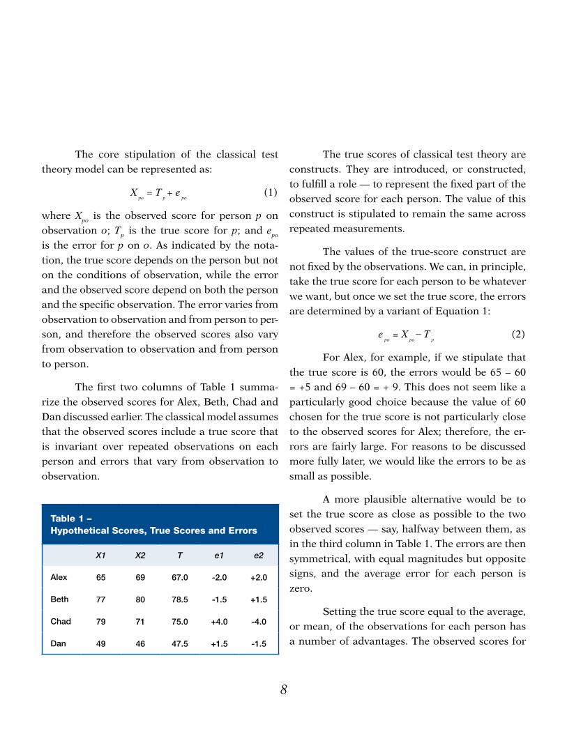
The first two columns of Table 1 summa-rize the observed scores for Alex, Beth, Chad and Dan discussed earlier. The classical model assumes that the observed scores include a true score that is invariant over repeated observations on each person and errors that vary from observation to observation.

Table 1 – Hypothetical Scores, True Scores and Errors

X1 X2 T e1 e2

Alex 65 69 67.0 -2.0 +2.0

Beth 77 80 78.5 -1.5 +1.5

Chad 79 71 75.0 +4.0 -4.0

Dan 49 46 47.5 +1.5 -1.5

The true scores of classical test theory are constructs. They are introduced, or constructed, to fulfill a role — to represent the fixed part of the observed score for each person. The value of this construct is stipulated to remain the same across repeated measurements.

The values of the true-score construct are not fixed by the observations. We can, in principle, take the true score for each person to be whatever we want, but once we set the true score, the errors are determined by a variant of Equation 1:

e po = X

po _ T

p (2)

For Alex, for example, if we stipulate that the true score is 60, the errors would be 65 – 60 = +5 and 69 – 60 = + 9. This does not seem like a particularly good choice because the value of 60 chosen for the true score is not particularly close to the observed scores for Alex; therefore, the er-rors are fairly large. For reasons to be discussed more fully later, we would like the errors to be as small as possible.

A more plausible alternative would be to set the true score as close as possible to the two observed scores — say, halfway between them, as in the third column in Table 1. The errors are then symmetrical, with equal magnitudes but opposite signs, and the average error for each person is zero.

Setting the true score equal to the average, or mean, of the observations for each person has a number of advantages. The observed scores for

8 9

each person are then clustered around the true score for the person, and the average value of the errors for the person is 0. This option also has sev-eral technical advantages.2

However, as stated, this option has a serious disadvantage. If we add another measurement for each of the four people, each person’s true score — defined as the average of their observed scores — is likely to change. However, the true score is not supposed to change, and it is especially not supposed to change just because we make another observation.

We can get around this problem by defin-ing the true score for each person as the expected value over all possible observations for that person — that is, as the average over a potentially infi-nite set of possible observed scores. This makes the true score an abstract quantity that cannot be observed directly, only estimated — but it makes for an invariant true score. The observed score for the person (based on a finite sample of observa-tions) can be employed as our best estimate of the true score.3 The observed scores that are treated as estimates of the true scores can change if we add additional observations (e.g., average over a larger sample of tasks or raters), but the true score for each person does not change.

Taking this approach, it is possible to stipu-late that the construct represented by the true score is fixed for each person, but to account for the fact that repeated measurements on a person generally yield different values by assigning the observed variability to random errors of measurement. The errors of measurement are not mistakes. I am assuming that the measurement procedure was implemented correctly, and the results were recorded as they occurred. The errors of measure-ment don’t exist in the data until we introduce them, but once introduced, they play a crucial role. They make it possible to describe phenom-ena in terms of general constructs, without be-ing immediately contradicted by the variability in observed scores.

sTaNdard errors aNd reliabiliTy CoeffiCieNTs

Estimating errors and true scores is nec-essarily a bit tricky, because neither true scores nor errors are directly observable. They are both constructs in the basic sense that we create them to serve our purposes.

In cases where it is possible to measure the same attribute of a person repeatedly without altering the value of the attribute for the person (e.g., measuring a person’s weight using a scale),

2 In particular, by choosing the average of the observed scores as the true score, we make the average of the squared values of the error as small as it can be, given the observed scores. As indicated later, the average squared error, or the error variance, is one commonly used index for the typical magnitude of the errors.

3 A person’s true score will generally not correspond to a possible observed score. The true score is a construct that we can imagine, talk about and estimate, but we cannot observe it directly. We define it, or construct it, as the expected value over all possible observed scores, because this choice is conceptually useful.

10 11

we can get a good estimate of the person’s true score by repeating the measurement a number of times (using different scales) and taking the average of the observed scores. The resulting average observed score is not equal to the true score, which is defined as the expected value (or average) over an infinite number of replications, but statistical sampling theory tells us that this average observed score can provide a pretty good estimate of the true score, with the precision of this estimate getting better as the number of observed scores over which the average is taken increases.

Given this estimate of the true score, we can estimate the error in any of the observed scores by subtracting the estimated true score from the observed score. Since the average value of the observed scores over the long term (i.e., over an infinite number of replications) is equal to the true score, the average value of the errors over the long term has to be zero, with about half of the errors being positive and half negative.

These errors are viewed as random fluctuations, or noise, and therefore the magnitude of any particular error is not of great interest in itself. Furthermore, since we can’t estimate the error in an observation until we have a good estimate of the true score, the estimated error for any particular observation is not helpful in estimating the true score.

Nevertheless, we would like to have some indication of the typical magnitude of the error as an indication of how good our estimate of the true score is. If the variability in the observed scores

around their mean observed score for a person is large, at least some of the errors of measurement in the observed scores have to be large, and any given observed score does not provide a good estimate of the true score for the person. If the variability around the mean is small, we have evidence to indicate that the random errors are not very large and that any observed score provides a good estimate of the true score.

The standard deviation is an index repre-senting the spread in a set of scores. If the scores are clustered tightly around their average value, the standard deviation will be small, and if the scores are spread out, the standard deviation will be large. With several separate observed scores for a person (e.g., scores obtained on different occa-sions or on different sets of tasks), the standard deviation of the observed scores for the person can be used to estimate the “typical” value of the error for the observed scores on the person, and this statistical index is referred to as the standard error of measurement, or the standard error, for the observed scores. If a person’s scores are clustered tightly around the person’s average score, the stan-dard error of measurement will be small, but if the person’s scores are spread out, the errors must be large and the standard error of measurement will be large.

This more or less direct estimation of the standard error of measurement works well if it is possible to obtain a fairly large number of independent observations on the same person.This approach has been used extensively in evaluating physical measurements, where the

10 11

act of measurement does not change the object, and the object (especially if inanimate) does not mind being measured. Things are different in the social sciences and in education; people tend to be less tolerant of being measured repeatedly, and they tend to change over repeated measurements, because of practice and learning, boredom, fatigue and so on. We have therefore developed a range of statistical models for estimating standard errors of measurement without having a large number of separate observed scores for each person.

For many of these alternative approaches (e.g., those involving reliability coefficients), we get two independent measurements on a large number of persons, and we use all of this data to estimate the average standard error of mea-surement for the persons. Even though people generally do not like taking tests, it is often possi-ble to get two separate measurements of the same kind on a large number of people (e.g., by having them take two different forms of the same test, or by having them take the same test on two occa-sions, or by generating separate scores from two halves of the test). We try to design these reliability studies so that the first testing will not have much, if any, impact on the results of the second testing.

Once we have two more-or-less indepen-dent measures of the same attribute using the

same measurement procedure, we can estimate a reliability coefficient for the test.4 If the two scores for each person are relatively close to each other (i.e., the within-person differences are small compared to the between-person differences), the reliability coefficient will be close to 1.0, its maxi-mum possible value. If the two scores for each person tend to be very different, the reliability coefficient will be close to 0.0. Using the basic assumptions of classical test theory, it is possible to demonstrate that the reliability coefficient is directly related to the proportion of the observed-score variability that is attributable to true-score variability, and then to derive an estimate of the average standard error of measurement for the measurement pro-cedure in the population. So, with only two scores for each person, we can get a fairly good estimate for the typical standard error of measurement for the people taking the test. These procedures do not provide separate estimates of each person’s standard error, but they do provide us with a general sense of how large the errors tend to be.

Standard errors can serve many purposes, but their main use is to provide an indication of how big the errors of measurement are likely to be, thereby providing an indication of how much confidence we can have in our estimate of the true value of the variable. In this vein, the observed score

4 In classical test theory, the reliability coefficient is typically estimated by computing the correlation over persons between the two sets of scores. Correlations are statistical indices designed to reflect the degree to which the relationship between the two sets of scores is linear. Cor-relation coefficients can have values between -1 and +1, but in the context of reliability studies in which the two measures (e.g., the same test given on two occasions or two forms of the same test) are very similar, correlations tend to have values between 0 and +1, with a correlation of +1 indicating a perfect linear relationship, and a correlation of 0 indicating no systematic relationship. In addition, in reliability studies, the two sets of scores are likely to have similar average scores and standard deviations, and as a result, a high reliability will indicate that the two scores for each person will tend to have similar values.

12 13

for each person can be reported with a confidence interval. Assuming that the test yields reliable results, the observed score is likely to be close to the true score, but it will not generally equal the true score. Using statistical sampling theory and the estimated standard errors, it is possible to construct a confidence interval around each score, such that the interval has some fixed probability of including the true score. For example, 95% confidence intervals would be expected to include the corresponding true score about 95% of the time. If the standard errors are relatively small, the confidence intervals will be relatively narrow, and our conclusions about the true score for each person can be relatively precise. So, we generally want the standard errors to be as small as possible.

raNdoM aNd sysTeMaTiC errors

The errors in classical test theory are essen-tially unpredictable fluctuations, or random noise. By definition, they are expected to have a mean of 0 and to be uncorrelated with each other and with all other variables. I will refer to such errors as random errors.

In contrast, systematic errors are constant across some set of scores (e.g., all scores for a particular person or occasion or test form) and are therefore potentially predictable. The classic

example of a systematic error is a miscalibrated bathroom scale — say, one that weighs 2 pounds too heavy. These systematic calibration errors do not have a mean of zero, but rather always have a value of +2, and therefore have a mean of +2. Random errors tend to cancel out in the long run. Systematic errors do not generally cancel out over the long run.

In some ways, random errors are easier to deal with and less serious than systematic errors, because random errors are generally easy to de-tect and estimate, and as discussed below, they can usually be controlled to some extent. As discussed earlier, they can be estimated by obtaining repeat-ed observations on persons and examining the variability in these observations for each person, or by getting two measurements on each person and estimating a reliability coefficient, and thence the average standard error of measurement. Since random errors tend to cancel out, we can generally decrease their magnitude by averaging over more observations and, in principle, we can make the standard error as small as we want by making the sample of observations large enough.5 Of course, the rub here is that additional observations gener-ally involve additional time and additional costs, and therefore adding enough observations to get the error down to where we might want it may not be practical.

5 The random fluctuations associated with errors of measurement tend to cancel out if we average over several observed scores (or over several observations within a test) to get a combined observed-score estimate of the true score. Statistical sampling theory indicates that the stan-dard error of measurement for the average over a sample of scores will be given by the standard error for a single score divided by the square root of the number of scores used to compute the average. So, as the number of independent observed scores included in the estimate of the true score increases, the standard error for the estimate gradually decreases, and the estimate of the true score gets more precise.

12 13

In some cases, systematic errors are easier to deal with than random errors. If we know what the systematic errors are (e.g., that the scale weighs 2 pounds too heavy), we can simply correct for the difference (i.e., subtract 2 pounds from the observed weight). This is essentially what is done when we calibrate an instrument: We ad-just the scale to eliminate any systematic errors that are detected. In this vein, equating models are used to correct for differences in the statisti-cal properties of standardized test forms (Angoff, 1971, 1987; Holland & Dorans, 2006; Kolen & Brennan, 2004, Livingston, 2004, von Davier, Hol-land, & Thayer, 2004).

However, in other cases, we may have rea-son to suspect that a systematic error exists, but not know its magnitude, or even its direction, and in these cases, we cannot remove it by adjusting the scores. If systematic errors cannot be removed, they tend to be more troublesome than random er-rors of the same magnitude, because they do not cancel out in the long run.

CoNTrolliNg raNdoM errors of MeasureMeNT

Sources of random errors can be controlled in two ways. First, the errors can be controlled to some extent by standardizing the measurement procedures. For example, the criteria used to rate performances can be specified in some detail, and the raters can be trained to use these procedures in a consistent and systematic way, thus reducing the random variation in scores associated with differences among raters. Similarly, the tasks

to be performed and the testing conditions can be standardized, so that extraneous factors that might have an impact on the performances are eliminated, or at least minimized. For example, if we find that there is a lot of variability in performance over tasks, we can consistently use the same kind of task, and in some cases, we can assign the same tasks (e.g., same questions) to everyone.

Standardization does have some limitations; in particular, it can introduce systematic errors (by fixing conditions of observation) as it reduces the random error. For example, if some students tend to do better on some kinds of tasks than on other kinds of tasks in the same content area (e.g., objective items vs. essays), standardizing the measurement procedure to one kind of task (e.g., objective items or essays) may give some students an advantage (positive systematic error) or a disadvantage (negative systematic error). As in many aspects of testing, we have a tradeoff. If we can get a large reduction in random error with the possibility of some small added systematic error, standardization is likely to be a good option. Standardization tends to play a large role in developing measurement procedures that yield precise results.

The second way to control random errors is to increase the number of observations that are sampled for each person. If we form a score by averaging over a sample of observations (e.g., responses to 100 multiple-choice questions, or performances on three occasions), the standard error in this mean score will be equal to the standard

14 15

error for a single observation divided by the square root of the number of observations. So it is generally a great advantage in controlling random errors to have a large sample of observations. The systematic relationship between the standard error and the number of observations is a major reason for the relatively high reliabilities and the relatively small standard errors of measurement associated with objective test formats (e.g., multiple choice, short answer), in which it is relatively easy to administer a large number of questions in a few hours. For performance tests or essay tests, it typically takes much longer to administer each task; therefore, the number of independently scored tasks is necessarily limited by the time constraints.

CoNTrolliNg sysTeMaTiC errors

It may be possible to correct for some sys-tematic errors by identifying the source of the error and eliminating, or at least minimizing it. In some cases, this is easy to do. For example, if a test with a fixed time limit starts late, it can be allowed to run late so that the students have the specified time to complete the test.

In other cases, the problem may be diffi-cult to fix. The argument for accommodations on standardized tests for students with disabilities is essentially an argument for removing a source of systematic error. The student with a disability is seen as being at a disadvantage in taking the test

because of the disability. For example, students with visual disabilities that slow their reading would be at a serious disadvantage on a timed test, and therefore their scores would be lower (a nega-tive systematic error) than the scores would be if the students did not have the visual disabilities. To correct for this source of error, a student could be given extra time to complete the examination. However, such disabilities tend to vary in severity, and therefore, it is hard to determine how much extra time to give each student in order to correct for the impact of the disability without overcor-recting.

In cases where it is not possible to physi-cally remove the source of systematic error or to make adjustments that correct for its effect, it may be possible to correct for the systematic error statistically. In standardized testing programs, different forms of the test are made as simi-lar as possible in content and difficulty, but the specific items are necessarily different (for security reasons), and therefore, there will be some differ-ences in difficulty. As a result of these differences in difficulty, the students taking the easier forms would tend to have an advantage, and the students taking the harder forms would tend to suffer a disadvantage, if nothing were done to correct for these differences. In practice, equating models are used to adjust, or equate, the score scales for the different forms to make them more or less equiva-lent (Angoff, 1971; Holland & Dorans, 2006).

14 15

MulTiple sourCes of error

Classical test theory assumes that we have a single, undifferentiated source of random error. In many cases, it is possible to identify different kinds of conditions over which observed scores might vary. For example, if we are considering a general attribute of persons (e.g., literacy in some language), we might expect the attribute to be rea-sonably stable across time, across social and phys-ical contexts, across language tasks, across raters (or observers), and so on. The actual observations are likely to vary along all of these dimensions, but the observed variability may be more dramatic over some dimensions than over others. For exam-ple, in a reading test, a person might handle some texts (those covering familiar content) better than other texts (those involving unfamiliar content and vocabulary), but show relatively consistent performance over contexts or raters.

To account for different possible sources of error in a measurement procedure, Cronbach and his associates (Cronbach, Gleser, Nanda, & Rajaratnam, 1972) introduced a theory of errors, called generalizability theory or G theory, that allows for multiple sources of error. G theory extends classical test theory in several directions and, in particular, it employs sophisticated statistical models to provide estimates of the variability (variance components) associated with different sources of measurement error. G theory allows for the possibility that the attribute to be measured may be stipulated to be invariant along several dimensions (facets in G theory). Within G theory,

the magnitudes of different sources of error can be estimated and combined (linearly) into a single overall standard error. This is not the place to discuss the details of this theory (see Brennan, 2001, for a good introduction), but I do want to make two points about how the random errors of measurement combine to form a single overall standard error of measurement.

First, combining different sources of error into a single estimate of error can be complicated. I will focus on the simple case of combining two random errors, e1 and e2. As discussed earlier, random errors are evaluated in terms of their standard deviations, or standard errors (SEs). As it happens, SEs are not additive, but the squares of the SEs (i.e., error variances) are additive. To get the total SE for two random errors, we square their SEs, add them together, and take the square root of this sum:

SE = √ (SE1)2 + (SE2)2.

If the standard errors are the same — say, SE1 = 1 and SE2 = 1 — the total standard error would be:

SE = √ (1)2 + (1)2 = √2 = 1.41.

The addition of a second error of the same size to the first error increases the overall standard error by 41%.

Second, if the two errors being combined are very different in magnitude, it turns out that the smaller error has very little impact. For example, if SE1 = 5 and SE2 = 1, the total standard error is:

SE = √ (5)2 + (1)2 = √26 = 5.10.

16 17

The second error, which is one-fifth (or 20%) the size of the first error, increases the overall stan-dard error by about 2%. Pushing this a bit further, if SE1 = 10 and SE2 = 1, the overall standard error is given by:

SE = √ (10)2 + (1)2 = √101 = 10.05.

In this case, the second error, which is one-tenth (or 10%) the size of the first error, increases the overall error by only about a half of 1%. The point is that with multiple sources of random er-ror, the larger errors have a disproportionate im-pact on the overall error, and it is the larger er-rors that need to be controlled. Smaller errors (i.e., those that are one-fifth the size of the larger errors or less) generally can be ignored.

error/ToleraNCe

As noted earlier, smaller standard errors are generally better than larger standard errors, and therefore, a lot of effort is devoted to controlling various sources of error by standardizing the measurement procedures and by identifying and controlling the most serious sources of error. However, many of the strategies for controlling errors of measurement (e.g., increasing the number of observations) require a lot of time, effort and expense, and therefore it is desirable to have criteria for deciding when the errors of measurement are effectively under control, or small enough.

In norm-referenced contexts, where the goal is to differentiate among the different levels

of true scores for the persons in some population, the magnitudes of the errors are evaluated rela-tive to the magnitudes of the true-score variability in the population. The index used to evaluate the magnitude of the errors relative to the magnitudes of the true-score variability for norm-referenced interpretations is the reliability coefficient (or generalizability coefficient). If the standard error of measurement is much larger than the standard deviation of the true scores in the population of interest, the reliability will be close to zero. If the standard error is much smaller than the standard deviation of the true scores, the reliability will be close to one. If the standard error is about the same as the standard deviation of the true scores, the reliability will be about 0.5. Generalizability coefficients typically follow the same pattern.

In the norm-referenced context, magnitudes of the differences between true scores define the tolerance for error. More generally, scores can be said to be precise enough if their standard errors are small compared to some reasonable tolerance for error in the situation under consideration (Kane, 1996). For example, in a licensure or certification context in which the goal is to determine whether each candidate’s true score is above some fixed cut score (or passing score), the tolerance for error might be defined by the magnitude of the difference between a person’s true score on the test and the cut score.

Basically, the criteria for determining whether the errors are small enough are defined in terms of the requirements of the particular interpretations and decisions that are to be based

16 17

on the test scores. If the errors are large enough that they distort the proposed interpretation of the scores or undermine the effectiveness of the decision procedures based on the scores, they constitute a serious problem, and if they do not interfere with the interpretations and decisions,

they are not very serious. When asked how long a man’s legs should be, Abraham Lincoln is reported to have said that they should be long enough to reach the floor; the errors should be small enough not to cause misinterpretations or misclassifications.

18 19

s indicated earlier, the conceptualization of our constructs has a major impact on what gets counted as error, and therefore, on the over-all magnitude of the standard error. Conversely, the magnitudes of various sources of error can have an impact on how we choose to define our constructs. If a very general interpretation for the construct, involving generalization over a very large domain of observations with many di-mensions (or facets), leads to unacceptably large errors, we may choose to narrow the interpretation.

In testing, each set of observations (re-sponses to test tasks) for a person is evaluated against some criteria (i.e., a scoring rule), yield-ing an observed score for the person, and the ob-served score is typically interpreted as an estimate of the expected score over a domain of possible observations associated with the construct. The interpretation depends on the specification of the domain, which may be defined broadly or narrowly. Typically, even the more narrowly defined domains include many different tasks, many different scorers, many different contexts and possibly many different occasions. The constructs so defined represent dispositions, or tendencies, to perform in certain ways over samples of tasks, scorers, situa-tions and occasions drawn from the domain.

The inference from a particular observed score, based on a sample of observations to a con-clusion about a general disposition, is an inductive inference from the sample to the domain of ob-servations from which the sample is drawn. Such inductive inferences always involve risk, or uncer-tainty, and we have to decide how much risk we

want to take and how much uncertainty we are willing to tolerate.

In generalizing over certain dimensions (e.g., tasks, occasions, contexts), we are purposely simplifying our model of reality to make it more amenable to concise description and analysis. In-stead of interpreting performance task by task, rater by rater, occasion by occasion, and context by context, we make general statements about overall performance across tasks, occasions and/or contexts. For example, instead of interpreting a person’s score on a reading test as a report of the person’s performance on a specific set of tasks (answering questions about certain short read-ing passages) on a particular day, in a particular classroom, we interpret the score as a measure of the person’s reading ability, or their level of liter-acy. This construct — reading ability — is defined in terms of expected performance over a variety of tasks, over an extended period of time, over a range of contexts, etc. Reading ability is a broadly defined disposition.

These dispositional constructs are, in a sense, mini-theories. Once the numerical value of the construct is estimated on some scale, this estimate can be used to predict how the student might perform on a different set of observations from the domain. A dispositional interpretation is much richer than a simple report of the observed score based on the observed performances. It is generally more useful to be able to draw conclu-sions about a student’s reading ability, conceived broadly, than to simply report the results of par-ticular observations.

A

the role of errors In defInIng VarIables/constructs

18 19

The richer interpretation inherent in dis-positional constructs rests on certain law-like assumptions, invariance assumptions, which claim that a person’s performance, and therefore his or her test scores, would not vary much over sam-ples of observations from the domain defining the disposition. As indicated earlier, the invariance assumptions hold by definition for the construct. By taking the construct to be the expected value (or average) over a domain of possible observations, we ensure that its value is not tied to any particu-lar sample of observations from the domain.

However, the observed scores based on samples of observations from the domain can cer-tainly vary from sample to sample, and the extent to which these observed scores satisfy the invari-ance assumptions is an empirical question, which is answered by evaluating how much variability is seen in a person’s observed scores across differ-ent samples from the domain. The world is almost always more complicated than our conceptual frameworks, and as a result, at best, the invari-ance assumptions hold only approximately for the observed scores. The extent to which the observed scores are invariant over samples from the domain can be determined by comparing scores based on different samples of tasks (e.g., in generalizability or reliability studies).

The choice about how widely to generalize conclusions based on test scores involves a decision about how to define the attribute being measured and how to talk about values of the attribute. If we assume invariance over some conditions of observation (e.g., occasions), we do

not have to mention those conditions in reporting the results, but if we do not intend to generalize over a condition of observation (e.g., time), we should mention it explicitly or implicitly in discussing the results. We can talk about measures of trait variables (e.g., height, aptitude), which are assumed invariant over extended periods of time, without specifying a particular occasion or situation; in fact, it would generally seem odd to specify a particular occasion or situation for a trait variable (e.g., to say that John’s aptitude was low at lunch yesterday). However, when we talk about state variables, which are not assumed to be invariant over occasions, it would generally be appropriate to specify a particular occasion or situation (e.g., John was in a good mood at lunch yesterday).

If the construct interpretation assumes invariance over a number of dimensions, the total standard error will involve the joint contribution of the errors associated with the different kinds of conditions of observation (e.g., tasks, occasions, raters, contexts) that are included in the domain. If we interpret a score in terms of a construct that is assumed to be invariant over a dimension, then variability in observed scores over that dimension is taken to be error, but if we don’t build invariance over a dimension into the construct definition, then variability over that dimension is simply variability over the dimension.

As indicated in the last section, it is possible to reduce errors of measurement by improving procedures (e.g., better training for raters) and by sampling the domain more thoroughly, particularly

20 21

by employing larger samples from the facets that contribute most to the overall standard error. However, all else being equal, the more broadly the construct is defined, the more error components will be included and the larger the overall error will be, and larger errors lead to more tentative and less dependable inferences (i.e., estimates with broad confidence intervals) about the true value of the dispositional construct. Therefore, we prefer that the overall standard error be relatively small.

This choice of how broadly to define a dispositional construct involves a tradeoff between the generality of the construct and the accuracy with which we can estimate it. A broadly defined construct is potentially more useful than a narrowly defined construct, but in general, the estimates of broadly defined constructs are more error prone than the estimates of narrowly defined constructs.

20 21

t is very appealing to use scores on standard-ized tests as the basis for high-stakes decisions. These data can be relatively easy and cheap to col-lect and to interpret. A high score is better than a low score, and if we have a cut score specifying the criterion for adequacy, it is easy to decide whether the performance is adequate: If the score is at or above the cut score, the performance is adequate. In evaluating a school, it is certainly more conve-nient to consider a single average test score or the percentage of students above some cut score than to have a team of qualified examiners conduct a site visit and report their findings in an extended narrative.

Standardized, objective measurement procedures offer the promise of accurate and fair assessment as the basis for accurate and fair decisions, and in most cases, it is arguable that they deliver on this promise. They tend to have technical properties that are better than the alternatives, such as interviews, GPAs and other data in academic records, and evaluations of student portfolios. In particular, it is generally possible to estimate the random errors and at least some of the systematic errors associated with standardized tests, and therefore, to control for these errors to some extent. This kind of error analysis and control is not generally possible for unstandardized procedures because, by definition, they keep changing in various ways.

But convenience, economy and technical quality are not necessarily the main advantages associated with the use of standardized test scores to make high-stakes decisions. Rather, a good case

can be made that it is the “objectivity” of objective tests that accounts for much of their appeal to decision makers (Porter, 1995).

Of particular importance in high-stakes decision making, the use of objective procedures makes it more likely that the decisions will be free of overt bias. In highly standardized testing proce-dures (e.g., multiple-choice tests), the assessment procedures are essentially the same for everyone, the scoring is automatic, and the analyses and reporting are done by staff who never see or inter-act with the test takers. As a result, standardized assessment procedures can promote both fairness and the appearance of fairness. Theodore Porter (1995) suggested that our trust in objective quan-titative measures has its roots in a rejection of inequality in favor of democracy:

This is why a faith in objectivity tends to be associated with political de-mocracy, or at least with systems in which bureaucratic actors are highly vulnerable to outsiders.… Scientific objectivity thus provides an answer to a moral demand for impartiality and fairness. Quantification is a way of making decisions without seeming to decide. (Porter, 1995, p. 8)

The same general regard for consistency in the treatment of individuals is enshrined in our legal system as procedural due process.

At their best, test-based decision pro-cedures tend to promote both fairness and the appearance of fairness, but — not surprisingly —

I

errors of measurement In PublIc PolIcy

22 23

their effectiveness can be diminished by errors of measurement. In this section, I will examine some of the roles played by errors of measurement when tests are used to implement public policy.

CerTifiCaTioN TesTiNg

A major high-stakes application of testing in our society is in certifying qualifications for some activity or profession. Licensure examina-tions, ranging from the test required for a driver’s license to the multi-day examinations required for licensure in a profession (e.g., medicine, law) have important consequences for the applicants tak-ing the test, and for the public, who rely on these programs to provide some assurance of a licensed person’s basic competence in the relevant activity (Shimberg, 1981).

In licensure testing and in many other high-stakes testing contexts, errors of measurement play a critical role in test development and in evaluat-ing the testing program. The standard errors also may play a role in defining the score scales and in setting the passing scores. However, the standard error for an individual candidate’s score is gener-ally ignored in making a decision about licensure for the candidate. Errors of measurement are not explicitly included in the decision rules used to award or withhold a license. Once the testing procedures are developed and the passing score is specified, the decisions are more or less automat-ic. If a candidate’s observed score is at or above the passing score, the candidate passes; otherwise, the candidate fails.

In a sense, we have two distinct models or views of test scores operating at different stages in the operation. In developing the testing program, measurement models generally play a major role, and the test scores are viewed as fallible estimates of constructs or true scores. In using the resulting test score to decide whether to certify a particular candidate, the candidate’s score is generally treat-ed as a factual summary of the candidate’s perfor-mance on a particular test date, and errors of mea-surement are not considered. An assertion that the candidate might have done better or worse on a different day, or at a different test site, or on a dif-ferent form of the test, would be discounted as an irrelevant, contrary-to-fact conjecture.

Candidates for professional licensure (or for a driver’s license) typically “sit for an exam,” and candidates with scores at or above the pass-ing score pass, and those with scores below the passing score fail. It is a simple rule, and is based, as they say, on a bright line. If a candidate has a score near the passing score, a measurement theo-rist might be tempted to suggest that the issue is in doubt because, given the potential error of mea-surement, a reasonable confidence interval for the candidate’s true score (i.e., the candidate’s typical level of performance) includes the passing score.

In such circumstances, we could suspend judgment about candidates with scores just above or below the passing score and collect more in-formation in order to get a better estimate of the candidate’s true score, defined as their expected (or average) score over all possible replications of the measurement procedure (e.g., by employing

22 23

two-stage testing or some other kind of adaptive testing). However, most licensure and certification programs employ a single one-stage design: candi-dates with observed scores at or above the passing score pass, and candidates with observed scores below the passing score fail.

In most high-stakes testing programs, esti-mates of different kinds of random and systematic error are used to evaluate the technical character-istics of the testing procedure and, where possible, to improve the process by identifying aspects of the tests or the procedures that can be improved. For example, if the test scores are found to be un-reliable, the testing procedures may be tightened, or the number of responses that are sampled may be increased. If it is found that the grading of re-sponses for essays or performance tasks is not very consistent, the graders might be given more explicit grading guidelines, or more training, or more careful monitoring and retraining.

However, in making decisions about indi-vidual candidates, a more matter-of-fact attitude is adopted, and the assumption that the observed score is a fallible measure of some true score, which is at the core of test theory, is not allowed to soften or blur the bright line. In most legal and administrative contexts, the focus is on what oc-curred, not on what might have occurred in a hy-pothetical replication of the testing procedure. So, if there were no mistakes made in either adminis-tering or scoring a test, there is, in this sense, no error. This is not the standard psychometric view, but it is a very reasonable point of view. As noted

earlier, observations are what they are. Concerns about what the results would be if the testing pro-cedure were replicated (once or an infinite number of times) are what are called contrary-to-fact con-ditionals, and in implementing the decision rules in most high-stakes testing contexts, contrary-to-fact conditionals are not considered.

No Child lefT behiNd

Under the No Child Left Behind (NCLB) Act (2002), student scores on state tests in core content areas (basically, reading and mathematics) are ad-ministered each year to essentially all students in the states in grades 3 to 8, and in science at some grade levels. The results are to be used to evalu-ate schools and, in particular, to hold the schools accountable for their students’ achievement. This use of test scores to promote school accountabil-ity and student achievement is relatively new to educational measurement. We have evolved from a view of tests as measurement instruments (Cure-ton, 1951), to a recognition that testing programs can have an impact on educational outcomes (Crooks, 1988; Moss, 1998), and now to the use of test scores as engines of educational accountabil-ity (NCLB).

Each state specifies the required content in the core subjects for its students and develops tests based on these specifications. The state tests focus on the core content areas of mathemat-ics and reading, and even in these areas they do not cover everything in the state content outlines. So, as measures of school effectiveness, the state

24 25

tests are limited. At best, they measure student achievement on a subset of the desired outcomes of schooling.

Under NCLB, student scores on the state tests are transformed to achievement levels, developed to reflect four different levels of performance (e.g., below basic, basic, proficient, and advanced). The four achievement levels are defined by three cut scores on the score scale for the test (for the basic, proficient and advanced levels). All students with scores below the cut score for the basic level are classified as being below basic, students with scores between the basic cut score and the proficient cut score are considered to be at the basic level, and so on. The goal is to define state standards for performance in the core content areas and to encourage all students to reach a predefined level of achievement (i.e., the proficient level). The reduction of the test scores to a few achievement levels involves some loss of information, but is intended to make the results more easily interpretable.

The achievement-level classifications are aggregated over students in each school and each grade to yield the percentage of students at each achievement level in each grade within the school (and within various subgroups at each grade level), and the schools are evaluated in terms of the percentages of their students at or above the proficient level. Schools that fail to achieve certain increases in the percentages of students at or above the proficient level (i.e., that fail to make adequate yearly progress) are labeled as needing improvement. If a school fails to meet the targets

for improvement over several years, it is subject to sanctions.

A distinguishing feature of test-based accountability programs is their focus on achieving certain goals, and not on the measurement of any particular attributes. This is particularly true of the NCLB legislation. The provisions of this act include mandates on when testing is to occur (grades 3 through 8), which students are tested (requirements on participation rates for various groups), and consequences for schools that fail to achieve adequate yearly progress, but the act defers to the individual states’ standards on the content and format of the tests and on the definition of the achievement levels (Linn, 1997).

The avowed purpose of the NCLB legislation is to promote accountability for schools and thereby to promote student learning. The rhetoric supporting the program is particularly emphatic about promoting the achievement of at-risk, low-performing students. These are the students most likely to be left behind and it is the mandate of the program that they not be left behind.

This focus on measurable outcomes and accountability has given rise to a need for accurate measurements of student outcomes. If we are going to hold a school accountable (and possibly impose serious sanctions) for failing to meet some benchmark (e.g., adequate yearly progress in the percentage of students achieving the proficient level, which is supposed to reach 100% by 2014), we need some dependable way of determining whether the benchmark has been reached, and

24 25

an appropriate theory of errors makes it possible to evaluate the dependability of the results of the testing program.

The NCLB accountability system is prone to a number of potential sources of systematic and random errors, which could undermine the effectiveness of the program. Some of the more significant systematic errors arise from the fact that the results are used to hold schools accountable for their students’ achievement, and the results (i.e., the percentages of students in each grade level and in each subgroup who are at or above the proficient level) are interpreted as indicators of the effectiveness of the school. Under this interpretation, any factor that influences the student outcomes that is not under the control of the school is a potential source of systematic error. To the extent that students come to school with different levels of preparation and have different opportunities to learn outside of school, some of the differences in student outcomes are not attributable to school effectiveness. As a result, any systematic differences among schools in the degree to which their students benefit from, or are hampered by, outside influences on learning (e.g., because of the location of the school and the populations served) would introduce systematic errors into the estimates of school effectiveness.

The accountability system itself may intro-duce a number of sources of systematic error into the indicators of school effectiveness by introduc-ing perverse incentives. As mentioned earlier, the state tests that are used to generate the scores on which the school-level indicators are based do not

cover all of the desired outcomes of education, and to the extent that some schools focus on the content that is tested, at the expense of nontested content, the percentages of students at or above the proficient level can be inflated. In addition, the school-level results will be skewed if some schools fail to test many low-scoring students; to address this issue, NCLB includes participation rules.

Less obviously, perhaps, the measures of school effectiveness used in NCLB tend to be subject to large random errors. The shift from individual student scores to school-based percentages at or above the proficient level shifts the focus from individual students to schools. In considering the standard errors associated with test scores for individual students, the common sources of error that are likely to be considered are the sampling of test tasks, occasions, contexts and, if the responses have to be evaluated by a rater, the sampling of raters. Each of these potential sources of error will generate some random error and may, in addition, introduce some systematic errors (e.g., some raters being more severe than others).

In developing standardized testing pro-grams, all of these common sources of error are likely to be controlled in some way. The variability associated with the sampling of test items can be controlled through careful item development, by basing scores on many items and, if appropriate, by employing statistical equating. The variability associated with occasions is addressed by giving the tests to all students at about the same time. The variability associated with contexts is ad-dressed by administering the tests to all students

26 27

in a fairly standard, neutral way. Rater variability is controlled by developing clear rating criteria and by training the raters to be consistent in their evaluations. It is not possible to eliminate any of these sources of error completely, but for stan-dardized testing programs, it is generally possible to control them reasonably well.

However, in using test scores to hold schools accountable, it is the overall performance of the students in the school (in particular, the percentages of students at each grade level, in each content area, and in various subgroups that achieve the proficient level on the state tests) that is the variable of interest. For this purpose, the variability in performance from one student to another has to be considered a source of error, and this source of error is likely to be large, both for the average scores for the students in various groups at various grade levels and for the percentages of students at or above the proficient level (Brennan, Yin, & Kane, 2003).

Standardized tests are not typically de-signed to control the variability across students, because the tests are designed to measure differ-ences in student achievement. In fact, traditional test development procedures are designed to maxi-mize the variability associated with student differ-ences, while minimizing the variability associated with the sampling of test tasks, occasions, contexts and raters (if appropriate).

It is obviously not feasible to control this source of error by controlling which students go to each school. Assuming that the goal is to evaluate

the educational effectiveness of the schools, it would, from an experimental-design point of view, be desirable to randomly assign students to schools, but this is clearly not practical. It is also probably not desirable from an educational or social point of view. So we are stuck with potentially large random and systematic errors in evaluating schools under the current NCLB model.

The value-added models that have been proposed as improvements on the current NCLB model are designed to statistically adjust for the differences in the student populations in differ-ent schools. These models hold some promise for controlling the main source of error in the current NCLB program, but the value-added models face some formidable technical problems.

Test scores can be blunt instruments for accountability purposes, and they are likely to be especially blunt if we don’t pay attention to controlling the larger sources of random and systematic errors.

errors, soCial CoNsequeNCes aNd ValidiTy

The consequences of test use have always been an important consideration in evaluating testing programs, but the emphasis has generally been on immediate consequences for the person taking the test or the institution using the test score to make a decision. For example, place-ment tests and admissions tests are evaluated in terms of how successful placed/admitted students are in their educational program. In general, de-cision procedures are evaluated in terms of their

26 27

outcomes and their consequences (i.e., positive and negative), and we have a long tradition of evaluating intended outcomes/consequences (e.g., in placement testing, admission and employment testing).

A major theme in Samuel Messick’s (1988, 1989, 1994, 1998) writings was the claim that the larger social consequences of testing programs have a role in evaluating (or validating) these programs. In part because this view ran counter to the traditional view of measurement as a neutral, objective, scientific enterprise, and partially because of the perceived difficulty in sorting out social consequences, the role of social consequences in evaluating testing programs has been a matter of some controversy (Linn, 1997; Popham, 1997; Shepard, 1997).

The Standards for Educational and Psy-chological Testing define validity as “the degree to which evidence and theory support the inter-pretation of test scores entailed by proposed uses of tests” (American Educational Research Asso-ciation, American Psychological Association, & National Council on Measurement in Education [AERA, APA, & NCME], 1999, p. 9). A proposed test-score interpretation or use is said to be valid if it can be shown to be plausible, using appropriate theory and evidence. A central concern in valida-tion is the potential impact of various sources of error, systematic and random. If any source of er-ror is found to be large enough to undermine the proposed interpretation or use, the interpretation/use is considered invalid.

It seems clear that social consequences should have some role in evaluating testing programs, if only in the negative sense that we expect all decision procedures to avoid serious negative consequences, but it is less clear what that role should be. In particular, there is some debate about whether social consequences should be considered under the heading of validity, or should be excluded from the criteria for evaluating the quality of testing program and relegated to a separate sphere of policy analysis (Popham, 1997).

Messick (1989) suggested that validation would include, “an appraisal of the social consequences of testing” (p. 88), but seemed to see negative consequences as counting against the validity of a testing program only if the negative consequences could be attributed to some source of error in the test:

… it is not that the adverse social con-sequences of test use render the use invalid but, rather, that adverse social consequences should not be attribut-able to any source of test invalidity such as construct-irrelevant variance. If the adverse social consequences are empirically traceable to sources of test invalidity, then the validity of the test use is jeopardized. If the social consequences cannot be so traced … then the validity of the test use is not overturned. Adverse social consequences associated with valid

28 29

test interpretation and use may impli-cate the attributes validly assessed, to be sure, as they function under the ex-isting social conditions of the applied setting, but they are not in themselves indicative of invalidity. (Messick, 1989, pp. 88-89)

The 1999 edition of the Standards (AERA, APA, & NCME, 1999) incorporated this view of the role of social consequences in validity: “Thus, evidence about consequences may be directly relevant to validity when it can be traced to a source of in-validity such as construct underrepresentation or construct-irrelevant components” (p. 16). It also stated, “Evidence about consequences that cannot be so traced — that in fact reflects valid differences in performance — is crucial in informing public decisions, but falls outside of the technical pur-view of validity” (p. 16).

This position seemed strange to me, because it seemed to say that adverse consequences could invalidate a proposed use of test scores, but only if the proposed interpretation/use had already been invalidated or, at least, could be invalidated in some other way. Although Messick was criticized for giving social consequences too much of a role in validity, in fact the role seemed so mild as to be almost nonexistent. It seemed that adverse consequences could only invalidate a test use if the proposed interpretation/use of the test scores were already invalid.

One way to resolve this paradox (i.e.,that consequences have an important role in validation,

but only if the test-score interpretation is invalid) is to treat the discovery of negative social consequences as an impetus to critically evaluate the assumptions built into the interpretation and use of the scores. For example, in the past, the perceived need for physical strength in the work of police officers and firefighters led to height and weight requirements for these jobs. The measures of height and weight were presumably valid as measures of height and weight, but their relationship to job performance was more questionable (Jackson, 1994). The fact that these requirements had adverse impact on protected groups (particularly women) led to a more critical evaluation of their assumed relationship to job performance, and because their relationship to job performance had not been demonstrated, they were rejected by the courts (Campion, 1983). The height and weight requirements were replaced by measures of the ability to perform activities (e.g., carrying an adult down a ladder) involved in the work requirements of firefighters and police (Jackson).

An alternative analysis of the role of social consequences in validation makes use of some of the points developed earlier about combining dif-ferent sources of error. Evaluations of validity do not yield a yes or no answer. Test scores always con-tain errors, both random and systematic. In this sense, interpretations/uses are never completely valid. In the example given above, the measures of height and weight were accepted for many years as rough indicators of strength, and in samples of reasonably fit applicants, height and weight would

28 29

probably be positively correlated with strength. However, height and weight are pretty rough in-dicators of strength; some short, slight people are more capable of performing physically demand-ing tasks than some taller, heavier people. These discrepancies constitute systematic errors in inter-preting height and weight as indicators of strength for individuals, but these systematic errors were not seen as major problems until they were found to have adverse impact on protected groups.

In comparisons between groups, the ran-dom errors tend to wash out because of the large sample sizes used to compute group means. Sys-tematic errors that are specific to individuals and not related to group membership also tend to av-erage out. However, systematic errors linked to group membership will not wash out of the group means. Because women tend to be shorter and lighter, on average, than men, the errors associated with using height and weight to estimate strength tended to exclude most women from getting jobs as police or firefighters.

Systematic errors that are small enough relative to the random errors that they can be ignored for individuals may have important consequences for groups. For example, suppose that we have a random error of 10 points on some scale, and a systematic error of 1 point. The random error is 10 times larger than the systematic error,

and therefore, in interpreting individual scores, the systematic error can be largely ignored. As noted earlier, a random error of 1 combined with a random error of 10 increases the overall error to about 10.05, an increase of half of 1%; combining a systematic error of 1 with a random error of 10 will have a similar effect, leading to an overall error of about 10.05. On the individual level, the systematic error has very little impact, and therefore, can be ignored at this level.

However, if the systematic error has a dif-ferential impact on the scores of different groups, we may arrive at a very different conclusion about group-level performance. If the systematic error produces a difference of 1 point between the aver-age scores for the two groups, this difference will be essentially independent of the sizes of the sam-ples from the two groups. However, the random errors in the group means will tend to wash out as the sample sizes for the two groups increase. At the group level, the systematic errors may be as large as or larger than the random error, and therefore, the relatively small systematic error that is inconsequential on the individual level may be quite consequential on the group level.6

Under this interpretation, the role of con-sequences proposed by Messick and the Standards does have teeth. Small systematic errors that are related to group membership may be negligible

6 The importance of these group differences in average scores can be magnified by the fact that in some cases, even modest differences in group means can lead to substantial difference in acceptance rates or pass rates, or percentages at specific achievement levels. For example, if the cut score is near the average score for a group, many individuals will have scores around the cut score, and even a small shift in the distribu-tions of scores (or in the cut score) can make a relatively large difference in the percentage below the cut score.

30 31

compared to the random errors and, therefore, be ignored in evaluating the validity of the test scores at the individual level. In estimating group means, however, the random errors (and some systematic errors) will tend to cancel out; therefore, system-atic errors that are related to group characteristics will have a large impact relative to the random er-rors. At the individual level, the random errors tend

to dominate, but at the group level, any systematic errors that are related to group membership tend to dominate and to be much more noticeable than they are at the individual level. So an evaluation of social consequences can add a major dimension to validation by identifying systematic errors that might otherwise go unnoticed.

30 31

eality is complicated, but our models of reality tend to be relatively simple, involving a few factors that are thought to have a substantial impact on the outcomes of interest. In order to avoid being overwhelmed by detail, we limit the number of variables to which we attend. In the so-cial sciences and education, we generally focus on variability across persons. Variability over some other dimensions (e.g., changes over time, differ-ences in task difficulty, the impact of context) also may be explicitly modeled, but it is hard to analyze variability over more than two or three dimen-sions at the same time. We smooth over the gaps between our simple models and a complex reality by introducing the concept of errors of measure-ment, and we relegate most potential sources of variability to that other category that we call error.

errors of MeasureMeNT aNd Their CoNTrol

Errors of measurement make it possible to interpret test scores in a fairly general way, but as is usually the case, there is no free lunch. The adoption of a theory of error forces us to add a penumbra of uncertainty in the form of standard errors to our estimates of the construct, and the more sources of variability that we relegate to er-ror, the larger the overall uncertainty. An increase in uncertainty is seen as an acceptable price for greater generality in the interpretation of test scores, as long as the range of uncertainty does not get too large — that is, as long as the errors are small enough that they do not interfere with

the interpretation or use of the test scores. If the errors are large compared to the differences of interest, they are too large. For traditional norm-referenced tests, the interpretation is focused on differences among persons, and therefore, if the errors are small compared to the variability in the true scores for persons, the errors are considered small enough.

More generally, for errors to play their intended role effectively, they have to be small compared to the score differences that determine the outcomes of the decisions to be made (e.g., for licensure examinations, the difference between a person’s score and the passing score). If the errors of measurement are large compared to the tolerance for error, they need to be reduced by controlling the largest sources of error.

In order to effectively control the over-all error, including the random and systematic components, it is particularly important to con-trol the larger sources of error. If a source of error (systematic or random) is small compared to the dominant sources of error for a measurement procedure (e.g., less than one-fifth of the larger error), it can generally be ignored. However, sys-tematic errors that are inconsequential at the in-dividual level because they are small compared to the random errors in student scores may have seri-ous consequences at the group level, particularly if they have disproportionate impact on racial/ ethnic groups (or other protected groups).

R

concludIng remarks

32 33

The role of errors iN defiNiNg Variables/CoNsTruCTs

We decide how we describe reality. By assigning the variability associated with certain dimensions (e.g., contexts) to errors of measurement, we implicitly adopt invariance assumptions, which claim that the student’s true score on the construct of interest (but not the observed scores) does not vary over these dimensions (e.g., contexts). The construct of interest is taken to be invariant over the dimension, and the observed variability associated with the dimension is taken to be random noise in the estimates of the construct.

We want our constructs to be general, and therefore we assume invariance over many dimensions; as a result, the observed scores involve many sources of error. At the cost of admitting some uncertainty, we gain generality in the inferences made from test scores. Instead of saying that a student got a high score on a certain multiple-choice geography test on a certain date in a certain class, and so on, we say that the student has high achievement in geography. The first statement is very specific, and assuming that no procedural mistakes were made in administering the test and scoring the results, it is essentially certain; the second statement is more general and useful, but it takes a lot of invariance assumptions for granted, and is therefore more uncertain. The invariance assumptions typically do not hold exactly, with discrepancies accounted for by the errors of measurement.

We can define our constructs narrowly in terms of the kinds of observations used to generate the observed scores (e.g., in terms of performance on questions about reading passages under certain conditions). Under this interpretation, we can be quite confident about the accuracy of our very limited conclusions. Alternately, we can define the construct more broadly (e.g., in terms of literacy, or reading ability). The more broadly defined constructs tend to be more useful, but they also involve more inferential risk and uncertainty.

errors of MeasureMeNT iN publiC poliCy

The use of test scores to make high-stakes decisions has many advantages. Standardized tests can often provide more accurate and precise assessments than alternative methods (e.g., inter-views, academic records, supervisor evaluations), but it is their objectivity that may be particularly appealing to decision makers.

Standardized procedures promote both fairness and the appearance of fairness. They can provide efficient and relatively accurate measures of variables that are relevant to the decision with-out relying on any subjective judgments. As noted earlier, they can help us to make high-stakes deci-sions “without seeming to decide” (Porter, 1995, p. 8).

However, policymakers tend to give short shrift to errors of measurement, systematic and random. This is not surprising because most policymakers do not know a lot about measure-ment theory or about errors of measurement,

32 33

and in many cases, the errors do not make much difference at the policy level. Most of the effort given to identifying, estimating and controlling errors of measurement occurs during test devel-opment, and assuming that the errors are not so large as to interfere with the intended interpreta-tion and use of the test scores, they do not need to be given much explicit attention at the policy level. The decisions are based on the actual per-formance of candidates, as reflected in their ob-served scores, without entertaining hypotheses about what the scores might have been under other circumstances.

In cases where the test results are used to hold institutions accountable, as in estimates of group means and under the NCLB legislation, the errors of measurement tend to be dominated by the variability in student scores within the institutions being evaluated. In classical test theory, the variability associated with differences across persons is taken as true-score variability, and tests are designed to maximize this variability. However, in estimating group means (e.g., in order to monitor changes in average scores over time, or to examine differences across racial/ethnic groups) variability across samples of students counts as error. In estimating the overall effectiveness of

schools under the NCLB program, the percentages of students in various groups achieving the proficient achievement level is the bottom line, and the random and systematic errors associated with student variability tend to be substantial and to constitute a major threat to the effectiveness of the accountability program.

More generally, in evaluating programs and policies, consequences play a major role, and in cases where testing programs have social consequences, it would be reasonable to evaluate the programs in terms of these social consequences. However, it also seems reasonable that negative social consequences count against the validity of test use only if the interpretation underlying the test use is already invalid. As indicated earlier, this paradox can be resolved by recognizing that systematic errors that are negligible at the individual level may be relatively large at the group level. A systematic error that is too small to invalidate a proposed interpretation at the individual level can invalidate a corresponding interpretation at the group level.

As Kyburg (1968, p. 140) pointed out, “er-ror is a delicate concept,” but analyzed carefully, it has a lot to tell us.

34 35

American Educational Research Association, American Psychological Association, & National Council on Measurement in Education. (1999). Standards for educational and psychological test-ing. Washington, DC: American Educational Research Association.

Angoff, W. (1971). Scales, norms, and equivalent scores. In R. L. Thorndike (Ed.), Educational mea-surement (2nd ed., pp. 508-600). Washington, DC: American Council on Education.

Angoff, W. (1987). Technical and practical issues in equating: A discussion of four papers. Applied Psychological Measurement, 11, 291-300.

Angoff, W. (1988). Validity: An evolving concept. In H. Wainer & H. Braun (Eds.), Test validity (pp. 9-13). Hillsdale, NJ: Lawrence Erlbaum.

Brennan, R. (2001). Generalizability theory. New York: Springer-Verlag.

Brennan, R., Yin, P., & Kane, M. (2003). Method-ology for examining the reliability of group mean difference scores. Journal of Educational Measure-ment, 40(3), 207-230.

Campion, M. (1983). Personnel selection for phys-ically demanding jobs: Review and recommenda-tions. Personnel Psychology, 36, 527-550.

Cronbach, L.J., Gleser, G.C., Nanda, H., & Raja-ratnam, N. (1972). The dependability of behavioral measurements: Theory of generalizability for scores and profiles. New York: Wiley.

Crooks, T.J. (1988). The impact of classroom evalu-ation practices on students. Review of Educational Research, 58, 438-481.

Cureton, E.E. (1951). Validity. In E.F. Lindquist (Ed.), Educational measurement. Washington, DC: American Council on Education.

Holland, P., & Dorans, N. (2006). Linking and equating. In R. Brennan (Ed.), Educational mea-surement (4th ed., pp. 187-220). Westport, CT: American Council on Education.

Jackson, A. S. (1994). Preemployment physical evaluation. Exercise and Sport Science Review, 22, 53-90.

Kane, M. T. (1996). The precision of measure-ments. Applied Measurement in Education, 9(4), 355-379.

Kolen, M.J., & Brennan, R.L. (2004). Test equating, scaling, and linking. New York: Springer.

Kyburg, H. (1968). Philosophy of science: A formal approach. New York: Macmillan.

Linn, R.L. (1997). Evaluating the validity of as-sessments: The consequences of use. Educational Measurement: Issues and Practice, 16(2), 14-16.

Livingston, S.A. (2004). Equating test scores (with-out IRT). Princeton, NJ: ETS.

Lord, F.M., & Novick, M.R. (1968). Statistical theo-ries of mental test scores. Reading, MA: Addison-Wesley.

references

34 35

Messick, S. (1988). The once and future issues of validity. Assessing the meaning and consequences of measurement. In H. Wainer & H. Braun (Eds.), Test validity (pp. 33-45). Hillsdale, NJ: Lawrence Erlbaum.

Messick, S. (1989). Validity. In R.L. Linn (Ed.), Ed-ucational measurement (3rd ed., pp. 13-103.) New York: American Council on Education.

Messick, S. (1994). The interplay of evidence and consequences in the validation of performance as-sessments. Educational Researcher, 23, 13-23.

Messick, S. (1998). Test validity: A matter of conse-quences. Social Indicators Research, 45, 35-44.

Moss, P. A. (1998). The role of consequences in va-lidity theory. Educational Measurement: Issues and Practice, 17(2), 6-12.

No Child Left Behind Act of 2001, 20 U.S.C. § 6301 et seq. (2002).

Popham, W.J. (1997). Consequential validity: Right concern — wrong concept. Educational Measure-ment: Issues and Practice, 16(2), 9-13.

Porter, T. (1995). Trust in numbers: The pursuit of objectivity in science and public life. Princeton, NJ: Princeton University Press.

Shepard, L.A. (1997). The centrality of test use and consequences for test validity. Educational Mea-surement: Issues and Practice, 16(2), 5-8, 13, 24.

Shimberg, B. (1981). Testing for licensure and cer-tification. American Psychologist, 36, 1138-1146.

von Davier, A.A., Holland, P.W., & Thayer, D.T. (2004). The kernel method of test equating. New York: Springer.

36

12615

About ETS

At nonprofit ETS, we advance quality and equity in education

for people worldwide by creating assessments based on rigorous

research. ETS serves individuals, educational institutions and

government agencies by providing customized solutions for

teacher certification, English-language learning, and elementary,

secondary and post-secondary education, as well as conducting

education research, analysis and policy studies. Founded in 1947,

ETS develops, administers and scores more than 50 million tests

annually — including the TOEFL® and TOEIC® tests, the GRE®

test and The Praxis Series™ assessments — in more than 180

countries, at over 9,000 locations worldwide.