error-detecting and error- correcting capabilities of a...

49

Error-Detecting and Error-

Correcting Capabilities of a Block

Code

50

Error-Detecting and Error-Correcting

Capabilities of a Block Code

If the minimum distance of a block code C is dmin, any

two distinct code vector of C differ in at least dmin places

A block code with minimum distance dmin is capable of

detecting all the error pattern of dmin – 1 or fewer errors

However, it cannot detect all the error pattern of dmin

errors because there exists at least one pair of code

vectors that differ in dmin places and there is an error

pattern of dmin errors that will carry one into the other

The random-error-detecting capability of a block code

with minimum distance dmin is dmin – 1

51



An (n, k) linear code is capable of detecting 2n – 2k error patterns of length n

Among the 2n – 1 possible nonzero error patterns, there are 2k – 1 error patterns that are identical to the 2k – 1 nonzero code words

If any of these 2k – 1 error patterns occurs, it alters the transmitted code word v into another code word w, thus w will be received and its syndrome is zero

There are 2k – 1 undetectable error patterns

If an error pattern is not identical to a nonzero code word, the received vector r will not be a code word and the syndrome will not be zero

52



These 2n – 2k error patterns are detectable error patterns

Let Al be the number of code vectors of weight i in C, the numbers

A0, A1,..., An are called the weight distribution of C

Let Pu(E) denote the probability of an undetected error

Since an undetected error occurs only when the error pattern is

identical to a nonzero code vector of C

where p is the transition probability of the BSC

If the minimum distance of C is dmin, then A1 to Admin – 1 are zero

1

( ) (1 )n

i n i

u i

i

P E A p p

53



Assume that a block code C with minimum distance dmin is used for

random-error correction. The minimum distance dmin is either odd

or even. Let t be a positive integer such that:

2t+1≤ dmin ≤2t+2

Fact 1: The code C is capable of correcting all the error patterns of t

or fewer errors.

Proof:

◦ Let v and r be the transmitted code vector and the received vector,

respectively. Let w be any other code vector in C.

d(v,r) + d(w,r) ≥ d(v,w)

◦ Suppose that an error pattern of t’ errors occurs during the

transmission of v. We have d(v,r)=t’ and assume t’ ≤t.

54



◦ Since v and w are code vectors in C, we have

d(v,w)≥ dmin ≥2t+1.

d(w,r)≥d(v,w)-d(v,r)

≥ dmin-t’

≥2t+1-t’≥t+1 (if t ≥t’)

>t d(w,r)>t’

◦ The inequality above says that if an error pattern of t or fewer

errors occurs, the received vector r is closer (in Hamming

distance) to the transmitted code vector v than to any other code

vector w in C.

◦ For a BSC, this means that the conditional probability P(r|v) is

greater than the conditional probability P(r|w) for w≠v. Q.E.D.

55



Fact 2: The code is not capable of correcting all the error patterns of

l errors with l > t, for there is at least one case where an error pattern

of l errors results in a received vector which is closer to an incorrect

code vector than to the actual transmitted code vector.

Proof:

◦ Let v and w be two code vectors in C such that d(v,w)=dmin.

◦ Let e1 and e2 be two error patterns that satisfy the following

conditions:

e1+ e2=v+w

e1 and e2 do not have nonzero components in common places.

◦ We have w(e1) + w(e2) = w(v+w) = d(v,w) = dmin. (3.23)

56



◦ Suppose that v is transmitted and is corrupted by the error pattern

e1, then the received vector is

r = v + e1

◦ The Hamming distance between v and r is

d(v, r) = w(v + r) = w(e1). (3.24)

◦ The Hamming distance between w and r is

d(w, r) = w(w + r) = w(w + v + e1) = w(e2) (3.25)

◦ Now, suppose that the error pattern e1 contains more than t errors

[i.e. w(e1) ≥t+1].

◦ Since 2t + 1 ≤ dmin ≤ 2t +2, it follows from (3.23) that

w(e2) = dmin- w(e1) ≤ (2t +2) - (t+1) = t + 1

57



◦ Combining (3.24) and (3.25) and using the fact that

w(e1) ≥ t+1 and w(e2) ≤ t + 1, we have

d(v, r) ≥ d(w, r)

◦ This inequality say that there exists an error pattern of

l (l > t) errors which results in a received vector that is

closer to an incorrect code vector than to the

transmitted code vector.

◦ Based on the maximum likelihood decoding scheme,

an incorrect decoding would be committed. Q.E.D.

58



A block code with minimum distance dmin guarantees correcting all the error patterns of t = or fewer errors, where denotes the largest integer no greater than (dmin – 1)/2

The parameter t = is called the random-error correcting capability of the code

The code is referred to as a t-error-correcting code

A block code with random-error-correcting capability tis usually capable of correcting many error patterns of t+ 1 or more errors

For a t-error-correcting (n, k) linear code, it is capable of correcting a total 2n-k error patterns (shown in next section).

min( 1) / 2d

min( 1) / 2d

min( 1) / 2d

59



If a t-error-correcting block code is used strictly for error correction on a BSC with transition probability p, the probability that the decoder commits an erroneous decoding is upper bounded by:

In practice, a code is often used for correcting λ or fewer errors and simultaneously detecting l (l >λ) or fewer errors. That is, when λ or fewer errors occur, the code is capable of correcting them; when more than λ but fewer than l+1 errors occur, the code is capable of detecting their presence without making a decoding error.

The minimum distance dmin of the code is at least λ+ l+1.

1

1n

n ii

i t

nP E p p

i

60

Standard Array and Syndrome

Decoding

61

Standard Array and Syndrome Decoding

Let v1, v2, …, v2k be the code vector of C

Any decoding scheme used at the receiver is a rule to partition the 2n possible received vectors into 2k disjoint subsets D1, D2, …, D2k such that the code vector vi is contained in the subset Di for 1 ≤ i ≤ 2k

Each subset Di is one-to-one correspondence to a code vector vi

If the received vector r is found in the subset Di, r is decoded into vi

Correct decoding is made if and only if the received vector r is in the subset Di that corresponds to the actual code vector transmitted

62


A method to partition the 2n possible received vectors into 2k disjoint subsets such that each subset contains one and only one code vector is described here

◦ First, the 2k code vectors of C are placed in a row with the all-zero code vector v1 = (0, 0, …, 0) as the first (leftmost) element

◦ From the remaining 2n – 2k n-tuple, an n-tuple e2 is chosen and is placed under the zero vector v1

◦ Now, we form a second row by adding e2 to each code vector vi

in the first row and placing the sum e2 + vi under vi

◦ An unused n-tuple e3 is chosen from the remaining n-tuples and is placed under e2.

◦ Then a third row is formed by adding e3 to each code vector vi in the first row and placing e3 + vi under vi .

◦ we continue this process until all the n-tuples are used.

63


64


Then we have an array of rows and columns as shown in Fig 3.6

This array is called a standard array of the given linear code C

Theorem 3.3 No two n-tuples in the same row of a standard array are identical. Every n-tuple appears in one and only one row

Proof◦ The first part of the theorem follows from the fact that all the

code vectors of C are distinct

◦ Suppose that two n-tuples in the lth rows are identical, say el + vi= el + vj with i ≠j

◦ This means that vi = vj, which is impossible, therefore no two n-tuples in the same row are identical

65


Proof◦ It follows from the construction rule of the standard array that

every n-tuple appears at least once

◦ Suppose that an n-tuple appears in both lth row and the mth row with l < m

◦ Then this n-tuple must be equal to el + vi for some i and equal to em + vj for some j

◦ As a result, el + vi = em + vj

◦ From this equality we obtain em = el + (vi + vj)

◦ Since vi and vj are code vectors in C, vi + vj is also a code vector in C, say vs

◦ This implies that the n-tuple em is in the lth row of the array, which contradicts the construction rule of the array that em, the first element of the mth row, should be unused in any previous row

◦ No n-tuple can appear in more than one row of the array

66


From Theorem 3.3 we see that there are 2n/2k = 2n-k

disjoint rows in the standard array, and each row

consists of 2k distinct elements

The 2n-k rows are called the cosets of the code C

The first n-tuple ej of each coset is called a coset leader

Any element in a coset can be used as its coset leader

67


Example 3.6 Consider the (6, 3) linear code

generated by the following matrix :

◦ The standard array of this code is shown in Fig. 3.7

0 1 1 1 0 0

1 0 1 0 1 0

1 1 0 0 0 1

G

68


69


A standard array of an (n, k) linear code C consists of 2k disjoint columns

Let Dj denote the jth column of the standard array, then

Dj = {vj, e2+vj, e3+vj, …, e2n-k + vj} (3.27)

◦ vj is a code vector of C and e2, e3, …, e2n-k are the coset leaders

The 2k disjoint columns D1, D2, …, D2k can be used for decoding the code C.

Suppose that the code vector vj is transmitted over a noisy channel, from (3.27) we see that the received vector r is in Dj if the error pattern caused by the channel is a coset leader.

If the error pattern caused by the channel is not a coset leader, an erroneous decoding will result

70


The decoding is correct if and only if the error pattern caused by the channel is a coset leader

The 2n-k coset leaders (including the zero vector 0) are called the correctable error patterns

Theorem 3.4 Every (n, k) linear block code is capable of correcting 2n-k error pattern

To minimize the probability of a decoding error, the error patterns that are most likely to occur for a given channel should be chosen as the coset leaders

When a standard array is formed, each coset leader should be chosen to be a vector of least weight from the remaining available vectors

71


Each coset leader has minimum weight in its coset

The decoding based on the standard array is the

minimum distance decoding (i.e. the maximum

likelihood decoding)

Let αi denote the number of coset leaders of weight i, the

numbers α0 , α1 ,…,αn are called the weight distribution

of the coset leaders

Since a decoding error occurs if and only if the error

pattern is not a coset leader, the error probability for a

BSC with transition probability p is

0

(E) =1 (1 )n

i n i

i

i

P p p

72


Example 3.7

◦ The standard array for this code is shown in Fig. 3.7

◦ The weight distribution of the coset leader is α0 =1, α1

= 6, α2=1

and α3 =α4 =α5 =α6 = 0

◦ Thus,

P(E) = 1 – (1 – p)6 – 6p(1 – p)5 – p2(1 – p)4

◦ For p = 10-2, we have P(E) ≈ 1.37 × 10-3

73


An (n, k) linear code is capable of detecting 2n – 2k error

patterns, it is capable of correcting only 2 n–k error

patterns

The probability of a decoding error is much higher than

the probability of an undetected error

Theorem 3.5

◦ (1) For an (n, k) linear code C with minimum distance dmin, all

the n-tuples of weight of t = or less can be used as

coset leaders of a standard array of C.

◦ (2) If all the n-tuple of weight t or less are used as coset leader,

there is at least one n-tuple of weight t + 1 that cannot be used as

a coset leader

min( 1) / 2d

74


Proof of (1)

◦ Since the minimum distance of C is dmin , the minimum weight of

C is also dmin

◦ Let x and y be two n-tuples of weight t or less

◦ The weight of x + y is

w(x + y) ≤ w(x) + w(y) ≤ 2t < dmin (2t+1≤ dmin ≤2t+2)

◦ Suppose that x and y are in the same coset, then x + y must be a

nonzero code vector in C

◦ This is impossible because the weight of x+y is less than the

minimum weight of C.

◦ No two n-tuple of weight t or less can be in the same coset of C

◦ All the n-tuples of weight t or less can be used as coset leaders

75


Proof of (2)

◦ Let v be a minimum weight code vector of C ( i.e., w(v) = dmin )

◦ Let x and y be two n-tuples which satisfy the following two

conditions:

x + y = v

x and y do not have nonzero components in common places

◦ It follows from the definition that x and y must be in the same

coset (because y=x+v) and

w(x) + w(y) = w(v) = dmin

◦ Suppose we choose y such that w(y) = t + 1

◦ Since 2t + 1 ≤ dmin ≤ 2t + 2, we have w(x)=t or t+1.

◦ If x is used as a coset leader, then y cannot be a coset leader.

76


Theorem 3.5 reconfirms the fact that an (n, k) linear code with minimum distance dmin is capable of correcting all the error pattern of or fewer errors

But it is not capable of correcting all the error patterns of weight t + 1

Theorem 3.6 All the 2k n-tuples of a coset have the same syndrome. The syndrome for different cosets are different

Proof

◦ Consider the coset whose coset leader is el

◦ A vector in this coset is the sum of el and some code vector vi in C

◦ The syndrome of this vector is

(el + vi)HT = elH

T + viHT = elH

T

min( 1) / 2d

77


Proof

◦ Let ej and el be the coset leaders of the jth and lth cosets

respectively, where j < l

◦ Suppose that the syndromes of these two cosets are equal

◦ Then,

ejHT = elH

T

(ej + el)HT = 0

◦ This implies that ej + el is a code vector in C, say vj

◦ Thus, ej + el = vj and el = ej + vj

◦ This implies that el is in the jth coset, which contradicts the

construction rule of a standard array that a coset leader should be

previously unused

78


The syndrome of an n-tuple is an (n–k)-tuple and there

are 2n-k distinct (n–k)-tuples

From theorem 3.6 that there is a one-to-one

correspondence between a coset and an (n–k)-tuple

syndrome

Using this one-to-one correspondence relationship, we

can form a decoding table, which is much simpler to use

than a standard array

The table consists of 2n-k coset leaders (the correctable

error pattern) and their corresponding syndromes

This table is either stored or wired in the receiver

79


The decoding of a received vector consists of three steps:

◦ Step 1. Compute the syndrome of r, r • HT

◦ Step 2. Locate the coset leader el whose syndrome is equal to

r • HT, then el is assumed to be the error pattern caused

by the channel

◦ Step 3. Decode the received vector r into the code vector v

i.e., v = r + el

The decoding scheme described above is called the

syndrome decoding or table-lookup decoding

80


Example 3.8 Consider the (7, 4) linear code given in

Table 3.1, the parity-check matrix is given in example

3.3

◦ The code has 23 = 8 cosets

◦ There are eight correctable error patterns (including the all-zero

vector)

◦ Since the minimum distance of the code is 3, it is capable of

correcting all the error patterns of weight 1 or 0

◦ All the 7-tuples of weight 1 or 0 can be used as coset leaders

◦ The number of correctable error pattern guaranteed by the

minimum distance is equal to the total number of correctable

error patterns

81


The correctable error patterns and their corresponding

syndromes are given in Table 3.2

82


Suppose that the code vector v = (1 0 0 1 0 1 1) is

transmitted and r = (1 0 0 1 1 1 1) is received

For decoding r, we compute the syndrome of r

1 0 0

0 1 0

0 0 1

1 0 0 1 1 1 1 0 1 11 1 0

0 1 1

1 1 1

1 0 1

s

83


From Table 3.2 we find that (0 1 1) is the syndrome of

the coset leader e = (0 0 0 0 1 0 0), then r is decoded

into

v* = r + e

= (1 0 0 1 1 1 1) + (0 0 0 0 1 0 0)

= (1 0 0 1 0 1 1)

which is the actual code vector transmitted

◦ The decoding is correct since the error pattern caused by the

channel is a coset leader

84


Suppose that v = (0 0 0 0 0 0 0) is transmitted and

r = (1 0 0 0 1 0 0) is received

We see that two errors have occurred during the

transmission of v

The error pattern is not correctable and will cause a

decoding error

When r is received, the receiver computes the syndrome

s = r • HT = (1 1 1)

From the decoding table we find that the coset leader

e = (0 0 0 0 0 1 0) corresponds to the syndrome s = (1 1

1)

85


r is decoded into the code vector

v* = r + e

= (1 0 0 0 1 0 0) + (0 0 0 0 0 1 0)

= (1 0 0 0 1 1 0)

Since v* is not the actual code vector transmitted, a

decoding error is committed

Using Table 3.2, the code is capable of correcting any

single error over a block of seven digits

When two or more errors occur, a decoding error will be

committed

86


The table-lookup decoding of an (n, k) linear code may be implemented as follows

The decoding table is regarded as the truth table of nswitch functions :

where s0, s1, …, sn-k-1 are the syndrome digits

where e0, e1, …, en-1 are the estimated error digits

0 0 0 1 1

1 1 0 1 1

1 1 0 1 1

( , ,..., )

( , ,..., )

.

.

( , ,..., )

n k

n k

n n n k

e f s s s

e f s s s

e f s s s

87


The general decoder for an (n, k) linear code based on the

table-lookup scheme is shown in Fig. 3.8

88


Example 3.9 Consider the (7, 4) code given in Table 3.1

◦ The syndrome circuit for this code is shown in Fig. 3.5

◦ The decoding table is given by Table 3.2

◦ From this table we form the truth table (Table 3.3)

◦ The switching expression for the seven error digits are

where Λ denotes the logic-AND operation

where s’ denotes the logic-COMPLENENT of s

' ' ' '

0 0 1 2 1 0 1 2

' ' '

2 0 1 2 3 0 1 2

'

4 0 1 2 5 0 1 2

'

6 0 1 2

e s s s e s s s

e s s s e s s s

e s s s e s s s

e s s s

Fig.3.5.jpg

Table3.2.jpg

89


90


The complete circuit of the decoder is shown in Fig. 3.9

91

Probability of An Undetected Error

for Linear Codes Over a BSC

92

Probability of An Undetected Error for Linear

Codes Over a BSC

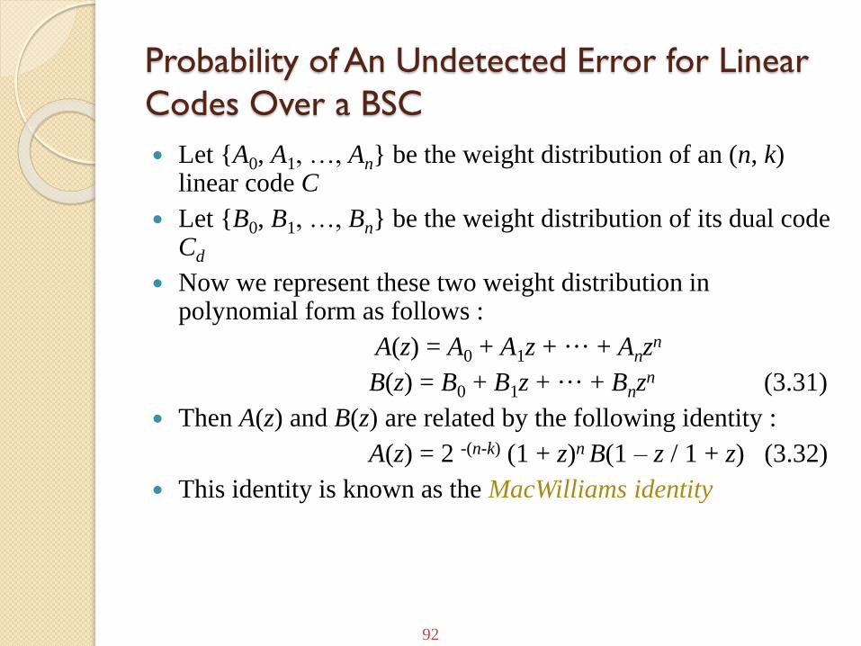
Let {A0, A1, …, An} be the weight distribution of an (n, k) linear code C

Let {B0, B1, …, Bn} be the weight distribution of its dual code Cd

Now we represent these two weight distribution in polynomial form as follows :

A(z) = A0 + A1z + ··· + Anzn

B(z) = B0 + B1z + ··· + Bnzn (3.31)

Then A(z) and B(z) are related by the following identity :

A(z) = 2 -(n-k) (1 + z)n B(1 – z / 1 + z) (3.32)

This identity is known as the MacWilliams identity

93


Codes Over a BSC

The polynomials A(z) and B(z) are called the weight

enumerators for the (n, k) linear code C and its dual Cd

Using the MacWilliams identity, we can compute the

probability of an undetected error for an (n, k) linear

code from the weight distribution of its dual.

From equation 3.19:

1

1

( ) (1 )

(1 ) ( ) (3.33)1

ni n i

u i

i

nn i

i

i

P E A p p

pp A

p

94


Codes Over a BSC

Substituting z = p/(1 – p) in A(z) of (3.31) and using the fact

that A0 = 1, we obtain

Combining (3.33) and (3.34), we have the following

expression for the probability of an undetected error

1

1 (3.34)1 1

in

i

i

p pA A

p p

( ) (1 ) 1 (3.35)1

n

u

pP E p A

p

95


Codes Over a BSC

From (3.35) and the MacWilliams identity of (3.32), we finally obtain the following expression for Pu(E) :

Pu(E) = 2-(n – k) B(1 – 2p) – (1 – p)n (3.36)

where

Hence, there are two ways for computing the probability of an undetected error for a linear code; often one is easier than the other.

If n-k is smaller than k, it is much easier to compute Pu(E) from (3.36); otherwise, it is easier to use (3.35).

0

(1 2 ) (1 2 )n

i

i

i

B p B p

96


Codes Over a BSC

Example 3.10 Consider the (7, 4) linear code given in Table 3.1

◦ The dual of this code is generated by its parity-check matrix

◦ Taking the linear combinations of the row of H, we obtain the

following eight vectors in the dual code

(0 0 0 0 0 0 0), (1 1 0 0 1 0 1),

(1 0 0 1 0 1 1), (1 0 1 1 1 0 0),

(0 1 0 1 1 1 0), (0 1 1 1 0 0 1),

(0 0 1 0 1 1 1), (1 1 1 0 0 1 0)

1110100

0111010

1101001

H

97


Codes Over a BSC

Example 3.10

◦ Thus, the weight enumerator for the dual code is

B(z) = 1 + 7z4

◦ Using (3.36), we obtain the probability of an undetected

error for the (7, 4) linear code given in Table 3.1

Pu(E) = 2-3[1 + 7(1 – 2p)4] – (1 – p)7

◦ This probability was also computed in Section 3.4 using

the weight distribution of the code itself

98


Codes Over a BSC

For large n, k, and n – k, the computation becomes

practically impossible

Except for some short linear codes and a few small

classes of linear codes, the weight distributions for many

known linear code are still unknown

Consequently, it is very difficult to compute their

probability of an undetected error

99


Codes Over a BSC It is quite easy to derive an upper bound on the average probability

of an undetected error for the ensemble of all (n, k) linear systematic

codes

◦ Since [1 – (1 – p)n] ≤ 1, it is clear that Pu(E) ≤ 2–(n – k).

There exist (n,k) linear codes with probability of an undetected error,

Pu(E), upper bounded by 2-(n-k).

Only a few small classes of linear codes have been proved to have

Pu(E) satisfying the upper bound 2-(n-k).

( )

1

( )

( ) 2 (1 )

2 [1 (1 ) ] (3.42)

nn k i n i

u

i

n k n

nP E p p

i

p

100

Hamming Codes

101

Hamming Codes

These codes and their variations have been widely used for error

control in digital communication and data storage systems

For any positive integer m ≥ 3, there exists a Hamming code with

the following parameters :

◦ Code length: n = 2m – 1

◦ Number of information symbols: k = 2m – m – 1

◦ Number of parity-check symbols: n – k = m

◦ Error-correcting capability : t = 1( dmin = 3)

◦ The parity-check matrix H of this code consists of all the nonzero m-

tuple as its columns (2m-1).

102

Hamming Codes

In systematic form, the columns of H are arranged in the

following form :

H = [Im Q]

◦ where Im is an m × m identity matrix

◦ The submatrix Q consists of 2m – m – 1 columns which are the

m-tuples of weight 2 or more

The columns of Q may be arranged in any order without

affecting the distance property and weight distribution of

the code

103

Hamming Codes

In systematic form, the generator matrix of the code is

G = [QT I2m–m–1]

where QT is the transpose of Q and I 2m–m–1 is an (2m – m – 1) ×(2m – m – 1) identity matrix

Since the columns of H are nonzero and distinct, no two

columns add to zero

Since H consists of all the nonzero m-tuples as its

columns, the vector sum of any two columns, say hi and

hj, must also be a column in H, say hl

hi + hj + hl = 0

The minimum distance of a Hamming code is exactly 3

104

Hamming Codes

The code is capable of correcting all the error patterns

with a single error or of detecting all the error patterns of

two or fewer errors

If we form the standard array for the Hamming code of

length 2m – 1

◦ All the (2m–1)-tuple of weight 1 can be used as coset leaders

◦ The number of (2m–1)-tuples of weight 1 is 2m – 1

◦ Since n – k = m, the code has 2m cosets

◦ The zero vector 0 and the (2m–1)-tuples of weight 1 form all the

coset leaders of the standard array

105

Hamming Codes

A t-error-correcting code is called a perfect code if its

standard array has all the error patterns of t or fewer

errors and no others as coset leader

Besides the Hamming codes, the only other nontrivial

binary perfect code is the (23, 12) Golay code (section

5.9)

Decoding of Hamming codes can be accomplished

easily with the table-lookup scheme

106

Hamming Codes

We may delete any l columns from the parity-check matrix H of a

Hamming code

This deletion results in an m × (2m – l – 1) matrix H'

Using H' as a parity-check matrix, we obtain a shortened Hamming

code with the following parameters :

◦ Code length: n = 2m – l – 1

◦ Number of information symbols: k = 2m – m – l – 1

◦ Number of parity-check symbols: n – k = m

◦ Minimum distance : dmin ≥ 3

◦ If we delete columns from H properly, we may obtain a shortened

Hamming code with minimum distance 4

107

Hamming Codes

For example, if we delete from the submatrix Q all the columns of even weight, we obtain an m x 2m-1 matrix.

H’=[Im Q’]

◦ Q’ consists of 2m-1-m columns of odd weight.

◦ Since all columns of H’ have odd weight, no three columns add to zero.

◦ However, for a column hi of weight 3 in Q’, there exists three columns hj, hl, and hs in Im such that hi +hj+hl+hs=0.

◦ Thus, the shortened Hamming code with H’ as a parity-check matrix has minimum distance exactly 4.

◦ The distance 4 shortened Hamming code can be used for correcting all error patterns of single error and simultaneously detecting all error patterns of double errors

108

Hamming Codes

◦ When a single error occurs during the transmission of a code vector, the resultant syndrome is nonzero and it contains an odd number of 1’s (e x H’T corresponds to a column in H’)

◦ When double errors occurs, the syndrome is nonzero, but it contains even number of 1’s.

Decoding can be accomplished in the following manner :

◦ If the syndrome s is zero, we assume that no error occurred

◦ If s is nonzero and it contains odd number of 1’s, we assume that a single error occurred. The error pattern of a single error that corresponds to s is added to the received vector for error correction

◦ If s is nonzero and it contains even number of 1’s, an uncorrectable error pattern has been detected

109

Hamming Codes

The dual code of a (2m–1, 2m–m–1) Hamming code is a (2m–1,m) linear code

If a Hamming code is used for error detection over a BSC, its probability of an undetected error, Pu(E), can be computed either from (3.35) and (3.43) or from (3.36) and (3.44)

Computing Pu(E) from (3.36) and (3.44) is easier

Combining (3.36) and (3.44), we obtain

Pu(E) = 2-m{1+(2m – 1)(1 – 2p)2m-1} – (1 – p)2m–1

The probability Pu(E) for Hamming codes does satisfy the upper bound 2–(n–k) = 2-m for p ≤ ½ [i.e., Pu(E) ≤ 2-m]

error-detecting and error- correcting capabilities of a...

Documents