*ERROR BANDS FOR IMPULSE RESPONSES

Christopher A. Sims

Yale University

and

Tao Zha

University of Saskatchewan

August 1994

* Support for this research was provided in part by National Science Foundation grantnumber SES91-22355. The second author acknowledges research grant support from theUniversity of Saskatchewan.

1. Introduction

For a dynamic system of stochastic equations, impulse responses - the patterns

of effects on all variables of one-period disturbances in a given equation -- are

often the most useful summary of the system’s properties. When the system has been

fit to data, it is important that these responses be presented along with some

indication of statistical reliability, and the literature accordingly contains many

examples of estimated impulse responses shown with error bands. Ingenuity is

required in constructing the bands because the impulse responses are strongly

nonlinear functions of the estimated equation coefficients, and because the estimated

coefficients themselves, in systems fit to nonstationary or near-nonstationary data,

have a complicated classical distribution theory.

Three broad classes of methods have been used to generate error bands for

impulse responses:

methods based on asymptotic Gaussian approximations to the distribution of theresponses;

methods that attempt to develop small-sample classical distributions for theestimated responses, using bootstrap Monte Carlo calculations; and

Bayesian methods that use Monte Carlo methods to find the posterior dis-tribution of the responses.

1The asymptotic methods have both classical and Bayesian interpretations and are

less computationally intensive than the others. However, distributions of impulse

responses often show substantial asymmetry, both in Bayesian posteriors and classical

sampling distributions of estimators, and the asymptotic methods forego from the

start any chance of reflecting the asymmetry. Further, from the classical (but not

the Bayesian) perspective, the asymptotic theory changes character discontinuously at

the boundary of the stationary region of the parameter space, creating difficulties

of interpretation.

---------------------------------------------------------------------------------------------------------------------------------------------------------------------------1Implemented for example in Poterba, Rotemberg and Summers [1993].

1

2The sampling distribution of estimated responses in these models depends

sharply on the true parameter, especially near the boundary of the stationary region,

and the dependence is not even approximately a simple translation of location of the

distribution. This undermines the conceptual basis of the simple interpretations of

bootstrapped distribution theory, which in turn has led to misleading presentation of

results in the literature and to logical errors in generating bootstrapped

distributions.

The Monte Carlo Bayesian confidence intervals are conceptually sound, can

properly reflect asymmetry in the distributions, and are straightforward to3implement, at least for reduced form models. When these methods are extended to

models showing simultaneity, however, technical and conceptual difficulties emerge.

These difficulties, too, have led to logical errors in using Monte Carlo methods to

generate distributions.

The next section of this paper explains why classical and Bayesian inference can

turn out so different in this type of application and shows what is misleading and

mistaken in existing implementations of a bootstrap approach to classical small

sample theory for impulse responses. It documents that in models and data sets like

those used in the economics literature, asymmetry in the distribution of impulse

responses is substantial, and the differences between Bayesian and classical

bootstrap error bands can affect conclusions.

The third section of the paper considers error bands for responses from an

overidentified VAR model, documenting that the differences between correct and

incorrect, and between approximate and exact Bayesian error bands can affect

conclusions. Even more strongly here than in the just-identified models of the

second section, classical bootstrapped error bands, at least as they have in fact

---------------------------------------------------------------------------------------------------------------------------------------------------------------------------2Computed via bootstrap simulation and displayed as error bands in Runkle [1987] andBlanchard and Quah [1989], for example.3The time series analysis program RATS has been distributed since its inception witha procedure that generates by Monte Carlo methods Bayesian confidence intervals forimpulse responses in reduced form VAR systems. These bands are probably the mostcommon in published work, though the fact that they are Bayesian is seldom mentioned.The only classical justification for them is that, if the model is stationary, theywill asymptotically come to match the symmetric intervals implied by the classicalGaussian asymptotic distribution.

2

been implemented, are nearly useless as indicators of uncertainty about impulse

response estimates.

The fourth section gives details of the implementation of our methods, so that

others can check our calculations or use the methods that we suggest in their own

applications.

2. Conditioning on the Data vs. Conditioning on Parameter Values

It is perhaps easiest to approach this issue via the simple two-parameter

univariate AR model discussed in Sims and Uhlig [1992]. As they pointed out, the^asymmetry in the sampling distribution for the least-squares estimatorρ of ρ in the

equation

y(t) = ρ⋅y(t-1) + ε(t) , t=1,...,T , (1)

does not carry over into Bayesian posterior distributions. Any asymmetry in a

Bayesian posterior arises from the prior distribution, and therefore disappears in4large samples. If we assume that the variance ofε is known, it becomes practical

to calculate by Monte Carlo methods an exact classical confidence interval forρ.

Because there is a one-one mapping between the parameterρ and the shape of the^model’s single "impulse response," error bands forρ or ρ correspond directly to

error bands for the impulse response.

q=====================================62 2^We consider the case whereρ=1 and σ =e1/Σy(t-1) =.046, both likely values whenρ

5ρ=.95. An exact finite-sample 68% confidence interval forρ, based on the statistic

---------------------------------------------------------------------------------------------------------------------------------------------------------------------------4Phillips [1992] points out that posteriors from a version of a Jeffreys prior dotend to be strongly asymmetric. However this result only follows if the Jeffreysprior is modified with every increase in sample size, so that the "prior" becomesincreasingly skewed in favor of non-stationarity as the sample size increases.Needless to say, such a procedure, while mechanically resembling Bayesiancalculations, is not one that would be recommended by most Bayesians. So long as theprior does not change with sample size and has a continuous p.d.f. in theneighborhood of the true parameter, asymmetry in the posterior will tend to lessen assample size increases.5Since the classical small sample distribution was calculated by Monte Carlo methodson a grid with spacing .01 on theρ-axis and with just 1000 replications, "exact"should be in quotes here, but the accuracy is good enough for this example. Themethod was to construct for eachρ 1000 artificial samples for y generated by (1)with T=60 variance ofε equal to 1, and y(0)=1. (The same sequence ofε’s was used

3

ρ/σ , is (.919,1.013). A Bayesian posterior 68% confidence region is justρρ±σ =(.904,.996). The 16th and 84th percentiles (bounding a 68% probability band)ρ

^for ρ given ρ=.95, computed by Monte Carlo simulation, is (.867,.973). Figure 1

plots the maximum likelihood estimated impulse response together with the error bandssfor the impulse response,ρ , implied by these three bands forρ. (The classical

^probability band for the distribution ofρ is labeled the "bootstrap" band in the

figure.) Note that while the classical confidence band is somewhat asymmetric^initially, reflecting the asymmetry in the distribution ofρ, the asymmetry increases

with the time horizon of the response because of the nonlinearity of the mapping from

ρ to the response path. The classical 68% probability band for the distribution ofsthe response lies somewhat more below than above .95 , the opposite of the behavior

of the classical confidence band.

Computing the bootstrap band for the estimate in Figure 1 requires only^generating a Monte Carlo sample from the distribution ofρ given ρ=.95. The

classical confidence band requires repeating such a calculation for many values ofρ.6If computational resource constraints preclude such an ambitious calculation, seeing

a band such as the bootstrap band in Figure 1 is of questionable value as a

substitute. In this case, for example, it might correctly give us the idea that a

confidence band probably lies more above than below the estimated response, but the

asymmetry in the bootstrap band is so much weaker than the oppositely oriented

asymmetry in the confidence band that the effect might be on the whole misleading.

Moreover, in published work using bootstrapping to generate information about the

distribution of impulse responses, it appears that researchers have presented

probability bands based on single true parameter values, like the bootstrap band in

Figure 1, without providing any clear indication to the reader that these are not

---------------------------------------------------------------------------------------------------------------------------------------------------------------------------

for all ρ’s on each draw of anε sequence.) For eachρ, an empirical distribution of^the t-statistic (ρ-ρ)⋅sqrt(Σy(t)y(t-1)) was constructed and the 16% and 84% quantiles

of the empirical distribution calculated. Then a classical 68% confidence intervalcan be constructed in a particular sample as the set of allρ’s for which the t-statistic lies between the 16% and 84% quantiles appropriate for thatρ.6In a multivariate model matters are much worse, as everyvector of parameter valuesimplies a different distribution of all the impulse responses. Even though we areinterested in a one-dimensional confidence band, computing it requires consideringhow the distribution varies over the whole multi-dimensional parameter space.

4

7confidence bands. The fact that, for short horizons where the mapping from

coefficients to responses is not strongly nonlinear, any tendency of these bands to

lie above or below the estimated response implies an opposite tendency in a true

confidence band is not mentioned.

The Bayesian band also shows some asymmetry, but here it is due entirely to thesnonlinearity of the mapping fromρ to ρ , as the Bayesian posterior forρ itself is

^symmetric about ρ. It is not very different from the classical band at the lower

side, but is quite different at the upper side because the Bayesian posterior gives

considerably less weight to explosive models than does inference based on hypothesis

testing.

This simple example displays most of the themes we will elaborate in the

remainder of the paper: the strong asymmetry in reasonable error bands for impulse

responses; the lack of any simple rule for translating small sample distribution

theory generated from a single parameter value into information about the shape of an

actual confidence band; and the moderate behavior of Bayesian error bands.

Econometricians are well accustomed to the idea that, in a standard linear

regression model with exogenous regressors

y = Xβ + ε (2)

^it makes sense to use the distribution of the estimateβ of β conditional on the^observed value of X, not the unconditional distribution ofβ, even if X has a known

probability distribution. If we happen to have a sample in which X′X is unusually

large, the sample is unusually informative. Where X′X is unusually small, the sample

is unusually uninformative. We want our standard errors to reflect the difference

between informative and uninformative samples, not to give an average of precision

across informative and uninformative samples. Bayesian and standard classical

inferential procedures agree on this point. But if in (2) X is a vector with

elements X(t)=y(t+1) so that the model becomes equation (1), Bayesian and classical

analyses part company.

---------------------------------------------------------------------------------------------------------------------------------------------------------------------------7This is true of Runkle [1987] and Blanchard and Quah [1989].

5

It remains possible in such a dynamic model to have informative and

uninformative samples. We can get many values of y(t) that are large in absolute

value, allowing us to determineβ with small error, or we may be unlucky and draw

only values of y(t) that are near zero, in which case it will be hard to determineβprecisely. Bayesian analysis is based on the likelihood and is always conditional on

the actual sample drawn. It has no problem distinguishing informative from

uninformative samples and adjusting its conclusions accordingly. But the device that

allows classical analysis to conform to Bayesian conclusions in the presence of

exogenous random X is not available for a dynamic model. One cannot condition on the

right-hand-side variables -- that is, hold them fixed -- while allowing the left-

hand-side variable to vary randomly. The left-hand side variables, with one

exception at the end of the sample,are right-hand side variables. The best a

classical procedure can do is to condition on y(0) (assuming that is the first

observed value of y), using the conditional distribution of y(1),...,y(T) given y(0)

for making probability statements. But this forces the estimated precision of an

estimator, for example, to be an average across informative and uninformative-1 ^samples. It is as if instead of using (X′X) as the estimated variance ofβ in our

-1exogenous-regressor example we usedE[(X ′X) ], even in cases where the actual-1(X′X) is much bigger or smaller than the expectation.

It is probably due to recognition of this point that Blanchard and Quah [1989]

arrived at a version of a bootstrap procedure for forming error bands on impulse

responses that approximately holds constant the "informativeness" of Monte Carlo

sample draws, but in the end has no apparent justification from either a classical or8a Bayesian perspective. They intended to implement a bootstrap procedure, in which

estimated parameter values are taken as exact and artificial random samples are

generated by drawing sequences of residuals from the empirical distribution function

of the estimated residuals. Doing this correctly in a first-order vector AR system

---------------------------------------------------------------------------------------------------------------------------------------------------------------------------8We criticize Blanchard and Quah here with reluctance. We understood the defects oftheir procedure only after considerable thought. They co-operated with us fully aswe attempted to understand and duplicate what they had done, even supplying us witharchived computer code for their original calculations. And their work attracted ourattention because it was unusually ambitious in attempting to use a classicalinferential framework without ignoring asymmetry in the error bands. Even though itturns out to have contained mistakes, their work was pathbreaking.

6

like (1), for example, requires generating artificial random draws of y(1) through*y(T) (where T is sample size) recursively. A given bootstrap random sequence y

starts off with

^* ^*y (1) = ρ⋅y(0) + ε (1) , (3)

*where the vectorε (1) is a draw from the empirical c.d.f. of the estimated residuals^and ρ is the estimated parameter matrix. Then

^* * ^*y (t) = ρ⋅y (1) + ε (t) , t=2,...,T . (4)

^ ^*The bootstrapped distribution forρ is based on the distribution of the estimatesρ*formed from the y sequences.

But this procedure makes clear the unattractive fact that the distribution

theory generated this way averages together the behavior of the estimator in

informative and uninformative samples. It does not make sense to quote error bands

on our estimates that allow for the possibility that we could have had a less

informative sample than we actually do. Possibly in recognition of this point,

Blanchard and Quah generate their artificial random samples of y(1),...,y(T) as9 ^follows. They first form a sequence y(t) using the formula

^y(t) = ρ⋅y(t-1), t=1,...,T . (5)

*They form a typical random sequence y using

^ ^* ^*y (t) = ρ⋅y(t-1) + ε (t) . (6)

*This method ensures that the randomly drawn y sequences will all have the same

general shape as the actual data sequence y. If we have an informative sample of

actual data y, in which y takes on large values relative to the standard deviation of* *ε, all the y sequences will share this character. However, the y sequences

^generated this way do not satisfy the original model. Even ifρ happened to match* *the true value ofρ, the conditional expectation of y (t) given data on y (s) for s<t

*would not be ρ⋅y (t-1). Across this random sample of y sequences, the conditional^* ^ *expectation of y (t) is the constantρ⋅y(t-1). The lagged value y (t–1) differs from

---------------------------------------------------------------------------------------------------------------------------------------------------------------------------9Quah generously provided us with the code used to generate error bands for thearticle. We were able to duplicate the published error bands by using our ownimplementation of the algorithm we describe here.

7

y(t-1) by a random "error" term, so that estimates ofρ based on these artificial

samples are biased, even asymptotically.

But even were they computed correctly, the way error bands based on the

bootstrap have been presented in the literature is misleading, both in Blanchard and

Quah’s work and in others’. Consider Figure 2.1. This displays our computations of

the Blanchard-Quah impulse responses and error bands. Notice that the bands around

the responses to a demand shock lie almost entirely between the estimated response

and zero, while those around the responses to supply shocks lie almost entirely on10the opposite side of the estimated response from 0. A naive reader might be tempted

to conclude that, since these are characterized as one-standard-deviation bands, the

responses to supply shocks are strongly "significantly" different from zero --

probably even bigger than suggested by the point estimates -- while the responses to

demand shocks are probably smaller than suggested by the point estimates, though

still apparently "significantly" different from zero over most of their range.

But this interpretation treats the bootstrapped error bands as if they were the

same kind of 68% confidence interval that a± one standard error band around a sample

mean would be. These bands are not, taken on their own terms, classical confidence

intervals. They show that if the true coefficients of the model matched the

estimates, then with high probability the estimated response to demand shocks would

be smaller than the true ones and the estimated responses to supply shocks would be

larger than the true ones. This suggests that the estimated responses to demand

shocks are probablysmaller than the true ones and the estimated responses to supply

shocks probablylarger than the true ones -- the opposite of the conclusion implied

by naive treatment of the "error bands" as confidence intervals.

These heavily skewed error bands reflect in part the bias induced by Blanchard

and Quah’s mistaken implementation of the bootstrap. Figure 2.2 shows the results of

a similar calculation based on a correct bootstrap. The bias in the response of Y to

---------------------------------------------------------------------------------------------------------------------------------------------------------------------------10These bands are not simply lines lying one standard deviation on either side of themean of the bootstrapped distribution of the responses. The bias is so strong thatin many cases bands computed that way would not include the estimated response path!To maintain comparability with Blanchard and Quah, we follow them in generatingFigures 2.1 and 2.2 by a method that forces the error band to contain the originalestimated response. We give a complete description in the section on methods below.

8

a supply shock is seen to be reversed, while that in the response of U to a supply

shock is largely gone. The biases in responses of Y and U to demand shocks remain of

the same sign as before, but are much weaker, except at the peaks of the response

curves. Important asymmetry remains: the estimated response of output to the supply

shock, for example, can be seen to be much more likely to deviate downward from its

true value than upward. If the plotted band were a± one standard error confidence

interval, this response might appear to be "insignificantly" different from zero, but

when the asymmetry is properly interpreted that implication is reversed. Similar

points apply to the skewed bootstrap bands for responses to demand shocks.

A similar misinterpretation of a bootstrapped distribution of responses appears

in Runkle [1987]. There error bands around impulse responses are not at issue, but

instead error bands for distributions of variance decompositions. The lower bounds

of probability intervals for bootstrapped elements of the variance decomposition11tables are interpreted as if they were lower bounds of confidence intervals.

In Figure 2.3 we display one-standard error bands about the maximum likelihood

estimates for the Blanchard-Quah model based on the Bayesian posterior distribution12under a prior that is in a certain sense "flat". Note that here the band for the

response of output to a supply shock is less asymmetric than for either the correct

bootstrap or the original Blanchard-Quah procedure. What asymmetry there is in the

band for that response is the reverse of that in the correct bootstrap, as would be

expected if the Bayesian interval were simply undoing the bias in the bootstrap

interval. But the bands for responses to demand shocks are still, in the

neighborhood of their peaks, asymmetric in the same direction as the two bootstrap

bands.

---------------------------------------------------------------------------------------------------------------------------------------------------------------------------11Putting confidence bands on variance decompositions is probably not a good idea inthe first place, as variance contributions are non-monotone functions of underlyingresponses. Usually when the estimate of a response is positive, say, we do not meanto count possible negative responses as contributing to the "significance" of theeffect displayed in the positive response. Confidence bands on variancedecompositions may in effect do this. Variance decomposition point estimates can behelpful in summarizing impulse responses, but confidence bands on the responsesthemselves are much more useful than bands on the variance decompositions.12Details of the algorithm are in the section on methods below.

9

None of the bands displayed in Figures 2.1-2.3 have any claim to being even

approximate classical confidence intervals. For the Bayesian bands this is because13they are not based on classical reasoning. For the correctly computed bootstrap

bands this is because the bands only characterize the distribution of the estimated

response under one particular assumption about the true coefficients of the dynamic

equation system. In simpler contexts, the bootstrap can generate asymptotically

justified confidence regions because, in large samples, the distribution of the

estimator is normal and depends on the true value of the parameter only via a^"location shift". That is, if the true parameter value isβ and the estimator isβ,

^the distribution of β-β does not depend much onβ in large samples. But this is not

true for dynamic models that allow for non-stationarity. In a multivariate model

with several possible unit roots, the dependence on the true model parameters of the

distribution of estimated responses about the true responses is strong and compli-

cated. Its full nature must be traced out in order to generate an accurate

confidence region or interval. Doing so would require repeating the bootstrap

distributional calculations for every point on a fine grid of true values of the

system’s coefficients.

Nonetheless it may be interesting to see how far the coverage probabilities of

intervals like these are from being the 68.3% we would expect for± one standard

error bands in a simpler setting. To examine this point, we consider a bivariate

reduced form VAR relating real GNP (y) to M1 and estimated from quarterly data over141948:1-1989:3. Figure 3.1 shows the estimated impulse responses for this system

together with one-standard-error bands generated as the sample mean of the bootstrap

---------------------------------------------------------------------------------------------------------------------------------------------------------------------------13Actually, there is some reason to hope that Bayesian 68% confidence regions mightalso turn out to be not far from having that coverage probability when analyzed asclassical interval estimators. A Bayesian 68% interval must have a 68% chance ofcontaining the truth when we average across different true parameter values,weighting by the prior. It may have a much higher or lower coverage probability forsome particular true parameter value, but it can’t be off in the same directioneverywhere.14We switch to this model from the Blanchard-Quah model at this point because the BQmodel requires solving a small nonlinear system at each estimation. The calculationsof coverage probabilities absorb many hours of computer time even for the bivariatereduced form model, and would be prohibitive (without moving to a much biggercomputer system) for the BQ model. The data we used for this calculation, togetherwith other data and code used in generating results in this paper, will be availableby anonymous ftp in directory ######## on the econ.yale.edu computer system.

10

distribution ± one standard error. We also tried generating the bands as the 16th

and 84th percentiles of the bootstrapped distributions of the estimates, and the

resulting graphs are almost indistinguishable by eye from those generated as the mean

± one standard error and shown in Figure 3.1. Observe that, though there is little

apparent bias in the distribution of the cross responses of M1 to Y-innovations and

vice versa, there is strong bias toward zero in the responses of Y and M1 to their

own innovations. Figure 3.2 shows the± one standard deviation confidence band of a

Bayesian posterior distribution for these responses. As with the bootstrapped bands,

computing these as the 16th and 84th percentile of the distribution instead of as the

mean ± one standard deviation resulted in almost identical graphs. For the two cross

responses the posterior confidence bands are similar in size and location to the

bootstrapped bands. For the own responses, however, the bias toward zero is gone,

replaced by a smaller bias upward. In accord with common sense, the fact that there

is strong downward bias in the estimated responses results in a Bayesian posterior

band that puts more probability above than below the maximum likelihood estimate.

Table 1 shows the results of Monte Carlo calculations of the coverage

probabilities of the bootstrapped bands. If these were ordinary± one standard

deviation confidence bands we would expect the coverage probability to be .683, and

indeed for the two cross responses, where there is little bias in the estimates, the

coverage probabilities are very close to the expected .683. (The coverage

probability of 1 for the first term in the response of M1 to y reflects the fact that

this response is always constrained to zero by the orthogonalization.) For the

biased own responses, not surprisingly, the coverage probabilities are much lower

than .683. Note that, since these coverage probabilities are estimated from 600

Monte Carlo trials (each of which itself entails 400 Monte Carlo draws for the

bootstrap intervals), the Monte Carlo sampling error in the coverage probability has

a standard deviation on the order of .02.

Table 2 shows the coverage probabilities of the Bayesian intervals. These are

about as close to .683 for the cross-responses as are those for the bootstrap bands,

while being much closer to .683 for the own responses. Since they are not classical

confidence intervals, however, their coverage probabilities are not exactly .683,

instead being somewhat lower. Note that this does not mean that the Bayesian

11

intervals are flawed and should be corrected by widening or further upward shifting

to make a stronger allowance for bias. The Bayesian intervals are constructed to

represent reasonable probability statements about the location of the true parameter

given the data, taking account of the fact that the true parameter value is unknown.

The coverage probabilities are probabilities that, in repeated samples, the interval

will contain the true value of the response, when the true parameter vector of the

model is held fixed at one particular value -- in the case of these graphs, the

parameter vector estimated from the original data. A classical confidence interval

constructed to obtain 68.3% coverage for every possible true parameter value will

generally have a conditional probability different from 68.3% for some possible15realizations of the sample data, regardless of the prior distribution. This

corresponds to the dual fact that a Bayesian 68.3% confidence interval will generally

have a coverage probability, conditional on the true value of the parameter vector,

different from 68.3% for some possible parameter vectors. In some contexts, the two

kinds of intervals turn out to be approximately or even exactly the same. But in

these dynamic models the intervals are inevitably different, and where the two

interpretations conflict it is hard to see what argument there can be for preferring

the classical one.

3. Simultaneity

The Blanchard-Quah model is an example of an "identified VAR". That is, it

gives the reduced form forecast error for a set of time series observations an

explicit interpretation in terms of underlying behavioral disturbances. The model is

exactly identified, meaning that the restrictions that yield the interpretation are

just adequate to produce a one-one mapping between the set of possible reduced form

models and the set of possible behavioral interpretations. Thus the standard

Bayesian procedure for generating error bands on VAR impulse responses, which is

distributed as a pre-packaged procedure with the RATS time series analysis program,

can easily be adapted to produce Bayesian error bands for the Blanchard-Quah model.

---------------------------------------------------------------------------------------------------------------------------------------------------------------------------15Of course in any particular sample a classical confidence interval will be just aset of points, and there will be some prior for which this set of points hasposterior probability matching the classical coverage probability. But generallythere is no single prior that will in this way rationalize the classical interval forall possible samples.

12

The RATS procedure generates random draws from the joint posterior distribution of

the covariance matrix of innovations and the reduced form coefficient matrix. In its

packaged form, it uses these draws to generate impulse responses from a triangular,

or Choleski, decomposition of the covariance matrix of innovations. Instead one can

use the Monte-Carlo draw of the innovation covariance matrix and coefficient matrix

as if they were estimates to derive the corresponding estimated structural model and

impulse responses. Since in an exactly identified model the procedure used to derive

estimates of the structure from estimates of the reduced form just implements the

one-one mapping from true reduced form parameters to true structure, the Monte Carlo

procedure outlined above works to produce a draw from the posterior distribution of

the structural responses.

It seems natural to handle the case of overidentification, where the behavioral

model has enough restrictions so that not all reduced form specifications are

consistent with the model, by the same method. One uses the RATS procedure to

generate draws from the covariance matrix of innovations and the reduced form

coefficients, uses the appropriate estimation procedure to derive from these the

implied structural model, then generates impulse responses from that. Indeed this is

just what Gordon and Leeper [1994] do with their overidentified model. But the draw

from the distribution of reduced form parameters generated by the RATS procedure

ignores the overidentifying restrictions on the covariance matrix of innovations.

Mapping draws from this unrestricted distribution into draws of the structural

coefficients via the estimation procedure does not produce a draw from the posterior

distribution of the structural parameters. This does not necessarily mean that the

error bands it produces in any particular application are badly misleading. The

procedure is correct in the limiting case of exact identification, and

overidentifying restrictions may be weak, so that results are little affected by

taking proper account of the overidentification. But this is like estimating a

simultaneous equations model by least squares -- the results may not be too bad in

any particular application, but the practice is unjustifiable, and badly mistaken

conclusions are possible.

A correct Monte Carlo procedure for generating error bands in this situation

requires either drawing parameters directly from the posterior distribution of the

13

overidentified model, or else weighting draws from some other more convenient

distribution so that the bands accurately reflect the true distribution. We describe

in detail a method for constructing correctly weighted draws in our section on

methods, below. Another, more easily implemented, possibility is to draw directly

from the approximate posterior generated from a second-order Taylor expansion of the

posterior p.d.f. about its peak. (This approximation can also be thought of as the

Gaussian asymptotic distribution of the parameter estimates when the model is

stationary.)

For a pair of 6-variable overidentified macroeconomic models in a paper

previously published by one of us in 1986, we have computed error bands by the

apparently natural but incorrect Bayesian method, by Monte Carlo draws properly

weighted to reflect the exact posterior distribution (under Gaussian assumptions on

the distribution of disturbances), by Monte Carlo draws from the Gaussian

approximation, and by a bootstrap procedure. In one of these models (the two models

are called two "identifications" in the original paper) all the candidate Bayesian

methods -- even the incorrect one -- deliver confidence bands of nearly the same size

and location. For this model, the Bayesian bands were also nearly symmetric about

the estimated response. Bootstrap bands showed strong bias and were clearly

different from the Bayesian bands. We do not show the results for this model, called

identification 1 in the original paper, because all the differences between methods

it produced appear in stronger form with the other model, identification 2.

Nonetheless it is important to note that results like those for identification 1 are

possible. The fact that in some models the extra computational resources required to

compute the correct bands produce little change in results does not imply that this

will be generically true.

Figure 4.1 shows the impulse responses and error bands for the full 6-variable

system, with the bands computed, by importance-sampling weighted Monte Carlo methods,

as the exact small-sample Bayesian posterior one-standard-deviation intervals. None

of the bands shows any strong asymmetry about the estimated response. The important

responses for interpretation of the model are those in the first two columns. The

responses to money supply shocks (MS, first column) fit most economists’ beliefs

about the effects of a monetary contraction: interest rates rise, money stock falls,

14

output falls, prices fall, unemployment rises, and investment drops. Most of these

responses are more than two standard deviations away from zero over at least part of

the plotted time horizon, with the response of prices and investment being

exceptions. The responses to the identified money demand shocks (MD, second column)

contain one interpretive problem: A rise in demand for money produces a strong,

positive response in prices that is more than two standard deviations above zero over

most of the plotted range.

Figure 4.2 shows the responses to MS and MD with error bands computed by the

computationally cheaper method of unweighted sampling from the asymptotic Gaussian

approximation to the posterior. It produces results generally consistent with those

of the exact small sample posterior, but here the band for responses to MD by y and P

shows substantial asymmetry, of a sort that probably would influence conclusions.

Both bands are shifted toward zero, making both the (a prior expected) negative

effect of MD on output and the (a priori unexpected) positive effect of MD on prices

appear to be less than two standard deviations away from zero over most of the

plotted range.

Figure 4.3 shows results from the incorrect adaptation of the method appropriate

for reduced forms. The bias in Figure 4.2 reappears here, more strongly.

16Figure 4.4 shows bands computed by a correct bootstrap. Several of these bands

show such strong bias that they lie entirely above or below the estimated response

over part of the plotted range. The biases for the crucial responses of y and P to

MD are very strong here. The naive interpretation of the bootstrapped bands as if

they were confidence intervals might make it appear that not even one of the

responses to MS are "significantly different from zero". The same would be true for

responses of Y and P to MD. But it is interesting that the less naive interpretation

of these intervals, recognizing that they show bias that needs to be corrected for,

would also be mistaken. The P response to MD in the second column shows that, if the

estimated model were true, there is about a 68% probability that the estimated

response of P to MD would lie below the true response. One might think this suggests

---------------------------------------------------------------------------------------------------------------------------------------------------------------------------16Since in this graph comparability to Blanchard and Quah is not important, here weshow the bootstrapped intervals as one-standard-deviation bands about the mean of thebootstrapped distribution.

15

that there is a 68% chance that the true response lies above the large positive

estimated response, so that that response is very strongly "significantly different

from zero." But referring back to Figure 4.1 we see that the conclusion that the

true response is more likely above than below the estimated response is not correct.

When the dependence of the distribution of the response on the true parameter value

is fully taken into account, allowing not just for bias but also dependence of

precision on the level of the response, we find that a reasonable confidence band is

more or less symmetric about the estimated response, not skewed above it or below it.

But this Bayesian posterior confidence interval is narrower than the bootstrapped

interval, so that the positive response of P to MD is in fact precisely estimated.

4. Methods

A. Just-Identified Models

All the models we consider are special cases of the following one:

G(L)y(t) = ε(t) , (6)

where y(t) is an m×1 vector of observed variables, G(L) is an m×m matrix polynomial0in non-negative powers of the lag operator, G , the coefficient of L in G, is non-0

singular, andε(t) is an m×1 vector of disturbances. We assume

q e q eE2ε(t)ε(t)′y(t-s), all s>02 = Λ, E2ε(t)y(t-s), all s>02 = 0, all t, (7)z c z c

with the matrix Λ diagonal. Because G is non-singular, if we strengthen the second0part of (7) to independence ofε(t) from past y’s, the model is a complete

description of the conditional distribution of y(t+1) given y’s dated t and earlier

and the distribution ofε(t).

-1The model has a reduced form obtained by multiplying (6) on the left by G to0produce

B(L)y(t) = u(t) (8)

in which B =I and u(t), though still uncorrelated with past y’s, no longer has a0diagonal covariance matrix. Instead

q e -1 -1′E2u(t)u(t)′y(t-s), s>02 = Σ = G ⋅Λ⋅G . (9)0 0z c

16

With the disturbance u Gaussian, the likelihood function for {B,Σ} conditionalton the actual initial values of y is proportional to q, defined by

q e( )2 2-T/2 2 -12q(B,Σ) = Σ ⋅exp2tr2S(Β)Σ 22 (10)2 2

2 29 0z c

u(t;B) = B(L)y(t) (11)Ts ^ ^S(B) = u(t,B)⋅u(t,B)′ . (12)t

t=1

It turns out to be convenient to choose the prior forΣ to be flat in Jeffreys’

sense, rather than flat in the elements ofΣ itself, meaning that we multiply the-(m+1)/2 17likelihood by Σ before treating it as a posterior p.d.f.

We consider first the case where there are not enough a priori restrictions on G

to imply any restrictions on either B orΣ. Then because the likelihood has a

Gaussian form as a function of B alone (i.e. the log likelihood is quadratic in B

alone), the marginal posterior pdf forΣ is easily computed by integrating over B to

obtain the form:

q e( )2 2-(T+m-ν+1)/2 1 2 ^ -12p(Σ) ∝ Σ exp2- ----- tr2S(B)Σ 22 , (13)

2 2 22 29 0z c

where ν is the number of estimated coefficients per equation. This is the p.d.f. of18an inverted Wishart with T-ν degrees of freedom. A draw forΣ from the inverse

---------------------------------------------------------------------------------------------------------------------------------------------------------------------------17The Jeffreys prior for a model that has data X dependent on a parameterβ via a

‘ ‘q e2 2.5

2 2 2222 2d log(p(X;β)2 2p.d.f. p(X;β) for X is 2E ------------------------------------------------------ 2 . It has the property that if we set adβ⋅dβ′2 2 22

2 2z c2 2% %

Jeffreys prior under one parameterization, then transform to a different parameterspace in assessing the posterior, the result is just as if we had begun with aJeffreys prior on the transformed parameter space. We do not follow Phillips [19 ]in using a Jeffreys prior on B andΣ jointly for two reasons. One is that the jointJeffreys prior is messier to work with than a flat prior, not easier. Another isthat the joint Jeffreys prior changes with initial conditions and with sample size,making it difficult to maintain comparability across applied studies when they usethe joint Jeffreys prior.18Box and Tiao [1973] define the degrees of freedom for the Wishart differently from

17

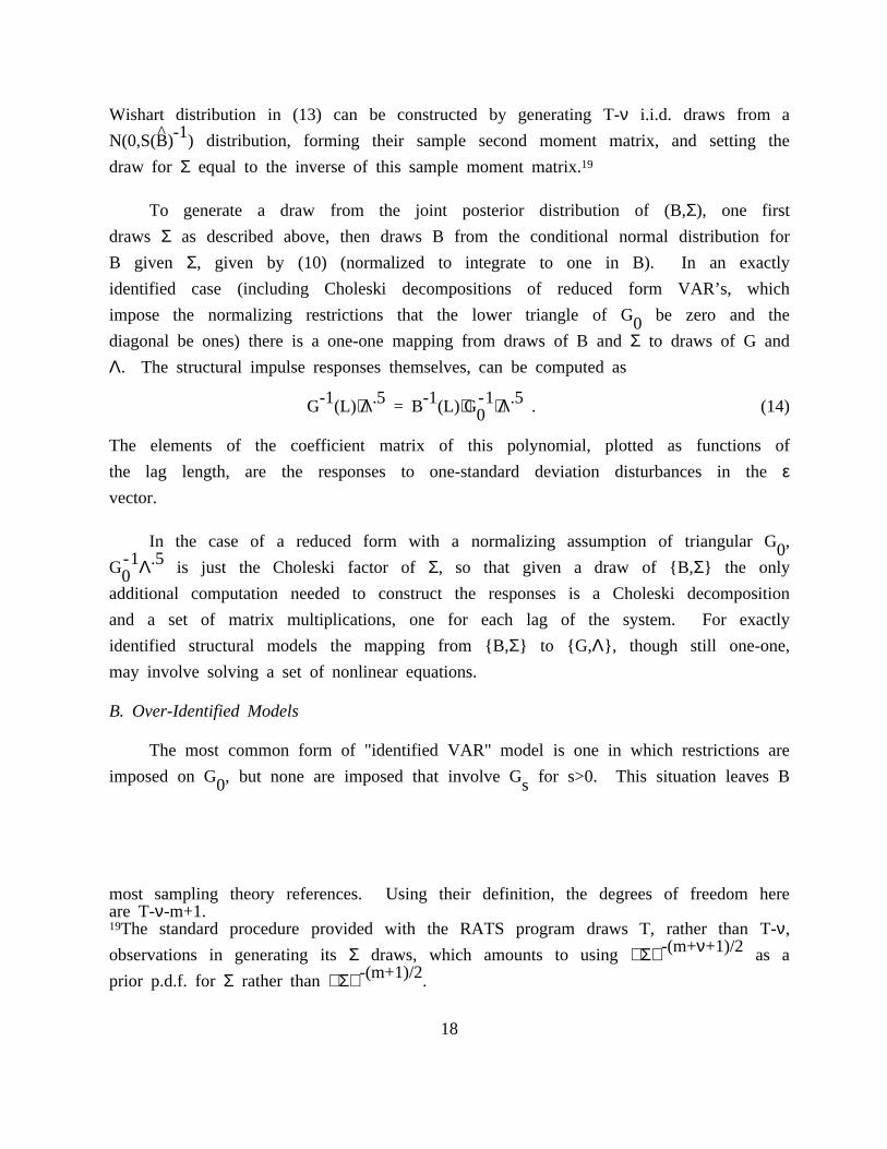
Wishart distribution in (13) can be constructed by generating T-ν i.i.d. draws from a^ -1N(0,S(B) ) distribution, forming their sample second moment matrix, and setting the

19draw for Σ equal to the inverse of this sample moment matrix.

To generate a draw from the joint posterior distribution of (B,Σ), one first

draws Σ as described above, then draws B from the conditional normal distribution for

B given Σ, given by (10) (normalized to integrate to one in B). In an exactly

identified case (including Choleski decompositions of reduced form VAR’s, which

impose the normalizing restrictions that the lower triangle of G be zero and the0diagonal be ones) there is a one-one mapping from draws of B andΣ to draws of G and

Λ. The structural impulse responses themselves, can be computed as

-1 .5 -1 -1 .5G (L)⋅Λ = B (L)⋅G ⋅Λ . (14)0

The elements of the coefficient matrix of this polynomial, plotted as functions of

the lag length, are the responses to one-standard deviation disturbances in theεvector.

In the case of a reduced form with a normalizing assumption of triangular G ,0-1 .5G Λ is just the Choleski factor ofΣ, so that given a draw of {B,Σ} the only0additional computation needed to construct the responses is a Choleski decomposition

and a set of matrix multiplications, one for each lag of the system. For exactly

identified structural models the mapping from {B,Σ} to {G, Λ}, though still one-one,

may involve solving a set of nonlinear equations.

B. Over-Identified Models

The most common form of "identified VAR" model is one in which restrictions are

imposed on G , but none are imposed that involve G for s>0. This situation leaves B0 s

---------------------------------------------------------------------------------------------------------------------------------------------------------------------------

most sampling theory references. Using their definition, the degrees of freedom hereare T-ν-m+1.19The standard procedure provided with the RATS program draws T, rather than T-ν,

-(m+ν+1)/2observations in generating itsΣ draws, which amounts to usingΣ as a-(m+1)/2prior p.d.f. for Σ rather thanΣ .

18

unrestricted in the reduced form, no matter how strongly restricted is G . In this0case we can reparameterize in terms of G ,Λ and B, so that (10) becomes, using (9),0

q e( )2 2

T -T/2 1 2 -12′LH ∝ G Λ exp2- ----- tr2G SG Λ 220 2 2 0 0 22 29 0z c

q e( )2 21 2 ^ ^ ′ -1 2

K exp2- ----- tr2(B-B)′X′X(B-B)G Λ G 22 (15)2 2 0 022 29 0z c

where X is a matrix of given observations in the reduced-form. With a flat prior on-1B and G and a Jeffreys ignorance priorΛ on Λ , the joint posterior pdf is simply0

the likelihood function (6) multiplied byΛ. The distribution of B conditional on-1G and Λ is normal; the distribution of each element ofΛ conditional on G is of0 0

one-dimension Wishart form or general chi-square distribution. The marginal-1posterior pdf for G after integrating out B andΛ is of the form:0

( )2 m 2-(T-ν)/22 2T-ν pp(G ) ∝ G 2 σ 2 (16)0 0 q i2 22i=1 29 0

′where σ is the i’th diagonal element of the matrix G SG . Note thatG is, withi 0 0 0all elements of G fixed except the ij’th,γ , a linear function of γ . At the0 0ij 0ijsame time an individualγ enters only σ , not σ for k≠i, and it does so0ij i kquadratically. Thus, considered as a function ofγ alone, the posterior p.d.f. in0ij(7) is 0(1) as γ L∞, so long as γ affects G at all. Of course there is a0ij 0ij 0leading case in which this flat-prior posterior is proper---------- when G is triangular0and normalized to have ones down the diagonal, its determinant is identically one.

But in general the flat-prior posterior on the elements of G is improper, for all0sample sizes. This does not mean Bayesian inference is sensitive to the proper prior

regardless of sample size. The concentration of the likelihood near the peak

increases with sample size, so that for any given smooth, proper prior, the posterior

in large samples becomes independent of the shape of the prior. We would expect,

however, that inference might be more sensitive to the behavior of the prior in the

tails than in standard cases. Because of the assumed orthogonality of structural

disturbances, this model is not a standard simultaneous equations model. However the

19

non-integrable likelihood, as well as the fact that we can remedy this behavior of

the likelihood by reparameterizing as shown below, are very similar to results by van

Dijk [ ] and by Chao and Phillips [1994] for the standard simultaneous equations

model.

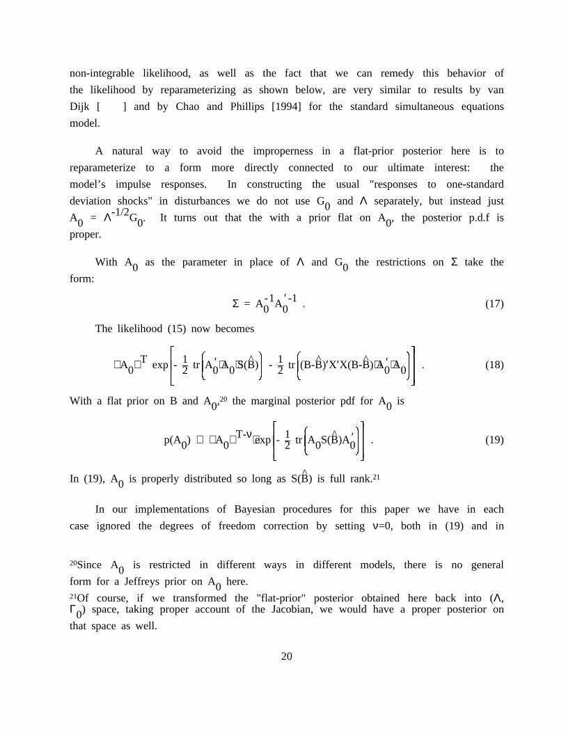
A natural way to avoid the improperness in a flat-prior posterior here is to

reparameterize to a form more directly connected to our ultimate interest: the

model’s impulse responses. In constructing the usual "responses to one-standard

deviation shocks" in disturbances we do not use G andΛ separately, but instead just0-1/2A = Λ G . It turns out that the with a prior flat on A , the posterior p.d.f is0 0 0proper.

With A as the parameter in place ofΛ and G the restrictions onΣ take the0 0form:

-1 ′ -1Σ = A A . (17)0 0

The likelihood (15) now becomes

q e( ) ( )2 2T 1 2 ^ 2 1 2 ^ ^ 2′ ′A exp2- ----- tr2A ⋅A ⋅S(B)2 - ----- tr2(B-B)′X′X(B-B)⋅A ⋅A 22 . (18)0 2 2 0 0 2 2 2 0 02

2 29 0 9 0z c

20With a flat prior on B and A , the marginal posterior pdf for A is0 0q e

( )2 2T-ν 1 2 ^ 2′p(A ) ∝ A ⋅exp2- ----- tr2A S(B)A 22 . (19)0 0 2 2 0 022 29 0z c

^ 21In (19), A is properly distributed so long as S(B) is full rank.0

In our implementations of Bayesian procedures for this paper we have in each

case ignored the degrees of freedom correction by settingν=0, both in (19) and in

---------------------------------------------------------------------------------------------------------------------------------------------------------------------------20Since A is restricted in different ways in different models, there is no general0form for a Jeffreys prior on A here.021Of course, if we transformed the "flat-prior" posterior obtained here back into (Λ,Γ ) space, taking proper account of the Jacobian, we would have a proper posterior on0that space as well.

20

the reduced form setup (13). This keeps our work comparable to all the existing work

that uses the RATS packaged procedure on the reduced form (since that procedure also

uses ν=0), but we have mixed feelings about perpetuating this practice. Of course

flat priors of any variety have an element of arbitrariness, but settingν=0 in theν -(m+ν+1)/2formulas for the posterior implies a prior of the formA or Σ . This0

asserts greater confidence that residual variance is small in larger models, which

may not be an appealing assumption. It may be worth noting that withν=0, (19) is

just the likelihood concentrated with respect to B.

Unlike the analogous (13) in the reduced form case, (19) is not in general of

the form of any standard p.d.f. To generate a sample from it, our procedure was to

begin with draws from the p.d.f. generated from a second-order Taylor expansion of

the log of (19) about its peak. This is the same as the distribution that would be

the usual estimate of the asymptotic distribution for A for the case of a stationary0model. (The possibility of unit roots in the system does not affect the accuracy of

the Taylor approximation here, however.) These draws of A can be used to generate0accurate Monte Carlo estimates for the true posterior on A by appropriate0

22importance-sampling weighting. In forming the estimate of the first and second^moment of r (t), for example, instead of simply forming sample moments across j, wej

weight observation j by the ratio of (19) to the p.d.f. of the approximate Gaussian

distribution from which we are drawing the A ’s. These weights vary quite a bit,0resulting in effective Monte Carlo sample sizes well below the actual ones.

Our maximum likelihood estimate of A is normalized to have positive diagonal0elements. Since changing the sign of a row of A (flipping the sign of all0coefficients in the equation) has no effect on the distribution of the data, the

likelihood has multiple equal-height peaks if this normalization is not made.

However the Gaussian approximation to the distribution of A does not exclude0negative diagonal elements. One could use the observations nonetheless, but they

will in general have low p.d.f. under the approximate distribution and higher p.d.f.

under the true posterior. They will therefore be likely to produce "outlier weights"

that slow convergence. Instead, we simply discarded such Monte Carlo draws.

---------------------------------------------------------------------------------------------------------------------------------------------------------------------------22This idea is widely used in econometrics, since Kloek and Van Dijk’s seminal article[ ].

21

C. Details for Specific Models

The Blanchard and Quah [1989] model uses quarterly data on real GNP growth and

unemployment rate for males 20 years old and older for the period 1948:1 to 1987:4,

and imposes one long-run restriction to make the model exactly identified. To

replicate their results, we follow them in removing from output growth its mean for

the period 48:2-74:1 and 74:1-87:4 separately, and eliminate the linear trend of

unemployment rate. The reduced form VAR is then estimated with no constant term.

Most of the method they used and we followed in generating an incorrect version

of the bootstrapped distribution of responses is described in Section 2 above. But

for both our calculations of their incorrect and our own correct bootstrapped

distributions, we followed them in constructing the intervals so that they perforce

contain the original estimated response. Across the 1000 Monte Carlo bootstrap draws^separate mean squared deviations from the estimate were computed. With r(t) the

^response at t estimated from the data and r (t) the response estimated from the j’thjbootstrapped sample, we define

1000( ) ( )2 s 2^ ^ ^ ^σ = .001⋅ 2r (t)-r(t)2 I2r (t)>r(t)2 , (20)u t 2 j 2 2 j 29 0 9 0j=1

where I(•) is the indicator function, taking on the value 1 if the condition forming2its argument is true, zero otherwise. The lower mean squared deviation,σ , isl

^ ^defined analogously. The bands shown are then (r+σ ,r-σ ). Note that the resultingu lbands do not match a standard± one standard deviation band in the special case where

r is the median of the bootstrapped distribution; they would need to be scaled up by

a factor of r2 in order to do so. In Figure 2.2, showing the correct bootstrapped

distribution, we scale up byr2, but to maintain comparability with Blanchard and

Quah we do not do so in Figure 2.1. It is our view that these bands are less useful

than bands that simply show± one standard deviation around the mean of the^bootstrapped distribution. If the bootstrapped interval does not contain r, it is

important to display that fact.

The model in Sims [1986] is a six-variable VAR model. The sample period we use

here is 1948:1 to 1989:3, and all the data are quarterly. Except for M1 which comes

from the Federal Reserve Bank of Minneapolis, all the series are extracted from

22

Citibase. They are real GNP (Y), real business fixed investment (I), GNP deflator

(P), unemployment (U), and T-bill (R); their corresponding Citibase names are GNP82,

GIN82, GD, LHUR, and FYGN3. The VAR is estimated with four lags and a constant term,

and the impulse responses are generated over 32 subsequent quarters. Since this

paper is focused on methodology for impulse response error bands, we refer the reader

to the original paper for a discussion of the nature of the identifying restrictions

and the economic implications of the results.

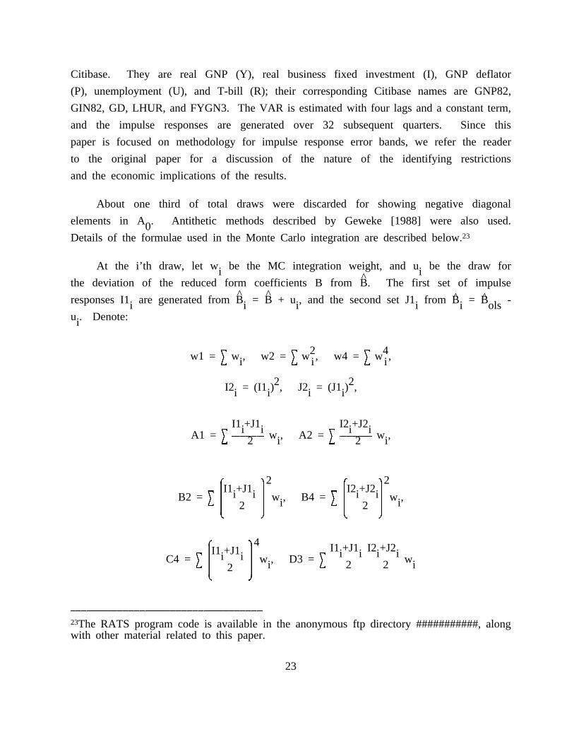
About one third of total draws were discarded for showing negative diagonal

elements in A . Antithetic methods described by Geweke [1988] were also used.023Details of the formulae used in the Monte Carlo integration are described below.

At the i’th draw, let w be the MC integration weight, and u be the draw fori i^the deviation of the reduced form coefficients B from B. The first set of impulse^ ^ ^ ^responses I1 are generated from B = B + u , and the second set J1 from B = B -i i i i i ols

u . Denote:i

s s 2 s 4w1 = w , w2 = w , w4 = w ,t i t i t i

2 2I2 = (I1 ) , J2 = (J1 ) ,i i i i

I1 +J1 I2 +J2s i i s i iA1 = ----------------------------- w , A2 = ----------------------------- w ,t 2 i t 2 i

( ) ( )2 22 2 2 2I1 +J1 I2 +J2s si i i iB2 = 2 2 w , B4 = 2 2 w ,----------------------------- -----------------------------t i t i2 22 2 2 29 0 9 0

( )42 2 I1 +J1 I2 +J2I1 +J1s s i i i ii iC4 = 2 2 w , D3 = ----------------------------- ----------------------------- w-----------------------------t i t 2 2 i22 29 0

---------------------------------------------------------------------------------------------------------------------------------------------------------------------------23The RATS program code is available in the anonymous ftp directory ###########, alongwith other material related to this paper.

23

2The mean of an impulse response is A1/w1 and the variance A2/w1 - (A1/w1) . The

variance of the Monte Carlo sampling error in the mean is

w2 ( 2 )------------------ B2/w1 - (A1/w1) .2 9 0w1

Finally, the estimated variance of the Monte Carlo error in the impulse response

variance is:

w2 ( 2 ) w4 ( 2 )------------------ B4/w1 - (A2/w1) + ------------------ C4/w1 - (B2/w1)2 9 0 4 9 0w1 w1

w2 ( 2 )- ------------- (D3/w1)(A1/w1) - (A2/w1)(A1/w1) .w1 9 0

Computation of the weighted Monte Carlo estimates of response bands shown in

Figure 4.1 took about 35 minutes on a 486/50 PC. There were 3000 draws, including

discards. The estimated means of the impulse responses have standard deviations of

Monte Carlo sampling error of 1-5% of the levels of the responses at their peaks, for

the most part. The estimated standard deviations of the responses have standard

deviations of Monte Carlo sampling error of about 12-20% of their estimated levels.

5. Conclusion

We have documented the difficulty in translating any bootstrap-style calculation

of small sample distribution theory for impulse responses into useful conclusions

about the shape of confidence intervals. We have shown that the already widely used

Bayesian methods behave reasonably and give an accurate picture of the effects of

nonlinearity and asymmetry in distributions of uncertainty about responses. We have

showed how to extend the widely used Bayesian procedures for just-identified models

correctly to over-identified models, displaying in an example the potential

importance to conclusions of carrying out these calculations correctly. Along the

way we have flagged some pitfalls that could catch, indeed already have caught, even

very astute practitioners.

24

REFERENCES

Blanchard, O.J. and D. Quah, 1989. "The Dynamic Effects of Aggregate Demand andSupply Disturbances,"American Economic Review 79, September, 655-73.

Box, G.E.P. and George Tiao, 1973. Bayesian Inference in Statistical Analysis,Addison-Wesley.

Chao, J. and P.C.B. Phillips, 1994. "Bayesian Model Selection in Partially Non-Stationary Vector Autoregressive Processes with Reduced Rank Structure," processed,Yale University.

Geweke, John, 1988. "Antithetic Acceleration of Monte Carlo Integration in BayesianInference,"Journal of Econometrics 38, 129-47.

Gordon, D.B. and E.M. Leeper, 1993. "The Dynamic Impacts of Monetary Policy: AnExercise in Tentative Identification,"Working Paper 93-5, Federal Reserve Bank ofAtlanta. To appear in theJournal of Political Economy.

Phillips, P.C.B., 1992. "To Criticize the Critics: An Objective Bayesian Analysis ofStochastic Trends,"Journal of Applied Econometrics.

Poterba, J.M., J.J. Rotemberg and L.H. Summers, 1986. "A Tax-Based Test for NominalRigidities," American Economic Review 76, September, 659-675.

Runkle, D.E., 1987. "Vector Autoregressions and Reality",Journal of Business andEconomics Statistics 5, October, 437-442.

----------------------------------------------, 1986. "Are Forecasting Models Usable for Policy Analysis?" FederalReserve Bank of MinneapolisQuarterly Review 10, 2-15.

Sims, C.A. and H. Uhlig, 1992. "Understanding Unit Rooters: A Helicopter Tour,"Econometrica.

25