Fachtagung “Lasermethoden in der Strömungsmesstechnik”4.–6. September 2012, Rostock

Erosion of a Strong Density Stratification by a Vertical Air Jet

Erosion einer Dichtestratifizierung durch einen vertikalen Luft Jet

R. Kapulla*, G. Mignot*, D. Paladino*

*Labor für Thermohydraulik (LTH), Paul Scherrer Institut, 5232 Villigen, Schweiz

Abstract

Computational Fluid Dynamics (CFD) codes are increasingly used for safety analysis tosimulate transient containment conditions after various severe accident scenarios in Nu-clear Power Plants (NPP). Consequently, the reliability of such codes must be benchmarkedagainst experimental data obtained in large scale facilities. Inspired, but not restricted tothese accident scenarios, a series of fundamental mixing experiments were performed inthe large scale PANDA test section built at the Paul Scherrer Institute in Switzerland, high-lighting the interaction of a vertical air jet emerging from a tube below a helium-rich airlayer. The isothermal experiments address the (i) the mechanisms of the gas transport andthe (ii) entrainment of the helium stratification located just beneath the vessel dome. Theexperiments were conducted under conditions characterized by an initially non-buoyantjet which becomes negatively buoyant and rapidly decelerates when it reaches the heliumstratification. For comparison purposes, additional experiments were performed for a pure,non-buoyant air jet emerging into the vessel in the absence of the helium stratification but,having the same exit velocity as the stratified case. For the stratified experiment it is shownthat the axial velocity v decays much faster already below the jet impingement zone com-pared with a corresponding free air jet while the turbulent kinetic energy remains on thesame level as for the free jet until it levels off once the stratification is reached.

1 Introduction

A jet of fluid with density which is directed into a volume of fluid of density with 6= ora jet () impinging onto a stable density stratification () is encountered in industry and at work.The sewage disposal through a pipe into a river or the sea is industrially widespread used to mix thewastewater with fresh water. For example, after the cooling of a power plant. Using an air conditionerfor the heating or cooling of a room, a jet of different temperature and therefore different density maybe forced into the room through a ceiling vent. Buoyant jets resulting from temperature and / or salinitydifferences can occur in the ocean and the atmosphere. An overview of the different phenomena and thephysics in buoyant turbulent jets can be found in [6, 1].A jet with the density is called positively buoyant when the jet fluid is injected vertically upwardsinto an ambient fluid with a higher density . The buoyancy force and the momentum have the samedirection and the buoyancy force adds to the momentum such that the velocity decay, common for non-buoyant jets is partly compensated and for strong buoyancy forces the jet might even accelerate. Whenthe buoyancy and the momentum forces have opposite directions the jet is called negatively buoyant, i.e.the negative buoyancy decelerates the jet much faster compared with a non-buoyant jet.The experiments presented in the paper describe the interaction of a vertical, upward projecting air jetemerging from a tube below a helium-rich air layer. The isothermal experiments address the (i) themechanisms of the gas transport and the (ii) entrainment of the helium stratification located just beneath

16 - 1

the vessel dome. The experiments were conducted under conditions characterized by a jet which isinitially non-buoyant and becomes negatively buoyant and decelerates when it reaches the helium strati-fication. Results depicting the mixing, transport and transient helium stratification erosion are presentedin terms of 2D PIV measurements which were used to measure the flow velocities at different locationsand in particular at the interface between the helium layer and the upward flowing jet. Additional gasconcentration profiles measured with a mass spectrometer are used to illustrate the erosion process ofthe density stratification. Initially, the vertical jet discharges into a neutral environment, i.e. = andtherefore has physical characteristics similar to a classical non-buoyant jet. After a certain distance, theambient density continuously decreases such that the non-buoyant jet becomes increasingly negativelybuoyant when penetrating the helium rich layer and the axial velocity decays very rapidly. Fluid accu-mulates in this mixing zone and a part of the fluid is flowing back in a small annulus around the upwardflow. By this transient mechanism, the helium layer is continuously eroded and helium is transportedinto lower parts of the test section such that the jet becomes increasingly negatively buoyant right fromthe beginning.In the next section we give a brief introduction of the experimental facility, the instrumentation and theexperimental parameters. For comparison purposes, we start presenting turbulence characteristics fora pure air jet emerging into the vessel in the absence of the helium stratification but, having the sameexit velocity as the stratified case. These results are compared with the literature. In the second partwe discuss the details of the erosion process in the presence of a helium rich stratification. Although acomplete experimental series was perform with varying initial jet velocities and different stratificationstrengths, we will focus the presentation on one unstratified and one stratified jet experiment.

2 Experiments

This section provides a brief overview of the facility, the instrumentation used for the experiments andthe experimental parameters. The experiments were performed in a vessel having an inner diameter of 4 and a height of 8, Figure 1. The air for the jet is injected through a tube at the axis of symmetry ofthe vessel. The injection tube has a 90 ◦ bend close to the bottom of the vessel. Since the straight tubepast the bend has a length of 15 it is expected that possible disturbances introduced by the bend areremoved by the turbulence due to the high tube Reynolds numberRe0 = 140000, Table 1. Consequently,

air

a) b)

injectiontube

injectiontube

> 15 dt

dt

air

v 0

v 0 ρ0,air ρ0,amb

ρ0,l

8 m

4 m∅

(0,0) x, u

y, vz, w

h

2 m

≈0

4 m

He-airinterface

He rich air layercamera

window

Pos A

Pos B

Pos C

Figure 1: Schematic of the experimental setup for the pure air jet a) and the air jet with helium rich airlayer in the vessel dome b).

16 - 2

-1000

0

1000

2000

3000

4000

0.8 1.0 1.2

b)

ρ0,air

ρ0,l

air jet injectionlevel

pure air

transitionzone, h

helium rich air layer

E_20, t = 0 s

ρ0 , kg/m

3

y,m

m

a)

instrumentationwires

helium rich air layer

hp

jet

Pos_B

1000 mm ≈

80

0 m

m

≈

Figure 2: Example PIV image recorded at position B showing the seeded jet from below, the non seededhelium rich air layer at the top and the horizontal instrumentation wires a). Initial density profilerecorded in the symmetry axis of the test section b).

the velocity profile at the tube exit are expected to show top hat characteristics with boundary layerstypical for turbulent pipe flows. In contrast to some past jet experiments where a smooth contractionnozzle at the tube exit was used to pronounce the top hat velocity profile by compressing the boundarylayers, we used an injection tube with a constant inner diameter of = 0075 . For a comparisonbetween the two types of initial velocity profiles for straight and contraction nozzles at the tube exit seeFig. 1 in [8] . The pressure was kept constant at 1 bar absolut by venting the vessel through a tubelocated at the bottom of the vessel.The tube exit is located 4 above the bottom of the test section to avoid any wall effects in the vicinityof the tube exit. The coordinate system origin to describe the experiments is located at the injectiontube exit and the light sheet for the PIV recordings coincides with the − plane, Figure 1. ThePIV camera was mounted in front of an upper vessel window on a translation stage consisting of twogoniometer and a rotation table. By vertically inclining the camera it was either possible to record threedifferent field-of-views (FOV) for the steady state jet experiments or to follow successively the erosionfront for the jet-layer experiments. The three FOV’s are depicted as Pos_A, Pos_B and Pos_C in Figure1 a). An example for a PIV image recorded at position B is shown in Figure 2 a). The image givesan impression of the jet-layer interaction zone. The seeded jet entering from below impinges onto thenon seeded helium rich layer and penetrates the stratification. Olive oil, dispersed into small dropletsby a spray nozzle, was used as seeding particles for the PIV technique. The oil particles were injectedinto the air injection tube that was directed into the vessel through the injection line. The PIV systemprovides 2D velocity fields with a typical acquisition rate of 5 . For the calculation of statisticalquantities 2048 image pairs were averaged. The PIV system consisted of a Quantel Twins B doublepulse laser with a maximum output energy of 380 and a double frame CCD camera type Imager ProX which is identical to the PCO.1600 camera, with a resolution of 1600x1200 pixel. The base analysiswas performed with DaVis 7.2 and the extended analysis with in house written MATLAB routines.For the base analysis consisting in the calculation of the instantaneous velocity vector maps, the imagebackground calculated as the mean of all the raw PIV images was subtracted and we applied a multi passanalysis with decreasing window sizes (128 → 64→ 32) where for each window size the velocity wascalculated with two passes. The velocity fields for interrogation window sizes of 128x128 and 64x64was calculated with 0 % overlap while we used 50 % overlap for the final size of 32x32 i.e. an effectivespatial resolution of 16x16. For the de-warping of the images, i.e. the translation of the raw pixelcoordinates to physical units and the removal of perspective distortions arising from the inclination of thecamera with respect to the calibration target, we used the DaVis built-in so called ’high accuracy mode’for the final pass of the velocity calculation which consists in a Whittaker reconstruction of the images.Although much more time consuming this was necessary to result in reliable velocity statistics, since thestandard reconstruction resulted for some (but not all) rms velocity fields in un-physical moire patterns.

16 - 3

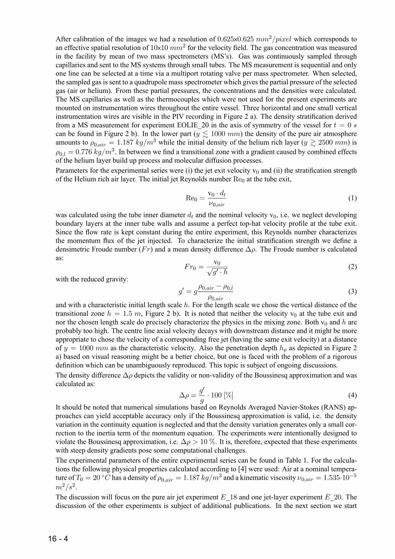
After calibration of the images we had a resolution of 0625x0625 2 which corresponds toan effective spatial resolution of 10x102 for the velocity field. The gas concentration was measuredin the facility by mean of two mass spectrometers (MS’s). Gas was continuously sampled throughcapillaries and sent to the MS systems through small tubes. The MS measurement is sequential and onlyone line can be selected at a time via a multiport rotating valve per mass spectrometer. When selected,the sampled gas is sent to a quadrupole mass spectrometer which gives the partial pressure of the selectedgas (air or helium). From these partial pressures, the concentrations and the densities were calculated.The MS capillaries as well as the thermocouples which were not used for the present experiments aremounted on instrumentation wires throughout the entire vessel. Three horizontal and one small verticalinstrumentation wires are visible in the PIV recording in Figure 2 a). The density stratification derivedfrom a MS measurement for experiment EOLIE_20 in the axis of symmetry of the vessel for = 0 can be found in Figure 2 b). In the lower part ( . 1000 ) the density of the pure air atmosphereamounts to 0 = 1187

3 while the initial density of the helium rich layer ( & 2500 ) is0 = 0776

3. In between we find a transitional zone with a gradient caused by combined effectsof the helium layer build up process and molecular diffusion processes.Parameters for the experimental series were (i) the jet exit velocity v0 and (ii) the stratification strengthof the Helium rich air layer. The initial jet Reynolds number Re0 at the tube exit,

Re0 =v0 · 0

(1)

was calculated using the tube inner diameter and the nominal velocity v0, i.e. we neglect developingboundary layers at the inner tube walls and assume a perfect top-hat velocity profile at the tube exit.Since the flow rate is kept constant during the entire experiment, this Reynolds number characterizesthe momentum flux of the jet injected. To characterize the initial stratification strength we define adensimetric Froude number () and a mean density difference ∆. The Froude number is calculatedas:

0 =v0√0 · (2)

with the reduced gravity:

0 = 0 − 0

0(3)

and with a characteristic initial length scale . For the length scale we chose the vertical distance of thetransitional zone = 15 , Figure 2 b). It is noted that neither the velocity v0 at the tube exit andnor the chosen length scale do precisely characterize the physics in the mixing zone. Both v0 and areprobably too high. The centre line axial velocity decays with downstream distance and it might be moreappropriate to chose the velocity of a corresponding free jet (having the same exit velocity) at a distanceof = 1000 as the characteristic velocity. Also the penetration depth as depicted in Figure 2a) based on visual reasoning might be a better choice, but one is faced with the problem of a rigorousdefinition which can be unambiguously reproduced. This topic is subject of ongoing discussions.The density difference∆ depicts the validity or non-validity of the Boussinesq approximation and wascalculated as:

∆ =0

· 100 [%] (4)

It should be noted that numerical simulations based on Reynolds Averaged Navier-Stokes (RANS) ap-proaches can yield acceptable accuracy only if the Boussinesq approximation is valid, i.e. the densityvariation in the continuity equation is neglected and that the density variation generates only a small cor-rection to the inertia term of the momentum equation. The experiments were intentionally designed toviolate the Boussinesq approximation, i.e. ∆ 10 %. It is, therefore, expected that these experimentswith steep density gradients pose some computational challenges.The experimental parameters of the entire experimental series can be found in Table 1. For the calcula-tions the following physical properties calculated according to [4] were used: Air at a nominal tempera-ture of 0 = 20 ◦ has a density of 0 = 1187

3 and a kinematic viscosity 0 = 1535·10−522.The discussion will focus on the pure air jet experiment _18 and one jet-layer experiment _20. Thediscussion of the other experiments is subject of additional publications. In the next section we start

16 - 4

comparing the turbulence characteristics of the pure air jet with the literature. This is followed bycomparing the findings for the pure air jet with the jet-layer experiment.

Exp. Type ̇ v0 Re0 0 0 ∆ − % 3 − %

E_18 pure jet 15 286 140000 0 − −_21 pure jet 28 533 260000 0 − −

E_20 jet & layer 15 286 140000 40 0776 127 347_22 jet & layer 15 286 140000 25 0930 160 217

_23 jet & layer 28 533 260000 40 0776 236 347_19 jet & layer 28 533 260000 25 0930 298 217_24 jet & layer 28 533 260000 25 0930 298 217

Table 1: Main nominal parameters for the different experiments.

3 Results

x [mm]

y[m

m]

-400 -200 0 200 400

1000

1500

2000

2500

v: 0 0.1 0.2 0.3 0.4 0.5 0.6 0.7 0.8 0.9 1 1.1 1.2

Figure 3: Downstream development of the axial ve-locity during the pure air jet experiment _18.

Pure air jet experiments. The downstream de-velopment of the axial velocity (v) of the pureair jet experiment (_18) is presented in Figure3 as a color coded map where stream lines wereadded. After a linear interpolation of the results toa common grid having a size of 110x220, the threesuccesively recorded FOV’s, Figure 1 a), were‘stitched’ together making use of the steady stateassumption. The resulting FOV covers a rangeof ≈ 09x20 2. Except for the weak off-axisdisplacement far downstream ( 2000 )we find a velocity map distribution as expectedand described in the literature [7, 6, 5]. The ax-ial velocity profiles can be presented in self simi-lar coordinates. The necessary local characteristiclength scale – the half-width radius 05 – and thelocal characteristic velocity scale – the maximumvelocity v – can be derived from applying theGaussian fit function

v() = v + v · exp(− ln(2)

µ−

05

¶2)(5)

to the axial velocity profiles. The horizontal dis-placement of the velocity is depicted by and apossible velocity offset outside the the jet by v.Since v ≈ 0 this term is not considered fur-ther. Here and in the following we denote timeaverages with an overbar and fluctuating quanti-ties with a prime according to the common ve-locity decomposition v() = v+v0(). The axialvelocity profiles can thus be presented in similar-

16 - 5

ity coordinates = ( − )05 and v()v. An example of an axial velocity profile extracted at = 1440 from Figure 3 with the corresponding Gaussian fit function according to Eq. 5 is shownin Figure 4 a). Next, the axial velocity profiles were extracted for each coordinate on the common grid110x220 which results in 220 velocity profiles ∈ [900 2900] and Eq. 5 was applied to each ofthe profiles by a least square method. From the 220 velocity profiles, we present 11 in non-dimensionalform in Figure 4 b).

-400 -200 0 200 4000.0

0.2

0.4

0.6

0.8

1.0

a)

y = 1440 mm Gaussian fit

v , m

m

x , mm

-2 -1 0 1 20.0

0.2

0.4

0.6

0.8

1.0

b)

y [900 2000] mm

v / v

c , -

η = (x-xc ) / r

0.5 , -

-2 -1 0 1 20.0

0.2

0.4

0.6

0.8

1.0

c)

interpolated to regular η grid

η = (x-xc ) / r

0.5 , -

v / v

c , -

-2 -1 0 1 20.0

0.2

0.4

0.6

0.8

1.0

EOLIE_18 Hussein et al. (1994)

d)

η = (x-xc ) / r

0.5 , -

< v

/ vc >

, -

Figure 4: Normalization and spatially averaging process of thenon-dimensional axial velocity profiles for experiment _18.Mean velocity profile v() with Gaussian fit at = 1400 a), non-dimensional presentation of 11 downstream velocity pro-files b), the same profiles as in b) but with an interpolation to aregular grid for c) and spatially averaged non-diemsnional ax-ial velocity profile with error margins and comparison with theliterature d).

To calculate a final representa-tive non-dimensional velocity pro-file, the individual profiles were lin-early interpolated to a regular non-dimensional coordinate grid, Fig-ure 4 c), and finally all of the 220profiles were spatially averaged, Fig-ure 4 d),

hv()i = 1

v()

X

v() (6)

with v() = 220 for velocitiesclose to the tube axis and accord-ingly smaller further away from theaxis. Here and subsequently we de-note spatial averages with the nota-tion hi. From the the standard de-viation of the averaging:

hv()i =s1

v−1X

{hv()i− v()}2

(7)we calculated the errors of the meannon-dimensional spatially averagedvelocity hv()i according:

hv()i = · hv()ip()

(8)

where depicts the 99 % two sidedconfidence interval taken from theStudent’s t-distribution for of a sys-tem with degrees of freedom.

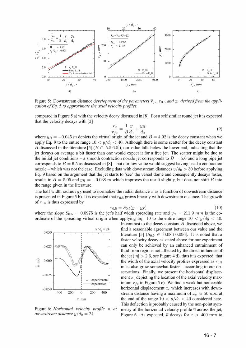
The effective number of samples () used for the error calculation is by a factor of 10 smaller com-pared with v() because adjacent velocity profiles are not statistically independent. Calculating theintegral length scale v in direction from the integration of the spatial cross-correlation function of thevelocity signal v() reveals that approximately every 22 velocity profile on the chosen grid (110x220)which corresponds to ∆ ≈ 100 is statistically independent. The results of the corresponding cal-culations are not presented here. The calculated errors hv()i are depicted in Figure 4 d) by error bars.Comparing our experimental results with previous measurements [2, 7], we find an excellent agreementfor the right half of the profile ( 0) while on the left side there is some lack of coincidence for −1which is caused by the weak horizontal deflection of the jet for large downstream distances discussedbelow.To further characterize the evolving jet, the development of the parameters v, 05 and as derivedfrom the application of Eq. 5 to the axial velocity profiles are presented in Figure 5 for normalized down-stream distances 10 0 40. Only every 4 measurement point is displayed. The downstreamdevelopment of the normalized maximum axial velocities as obtained from the Gaussian fit v0v is

16 - 6

10 20 30 400.0

2.0

4.0

6.0

8.0

750 1500 2250 30000

100

200

10 20 30 40

0 20 40 600

1000

2000

30000 B

fc 0 0

yv 1 y

B d dv= ⋅ +

a)

B = 4.92y

B /d

0 = -0.608

vfc E_18

Fit to E_18 Xu & Antonia (B = 5.6)

y _

v 0 / v fc

, -

y / d0 , -

y / d0 , -

b)

S0.5

= 0.0975y

s = 211.9

0.5 0.5 sr S (y y )= ⋅ −

E_18 Fit to E_18

r 0.5 ,

mm

y , mm

c)

E_18 Fit to E_18

y , m

m

xc , mm

Figure 5: Downstream distance development of the parameters v, 05 and derived from the appli-cation of Eq. 5 to approximate the axial velocity profiles.

compared in Figure 5 a) with the velocity decay discussed in [8]. For a self similar round jet it is expectedthat the velocity decays with [2]

v0v

=1

0+

0(9)

where = −0045 depicts the virtual origin of the jet and = 492 is the decay constant when weapply Eq. 9 to the entire range 10 0 40. Although there is some scatter for the decay constant discussed in the literature [5] ( ∈ [55 65]), our value falls below the lower end, indicating that thejet decays on average a bit faster than one would expect it for a free jet. The scatter might be due tothe initial jet conditions – a smooth contraction nozzle jet corresponds to = 56 and a long pipe jetcorresponds to = 65 as discussed in [8] – but our low value would suggest having used a contractionnozzle – which was not the case. Excluding data with downstream distances 0 30 before applyingEq. 9 based on the argument that the jet starts to ’see’ the vessel dome and consequently decays faster,results in = 505 and = −0038 which improves the result slightly, but does not shift intothe range given in the literature.The half width radius 05 used to normalize the radial distance as a function of downstream distanceis presented in Figure 5 b). It is expected that 05 grows linearly with downstream distance. The growthof 05 is thus expressed by

05 = 05( − ) (10)where the slope 05 = 00975 is the jet’s half width spreading rate and = 2119 is the co-ordinate of the spreading virtual origin when applying Eq. 10 to the entire range 10 0 40.

-400 -200 0 200 400-0.050

-0.025

0.000

0.025

0.050

experimantal expectation

y / d0 = 24

u, m

/s

x, mm

Figure 6: Horizontal velocity profile atdownstream distance 0 = 24.

In contrast to the decay constant discussed above, wefind a reasonable agreement between our value and theliterature [5] (05 ∈ [0086 0096]. It is noted that afaster velocity decay as stated above for our experimentcan only be achieved by an enhanced entrainment offluid from regions not affected by the direct influence ofthe jet (|| 26, see Figure 4 d), thus it is expected, thatthe width of the axial velocity profiles expressed as 05must also grow somewhat faster – according to our ob-servations. Finally, we present the horizontal displace-ment depicting the location of the axial velocity max-imum v in Figure 5 c). We find a weak but noticeablehorizontal displacement which increases with down-stream distance having a maximum of ≈ 50 atthe end of the range 10 0 40 considered here.This deflection is probably caused by the non-point sym-metry of the horizontal velocity profile across the jet,Figure 6. As expected, decays for 400 to

16 - 7

almost zero, but for −300 we find a persistent velocity of ≈ 25 projecting towards thejet axis instead of the expected decay to zero. We find similar non-point symmetric horizontal velocityprofile shapes for any downstream distance. This weak horizontal velocity projecting towards the jet axismost probably causes the jet deflection (Figure 5 c) as well as the asymmetry of the non-dimensionalaxial velocity profile (Figure 4 d) by hindering the jet expansion into the outer mixing zone ( −1) oreven by compressing this zone.Air jet impinging onto a helium rich air layer. For the helium rich air layer build-up we injected heliumfor a certain amount of time determined in scoping tests through a tube close to the vessel dome untilthe desired helium concentration is reached. The initial density profile for experiment _20 (see alsoTable 1) measured at the symmetry axis of the test section is shown in Figure 2 b). In the lower part ofthe vessel we have initially an air atmosphere at room temperature (0 ≈ 20 ◦) while the helium-airmixture with a lower density is trapped in the vessel dome. For details on the helium filling proceduresee [3]. The measurement is initiated by opening a valve to release the air jet ( = 0 ) and the entireexperiment is finished when the helium rich layer is completely eroded such that we measure similardensities in the entire vessel ( ' 190000 ). Typical mean axial velocity v and turbulent kinetic energy maps measured in the air jet impinging onto the helium rich air layer from below are shown in Figure 7right after the beginning of the jet injection 1 = [53 463] and after the erosion process has proceededsome time 2 = [4590 5000] . Consequently, it was necessary to move the FOV from PosA to PosB tofollow the erosion process (Figure 1 a). The kinetic energy was calculated by

=1

2

n(v0)2 + 2 · (0)2

o(11)

with (v0)2 and (0)2 depicting the variance of the velocity fluctuations in and direction, respectively.Due to its momentum, the jet continuously penetrates upwards into the helium rich layer. Through

x [mm]

y[m

m]

-400 -200 0 200 4001600

1800

2000

2200

v0.60.5250.450.3750.30.2250.150.0750

-0.075-0.15

m/s

c)

S03_PosB

t 2= [4590 5000] sx [mm]

y[m

m]

-400 -200 0 200 4001600

1800

2000

2200

k0.050.040.030.020.010

m2/s2

d)

S03_PosB

t 2= [4590 5000] s

x [mm]

y[m

m]

-400 -200 0 200 400

1000

1200

1400

1600

v

10.90.80.70.60.50.40.30.20.10

-0.1-0.2m/s

a)

S01_PosA

t 1= [53 463] sx [mm]

y[m

m]

-400 -200 0 200 400

1000

1200

1400

1600

k0.10.080.060.040.020

m2/s2

b)

S01_PosA

t 1= [53 463] s

Figure 7: Mean axial velocity v ( a and c) and turbulent kinetic energy maps (b and d) measured inthe air jet impinging onto the helium rich air layer for 1 = [53 463] and 2 = [4590 5000] whichcorresponds to position A and B in Figure 1 a).

16 - 8

the action of the negative buoyancy, the axial velocity experiences a strong deceleration in the vicinityof the helium rich layer (the mixing zone), Figure 7 a) and c) and the jet is finally stopped within adistance of ≈ 500 . Fluid accumulates in a continuous process in this mixing zone and part of thefluid consisting now in an air helium mixture is flowing back in an annular region around the upwardflowing jet as indicated by the streamlines. Consequently, the jet decelerates additionally, because thedownwards annular flow slows down the upward jet flow. At least for the initial stage of the erosionprocess, Figure 7 a), the outwards spreading streamlines seems to indicate that the outward flow is notpassing all the way down to the jet orifice and eventually even further down to the vessel bottom, butdown to a level where the density of the annular flow equals the density of the helium stratificationsuch that the fluid starts to spread radially. The main difference between the early stage of the erosionprocess (1) and a later time (2), is the stronger confinement of the flow around the jet for 1, Figure 7a) versus c), which can directly be attributed to the spreading through entrainment of ambient fluidof the (free) jet with downstream distance, Figure 5 b). The latter observation equally applies to theturbulent kinetic energy map Figure 7 b) versus d). While we initially find ≈ 01 22 in the jetcore (1), the kinetic energy is later distributed to a larger area such that we find ≈ 004 22 (2).This finding is detailed in the next figure. The axial velocity and the kinetic energy decay in the jetimpingement zone are compared in Figure 8 by means of vertical line profiles extracted at = 0

with the corresponding values from the free jet experiment (_18) together with corresponding densityprofiles for 1 = [53 463] and 2 = [4590 5000] . Due to the higher momentum of the jet at 1, wefind the axial velocity v decays to v ≈ 0 beyond the level ≈ 1400, where the density startsdecreasing and accordingly, the turbulent kinetic energy approaches ≈ 022 also beyond this level,Figure 8 a, b and c. It is also shown that v decays much faster below and in the jet impingement zonecompared with a corresponding free air jet while remains on the same level as for the free jet until itlevels off. Later in time (2), the decay of v to zero coincides almost with the beginning of the heliumstratification, i.e. where decreases, as does the decay of .

1600

1800

2000

2200

2400

0.0 0.4 0.8

1000

1200

1400

1600

1800

2000

0.0 0.4 0.8 1.2

EOLIE_20 (jet & helium) fit

___________

EOLIE_18 (pure air jet) fit

d)

v , m/s

y, m

m

0.00 0.04

e)

k, m2 / s2

0.8 1.0 1.2

f)

t2 = [4590 5000] s

S03_PosB

ρ , kg/m3

EOLIE_20 (jet & helium) fit

___________

EOLIE_18 (pure air jet) fit

a)

v , m/s

y, m

m

0.00 0.04 0.08

b)

k, m2 / s2

0.8 1.0 1.2

c)

t1 = [53 463] s

S01_PosA

ρ , kg/m3

Figure 8: Vertical line profiles of the mean axial velocity decay v ( a and d), turbulent kinetic energy decay (b and d) and density profiles (c and f) measured in the mixing zone for = [53 463] and = [4590 5000] . The results for v and are compared with corresponding measurements for the freeair jet (_18).

16 - 9

4 Conclusions and Outlook

A series of fundamental mixing experiments was presented, highlighting the interaction of a vertical airjet emerging from a tube below a helium rich air layer. These experiments were performed in one ofthe vessels in the large scale PANDA facility having a diameter of 4 and a height of 8 located atthe Paul Scherrer Institute in Switzerland. Although the vertical jet discharges initially into an neutralenvironment, the physical characteristics differ from a classical non-buoyant jet. It was shown that thevelocity decays faster already below the helium rich layer compared with the non-buoyant jet. Aftera certain distance, the ambient density continuously decreases such that the non-buoyant jet becomesincreasingly negatively buoyant when penetrating the helium rich layer and the axial velocity decays veryrapidly. Fluid accumulates in this mixing zone and a part of the fluid is flowing back in a small annulusaround the upward flow. By this transient mechanism, the helium layer is continuously eroded andhelium is transported into lower parts of the test section such that the jet becomes increasingly negativelybuoyant right from the beginning. For comparison purposes, additional experiments were performed fora pure, non-buoyant air jet emerging into the vessel in the absence of the helium stratification but, havingthe same exit velocity as the stratified case.From the non-dimensional presentation of the axial velocity v an excellent agreement of the right halfof the profile was found when compared with the literature, while the left side shows some lack ofcoincidence. This was most probably caused by a non-point symmetric profile of the horizontal velocity with a small non-vanishing horizontal velocity component outside the jet which causes a maximumjet deflection of ≈ 50 as well as the asymmetry of the non-dimensional axial velocity profile byhindering the jet expansion into the outer mixing zone. The calculated maximum axial velocity decayof the pure jet was faster than corresponding values in the literature and the jet spreading rate defined bythe half width radius 05 at the upper bound of other experiments.Due to the higher momentum it was found that the jet penetrates initially much deeper into the heliumrich stratification compared with later instances in time. Initially, the axial velocity v decays to v ≈ 0 beyond the level where the density starts decreasing and accordingly, the turbulent kinetic energyapproaches ≈ 022 also beyond this level. It was also shown that v decays much faster below andin the jet impingement zone compared with a corresponding free air jet while remains on the samelevel as for the free jet until it levels off. Later in time, the decay of v to zero coincides almost with thebeginning of the helium stratification, i.e. where decreases, as does the decay of .The other experiments will be analyzed in a similar manner and the ultimate goal is a non-dimensionalpresentation of the erosion speed as a function of jet momentum and stratification strength.

References

[1] C.-J. Chen and W. Rodi. Vertical turbulent buoyant jets: A review of experimental data. NASASTI/Recon Technical Report A, 80:23073–+, 1980.

[2] H. J. Hussein, S. P. Capp, and W. K. George. Velocity measurements in a high-reynolds-number,momentum-conserving, axisymmetric, turbulent jet. Journal of Fluid Mechanics, 258:31–75, 1994.

[3] R. Kapulla, D. Paladino, G. Mignot, R. Zboray, and S. Gupta. Break-up of gas stratification in LWRcontainment induced by negatively buoyant jets and plumes. In 17th International Conference onNuclear Engineering, volume 2009, pages 657–666. ASME, 2009.

[4] E. Lemmon, M. Huber, and M. McLinden. NIST Standard Reference Database 23: Reference FluidThermodynamic and Transport Properties-REFPROP, Version 9.0. National Institute of Standardsand Technology, Standard Reference Data Program, 2010.

[5] G. Lipari and P. Stansby. Review of experimental data on incompressible turbulent round jets.Applied Scientific Research, 87(1):79–114, 2011.

[6] E. List. Turbulent jets and plumes. Annual Review of Fluid Mechanics, 14:189–212, 1982.

[7] S. B. Pope. Turbulent flows. Cambridge University Press, 2000.

[8] Xu and Antonia. Effect of different initial conditions on a turbulent round free jet. Experiments inFluids, 33:677–683, 2002. 10.1007/s00348-002-0523-7.

16 - 10