erhic: electron beam polarization in the storage ring
TRANSCRIPT

1/27 P�i?��≫≪><
eRHIC: Electron Beam Polarization
in the Storage Ring
Outline
• Radiative polarization and the eRHIC storage ring.
• Simulations of polarization in the eRHIC storage ring.
– Effect of mis-alignments.
• Summary and Outlook.
Eliana GIANFELICE (Fermilab)EIC Meeting, JLab October 31, 2018

2/27 P�i?��≫≪><
Radiative polarization and the eRHIC storage ring
Experiments require
• Large proton and electron polarization (& 70%)
• Longitudinal polarization at the IP with
both helicities within the same store
• Energy
– protons: between 41 and 275 GeV
– electrons: between 5 and 18 GeV
e p
High proton polarization is already routinely achieved in RHIC.
Studies are needed instead for the electron beam polarization.
3/27 P�i?��≫≪><
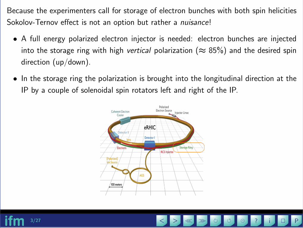
Because the experimenters call for storage of electron bunches with both spin helicities
Sokolov-Ternov effect is not an option but rather a nuisance!
• A full energy polarized electron injector is needed: electron bunches are injected
into the storage ring with high vertical polarization (≈ 85%) and the desired spin
direction (up/down).
• In the storage ring the polarization is brought into the longitudinal direction at the
IP by a couple of solenoidal spin rotators left and right of the IP.
� �

4/27 P�i?��≫≪><
In the eRHIC energy range the minimum
polarization time nominally is τp ' 30’
at 18 GeV. At first sight a large time
before Sokolov-Ternov effect reverses the
polarization of the down-polarized electron
bunches...
However the machine imperfections may quickly depolarize the whole beam.
5/27 P�i?��≫≪><
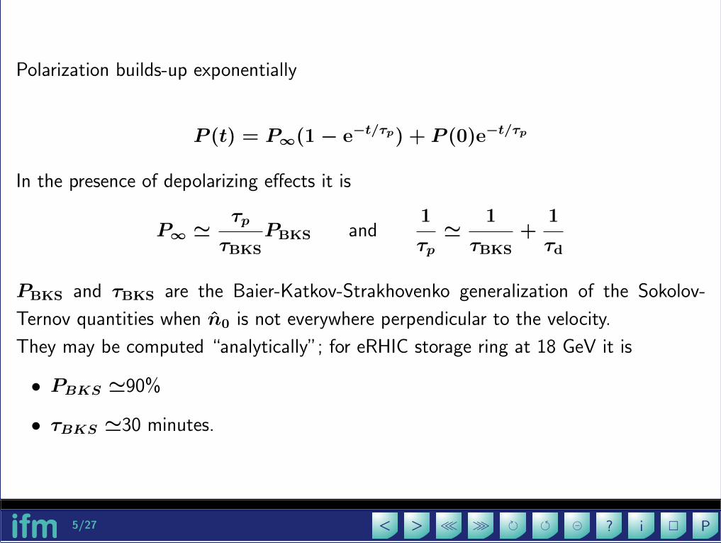
Polarization builds-up exponentially
P (t) = P∞(1− e−t/τp) + P (0)e−t/τp
In the presence of depolarizing effects it is
P∞ 'τp
τBKS
PBKS and1
τp'
1
τBKS
+1
τd
PBKS and τBKS are the Baier-Katkov-Strakhovenko generalization of the Sokolov-
Ternov quantities when n0 is not everywhere perpendicular to the velocity.
They may be computed “analytically”; for eRHIC storage ring at 18 GeV it is
• PBKS '90%
• τBKS '30 minutes.
6/27 P�i?��≫≪><
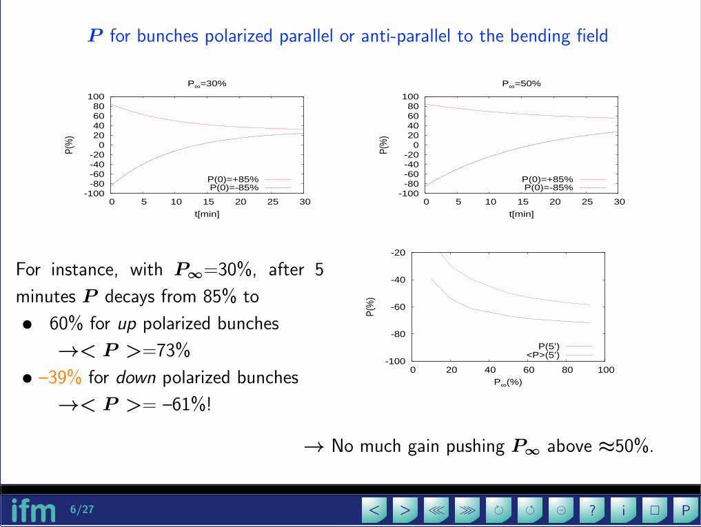
P for bunches polarized parallel or anti-parallel to the bending field
-100-80-60-40-20
0 20 40 60 80
100
0 5 10 15 20 25 30
P(%
)
t[min]
P∞=30%
P(0)=+85%P(0)=-85%
-100-80-60-40-20
0 20 40 60 80
100
0 5 10 15 20 25 30
P(%
)
t[min]
P∞=50%
P(0)=+85%P(0)=-85%
For instance, with P∞=30%, after 5
minutes P decays from 85% to
• 60% for up polarized bunches
→< P >=73%
• –39% for down polarized bunches
→< P >= –61%!
-100
-80
-60
-40
-20
0 20 40 60 80 100P(
%)
P∞(%)
P(5’)<P>(5’)
→ No much gain pushing P∞ above ≈50%.
7/27 P�i?��≫≪><
Simulations for the eRHIC storage ring
• Energy: 18 GeV, the most challenging.
• Simulations shown here are for the “ATS” optics with
– 900 FODO for both planes;
– β∗x=0.7 m and β∗y= 9 cm.
• Working point for luminosity: Qx=60.12, Qy=56.10, Qs=0.046
Tools:
• MAD-X used for simulating quadrupole misalignments and orbit correction.
• SITROS (by J. Kewisch) used for computing the resulting polarization.
– Tracking code with 2nd order orbit description and fully non-linear spin motion.
– Used for HERA-e in the version improved by M. Boge and M. Berglund.
– It contains SITF (6D) for analytical polarization computation with linearized
spin motion.
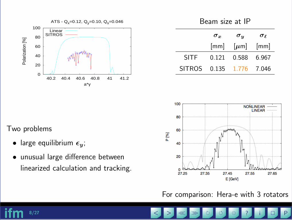
8/27 P�i?��≫≪><
0
20
40
60
80
100
40.2 40.4 40.6 40.8 41 41.2
Pola
rizat
ion
[%]
a*γ
ATS - Qx=0.12, Qy=0.10, Qs=0.046
LinearSITROS
Beam size at IP
σx σy σ`
[mm] [µm] [mm]
SITF 0.121 0.588 6.967
SITROS 0.135 1.776 7.046
Two problems
• large equilibrium εy;
• unusual large difference between
linearized calculation and tracking.
For comparison: Hera-e with 3 rotators

9/27 P�i?��≫≪><
Bmad (by D. Sagan) implemented on a MAC laptop for cross-checking SITROS re-
sults. 300 particles tracked over 6000 turns (typical SITROS parameters) with SR and
stochastic emission with Bmad “standard” tracking.
100
110
120
130
140
150
160
170
180
0 1000 2000 3000 4000 5000 6000
σ x[µ
m]
Turn #
0
10
20
30
40
50
60
70
80
90
100
0 1000 2000 3000 4000 5000 6000σ y
[µm
]Turn #
4000
6000
8000
10000
12000
14000
16000
18000
0 1000 2000 3000 4000 5000 6000
σ z[m
m]
Turn #
Beam size
σx σy σ` σE
[µm] [µm] [mm] [%]
analytical (Bmad) 123 0.4 7.0 0.1
Bmad tracking 120 2.0 6.7 0.1
SITROS 136 1.8 7.0 0.1
The large εy is not a SITROS artifact.
10/27 P�i?��≫≪><
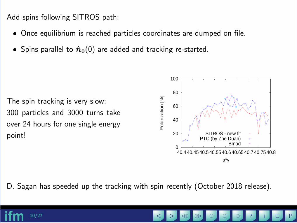
Add spins following SITROS path:
• Once equilibrium is reached particles coordinates are dumped on file.
• Spins parallel to n0(0) are added and tracking re-started.
The spin tracking is very slow:
300 particles and 3000 turns take
over 24 hours for one single energy
point!
0
20
40
60
80
100
40.4 40.45 40.5 40.55 40.6 40.65 40.7 40.75 40.8
Po
lariza
tion
[%
]a*γ
SITROS - new fitPTC (by Zhe Duan)
Bmad
D. Sagan has speeded up the tracking with spin recently (October 2018 release).
11/27 P�i?��≫≪><
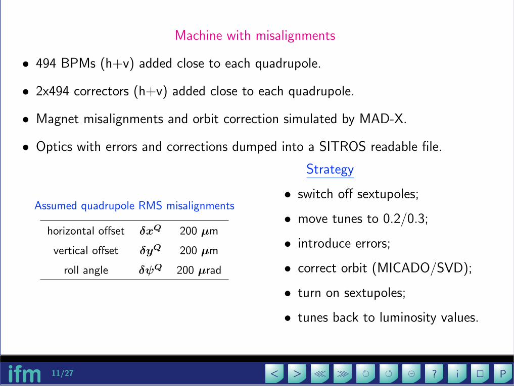
Machine with misalignments
• 494 BPMs (h+v) added close to each quadrupole.
• 2x494 correctors (h+v) added close to each quadrupole.
• Magnet misalignments and orbit correction simulated by MAD-X.
• Optics with errors and corrections dumped into a SITROS readable file.
Assumed quadrupole RMS misalignments
horizontal offset δxQ 200 µm
vertical offset δyQ 200 µm
roll angle δψQ 200 µrad
Strategy
• switch off sextupoles;
• move tunes to 0.2/0.3;
• introduce errors;
• correct orbit (MICADO/SVD);
• turn on sextupoles;
• tunes back to luminosity values.

12/27 P�i?��≫≪><
MAD-X fails correcting the orbit!
Example with only δyQ 6= 0 and sexts off.
Large discrepancy between what the correc-
tion module promises...
�� ��
...and the actual result!
-10
-5
0
5
10
15
0 500 1000
1500 2000
2500 3000
3500
y [mm
]
s [m]
BPMs
-20
-15
-10
-5
0
5
10
15
20
25
0 500 1000
1500 2000
2500 3000
3500
x [mm
]
s [m]
BPMs
↑Effect on horizontal plane
with sextupoles off
Separate horizontal and vertical orbit correction inadequate in the rotator sections
→ “external” program used for correcting horizontal and vertical orbits simultaneously.

13/27 P�i?��≫≪><
One error realization
• after orbit correction
• with Qx=60.10, Qy=56.20 (HERA-e tunes).
0
20
40
60
80
100
40.2 40.4 40.6 40.8 41 41.2 41.4
Pol
ariz
atio
n [%
]
a*γ
SITF - .1/.2/.046
PPxPyPs 0
5
10
15
20
25
30
35
40
40.2 40.4 40.6 40.8 41 41.2 41.4|δ
n|rm
s (m
rad)
a*γ
SITF - .1/.2/.046
14/27 P�i?��≫≪><
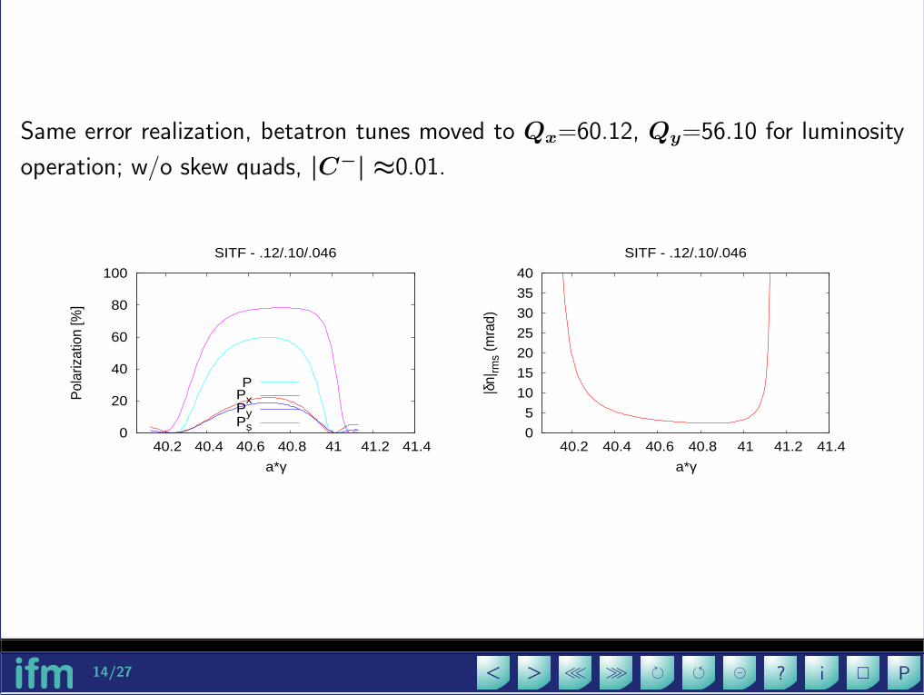
Same error realization, betatron tunes moved to Qx=60.12, Qy=56.10 for luminosity
operation; w/o skew quads, |C−| ≈0.01.
0
20
40
60
80
100
40.2 40.4 40.6 40.8 41 41.2 41.4
Pol
ariz
atio
n [%
]
a*γ
SITF - .12/.10/.046
PPxPyPs 0
5
10
15
20
25
30
35
40
40.2 40.4 40.6 40.8 41 41.2 41.4
|δn|
rms
(mra
d)
a*γ
SITF - .12/.10/.046
15/27 P�i?��≫≪><
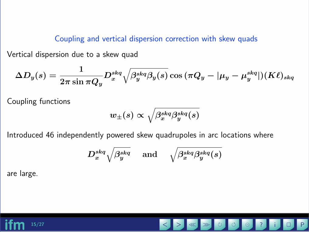
Coupling and vertical dispersion correction with skew quads
Vertical dispersion due to a skew quad
∆Dy(s) =1
2π sinπQy
Dskqx
√βskqy βy(s) cos (πQy − |µy − µskqy |)(K`)skq
Coupling functions
w±(s) ∝√βskqx βskqy (s)
Introduced 46 independently powered skew quadrupoles in arc locations where
Dskqx
√βskqy and
√βskqx βskqy (s)
are large.

16/27 P�i?��≫≪><
Same error realization, luminosity betatron tunes with optimized skew quads,
|C−| ≈0.002.
0
20
40
60
80
100
40.2 40.4 40.6 40.8 41 41.2 41.4
Pola
rizat
ion
[%]
a*γ
SITF - .12/.10/.046
PPxPyPs 0
5
10
15
20
25
30
35
40
40.2 40.4 40.6 40.8 41 41.2 41.4
|δn| rm
s (m
rad)
a*γ
SITF - .12/.10/.046
0
20
40
60
80
100
40.2 40.4 40.6 40.8 41 41.2 41.4
Pola
rizat
ion
[%]
a*γ
ATS - Qx=0.12, Qy=0.10, Qs=0.046
LinearSITROS
Beam size at IP
σx σy σ`
[mm] [µm] [mm]
SITF 0.121 1.718 6.984
SITROS 0.138 3.126 6.969
17/27 P�i?��≫≪><
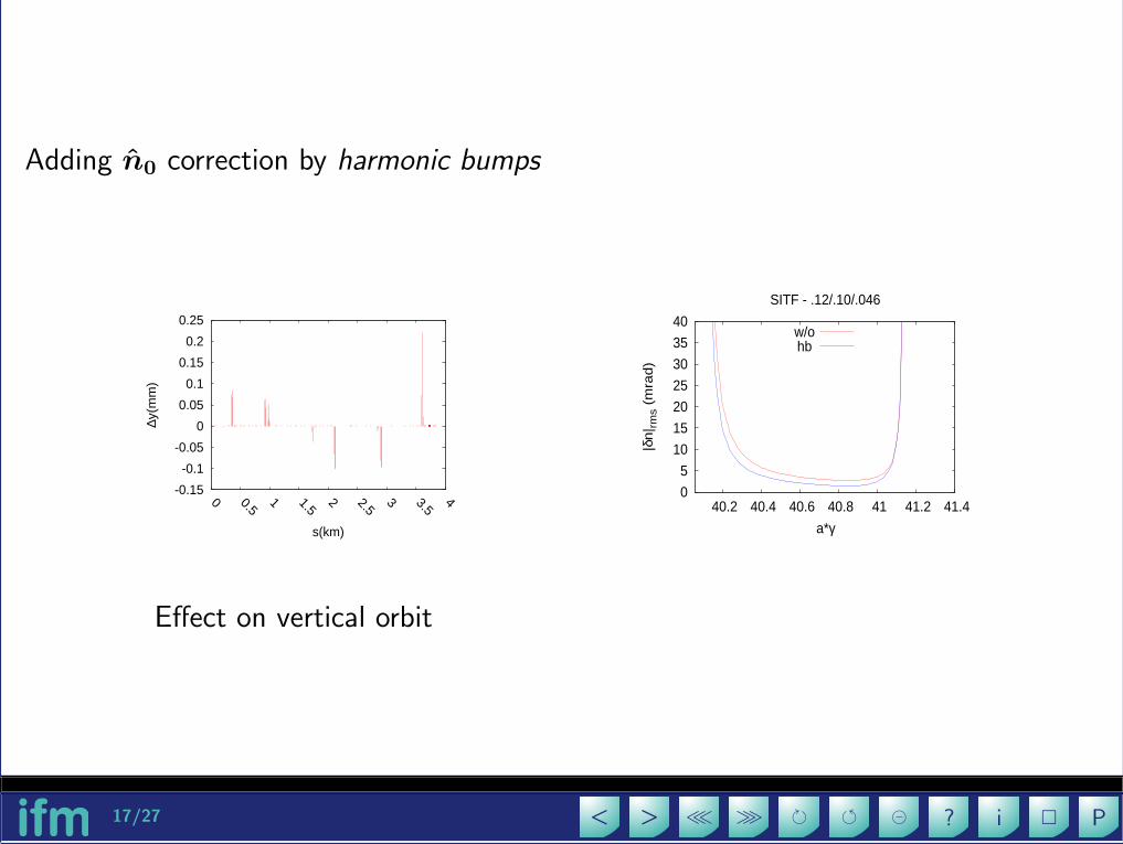
Adding n0 correction by harmonic bumps
-0.15
-0.1
-0.05
0
0.05
0.1
0.15
0.2
0.25
0 0.5 1 1.5
2 2.5 3 3.5
4
∆y(m
m)
s(km)
Effect on vertical orbit
0
5
10
15
20
25
30
35
40
40.2 40.4 40.6 40.8 41 41.2 41.4
|δn| rm
s (m
rad)
a*γ
SITF - .12/.10/.046
w/ohb

18/27 P�i?��≫≪><
0
20
40
60
80
100
40.2 40.4 40.6 40.8 41 41.2 41.4
Pol
ariz
atio
n [%
]
a*γ
SITF - .12/.10/.046
PPxPyPs
Beam size at IP
σx σy σ`
[mm] [µm] [mm]
SITF 0.121 3.151 6.985
SITROS 0.139 4.402 7.004
0
20
40
60
80
100
40.2 40.4 40.6 40.8 41 41.2 41.4
Pol
ariz
atio
n [%
]
a*γ
ATS - Qx=0.12, Qy=0.10, Qs=0.046
LinearSITROS
0
10
20
30
40
50
60
40.4 40.45 40.5 40.55 40.6 40.65 40.7 40.75 40.8
Pol
ariz
atio
n [%
]
a*γ
ATS - Qx=0.12, Qy=0.10, Qs=0.046
unpert.pert.
Level of polarizations is as for the unper-
turbed optics. However: BPMs errors must
be included and some statistics is needed!

19/27 P�i?��≫≪><
εy bump
The beam vertical emittance is 1.7 pm, corresponding to σ∗y ' 0.4 µm. A larger beam
size at the IP may be needed.
The e-beam εy may be efficiently increased by anti-symmetric bumps around low βy
locations.
As a test such a bump has been introduced around the IP.
Effect on polarization is detrimental. For εy= 3 nm there is no polarization!
0
20
40
60
80
100
40 40.2 40.4 40.6 40.8 41 41.2 41.4
Pol
ariz
atio
n [%
]
a*γ
ATS - Qx=0.12, Qy=0.10, Qs=0.046
PPxPyPs 0
2
4
6
8
10
40 40.2 40.4 40.6 40.8 41P
olar
izat
ion
[%]
a*γ
SITROS

20/27 P�i?��≫≪><
Summary and Outlook
Polarization studies for the eRHIC storage ring are going on.
• With conservative errors P∞ ≈ 50% seems within reach:
– for upwards polarized bunches (anti-parallel to the guiding field),
<P>≈ 80%., over 5 minutes if P (0)=85%;
– for bunches polarized downwards the average polarization drops to 67%.
• Luminosity working point requires linear coupling correction. Here the benefits of a
local correction using 46 skew quadrupoles have been shown, but
– the use of correctors for dispersion and of (fewer?) skew quads for betatron
coupling correction is an alternative to be tried;
– implementation of a knob for controlling the vertical beam size at IP w/o af-
fecting polarization is needed: skew quads?
• Comparisons with different codes (Bmad, PTC) is going on.
• Beam-beam effects need to be addressed.


22/27 P�i?��≫≪><
Radiative polarization
Sokolov-Ternov effect in a homogeneous constant
magnetic field: a small amount of the radiation emit-
ted by a e± moving in the field is accompanied by
spin flip.
Slightly different probabilities→ self polarization!
• Equilibrium polarization
~PST = yPST |PST| =|n+ − n−|n+ + n−
=8
5√3
= 92.4%
e− polarization is anti-parallel to ~B, while e+ polarization is parallel to ~B.
• Build-up rate
τ−1ST =
5√3
8
re~m0
γ5
|ρ|3→ τ−1
p =5√3
8
re~ γ5
m0C
∮ds
|ρ|3for an ideal storage ring
In eRHIC electrons (clock-wise rotating) self-polarization is upwards.
23/27 P�i?��≫≪><
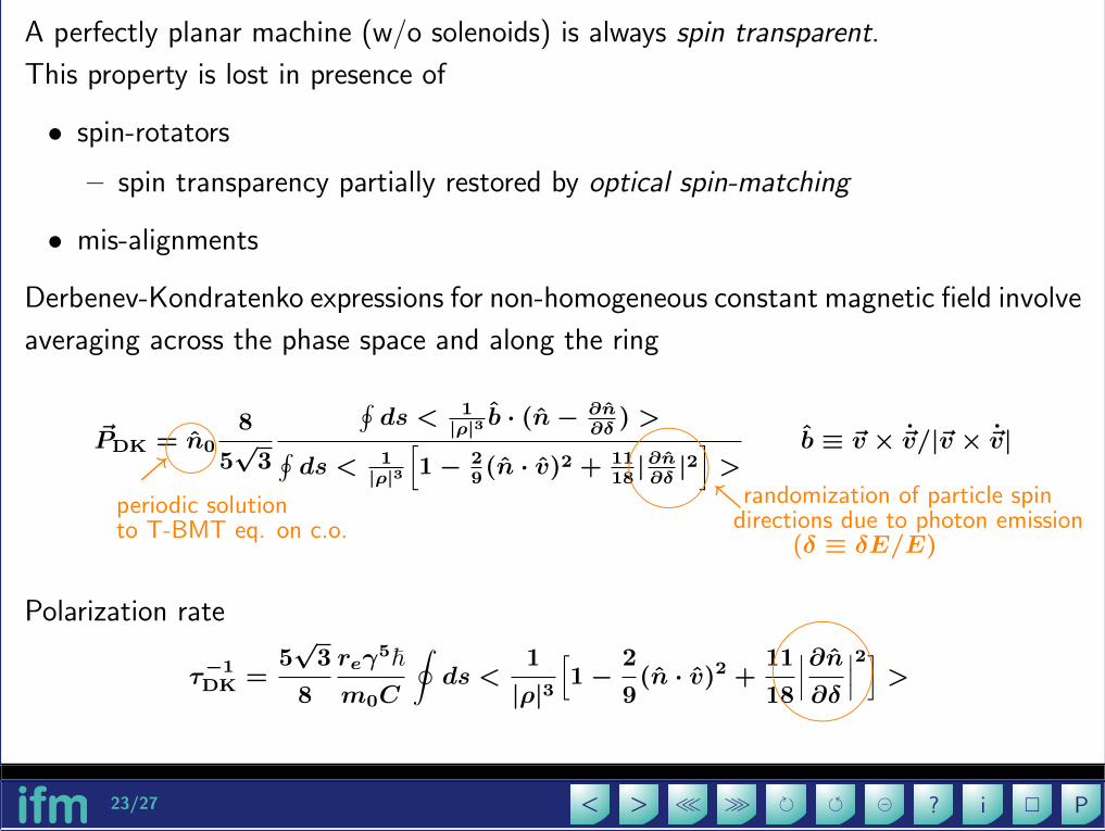
A perfectly planar machine (w/o solenoids) is always spin transparent.
This property is lost in presence of
• spin-rotators
– spin transparency partially restored by optical spin-matching
• mis-alignments
Derbenev-Kondratenko expressions for non-homogeneous constant magnetic field involve
averaging across the phase space and along the ring
~PDK = n0
8
5√3
∮ds < 1
|ρ|3 b · (n−∂n∂δ
) >∮ds < 1
|ρ|3
[1− 2
9(n · v)2 + 11
18|∂n∂δ|2]>
b ≡ ~v × ~v/|~v × ~v|����↗periodic solutionto T-BMT eq. on c.o.
����
↖randomization of particle spindirections due to photon emission
(δ ≡ δE/E)
Polarization rate
τ−1DK =
5√3
8
reγ5~
m0C
∮ds <
1
|ρ|3[1−
2
9(n · v)2 +
11
18
∣∣∣∂n∂δ
∣∣∣2] >&%'$

24/27 P�i?��≫≪><
Perfectly planar machine (w/o solenoids): ∂n/∂δ=0.
In general ∂n/∂δ 6=0 and large when
νspin ±mQx ± nQy ± pQs = integer νspin ' aγ
• Polarization time may be greatly reduced.
• PDK < PST.

25/27 P�i?��≫≪><
Tools
Accurate simulations are necessary for evaluating the polarization level
to be expected in presence of misalignments. Evaluation of D-K expressions is difficult.
• MAD-X used for simulating quadrupole misalignments and orbit correction
• SITROS (by J. Kewisch) used for computing the resulting polarization.
– Tracking code with 2nd order orbit description and non-linear spin motion.
– Used for HERA-e in the version improved by M. Boge and M. Berglund.
– It contains SITF (fully 6D) for analytical polarization computation with linearized
spin motion.
∗ Useful tool for preliminary checks before embarking in time consuming track-
ing.
∗ Computation of polarization related to the 3 degree of freedom separately:
useful for disentangling problems!

26/27 P�i?��≫≪><
Polarization evolution formulas
The exponential grow
P (t) = P∞(1− e−t/τp) + P (0)e−t/τp 1/τp = w∓ + w±
follows from the fact that
dn+
dt= n−w∓ − n+w± and
dn−
dt= n+w± − n−w∓
The Derbenev-Kondratenko polarization rate
τ−1DK =
5√3
8
reγ5~
m0C
∮<
1
|ρ|3[1−
2
9(n · v)2 +
11
18
∣∣∣∂n∂δ
∣∣∣2] >may be written as
τ−1DK = τ−1
p ' τ−1BKS + τ−1
d
with
τ−1BKS =
5√3
8
reγ5~
m0C
∮ds
1
|ρ|3[1−
2
9(n0 · v0)2
]and
τ−1d =
5√3
8
reγ5~
m0C
∮ds <
1
|ρ|3[1118
∣∣∣∂n∂δ
∣∣∣2] >
27/27 P�i?��≫≪><
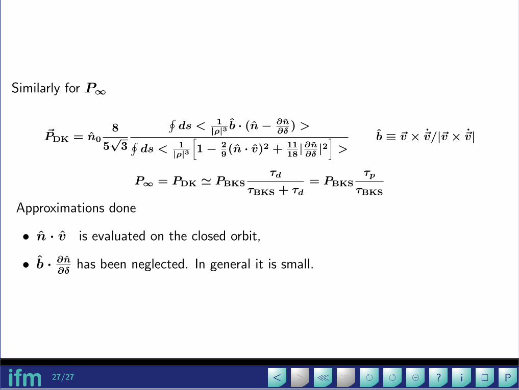
Similarly for P∞
~PDK = n0
8
5√3
∮ds < 1
|ρ|3 b · (n−∂n∂δ
) >∮ds < 1
|ρ|3
[1− 2
9(n · v)2 + 11
18|∂n∂δ|2]>
b ≡ ~v × ~v/|~v × ~v|
P∞ = PDK ' PBKS
τd
τBKS + τd= PBKS
τp
τBKS
Approximations done
• n · v is evaluated on the closed orbit,
• b · ∂n∂δ
has been neglected. In general it is small.