ERDAS Field Guide™

Volume One

October 2007

Copyright © 2007 Leica Geosystems Geospatial Imaging, LLC

All rights reserved.

Printed in the United States of America.

The information contained in this document is the exclusive property of Leica Geosystems Geospatial Imaging, LLC. This work is protected under United States copyright law and other international copyright treaties and conventions. No part of this work may be reproduced or transmitted in any form or by any means, electronic or mechanical, including photocopying and recording, or by any information storage or retrieval system, except as expressly permitted in writing by Leica Geosystems Geospatial Imaging, LLC. All requests should be sent to the attention of:

Manager, Technical DocumentationLeica Geosystems Geospatial Imaging, LLC.5051 Peachtree Corners CircleSuite 100Norcross, GA 30092-2500 USA.

The information contained in this document is subject to change without notice.

Government Reserved Rights. MrSID technology incorporated in the Software was developed in part through a project at the Los Alamos National Laboratory, funded by the U.S. Government, managed under contract by the University of California (University), and is under exclusive commercial license to LizardTech, Inc. It is used under license from LizardTech. MrSID is protected by U.S. Patent No. 5,710,835. Foreign patents pending. The U.S. Government and the University have reserved rights in MrSID technology, including without limitation: (a) The U.S. Government has a non-exclusive, nontransferable, irrevocable, paid-up license to practice or have practiced throughout the world, for or on behalf of the United States, inventions covered by U.S. Patent No. 5,710,835 and has other rights under 35 U.S.C. § 200-212 and applicable implementing regulations; (b) If LizardTech's rights in the MrSID Technology terminate during the term of this Agreement, you may continue to use the Software. Any provisions of this license which could reasonably be deemed to do so would then protect the University and/or the U.S. Government; and (c) The University has no obligation to furnish any know-how, technical assistance, or technical data to users of MrSID software and makes no warranty or representation as to the validity of U.S. Patent 5,710,835 nor that the MrSID Software will not infringe any patent or other proprietary right. For further information about these provisions, contact LizardTech, 1008 Western Ave., Suite 200, Seattle, WA 98104.

ERDAS, ERDAS IMAGINE, IMAGINE OrthoBASE, Stereo Analyst and IMAGINE VirtualGIS are registered trademarks; IMAGINE OrthoBASE Pro is a trademark of Leica Geosystems Geospatial Imaging, LLC.

SOCET SET is a registered trademark of BAE Systems Mission Solutions.

Other companies and products mentioned herein are trademarks or registered trademarks of their respective owners.

II-iii

Table of ContentsVolume One

Table of Contents . . . . . . . . . . . . . . . . . . . . . . . . . . . . . . . . . . . . . . . . . . . . . . . xi

List of Figures . . . . . . . . . . . . . . . . . . . . . . . . . . . . . . . . . . . . . . . . . . . . . . . . . xxv

List of Tables . . . . . . . . . . . . . . . . . . . . . . . . . . . . . . . . . . . . . . . . . . . . . . . . . . xxxi

Preface. . . . . . . . . . . . . . . . . . . . . . . . . . . . . . . . . . . . . . . . . . . . . . . . . . . . . . xxxv

Raster Data . . . . . . . . . . . . . . . . . . . . . . . . . . . . . . . . . . I-1Introduction . . . . . . . . . . . . . . . . . . . . . . . . . . . . . . I-1

Image Data . . . . . . . . . . . . . . . . . . . . . . . . . . . . . . . I-1Bands . . . . . . . . . . . . . . . . . . . . . . . . . . . . . . . . . . . . . . I-2Coordinate Systems . . . . . . . . . . . . . . . . . . . . . . . . . . . . I-3

Remote Sensing . . . . . . . . . . . . . . . . . . . . . . . . . . . I-4Absorption / Reflection Spectra . . . . . . . . . . . . . . . . . . . . I-6

Resolution . . . . . . . . . . . . . . . . . . . . . . . . . . . . . . I-14Spectral Resolution . . . . . . . . . . . . . . . . . . . . . . . . . . . . I-14Spatial Resolution . . . . . . . . . . . . . . . . . . . . . . . . . . . . . I-15Radiometric Resolution . . . . . . . . . . . . . . . . . . . . . . . . . I-16Temporal Resolution . . . . . . . . . . . . . . . . . . . . . . . . . . . I-17

Data Correction . . . . . . . . . . . . . . . . . . . . . . . . . . . I-17Line Dropout . . . . . . . . . . . . . . . . . . . . . . . . . . . . . . . . I-18Striping . . . . . . . . . . . . . . . . . . . . . . . . . . . . . . . . . . . . I-18

Data Storage . . . . . . . . . . . . . . . . . . . . . . . . . . . . I-18Storage Formats . . . . . . . . . . . . . . . . . . . . . . . . . . . . . . I-18Storage Media . . . . . . . . . . . . . . . . . . . . . . . . . . . . . . . I-21Calculating Disk Space . . . . . . . . . . . . . . . . . . . . . . . . . I-23ERDAS IMAGINE Format (.img) . . . . . . . . . . . . . . . . . . . I-24

Image File Organization . . . . . . . . . . . . . . . . . . . . I-27Consistent Naming Convention . . . . . . . . . . . . . . . . . . . . I-28Keeping Track of Image Files . . . . . . . . . . . . . . . . . . . . . I-28

Geocoded Data . . . . . . . . . . . . . . . . . . . . . . . . . . . I-29

Using Image Data in GIS . . . . . . . . . . . . . . . . . . . . I-29Subsetting and Mosaicking . . . . . . . . . . . . . . . . . . . . . . . I-29Enhancement . . . . . . . . . . . . . . . . . . . . . . . . . . . . . . . . I-30Multispectral Classification . . . . . . . . . . . . . . . . . . . . . . . I-31

Editing Raster Data . . . . . . . . . . . . . . . . . . . . . . . . I-31Editing Continuous (Athematic) Data . . . . . . . . . . . . . . . I-32Interpolation Techniques . . . . . . . . . . . . . . . . . . . . . . . . I-32

Vector Data . . . . . . . . . . . . . . . . . . . . . . . . . . . . . . . . . I-35Introduction . . . . . . . . . . . . . . . . . . . . . . . . . . . . . I-35

Points . . . . . . . . . . . . . . . . . . . . . . . . . . . . . . . . . . . . . I-35Lines . . . . . . . . . . . . . . . . . . . . . . . . . . . . . . . . . . . . . . I-36

II-iv

Polygons . . . . . . . . . . . . . . . . . . . . . . . . . . . . . . . . . . . I-36Vertex . . . . . . . . . . . . . . . . . . . . . . . . . . . . . . . . . . . . . I-36Coordinates . . . . . . . . . . . . . . . . . . . . . . . . . . . . . . . . . I-36Vector Layers . . . . . . . . . . . . . . . . . . . . . . . . . . . . . . . . I-37Topology . . . . . . . . . . . . . . . . . . . . . . . . . . . . . . . . . . . I-37Vector Files . . . . . . . . . . . . . . . . . . . . . . . . . . . . . . . . . I-37

Attribute Information . . . . . . . . . . . . . . . . . . . . . . I-39

Displaying Vector Data . . . . . . . . . . . . . . . . . . . . . I-40Color Schemes . . . . . . . . . . . . . . . . . . . . . . . . . . . . . . . I-40Symbolization . . . . . . . . . . . . . . . . . . . . . . . . . . . . . . . I-40

Vector Data Sources . . . . . . . . . . . . . . . . . . . . . . . I-42

Digitizing . . . . . . . . . . . . . . . . . . . . . . . . . . . . . . . I-42Tablet Digitizing . . . . . . . . . . . . . . . . . . . . . . . . . . . . . . I-42Screen Digitizing . . . . . . . . . . . . . . . . . . . . . . . . . . . . . I-44

Imported Vector Data . . . . . . . . . . . . . . . . . . . . . . I-44

Raster to Vector Conversion . . . . . . . . . . . . . . . . . I-45

Other Vector Data Types . . . . . . . . . . . . . . . . . . . . I-46Shapefile Vector Format . . . . . . . . . . . . . . . . . . . . . . . . I-46SDE . . . . . . . . . . . . . . . . . . . . . . . . . . . . . . . . . . . . . . I-46SDTS . . . . . . . . . . . . . . . . . . . . . . . . . . . . . . . . . . . . . I-47ArcGIS Integration . . . . . . . . . . . . . . . . . . . . . . . . . . . . I-47

Raster and Vector Data Sources . . . . . . . . . . . . . . . . . . . I-49Importing and Exporting . . . . . . . . . . . . . . . . . . . . I-49

Raster Data . . . . . . . . . . . . . . . . . . . . . . . . . . . . . . . . . I-49Raster Data Sources . . . . . . . . . . . . . . . . . . . . . . . . . . . I-53Annotation Data . . . . . . . . . . . . . . . . . . . . . . . . . . . . . . I-54Generic Binary Data . . . . . . . . . . . . . . . . . . . . . . . . . . . I-55Vector Data . . . . . . . . . . . . . . . . . . . . . . . . . . . . . . . . . I-55

Satellite Data . . . . . . . . . . . . . . . . . . . . . . . . . . . . I-56Satellite System . . . . . . . . . . . . . . . . . . . . . . . . . . . . . . I-57Satellite Characteristics . . . . . . . . . . . . . . . . . . . . . . . . . I-57IKONOS . . . . . . . . . . . . . . . . . . . . . . . . . . . . . . . . . . . . I-58IRS . . . . . . . . . . . . . . . . . . . . . . . . . . . . . . . . . . . . . . . I-59Landsat 1-5 . . . . . . . . . . . . . . . . . . . . . . . . . . . . . . . . . I-61Landsat 7 . . . . . . . . . . . . . . . . . . . . . . . . . . . . . . . . . . I-65NLAPS . . . . . . . . . . . . . . . . . . . . . . . . . . . . . . . . . . . . . I-66NOAA Polar Orbiter Data . . . . . . . . . . . . . . . . . . . . . . . . I-67OrbView-3 . . . . . . . . . . . . . . . . . . . . . . . . . . . . . . . . . . I-68SeaWiFS . . . . . . . . . . . . . . . . . . . . . . . . . . . . . . . . . . . I-69SPOT . . . . . . . . . . . . . . . . . . . . . . . . . . . . . . . . . . . . . . I-70SPOT4 . . . . . . . . . . . . . . . . . . . . . . . . . . . . . . . . . . . . . I-72

Radar Data . . . . . . . . . . . . . . . . . . . . . . . . . . . . . . I-72Advantages of Using Radar Data . . . . . . . . . . . . . . . . . . I-73Radar Sensors . . . . . . . . . . . . . . . . . . . . . . . . . . . . . . . I-73Speckle Noise . . . . . . . . . . . . . . . . . . . . . . . . . . . . . . . . I-76Applications for Radar Data . . . . . . . . . . . . . . . . . . . . . . I-76Current Radar Sensors . . . . . . . . . . . . . . . . . . . . . . . . . I-77Future Radar Sensors . . . . . . . . . . . . . . . . . . . . . . . . . . I-83

Image Data from Aircraft . . . . . . . . . . . . . . . . . . . I-83

II-v

AIRSAR . . . . . . . . . . . . . . . . . . . . . . . . . . . . . . . . . . . . I-83AVIRIS . . . . . . . . . . . . . . . . . . . . . . . . . . . . . . . . . . . . I-84Daedalus TMS . . . . . . . . . . . . . . . . . . . . . . . . . . . . . . . I-84

Image Data from Scanning . . . . . . . . . . . . . . . . . . I-84Photogrammetric Scanners . . . . . . . . . . . . . . . . . . . . . . I-85Desktop Scanners . . . . . . . . . . . . . . . . . . . . . . . . . . . . . I-85Aerial Photography . . . . . . . . . . . . . . . . . . . . . . . . . . . . I-86DOQs . . . . . . . . . . . . . . . . . . . . . . . . . . . . . . . . . . . . . I-86

ADRG Data . . . . . . . . . . . . . . . . . . . . . . . . . . . . . . I-86ARC System . . . . . . . . . . . . . . . . . . . . . . . . . . . . . . . . . I-87ADRG File Format . . . . . . . . . . . . . . . . . . . . . . . . . . . . . I-87.OVR (overview) . . . . . . . . . . . . . . . . . . . . . . . . . . . . . . I-88.IMG (scanned image data) . . . . . . . . . . . . . . . . . . . . . . I-89.Lxx (legend data) . . . . . . . . . . . . . . . . . . . . . . . . . . . . I-89ADRG File Naming Convention . . . . . . . . . . . . . . . . . . . . I-91

ADRI Data . . . . . . . . . . . . . . . . . . . . . . . . . . . . . . . I-92.OVR (overview) . . . . . . . . . . . . . . . . . . . . . . . . . . . . . . I-93.IMG (scanned image data) . . . . . . . . . . . . . . . . . . . . . . I-94ADRI File Naming Convention . . . . . . . . . . . . . . . . . . . . . I-94

Raster Product Format . . . . . . . . . . . . . . . . . . . . . I-95CIB . . . . . . . . . . . . . . . . . . . . . . . . . . . . . . . . . . . . . . . I-96CADRG . . . . . . . . . . . . . . . . . . . . . . . . . . . . . . . . . . . . I-96

Topographic Data . . . . . . . . . . . . . . . . . . . . . . . . . I-97DEM . . . . . . . . . . . . . . . . . . . . . . . . . . . . . . . . . . . . . . I-98DTED . . . . . . . . . . . . . . . . . . . . . . . . . . . . . . . . . . . . . I-99Using Topographic Data . . . . . . . . . . . . . . . . . . . . . . . . . I-99

GPS Data. . . . . . . . . . . . . . . . . . . . . . . . . . . . . . . I-100Introduction . . . . . . . . . . . . . . . . . . . . . . . . . . . . . . . . I-100Satellite Position . . . . . . . . . . . . . . . . . . . . . . . . . . . . . I-100Differential Correction . . . . . . . . . . . . . . . . . . . . . . . . . I-101Applications of GPS Data . . . . . . . . . . . . . . . . . . . . . . . I-101

Ordering Raster Data . . . . . . . . . . . . . . . . . . . . . I-103Addresses to Contact . . . . . . . . . . . . . . . . . . . . . . . . . I-103

Raster Data from Other Software Vendors . . . . . . I-106ERDAS Ver. 7.X . . . . . . . . . . . . . . . . . . . . . . . . . . . . . I-106GRID and GRID Stacks . . . . . . . . . . . . . . . . . . . . . . . . I-107JFIF (JPEG) . . . . . . . . . . . . . . . . . . . . . . . . . . . . . . . . I-107MrSID . . . . . . . . . . . . . . . . . . . . . . . . . . . . . . . . . . . . I-108SDTS . . . . . . . . . . . . . . . . . . . . . . . . . . . . . . . . . . . . I-108SUN Raster . . . . . . . . . . . . . . . . . . . . . . . . . . . . . . . . I-109TIFF . . . . . . . . . . . . . . . . . . . . . . . . . . . . . . . . . . . . . I-109GeoTIFF . . . . . . . . . . . . . . . . . . . . . . . . . . . . . . . . . . I-111

Vector Data from Other Software Vendors . . . . . . I-111ARCGEN . . . . . . . . . . . . . . . . . . . . . . . . . . . . . . . . . . I-112AutoCAD (DXF) . . . . . . . . . . . . . . . . . . . . . . . . . . . . . I-112DLG . . . . . . . . . . . . . . . . . . . . . . . . . . . . . . . . . . . . . I-113ETAK . . . . . . . . . . . . . . . . . . . . . . . . . . . . . . . . . . . . . I-114IGES . . . . . . . . . . . . . . . . . . . . . . . . . . . . . . . . . . . . . I-115TIGER . . . . . . . . . . . . . . . . . . . . . . . . . . . . . . . . . . . . I-115

II-vi

Image Display . . . . . . . . . . . . . . . . . . . . . . . . . . . . . . I-117Display Memory Size . . . . . . . . . . . . . . . . . . . . . . . . . . I-117Pixel . . . . . . . . . . . . . . . . . . . . . . . . . . . . . . . . . . . . . I-118Colors . . . . . . . . . . . . . . . . . . . . . . . . . . . . . . . . . . . . I-118Colormap and Colorcells . . . . . . . . . . . . . . . . . . . . . . . I-119Display Types . . . . . . . . . . . . . . . . . . . . . . . . . . . . . . . I-1218-bit PseudoColor . . . . . . . . . . . . . . . . . . . . . . . . . . . . I-12124-bit DirectColor . . . . . . . . . . . . . . . . . . . . . . . . . . . . I-12224-bit TrueColor . . . . . . . . . . . . . . . . . . . . . . . . . . . . . I-123PC Displays . . . . . . . . . . . . . . . . . . . . . . . . . . . . . . . . I-124

Displaying Raster Layers . . . . . . . . . . . . . . . . . . . I-125Continuous Raster Layers . . . . . . . . . . . . . . . . . . . . . . I-125Thematic Raster Layers . . . . . . . . . . . . . . . . . . . . . . . . I-130

Using the Viewer . . . . . . . . . . . . . . . . . . . . . . . . . I-133Pyramid Layers . . . . . . . . . . . . . . . . . . . . . . . . . . . . . . I-134Dithering . . . . . . . . . . . . . . . . . . . . . . . . . . . . . . . . . . I-137Viewing Layers . . . . . . . . . . . . . . . . . . . . . . . . . . . . . . I-138Viewing Multiple Layers . . . . . . . . . . . . . . . . . . . . . . . . I-139Linking Viewers . . . . . . . . . . . . . . . . . . . . . . . . . . . . . I-140Zoom and Roam . . . . . . . . . . . . . . . . . . . . . . . . . . . . . I-141Geographic Information . . . . . . . . . . . . . . . . . . . . . . . . I-142Enhancing Continuous Raster Layers . . . . . . . . . . . . . . . I-142Creating New Image Files . . . . . . . . . . . . . . . . . . . . . . I-143

Geographic Information Systems. . . . . . . . . . . . . . . . . . I-145Information vs. Data . . . . . . . . . . . . . . . . . . . . . . . . . . I-146

Data Input . . . . . . . . . . . . . . . . . . . . . . . . . . . . . I-147

Continuous Layers. . . . . . . . . . . . . . . . . . . . . . . . I-149

Thematic Layers . . . . . . . . . . . . . . . . . . . . . . . . . I-150Statistics . . . . . . . . . . . . . . . . . . . . . . . . . . . . . . . . . . I-151

Vector Layers . . . . . . . . . . . . . . . . . . . . . . . . . . . I-152

Attributes . . . . . . . . . . . . . . . . . . . . . . . . . . . . . . I-152Raster Attributes . . . . . . . . . . . . . . . . . . . . . . . . . . . . I-153Vector Attributes . . . . . . . . . . . . . . . . . . . . . . . . . . . . I-154

Analysis . . . . . . . . . . . . . . . . . . . . . . . . . . . . . . . I-155ERDAS IMAGINE Analysis Tools . . . . . . . . . . . . . . . . . . I-155Analysis Procedures . . . . . . . . . . . . . . . . . . . . . . . . . . I-156

Proximity Analysis . . . . . . . . . . . . . . . . . . . . . . . I-157

Contiguity Analysis . . . . . . . . . . . . . . . . . . . . . . . I-158

Neighborhood Analysis . . . . . . . . . . . . . . . . . . . . I-159

Recoding . . . . . . . . . . . . . . . . . . . . . . . . . . . . . . . I-161

Overlaying . . . . . . . . . . . . . . . . . . . . . . . . . . . . . I-162

Indexing . . . . . . . . . . . . . . . . . . . . . . . . . . . . . . . I-163

Matrix Analysis . . . . . . . . . . . . . . . . . . . . . . . . . . I-165

Modeling . . . . . . . . . . . . . . . . . . . . . . . . . . . . . . . I-165

Graphical Modeling . . . . . . . . . . . . . . . . . . . . . . . I-166

II-vii

Objects . . . . . . . . . . . . . . . . . . . . . . . . . . . . . . . . . . . I-170Data Types . . . . . . . . . . . . . . . . . . . . . . . . . . . . . . . . I-171Output Parameters . . . . . . . . . . . . . . . . . . . . . . . . . . . I-172Using Attributes in Models . . . . . . . . . . . . . . . . . . . . . . I-172

Script Modeling . . . . . . . . . . . . . . . . . . . . . . . . . . I-173Variables . . . . . . . . . . . . . . . . . . . . . . . . . . . . . . . . . . I-177

Vector Analysis . . . . . . . . . . . . . . . . . . . . . . . . . . I-177Editing Vector Layers . . . . . . . . . . . . . . . . . . . . . . . . . I-177

Constructing Topology . . . . . . . . . . . . . . . . . . . . I-178Building and Cleaning Coverages . . . . . . . . . . . . . . . . . I-179

Cartography . . . . . . . . . . . . . . . . . . . . . . . . . . . . . . . I-183Types of Maps . . . . . . . . . . . . . . . . . . . . . . . . . . . I-183

Thematic Maps . . . . . . . . . . . . . . . . . . . . . . . . . . . . . . I-185

Annotation . . . . . . . . . . . . . . . . . . . . . . . . . . . . . I-187

Scale. . . . . . . . . . . . . . . . . . . . . . . . . . . . . . . . . . I-188

Legends . . . . . . . . . . . . . . . . . . . . . . . . . . . . . . . I-192

Neatlines, Tick Marks, and Grid Lines . . . . . . . . . I-192

Symbols . . . . . . . . . . . . . . . . . . . . . . . . . . . . . . . I-193

Labels and Descriptive Text. . . . . . . . . . . . . . . . . I-194Typography and Lettering . . . . . . . . . . . . . . . . . . . . . . I-195

Projections . . . . . . . . . . . . . . . . . . . . . . . . . . . . . I-198Properties of Map Projections . . . . . . . . . . . . . . . . . . . . I-198Projection Types . . . . . . . . . . . . . . . . . . . . . . . . . . . . . I-200

Geographical and Planar Coordinates . . . . . . . . . I-202

Available Map Projections . . . . . . . . . . . . . . . . . . I-203

Choosing a Map Projection . . . . . . . . . . . . . . . . . I-210Map Projection Uses in a GIS . . . . . . . . . . . . . . . . . . . . I-210Deciding Factors . . . . . . . . . . . . . . . . . . . . . . . . . . . . . I-210Guidelines . . . . . . . . . . . . . . . . . . . . . . . . . . . . . . . . . I-210

Spheroids . . . . . . . . . . . . . . . . . . . . . . . . . . . . . . I-211

Map Composition . . . . . . . . . . . . . . . . . . . . . . . . . I-216Learning Map Composition . . . . . . . . . . . . . . . . . . . . . . I-216Plan the Map . . . . . . . . . . . . . . . . . . . . . . . . . . . . . . . I-216

Map Accuracy . . . . . . . . . . . . . . . . . . . . . . . . . . . I-217US National Map Accuracy Standard . . . . . . . . . . . . . . . I-217USGS Land Use and Land Cover Map Guidelines . . . . . . . I-218USDA SCS Soils Maps Guidelines . . . . . . . . . . . . . . . . . I-218Digitized Hardcopy Maps . . . . . . . . . . . . . . . . . . . . . . . I-218

Rectification . . . . . . . . . . . . . . . . . . . . . . . . . . . . . . . I-219Registration . . . . . . . . . . . . . . . . . . . . . . . . . . . . . . . . I-219Georeferencing . . . . . . . . . . . . . . . . . . . . . . . . . . . . . . I-220Latitude/Longitude . . . . . . . . . . . . . . . . . . . . . . . . . . . I-220Orthorectification . . . . . . . . . . . . . . . . . . . . . . . . . . . . I-220

When to Rectify . . . . . . . . . . . . . . . . . . . . . . . . . I-220When to Georeference Only . . . . . . . . . . . . . . . . . . . . . I-221

II-viii

Disadvantages of Rectification . . . . . . . . . . . . . . . . . . . I-222Rectification Steps . . . . . . . . . . . . . . . . . . . . . . . . . . . I-222

Ground Control Points . . . . . . . . . . . . . . . . . . . . . I-223GCPs in ERDAS IMAGINE . . . . . . . . . . . . . . . . . . . . . . . I-223Entering GCPs . . . . . . . . . . . . . . . . . . . . . . . . . . . . . . I-223GCP Prediction and Matching . . . . . . . . . . . . . . . . . . . . I-224

Polynomial Transformation . . . . . . . . . . . . . . . . . I-226Linear Transformations . . . . . . . . . . . . . . . . . . . . . . . . I-227Nonlinear Transformations . . . . . . . . . . . . . . . . . . . . . . I-229Effects of Order . . . . . . . . . . . . . . . . . . . . . . . . . . . . . I-231Minimum Number of GCPs . . . . . . . . . . . . . . . . . . . . . . I-235

Rubber Sheeting . . . . . . . . . . . . . . . . . . . . . . . . . I-236Triangle-Based Finite Element Analysis . . . . . . . . . . . . . I-236Triangulation . . . . . . . . . . . . . . . . . . . . . . . . . . . . . . . I-236Triangle-based rectification . . . . . . . . . . . . . . . . . . . . . I-237Linear transformation . . . . . . . . . . . . . . . . . . . . . . . . . I-237Nonlinear transformation . . . . . . . . . . . . . . . . . . . . . . . I-237Check Point Analysis . . . . . . . . . . . . . . . . . . . . . . . . . . I-238

RMS Error . . . . . . . . . . . . . . . . . . . . . . . . . . . . . . I-238Residuals and RMS Error Per GCP . . . . . . . . . . . . . . . . . I-238Total RMS Error . . . . . . . . . . . . . . . . . . . . . . . . . . . . . I-239Error Contribution by Point . . . . . . . . . . . . . . . . . . . . . I-240Tolerance of RMS Error . . . . . . . . . . . . . . . . . . . . . . . . I-240Evaluating RMS Error . . . . . . . . . . . . . . . . . . . . . . . . . I-240

Resampling Methods . . . . . . . . . . . . . . . . . . . . . . I-241Rectifying to Lat/Lon . . . . . . . . . . . . . . . . . . . . . . . . . . I-243Nearest Neighbor . . . . . . . . . . . . . . . . . . . . . . . . . . . . I-243Bilinear Interpolation . . . . . . . . . . . . . . . . . . . . . . . . . . I-244Cubic Convolution . . . . . . . . . . . . . . . . . . . . . . . . . . . . I-247Bicubic Spline Interpolation . . . . . . . . . . . . . . . . . . . . . I-250

Map-to-Map Coordinate Conversions . . . . . . . . . . I-252Conversion Process . . . . . . . . . . . . . . . . . . . . . . . . . . . I-252Vector Data . . . . . . . . . . . . . . . . . . . . . . . . . . . . . . . . I-253

Hardcopy Output . . . . . . . . . . . . . . . . . . . . . . . . . . . . I-255Printing Maps . . . . . . . . . . . . . . . . . . . . . . . . . . . I-255

Scaled Maps . . . . . . . . . . . . . . . . . . . . . . . . . . . . . . . . I-255Printing Large Maps . . . . . . . . . . . . . . . . . . . . . . . . . . I-255Scale and Resolution . . . . . . . . . . . . . . . . . . . . . . . . . . I-256Map Scaling Examples . . . . . . . . . . . . . . . . . . . . . . . . . I-257

Mechanics of Printing . . . . . . . . . . . . . . . . . . . . . I-259Halftone Printing . . . . . . . . . . . . . . . . . . . . . . . . . . . . . I-259Continuous Tone Printing . . . . . . . . . . . . . . . . . . . . . . . I-260Contrast and Color Tables . . . . . . . . . . . . . . . . . . . . . . I-260RGB to CMY Conversion . . . . . . . . . . . . . . . . . . . . . . . . I-261

Map Projections . . . . . . . . . . . . . . . . . . . . . . . . . . . . . I-263USGS Projections . . . . . . . . . . . . . . . . . . . . . . I-264

Alaska Conformal . . . . . . . . . . . . . . . . . . . . . . I-267

II-ix

Albers Conical Equal Area . . . . . . . . . . . . . . . I-269

Azimuthal Equidistant . . . . . . . . . . . . . . . . . . I-272

Behrmann . . . . . . . . . . . . . . . . . . . . . . . . . . . I-275

Bonne . . . . . . . . . . . . . . . . . . . . . . . . . . . . . . I-277

Cassini . . . . . . . . . . . . . . . . . . . . . . . . . . . . . I-279

Eckert I . . . . . . . . . . . . . . . . . . . . . . . . . . . . . I-281

Eckert II . . . . . . . . . . . . . . . . . . . . . . . . . . . . I-283

Eckert III . . . . . . . . . . . . . . . . . . . . . . . . . . . I-285

Eckert IV . . . . . . . . . . . . . . . . . . . . . . . . . . . . I-287

Eckert V . . . . . . . . . . . . . . . . . . . . . . . . . . . . I-289

Eckert VI . . . . . . . . . . . . . . . . . . . . . . . . . . . . I-291

EOSAT SOM . . . . . . . . . . . . . . . . . . . . . . . . . . I-293

Equidistant Conic . . . . . . . . . . . . . . . . . . . . . . I-294

Equidistant Cylindrical . . . . . . . . . . . . . . . . . . I-296

Equirectangular (Plate Carrée) . . . . . . . . . . . I-297

Gall Stereographic . . . . . . . . . . . . . . . . . . . . . I-299

Gauss Kruger . . . . . . . . . . . . . . . . . . . . . . . . . I-300

General Vertical Near-side Perspective . . . . . I-301

Geographic (Lat/Lon) . . . . . . . . . . . . . . . . . . I-303

Gnomonic . . . . . . . . . . . . . . . . . . . . . . . . . . . I-305

Hammer . . . . . . . . . . . . . . . . . . . . . . . . . . . . I-307

Interrupted Goode Homolosine . . . . . . . . . . . I-309

Interrupted Mollweide . . . . . . . . . . . . . . . . . . I-311

Lambert Azimuthal Equal Area . . . . . . . . . . . . I-312

Lambert Conformal Conic . . . . . . . . . . . . . . . . I-315

Loximuthal . . . . . . . . . . . . . . . . . . . . . . . . . . I-318

Mercator . . . . . . . . . . . . . . . . . . . . . . . . . . . . I-320

Miller Cylindrical . . . . . . . . . . . . . . . . . . . . . . I-323

Modified Transverse Mercator . . . . . . . . . . . . I-325

Mollweide . . . . . . . . . . . . . . . . . . . . . . . . . . . I-327

New Zealand Map Grid . . . . . . . . . . . . . . . . . . I-329

Oblated Equal Area . . . . . . . . . . . . . . . . . . . . I-330

Oblique Mercator (Hotine) . . . . . . . . . . . . . . . I-331

Orthographic . . . . . . . . . . . . . . . . . . . . . . . . . I-334

Plate Carrée . . . . . . . . . . . . . . . . . . . . . . . . . I-337

Polar Stereographic . . . . . . . . . . . . . . . . . . . . I-338

Polyconic . . . . . . . . . . . . . . . . . . . . . . . . . . . . I-341

Quartic Authalic . . . . . . . . . . . . . . . . . . . . . . . I-343

Robinson . . . . . . . . . . . . . . . . . . . . . . . . . . . . I-345

RSO . . . . . . . . . . . . . . . . . . . . . . . . . . . . . . . . I-347

II-x

Sinusoidal . . . . . . . . . . . . . . . . . . . . . . . . . . . I-348

Space Oblique Mercator . . . . . . . . . . . . . . . . . I-350

Space Oblique Mercator (Formats A & B) . . . . I-352

State Plane . . . . . . . . . . . . . . . . . . . . . . . . . . I-353

Stereographic . . . . . . . . . . . . . . . . . . . . . . . . I-363

Stereographic (Extended) . . . . . . . . . . . . . . . I-366

Transverse Mercator . . . . . . . . . . . . . . . . . . . I-367

Two Point Equidistant . . . . . . . . . . . . . . . . . . I-369

UTM . . . . . . . . . . . . . . . . . . . . . . . . . . . . . . . . I-371

Van der Grinten I . . . . . . . . . . . . . . . . . . . . . . I-374

Wagner IV . . . . . . . . . . . . . . . . . . . . . . . . . . . I-376

Wagner VII . . . . . . . . . . . . . . . . . . . . . . . . . . I-378

Winkel I . . . . . . . . . . . . . . . . . . . . . . . . . . . . I-380

External Projections . . . . . . . . . . . . . . . . . . . I-382

Bipolar Oblique Conic Conformal . . . . . . . . . . I-384

Cassini-Soldner . . . . . . . . . . . . . . . . . . . . . . . I-385

Laborde Oblique Mercator . . . . . . . . . . . . . . . I-387

Minimum Error Conformal . . . . . . . . . . . . . . . I-388

Modified Polyconic . . . . . . . . . . . . . . . . . . . . . I-389

Modified Stereographic . . . . . . . . . . . . . . . . . I-390

Mollweide Equal Area . . . . . . . . . . . . . . . . . . . I-391

Rectified Skew Orthomorphic . . . . . . . . . . . . . I-393

Robinson Pseudocylindrical . . . . . . . . . . . . . . I-394

Southern Orientated Gauss Conformal . . . . . . I-395

Swiss Cylindrical . . . . . . . . . . . . . . . . . . . . . . I-396

Winkel’s Tripel . . . . . . . . . . . . . . . . . . . . . . . I-397Volume Two

Mosaic . . . . . . . . . . . . . . . . . . . . . . . . . . . . . . . . . . . . II-1Input Image Mode. . . . . . . . . . . . . . . . . . . . . . . . . II-2

Exclude Areas . . . . . . . . . . . . . . . . . . . . . . . . . . . . . . . II-2Image Dodging . . . . . . . . . . . . . . . . . . . . . . . . . . . . . . . II-2Color Balancing . . . . . . . . . . . . . . . . . . . . . . . . . . . . . . II-3Histogram Matching . . . . . . . . . . . . . . . . . . . . . . . . . . . II-4

Intersection Mode . . . . . . . . . . . . . . . . . . . . . . . . . II-5Set Overlap Function . . . . . . . . . . . . . . . . . . . . . . . . . . . II-6Automatically Generate Cutlines For Intersection . . . . . . . II-6Geometry-based Cutline Generation . . . . . . . . . . . . . . . . II-7

Output Image Mode. . . . . . . . . . . . . . . . . . . . . . . . II-8Output Image Options . . . . . . . . . . . . . . . . . . . . . . . . . . II-8Run Mosaic To Disc . . . . . . . . . . . . . . . . . . . . . . . . . . . II-10

II-xi

Enhancement . . . . . . . . . . . . . . . . . . . . . . . . . . . . . . . II-11Display vs. File Enhancement . . . . . . . . . . . . . . . . . . . . II-12Spatial Modeling Enhancements . . . . . . . . . . . . . . . . . . II-12

Correcting Data . . . . . . . . . . . . . . . . . . . . . . . . . . II-15Radiometric Correction: Visible/Infrared Imagery . . . . . . II-16Atmospheric Effects . . . . . . . . . . . . . . . . . . . . . . . . . . II-17Geometric Correction . . . . . . . . . . . . . . . . . . . . . . . . . II-18

Radiometric Enhancement . . . . . . . . . . . . . . . . . . II-18Contrast Stretching . . . . . . . . . . . . . . . . . . . . . . . . . . . II-19Histogram Equalization . . . . . . . . . . . . . . . . . . . . . . . . II-24Histogram Matching . . . . . . . . . . . . . . . . . . . . . . . . . . II-27Brightness Inversion . . . . . . . . . . . . . . . . . . . . . . . . . . II-28

Spatial Enhancement . . . . . . . . . . . . . . . . . . . . . . II-28Convolution Filtering . . . . . . . . . . . . . . . . . . . . . . . . . . II-29Crisp . . . . . . . . . . . . . . . . . . . . . . . . . . . . . . . . . . . . . II-34Resolution Merge . . . . . . . . . . . . . . . . . . . . . . . . . . . . II-34Adaptive Filter . . . . . . . . . . . . . . . . . . . . . . . . . . . . . . II-36

Wavelet Resolution Merge . . . . . . . . . . . . . . . . . . II-38Wavelet Theory . . . . . . . . . . . . . . . . . . . . . . . . . . . . . II-38Algorithm Theory . . . . . . . . . . . . . . . . . . . . . . . . . . . . II-41Prerequisites and Limitations . . . . . . . . . . . . . . . . . . . . II-43Spectral Transform . . . . . . . . . . . . . . . . . . . . . . . . . . . II-44

Spectral Enhancement . . . . . . . . . . . . . . . . . . . . . II-45Principal Components Analysis . . . . . . . . . . . . . . . . . . . II-46Decorrelation Stretch . . . . . . . . . . . . . . . . . . . . . . . . . II-50Tasseled Cap . . . . . . . . . . . . . . . . . . . . . . . . . . . . . . . II-50RGB to IHS . . . . . . . . . . . . . . . . . . . . . . . . . . . . . . . . II-52IHS to RGB . . . . . . . . . . . . . . . . . . . . . . . . . . . . . . . . II-54Indices . . . . . . . . . . . . . . . . . . . . . . . . . . . . . . . . . . . II-55

Hyperspectral Image Processing . . . . . . . . . . . . . II-58Normalize . . . . . . . . . . . . . . . . . . . . . . . . . . . . . . . . . II-59IAR Reflectance . . . . . . . . . . . . . . . . . . . . . . . . . . . . . II-60Log Residuals . . . . . . . . . . . . . . . . . . . . . . . . . . . . . . . II-60Rescale . . . . . . . . . . . . . . . . . . . . . . . . . . . . . . . . . . . II-60Processing Sequence . . . . . . . . . . . . . . . . . . . . . . . . . . II-61Spectrum Average . . . . . . . . . . . . . . . . . . . . . . . . . . . II-62Signal to Noise . . . . . . . . . . . . . . . . . . . . . . . . . . . . . . II-62Mean per Pixel . . . . . . . . . . . . . . . . . . . . . . . . . . . . . . II-62Profile Tools . . . . . . . . . . . . . . . . . . . . . . . . . . . . . . . . II-62Wavelength Axis . . . . . . . . . . . . . . . . . . . . . . . . . . . . . II-64Spectral Library . . . . . . . . . . . . . . . . . . . . . . . . . . . . . II-64Classification . . . . . . . . . . . . . . . . . . . . . . . . . . . . . . . II-65System Requirements . . . . . . . . . . . . . . . . . . . . . . . . . II-65

Fourier Analysis . . . . . . . . . . . . . . . . . . . . . . . . . II-65FFT . . . . . . . . . . . . . . . . . . . . . . . . . . . . . . . . . . . . . . II-67Fourier Magnitude . . . . . . . . . . . . . . . . . . . . . . . . . . . . II-68IFFT . . . . . . . . . . . . . . . . . . . . . . . . . . . . . . . . . . . . . II-71Filtering . . . . . . . . . . . . . . . . . . . . . . . . . . . . . . . . . . . II-72Windows . . . . . . . . . . . . . . . . . . . . . . . . . . . . . . . . . . II-74Fourier Noise Removal . . . . . . . . . . . . . . . . . . . . . . . . II-77Homomorphic Filtering . . . . . . . . . . . . . . . . . . . . . . . . II-78

II-xii

Radar Imagery Enhancement. . . . . . . . . . . . . . . . II-79Speckle Noise . . . . . . . . . . . . . . . . . . . . . . . . . . . . . . . II-80Edge Detection . . . . . . . . . . . . . . . . . . . . . . . . . . . . . . II-87Texture . . . . . . . . . . . . . . . . . . . . . . . . . . . . . . . . . . . II-90Radiometric Correction: Radar Imagery . . . . . . . . . . . . . II-93Slant-to-Ground Range Correction . . . . . . . . . . . . . . . . II-95Merging Radar with VIS/IR Imagery . . . . . . . . . . . . . . . II-96

Classification . . . . . . . . . . . . . . . . . . . . . . . . . . . . . . . II-99The Classification Process . . . . . . . . . . . . . . . . . . II-99

Pattern Recognition . . . . . . . . . . . . . . . . . . . . . . . . . . . II-99Training . . . . . . . . . . . . . . . . . . . . . . . . . . . . . . . . . . . II-99Signatures . . . . . . . . . . . . . . . . . . . . . . . . . . . . . . . . II-100Decision Rule . . . . . . . . . . . . . . . . . . . . . . . . . . . . . . II-101Output File . . . . . . . . . . . . . . . . . . . . . . . . . . . . . . . . II-101

Classification Tips . . . . . . . . . . . . . . . . . . . . . . . .II-102Classification Scheme . . . . . . . . . . . . . . . . . . . . . . . . II-102Iterative Classification . . . . . . . . . . . . . . . . . . . . . . . . II-102Supervised vs. Unsupervised Training . . . . . . . . . . . . . II-103Classifying Enhanced Data . . . . . . . . . . . . . . . . . . . . . II-103Dimensionality . . . . . . . . . . . . . . . . . . . . . . . . . . . . . II-103

Supervised Training . . . . . . . . . . . . . . . . . . . . . .II-104Training Samples and Feature Space Objects . . . . . . . . II-105

Selecting Training Samples . . . . . . . . . . . . . . . . .II-105Evaluating Training Samples . . . . . . . . . . . . . . . . . . . II-107

Selecting Feature Space Objects . . . . . . . . . . . . .II-108

Unsupervised Training . . . . . . . . . . . . . . . . . . . .II-111ISODATA Clustering . . . . . . . . . . . . . . . . . . . . . . . . . II-112RGB Clustering . . . . . . . . . . . . . . . . . . . . . . . . . . . . . II-115

Signature Files . . . . . . . . . . . . . . . . . . . . . . . . . .II-118

Evaluating Signatures . . . . . . . . . . . . . . . . . . . . .II-119Alarm . . . . . . . . . . . . . . . . . . . . . . . . . . . . . . . . . . . II-120Ellipse . . . . . . . . . . . . . . . . . . . . . . . . . . . . . . . . . . . II-121Contingency Matrix . . . . . . . . . . . . . . . . . . . . . . . . . . II-122Separability . . . . . . . . . . . . . . . . . . . . . . . . . . . . . . . II-123Signature Manipulation . . . . . . . . . . . . . . . . . . . . . . . II-126

Classification Decision Rules . . . . . . . . . . . . . . . .II-127Nonparametric Rules . . . . . . . . . . . . . . . . . . . . . . . . . II-127Parametric Rules . . . . . . . . . . . . . . . . . . . . . . . . . . . II-128Parallelepiped . . . . . . . . . . . . . . . . . . . . . . . . . . . . . . II-129Feature Space . . . . . . . . . . . . . . . . . . . . . . . . . . . . . II-132Minimum Distance . . . . . . . . . . . . . . . . . . . . . . . . . . II-133Mahalanobis Distance . . . . . . . . . . . . . . . . . . . . . . . . II-135Maximum Likelihood/Bayesian . . . . . . . . . . . . . . . . . . II-136

Fuzzy Methodology . . . . . . . . . . . . . . . . . . . . . . .II-138Fuzzy Classification . . . . . . . . . . . . . . . . . . . . . . . . . . II-138Fuzzy Convolution . . . . . . . . . . . . . . . . . . . . . . . . . . . II-138

Expert Classification . . . . . . . . . . . . . . . . . . . . . .II-139Knowledge Engineer . . . . . . . . . . . . . . . . . . . . . . . . . II-140Knowledge Classifier . . . . . . . . . . . . . . . . . . . . . . . . . II-142

II-xiii

Evaluating Classification . . . . . . . . . . . . . . . . . . .II-142Thresholding . . . . . . . . . . . . . . . . . . . . . . . . . . . . . . II-143Accuracy Assessment . . . . . . . . . . . . . . . . . . . . . . . . II-145

Photogrammetric Concepts . . . . . . . . . . . . . . . . . . . . . .II-149What is Photogrammetry? . . . . . . . . . . . . . . . . . . . . . II-149Types of Photographs and Images . . . . . . . . . . . . . . . II-150Why use Photogrammetry? . . . . . . . . . . . . . . . . . . . . II-151Photogrammetry/ Conventional Geometric Correction . . II-151Single Frame Orthorectification/Block Triangulation . . . II-152

Image and Data Acquisition . . . . . . . . . . . . . . . .II-154Photogrammetric Scanners . . . . . . . . . . . . . . . . . . . . II-155Desktop Scanners . . . . . . . . . . . . . . . . . . . . . . . . . . . II-155Scanning Resolutions . . . . . . . . . . . . . . . . . . . . . . . . II-156Coordinate Systems . . . . . . . . . . . . . . . . . . . . . . . . . II-157Terrestrial Photography . . . . . . . . . . . . . . . . . . . . . . . II-160

Interior Orientation . . . . . . . . . . . . . . . . . . . . . .II-161Principal Point and Focal Length . . . . . . . . . . . . . . . . . II-162Fiducial Marks . . . . . . . . . . . . . . . . . . . . . . . . . . . . . II-162Lens Distortion . . . . . . . . . . . . . . . . . . . . . . . . . . . . . II-164

Exterior Orientation . . . . . . . . . . . . . . . . . . . . . .II-165The Collinearity Equation . . . . . . . . . . . . . . . . . . . . . . II-167

Photogrammetric Solutions . . . . . . . . . . . . . . . . .II-168Space Resection . . . . . . . . . . . . . . . . . . . . . . . . . . . . II-169Space Forward Intersection . . . . . . . . . . . . . . . . . . . . II-169Bundle Block Adjustment . . . . . . . . . . . . . . . . . . . . . . II-170Least Squares Adjustment . . . . . . . . . . . . . . . . . . . . . II-173Self-calibrating Bundle Adjustment . . . . . . . . . . . . . . . II-176Automatic Gross Error Detection . . . . . . . . . . . . . . . . . II-176

GCPs . . . . . . . . . . . . . . . . . . . . . . . . . . . . . . . . . .II-177GCP Requirements . . . . . . . . . . . . . . . . . . . . . . . . . . II-178Processing Multiple Strips of Imagery . . . . . . . . . . . . . II-179

Tie Points . . . . . . . . . . . . . . . . . . . . . . . . . . . . . .II-180Automatic Tie Point Collection . . . . . . . . . . . . . . . . . . II-180

Image Matching Techniques . . . . . . . . . . . . . . . .II-181Area Based Matching . . . . . . . . . . . . . . . . . . . . . . . . . II-182Feature Based Matching . . . . . . . . . . . . . . . . . . . . . . II-184Relation Based Matching . . . . . . . . . . . . . . . . . . . . . . II-184Image Pyramid . . . . . . . . . . . . . . . . . . . . . . . . . . . . II-185

Satellite Photogrammetry . . . . . . . . . . . . . . . . . .II-185SPOT Interior Orientation . . . . . . . . . . . . . . . . . . . . . II-187SPOT Exterior Orientation . . . . . . . . . . . . . . . . . . . . . II-188Collinearity Equations & Satellite Block Triangulation . . II-192

Terrain Analysis . . . . . . . . . . . . . . . . . . . . . . . . . . . . .II-197Terrain Data . . . . . . . . . . . . . . . . . . . . . . . . . . . .II-198

Slope Images . . . . . . . . . . . . . . . . . . . . . . . . . . .II-199

Aspect Images . . . . . . . . . . . . . . . . . . . . . . . . . .II-201

Shaded Relief . . . . . . . . . . . . . . . . . . . . . . . . . . .II-203

II-xiv

Topographic Normalization . . . . . . . . . . . . . . . . .II-204Lambertian Reflectance Model . . . . . . . . . . . . . . . . . . II-205Non-Lambertian Model . . . . . . . . . . . . . . . . . . . . . . . II-206

Radar Concepts . . . . . . . . . . . . . . . . . . . . . . . . . . . . .II-207IMAGINE OrthoRadar Theory . . . . . . . . . . . . . . . .II-207

Parameters Required for Orthorectification . . . . . . . . . II-207Algorithm Description . . . . . . . . . . . . . . . . . . . . . . . . II-210

IMAGINE StereoSAR DEM Theory . . . . . . . . . . . . .II-215Introduction . . . . . . . . . . . . . . . . . . . . . . . . . . . . . . . II-215Input . . . . . . . . . . . . . . . . . . . . . . . . . . . . . . . . . . . . II-216Subset . . . . . . . . . . . . . . . . . . . . . . . . . . . . . . . . . . II-218Despeckle . . . . . . . . . . . . . . . . . . . . . . . . . . . . . . . . II-218Degrade . . . . . . . . . . . . . . . . . . . . . . . . . . . . . . . . . II-219Register . . . . . . . . . . . . . . . . . . . . . . . . . . . . . . . . . . II-219Constrain . . . . . . . . . . . . . . . . . . . . . . . . . . . . . . . . . II-220Match . . . . . . . . . . . . . . . . . . . . . . . . . . . . . . . . . . . II-220Degrade . . . . . . . . . . . . . . . . . . . . . . . . . . . . . . . . . II-225Height . . . . . . . . . . . . . . . . . . . . . . . . . . . . . . . . . . . II-225

IMAGINE InSAR Theory . . . . . . . . . . . . . . . . . . . .II-226Introduction . . . . . . . . . . . . . . . . . . . . . . . . . . . . . . . II-226Electromagnetic Wave Background . . . . . . . . . . . . . . . II-226The Interferometric Model . . . . . . . . . . . . . . . . . . . . . II-229Image Registration . . . . . . . . . . . . . . . . . . . . . . . . . . II-234Phase Noise Reduction . . . . . . . . . . . . . . . . . . . . . . . II-236Phase Flattening . . . . . . . . . . . . . . . . . . . . . . . . . . . . II-237Phase Unwrapping . . . . . . . . . . . . . . . . . . . . . . . . . . II-238Conclusions . . . . . . . . . . . . . . . . . . . . . . . . . . . . . . . II-241

Math Topics . . . . . . . . . . . . . . . . . . . . . . . . . . . . . . . .II-243Summation . . . . . . . . . . . . . . . . . . . . . . . . . . . . .II-243

Statistics . . . . . . . . . . . . . . . . . . . . . . . . . . . . . .II-243Histogram . . . . . . . . . . . . . . . . . . . . . . . . . . . . . . . . II-243Bin Functions . . . . . . . . . . . . . . . . . . . . . . . . . . . . . . II-244Mean . . . . . . . . . . . . . . . . . . . . . . . . . . . . . . . . . . . . II-246Normal Distribution . . . . . . . . . . . . . . . . . . . . . . . . . . II-247Variance . . . . . . . . . . . . . . . . . . . . . . . . . . . . . . . . . II-248Standard Deviation . . . . . . . . . . . . . . . . . . . . . . . . . . II-249Parameters . . . . . . . . . . . . . . . . . . . . . . . . . . . . . . . II-249Covariance . . . . . . . . . . . . . . . . . . . . . . . . . . . . . . . . II-250Covariance Matrix . . . . . . . . . . . . . . . . . . . . . . . . . . . II-251

Dimensionality of Data . . . . . . . . . . . . . . . . . . . .II-251Measurement Vector . . . . . . . . . . . . . . . . . . . . . . . . . II-251Mean Vector . . . . . . . . . . . . . . . . . . . . . . . . . . . . . . . II-252Feature Space . . . . . . . . . . . . . . . . . . . . . . . . . . . . . II-253Feature Space Images . . . . . . . . . . . . . . . . . . . . . . . . II-253n-Dimensional Histogram . . . . . . . . . . . . . . . . . . . . . II-254Spectral Distance . . . . . . . . . . . . . . . . . . . . . . . . . . . II-255

Polynomials . . . . . . . . . . . . . . . . . . . . . . . . . . . .II-255Order . . . . . . . . . . . . . . . . . . . . . . . . . . . . . . . . . . . II-255Transformation Matrix . . . . . . . . . . . . . . . . . . . . . . . . II-256

II-xv

Matrix Algebra . . . . . . . . . . . . . . . . . . . . . . . . . .II-257Matrix Notation . . . . . . . . . . . . . . . . . . . . . . . . . . . . II-257Matrix Multiplication . . . . . . . . . . . . . . . . . . . . . . . . . II-257Transposition . . . . . . . . . . . . . . . . . . . . . . . . . . . . . . II-258

Glossary . . . . . . . . . . . . . . . . . . . . . . . . . . . . . . . . . .II-261

Bibliography . . . . . . . . . . . . . . . . . . . . . . . . . . . . . . .II-317Works Cited . . . . . . . . . . . . . . . . . . . . . . . . . . . .II-317

Related Reading . . . . . . . . . . . . . . . . . . . . . . . . .II-329

Index . . . . . . . . . . . . . . . . . . . . . . . . . . . . . . . . . . . .II-333

II-xvi

II-xvii

List of FiguresFigure I-1: Pixels and Bands in a Raster Image. . . . . . . . . . . . . . . . . . . . . . . . . . . I-2Figure I-2: Typical File Coordinates . . . . . . . . . . . . . . . . . . . . . . . . . . . . . . . . . . I-4Figure I-3: Electromagnetic Spectrum . . . . . . . . . . . . . . . . . . . . . . . . . . . . . . . . I-5Figure I-4: Sun Illumination Spectral Irradiance at the Earth’s Surface . . . . . . . . . . I-7Figure I-5: Factors Affecting Radiation . . . . . . . . . . . . . . . . . . . . . . . . . . . . . . . . I-8Figure I-6: Reflectance Spectra . . . . . . . . . . . . . . . . . . . . . . . . . . . . . . . . . . . . .I-10Figure I-7: Laboratory Spectra of Clay Minerals in the Infrared Region . . . . . . . . . .I-12Figure I-8: IFOV . . . . . . . . . . . . . . . . . . . . . . . . . . . . . . . . . . . . . . . . . . . . . . .I-16Figure I-9: Brightness Values . . . . . . . . . . . . . . . . . . . . . . . . . . . . . . . . . . . . . .I-17Figure I-10: Landsat TM—Band 2 (Four Types of Resolution) . . . . . . . . . . . . . . . . . .I-17Figure I-11: Band Interleaved by Line (BIL) . . . . . . . . . . . . . . . . . . . . . . . . . . . . .I-19Figure I-12: Band Sequential (BSQ) . . . . . . . . . . . . . . . . . . . . . . . . . . . . . . . . . .I-20Figure I-13: Image Files Store Raster Layers . . . . . . . . . . . . . . . . . . . . . . . . . . . .I-24Figure I-14: Example of a Thematic Raster Layer . . . . . . . . . . . . . . . . . . . . . . . . .I-25Figure I-15: Examples of Continuous Raster Layers . . . . . . . . . . . . . . . . . . . . . . . .I-26Figure I-16: Vector Elements . . . . . . . . . . . . . . . . . . . . . . . . . . . . . . . . . . . . . . .I-35Figure I-17: Vertices . . . . . . . . . . . . . . . . . . . . . . . . . . . . . . . . . . . . . . . . . . . .I-36Figure I-18: Workspace Structure . . . . . . . . . . . . . . . . . . . . . . . . . . . . . . . . . . . .I-38Figure I-19: Attribute CellArray . . . . . . . . . . . . . . . . . . . . . . . . . . . . . . . . . . . . .I-39Figure I-20: Symbolization Example . . . . . . . . . . . . . . . . . . . . . . . . . . . . . . . . . .I-41Figure I-21: Digitizing Tablet . . . . . . . . . . . . . . . . . . . . . . . . . . . . . . . . . . . . . . .I-42Figure I-22: Raster Format Converted to Vector Format . . . . . . . . . . . . . . . . . . . .I-45Figure I-23: Multispectral Imagery Comparison. . . . . . . . . . . . . . . . . . . . . . . . . . .I-58Figure I-24: Landsat MSS vs. Landsat TM . . . . . . . . . . . . . . . . . . . . . . . . . . . . . .I-64Figure I-25: SPOT Panchromatic vs. SPOT XS . . . . . . . . . . . . . . . . . . . . . . . . . . . .I-71Figure I-26: SLAR Radar . . . . . . . . . . . . . . . . . . . . . . . . . . . . . . . . . . . . . . . . .I-74Figure I-27: Received Radar Signal . . . . . . . . . . . . . . . . . . . . . . . . . . . . . . . . . . .I-74Figure I-28: Radar Reflection from Different Sources and Distances . . . . . . . . . . . .I-75Figure I-29: ADRG Overview File Displayed in a Viewer . . . . . . . . . . . . . . . . . . . . .I-88Figure I-30: Subset Area with Overlapping ZDRs . . . . . . . . . . . . . . . . . . . . . . . . .I-89Figure I-31: Seamless Nine Image DR . . . . . . . . . . . . . . . . . . . . . . . . . . . . . . . . .I-93Figure I-32: ADRI Overview File Displayed in a Viewer . . . . . . . . . . . . . . . . . . . . . .I-94Figure I-33: Arc/second Format . . . . . . . . . . . . . . . . . . . . . . . . . . . . . . . . . . . . .I-98Figure I-34: Common Uses of GPS Data . . . . . . . . . . . . . . . . . . . . . . . . . . . . . . I-102Figure I-35: Example of One Seat with One Display and Two Screens . . . . . . . . . . . I-117Figure I-36: Transforming Data File Values to a Colorcell Value . . . . . . . . . . . . . . I-121Figure I-37: Transforming Data File Values to a Colorcell Value . . . . . . . . . . . . . . I-123Figure I-38: Transforming Data File Values to Screen Values . . . . . . . . . . . . . . . . I-124Figure I-39: Contrast Stretch and Colorcell Values . . . . . . . . . . . . . . . . . . . . . . . I-127Figure I-40: Stretching by Min/Max vs. Standard Deviation . . . . . . . . . . . . . . . . . I-128Figure I-41: Continuous Raster Layer Display Process . . . . . . . . . . . . . . . . . . . . I-129Figure I-42: Thematic Raster Layer Display Process . . . . . . . . . . . . . . . . . . . . . . I-132Figure I-43: Pyramid Layers . . . . . . . . . . . . . . . . . . . . . . . . . . . . . . . . . . . . . . I-136Figure I-44: Example of Dithering . . . . . . . . . . . . . . . . . . . . . . . . . . . . . . . . . . I-137Figure I-45: Example of Color Patches . . . . . . . . . . . . . . . . . . . . . . . . . . . . . . . I-138Figure I-46: Linked Viewers . . . . . . . . . . . . . . . . . . . . . . . . . . . . . . . . . . . . . . I-141Figure I-47: Data Input . . . . . . . . . . . . . . . . . . . . . . . . . . . . . . . . . . . . . . . . . I-148Figure I-48: Raster Attributes for lnlandc.img . . . . . . . . . . . . . . . . . . . . . . . . . . I-153Figure I-49: Vector Attributes CellArray. . . . . . . . . . . . . . . . . . . . . . . . . . . . . . . I-155Figure I-50: Proximity Analysis . . . . . . . . . . . . . . . . . . . . . . . . . . . . . . . . . . . . I-158

II-xviii

Figure I-51: Contiguity Analysis . . . . . . . . . . . . . . . . . . . . . . . . . . . . . . . . . . . . I-158Figure I-52: Using a Mask . . . . . . . . . . . . . . . . . . . . . . . . . . . . . . . . . . . . . . . I-160Figure I-53: Sum Option of Neighborhood Analysis (Image Interpreter) . . . . . . . . . I-161Figure I-54: Overlay . . . . . . . . . . . . . . . . . . . . . . . . . . . . . . . . . . . . . . . . . . I-163Figure I-55: Indexing . . . . . . . . . . . . . . . . . . . . . . . . . . . . . . . . . . . . . . . . . . I-164Figure I-56: Graphical Model for Sensitivity Analysis . . . . . . . . . . . . . . . . . . . . . . I-167Figure I-57: Graphical Model Structure . . . . . . . . . . . . . . . . . . . . . . . . . . . . . . . I-168Figure I-58: Modeling Objects . . . . . . . . . . . . . . . . . . . . . . . . . . . . . . . . . . . . . I-171Figure I-59: Graphical and Script Models For Tasseled Cap Transformation . . . . . . I-175Figure I-60: Layer Errors . . . . . . . . . . . . . . . . . . . . . . . . . . . . . . . . . . . . . . . . I-181Figure I-61: Sample Scale Bars . . . . . . . . . . . . . . . . . . . . . . . . . . . . . . . . . . . . I-188Figure I-62: Sample Legend . . . . . . . . . . . . . . . . . . . . . . . . . . . . . . . . . . . . . . I-192Figure I-63: Sample Neatline, Tick Marks, and Grid Lines . . . . . . . . . . . . . . . . . . . I-193Figure I-64: Sample Symbols. . . . . . . . . . . . . . . . . . . . . . . . . . . . . . . . . . . . . . I-194Figure I-65: Sample Sans Serif and Serif Typefaces with Various Styles Applied . . . . I-196Figure I-66: Good Lettering vs. Bad Lettering . . . . . . . . . . . . . . . . . . . . . . . . . . . I-197Figure I-67: Projection Types . . . . . . . . . . . . . . . . . . . . . . . . . . . . . . . . . . . . . I-200Figure I-68: Tangent and Secant Cones . . . . . . . . . . . . . . . . . . . . . . . . . . . . . . . I-201Figure I-69: Tangent and Secant Cylinders . . . . . . . . . . . . . . . . . . . . . . . . . . . . I-202Figure I-70: Ellipse . . . . . . . . . . . . . . . . . . . . . . . . . . . . . . . . . . . . . . . . . . . . I-211Figure I-71: Polynomial Curve vs. GCPs . . . . . . . . . . . . . . . . . . . . . . . . . . . . . . . I-226Figure I-72: Linear Transformations . . . . . . . . . . . . . . . . . . . . . . . . . . . . . . . . . I-228Figure I-73: Nonlinear Transformations . . . . . . . . . . . . . . . . . . . . . . . . . . . . . . . I-229Figure I-74: Transformation Example—1st-Order . . . . . . . . . . . . . . . . . . . . . . . . I-232Figure I-75: Transformation Example—2nd GCP Changed . . . . . . . . . . . . . . . . . . . I-232Figure I-76: Transformation Example—2nd-Order . . . . . . . . . . . . . . . . . . . . . . . . I-233Figure I-77: Transformation Example—4th GCP Added . . . . . . . . . . . . . . . . . . . . . I-233Figure I-78: Transformation Example—3rd-Order . . . . . . . . . . . . . . . . . . . . . . . . I-234Figure I-79: Transformation Example—Effect of a 3rd-Order Transformation . . . . . . I-234Figure I-80: Triangle Network . . . . . . . . . . . . . . . . . . . . . . . . . . . . . . . . . . . . . I-236Figure I-81: Residuals and RMS Error Per Point. . . . . . . . . . . . . . . . . . . . . . . . . . I-239Figure I-82: RMS Error Tolerance . . . . . . . . . . . . . . . . . . . . . . . . . . . . . . . . . . . I-240Figure I-83: Resampling . . . . . . . . . . . . . . . . . . . . . . . . . . . . . . . . . . . . . . . . . I-242Figure I-84: Nearest Neighbor . . . . . . . . . . . . . . . . . . . . . . . . . . . . . . . . . . . . . I-243Figure I-85: Bilinear Interpolation . . . . . . . . . . . . . . . . . . . . . . . . . . . . . . . . . . I-245Figure I-86: Linear Interpolation . . . . . . . . . . . . . . . . . . . . . . . . . . . . . . . . . . . I-245Figure I-87: Cubic Convolution. . . . . . . . . . . . . . . . . . . . . . . . . . . . . . . . . . . . . I-248Figure I-88: Layout for a Book Map and a Paneled Map . . . . . . . . . . . . . . . . . . . . I-256Figure I-89: Sample Map Composition . . . . . . . . . . . . . . . . . . . . . . . . . . . . . . . . I-257Figure I-90: Albers Conical Equal Area Projection . . . . . . . . . . . . . . . . . . . . . . . . I-271Figure I-91: Polar Aspect of the Azimuthal Equidistant Projection . . . . . . . . . . . . . I-274Figure I-92: Behrmann Cylindrical Equal-Area Projection . . . . . . . . . . . . . . . . . . . I-276Figure I-93: Bonne Projection . . . . . . . . . . . . . . . . . . . . . . . . . . . . . . . . . . . . . I-278Figure I-94: Cassini Projection . . . . . . . . . . . . . . . . . . . . . . . . . . . . . . . . . . . . . I-280Figure I-95: Eckert I Projection . . . . . . . . . . . . . . . . . . . . . . . . . . . . . . . . . . . . I-282Figure I-96: Eckert II Projection. . . . . . . . . . . . . . . . . . . . . . . . . . . . . . . . . . . . I-284Figure I-97: Eckert III Projection . . . . . . . . . . . . . . . . . . . . . . . . . . . . . . . . . . . I-286Figure I-98: Eckert IV Projection . . . . . . . . . . . . . . . . . . . . . . . . . . . . . . . . . . . I-288Figure I-99: Eckert V Summary . . . . . . . . . . . . . . . . . . . . . . . . . . . . . . . . . . . . I-289Figure I-100: Eckert V Projection . . . . . . . . . . . . . . . . . . . . . . . . . . . . . . . . . . . I-290Figure I-101: Eckert VI Projection . . . . . . . . . . . . . . . . . . . . . . . . . . . . . . . . . . I-292Figure I-102: Equidistant Conic Projection . . . . . . . . . . . . . . . . . . . . . . . . . . . . . I-295Figure I-103: Equirectangular Projection . . . . . . . . . . . . . . . . . . . . . . . . . . . . . I-298Figure I-104: Geographic Projection . . . . . . . . . . . . . . . . . . . . . . . . . . . . . . . . . I-304

II-xix

Figure I-105: Hammer Projection . . . . . . . . . . . . . . . . . . . . . . . . . . . . . . . . . . . I-308Figure I-106: Interrupted Goode Homolosine Projection . . . . . . . . . . . . . . . . . . . . I-309Figure I-107: Interrupted Mollweide Projection . . . . . . . . . . . . . . . . . . . . . . . . . . I-311Figure I-108: Lambert Azimuthal Equal Area Projection . . . . . . . . . . . . . . . . . . . . I-314Figure I-109: Lambert Conformal Conic Projection . . . . . . . . . . . . . . . . . . . . . . . I-317Figure I-110: Loximuthal Projection . . . . . . . . . . . . . . . . . . . . . . . . . . . . . . . . . I-319Figure I-111: Mercator Projection . . . . . . . . . . . . . . . . . . . . . . . . . . . . . . . . . . . I-322Figure I-112: Miller Cylindrical Projection . . . . . . . . . . . . . . . . . . . . . . . . . . . . . I-324Figure I-113: Mollweide Projection . . . . . . . . . . . . . . . . . . . . . . . . . . . . . . . . . . I-328Figure I-114: Oblique Mercator Projection . . . . . . . . . . . . . . . . . . . . . . . . . . . . . I-333Figure I-115: Orthographic Projection . . . . . . . . . . . . . . . . . . . . . . . . . . . . . . . . I-336Figure I-116: Plate Carrée Projection . . . . . . . . . . . . . . . . . . . . . . . . . . . . . . . . I-337Figure I-117: Polar Stereographic Projection and its Geometric Construction . . . . . . I-340Figure I-118: Polyconic Projection of North America . . . . . . . . . . . . . . . . . . . . . . I-342Figure I-119: Quartic Authalic Projection . . . . . . . . . . . . . . . . . . . . . . . . . . . . . . I-344Figure I-120: Robinson Projection . . . . . . . . . . . . . . . . . . . . . . . . . . . . . . . . . . I-346Figure I-121: Sinusoidal Projection . . . . . . . . . . . . . . . . . . . . . . . . . . . . . . . . . . I-349Figure I-122: Space Oblique Mercator Projection . . . . . . . . . . . . . . . . . . . . . . . . . I-351Figure I-123: Zones of the State Plane Coordinate System . . . . . . . . . . . . . . . . . . I-354Figure I-124: Stereographic Projection . . . . . . . . . . . . . . . . . . . . . . . . . . . . . . . I-365Figure I-125: Two Point Equidistant Projection . . . . . . . . . . . . . . . . . . . . . . . . . . I-370Figure I-126: Zones of the Universal Transverse Mercator Grid in the United States . I-372Figure I-127: Van der Grinten I Projection . . . . . . . . . . . . . . . . . . . . . . . . . . . . . I-375Figure I-128: Wagner IV Projection . . . . . . . . . . . . . . . . . . . . . . . . . . . . . . . . . I-377Figure I-129: Wagner VII Projection . . . . . . . . . . . . . . . . . . . . . . . . . . . . . . . . . I-379Figure I-130: Winkel I Projection . . . . . . . . . . . . . . . . . . . . . . . . . . . . . . . . . . . I-381Figure I-131: Winkel’s Tripel Projection . . . . . . . . . . . . . . . . . . . . . . . . . . . . . . . I-397Figure II-1: Histograms of Radiometrically Enhanced Data . . . . . . . . . . . . . . . . . . II-19Figure II-2: Graph of a Lookup Table . . . . . . . . . . . . . . . . . . . . . . . . . . . . . . . . II-20Figure II-3: Enhancement with Lookup Tables . . . . . . . . . . . . . . . . . . . . . . . . . . II-20Figure II-4: Nonlinear Radiometric Enhancement . . . . . . . . . . . . . . . . . . . . . . . . II-21Figure II-5: Piecewise Linear Contrast Stretch . . . . . . . . . . . . . . . . . . . . . . . . . . II-22Figure II-6: Contrast Stretch Using Lookup Tables, and Effect on Histogram . . . . . . II-24Figure II-7: Histogram Equalization . . . . . . . . . . . . . . . . . . . . . . . . . . . . . . . . . II-24Figure II-8: Histogram Equalization Example . . . . . . . . . . . . . . . . . . . . . . . . . . . II-25Figure II-9: Equalized Histogram . . . . . . . . . . . . . . . . . . . . . . . . . . . . . . . . . . . II-26Figure II-10: Histogram Matching . . . . . . . . . . . . . . . . . . . . . . . . . . . . . . . . . . II-28Figure II-11: Spatial Frequencies . . . . . . . . . . . . . . . . . . . . . . . . . . . . . . . . . . II-29Figure II-12: Applying a Convolution Kernel . . . . . . . . . . . . . . . . . . . . . . . . . . . . II-30Figure II-13: Output Values for Convolution Kernel . . . . . . . . . . . . . . . . . . . . . . II-31Figure II-14: Local Luminance Intercept . . . . . . . . . . . . . . . . . . . . . . . . . . . . . . II-37Figure II-15: Schematic Diagram of the Discrete Wavelet Transform - DWT . . . . . . . II-40Figure II-16: Inverse Discrete Wavelet Transform - DWT-1 . . . . . . . . . . . . . . . . . . II-41Figure II-17: Wavelet Resolution Merge . . . . . . . . . . . . . . . . . . . . . . . . . . . . . . . II-42Figure II-18: Two Band Scatterplot . . . . . . . . . . . . . . . . . . . . . . . . . . . . . . . . . . II-46Figure II-19: First Principal Component . . . . . . . . . . . . . . . . . . . . . . . . . . . . . . . II-47Figure II-20: Range of First Principal Component . . . . . . . . . . . . . . . . . . . . . . . . II-47Figure II-21: Second Principal Component . . . . . . . . . . . . . . . . . . . . . . . . . . . . . II-48Figure II-22: Intensity, Hue, and Saturation Color Coordinate System . . . . . . . . . . II-53Figure II-23: Hyperspectral Data Axes . . . . . . . . . . . . . . . . . . . . . . . . . . . . . . . II-58Figure II-24: Rescale Graphical User Interface (GUI) . . . . . . . . . . . . . . . . . . . . . II-61Figure II-25: Spectrum Average GUI . . . . . . . . . . . . . . . . . . . . . . . . . . . . . . . . II-62Figure II-26: Spectral Profile . . . . . . . . . . . . . . . . . . . . . . . . . . . . . . . . . . . . . . II-63Figure II-27: Two-Dimensional Spatial Profile . . . . . . . . . . . . . . . . . . . . . . . . . . . II-63

II-xx

Figure II-28: Three-Dimensional Spatial Profile . . . . . . . . . . . . . . . . . . . . . . . . . II-64Figure II-29: Surface Profile . . . . . . . . . . . . . . . . . . . . . . . . . . . . . . . . . . . . . . II-64Figure II-30: One-Dimensional Fourier Analysis . . . . . . . . . . . . . . . . . . . . . . . . . II-67Figure II-31: Example of Fourier Magnitude . . . . . . . . . . . . . . . . . . . . . . . . . . . II-69Figure II-32: The Padding Technique . . . . . . . . . . . . . . . . . . . . . . . . . . . . . . . . II-71Figure II-33: Comparison of Direct and Fourier Domain Processing . . . . . . . . . . . . II-73Figure II-34: An Ideal Cross Section . . . . . . . . . . . . . . . . . . . . . . . . . . . . . . . . . II-75Figure II-35: High-Pass Filtering Using the Ideal Window . . . . . . . . . . . . . . . . . . . II-75Figure II-36: Filtering Using the Bartlett Window . . . . . . . . . . . . . . . . . . . . . . . . II-76Figure II-37: Filtering Using the Butterworth Window . . . . . . . . . . . . . . . . . . . . . II-76Figure II-38: Homomorphic Filtering Process . . . . . . . . . . . . . . . . . . . . . . . . . . . II-79Figure II-39: Effects of Mean and Median Filters . . . . . . . . . . . . . . . . . . . . . . . . II-82Figure II-40: Regions of Local Region Filter . . . . . . . . . . . . . . . . . . . . . . . . . . . . II-83Figure II-41: One-dimensional, Continuous Edge, and Line Models . . . . . . . . . . . . II-87Figure II-42: A Noisy Edge Superimposed on an Ideal Edge . . . . . . . . . . . . . . . . . II-88Figure II-43: Edge and Line Derivatives . . . . . . . . . . . . . . . . . . . . . . . . . . . . . . II-88Figure II-44: Adjust Brightness Function . . . . . . . . . . . . . . . . . . . . . . . . . . . . . II-94Figure II-45: Range Lines vs. Lines of Constant Range . . . . . . . . . . . . . . . . . . . . . II-95Figure II-46: Slant-to-Ground Range Correction . . . . . . . . . . . . . . . . . . . . . . . . . II-95Figure II-47: Example of a Feature Space Image . . . . . . . . . . . . . . . . . . . . . . . II-108Figure II-48: Process for Defining a Feature Space Object . . . . . . . . . . . . . . . . . II-110Figure II-49: ISODATA Arbitrary Clusters . . . . . . . . . . . . . . . . . . . . . . . . . . . . II-113Figure II-50: ISODATA First Pass . . . . . . . . . . . . . . . . . . . . . . . . . . . . . . . . . . II-113Figure II-51: ISODATA Second Pass . . . . . . . . . . . . . . . . . . . . . . . . . . . . . . . . II-114Figure II-52: RGB Clustering . . . . . . . . . . . . . . . . . . . . . . . . . . . . . . . . . . . . . II-117Figure II-53: Ellipse Evaluation of Signatures . . . . . . . . . . . . . . . . . . . . . . . . . II-122Figure II-54: Classification Flow Diagram . . . . . . . . . . . . . . . . . . . . . . . . . . . . II-129Figure II-55: Parallelepiped Classification With Two Standard Deviations as Limits . II-130Figure II-56: Parallelepiped Corners Compared to the Signature Ellipse . . . . . . . . II-132Figure II-57: Feature Space Classification . . . . . . . . . . . . . . . . . . . . . . . . . . . . II-132Figure II-58: Minimum Spectral Distance . . . . . . . . . . . . . . . . . . . . . . . . . . . . . II-134Figure II-59: Knowledge Engineer Editing Window . . . . . . . . . . . . . . . . . . . . . . II-140Figure II-60: Example of a Decision Tree Branch. . . . . . . . . . . . . . . . . . . . . . . . II-141Figure II-61: Split Rule Decision Tree Branch . . . . . . . . . . . . . . . . . . . . . . . . . . II-141Figure II-62: Knowledge Classifier Classes of Interest . . . . . . . . . . . . . . . . . . . . II-142Figure II-63: Histogram of a Distance Image . . . . . . . . . . . . . . . . . . . . . . . . . . II-143Figure II-64: Interactive Thresholding Tips . . . . . . . . . . . . . . . . . . . . . . . . . . . II-144Figure II-65: Exposure Stations Along a Flight Path . . . . . . . . . . . . . . . . . . . . . II-154Figure II-66: A Regular Rectangular Block of Aerial Photos . . . . . . . . . . . . . . . . II-155Figure II-67: Pixel Coordinates and Image Coordinates . . . . . . . . . . . . . . . . . . . II-158Figure II-68: Image Space and Ground Space Coordinate System . . . . . . . . . . . . II-159Figure II-69: Terrestrial Photography . . . . . . . . . . . . . . . . . . . . . . . . . . . . . . . II-160Figure II-70: Internal Geometry . . . . . . . . . . . . . . . . . . . . . . . . . . . . . . . . . . . II-161Figure II-71: Pixel Coordinate System vs. Image Space Coordinate System . . . . . . II-163Figure II-72: Radial vs. Tangential Lens Distortion . . . . . . . . . . . . . . . . . . . . . . II-164Figure II-73: Elements of Exterior Orientation . . . . . . . . . . . . . . . . . . . . . . . . . II-166Figure II-74: Space Forward Intersection. . . . . . . . . . . . . . . . . . . . . . . . . . . . . II-170Figure II-75: Photogrammetric Configuration . . . . . . . . . . . . . . . . . . . . . . . . . . II-171Figure II-76: GCP Configuration . . . . . . . . . . . . . . . . . . . . . . . . . . . . . . . . . . . II-179Figure II-77: GCPs in a Block of Images . . . . . . . . . . . . . . . . . . . . . . . . . . . . . II-179Figure II-78: Point Distribution for Triangulation . . . . . . . . . . . . . . . . . . . . . . . . II-180Figure II-79: Tie Points in a Block . . . . . . . . . . . . . . . . . . . . . . . . . . . . . . . . . II-180Figure II-80: Image Pyramid for Matching at Coarse to Full Resolution . . . . . . . . . II-185Figure II-81: Perspective Centers of SPOT Scan Lines . . . . . . . . . . . . . . . . . . . . II-186

II-xxi

Figure II-82: Image Coordinates in a Satellite Scene . . . . . . . . . . . . . . . . . . . . . II-187Figure II-83: Interior Orientation of a SPOT Scene . . . . . . . . . . . . . . . . . . . . . . II-188Figure II-84: Inclination of a Satellite Stereo-Scene (View from North to South) . . II-190Figure II-85: Velocity Vector and Orientation Angle of a Single Scene . . . . . . . . . II-191Figure II-86: Ideal Point Distribution Over a Satellite Scene for Triangulation . . . . II-192Figure II-87: Orthorectification . . . . . . . . . . . . . . . . . . . . . . . . . . . . . . . . . . . II-193Figure II-88: Digital Orthophoto—Finding Gray Values . . . . . . . . . . . . . . . . . . . . II-194Figure II-89: Regularly Spaced Terrain Data Points . . . . . . . . . . . . . . . . . . . . . II-198Figure II-90: 3 × 3 Window Calculates the Slope at Each Pixel . . . . . . . . . . . . . . II-199Figure II-91: Slope Calculation Example . . . . . . . . . . . . . . . . . . . . . . . . . . . . . II-201Figure II-92: 3 × 3 Window Calculates the Aspect at Each Pixel . . . . . . . . . . . . . II-202Figure II-93: Aspect Calculation Example. . . . . . . . . . . . . . . . . . . . . . . . . . . . . II-203Figure II-94: Shaded Relief . . . . . . . . . . . . . . . . . . . . . . . . . . . . . . . . . . . . . II-204Figure II-95: Doppler Cone . . . . . . . . . . . . . . . . . . . . . . . . . . . . . . . . . . . . . . II-213Figure II-96: Sparse Mapping and Output Grids . . . . . . . . . . . . . . . . . . . . . . . . II-214Figure II-97: IMAGINE StereoSAR DEM Process Flow . . . . . . . . . . . . . . . . . . . . . II-215Figure II-98: SAR Image Intersection . . . . . . . . . . . . . . . . . . . . . . . . . . . . . . . II-216Figure II-99: UL Corner of the Reference Image . . . . . . . . . . . . . . . . . . . . . . . . II-221Figure II-100: UL Corner of the Match Image . . . . . . . . . . . . . . . . . . . . . . . . . . II-221Figure II-101: Image Pyramid . . . . . . . . . . . . . . . . . . . . . . . . . . . . . . . . . . . . II-222Figure II-102: Electromagnetic Wave . . . . . . . . . . . . . . . . . . . . . . . . . . . . . . . II-227Figure II-103: Variation of Electric Field in Time . . . . . . . . . . . . . . . . . . . . . . . . II-227Figure II-104: Effect of Time and Distance on Energy . . . . . . . . . . . . . . . . . . . . II-228Figure II-105: Geometric Model for an Interferometric SAR System . . . . . . . . . . . II-229Figure II-106: Differential Collection Geometry . . . . . . . . . . . . . . . . . . . . . . . . II-233Figure II-107: Interferometric Phase Image without Filtering . . . . . . . . . . . . . . . II-236Figure II-108: Interferometric Phase Image with Filtering . . . . . . . . . . . . . . . . . II-237Figure II-109: Interferometric Phase Image without Phase Flattening . . . . . . . . . . II-238Figure II-110: Electromagnetic Wave Traveling through Space . . . . . . . . . . . . . . II-238Figure II-111: One-dimensional Continuous vs. Wrapped Phase Function . . . . . . . II-239Figure II-112: Sequence of Unwrapped Phase Images . . . . . . . . . . . . . . . . . . . . II-240Figure II-113: Wrapped vs. Unwrapped Phase Images . . . . . . . . . . . . . . . . . . . . II-241Figure II-114: Histogram . . . . . . . . . . . . . . . . . . . . . . . . . . . . . . . . . . . . . . . II-244Figure II-115: Normal Distribution . . . . . . . . . . . . . . . . . . . . . . . . . . . . . . . . . II-247Figure II-116: Measurement Vector . . . . . . . . . . . . . . . . . . . . . . . . . . . . . . . . II-252Figure II-117: Mean Vector . . . . . . . . . . . . . . . . . . . . . . . . . . . . . . . . . . . . . . II-252Figure II-118: Two Band Plot . . . . . . . . . . . . . . . . . . . . . . . . . . . . . . . . . . . . . II-253Figure II-119: Two-band Scatterplot . . . . . . . . . . . . . . . . . . . . . . . . . . . . . . . . II-254

II-xxii

II-xxiii

List of TablesTable I-1: Bandwidths Used in Remote Sensing . . . . . . . . . . . . . . . . . . . . . . . . . .I-13Table I-2: Description of File Types . . . . . . . . . . . . . . . . . . . . . . . . . . . . . . . . . .I-38Table I-3: Raster Data Formats . . . . . . . . . . . . . . . . . . . . . . . . . . . . . . . . . . . . .I-50Table I-4: Annotation Data Formats . . . . . . . . . . . . . . . . . . . . . . . . . . . . . . . . . .I-54Table I-5: Vector Data Formats . . . . . . . . . . . . . . . . . . . . . . . . . . . . . . . . . . . . .I-55Table I-6: IKONOS Bands and Wavelengths . . . . . . . . . . . . . . . . . . . . . . . . . . . . .I-59Table I-7: LISS-III Bands and Wavelengths . . . . . . . . . . . . . . . . . . . . . . . . . . . . .I-59Table I-8: Panchromatic Band and Wavelength . . . . . . . . . . . . . . . . . . . . . . . . . . .I-60Table I-9: WiFS Bands and Wavelengths . . . . . . . . . . . . . . . . . . . . . . . . . . . . . . .I-60Table I-10: MSS Bands and Wavelengths . . . . . . . . . . . . . . . . . . . . . . . . . . . . . . .I-61Table I-11: TM Bands and Wavelengths . . . . . . . . . . . . . . . . . . . . . . . . . . . . . . . .I-63Table I-12: Landsat 7 Characteristics . . . . . . . . . . . . . . . . . . . . . . . . . . . . . . . . .I-65Table I-13: AVHRR Bands and Wavelengths . . . . . . . . . . . . . . . . . . . . . . . . . . . . .I-68Table I-14: OrbView-3 Bands and Spectral Ranges . . . . . . . . . . . . . . . . . . . . . . . .I-69Table I-15: SeaWiFS Bands and Wavelengths . . . . . . . . . . . . . . . . . . . . . . . . . . . .I-69Table I-16: SPOT XS Bands and Wavelengths . . . . . . . . . . . . . . . . . . . . . . . . . . . .I-71Table I-17: SPOT4 Bands and Wavelengths . . . . . . . . . . . . . . . . . . . . . . . . . . . . .I-72Table I-18: Commonly Used Bands for Radar Imaging . . . . . . . . . . . . . . . . . . . . . .I-75Table I-19: Current Radar Sensors . . . . . . . . . . . . . . . . . . . . . . . . . . . . . . . . . . .I-77Table I-20: JERS-1 Bands and Wavelengths . . . . . . . . . . . . . . . . . . . . . . . . . . . . .I-80Table I-21: RADARSAT Beam Mode Resolution . . . . . . . . . . . . . . . . . . . . . . . . . . .I-80Table I-22: SIR-C/X-SAR Bands and Frequencies . . . . . . . . . . . . . . . . . . . . . . . . .I-82Table I-23: Daedalus TMS Bands and Wavelengths . . . . . . . . . . . . . . . . . . . . . . . .I-84Table I-24: ARC System Chart Types . . . . . . . . . . . . . . . . . . . . . . . . . . . . . . . . .I-90Table I-25: Legend Files for the ARC System Chart Types . . . . . . . . . . . . . . . . . . . .I-91Table I-26: Common Raster Data Products . . . . . . . . . . . . . . . . . . . . . . . . . . . . . I-103Table I-27: File Types Created by Screendump . . . . . . . . . . . . . . . . . . . . . . . . . . I-109Table I-28: The Most Common TIFF Format Elements . . . . . . . . . . . . . . . . . . . . . I-110Table I-29: Conversion of DXF Entries . . . . . . . . . . . . . . . . . . . . . . . . . . . . . . . . I-113Table I-30: Conversion of IGES Entities . . . . . . . . . . . . . . . . . . . . . . . . . . . . . . . I-115Table I-31: Colorcell Example . . . . . . . . . . . . . . . . . . . . . . . . . . . . . . . . . . . . . I-120Table I-32: Commonly Used RGB Colors . . . . . . . . . . . . . . . . . . . . . . . . . . . . . . I-131Table I-33: Overview of Zoom Ratio . . . . . . . . . . . . . . . . . . . . . . . . . . . . . . . . . I-142Table I-34: Example of a Recoded Land Cover Layer . . . . . . . . . . . . . . . . . . . . . . I-162Table I-35: Model Maker Functions . . . . . . . . . . . . . . . . . . . . . . . . . . . . . . . . . . I-169Table I-36: Attribute Information for parks.img . . . . . . . . . . . . . . . . . . . . . . . . . I-173Table I-37: General Editing Operations and Supporting Feature Types . . . . . . . . . . I-178Table I-38: Comparison of Building and Cleaning Coverages . . . . . . . . . . . . . . . . . I-179Table I-39: Common Map Scales . . . . . . . . . . . . . . . . . . . . . . . . . . . . . . . . . . . I-189Table I-40: Pixels per Inch . . . . . . . . . . . . . . . . . . . . . . . . . . . . . . . . . . . . . . . I-190Table I-41: Acres and Hectares per Pixel . . . . . . . . . . . . . . . . . . . . . . . . . . . . . . I-191Table I-42: Map Projections . . . . . . . . . . . . . . . . . . . . . . . . . . . . . . . . . . . . . . . I-207Table I-43: Projection Parameters . . . . . . . . . . . . . . . . . . . . . . . . . . . . . . . . . . I-208Table I-44: Spheroids for use with ERDAS IMAGINE. . . . . . . . . . . . . . . . . . . . . . . I-214Table I-45: Number of GCPs per Order of Transformation . . . . . . . . . . . . . . . . . . . I-235Table I-46: Nearest Neighbor Resampling . . . . . . . . . . . . . . . . . . . . . . . . . . . . . I-244Table I-47: Bilinear Interpolation Resampling . . . . . . . . . . . . . . . . . . . . . . . . . . . I-247Table I-48: Cubic Convolution Resampling . . . . . . . . . . . . . . . . . . . . . . . . . . . . . I-249Table I-49: Bicubic Spline Interpolation . . . . . . . . . . . . . . . . . . . . . . . . . . . . . . . I-252Table I-50: Alaska Conformal Summary . . . . . . . . . . . . . . . . . . . . . . . . . . . . . . . I-267

II-xxiv

Table I-51: Albers Conical Equal Area Summary . . . . . . . . . . . . . . . . . . . . . . . . . I-269Table I-52: Azimuthal Equidistant Summary . . . . . . . . . . . . . . . . . . . . . . . . . . . . I-272Table I-53: Behrmann Summary . . . . . . . . . . . . . . . . . . . . . . . . . . . . . . . . . . . I-275Table I-54: Bonne Summary . . . . . . . . . . . . . . . . . . . . . . . . . . . . . . . . . . . . . . I-277Table I-55: Cassini Summary . . . . . . . . . . . . . . . . . . . . . . . . . . . . . . . . . . . . . . I-279Table I-56: Eckert I Summary . . . . . . . . . . . . . . . . . . . . . . . . . . . . . . . . . . . . . I-281Table I-57: Eckert II Summary . . . . . . . . . . . . . . . . . . . . . . . . . . . . . . . . . . . . I-283Table I-58: Eckert III Summary . . . . . . . . . . . . . . . . . . . . . . . . . . . . . . . . . . . . I-285Table I-59: Eckert IV Summary . . . . . . . . . . . . . . . . . . . . . . . . . . . . . . . . . . . . I-287Table I-60: Eckert VI Summary . . . . . . . . . . . . . . . . . . . . . . . . . . . . . . . . . . . . I-291Table I-61: Equidistant Conic Summary . . . . . . . . . . . . . . . . . . . . . . . . . . . . . . . I-294Table I-62: Equirectangular (Plate Carrée) Summary . . . . . . . . . . . . . . . . . . . . . . I-297Table I-63: Gall Stereographic Summary . . . . . . . . . . . . . . . . . . . . . . . . . . . . . . I-299Table I-64: General Vertical Near-side Perspective Summary . . . . . . . . . . . . . . . . I-301Table I-65: Gnomonic Summary . . . . . . . . . . . . . . . . . . . . . . . . . . . . . . . . . . . . I-305Table I-66: Hammer Summary . . . . . . . . . . . . . . . . . . . . . . . . . . . . . . . . . . . . . I-307Table I-67: Interrupted Goode Homolosine . . . . . . . . . . . . . . . . . . . . . . . . . . . . I-309Table I-68: Lambert Azimuthal Equal Area Summary . . . . . . . . . . . . . . . . . . . . . . I-312Table I-69: Lambert Conformal Conic Summary . . . . . . . . . . . . . . . . . . . . . . . . . I-315Table I-70: Loximuthal Summary . . . . . . . . . . . . . . . . . . . . . . . . . . . . . . . . . . . I-318Table I-71: Mercator Summary . . . . . . . . . . . . . . . . . . . . . . . . . . . . . . . . . . . . I-320Table I-72: Miller Cylindrical Summary . . . . . . . . . . . . . . . . . . . . . . . . . . . . . . . I-323Table I-73: Modified Transverse Mercator Summary . . . . . . . . . . . . . . . . . . . . . . I-325Table I-74: Mollweide Summary . . . . . . . . . . . . . . . . . . . . . . . . . . . . . . . . . . . . I-327Table I-75: New Zealand Map Grid Summary . . . . . . . . . . . . . . . . . . . . . . . . . . . I-329Table I-76: Oblique Mercator (Hotine) Summary . . . . . . . . . . . . . . . . . . . . . . . . . I-331Table I-77: Orthographic Summary . . . . . . . . . . . . . . . . . . . . . . . . . . . . . . . . . . I-334Table I-78: Polar Stereographic Summary . . . . . . . . . . . . . . . . . . . . . . . . . . . . . I-338Table I-79: Polyconic Summary . . . . . . . . . . . . . . . . . . . . . . . . . . . . . . . . . . . . I-341Table I-80: Quartic Authalic . . . . . . . . . . . . . . . . . . . . . . . . . . . . . . . . . . . . . . I-343Table I-81: Robinson Summary . . . . . . . . . . . . . . . . . . . . . . . . . . . . . . . . . . . . I-345Table I-82: RSO Summary . . . . . . . . . . . . . . . . . . . . . . . . . . . . . . . . . . . . . . . I-347Table I-83: Sinusoidal Summary . . . . . . . . . . . . . . . . . . . . . . . . . . . . . . . . . . . I-348Table I-84: Space Oblique Mercator Summary . . . . . . . . . . . . . . . . . . . . . . . . . . I-350Table I-85: NAD27 State Plane Coordinate System for the United States . . . . . . . . . I-354Table I-86: NAD83 State Plane Coordinate System for the United States . . . . . . . . . I-358Table I-87: Stereographic Summary . . . . . . . . . . . . . . . . . . . . . . . . . . . . . . . . . I-363Table I-88: Transverse Mercator Summary. . . . . . . . . . . . . . . . . . . . . . . . . . . . . I-367Table I-89: Two Point Equidistant Summary . . . . . . . . . . . . . . . . . . . . . . . . . . . . I-369Table I-90: UTM Zones, Central Meridians, and Longitude Ranges . . . . . . . . . . . . . I-372Table I-91: Van der Grinten I Summary. . . . . . . . . . . . . . . . . . . . . . . . . . . . . . . I-374Table I-92: Wagner IV Summary . . . . . . . . . . . . . . . . . . . . . . . . . . . . . . . . . . . I-376Table I-93: Wagner VII . . . . . . . . . . . . . . . . . . . . . . . . . . . . . . . . . . . . . . . . . . I-378Table I-94: Winkel I Summary . . . . . . . . . . . . . . . . . . . . . . . . . . . . . . . . . . . . . I-380Table I-95: Bipolar Oblique Conic Conformal Summary . . . . . . . . . . . . . . . . . . . . I-384Table I-96: Cassini-Soldner Summary . . . . . . . . . . . . . . . . . . . . . . . . . . . . . . . . I-385Table I-97: Modified Polyconic Summary . . . . . . . . . . . . . . . . . . . . . . . . . . . . . . I-389Table I-98: Modified Stereographic Summary . . . . . . . . . . . . . . . . . . . . . . . . . . . I-390Table I-99: Mollweide Equal Area Summary . . . . . . . . . . . . . . . . . . . . . . . . . . . . I-391Table I-100: Robinson Pseudocylindrical Summary . . . . . . . . . . . . . . . . . . . . . . . I-394Table I-101: Winkel’s Tripel Summary . . . . . . . . . . . . . . . . . . . . . . . . . . . . . . . . I-397Table II-1: Description of Modeling Functions Available for Enhancement . . . . . . . . II-13Table II-2: Theoretical Coefficient of Variation Values . . . . . . . . . . . . . . . . . . . . . II-84Table II-3: Parameters for Sigma Filter . . . . . . . . . . . . . . . . . . . . . . . . . . . . . . . II-85

II-xxv

Table II-4: Pre-Classification Sequence . . . . . . . . . . . . . . . . . . . . . . . . . . . . . . . II-85Table II-5: Training Sample Comparison . . . . . . . . . . . . . . . . . . . . . . . . . . . . . II-107Table II-6: Feature Space Signatures . . . . . . . . . . . . . . . . . . . . . . . . . . . . . . . II-111Table II-7: ISODATA Clustering . . . . . . . . . . . . . . . . . . . . . . . . . . . . . . . . . . . II-114Table II-8: RGB Clustering . . . . . . . . . . . . . . . . . . . . . . . . . . . . . . . . . . . . . . II-117Table II-9: Parallelepiped Decision Rule. . . . . . . . . . . . . . . . . . . . . . . . . . . . . . II-131Table II-10: Feature Space Decision Rule . . . . . . . . . . . . . . . . . . . . . . . . . . . . II-133Table II-11: Minimum Distance Decision Rule . . . . . . . . . . . . . . . . . . . . . . . . . . II-135Table II-12: Mahalanobis Decision Rule . . . . . . . . . . . . . . . . . . . . . . . . . . . . . . II-136Table II-13: Maximum Likelihood/Bayesian Decision Rule . . . . . . . . . . . . . . . . . . II-137Table II-14: Scanning Resolutions . . . . . . . . . . . . . . . . . . . . . . . . . . . . . . . . . II-156Table II-15: SAR Parameters Required for Orthorectification . . . . . . . . . . . . . . . . II-207Table II-16: STD_LP_HD Correlator . . . . . . . . . . . . . . . . . . . . . . . . . . . . . . . . II-222

II-xxvi

xxvii

Preface

Introduction The purpose of the ERDAS Field Guide™ is to provide background information on why one might use particular geographic information system (GIS) and image processing functions and how the software is manipulating the data, rather than what buttons to push to actually perform those functions. This book is also aimed at a diverse audience: from those who are new to geoprocessing to those savvy users who have been in this industry for years. For the novice, the ERDAS Field Guide provides a brief history of the field, an extensive glossary of terms, and notes about applications for the different processes described. For the experienced user, the ERDAS Field Guide includes the formulas and algorithms that are used in the code, so that he or she can see exactly how each operation works.

Although the ERDAS Field Guide is primarily a reference to basic image processing and GIS concepts, it is geared toward ERDAS IMAGINE® users and the functions within ERDAS IMAGINE software, such as GIS analysis, image processing, cartography and map projections, graphics display hardware, statistics, and remote sensing. However, in some cases, processes and functions are described that may not be in the current version of the software, but planned for a future release. There may also be functions described that are not available on your system, due to the actual package that you are using.

The enthusiasm with which the first four editions of the ERDAS Field Guide were received has been extremely gratifying, both to the authors and to Leica Geosystems GIS & Mapping, LLC as a whole. First conceived as a helpful manual for users, the ERDAS Field Guide is now being used as a textbook, lab manual, and training guide throughout the world.

The ERDAS Field Guide will continue to expand and improve to keep pace with the profession. Suggestions and ideas for future editions are always welcome, and should be addressed to the Technical Writing department of Engineering at Leica Geosystems, in Norcross, Georgia.

Conventions Used in this Book

The following paragraphs are used throughout the ERDAS Field Guide and other ERDAS IMAGINE documentation.

These paragraphs contain strong warnings or important tips.

These paragraphs provide software-specific information.

xxviii

These paragraphs lead you to other chapters in the ERDAS Field Guide or other manuals for additional information.

These paragraphs give you additional information.

NOTE: Notes give additional instruction

I-1Raster Data

Raster Data

Introduction The ERDAS IMAGINE system incorporates the functions of both image processing and GIS. These functions include importing, viewing, altering, and analyzing raster and vector data sets.

This chapter is an introduction to raster data, including:

• remote sensing

• data storage formats

• different types of resolution

• radiometric correction

• geocoded data

• raster data in GIS

See "Vector Data" on page I-35 for more information on vector data.

Image Data In general terms, an image is a digital picture or representation of an object. Remotely sensed image data are digital representations of the Earth. Image data are stored in data files, also called image files, on magnetic tapes, computer disks, or other media. The data consist only of numbers. These representations form images when they are displayed on a screen or are output to hardcopy.

Each number in an image file is a data file value. Data file values are sometimes referred to as pixels. The term pixel is abbreviated from picture element. A pixel is the smallest part of a picture (the area being scanned) with a single value. The data file value is the measured brightness value of the pixel at a specific wavelength.

Raster image data are laid out in a grid similar to the squares on a checkerboard. Each cell of the grid is represented by a pixel, also known as a grid cell.

In remotely sensed image data, each pixel represents an area of the Earth at a specific location. The data file value assigned to that pixel is the record of reflected radiation or emitted heat from the Earth’s surface at that location.

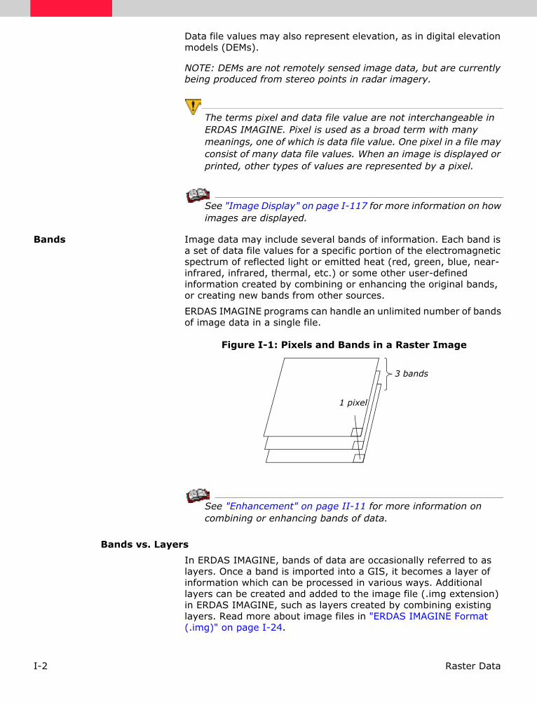
I-2 Raster Data

Data file values may also represent elevation, as in digital elevation models (DEMs).

NOTE: DEMs are not remotely sensed image data, but are currently being produced from stereo points in radar imagery.

The terms pixel and data file value are not interchangeable in ERDAS IMAGINE. Pixel is used as a broad term with many meanings, one of which is data file value. One pixel in a file may consist of many data file values. When an image is displayed or printed, other types of values are represented by a pixel.

See "Image Display" on page I-117 for more information on how images are displayed.

Bands Image data may include several bands of information. Each band is a set of data file values for a specific portion of the electromagnetic spectrum of reflected light or emitted heat (red, green, blue, near-infrared, infrared, thermal, etc.) or some other user-defined information created by combining or enhancing the original bands, or creating new bands from other sources.

ERDAS IMAGINE programs can handle an unlimited number of bands of image data in a single file.

Figure I-1: Pixels and Bands in a Raster Image

See "Enhancement" on page II-11 for more information on combining or enhancing bands of data.

Bands vs. Layers

In ERDAS IMAGINE, bands of data are occasionally referred to as layers. Once a band is imported into a GIS, it becomes a layer of information which can be processed in various ways. Additional layers can be created and added to the image file (.img extension) in ERDAS IMAGINE, such as layers created by combining existing layers. Read more about image files in "ERDAS IMAGINE Format (.img)" on page I-24.

1 pixel

3 bands

I-3Raster Data

Layers vs. Viewer Layers

The Viewer permits several images to be layered, in which case each image (including a multiband image) may be a layer.

Numeral Types

The range and the type of numbers used in a raster layer determine how the layer is displayed and processed. For example, a layer of elevation data with values ranging from -51.257 to 553.401 would be treated differently from a layer using only two values to show land and water.

The data file values in raster layers generally fall into these categories:

• Nominal data file values are simply categorized and named. The actual value used for each category has no inherent meaning—it is simply a class value. An example of a nominal raster layer would be a thematic layer showing tree species.

• Ordinal data are similar to nominal data, except that the file values put the classes in a rank or order. For example, a layer with classes numbered and named 1 - Good, 2 - Moderate, and 3 - Poor is an ordinal system.

• Interval data file values have an order, but the intervals between the values are also meaningful. Interval data measure some characteristic, such as elevation or degrees Fahrenheit, which does not necessarily have an absolute zero. (The difference between two values in interval data is meaningful.)

• Ratio data measure a condition that has a natural zero, such as electromagnetic radiation (as in most remotely sensed data), rainfall, or slope.

Nominal and ordinal data lend themselves to applications in which categories, or themes, are used. Therefore, these layers are sometimes called categorical or thematic.

Likewise, interval and ratio layers are more likely to measure a condition, causing the file values to represent continuous gradations across the layer. Such layers are called continuous.

Coordinate Systems The location of a pixel in a file or on a displayed or printed image is expressed using a coordinate system. In two-dimensional coordinate systems, locations are organized in a grid of columns and rows. Each location on the grid is expressed as a pair of coordinates known as X and Y. The X coordinate specifies the column of the grid, and the Y coordinate specifies the row. Image data organized into such a grid are known as raster data.

There are two basic coordinate systems used in ERDAS IMAGINE:

• file coordinates—indicate the location of a pixel within the image (data file)

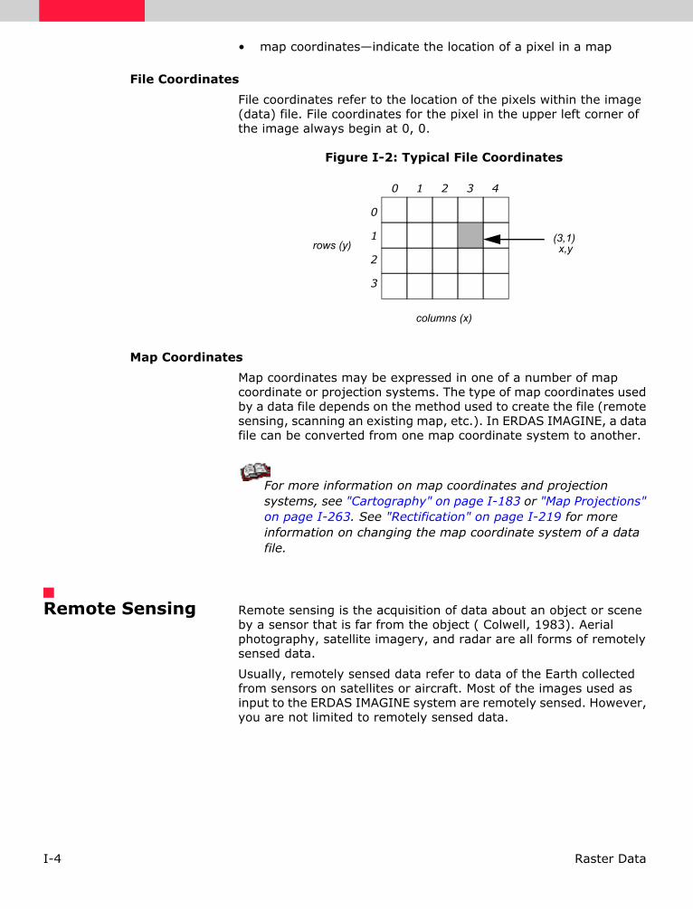
I-4 Raster Data

• map coordinates—indicate the location of a pixel in a map

File Coordinates

File coordinates refer to the location of the pixels within the image (data) file. File coordinates for the pixel in the upper left corner of the image always begin at 0, 0.

Figure I-2: Typical File Coordinates

Map Coordinates

Map coordinates may be expressed in one of a number of map coordinate or projection systems. The type of map coordinates used by a data file depends on the method used to create the file (remote sensing, scanning an existing map, etc.). In ERDAS IMAGINE, a data file can be converted from one map coordinate system to another.

For more information on map coordinates and projection systems, see "Cartography" on page I-183 or "Map Projections" on page I-263. See "Rectification" on page I-219 for more information on changing the map coordinate system of a data file.

Remote Sensing Remote sensing is the acquisition of data about an object or scene by a sensor that is far from the object ( Colwell, 1983). Aerial photography, satellite imagery, and radar are all forms of remotely sensed data.

Usually, remotely sensed data refer to data of the Earth collected from sensors on satellites or aircraft. Most of the images used as input to the ERDAS IMAGINE system are remotely sensed. However, you are not limited to remotely sensed data.

rows (y)(3,1)x,y

columns (x)

0

1

2

3

0 1 2 3 4

I-5Raster Data

This section is a brief introduction to remote sensing. There are many books available for more detailed information, including Colwell, 1983, Swain and Davis, 1978; and Slater, 1980 (see "Bibliography" on page II-317).

Electromagnetic Radiation Spectrum

The sensors on remote sensing platforms usually record electromagnetic radiation. Electromagnetic radiation (EMR) is energy transmitted through space in the form of electric and magnetic waves ( Star and Estes, 1990). Remote sensors are made up of detectors that record specific wavelengths of the electromagnetic spectrum. The electromagnetic spectrum is the range of electromagnetic radiation extending from cosmic waves to radio waves ("Jensen, 1996").

All types of land cover (rock types, water bodies, etc.) absorb a portion of the electromagnetic spectrum, giving a distinguishable signature of electromagnetic radiation. Armed with the knowledge of which wavelengths are absorbed by certain features and the intensity of the reflectance, you can analyze a remotely sensed image and make fairly accurate assumptions about the scene. "Figure I-3:" illustrates the electromagnetic spectrum ( Suits, 1983; Star and Estes, 1990).

Figure I-3: Electromagnetic Spectrum

SWIR and LWIR

The near-infrared and middle-infrared regions of the electromagnetic spectrum are sometimes referred to as the short wave infrared region (SWIR). This is to distinguish this area from the thermal or far infrared region, which is often referred to as the long wave infrared region (LWIR). The SWIR is characterized by reflected radiation whereas the LWIR is characterized by emitted radiation.

micrometers µm (one millionth of a meter)

0 1.0 2.0 3.0 4.0 5.0 6.0 7.0 8.0 9.0 10.0 11.0 12.0 13.0 14.0 15.0 16.0 17.0

Reflected Thermal

SWIR LWIR

Visible(0.4 - 0.7)

Blue (0.4 - 0.5)Green (0.5 - 0.6)Red (0.6 - 0.7)

Near-infrared(0.7 - 2.0)

Ultraviolet

Middle-infrared(2.0 - 5.0)

Far-infrared(8.0 - 15.0)

Radar

I-6 Raster Data

Absorption / Reflection Spectra

When radiation interacts with matter, some wavelengths are absorbed and others are reflected.To enhance features in image data, it is necessary to understand how vegetation, soils, water, and other land covers reflect and absorb radiation. The study of the absorption and reflection of EMR waves is called spectroscopy.

Spectroscopy

Most commercial sensors, with the exception of imaging radar sensors, are passive solar imaging sensors. Passive solar imaging sensors can only receive radiation waves; they cannot transmit radiation. (Imaging radar sensors are active sensors that emit a burst of microwave radiation and receive the backscattered radiation.)

The use of passive solar imaging sensors to characterize or identify a material of interest is based on the principles of spectroscopy. Therefore, to fully utilize a visible/infrared (VIS/IR) multispectral data set and properly apply enhancement algorithms, it is necessary to understand these basic principles. Spectroscopy reveals the:

• absorption spectra—the EMR wavelengths that are absorbed by specific materials of interest

• reflection spectra—the EMR wavelengths that are reflected by specific materials of interest

Absorption Spectra

Absorption is based on the molecular bonds in the (surface) material. Which wavelengths are absorbed depends upon the chemical composition and crystalline structure of the material. For pure compounds, these absorption bands are so specific that the SWIR region is often called an infrared fingerprint.

Atmospheric Absorption

In remote sensing, the sun is the radiation source for passive sensors. However, the sun does not emit the same amount of radiation at all wavelengths. "Figure I-4:" shows the solar irradiation curve, which is far from linear.

I-7Raster Data

Figure I-4: Sun Illumination Spectral Irradiance at the Earth’s Surface

Source: Modified from Chahine et al, 1983

Solar radiation must travel through the Earth’s atmosphere before it reaches the Earth’s surface. As it travels through the atmosphere, radiation is affected by four phenomena ( Elachi, 1987):

• absorption—the amount of radiation absorbed by the atmosphere

• scattering—the amount of radiation scattered away from the field of view by the atmosphere

• scattering source—divergent solar irradiation scattered into the field of view

• emission source—radiation re-emitted after absorption

00.0

Eλ Spec

tral

Irr

adia

nce

(W

m-2

m -1

)

3.01.5 2.72.42.11.81.20.90.60.3Wavelength µm

2500

2000

1500

1000

500

UV VIS INFRARED

Solar irradiation curve outside atmosphere

Solar irradiation curve at sea levelPeaks show absorption by H20, C02, and O3

I-8 Raster Data

Figure I-5: Factors Affecting Radiation

Source: Elachi, 1987

Absorption is not a linear phenomena—it is logarithmic with concentration ( Flaschka, 1969). In addition, the concentration of atmospheric gases, especially water vapor, is variable. The other major gases of importance are carbon dioxide (CO2) and ozone (O3), which can vary considerably around urban areas. Thus, the extent of atmospheric absorbance varies with humidity, elevation, proximity to (or downwind of) urban smog, and other factors.

Scattering is modeled as Rayleigh scattering with a commonly used algorithm that accounts for the scattering of short wavelength energy by the gas molecules in the atmosphere ( Pratt, 1991)—for example, ozone. Scattering is variable with both wavelength and atmospheric aerosols. Aerosols differ regionally (ocean vs. desert) and daily (for example, Los Angeles smog has different concentrations daily).

Scattering source and emission source may account for only 5% of the variance. These factors are minor, but they must be considered for accurate calculation. After interaction with the target material, the reflected radiation must travel back through the atmosphere and be subjected to these phenomena a second time to arrive at the satellite.

Absorption—the amount of

Scattering—the amount of radiation

Scattering Source—divergent solar

Emission Source—radiation

Radiation

radiation absorbed by theatmosphere

re-emitted after absorption

scattered away from the field of view

irradiations scattered into thefield of view

by the atmosphere

I-9Raster Data

The mathematical models that attempt to quantify the total atmospheric effect on the solar illumination are called radiative transfer equations. Some of the most commonly used are Lowtran ( Kneizys et al, 1988) and Modtran ( Berk et al, 1989).

See "Enhancement" on page II-11 for more information on atmospheric modeling.

Reflectance Spectra

After rigorously defining the incident radiation (solar irradiation at target), it is possible to study the interaction of the radiation with the target material. When an electromagnetic wave (solar illumination in this case) strikes a target surface, three interactions are possible ( Elachi, 1987):

• reflection

• transmission

• scattering

It is the reflected radiation, generally modeled as bidirectional reflectance ( Clark and Roush, 1984), that is measured by the remote sensor.

Remotely sensed data are made up of reflectance values. The resulting reflectance values translate into discrete digital numbers (or values) recorded by the sensing device. These gray scale values fit within a certain bit range (such as 0 to 255, which is 8-bit data) depending on the characteristics of the sensor.

Each satellite sensor detector is designed to record a specific portion of the electromagnetic spectrum. For example, Landsat Thematic Mapper (TM) band 1 records the 0.45 to 0.52 µm portion of the spectrum and is designed for water body penetration, making it useful for coastal water mapping. It is also useful for soil/vegetation discriminations, forest type mapping, and cultural features identification ( Lillesand and Kiefer, 1987).

The characteristics of each sensor provide the first level of constraints on how to approach the task of enhancing specific features, such as vegetation or urban areas. Therefore, when choosing an enhancement technique, one should pay close attention to the characteristics of the land cover types within the constraints imposed by the individual sensors.

I-10 Raster Data

The use of VIS/IR imagery for target discrimination, whether the target is mineral, vegetation, man-made, or even the atmosphere itself, is based on the reflectance spectrum of the material of interest (see "Figure I-6:" ). Every material has a characteristic spectrum based on the chemical composition of the material. When sunlight (the illumination source for VIS/IR imagery) strikes a target, certain wavelengths are absorbed by the chemical bonds; the rest are reflected back to the sensor. It is, in fact, the wavelengths that are not returned to the sensor that provide information about the imaged area.

Specific wavelengths are also absorbed by gases in the atmosphere (H2O vapor, CO2, O2, etc.). If the atmosphere absorbs a large percentage of the radiation, it becomes difficult or impossible to use that particular wavelength(s) to study the Earth. For the present Landsat and Systeme Pour l’observation de la Terre (SPOT) sensors, only the water vapor bands are considered strong enough to exclude the use of their spectral absorption region. "Figure I-6:" shows how Landsat TM bands 5 and 7 were carefully placed to avoid these regions. Absorption by other atmospheric gases was not extensive enough to eliminate the use of the spectral region for present day broad band sensors.

Figure I-6: Reflectance Spectra

100

80

60

40

20

0

Ref

lect

ance

, %

.4 .6 .8 1.0 1.2 1.4 1.6 1.8 2.0 2.2 2.4

Wavelength, µm

Vegetation (green)

Silt loam

Atmospheric

bands

4 5 6 7 Landsat MSS bands

1 2 3 4 5 7Landsat TM bands

Kaolinite

absorption

I-11Raster Data

Source: Modified from Fraser, 1986; Crist et al, 1986; Sabins, 1987

NOTE: This chart is for comparison purposes only. It is not meant to show actual values. The spectra are offset to better display the lines.

An inspection of the spectra reveals the theoretical basis of some of the indices in the ERDAS IMAGINE Image Interpreter. Consider the vegetation index TM4/TM3. It is readily apparent that for vegetation this value could be very large. For soils, the value could be much smaller, and for clay minerals, the value could be near zero. Conversely, when the clay ratio TM5/TM7 is considered, the opposite applies.

Hyperspectral Data

As remote sensing moves toward the use of more and narrower bands (for example, AVIRIS with 224 bands each only 10 nm wide), absorption by specific atmospheric gases must be considered. These multiband sensors are called hyperspectral sensors. As more and more of the incident radiation is absorbed by the atmosphere, the digital number (DN) values of that band get lower, eventually becoming useless—unless one is studying the atmosphere. Someone wanting to measure the atmospheric content of a specific gas could utilize the bands of specific absorption.

NOTE: Hyperspectral bands are generally measured in nanometers (nm).

"Figure I-6:" shows the spectral bandwidths of the channels for the Landsat sensors plotted above the absorption spectra of some common natural materials (kaolin clay, silty loam soil, and green vegetation). Note that while the spectra are continuous, the Landsat channels are segmented or discontinuous. We can still use the spectra in interpreting the Landsat data. For example, a Normalized Difference Vegetation Index (NDVI) ratio for the three would be very different and, therefore, could be used to discriminate between the three materials. Similarly, the ratio TM5/TM7 is commonly used to measure the concentration of clay minerals. Evaluation of the spectra shows why.

"Figure I-7:" shows detail of the absorption spectra of three clay minerals. Because of the wide bandpass (2080 to 2350 nm) of TM band 7, it is not possible to discern between these three minerals with the Landsat sensor. As mentioned, the AVIRIS hyperspectral sensor has a large number of approximately 10 nm wide bands. With the proper selection of band ratios, mineral identification becomes possible. With this data set, it would be possible to discriminate between these three clay minerals, again using band ratios. For example, a color composite image prepared from RGB = 2160nm/2190nm, 2220nm/2250nm, 2350nm/2488nm could produce a color-coded clay mineral image-map.

I-12 Raster Data

The commercial airborne multispectral scanners are used in a similar fashion. The Airborne Imaging Spectrometer from the Geophysical & Environmental Research Corp. (GER) has 79 bands in the UV, visible, SWIR, and thermal-infrared regions. The Airborne Multispectral Scanner Mk2 by Geoscan Pty, Ltd., has up to 52 bands in the visible, SWIR, and thermal-infrared regions. To properly utilize these hyperspectral sensors, you must understand the phenomenon involved and have some idea of the target materials being sought.

Figure I-7: Laboratory Spectra of Clay Minerals in the Infrared Region

Source: Modified from Sabins, 1987

NOTE: Spectra are offset vertically for clarity.

The characteristics of Landsat, AVIRIS, and other data types are discussed in "Raster and Vector Data Sources" on page I-49. See "Enhancement" on page II-11 for more information on the NDVI ratio.

2000 2200 2400 2600

Landsat TM band 7

2080 nm 2350 nm

Kaolinite

Montmorillonite

Illite

Ref

lect

ance

, %

Wavelength, nm

I-13Raster Data

Imaging Radar Data

Radar remote sensors can be broken into two broad categories: passive and active. The passive sensors record the very low intensity, microwave radiation naturally emitted by the Earth. Because of the very low intensity, these images have low spatial resolution (i.e., large pixel size).

It is the active sensors, termed imaging radar, that are introducing a new generation of satellite imagery to remote sensing. To produce an image, these satellites emit a directed beam of microwave energy at the target, and then collect the backscattered (reflected) radiation from the target scene. Because they must emit a powerful burst of energy, these satellites require large solar collectors and storage batteries. For this reason, they cannot operate continuously; some satellites are limited to 10 minutes of operation per hour.

The microwave energy emitted by an active radar sensor is coherent and defined by a narrow bandwidth. The following table summarizes the bandwidths used in remote sensing.

*Wavelengths commonly used in imaging radars are shown in parentheses.

A key element of a radar sensor is the antenna. For a given position in space, the resolution of the resultant image is a function of the antenna size. This is termed a real-aperture radar (RAR). At some point, it becomes impossible to make a large enough antenna to create the desired spatial resolution. To get around this problem, processing techniques have been developed which combine the signals received by the sensor as it travels over the target. Thus, the antenna is perceived to be as long as the sensor path during backscatter reception. This is termed a synthetic aperture and the sensor a synthetic aperture radar (SAR).

Table I-1: Bandwidths Used in Remote Sensing

Band Designation*

Wavelength (λ), cm

Frequency (υ), GHz

(109 cycles · sec-1)

Ka (0.86 cm) 0.8 to 1.1 40.0 to 26.5

K 1.1 to 1.7 26.5 to 18.0

Ku 1.7 to 2.4 18.0 to 12.5

X (3.0 cm, 3.2 cm) 2.4 to 3.8 12.5 to 8.0

C 3.8 to 7.5 8.0 to 4.0

S 7.5 to 15.0 4.0 to 2.0

L (23.5 cm, 25.0 cm) 15.0 to 30.0 2.0 to 1.0

P 30.0 to 100.0 1.0 to 0.3

I-14 Raster Data

The received signal is termed a phase history or echo hologram. It contains a time history of the radar signal over all the targets in the scene, and is itself a low resolution RAR image. In order to produce a high resolution image, this phase history is processed through a hardware/software system called an SAR processor. The SAR processor software requires operator input parameters, such as information about the sensor flight path and the radar sensor's characteristics, to process the raw signal data into an image. These input parameters depend on the desired result or intended application of the output imagery.

One of the most valuable advantages of imaging radar is that it creates images from its own energy source and therefore is not dependent on sunlight. Thus one can record uniform imagery any time of the day or night. In addition, the microwave frequencies at which imaging radars operate are largely unaffected by the atmosphere. This allows image collection through cloud cover or rain storms. However, the backscattered signal can be affected. Radar images collected during heavy rainfall are often seriously attenuated, which decreases the signal-to-noise ratio (SNR). In addition, the atmosphere does cause perturbations in the signal phase, which decreases resolution of output products, such as the SAR image or generated DEMs.

Resolution Resolution is a broad term commonly used to describe:

• the number of pixels you can display on a display device, or

• the area on the ground that a pixel represents in an image file.

These broad definitions are inadequate when describing remotely sensed data. Four distinct types of resolution must be considered:

• spectral—the specific wavelength intervals that a sensor can record

• spatial—the area on the ground represented by each pixel

• radiometric—the number of possible data file values in each band (indicated by the number of bits into which the recorded energy is divided)

• temporal—how often a sensor obtains imagery of a particular area

These four domains contain separate information that can be extracted from the raw data.

Spectral Resolution Spectral resolution refers to the specific wavelength intervals in the electromagnetic spectrum that a sensor can record ( Simonett et al, 1983). For example, band 1 of the Landsat TM sensor records energy between 0.45 and 0.52 µm in the visible part of the spectrum.

I-15Raster Data

Wide intervals in the electromagnetic spectrum are referred to as coarse spectral resolution, and narrow intervals are referred to as fine spectral resolution. For example, the SPOT panchromatic sensor is considered to have coarse spectral resolution because it records EMR between 0.51 and 0.73 µm. On the other hand, band 3 of the Landsat TM sensor has fine spectral resolution because it records EMR between 0.63 and 0.69 µm ( Jensen, 1996).

NOTE: The spectral resolution does not indicate how many levels the signal is broken into.

Spatial Resolution Spatial resolution is a measure of the smallest object that can be resolved by the sensor, or the area on the ground represented by each pixel ( Simonett et al, 1983). The finer the resolution, the lower the number. For instance, a spatial resolution of 79 meters is coarser than a spatial resolution of 10 meters.

Scale

The terms large-scale imagery and small-scale imagery often refer to spatial resolution. Scale is the ratio of distance on a map as related to the true distance on the ground ( Star and Estes, 1990).

Large-scale in remote sensing refers to imagery in which each pixel represents a small area on the ground, such as SPOT data, with a spatial resolution of 10 m or 20 m. Small scale refers to imagery in which each pixel represents a large area on the ground, such as Advanced Very High Resolution Radiometer (AVHRR) data, with a spatial resolution of 1.1 km.

This terminology is derived from the fraction used to represent the scale of the map, such as 1:50,000. Small-scale imagery is represented by a small fraction (one over a very large number). Large-scale imagery is represented by a larger fraction (one over a smaller number). Generally, anything smaller than 1:250,000 is considered small-scale imagery.

NOTE: Scale and spatial resolution are not always the same thing. An image always has the same spatial resolution, but it can be presented at different scales ( Simonett et al, 1983).

Instantaneous Field of View

Spatial resolution is also described as the instantaneous field of view (IFOV) of the sensor, although the IFOV is not always the same as the area represented by each pixel. The IFOV is a measure of the area viewed by a single detector in a given instant in time ( Star and Estes, 1990). For example, Landsat MSS data have an IFOV of 79 × 79 meters, but there is an overlap of 11.5 meters in each pass of the scanner, so the actual area represented by each pixel is 56.5 × 79 meters (usually rounded to 57 × 79 meters).

Even though the IFOV is not the same as the spatial resolution, it is important to know the number of pixels into which the total field of view for the image is broken. Objects smaller than the stated pixel size may still be detectable in the image if they contrast with the background, such as roads, drainage patterns, etc.

I-16 Raster Data

On the other hand, objects the same size as the stated pixel size (or larger) may not be detectable if there are brighter or more dominant objects nearby. In "Figure I-8:" , a house sits in the middle of four pixels. If the house has a reflectance similar to its surroundings, the data file values for each of these pixels reflect the area around the house, not the house itself, since the house does not dominate any one of the four pixels. However, if the house has a significantly different reflectance than its surroundings, it may still be detectable.

Figure I-8: IFOV

Radiometric Resolution Radiometric resolution refers to the dynamic range, or number of possible data file values in each band. This is referred to by the number of bits into which the recorded energy is divided.

For instance, in 8-bit data, the data file values range from 0 to 255 for each pixel, but in 7-bit data, the data file values for each pixel range from 0 to 128.

In "Figure I-9:" , 8-bit and 7-bit data are illustrated. The sensor measures the EMR in its range. The total intensity of the energy from 0 to the maximum amount the sensor measures is broken down into 256 brightness values for 8-bit data, and 128 brightness values for 7-bit data.

20 m

20 m

house

20 m

20 m

I-17Raster Data

Figure I-9: Brightness Values

Temporal Resolution Temporal resolution refers to how often a sensor obtains imagery of a particular area. For example, the Landsat satellite can view the same area of the globe once every 16 days. SPOT, on the other hand, can revisit the same area every three days.

NOTE: Temporal resolution is an important factor to consider in change detection studies.

"Figure I-10:" illustrates all four types of resolution:

Figure I-10: Landsat TM—Band 2 (Four Types of Resolution)

Source: EOSAT

Data Correction There are several types of errors that can be manifested in remotely sensed data. Among these are line dropout and striping. These errors can be corrected to an extent in GIS by radiometric and geometric correction functions.

NOTE: Radiometric errors are usually already corrected in data from EOSAT or SPOT.

8-bit

0

7-bit

0 1 2 3 4 5 122 123 124 125 126 127

0 max. intensity

244 25524911 109876543210

max. intensity

Spatial Resolution:

1 pixel = 79 m ¥ 79 m

Temporal Resolution: same area viewed every 16 days

79 m79 m

Day 1

Day 17

Day 31

Radiometric Resolution:

8-bit (0 - 255)

Spectral Resolution:

0.52 - 0.60 µm

I-18 Raster Data

See "Enhancement" on page II-11 for more information on radiometric and geometric correction.

Line Dropout Line dropout occurs when a detector either completely fails to function or becomes temporarily saturated during a scan (like the effect of a camera flash on a human retina). The result is a line or partial line of data with higher data file values, creating a horizontal streak until the detector(s) recovers, if it recovers.

Line dropout is usually corrected by replacing the bad line with a line of estimated data file values. The estimated line is based on the lines above and below it.

You can correct line dropout using the 5 × 5 Median Filter from the Radar Speckle Suppression function. The Convolution and Focal Analysis functions in the ERDAS IMAGINE Image Interpreter also corrects for line dropout.

Striping Striping or banding occurs if a detector goes out of adjustment—that is, it provides readings consistently greater than or less than the other detectors for the same band over the same ground cover.

Use ERDAS IMAGINE Image Interpreter or ERDAS IMAGINE Spatial Modeler for implementing algorithms to eliminate striping. The ERDAS IMAGINE Spatial Modeler editing capabilities allow you to adapt the algorithms to best address the data.

Data Storage Image data can be stored on a variety of media—tapes, CD-ROMs, or floppy diskettes, for example—but how the data are stored (e.g., structure) is more important than on what they are stored.

All computer data are in binary format. The basic unit of binary data is a bit. A bit can have two possible values—0 and 1, or “off” and “on” respectively. A set of bits, however, can have many more values, depending on the number of bits used. The number of values that can be expressed by a set of bits is 2 to the power of the number of bits used.

A byte is 8 bits of data. Generally, file size and disk space are referred to by number of bytes. For example, a PC may have 640 kilobytes (1,024 bytes = 1 kilobyte) of RAM (random access memory), or a file may need 55,698 bytes of disk space. A megabyte (Mb) is about one million bytes. A gigabyte (Gb) is about one billion bytes.

Storage Formats Image data can be arranged in several ways on a tape or other media. The most common storage formats are:

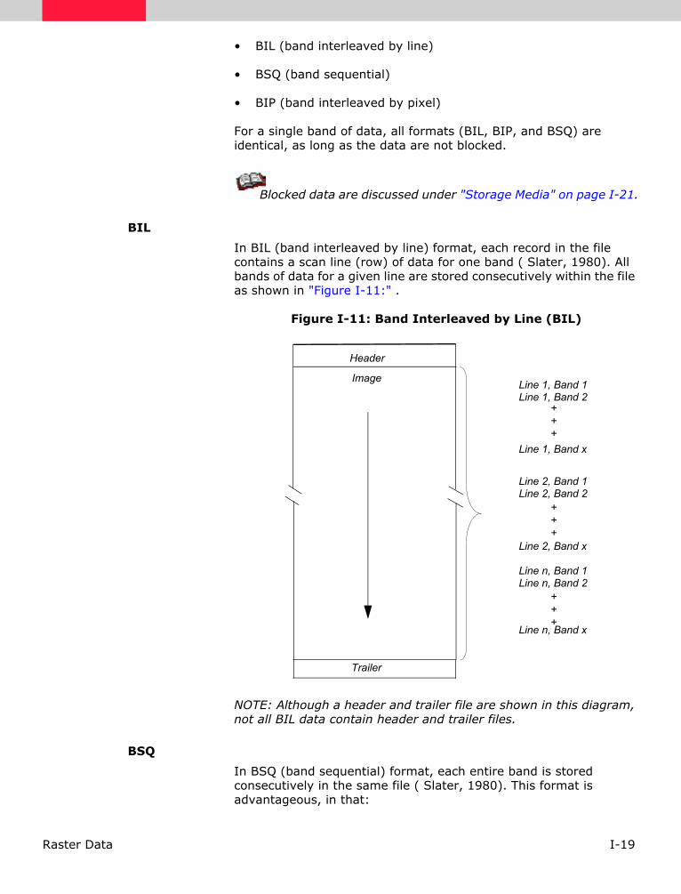
I-19Raster Data

• BIL (band interleaved by line)

• BSQ (band sequential)

• BIP (band interleaved by pixel)

For a single band of data, all formats (BIL, BIP, and BSQ) are identical, as long as the data are not blocked.

Blocked data are discussed under "Storage Media" on page I-21.

BIL

In BIL (band interleaved by line) format, each record in the file contains a scan line (row) of data for one band ( Slater, 1980). All bands of data for a given line are stored consecutively within the file as shown in "Figure I-11:" .

Figure I-11: Band Interleaved by Line (BIL)

NOTE: Although a header and trailer file are shown in this diagram, not all BIL data contain header and trailer files.

BSQ

In BSQ (band sequential) format, each entire band is stored consecutively in the same file ( Slater, 1980). This format is advantageous, in that:

Header

Trailer

Image Line 1, Band 1Line 1, Band 2

+++

Line 1, Band x

Line 2, Band 1Line 2, Band 2

+++

Line 2, Band x

Line n, Band 1Line n, Band 2

+++

Line n, Band x

I-20 Raster Data

• one band can be read and viewed easily, and

• multiple bands can be easily loaded in any order.

Figure I-12: Band Sequential (BSQ)

Landsat TM data are stored in a type of BSQ format known as fast format. Fast format data have the following characteristics:

• Files are not split between tapes. If a band starts on the first tape, it ends on the first tape.

• An end-of-file (EOF) marker follows each band.

• An end-of-volume marker marks the end of each volume (tape). An end-of-volume marker consists of three end-of-file markers.

• There is one header file per tape.

• There are no header records preceding the image data.

• Regular products (not geocoded) are normally unblocked. Geocoded products are normally blocked (EOSAT).

ERDAS IMAGINE imports all of the header and image file information.

Header File(s)

end-of-file

end-of-file

Trailer File(s)

Image FileBand 1

Image File

Band 2

Image FileBand x

Line 1, Band 1Line 2, Band 2Line 3, Band 3

+++

Line n, Band 1

Line 1, Band 2Line 2, Band 2Line 3, Band 2

+++

Line n, Band 2

Line 1, Band xLine 2, Band xLine 3, Band x

+++

Line n, Band x

I-21Raster Data

See "Geocoded Data" on page I-29 for more information on geocoded data.

BIP

In BIP (band interleaved by pixel) format, the values for each band are ordered within a given pixel. The pixels are arranged sequentially on the tape ( Slater, 1980). The sequence for BIP format is:

Pixel 1, Band 1

Pixel 1, Band 2

Pixel 1, Band 3

.

.

.Pixel 2, Band 1

Pixel 2, Band 2

Pixel 2, Band 3

.

.

.

Storage Media Today, most raster data are available on a variety of storage media to meet the needs of users, depending on the system hardware and devices available. When ordering data, it is sometimes possible to select the type of media preferred. The most common forms of storage media are discussed in the following section:

• 9-track tape

• 4 mm tape

• 8 mm tape

• 1/4” cartridge tape

• CD-ROM/optical disk

Other types of storage media are:

• floppy disk (3.5” or 5.25”)

• film, photograph, or paper

• videotape

I-22 Raster Data

Tape

The data on a tape can be divided into logical records and physical records. A record is the basic storage unit on a tape.

• A logical record is a series of bytes that form a unit. For example, all the data for one line of an image may form a logical record.

• A physical record is a consecutive series of bytes on a magnetic tape, followed by a gap, or blank space, on the tape.

Blocked Data

For reasons of efficiency, data can be blocked to fit more on a tape. Blocked data are sequenced so that there are more logical records in each physical record. The number of logical records in each physical record is the blocking factor. For instance, a record may contain 28,000 bytes, but only 4000 columns due to a blocking factor of 7.

Tape Contents

Tapes are available in a variety of sizes and storage capacities. To obtain information about the data on a particular tape, read the tape label or box, or read the header file. Often, there is limited information on the outside of the tape. Therefore, it may be necessary to read the header files on each tape for specific information, such as:

• number of tapes that hold the data set

• number of columns (in pixels)

• number of rows (in pixels)

• data storage format—BIL, BSQ, BIP

• pixel depth—4-bit, 8-bit, 10-bit, 12-bit, 16-bit

• number of bands

• blocking factor

• number of header files and header records

4 mm Tapes

The 4 mm tape is a relative newcomer in the world of GIS. This tape is a mere 2” × .75” in size, but it can hold up to 2 Gb of data. This petite cassette offers an obvious shipping and storage advantage because of its size.

I-23Raster Data

8 mm Tapes

The 8 mm tape offers the advantage of storing vast amounts of data. Tapes are available in 5 and 10 Gb storage capacities (although some tape drives cannot handle the 10 Gb size). The 8 mm tape is a 2.5” × 4” cassette, which makes it easy to ship and handle.

1/4” Cartridge Tapes

This tape format falls between the 8 mm and 9-track in physical size and storage capacity. The tape is approximately 4” × 6” in size and stores up to 150 Mb of data.

9-Track Tapes

A 9-track tape is an older format that was the standard for two decades. It is a large circular tape approximately 10” in diameter. It requires a 9-track tape drive as a peripheral device for retrieving data. The size and storage capability make 9-track less convenient than 8 mm or 1/4” tapes. However, 9-track tapes are still widely used.

A single 9-track tape may be referred to as a volume. The complete set of tapes that contains one image is referred to as a volume set.

The storage format of a 9-track tape in binary format is described by the number of bits per inch, bpi, on the tape. The tapes most commonly used have either 1600 or 6250 bpi. The number of bits per inch on a tape is also referred to as the tape density. Depending on the length of the tape, 9-tracks can store between 120-150 Mb of data.

CD-ROM

Data such as ADRG and Digital Line Graphs (DLG) are most often available on CD-ROM, although many types of data can be requested in CD-ROM format. A CD-ROM is an optical read-only storage device which can be read with a CD player. CD-ROMs offer the advantage of storing large amounts of data in a small, compact device. Up to 644 Mb can be stored on a CD-ROM. Also, since this device is read-only, it protects the data from accidentally being overwritten, erased, or changed from its original integrity. This is the most stable of the current media storage types and data stored on CD-ROM are expected to last for decades without degradation.

Calculating Disk Space To calculate the amount of disk space a raster file requires on an ERDAS IMAGINE system, use the following formula:

x y× b×( )( n×[ ) ] 1.4× output file size=

I-24 Raster Data

Where:

y = rows

x = columns

b = number of bytes per pixel

n = number of bands

1.4 adds 30% to the file size for pyramid layers and 10% for miscellaneous adjustments, such as histograms, lookup tables, etc.

NOTE: This output file size is approximate. See "Pyramid Layers" on page I-134 for more information.

For example, to load a 3 band, 16-bit file with 500 rows and 500 columns, about 2,100,000 bytes of disk space is needed.

Bytes Per Pixel

The number of bytes per pixel is listed below:

4-bit data: .5

8-bit data: 1.0

16-bit data: 2.0

NOTE: On the PC, disk space is shown in bytes. On the workstation, disk space is shown as kilobytes (1,024 bytes).

ERDAS IMAGINE Format (.img)

In ERDAS IMAGINE, file name extensions identify the file type. When data are imported into ERDAS IMAGINE, they are converted to the ERDAS IMAGINE file format and stored in image files. ERDAS IMAGINE image files (.img) can contain two types of raster layers:

• thematic

• continuous

An image file can store a combination of thematic and continuous layers, or just one type.

Figure I-13: Image Files Store Raster Layers

500 500×( ) 2×( ) 3×[ ] 1.4× 2 100 000, ,= or 2.1 Mb

Image File (.img)

Raster Layer(s)

Thematic Raster Layer(s) Continuous Raster Layer(s)

I-25Raster Data

ERDAS Version 7.5 Users

For Version 7.5 users, when importing a GIS file from Version 7.5, it becomes an image file with one thematic raster layer. When importing a LAN file, each band becomes a continuous raster layer within an image file.

Thematic Raster Layer

Thematic data are raster layers that contain qualitative, categorical information about an area. A thematic layer is contained within an image file. Thematic layers lend themselves to applications in which categories or themes are used. Thematic raster layers are used to represent data measured on a nominal or ordinal scale, such as:

• soils

• land use

• land cover

• roads

• hydrology

NOTE: Thematic raster layers are displayed as pseudo color layers.

Figure I-14: Example of a Thematic Raster Layer

See "Image Display" on page I-117 for information on displaying thematic raster layers.

soils

I-26 Raster Data

Continuous Raster Layer

Continuous data are raster layers that contain quantitative (measuring a characteristic on an interval or ratio scale) and related, continuous values. Continuous raster layers can be multiband (e.g., Landsat TM data) or single band (e.g., SPOT panchromatic data). The following types of data are examples of continuous raster layers:

• Landsat

• SPOT

• digitized (scanned) aerial photograph

• DEM

• slope

• temperature

NOTE: Continuous raster layers can be displayed as either a gray scale raster layer or a true color raster layer.

Figure I-15: Examples of Continuous Raster Layers

Tiled Data

Data in the .img format are tiled data. Tiled data are stored in tiles that can be set to any size.

The default tile size for image files is 64 × 64 pixels.

Image File Contents

The image files contain the following additional information about the data:

• the data file values

Landsat TM DEM

I-27Raster Data

• statistics

• lookup tables

• map coordinates

• map projection

This additional information can be viewed using the Image Information function located on the Viewer’s tool bar.

Statistics

In ERDAS IMAGINE, the file statistics are generated from the data file values in the layer and incorporated into the image file. This statistical information is used to create many program defaults, and helps you make processing decisions.

Pyramid Layers

Sometimes a large image takes longer than normal to display in the Viewer. The pyramid layer option enables you to display large images faster. Pyramid layers are image layers which are successively reduced by the power of 2 and resampled.

The Pyramid Layer option is available in the Image Information function located on the Viewer’s tool bar and, from the Import function.

See "Image Display" on page I-117 for more information on pyramid layers. See the On-Line Help for detailed information on ERDAS IMAGINE file formats.

Image File Organization

Data are easy to locate if the data files are well organized. Well organized files also make data more accessible to anyone who uses the system. Using consistent naming conventions and the ERDAS IMAGINE Image Catalog helps keep image files well organized and accessible.

I-28 Raster Data

Consistent Naming Convention

Many processes create an output file, and every time a file is created, it is necessary to assign a file name. The name that is used can either cause confusion about the process that has taken place, or it can clarify and give direction. For example, if the name of the output file is image.img, it is difficult to determine the contents of the file. On the other hand, if a standard nomenclature is developed in which the file name refers to a process or contents of the file, it is possible to determine the progress of a project and contents of a file by examining the directory.

Develop a naming convention that is based on the contents of the file. This helps everyone involved know what the file contains. For example, in a project to create a map composition for Lake Lanier, a directory for the files may look similar to the one below:

lanierTM.imglanierSPOT.imglanierSymbols.ovrlanierlegends.map.ovrlanierScalebars.map.ovrlanier.maplanier.pltlanier.gcclanierUTM.img

From this listing, one can make some educated guesses about the contents of each file based on naming conventions used. For example, lanierTM.img is probably a Landsat TM scene of Lake Lanier. The file lanier.map is probably a map composition that has map frames with lanierTM.img and lanierSPOT.img data in them. The file lanierUTM.img was probably created when lanierTM.img was rectified to a UTM map projection.

Keeping Track of Image Files

Using a database to store information about images enables you to track image files (.img) without having to know the name or location of the file. The database can be queried for specific parameters (e.g., size, type, map projection) and the database returns a list of image files that match the search criteria. This file information helps to quickly determine which image(s) to use, where it is located, and its ancillary data. An image database is especially helpful when there are many image files and even many on-going projects. For example, you could use the database to search for all of the image files of Georgia that have a UTM map projection.

Use the ERDAS IMAGINE Image Catalog to track and store information for image files (.img) that are imported and created in ERDAS IMAGINE.

NOTE: All information in the Image Catalog database, except archive information, is extracted from the image file header. Therefore, if this information is modified in the Image Information utility, it is necessary to recatalog the image in order to update the information in the Image Catalog database.

I-29Raster Data

ERDAS IMAGINE Image Catalog

The ERDAS IMAGINE Image Catalog database is designed to serve as a library and information management system for image files (.img) that are imported and created in ERDAS IMAGINE. The information for the image files is displayed in the Image Catalog CellArray™. This CellArray enables you to view all of the ancillary data for the image files in the database. When records are queried based on specific criteria, the image files that match the criteria are highlighted in the CellArray. It is also possible to graphically view the coverage of the selected image files on a map in a canvas window.

When it is necessary to store some data on a tape, the ERDAS IMAGINE Image Catalog database enables you to archive image files to external devices. The Image Catalog CellArray shows which tape the image file is stored on, and the file can be easily retrieved from the tape device to a designated disk directory. The archived image files are copies of the files on disk—nothing is removed from the disk. Once the file is archived, it can be removed from the disk, if you like.

Geocoded Data Geocoding, also known as georeferencing, is the geographical registration or coding of the pixels in an image. Geocoded data are images that have been rectified to a particular map projection and pixel size.

Raw, remotely-sensed image data are gathered by a sensor on a platform, such as an aircraft or satellite. In this raw form, the image data are not referenced to a map projection. Rectification is the process of projecting the data onto a plane and making them conform to a map projection system.

It is possible to geocode raw image data with the ERDAS IMAGINE rectification tools. Geocoded data are also available from Space Imaging EOSAT and SPOT.

See"Map Projections" on page I-263 for detailed information on the different projections available. See "Rectification" on page I-219 for information on geocoding raw imagery with ERDAS IMAGINE.

Using Image Data in GIS

ERDAS IMAGINE provides many tools designed to extract the necessary information from the images in a database. The following chapters in this book describe many of these processes.

This section briefly describes some basic image file techniques that may be useful for any application.

Subsetting and Mosaicking

Within ERDAS IMAGINE, there are options available to make additional image files from those acquired from EOSAT, SPOT, etc. These options involve combining files, mosaicking, and subsetting.

I-30 Raster Data

ERDAS IMAGINE programs allow image data with an unlimited number of bands, but the most common satellite data types—Landsat and SPOT—have seven or fewer bands. Image files can be created with more than seven bands.

It may be useful to combine data from two different dates into one file. This is called multitemporal imagery. For example, a user may want to combine Landsat TM from one date with TM data from a later date, then perform a classification based on the combined data. This is particularly useful for change detection studies.

You can also incorporate elevation data into an existing image file as another band, or create new bands through various enhancement techniques.

To combine two or more image files, each file must be georeferenced to the same coordinate system, or to each other. See "Rectification" on page I-219 for information on georeferencing images.

Subset

Subsetting refers to breaking out a portion of a large file into one or more smaller files. Often, image files contain areas much larger than a particular study area. In these cases, it is helpful to reduce the size of the image file to include only the area of interest (AOI). This not only eliminates the extraneous data in the file, but it speeds up processing due to the smaller amount of data to process. This can be important when dealing with multiband data.

The ERDAS IMAGINE Import option often lets you define a subset area of an image to preview or import. You can also use the Subset option from ERDAS IMAGINE Image Interpreter to define a subset area.

Mosaic

On the other hand, the study area in which you are interested may span several image files. In this case, it is necessary to combine the images to create one large file. This is called mosaicking.

To create a mosaicked image, use the Mosaic Images option from the Data Preparation menu.

Enhancement Image enhancement is the process of making an image more interpretable for a particular application ( Faust, 1989). Enhancement can make important features of raw, remotely sensed data and aerial photographs more interpretable to the human eye. Enhancement techniques are often used instead of classification for extracting useful information from images.

I-31Raster Data

There are many enhancement techniques available. They range in complexity from a simple contrast stretch, where the original data file values are stretched to fit the range of the display device, to principal components analysis, where the number of image file bands can be reduced and new bands created to account for the most variance in the data.

See "Enhancement" on page II-11 for more information on enhancement techniques.

Multispectral Classification

Image data are often used to create thematic files through multispectral classification. This entails using spectral pattern recognition to identify groups of pixels that represent a common characteristic of the scene, such as soil type or vegetation.

See "Classification" on page II-99 for a detailed explanation of classification procedures.

Editing Raster Data

ERDAS IMAGINE provides raster editing tools for editing the data values of thematic and continuous raster data. This is primarily a correction mechanism that enables you to correct bad data values which produce noise, such as spikes and holes in imagery. The raster editing functions can be applied to the entire image or a user-selected area of interest (AOI).

With raster editing, data values in thematic data can also be recoded according to class. Recoding is a function that reassigns data values to a region or to an entire class of pixels.

See "Geographic Information Systems" on page I-145 for information about recoding data. See "Enhancement" on page II-11 for information about reducing data noise using spatial filtering.

The ERDAS IMAGINE raster editing functions allow the use of focal and global spatial modeling functions for computing the values to replace noisy pixels or areas in continuous or thematic data.

Focal operations are filters that calculate the replacement value based on a window (3 × 3, 5 × 5, etc.), and replace the pixel of interest with the replacement value. Therefore this function affects one pixel at a time, and the number of surrounding pixels that influence the value is determined by the size of the moving window.

Global operations calculate the replacement value for an entire area rather than affecting one pixel at a time. These functions, specifically the Majority option, are more applicable to thematic data.

I-32 Raster Data

See the ERDAS IMAGINE On-Line Help for information about using and selecting AOIs.

The raster editing tools are available in the Viewer.

Editing Continuous (Athematic) Data

Editing DEMs

DEMs occasionally contain spurious pixels or bad data. These spikes, holes, and other noises caused by automatic DEM extraction can be corrected by editing the raster data values and replacing them with meaningful values. This discussion of raster editing focuses on DEM editing.

The ERDAS IMAGINE Raster Editing functionality was originally designed to edit DEMs, but it can also be used with images of other continuous data sources, such as radar, SPOT, Landsat, and digitized photographs.

When editing continuous raster data, you can modify or replace original pixel values with the following:

• a constant value—enter a known constant value for areas such as lakes.

• the average of the buffering pixels—replace the original pixel value with the average of the pixels in a specified buffer area around the AOI. This is used where the constant values of the AOI are not known, but the area is flat or homogeneous with little variation (for example, a lake).

• the original data value plus a constant value—add a negative constant value to the original data values to compensate for the height of trees and other vertical features in the DEM. This technique is commonly used in forested areas.

• spatial filtering—filter data values to eliminate noise such as spikes or holes in the data.

• interpolation techniques (discussed below).

Interpolation Techniques While the previously listed raster editing techniques are perfectly suitable for some applications, the following interpolation techniques provide the best methods for raster editing:

• 2-D polynomial—surface approximation

I-33Raster Data

• multisurface functions—with least squares prediction

• distance weighting

Each pixel’s data value is interpolated from the reference points in the data file. These interpolation techniques are described below:

2-D Polynomial

This interpolation technique provides faster interpolation calculations than distance weighting and multisurface functions. The following equation is used:

V = a0 + a1x + a2y + a2x2 + a4xy + a5y2 +. . .

Where:

V = data value (elevation value for DEM)

a = polynomial coefficients

x = x coordinate

y = y coordinate

Multisurface Functions

The multisurface technique provides the most accurate results for editing DEMs that have been created through automatic extraction. The following equation is used:

Where:

V = output data value (elevation value for DEM)

Wi = coefficients which are derived by the least squares method

Qi = distance-related kernels which are actually interpretable as continuous single value surfaces

Source: Wang, Z., 1990

Distance Weighting

The weighting function determines how the output data values are interpolated from a set of reference data points. For each pixel, the values of all reference points are weighted by a value corresponding with the distance between each point and the pixel.

The weighting function used in ERDAS IMAGINE is:

V WiQi∑=

W SD---- 1–

2=

I-34 Raster Data

Where:

S = normalization factor

D = distance from output data point and reference point

The value for any given pixel is calculated by taking the sum of weighting factors for all reference points multiplied by the data values of those points, and dividing by the sum of the weighting factors:

Where:

V = output data value (elevation value for DEM)

i = ith reference point

Wi = weighting factor of point i

Vi = data value of point i

n = number of reference points

Source: Wang, Z., 1990

V

Wi Vi×

i 1=

n

∑

Wi

i 1=

n

∑

----------------------------=

I-35Vector Data

Vector Data

Introduction ERDAS IMAGINE is designed to integrate two data types, raster and vector, into one system. While the previous chapter explored the characteristics of raster data, this chapter is focused on vector data. The vector data structure in ERDAS IMAGINE is based on the ArcInfo data model (developed by ESRI, Inc.). This chapter describes vector data, attribute information, and symbolization.

You do not need ArcInfo software or an ArcInfo license to use the vector capabilities in ERDAS IMAGINE. Since the ArcInfo data model is used in ERDAS IMAGINE, you can use ArcInfo coverages directly without importing them.

See "Geographic Information Systems" on page I-145 for information on editing vector layers and using vector data in a GIS.

Vector data consist of:

• points

• lines

• polygons

Each is illustrated in Figure I-16.

Figure I-16: Vector Elements

Points A point is represented by a single x, y coordinate pair. Points can represent the location of a geographic feature or a point that has no area, such as a mountain peak. Label points are also used to identify polygons (see Figure I-17).

node

node

vertices

polygons

label point

line

points

I-36 Vector Data

Lines A line (polyline) is a set of line segments and represents a linear geographic feature, such as a river, road, or utility line. Lines can also represent nongeographical boundaries, such as voting districts, school zones, contour lines, etc.

Polygons A polygon is a closed line or closed set of lines defining a homogeneous area, such as soil type, land use, or water body. Polygons can also be used to represent nongeographical features, such as wildlife habitats, state borders, commercial districts, etc. Polygons also contain label points that identify the polygon. The label point links the polygon to its attributes.

Vertex The points that define a line are vertices. A vertex is a point that defines an element, such as the endpoint of a line segment or a location in a polygon where the line segment defining the polygon changes direction. The ending points of a line are called nodes. Each line has two nodes: a from-node and a to-node. The from-node is the first vertex in a line. The to-node is the last vertex in a line. Lines join other lines only at nodes. A series of lines in which the from-node of the first line joins the to-node of the last line is a polygon.

Figure I-17: Vertices

In Figure I-17, the line and the polygon are each defined by three vertices.

Coordinates Vector data are expressed by the coordinates of vertices. The vertices that define each element are referenced with x, y, or Cartesian, coordinates. In some instances, those coordinates may be inches [as in some computer-aided design (CAD) applications], but often the coordinates are map coordinates, such as State Plane, Universal Transverse Mercator (UTM), or Lambert Conformal Conic. Vector data digitized from an ungeoreferenced image are expressed in file coordinates.

Tics

Vector layers are referenced to coordinates or a map projection system using tic files that contain geographic control points for the layer. Every vector layer must have a tic file. Tics are not topologically linked to other features in the layer and do not have descriptive data associated with them.

line polygon

vertices

label point

I-37Vector Data

Vector Layers Although it is possible to have points, lines, and polygons in a single layer, a layer typically consists of one type of feature. It is possible to have one vector layer for streams (lines) and another layer for parcels (polygons). A vector layer is defined as a set of features where each feature has a location (defined by coordinates and topological pointers to other features) and, possibly attributes (defined as a set of named items or variables) (ESRI 1989). Vector layers contain both the vector features (points, lines, polygons) and the attribute information.

Usually, vector layers are also divided by the type of information they represent. This enables the user to isolate data into themes, similar to the themes used in raster layers. Political districts and soil types would probably be in separate layers, even though both are represented with polygons. If the project requires that the coincidence of features in two or more layers be studied, the user can overlay them or create a new layer.

See "Geographic Information Systems" on page I-145 for more information about analyzing vector layers.

Topology The spatial relationships between features in a vector layer are defined using topology. In topological vector data, a mathematical procedure is used to define connections between features, identify adjacent polygons, and define a feature as a set of other features (e.g., a polygon is made of connecting lines) ( Environmental Systems Research Institute, 1990).

Topology is not automatically created when a vector layer is created. It must be added later using specific functions. Topology must be updated after a layer is edited also.

"Digitizing" on page I-42 describes how topology is created for a new or edited vector layer.

Vector Files As mentioned above, the ERDAS IMAGINE vector structure is based on the ArcInfo data model used for ARC coverages. This georelational data model is actually a set of files using the computer’s operating system for file management and input/output. An ERDAS IMAGINE vector layer is stored in subdirectories on the disk. Vector data are represented by a set of logical tables of information, stored as files within the subdirectory. These files may serve the following purposes:

• define features

• provide feature attributes

• cross-reference feature definition files

• provide descriptive information for the coverage as a whole

I-38 Vector Data

A workspace is a location that contains one or more vector layers. Workspaces provide a convenient means for organizing layers into related groups. They also provide a place for the storage of tabular data not directly tied to a particular layer. Each workspace is completely independent. It is possible to have an unlimited number of workspaces and an unlimited number of vector layers in a workspace. Table I-2, “Description of File Types” summarizes the types of files that are used to make up vector layers.

Figure I-18 illustrates how a typical vector workspace is set up ( Environmental Systems Research Institute, 1992).

Figure I-18: Workspace Structure

Table I-2: Description of File Types

File Type File Description

Feature Definition Files

ARC Line coordinates and topology

CNT Polygon centroid coordinates

LAB Label point coordinates and topology

TIC Tic coordinates

Feature Attribute Files

AAT Line (arc) attribute table

PAT Polygon or point attribute table

Feature Cross-Reference File

PAL Polygon/line/node cross-reference file

Layer Description Files

BND Coordinate extremes

LOG Layer history file

PRJ Coordinate definition file

TOL Layer tolerance file

georgia

parcels testdata

demo INFO roads streets

I-39Vector Data

Because vector layers are stored in directories rather than in simple files, you MUST use the utilities provided in ERDAS IMAGINE to copy and rename them. A utility is also provided to update path names that are no longer correct due to the use of regular system commands on vector layers.

See the ESRI documentation for more detailed information about the different vector files.

Attribute Information

Along with points, lines, and polygons, a vector layer can have a wealth of associated descriptive, or attribute, information associated with it. Attribute information is displayed in CellArrays. This is the same information that is stored in the INFO database of ArcInfo. Some attributes are automatically generated when the layer is created. Custom fields can be added to each attribute table. Attribute fields can contain numerical or character data.

The attributes for a roads layer may look similar to the example in Figure I-19. You can select features in the layer based on the attribute information. Likewise, when a row is selected in the attribute CellArray, that feature is highlighted in the Viewer.

Figure I-19: Attribute CellArray

Using Imported Attribute Data

When external data types are imported into ERDAS IMAGINE, only the required attribute information is imported into the attribute tables (AAT and PAT files) of the new vector layer. The rest of the attribute information is written to one of the following INFO files:

• <layer name>.ACODE—arc attribute information

• <layer name>.PCODE—polygon attribute information

I-40 Vector Data

• <layer name>.XCODE—point attribute information

To utilize all of this attribute information, the INFO files can be merged into the PAT and AAT files. Once this attribute information has been merged, it can be viewed in CellArrays and edited as desired. This new information can then be exported back to its original format.

The complete path of the file must be specified when establishing an INFO file name in a Viewer application, such as exporting attributes or merging attributes, as shown in the following example:

/georgia/parcels/info!arc!parcels.pcode

Use the Attributes option in the Viewer to view and manipulate vector attribute data, including merging and exporting. (The Raster Attribute Editor is for raster attributes only and cannot be used to edit vector attributes.)

See the ERDAS IMAGINE On-Line Help for more information about using CellArrays.

Displaying Vector Data

Vector data are displayed in Viewers, as are other data types in ERDAS IMAGINE. You can display a single vector layer, overlay several layers in one Viewer, or display a vector layer(s) over a raster layer(s).

In layers that contain more than one feature (a combination of points, lines, and polygons), you can select which features to display. For example, if you are studying parcels, you may want to display only the polygons in a layer that also contains street centerlines (lines).

Color Schemes Vector data are usually assigned class values in the same manner as the pixels in a thematic raster file. These class values correspond to different colors on the display screen. As with a pseudo color image, you can assign a color scheme for displaying the vector classes.

See "Image Display" on page I-117 for a thorough discussion of how images are displayed.

Symbolization Vector layers can be displayed with symbolization, meaning that the attributes can be used to determine how points, lines, and polygons are rendered. Points, lines, polygons, and nodes are symbolized using styles and symbols similar to annotation. For example, if a point layer represents cities and towns, the appropriate symbol could be used at each point based on the population of that area.

I-41Vector Data

Points

Point symbolization options include symbol, size, and color. The symbols available are the same symbols available for annotation.

Lines

Lines can be symbolized with varying line patterns, composition, width, and color. The line styles available are the same as those available for annotation.

Polygons

Polygons can be symbolized as lines or as filled polygons. Polygons symbolized as lines can have varying line styles (see “Lines” on page I-41). For filled polygons, either a solid fill color or a repeated symbol can be selected. When symbols are used, you select the symbol to use, the symbol size, symbol color, background color, and the x- and y-separation between symbols. Figure I-20 illustrates a pattern fill.

Figure I-20: Symbolization Example

See the ERDAS IMAGINE Tour Guides or On-Line Help for information about selecting features and using CellArrays.

The vector layer reflectsthe symbolization that is defined in the Symbology dialog.

I-42 Vector Data

Vector Data Sources

Vector data are created by:

• tablet digitizing—maps, photographs, or other hardcopy data can be digitized using a digitizing tablet

• screen digitizing—create new vector layers by using the mouse to digitize on the screen

• using other software packages—many external vector data types can be converted to ERDAS IMAGINE vector layers

• converting raster layers—raster layers can be converted to vector layers

Each of these options is discussed in a separate section.

Digitizing In the broadest sense, digitizing refers to any process that converts nondigital data into numbers. However, in ERDAS IMAGINE, the digitizing of vectors refers to the creation of vector data from hardcopy materials or raster images that are traced using a digitizer keypad on a digitizing tablet or a mouse on a displayed image.

Any image not already in digital format must be digitized before it can be read by the computer and incorporated into the database. Most Landsat, SPOT, or other satellite data are already in digital format upon receipt, so it is not necessary to digitize them. However, you may also have maps, photographs, or other nondigital data that contain information you want to incorporate into the study. Or, you may want to extract certain features from a digital image to include in a vector layer. Tablet digitizing and screen digitizing enable you to digitize certain features of a map or photograph, such as roads, bodies of water, voting districts, and so forth.

Tablet Digitizing Tablet digitizing involves the use of a digitizing tablet to transfer nondigital data such as maps or photographs to vector format. The digitizing tablet contains an internal electronic grid that transmits data to ERDAS IMAGINE on cue from a digitizer keypad operated by you.

Figure I-21: Digitizing Tablet

I-43Vector Data

Digitizer Setup

The map or photograph to be digitized is secured on the tablet, and a coordinate system is established with a setup procedure.

Digitizer Operation

The handheld digitizer keypad features a small window with a crosshair and keypad buttons. Position the intersection of the crosshair directly over the point to be digitized. Depending on the type of equipment and the program being used, one of the input buttons is pushed to tell the system which function to perform, such as:

• digitize a point (i.e., transmit map coordinate data),

• connect a point to previous points,

• assign a particular value to the point or polygon, or

• measure the distance between points, etc.

Move the puck along the desired polygon boundaries or lines, digitizing points at appropriate intervals (where lines curve or change direction), until all the points are collected.

Newly created vector layers do not contain topological data. You must create topology using the Build or Clean options. This is discussed further in "Geographic Information Systems" on page I-145.

Digitizing Modes

There are two modes used in digitizing:

• point mode—one point is generated each time a keypad button is pressed

• stream mode—points are generated continuously at specified intervals, while the puck is in proximity to the surface of the digitizing tablet

You can create a new vector layer from the Viewer. Select the Tablet Input function from the Viewer to use a digitizing tablet to enter new information into that layer.

Measurement

The digitizing tablet can also be used to measure both linear and areal distances on a map or photograph. The digitizer puck is used to outline the areas to measure. You can measure:

I-44 Vector Data

• lengths and angles by drawing a line

• perimeters and areas using a polygonal, rectangular, or elliptical shape

• positions by specifying a particular point

Measurements can be saved to a file, printed, and copied. These operations can also be performed with screen digitizing.

Select the Measure function from the Viewer or click on the Ruler tool in the Viewer tool bar to enable tablet or screen measurement.

Screen Digitizing In screen digitizing, vector data are drawn with a mouse in the Viewer using the displayed image as a reference. These data are then written to a vector layer.

Screen digitizing is used for the same purposes as tablet digitizing, such as:

• digitizing roads, bodies of water, political boundaries

• selecting training samples for input to the classification programs

• outlining an area of interest for any number of applications

Create a new vector layer from the Viewer.

Imported Vector Data

Many types of vector data from other software packages can be incorporated into the ERDAS IMAGINE system. These data formats include:

• ArcInfo GENERATE format files from ESRI, Inc.

• ArcInfo INTERCHANGE files from ESRI, Inc.

• ArcView Shapefiles from ESRI, Inc.

• Digital Line Graphs (DLG) from U.S.G.S.

• Digital Exchange Files (DXF) from Autodesk, Inc.

• ETAK MapBase files from ETAK, Inc.

• Initial Graphics Exchange Standard (IGES) files

• Intergraph Design (DGN) files from Intergraph

I-45Vector Data

• Spatial Data Transfer Standard (SDTS) vector files

• Topologically Integrated Geographic Encoding and Referencing System (TIGER) files from the U.S. Census Bureau

• Vector Product Format (VPF) files from the Defense Mapping Agency

See "Raster and Vector Data Sources" on page I-49 for more information on these data.

Raster to Vector Conversion

A raster layer can be converted to a vector layer and used as another layer in a vector database. The following diagram illustrates a thematic file in raster format that has been converted to vector format.

Figure I-22: Raster Format Converted to Vector Format

Most commonly, thematic raster data rather than continuous data are converted to vector format, since converting continuous layers may create more vector features than are practical or even manageable.

Convert vector data to raster data, and vice versa, using IMAGINE Vector™.

Raster soils layer Soils layer converted to vector polygon layer

I-46 Vector Data

Other Vector Data Types

While this chapter has focused mainly on the ArcInfo coverage format, there are other types of vector formats that you can use in ERDAS IMAGINE. The two primary types are:

• shapefile

• Spatial Database Engine (SDE)

Shapefile Vector Format The shapefile vector format was designed by ESRI. You can now use shapefile format (extension .shp) in ERDAS IMAGINE. You can now:

• display shapefiles

• create shapefiles

• edit shapefiles

• attribute shapefiles

• symbolize shapefiles

• print shapefiles

The shapefile contains spatial data, such as boundary information.

SDE Like the shapefile format, the Spatial Database Engine (SDE) is a vector format designed by ESRI. The data layers are stored in a relational database management system (RDBMS) such as Oracle, or SQL Server. Some of the features of SDE include:

• storage of large, untiled spatial layers for fast retrieval

• powerful and flexible query capabilities using the SQL where clause

• operation in a client-server environment

• multiuser access to the data

ERDAS IMAGINE has the capability to act as a client to access SDE vector layers stored in a database. To do this, it uses a wizard interface to connect ERDAS IMAGINE to a SDE database, and selects one of the vector layers. Additionally, it can join business tables with the vector layer, and generate a subset of features by imposing attribute constraints (e.g., SQL where clause).

The definition of the vector layer as extracted from a SDE database is stored in a <layername>.sdv file, and can be loaded as a regular ERDAS IMAGINE data file. ERDAS IMAGINE supports the SDE projection systems. Currently, ERDAS IMAGINE’s SDE capability is read-only. For example, features can be queried and AOIs can be created, but not edited.

I-47Vector Data

SDTS SDTS stands for Spatial Data Transfer Standard. SDTS is used to transfer spatial data between computer systems. Such data includes attribute, georeferencing, data quality report, data dictionary, and supporting metadata.

According to the USGS, the

implementation of SDTS is of significant interest to users and producers of digital spatial data because of the potential for increased access to and sharing of spatial data, the reduction of information loss in data exchange, the elimination of the duplication of data acquisition, and the increase in the quality and integrity of spatial data ( United States Geological Survey, 1999c).

The components of SDTS are broken down into six parts. The first three parts are related, but independent, and are concerned with the transfer of spatial data. The last three parts provide definitions for rules and formats for applying SDTS to the exchange of data. The parts of SDTS are as follows:

• Part 1—Logical Specifications

• Part 2—Spatial Features

• Part 3—ISO 8211 Encoding

• Part 4—Topological Vector Profile

• Part 5—Raster Profile

• Part 6—Point Profile

ArcGIS Integration ArcGIS Integration is the method you use to access the data in a geodatabase. The term geodatabase is the short form of geographic database. The geodatabase is hosted inside of a regional database management system that provides services for managing geographic data. The services include validation rules, relationships, and topological associations. ERDAS IMAGINE has always supported ESRI data formats such as coverages and shapefiles, and now, using ArcGIS Vector Integration, ERDAS IMAGINE can also access CAD and VPF data on the internet.

I-48 Vector Data

There are two types of geodatabases: personal and enterprise. The personal geodatabases are for use by an individual or small group, and the enterprise geodatabases are for use by large groups. Industrial strength host systems such as Oracle support the organizational structure of enterprise geodatabases. The organization of both personal and enterprise geodatabases starts with a workspace that contains both spatial and non-spatial datasets such as feature classes, raster datasets, and tables. An example of a feature dataset would be U.S. Agriculture. Within the datasets are feature classes. An example of a feature class would be U.S. Hydrology. Within every feature class are particular features like wells and lakes. Each feature class will be symbolized by only one type of geometry such as points symbolizing wells or polygons symbolizing lakes.

It is important to remember when you delete a personal database connection, the entire database is deleted from disk. When you delete a database connection on an enterprise database, only the connection is broken, and nothing in the geodatabase is deleted.

I-49Raster and Vector Data Sources

Raster and Vector Data Sources

Introduction This chapter is an introduction to the most common raster and vector data types that can be used with the ERDAS IMAGINE software package. The raster data types covered include:

• visible/infrared satellite data

• radar imagery

• airborne sensor data

• scanned or digitized maps and photographs

• digital terrain models (DTMs)

The vector data types covered include:

• ArcInfo GENERATE format files

• AutoCAD Digital Exchange Files (DXF)

• United States Geological Survey (USGS) Digital Line Graphs (DLG)

• MapBase digital street network files (ETAK)

• U.S. Department of Commerce Initial Graphics Exchange Standard files (IGES)

• U.S. Census Bureau Topologically Integrated Geographic Encoding and Referencing System files (TIGER)

Importing and Exporting

Raster Data There is an abundance of data available for use in GIS today. In addition to satellite and airborne imagery, raster data sources include digital x-rays, sonar, microscopic imagery, video digitized data, and many other sources.

Because of the wide variety of data formats, ERDAS IMAGINE provides two options for importing data:

• import for specific formats

• generic import for general formats

I-50 Raster and Vector Data Sources

Import

Table I-3, “Raster Data Formats” lists some of the raster data formats that can be imported to exported from, directly read from, and directly written to ERDAS IMAGINE.

There is a distinct difference between import and direct read. Import means that the data is converted from its original format into another format (e.g. IMG, TIFF, or GRID Stack), which can be read directly by ERDAS IMAGINE. Direct read formats are those formats which the Viewer and many of its associated tools can read immediately without any conversion process.

NOTE: Annotation and Vector data formats are listed separately.

Table I-3: Raster Data Formats

Data Type Import Export Direct Read

Direct Write

ADRG • •

ADRI •

ARCGEN • •

Arc Coverage • •

ArcInfo & Space Imaging BIL, BIP, BSQ

• • •

Arc Interchange • •

ASCII •

ASRP • •

ASTER (EOS HDF Format) •

AVHRR (NOAA) •

AVHRR (Dundee Format) •

AVHRR (Sharp) •

BIL, BIP, BSQa (Generic Binary)

• • •b

CADRG (Compressed ADRG) • • •

CIB (Controlled Image Base) • • •

DAEDALUS •

USGS DEM • •

DOQ • •

DOQ (JPEG) • •

DTED • • •

ER Mapper •

I-51Raster and Vector Data Sources

ERS (I-PAF CEOS) •

ERS (Conae-PAF CEOS) •

ERS (Tel Aviv-PAF CEOS) •

ERS (D-PAF CEOS) •

ERS (UK-PAF CEOS) •

FIT •

Generic Binary (BIL, BIP, BSQ)a

• • •b

GeoTIFF • • • •

GIS (Erdas 7.x) • • •

GRASS • •

GRID • • •

GRID Stack • • • •

GRID Stack 7.x • • •

GRD (Surfer: ASCII/Binary) • •

IRS-1C/1D (EOSAT Fast Format C)

•

IRS-1C/1D(EUROMAP Fast Format C)

•

IRS-1C/1D (Super Structured Format)

•

JFIF (JPEG) • • •

Landsat-7 Fast-L7A ACRES •

Landsat-7 Fast-L7A EROS •

Landsat-7 Fast-L7A Eurimage •

LAN (Erdas 7.x) • • •

MODIS (EOS HDF Format) •

MrSID • •

MSS Landsat •

NLAPS Data Format (NDF) •

NASDA CEOS •

PCX • • •

RADARSAT (Vancouver CEOS) •

RADARSAT (Acres CEOS) •

RADARSAT (West Freugh CEOS)

•

Table I-3: Raster Data Formats

Data Type Import Export Direct Read

Direct Write

I-52 Raster and Vector Data Sources

Raster Product Format • • •

SDE • •

SDTS • •

SeaWiFS L1B and L2A (OrbView)

•

Shapefile • • • •

SPOT •

SPOT CCRS •

SPOT (GeoSpot) •

SPOT SICORP MetroView •

SUN Raster • •

TIFF • • • •

TM Landsat Acres Fast Format •

TM Landsat Acres Standard Format

•

TM Landsat EOSAT Fast Format

•

TM Landsat EOSAT Standard Format

•

TM Landsat ESA Fast Format •

TM Landsat ESA Standard Format

•

TM Landsat-7 Eurimage CEOS (Multispectral)

•

TM Landsat-7 Eurimage CEOS (Panchromatic)

•

TM Landsat-7 HDF Format •

TM Landsat IRS Fast Format •

TM Landsat IRS Standard Format

•

TM Landsat-7 Fast-L7A ACRES •

TM Landsat-7 Fast-L7A EROS •

TM Landsat-7 Fast-L7A Eurimage

•

TM Landsat Radarsat Fast Format

•

TM Landsat Radarsat Standard Format

•

USRP • •

Table I-3: Raster Data Formats

Data Type Import Export Direct Read

Direct Write

I-53Raster and Vector Data Sources

aSee "Generic Binary Data" on page I-55.

bDirect read of generic binary data requires an accompanying header file in the ESRI ArcInfo, Space Imaging, or ERDAS IMAGINE formats.

The import function converts raster data to the ERDAS IMAGINE file format (.img), or other formats directly writable by ERDAS IMAGINE. The import function imports the data file values that make up the raster image, as well as the ephemeris or additional data inherent to the data structure. For example, when the user imports Landsat data, ERDAS IMAGINE also imports the georeferencing data for the image.

Raster data formats cannot be exported as vector data formats unless they are converted with the Vector utilities.

Each direct function is programmed specifically for that type of data and cannot be used to import other data types.

Raster Data Sources

NITFS

NITFS stands for the National Imagery Transmission Format Standard. NITFS is designed to pack numerous image compositions with complete annotation, text attachments, and imagery-associated metadata.

Statistics and pyramid layers (.rrd files) are not created in export functions. These files are created when imported into IMAGINE, and the export function is used when this data is exported out of IMAGINE. If you need statistics and pyramid layers, please use the Image Command tool.

According to Jordan and Beck,

NITFS is an unclassified format that is based on ISO/IEC 12087-5, Basic Image Interchange Format (BIIF). The NITFS implementation of BIIF is documented in U.S. Military Standard 2500B, establishing a standard data format for digital imagery and imagery-related products.

NITFS was first introduced in 1990 and was for use by the government and intelligence agencies. NITFS is now the standard for military organizations as well as commercial industries.

Jordan and Beck list the following attributes of NITF files:

• provide a common basis for storage and digital interchange of images and associated data among existing and future systems

I-54 Raster and Vector Data Sources

• support interoperability by simultaneously providing a data format for shared access applications while also serving as a standard message format for dissemination of images and associated data (text, symbols, labels) via digital communications

• require minimal preprocessing and post-processing of transmitted data

• support variable image sizes and resolution

• minimize formatting overhead, particularly for those users transmitting only a small amount of data or with limited bandwidth

• provide universal features and functions without requiring commonality of hardware or proprietary software

Moreover, NITF files support the following:

• multiple images

• annotation on images

• ASCII text files to accompany imagery and annotation

• metadata to go with imagery, annotation and text

The process of translating NITFS files is a cross-translation process. One system’s internal representation for the files and their associated data is processed and put into the NITF format. The receiving system reformats the NITF file, and converts it for the receiving systems internal representation of the files and associated data.

In ERDAS IMAGINE, the IMAGINE NITF™ software accepts such information and assembles it into one file in the standard NITF format.

Source: Jordan and Beck, 1999

Annotation Data Annotation data can also be imported directly. Table I-4, “Annotation Data Formats” lists the Annotation formats.

There is a distinct difference between import and direct read. Import means that the data is converted from its original format into another format (e.g. IMG, TIFF, or GRID Stack), which can be read directly by ERDAS IMAGINE. Direct read formats are those formats which the Viewer and many of its associated tools can read immediately without any conversion process.

I-55Raster and Vector Data Sources

Generic Binary Data The Generic Binary import option is a flexible program which enables the user to define the data structure for ERDAS IMAGINE. This program allows the import of BIL, BIP, and BSQ data that are stored in left to right, top to bottom row order. Data formats from unsigned 1-bit up to 64-bit floating point can be imported. This program imports only the data file values—it does not import ephemeris data, such as georeferencing information. However, this ephemeris data can be viewed using the Data View option (from the Utility menu or the Import dialog).

Complex data cannot be imported using this program; however, they can be imported as two real images and then combined into one complex image using the Spatial Modeler.

You cannot import tiled or compressed data using the Generic Binary import option.

Vector Data Vector layers can be created within ERDAS IMAGINE by digitizing points, lines, and polygons using a digitizing tablet or the computer screen. Several vector data types, which are available from a variety of government agencies and private companies, can also be imported. Table I-5, “Vector Data Formats” lists some of the vector data formats that can be imported to, and exported from, ERDAS IMAGINE:

There is a distinct difference between import and direct read. Import means that the data is converted from its original format into another format (e.g. IMG, TIFF, or GRID Stack), which can be read directly by ERDAS IMAGINE. Direct read formats are those formats which the Viewer and many of its associated tools can read immediately without any conversion process.

Table I-4: Annotation Data Formats

Data Type Import Export Direct Read

Direct Write

ANT (Erdas 7.x) • •

ASCII To Point Annotation •

DXF To Annotation •

Table I-5: Vector Data Formats

Data Type Import Export Direct Read

Direct Write

ARCGEN • •

Arc Interchange • •

I-56 Raster and Vector Data Sources

Once imported, the vector data are automatically converted to ERDAS IMAGINE vector layers.

These vector formats are discussed in more detail in “Vector Data from Other Software Vendors” on page I-112. See "Vector Data" for more information on ERDAS IMAGINE vector layers.

Import and export vector data with the Import/Export function. You can also convert vector layers to raster format, and vice versa, with the IMAGINE Vector utilities.

Arc_Interchange to Coverage

•

Arc_Interchange to Grid •

ASCII To Point Coverage •

DFAD • •

DGN (Intergraph IGDS) •

DIG Files (Erdas 7.x) •

DLG • •

DXF to Annotation •

DXF to Coverage •

ETAK •

IGDS (Intergraph .dgn File)

•

IGES • •

MIF/MID (MapInfo) to Coverage

•

SDE • •

SDTS • •

Shapefile • •

Terramodel •

TIGER • •

VPF • •

Table I-5: Vector Data Formats

Data Type Import Export Direct Read

Direct Write

I-57Raster and Vector Data Sources

Satellite Data There are several data acquisition options available including photography, aerial sensors, and sophisticated satellite scanners. However, a satellite system offers these advantages:

• Digital data gathered by a satellite sensor can be transmitted over radio or microwave communications links and stored on magnetic tapes, so they are easily processed and analyzed by a computer.

• Many satellites orbit the Earth, so the same area can be covered on a regular basis for change detection.

• Once the satellite is launched, the cost for data acquisition is less than that for aircraft data.

• Satellites have very stable geometry, meaning that there is less chance for distortion or skew in the final image.

Use the Import/Export function to import a variety of satellite data.

Satellite System A satellite system is composed of a scanner with sensors and a satellite platform. The sensors are made up of detectors.

• The scanner is the entire data acquisition system, such as the Landsat TM scanner or the SPOT panchromatic scanner ( Lillesand and Kiefer, 1987). It includes the sensor and the detectors.

• A sensor is a device that gathers energy, converts it to a signal, and presents it in a form suitable for obtaining information about the environment ( Colwell, 1983).

• A detector is the device in a sensor system that records electromagnetic radiation. For example, in the sensor system on the Landsat TM scanner there are 16 detectors for each wavelength band (except band 6, which has 4 detectors).

In a satellite system, the total width of the area on the ground covered by the scanner is called the swath width, or width of the total field of view (FOV). FOV differs from IFOV in that the IFOV is a measure of the field of view of each detector. The FOV is a measure of the field of view of all the detectors combined.

Satellite Characteristics The U. S. Landsat and the French SPOT satellites are two important data acquisition satellites. These systems provide the majority of remotely-sensed digital images in use today. The Landsat and SPOT satellites have several characteristics in common:

• Both scanners can produce nadir views. Nadir is the area on the ground directly beneath the scanner’s detectors.

I-58 Raster and Vector Data Sources

• They have sun-synchronous orbits, meaning that they rotate around the Earth at the same rate as the Earth rotates on its axis, so data are always collected at the same local time of day over the same region.

• They both record electromagnetic radiation in one or more bands. Multiband data are referred to as multispectral imagery. Single band, or monochrome, imagery is called panchromatic.

NOTE: The current SPOT system has the ability to collect off-nadir stereo imagery.

Image Data Comparison

Figure I-23 shows a comparison of the electromagnetic spectrum recorded by Landsat TM, Landsat MSS, SPOT, and National Oceanic and Atmospheric Administration (NOAA) AVHRR data. These data are described in detail in the following sections.

I-59Raster and Vector Data Sources

Figure I-23: Multispectral Imagery Comparison

IKONOS The IKONOS satellite was launched in September of 1999 by the Athena II rocket.

The resolution of the panchromatic sensor is 1 m. The resolution of the multispectral scanner is 4 m. The swath width is 13 km at nadir. The accuracy with out ground control is 12 m horizontally, and 10 m vertically; with ground control it is 2 m horizontally, and 3 m vertically.

IKONOS orbits at an altitude of 423 miles, or 681 kilometers. The revisit time is 2.9 days at 1 m resolution, and 1.5 days at 1.5 m resolution

.5

.6

.7

.8

.91.01.11.21.3

1.51.61.71.81.92.02.12.22.32.42.52.6

1.4

Landsat MSS (1,2,3,4)

Landsat TM(4, 5)

SPOT XS

SPOT Pan

NOAAAVHRR1

Band 1Band 2Band 3

Band 4

Band 1Band 2Band 3

Band 4

Band 5

Band 7

Band 1Band 2

Band 3

Band 1 Band 1

Band 2

Band 3

Band 5Band 4

Band 6

3.03.54.05.06.07.08.09.0

10.0

12.013.0

11.0

mic

rom

eter

s

1 NOAA AVHRR band 5 is not on the NOAA 10 satellite, but is on NOAA 11.

I-60 Raster and Vector Data Sources

Source: Space Imaging, 1999a; Center for Health Applications of Aerospace Related Technologies, 2000a

IRS

IRS-1C

The IRS-1C sensor was launched in December of 1995.

The repeat coverage of IRS-1C is every 24 days. The sensor has a 744 km swath width.

The IRS-1C satellite has three sensors on board with which to capture images of the Earth. Those sensors are as follows:

LISS-III

LISS-III has a spatial resolution of 23 m, with the exception of the SW Infrared band, which is 70 m. Bands 2, 3, and 4 have a swath width of 142 kilometers; band 5 has a swath width of 148 km. Repeat coverage occurs every 24 days at the Equator.

Source: National Remote Sensing Agency, 1998

Panchromatic Sensor

Table I-6: IKONOS Bands and Wavelengths

Band Wavelength (microns)

1, Blue 0.45 to 0.52 µm

2, Green 0.52 to 0.60 µm

3, Red 0.63 to 0.69 µm

4, NIR 0.76 to 0.90 µm

Panchromatic 0.45 to 0.90 µm

Table I-7: LISS-III Bands and Wavelengths

Band Wavelength (microns)

1, Blue ---

2, Green 0.52 to 0.59 µm

3, Red 0.62 to 0.68 µm

4, NIR 0.77 to 0.86 µm

5, SW IR 1.55 to 1.70 µm

I-61Raster and Vector Data Sources

The panchromatic sensor has 5.8 m spatial resolution, as well as stereo capability. Its swath width is 70 m. Repeat coverage is every 24 days at the Equator. The revisit time is every five days, with ± 26° off-nadir viewing.

Wide Field Sensor (WiFS)

WiFS has a 188 m spatial resolution, and repeat coverage every five days at the Equator. The swath width is 774 km.

Source: Space Imaging, 1999b; Center for Health Applications of Aerospace Related Technologies, 1998

IRS-1D

IRS-1D was launched in September of 1997. It collects imagery at a spatial resolution of 5.8 m. IRS-1D’s sensors were copied for IRS-1C, which was launched in December 1995.

Imagery collected by IRS-1D is distributed in black and white format. The panchromatic imagery “reveals objects on the Earth’s surface (such) as transportation networks, large ships, parks and opens space, and built-up urban areas” ( Space Imaging, 1999b). This information can be used to classify land cover in applications such as urban planning and agriculture. The Space Imaging facility located in Norman, Oklahoma has been obtaining IRS-1D data since 1997.

For band and wavelength data on IRS-1D, see "IRS" on page I-60.

Source: Space Imaging, 1998

Table I-8: Panchromatic Band and Wavelength

Band Wavelength (microns)

Pan 0.5 to 0.75 µm

Table I-9: WiFS Bands and Wavelengths

Band Wavelength (microns)

1, Red 0.62 to 0.68 µm

2, NIR 0.77 to 0.86 µm

3, MIR 1.55 to 1.75 µm

I-62 Raster and Vector Data Sources

Landsat 1-5 In 1972, the National Aeronautics and Space Administration (NASA) initiated the first civilian program specializing in the acquisition of remotely sensed digital satellite data. The first system was called ERTS (Earth Resources Technology Satellites), and later renamed to Landsat. There have been several Landsat satellites launched since 1972. Landsats 1, 2, and 3 are no longer operating, but Landsats 4 and 5 are still in orbit gathering data.

Landsats 1, 2, and 3 gathered Multispectral Scanner (MSS) data and Landsats 4 and 5 collect MSS and TM data. MSS and TM are discussed in more detail in the following sections.

NOTE: Landsat data are available through the Earth Observation Satellite Company (EOSAT) or the Earth Resources Observation Systems (EROS) Data Center. See “Ordering Raster Data” on page I-104 for more information.

MSS

The MSS from Landsats 4 and 5 has a swath width of approximately 185 × 170 km from a height of approximately 900 km for Landsats 1, 2, and 3, and 705 km for Landsats 4 and 5. MSS data are widely used for general geologic studies as well as vegetation inventories.

The spatial resolution of MSS data is 56 × 79 m, with a 79 × 79 m IFOV. A typical scene contains approximately 2340 rows and 3240 columns. The radiometric resolution is 6-bit, but it is stored as 8-bit ( Lillesand and Kiefer, 1987).

Detectors record electromagnetic radiation (EMR) in four bands:

• Bands 1 and 2 are in the visible portion of the spectrum and are useful in detecting cultural features, such as roads. These bands also show detail in water.

• Bands 3 and 4 are in the near-infrared portion of the spectrum and can be used in land/water and vegetation discrimination.

Table I-10: MSS Bands and Wavelengths

BandWavelengt

h (microns)

Comments

1, Green

0.50 to 0.60 µm

This band scans the region between the blue and red chlorophyll absorption bands. It corresponds to the green reflectance of healthy vegetation, and it is also useful for mapping water bodies.

2, Red 0.60 to 0.70 µm

This is the red chlorophyll absorption band of healthy green vegetation and represents one of the most important bands for vegetation discrimination. It is also useful for determining soil boundary and geological boundary delineations and cultural features.

I-63Raster and Vector Data Sources

Source: Center for Health Applications of Aerospace Related Technologies, 2000b

TM

The TM scanner is a multispectral scanning system much like the MSS, except that the TM sensor records reflected/emitted electromagnetic energy from the visible, reflective-infrared, middle-infrared, and thermal-infrared regions of the spectrum. TM has higher spatial, spectral, and radiometric resolution than MSS.

TM has a swath width of approximately 185 km from a height of approximately 705 km. It is useful for vegetation type and health determination, soil moisture, snow and cloud differentiation, rock type discrimination, etc.

The spatial resolution of TM is 28.5 × 28.5 m for all bands except the thermal (band 6), which has a spatial resolution of 120 × 120 m. The larger pixel size of this band is necessary for adequate signal strength. However, the thermal band is resampled to 28.5 × 28.5 m to match the other bands. The radiometric resolution is 8-bit, meaning that each pixel has a possible range of data values from 0 to 255.

Detectors record EMR in seven bands:

• Bands 1, 2, and 3 are in the visible portion of the spectrum and are useful in detecting cultural features such as roads. These bands also show detail in water.

• Bands 4, 5, and 7 are in the reflective-infrared portion of the spectrum and can be used in land/water discrimination.

• Band 6 is in the thermal portion of the spectrum and is used for thermal mapping ( Jensen, 1996; Lillesand and Kiefer, 1987).

3, Red, NIR

0.70 to 0.80 µm

This band is especially responsive to the amount of vegetation biomass present in a scene. It is useful for crop identification and emphasizes soil/crop and land/water contrasts.

4, NIR 0.80 to 1.10 µm

This band is useful for vegetation surveys and for penetrating haze ( Jensen, 1996).

Table I-10: MSS Bands and Wavelengths

BandWavelengt

h (microns)

Comments

I-64 Raster and Vector Data Sources

Source: Center for Health Applications of Aerospace Related Technologies, 2000b

Table I-11: TM Bands and Wavelengths

BandWavelengt

h (microns)

Comments

1, Blue

0.45 to 0.52 µm

This band is useful for mapping coastal water areas, differentiating between soil and vegetation, forest type mapping, and detecting cultural features.

2, Green

0.52 to 0.60 µm

This band corresponds to the green reflectance of healthy vegetation. Also useful for cultural feature identification.

3, Red 0.63 to 0.69 µm

This band is useful for discriminating between many plant species. It is also useful for determining soil boundary and geological boundary delineations as well as cultural features.

4, NIR 0.76 to 0.90 µm

This band is especially responsive to the amount of vegetation biomass present in a scene. It is useful for crop identification and emphasizes soil/crop and land/water contrasts.

5, MIR 1.55 to 1.75 µm

This band is sensitive to the amount of water in plants, which is useful in crop drought studies and in plant health analyses. This is also one of the few bands that can be used to discriminate between clouds, snow, and ice.

6, TIR 10.40 to 12.50 µm

This band is useful for vegetation and crop stress detection, heat intensity, insecticide applications, and for locating thermal pollution. It can also be used to locate geothermal activity.

7, MIR 2.08 to 2.35 µm

This band is important for the discrimination of geologic rock type and soil boundaries, as well as soil and vegetation moisture content.

I-65Raster and Vector Data Sources

Figure I-24: Landsat MSS vs. Landsat TM

Band Combinations for Displaying TM Data

Different combinations of the TM bands can be displayed to create different composite effects. The following combinations are commonly used to display images:

NOTE: The order of the bands corresponds to the Red, Green, and Blue (RGB) color guns of the monitor.

• Bands 3, 2, 1 create a true color composite. True color means that objects look as they would to the naked eye—similar to a color photograph.

• Bands 4, 3, 2 create a false color composite. False color composites appear similar to an infrared photograph where objects do not have the same colors or contrasts as they would naturally. For instance, in an infrared image, vegetation appears red, water appears navy or black, etc.

• Bands 5, 4, 2 create a pseudo color composite. (A thematic image is also a pseudo color image.) In pseudo color, the colors do not reflect the features in natural colors. For instance, roads may be red, water yellow, and vegetation blue.

Different color schemes can be used to bring out or enhance the features under study. These are by no means all of the useful combinations of these seven bands. The bands to be used are determined by the particular application.

4 bands

7 bands

1 pixel=30x30m

1 pixel=57x79m

MSS

TMradiometricresolution

0-127

radiometricresolution

0-255

I-66 Raster and Vector Data Sources

See "Image Display" for more information on how images are displayed, "Enhancement" for more information on how images can be enhanced, and “Ordering Raster Data” on page I-104 for information on types of Landsat data available.

Landsat 7 The Landsat 7 satellite, launched in 1999, uses Enhanced Thematic Mapper Plus (ETM+) to observe the Earth. The capabilities new to Landsat 7 include the following:

• 15m spatial resolution panchromatic band

• 5% radiometric calibration with full aperture

• 60m spatial resolution thermal IR channel

The primary receiving station for Landsat 7 data is located in Sioux Falls, South Dakota at the USGS EROS Data Center (EDC). ETM+ data is transmitted using X-band direct downlink at a rate of 150 Mbps. Landsat 7 is capable of capturing scenes without cloud obstruction, and the receiving stations can obtain this data in real time using the X-band. Stations located around the globe, however, are only able to receive data for the portion of the ETM+ ground track where the satellite can be seen by the receiving station.

Landsat 7 Data Types

One type of data available from Landsat 7 is browse data. Browse data is “a lower resolution image for determining image location, quality and information content.” The other type of data is metadata, which is “descriptive information on the image.” This information is available via the internet within 24 hours of being received by the primary ground station. Moreover, EDC processes the data to Level 0r. This data has been corrected for scan direction and band alignment errors only. Level 1G data, which is corrected, is also available.

Landsat 7 Specifications

Information about the spectral range and ground resolution of the bands of the Landsat 7 satellite is provided in the following table:

Table I-12: Landsat 7 Characteristics

Band Number Wavelength (microns) Resolution (m)

1 0.45 to 0.52 µm 30

2 0.52 to 0.60 µm 30

3 0.63 to 0.69 µm 30

4 0.76 to 0.90 µm 30

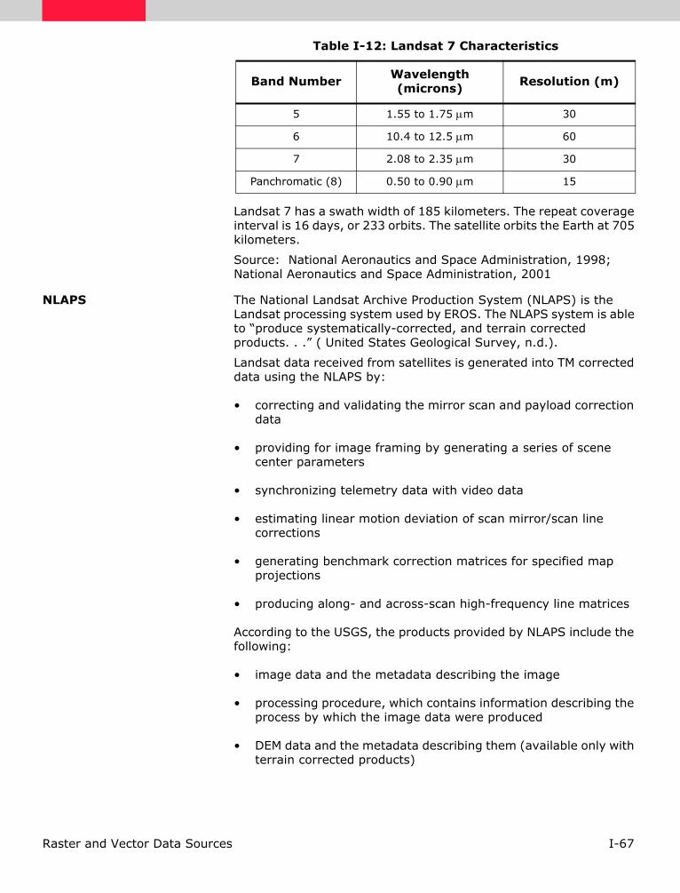
I-67Raster and Vector Data Sources

Landsat 7 has a swath width of 185 kilometers. The repeat coverage interval is 16 days, or 233 orbits. The satellite orbits the Earth at 705 kilometers.

Source: National Aeronautics and Space Administration, 1998; National Aeronautics and Space Administration, 2001

NLAPS The National Landsat Archive Production System (NLAPS) is the Landsat processing system used by EROS. The NLAPS system is able to “produce systematically-corrected, and terrain corrected products. . .” ( United States Geological Survey, n.d.).

Landsat data received from satellites is generated into TM corrected data using the NLAPS by:

• correcting and validating the mirror scan and payload correction data

• providing for image framing by generating a series of scene center parameters

• synchronizing telemetry data with video data

• estimating linear motion deviation of scan mirror/scan line corrections

• generating benchmark correction matrices for specified map projections

• producing along- and across-scan high-frequency line matrices

According to the USGS, the products provided by NLAPS include the following:

• image data and the metadata describing the image

• processing procedure, which contains information describing the process by which the image data were produced

• DEM data and the metadata describing them (available only with terrain corrected products)

5 1.55 to 1.75 µm 30

6 10.4 to 12.5 µm 60

7 2.08 to 2.35 µm 30

Panchromatic (8) 0.50 to 0.90 µm 15

Table I-12: Landsat 7 Characteristics

Band Number Wavelength (microns) Resolution (m)

I-68 Raster and Vector Data Sources

For information about the Landsat data processed by NLAPS, see "Landsat 1-5" on page I-62 and "Landsat 7" on page I-66.

Source: United States Geological Survey, n.d.

NOAA Polar Orbiter Data NOAA has sponsored several polar orbiting satellites to collect data of the Earth. These satellites were originally designed for meteorological applications, but the data gathered have been used in many fields—from agronomy to oceanography ( Needham, 1986).

The first of these satellites to be launched was the TIROS-N in 1978. Since the TIROS-N, five additional NOAA satellites have been launched. Of these, the last three are still in orbit gathering data.

AVHRR

The NOAA AVHRR data are small-scale data and often cover an entire country. The swath width is 2700 km and the satellites orbit at a height of approximately 833 km ( Kidwell, 1988; Needham, 1986).

The AVHRR system allows for direct transmission in real-time of data called High Resolution Picture Transmission (HRPT). It also allows for about ten minutes of data to be recorded over any portion of the world on two recorders on board the satellite. These recorded data are called Local Area Coverage (LAC). LAC and HRPT have identical formats; the only difference is that HRPT are transmitted directly and LAC are recorded.

There are three basic formats for AVHRR data which can be imported into ERDAS IMAGINE:

• LAC—data recorded on board the sensor with a spatial resolution of approximately 1.1 × 1.1 km,

• HRPT—direct transmission of AVHRR data in real-time with the same resolution as LAC, and

• GAC—data produced from LAC data by using only 1 out of every 3 scan lines. GAC data have a spatial resolution of approximately 4 × 4 km.

AVHRR data are available in 10-bit packed and 16-bit unpacked format. The term packed refers to the way in which the data are written to the tape. Packed data are compressed to fit more data on each tape ( Kidwell, 1988).

AVHRR images are useful for snow cover mapping, flood monitoring, vegetation mapping, regional soil moisture analysis, wildfire fuel mapping, fire detection, dust and sandstorm monitoring, and various geologic applications ( Lillesand and Kiefer, 1987). The entire globe can be viewed in 14.5 days. There may be four or five bands, depending on when the data were acquired.

I-69Raster and Vector Data Sources

AVHRR data have a radiometric resolution of 10-bits, meaning that each pixel has a possible data file value between 0 and 1023. AVHRR scenes may contain one band, a combination of bands, or all bands. All bands are referred to as a full set, and selected bands are referred to as an extract.

See “Ordering Raster Data” on page I-104 for information on the types of NOAA data available.

Use the Import/Export function to import AVHRR data.

OrbView-3 OrbView is a high-resolution satellite scheduled for launch by ORBIMAGE in the year 2000.

Table I-13: AVHRR Bands and Wavelengths

BandWavelengt

h (microns)

Comments

1, Vis-ible

0.58 to 0.68 µm

This band corresponds to the green reflectance of healthy vegetation and is important for vegetation discrimination.

2, NIR 0.725 to 1.10 µm

This band is especially responsive to the amount of vegetation biomass present in a scene. It is useful for crop identification and emphasizes soil/crop and land/water contrasts.

3, TIR 3.55 to 3.93 µm

This is a thermal band that can be used for snow and ice discrimination. It is also useful for detecting fires.

4, TIR 10.50 to 11.50 µm

(NOAA 6, 8, 10)

10.30 to 11.30 µm

(NOAA 7, 9, 11)

This band is useful for vegetation and crop stress detection. It can also be used to locate geothermal activity.

5, TIR 10.50 to 11.50 µm

(NOAA 6, 8, 10)

11.50 to 12.50 µm

(NOAA 7, 9, 11)

See Band 4, above.

I-70 Raster and Vector Data Sources

The OrbView-3 satellite will provide both 1 m panchromatic imagery and 4 m multispectral imagery. “One-meter imagery will enable the viewing of houses, automobiles and aircraft, and will make it possible to create highly precise digital maps and three-dimensional fly-through scenes. Four-meter multispectral imagery will provide color and infrared information to further characterize cities, rural areas and undeveloped land from space” ( ORBIMAGE, 1999). Specific applications include telecommunications and utilities, agriculture and forestry.

OrbView-3’s swath width is 8 km, with an image area of 64 km2. The revisit time is less than 3 days. OrbView-3 orbits the Earth at an altitude of 470 km.

Source: ORBIMAGE, 1999; ORBIMAGE, 2000

SeaWiFS The Sea-viewing Wide Field-of-View Sensor (SeaWiFS) instrument is on-board the SeaStar spacecraft, which was launched in 1997. The SeaStar spacecraft’s orbit is circular, at an altitude of 705 km.The satellite uses an attitude control system (ACS), which maintains orbit, as well as performs solar and lunar calibration maneuvers. The ACS also provides attitude information within one SeaWiFS pixel.

The SeaWiFS instrument is made up of an optical scanner and an electronics module. The swath width is 2,801 km LAC/HRPT (958.3 degrees) and 1,502 km GAC (45 degrees). The spatial resolution is 1.1 km LAC and 4.5 km GAC. The revisit time is one day.

Table I-14: OrbView-3 Bands and Spectral Ranges

Bands Spectral Range

1 450 to 520 nm

2 520 to 600 nm

3 625 to 695 nm

4 760 to 900 nm

Panchromatic 450 to 900 nm

Table I-15: SeaWiFS Bands and Wavelengths

Band Wavelength (nanometers)

1, Blue 402 to 422 nm

2, Blue 433 to 453 nm

3, Cyan 480 to 500 nm

4, Green 500 to 520 nm

5, Green 545 to 565 nm

I-71Raster and Vector Data Sources

Source: National Aeronautics and Space Administration, 1999; Center for Health Applications of Aerospace Related Technologies, 1998

SPOT The first SPOT satellite, developed by the French Centre National d’Etudes Spatiales (CNES), was launched in early 1986. The second SPOT satellite was launched in 1990 and the third was launched in 1993. The sensors operate in two modes, multispectral and panchromatic. SPOT is commonly referred to as a pushbroom scanner meaning that all scanning parts are fixed, and scanning is accomplished by the forward motion of the scanner. SPOT pushes 3000/6000 sensors along its orbit. This is different from Landsat which scans with 16 detectors perpendicular to its orbit.

The SPOT satellite can observe the same area on the globe once every 26 days. The SPOT scanner normally produces nadir views, but it does have off-nadir viewing capability. Off-nadir refers to any point that is not directly beneath the detectors, but off to an angle. Using this off-nadir capability, one area on the Earth can be viewed as often as every 3 days.

This off-nadir viewing can be programmed from the ground control station, and is quite useful for collecting data in a region not directly in the path of the scanner or in the event of a natural or man-made disaster, where timeliness of data acquisition is crucial. It is also very useful in collecting stereo data from which elevation data can be extracted.

The width of the swath observed varies between 60 km for nadir viewing and 80 km for off-nadir viewing at a height of 832 km ( Jensen, 1996).

Panchromatic

SPOT Panchromatic (meaning sensitive to all visible colors) has 10 × 10 m spatial resolution, contains 1 band—0.51 to 0.73 µm—and is similar to a black and white photograph. It has a radiometric resolution of 8 bits ( Jensen, 1996).

XS

SPOT XS, or multispectral, has 20 × 20 m spatial resolution, 8-bit radiometric resolution, and contains 3 bands ( Jensen, 1996).

6, Red 660 to 680 nm

7, NIR 745 to 785 nm

8, NIR 845 to 885 nm

Table I-15: SeaWiFS Bands and Wavelengths

Band Wavelength (nanometers)

I-72 Raster and Vector Data Sources

Figure I-25: SPOT Panchromatic vs. SPOT XS

See “Ordering Raster Data” for information on the types of SPOT data available.

Table I-16: SPOT XS Bands and Wavelengths

BandWavelengt

h (microns)

Comments

1, Green 0.50 to 0.59 µm

This band corresponds to the green reflectance of healthy vegetation.

2, Red 0.61 to 0.68 µm

This band is useful for discriminating between plant species. It is also useful for soil boundary and geological boundary delineations.

3, Reflec-tive IR

0.79 to 0.89 µm

This band is especially responsive to the amount of vegetation biomass present in a scene. It is useful for crop identification and emphasizes soil/crop and land/water contrasts.

SPOT Panchromatic vs XS

1 band

3 bands

1 pixel=20x20m

1 pixel=10x10m

Panchromatic

XS

radiometricresolution

0-255

I-73Raster and Vector Data Sources

Stereoscopic Pairs

Two observations can be made by the panchromatic scanner on successive days, so that the two images are acquired at angles on either side of the vertical, resulting in stereoscopic imagery. Stereoscopic imagery can also be achieved by using one vertical scene and one off-nadir scene. This type of imagery can be used to produce a single image, or topographic and planimetric maps ( Jensen, 1996).

Topographic maps indicate elevation. Planimetric maps correctly represent horizontal distances between objects ( Star and Estes, 1990).

See “Topographic Data” on page I-98 and "Terrain Analysis" for more information about topographic data and how SPOT stereopairs and aerial photographs can be used to create elevation data and orthographic images.

SPOT4 The SPOT4 satellite was launched in 1998. SPOT4 carries High Resolution Visible Infrared (HR VIR) instruments that obtain information in the visible and near-infrared spectral bands.

The SPOT4 satellite orbits the Earth at 822 km at the Equator. The SPOT4 satellite has two sensors on board: a multispectral sensor, and a panchromatic sensor. The multispectral scanner has a pixel size of 20 × 20 m, and a swath width of 60 km. The panchromatic scanner has a pixel size of 10 × 10 m, and a swath width of 60 km.

Source: SPOT Image, 1998; SPOT Image, 1999; Center for Health Applications of Aerospace Related Technologies, 2000c.

Radar Data Simply put, radar data are produced when:

• a radar transmitter emits a beam of micro or millimeter waves,

• the waves reflect from the surfaces they strike, and

Table I-17: SPOT4 Bands and Wavelengths

Band Wavelength

1, Green 0.50 to 0.59 µm

2, Red 0.61 to 0.68 µm

3, (near-IR) 0.78 to 0.89 µm

4, (mid-IR) 1.58 to 1.75 µm

Panchromatic 0.61 to 0.68 µm

I-74 Raster and Vector Data Sources

• the backscattered radiation is detected by the radar system’s receiving antenna, which is tuned to the frequency of the transmitted waves.

The resultant radar data can be used to produce radar images.

While there is a specific importer for data from RADARSAT and others, most types of radar image data can be imported into ERDAS IMAGINE with the Generic import option of Import/Export. The Generic SAR Node of the IMAGINE Radar Mapping Suite™ can be used to create or edit the radar ephemeris.

A radar system can be airborne, spaceborne, or ground-based. Airborne radar systems have typically been mounted on civilian and military aircraft, but in 1978, the radar satellite Seasat-1 was launched. The radar data from that mission and subsequent spaceborne radar systems have been a valuable addition to the data available for use in GIS processing. Researchers are finding that a combination of the characteristics of radar data and visible/infrared data is providing a more complete picture of the Earth. In the last decade, the importance and applications of radar have grown rapidly.

Advantages of Using Radar Data

Radar data have several advantages over other types of remotely sensed imagery:

• Radar microwaves can penetrate the atmosphere day or night under virtually all weather conditions, providing data even in the presence of haze, light rain, snow, clouds, or smoke.

• Under certain circumstances, radar can partially penetrate arid and hyperarid surfaces, revealing subsurface features of the Earth.

• Although radar does not penetrate standing water, it can reflect the surface action of oceans, lakes, and other bodies of water. Surface eddies, swells, and waves are greatly affected by the bottom features of the water body, and a careful study of surface action can provide accurate details about the bottom features.

Radar Sensors Radar images are generated by two different types of sensors:

• SLAR (Side-looking Airborne Radar)—uses an antenna which is fixed below an aircraft and pointed to the side to transmit and receive the radar signal. (See Figure I-26.)

• SAR—uses a side-looking, fixed antenna to create a synthetic aperture. SAR sensors are mounted on satellites and the NASA Space Shuttle. The sensor transmits and receives as it is moving. The signals received over a time interval are combined to create the image.

I-75Raster and Vector Data Sources

Both SLAR and SAR systems use side-looking geometry. Figure I-26 shows a representation of an airborne SLAR system.

Figure I-26: SLAR Radar

Source: Lillesand and Kiefer, 1987

Figure I-27 shows a graph of the data received from the radiation transmitted in Figure I-26. Notice how the data correspond to the terrain in Figure I-26. These data can be used to produce a radar image of the target area. A target is any object or feature that is the subject of the radar scan.

Figure I-27: Received Radar Signal

Active and Passive Sensors

An active radar sensor gives off a burst of coherent radiation that reflects from the target, unlike a passive microwave sensor which simply receives the low-level radiation naturally emitted by targets.

RangeDirection

AzimuthDirection

Sensor Heightat Nadir

AzimuthResolutionPrevious

ImageLines

BeamWidth

Tre

es

Val

ley

Hill

Hill

Shad

owTre

es

Time

Str

ength

(D

N)

I-76 Raster and Vector Data Sources

Like the coherent light from a laser, the waves emitted by active sensors travel in phase and interact minimally on their way to the target area. After interaction with the target area, these waves are no longer in phase. This is due to the different distances they travel from different targets, or single versus multiple bounce scattering.

Figure I-28: Radar Reflection from Different Sources and Distances

Source: Lillesand and Kiefer, 1987

Currently, these bands are commonly used for radar imaging systems:

More information about these radar systems is given later in this chapter.

Diffuse reflector Specularreflector

Cornerreflector

Radar waves are transmitted in

Once reflected, they are out of phase, interfering with each other and producing speckle noise.

Table I-18: Commonly Used Bands for Radar Imaging

Band

Frequency Range

Wavelength Range Radar System

X 5.20-10.90 GHz

5.77-2.75 cm

USGS SLAR

C 3.9-6.2 GHz 3.8-7.6 cm ERS-1, RADARSAT

L 0.39-1.55 GHz 76.9-19.3 cm

SIR-A,B, Almaz, FUYO-1 (JERS-1)

P 0.225-0.391 GHz

40.0-76.9 cm

AIRSAR

I-77Raster and Vector Data Sources

Radar bands were named arbitrarily when radar was first developed by the military. The letter designations have no special meaning.

NOTE: The C band overlaps the X band. Wavelength ranges may vary slightly between sensors.

Speckle Noise Once out of phase, the radar waves can interfere constructively or destructively to produce light and dark pixels known as speckle noise. Speckle noise in radar data must be reduced before the data can be utilized. However, the radar image processing programs used to reduce speckle noise also produce changes to the image. This consideration, combined with the fact that different applications and sensor outputs necessitate different speckle removal models, has lead ERDAS to offer several speckle reduction algorithms.

When processing radar data, the order in which the image processing programs are implemented is crucial. This is especially true when considering the removal of speckle noise. Since any image processing done before removal of the speckle results in the noise being incorporated into and degrading the image, do not rectify, correct to ground range, or in any way resample the pixel values before removing speckle noise. A rotation using nearest neighbor might be permissible.

The IMAGINE Radar Interpreter™ allows you to:

• import radar data into the GIS as a stand-alone source or as an additional layer with other imagery sources

• remove speckle noise

• enhance edges

• perform texture analysis

• perform radiometric and slant-to-ground range correction

IMAGINE OrthoRadar™ allows you to orthorectify radar imagery.

The IMAGINE InSAR™ module allows you to generate DEMs from SAR data using interferometric techniques.

The IMAGINE StereoSAR DEM™ module allows you to generate DEMs from SAR data using stereoscopic techniques.

See "Enhancement" and "Radar Concepts" for more information on radar imagery enhancement.

Applications for Radar Data

Radar data can be used independently in GIS applications or combined with other satellite data, such as Landsat, SPOT, or AVHRR. Possible GIS applications for radar data include:

I-78 Raster and Vector Data Sources

• Geology—radar’s ability to partially penetrate land cover and sensitivity to micro relief makes radar data useful in geologic mapping, mineral exploration, and archaeology.

• Classification—a radar scene can be merged with visible/infrared data as an additional layer(s) in vegetation classification for timber mapping, crop monitoring, etc.

• Glaciology—the ability to provide imagery of ocean and ice phenomena makes radar an important tool for monitoring climatic change through polar ice variation.

• Oceanography—radar is used for wind and wave measurement, sea-state and weather forecasting, and monitoring ocean circulation, tides, and polar oceans.

• Hydrology—radar data are proving useful for measuring soil moisture content and mapping snow distribution and water content.

• Ship monitoring—the ability to provide day/night all-weather imaging, as well as detect ships and associated wakes, makes radar a tool that can be used for ship navigation through frozen ocean areas such as the Arctic or North Atlantic Passage.

• Offshore oil activities—radar data are used to provide ice updates for offshore drilling rigs, determining weather and sea conditions for drilling and installation operations, and detecting oil spills.

• Pollution monitoring—radar can detect oil on the surface of water and can be used to track the spread of an oil spill.

Current Radar Sensors Table I-19, “Current Radar Sensors” gives a brief description of currently available radar sensors. This is not a complete list of such sensors, but it does represent the ones most useful for GIS applications.

Table I-19: Current Radar Sensors

ERS-1, 2 JERS-1 SIR-A, B SIR-C RADARSAT Almaz-1

Availability opera-tional

defunct 1981, 1984

1994 operational 1991-1992

Resolution 12.5 m 18 m 25 m 25 m 10-100 m 15 m

Revisit Time 35 days 44 days NA NA 3 days NA

Scene Area 100 × 100 km

75 × 100 km

30 ×60 km

variable swath

50 ×50 to 500 ×500

km

40 ×100 km

I-79Raster and Vector Data Sources

Almaz-1

Almaz was launched by the Soviet Union in 1987. The SAR operated with a single frequency SAR, which was attached to a spacecraft. Almaz-1 provided optically-processed data. The Almaz mission was largely kept secret

Almaz-1 was launched in 1991, and provides S-band information. It also includes a “single polarization SAR as well as a sounding radiometric scanner (RMS) system and several infrared bands” ( Atlantis Scientific, Inc., 1997).

The swath width of Almaz-1 is 20-45 km, the range resolution is 15-30 m, and the azimuth resolution is 15 m.

Source: National Aeronautics and Space Administration, 1996; Atlantis Scientific, Inc., 1997

ERS-1

ERS-1, a radar satellite, was launched by ESA in July of 1991. One of its primary instruments is the Along-Track Scanning Radiometer (ATSR). The ATSR monitors changes in vegetation of the Earth’s surface.

The instruments aboard ERS-1 include: SAR Image Mode, SAR Wave Mode, Wind Scatterometer, Radar Altimeter, and Along Track Scanning Radiometer-1 ( European Space Agency, 1997).

ERS-1 receiving stations are located all over the world, in countries such as Sweden, Norway, and Canada.

Some of the information that is obtained from the ERS-1 (as well as ERS-2, to follow) includes:

• maps of the surface of the Earth through clouds

• physical ocean features and atmospheric phenomena

• maps and ice patterns of polar regions

• database information for use in modeling

• surface elevation changes

Bands C band L band L band L, C, X bands

C band C band

Table I-19: Current Radar Sensors

I-80 Raster and Vector Data Sources

According to ESA,

. . .ERS-1 provides both global and regional views of the Earth, regardless of cloud coverage and sunlight conditions. An operational near-real-time capability for data acquisition, processing and dissemination, offering global data sets within three hours of observation, has allowed the development of time-critical applications particularly in weather, marine and ice forecasting, which are of great importance for many industrial activities ( European Space Agency, 1995).

Source: European Space Agency, 1995

ERS-2

ERS-2, a radar satellite, was launched by ESA in April of 1995. It has an instrument called GOME, which stands for Global Ozone Monitoring Experiment. This instrument is designed to evaluate atmospheric chemistry. ERS-2, like ERS-1 makes use of the ATSR.

The instruments aboard ERS-2 include: SAR Image Mode, SAR Wave Mode, Wind Scatterometer, Radar Altimeter, Along Track Scanning Radiometer-2, and the Global Ozone Monitoring Experiment.

ERS-2 receiving stations are located all over the world. Facilities that process and archive ERS-2 data are also located around the globe.

One of the benefits of the ERS-2 satellite is that, along with ERS-1, it can provide data from the exact same type of synthetic aperture radar (SAR).

ERS-2 provides many different types of information. See “ERS-1” on page I-79 for some of the most common types. Data obtained from ERS-2 used in conjunction with that from ERS-1 enables you to perform interferometric tasks. Using the data from the two sensors, DEMs can be created.

For information about ERDAS IMAGINE’s interferometric software, IMAGINE InSAR, see “IMAGINE InSAR Theory” on page II-216.

Source: European Space Agency, 1995

JERS-1

JERS stands for Japanese Earth Resources Satellite. The JERS-1 satellite was launched in February of 1992, with an SAR instrument and a 4-band optical sensor aboard. The SAR sensor’s ground resolution is 18 m, and the optical sensor’s ground resolution is roughly 18 m across-track and 24 m along-track. The revisit time of the satellite is every 44 days. The satellite travels at an altitude of 568 km, at an inclination of 97.67°.

I-81Raster and Vector Data Sources

1 Viewing 15.3° forward

Source: Earth Remote Sensing Data Analysis Center, 2000.

JERS-1 data comes in two different formats: European and Worldwide. The European data format consists mainly of coverage for Europe and Antarctica. The Worldwide data format has images that were acquired from stations around the globe. According to NASA, “a reduction in transmitter power has limited the use of JERS-1 data” ( National Aeronautics and Space Administration, 1996).

Source: Eurimage, 1998; National Aeronautics and Space Administration, 1996.

RADARSAT

RADARSAT satellites carry SARs, which are capable of transmitting signals that can be received through clouds and during nighttime hours. RADARSAT satellites have multiple imaging modes for collecting data, which include Fine, Standard, Wide, ScanSAR Narrow, ScanSAR Wide, Extended (H), and Extended (L). The resolution and swath width varies with each one of these modes, but in general, Fine offers the best resolution: 8 m.

Table I-20: JERS-1 Bands and Wavelengths

Band Wavelength

1 0.52 to 0.60 µm

2 0.63 to 0.69 µm

3 0.76 to 0.86 µm

41 0.76 to 0.86 µm

5 1.60 to 1.71 µm

6 2.01 to 2.12 µm

7 2.13 to 2.25 µm

8 2.27 to 2.40 µm

Table I-21: RADARSAT Beam Mode Resolution

Beam Mode Resolution

Fine Beam Mode 8 m

Standard Beam Mode 25 m

Wide Beam Mode 30 m

ScanSAR Narrow Beam Mode 50 m

ScanSAR Wide Beam Mode 100 m

I-82 Raster and Vector Data Sources

The types of RADARSAT image products include: Single Data, Single Look Complex, Path Image, Path Image Plus, Map Image, Precision Map Image, and Orthorectified. You can obtain this data in forms ranging from CD-ROM to print.

The RADARSAT satellite uses a single frequency, C-band. The altitude of the satellite is 496 miles, or 798 km. The satellite is able to image the entire Earth, and its path is repeated every 24 days. The swath width is 500 km. Daily coverage is available of the Arctic, and any area of Canada can be obtained within three days.

Source: RADARSAT, 1999; Space Imaging, 1999c

SIR-A

SIR stands for Spaceborne Imaging Radar. SIR-A was launched and began collecting data in 1981. The SIR-A mission built on the Seasat SAR mission that preceded it by increasing the incidence angle with which it captured images. The primary goal of the SIR-A mission was to collect geological information. This information did not have as pronounced a layover effect as previous imagery.

An important achievement of SIR-A data is that it is capable of penetrating surfaces to obtain information. For example, NASA says that the L-band capability of SIR-A enabled the discovery of dry river beds in the Sahara Desert.

SIR-1 uses L-band, has a swath width of 50 km, a range resolution of 40 m, and an azimuth resolution of 40 m ( Atlantis Scientific, Inc., 1997).

For information on the ERDAS IMAGINE software that reduces layover effect, IMAIGNE OrthoRadar, see “IMAGINE OrthoRadar Theory” on page II-197.

Source: National Aeronautics and Space Administration, 1995a; National Aeronautics and Space Administration, 1996; Atlantis Scientific, Inc., 1997.

SIR-B

SIR-B was launched and began collecting data in 1984. SIR-B improved over SIR-A by using an articulating antenna. This antenna allowed the incidence angle to range between 15 and 60 degrees. This enabled the mapping of surface features using “multiple-incidence angle backscatter signatures” ( National Aeronautics and Space Administration, 1996).

Extended High Beam Mode 25 m

Low Beam Mode 35 m

Table I-21: RADARSAT Beam Mode Resolution

Beam Mode Resolution

I-83Raster and Vector Data Sources

SIR-B uses L-band, has a swath width of 10-60 km, a range resolution of 60-10 m, and an azimuth resolution of 25 m ( Atlantis Scientific, Inc., 1997).

Source: National Aeronautics and Space Administration, 1995a, National Aeronautics and Space Administration, 1996; Atlantis Scientific, Inc., 1997.

SIR-C

SIR-C is part of a radar system, SIR-C/X-SAR, which was launched in 1994. The system is able to “. . .measure, from space, the radar signature of the surface at three different wavelengths, and to make measurements for different polarizations at two of those wavelengths” ( National Aeronautics and Space Administration, 1997). Moreover, it can supply “. . .images of the magnitude of radar backscatter for four polarization combinations” ( National Aeronautics and Space Administration, 1995a).

The data provided by SIR-C/X-SAR allows measurement of the following:

• vegetation type, extent, and deforestation

• soil moisture content

• ocean dynamics, wave and surface wind speeds and directions

• volcanism and tectonic activity

• soil erosion and desertification

The antenna of the system is composed of three antennas: one at L-band, one at C-band, and one at X-band. The antenna was assembled by the Jet Propulsion Laboratory. The acquisition of data at three different wavelengths makes SIR-C/X-SAR data very useful. The SIR-C and X-SAR do not have to be operated together: they can also be operated independent of one another.

SIR-C/X-SAR data come in resolutions from 10 to 200 m. The swath width of the sensor varies from 15 to 90 km, which depends on the direction the antenna is pointing. The system orbits the Earth at 225 km above the surface.

Source: National Aeronautics and Space Administration, 1995a, National Aeronautics and Space Administration, 1997.

Table I-22: SIR-C/X-SAR Bands and Frequencies

Bands Wavelength

L-Band 0.235 m

C-Band 0.058 m

X-Band 0.031 m

I-84 Raster and Vector Data Sources

Future Radar Sensors Several radar satellites are planned for launch within the next several years, but only a few programs will be successful. Following are two scheduled programs which are known to be highly achievable.

Light SAR

NASA and Jet Propulsion Laboratories (JPL) are currently designing a radar satellite called Light SAR. Present plans are for this to be a multipolar sensor operating at L-band.

Radarsat-2

The Canadian Space Agency is working on the follow-on system to Radarsat 1. Present plans are to include multipolar, C-band imagery.

Image Data from Aircraft

Image data can also be acquired from multispectral scanners or radar sensors aboard aircraft, as well as satellites. This is useful if there is not time to wait for the next satellite to pass over a particular area, or if it is necessary to achieve a specific spatial or spectral resolution that cannot be attained with satellite sensors.

For example, this type of data can be beneficial in the event of a natural or man-made disaster, because there is more control over when and where the data are gathered.

Two common types of airborne image data are:

• Airborne Synthetic Aperture Radar (AIRSAR)

• Airborne Visible/Infrared Imaging Spectrometer (AVIRIS)

AIRSAR AIRSAR is an experimental airborne radar sensor developed by JPL, Pasadena, California, under a contract with NASA. AIRSAR data have been available since 1983.

This sensor collects data at three frequencies:

• C-band

• L-band

• P-band

Because this sensor measures at three different wavelengths, different scales of surface roughness are obtained. The AIRSAR sensor has an IFOV of 10 m and a swath width of 12 km.

AIRSAR data have been used in many applications such as measuring snow wetness, classifying vegetation, and estimating soil moisture.

NOTE: These data are distributed in a compressed format. They must be decompressed before loading with an algorithm available from JPL. See “Addresses to Contact” for contact information.

I-85Raster and Vector Data Sources

AVIRIS The AVIRIS was also developed by JPL under a contract with NASA. AVIRIS data have been available since 1987.

This sensor produces multispectral data that have 224 narrow bands. These bands are 10 nm wide and cover the spectral range of .4 - 2.4 nm. The swath width is 11 km, and the spatial resolution is 20 m. This sensor is flown at an altitude of approximately 20 km. The data are recorded at 10-bit radiometric resolution.

Daedalus TMS Daedalus is a thematic mapper simulator (TMS), which simulates the characteristics, such as spatial and radiometric, of the TM sensor on Landsat spacecraft.

The Daedalus TMS orbits at 65,000 feet, and has a ground resolution of 25 meters. The total scan angle is 43 degrees, and the swath width is 15.6 km. Daedalus TMS is flown aboard the NASA ER-2 aircraft.

The Daedalus TMS spectral bands are as follows:

Source: National Aeronautics and Space Administration, 1995b

Image Data from Scanning

Hardcopy maps and photographs can be incorporated into the ERDAS IMAGINE environment through the use of a scanning device to transfer them into a digital (raster) format.

Table I-23: Daedalus TMS Bands and Wavelengths

Daedalus Channel TM Band Wavelength

1 A 0.42 to 0.45 µm

2 1 0.45 to 0.52 µm

3 2 0.52 to 0.60 µm

4 B 0.60 to 0.62 µm

5 3 0.63 to 0.69 µm

6 C 0.69 to 0.75 µm

7 4 0.76 to 0.90 µm

8 D 0.91 to 1.05 µm

9 5 1.55 to 1.75 µm

10 7 2.08 to 2.35 µm

11 6 8.5 to 14.0 µm low gain

12 6 8.5 to 14.0 µm high gain

I-86 Raster and Vector Data Sources

In scanning, the map, photograph, transparency, or other object to be scanned is typically placed on a flat surface, and the scanner scans across the object to record the image. The image is then transferred from analog to digital data.

There are many commonly used scanners for GIS and other desktop applications, such as Eikonix (Eikonix Corp., Huntsville, Alabama) or Vexcel (Vexcel Imaging Corp., Boulder, Colorado). Many scanners produce a Tagged Image File Format (TIFF) file, which can be used directly by ERDAS IMAGINE.

Use the Import/Export function to import scanned data.Eikonix data can be obtained in the ERDAS IMAGINE .img format using the XSCAN™ Tool by Ektron and then imported directly into ERDAS IMAGINE.

Photogrammetric Scanners

There are photogrammetric high quality scanners and desktop scanners. Photogrammetric quality scanners are special devices capable of high image quality and excellent positional accuracy. Use of this type of scanner results in geometric accuracies similar to traditional analog and analytical photogrammetric instruments. These scanners are necessary for digital photogrammetric applications that have high accuracy requirements.

These units usually scan only film because film is superior to paper, both in terms of image detail and geometry. These units usually have a Root Mean Square Error (RMSE) positional accuracy of 4 microns or less, and are capable of scanning at a maximum resolution of 5 to 10 microns.

The required pixel resolution varies depending on the application. Aerial triangulation and feature collection applications often scan in the 10 to 15 micron range. Orthophoto applications often use 15- to 30-micron pixels. Color film is less sharp than panchromatic, therefore color ortho applications often use 20- to 40-micron pixels.

Desktop Scanners Desktop scanners are general purpose devices. They lack the image detail and geometric accuracy of photogrammetric quality units, but they are much less expensive. When using a desktop scanner, you should make sure that the active area is at least 9 × 9 inches (i.e., A3-type scanners), enabling you to capture the entire photo frame.

Desktop scanners are appropriate for less rigorous uses, such as digital photogrammetry in support of GIS or remote sensing applications. Calibrating these units improves geometric accuracy, but the results are still inferior to photogrammetric units. The image correlation techniques that are necessary for automatic tie point collection and elevation extraction are often sensitive to scan quality. Therefore, errors can be introduced into the photogrammetric solution that are attributable to scanning errors.

I-87Raster and Vector Data Sources

Aerial Photography Aerial photographs, such as NAPP photos, are most widely used data sources in photogrammetry. They can not be utilized in softcopy or digital photogrammetric applications until scanned. The standard dimensions of the aerial photos are 9 × 9 inches or 230 × 230 mm. The ground area covered by the photo depends on the scale. The scanning resolution determines the digital image file size and pixel size.

For example, for a 1:40,000 scale standard block of white aerial photos scanned at 25 microns (1016 dots per inch), the ground pixel size is 1 × 1 m2. The resulting file size is about 85 MB. It is not recommended to scan a photo with a scanning resolution less than 5 microns or larger than 5080 dpi.

DOQs DOQ stands for digital orthophoto quadrangle. USGS defines a DOQ as a computer-generated image of an aerial photo, which has been orthorectified to give it map coordinates. DOQs can provide accurate map measurements.

The format of the DOQ is a grayscale image that covers 3.75 minutes of latitude by 3.75 minutes of longitude. DOQs use the North American Datum of 1983, and the Universal Transverse Mercator projection. Each pixel of a DOQ represents a square meter. 3.75-minute quarter quadrangles have a 1:12,000 scale. 7.5-minute quadrangles have a 1:24,000 scale. Some DOQs are available in color-infrared, which is especially useful for vegetation monitoring.

DOQs can be used in land use and planning, management of natural resources, environmental impact assessments, and watershed analysis, among other applications. A DOQ can also be used as “a cartographic base on which to overlay any number of associated thematic layers for displaying, generating, and modifying planimetric data or associated data files” ( United States Geological Survey, 1999b).

According to the USGS:

DOQ production begins with an aerial photo and requires four elements: (1) at least three ground positions that can be identified within the photo; (2) camera calibration specifications, such as focal length; (3) a digital elevation model (DEM) of the area covered by the photo; (4) and a high-resolution digital image of the photo, produced by scanning. The photo is processed pixel by pixel to produce an image with features in true geographic positions ( United States Geological Survey, 1999b).

Source: United States Geological Survey, 1999b.

ADRG Data ADRG (ARC Digitized Raster Graphic) data come from the National Imagery and Mapping Agency (NIMA), which was formerly known as the Defense Mapping Agency (DMA). ADRG data are primarily used for military purposes by defense contractors. The data are in 128 × 128 pixel tiled, 8-bit format stored on CD-ROM. ADRG data provide large amounts of hardcopy graphic data without having to store and maintain the actual hardcopy graphics.

I-88 Raster and Vector Data Sources

ADRG data consist of digital copies of NIMA hardcopy graphics transformed into the ARC system and accompanied by ASCII encoded support files. These digital copies are produced by scanning each hardcopy graphic into three images: red, green, and blue. The data are scanned at a nominal collection interval of 100 microns (254 lines per inch). When these images are combined, they provide a 3-band digital representation of the original hardcopy graphic.

ARC System The ARC system (Equal Arc-Second Raster Chart/Map) provides a rectangular coordinate and projection system at any scale for the Earth’s ellipsoid, based on the World Geodetic System 1984 (WGS 84). The ARC System divides the surface of the ellipsoid into 18 latitudinal bands called zones. Zones 1 - 9 cover the Northern hemisphere and zones 10 - 18 cover the Southern hemisphere. Zone 9 is the North Polar region. Zone 18 is the South Polar region.

Distribution Rectangles

For distribution, ADRG are divided into geographic data sets called Distribution Rectangles (DRs). A DR may include data from one or more source charts or maps. The boundary of a DR is a geographic rectangle that typically coincides with chart and map neatlines.

Zone Distribution Rectangles

Each DR is divided into Zone Distribution Rectangles (ZDRs). There is one ZDR for each ARC System zone covering any part of the DR. The ZDR contains all the DR data that fall within that zone’s limits. ZDRs typically overlap by 1,024 rows of pixels, which allows for easier mosaicking. Each ZDR is stored on the CD-ROM as a single raster image file (.IMG). Included in each image file are all raster data for a DR from a single ARC System zone, and padding pixels needed to fulfill format requirements. The padding pixels are black and have a zero value.

The padding pixels are not imported by ERDAS IMAGINE, nor are they counted when figuring the pixel height and width of each image.

ADRG File Format Each CD-ROM contains up to eight different file types which make up the ADRG format. ERDAS IMAGINE imports three types of ADRG data files:

• .OVR (Overview)

• .IMG (Image)

• .Lxx (Legend or marginalia data)

NOTE: Compressed ADRG (CADRG) is a different format, which may be imported or read directly.

I-89Raster and Vector Data Sources

The ADRG .IMG and .OVR file formats are different from the ERDAS IMAGINE .img and .ovr file formats.

.OVR (overview) The overview file contains a 16:1 reduced resolution image of the whole DR. There is an overview file for each DR on a CD-ROM.

Importing ADRG Subsets

Since DRs can be rather large, it may be beneficial to import a subset of the DR data for the application. ERDAS IMAGINE enables you to define a subset of the data from the preview image (see Figure I-30).

You can import from only one ZDR at a time. If a subset covers multiple ZDRs, they must be imported separately and mosaicked with the Mosaic option.

Figure I-29: ADRG Overview File Displayed in a Viewer

The white rectangle in Figure I-30 represents the DR. The subset area in this illustration would have to be imported as three files: one for each zone in the DR.

Notice how the ZDRs overlap. Therefore, the .IMG files for Zones 2 and 4 would also be included in the subset area.

I-90 Raster and Vector Data Sources

Figure I-30: Subset Area with Overlapping ZDRs

.IMG (scanned image data)

The .IMG files are the data files containing the actual scanned hardcopy graphic(s). Each .IMG file contains one ZDR plus padding pixels. The Import function converts the .IMG data files on the CD-ROM to the ERDAS IMAGINE file format (.img). The image file can then be displayed in a Viewer.

.Lxx (legend data) Legend files contain a variety of diagrams and accompanying information. This is information that typically appears in the margin or legend of the source graphic.

This information can be imported into ERDAS IMAGINE and viewed. It can also be added to a map composition with the ERDAS IMAGINE Map Composer.

Each legend file contains information based on one of these diagram types:

• Index (IN)—shows the approximate geographical position of the graphic and its relationship to other graphics in the region.

• Elevation/Depth Tint (EL)—depicts the colors or tints using a multicolored graphic that represent different elevations or depth bands on the printed map or chart.

• Slope (SL)—represents the percent and degree of slope appearing in slope bands.

• Boundary (BN)—depicts the geopolitical boundaries included on the map or chart.

Zone 4

Zone 3

Zone 2

overlap area

overlap areaSubset

Area

I-91Raster and Vector Data Sources

• Accuracy (HA, VA, AC)—depicts the horizontal and vertical accuracies of selected map or chart areas. AC represents a combined horizontal and vertical accuracy diagram.

• Geographic Reference (GE)—depicts the positioning information as referenced to the World Geographic Reference System.

• Grid Reference (GR)—depicts specific information needed for positional determination with reference to a particular grid system.

• Glossary (GL)—gives brief lists of foreign geographical names appearing on the map or chart with their English-language equivalents.

• Landmark Feature Symbols (LS)—depict navigationally-prominent entities.

ARC System Charts

The ADRG data on each CD-ROM are based on one of these chart types from the ARC system:

Each ARC System chart type has certain legend files associated with the image(s) on the CD-ROM. The legend files associated with each chart type are checked in Table I-25, “Legend Files for the ARC System Chart Types”.

Table I-24: ARC System Chart Types

ARC System Chart Type Scale

GNC (Global Navigation Chart) 1:5,000,000

JNC-A (Jet Navigation Chart - Air) 1:3,000,000

JNC (Jet Navigation Chart) 1:2,000,000

ONC (Operational Navigation Chart) 1:1,000,000

TPC (Tactical Pilot Chart) 1:500,000

JOG-A (Joint Operations Graphic - Air) 1:250,000

JOG-G (Joint Operations Graphic - Ground) 1:250,000

JOG-C (Joint Operations Graphic - Combined) 1:250,000

JOG-R (Joint Operations Graphic - Radar) 1:250,000

ATC (Series 200 Air Target Chart) 1:200,000

TLM (Topographic Line Map) 1:50,000

I-92 Raster and Vector Data Sources

ADRG File Naming Convention

The ADRG file naming convention is based on a series of codes: ssccddzz

• ss = the chart series code (see the table of ARC System charts)

• cc = the country code

• dd = the DR number on the CD-ROM (01-99). DRs are numbered beginning with 01 for the northwesternmost DR and increasing sequentially west to east, then north to south.

• zz = the zone rectangle number (01-18)

For example, in the ADRG filename JNUR0101.IMG:

• JN = Jet Navigation. This ADRG file is taken from a Jet Navigation chart.

• UR = Europe. The data is coverage of a European continent.

• 01 = This is the first DR on the CD-ROM, providing coverage of the northwestern edge of the image area.

• 01 = This is the first zone rectangle of the DR.

• .IMG = This file contains the actual scanned image data for a ZDR.

Table I-25: Legend Files for the ARC System Chart Types

ARC System Chart IN EL SL BN VA HA AC GE GR GL LS

GNC • •

JNC / JNC-A • • • • •

ONC • • • • •

TPC • • • • • •

JOG-A • • • • • • • •

JOG-G / JOG-C • • • • • • •

JOG-R • • • • • •

ATC • • • • •

TLM • • • • • •

I-93Raster and Vector Data Sources

You may change this name when the file is imported into ERDAS IMAGINE. If you do not specify a file name, ERDAS IMAGINE uses the ADRG file name for the image.

Legend File Names

Legend file names include a code to designate the type of diagram information contained in the file (see the previous legend file description). For example, the file JNUR01IN.L01 means:

• JN = Jet Navigation. This ADRG file is taken from a Jet Navigation chart.

• UR = Europe. The data is coverage of a European continent.

• 01 = This is the first DR on the CD-ROM, providing coverage of the northwestern edge of the image area.

• IN = This indicates that this file is an index diagram from the original hardcopy graphic.

• .L01 = This legend file contains information for the source graphic 01. The source graphics in each DR are numbered beginning with 01 for the northwesternmost source graphic, increasing sequentially west to east, then north to south. Source directories and their files include this number code within their names.

For more detailed information on ADRG file naming conventions, see the National Imagery and Mapping Agency Product Specifications for ARC Digitized Raster Graphics (ADRG), published by the NIMA Aerospace Center.

ADRI Data ADRI (ARC Digital Raster Imagery), like ADRG data, are also from the NIMA and are currently available only to Department of Defense contractors. The data are in 128 × 128 tiled, 8-bit format, stored on 8 mm tape in band sequential format.

ADRI consists of SPOT panchromatic satellite imagery transformed into the ARC system and accompanied by ASCII encoded support files.

Like ADRG, ADRI data are stored in the ARC system in DRs. Each DR consists of all or part of one or more images mosaicked to meet the ARC bounding rectangle, which encloses a 1 degree by 1 degree geographic area. (See Figure I-31.) Source images are orthorectified to mean sea level using NIMA Level I Digital Terrain Elevation Data (DTED) or equivalent data (Air Force Intelligence Support Agency, 1991).

I-94 Raster and Vector Data Sources

See the previous section on ADRG data for more information on the ARC system. See “DTED” for more information.

Figure I-31: Seamless Nine Image DR

In ADRI data, each DR contains only one ZDR. Each ZDR is stored as a single raster image file, with no overlapping areas.

There are six different file types that make up the ADRI format: two types of data files, three types of header files, and a color test patch file. ERDAS IMAGINE imports two types of ADRI data files:

• .OVR (Overview)

• .IMG (Image)

The ADRI .IMG and .OVR file formats are different from the ERDAS IMAGINE .img and .ovr file formats.

.OVR (overview) The overview file (.OVR) contains a 16:1 reduced resolution image of the whole DR. There is an overview file for each DR on a tape. The .OVR images show the mosaicking from the source images and the dates when the source images were collected. (See Figure I-32.) This does not appear on the ZDR image.

Image 1Image 2

Image 4

Image 8

Image 5

Image 6

Image 9

7

3

I-95Raster and Vector Data Sources

Figure I-32: ADRI Overview File Displayed in a Viewer

.IMG (scanned image data)

The .IMG files contain the actual mosaicked images. Each .IMG file contains one ZDR plus any padding pixels needed to fit the ARC boundaries. Padding pixels are black and have a zero data value. The ERDAS IMAGINE Import function converts the .IMG data files to the ERDAS IMAGINE file format (.img). The image file can then be displayed in a Viewer. Padding pixels are not imported, nor are they counted in image height or width.

ADRI File Naming Convention

The ADRI file naming convention is based on a series of codes: ssccddzz

• ss = the image source code:

- SP (SPOT panchromatic)- SX (SPOT multispectral) (not currently available)- TM (Landsat Thematic Mapper) (not currently available)

• cc = the country code

• dd = the DR number on the tape (01-99). DRs are numbered beginning with 01 for the northwesternmost DR and increasing sequentially west to east, then north to south.

• zz = the zone rectangle number (01-18)

For example, in the ADRI filename SPUR0101.IMG:

• SP = SPOT 10 m panchromatic image

• UR = Europe. The data is coverage of a European continent.

• 01 = This is the first Distribution Rectangle on the CD-ROM, providing coverage of the northwestern edge of the image area

I-96 Raster and Vector Data Sources

• 01 = This is the first zone rectangle of the Distribution Rectangle.

• .IMG = This file contains the actual scanned image data for a ZDR.

You may change this name when the file is imported into ERDAS IMAGINE. If you do not specify a file name, ERDAS IMAGINE uses the ADRI file name for the image.

Raster Product Format

The Raster Product Format (RPF), from NIMA, is primarily used for military purposes by defense contractors. RPF data are organized in 1536 × 1536 frames, with an internal tile size of 256 × 256 pixels. RPF data are stored in an 8-bit format, with or without a pseudocolor lookup table, on CD-ROM.

RPF Data are projected to the ARC system, based on the World Geodetic System 1984 (WGS 84). The ARC System divides the surface of the ellipsoid into 18 latitudinal bands called zones. Zones 1-9 cover the Northern hemisphere and zones A-J cover the Southern hemisphere. Zone 9 is the North Polar region. Zone J is the South Polar region

Polar data is projected to the Azimuthal Equidistant projection. In nonpolar zones, data is in the Equirectangular projection, which is proportional to latitude and longitude. ERDAS IMAGINE includes the option to use either Equirectangular or Geographic coordinates for nonpolar RPF data. The aspect ratio of projected RPF data is nearly 1; frames appear to be square, and measurement is possible. Unprojected RPFs seldom have an aspect of ratio of 1, but may be easier to combine with other data in Geographic coordinates.

Two military products are currently based upon the general RPF specification:

• Controlled Image Base (CIB)

• Compressed ADRG (CADRG)

RPF employs Vector Quantization (VQ) to compress the frames. A vector is a 4 × 4 tile of 8-bit pixel values. VQ evaluates all of the vectors within the image, and reduces each vector into a single 12-bit lookup value. Since only 4096 unique vector values are possible, VQ is lossy, but the space savings are substantial. Most of the processing effort of VQ is incurred in the compression stage, permitting fast decompression by the users of the data in the field.

RPF data are stored on CD-ROM, with the following structure:

• The root of the CD-ROM contains an RPF directory. This RPF directory is often referred to as the root of the product.

I-97Raster and Vector Data Sources

• The RPF directory contains a table-of-contents file, named A.TOC, which describes the location of all of the frames in the product, and

• The RPF directory contains one or more subdirectories containing RPF frame files. RPF frame file names typically encode the map zone and location of the frame within the map series.

• Overview images may appear at various points in the directory tree. Overview images illustrate the location of a set of frames with respect to political and geographic boundaries. Overview images typically have an .OVx file extension, such as .OVR or .OV1.

All RPF frames, overview images, and table-of-contents files are physically formatted within an NITF message. Since an RPF image is broken up into several NITF messages, ERDAS IMAGINE treats RPF and NITF as distinct formats.

Loading RPF Data

RPF frames may be imported or read directly. The direct read feature, included in ERDAS IMAGINE, is generally preferable since multiple frames with the same resolution can be read as a single image. Import may still be desirable if you wish to examine the metadata provided by a specific frame. ERDAS IMAGINE supplies four image types related to RPF:

• RPF Product—combines the entire contents of an RPF CD, excluding overview images, as a single image, provided all frames are within the same ARC map zone and resolution.The RPF directory at the root of the CD-ROM is the image to be loaded.

• RPF Cell—combines all of the frames within a given subdirectory, provided they all have the same resolution and reside within the same ARC map zone. The directory containing frames is the image to be read as an RPF cell.

• RPF Frame—reads a single frame file.

• RPF Overview—reads a single overview frame file.

CIB CIB is grayscale imagery produced from rectified imagery and physically formatted as a compressed RPF. CIB offers a compression ratio of 8:1 over its predecessor, ADRI. CIB is often based upon SPOT panchromatic data or reformatted ADRI data, but can be produced from other sources of imagery.

CADRG CADRG data consist of digital copies of NIMA hardcopy graphics transformed into the ARC system. The data are scanned at a nominal collection interval of 150 microns. The resulting image is 8-bit pseudocolor, which is physically formatted as a compressed RPF.

I-98 Raster and Vector Data Sources

CADRG is a successor to ADRG, Compressed Aeronautical Chart (CAC), and Compressed Raster Graphics (CRG). CADRG offers a compression ratio of 55:1 over ADRG, due to the coarser collection interval, VQ compression, and the encoding as 8-bit pseudocolor, instead of 24-bit truecolor.

Topographic Data Satellite data can also be used to create elevation, or topographic data through the use of stereoscopic pairs, as discussed above under SPOT. Radar sensor data can also be a source of topographic information, as discussed in "Terrain Analysis" However, most available elevation data are created with stereo photography and topographic maps.

ERDAS IMAGINE software can load and use:

• USGS DEMs

• DTED

Arc/second Format

Most elevation data are in arc/second format. Arc/second refers to data in the Latitude/Longitude (Lat/Lon) coordinate system. The data are not rectangular, but follow the arc of the Earth’s latitudinal and longitudinal lines.

Each degree of latitude and longitude is made up of 60 minutes. Each minute is made up of 60 seconds. Arc/second data are often referred to by the number of seconds in each pixel. For example, 3 arc/second data have pixels which are 3 × 3 seconds in size. The actual area represented by each pixel is a function of its latitude. Figure I-33 illustrates a 1° × 1° area of the Earth.

A row of data file values from a DEM or DTED file is called a profile. The profiles of DEM and DTED run south to north, that is, the first pixel of the record is the southernmost pixel.

I-99Raster and Vector Data Sources

Figure I-33: Arc/second Format

In Figure I-33, there are 1201 pixels in the first row and 1201 pixels in the last row, but the area represented by each pixel increases in size from the top of the file to the bottom of the file. The extracted section in the example above has been exaggerated to illustrate this point.

Arc/second data used in conjunction with other image data, such as TM or SPOT, must be rectified or projected onto a planar coordinate system such as UTM.

DEM DEMs are digital elevation model data. DEM was originally a term reserved for elevation data provided by the USGS, but it is now used to describe any digital elevation data.

DEMs can be:

• purchased from USGS (for US areas only)

• created from stereopairs (derived from satellite data or aerial photographs)

See "Terrain Analysis" for more information on using DEMs. See “Ordering Raster Data” on page I-104 for information on ordering DEMs.

USGS DEMs

There are two types of DEMs that are most commonly available from USGS:

• 1:24,000 scale, also called 7.5-minute DEM, is usually referenced to the UTM coordinate system. It has a spatial resolution of 30 × 30 m.

Arc/Second Format

1201

1201

1201

Lati tude

Long

itude

I-100 Raster and Vector Data Sources

• 1:250,000 scale is available only in Arc/second format.

Both types have a 16-bit range of elevation values, meaning each pixel can have a possible elevation of -32,768 to 32,767.

DEM data are stored in ASCII format. The data file values in ASCII format are stored as ASCII characters rather than as zeros and ones like the data file values in binary data.

DEM data files from USGS are initially oriented so that North is on the right side of the image instead of at the top. ERDAS IMAGINE rotates the data 90° counterclockwise as part of the Import process so that coordinates read with any ERDAS IMAGINE program are correct.

DTED DTED data are produced by the National Imagery and Mapping Agency (NIMA) and are available only to US government agencies and their contractors. DTED data are distributed on 9-track tapes and on CD-ROM.

There are two types of DTED data available:

• DTED 1 — a 1° × 1° area of coverage

• DTED 2 — a 1° × 1° or less area of coverage

Both are in Arc/second format and are distributed in cells. A cell is a 1° × 1° area of coverage. Both have a 16-bit range of elevation values.

Like DEMs, DTED data files are also oriented so that North is on the right side of the image instead of at the top. ERDAS IMAGINE rotates the data 90° counterclockwise as part of the Import process so that coordinates read with any ERDAS IMAGINE program are correct.

Using Topographic Data Topographic data have many uses in a GIS. For example, topographic data can be used in conjunction with other data to:

• calculate the shortest and most navigable path over a mountain range

• assess the visibility from various lookout points or along roads

• simulate travel through a landscape

• determine rates of snow melt

• orthocorrect satellite or airborne images

• create aspect and slope layers

• provide ancillary data from image classification

See "Terrain Analysis" for more information about using topographic and elevation data.

I-101Raster and Vector Data Sources

GPS Data

Introduction Global Positioning System (GPS) data has been in existence since the launch of the first satellite in the US Navigation System with Time and Ranging (NAVSTAR) system on February 22, 1978, and the availability of a full constellation of satellites since 1994. Initially, the system was available to US military personnel only, but from 1993 onwards the system started to be used (in a degraded mode) by the general public. There is also a Russian GPS system called GLONASS with similar capabilities.

The US NAVSTAR GPS consists of a constellation of 24 satellites orbiting the Earth, broadcasting data that allows a GPS receiver to calculate its spatial position.

Satellite Position Positions are determined through the traditional ranging technique. The satellites orbit the Earth (at an altitude of 20,200 km) in such a manner that several are always visible at any location on the Earth's surface. A GPS receiver with line of site to a GPS satellite can determine how long the signal broadcast by the satellite has taken to reach its location, and therefore can determine the distance to the satellite. Thus, if the GPS receiver can see three or more satellites and determine the distance to each, the GPS receiver can calculate its own position based on the known positions of the satellites (i.e., the intersection of the spheres of distance from the satellite locations). Theoretically, only three satellites should be required to find the 3D position of the receiver, but various inaccuracies (largely based on the quality of the clock within the GPS receiver that is used to time the arrival of the signal) mean that at least four satellites are generally required to determine a three-dimensional (3D) x, y, z position.

The explanation above is an over-simplification of the technique used, but does show the concept behind the use of the GPS system for determining position. The accuracy of that position is affected by several factors, including the number of satellites that can be seen by a receiver, but especially for commercial users by Selective Availability. Each satellite actually sends two signals at different frequencies. One is for civilian use and one for military use. The signal used for commercial receivers has an error introduced to it called Selective Availability. Selective Availability introduces a positional inaccuracy of up to 100m to commercial GPS receivers. This is mainly intended to limit the use of highly accurate GPS positioning to hostile users, but the errors can be ameliorated through various techniques, such as keeping the GPS receiver stationary; thereby allowing it to average out the errors, or through more advanced techniques discussed in the following sections.

I-102 Raster and Vector Data Sources

Differential Correction Differential Correction (or Differential GPS - DGPS) can be used to remove the majority of the effects of Selective Availability. The technique works by using a second GPS unit (or base station) that is stationary at a precisely known position. As this GPS knows where it actually is, it can compare this location with the position it calculates from GPS satellites at any particular time and calculate an error vector for that time (i.e., the distance and direction that the GPS reading is in error from the real position). A log of such error vectors can then be compared with GPS readings taken from the first, mobile unit (the field unit that is actually taking GPS location readings of features). Under the assumption that the field unit had line of site to the same GPS satellites to acquire its position as the base station, each field-read position (with an appropriate time stamp) can be compared to the error vector for that time and the position corrected using the inverse of the vector. This is generally performed using specialist differential correction software.

Real Time Differential GPS (RDGPS) takes this technique one step further by having the base station communicate the error vector via radio to the field unit in real time. The field unit can then automatically updates its own location in real time. The main disadvantage of this technique is that the range that a GPS base station can broadcast over is generally limited, thereby restricting the range the mobile unit can be used away from the base station. One of the biggest uses of this technique is for ocean navigation in coastal areas, where base stations have been set up along coastlines and around ports so that the GPS systems on board ships can get accurate real time positional information to help in shallow-water navigation.

Applications of GPS Data GPS data finds many uses in remote sensing and GIS applications, such as:

• Collection of ground truth data, even spectral properties of real-world conditions at known geographic positions, for use in image classification and validation. The user in the field identifies a homogeneous area of identifiable land cover or use on the ground and records its location using the GPS receiver. These locations can then be plotted over an image to either train a supervised classifier or to test the validity of a classification.

• Moving map applications take the concept of relating the GPS positional information to your geographic data layers one step further by having the GPS position displayed in real time over the geographical data layers. Thus you take a computer out into the field and connect the GPS receiver to the computer, usually via the serial port. Remote sensing and GIS data layers are then displayed on the computer and the positional signal from the GPS receiver is plotted on top of them.

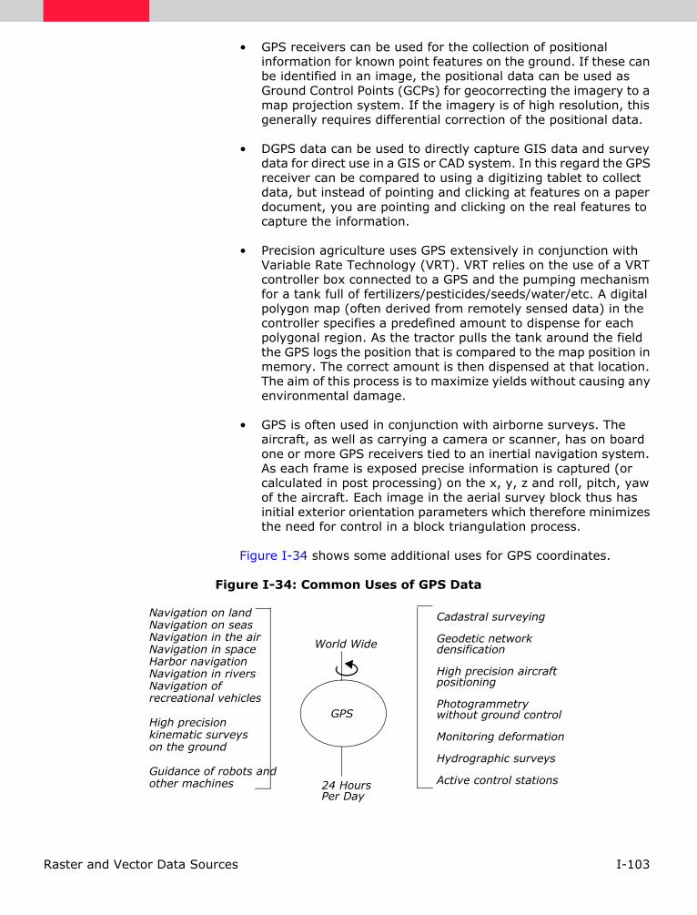
I-103Raster and Vector Data Sources

• GPS receivers can be used for the collection of positional information for known point features on the ground. If these can be identified in an image, the positional data can be used as Ground Control Points (GCPs) for geocorrecting the imagery to a map projection system. If the imagery is of high resolution, this generally requires differential correction of the positional data.

• DGPS data can be used to directly capture GIS data and survey data for direct use in a GIS or CAD system. In this regard the GPS receiver can be compared to using a digitizing tablet to collect data, but instead of pointing and clicking at features on a paper document, you are pointing and clicking on the real features to capture the information.

• Precision agriculture uses GPS extensively in conjunction with Variable Rate Technology (VRT). VRT relies on the use of a VRT controller box connected to a GPS and the pumping mechanism for a tank full of fertilizers/pesticides/seeds/water/etc. A digital polygon map (often derived from remotely sensed data) in the controller specifies a predefined amount to dispense for each polygonal region. As the tractor pulls the tank around the field the GPS logs the position that is compared to the map position in memory. The correct amount is then dispensed at that location. The aim of this process is to maximize yields without causing any environmental damage.

• GPS is often used in conjunction with airborne surveys. The aircraft, as well as carrying a camera or scanner, has on board one or more GPS receivers tied to an inertial navigation system. As each frame is exposed precise information is captured (or calculated in post processing) on the x, y, z and roll, pitch, yaw of the aircraft. Each image in the aerial survey block thus has initial exterior orientation parameters which therefore minimizes the need for control in a block triangulation process.

Figure I-34 shows some additional uses for GPS coordinates.

Figure I-34: Common Uses of GPS Data

Navigation on landNavigation on seasNavigation in the airNavigation in spaceHarbor navigationNavigation in riversNavigation of recreational vehicles

High precision kinematic surveys on the ground

Guidance of robots andother machines

Cadastral surveying

Geodetic networkdensification

High precision aircraftpositioning

Photogrammetry without ground control

Monitoring deformation

Hydrographic surveys

Active control stations

GPS

24 HoursPer Day

World Wide

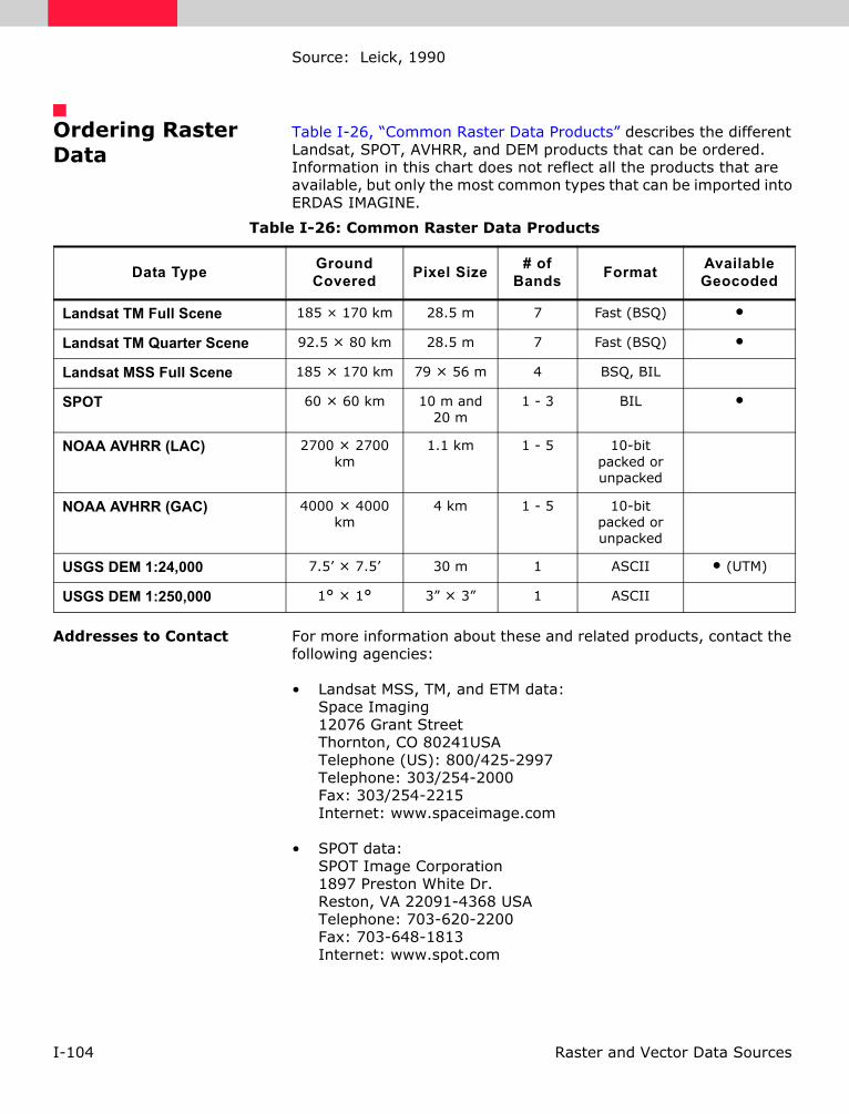
I-104 Raster and Vector Data Sources

Source: Leick, 1990

Ordering Raster Data

Table I-26, “Common Raster Data Products” describes the different Landsat, SPOT, AVHRR, and DEM products that can be ordered. Information in this chart does not reflect all the products that are available, but only the most common types that can be imported into ERDAS IMAGINE.

Addresses to Contact For more information about these and related products, contact the following agencies:

• Landsat MSS, TM, and ETM data: Space Imaging12076 Grant StreetThornton, CO 80241USATelephone (US): 800/425-2997Telephone: 303/254-2000Fax: 303/254-2215Internet: www.spaceimage.com

• SPOT data: SPOT Image Corporation1897 Preston White Dr. Reston, VA 22091-4368 USATelephone: 703-620-2200 Fax: 703-648-1813Internet: www.spot.com

Table I-26: Common Raster Data Products

Data Type Ground Covered Pixel Size # of

Bands Format Available Geocoded

Landsat TM Full Scene 185 × 170 km 28.5 m 7 Fast (BSQ) •

Landsat TM Quarter Scene 92.5 × 80 km 28.5 m 7 Fast (BSQ) •

Landsat MSS Full Scene 185 × 170 km 79 × 56 m 4 BSQ, BIL

SPOT 60 × 60 km 10 m and 20 m

1 - 3 BIL •

NOAA AVHRR (LAC) 2700 × 2700 km

1.1 km 1 - 5 10-bit packed or unpacked

NOAA AVHRR (GAC) 4000 × 4000 km

4 km 1 - 5 10-bit packed or unpacked

USGS DEM 1:24,000 7.5’ × 7.5’ 30 m 1 ASCII • (UTM)

USGS DEM 1:250,000 1° × 1° 3” × 3” 1 ASCII

I-105Raster and Vector Data Sources

• NOAA AVHRR data: Office of Satellite OperationsNOAA/National Environment Satellite, Data, and Information ServiceWorld Weather Building, Room 100 Washington, DC 20233 USAInternet: www.nesdis.noaa.gov

• AVHRR Dundee FormatNERC Satellite StationUniversity of DundeeDundee, Scotland DD1 4HNTelephone: 44/1382-34-4409Fax: 44/1382-202-575Internet: www.sat.dundee.ac.uk

• Cartographic data including, maps, airphotos, space images, DEMs, planimetric data, and related information from federal, state, and private agencies: National Mapping DivisionU.S. Geological Survey, National Center12201 Sunrise Valley DriveReston, VA 20192 USATelephone: 703/648-4000Internet: mapping.usgs.gov

• ADRG data (available only to defense contractors):NIMA (National Imagery and Mapping Agency) ATTN: PMSCCombat Support CenterWashington, DC 20315-0010 USA

• ADRI data (available only to defense contractors):Rome Laboratory/IRRPImage Products BranchGriffiss AFB, NY 13440-5700 USA

• Landsat data:Customer ServicesU.S. Geological SurveyEROS Data Center47914 252nd StreetSioux Falls, SD 57198 USATelephone: 800/252-4547Fax: 605/594-6589Internet: edcwww.cr.usgs.gov/eros-home.html

I-106 Raster and Vector Data Sources

• ERS-1 radar data: RADARSAT International, Inc.265 Carling Ave., Suite 204Ottawa, OntarioCanada K1S 2E1Telephone: 613-238-6413Fax: 613-238-5425Internet: www.rsi.ca

• JERS-1 (Fuyo 1) radar data: National Space Development Agency of Japan (NASDA)Earth Observation Research CenterRoppongi - First Bldg., 1-9-9Roppongi, Minato-kuTokyo 106-0032, JapanTelephone: 81/3-3224-7040 Fax: 81/3-3224-7051Internet: yyy.tksc.nasda.go.jp

• SIR-A, B, C radar data: Jet Propulsion LaboratoriesCalifornia Institute of Technology4800 Oak Grove Dr. Pasadena, CA 91109-8099 USATelephone: 818/354-4321Internet: www.jpl.nasa.gov

• RADARSAT data: RADARSAT International, Inc. 265 Carling Ave., Suite 204Ottawa, OntarioCanada K1S 2E1Telephone: 613-238-5424Fax: 613-238-5425Internet: www.rsi.ca

• Almaz radar data:NPO MashinostroeniaScientific Engineering Center “Almaz”33 Gagarin StreetReutov, 143952, RussiaTelephone: 7/095-538-3018Fax: 7/095-302-2001E:mail: NPO@mashstroy.msk.su

• U.S. Government RADARSAT sales:Joel PorterLockheed Martin AstronauticsM/S: DC400112999 Deer Creek Canyon Rd.Littleton, CO 80127Telephone: 303-977-3233Fax: 303-971-9827E:mail: joel.porter@den.mmc.com

I-107Raster and Vector Data Sources

Raster Data from Other Software Vendors

ERDAS IMAGINE also enables you to import data created by other software vendors. This way, if another type of digital data system is currently in use, or if data is received from another system, it easily converts to the ERDAS IMAGINE file format for use in ERDAS IMAGINE.

Data from other vendors may come in that specific vendor’s format, or in a standard format which can be used by several vendors. The Import and/or Direct Read function handles these raster data types from other software systems:

• ERDAS Ver. 7.X

• GRID and GRID Stacks

• JFIF (JPEG)

• MrSID

• SDTS

• Sun Raster

• TIFF and GeoTIFF

Other data types might be imported using the Generic Binary import option.

Vector to Raster Conversion

Vector data can also be a source of raster data by converting it to raster format.

Convert a vector layer to a raster layer, or vice versa, by using IMAGINE Vector.

ERDAS Ver. 7.X The ERDAS Ver. 7.X series was the predecessor of ERDAS IMAGINE software. The two basic types of ERDAS Ver. 7.X data files are indicated by the file name extensions:

• .LAN—a multiband continuous image file (the name is derived from the Landsat satellite)

• .GIS—a single-band thematic data file in which pixels are divided into discrete categories (the name is derived from geographic information system)

.LAN and .GIS image files are stored in the same format. The image data are arranged in a BIL format and can be 4-bit, 8-bit, or 16-bit. The ERDAS Ver. 7.X file structure includes:

I-108 Raster and Vector Data Sources

• a header record at the beginning of the file

• the data file values

• a statistics or trailer file

When you import a .GIS file, it becomes an image file with one thematic raster layer. When you import a .LAN file, each band becomes a continuous raster layer within the image file.

GRID and GRID Stacks GRID is a raster geoprocessing program distributed by Environmental Systems Research Institute, Inc. (ESRI) in Redlands, California. GRID is designed to complement the vector data model system, ArcInfo is a well-known vector GIS that is also distributed by ESRI. The name GRID is taken from the raster data format of presenting information in a grid of cells.

The data format for GRID is a compressed tiled raster data structure. Like ArcInfo Coverages, a GRID is stored as a set of files in a directory, including files to keep the attributes of the GRID.

Each GRID represents a single layer of continuous or thematic imagery, but it is also possible to combine GRIDs files into a multilayer image. A GRID Stack (.stk) file names multiple GRIDs to be treated as a multilayer image. Starting with ArcInfo version 7.0, ESRI introduced the STK format, referred to in ERDAS software as GRID Stack 7.x, which contains multiple GRIDs. The GRID Stack 7.x format keeps attribute tables for the entire stack in a separate directory, in a manner similar to that of GRIDs and Coverages.

JFIF (JPEG) JPEG is a set of compression techniques established by the Joint Photographic Experts Group (JPEG). The most commonly used form of JPEG involves Discrete Cosine Transformation (DCT), thresholding, followed by Huffman encoding. Since the output image is not exactly the same as the input image, this form of JPEG is considered to be lossy. JPEG can compresses monochrome imagery, but achieves compression ratios of 20:1 or higher with color (RGB) imagery, by taking advantage of the fact that the data being compressed is a visible image. The integrity of the source image is preserved by focussing its compression on aspects of the image that are less noticeable to the human eye. JPEG cannot be used on thematic imagery, due to the change in pixel values.

There is a lossless form of JPEG compression that uses DCT followed by nonlossy encoding, but it is not frequently used since it only yields an approximate compression ratio of 2:1. ERDAS IMAGINE only handles the lossy form of JPEG.

While JPEG compression is used by other file formats, including TIFF, the JPEG File Interchange Format (JFIF) is a standard file format used to store JPEG-compressed imagery.

I-109Raster and Vector Data Sources

The ISO JPEG committee is currently working on a new enhancement to the JPEG standard known as JPEG 2000, which will incorporate wavelet compression techniques and more flexibility in JPEG compression.

MrSID Multiresolution Seamless Image Database (MrSID, pronounced Mister Sid) is a wavelet transform-based compression algorithm designed by LizardTech, Inc. in Seattle, Washington (http://www.lizardtech.com). The novel developments in MrSID include a memory efficient implementation and automatic inclusion of pyramid layers in every data set, both of which make MrSID well-suited to provide efficient storage and retrieval of very large digital images.

The underlying wavelet-based compression methodology used in MrSID yields high compression ratios while satisfying stringent image quality requirements. The compression technique used in MrSID is lossy (i.e., the compression-decompression process does not reproduce the source data pixel-for-pixel). Lossy compression is not appropriate for thematic imagery, but is essential for large continuous images since it allows much higher compression ratios than lossless methods (e.g., the Lempel-Ziv-Welch, LZW, algorithm used in the GIF and TIFF image formats). At standard compression ratios, MrSID encoded imagery is visually lossless. On typical remotely sensed imagery, lossless methods provide compression ratios of perhaps 2:1, whereas MrSID provides excellent image quality at compression ratios of 30:1 or more.

SDTS The Spatial Data Transfer Standard (SDTS) was developed by the USGS to promote and facilitate the transfer of georeferenced data and its associated metadata between dissimilar computer systems without loss of fidelity. To achieve these goals, SDTS uses a flexible, self-describing method of encoding data, which has enough structure to permit interoperability.

For metadata, SDTS requires a number of statements regarding data accuracy. In addition to the standard metadata, the producer may supply detailed attribute data correlated to any image feature.

SDTS Profiles

The SDTS standard is organized into profiles. Profiles identify a restricted subset of the standard needed to solve a certain problem domain. Two subsets of interest to ERDAS IMAGINE users are:

• Topological Vector Profile (TVP), which covers attributed vector data. This is imported via the SDTS (Vector) title.

• SDTS Raster Profile and Extensions (SRPE), which covers gridded raster data. This is imported as SDTS Raster.

For more information on SDTS, consult the SDTS web page at http://mcmcweb.er.usgs.gov/sdts.

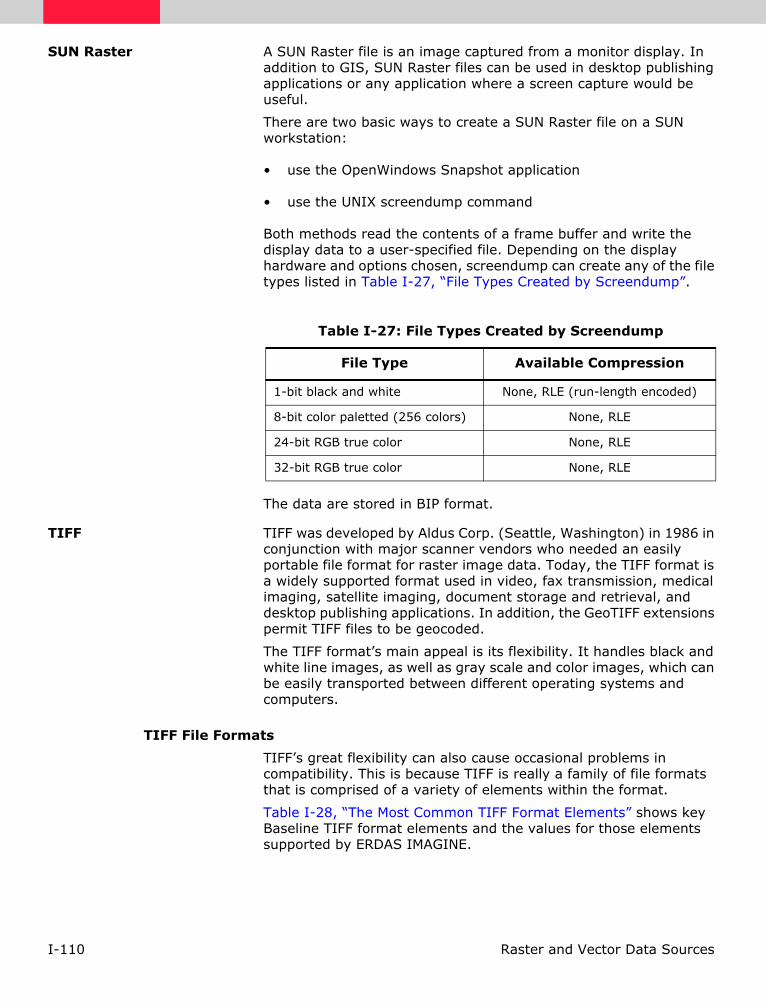
I-110 Raster and Vector Data Sources

SUN Raster A SUN Raster file is an image captured from a monitor display. In addition to GIS, SUN Raster files can be used in desktop publishing applications or any application where a screen capture would be useful.

There are two basic ways to create a SUN Raster file on a SUN workstation:

• use the OpenWindows Snapshot application

• use the UNIX screendump command

Both methods read the contents of a frame buffer and write the display data to a user-specified file. Depending on the display hardware and options chosen, screendump can create any of the file types listed in Table I-27, “File Types Created by Screendump”.

The data are stored in BIP format.

TIFF TIFF was developed by Aldus Corp. (Seattle, Washington) in 1986 in conjunction with major scanner vendors who needed an easily portable file format for raster image data. Today, the TIFF format is a widely supported format used in video, fax transmission, medical imaging, satellite imaging, document storage and retrieval, and desktop publishing applications. In addition, the GeoTIFF extensions permit TIFF files to be geocoded.

The TIFF format’s main appeal is its flexibility. It handles black and white line images, as well as gray scale and color images, which can be easily transported between different operating systems and computers.

TIFF File Formats

TIFF’s great flexibility can also cause occasional problems in compatibility. This is because TIFF is really a family of file formats that is comprised of a variety of elements within the format.

Table I-28, “The Most Common TIFF Format Elements” shows key Baseline TIFF format elements and the values for those elements supported by ERDAS IMAGINE.

Table I-27: File Types Created by Screendump

File Type Available Compression

1-bit black and white None, RLE (run-length encoded)

8-bit color paletted (256 colors) None, RLE

24-bit RGB true color None, RLE

32-bit RGB true color None, RLE

I-111Raster and Vector Data Sources

Any TIFF file that contains an unsupported value for one of these elements may not be compatible with ERDAS IMAGINE.

a All bands must contain the same number of bits (i.e., 4, 4, 4 or 8, 8, 8). Multiband data with bit depths differing per band cannot be imported into ERDAS IMAGINE.

b Must be imported and exported as 4-bit data.

c Direct read/write only.

d Compression supported on import and direct read/write only.

e LZW is governed by patents and is not supported by the basic version of ERDAS IMAGINE.

Table I-28: The Most Common TIFF Format Elements

Byte Order Intel (LSB/MSB)

Motorola (MSB/LSB)

Image Type Black and white

Gray scale

Inverted gray scale

Color palette

RGB (3-band)

Configuration BIP

BSQ

Bits Per Planea 1b, 2b, 4, 8, 16c, 32c, 64c

Compressiond None

CCITT G3 (B&W only)

CCITT G4 (B&W only)

Packbits

LZWe

LZW with horizontal differencinge

I-112 Raster and Vector Data Sources

GeoTIFF According to the GeoTIFF Format Specification, Revision 1.0, "The GeoTIFF spec defines a set of TIFF tags provided to describe all ’Cartographic’ information associated with TIFF imagery that originates from satellite imaging systems, scanned aerial photography, scanned maps, digital elevation models, or as a result of geographic analysis" ( Ritter and Ruth, 1995).

The GeoTIFF format separates cartographic information into two parts: georeferencing and geocoding.

Georeferencing

Georeferencing is the process of linking the raster space of an image to a model space (i.e., a map system). Raster space defines how the coordinate system grid lines are placed relative to the centers of the pixels of the image. In ERDAS IMAGINE, the grid lines of the coordinate system always intersect at the center of a pixel. GeoTIFF allows the raster space to be defined either as having grid lines intersecting at the centers of the pixels (PixelIsPoint) or as having grid lines intersecting at the upper left corner of the pixels (PixelIsArea). ERDAS IMAGINE converts the georeferencing values for PixelIsArea images so that they conform to its raster space definition.

GeoTIFF allows georeferencing via a scale and an offset, a full affine transformation, or a set of tie points. ERDAS IMAGINE currently ignores GeoTIFF georeferencing in the form of multiple tie points.

Geocoding

Geocoding is the process of linking coordinates in model space to the Earth’s surface. Geocoding allows for the specification of projection, datum, ellipsoid, etc. ERDAS IMAGINE interprets the GeoTIFF geocoding to determine the latitude and longitude of the map coordinates for GeoTIFF images. This interpretation also allows the GeoTIFF image to be reprojected.

In GeoTIFF, the units of the map coordinates are obtained from the geocoding, not from the georeferencing. In addition, GeoTIFF defines a set of standard projected coordinate systems. The use of a standard projected coordinate system in GeoTIFF constrains the units that can be used with that standard system. Therefore, if the units used with a projection in ERDAS IMAGINE are not equal to the implied units of an equivalent GeoTIFF geocoding, ERDAS IMAGINE transforms the georeferencing to conform to the implied units so that the standard projected coordinate system code can be used. The alternative (preserving the georeferencing as is and producing a nonstandard projected coordinate system) is regarded as less interoperable.

Vector Data from Other Software Vendors

It is possible to directly import several common vector formats into ERDAS IMAGINE. These files become vector layers when imported. These data can then be used for the analyses and, in most cases, exported back to their original format (if desired).

I-113Raster and Vector Data Sources

Although data can be converted from one type to another by importing a file into ERDAS IMAGINE and then exporting the ERDAS IMAGINE file into another format, the import and export routines were designed to work together. For example, if you have information in AutoCAD that you would like to use in the GIS, you can import a Drawing Interchange File (DXF) into ERDAS IMAGINE, do the analysis, and then export the data back to DXF format.

In most cases, attribute data are also imported into ERDAS IMAGINE. Each of the following sections lists the types of attribute data that are imported.

Use Import/Export to import vector data from other software vendors into ERDAS IMAGINE vector layers. These routines are based on ArcInfo data conversion routines.

See "Vector Data" for more information on ERDAS IMAGINE vector layers. See "Geographic Information Systems" for more information about using vector data in a GIS.

ARCGEN ARCGEN files are ASCII files created with the ArcInfo UNGENERATE command. The import ARCGEN program is used to import features to a new layer. Topology is not created or maintained, therefore the coverage must be built or cleaned after it is imported into ERDAS IMAGINE.

ARCGEN files must be properly prepared before they are imported into ERDAS IMAGINE. If there is a syntax error in the data file, the import process may not work. If this happens, you must kill the process, correct the data file, and then try importing again.

See the ArcInfo documentation for more information about these files.

AutoCAD (DXF) AutoCAD is a vector software package distributed by Autodesk, Inc. (Sausalito, California). AutoCAD is a computer-aided design program that enables the user to draw two- and three-dimensional models. This software is frequently used in architecture, engineering, urban planning, and many other applications.

AutoCAD DXF is the standard interchange format used by most CAD systems. The AutoCAD program DXFOUT creates a DXF file that can be converted to an ERDAS IMAGINE vector layer. AutoCAD files can also be output to IGES format using the AutoCAD program IGESOUT.

See "IGES" on page I-116 for more information about IGES files.

I-114 Raster and Vector Data Sources

DXF files can be converted in the ASCII or binary format. The binary format is an optional format for AutoCAD Releases 10 and 11. It is structured just like the ASCII format, only the data are in binary format.

DXF files are composed of a series of related layers. Each layer contains one or more drawing elements or entities. An entity is a drawing element that can be placed into an AutoCAD drawing with a single command. When converted to an ERDAS IMAGINE vector layer, each entity becomes a single feature. Table I-29, “Conversion of DXF Entries” describes how various DXF entities are converted to ERDAS IMAGINE.

The ERDAS IMAGINE import process also imports line and point attribute data (if they exist) and creates an INFO directory with the appropriate ACODE (arc attributes) and XCODE (point attributes) files. If an imported DXF file is exported back to DXF format, this information is also exported.

Refer to an AutoCAD manual for more information about the format of DXF files.

DLG DLGs are furnished by the U.S. Geological Survey and provide planimetric base map information, such as transportation, hydrography, contours, and public land survey boundaries. DLG files are available for the following USGS map series:

• 7.5- and 15-minute topographic quadrangles

• 1:100,000-scale quadrangles

Table I-29: Conversion of DXF Entries

DXF EntityERDAS

IMAGINEFeature

Comments

Line3DLine

Line These entities become two point lines. The initial Z value of 3D entities is stored.

TraceSolid

3DFace

Line These entities become four or five point lines. The initial Z value of 3D entities is stored.

CircleArc

Line These entities form lines. Circles are composed of 361 points—one vertex for each degree. The first and last point is at the same location.

Polyline Line These entities can be grouped to form a single line having many vertices.

PointShape

Point These entities become point features in a layer.

I-115Raster and Vector Data Sources

• 1:2,000,000-scale national atlas maps

DLGs are topological files that contain nodes, lines, and areas (similar to the points, lines, and polygons in an ERDAS IMAGINE vector layer). DLGs also store attribute information in the form of major and minor code pairs. Code pairs are encoded in two integer fields, each containing six digits. The major code describes the class of the feature (road, stream, etc.) and the minor code stores more specific information about the feature.

DLGs can be imported in standard format (144 bytes per record) and optional format (80 bytes per record). You can export to DLG-3 optional format. Most DLGs are in the Universal Transverse Mercator (UTM) map projection. However, the 1:2,000,000 scale series is in geographic coordinates.

The ERDAS IMAGINE import process also imports point, line, and polygon attribute data (if they exist) and creates an INFO directory with the appropriate ACODE, PCODE (polygon attributes), and XCODE files. If an imported DLG file is exported back to DLG format, this information is also exported.

To maintain the topology of a vector layer created from a DLG file, you must Build or Clean it. See "Geographic Information Systems" for information on this process.

ETAK ETAK’s MapBase is an ASCII digital street centerline map product available from ETAK, Inc. (Menlo Park, California). ETAK files are similar in content to the Dual Independent Map Encoding (DIME) format used by the U.S. Census Bureau. Each record represents a single linear feature with address and political, census, and ZIP code boundary information. ETAK has also included road class designations and, in some areas, major landmark features.

There are four possible types of ETAK features:

• DIME or D types—if the feature type is D, a line is created along with a corresponding ACODE (arc attribute) record. The coordinates are stored in Lat/Lon decimal degrees.

• Alternate address or A types—each record contains an alternate address record for a line. These records are written to the attribute file, and are useful for building address coverages.

• Shape features or S types—shape records are used to add vertices to the lines. The coordinates for these features are in Lat/Lon decimal degrees.

• Landmark or L types—if the feature type is L and you opt to output a landmark layer, then a point feature is created along with an associated PCODE record.

I-116 Raster and Vector Data Sources

ERDAS IMAGINE vector data cannot be exported to ETAK format.

IGES IGES files are often used to transfer CAD data between systems. IGES Version 3.0 format, published by the U.S. Department of Commerce, is in uncompressed ASCII format only.

IGES files can be produced in AutoCAD using the IGESOUT command. The following IGES entities can be converted:

The ERDAS IMAGINE import process also imports line and point attribute data (if they exist) and creates an INFO directory with the appropriate ACODE and XCODE files. If an imported IGES file is exported back to IGES format, this information is also exported.

TIGER TIGER files are line network products of the U.S. Census Bureau. The Census Bureau is using the TIGER system to create and maintain a digital cartographic database that covers the United States, Puerto Rico, Guam, the Virgin Islands, American Samoa, and the Trust Territories of the Pacific.

TIGER/Line is the line network product of the TIGER system. The cartographic base is taken from Geographic Base File/Dual Independent Map Encoding (GBF/DIME), where available, and from the USGS 1:100,000-scale national map series, SPOT imagery, and a variety of other sources in all other areas, in order to have continuous coverage for the entire United States. In addition to line segments, TIGER files contain census geographic codes and, in metropolitan areas, address ranges for the left and right sides of each segment. TIGER files are available in ASCII format on both CD-ROM and tape media. All released versions after April 1989 are supported.

There is a great deal of attribute information provided with TIGER/Line files. Line and point attribute information can be converted into ERDAS IMAGINE format. The ERDAS IMAGINE import process creates an INFO directory with the appropriate ACODE and XCODE files. If an imported TIGER file is exported back to TIGER format, this information is also exported.

TIGER attributes include the following:

Table I-30: Conversion of IGES Entities

IGES Entity ERDAS IMAGINE Feature

IGES Entity 100 (Circular Arc Entities) Lines

IGES Entity 106 (Copious Data Entities) Lines

IGES Entity 106 (Line Entities) Lines

IGES Entity 116 (Point Entities) Points

I-117Raster and Vector Data Sources

• Version numbers—TIGER/Line file version number.

• Permanent record numbers—each line segment is assigned a permanent record number that is maintained throughout all versions of TIGER/Line files.

• Source codes—each line and landmark point feature is assigned a code to specify the original source.

• Census feature class codes—line segments representing physical features are coded based on the USGS classification codes in DLG-3 files.

• Street attributes—includes street address information for selected urban areas.

• Legal and statistical area attributes—legal areas include states, counties, townships, towns, incorporated cities, Indian reservations, and national parks. Statistical areas are areas used during the census-taking, where legal areas are not adequate for reporting statistics.

• Political boundaries—the election precincts or voting districts may contain a variety of areas, including wards, legislative districts, and election districts.

• Landmarks—landmark area and point features include schools, military installations, airports, hospitals, mountain peaks, campgrounds, rivers, and lakes.

TIGER files for major metropolitan areas outside of the United States (e.g., Puerto Rico, Guam) do not have address ranges.

Disk Space Requirements

TIGER/Line files are partitioned into counties ranging in size from less than a megabyte to almost 120 megabytes. The average size is approximately 10 megabytes. To determine the amount of disk space required to convert a set of TIGER/Line files, use this rule: the size of the converted layers is approximately the same size as the files used in the conversion. The amount of additional scratch space needed depends on the largest file and whether it needs to be sorted. The amount usually required is about double the size of the file being sorted.

The information presented in this section, “Vector Data from Other Software Vendors” on page I-112, was obtained from the Data Conversion and the 6.0 ARC Command References manuals, both published by ESRI, Inc., 1992.

I-118 Raster and Vector Data Sources

I-117Image Display

Image Display

Introduction This section defines some important terms that are relevant to image display. Most of the terminology and definitions used in this chapter are based on the X Window System (Massachusetts Institute of Technology) terminology. This may differ from other systems, such as Microsoft Windows NT.

A seat is a combination of an X-server and a host workstation.

• A host workstation consists of a CPU, keyboard, mouse, and a display.

• A display may consist of multiple screens. These screens work together, making it possible to move the mouse from one screen to the next.

• The display hardware contains the memory that is used to produce the image. This hardware determines which types of displays are available (e.g., true color or pseudo color) and the pixel depth (e.g., 8-bit or 24-bit).

Figure I-35: Example of One Seat with One Display and Two Screens

Display Memory Size The size of memory varies for different displays. It is expressed in terms of:

• display resolution, which is expressed as the horizontal and vertical dimensions of memory—the number of pixels that can be viewed on the display screen. Some typical display resolutions are 1152 × 900, 1280× 1024, and 1024 × 780. For the PC, typical resolutions are 640 × 480, 800 × 600, 1024 × 768, and 1280 × 1024, and

• the number of bits for each pixel or pixel depth, as explained below.

Screen Screen

I-118 Image Display

Bits for Image Plane

A bit is a binary digit, meaning a number that can have two possible values—0 and 1, or off and on. A set of bits, however, can have many more values, depending upon the number of bits used. The number of values that can be expressed by a set of bits is 2 to the power of the number of bits used. For example, the number of values that can be expressed by 3 bits is 8 (23 = 8).

Displays are referred to in terms of a number of bits, such as 8-bit or 24-bit. These bits are used to determine the number of possible brightness values. For example, in a 24-bit display, 24 bits per pixel breaks down to eight bits for each of the three color guns per pixel. The number of possible values that can be expressed by eight bits is 28, or 256. Therefore, on a 24-bit display, each color gun of a pixel can have any one of 256 possible brightness values, expressed by the range of values 0 to 255.

The combination of the three color guns, each with 256 possible brightness values, yields 2563, (or 224, for the 24-bit image display), or 16,777,216 possible colors for each pixel on a 24-bit display. If the display being used is not 24-bit, the example above calculates the number of possible brightness values and colors that can be displayed.

Pixel The term pixel is abbreviated from picture element. As an element, a pixel is the smallest part of a digital picture (image). Raster image data are divided by a grid, in which each cell of the grid is represented by a pixel. A pixel is also called a grid cell.

Pixel is a broad term that is used for both:

• the data file value(s) for one data unit in an image (file pixels), or

• one grid location on a display or printout (display pixels).

Usually, one pixel in a file corresponds to one pixel in a display or printout. However, an image can be magnified or reduced so that one file pixel no longer corresponds to one pixel in the display or printout. For example, if an image is displayed with a magnification factor of 2, then one file pixel takes up 4 (2 × 2) grid cells on the display screen.

To display an image, a file pixel that consists of one or more numbers must be transformed into a display pixel with properties that can be seen, such as brightness and color. Whereas the file pixel has values that are relevant to data (such as wavelength of reflected light), the displayed pixel must have a particular color or gray level that represents these data file values.

Colors Human perception of color comes from the relative amounts of red, green, and blue light that are measured by the cones (sensors) in the eye. Red, green, and blue light can be added together to produce a wide variety of colors—a wider variety than can be formed from the combinations of any three other colors. Red, green, and blue are therefore the additive primary colors.

I-119Image Display

A nearly infinite number of shades can be produced when red, green, and blue light are combined. On a display, different colors (combinations of red, green, and blue) allow you to perceive changes across an image. Color displays that are available today yield 224, or 16,777,216 colors. Each color has a possible 256 different values (28).

Color Guns

On a display, color guns direct electron beams that fall on red, green, and blue phosphors. The phosphors glow at certain frequencies to produce different colors. Color monitors are often called RGB monitors, referring to the primary colors.

The red, green, and blue phosphors on the picture tube appear as tiny colored dots on the display screen. The human eye integrates these dots together, and combinations of red, green, and blue are perceived. Each pixel is represented by an equal number of red, green, and blue phosphors.

Brightness Values

Brightness values (or intensity values) are the quantities of each primary color to be output to each displayed pixel. When an image is displayed, brightness values are calculated for all three color guns, for every pixel.

All of the colors that can be output to a display can be expressed with three brightness values—one for each color gun.

Colormap and Colorcells A color on the screen is created by a combination of red, green, and blue values, where each of these components is represented as an 8-bit value. Therefore, 24 bits are needed to represent a color. Since many systems have only an 8-bit display, a colormap is used to translate the 8-bit value into a color. A colormap is an ordered set of colorcells, which is used to perform a function on a set of input values. To display or print an image, the colormap translates data file values in memory into brightness values for each color gun. Colormaps are not limited to 8-bit displays.

Colormap vs. Lookup Table

The colormap is a function of the display hardware, whereas a lookup table is a function of ERDAS IMAGINE. When a contrast adjustment is performed on an image in ERDAS IMAGINE, lookup tables are used. However, if the auto-update function is being used to view the adjustments in near real-time, then the colormap is being used to map the image through the lookup table. This process allows the colors on the screen to be updated in near real-time. This chapter explains how the colormap is used to display imagery.

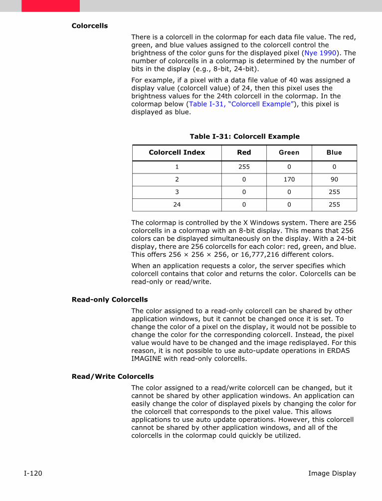
I-120 Image Display

Colorcells

There is a colorcell in the colormap for each data file value. The red, green, and blue values assigned to the colorcell control the brightness of the color guns for the displayed pixel (Nye 1990). The number of colorcells in a colormap is determined by the number of bits in the display (e.g., 8-bit, 24-bit).

For example, if a pixel with a data file value of 40 was assigned a display value (colorcell value) of 24, then this pixel uses the brightness values for the 24th colorcell in the colormap. In the colormap below (Table I-31, “Colorcell Example”), this pixel is displayed as blue.

The colormap is controlled by the X Windows system. There are 256 colorcells in a colormap with an 8-bit display. This means that 256 colors can be displayed simultaneously on the display. With a 24-bit display, there are 256 colorcells for each color: red, green, and blue. This offers 256 × 256 × 256, or 16,777,216 different colors.

When an application requests a color, the server specifies which colorcell contains that color and returns the color. Colorcells can be read-only or read/write.

Read-only Colorcells

The color assigned to a read-only colorcell can be shared by other application windows, but it cannot be changed once it is set. To change the color of a pixel on the display, it would not be possible to change the color for the corresponding colorcell. Instead, the pixel value would have to be changed and the image redisplayed. For this reason, it is not possible to use auto-update operations in ERDAS IMAGINE with read-only colorcells.

Read/Write Colorcells

The color assigned to a read/write colorcell can be changed, but it cannot be shared by other application windows. An application can easily change the color of displayed pixels by changing the color for the colorcell that corresponds to the pixel value. This allows applications to use auto update operations. However, this colorcell cannot be shared by other application windows, and all of the colorcells in the colormap could quickly be utilized.

Table I-31: Colorcell Example

Colorcell Index Red Green Blue

1 255 0 0

2 0 170 90

3 0 0 255

24 0 0 255

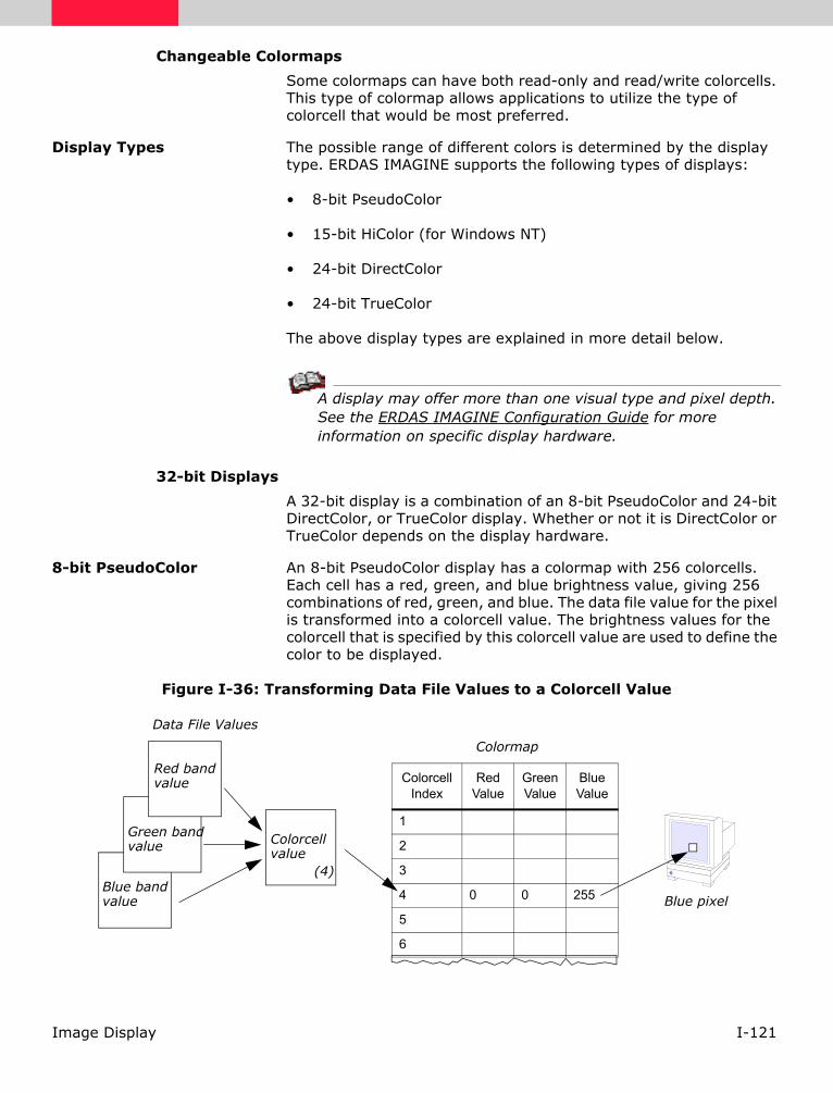
I-121Image Display

Changeable Colormaps

Some colormaps can have both read-only and read/write colorcells. This type of colormap allows applications to utilize the type of colorcell that would be most preferred.

Display Types The possible range of different colors is determined by the display type. ERDAS IMAGINE supports the following types of displays:

• 8-bit PseudoColor

• 15-bit HiColor (for Windows NT)

• 24-bit DirectColor

• 24-bit TrueColor

The above display types are explained in more detail below.

A display may offer more than one visual type and pixel depth. See the ERDAS IMAGINE Configuration Guide for more information on specific display hardware.

32-bit Displays

A 32-bit display is a combination of an 8-bit PseudoColor and 24-bit DirectColor, or TrueColor display. Whether or not it is DirectColor or TrueColor depends on the display hardware.

8-bit PseudoColor An 8-bit PseudoColor display has a colormap with 256 colorcells. Each cell has a red, green, and blue brightness value, giving 256 combinations of red, green, and blue. The data file value for the pixel is transformed into a colorcell value. The brightness values for the colorcell that is specified by this colorcell value are used to define the color to be displayed.

Figure I-36: Transforming Data File Values to a Colorcell Value

Colorcell Index

RedValue

Green Value

BlueValue

1

2

3

4 0 0 255

5

6

Red bandvalue

Green bandvalue

Blue bandvalue

Colorcell value

(4)

Data File Values

Colormap

Blue pixel

I-122 Image Display

In Figure I-36, data file values for a pixel of three continuous raster layers (bands) is transformed to a colorcell value. Since the colorcell value is four, the pixel is displayed with the brightness values of the fourth colorcell (blue).

This display grants a small number of colors to ERDAS IMAGINE. It works well with thematic raster layers containing less than 200 colors and with gray scale continuous raster layers. For image files with three continuous raster layers (bands), the colors are severely limited because, under ideal conditions, 256 colors are available on an 8-bit display, while 8-bit, 3-band image files can contain over 16,000,000 different colors.

Auto Update

An 8-bit PseudoColor display has read-only and read/write colorcells, allowing ERDAS IMAGINE to perform near real-time color modifications using Auto Update and Auto Apply options.

24-bit DirectColor A 24-bit DirectColor display enables you to view up to three bands of data at one time, creating displayed pixels that represent the relationships between the bands by their colors. Since this is a 24-bit display, it offers up to 256 shades of red, 256 shades of green, and 256 shades of blue, which is approximately 16 million different colors (2563). The data file values for each band are transformed into colorcell values. The colorcell that is specified by these values is used to define the color to be displayed.

I-123Image Display

Figure I-37: Transforming Data File Values to a Colorcell Value

In Figure I-37, data file values for a pixel of three continuous raster layers (bands) are transformed to separate colorcell values for each band. Since the colorcell value is 1 for the red band, 2 for the green band, and 6 for the blue band, the RGB brightness values are 0, 90, 200. This displays the pixel as a blue-green color.

This type of display grants a very large number of colors to ERDAS IMAGINE and it works well with all types of data.

Auto Update

A 24-bit DirectColor display has read-only and read/write colorcells, allowing ERDAS IMAGINE to perform real-time color modifications using the Auto Update and Auto Apply options.

24-bit TrueColor A 24-bit TrueColor display enables you to view up to three continuous raster layers (bands) of data at one time, creating displayed pixels that represent the relationships between the bands by their colors. The data file values for the pixels are transformed into screen values and the colors are based on these values. Therefore, the color for the pixel is calculated without querying the server and the colormap. The colormap for a 24-bit TrueColor display is not available for ERDAS IMAGINE applications. Once a color is assigned to a screen value, it cannot be changed, but the color can be shared by other applications.

Red band value

Green band value

Blue band value

Data File Values

Red band value

Green band value

Blue band value

Colorcell Values

(1)

(2)

(6)

Blue-green pixel (0, 90, 200 RGB)

Colormap

Color- Cell Index

1

2

3

4

5

6

Blue Value

0

0

200

Color- Cell Index

Green Value

Red Value

Color- Cell Index

1

2

3

4

5

6

0

90

55

1

2

3

4

5

6

0

0

55

I-124 Image Display

The screen values are used as the brightness values for the red, green, and blue color guns. Since this is a 24-bit display, it offers 256 shades of red, 256 shades of green, and 256 shades of blue, which is approximately 16 million different colors (2563).

Figure I-38: Transforming Data File Values to Screen Values

In Figure I-38, data file values for a pixel of three continuous raster layers (bands) are transformed to separate screen values for each band. Since the screen value is 0 for the red band, 90 for the green band, and 200 for the blue band, the RGB brightness values are 0, 90, and 200. This displays the pixel as a blue-green color.

Auto Update

The 24-bit TrueColor display does not use the colormap in ERDAS IMAGINE, and thus does not provide ERDAS IMAGINE with any real-time color changing capability. Each time a color is changed, the screen values must be calculated and the image must be redrawn.

Color Quality

The 24-bit TrueColor visual provides the best color quality possible with standard equipment. There is no color degradation under any circumstances with this display.

PC Displays ERDAS IMAGINE for Microsoft Windows NT supports the following visual type and pixel depths:

• 8-bit PseudoColor

• 15-bit HiColor

• 24-bit TrueColor

Red band value

Green band value

Blue band value

Data File Values

Red band value

Green band value

Blue band value

Screen Values

(0)

(90)

(200)

Blue-green pixel (0, 90, 200 RGB)

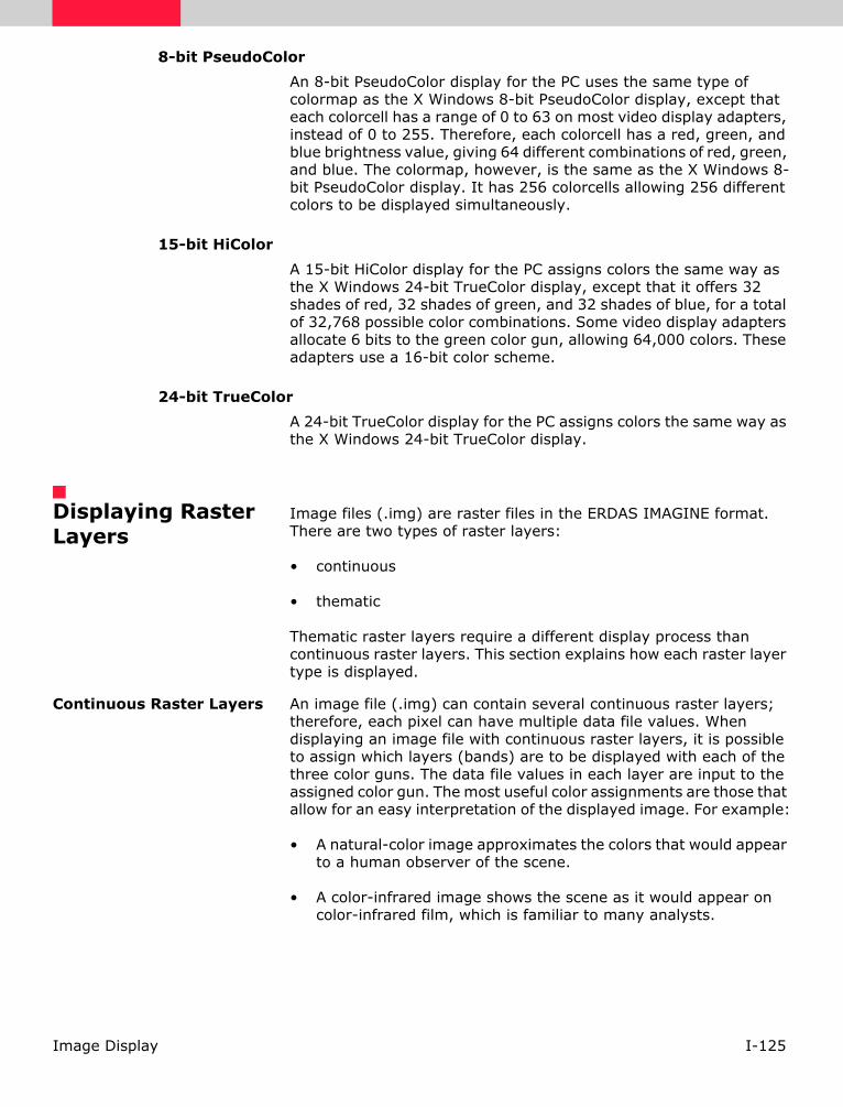
I-125Image Display

8-bit PseudoColor

An 8-bit PseudoColor display for the PC uses the same type of colormap as the X Windows 8-bit PseudoColor display, except that each colorcell has a range of 0 to 63 on most video display adapters, instead of 0 to 255. Therefore, each colorcell has a red, green, and blue brightness value, giving 64 different combinations of red, green, and blue. The colormap, however, is the same as the X Windows 8-bit PseudoColor display. It has 256 colorcells allowing 256 different colors to be displayed simultaneously.

15-bit HiColor

A 15-bit HiColor display for the PC assigns colors the same way as the X Windows 24-bit TrueColor display, except that it offers 32 shades of red, 32 shades of green, and 32 shades of blue, for a total of 32,768 possible color combinations. Some video display adapters allocate 6 bits to the green color gun, allowing 64,000 colors. These adapters use a 16-bit color scheme.

24-bit TrueColor

A 24-bit TrueColor display for the PC assigns colors the same way as the X Windows 24-bit TrueColor display.

Displaying Raster Layers

Image files (.img) are raster files in the ERDAS IMAGINE format. There are two types of raster layers:

• continuous

• thematic

Thematic raster layers require a different display process than continuous raster layers. This section explains how each raster layer type is displayed.

Continuous Raster Layers An image file (.img) can contain several continuous raster layers; therefore, each pixel can have multiple data file values. When displaying an image file with continuous raster layers, it is possible to assign which layers (bands) are to be displayed with each of the three color guns. The data file values in each layer are input to the assigned color gun. The most useful color assignments are those that allow for an easy interpretation of the displayed image. For example:

• A natural-color image approximates the colors that would appear to a human observer of the scene.

• A color-infrared image shows the scene as it would appear on color-infrared film, which is familiar to many analysts.

I-126 Image Display

Band assignments are often expressed in R,G,B order. For example, the assignment 4, 2, 1 means that band 4 is assigned to red, band 2 to green, and band 1 to blue. Below are some widely used band to color gun assignments ( Faust, 1989):

• Landsat TM—natural color: 3, 2, 1This is natural color because band 3 is red and is assigned to the red color gun, band 2 is green and is assigned to the green color gun, and band 1 is blue and is assigned to the blue color gun.

• Landsat TM—color-infrared: 4, 3, 2This is infrared because band 4 = infrared.

• SPOT Multispectral—color-infrared: 3, 2, 1This is infrared because band 3 = infrared.

Contrast Table

When an image is displayed, ERDAS IMAGINE automatically creates a contrast table for continuous raster layers. The red, green, and blue brightness values for each band are stored in this table.

Since the data file values in continuous raster layers are quantitative and related, the brightness values in the colormap are also quantitative and related. The screen pixels represent the relationships between the values of the file pixels by their colors. For example, a screen pixel that is bright red has a high brightness value in the red color gun, and a high data file value in the layer assigned to red, relative to other data file values in that layer.

The brightness values often differ from the data file values, but they usually remain in the same order of lowest to highest. Some meaningful relationships between the values are usually maintained.

Contrast Stretch

Different displays have different ranges of possible brightness values. The range of most displays is 0 to 255 for each color gun.

Since the data file values in a continuous raster layer often represent raw data (such as elevation or an amount of reflected light), the range of data file values is often not the same as the range of brightness values of the display. Therefore, a contrast stretch is usually performed, which stretches the range of the values to fit the range of the display.

For example, Figure I-39 shows a layer that has data file values from 30 to 40. When these values are used as brightness values, the contrast of the displayed image is poor. A contrast stretch simply stretches the range between the lower and higher data file values, so that the contrast of the displayed image is higher—that is, lower data file values are displayed with the lowest brightness values, and higher data file values are displayed with the highest brightness values.

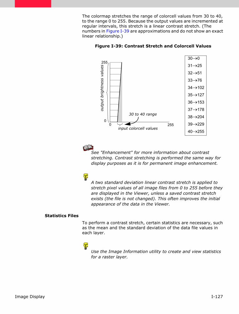
I-127Image Display

The colormap stretches the range of colorcell values from 30 to 40, to the range 0 to 255. Because the output values are incremented at regular intervals, this stretch is a linear contrast stretch. (The numbers in Figure I-39 are approximations and do not show an exact linear relationship.)

Figure I-39: Contrast Stretch and Colorcell Values

See "Enhancement" for more information about contrast stretching. Contrast stretching is performed the same way for display purposes as it is for permanent image enhancement.

A two standard deviation linear contrast stretch is applied to stretch pixel values of all image files from 0 to 255 before they are displayed in the Viewer, unless a saved contrast stretch exists (the file is not changed). This often improves the initial appearance of the data in the Viewer.

Statistics Files

To perform a contrast stretch, certain statistics are necessary, such as the mean and the standard deviation of the data file values in each layer.

Use the Image Information utility to create and view statistics for a raster layer.

input colorcell values

outp

ut

brightn

ess

valu

es

255

25500

30 to 40 range

30→0

31→25

32→51

33→76

34→102

35→127

36→153

37→178

38→204

39→229

40→255

I-128 Image Display

Usually, not all of the data file values are used in the contrast stretch calculations. The minimum and maximum data file values of each band are often too extreme to produce good results. When the minimum and maximum are extreme in relation to the rest of the data, then the majority of data file values are not stretched across a very wide range, and the displayed image has low contrast.

Figure I-40: Stretching by Min/Max vs. Standard Deviation

The mean and standard deviation of the data file values for each band are used to locate the majority of the data file values. The number of standard deviations above and below the mean can be entered, which determines the range of data used in the stretch.

See "Math Topics" on page II-243 for more information on mean and standard deviation.

Use the Contrast Tools dialog, which is accessible from the Lookup Table Modification dialog, to enter the number of standard deviations to be used in the contrast stretch.

24-bit DirectColor and TrueColor Displays

Figure I-41 illustrates the general process of displaying three continuous raster layers on a 24-bit DirectColor display. The process is similar on a TrueColor display except that the colormap is not used.

0 255-2σ mean +2σ

stretched data file values

frequ

ency

most of the data

Standard Deviation Stretch

values stretchedover 255 are not displayed

values stretchedless than 0 are

not displayed

Original Histogram

0 255-2σ mean +2σstored data file values

frequ

ency

0 255-2σ mean +2σstretched data file values

frequ

ency

most of the data

Min/Max Stretch

I-129Image Display

Figure I-41: Continuous Raster Layer Display Process

8-bit PseudoColor Display

When displaying continuous raster layers on an 8-bit PseudoColor display, the data file values from the red, green, and blue bands are combined and transformed to a colorcell value in the colormap. This colorcell then provides the red, green, and blue brightness values. Since there are only 256 colors available, a continuous raster layer looks different when it is displayed in an 8-bit display than a 24-bit display that offers 16 million different colors. However, the Viewer performs dithering with the available colors in the colormap to let a smaller set of colors appear to be a larger set of colors.

See "Dithering" on page I-137 for more information.

Band-to- color gun assignments:

Histograms

Ranges of data file values to be displayed:

Colormap:

Color guns:

Brightness values in each color gun:

Color display:

Band 3 assigned to

RED

Band 2 assigned to

GREEN

Band 1 assigned to

BLUE

data file values in

of each band:

brightness values out brightness values out brightness values out

0 255 0 255 0 255

data file values in data file values in

0 255 0 255 0 255

0 255 0 255 0 255

I-130 Image Display

Thematic Raster Layers A thematic raster layer generally contains pixels that have been classified, or put into distinct categories. Each data file value is a class value, which is simply a number for a particular category. A thematic raster layer is stored in an image (.img) file. Only one data file value—the class value—is stored for each pixel.

Since these class values are not necessarily related, the gradations that are possible in true color mode are not usually useful in pseudo color. The class system gives the thematic layer a discrete look, in which each class can have its own color.

Color Table

When a thematic raster layer is displayed, ERDAS IMAGINE automatically creates a color table. The red, green, and blue brightness values for each class are stored in this table.

RGB Colors

Individual color schemes can be created by combining red, green, and blue in different combinations, and assigning colors to the classes of a thematic layer.

Colors can be expressed numerically, as the brightness values for each color gun. Brightness values of a display generally range from 0 to 255, however, ERDAS IMAGINE translates the values from 0 to 1. The maximum brightness value for the display device is scaled to 1. The colors listed in Table I-32, “Commonly Used RGB Colors” are based on the range that is used to assign brightness values in ERDAS IMAGINE.

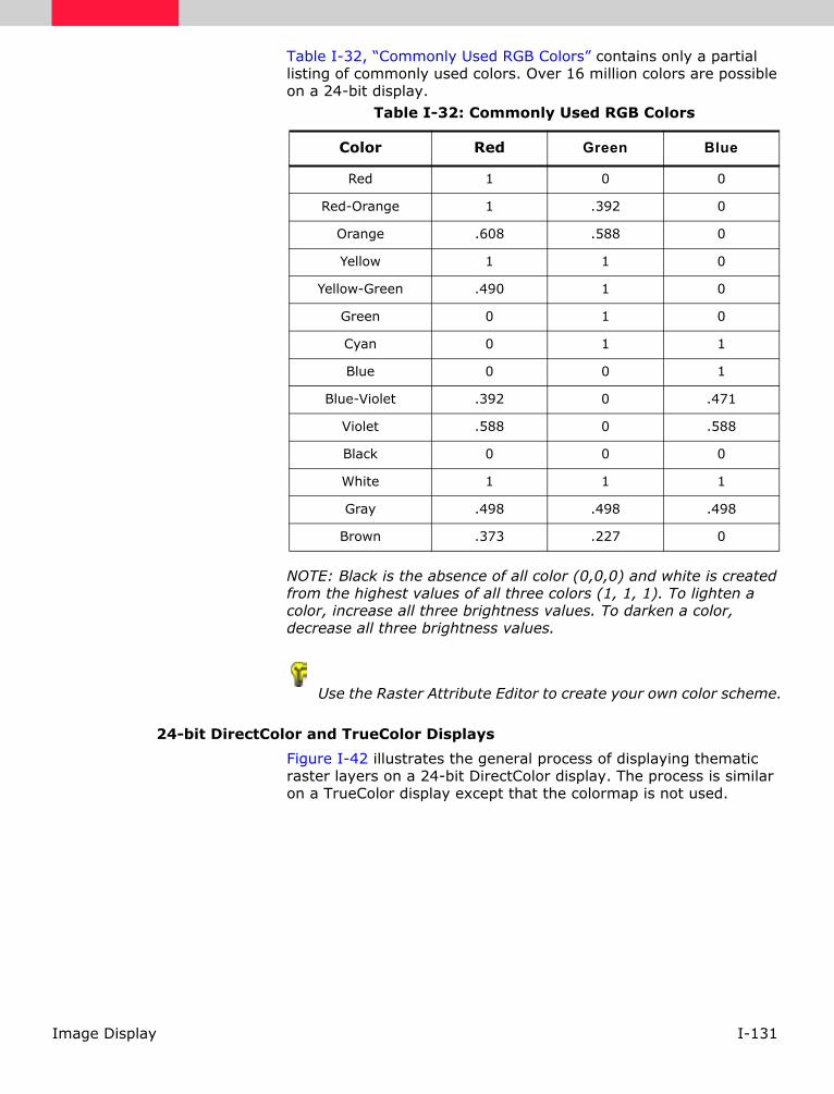
I-131Image Display

Table I-32, “Commonly Used RGB Colors” contains only a partial listing of commonly used colors. Over 16 million colors are possible on a 24-bit display.

NOTE: Black is the absence of all color (0,0,0) and white is created from the highest values of all three colors (1, 1, 1). To lighten a color, increase all three brightness values. To darken a color, decrease all three brightness values.

Use the Raster Attribute Editor to create your own color scheme.

24-bit DirectColor and TrueColor Displays

Figure I-42 illustrates the general process of displaying thematic raster layers on a 24-bit DirectColor display. The process is similar on a TrueColor display except that the colormap is not used.

Table I-32: Commonly Used RGB Colors

Color Red Green Blue

Red 1 0 0

Red-Orange 1 .392 0

Orange .608 .588 0

Yellow 1 1 0

Yellow-Green .490 1 0

Green 0 1 0

Cyan 0 1 1

Blue 0 0 1

Blue-Violet .392 0 .471

Violet .588 0 .588

Black 0 0 0

White 1 1 1

Gray .498 .498 .498

Brown .373 .227 0

I-132 Image Display

Figure I-42: Thematic Raster Layer Display Process

Display a thematic raster layer from the Viewer.

8-bit PseudoColor Display

The colormap is a limited resource that is shared among all of the applications that are running concurrently. Because of the limited resources, ERDAS IMAGINE does not typically have access to the entire colormap.

1 2 3

4 3 5

2 1 4

Colormap:

Color guns:

Brightness values in each color gun:

Display:

class values in

brightness values out brightness values out brightness values out

class values in class values in1 2 3 4 51 2 3 4 5 1 2 3 4 5

0 128 255 0 128 255 0 128 255

R O Y

V Y G

O R V

= 255= 128= 0

Original image by class:

Colorscheme:

CLASS12345

COLORRed =Orange =Yellow =Violet =Green =

RED2552552551280

GREEN01282550255

BLUE0002550

Brightness Values

I-133Image Display

Using the Viewer The Viewer is a window for displaying raster, vector, and annotation layers. You can open as many Viewer windows as their window manager supports.

NOTE: The more Viewers that are opened simultaneously, the more RAM memory is necessary.

The Viewer not only makes digital images visible quickly, but it can also be used as a tool for image processing and raster GIS modeling. The uses of the Viewer are listed briefly in this section, and described in greater detail in other chapters of the ERDAS Field Guide.

Colormap

ERDAS IMAGINE does not use the entire colormap because there are other applications that also need to use it, including the window manager, terminal windows, Arc View, or a clock. Therefore, there are some limitations to the number of colors that the Viewer can display simultaneously, and flickering may occur as well.

Color Flickering

If an application requests a new color that does not exist in the colormap, the server assigns that color to an empty colorcell. However, if there are not any available colorcells and the application requires a private colorcell, then a private colormap is created for the application window. Since this is a private colormap, when the cursor is moved out of the window, the server uses the main colormap and the brightness values assigned to the colorcells. Therefore, the colors in the private colormap are not applied and the screen flickers. Once the cursor is moved into the application window, the correct colors are applied for that window.

Resampling

When a raster layer(s) is displayed, the file pixels may be resampled for display on the screen. Resampling is used to calculate pixel values when one raster grid must be fitted to another. In this case, the raster grid defined by the file must be fit to the grid of screen pixels in the Viewer.

All Viewer operations are file-based. So, any time an image is resampled in the Viewer, the Viewer uses the file as its source. If the raster layer is magnified or reduced, the Viewer refits the file grid to the new screen grid.

The resampling methods available are:

• Nearest Neighbor—uses the value of the closest pixel to assign to the output pixel value.

• Bilinear Interpolation—uses the data file values of four pixels in a 2 × 2 window to calculate an output value with a bilinear function.

I-134 Image Display

• Cubic Convolution—uses the data file values of 16 pixels in a 4 × 4 window to calculate an output value with a cubic function.

These are discussed in detail in "Rectification" on page I-219.

The default resampling method is Nearest Neighbor.

Preference Editor

The Preference Editor enables you to set parameters for the Viewer that affect the way the Viewer operates.

See the ERDAS IMAGINE On-Line Help for the Preference Editor for information on how to set preferences for the Viewer.

Pyramid Layers Sometimes a large image file may take a long time to display in the Viewer or to be resampled by an application. The Pyramid Layer option enables you to display large images faster and allows certain applications to rapidly access the resampled data. Pyramid layers are image layers which are copies of the original layer successively reduced by the power of 2 and then resampled. If the raster layer is thematic, then it is resampled using the Nearest Neighbor method. If the raster layer is continuous, it is resampled by a method that is similar to Cubic Convolution. The data file values for sixteen pixels in a 4 × 4 window are used to calculate an output data file value with a filter function.

See "Rectification" on page I-219 for more information on Nearest Neighbor.

The number of pyramid layers created depends on the size of the original image. A larger image produces more pyramid layers. When the Create Pyramid Layer option is selected, ERDAS IMAGINE automatically creates successively reduced layers until the final pyramid layer can be contained in one block. The default block size is 64 × 64 pixels.

See "Raster Data" on page I-1 for information on block size.

Pyramid layers are added as additional layers in the image file. However, these layers cannot be accessed for display. The file size is increased by approximately one-third when pyramid layers are created. The actual increase in file size can be determined by multiplying the layer size by this formula

I-135Image Display

Where:

n = number of pyramid layers

NOTE: This equation is applicable to all types of pyramid layers: internal and external.

Pyramid layers do not appear as layers which can be processed: they are for viewing purposes only. Therefore, they do not appear as layers in other parts of the ERDAS IMAGINE system (e.g., the Arrange Layers dialog).

The Image Files (General) section of the Preference Editor contains a preference for the Initial Pyramid Layer Number. By default, the value is set to 2. This means that the first pyramid layer generated is discarded. In Figure I-43 below, the 2K × 2K layer is discarded. If you wish to keep that layer, then set the Initial Pyramid Layer Number to 1.

Pyramid layers can be deleted through the Image Information utility. However, when pyramid layers are deleted, they are not deleted from the image file; therefore, the image file size does not change, but ERDAS IMAGINE utilizes this file space, if necessary. Pyramid layers are deleted from viewing and resampling access only - that is, they can no longer be viewed or used in an application.

14i----

i 0=

n

∑

I-136 Image Display

Figure I-43: Pyramid Layers

For example, a file that is 4K × 4K pixels could take a long time to display when the image is fit to the Viewer. The Compute Pyramid Layers option creates additional layers successively reduced from 4K × 4K, to 2K × 2K, 1K × 1K, 512 × 512, 128 × 128, down to 64 × 64. ERDAS IMAGINE then selects the pyramid layer size most appropriate for display in the Viewer window when the image is displayed.

The Compute Pyramid Layers option is available from Import and the Image Information utility.

For more information about the .img format, see "Raster Data" on page I-1 and the On-Line Help.

External Pyramid Layers

Pyramid layers can be either internal or external. If you choose external pyramid layers, they are stored with the same name in the same directory as the image with which they are associated, but with the .rrd extension. For example, an image named tm_image1.img has external pyramid layers contained in a file named tm_image1.rrd.

Original Image

Pyramid layer (2K × 2K)

Pyramid layer (1K × 1K)

Pyramid layer (512 × 512)

Pyramid layer (128 × 128)

Pyramid layer (64 × 64)

image file

ERDAS IMAGINE selects the pyramid layer that displays the fastest in the Viewer.

Viewer Window

(4K × 4K)

I-137Image Display

The extension .rrd stands for reduced resolution data set. You can delete the external pyramid layers associated with an image by accessing the Image Information dialog. Unlike internal pyramid layers, external pyramid layers do not affect the size of the associated image.

Dithering A display is capable of viewing only a limited number of colors simultaneously. For example, an 8-bit display has a colormap with 256 colorcells, therefore, a maximum of 256 colors can be displayed at the same time. If some colors are being used for auto update color adjustment while other colors are still being used for other imagery, the color quality degrades.

Dithering lets a smaller set of colors appear to be a larger set of colors. If the desired display color is not available, a dithering algorithm mixes available colors to provide something that looks like the desired color.

For a simple example, assume the system can display only two colors: black and white, and you want to display gray. This can be accomplished by alternating the display of black and white pixels.

Figure I-44: Example of Dithering

In Figure I-44, dithering is used between a black pixel and a white pixel to obtain a gray pixel.

The colors that the Viewer dithers between are similar to each other, and are dithered on the pixel level. Using similar colors and dithering on the pixel level makes the image appear smooth.

Dithering allows multiple images to be displayed in different Viewers without refreshing the currently displayed image(s) each time a new image is displayed.

Color Patches

When the Viewer performs dithering, it uses patches of 2 × 2 pixels. If the desired color has an exact match, then all of the values in the patch match it. If the desired color is halfway between two of the usable colors, the patch contains two pixels of each of the surrounding usable colors. If it is 3/4 of the way between two usable colors, the patch contains 3 pixels of the color it is closest to, and 1 pixel of the color that is second closest. Figure I-45 shows what the color patches would look like if the usable colors were black and white and the desired color was gray.

Black Gray White

I-138 Image Display

Figure I-45: Example of Color Patches

If the desired color is not an even multiple of 1/4 of the way between two allowable colors, it is rounded to the nearest 1/4. The Viewer separately dithers the red, green, and blue components of a desired color.

Color Artifacts

Since the Viewer requires 2 × 2 pixel patches to represent a color, and actual images typically have a different color for each pixel, artifacts may appear in an image that has been dithered. Usually, the difference in color resolution is insignificant, because adjacent pixels are normally similar to each other. Similarity between adjacent pixels usually smooths out artifacts that appear.

Viewing Layers The Viewer displays layers as one of the following types of view layers:

• annotation

• vector

• pseudo color

• gray scale

• true color

Annotation View Layer

When an annotation layer (xxx.ovr) is displayed in the Viewer, it is displayed as an annotation view layer.

Vector View Layer

A Vector layer is displayed in the Viewer as a vector view layer.

Pseudo Color View Layer

When a raster layer is displayed as a pseudo color layer in the Viewer, the colormap uses the RGB brightness values for the one layer in the RGB table. This is most appropriate for thematic layers. If the layer is a continuous raster layer, the layer would initially appear gray, since there are not any values in the RGB table.

Exact 25% away 50% away 75% away Next color

I-139Image Display

Gray Scale View Layer

When a raster layer is displayed as a gray scale layer in the Viewer, the colormap uses the brightness values in the contrast table for one layer. This layer is then displayed in all three color guns, producing a gray scale image. A continuous raster layer may be displayed as a gray scale view layer.

True Color View Layer

Continuous raster layers should be displayed as true color layers in the Viewer. The colormap uses the RGB brightness values for three layers in the contrast table: one for each color gun to display the set of layers.

Viewing Multiple Layers It is possible to view as many layers of all types (with the exception of vector layers, which have a limit of 10) at one time in a single Viewer.

To overlay multiple layers in one Viewer, they must all be referenced to the same map coordinate system. The layers are positioned geographically within the window, and resampled to the same scale as previously displayed layers. Therefore, raster layers in one Viewer can have different cell sizes.

When multiple layers are magnified or reduced, raster layers are resampled from the file to fit to the new scale.

Display multiple layers from the Viewer. Be sure to turn off the Clear Display check box when you open subsequent layers.

Overlapping Layers

When layers overlap, the order in which the layers are opened is very important. The last layer that is opened always appears to be on top of the previously opened layers.

In a raster layer, it is possible to make values of zero transparent in the Viewer, meaning that they have no opacity. Thus, if a raster layer with zeros is displayed over other layers, the areas with zero values allow the underlying layers to show through.

Opacity is a measure of how opaque, or solid, a color is displayed in a raster layer. Opacity is a component of the color scheme of categorical data displayed in pseudo color.

• 100% opacity means that a color is completely opaque, and cannot be seen through.

• 50% opacity lets some color show, and lets some of the underlying layers show through. The effect is like looking at the underlying layers through a colored fog.

• 0% opacity allows underlying layers to show completely.

I-140 Image Display

By manipulating opacity, you can compare two or more layers of raster data that are displayed in a Viewer. Opacity can be set at any value in the range of 0% to 100%. Use the Arrange Layers dialog to restack layers in a Viewer so that they overlap in a different order, if needed.

Non-Overlapping Layers

Multiple layers that are opened in the same Viewer do not have to overlap. Layers that cover distinct geographic areas can be opened in the same Viewer. The layers are automatically positioned in the Viewer window according to their map coordinates, and are positioned relative to one another geographically. The map coordinate systems for the layers must be the same.

Linking Viewers Linking Viewers is appropriate when two Viewers cover the same geographic area (at least partially), and are referenced to the same map units. When two Viewers are linked:

• Either the same geographic point is displayed in the centers of both Viewers, or a box shows where one view fits inside the other.

• Scrolling one Viewer affects the other.

• You can manipulate the zoom ratio of one Viewer from another.

• Any inquire cursors in one Viewer appear in the other, for multiple-Viewer pixel inquiry.

• The auto-zoom is enabled, if the Viewers have the same zoom ratio and nearly the same window size.

It is often helpful to display a wide view of a scene in one Viewer, and then a close-up of a particular area in another Viewer. When two such Viewers are linked, a box opens in the wide view window to show where the close-up view lies.

Any image that is displayed at a magnification (higher zoom ratio) of another image in a linked Viewer is represented in the other Viewer by a box. If several Viewers are linked together, there may be multiple boxes in that Viewer.

Figure I-46 shows how one view fits inside the other linked Viewer. The link box shows the extent of the larger-scale view.

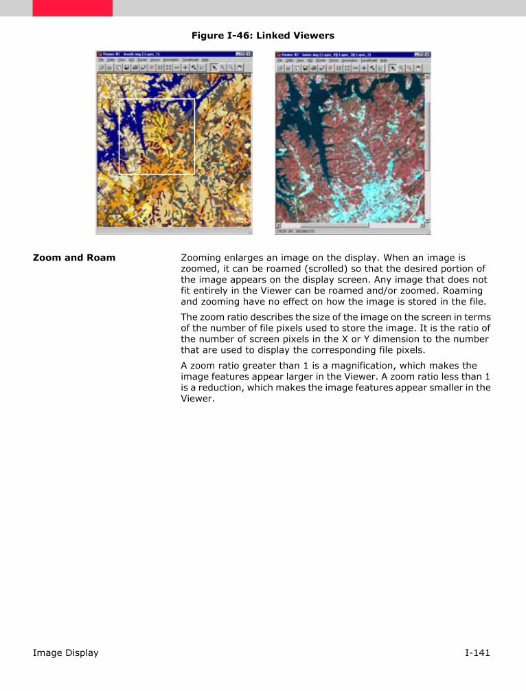
I-141Image Display

Figure I-46: Linked Viewers

Zoom and Roam Zooming enlarges an image on the display. When an image is zoomed, it can be roamed (scrolled) so that the desired portion of the image appears on the display screen. Any image that does not fit entirely in the Viewer can be roamed and/or zoomed. Roaming and zooming have no effect on how the image is stored in the file.

The zoom ratio describes the size of the image on the screen in terms of the number of file pixels used to store the image. It is the ratio of the number of screen pixels in the X or Y dimension to the number that are used to display the corresponding file pixels.

A zoom ratio greater than 1 is a magnification, which makes the image features appear larger in the Viewer. A zoom ratio less than 1 is a reduction, which makes the image features appear smaller in the Viewer.

I-142 Image Display

NOTE: ERDAS IMAGINE allows floating point zoom ratios, so that images can be zoomed at virtually any scale (i.e., continuous fractional zoom). Resampling is necessary whenever an image is displayed with a new pixel grid. The resampling method used when an image is zoomed is the same one used when the image is displayed, as specified in the Open Raster Layer dialog. The default resampling method is Nearest Neighbor.

Zoom the data in the Viewer via the Viewer menu bar, the Viewer tool bar, or the Quick View right-button menu.

Geographic Information To prepare to run many programs, it may be necessary to determine the data file coordinates, map coordinates, or data file values for a particular pixel or a group of pixels. By displaying the image in the Viewer and then selecting the pixel(s) of interest, important information about the pixel(s) can be viewed.

The Quick View right-button menu gives you options to view information about a specific pixel. Use the Raster Attribute Editor to access information about classes in a thematic layer.

See "Geographic Information Systems" on page I-145 for information about attribute data.

Enhancing Continuous Raster Layers

Working with the brightness values in the colormap is useful for image enhancement. Often, a trial and error approach is needed to produce an image that has the right contrast and highlights the right features. By using the tools in the Viewer, it is possible to quickly view the effects of different enhancement techniques, undo enhancements that are not helpful, and then save the best results to disk.

Table I-33: Overview of Zoom Ratio

A zoom ratio of 1 means... each file pixel is displayed with 1 screen pixel in the Viewer.

A zoom ratio of 2 means... each file pixel is displayed with a block of 2 × 2 screen pixels. Effectively, the image is displayed at 200%.

A zoom ratio of 0.5 means... each block of 2 × 2 file pixels is displayed with 1 screen pixel. Effectively, the image is displayed at 50%.

I-143Image Display

Use the Raster options from the Viewer to enhance continuous raster layers.

See "Enhancement" on page II-11 for more information on enhancing continuous raster layers.

Creating New Image Files It is easy to create a new image file (.img) from the layer(s) displayed in the Viewer. The new image file contains three continuous raster layers (RGB), regardless of how many layers are currently displayed. The Image Information utility must be used to create statistics for the new image file before the file is enhanced.

Annotation layers can be converted to raster format, and written to an image file. Or, vector data can be gridded into an image, overwriting the values of the pixels in the image plane, and incorporated into the same band as the image.

Use the Viewer to .img function to create a new image file from the currently displayed raster layers.

I-144 Image Display

I-145Geographic Information Systems

Geographic Information Systems

Introduction The dawning of GIS can legitimately be traced back to the beginning of the human race. The earliest known map dates back to 2500 B.C.E., but there were probably maps before that time. Since then, humans have been continually improving the methods of conveying spatial information. The mid-eighteenth century brought the use of map overlays to show troop movements in the Revolutionary War. This could be considered an early GIS. The first British census in 1825 led to the science of demography, another application for GIS. During the 1800s, many different cartographers and scientists were all discovering the power of overlays to convey multiple levels of information about an area ( Star and Estes, 1990).

Frederick Law Olmstead has long been considered the father of Landscape Architecture for his pioneering work in the early 20th century. Many of the methods Olmstead used in Landscape Architecture also involved the use of hand-drawn overlays. This type of analysis was beginning to be used for a much wider range of applications, such as change detection, urban planning, and resource management ( Rado, 1992).

The first system to be called a GIS was the Canadian Geographic Information System, developed in 1962 by Roger Tomlinson of the Canada Land Inventory. Unlike earlier systems that were developed for a specific application, this system was designed to store digitized map data and land-based attributes in an easily accessible format for all of Canada. This system is still in operation today ( Parent and Church, 1987).

In 1969, Ian McHarg’s influential work, Design with Nature, was published. This work on land suitability/capability analysis (SCA), a system designed to analyze many data layers to produce a plan map, discussed the use of overlays of spatially referenced data layers for resource planning and management ( Star and Estes, 1990).

The era of modern GIS really started in the 1970s, as analysts began to program computers to automate some of the manual processes. Software companies like ESRI and ERDAS developed software packages that could input, display, and manipulate geographic data to create new layers of information. The steady advances in features and power of the hardware over the last ten years—and the decrease in hardware costs—have made GIS technology accessible to a wide range of users. The growth rate of the GIS industry in the last several years has exceeded even the most optimistic projections.

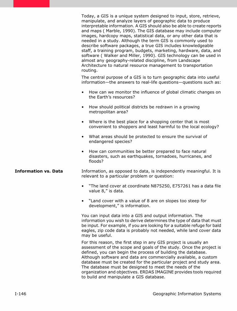
I-146 Geographic Information Systems

Today, a GIS is a unique system designed to input, store, retrieve, manipulate, and analyze layers of geographic data to produce interpretable information. A GIS should also be able to create reports and maps ( Marble, 1990). The GIS database may include computer images, hardcopy maps, statistical data, or any other data that is needed in a study. Although the term GIS is commonly used to describe software packages, a true GIS includes knowledgeable staff, a training program, budgets, marketing, hardware, data, and software ( Walker and Miller, 1990). GIS technology can be used in almost any geography-related discipline, from Landscape Architecture to natural resource management to transportation routing.

The central purpose of a GIS is to turn geographic data into useful information—the answers to real-life questions—questions such as:

• How can we monitor the influence of global climatic changes on the Earth’s resources?

• How should political districts be redrawn in a growing metropolitan area?

• Where is the best place for a shopping center that is most convenient to shoppers and least harmful to the local ecology?

• What areas should be protected to ensure the survival of endangered species?

• How can communities be better prepared to face natural disasters, such as earthquakes, tornadoes, hurricanes, and floods?

Information vs. Data Information, as opposed to data, is independently meaningful. It is relevant to a particular problem or question:

• “The land cover at coordinate N875250, E757261 has a data file value 8,” is data.

• “Land cover with a value of 8 are on slopes too steep for development,” is information.

You can input data into a GIS and output information. The information you wish to derive determines the type of data that must be input. For example, if you are looking for a suitable refuge for bald eagles, zip code data is probably not needed, while land cover data may be useful.

For this reason, the first step in any GIS project is usually an assessment of the scope and goals of the study. Once the project is defined, you can begin the process of building the database. Although software and data are commercially available, a custom database must be created for the particular project and study area. The database must be designed to meet the needs of the organization and objectives. ERDAS IMAGINE provides tools required to build and manipulate a GIS database.

I-147Geographic Information Systems

Successful GIS implementation typically includes two major steps:

• data input

• analysis

Data input involves collecting the necessary data layers into a GIS database. In the analysis phase, these data layers are combined and manipulated in order to create new layers and to extract meaningful information from them. This chapter discusses these steps in detail.

Data Input Acquiring the appropriate data for a project involves creating a database of layers that encompasses the study area. A database created with ERDAS IMAGINE can consist of:

• continuous layers (satellite imagery, aerial photographs, elevation data, etc.)

• thematic layers (land use, vegetation, hydrology, soils, slope, etc.)

• vector layers (streets, utility and communication lines, parcels, etc.)

• statistics (frequency of an occurrence, population demographics, etc.)

• attribute data (characteristics of roads, land, imagery, etc.)

The ERDAS IMAGINE software package employs a hierarchical, object-oriented architecture that utilizes both raster imagery and topological vector data. Raster images are stored in image files, and vector layers are coverages or shapefiles based on the ESRI ArcInfo and ArcView data models. The seamless integration of these two types of data enables you to reap the benefits of both data formats in one system.

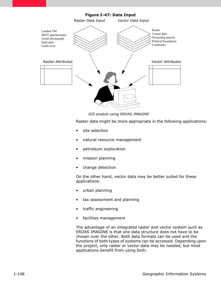
I-148 Geographic Information Systems

Figure I-47: Data Input

Raster data might be more appropriate in the following applications:

• site selection

• natural resource management

• petroleum exploration

• mission planning

• change detection

On the other hand, vector data may be better suited for these applications:

• urban planning

• tax assessment and planning

• traffic engineering

• facilities management

The advantage of an integrated raster and vector system such as ERDAS IMAGINE is that one data structure does not have to be chosen over the other. Both data formats can be used and the functions of both types of systems can be accessed. Depending upon the project, only raster or vector data may be needed, but most applications benefit from using both.

GIS analyst using ERDAS IMAGINE

Landsat TMSPOT panchromaticAerial photographSoils dataLand cover

RoadsCensus dataOwnership parcelsPolitical boundariesLandmarks

Vector Data Input Raster Data Input

Raster Attributes Vector Attributes

I-149Geographic Information Systems

Themes and Layers

A database usually consists of files with data of the same geographical area, with each file containing different types of information. For example, a database for the city recreation department might include files of all the parks in the area. These files might depict park boundaries, county and municipal boundaries, vegetation types, soil types, drainage basins, slope, roads, etc. Each of these files contains different information—each is a different theme. The concept of themes has evolved from early GISs, in which transparent overlays were created for each theme and combined (overlaid) in different ways to derive new information.

A single theme may require more than a simple raster or vector file to fully describe it. In addition to the image, there may be attribute data that describe the information, a color scheme, or meaningful annotation for the image. The full collection of data that describe a certain theme is called a layer.

Depending upon the goals of a project, it may be helpful to combine several themes into one layer. For example, if you want to propose a new park site, you might create one layer that shows roads, land cover, land ownership, slope, etc., and indicate through the use of colors and/or annotation which areas would be best for the new site. This one layer would then include many separate themes. Much of GIS analysis is concerned with combining individual themes into one or more layers that answer the questions driving the analysis. This chapter explores these analysis techniques.

Continuous Layers

Continuous raster layers are quantitative (measuring a characteristic) and have related, continuous values. Continuous raster layers can be multiband (e.g., Landsat TM) or single band (e.g., SPOT panchromatic).

Satellite images, aerial photographs, elevation data, scanned maps, and other continuous raster layers can be incorporated into a database and provide a wealth of information that is not available in thematic layers or vector layers. In fact, these layers often form the foundation of the database. Extremely accurate base maps can be created from rectified satellite images or aerial photographs. Then, all other layers that are added to the database can be registered to this base map.

Once used only for image processing, continuous data are now being incorporated into GIS databases and used in combination with thematic data to influence processing algorithms or as backdrop imagery on which to display the results of analyses. Current satellite data and aerial photographs are also effective in updating outdated vector data. The vectors can be overlaid on the raster backdrop and updated dynamically to reflect new or changed features, such as roads, utility lines, or land use. This chapter explores the many uses of continuous data in a GIS.

I-150 Geographic Information Systems

See "Raster Data" on page I-1 for more information on continuous data.

Thematic Layers Thematic data are typically represented as single layers of information stored as image files and containing discrete classes. Classes are simply categories of pixels which represent the same condition. An example of a thematic layer is a vegetation classification with discrete classes representing coniferous forest, deciduous forest, wetlands, agriculture, urban, etc.

A thematic layer is sometimes called a variable, because it represents one of many characteristics about the study area. Since thematic layers usually have only one band, they are usually displayed in pseudo color mode, where particular colors are often assigned to help visualize the information. For example, blues are usually used for water features, greens for healthy vegetation, etc.

See "Image Display" on page I-117 for information on pseudo color display.

Class Numbering Systems

As opposed to the data file values of continuous raster layers, which are generally multiband and statistically related, the data file values of thematic raster layers can have a nominal, ordinal, interval, or ratio relationship ( Star and Estes, 1990).

• Nominal classes represent categories with no particular order. Usually, these are characteristics that are not associated with quantities (e.g., soil type or political area).

• Ordinal classes are those that have a sequence, such as poor, good, better, and best. An ordinal class numbering system is often created from a nominal system, in which classes have been ranked by some criteria. In the case of the recreation department database used in the previous example, the final layer may rank the proposed park sites according to their overall suitability.

• Interval classes also have a natural sequence, but the distance between each value is meaningful as well. This numbering system might be used for temperature data.

• Ratio classes differ from interval classes only in that ratio classes have a natural zero point, such as rainfall amounts.

I-151Geographic Information Systems

The variable being analyzed, and the way that it contributes to the final product, determines the class numbering system used in the thematic layers. Layers that have one numbering system can easily be recoded to a new system. This is discussed in detail under “Recoding” on page I-161.

Classification

Thematic layers can be generated from remotely sensed data (e.g., Landsat TM, SPOT) by using the ERDAS IMAGINE Image Interpreter, Classification, and Spatial Modeler tools. A frequent and popular application is the creation of land cover classification schemes through the use of both supervised (user-assisted) and unsupervised (automatic) pattern-recognition algorithms contained within ERDAS IMAGINE. The output is a single thematic layer that represents specific classes based on the approach selected.

See "Classification" on page II-99 for more information.

Vector Data Converted to Raster Format

Vector layers can be converted to raster format if the raster format is more appropriate for an application. Typical vector layers, such as communication lines, streams, boundaries, and other linear features, can easily be converted to raster format within ERDAS IMAGINE for further analysis. Spatial Modeler automatically converts vector layers to raster for processing.

Use the Vector Utilities menu from the Vector icon in the ERDAS IMAGINE icon panel to convert vector layers to raster format, or use the vector layers directly in Spatial Modeler.

Other sources of raster data are discussed in "Raster and Vector Data Sources" on page I-49.

Statistics Both continuous and thematic layers include statistical information. Thematic layers contain the following information:

• a histogram of the data values, which is the total number of pixels in each class

• a list of class names that correspond to class values

• a list of class values

• a color table, stored as brightness values in red, green, and blue, which make up the colors of each class when the layer is displayed

I-152 Geographic Information Systems

For thematic data, these statistics are called attributes and may be accompanied by many other types of information, as described in “Attributes” on page I-152.

Use the Image Information option on the Viewer’s tool bar to generate or update statistics for image files.

See "Raster Data" on page I-1 for more information about the statistics stored with continuous layers.

Vector Layers The vector layers used in ERDAS IMAGINE are based on the ArcInfo data model and consist of points, lines, and polygons. These layers are topologically complete, meaning that the spatial relationships between features are maintained. Vector layers can be used to represent transportation routes, utility corridors, communication lines, tax parcels, school zones, voting districts, landmarks, population density, etc. Vector layers can be analyzed independently or in combination with continuous and thematic raster layers.

In ERDAS IMAGINE, vector layers may also be shapefiles based on the ArcView data model.

Vector data can be acquired from several private and governmental agencies. Vector data can also be created in ERDAS IMAGINE by digitizing on the screen, using a digitizing tablet, or converting other data types to vector format.

See "Vector Data" on page I-35 for more information on the characteristics of vector data.

Attributes Text and numerical data that are associated with the classes of a thematic layer or the features in a vector layer are called attributes. This information can take the form of character strings, integer numbers, or floating point numbers. Attributes work much like the data that are handled by database management software. You may define fields, which are categories of information about each class. A record is the set of all attribute data for one class. Each record is like an index card, containing information about one class or feature in a file of many index cards, which contain similar information for the other classes or features.

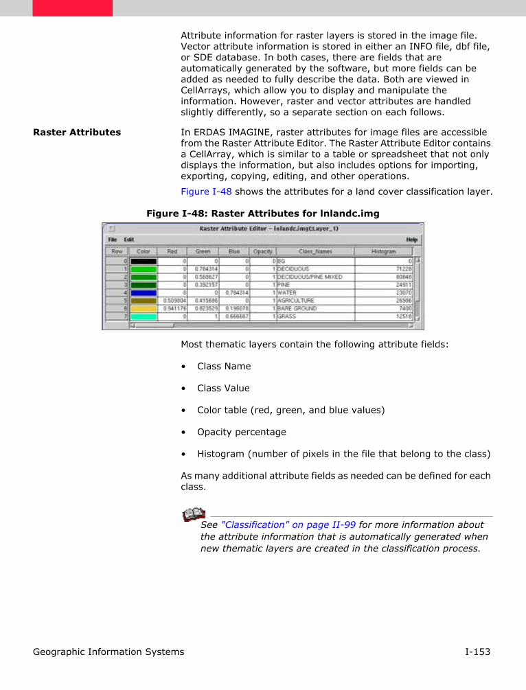
I-153Geographic Information Systems

Attribute information for raster layers is stored in the image file. Vector attribute information is stored in either an INFO file, dbf file, or SDE database. In both cases, there are fields that are automatically generated by the software, but more fields can be added as needed to fully describe the data. Both are viewed in CellArrays, which allow you to display and manipulate the information. However, raster and vector attributes are handled slightly differently, so a separate section on each follows.

Raster Attributes In ERDAS IMAGINE, raster attributes for image files are accessible from the Raster Attribute Editor. The Raster Attribute Editor contains a CellArray, which is similar to a table or spreadsheet that not only displays the information, but also includes options for importing, exporting, copying, editing, and other operations.

Figure I-48 shows the attributes for a land cover classification layer.

Figure I-48: Raster Attributes for lnlandc.img

Most thematic layers contain the following attribute fields:

• Class Name

• Class Value

• Color table (red, green, and blue values)

• Opacity percentage

• Histogram (number of pixels in the file that belong to the class)

As many additional attribute fields as needed can be defined for each class.

See "Classification" on page II-99 for more information about the attribute information that is automatically generated when new thematic layers are created in the classification process.

I-154 Geographic Information Systems

Viewing Raster Attributes

Simply viewing attribute information can be a valuable analysis tool. Depending on the type of information associated with the layers of a database, processing may be further refined by comparing the attributes of several files. When both the raster layer and its associated attribute information are displayed, you can select features in one using the other. For example, to locate the class name associated with a particular area in a displayed image, simply click in that area with the mouse and the associated row is highlighted in the Raster Attribute Editor.

Attribute information is accessible in several places throughout ERDAS IMAGINE. In some cases it is read-only and in other cases it is a fully functioning editor, allowing the information to be modified.

Manipulating Raster Attributes

The applications for manipulating attributes are as varied as the applications for GIS. The attribute information in a database depends on the goals of the project. Some of the attribute editing capabilities in ERDAS IMAGINE include:

• import/export ASCII information to and from other software packages, such as spreadsheets and word processors

• cut, copy, and paste individual cells, rows, or columns to and from the same Raster Attribute Editor or among several Raster Attribute Editors

• generate reports that include all or a subset of the information in the Raster Attribute Editor

• use formulas to populate cells

• directly edit cells by entering in new information

The Raster Attribute Editor in ERDAS IMAGINE also includes a color cell column, so that class (object) colors can be viewed or changed. In addition to direct manipulation, attributes can be changed by other programs. For example, some of the Image Interpreter functions calculate statistics that are automatically added to the Raster Attribute Editor. Models that read and/or modify attribute information can also be written.

See "Enhancement" for more information on the Image Interpreter. There is more information on GIS modeling in “Graphical Modeling” on page I-166.

Vector Attributes Vector attributes are stored in the Vector Attributes CellArrays. You can simply view attributes or use them to:

• select features in a vector layer for further processing

I-155Geographic Information Systems

• determine how vectors are symbolized

• label features

Figure I-49 shows the attributes for a roads layer.

Figure I-49: Vector Attributes CellArray

See "Vector Data" on page I-35 for more information about vector attributes.

Analysis

ERDAS IMAGINE Analysis Tools

In ERDAS IMAGINE, GIS analysis functions and algorithms are accessible through three main tools:

• script models created with SML

• graphical models created with Model Maker

• prepackaged functions in Image Interpreter

Spatial Modeler Language

SML is the basis for all ERDAS IMAGINE GIS functions. It is a modeling language that enables you to create script (text) models for a variety of applications. Models may be used to create custom algorithms that best suit your data and objectives.

I-156 Geographic Information Systems

Model Maker

Model Maker is essentially SML linked to a graphical interface. This enables you to create graphical models using a palette of easy-to-use tools. Graphical models can be run, edited, saved in libraries, or converted to script form and edited further, using SML.

NOTE: References to the Spatial Modeler in this chapter mean that the named procedure can be accomplished using both Model Maker and SML.

Image Interpreter

The Image Interpreter houses a set of common functions that were all created using either Model Maker or SML. They have been given a dialog interface to match the other processes in ERDAS IMAGINE. In most cases, these processes can be run from a single dialog. However, the actual models are also provided with the software to enable customized processing.

Many of the functions described in the following sections can be accomplished using any of these tools. Model Maker is also easy to use and utilizes many of the same steps that would be performed when drawing a flow chart of an analysis. SML is intended for more advanced analyses, and has been designed using natural language commands and simple syntax rules. Some applications may require a combination of these tools.

Customizing ERDAS IMAGINE Tools

ERDAS Macro Language (EML) enables you to create and add new and/or customized dialogs. If new capabilities are needed, they can be created with the IMAGINE Developers’ Toolkit™. Using these tools, a GIS that is completely customized to a specific application and its preferences can be created.

See the ERDAS IMAGINE On-Line Help for more information about EML and the IMAGINE Developers’ Toolkit.

Analysis Procedures Once the database (layers and attribute data) is assembled, the layers can be analyzed and new information extracted. Some information can be extracted simply by looking at the layers and visually comparing them to other layers. However, new information can be retrieved by combining and comparing layers using the following procedures:

• Proximity analysis—the process of categorizing and evaluating pixels based on their distances from other pixels in a specified class or classes.

• Contiguity analysis—enables you to identify regions of pixels in the same class and to filter out small regions.

I-157Geographic Information Systems

• Neighborhood analysis —any image processing technique that takes surrounding pixels into consideration, such as convolution filtering and scanning. This is similar to the convolution filtering performed on continuous data. Several types of analyses can be performed, such as boundary, density, mean, sum, etc.

• Recoding—enables you to assign new class values to all or a subset of the classes in a layer.

• Overlaying—creates a new file with either the maximum or minimum value of the input layers.

• Indexing—adds the values of the input layers.

• Matrix analysis—outputs the coincidence values of the input layers.

• Graphical modeling—enables you to combine data layers in an unlimited number of ways. For example, an output layer created from modeling can represent the desired combination of themes from many input layers.

• Script modeling—offers all of the capabilities of graphical modeling with the ability to perform more complex functions, such as conditional looping.

Using an Area of Interest

Any of these functions can be performed on a single layer or multiple layers. You can also select a particular AOI that is defined in a separate file (AOI layer, thematic raster layer, or vector layer) or an AOI that is selected immediately preceding the operation by entering specific coordinates or by selecting the area in a Viewer.

Proximity Analysis

Many applications require some measurement of distance or proximity. For example, a real estate developer would be concerned with the distance between a potential site for a shopping center and an interchange to a major highway.

Proximity analysis determines which pixels of a layer are located at specified distances from pixels in a certain class or classes. A new thematic layer (image file) is created, which is categorized by the distance of each pixel from specified classes of the input layer. This new file then becomes a new layer of the database and provides a buffer zone around the specified class(es). In further analysis, it may be beneficial to weight other factors, based on whether they fall inside or outside the buffer zone.

Figure I-50 shows a layer containing lakes and streams and the resulting layer after a proximity analysis is run to create a buffer zone around all of the water features.

I-158 Geographic Information Systems

Use the Search (GIS Analysis) function in Image Interpreter or Spatial Modeler to perform a proximity analysis.

Figure I-50: Proximity Analysis

Contiguity Analysis

Contiguity analysis is concerned with the ways in which pixels of a class are grouped together. Groups of contiguous pixels in the same class, called raster regions, or clumps, can be identified by their sizes and manipulated. One application of this tool would be an analysis for locating helicopter landing zones that require at least 250 contiguous pixels at 10-meter resolution.

Contiguity analysis can be used to: 1) divide a large class into separate raster regions, or 2) eliminate raster regions that are too small to be considered for an application.

Filtering Clumps

In cases where very small clumps are not useful, they can be filtered out according to their sizes. This is sometimes referred to as eliminating the salt and pepper effects, or sieving. In Figure I-51, all of the small clumps in the original (clumped) layer are eliminated.

Figure I-51: Contiguity Analysis

Original layer After proximity analysis performed

Buffer

Lake

Streams

zones

Clumped layer Sieved layer

I-159Geographic Information Systems

Use the Clump and Sieve (GIS Analysis) function in Image Interpreter or Spatial Modeler to perform contiguity analysis.

Neighborhood Analysis

With a process similar to the convolution filtering of continuous raster layers, thematic raster layers can also be filtered. The GIS filtering process is sometimes referred to as scanning, but is not to be confused with data capture via a digital camera. Neighborhood analysis is based on local or neighborhood characteristics of the data ( Star and Estes, 1990).

Every pixel is analyzed spatially, according to the pixels that surround it. The number and the location of the surrounding pixels is determined by a scanning window, which is defined by you. These operations are known as focal operations. The scanning window can be of any size in SML. In Model Maker, it has the following constraints:

• circular, with a maximum diameter of 512 pixels

• doughnut-shaped, with a maximum outer radius of 256

• rectangular, up to 512 × 512 pixels, with the option to mask-out certain pixels

Use the Neighborhood (GIS Analysis) function in Image Interpreter or Spatial Modeler to perform neighborhood analysis. The scanning window used in Image Interpreter can be 3 × 3, 5 × 5, or 7 × 7. The scanning window in Model Maker is defined by you and can be up to 512 × 512. The scanning window in SML can be of any size.

Defining Scan Area

You may define the area of the file to be scanned. The scanning window moves only through this area as the analysis is performed. Define the area in one or all of the following ways:

• Specify a rectangular portion of the file to scan. The output layer contains only the specified area.

• Specify an area that is defined by an existing AOI layer, an annotation overlay, or a vector layer. The area(s) within the polygon are scanned, and the other areas remain the same. The output layer is the same size as the input layer or the selected rectangular portion.

I-160 Geographic Information Systems

• Specify a class or classes in another thematic layer to be used as a mask. The pixels in the scanned layer that correspond to the pixels of the selected class or classes in the mask layer are scanned, while the other pixels remain the same.

Figure I-52: Using a Mask

In Figure I-52, class 2 in the mask layer was selected for the mask. Only the corresponding (shaded) pixels in the target layer are scanned—the other values remain unchanged.

Neighborhood analysis creates a new thematic layer. There are several types of analysis that can be performed upon each window of pixels, as described below:

• Boundary—detects boundaries between classes. The output layer contains only boundary pixels. This is useful for creating boundary or edge lines from classes, such as a land/water interface.

• Density—outputs the number of pixels that have the same class value as the center (analyzed) pixel. This is also a measure of homogeneity (sameness), based upon the analyzed pixel. This is often useful in assessing vegetation crown closure.

• Diversity—outputs the number of class values that are present within the window. Diversity is also a measure of heterogeneity (difference).

• Majority—outputs the class value that represents the majority of the class values in the window. The value is defined by you. This option operates like a low-frequency filter to clean up a salt and pepper layer.

• Maximum—outputs the greatest class value within the window. This can be used to emphasize classes with the higher class values or to eliminate linear features or boundaries.

• Mean—averages the class values. If class values represent quantitative data, then this option can work like a convolution filter. This is mostly used on ordinal or interval data.

88222288222

26666226668

88888668334

45533344544

44454444555

55555

mask layer target layer

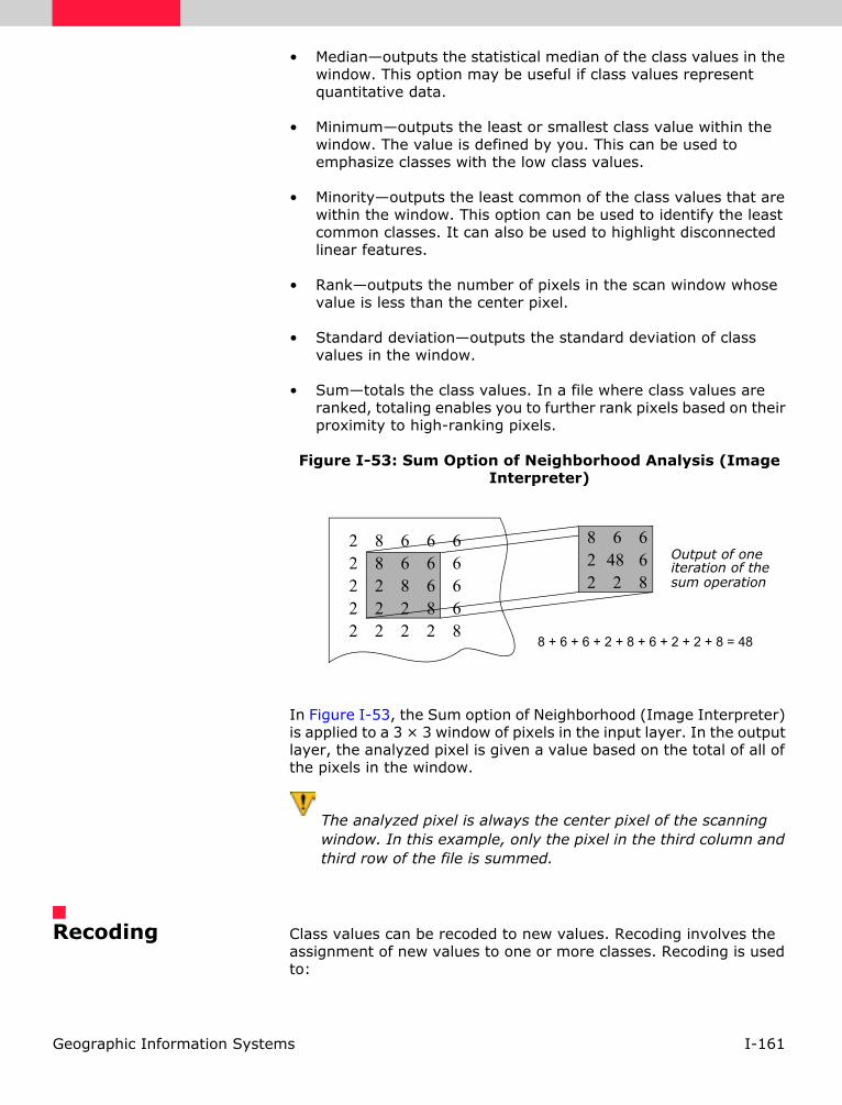
I-161Geographic Information Systems

• Median—outputs the statistical median of the class values in the window. This option may be useful if class values represent quantitative data.

• Minimum—outputs the least or smallest class value within the window. The value is defined by you. This can be used to emphasize classes with the low class values.

• Minority—outputs the least common of the class values that are within the window. This option can be used to identify the least common classes. It can also be used to highlight disconnected linear features.

• Rank—outputs the number of pixels in the scan window whose value is less than the center pixel.

• Standard deviation—outputs the standard deviation of class values in the window.

• Sum—totals the class values. In a file where class values are ranked, totaling enables you to further rank pixels based on their proximity to high-ranking pixels.

Figure I-53: Sum Option of Neighborhood Analysis (Image Interpreter)

In Figure I-53, the Sum option of Neighborhood (Image Interpreter) is applied to a 3 × 3 window of pixels in the input layer. In the output layer, the analyzed pixel is given a value based on the total of all of the pixels in the window.

The analyzed pixel is always the center pixel of the scanning window. In this example, only the pixel in the third column and third row of the file is summed.

Recoding Class values can be recoded to new values. Recoding involves the assignment of new values to one or more classes. Recoding is used to:

22222

88222

66822

66682

66668

822

6482

668

Output of oneiteration of thesum operation

8 + 6 + 6 + 2 + 8 + 6 + 2 + 2 + 8 = 48

I-162 Geographic Information Systems

• reduce the number of classes

• combine classes

• assign different class values to existing classes

When an ordinal, ratio, or interval class numbering system is used, recoding can be used to assign classes to appropriate values. Recoding is often performed to make later steps easier. For example, in creating a model that outputs good, better, and best areas, it may be beneficial to recode the input layers so all of the best classes have the highest class values.

In the following example (Table I-34, “Example of a Recoded Land Cover Layer,” on page I-162), a land cover layer is recoded so that the most environmentally sensitive areas (Riparian and Wetlands) have higher class values.

Use the Recode (GIS Analysis) function in Image Interpreter or Spatial Modeler to recode layers.

Overlaying Thematic data layers can be overlaid to create a composite layer. The output layer contains either the minimum or the maximum class values of the input layers. For example, if an area was in class 5 in one layer, and in class 3 in another, and the maximum class value dominated, then the same area would be coded to class 5 in the output layer, as shown in Figure I-54.

Table I-34: Example of a Recoded Land Cover Layer

Value New Value Class Name

0 0 Background

1 4 Riparian

2 1 Grassland and Scrub

3 1 Chaparral

4 4 Wetlands

5 1 Emergent Vegetation

6 1 Water

I-163Geographic Information Systems

Figure I-54: Overlay

The application example in Figure I-54 shows the result of combining two layers—slope and land use. The slope layer is first recoded to combine all steep slopes into one value. When overlaid with the land use layer, the highest data file values (the steep slopes) dominate in the output layer.

Use the Overlay (GIS Analysis) function in Image Interpreter or Spatial Modeler to overlay layers.

Indexing Thematic layers can be indexed (added) to create a composite layer. The output layer contains the sums of the input layer values. For example, the intersection of class 3 in one layer and class 5 in another would result in class 8 in the output layer, as shown in Figure I-55.

68

92

16

13

5

22

34

12

25

3

99

94

19

25

3

99

90

09

00

0

Recode

Overlay

Original Slope1-5 = flat slopes6-9 = steep slopes

Recoded Slope0 = flat slopes9 = steep slopes

Land Use1 = commercial2 = residential3 = forest4 = industrial5 = wetlands

Overlay Composite1 = commercial2 = residential3 = forest4 = industrial5 = wetlands9 = steep slopes

(Land Use masked)

53

Basic Overlay Application Example

I-164 Geographic Information Systems

Figure I-55: Indexing

The application example in Figure I-55 shows the result of indexing. In this example, you want to develop a new subdivision, and the most likely sites are where there is the best combination (highest value) of good soils, good slope, and good access. Because good slope is a more critical factor to you than good soils or good access, a weighting factor is applied to the slope layer. A weighting factor has the effect of multiplying all input values by some constant. In this example, slope is given a weight of 2.

Use the Index (GIS Analysis) function in the Image Interpreter or Spatial Modeler to index layers.

99

59

91

19

5

95

19

95

99

9

3624

1636

368

2836

16

1810

1018

182

1818

2

Soils9 = good5 = fair

Slope9 = good5 = fair

Access9 = good5 = fair1 = poor

1 = poor

1 = poor

Output values calculated

WeightingImportance×1×1×1

WeightingImportance×2×2×2

WeightingImportance×1×1×1

+

+

=

3 58

Basic Index Application Example

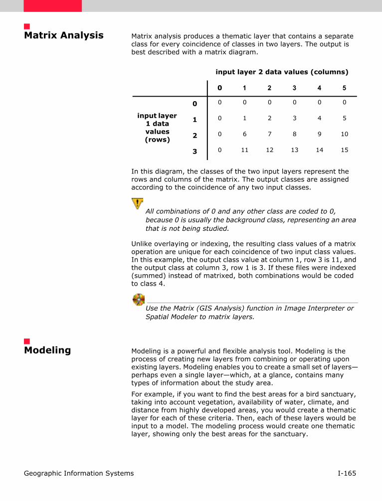
I-165Geographic Information Systems

Matrix Analysis Matrix analysis produces a thematic layer that contains a separate class for every coincidence of classes in two layers. The output is best described with a matrix diagram.

In this diagram, the classes of the two input layers represent the rows and columns of the matrix. The output classes are assigned according to the coincidence of any two input classes.

All combinations of 0 and any other class are coded to 0, because 0 is usually the background class, representing an area that is not being studied.

Unlike overlaying or indexing, the resulting class values of a matrix operation are unique for each coincidence of two input class values. In this example, the output class value at column 1, row 3 is 11, and the output class at column 3, row 1 is 3. If these files were indexed (summed) instead of matrixed, both combinations would be coded to class 4.

Use the Matrix (GIS Analysis) function in Image Interpreter or Spatial Modeler to matrix layers.

Modeling Modeling is a powerful and flexible analysis tool. Modeling is the process of creating new layers from combining or operating upon existing layers. Modeling enables you to create a small set of layers—perhaps even a single layer—which, at a glance, contains many types of information about the study area.

For example, if you want to find the best areas for a bird sanctuary, taking into account vegetation, availability of water, climate, and distance from highly developed areas, you would create a thematic layer for each of these criteria. Then, each of these layers would be input to a model. The modeling process would create one thematic layer, showing only the best areas for the sanctuary.

input layer 2 data values (columns)

0 1 2 3 4 5

input layer 1 data values (rows)

0 0 0 0 0 0 0

1 0 1 2 3 4 5

2 0 6 7 8 9 10

3 0 11 12 13 14 15

I-166 Geographic Information Systems

The set of procedures that define the criteria is called a model. In ERDAS IMAGINE, models can be created graphically and resemble a flow chart of steps, or they can be created using a script language. Although these two types of models look different, they are essentially the same—input files are defined, functions and/or operators are specified, and outputs are defined. The model is run and a new output layer(s) is created. Models can utilize analysis functions that have been previously defined, or new functions can be created by you.

Use the Model Maker function in Spatial Modeler to create graphical models and SML to create script models.

Data Layers

In modeling, the concept of layers is especially important. Before computers were used for modeling, the most widely used approach was to overlay registered maps on paper or transparencies, with each map corresponding to a separate theme. Today, digital files replace these hardcopy layers and allow much more flexibility for recoloring, recoding, and reproducing geographical information ( Steinitz et al, 1976).

In a model, the corresponding pixels at the same coordinates in all input layers are addressed as if they were physically overlaid like hardcopy maps.

Graphical Modeling

Graphical modeling enables you to draw models using a palette of tools that defines inputs, functions, and outputs. This type of modeling is very similar to drawing flowcharts, in that you identify a logical flow of steps needed to perform the desired action. Through the extensive functions and operators available in the ERDAS IMAGINE graphical modeling program, you can analyze many layers of data in very few steps without creating intermediate files that occupy extra disk space. Modeling is performed using a graphical editor that eliminates the need to learn a programming language. Complex models can be developed easily and then quickly edited and re-run on another data set.

Use the Model Maker function in Spatial Modeler to create graphical models.

Image Processing and GIS

In ERDAS IMAGINE, the traditional GIS functions (e.g., neighborhood analysis, proximity analysis, recode, overlay, index, etc.) can be performed in models, as well as image processing functions. Both thematic and continuous layers can be input into models that accomplish many objectives at once.

I-167Geographic Information Systems

For example, suppose there is a need to assess the environmental sensitivity of an area for development. An output layer can be created that ranks most to least sensitive regions based on several factors, such as slope, land cover, and floodplain. To visualize the location of these areas, the output thematic layer can be overlaid onto a high resolution, continuous raster layer (e.g., SPOT panchromatic) that has had a convolution filter applied. All of this can be accomplished in a single model (as shown in Figure I-56).

Figure I-56: Graphical Model for Sensitivity Analysis

See the ERDAS IMAGINE Tour Guides manual for step-by-step instructions on creating the environmental sensitivity model in Figure I-56. Descriptions of all of the graphical models delivered with ERDAS IMAGINE are available in the On-Line Help.

Model Structure

A model created with Model Maker is essentially a flow chart that defines:

• the input image(s), vector(s), matrix(ces), table(s), and scalar(s) to be analyzed

I-168 Geographic Information Systems

• calculations, functions, or operations to be performed on the input data

• the output image(s), matrix(ces), table(s), and scalars to be created

The graphical models created in Model Maker all have the same basic structure: input, function, output. The number of inputs, functions, and outputs can vary, but the overall form remains constant. All components must be connected to one another before the model can be executed. The model on the left in Figure I-57 is the most basic form. The model on the right is more complex, but it retains the same input/function/output flow.

Figure I-57: Graphical Model Structure

Graphical models are stored in ASCII files with the .gmd extension. There are several sample graphical models delivered with ERDAS IMAGINE that can be used as is or edited for more customized processing.

See the On-Line Help for instructions on editing existing models.

Input

Input

Function Output

Basic Model

Input

Function

Output

FunctionInput

Output

Complex Model

I-169Geographic Information Systems

Model Maker Functions The functions available in Model Maker are divided into the following categories:

Table I-35: Model Maker Functions

Category Description

Analysis Includes convolution filtering, histogram matching, contrast stretch, principal components, and more.

Arithmetic Perform basic arithmetic functions including addition, subtraction, multiplication, division, factorial, and modulus.

Bitwise Use bitwise and, or, exclusive or, and not.

Boolean Perform logical functions including and, or, and not.

Color Manipulate colors to and from RGB (red, green, blue) and IHS (intensity, hue, saturation).

Conditional Run logical tests using conditional statements and either...if...or...otherwise.

Data Generation Create raster layers from map coordinates, column numbers, or row numbers. Create a matrix or table from a list of scalars.

Descriptor Read attribute information and map a raster through an attribute column.

Distance Perform distance functions, including proximity analysis.

Exponential Use exponential operators, including natural and common logarithmic, power, and square root.

Focal (Scan) Perform neighborhood analysis functions, including boundary, density, diversity, majority, mean, minority, rank, standard deviation, sum, and others.

Focal Use Opts Constraints on which pixel values to include in calculations for the Focal (Scan) function.

Focal Apply Opts Constraints on which pixel values to apply the results of calculations for the Focal (Scan) function.

Global Analyze an entire layer and output one value, such as diversity, maximum, mean, minimum, standard deviation, sum, and more.

Matrix Multiply, divide, and transpose matrices, as well as convert a matrix to a table and vice versa.

Other Includes over 20 miscellaneous functions for data type conversion, various tests, and other utilities.

Relational Includes equality, inequality, greater than, less than, greater than or equal, less than or equal, and others.

Size Measure cell X and Y size, layer width and height, number of rows and columns, etc.

Stack Statistics Perform operations over a stack of layers including diversity, majority, max, mean, median, min, minority, standard deviation, and sum.

Statistical Includes density, diversity, majority, mean, rank, standard deviation, and more.

String Manipulate character strings.

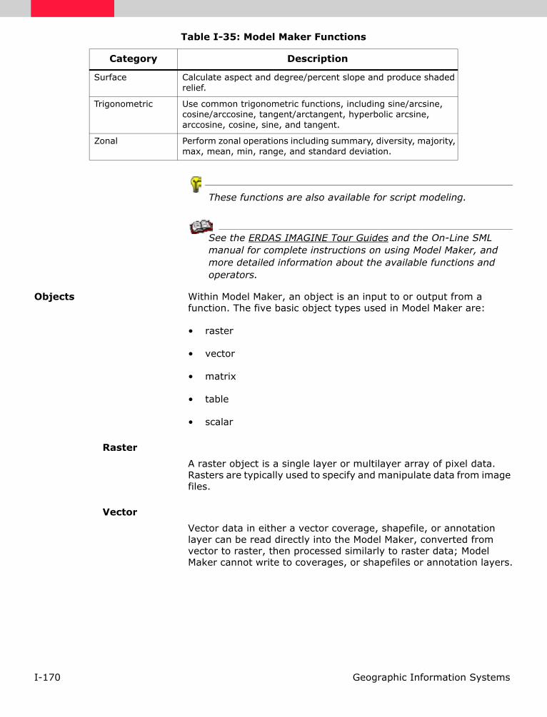
I-170 Geographic Information Systems

These functions are also available for script modeling.

See the ERDAS IMAGINE Tour Guides and the On-Line SML manual for complete instructions on using Model Maker, and more detailed information about the available functions and operators.

Objects Within Model Maker, an object is an input to or output from a function. The five basic object types used in Model Maker are:

• raster

• vector

• matrix

• table

• scalar

Raster

A raster object is a single layer or multilayer array of pixel data. Rasters are typically used to specify and manipulate data from image files.

Vector

Vector data in either a vector coverage, shapefile, or annotation layer can be read directly into the Model Maker, converted from vector to raster, then processed similarly to raster data; Model Maker cannot write to coverages, or shapefiles or annotation layers.

Surface Calculate aspect and degree/percent slope and produce shaded relief.

Trigonometric Use common trigonometric functions, including sine/arcsine, cosine/arccosine, tangent/arctangent, hyperbolic arcsine, arccosine, cosine, sine, and tangent.

Zonal Perform zonal operations including summary, diversity, majority, max, mean, min, range, and standard deviation.

Table I-35: Model Maker Functions

Category Description

I-171Geographic Information Systems

Matrix

A matrix object is a set of numbers arranged in a two-dimensional array. A matrix has a fixed number of rows and columns. Matrices may be used to store convolution kernels or the neighborhood definition used in neighborhood functions. They can also be used to store covariance matrices, eigenvector matrices, or matrices of linear combination coefficients.

Table

A table object is a series of numeric values, colors, or character strings. A table has one column and a fixed number of rows. Tables are typically used to store columns from the Raster Attribute Editor or a list of values that pertains to the individual layers of a set of layers. For example, a table with four rows could be used to store the maximum value from each layer of a four layer image file. A table may consist of up to 32,767 rows. Information in the table can be attributes, calculated (e.g., histograms), or defined by you.

Scalar

A scalar object is a single numeric value, color, or character string. Scalars are often used as weighting factors.

The graphics used in Model Maker to represent each of these objects are shown in Figure I-58.

Figure I-58: Modeling Objects

Data Types The five object types described above may be any of the following data types:

• Binary—either 0 (false) or 1 (true)

• Integer—integer values from -2,147,483,648 to 2,147,483,648 (signed 32-bit integer)

• Float—floating point data (double precision)

• String—a character string (for table objects only)

Raster

Matrix Scalar

Table

+

+

Vector

I-172 Geographic Information Systems

Input and output data types do not have to be the same. Using SML, you can change the data type of input files before they are processed.

Output Parameters Since it is possible to have several inputs in one model, you can optionally define the working window and the pixel cell size of the output data along with the output map projection.

Working Window

Raster layers of differing areas can be input into one model. However, the image area, or working window, must be specified in order to use it in the model calculations. Either of the following options can be selected:

• Union—the model operates on the union of all input rasters. (This is the default.)

• Intersection—the model uses only the area of the rasters that is common to all input rasters.

Pixel Cell Size

Input rasters may also be of differing resolution (pixel size), so you must select the output cell size as either:

• Minimum—the minimum cell size of the input layers is used (this is the default setting).

• Maximum—the maximum cell size of the input layers is used.

• Other—specify a new cell size.

Map Projection

The output map projection defaults to be the same as the first input, or projection may be selected to be the same as a chosen input. The output projection may also be selected from a projection library.

Using Attributes in Models

With the criteria function in Model Maker, attribute data can be used to determine output values. The criteria function simplifies the process of creating a conditional statement. The criteria function can be used to build a table of conditions that must be satisfied to output a particular row value for an attribute (or cell value) associated with the selected raster.

The inputs to a criteria function are rasters or vectors. The columns of the criteria table represent either attributes associated with a raster layer or the layer itself, if the cell values are of direct interest. Criteria which must be met for each output column are entered in a cell in that column (e.g., >5). Multiple sets of criteria may be entered in multiple rows. The output raster contains the first row number of a set of criteria that were met for a raster cell.

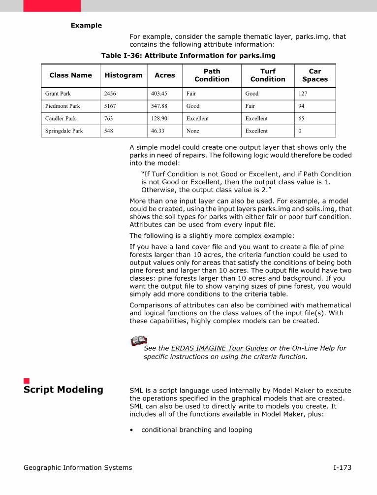
I-173Geographic Information Systems

Example

For example, consider the sample thematic layer, parks.img, that contains the following attribute information:

A simple model could create one output layer that shows only the parks in need of repairs. The following logic would therefore be coded into the model:

“If Turf Condition is not Good or Excellent, and if Path Condition is not Good or Excellent, then the output class value is 1. Otherwise, the output class value is 2.”

More than one input layer can also be used. For example, a model could be created, using the input layers parks.img and soils.img, that shows the soil types for parks with either fair or poor turf condition. Attributes can be used from every input file.

The following is a slightly more complex example:

If you have a land cover file and you want to create a file of pine forests larger than 10 acres, the criteria function could be used to output values only for areas that satisfy the conditions of being both pine forest and larger than 10 acres. The output file would have two classes: pine forests larger than 10 acres and background. If you want the output file to show varying sizes of pine forest, you would simply add more conditions to the criteria table.

Comparisons of attributes can also be combined with mathematical and logical functions on the class values of the input file(s). With these capabilities, highly complex models can be created.

See the ERDAS IMAGINE Tour Guides or the On-Line Help for specific instructions on using the criteria function.

Script Modeling SML is a script language used internally by Model Maker to execute the operations specified in the graphical models that are created. SML can also be used to directly write to models you create. It includes all of the functions available in Model Maker, plus:

• conditional branching and looping

Table I-36: Attribute Information for parks.img

Class Name Histogram Acres Path Condition

Turf Condition

Car Spaces

Grant Park 2456 403.45 Fair Good 127

Piedmont Park 5167 547.88 Good Fair 94

Candler Park 763 128.90 Excellent Excellent 65

Springdale Park 548 46.33 None Excellent 0

I-174 Geographic Information Systems

• the ability to use complex data types

Graphical models created with Model Maker can be output to a script file (text only) in SML. These scripts can then be edited with a text editor using SML syntax and rerun or saved in a library. Script models can also be written from scratch in the text editor. They are stored in ASCII .mdl files.

The Text Editor is available from the Tools menu located on the ERDAS IMAGINE menu bar and from the Model Librarian (Spatial Modeler).

In Figure I-59, both the graphical and script models are shown for a tasseled cap transformation. Notice how even the annotation on the graphical model is included in the automatically generated script model. Generating script models from graphical models may aid in learning SML.

I-175Geographic Information Systems

Figure I-59: Graphical and Script Models For Tasseled Cap Transformation

Convert graphical models to scripts using Model Maker. Open existing script models from the Model Librarian (Spatial Modeler).

Graphical Model

Script Model

Tasseled Cap Transformation

Models

# TM Tasseled Cap Transformation# of Lake Lanier, Georgia## declarations#INTEGER RASTER n1_tm_lanier FILE OLD NEAREST NEIGHBOR "/usr/imagine/examples/tm_lanier.img";FLOAT MATRIX n2_Custom_Matrix;FLOAT RASTER n4_lntassel FILE NEW ATHEMATIC FLOAT SINGLE "/usr/imagine/examples/lntassel.img";## set cell size for the model#SET CELLSIZE MIN;## set window for the model#SET WINDOW UNION;## load matrix n2_Custom_Matrix#n2_Custom_Matrix = MATRIX(3, 7:0.331830, 0.331210, 0.551770, 0.425140, 0.480870, 0.000000, 0.252520, -0.247170, -0.162630, -0.406390, 0.854680, 0.054930, 0.000000, -0.117490, 0.139290, 0.224900, 0.403590, 0.251780, -0.701330, 0.000000, -0.457320);## function definitions#n4_lntassel = LINEARCOMB ( $n1_tm_lanier , $n2_Custom_Matrix ) ;QUIT;

I-176 Geographic Information Systems

Statements A script model consists primarily of one or more statements. Each statement falls into one of the following categories:

• Declaration—defines objects to be manipulated within the model

• Assignment—assigns a value to an object

• Show and View—enables you to see and interpret results from the model

• Set—defines the scope of the model or establishes default values used by the Modeler

• Macro Definition—defines substitution text associated with a macro name

• Quit—ends execution of the model

SML also includes flow control structures so that you can utilize conditional branching and looping in the models and statement block structures, which cause a set of statements to be executed as a group.

Declaration Example

In the script model in Figure I-59, the following lines form the declaration portion of the model:

INTEGER RASTER n1_tm_lanier FILE OLD NEAREST NEIGHBOR "/usr/imagine/examples/tm_lanier.img";

FLOAT MATRIX n2_Custom_Matrix;

FLOAT RASTER n4_lntassel FILE NEW ATHEMATIC FLOAT SINGLE "/usr/imagine/examples/lntassel.img";

Set Example

The following set statements are used:

SET CELLSIZE MIN;

SET WINDOW UNION;

Assignment Example

The following assignment statements are used:

n2_Custom_Matrix = MATRIX(3, 7:

0.331830, 0.331210, 0.551770, 0.425140, 0.480870, 0.000000, 0.252520,

-0.247170, -0.162630, -0.406390, 0.854680, 0.054930, 0.000000, -0.117490,

0.139290, 0.224900, 0.403590, 0.251780, -0.701330, 0.000000, -0.457320);

n4_lntassel = LINEARCOMB ( $n1_tm_lanier , $n2_Custom_Matrix ) ;

I-177Geographic Information Systems

Data Types In addition to the data types utilized by Graphical Modeling, script model objects can store data in the following data types:

• Complex—complex data (double precision)

• Color—three floating point numbers in the range of 0.0 to 1.0, representing intensity of red, green, and blue

Variables Variables are objects in the Modeler that have been associated with names using Declaration Statements. The declaration statement defines the data type and object type of the variable. The declaration may also associate a raster variable with certain layers of an image file or a table variable with an attribute table. Assignment Statements are used to set or change the value of a variable.

For script model syntax rules, descriptions of all available functions and operators, and sample models, see the On-Line SML manual.

Vector Analysis Most of the operations discussed in the previous pages of this chapter focus on raster data. However, in a complete GIS database, both raster and vector layers are present. One of the most common applications involving the combination of raster and vector data is the updating of vector layers using current raster imagery as a backdrop for vector editing. For example, if a vector database is more than one or two years old, then there are probably errors due to changes in the area (new roads, moved roads, new development, etc.). When displaying existing vector layers over a raster layer, you can dynamically update the vector layer by digitizing new or changed features on the screen.

Vector layers can also be used to indicate an AOI for further processing. Assume you want to run a site suitability model on only areas designated for commercial development in the zoning ordinances. By selecting these zones in a vector polygon layer, you could restrict the model to only those areas in the raster input files.

Vector layers can also be used as inputs to models. Updated or new attributes may also be written to vector layers in models.

Editing Vector Layers Editable features are polygons (as lines), lines, label points, and nodes. There can be multiple features selected with a mixture of any and all feature types. Editing operations and commands can be performed on multiple or single selections. In addition to the basic editing operations (e.g., cut, paste, copy, delete), you can also perform the following operations on the line features in multiple or single selections:

• spline—smooths or generalizes all currently selected lines using a specified grain tolerance

I-178 Geographic Information Systems

• generalize—weeds vertices from selected lines using a specified tolerance

• split/unsplit—makes two lines from one by adding a node or joins two lines by removing a node

• densify—adds vertices to selected lines at a tolerance you specify

• reshape (for single lines only)—enables you to move the vertices of a line

Reshaping (adding, deleting, or moving a vertex or node) can be done on a single selected line. Table I-37, “General Editing Operations and Supporting Feature Types” details general editing operations and the feature types that support each of those operations.

The Undo utility may be applied to any edits. The software stores all edits in sequential order, so that continually pressing Undo reverses the editing.

For more information on vectors, see "Raster and Vector Data Sources" on page I-49.

Constructing Topology

Either the Build or Clean option can be used to construct topology. To create spatial relationships between features in a vector layer, it is necessary to create topology. After a vector layer is edited, the topology must be constructed to maintain the topological relationships between features. When topology is constructed, each feature is assigned an internal number. These numbers are then used to determine line connectivity and polygon contiguity. Once calculated, these values are recorded and stored in that layer’s associated attribute table.

You must also reconstruct the topology of vector layers imported into ERDAS IMAGINE.

Table I-37: General Editing Operations and Supporting Feature Types

Add Delete Move Reshape

Points yes yes yes no

Lines yes yes yes yes

Polygons yes yes yes no

Nodes yes yes yes no

I-179Geographic Information Systems

When topology is constructed, feature attribute tables are created with several automatically created fields. Different fields are stored for the different types of layers. The automatically generated fields for a line layer are:

• FNODE#—the internal node number for the beginning of a line (from-node)

• TNODE#—the internal number for the end of a line (to-node)

• LPOLY#—the internal number for the polygon to the left of the line (zero for layers containing only lines and no polygons)

• RPOLY#—the internal number for the polygon to the right of the line (zero for layers containing only lines and no polygons)

• LENGTH—length of each line, measured in layer units

• Cover#—internal line number (values assigned by ERDAS IMAGINE)

• Cover-ID—user-ID (values modified by you)

The automatically generated fields for a point or polygon layer are:

• AREA—area of each polygon, measured in layer units (zero for layers containing only points and no polygons)

• PERIMETER—length of each polygon boundary, measured in layer units (zero for layers containing only points and no polygons)

• Cover#—internal polygon number (values assigned by ERDAS IMAGINE)

• Cover-ID—user-ID (values modified by you)

Building and Cleaning Coverages

The Build option processes points, lines, and polygons, but the Clean option processes only lines and polygons. Build recognizes only existing intersections (nodes), whereas Clean creates intersections (nodes) wherever lines cross one another. The differences in these two options are summarized in Table I-38, “Comparison of Building and Cleaning Coverages” ( Environmental Systems Research Institute, 1990). Table I-38: Comparison of Building and Cleaning Coverages

Capabilities Build Clean

Processes:

Polygons Yes Yes

Lines Yes Yes

I-180 Geographic Information Systems

Errors

Constructing topology also helps to identify errors in the layer. Some of the common errors found are:

• Lines with less than two nodes

• Polygons that are not closed

• Polygons that have no label point or too many label points

• User-IDs that are not unique

Constructing typology can identify the errors mentioned above. When topology is constructed, line intersections are created, the lines that make up each polygon are identified, and a label point is associated with each polygon. Until topology is constructed, no polygons exist and lines that cross each other are not connected at a node, because there is no intersection.

Construct topology using the Vector Utilities menu from the Vector icon in the ERDAS IMAGINE icon panel.

You should not build or clean a layer that is displayed in a Viewer, nor should you try to display a layer that is being built or cleaned.

When the Build or Clean options are used to construct the topology of a vector layer, two kinds of potential node errors may be observed; pseudo nodes and dangling nodes. These are identified in the Viewer with special symbols. The default symbols used by IMAGINE are shown in Figure I-60 below but may be changed in the Vector Properties dialog.

Points Yes No

Numbers features Yes Yes

Calculates spatial measurements

Yes Yes

Creates intersections No Yes

Processing speed Faster Slower

Table I-38: Comparison of Building and Cleaning Coverages

Capabilities Build Clean

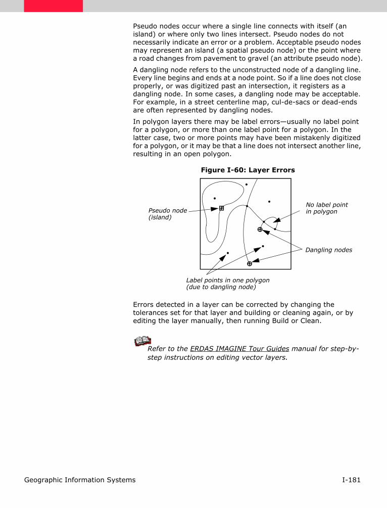
I-181Geographic Information Systems

Pseudo nodes occur where a single line connects with itself (an island) or where only two lines intersect. Pseudo nodes do not necessarily indicate an error or a problem. Acceptable pseudo nodes may represent an island (a spatial pseudo node) or the point where a road changes from pavement to gravel (an attribute pseudo node).

A dangling node refers to the unconstructed node of a dangling line. Every line begins and ends at a node point. So if a line does not close properly, or was digitized past an intersection, it registers as a dangling node. In some cases, a dangling node may be acceptable. For example, in a street centerline map, cul-de-sacs or dead-ends are often represented by dangling nodes.

In polygon layers there may be label errors—usually no label point for a polygon, or more than one label point for a polygon. In the latter case, two or more points may have been mistakenly digitized for a polygon, or it may be that a line does not intersect another line, resulting in an open polygon.

Figure I-60: Layer Errors

Errors detected in a layer can be corrected by changing the tolerances set for that layer and building or cleaning again, or by editing the layer manually, then running Build or Clean.

Refer to the ERDAS IMAGINE Tour Guides manual for step-by-step instructions on editing vector layers.

Label points in one polygon (due to dangling node)

Dangling nodes

No label pointin polygonPseudo node

(island)

I-182 Geographic Information Systems

I-183Cartography

Cartography

Introduction Maps and mapping are the subject of the art and science known as cartography—creating two-dimensional representations of our three-dimensional Earth. These representations were once hand-drawn with paper and pen. But now, map production is largely automated—and the final output is not always paper. The capabilities of a computer system are invaluable to map users, who often need to know much more about an area than can be reproduced on paper, no matter how large that piece of paper is or how small the annotation is. Maps stored on a computer can be queried, analyzed, and updated quickly.

As the veteran GIS and image processing authority, Roger F. Tomlinson, said: “Mapped and related statistical data do form the greatest storehouse of knowledge about the condition of the living space of mankind.” With this thought in mind, it only makes sense that maps be created as accurately as possible and be as accessible as possible.

In the past, map making was carried out by mapping agencies who took the analyst’s (be they surveyors, photogrammetrists, or draftsmen) information and created a map to illustrate that information. But today, in many cases, the analyst is the cartographer and can design his maps to best suit the data and the end user.

This chapter defines some basic cartographic terms and explains how maps are created within the ERDAS IMAGINE environment.

Use the Map Composer to create hardcopy and softcopy maps and presentation graphics.

This chapter concentrates on the production of digital maps. See "Hardcopy Output" on page I-255 for information about printing hardcopy maps.

Types of Maps A map is a graphic representation of spatial relationships on the Earth or other planets. Maps can take on many forms and sizes, depending on the intended use of the map. Maps no longer refer only to hardcopy output. In this manual, the maps discussed begin as digital files and may be printed later as desired.

Some of the different types of maps are defined in Table I-39, “Common Map Scales”.

I-184 Cartography

Map Purpose

Aspect A map that shows the prevailing direction that a slope faces at each pixel. Aspect maps are often color-coded to show the eight major compass directions, or any of 360 degrees.

Base A map portraying background reference information onto which other information is placed. Base maps usually show the location and extent of natural Earth surface features and permanent human-made objects. Raster imagery, orthophotos, and orthoimages are often used as base maps.

Bathymetric A map portraying the shape of a water body or reservoir using isobaths (depth contours).

Cadastral A map showing the boundaries of the subdivisions of land for purposes of describing and recording ownership or taxation.

Choropleth A map portraying properties of a surface using area symbols. Area symbols usually represent categorized classes of the mapped phenomenon.

Composite A map on which the combined information from different thematic maps is presented.

Contour A map in which lines are used to connect points of equal elevation. Lines are often spaced in increments of ten or twenty feet or meters.

Derivative A map created by altering, combining, or analyzing other maps.

Index A reference map that outlines the mapped area, identifies all of the component maps for the area if several map sheets are required, and identifies all adjacent map sheets.

Inset A map that is an enlargement of some congested area of a smaller scale map, and that is usually placed on the same sheet with the smaller scale main map.

Isarithmic A map that uses isorithms (lines connecting points of the same value for any of the characteristics used in the representation of surfaces) to represent a statistical surface. Also called an isometric map.

Isopleth A map on which isopleths (lines representing quantities that cannot exist at a point, such as population density) are used to represent some selected quantity.

Morphometric A map representing morphological features of the Earth’s surface.

Outline A map showing the limits of a specific set of mapping entities, such as counties, NTS quads, etc. Outline maps usually contain a very small number of details over the desired boundaries with their descriptive codes.

Planimetric A map showing only the horizontal position of geographic objects, without topographic features or elevation contours.

Relief Any map that appears to be, or is, three-dimensional. Also called a shaded relief map.

Slope A map that shows changes in elevation over distance. Slope maps are usually color-coded according to the steepness of the terrain at each pixel.

I-185Cartography

In ERDAS IMAGINE, maps are stored as a map file with a .map extension.

Thematic Maps Thematic maps comprise a large portion of the maps that many organizations create. For this reason, this map type is explored in more detail.

Thematic maps may be subdivided into two groups:

• qualitative

• quantitative

A qualitative map shows the spatial distribution or location of a kind of nominal data. For example, a map showing corn fields in the United States would be a qualitative map. It would not show how much corn is produced in each location, or production relative to the other areas.

A quantitative map displays the spatial aspects of numerical data. A map showing corn production (volume) in each area would be a quantitative map. Quantitative maps show ordinal (less than/greater than) and interval/ratio (difference) scale data ( Dent, 1985).

You can create thematic data layers from continuous data (aerial photography and satellite images) using the ERDAS IMAGINE classification capabilities. See "Classification" on page II-99 for more information.

Base Information

Thematic maps should include a base of information so that the reader can easily relate the thematic data to the real world. This base may be as simple as an outline of counties, states, or countries, to something more complex, such as an aerial photograph or satellite image. In the past, it was difficult and expensive to produce maps that included both thematic and continuous data, but technological advances have made this easy.

Thematic A map illustrating the class characterizations of a particular spatial variable (e.g., soils, land cover, hydrology, etc.)

Topographic A map depicting terrain relief.

Viewshed A map showing only those areas visible (or invisible) from a specified point(s). Also called a line-of-sight map or a visibility map.

Map Purpose

I-186 Cartography

For example, in a thematic map showing flood plains in the Mississippi River valley, you could overlay the thematic data onto a line coverage of state borders or a satellite image of the area. The satellite image can provide more detail about the areas bordering the flood plains. This may be valuable information when planning emergency response and resource management efforts for the area. Satellite images can also provide very current information about an area, and can assist you in assessing the accuracy of a thematic image.

In ERDAS IMAGINE, you can include multiple layers in a single map composition. See “Map Composition” on page I-216 for more information about creating maps.

Color Selection

The colors used in thematic maps may or may not have anything to do with the class or category of information shown. Cartographers usually try to use a color scheme that highlights the primary purpose of the map. The map reader’s perception of colors also plays an important role. Most people are more sensitive to red, followed by green, yellow, blue, and purple. Although color selection is left entirely up to the map designer, some guidelines have been established ( Robinson and Sale, 1969).

• When mapping interval or ordinal data, the higher ranks and greater amounts are generally represented by darker colors.

• Use blues for water.

• When mapping elevation data, start with blues for water, greens in the lowlands, ranging up through yellows and browns to reds in the higher elevations. This progression should not be used for series other than elevation.

• In temperature mapping, use red, orange, and yellow for warm temperatures and blue, green, and gray for cool temperatures.

• In land cover mapping, use yellows and tans for dryness and sparse vegetation and greens for lush vegetation.

• Use browns for land forms.

Use the Raster Attributes option in the Viewer to select and modify class colors.

I-187Cartography

Annotation A map is more than just an image(s) on a background. Since a map is a form of communication, it must convey information that may not be obvious by looking at the image. Therefore, maps usually contain several annotation elements to explain the map. Annotation is any explanatory material that accompanies a map to denote graphical features on the map. This annotation may take the form of:

• scale bars

• legends

• neatlines, tick marks, and grid lines

• symbols (north arrows, etc.)

• labels (rivers, mountains, cities, etc.) and descriptive text (title, copyright, credits, production notes, etc.)

The annotation listed above is made up of single elements. The basic annotation elements in ERDAS IMAGINE include:

• rectangles (including squares)

• ellipses (including circles)

• polygons and polylines

• text

These elements can be used to create more complex annotation, such as legends, scale bars, etc. These annotation components are actually groups of the basic elements and can be ungrouped and edited like any other graphic. You can also create your own groups to form symbols that are not in the ERDAS IMAGINE symbol library. (Symbols are discussed in more detail under “Symbols” on page I-193.)

Create annotation using the Annotation tool palette in the Viewer or in a map composition.

How Annotation is Stored

An annotation layer is a set of annotation elements that is drawn in a Viewer or Map Composer window and stored in a file. Annotation that is created in a Viewer window is stored in a separate file from the other data in the Viewer. These annotation files are called overlay files (.ovr extension). Map annotation that is created in a Map Composer window is also stored in an .ovr file, which is named after the map composition. For example, the annotation for a file called lanier.map would be lanier.map.ovr.

I-188 Cartography

Scale Map scale is a statement that relates distance on a map to distance on the Earth’s surface. It is perhaps the most important information on a map, since the level of detail and map accuracy are both factors of the map scale. Scale is directly related to the map extent, or the area of the Earth’s surface to be mapped. If a relatively small area is to be mapped, such as a neighborhood or subdivision, then the scale can be larger. If a large area is to be mapped, such as an entire continent, the scale must be smaller. Generally, the smaller the scale, the less detailed the map can be. As a rule, anything smaller than 1:250,000 is considered small-scale.

Scale can be reported in several ways, including:

• representative fraction

• verbal statement

• scale bar

Representative Fraction

Map scale is often noted as a simple ratio or fraction called a representative fraction. A map in which one inch on the map equals 24,000 inches on the ground could be described as having a scale of 1:24,000 or 1/24,000. The units on both sides of the ratio must be the same.

Verbal Statement

A verbal statement of scale describes the distance on the map to the distance on the ground. A verbal statement describing a scale of 1:1,000,000 is approximately 1 inch to 16 miles. The units on the map and on the ground do not have to be the same in a verbal statement. One-inch and 6-inch maps of the British Ordnance Survey are often referred to by this method (1 inch to 1 mile, 6 inches to 1 mile) ( Robinson and Sale, 1969).

Scale Bars

A scale bar is a graphic annotation element that describes map scale. It shows the distance on paper that represents a geographical distance on the map. Maps often include more than one scale bar to indicate various measurement systems, such as kilometers and miles.

Figure I-61: Sample Scale Bars

Kilometers

Miles

1 0 1 2 3 4

1 0 1 2

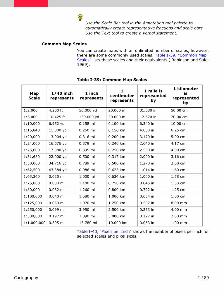
I-189Cartography

Use the Scale Bar tool in the Annotation tool palette to automatically create representative fractions and scale bars. Use the Text tool to create a verbal statement.

Common Map Scales

You can create maps with an unlimited number of scales, however, there are some commonly used scales. Table I-39, “Common Map Scales” lists these scales and their equivalents ( Robinson and Sale, 1969).

Table I-40, “Pixels per Inch” shows the number of pixels per inch for selected scales and pixel sizes.

Table I-39: Common Map Scales

Map Scale

1/40 inch represents

1 inch represents

1 centimeter represents

1 mile is represented

by

1 kilometer is

represented by

1:2,000 4.200 ft 56.000 yd 20.000 m 31.680 in 50.00 cm

1:5,000 10.425 ft 139.000 yd 50.000 m 12.670 in 20.00 cm

1:10,000 6.952 yd 0.158 mi 0.100 km 6.340 in 10.00 cm

1:15,840 11.000 yd 0.250 mi 0.156 km 4.000 in 6.25 cm

1:20,000 13.904 yd 0.316 mi 0.200 km 3.170 in 5.00 cm

1:24,000 16.676 yd 0.379 mi 0.240 km 2.640 in 4.17 cm

1:25,000 17.380 yd 0.395 mi 0.250 km 2.530 in 4.00 cm

1:31,680 22.000 yd 0.500 mi 0.317 km 2.000 in 3.16 cm

1:50,000 34.716 yd 0.789 mi 0.500 km 1.270 in 2.00 cm

1:62,500 43.384 yd 0.986 mi 0.625 km 1.014 in 1.60 cm

1:63,360 0.025 mi 1.000 mi 0.634 km 1.000 in 1.58 cm

1:75,000 0.030 mi 1.180 mi 0.750 km 0.845 in 1.33 cm

1:80,000 0.032 mi 1.260 mi 0.800 km 0.792 in 1.25 cm

1:100,000 0.040 mi 1.580 mi 1.000 km 0.634 in 1.00 cm

1:125,000 0.050 mi 1.970 mi 1.250 km 0.507 in 8.00 mm

1:250,000 0.099 mi 3.950 mi 2.500 km 0.253 in 4.00 mm

1:500,000 0.197 mi 7.890 mi 5.000 km 0.127 in 2.00 mm

1:1,000,000 0.395 mi 15.780 mi 10.000 km 0.063 in 1.00 mm

I-190 Cartography

Courtesy of D. Cunningham and D. Way, The Ohio State University

Table I-40: Pixels per Inch

Pixel

Size (m)

SCALE

1”=100’

1:1200

1”=200’

1:2400

1”=500’

1:6000

1”=1000’

1:12000

1”=1500’

1:18000

1”=2000’

1:24000

1”=4167’

1:50000

1”=1 mile

1:63360

1 30.49 60.96 152.40 304.80 457.20 609.60 1270.00 1609.35

2 15.24 30.48 76.20 152.40 228.60 304.80 635.00 804.67

2.5 12.13 24.38 60.96 121.92 182.88 243.84 508.00 643.74

5 6.10 12.19 30.48 60.96 91.44 121.92 254.00 321.87

10 3.05 6.10 15.24 30.48 45.72 60.96 127.00 160.93

15 2.03 4.06 10.16 20.32 30.48 40.64 84.67 107.29

20 1.52 3.05 7.62 15.24 22.86 30.48 63.50 80.47

25 1.22 2.44 6.10 12.19 18.29 24.38 50.80 64.37

30 1.02 2.03 5.08 10.16 15.240 20.32 42.33 53.64

35 .87 1.74 4.35 8.71 13.08 17.42 36.29 45.98

40 .76 1.52 3.81 7.62 11.43 15.24 31.75 40.23

45 .68 1.35 3.39 6.77 10.16 13.55 28.22 35.76

50 .61 1.22 3.05 6.10 9.14 12.19 25.40 32.19

75 .41 .81 2.03 4.06 6.10 8.13 16.93 21.46

100 .30 .61 1.52 3.05 4.57 6.10 12.70 16.09

150 .20 .41 1.02 2.03 3.05 4.06 8.47 10.73

200 .15 .30 .76 1.52 2.29 3.05 6.35 8.05

250 .12 .24 .61 1.22 1.83 2.44 5.08 6.44

300 .10 .30 .51 1.02 1.52 2.03 4.23 5.36

350 .09 .17 .44 .87 1.31 1.74 3.63 4.60

400 .08 .15 .38 .76 1.14 1.52 3.18 4.02

450 .07 .14 .34 .68 1.02 1.35 2.82 3.58

500 .06 .12 .30 .61 .91 1.22 2.54 3.22

600 .05 .10 .25 .51 .76 1.02 2.12 2.69

700 .04 .09 .22 .44 .65 .87 1.81 2.30

800 .04 .08 .19 .38 .57 .76 1.59 2.01

900 .03 .07 .17 .34 .51 .68 1.41 1.79

1000 .03 .06 .15 .30 .46 .61 1.27 1.61

I-191Cartography

Table I-41, “Acres and Hectares per Pixel” lists the number of acres and hectares per pixel for various pixel sizes.

Courtesy of D. Cunningham and D. Way, The Ohio State University

Table I-41: Acres and Hectares per Pixel

Pixel Size (m) Acres Hectares

1 0.0002 0.0001

2 0.0010 0.0004

2.5 0.0015 0.0006

5 0.0062 0.0025

10 0.0247 0.0100

15 0.0556 0.0225

20 0.0988 0.0400

25 0.1544 0.0625

30 0.2224 0.0900

35 0.3027 0.1225

40 0.3954 0.1600

45 0.5004 0.2025

50 0.6178 0.2500

75 1.3900 0.5625

100 2.4710 1.0000

150 5.5598 2.2500

200 9.8842 4.0000

250 15.4440 6.2500

300 22.2394 9.0000

350 30.2703 12.2500

400 39.5367 16.0000

450 50.0386 20.2500

500 61.7761 25.0000

600 88.9576 36.0000

700 121.0812 49.0000

800 158.1468 64.0000

900 200.1546 81.0000

1000 247.1044 100.0000

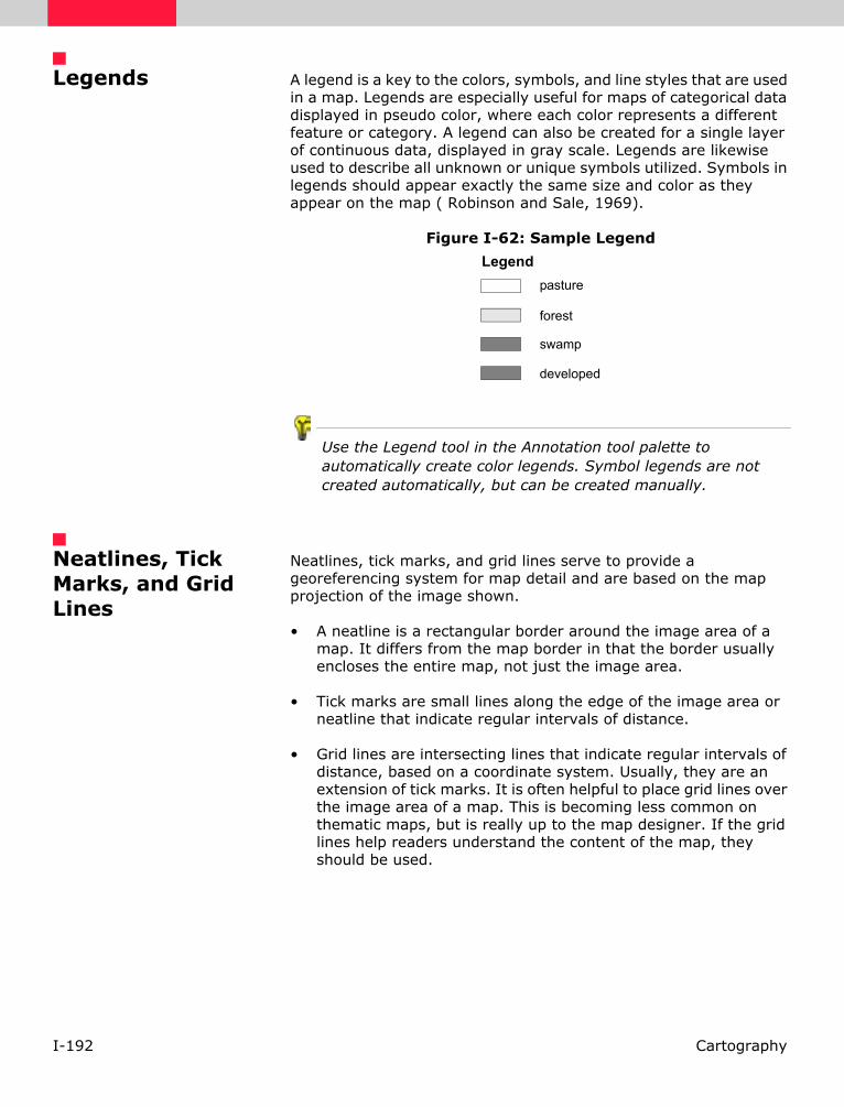
I-192 Cartography

Legends A legend is a key to the colors, symbols, and line styles that are used in a map. Legends are especially useful for maps of categorical data displayed in pseudo color, where each color represents a different feature or category. A legend can also be created for a single layer of continuous data, displayed in gray scale. Legends are likewise used to describe all unknown or unique symbols utilized. Symbols in legends should appear exactly the same size and color as they appear on the map ( Robinson and Sale, 1969).

Figure I-62: Sample Legend

Use the Legend tool in the Annotation tool palette to automatically create color legends. Symbol legends are not created automatically, but can be created manually.

Neatlines, Tick Marks, and Grid Lines

Neatlines, tick marks, and grid lines serve to provide a georeferencing system for map detail and are based on the map projection of the image shown.

• A neatline is a rectangular border around the image area of a map. It differs from the map border in that the border usually encloses the entire map, not just the image area.

• Tick marks are small lines along the edge of the image area or neatline that indicate regular intervals of distance.

• Grid lines are intersecting lines that indicate regular intervals of distance, based on a coordinate system. Usually, they are an extension of tick marks. It is often helpful to place grid lines over the image area of a map. This is becoming less common on thematic maps, but is really up to the map designer. If the grid lines help readers understand the content of the map, they should be used.

pasture

forest

swamp

developed

Legend

I-193Cartography

Figure I-63: Sample Neatline, Tick Marks, and Grid Lines

Grid lines may also be referred to as a graticule.

Graticules are discussed in more detail in “Projections”on page I-198.

Use the Grid/Tick tool in the Annotation tool palette to create neatlines, tick marks, and grid lines. Tick marks and grid lines can also be created over images displayed in a Viewer. See the On-Line Help for instructions.

Symbols Since maps are a greatly reduced version of the real-world, objects cannot be depicted in their true shape or size. Therefore, a set of symbols is devised to represent real-world objects. There are two major classes of symbols:

• replicative

• abstract

Replicative symbols are designed to look like their real-world counterparts; they represent tangible objects, such as coastlines, trees, railroads, and houses. Abstract symbols usually take the form of geometric shapes, such as circles, squares, and triangles. They are traditionally used to represent amounts that vary from place to place, such as population density, amount of rainfall, etc. ( Dent, 1985).

Both replicative and abstract symbols are composed of one or more of the following annotation elements:

• point

neatline

tick marksgrid lines

I-194 Cartography

• line

• area

Symbol Types

These basic elements can be combined to create three different types of replicative symbols:

• plan—formed after the basic outline of the object it represents. For example, the symbol for a house might be a square, because most houses are rectangular.

• profile—formed like the profile of an object. Profile symbols generally represent vertical objects, such as trees, windmills, oil wells, etc.

• function—formed after the activity that a symbol represents. For example, on a map of a state park, a symbol of a tent would indicate the location of a camping area.

Figure I-64: Sample Symbols

Symbols can have different sizes, colors, and patterns to indicate different meanings within a map. The use of size, color, and pattern generally shows qualitative or quantitative differences among areas marked. For example, if a circle is used to show cities and towns, larger circles would be used to show areas with higher population. A specific color could be used to indicate county seats. Since symbols are not drawn to scale, their placement is crucial to effective communication.

Use the Symbol tool in the Annotation tool palette and the symbol library to place symbols in maps.

Labels and Descriptive Text

Place names and other labels convey important information to the reader about the features on the map. Any features that help orient the reader or are important to the content of the map should be labeled. Descriptive text on a map can include the map title and subtitle, copyright information, captions, credits, production notes, or other explanatory material.

Plan Profile Function

I-195Cartography

Title

The map title usually draws attention by virtue of its size. It focuses the reader’s attention on the primary purpose of the map. The title may be omitted, however, if captions are provided outside of the image area ( Dent, 1985).

Credits

Map credits (or source information) can include the data source and acquisition date, accuracy information, and other details that are required or helpful to readers. For example, if you include data that you do not own in a map, you must give credit to the owner.

Use the Text tool in the Annotation tool palette to add labels and descriptive text to maps.

Typography and Lettering The choice of type fonts and styles and how names are lettered can make the difference between a clear and attractive map and a jumble of imagery and text. As with many other aspects of map design, this is a very subjective area and many organizations already have guidelines to use. This section is intended as an introduction to the concepts involved and to convey traditional guidelines, where available.

If your organization does not have a set of guidelines for the appearance of maps and you plan to produce many in the future, it would be beneficial to develop a style guide specifically for mapping. This ensures that all of the maps produced follow the same conventions, regardless of who actually makes the map.

ERDAS IMAGINE enables you to make map templates to facilitate the development of map standards within your organization.

Type Styles

Type style refers to the appearance of the text and may include font, size, and style (bold, italic, underline, etc.). Although the type styles used in maps are purely a matter of the designer’s taste, the following techniques help to make maps more legible ( Robinson and Sale, 1969; Dent, 1985).

• Do not use too many different typefaces in a single map. Generally, one or two styles are enough when also using the variations of those type faces (e.g., bold, italic, underline, etc.). When using two typefaces, use a serif and a sans serif, rather than two different serif fonts or two different sans serif fonts [e.g., Sans (sans serif) and Roman (serif) could be used together in one map].

• Avoid ornate text styles because they can be difficult to read.

I-196 Cartography

• Exercise caution in using very thin letters that may not reproduce well. On the other hand, using letters that are too bold may obscure important information in the image.

• Use different sizes of type for showing varying levels of importance. For example, on a map with city and town labels, city names are usually in a larger type size than the town names. Use no more than four to six different type sizes.

• Put more important text in labels, titles, and names in all capital letters and lesser important text in lowercase with initial capitals. This is a matter of personal preference, although names in which the letters must be spread out across a large area are better in all capital letters. (Studies have found that capital letters are more difficult to read, therefore lowercase letters might improve the legibility of the map.)

• In the past, hydrology, landform, and other natural features were labeled in italic. However, this is not strictly adhered to by map makers today, although water features are still nearly always labeled in italic.

Figure I-65: Sample Sans Serif and Serif Typefaces with Various Styles Applied

Use the Styles dialog to adjust the style of text.

Lettering

Lettering refers to the way in which place names and other labels are added to a map. Letter spacing, orientation, and position are the three most important factors in lettering. Here again, there are no set rules for how lettering is to appear. Much is determined by the purpose of the map and the end user. Many organizations have developed their own rules for lettering. Here is a list of guidelines that have been used by cartographers in the past ( Robinson and Sale, 1969; Dent, 1985).

• Names should be either entirely on land or water—not overlapping both.

Sans 10 pt regular

Sans 10 pt italic

Sans 10 pt bold

Sans 10 pt bold italic

SANS 10 PT ALL CAPS

Roman 10 pt regular

Roman 10 pt italic

Roman 10 pt bold

Roman 10 pt bold italic

ROMAN 10 PT ALL CAPS

Sans Serif Serif

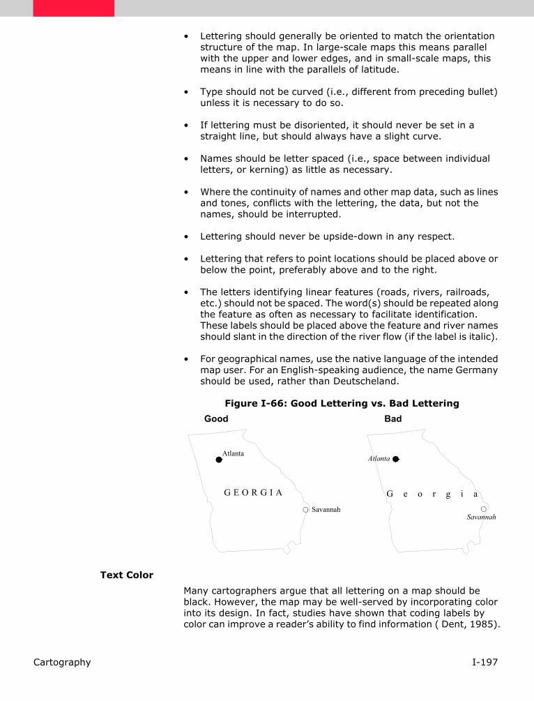
I-197Cartography

• Lettering should generally be oriented to match the orientation structure of the map. In large-scale maps this means parallel with the upper and lower edges, and in small-scale maps, this means in line with the parallels of latitude.

• Type should not be curved (i.e., different from preceding bullet) unless it is necessary to do so.

• If lettering must be disoriented, it should never be set in a straight line, but should always have a slight curve.

• Names should be letter spaced (i.e., space between individual letters, or kerning) as little as necessary.

• Where the continuity of names and other map data, such as lines and tones, conflicts with the lettering, the data, but not the names, should be interrupted.

• Lettering should never be upside-down in any respect.

• Lettering that refers to point locations should be placed above or below the point, preferably above and to the right.

• The letters identifying linear features (roads, rivers, railroads, etc.) should not be spaced. The word(s) should be repeated along the feature as often as necessary to facilitate identification. These labels should be placed above the feature and river names should slant in the direction of the river flow (if the label is italic).

• For geographical names, use the native language of the intended map user. For an English-speaking audience, the name Germany should be used, rather than Deutscheland.

Figure I-66: Good Lettering vs. Bad Lettering

Text Color

Many cartographers argue that all lettering on a map should be black. However, the map may be well-served by incorporating color into its design. In fact, studies have shown that coding labels by color can improve a reader’s ability to find information ( Dent, 1985).

Atlanta

G E O R G I A

Good

Atlanta

G e o r g i aSavannah

Savannah

Bad

I-198 Cartography

Projections

This section is adapted from “Map Projections for Use with the Geographic Information System” by Lee and Walsh ( Lee and Walsh, 1984).

A map projection is the manner in which the spherical surface of the Earth is represented on a flat (two-dimensional) surface. This can be accomplished by direct geometric projection or by a mathematically derived transformation. There are many kinds of projections, but all involve transfer of the distinctive global patterns of parallels of latitude and meridians of longitude onto an easily flattened surface, or developable surface.

The three most common developable surfaces are the cylinder, cone, and plane (Figure I-67 on page I-200). A plane is already flat, while a cylinder or cone may be cut and laid out flat, without stretching. Thus, map projections may be classified into three general families: cylindrical, conical, and azimuthal or planar.

Map projections are selected in the Projection Chooser. For more information about the Projection Chooser, see the ERDAS IMAGINE On-Line Help.

Properties of Map Projections

Regardless of what type of projection is used, it is inevitable that some error or distortion occurs in transforming a spherical surface into a flat surface. Ideally, a distortion-free map has four valuable properties:

• conformality

• equivalence

• equidistance

• true direction

Each of these properties is explained below. No map projection can be true in all of these properties. Therefore, each projection is devised to be true in selected properties, or most often, a compromise among selected properties. Projections that compromise in this manner are known as compromise projections.

I-199Cartography

Conformality is the characteristic of true shape, wherein a projection preserves the shape of any small geographical area. This is accomplished by exact transformation of angles around points. One necessary condition is the perpendicular intersection of grid lines as on the globe. The property of conformality is important in maps which are used for analyzing, guiding, or recording motion, as in navigation. A conformal map or projection is one that has the property of true shape.

Equivalence is the characteristic of equal area, meaning that areas on one portion of a map are in scale with areas in any other portion. Preservation of equivalence involves inexact transformation of angles around points and thus, is mutually exclusive with conformality except along one or two selected lines. The property of equivalence is important in maps that are used for comparing density and distribution data, as in populations.

Equidistance is the characteristic of true distance measuring. The scale of distance is constant over the entire map. This property can be fulfilled on any given map from one, or at most two, points in any direction or along certain lines. Equidistance is important in maps that are used for analyzing measurements (i.e., road distances). Typically, reference lines such as the equator or a meridian are chosen to have equidistance and are termed standard parallels or standard meridians.

True direction is characterized by a direction line between two points that crosses reference lines (e.g., meridians) at a constant angle or azimuth. An azimuth is an angle measured clockwise from a meridian, going north to east. The line of constant or equal direction is termed a rhumb line.

The property of constant direction makes it comparatively easy to chart a navigational course. However, on a spherical surface, the shortest surface distance between two points is not a rhumb line, but a great circle, being an arc of a circle whose center is the center of the Earth. Along a great circle, azimuths constantly change (unless the great circle is the equator or a meridian).

Thus, a more desirable property than true direction may be where great circles are represented by straight lines. This characteristic is most important in aviation. Note that all meridians are great circles, but the only parallel that is a great circle is the equator.

I-200 Cartography

Figure I-67: Projection Types

Projection Types Although a great number of projections have been devised, the majority of them are geometric or mathematical variants of the basic direct geometric projection families described below. Choice of the projection to be used depends upon the true property or combination of properties desired for effective cartographic analysis.

Azimuthal Projections

Azimuthal projections, also called planar projections, are accomplished by drawing lines from a given perspective point through the globe onto a tangent plane. This is conceptually equivalent to tracing a shadow of a figure cast by a light source. A tangent plane intersects the global surface at only one point and is perpendicular to a line passing through the center of the sphere. Thus, these projections are symmetrical around a chosen center or central meridian. Choice of the projection center determines the aspect, or orientation, of the projection surface.

Azimuthal projections may be centered:

Regular Cylindrical

Transverse Cylindrical

Oblique Cylindrical

Regular Conic

Polar Azimuthal(planar)

Oblique Azimuthal(planar)

I-201Cartography

• on the poles (polar aspect)

• at a point on the equator (equatorial aspect)

• at any other orientation (oblique aspect)

The origin of the projection lines—that is, the perspective point—may also assume various positions. For example, it may be:

• the center of the Earth (gnomonic)

• an infinite distance away (orthographic)

• on the Earth’s surface, opposite the projection plane (stereographic)

Conical Projections

Conical projections are accomplished by intersecting, or touching, a cone with the global surface and mathematically projecting lines onto this developable surface.

A tangent cone intersects the global surface to form a circle. Along this line of intersection, the map is error-free and possess equidistance. Usually, this line is a parallel, termed the standard parallel.

Cones may also be secant, and intersect the global surface, forming two circles that possess equidistance. In this case, the cone slices underneath the global surface, between the standard parallels. Note that the use of the word secant, in this instance, is only conceptual and not geometrically accurate. Conceptually, the conical aspect may be polar, equatorial, or oblique. Only polar conical projections are supported in ERDAS IMAGINE.

Figure I-68: Tangent and Secant Cones

Cylindrical Projections

Cylindrical projections are accomplished by intersecting, or touching, a cylinder with the global surface. The surface is mathematically projected onto the cylinder, which is then cut and unrolled.

Secanttwo standard parallels

Tangentone standard parallel

I-202 Cartography

A tangent cylinder intersects the global surface on only one line to form a circle, as with a tangent cone. This central line of the projection is commonly the equator and possesses equidistance.

If the cylinder is rotated 90 degrees from the vertical (i.e., the long axis becomes horizontal), then the aspect becomes transverse, wherein the central line of the projection becomes a chosen standard meridian as opposed to a standard parallel. A secant cylinder, one slightly less in diameter than the globe, has two lines possessing equidistance.

Figure I-69: Tangent and Secant Cylinders

Perhaps the most famous cylindrical projection is the Mercator, which became the standard navigational map. Mercator possesses true direction and conformality.

Other Projections

The projections discussed so far are projections that are created by projecting from a sphere (the Earth) onto a plane, cone, or cylinder. Many other projections cannot be created so easily.

Modified projections are modified versions of another projection. For example, the Space Oblique Mercator projection is a modification of the Mercator projection. These modifications are made to reduce distortion, often by including additional standard lines or a different pattern of distortion.

Pseudo projections have only some of the characteristics of another class projection. For example, the Sinusoidal is called a pseudocylindrical projection because all lines of latitude are straight and parallel, and all meridians are equally spaced. However, it cannot truly be a cylindrical projection, because all meridians except the central meridian are curved. This results in the Earth appearing oval instead of rectangular (Environmental Systems Research Institute, 1991).

Geographical and Planar Coordinates

Map projections require a point of reference on the Earth’s surface. Most often this is the center, or origin, of the projection. This point is defined in two coordinate systems:

• geographical

Tangentone standard parallel

Secanttwo standard parallels

I-203Cartography

• planar

Geographical

Geographical, or spherical, coordinates are based on the network of latitude and longitude (Lat/Lon) lines that make up the graticule of the Earth. Within the graticule, lines of longitude are called meridians, which run north/south, with the prime meridian at 0° (Greenwich, England). Meridians are designated as 0° to 180°, east or west of the prime meridian. The 180° meridian (opposite the prime meridian) is the International Dateline.

Lines of latitude are called parallels, which run east/west. Parallels are designated as 0° at the equator to 90° at the poles. The equator is the largest parallel. Latitude and longitude are defined with respect to an origin located at the intersection of the equator and the prime meridian. Lat/Lon coordinates are reported in degrees, minutes, and seconds. Map projections are various arrangements of the Earth’s latitude and longitude lines onto a plane.

Planar

Planar, or Cartesian, coordinates are defined by a column and row position on a planar grid (X,Y). The origin of a planar coordinate system is typically located south and west of the origin of the projection. Coordinates increase from 0,0 going east and north. The origin of the projection, being a false origin, is defined by values of false easting and false northing. Grid references always contain an even number of digits, and the first half refers to the easting and the second half the northing.

In practice, this eliminates negative coordinate values and allows locations on a map projection to be defined by positive coordinate pairs. Values of false easting are read first and may be in meters or feet.

Available Map Projections

In ERDAS IMAGINE, map projection information appears in the Projection Chooser, which is used to georeference images and to convert map coordinates from one type of projection to another. The Projection Chooser provides the following projections:

USGS Projections

• Alaska Conformal

• Albers Conical Equal Area

• Azimuthal Equidistant

• Behrmann

• Bonne

I-204 Cartography

• Cassini

• Eckert I

• Eckert II

• Eckert III

• Eckert IV

• Eckert V

• Eckert VI

• EOSAT SOM

• Equidistant Conic

• Equidistant Cylindrical

• Equirectangular (Plate Carrée)

• Gall Stereographic

• Gauss Kruger

• General Vertical Near-side Perspective

• Geographic (Lat/Lon)

• Gnomonic

• Hammer

• Interrupted Goode Homolosine

• Interrupted Mollweide

• Lambert Azimuthal Equal Area

• Lambert Conformal Conic

• Loximuthal

• Mercator

• Miller Cylindrical

• Modified Transverse Mercator

• Mollweide

• New Zealand Map Grid

I-205Cartography

• Oblated Equal Area

• Oblique Mercator (Hotine)

• Orthographic

• Plate Carrée

• Polar Stereographic

• Polyconic

• Quartic Authalic

• Robinson

• RSO

• Sinusoidal

• Space Oblique Mercator

• Space Oblique Mercator (Formats A & B)

• State Plane

• Stereographic

• Stereographic (Extended)

• Transverse Mercator

• Two Point Equidistant

• UTM

• Van der Grinten I

• Wagner IV

• Wagner VII

• Winkel I

External Projections

• Albers Equal Area (see "Albers Conical Equal Area" on page I-269)

• Azimuthal Equidistant (see "Azimuthal Equidistant" on page I-272)

• Bipolar Oblique Conic Conformal

I-206 Cartography

• Cassini-Soldner

• Conic Equidistant (see "Equidistant Conic" on page I-294)

• Laborde Oblique Mercator

• Lambert Azimuthal Equal Area (see "Lambert Azimuthal Equal Area" on page I-312)

• Lambert Conformal Conic (see "Lambert Conformal Conic" on page I-315)

• Mercator (see "Mercator" on page I-320)

• Minimum Error Conformal

• Modified Polyconic

• Modified Stereographic

• Mollweide Equal Area (see "Mollweide" on page I-327)

• Oblique Mercator (see "Oblique Mercator (Hotine)" on page I-331)

• Orthographic (see "Orthographic" on page I-334)

• Plate Carrée (see "Equirectangular (Plate Carrée)" on page I-297)

• Rectified Skew Orthomorphic (see "RSO" on page I-347)

• Regular Polyconic (see "Polyconic" on page I-341)

• Robinson Pseudocylindrical (see "Robinson" on page I-345)

• Sinusoidal (see "Sinusoidal" on page I-348)

• Southern Orientated Gauss Conformal

• Stereographic (see "Stereographic" on page I-363)

• Swiss Cylindrical

• Stereographic (Oblique) (see "Stereographic" on page I-363)

• Transverse Mercator (see "Transverse Mercator" on page I-367)

• Universal Transverse Mercator (see "UTM" on page I-371)

• Van der Grinten (see "Van der Grinten I" on page I-374)

• Winkel’s Tripel

I-207Cartography

Choice of the projection to be used depends upon the desired major property and the region to be mapped (see Table I-42 on page I-207). After choosing the desired map projection, several parameters are required for its definition (see Table I-43 on page I-208). These parameters fall into three general classes: (1) definition of the spheroid, (2) definition of the surface viewing window, and (3) definition of scale.

For each map projection, a menu of spheroids displays, along with appropriate prompts that enable you to specify these parameters.

Units

Use the units of measure that are appropriate for the map projection type.

• Lat/Lon coordinates are expressed in decimal degrees. When prompted, you can use the DD function to convert coordinates in degrees, minutes, seconds format to decimal. For example, for 30°51’12’’:

dd(30,51,12) = 30.85333 -dd(30,51,12) = -30.85333

or

30:51:12 = 30.85333You can also enter Lat/Lon coordinates in radians.

• State Plane coordinates are expressed in feet or meters.

• All other coordinates are expressed in meters.

Note also that values for longitude west of Greenwich, England, and values for latitude south of the equator are to be entered as negatives.

Table I-42: Map Projections

Map projection Construction Property Use

0 Geographic N/A N/A Data entry, spherical coordinates

1 Universal Transverse Mercator Cylinder (see #9)

Conformal Data entry, plane coordinates

2 State Plane (see #4, 7,9,20)

Conformal Data entry, plane coordinates

3 Albers Conical Equal Area Cone Equivalent Middle latitudes, E-W expanses

4 Lambert Conformal Conic Cone Conformal True Direction

Middle latitudes, E-W expanses flight (straight great circles)

I-208 Cartography

5 Mercator Cylinder Conformal True Direction

Nonpolar regions, navigation (straight rhumb lines)

6 Polar Stereographic Plane Conformal Polar regions

7 Polyconic Cone Compromise N-S expanses

8 Equidistant Conic Cone Equidistant Middle latitudes, E-W expanses

9 Transverse Mercator Cylinder Conformal N-S expanses

10 Stereographic Plane Conformal Hemispheres, continents

11 Lambert Azimuthal Equal Area

Plane Equivalent Square or round expanses

12 Azimuthal Equidistant Plane Equidistant Polar regions, radio/seismic work (straight great circles)

13 Gnomonic Plane Compromise Navigation, seismic work (straight great circles)

14 Orthographic Plane Compromise Globes, pictorial

15 General Vertical Near-Side Perspective

Plane Compromise Hemispheres or less

16 Sinusoidal Pseudo-Cylinder Equivalent N-S expanses or equatorial regions

17 Equirectangular Cylinder Compromise City maps, computer plotting (simplistic)

18 Miller Cylindrical Cylinder Compromise World maps

19 Van der Grinten I N/A Compromise World maps

20 Oblique Mercator Cylinder Conformal Oblique expanses (e.g., Hawaiian islands), satellite tracking

21 Space Oblique Mercator Cylinder Conformal Mapping of Landsat imagery

22 Modified Transverse Mercator

Cylinder Conformal Alaska

Table I-43: Projection Parameters

Projection type (#)1

Parameter 3 4 5 6 7 8b 9 10 11 12 13 14 15 16 17 18 19 202 21b 22

Definition of Spheroid

Spheroid selections

• • • • • • • • • • • • • • • • • • •

Definition of Surface Viewing Window

Table I-42: Map Projections (Continued)

Map projection Construction Property Use

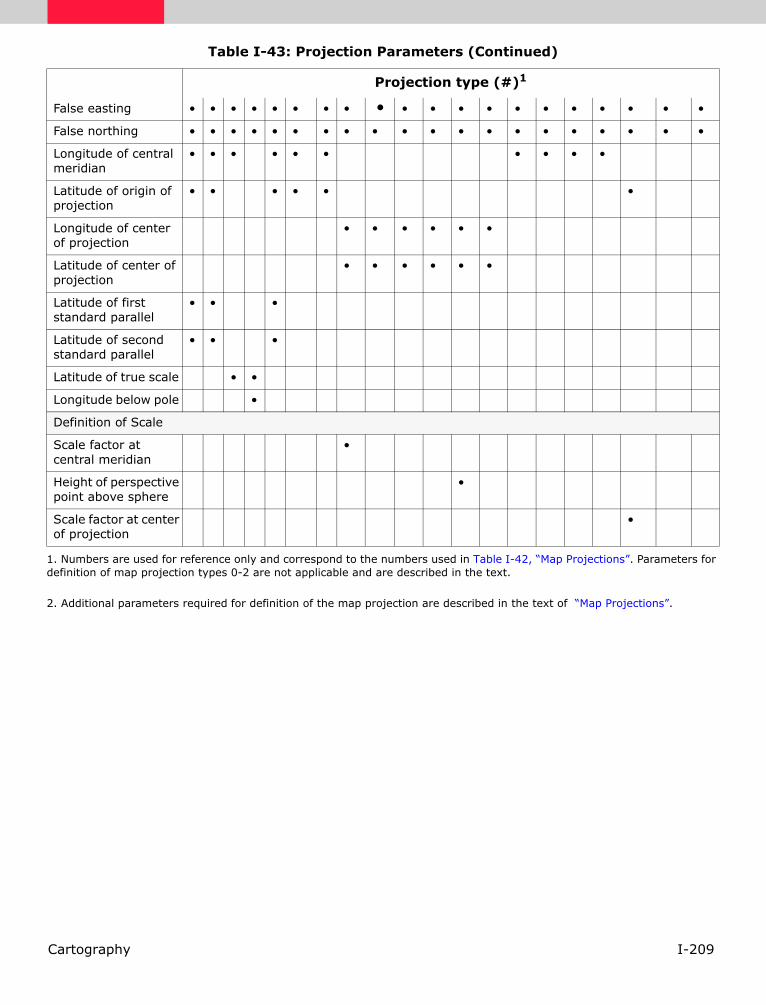
I-209Cartography

False easting • • • • • • • • • • • • • • • • • • • •

False northing • • • • • • • • • • • • • • • • • • • •

Longitude of central meridian

• • • • • • • • • •

Latitude of origin of projection

• • • • • •

Longitude of center of projection

• • • • • •

Latitude of center of projection

• • • • • •

Latitude of first standard parallel

• • •

Latitude of second standard parallel

• • •

Latitude of true scale • •

Longitude below pole •

Definition of Scale

Scale factor at central meridian

•

Height of perspective point above sphere

•

Scale factor at center of projection

•

1. Numbers are used for reference only and correspond to the numbers used in Table I-42, “Map Projections”. Parameters for definition of map projection types 0-2 are not applicable and are described in the text.

2. Additional parameters required for definition of the map projection are described in the text of “Map Projections”.

Table I-43: Projection Parameters (Continued)

Projection type (#)1

I-210 Cartography

Choosing a Map Projection

Map Projection Uses in a GIS

Selecting a map projection for the GIS database enables you to ( Maling, 1992):

• decide how to best display the area of interest or illustrate the results of analysis

• register all imagery to a single coordinate system for easier comparisons

• test the accuracy of the information and perform measurements on the data

Deciding Factors Depending on your applications and the uses for the maps created, one or several map projections may be used. Many factors must be weighed when selecting a projection, including:

• type of map

• special properties that must be preserved

• types of data to be mapped

• map accuracy

• scale

If you are mapping a relatively small area, virtually any map projection is acceptable. In mapping large areas (entire countries, continents, and the world), the choice of map projection becomes more critical. In small areas, the amount of distortion in a particular projection is barely, if at all, noticeable. In large areas, there may be little or no distortion in the center of the map, but distortion increases outward toward the edges of the map.

Guidelines Since the sixteenth century, there have been three fundamental rules regarding map projection use ( Maling, 1992):

• if the country to be mapped lies in the tropics, use a cylindrical projection

• if the country to be mapped lies in the temperate latitudes, use a conical projection

• if the map is required to show one of the polar regions, use an azimuthal projection

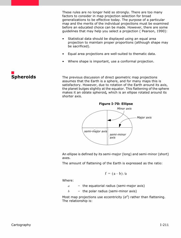
I-211Cartography

These rules are no longer held so strongly. There are too many factors to consider in map projection selection for broad generalizations to be effective today. The purpose of a particular map and the merits of the individual projections must be examined before an educated choice can be made. However, there are some guidelines that may help you select a projection ( Pearson, 1990):

• Statistical data should be displayed using an equal area projection to maintain proper proportions (although shape may be sacrificed).

• Equal area projections are well-suited to thematic data.

• Where shape is important, use a conformal projection.

Spheroids The previous discussion of direct geometric map projections assumes that the Earth is a sphere, and for many maps this is satisfactory. However, due to rotation of the Earth around its axis, the planet bulges slightly at the equator. This flattening of the sphere makes it an oblate spheroid, which is an ellipse rotated around its shorter axis.

Figure I-70: Ellipse

An ellipse is defined by its semi-major (long) and semi-minor (short) axes.

The amount of flattening of the Earth is expressed as the ratio:

Where:

a = the equatorial radius (semi-major axis)

b = the polar radius (semi-minor axis)

Most map projections use eccentricity (e2) rather than flattening. The relationship is:

Minor axis

Major axis

semi-minor axis

semi-major axis

f a b–( ) a⁄=

I-212 Cartography

The flattening of the Earth is about 1 part in 300, and becomes significant in map accuracy at a scale of 1:100,000 or larger.

Calculation of a map projection requires definition of the spheroid (or ellipsoid) in terms of the length of axes and eccentricity squared (or radius of the reference sphere). Several principal spheroids are in use by one or more countries. Differences are due primarily to calculation of the spheroid for a particular region of the Earth’s surface. Only recently have satellite tracking data provided spheroid determinations for the entire Earth. However, these spheroids may not give the best fit for a particular region. In North America, the spheroid in use is the Clarke 1866 for NAD27 and GRS 1980 for NAD83 (State Plane).

If other regions are to be mapped, different projections should be used. Upon choosing a desired projection type, you have the option to choose from the following list of spheroids:

• Airy

• Australian National

• Bessel

• Clarke 1866

• Clarke 1880

• Everest

• GRS 1980

• Helmert

• Hough

• International 1909

• Krasovsky

• Mercury 1960

• Modified Airy

• Modified Everest

• Modified Mercury 1968

• New International 1967

• Southeast Asia

e2 2f f2–=

I-213Cartography

• Sphere of Nominal Radius of Earth

• Sphere of Radius 6370977m

• Walbeck

• WGS 66

• WGS 72

• WGS 84

The spheroids listed above are the most commonly used. There are many other spheroids available, and they are listed in the Projection Chooser. These additional spheroids are not documented in this manual. You can use the IMAGINE Developers’ Toolkit to add your own map projections and spheroids to ERDAS IMAGINE.

The semi-major and semi-minor axes of all supported spheroids are listed in Table I-44 on page I-214, as well as the principal uses of these spheroids.

I-214 Cartography

Table I-44: Spheroids for use with ERDAS IMAGINE

Spheroid Semi-Major Axis

Semi-Minor Axis Use

165 6378165.0 6356783.0 Global

Airy (1940) 6377563.0 6356256.91 England

Airy Modified (1849) Ireland

Australian National (1965) 6378160.0 6356774.719 Australia

Bessel (1841) 6377397.155 6356078.96284 Central Europe, Chile, and Indonesia

Bessell (Namibia) 6377483.865 6356165.383 Namibia

Clarke 1858 6378293.0 6356619.0 Global

Clarke 1866 6378206.4 6356583.8 North America and the Philippines

Clarke 1880 6378249.145 6356514.86955 France and Africa

Clarke 1880 IGN 6378249.2 6356515.0 Global

Everest (1830) 6377276.3452 6356075.4133 India, Burma, and Pakistan

Everest (1956) 6377301.243 6356100.2284 India, Nepal

Everest (1969) 6377295.664 6356094.6679 Global

Everest (Malaysia & Singapore) 6377304.063 6356103.038993 Global

Everest (Pakistan) 6377309.613 6356108.570542 Pakistan

Everest (Sabah & Sarawak) 6377298.556 6356097.5503 Brunei, East Malaysia

Fischer (1960) 6378166.0 6356784.2836 Global

Fischer (1968) 6378150.0 6356768.3372 Global

GRS 1980 (Geodetic Reference System)

6378137.0 6356752.31414 Adopted in North America for 1983 Earth-centered coordinate system (satellite)

Hayford 6378388.0 6356911.946128 Global

Helmert 6378200.0 6356818.16962789092

Egypt

Hough 6378270.0 6356794.343479 As International 1909 above, with modification of ellipse axes

IAU 1965 6378160.0 6356775.0 Global

Indonesian 1974 6378160.0 6356774.504086 Global

International 1909 (= Hayford) 6378388.0 6356911.94613 Remaining parts of the world not listed here

IUGG 1967 6378160.0 6356774.516 Hungary

I-215Cartography

Krasovsky (1940) 6378245.0 6356863.0188 Former Soviet Union and some East European countries

Mercury 1960 6378166.0 6356794.283666 Early satellite, rarely used

Modified Airy 6377341.89 6356036.143 As Airy above, more recent version

Modified Everest 6377304.063 6356103.039 As Everest above, more recent version

Modified Mercury 1968 6378150.0 6356768.337303 As Mercury 1960 above, more recent calculation

Modified Fischer (1960) 6378155.0 6356773.3205 Singapore

New International 1967 6378157.5 6356772.2 As International 1909 below, more recent calculation

SGS 85 (Soviet Geodetic System 1985)

6378136.0 6356751.3016 Soviet Union

South American (1969) 6378160.0 6356774.7192 South America

Southeast Asia 6378155.0 6356773.3205 As named

Sphere 6371000.0 6371000.0 Global

Sphere of Nominal Radius of Earth 6370997.0 6370997.0 A perfect sphere

Sphere of Radius 6370997 m 6370997.0 6370997.0 A perfect sphere with the same surface area as the Clarke 1866 spheroid

Walbeck (1819) 6376896.0 6355834.8467 Soviet Union, up to 1910

WGS 60 (World Geodetic System 1960)

6378165.0 6356783.287 Global

WGS 66 (World Geodetic System 1966)

6378145.0 6356759.769356 As WGS 72 above, older version

WGS 72 (World Geodetic System 1972)

6378135.0 6356750.519915 NASA (satellite)

WGS 84 (World Geodetic System 1984)

6378137.0 6356752.31424517929

As WGS 72, more recent calculation

Table I-44: Spheroids for use with ERDAS IMAGINE (Continued)

Spheroid Semi-Major Axis

Semi-Minor Axis Use

I-216 Cartography

Map Composition

Learning Map Composition

Cartography and map composition may seem like an entirely new discipline to many GIS and image processing analysts—and that is partly true. But, by learning the basics of map design, the results of your analyses can be communicated much more effectively. Map composition is also much easier than in the past when maps were hand drawn. Many GIS analysts may already know more about cartography than they realize, simply because they have access to map-making software. Perhaps the first maps you made were imitations of existing maps, but that is how we learn. This chapter is certainly not a textbook on cartography; it is merely an overview of some of the issues involved in creating cartographically-correct products.

Plan the Map After your analysis is complete, you can begin map composition. The first step in creating a map is to plan its contents and layout. The following questions may aid in the planning process:

• How is this map going to be used?

• Will the map have a single theme or many?

• Is this a single map, or is it part of a series of similar maps?

• Who is the intended audience? What is the level of their knowledge about the subject matter?

• Will it remain in digital form and be viewed on the computer screen or will it be printed?

• If it is going to be printed, how big will it be? Will it be printed in color or black and white?

• Are there map guidelines already set up by your organization?

The answers to these questions can help to determine the type of information that must go into the composition and the layout of that information. For example, suppose you are going to do a series of maps about global deforestation for presentation to Congress, and you are going to print these maps in color on an inkjet printer. This scenario might lead to the following conclusions:

• A format (layout) should be developed for the series, so that all the maps produced have the same style.

• The colors used should be chosen carefully, since the maps are printed in color.

• Political boundaries might need to be included, since they influence the types of actions that can be taken in each deforested area.

I-217Cartography

• The typeface size and style to be used for titles, captions, and labels have to be larger than for maps printed on 8.5” × 11.0” sheets. The type styles selected should be the same for all maps.

• Select symbols that are widely recognized, and make sure they are all explained in a legend.

• Cultural features (roads, urban centers, etc.) may be added for locational reference.

• Include a statement about the accuracy of each map, since these maps may be used in very high-level decisions.

Once this information is in hand, you can actually begin sketching the look of the map on a sheet of paper. It is helpful for you to know how you want the map to look before starting the ERDAS IMAGINE Map Composer. Doing so ensures that all of the necessary data layers are available, and makes the composition phase go quickly.

See the tour guide about Map Composer in the ERDAS IMAGINE Tour Guides for step-by-step instructions on creating a map. Refer to the On-Line Help for details about how Map Composer works.

Map Accuracy Maps are often used to influence legislation, promote a cause, or enlighten a particular group before decisions are made. In these cases, especially, map accuracy is of the utmost importance. There are many factors that influence map accuracy: the projection used, scale, base data, generalization, etc. The analyst/cartographer must be aware of these factors before map production begins. The accuracy of the map, in a large part, determines its usefulness. It is usually up to individual organizations to perform accuracy assessment and decide how those findings are reflected in the products they produce. However, several agencies have established guidelines for map makers.

US National Map Accuracy Standard

The United States Bureau of the Budget has developed the US National Map Accuracy Standard in an effort to standardize accuracy reporting on maps. These guidelines are summarized below ( Fisher, 1991):

• On scales smaller than 1:20,000, not more than 10 percent of points tested should be more than 1/50 inch in horizontal error, where points refer only to points that can be well-defined on the ground.

• On maps with scales larger than 1:20,000, the corresponding error term is 1/30 inch.

I-218 Cartography

• At no more than 10 percent of the elevations tested can contours be in error by more than one half of the contour interval.

• Accuracy should be tested by comparison of actual map data with survey data of higher accuracy (not necessarily with ground truth).

• If maps have been tested and do meet these standards, a statement should be made to that effect in the legend.

• Maps that have been tested but fail to meet the requirements should omit all mention of the standards on the legend.

USGS Land Use and Land Cover Map Guidelines

The USGS has set standards of their own for land use and land cover maps ( Fisher, 1991):

• The minimum level of accuracy in identifying land use and land cover categories is 85%.

• The several categories shown should have about the same accuracy.

• Accuracy should be maintained between interpreters and times of sensing.

USDA SCS Soils Maps Guidelines

The United States Department of Agriculture (USDA) has set standards for Soil Conservation Service (SCS) soils maps ( Fisher, 1991):

• Up to 25% of the pedons may be of other soil types than those named if they do not present a major hindrance to land management.

• Up to only 10% of pedons may be of other soil types than those named if they do present a major hindrance to land management.

• No single included soil type may occupy more than 10% of the area of the map unit.

Digitized Hardcopy Maps Another method of expanding the database is by digitizing existing hardcopy maps. Although this may seem like an easy way to gather more information, care must be taken in pursuing this avenue if it is necessary to maintain a particular level of accuracy. If the hardcopy maps that are digitized are outdated, or were not produced using the same accuracy standards that are currently in use, the digitized map may negatively influence the overall accuracy of the database.

I-219Rectification

Rectification

Introduction Raw, remotely sensed image data gathered by a satellite or aircraft are representations of the irregular surface of the Earth. Even images of seemingly flat areas are distorted by both the curvature of the Earth and the sensor being used. This chapter covers the processes of geometrically correcting an image so that it can be represented on a planar surface, conform to other images, and have the integrity of a map.

A map projection system is any system designed to represent the surface of a sphere or spheroid (such as the Earth) on a plane. There are a number of different map projection methods. Since flattening a sphere to a plane causes distortions to the surface, each map projection system compromises accuracy between certain properties, such as conservation of distance, angle, or area. For example, in equal area map projections, a circle of a specified diameter drawn at any location on the map represents the same total area. This is useful for comparing land use area, density, and many other applications. However, to maintain equal area, the shapes, angles, and scale in parts of the map may be distorted ( Jensen, 1996).

There are a number of map coordinate systems for determining location on an image. These coordinate systems conform to a grid, and are expressed as X,Y (column, row) pairs of numbers. Each map projection system is associated with a map coordinate system.

Rectification is the process of transforming the data from one grid system into another grid system using a geometric transformation. While polynomial transformation and triangle-based methods are described in this chapter, discussion about various rectification techniques can be found in Yang ( Yang, 1997). Since the pixels of the new grid may not align with the pixels of the original grid, the pixels must be resampled. Resampling is the process of extrapolating data values for the pixels on the new grid from the values of the source pixels.

Registration In many cases, images of one area that are collected from different sources must be used together. To be able to compare separate images pixel by pixel, the pixel grids of each image must conform to the other images in the data base. The tools for rectifying image data are used to transform disparate images to the same coordinate system.

Registration is the process of making an image conform to another image. A map coordinate system is not necessarily involved. For example, if image A is not rectified and it is being used with image B, then image B must be registered to image A so that they conform to each other. In this example, image A is not rectified to a particular map projection, so there is no need to rectify image B to a map projection.

I-220 Rectification

Georeferencing Georeferencing refers to the process of assigning map coordinates to image data. The image data may already be projected onto the desired plane, but not yet referenced to the proper coordinate system. Rectification, by definition, involves georeferencing, since all map projection systems are associated with map coordinates. Image-to-image registration involves georeferencing only if the reference image is already georeferenced. Georeferencing, by itself, involves changing only the map coordinate information in the image file. The grid of the image does not change.

Geocoded data are images that have been rectified to a particular map projection and pixel size, and usually have had radiometric corrections applied. It is possible to purchase image data that is already geocoded. Geocoded data should be rectified only if they must conform to a different projection system or be registered to other rectified data.

Latitude/Longitude Lat/Lon is a spherical coordinate system that is not associated with a map projection. Lat/Lon expresses locations in the terms of a spheroid, not a plane. Therefore, an image is not usually rectified to Lat/Lon, although it is possible to convert images to Lat/Lon, and some tips for doing so are included in this chapter.

You can view map projection information for a particular file using the Image Information utility. Image Information allows you to modify map information that is incorrect. However, you cannot rectify data using Image Information. You must use the Rectification tools described in this chapter.

The properties of map projections and of particular map projection systems are discussed in "Cartography" on page I-183 and "Map Projections" on page I-263.

Orthorectification Orthorectification is a form of rectification that corrects for terrain displacement and can be used if there is a DEM of the study area. It is based on collinearity equations, which can be derived by using 3D GCPs. In relatively flat areas, orthorectification is not necessary, but in mountainous areas (or on aerial photographs of buildings), where a high degree of accuracy is required, orthorectification is recommended.

See "Photogrammetric Concepts" on page II-149 for more information on orthocorrection.

When to Rectify Rectification is necessary in cases where the pixel grid of the image must be changed to fit a map projection system or a reference image. There are several reasons for rectifying image data:

I-221Rectification

• comparing pixels scene to scene in applications, such as change detection or thermal inertia mapping (day and night comparison)

• developing GIS data bases for GIS modeling

• identifying training samples according to map coordinates prior to classification

• creating accurate scaled photomaps

• overlaying an image with vector data, such as ArcInfo

• comparing images that are originally at different scales

• extracting accurate distance and area measurements

• mosaicking images

• performing any other analyses requiring precise geographic locations

Before rectifying the data, you must determine the appropriate coordinate system for the data base. To select the optimum map projection and coordinate system, the primary use for the data base must be considered.

If you are doing a government project, the projection may be predetermined. A commonly used projection in the United States government is State Plane. Use an equal area projection for thematic or distribution maps and conformal or equal area projections for presentation maps. Before selecting a map projection, consider the following:

• How large or small an area is mapped? Different projections are intended for different size areas.

• Where on the globe is the study area? Polar regions and equatorial regions require different projections for maximum accuracy.

• What is the extent of the study area? Circular, north-south, east-west, and oblique areas may all require different projection systems ( Environmental Systems Research Institute, 1992).

When to Georeference Only

Rectification is not necessary if there is no distortion in the image. For example, if an image file is produced by scanning or digitizing a paper map that is in the desired projection system, then that image is already planar and does not require rectification unless there is some skew or rotation of the image. Scanning and digitizing produce images that are planar, but do not contain any map coordinate information. These images need only to be georeferenced, which is a much simpler process than rectification. In many cases, the image header can simply be updated with new map coordinate information. This involves redefining:

I-222 Rectification

• the map coordinate of the upper left corner of the image

• the cell size (the area represented by each pixel)

This information is usually the same for each layer of an image file, although it could be different. For example, the cell size of band 6 of Landsat TM data is different than the cell size of the other bands.

Use the Image Information utility to modify image file header information that is incorrect.

Disadvantages of Rectification

During rectification, the data file values of rectified pixels must be resampled to fit into a new grid of pixel rows and columns. Although some of the algorithms for calculating these values are highly reliable, some spectral integrity of the data can be lost during rectification. If map coordinates or map units are not needed in the application, then it may be wiser not to rectify the image. An unrectified image is more spectrally correct than a rectified image.

Classification

Some analysts recommend classification before rectification, since the classification is then based on the original data values. Another benefit is that a thematic file has only one band to rectify instead of the multiple bands of a continuous file. On the other hand, it may be beneficial to rectify the data first, especially when using GPS data for the GCPs. Since these data are very accurate, the classification may be more accurate if the new coordinates help to locate better training samples.

Thematic Files

Nearest neighbor is the only appropriate resampling method for thematic files, which may be a drawback in some applications. The available resampling methods are discussed in detail later in this chapter.

Rectification Steps NOTE: Registration and rectification involve similar sets of procedures. Throughout this documentation, many references to rectification also apply to image-to-image registration.

Usually, rectification is the conversion of data file coordinates to some other grid and coordinate system, called a reference system. Rectifying or registering image data on disk involves the following general steps, regardless of the application:

1. Locate GCPs.

2. Compute and test a transformation.

3. Create an output image file with the new coordinate information in the header. The pixels must be resampled to conform to the new grid.

I-223Rectification

Images can be rectified on the display (in a Viewer) or on the disk. Display rectification is temporary, but disk rectification is permanent, because a new file is created. Disk rectification involves:

• rearranging the pixels of the image onto a new grid, which conforms to a plane in the new map projection and coordinate system

• inserting new information to the header of the file, such as the upper left corner map coordinates and the area represented by each pixel

Ground Control Points

GCPs are specific pixels in an image for which the output map coordinates (or other output coordinates) are known. GCPs consist of two X,Y pairs of coordinates:

• source coordinates—usually data file coordinates in the image being rectified

• reference coordinates—the coordinates of the map or reference image to which the source image is being registered

The term map coordinates is sometimes used loosely to apply to reference coordinates and rectified coordinates. These coordinates are not limited to map coordinates. For example, in image-to-image registration, map coordinates are not necessary.

GCPs in ERDAS IMAGINE Any ERDAS IMAGINE image can have one GCP set associated with it. The GCP set is stored in the image file along with the raster layers. If a GCP set exists for the top file that is displayed in the Viewer, then those GCPs can be displayed when the GCP Tool is opened.

In the CellArray of GCP data that displays in the GCP Tool, one column shows the point ID of each GCP. The point ID is a name given to GCPs in separate files that represent the same geographic location. Such GCPs are called corresponding GCPs.

A default point ID string is provided (such as GCP #1), but you can enter your own unique ID strings to set up corresponding GCPs as needed. Even though only one set of GCPs is associated with an image file, one GCP set can include GCPs for a number of rectifications by changing the point IDs for different groups of corresponding GCPs.

Entering GCPs Accurate GCPs are essential for an accurate rectification. From the GCPs, the rectified coordinates for all other points in the image are extrapolated. Select many GCPs throughout the scene. The more dispersed the GCPs are, the more reliable the rectification is. GCPs for large-scale imagery might include the intersection of two roads, airport runways, utility corridors, towers, or buildings. For small-scale imagery, larger features such as urban areas or geologic features may be used. Landmarks that can vary (e.g., the edges of lakes or other water bodies, vegetation, etc.) should not be used.

I-224 Rectification

The source and reference coordinates of the GCPs can be entered in the following ways:

• They may be known a priori, and entered at the keyboard.

• Use the mouse to select a pixel from an image in the Viewer. With both the source and destination Viewers open, enter source coordinates and reference coordinates for image-to-image registration.

• Use a digitizing tablet to register an image to a hardcopy map.

Information on the use and setup of a digitizing tablet is discussed in "Vector Data" on page I-35.

Digitizing Tablet Option

If GCPs are digitized from a hardcopy map and a digitizing tablet, accurate base maps must be collected. You should try to match the resolution of the imagery with the scale and projection of the source map. For example, 1:24,000 scale USGS quadrangles make good base maps for rectifying Landsat TM and SPOT imagery. Avoid using maps over 1:250,000, if possible. Coarser maps (i.e., 1:250,000) are more suitable for imagery of lower resolution (i.e., AVHRR) and finer base maps (i.e., 1:24,000) are more suitable for imagery of finer resolution (i.e., Landsat and SPOT).

Mouse Option

When entering GCPs with the mouse, you should try to match coarser resolution imagery to finer resolution imagery (i.e., Landsat TM to SPOT), and avoid stretching resolution spans greater than a cubic convolution radius (a 4 × 4 area). In other words, you should not try to match Landsat MSS to SPOT or Landsat TM to an aerial photograph.

How GCPs are Stored

GCPs entered with the mouse are stored in the image file, and those entered at the keyboard or digitized using a digitizing tablet are stored in a separate file with the extension .gcc.

GCP Prediction and Matching

Automated GCP prediction enables you to pick a GCP in either coordinate system and automatically locate that point in the other coordinate system based on the current transformation parameters.

Automated GCP matching is a step beyond GCP prediction. For image-to-image rectification, a GCP selected in one image is precisely matched to its counterpart in the other image using the spectral characteristics of the data and the geometric transformation. GCP matching enables you to fine tune a rectification for highly accurate results.

I-225Rectification

Both of these methods require an existing transformation which consists of a set of coefficients used to convert the coordinates from one system to another.

GCP Prediction

GCP prediction is a useful technique to help determine if enough GCPs have been gathered. After selecting several GCPs, select a point in either the source or the destination image, then use GCP prediction to locate the corresponding GCP on the other image (map). This point is determined based on the current transformation derived from existing GCPs. Examine the automatically generated point and see how accurate it is. If it is within an acceptable range of accuracy, then there may be enough GCPs to perform an accurate rectification (depending upon how evenly dispersed the GCPs are). If the automatically generated point is not accurate, then more GCPs should be gathered before rectifying the image.

GCP prediction can also be used when applying an existing transformation to another image in a data set. This saves time in selecting another set of GCPs by hand. Once the GCPs are automatically selected, those that do not meet an acceptable level of error can be edited.

GCP Matching

In GCP matching, you can select which layers from the source and destination images to use. Since the matching process is based on the reflectance values, select layers that have similar spectral wavelengths, such as two visible bands or two infrared bands. You can perform histogram matching to ensure that there is no offset between the images. You can also select the radius from the predicted GCP from which the matching operation searches for a spectrally similar pixels. The search window can be any odd size between 5 × 5 and 21 × 21.

Histogram matching is discussed in "Enhancement" on page II-11.

A correlation threshold is used to accept or discard points. The correlation ranges from -1.000 to +1.000. The threshold is an absolute value threshold ranging from 0.000 to 1.000. A value of 0.000 indicates a bad match and a value of 1.000 indicates an exact match. Values above 0.8000 or 0.9000 are recommended. If a match cannot be made because the absolute value of the correlation is less than the threshold, you have the option to discard points.

I-226 Rectification

Polynomial Transformation

Polynomial equations are used to convert source file coordinates to rectified map coordinates. Depending upon the distortion in the imagery, the number of GCPs used, and their locations relative to one another, complex polynomial equations may be required to express the needed transformation. The degree of complexity of the polynomial is expressed as the order of the polynomial. The order is simply the highest exponent used in the polynomial.

The order of transformation is the order of the polynomial used in the transformation. ERDAS IMAGINE allows 1st- through nth-order transformations. Usually, 1st-order or 2nd-order transformations are used.

You can specify the order of the transformation you want to use in the Transform Editor.

A discussion of polynomials and order is included in "Math Topics" on page II-243.

Transformation Matrix

A transformation matrix is computed from the GCPs. The matrix consists of coefficients that are used in polynomial equations to convert the coordinates. The size of the matrix depends upon the order of transformation. The goal in calculating the coefficients of the transformation matrix is to derive the polynomial equations for which there is the least possible amount of error when they are used to transform the reference coordinates of the GCPs into the source coordinates. It is not always possible to derive coefficients that produce no error. For example, in Figure I-71, GCPs are plotted on a graph and compared to the curve that is expressed by a polynomial.

Figure I-71: Polynomial Curve vs. GCPs

Source X coordinate

Ref

eren

ce X

coord

inat

e

GCP

Polynomial curve

I-227Rectification

Every GCP influences the coefficients, even if there is not a perfect fit of each GCP to the polynomial that the coefficients represent. The distance between the GCP reference coordinate and the curve is called RMS error, which is discussed later in this chapter. The least squares regression method is used to calculate the transformation matrix from the GCPs. This common method is discussed in statistics textbooks.

Linear Transformations A 1st-order transformation is a linear transformation. It can change:

• location in X and/or Y

• scale in X and/or Y

• skew in X and/or Y

• rotation

First-order transformations can be used to project raw imagery to a planar map projection, convert a planar map projection to another planar map projection, and when rectifying relatively small image areas. You can perform simple linear transformations to an image displayed in a Viewer or to the transformation matrix itself. Linear transformations may be required before collecting GCPs on the displayed image. You can reorient skewed Landsat TM data, rotate scanned quad sheets according to the angle of declination stated in the legend, and rotate descending data so that north is up.

A 1st-order transformation can also be used for data that are already projected onto a plane. For example, SPOT and Landsat Level 1B data are already transformed to a plane, but may not be rectified to the desired map projection. When doing this type of rectification, it is not advisable to increase the order of transformation if at first a high RMS error occurs. Examine other factors first, such as the GCP source and distribution, and look for systematic errors.

ERDAS IMAGINE provides the following options for 1st-order transformations:

• scale

• offset

• rotate

• reflect

Scale

Scale is the same as the zoom option in the Viewer, except that you can specify different scaling factors for X and Y.

If you are scaling an image in the Viewer, the zoom option undoes any changes to the scale that you do, and vice versa.

I-228 Rectification

Offset

Offset moves the image by a user-specified number of pixels in the X and Y directions. For rotation, you can specify any positive or negative number of degrees for clockwise and counterclockwise rotation. Rotation occurs around the center pixel of the image.

Reflection

Reflection options enable you to perform the following operations:

• left to right reflection

• top to bottom reflection

• left to right and top to bottom reflection (equal to a 180° rotation)

Linear adjustments are available from the Viewer or from the Transform Editor. You can perform linear transformations in the Viewer and then load that transformation to the Transform Editor, or you can perform the linear transformations directly on the transformation matrix.

Figure I-72 illustrates how the data are changed in linear transformations.

Figure I-72: Linear Transformations

The transformation matrix for a 1st-order transformation consists of six coefficients—three for each coordinate (X and Y).

a0 a1 a2

b0 b1 b2

original image change of scale in X change of scale in Y

change of skew in X change of skew in Y rotation

I-229Rectification

Coefficients are used in a 1st-order polynomial as follows:

Where:

x and y are source coordinates (input)

xo and yo are rectified coordinates (output)

the coefficients of the transformation matrix are as above

The position of the coefficients in the matrix and the assignment of the coefficients in the polynomial is an ERDAS IMAGINE convention. Other representations of a 1st-order transformation matrix may take a different form.

Nonlinear Transformations

Transformations of the 2nd-order or higher are nonlinear transformations. These transformations can correct nonlinear distortions. The process of correcting nonlinear distortions is also known as rubber sheeting. Figure I-73 illustrates the effects of some nonlinear transformations.

Figure I-73: Nonlinear Transformations

Second-order transformations can be used to convert Lat/Lon data to a planar projection, for data covering a large area (to account for the Earth’s curvature), and with distorted data (for example, due to camera lens distortion). Third-order transformations are used with distorted aerial photographs, on scans of warped maps and with radar imagery. Fourth-order transformations can be used on very distorted aerial photographs.

The transformation matrix for a transformation of order t contains this number of coefficients:

xo a0 a1x a2y+ +=yo b0 b1x b2y+ +=

original image

some possible outputs

I-230 Rectification

It is multiplied by two for the two sets of coefficients—one set for X, one for Y.

An easier way to arrive at the same number is:

Clearly, the size of the transformation matrix increases with the order of the transformation.

Higher Order Polynomials

The polynomial equations for a t-order transformation take this form:

Where:

t is the order of the polynomial

ak and bk are coefficients

the subscript k in ak and bk is determined by:

An example of 3rd-order transformation equations for X and Y, using numbers, is:

These equations use a total of 20 coefficients, or

2 ii 1=

t 1+

∑

t 1+( ) t 2+( )×

xo

tΣ

i o= i

Σj o=

= ak xi j–× yj×

yo

tΣ

i o= i

Σj o=

= bk xi j–× yj×

k i i j+⋅2

--------------- j+=

xo 5 4x 6y– 10x2 5xy– 1y2 3x3 7x2y 11xy2– 4y3+ + + + + +=

yo 13 12x 4y 1x2 21xy– 11y2 1x3– 2x2y 5xy2 12y3+ + + + + + +=

I-231Rectification

Effects of Order The computation and output of a higher-order polynomial equation are more complex than that of a lower-order polynomial equation. Therefore, higher-order polynomials are used to perform more complicated image rectifications. To understand the effects of different orders of transformation in image rectification, it is helpful to see the output of various orders of polynomials.

The following example uses only one coordinate (X), instead of two (X,Y), which are used in the polynomials for rectification. This enables you to draw two-dimensional graphs that illustrate the way that higher orders of transformation affect the output image.

NOTE: Because only the X coordinate is used in these examples, the number of GCPs used is less than the number required to actually perform the different orders of transformation.

Coefficients like those presented in this example would generally be calculated by the least squares regression method. Suppose GCPs are entered with these X coordinates:

These GCPs allow a 1st-order transformation of the X coordinates, which is satisfied by this equation (the coefficients are in parentheses):

Where:

xr = the reference X coordinate

xi = the source X coordinate

This equation takes on the same format as the equation of a line (y = mx + b). In mathematical terms, a 1st-order polynomial is linear. Therefore, a 1st-order transformation is also known as a linear transformation. This equation is graphed in Figure I-74.

3 1+( ) 3 2+( )×

Source X Coordinate (input) Reference X Coordinate (output)

1 17

2 9

3 1

xr 25( ) 8–( )+ xi=

I-232 Rectification

Figure I-74: Transformation Example—1st-Order

However, what if the second GCP were changed as follows?

These points are plotted against each other in Figure I-75.

Figure I-75: Transformation Example—2nd GCP Changed

A line cannot connect these points, which illustrates that they cannot be expressed by a 1st-order polynomial, like the one above. In this case, a 2nd-order polynomial equation expresses these points:

Polynomials of the 2nd-order or higher are nonlinear. The graph of this curve is drawn in Figure I-76.

Source X Coordinate (input) Reference X Coordinate (output)

1 17

2 7

3 1

0 1 2 3 4

0

4

8

12

16

refe

rence

X c

oord

inat

e

source X coordinate

xr = (25) + (-8)xi

0 1 2 3 4

0

4

8

12

16

refe

rence

X c

oord

inat

e

source X coordinate

xr 31( ) 16–( )xi 2( )xi2+ +=

I-233Rectification

Figure I-76: Transformation Example—2nd-Order

What if one more GCP were added to the list?

Figure I-77: Transformation Example—4th GCP Added

As illustrated in Figure I-77, this fourth GCP does not fit on the curve of the 2nd-order polynomial equation. To ensure that all of the GCPs fit, the order of the transformation could be increased to 3rd-order. The equation and graph in Figure I-78 could then result.

Source X Coordinate (input) Reference X Coordinate (output)

1 17

2 7

3 1

4 5

0 1 2 3 4

0

4

8

12

16

refe

rence

X c

oord

inat

e

source X coordinate

xr = (31) + (-16)xi + (2)xi2

0 1 2 3 4

0

4

8

12

16

refe

rence

X c

oor

din

ate

source X coordinate

xr = (31) + (-16)xi + (2)xi2

(4,5)

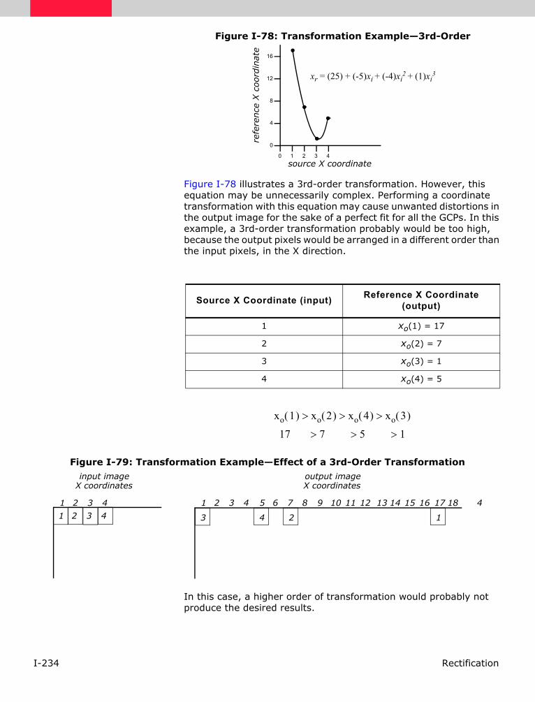
I-234 Rectification

Figure I-78: Transformation Example—3rd-Order

Figure I-78 illustrates a 3rd-order transformation. However, this equation may be unnecessarily complex. Performing a coordinate transformation with this equation may cause unwanted distortions in the output image for the sake of a perfect fit for all the GCPs. In this example, a 3rd-order transformation probably would be too high, because the output pixels would be arranged in a different order than the input pixels, in the X direction.

Figure I-79: Transformation Example—Effect of a 3rd-Order Transformation

In this case, a higher order of transformation would probably not produce the desired results.

Source X Coordinate (input) Reference X Coordinate (output)

1 xo(1) = 17

2 xo(2) = 7

3 xo(3) = 1

4 xo(4) = 5

0 1 2 3 4

0

4

8

12

16

refe

rence

X c

oord

inat

e

source X coordinate

xr = (25) + (-5)xi + (-4)xi2 + (1)xi

3

xo 1( ) xo 2( ) xo 4( ) xo 3( )> > >

17 7 5 1> > >

1 2 3 4 1 2 3 4 5 6 7 8 9 10 11 12 13 14 15 16 17 18 4

1 2 3 4 3 4 2 1

input imageX coordinates

output imageX coordinates

I-235Rectification

Minimum Number of GCPs Higher orders of transformation can be used to correct more complicated types of distortion. However, to use a higher order of transformation, more GCPs are needed. For instance, three points define a plane. Therefore, to perform a 1st-order transformation, which is expressed by the equation of a plane, at least three GCPs are needed. Similarly, the equation used in a 2nd-order transformation is the equation of a paraboloid. Six points are required to define a paraboloid. Therefore, at least six GCPs are required to perform a 2nd-order transformation. The minimum number of points required to perform a transformation of order t equals:

Use more than the minimum number of GCPs whenever possible. Although it is possible to get a perfect fit, it is rare, no matter how many GCPs are used.

For 1st- through 10th-order transformations, the minimum number of GCPs required to perform a transformation is listed in the following table:

For the best rectification results, you should always use more than the minimum number of GCPs, and they should be well-distributed.

Table I-45: Number of GCPs per Order of Transformation

Order of Transformation Minimum GCPs Required

1 3

2 6

3 10

4 15

5 21

6 28

7 36

8 45

9 55

10 66

t 1+( ) t 2+( )( )2

-------------------------------------

I-236 Rectification

Rubber Sheeting

Triangle-Based Finite Element Analysis

The finite element analysis is a powerful tool for solving complicated computation problems which can be approached by small simpler pieces. It has been widely used as a local interpolation technique in geographic applications. For image rectification, the known control points can be triangulated into many triangles. Each triangle has three control points as its vertices. Then, the polynomial transformation can be used to establish mathematical relationships between source and destination systems for each triangle. Because the transformation exactly passes through each control point and is not in a uniform manner, finite element analysis is also called rubber sheeting. It can also be called as the triangle-based rectification because the transformation and resampling for image rectification are performed on a triangle-by-triangle basis.

This triangle-based technique should be used when other rectification methods such as polynomial transformation and photogrammetric modeling cannot produce acceptable results.

Triangulation To perform the triangle-based rectification, it is necessary to triangulate the control points into a mesh of triangles. Watson ( Watson, 1992) summarily listed four kinds of triangulation, including the arbitrary, optimal, Greedy and Delaunay triangulation. Of the four kinds, the Delaunay triangulation is most widely used and is adopted because of the smaller angle variations of the resulting triangles.

The Delaunay triangulation can be constructed by the empty circumcircle criterion. The circumcircle formed from three points of any triangle does not have any other point inside. The triangles defined this way are the most equiangular possible.

Figure I-80 shows an example of the triangle network formed by 13 control points.

Figure I-80: Triangle Network

p0

p3

p8p10

p11

p4

p1

p12

p7p6

p2

p5

p9

I-237Rectification

Triangle-based rectification

Once the triangle mesh has been generated and the spatial order of the control points is available, the geometric rectification can be done on a triangle-by-triangle basis. This triangle-based method is appealing because it breaks the entire region into smaller subsets. If the geometric problem of the entire region is very complicated, the geometry of each subset can be much simpler and modeled through simple transformation.

For each triangle, the polynomials can be used as the general transformation form between source and destination systems.

Linear transformation The easiest and fastest is the linear transformation with the first order polynomials:

There is no need for extra information because there are three known conditions in each triangle and three unknown coefficients for each polynomial.

Nonlinear transformation Even though the linear transformation is easy and fast, it has one disadvantage. The transitions between triangles are not always smooth. This phenomenon is obvious when shaded relief or contour lines are derived from the DEM which is generated by the linear rubber sheeting. It is caused by incorporating the slope change of the control data at the triangle edges and vertices. In order to distribute the slope change smoothly across triangles, the nonlinear transformation with polynomial order larger than one is used by considering the gradient information.

The fifth order or quintic polynomial transformation is chosen here as the nonlinear rubber sheeting technique in this dissertation. It is a smooth function. The transformation function and its first order partial derivative are continuous. It is not difficult to construct ( Akima, 1978). The formula is as follows:

xo a0 a1x a2y+ +=

yo b0 b1x b2y+ +=

xo ak xi j– yj⋅ ⋅

j 0=

i

∑i 0=

5

∑=

yo bk xi j– yj⋅ ⋅

j 0=

i

∑i 0=

5

∑=

I-238 Rectification

It has 21 coefficients for each polynomial to be determined. For solving these unknowns, 21 conditions should be available. For each vertex of the triangle, one point value is given, and two first order and three second order partial derivatives can be easily derived by establishing a second order polynomial using vertices in the neighborhood of the vertex. Then the total 18 conditions are ready to be used. Three more conditions can be obtained by assuming that the normal partial derivative on each edge of the triangle is a cubic polynomial, which means that the sum of the polynomial items beyond the third order in the normal partial derivative has a value zero.

Check Point Analysis It should be emphasized that the independent check point analysis is critical for determining the accuracy of rubber sheeting modeling. For an exact modeling method like rubber sheeting, the ground control points, which are used in the modeling process, do not have much geometric residuals remaining. To evaluate the geometric transformation between source and destination coordinate systems, the accuracy assessment using independent check points is recommended.

RMS Error RMS error is the distance between the input (source) location of a GCP and the retransformed location for the same GCP. In other words, it is the difference between the desired output coordinate for a GCP and the actual output coordinate for the same point, when the point is transformed with the geometric transformation.

RMS error is calculated with a distance equation:

Where:

xi and yi are the input source coordinatesxr and yr are the retransformed coordinates

RMS error is expressed as a distance in the source coordinate system. If data file coordinates are the source coordinates, then the RMS error is a distance in pixel widths. For example, an RMS error of 2 means that the reference pixel is 2 pixels away from the retransformed pixel.

Residuals and RMS Error Per GCP

The GCP Tool contains columns for the X and Y residuals. Residuals are the distances between the source and retransformed coordinates in one direction. They are shown for each GCP. The X residual is the distance between the source X coordinate and the retransformed X coordinate. The Y residual is the distance between the source Y coordinate and the retransformed Y coordinate.

If the GCPs are consistently off in either the X or the Y direction, more points should be added in that direction. This is a common problem in off-nadir data.

RMS error xr xi–( )2 yr yi–( )2+=

I-239Rectification

RMS Error Per GCP

The RMS error of each point is reported to help you evaluate the GCPs. This is calculated with a distance formula:

Where:

Ri = the RMS error for GCPi

XRi = the X residual for GCPi

YRi = the Y residual for GCPi

Figure I-81 illustrates the relationship between the residuals and the RMS error per point.

Figure I-81: Residuals and RMS Error Per Point

Total RMS Error From the residuals, the following calculations are made to determine the total RMS error, the X RMS error, and the Y RMS error:

Where:

Rx = X RMS error

Ry = Y RMS error

T = total RMS error

n = the number of GCPs

i = GCP number

XRi = the X residual for GCPi

YRi = the Y residual for GCPi

Ri XRi2 YRi

2+=

source GCP

retransformed GCP

RMS error

X residual

Y residual

Rx1n--- XRi

2

i 1=

n

∑=

Ry1n--- YRi

2

i 1=

n

∑=

T Rx2 Ry

2+= or1n--- XRi

2 YRi2+

i 1=

n

∑

I-240 Rectification

Error Contribution by Point

A normalized value representing each point’s RMS error in relation to the total RMS error is also reported. This value is listed in the Contribution column of the GCP Tool.

Where:

Ei = error contribution of GCPi

Ri = the RMS error for GCPi

T = total RMS error

Tolerance of RMS Error In most cases, it is advantageous to tolerate a certain amount of error rather than take a more complex transformation. The amount of RMS error that is tolerated can be thought of as a window around each source coordinate, inside which a retransformed coordinate is considered to be correct (that is, close enough to use). For example, if the RMS error tolerance is 2, then the retransformed pixel can be 2 pixels away from the source pixel and still be considered accurate.

Figure I-82: RMS Error Tolerance

Acceptable RMS error is determined by the end use of the data base, the type of data being used, and the accuracy of the GCPs and ancillary data being used. For example, GCPs acquired from GPS should have an accuracy of about 10 m, but GCPs from 1:24,000-scale maps should have an accuracy of about 20 m.

It is important to remember that RMS error is reported in pixels. Therefore, if you are rectifying Landsat TM data and want the rectification to be accurate to within 30 meters, the RMS error should not exceed 1.00. Acceptable accuracy depends on the image area and the particular project.

Evaluating RMS Error To determine the order of polynomial transformation, you can assess the relative distortion in going from image to map or map to map. One should start with a 1st-order transformation unless it is known that it does not work. It is possible to repeatedly compute transformation matrices until an acceptable RMS error is reached.

EiRiT-----=

2 pixel RMS error tolerance(radius)

sourcepixel

Retransformed coordinateswithin this range are consideredcorrect

I-241Rectification

Most rectifications are either 1st-order or 2nd-order. The danger of using higher order rectifications is that the more complicated the equation for the transformation, the less regular and predictable the results are. To fit all of the GCPs, there may be very high distortion in the image.

After each computation of a transformation and RMS error, there are four options:

• Throw out the GCP with the highest RMS error, assuming that this GCP is the least accurate. Another transformation can then be computed from the remaining GCPs. A closer fit should be possible. However, if this is the only GCP in a particular region of the image, it may cause greater error to remove it.

• Tolerate a higher amount of RMS error.

• Increase the complexity of transformation, creating more complex geometric alterations in the image. A transformation can then be computed that can accommodate the GCPs with less error.

• Select only the points for which you have the most confidence.

Resampling Methods

The next step in the rectification/registration process is to create the output file. Since the grid of pixels in the source image rarely matches the grid for the reference image, the pixels are resampled so that new data file values for the output file can be calculated.

I-242 Rectification

Figure I-83: Resampling

The following resampling methods are supported in ERDAS IMAGINE:

• “Nearest Neighbor”—uses the value of the closest pixel to assign to the output pixel value.

• “Bilinear Interpolation”—uses the data file values of four pixels in a 2 × 2 window to calculate an output value with a bilinear function.

• “Cubic Convolution”—uses the data file values of sixteen pixels in a 4 × 4 window to calculate an output value with a cubic function.

• “Bicubic Spline Interpolation”—fits a cubic spline surface through the current block of points.

In all methods, the number of rows and columns of pixels in the output is calculated from the dimensions of the output map, which is determined by the geometric transformation and the cell size. The output corners (upper left and lower right) of the output file can be specified. The default values are calculated so that the entire source file is resampled to the destination file.

If an image to image rectification is being performed, it may be beneficial to specify the output corners relative to the reference file system, so that the images are coregistered. In this case, the upper left X and upper left Y coordinate are 0,0 and not the defaults.

If the output units are pixels, then the origin of the image is the upper left corner. Otherwise, the origin is the lower left corner.

1. The input image withsource GCPs.

2. The output grid, withreference GCPs shown.

3. To compare the two grids, theinput image is laid over theoutput grid, so that the GCPsof the two grids fit together.

4. Using a resampling method,the pixel values of the inputimage are assigned to pixelsin the output grid.

GCP

GCP

GCP

GCP

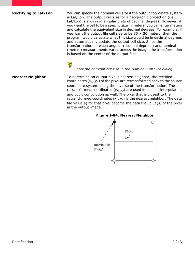
I-243Rectification

Rectifying to Lat/Lon You can specify the nominal cell size if the output coordinate system is Lat/Lon. The output cell size for a geographic projection (i.e., Lat/Lon) is always in angular units of decimal degrees. However, if you want the cell to be a specific size in meters, you can enter meters and calculate the equivalent size in decimal degrees. For example, if you want the output file cell size to be 30 × 30 meters, then the program would calculate what this size would be in decimal degrees and automatically update the output cell size. Since the transformation between angular (decimal degrees) and nominal (meters) measurements varies across the image, the transformation is based on the center of the output file.

Enter the nominal cell size in the Nominal Cell Size dialog.

Nearest Neighbor To determine an output pixel’s nearest neighbor, the rectified coordinates (xo, yo) of the pixel are retransformed back to the source coordinate system using the inverse of the transformation. The retransformed coordinates (xr, yr) are used in bilinear interpolation and cubic convolution as well. The pixel that is closest to the retransformed coordinates (xr, yr) is the nearest neighbor. The data file value(s) for that pixel become the data file value(s) of the pixel in the output image.

Figure I-84: Nearest Neighbor

(xr,yr)

nearest to(xr,yr)

I-244 Rectification

Bilinear Interpolation In bilinear interpolation, the data file value of the rectified pixel is based upon the distances between the retransformed coordinate location (xr, yr) and the four closest pixels in the input (source) image (see Figure I-85). In this example, the neighbor pixels are numbered 1, 2, 3, and 4. Given the data file values of these four pixels on a grid, the task is to calculate a data file value for r (Vr).

Table I-46: Nearest Neighbor Resampling

Advantages Disadvantages

Transfers original data values without averaging them as the other methods do; therefore, the extremes and subtleties of the data values are not lost. This is an important consideration when discriminating between vegetation types, locating an edge associated with a lineament, or determining different levels of turbidity or temperatures in a lake ( Jensen, 1996).

When this method is used to resample from a larger to a smaller grid size, there is usually a stair stepped effect around diagonal lines and curves.

Suitable for use before classification.

Data values may be dropped, while other values may be duplicated.

The easiest of the three methods to compute and the fastest to use.

Using on linear thematic data (e.g., roads, streams) may result in breaks or gaps in a network of linear data.

Appropriate for thematic files, which can have data file values based on a qualitative (nominal or ordinal) system or a quantitative (interval or ratio) system. The averaging that is performed with bilinear interpolation and cubic convolution is not suited to a qualitative class value system.

I-245Rectification

Figure I-85: Bilinear Interpolation

To calculate Vr, first Vm and Vn are considered. By interpolating Vm and Vn, you can perform linear interpolation, which is a simple process to illustrate. If the data file values are plotted in a graph relative to their distances from one another, then a visual linear interpolation is apparent. The data file value of m (Vm) is a function of the change in the data file value between pixels 3 and 1 (that is, V3 - V1).

Figure I-86: Linear Interpolation

The equation for calculating Vm from V1 and V3 is:

(xr,yr)

1 2

3 4

m r n

dy

dx

D

r is the location of the retransformed coordinate

V3

Vm

V1

(V3 - V1) / D

Y1 Ym Y3

Ddata file coordinates

dat

a file

val

ues

(Y)

Calculating a data file value as a functionof spatial distance between two pixels

VmV3 V1–

D------------------- dy V1+×=

I-246 Rectification

Where:

Yi = the Y coordinate for pixel i

Vi = the data file value for pixel i

dy = the distance between Y1 and Ym in the source coordinate system

D = the distance between Y1 and Y3 in the source coordinate system

If one considers that (V3 - V1 / D) is the slope of the line in the graph above, then this equation translates to the equation of a line in y = mx + b form.

Similarly, the equation for calculating the data file value for n (Vn) in the pixel grid is:

From Vn and Vm, the data file value for r, which is at the retransformed coordinate location (xr,yr),can be calculated in the same manner:

The following is attained by plugging in the equations for Vm and Vn to this final equation for Vr :

VnV4 V2–

D------------------- dy V2+×=

VrVn Vm–

D-------------------- dx Vm+×=

Vr

V4 V2–D

------------------- dy V2+×V3 V1–

D------------------- dy V1+×–

D------------------------------------------------------------------------------------------------------------ dx

V3 V1–D

------------------- dy V1+×+×=

VrV1 D dx–( ) D dy–( ) V2 dx( ) D dy–( ) V3 D dx–( ) dy( ) V4 dx( ) dy( )+ + +

D2--------------------------------------------------------------------------------------------------------------------------------------------------------------------------------=

I-247Rectification

In most cases D = 1, since data file coordinates are used as the source coordinates and data file coordinates increment by 1.

Some equations for bilinear interpolation express the output data file value as:

Where:

wi is a weighting factor

The equation above could be expressed in a similar format, in which the calculation of wi is apparent:

Where:

∆xi = the change in the X direction between (xr,yr) and the data file coordinate of pixel i

∆yi = the change in the Y direction between (xr,yr) and the data file coordinate of pixel i

Vi = the data file value for pixel i

D = the distance between pixels (in X or Y) in the source coordinate system

For each of the four pixels, the data file value is weighted more if the pixel is closer to (xr, yr).

Vr wiVi∑=

VrD xi∆–( ) D yi∆–( )

D2----------------------------------------------- Vi×

i 1=

4

∑=

I-248 Rectification

See "Enhancement" on page II-11 for more about convolution filtering.

Cubic Convolution Cubic convolution is similar to bilinear interpolation, except that:

• a set of 16 pixels, in a 4 × 4 array, are averaged to determine the output data file value, and

• an approximation of a cubic function, rather than a linear function, is applied to those 16 input values.

To identify the 16 pixels in relation to the retransformed coordinate (xr,yr), the pixel (i,j) is used, such that:

i = int (xr)j = int (yr)

This assumes that (xr,yr) is expressed in data file coordinates (pixels). The pixels around (i,j) make up a 4 × 4 grid of input pixels, as illustrated in Figure I-87.

Table I-47: Bilinear Interpolation Resampling

Advantages Disadvantages

Results in output images that are smoother, without the stair-stepped effect that is possible with nearest neighbor.

Since pixels are averaged, bilinear interpolation has the effect of a low-frequency convolution. Edges are smoothed, and some extremes of the data file values are lost.

More spatially accurate than nearest neighbor.

This method is often used when changing the cell size of the data, such as in SPOT/TM merges within the 2 × 2 resampling matrix limit.

I-249Rectification

Figure I-87: Cubic Convolution

Since a cubic, rather than a linear, function is used to weight the 16 input pixels, the pixels farther from (xr, yr) have exponentially less weight than those closer to (xr, yr).

Several versions of the cubic convolution equation are used in the field. Different equations have different effects upon the output data file values. Some convolutions may have more of the effect of a low-frequency filter (like bilinear interpolation), serving to average and smooth the values. Others may tend to sharpen the image, like a high-frequency filter. The cubic convolution used in ERDAS IMAGINE is a compromise between low-frequency and high-frequency. The general effect of the cubic convolution depends upon the data.

The formula used in ERDAS IMAGINE is:

(i,j)

(Xr,Yr)

Vr V i 1– j n 2–+,( ) f d i 1– j n 2–+,( ) 1+( )×

V i j n 2–+,( ) f d i j n 2–+,( )( )×

V i 1+ j n 2–+,( ) f d i 1+ j n 2–+,( ) 1–( )×

+

+

+

n 1=

4

∑=

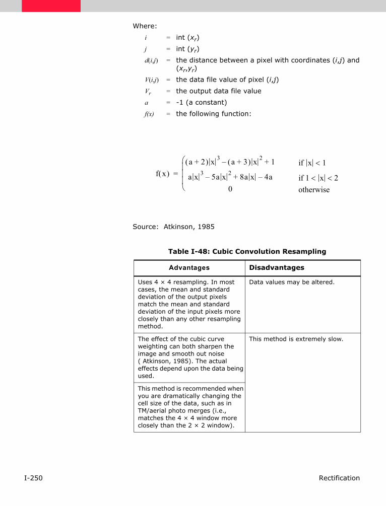
I-250 Rectification

Where:

i = int (xr)

j = int (yr)

d(i,j) = the distance between a pixel with coordinates (i,j) and (xr,yr)

V(i,j) = the data file value of pixel (i,j)

Vr = the output data file value

a = -1 (a constant)

f(x) = the following function:

Source: Atkinson, 1985

Table I-48: Cubic Convolution Resampling

Advantages Disadvantages

Uses 4 × 4 resampling. In most cases, the mean and standard deviation of the output pixels match the mean and standard deviation of the input pixels more closely than any other resampling method.

Data values may be altered.

The effect of the cubic curve weighting can both sharpen the image and smooth out noise ( Atkinson, 1985). The actual effects depend upon the data being used.

This method is extremely slow.

This method is recommended when you are dramatically changing the cell size of the data, such as in TM/aerial photo merges (i.e., matches the 4 × 4 window more closely than the 2 × 2 window).

f x( )a 2+( ) x 3 a 3+( ) x 2– 1+

a x 3 5a x 2– 8a x 4a–+0

=if x 1<

if 1 x 2< <otherwise

I-251Rectification

Bicubic Spline Interpolation

Bicubic Spline Interpolation is based on fitting a cubic spline surface through the current block of points. The output value is derived from the fitting surface that will retain the values of the known points. This algorithm is much slower than other methods of interpolation, but it has the advantage of giving a more exact fit to the curve without the oscillations that other interpolation methods can create. Bicubic Spline Interpolation is so similar to Bilinear Interpolation that unless you have the need to maximize surface smoothness, you should use Bilinear Interpolation.

Data Points

The known data points are an array of raster of m × n,

Where:

1 < i < m1 < j < nd is the cell size of the rasterVi,j is the cell value in (xi ,yj)

Equations

A bicubic polynomial function V(x,y) is constructed as following:

in each cell

x1 x2 xm-1 xm

y1

y2

yn-1

yn

V1,1 V2,1 Vm-1,1 Vm,1

V1,2

V1,n-1

V1,n

V2,2

V2,n-1

V2,n

Vm-1,2

Vm-1,n

Vm-1,n-1

Vm,2

Vm,n-1

Vm,n

Xi 1+ Xi d+=

Yj 1+ Yj d+=

Rij x y,( ) xi x xi 1+ yj y yj 1+ }≤ ≤,≤ ≤{=

I-252 Rectification

• The functions and their first and second derivatives must be continuous across the interval and equal at the endpoints and the fourth derivatives of the equations should be zero.

• The function satisfies the conditions

i.e., the spline must interpolate all data points.

• Coefficients can be obtained by resolving the known points together with the selection of the boundary condition type. Please refer to Shikin and Plis ( Shikin and Plis, 1995) for the boundary conditions and the mathematical details for solving the equations. IMAGINE uses the first type of boundary condition. Because in IMAGINE the input raster grid has been expanded two cells around the boundary, the boundary condition has no significant effects on the resampling.

Calculate value for unknown point

The value for point (xr, yr) can be calculated by the following formula:

V x y,( ) ap q,i j,( ) x xi–( )p y yj–( )q

q 0=

3

∑p 0=

3

∑=

i 1 2 … m j;, , , 1 2 … n, , ,= =

V xi yj,( ) Vi j, i; 1 2 … m j;, , , 1 2 … n, , ,= = =

V xr yr,( ) ap q,ir jr,( )

xr xir–( )p yr yjr

–( )q

q 0=

3

∑p 0=

3

∑=

I-253Rectification

The value is determined by 16 coefficients. Because the coefficients are resolved by using all other known points, all other points contribute to the value. The nearer points contribute more whereas the farther points contribute less.

Source: Shikin and Plis, 1995

Map-to-Map Coordinate Conversions

There are many instances when you may need to change a map that is already registered to a planar projection to another projection. Some examples of when this is required are as follows ( Environmental Systems Research Institute, 1992):

• When combining two maps with different projection characteristics.

• When the projection used for the files in the data base does not produce the desired properties of a map.

• When it is necessary to combine data from more than one zone of a projection, such as UTM or State Plane.

A change in the projection is a geometric change—distances, areas, and scale are represented differently. Therefore, the conversion process requires that pixels be resampled.

Table I-49: Bicubic Spline Interpolation

Advantages Disadvantages

Results in the smoothest output images.

The most computationally intensive resampling method, and is therefore the slowest.

More spatially accurate than nearest neighbor.

This method is often used when upsampling.

(ir, jr)

(xr ,yr)yjr

xir

d

d

I-254 Rectification

Resampling causes some of the spectral integrity of the data to be lost (see the disadvantages of the resampling methods explained previously). So, it is not usually wise to resample data that have already been resampled if the accuracy of data file values is important to the application. If the original unrectified data are available, it is usually wiser to rectify that data to a second map projection system than to lose a generation by converting rectified data and resampling it a second time.

Conversion Process To convert the map coordinate system of any georeferenced image, ERDAS IMAGINE provides a shortcut to the rectification process. In this procedure, GCPs are generated automatically along the intersections of a grid that you specify. The program calculates the reference coordinates for the GCPs with the appropriate conversion formula and a transformation that can be used in the regular rectification process.

Vector Data Converting the map coordinates of vector data is much easier than converting raster data. Since vector data are stored by the coordinates of nodes, each coordinate is simply converted using the appropriate conversion formula. There are no coordinates between nodes to extrapolate.

I-255Hardcopy Output

Hardcopy Output

Introduction Hardcopy output refers to any output of image data to paper. These topics are covered in this chapter:

• printing maps

• the mechanics of printing

For additional information, see the chapter about Windows printing in the ERDAS IMAGINE Configuration Guide.

Printing Maps ERDAS IMAGINE enables you to create and output a variety of types of hardcopy maps, with several referencing features.

Scaled Maps A scaled map is a georeferenced map that has been projected to a map projection, and is accurately laid-out and referenced to represent distances and locations. A scaled map usually has a legend, that includes a scale, such as 1 inch = 1000 feet. The scale is often expressed as a ratio, like 1:12,000, where 1 inch on the map represents 12,000 inches on the ground.

See "Rectification" on page I-219 for information on rectifying and georeferencing images and "Cartography" for information on creating maps.

Printing Large Maps Some scaled maps do not fit on the paper that is used by the printer. These methods are used to print and store large maps:

• A book map is laid out like the pages of a book. Each page fits on the paper used by the printer. There is a border, but no tick marks on every page.

• A paneled map is designed to be spliced together into a large paper map; therefore, borders and tick marks appear on the outer edges of the large map.

I-256 Hardcopy Output

Figure I-88: Layout for a Book Map and a Paneled Map

Scale and Resolution The following scales and resolutions are noticeable during the process of creating a map composition and sending the composition to a hardcopy device:

• spatial resolution of the image

• display scale of the map composition

• map scale of the image(s)

• map composition to paper scale

• device resolution

Spatial Resolution

Spatial resolution is the area on the ground represented by each raw image data pixel.

Display Scale

Display scale is the distance on the screen as related to one unit on paper. For example, if the map composition is 24 inches by 36 inches, it would not be possible to view the entire composition on the screen. Therefore, the scale could be set to 1:0.25 so that the entire map composition would be in view.

Map Scale

The map scale is the distance on a map as related to the true distance on the ground, or the area that one pixel represents measured in map units. The map scale is defined when you create an image area in the map composition. One map composition can have multiple image areas set at different scales. These areas may need to be shown at different scales for different applications.

neatline

map composition

neatline

map composition

++

++

++

++

tick marks

Book Map Paneled Map

I-257Hardcopy Output

Map Composition to Paper Scale

This scale is the original size of the map composition as related to the desired output size on paper.

Device Resolution

The number of dots that are printed per unit—for example, 300 dots per inch (DPI).

Use the ERDAS IMAGINE Map Composer to define the above scales and resolutions.

Map Scaling Examples The ERDAS IMAGINE Map Composer enables you to define a map size, as well as the size and scale for the image area within the map composition. The examples in this section focus on the relationship between these factors and the output file created by Map Composer for the specific hardcopy device or file format. Figure I-89 is the map composition that is used in the examples. This composition was originally created using the ERDAS IMAGINE Map Composer at a size of 22” × 34”, and the hardcopy output must be in two different formats.

• It must be output to a PostScript printer on an 8.5” × 11” piece of paper.

• A TIFF file must be created and sent to a film recorder having a 1,000 dpi resolution.

Figure I-89: Sample Map Composition

I-258 Hardcopy Output

Output to PostScript Printer

Since the map was created at 22” × 34”, the map composition to paper scale needs to be calculated so that the composition fits on an 8.5” × 11” piece of paper. If this scale is set for a one to one ratio, then the composition is paneled.

To determine the map composition to paper scale factor, it is necessary to calculate the most limiting direction. Since the printable area for the printer is approximately 8.1” × 8.6”, these numbers are used in the calculation.

• 8.1” / 22” = 0.36 (horizontal direction)

• 8.6” / 34” = 0.23 (vertical direction)

The vertical direction is the most limiting; therefore, the map composition to paper scale would be set for 0.23.

If the specified size of the map (width and height) is greater than the printable area for the printer, the output hardcopy map is paneled. See the hardware manual of the hardcopy device for information about the printable area of the device.

Use the Print Map Composition dialog to output a map composition to a PostScript printer.

Output to TIFF

The limiting factor in this example is not page size, but disk space (600 MB total). A three-band image file must be created in order to convert the map composition to .tif file. Due to the three bands and the high resolution, the image file could be very large. The .tif file is output to a film recorder with a 1,000 DPI device resolution.

To determine the number of megabytes for the map composition, the X and Y dimensions need to be calculated:

• X = 22 inches × 1,000 dots/inch = 22,000

• Y = 34 × 1,000 = 34,000

• 22,000 × 34,000 × 3 = 2244 MB (multiplied by 3 since there are 3 bands)

I-259Hardcopy Output

Although this appears to be an unmanageable file size, it is possible to reduce the file size with little image degradation. The image file created from the map composition must be less than half to accommodate the .tif file, because the total disk space is only 600 megabytes. Dividing the map composition by three in both X and Y directions (2,244 MB / 3 /3) results in approximately a 250 megabyte file. This file size is small enough to process and leaves enough room for the image to TIFF conversion. This division is accomplished by specifying a 1/3 or 0.333 map composition to paper scale when outputting the map composition to an image file.

Once the image file is created and exported to TIFF format, it can be sent to a film recorder that accepts .tif files. Remember, the file must be enlarged three times to compensate for the reduction during the image file creation.

See the hardware manual of the hardcopy device for information about the DPI device resolution.

Use the ERDAS IMAGINE Print Map Composition dialog to output a map composition to an image file.

Mechanics of Printing

This section describes the mechanics of transferring an image or map composition from a data file to a hardcopy map.

Halftone Printing Halftoning is the process of converting a continuous tone image into a pattern of dots. A newspaper photograph is a common example of halftoning.

To make a color illustration, halftones in the primary colors (cyan, magenta, and yellow), plus black, are overlaid. The halftone dots of different colors, in close proximity, create the effect of blended colors in much the same way that phosphorescent dots on a color computer monitor combine red, green, and blue to create other colors. By using different patterns of dots, colors can have different intensities. The dots for halftoning are a fixed density—either a dot is there or it is not there.

For scaled maps, each output pixel may contain one or more dot patterns. If a very large image file is being printed onto a small piece of paper, data file pixels are skipped to accommodate the reduction.

Hardcopy Devices

The following hardcopy devices use halftoning to output an image or map composition:

• Tektronix Inkjet Printer

• Tektronix Phaser Printer

I-260 Hardcopy Output

See the user’s manual for the hardcopy device for more information about halftone printing.

Continuous Tone Printing Continuous tone printing enables you to output color imagery using the four process colors (cyan, magenta, yellow, and black). By using varying percentages of these colors, it is possible to create a wide range of colors. The printer converts digital data from the host computer into a continuous tone image. The quality of the output picture is similar to a photograph. The output is smoother than halftoning because the dots for continuous tone printing can vary in density.

Example

There are different processes by which continuous tone printers generate a map. One example is a process called thermal dye transfer. The entire image or map composition is loaded into the printer’s memory. While the paper moves through the printer, heat is used to transfer the dye from a ribbon, which has the dyes for all of the four process colors, to the paper. The density of the dot depends on the amount of heat applied by the printer to transfer the dye. The amount of heat applied is determined by the brightness values of the input image. This allows the printer to control the amount of dye that is transferred to the paper to create a continuous tone image.

Hardcopy Devices

The following hardcopy device uses continuous toning to output an image or map composition:

• Tektronix Phaser II SD

NOTE: The above printers do not necessarily use the thermal dye transfer process to generate a map.

See the user’s manual for the hardcopy device for more information about continuous tone printing.

Contrast and Color Tables ERDAS IMAGINE contrast and color tables are used for some printing processes, just as they are used in displaying an image. For continuous raster layers, they are loaded from the ERDAS IMAGINE contrast table. For thematic layers, they are loaded from the color table. The translation of data file values to brightness values is performed entirely by the software program.

I-261Hardcopy Output

RGB to CMY Conversion

Colors

Since a printer uses ink instead of light to create a visual image, the primary colors of pigment (cyan, magenta, and yellow) are used in printing, instead of the primary colors of light (red, green, and blue). Cyan, magenta, and yellow can be combined to make black through a subtractive process, whereas the primary colors of light are additive—red, green, and blue combine to make white ( Gonzalez and Wintz, 1977).

The data file values that are sent to the printer and the contrast and color tables that accompany the data file are all in the RGB color scheme. The RGB brightness values in the contrast and color tables must be converted to cyan, magenta, and yellow (CMY) values.

The RGB primary colors are the opposites of the CMY colors—meaning, for example, that the presence of cyan in a color means an equal lack of red. To convert the values, each RGB brightness value is subtracted from the maximum brightness value to produce the brightness value for the opposite color. The following equation shows this relationship:

C = MAX - R

M = MAX - G

Y = MAX - B

Where:

MAX = the maximum brightness value

R = red value from lookup table

G = green value from lookup table

B = blue value from lookup table

C = calculated cyan value

M = calculated magenta value

Y = calculated yellow value

Black Ink

Although, theoretically, cyan, magenta, and yellow combine to create black ink, the color that results is often a dark, muddy brown. Many printers also use black ink for a truer black.

NOTE: Black ink may not be available on all printers. Consult the user’s manual for your printer.

Images often appear darker when printed than they do when displayed on the display device. Therefore, it may be beneficial to improve the contrast and brightness of an image before it is printed.

Use the programs discussed in "Enhancement" on page II-11 to brighten or enhance an image before it is printed.

I-262 Hardcopy Output

I-263Map Projections

Map Projections

Introduction This appendix is an alphabetical listing of the map projections supported in ERDAS IMAGINE. It is divided into two sections:

• USGS Projections, and

• External Projections

The external projections were implemented outside of ERDAS IMAGINE so that you could add to these using the IMAGINE Developers’ Toolkit. The projections in each section are presented in alphabetical order.

The information in this appendix is adapted from:

• Map Projections for Use with the Geographic Information System ( Lee and Walsh, 1984)

• Map Projections—A Working Manual ( Snyder, 1987)

• ArcInfo HELP ( Environmental Systems Research Institute, 1997)

Other sources are noted in the text.

For general information about map projection types, refer to "Cartography" on page I-183.

Rectify an image to a particular map projection using the ERDAS IMAGINE Rectification tools. View, add, or change projection information using the Image Information option.

NOTE: You cannot rectify to a new map projection using the Image Information option. You should change map projection information using Image Information only if you know the information to be incorrect. Use the rectification tools to actually georeference an image to a new map projection system.

I-264 Map Projections

USGS Projections The following USGS map projections are supported in ERDAS IMAGINE and are described in this section:

• Alaska Conformal

• Albers Conical Equal Area

• Azimuthal Equidistant

• Behrmann

• Bonne

• Cassini

• Eckert I

• Eckert II

• Eckert III

• Eckert IV

• Eckert V

• Eckert VI

• EOSAT SOM

• Equidistant Conic

• Equidistant Cylindrical

• Equirectangular (Plate Carrée)

• Gall Stereographic

• Gauss Kruger

• General Vertical Near-side Perspective

• Geographic (Lat/Lon)

• Gnomonic

• Hammer

• Interrupted Goode Homolosine

• Interrupted Mollweide

• Lambert Azimuthal Equal Area

• Lambert Conformal Conic

I-265Map Projections

• Loximuthal

• Mercator

• Miller Cylindrical

• Modified Transverse Mercator

• Mollweide

• New Zealand Map Grid

• Oblated Equal Area

• Oblique Mercator (Hotine)

• Orthographic

• Plate Carrée

• Polar Stereographic

• Polyconic

• Quartic Authalic

• Robinson

• RSO

• Sinusoidal

• Space Oblique Mercator

• Space Oblique Mercator (Formats A & B)

• State Plane

• Stereographic

• Stereographic (Extended)

• Transverse Mercator

• Two Point Equidistant

• UTM

• Van der Grinten I

• Wagner IV

• Wagner VII

I-266 Map Projections

• Winkel I

I-267Map Projections

Alaska Conformal Use of this projection results in a conformal map of Alaska. It has little scale distortion as compared to other conformal projections. The method of projection is “modified planar. [It is] a sixth-order-equation modification of an oblique Stereographic conformal projection on the Clarke 1866 spheroid. The origin is at 64° N, 152° W” ( Environmental Systems Research Institute, 1997).

Source: Environmental Systems Research Institute, 1997

PromptsThe following prompts display in the Projection Chooser once Alaska Conformal is selected. Respond to the prompts as described.

Spheroid Name

Datum Name

Select the spheroid and datum to use.

The list of available spheroids is located in Table I-44 on page I-214.

False easting

False northing

Table I-50: Alaska Conformal Summary

Construction Modified planar

Property Conformal

Meridians N/A

Parallels N/A

Graticule spacing

N/A

Linear scale

The minimum scale factor is 0.997 at roughly 62.5° N, 156° W. Scale increases outward from these coordinates. Most of Alaska and the Aleutian Islands (with the exception of the panhandle) is bounded by a line of true scale. The scale factor for Alaska is from 0.997 to 1.003. That is one quarter the range for a corresponding conic projection ( Snyder, 1987).

Uses

This projection is useful for mapping the complete state of Alaska on the Clarke 1866 spheroid or NAD27, but not with other datums and spheroids. Distortion increases as distance from Alaska increases.

I-268 Map Projections

Enter values of false easting and false northing corresponding to the desired center of the projection. These values must be in meters. It is often convenient to make them large enough so that no negative coordinates occur within the region of the map projection. That is, the origin of the rectangular coordinate system should fall outside of the map projection to the south and west.

I-269Map Projections

Albers Conical Equal Area

The Albers Conical Equal Area projection is mathematically based on a cone that is conceptually secant on two parallels. There is no areal deformation. The North or South Pole is represented by an arc. It retains its properties at various scales, and individual sheets can be joined along their edges.

This projection produces very accurate area and distance measurements in the middle latitudes (Figure I-90). Thus, Albers Conical Equal Area is well-suited to countries or continents where north-south depth is about 3/5 the breadth of east-west. When this projection is used for the continental US, the two standard parallels are 29.5° and 45.5° North.

This projection possesses the property of equal-area, and the standard parallels are correct in scale and in every direction. Thus, there is no angular distortion (i.e., meridians intersect parallels at right angles), and conformality exists along the standard parallels. Like other conics, Albers Conical Equal Area has concentric arcs for parallels and equally spaced radii for meridians. Parallels are not equally spaced, but are farthest apart between the standard parallels and closer together on the north and south edges.

Table I-51: Albers Conical Equal Area Summary

Construction Cone

Property Equal-area

Meridians Meridians are straight lines converging on the polar axis, but not at the pole.

Parallels Parallels are arcs of concentric circles concave toward a pole.

Graticule spacing

Meridian spacing is equal on the standard parallels and decreases toward the poles. Parallel spacing decreases away from the standard parallels and increases between them. Meridians and parallels intersect each other at right angles. The graticule spacing preserves the property of equivalence of area. The graticule is symmetrical.

Linear scale

Linear scale is true on the standard parallels. Maximum scale error is 1.25% on a map of the United States (48 states) with standard parallels of 29.5°N and 45.5°N.

Uses

Used for thematic maps. Used for large countries with an east-west orientation. Maps based on the Albers Conical Equal Area for Alaska use standard parallels 55°N and 65°N; for Hawaii, the standard parallels are 8°N and 18°N. The National Atlas of the United States, United States Base Map (48 states), and the Geologic map of the United States are based on the standard parallels of 29.5°N and 45.5°N.

I-270 Map Projections

Albers Conical Equal Area is the projection exclusively used by the USGS for sectional maps of all 50 states of the US in the National Atlas of 1970.

PromptsThe following prompts display in the Projection Chooser once Albers Conical Equal Area is selected. Respond to the prompts as described.

Spheroid Name

Datum Name

Select the spheroid and datum to use.

The list of available spheroids is located in Table I-44 on page I-214.

Latitude of 1st standard parallel

Latitude of 2nd standard parallel

Enter two values for the desired control lines of the projection (i.e., the standard parallels). Note that the first standard parallel is the southernmost.

Then, define the origin of the map projection in both spherical and rectangular coordinates.

Longitude of central meridian

Latitude of origin of projection

Enter values for longitude of the desired central meridian and latitude of the origin of projection.

False easting at central meridian

False northing at origin

Enter values of false easting and false northing, corresponding to the intersection of the central meridian and the latitude of the origin of projection. These values must be in meters. It is often convenient to make them large enough to prevent negative coordinates from occurring within the region of the map projection. That is, the origin of the rectangular coordinate system should fall outside of the map projection to the south and west.

I-271Map Projections

Figure I-90: Albers Conical Equal Area Projection

In Figure I-90, the standard parallels are 20°N and 60°N. Note the change in spacing of the parallels.

I-272 Map Projections

Azimuthal Equidistant

The Azimuthal Equidistant projection is mathematically based on a plane tangent to the Earth. The entire Earth can be represented, but generally less than one hemisphere is portrayed, though the other hemisphere can be portrayed, but is much distorted. It has true direction and true distance scaling from the point of tangency.

Table I-52: Azimuthal Equidistant Summary

Construction Plane

Property Equidistant

Meridians

Polar aspect: the meridians are straight lines radiating from the point of tangency.

Oblique aspect: the meridians are complex curves concave toward the point of tangency.

Equatorial aspect: the meridians are complex curves concave toward a straight central meridian, except the outer meridian of a hemisphere, which is a circle.

Parallels

Polar aspect: the parallels are concentric circles.

Oblique aspect: the parallels are complex curves.

Equatorial aspect: the parallels are complex curves concave toward the nearest pole; the Equator is straight.

Graticule spacing

Polar aspect: the meridian spacing is equal and increases away from the point of tangency. Parallel spacing is equidistant. Angular and area deformation increase away from the point of tangency.

Linear scale

Polar aspect: linear scale is true from the point of tangency along the meridians only.

Oblique and equatorial aspects: linear scale is true from the point of tangency. In all aspects, the projection shows distances true to scale when measured between the point of tangency and any other point on the map.

Uses

The Azimuthal Equidistant projection is used for radio and seismic work, as every place in the world is shown at its true distance and direction from the point of tangency. The USGS uses the oblique aspect in the National Atlas and for large-scale mapping of Micronesia. The polar aspect is used as the emblem of the United Nations.

I-273Map Projections

This projection is used mostly for polar projections because latitude rings divide meridians at equal intervals with a polar aspect (Figure I-91). Linear scale distortion is moderate and increases toward the periphery. Meridians are equally spaced, and all distances and directions are shown accurately from the central point.

This projection can also be used to center on any point on the Earth (e.g., a city) and distance measurements are true from that central point. Distances are not correct or true along parallels, and the projection is neither equal-area nor conformal. Also, straight lines radiating from the center of this projection represent great circles.

PromptsThe following prompts display in the Projection Chooser if Azimuthal Equidistant is selected. Respond to the prompts as described.

Spheroid Name

Datum Name

Select the spheroid and datum to use.

The list of available spheroids is located in Table I-44 on page I-214.

Define the center of the map projection in both spherical and rectangular coordinates.

Longitude of center of projection

Latitude of center of projection

Enter values for the longitude and latitude of the desired center of the projection.

False easting

False northing

Enter values of false easting and false northing corresponding to the center of the projection. These values must be in meters. It is often convenient to make them large enough so that no negative coordinates occur within the region of the map projection. That is, the origin of the rectangular coordinate system should fall outside of the map projection to the south and west.

I-274 Map Projections

Figure I-91: Polar Aspect of the Azimuthal Equidistant Projection

This projection is commonly used in atlases for polar maps.

I-275Map Projections

Behrmann With the exception of compression in the horizontal direction and expansion in the vertical direction, the Behrmann projection is the same as the Lambert Cylindrical Equal-area projection. These changes prevent distortion at latitudes 30° N and S instead of at the Equator.

Source: Snyder and Voxland, 1989

PromptsThe following prompts display in the Projection Chooser once Behrmann is selected. Respond to the prompts as described.

Spheroid Name

Datum Name

Select the spheroid and datum to use.

The list of available spheroids is located in Table I-44 on page I-214.

Longitude of central meridian

Enter a value of the longitude of the desired central meridian.

False easting

False northing

Enter values of false easting and false northing corresponding to the desired center of the projection. These values must be in meters. It is often convenient to make them large enough so that no negative coordinates occur within the region of the map projection. That is, the origin of the rectangular coordinate system should fall outside of the map projection to the south and west.

Table I-53: Behrmann Summary

Construction Cylindrical

Property Equal-area

Meridians Straight parallel lines that are equally spaced and 0.42 the length of the Equator.

Parallels Straight lines that are unequally spaced and farthest apart near the Equator, perpendicular to meridians.

Graticule spacing See Meridians and Parallels. Poles are straight lines the same length as the Equator. Symmetry is present about any meridian or the Equator.

Linear scale Scale is true along latitudes 30° N and S.

Uses Used for creating world maps.

I-276 Map Projections

Figure I-92: Behrmann Cylindrical Equal-Area Projection

Source: Snyder and Voxland, 1989

I-277Map Projections

Bonne The Bonne projection is an equal-area projection. True scale is achievable along the central meridian and all parallels. Although it was used in the 1800s and early 1900s, Bonne was replaced by Lambert Azimuthal Equal Area by the mapping company Rand McNally & Co. and Hammond, Inc. (see "Lambert Azimuthal Equal Area" on page I-312)

Source: Environmental Systems Research Institute, 1997

PromptsThe following prompts display in the Projection Chooser once Bonne is selected. Respond to the prompts as described.

Spheroid Name

Datum Name

Select the spheroid and datum to use.

The list of available spheroids is located in Table I-44 on page I-214.

Latitude of standard parallel

Longitude of central meridian

Enter values of the latitude of standard parallel and the longitude of central meridian.

False easting

False northing

Table I-54: Bonne Summary

Construction Pseudocone

Property Equal-area

Meridians N/A

Parallels Parallels are concentric arcs that are equally spaced.

Graticule spacing

The central meridian is a linear graticule.

Linear scale Scale is true along the central meridian and all parallels.

Uses This projection is best used on maps of continents and small areas. There is some distortion.

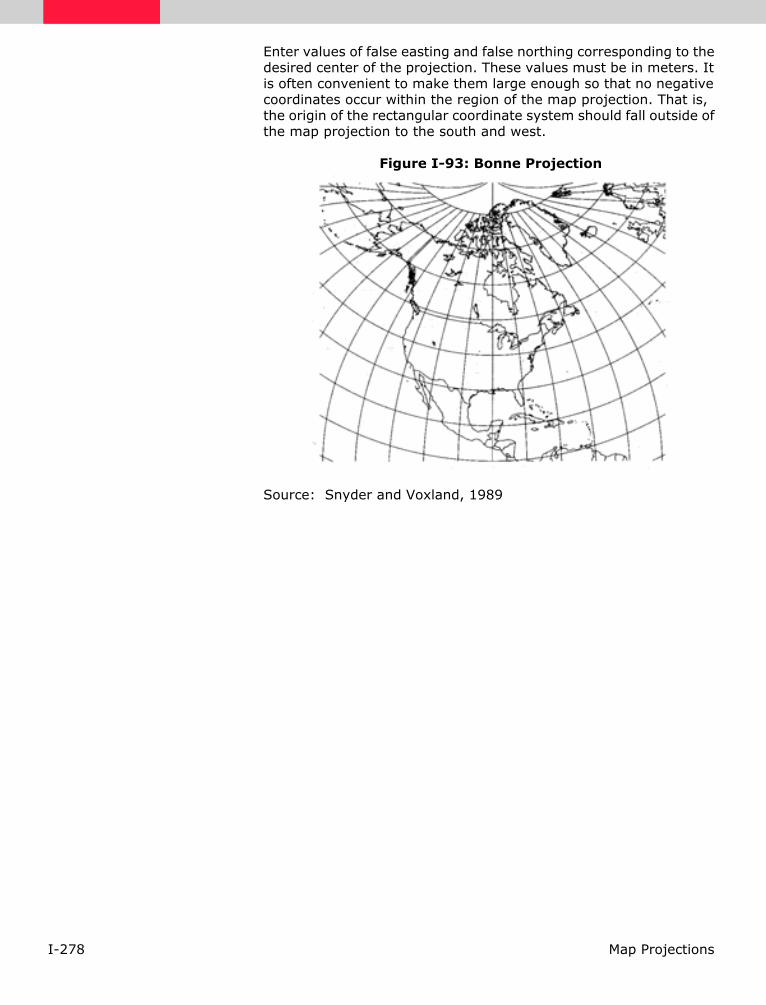
I-278 Map Projections

Enter values of false easting and false northing corresponding to the desired center of the projection. These values must be in meters. It is often convenient to make them large enough so that no negative coordinates occur within the region of the map projection. That is, the origin of the rectangular coordinate system should fall outside of the map projection to the south and west.

Figure I-93: Bonne Projection

Source: Snyder and Voxland, 1989

I-279Map Projections

Cassini The Cassini projection is a transverse cylindrical projection and is neither equal-area or conformal. It is best used for areas that are mostly in the north-south direction.

Source: Environmental Systems Research Institute, 1997

PromptsThe following prompts display in the Projection Chooser once Cassini is selected. Respond to the prompts as described.

Spheroid Name

Datum Name

Select the spheroid and datum to use.

The list of available spheroids is located in Table I-44 on page I-214.

Scale Factor

Enter the scale factor.

Longitude of central meridian

Latitude of origin of projection

Enter the values for longitude of central meridian and latitude of origin of projection.

False easting

False northing

Table I-55: Cassini Summary

Construction Cylinder

Property Compromise

Meridians N/A

Parallels N/A

Graticule spacing

Linear graticules are located at the Equator, central meridian, as well as meridians 90° from the central meridian.

Linear scale

With increasing distance from central meridian, scale distortion increases. Scale is true along the central meridian and lines perpendicular to the central meridian.

UsesCassini is used for large maps of areas near the central meridian. The extent is 5 degrees to either side of the central meridian.

I-280 Map Projections

Enter values of false easting and false northing corresponding to the desired center of the projection. These values must be in meters. It is often convenient to make them large enough so that no negative coordinates occur within the region of the map projection. That is, the origin of the rectangular coordinate system should fall outside of the map projection to the south and west.

Figure I-94: Cassini Projection

Source: Snyder and Voxland, 1989

I-281Map Projections

Eckert I A great amount of distortion at the Equator is due to the break at the Equator.

Source: Snyder and Voxland, 1989

Prompts The following prompts display in the Projection Chooser once Eckert I is selected. Respond to the prompts as described.

Spheroid Name

Datum Name

Select the spheroid and datum to use.

The list of available spheroids is located in Table I-44 on page I-214.

Longitude of central meridian

Enter a value of the longitude of the desired central meridian.

False easting

False northing

Enter values of false easting and false northing corresponding to the desired center of the projection. These values must be in meters. It is often convenient to make them large enough so that no negative coordinates occur within the region of the map projection. That is, the origin of the rectangular coordinate system should fall outside of the map projection to the south and west.

Table I-56: Eckert I Summary

Construction Pseudocylinder

Property Neither conformal nor equal-area

Meridians Meridians are converging straight lines that are equally spaced and broken at the Equator.

Parallels Parallels are perpendicular to the central meridian, equally spaced straight parallel lines.

Graticule spacing See Meridians and Parallels. Poles are lines one half the length of the Equator. Symmetry exists about the central meridian or the Equator.

Linear scale Scale is true along latitudes 47° 10’ N and S. Scale is constant at any latitude (and latitude of opposite sign) and any meridian.

Uses This projection is used as a novelty to show a straight-line graticule.

I-282 Map Projections

Figure I-95: Eckert I Projection

Source: Snyder and Voxland, 1989

I-283Map Projections

Eckert II The break at the Equator creates a great amount of distortion there. Eckert II is similar to the Eckert I projection. The Eckert I projection has meridians positioned identically to Eckert II, but the Eckert I projection has equidistant parallels.

Source: Snyder and Voxland, 1989

Prompts The following prompts display in the Projection Chooser once Eckert II is selected. Respond to the prompts as described.

Spheroid Name

Datum Name

Select the spheroid and datum to use.

The list of available spheroids is located in Table I-44 on page I-214.

Longitude of central meridian

Enter a value of the longitude of the desired central meridian.

False easting

False northing

Enter values of false easting and false northing corresponding to the desired center of the projection. These values must be in meters. It is often convenient to make them large enough so that no negative coordinates occur within the region of the map projection. That is, the origin of the rectangular coordinate system should fall outside of the map projection to the south and west.

Table I-57: Eckert II Summary

Construction Pseudocylinder

Property Equal-area

Meridians Meridians are straight lines that are equally spaced and broken at the Equator. Central meridian is one half as long as the Equator.

Parallels Parallels are straight parallel lines that are unequally spaced. The greatest separation is close to the Equator. Parallels are perpendicular to the central meridian.

Graticule spacing See Meridians and Parallels. Pole lines are half the length of the Equator. Symmetry exists at the central meridian or the Equator.

Linear scale Scale is true along altitudes 55° 10’ N, and S. Scale is constant along any latitude.

Uses This projection is used as a novelty to show straight-line equal-area graticule.

I-284 Map Projections

Figure I-96: Eckert II Projection

Source: Snyder and Voxland, 1989

I-285Map Projections

Eckert III In the Eckert III projection, “no point is free of all scale distortion, but the Equator is free of angular distortion” ( Snyder and Voxland, 1989).

Source: Environmental Systems Research Institute, 1997

PromptsThe following prompts display in the Projection Chooser once Eckert III is selected. Respond to the prompts as described.

Spheroid Name

Datum Name

Select the spheroid and datum to use.

The list of available spheroids is located in Table I-44 on page I-214.

Longitude of central meridian

Enter a value of the longitude of the desired central meridian.

False easting

False northing

Enter values of false easting and false northing corresponding to the desired center of the projection. These values must be in meters. It is often convenient to make them large enough so that no negative coordinates occur within the region of the map projection. That is, the origin of the rectangular coordinate system should fall outside of the map projection to the south and west.

Table I-58: Eckert III Summary

Construction Pseudocylinder

Property Area is not preserved.

Meridians Meridians are elliptical curves that are equally spaced elliptical curves. The meridians +/- 180° from the central meridian are semicircles. The poles and the central meridian are straight lines one half the length of the Equator.

Parallels Parallels are equally spaced straight lines.

Graticule spacing See Meridians and Parallels. Pole lines are half the length of the Equator. Symmetry exists at the central meridian or the Equator.

Linear scale Scale is correct only along 37° and 55’ N and S. Features close to poles are compressed in the north-south direction.

Uses Used for mapping the world.

I-286 Map Projections

Figure I-97: Eckert III Projection

Source: Snyder and Voxland, 1989

I-287Map Projections

Eckert IV The Eckert IV projection is best used for thematic maps of the globe. An example of a thematic map is one depicting land cover.

Source: Environmental Systems Research Institute, 1997

PromptsThe following prompts display in the Projection Chooser once Eckert IV is selected. Respond to the prompts as described.

Spheroid Name

Datum Name

Select the spheroid and datum to use.

The list of available spheroids is located in Table I-44 on page I-214.

Longitude of central meridian

Enter a value of the longitude of the desired central meridian.

False easting

False northing

Enter values of false easting and false northing corresponding to the desired center of the projection. These values must be in meters. It is often convenient to make them large enough so that no negative coordinates occur within the region of the map projection. That is, the origin of the rectangular coordinate system should fall outside of the map projection to the south and west.

Table I-59: Eckert IV Summary

Construction Pseudocylinder

Property Equal-area

Meridians Meridians are elliptical arcs that are equally spaced.

Parallels Parallels are straight lines that are unequally spaced and closer together at the poles.

Graticule spacing

See Meridians and Parallels. The poles and the central meridian are straight lines one half the length of the Equator.

Linear scale

“Scale is distorted north-south 40 percent along the Equator relative to the east-west dimension. This distortion decreases to zero at 40° 30’ N and S and at the central meridian. Scale is correct only along these parallels. Nearer the poles, features are compressed in the north-south direction” ( Environmental Systems Research Institute, 1997).

Uses Use for world maps only.

I-288 Map Projections

Figure I-98: Eckert IV Projection

Source: Snyder and Voxland, 1989

I-289Map Projections

Eckert V The Eckert V projection is only supported on a sphere. Like Eckert III, no point is free of all scale distortion, but the Equator is free of angular distortion” ( Snyder and Voxland, 1989).

Source: Environmental Systems Research Institute, 1997

PromptsThe following prompts display in the Projection Chooser once Eckert V is selected. Respond to the prompts as described.

Spheroid Name

Datum Name

Select the spheroid and datum to use.

The list of available spheroids is located in Table I-44 on page I-214.

Longitude of central meridian

Enter a value of the longitude of the desired central meridian.

False easting

False northing

Enter values of false easting and false northing corresponding to the desired center of the projection. These values must be in meters. It is often convenient to make them large enough so that no negative coordinates occur within the region of the map projection. That is, the origin of the rectangular coordinate system should fall outside of the map projection to the south and west.

Figure I-99: Eckert V Summary

Construction Pseudocylinder

Property Area is not preserved.

Meridians Meridians are sinusoidal curves that are equally spaced. The poles and the central meridian are straight lines one half as long as the Equator.

Parallels Parallels are straight lines that are equally spaced.

Graticule spacing See Meridians and Parallels.

Linear scale Scale is correct only along 37° 55’ N and S. Features near the poles are compressed in the north-south direction.

Uses This projection is best used for thematic world maps.

I-290 Map Projections

Figure I-100: Eckert V Projection

Source: Snyder and Voxland, 1989

I-291Map Projections

Eckert VI The Eckert VI projection is best used for thematic maps. An example of a thematic map is one depicting land cover.

Source: Environmental Systems Research Institute, 1997

PromptsThe following prompts display in the Projection Chooser once Eckert VI is selected. Respond to the prompts as described.

Spheroid Name

Datum Name

Select the spheroid and datum to use.

The list of available spheroids is located in Table I-44 on page I-214.

Longitude of central meridian

Enter a value of the longitude of the desired central meridian.

False easting

False northing

Enter values of false easting and false northing corresponding to the desired center of the projection. These values must be in meters. It is often convenient to make them large enough so that no negative coordinates occur within the region of the map projection. That is, the origin of the rectangular coordinate system should fall outside of the map projection to the south and west.

Table I-60: Eckert VI Summary

Construction Pseudocylinder

Property Equal-area

Meridians Meridians are sinusoidal curves that are equally spaced.

Parallels Parallels are unequally spaced straight lines, closer together at the poles.

Graticule spacing

See Meridians and Parallels. The poles and the central meridian are straight lines one half the length of the Equator.

Linear scale

“Scale is distorted north-south 29 percent along the Equator relative to the east-west dimension. This distortion decreases to zero at 49° 16’ N and S at the central meridian. Scale is correct only along these parallels. Nearer the poles, features are compressed in the north-south direction” ( Environmental Systems Research Institute, 1997).

Uses Use for world maps only.

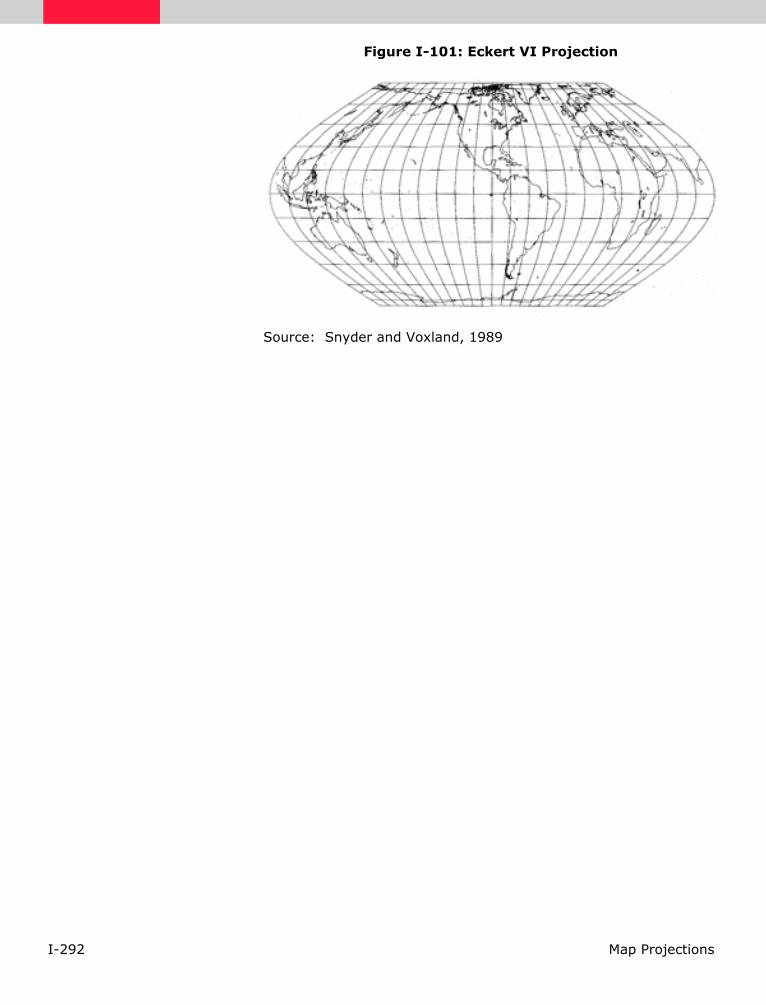
I-292 Map Projections

Figure I-101: Eckert VI Projection

Source: Snyder and Voxland, 1989

I-293Map Projections

EOSAT SOM The EOSAT SOM projection is similar to the Space Oblique Mercator projection. The main exception to the similarity is that the EOSAT SOM projection’s X and Y coordinates are switched.

For information, see "Space Oblique Mercator" on page I-350.

PromptsThe following prompts display in the Projection Chooser once EOSAT SOM is selected. Respond to the prompts as described.

Spheroid Name

Datum Name

Select the spheroid and datum to use.

The list of available spheroids is located in Table I-44 on page I-214.

Landsat vehicle ID (1-5)

Specify whether the data are from Landsat 1, 2, 3, 4, or 5.

Orbital path number (1-251 or 1-233)

For Landsats 1, 2, and 3, the path range is from 1 to 251. For Landsats 4 and 5, the path range is from 1 to 233.

False easting

False northing

Enter values of false easting and false northing corresponding to the desired center of the projection. These values must be in meters. It is often convenient to make them large enough so that no negative coordinates occur within the region of the map projection. That is, the origin of the rectangular coordinate system should fall outside of the map projection to the south and west.

I-294 Map Projections

Equidistant Conic With Equidistant Conic (Simple Conic) projections, correct distance is achieved along the line(s) of contact with the cone, and parallels are equidistantly spaced. It can be used with either one (A) or two (B) standard parallels.

This projection is neither conformal nor equal-area, but the north-south scale along meridians is correct. The North or South Pole is represented by an arc. Because scale distortion increases with increasing distance from the line(s) of contact, the Equidistant Conic is used mostly for mapping regions predominantly east-west in extent. The USGS uses the Equidistant Conic in an approximate form for a map of Alaska.

PromptsThe following prompts display in the Projection Chooser if Equidistant Conic is selected. Respond to the prompts as described.

Spheroid Name

Datum Name

Select the spheroid and datum to use.

The list of available spheroids is located in Table I-44 on page I-214.

Table I-61: Equidistant Conic Summary

Construction Cone

Property Equidistant

Meridians Meridians are straight lines converging on a polar axis but not at the pole.

Parallels Parallels are arcs of concentric circles concave toward a pole.

Graticule spacing

Meridian spacing is true on the standard parallels and decreases toward the pole. Parallels are placed at true scale along the meridians. Meridians and parallels intersect each other at right angles. The graticule is symmetrical.

Linear scale Linear scale is true along all meridians and along the standard parallel or parallels.

Uses

The Equidistant Conic projection is used in atlases for portraying mid-latitude areas. It is good for representing regions with a few degrees of latitude lying on one side of the Equator. It was used in the former Soviet Union for mapping the entire country ( Environmental Systems Research Institute, 1992).

I-295Map Projections

Define the origin of the projection in both spherical and rectangular coordinates.

Longitude of central meridian

Latitude of origin of projection

Enter values for the longitude of the desired central meridian and the latitude of the origin of projection.

False easting

False northing

Enter values of false easting and false northing corresponding to the intersection of the central meridian and the latitude of the origin of projection. These values must be in meters. It is often convenient to make them large enough so that no negative coordinates occur within the region of the map projection. That is, the origin of the rectangular coordinate system should fall outside of the map projection to the south and west.

One or two standard parallels?

Latitude of standard parallel

Enter one or two values for the desired control line(s) of the projection, i.e., the standard parallel(s). Note that if two standard parallels are used, the first is the southernmost.

Figure I-102: Equidistant Conic Projection

Source: Snyder and Voxland, 1989

I-296 Map Projections

Equidistant Cylindrical

The Equidistant Cylindrical projection is similar to the Equirectangular projection.

For information, see "Equirectangular (Plate Carrée)" on page I-297.

PromptsThe following prompts display in the Projection Chooser if Equidistant Cylindrical is selected. Respond to the prompts as described.

Spheroid Name

Datum Name

Select the spheroid and datum to use.

The list of available spheroids is located in Table I-44 on page I-214.

Longitude of standard parallel

Latitude of true scale

Enter a value for longitude of the standard parallel and the latitude of true scale.

False easting

False northing

Enter values of false easting and false northing corresponding to the desired center of the projection. These values must be in meters. It is often convenient to make them large enough so that no negative coordinates occur within the region of the map projection. That is, the origin of the rectangular coordinate system should fall outside of the map projection to the south and west.

I-297Map Projections

Equirectangular (Plate Carrée)

Also called Simple Cylindrical, Equirectangular is composed of equally spaced, parallel meridians and latitude lines that cross at right angles on a rectangular map. Each rectangle formed by the grid is equal in area, shape, and size.

Equirectangular is not conformal nor equal-area, but it does contain less distortion than the Mercator in polar regions. Scale is true on all meridians and on the central parallel. Directions due north, south, east, and west are true, but all other directions are distorted. The Equator is the standard parallel, true to scale and free of distortion. However, this projection may be centered anywhere.

This projection is valuable for its ease in computer plotting. It is useful for mapping small areas, such as city maps, because of its simplicity. The USGS uses Equirectangular for index maps of the conterminous US with insets of Alaska, Hawaii, and various islands. However, neither scale nor projection is marked to avoid implying that the maps are suitable for normal geographic information.

PromptsThe following prompts display in the Projection Chooser if Equirectangular is selected. Respond to the prompts as described.

Spheroid Name

Datum Name

Select the spheroid and datum to use.

Table I-62: Equirectangular (Plate Carrée) Summary

Construction Cylinder

Property Compromise

Meridians All meridians are straight lines.

Parallels All parallels are straight lines.

Graticule spacing

Equally spaced parallel meridians and latitude lines cross at right angles.

Linear scaleThe scale is correct along all meridians and along the standard parallels ( Environmental Systems Research Institute, 1992).

Uses

Best used for city maps, or other small areas with map scales small enough to reduce the obvious distortion. Used for simple portrayals of the world or regions with minimal geographic data, such as index maps ( Environmental Systems Research Institute, 1992).

I-298 Map Projections

The list of available spheroids is located in Table I-44 on page I-214.

Longitude of central meridian

Latitude of true scale

Enter a value for longitude of the desired central meridian to center the projection and the latitude of true scale.

False easting

False northing

Enter values of false easting and false northing corresponding to the desired center of the projection. These values must be in meters. It is often convenient to make them large enough so that no negative coordinates occur within the region of the map projection. That is, the origin of the rectangular coordinate system should fall outside of the map projection to the south and west.

Figure I-103: Equirectangular Projection

Source: Snyder and Voxland, 1989

I-299Map Projections

Gall Stereographic The Gall Stereographic projection was created in 1855. The two standard parallels are located at 45° N and 45° S. This projection is used for world maps.

Source: Environmental Systems Research Institute, 1997

PromptsThe following prompts display in the Projection Chooser once Gall Stereographic is selected. Respond to the prompts as described.

Spheroid Name

Datum Name

Select the spheroid and datum to use.

The list of available spheroids is located in Table I-44 on page I-214.

Longitude of central meridian

Enter a value for longitude of the desired central meridian.

False easting

False northing

Enter values of false easting and false northing corresponding to the desired center of the projection. These values must be in meters. It is often convenient to make them large enough so that no negative coordinates occur within the region of the map projection. That is, the origin of the rectangular coordinate system should fall outside of the map projection to the south and west.

Table I-63: Gall Stereographic Summary

Construction Cylinder

Property Compromise

Meridians Meridians are straight lines that are equally spaced.

Parallels Parallels are straight lines that have increased space with distance from the Equator.

Graticule spacing

All meridians and parallels are linear.

Linear scale

“Scale is true in all directions along latitudes 45° N and S. Scale is constant along parallels and is symmetrical around the Equator. Distances are compressed between latitudes 45° N and S, and expanded beyond them” ( Environmental Systems Research Institute, 1997).

Uses Use for world maps only.

I-300 Map Projections

Gauss Kruger The Gauss Kruger projection is the same as the Transverse Mercator projection, with the exception that Gauss Kruger uses a fixed scale factor of 1. Gauss Kruger is available only in ellipsoidal form.

Many countries such as China and Germany use Gauss Kruger in 3-degree zones instead of 6-degree zones for UTM.

For more information, see "Transverse Mercator" on page I-367.

PromptsThe following prompts display in the Projection Chooser once Gauss Kruger is selected. Respond to the prompts as described.

Spheroid Name

Datum Name

Select the spheroid and datum to use.

Scale factor

Designate the desired scale factor. This parameter is used to modify scale distortion. A value of one indicates true scale only along the central meridian. It may be desirable to have true scale along two lines equidistant from and parallel to the central meridian, or to lessen scale distortion away from the central meridian. A factor of less than, but close to one is often used.

Longitude of central meridian

Enter a value for the longitude of the desired central meridian to center the projection.

Latitude of origin of projection

Enter the value for the latitude of origin of projection.

False easting

False northing

Enter values of false easting and false northing corresponding to the desired center of the projection. These values must be in meters. It is often convenient to make them large enough so that no negative coordinates occur within the region of the map projection. That is, the origin of the rectangular coordinate system should fall outside of the map projection to the south and west.

I-301Map Projections

General Vertical Near-side Perspective

General Vertical Near-side Perspective presents a picture of the Earth as if a photograph were taken at some distance less than infinity. The map user simply identifies area of coverage, distance of view, and angle of view. It is a variation of the General Perspective projection in which the “camera” precisely faces the center of the Earth.

Central meridian and a particular parallel (if shown) are straight lines. Other meridians and parallels are usually arcs of circles or ellipses, but some may be parabolas or hyperbolas. Like all perspective projections, General Vertical Near-side Perspective cannot illustrate the entire globe on one map—it can represent only part of one hemisphere.

Table I-64: General Vertical Near-side Perspective Summary

Construction Plane

Property Compromise

Meridians

The central meridian is a straight line in all aspects. In the polar aspect all meridians are straight. In the equatorial aspect the Equator is straight ( Environmental Systems Research Institute, 1992).

Parallels

Parallels on vertical polar aspects are concentric circles. Nearly all other parallels are elliptical arcs, except that certain angles of tilt may cause some parallels to be shown as parabolas or hyperbolas.

Graticule spacing

Polar aspect: parallels are concentric circles that are not evenly spaced. Meridians are evenly spaced and spacing increases from the center of the projection.

Equatorial and oblique aspects: parallels are elliptical arcs that are not evenly spaced. Meridians are elliptical arcs that are not evenly spaced, except for the central meridian, which is a straight line.

Linear scale

Radial scale decreases from true scale at the center to zero on the projection edge. The scale perpendicular to the radii decreases, but not as rapidly ( Environmental Systems Research Institute, 1992).

Uses

Often used to show the Earth or other planets and satellites as seen from space. Used as an aesthetic presentation, rather than for technical applications ( Environmental Systems Research Institute, 1992).

I-302 Map Projections

PromptsThe following prompts display in the Projection Chooser if General Vertical Near-side Perspective is selected. Respond to the prompts as described.

Spheroid Name

Datum Name

Select the spheroid and datum to use.

The list of available spheroids is located in Table I-44 on page I-214.

Height of perspective point

Enter a value for the desired height of the perspective point above the sphere in the same units as the radius.

Then, define the center of the map projection in both spherical and rectangular coordinates.

Longitude of center of projection

Latitude of center of projection

Enter values for the longitude and latitude of the desired center of the projection.

False easting

False northing

Enter values of false easting and false northing corresponding to the center of the projection. These values must be in meters. It is often convenient to make them large enough so that no negative coordinates occur within the region of the map projection. That is, the origin of the rectangular coordinate system should fall outside of the map projection to the south and west.

I-303Map Projections

Geographic (Lat/Lon)

The Geographic is a spherical coordinate system composed of parallels of latitude (Lat) and meridians of longitude (Lon) (Figure I-104). Both divide the circumference of the Earth into 360 degrees. Degrees are further subdivided into minutes and seconds (60 sec = 1 minute, 60 min = 1 degree).

Because the Earth spins on an axis between the North and South Poles, this allows construction of concentric, parallel circles, with a reference line exactly at the north-south center, termed the Equator. The series of circles north of the Equator is termed north latitudes and runs from 0° latitude (the Equator) to 90° North latitude (the North Pole), and similarly southward. Position in an east-west direction is determined from lines of longitude. These lines are not parallel, and they converge at the poles. However, they intersect lines of latitude perpendicularly.

Unlike the Equator in the latitude system, there is no natural zero meridian. In 1884, it was finally agreed that the meridian of the Royal Observatory in Greenwich, England, would be the prime meridian. Thus, the origin of the geographic coordinate system is the intersection of the Equator and the prime meridian. Note that the 180° meridian is the international date line.

If you choose Geographic from the Projection Chooser, the following prompts display:

Spheroid Name

Datum Name

Select the spheroid and datum to use.

The list of available spheroids is located in Table I-44 on page I-214.

Note that in responding to prompts for other projections, values for longitude are negative west of Greenwich and values for latitude are negative south of the Equator.

I-304 Map Projections

Figure I-104: Geographic Projection

Figure I-104 shows the graticule of meridians and parallels on the global surface.

0

30

60

Parallel

Equator

North Pole

(Latitude)

Meridian (Longitude)

3 0

6 0

I-305Map Projections

Gnomonic Gnomonic is a perspective projection that projects onto a tangent plane from a position in the center of the Earth. Because of the close perspective, this projection is limited to less than a hemisphere. However, it is the only projection which shows all great circles as straight lines. With a polar aspect, the latitude intervals increase rapidly from the center outwards.

With an equatorial or oblique aspect, the Equator is straight. Meridians are straight and parallel, while intervals between parallels increase rapidly from the center and parallels are convex to the Equator.

Because great circles are straight, this projection is useful for air and sea navigation. Rhumb lines are curved, which is the opposite of the Mercator projection.

PromptsThe following prompts display in the Projection Chooser if Gnomonic is selected. Respond to the prompts as described.

Spheroid Name

Datum Name

Table I-65: Gnomonic Summary

Construction Plane

Property Compromise

Meridians

Polar aspect: the meridians are straight lines radiating from the point of tangency.

Oblique and equatorial aspects: the meridians are straight lines.

Parallels

Polar aspect: the parallels are concentric circles.

Oblique and equatorial aspects: parallels are ellipses, parabolas, or hyperbolas concave toward the poles (except for the Equator, which is straight).

Graticule spacing

Polar aspect: the meridian spacing is equal and increases away from the pole. The parallel spacing increases rapidly from the pole.

Oblique and equatorial aspects: the graticule spacing increases very rapidly away from the center of the projection.

Linear scaleLinear scale and angular and areal deformation are extreme, rapidly increasing away from the center of the projection.

Uses

The Gnomonic projection is used in seismic work because seismic waves travel in approximately great circles. It is used with the Mercator projection for navigation.

I-306 Map Projections

Select the spheroid and datum to use.

The list of available spheroids is located in Table I-44 on page I-214.

Define the center of the map projection in both spherical and rectangular coordinates.

Longitude of center of projection

Latitude of center of projection

Enter values for the longitude and latitude of the desired center of the projection.

False easting

False northing

Enter values of false easting and false northing corresponding to the center of the projection. These values must be in meters. It is often convenient to make them large enough to prevent negative coordinates within the region of the map projection. That is, the origin of the rectangular coordinate system should fall outside of the map projection to the south and west.

I-307Map Projections

Hammer

The Hammer projection is useful for mapping the world. In particular, the Hammer projection is suited for thematic maps of the world, such as land cover.

Source: Environmental Systems Research Institute, 1997

PromptsThe following prompts display in the Projection Chooser once Hammer is selected. Respond to the prompts as described.

Spheroid Name

Datum Name

Select the spheroid and datum to use.

The list of available spheroids is located in Table I-44 on page I-214.

Longitude of central meridian

Enter a value for longitude of the desired central meridian.

False easting

False northing

Enter values of false easting and false northing corresponding to the desired center of the projection. These values must be in meters. It is often convenient to make them large enough so that no negative coordinates occur within the region of the map projection. That is, the origin of the rectangular coordinate system should fall outside of the map projection to the south and west.

Table I-66: Hammer Summary

Construction Modified Azimuth

Property Equal-area

MeridiansThe central meridian is half as long as the Equator and a straight line. Others are curved and concave toward the central meridian and unequally spaced.

ParallelsWith the exception of the Equator, all parallels are complex curves that have a concave shape toward the nearest pole.

Graticule spacing

Only the Equator and central meridian are straight lines.

Linear scale Scale lessens along the Equator and central meridian as proximity to the origin grows.

Uses Use for world maps only.

I-308 Map Projections

Figure I-105: Hammer Projection

Source: Snyder and Voxland, 1989

I-309Map Projections

Interrupted Goode Homolosine

Source: Snyder and Voxland, 1989

PromptsThe following prompts display in the Projection Chooser once Interrupted Goode Homolosine is selected. Respond to the prompts as described.

Spheroid Name

Datum Name

Select the spheroid and datum to use.

Figure I-106: Interrupted Goode Homolosine Projection

Table I-67: Interrupted Goode Homolosine

Construction Pseudocylindrical

Property Equal-area

Meridians “In the interrupted form, there are six central meridians, each a straight line 0.22 as long as the Equator but not crossing the Equator. Other meridians are equally spaced sinusoidal curves between latitudes 40° 44’ N and S. and elliptical arcs elsewhere, all concave toward the central meridian. There is a slight bend in meridians at the 40° 44’ latitudes” ( Snyder and Voxland, 1989).

Parallels Parallels are straight parallel lines, which are perpendicular to the central meridians. Between latitudes 40° 44’ N and S, they are equally spaced. Parallels gradually get closer together closer to the poles.

Graticule spacing See Meridians and Parallels. Poles are points. Symmetry is nonexistent in the interrupted form.

Linear scale Scale is true at each latitude between 40° 44’ N and S along the central meridian within the same latitude range. Scale varies with increased latitudes.

Uses This projection is useful for world maps.

I-310 Map Projections

Source: Snyder and Voxland, 1989

I-311Map Projections

Interrupted Mollweide

The interrupted Mollweide projection reduces the distortion of the Mollweide projection. It is interrupted into six regions with fixed parameters for each region.

Source: Snyder and Voxland, 1989

For more information, see "Mollweide" on page I-327.

Prompts

The following prompts display in the Projection Chooser once Interrupted Mollweide is selected. Respond to the prompts as described.

Spheroid Name

Datum Name

Select the spheroid and datum to use.

Figure I-107: Interrupted Mollweide Projection

Source: Snyder and Voxland, 1989

I-312 Map Projections

Lambert Azimuthal Equal Area

The Lambert Azimuthal Equal Area projection is mathematically based on a plane tangent to the Earth. It is the only projection that can accurately represent both area and true direction from the center of the projection (Figure I-108 on page I-314). This central point can be located anywhere. Concentric circles are closer together toward the edge of the map, and the scale distorts accordingly. This projection is well-suited to square or round land masses. This projection generally represents only one hemisphere.

In the polar aspect, latitude rings decrease their intervals from the center outwards. In the equatorial aspect, parallels are curves flattened in the middle. Meridians are also curved, except for the central meridian, and spacing decreases toward the edges.

Table I-68: Lambert Azimuthal Equal Area Summary

Construction Plane

Property Equal-area

Meridians

Polar aspect: the meridians are straight lines radiating from the point of tangency. Oblique and equatorial aspects: meridians are complex curves concave toward a straight central meridian, except the outer meridian of a hemisphere, which is a circle.

Parallels

Polar aspect: parallels are concentric circles. Oblique and equatorial aspects: the parallels are complex curves. The Equator on the equatorial aspect is a straight line.

Graticule spacing

Polar aspect: the meridian spacing is equal and increases, and the parallel spacing is unequal and decreases toward the periphery of the projection. The graticule spacing, in all aspects, retains the property of equivalence of area.

Linear scale

Linear scale is better than most azimuthals, but not as good as the equidistant. Angular deformation increases toward the periphery of the projection. Scale decreases radially toward the periphery of the map projection. Scale increases perpendicular to the radii toward the periphery.

Uses

The polar aspect is used by the USGS in the National Atlas. The polar, oblique, and equatorial aspects are used by the USGS for the Circum-Pacific Map.

I-313Map Projections

PromptsThe following prompts display in the Projection Chooser if Lambert Azimuthal Equal Area is selected. Respond to the prompts as described.

Spheroid Name

Datum Name

Select the spheroid and datum to use.

The list of available spheroids is located in Table I-44 on page I-214.

Define the center of the map projection in both spherical and rectangular coordinates.

Longitude of center of projection

Latitude of center of projection

Enter values for the longitude and latitude of the desired center of the projection.

False easting

False northing

Enter values of false easting and false northing corresponding to the center of the projection. These values must be in meters. It is often convenient to make them large enough to prevent negative coordinates within the region of the map projection. That is, the origin of the rectangular coordinate system should fall outside of the map projection to the south and west.

In Figure I-108 on page I-314, three views of the Lambert Azimuthal Equal Area projection are shown: A) Polar aspect, showing one hemisphere; B) Equatorial aspect, frequently used in old atlases for maps of the eastern and western hemispheres; C) Oblique aspect, centered on 40°N.

I-314 Map Projections

Figure I-108: Lambert Azimuthal Equal Area Projection

A

B

C

I-315Map Projections

Lambert Conformal Conic

This projection is very similar to Albers Conical Equal Area, described previously. It is mathematically based on a cone that is tangent at one parallel or, more often, that is conceptually secant on two parallels (Figure I-109 on page I-317). Areal distortion is minimal, but increases away from the standard parallels. North or South Pole is represented by a point—the other pole cannot be shown. Great circle lines are approximately straight. It retains its properties at various scales, and sheets can be joined along their edges. This projection, like Albers, is most valuable in middle latitudes, especially in a country sprawling east to west like the US. The standard parallels for the US are 33° and 45°N.

The major property of this projection is its conformality. At all coordinates, meridians and parallels cross at right angles. The correct angles produce correct shapes. Also, great circles are approximately straight. The conformal property of Lambert Conformal Conic, and the straightness of great circles makes it valuable for landmark flying.

Table I-69: Lambert Conformal Conic Summary

Construction Cone

Property Conformal

Meridians Meridians are straight lines converging at a pole.

Parallels Parallels are arcs of concentric circles concave toward a pole and centered at a pole.

Graticule spacing

Meridian spacing is true on the standard parallels and decreases toward the pole. Parallel spacing increases away from the standard parallels and decreases between them. Meridians and parallels intersect each other at right angles. The graticule spacing retains the property of conformality. The graticule is symmetrical.

Linear scale

Linear scale is true on standard parallels. Maximum scale error is 2.5% on a map of the United States (48 states) with standard parallels at 33°N and 45°N.

Uses

Used for large countries in the mid-latitudes having an east-west orientation. The United States (50 states) Base Map uses standard parallels at 37°N and 65°N. Some of the National Topographic Map Series 7.5-minute and 15-minute quadrangles, and the State Base Map series are constructed on this projection. The latter series uses standard parallels of 33°N and 45°N. Aeronautical charts for Alaska use standard parallels at 55°N and 65°N. The National Atlas of Canada uses standard parallels at 49°N and 77°N.

I-316 Map Projections

Lambert Conformal Conic is the State Plane coordinate system projection for states of predominant east-west expanse. Since 1962, Lambert Conformal Conic has been used for the International Map of the World between 84°N and 80°S.

In comparison with Albers Conical Equal Area, Lambert Conformal Conic possesses true shape of small areas, whereas Albers possesses equal-area. Unlike Albers, parallels of Lambert Conformal Conic are spaced at increasing intervals the farther north or south they are from the standard parallels.

PromptsThe following prompts display in the Projection Chooser if Lambert Conformal Conic is selected. Respond to the prompts as described.

Spheroid Name

Datum Name

Select the spheroid and datum to use.

The list of available spheroids is located in Table I-44 on page I-214.

Latitude of 1st standard parallel

Latitude of 2nd standard parallel

Enter two values for the desired control lines of the projection, i.e., the standard parallels. Note that the first standard parallel is the southernmost.

Then, define the origin of the map projection in both spherical and rectangular coordinates.

Longitude of central meridian

Latitude of origin of projection

If you only have one standard parallel you should enter that same value into all three latitude fields.

Enter values for longitude of the desired central meridian and latitude of the origin of projection.

False easting at central meridian

False northing at origin

Enter values of false easting and false northing corresponding to the intersection of the central meridian, and the latitude of the origin of projection. These values must be in meters. It is often convenient to make them large enough to ensure that there are no negative coordinates within the region of the map projection. That is, the origin of the rectangular coordinate system should fall outside of the map projection to the south and west.

I-317Map Projections

Figure I-109: Lambert Conformal Conic Projection

In Figure I-109 on page I-317, the standard parallels are 20°N and 60°N. Note the change in spacing of the parallels.

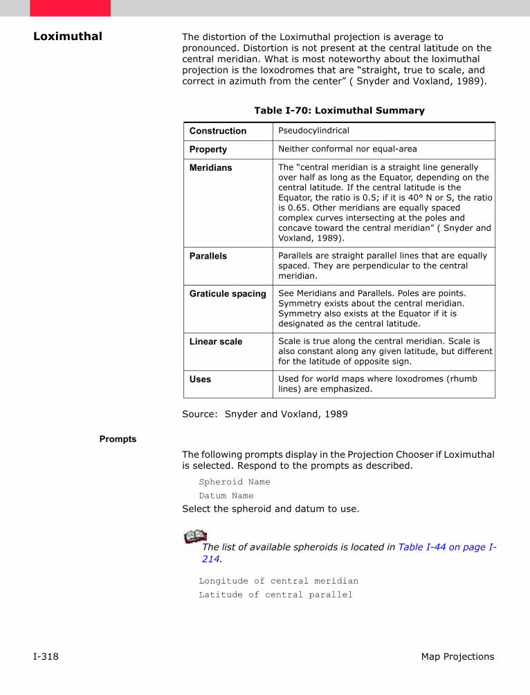
I-318 Map Projections

Loximuthal The distortion of the Loximuthal projection is average to pronounced. Distortion is not present at the central latitude on the central meridian. What is most noteworthy about the loximuthal projection is the loxodromes that are “straight, true to scale, and correct in azimuth from the center” ( Snyder and Voxland, 1989).

Source: Snyder and Voxland, 1989

PromptsThe following prompts display in the Projection Chooser if Loximuthal is selected. Respond to the prompts as described.

Spheroid Name

Datum Name

Select the spheroid and datum to use.

The list of available spheroids is located in Table I-44 on page I-214.

Longitude of central meridian

Latitude of central parallel

Table I-70: Loximuthal Summary

Construction Pseudocylindrical

Property Neither conformal nor equal-area

Meridians The “central meridian is a straight line generally over half as long as the Equator, depending on the central latitude. If the central latitude is the Equator, the ratio is 0.5; if it is 40° N or S, the ratio is 0.65. Other meridians are equally spaced complex curves intersecting at the poles and concave toward the central meridian” ( Snyder and Voxland, 1989).

Parallels Parallels are straight parallel lines that are equally spaced. They are perpendicular to the central meridian.

Graticule spacing See Meridians and Parallels. Poles are points. Symmetry exists about the central meridian. Symmetry also exists at the Equator if it is designated as the central latitude.

Linear scale Scale is true along the central meridian. Scale is also constant along any given latitude, but different for the latitude of opposite sign.

Uses Used for world maps where loxodromes (rhumb lines) are emphasized.

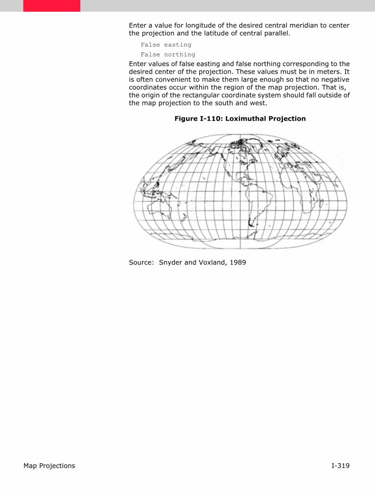
I-319Map Projections

Enter a value for longitude of the desired central meridian to center the projection and the latitude of central parallel.

False easting

False northing

Enter values of false easting and false northing corresponding to the desired center of the projection. These values must be in meters. It is often convenient to make them large enough so that no negative coordinates occur within the region of the map projection. That is, the origin of the rectangular coordinate system should fall outside of the map projection to the south and west.

Figure I-110: Loximuthal Projection

Source: Snyder and Voxland, 1989

I-320 Map Projections

Mercator This famous cylindrical projection was originally designed by Flemish map maker Gerhardus Mercator in 1569 to aid navigation (Figure I-111 on page I-322). Meridians and parallels are straight lines and cross at 90° angles. Angular relationships are preserved. However, to preserve conformality, parallels are placed increasingly farther apart with increasing distance from the Equator. Due to extreme scale distortion in high latitudes, the projection is rarely extended beyond 80°N or S unless the latitude of true scale is other than the Equator. Distance scales are usually furnished for several latitudes.

This projection can be thought of as being mathematically based on a cylinder tangent at the Equator. Any straight line is a constant-azimuth (rhumb) line. Areal enlargement is extreme away from the Equator; poles cannot be represented. Shape is true only within any small area. It is a reasonably accurate projection within a 15° band along the line of tangency.

Rhumb lines, which show constant direction, are straight. For this reason, a Mercator map was very valuable to sea navigators. However, rhumb lines are not the shortest path—great circles are the shortest path. Most great circles appear as long arcs when drawn on a Mercator map.

Table I-71: Mercator Summary

Construction Cylinder

Property Conformal

Meridians Meridians are straight and parallel.

Parallels Parallels are straight and parallel.

Graticule spacing

Meridian spacing is equal and the parallel spacing increases away from the Equator. The graticule spacing retains the property of conformality. The graticule is symmetrical. Meridians intersect parallels at right angles.

Linear scale

Linear scale is true along the Equator only (line of tangency), or along two parallels equidistant from the Equator (the secant form). Scale can be determined by measuring one degree of latitude, which equals 60 nautical miles, 69 statute miles, or 111 kilometers.

Uses

An excellent projection for equatorial regions. Otherwise, the Mercator is a special-purpose map projection best suited for navigation. Secant constructions are used for large-scale coastal charts. The use of the Mercator map projection as the base for nautical charts is universal. Examples are the charts published by the National Ocean Survey, US Dept. of Commerce.

I-321Map Projections

PromptsThe following prompts display in the Projection Chooser if Mercator is selected. Respond to the prompts as described.

Spheroid Name

Datum Name

Select the spheroid and datum to use.

The list of available spheroids is located in Table I-44 on page I-214.

Define the origin of the map projection in both spherical and rectangular coordinates.

Longitude of central meridian

Latitude of true scale

Enter values for longitude of the desired central meridian and latitude at which true scale is desired. Selection of a parameter other than the Equator can be useful for making maps in extreme north or south latitudes.

False easting at central meridian

False northing at origin

Enter values of false easting and false northing corresponding to the intersection of the central meridian and the latitude of true scale. These values must be in meters. It is often convenient to make them large enough so that no negative coordinates occur within the region of the map projection. That is, the origin of the rectangular coordinate system should fall outside of the map projection to the south and west.

I-322 Map Projections

Figure I-111: Mercator Projection

In Figure I-111 on page I-322, all angles are shown correctly, therefore small shapes are true (i.e., the map is conformal). Rhumb lines are straight, which makes it useful for navigation.

I-323Map Projections

Miller Cylindrical Miller Cylindrical is a modification of the Mercator projection (Figure I-112 on page I-324). It is similar to the Mercator from the Equator to 45°, but latitude line intervals are modified so that the distance between them increases less rapidly. Thus, beyond 45°, Miller Cylindrical lessens the extreme exaggeration of the Mercator. Miller Cylindrical also includes the poles as straight lines whereas the Mercator does not.

Meridians and parallels are straight lines intersecting at right angles. Meridians are equidistant, while parallels are spaced farther apart the farther they are from the Equator. Miller Cylindrical is not equal-area, equidistant, or conformal. Miller Cylindrical is used for world maps and in several atlases.

PromptsThe following prompts display in the Projection Chooser if Miller Cylindrical is selected. Respond to the prompts as described.

Spheroid Name

Datum Name

Select the spheroid and datum to use.

The list of available spheroids is located in Table I-44 on page I-214.

Longitude of central meridian

Table I-72: Miller Cylindrical Summary

Construction Cylinder

Property Compromise

Meridians All meridians are straight lines.

Parallels All parallels are straight lines.

Graticule spacing

Meridians are parallel and equally spaced, the lines of latitude are parallel, and the distance between them increases toward the poles. Both poles are represented as straight lines. Meridians and parallels intersect at right angles ( Environmental Systems Research Institute, 1992).

Linear scaleWhile the standard parallels, or lines, that are true to scale and free of distortion, are at latitudes 45°N and S, only the Equator is standard.

Uses Useful for world maps.

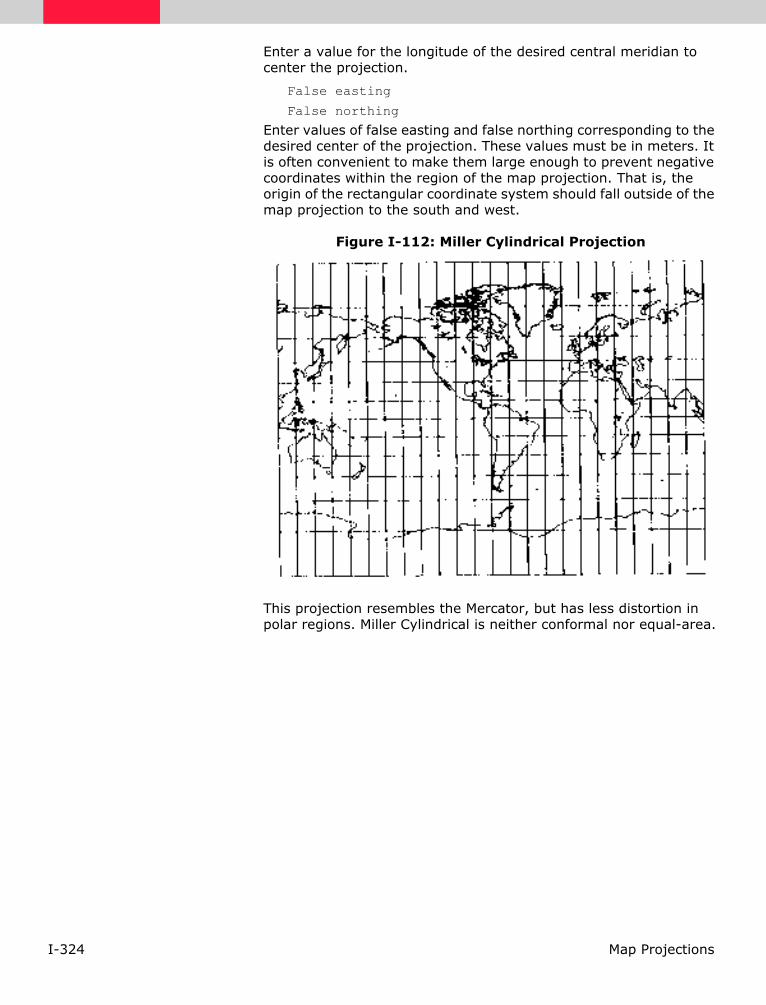
I-324 Map Projections

Enter a value for the longitude of the desired central meridian to center the projection.

False easting

False northing

Enter values of false easting and false northing corresponding to the desired center of the projection. These values must be in meters. It is often convenient to make them large enough to prevent negative coordinates within the region of the map projection. That is, the origin of the rectangular coordinate system should fall outside of the map projection to the south and west.

Figure I-112: Miller Cylindrical Projection

This projection resembles the Mercator, but has less distortion in polar regions. Miller Cylindrical is neither conformal nor equal-area.

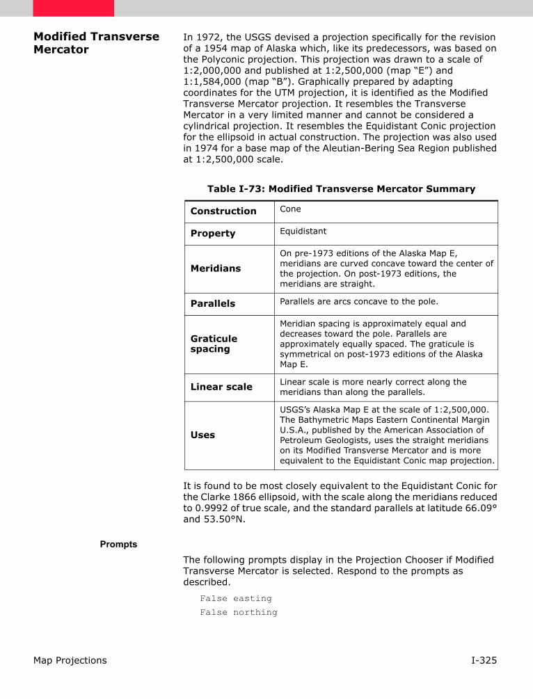
I-325Map Projections

Modified Transverse Mercator

In 1972, the USGS devised a projection specifically for the revision of a 1954 map of Alaska which, like its predecessors, was based on the Polyconic projection. This projection was drawn to a scale of 1:2,000,000 and published at 1:2,500,000 (map “E”) and 1:1,584,000 (map “B”). Graphically prepared by adapting coordinates for the UTM projection, it is identified as the Modified Transverse Mercator projection. It resembles the Transverse Mercator in a very limited manner and cannot be considered a cylindrical projection. It resembles the Equidistant Conic projection for the ellipsoid in actual construction. The projection was also used in 1974 for a base map of the Aleutian-Bering Sea Region published at 1:2,500,000 scale.

It is found to be most closely equivalent to the Equidistant Conic for the Clarke 1866 ellipsoid, with the scale along the meridians reduced to 0.9992 of true scale, and the standard parallels at latitude 66.09° and 53.50°N.

PromptsThe following prompts display in the Projection Chooser if Modified Transverse Mercator is selected. Respond to the prompts as described.

False easting

False northing

Table I-73: Modified Transverse Mercator Summary

Construction Cone

Property Equidistant

Meridians

On pre-1973 editions of the Alaska Map E, meridians are curved concave toward the center of the projection. On post-1973 editions, the meridians are straight.

Parallels Parallels are arcs concave to the pole.

Graticule spacing

Meridian spacing is approximately equal and decreases toward the pole. Parallels are approximately equally spaced. The graticule is symmetrical on post-1973 editions of the Alaska Map E.

Linear scale Linear scale is more nearly correct along the meridians than along the parallels.

Uses

USGS’s Alaska Map E at the scale of 1:2,500,000. The Bathymetric Maps Eastern Continental Margin U.S.A., published by the American Association of Petroleum Geologists, uses the straight meridians on its Modified Transverse Mercator and is more equivalent to the Equidistant Conic map projection.

I-326 Map Projections

Enter values of false easting and false northing corresponding to the desired center of the projection. These values must be in meters. It is often convenient to make them large enough to prevent negative coordinates within the region of the map projection. That is, the origin of the rectangular coordinate system should fall outside of the map projection to the south and west.

I-327Map Projections

Mollweide Carl B. Mollweide designed the projection in 1805. It is an equal-area pseudocylindrical projection. The Mollweide projection is used primarily for thematic maps of the world.

Source: Environmental Systems Research Institute, 1997

PromptsThe following prompts display in the Projection Chooser once Mollweide is selected. Respond to the prompts as described.

Spheroid Name

Datum Name

Select the spheroid and datum to use.

The list of available spheroids is located in Table I-44 on page I-214.

Longitude of central meridian

Enter a value for longitude of the desired central meridian.

False easting

False northing

Enter values of false easting and false northing corresponding to the desired center of the projection. These values must be in meters. It is often convenient to make them large enough so that no negative coordinates occur within the region of the map projection. That is, the origin of the rectangular coordinate system should fall outside of the map projection to the south and west.

Table I-74: Mollweide Summary

Construction Pseudocylinder

Property Equal-area

MeridiansMeridians are elliptical arcs that are equally spaced. The exception is the central meridian, which is a straight line.

Parallels All parallels are straight lines.

Graticule spacing

The Equator and the central meridian are linear graticules.

Linear scale

Scale is accurate along latitudes 40° 44’ N and S at the central meridian. Distortion becomes more pronounced farther from the lines, and is severe at the extremes of the projection.

Uses Use for world maps only.

I-328 Map Projections

Figure I-113: Mollweide Projection

Source: Snyder and Voxland, 1989

I-329Map Projections

New Zealand Map Grid

This projection is used only for mapping New Zealand.

Source: Environmental Systems Research Institute, 1997

PromptsThe following prompts display in the Projection Chooser once New Zealand Map Grid is selected. Respond to the prompts as described.

Spheroid Name

Datum Name

The Spheroid Name defaults to International 1909. The Datum Name defaults to Geodetic Datum 1949. These fields are not editable.

Easting Shift

Northing Shift

The Easting and Northing shifts are reported in meters.

Table I-75: New Zealand Map Grid Summary

Construction Modified cylindrical

Property Conformal

Meridians N/A

Parallels N/A

Graticule spacing None

Linear scale Scale is within 0.02 percent of actual scale for the country of New Zealand.

Uses This projection is useful only for maps of New Zealand.

I-330 Map Projections

Oblated Equal Area

PromptsThe following prompts display in the Projection Chooser once Oblated Equal Area is selected. Respond to the prompts as described.

Spheroid Name

Datum Name

Select the spheroid and datum to use.

Parameter M

Parameter N

Enter the oblated equal area oval shape of parameters M and N.

Longitude of center of projection

Latitude of center of projection

Enter the longitude of the center of the projection and the latitude of the center of the projection.

Rotation angle

Enter the oblated equal area oval rotation angle.

False easting

False northing

Enter values of false easting and false northing corresponding to the desired center of the projection. These values must be in meters. It is often convenient to make them large enough so that no negative coordinates occur within the region of the map projection. That is, the origin of the rectangular coordinate system should fall outside of the map projection to the south and west.

I-331Map Projections

Oblique Mercator (Hotine)

Oblique Mercator is a cylindrical, conformal projection that intersects the global surface along a great circle. It is equivalent to a Mercator projection that has been altered by rotating the cylinder so that the central line of the projection is a great circle path instead of the Equator. Shape is true only within any small area. Areal enlargement increases away from the line of tangency. Projection is reasonably accurate within a 15° band along the line of tangency.

The USGS uses the Hotine version of Oblique Mercator. The Hotine version is based on a study of conformal projections published by British geodesist Martin Hotine in 1946-47. Prior to the implementation of the Space Oblique Mercator, the Hotine version was used for mapping Landsat satellite imagery.

PromptsThe following prompts display in the Projection Chooser if Oblique Mercator (Hotine) is selected. Respond to the prompts as described.

Spheroid Name

Datum Name

Select the spheroid and datum to use.

Table I-76: Oblique Mercator (Hotine) Summary

Construction Cylinder

Property Conformal

MeridiansMeridians are complex curves concave toward the line of tangency, except each 180th meridian is straight.

Parallels Parallels are complex curves concave toward the nearest pole.

Graticule spacing

Graticule spacing increases away from the line of tangency and retains the property of conformality.

Linear scaleLinear scale is true along the line of tangency, or along two lines of equidistance from and parallel to the line of tangency.

Uses

Useful for plotting linear configurations that are situated along a line oblique to the Earth’s Equator. Examples are: NASA Surveyor Satellite tracking charts, ERTS flight indexes, strip charts for navigation, and the National Geographic Society’s maps “West Indies,” “Countries of the Caribbean,” “Hawaii,” and “New Zealand.”

I-332 Map Projections

The list of available spheroids is located in Table I-44 on page I-214.

Scale factor at center

Designate the desired scale factor along the central line of the projection. This parameter may be used to modify scale distortion away from this central line. A value of 1.0 indicates true scale only along the central line. A value of less than, but close to one is often used to lessen scale distortion away from the central line.

Latitude of point of origin

False easting

False northing

The center of the projection is defined by rectangular coordinates of false easting and false northing. The origin of rectangular coordinates on this projection occurs at the nearest intersection of the central line with the Earth’s Equator. To shift the origin to the intersection of the latitude of the origin entered above and the central line of the projection, compute coordinates of the latter point with zero false eastings and northings, reverse the signs of the coordinates obtained, and use these for false eastings and northings. These values must be in meters.

It is often convenient to add additional values so that no negative coordinates occur within the region of the map projection. That is, the origin of the rectangular coordinate system should fall outside of the map projection to the south and west.

Do you want to enter either:

A) Azimuth East of North for central line and the longitude of the point of origin

B) The latitude and longitude of the first and second points defining the central line

These formats differ slightly in definition of the central line of the projection.

Format A For format A, the additional prompts are:

Azimuth east of north for central line

Longitude of point of origin

Format A defines the central line of the projection by the angle east of north to the desired great circle path and by the latitude and longitude of the point along the great circle path from which the angle is measured. Appropriate values should be entered.

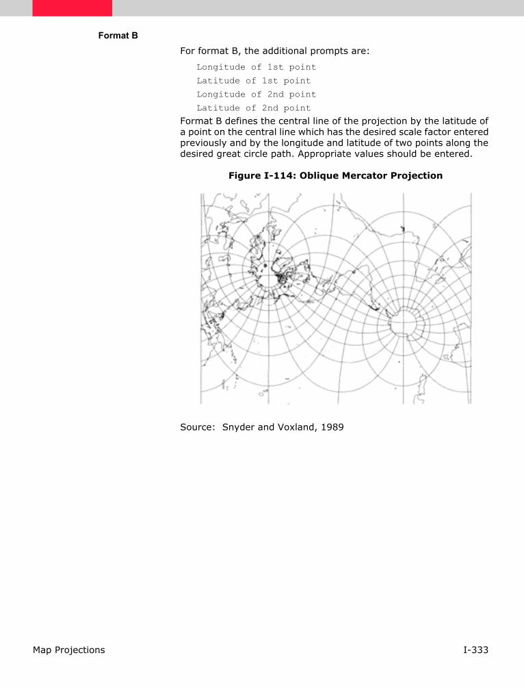
I-333Map Projections

Format B For format B, the additional prompts are:

Longitude of 1st point

Latitude of 1st point

Longitude of 2nd point

Latitude of 2nd point

Format B defines the central line of the projection by the latitude of a point on the central line which has the desired scale factor entered previously and by the longitude and latitude of two points along the desired great circle path. Appropriate values should be entered.

Figure I-114: Oblique Mercator Projection

Source: Snyder and Voxland, 1989

I-334 Map Projections

Orthographic The Orthographic projection is geometrically based on a plane tangent to the Earth, and the point of projection is at infinity (Figure I-115 on page I-336). The Earth appears as it would from outer space. Light rays that cast the projection are parallel and intersect the tangent plane at right angles. This projection is a truly graphic representation of the Earth, and is a projection in which distortion becomes a visual aid. It is the most familiar of the azimuthal map projections. Directions from the center of the projection are true.

This projection is limited to one hemisphere and shrinks those areas toward the periphery. In the polar aspect, latitude ring intervals decrease from the center outwards at a much greater rate than with Lambert Azimuthal. In the equatorial aspect, the central meridian and parallels are straight, with spaces closing up toward the outer edge.

The Orthographic projection seldom appears in atlases. Its utility is more pictorial than technical. Orthographic has been used as a basis for maps by Rand McNally and the USGS.

Table I-77: Orthographic Summary

Construction Plane

Property Compromise

Meridians

Polar aspect: the meridians are straight lines radiating from the point of tangency.

Oblique aspect: the meridians are ellipses, concave toward the center of the projection.

Equatorial aspect: the meridians are ellipses concave toward the straight central meridian.

Parallels

Polar aspect: the parallels are concentric circles.

Oblique aspect: the parallels are ellipses concave toward the poles.

Equatorial aspect: the parallels are straight and parallel.

Graticule spacing

Polar aspect: meridian spacing is equal and increases, and the parallel decreases from the point of tangency.

Oblique and equatorial aspects: the graticule spacing decreases away from the center of the projection.

Linear scale

Scale is true on the parallels in the polar aspect and on all circles centered at the pole of the projection in all aspects. Scale decreases along lines radiating from the center of the projection.

Uses USGS uses the Orthographic map projection in the National Atlas.

I-335Map Projections

PromptsThe following prompts display in the Projection Chooser if Orthographic is selected. Respond to the prompts as described.

Spheroid Name

Datum Name

Select the spheroid and datum to use.

The list of available spheroids is located in Table I-44 on page I-214.

Define the center of the map projection in both spherical and rectangular coordinates.

Longitude of center of projection

Latitude of center of projection

Enter values for the longitude and latitude of the desired center of the projection.

False easting

False northing

Enter values of false easting and false northing corresponding to the center of the projection. These values must be in meters. It is often convenient to make them large enough so that no negative coordinates occur within the region of the map projection. That is, the origin of the rectangular coordinate system should fall outside of the map projection to the south and west.Three views of the Orthographic projection are shown in Figure I-115 on page I-336: A) Polar aspect; B) Equatorial aspect; C) Oblique aspect, centered at 40°N and showing the classic globe-like view.

I-336 Map Projections

Figure I-115: Orthographic Projection

A

C

B

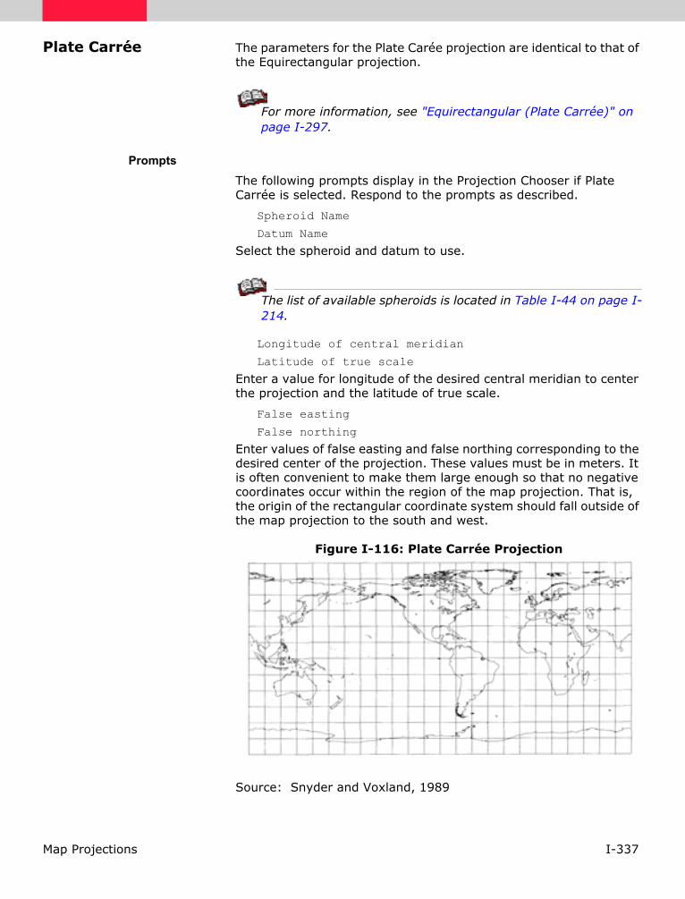
I-337Map Projections

Plate Carrée The parameters for the Plate Carée projection are identical to that of the Equirectangular projection.

For more information, see "Equirectangular (Plate Carrée)" on page I-297.

PromptsThe following prompts display in the Projection Chooser if Plate Carrée is selected. Respond to the prompts as described.

Spheroid Name

Datum Name

Select the spheroid and datum to use.

The list of available spheroids is located in Table I-44 on page I-214.

Longitude of central meridian

Latitude of true scale

Enter a value for longitude of the desired central meridian to center the projection and the latitude of true scale.

False easting

False northing

Enter values of false easting and false northing corresponding to the desired center of the projection. These values must be in meters. It is often convenient to make them large enough so that no negative coordinates occur within the region of the map projection. That is, the origin of the rectangular coordinate system should fall outside of the map projection to the south and west.

Figure I-116: Plate Carrée Projection

Source: Snyder and Voxland, 1989

I-338 Map Projections

Polar Stereographic The Polar Stereographic may be used to accommodate all regions not included in the UTM coordinate system, regions north of 84°N and 80°S. This form is called Universal Polar Stereographic (UPS). The projection is equivalent to the polar aspect of the Stereographic projection on a spheroid. The central point is either the North Pole or the South Pole. Of all the polar aspect planar projections, this is the only one that is conformal.

The point of tangency is a single point—either the North Pole or the South Pole. If the plane is secant instead of tangent, the point of global contact is a line of latitude ( Environmental Systems Research Institute, 1992).

Polar Stereographic is an azimuthal projection obtained by projecting from the opposite pole (Figure I-117 on page I-340). All of either the northern or southern hemispheres can be shown, but not both. This projection produces a circular map with one of the poles at the center.

Polar Stereographic stretches areas toward the periphery, and scale increases for areas farther from the central pole. Meridians are straight and radiating; parallels are concentric circles. Even though scale and area are not constant with Polar Stereographic, this projection, like all stereographic projections, possesses the property of conformality.

The Astrogeology Center of the Geological Survey at Flagstaff, Arizona, has been using the Polar Stereographic projection for the mapping of polar areas of every planet and satellite for which there is sufficient information.

Table I-78: Polar Stereographic Summary

Construction Plane

Property Conformal

Meridians Meridians are straight.

Parallels Parallels are concentric circles.

Graticule spacing

The distance between parallels increases with distance from the central pole.

Linear scale

The scale increases with distance from the center. If a standard parallel is chosen rather than one of the poles, this latitude represents the true scale, and the scale nearer the pole is reduced.

Uses

Polar regions (conformal). In the Universal Polar Stereographic (UPS) system, the scale factor at the pole is made 0.994, thus making the standard parallel (latitude of true scale) approximately 81°07’N or S.

I-339Map Projections

PromptsThe following prompts display in the Projection Chooser if Polar Stereographic is selected. Respond to the prompts as described.

Spheroid Name

Datum Name

Select the spheroid and datum to use.

The list of available spheroids is located in Table I-44 on page I-214.

Define the origin of the map projection in both spherical and rectangular coordinates. Ellipsoid projections of the polar regions normally use the International 1909 spheroid ( Environmental Systems Research Institute, 1992).

Longitude below pole of map

Enter a value for longitude directed straight down below the pole for a north polar aspect, or straight up from the pole for a south polar aspect. This is equivalent to centering the map with a desired meridian.

Latitude of true scale

Enter a value for latitude at which true scale is desired. For secant projections, specify the latitude of true scale as any line of latitude other than 90°N or S. For tangential projections, specify the latitude of true scale as the North Pole, 90 00 00, or the South Pole, -90 00 00 ( Environmental Systems Research Institute, 1992).

False easting

False northing

Enter values of false easting and false northing corresponding to the pole. These values must be in meters. It is often convenient to make them large enough to prevent negative coordinates within the region of the map projection. That is, the origin of the rectangular coordinate system should fall outside of the map projection to the south and west.This projection is conformal and is the most scientific projection for polar regions.

I-340 Map Projections

Figure I-117: Polar Stereographic Projection and its Geometric Construction

N. Pole

S. Pole

Plane of projection

Equator

I-341Map Projections

Polyconic Polyconic was developed in 1820 by Ferdinand Hassler specifically for mapping the eastern coast of the US (Figure I-118 on page I-342). Polyconic projections are made up of an infinite number of conic projections tangent to an infinite number of parallels. These conic projections are placed in relation to a central meridian. Polyconic projections compromise properties such as equal-area and conformality, although the central meridian is held true to scale.

This projection is used mostly for north-south oriented maps. Distortion increases greatly the farther east and west an area is from the central meridian.

PromptsThe following prompts display in the Projection Chooser if Polyconic is selected. Respond to the prompts as described.

Spheroid Name

Datum Name

Select the spheroid and datum to use.

The list of available spheroids is located in Table I-44 on page I-214.

Table I-79: Polyconic Summary

Construction Cone

Property Compromise

Meridians The central meridian is a straight line, but all other meridians are complex curves.

Parallels Parallels (except the Equator) are nonconcentric circular arcs. The Equator is a straight line.

Graticule spacing

All parallels are arcs of circles, but not concentric. All meridians, except the central meridian, are concave toward the central meridian. Parallels cross the central meridian at equal intervals but get farther apart at the east and west peripheries.

Linear scale

The scale along each parallel and along the central meridian of the projection is accurate. It increases along the meridians as the distance from the central meridian increases ( Environmental Systems Research Institute, 1992).

Uses

Used for 7.5-minute and 15-minute topographic USGS quad sheets, from 1886 to about 1957 ( Environmental Systems Research Institute, 1992). Used almost exclusively in slightly modified form for large-scale mapping in the United States until the 1950s.

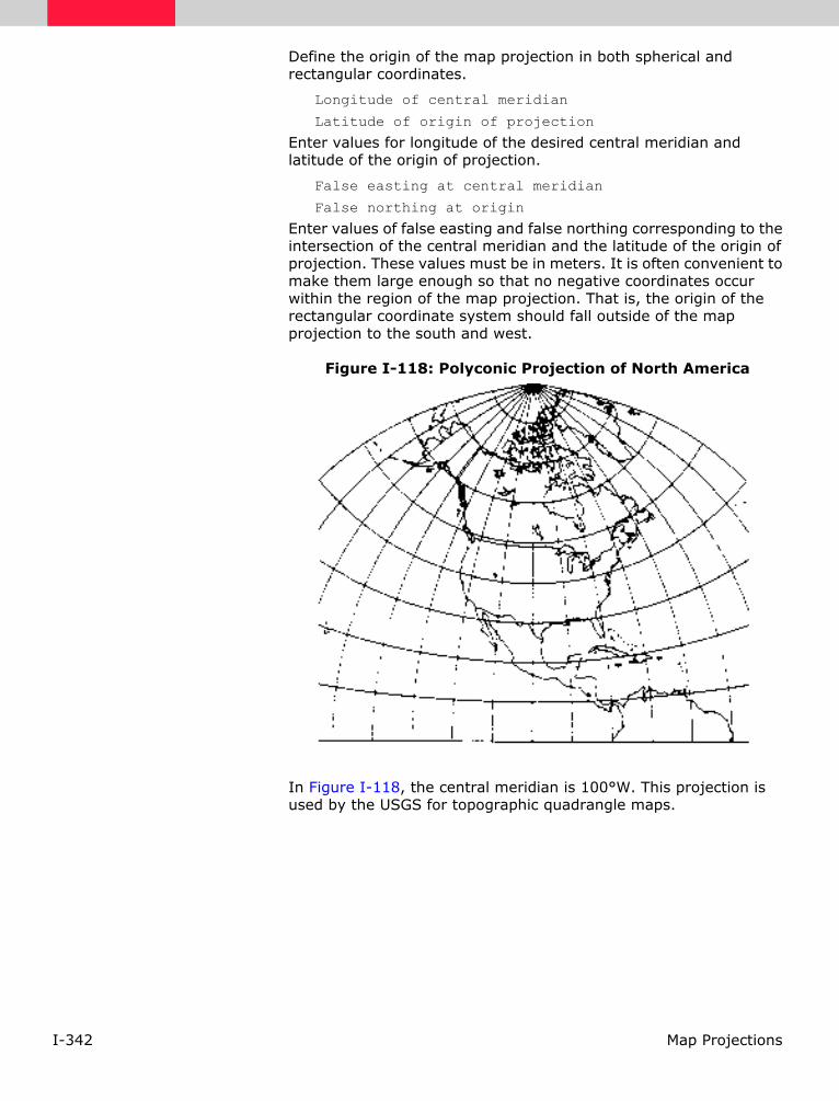
I-342 Map Projections

Define the origin of the map projection in both spherical and rectangular coordinates.

Longitude of central meridian

Latitude of origin of projection

Enter values for longitude of the desired central meridian and latitude of the origin of projection.

False easting at central meridian

False northing at origin

Enter values of false easting and false northing corresponding to the intersection of the central meridian and the latitude of the origin of projection. These values must be in meters. It is often convenient to make them large enough so that no negative coordinates occur within the region of the map projection. That is, the origin of the rectangular coordinate system should fall outside of the map projection to the south and west.

Figure I-118: Polyconic Projection of North America

In Figure I-118, the central meridian is 100°W. This projection is used by the USGS for topographic quadrangle maps.

I-343Map Projections

Quartic Authalic

Outer meridians at high latitudes have great distortion. If the Quartic Authalic projection is interrupted, distortion can be reduced.

Source: Snyder and Voxland, 1989

PromptsThe following prompts display in the Projection Chooser once Quartic Authalic is selected. Respond to the prompts as described.

Spheroid Name

Datum Name

Select the spheroid and datum to use.

The list of available spheroids is located in Table I-44 on page I-214.

Longitude of central meridian

Enter the value of the longitude of the central meridian.

False easting

False northing

Table I-80: Quartic Authalic

Construction Pseudocylindrical

Property Equal-area

Meridians The central meridian is a straight line, and is 0.45 as long as the Equator. The other meridians are curves that are equally spaced. They fit a “fourth-order (quartic) equation and concave toward the central meridian” ( Snyder and Voxland, 1989).

Parallels Parallels are straight parallel lines that are unequally spaced. The parallels have the greatest distance between in proximity to the Equator. Parallel spacing changes slowly, and parallels are perpendicular to the central meridian.

Graticule spacing See Meridians and Parallels. Poles are points. Symmetry exists about the central meridian or the Equator.

Linear scale Scale is accurate along the Equator. Scale is constant along each latitude, and is the same for the latitude of opposite sign.

Uses The McBryde-Thomas Flat-Polar Quartic projection uses Quartic Authalic as its base ( Snyder and Voxland, 1989). Used for world maps.

I-344 Map Projections

Enter values of false easting and false northing corresponding to the desired center of the projection. These values must be in meters. It is often convenient to make them large enough so that no negative coordinates occur within the region of the map projection. That is, the origin of the rectangular coordinate system should fall outside of the map projection to the south and west.

Figure I-119: Quartic Authalic Projection

Source: Snyder and Voxland, 1989

I-345Map Projections

Robinson According to ESRI, the Robinson “central meridian is a straight line 0.51 times the length of the Equator. Parallels are equally spaced straight lines between 38° N and S; spacing decreases beyond these limits. The poles are 0.53 times the length of the Equator. The projection is based upon tabular coordinates instead of mathematical formulas” ( Environmental Systems Research Institute, 1997).

This projection has been used both by Rand McNally and the National Geographic Society.

Source: Environmental Systems Research Institute, 1997

PromptsThe following prompts display in the Projection Chooser once Robinson is selected. Respond to the prompts as described.

Spheroid Name

Datum Name

Select the spheroid and datum to use.

The list of available spheroids is located in Table I-44 on page I-214.

Longitude of central meridian

Enter the value of the longitude of the central meridian.

False easting

False northing

Table I-81: Robinson Summary

Construction Pseudocylinder

Property Neither conformal nor equal-area

Meridians Meridians are equally spaced, and concave toward the central meridian, and look like elliptical arcs ( Environmental Systems Research Institute, 1997).

Parallels Parallels are equally spaced straight lines between 38° N and S.

Graticule spacing The central meridian and all parallels are linear.

Linear scale Scale is true along latitudes 38° N and S. Scale is constant along any specific latitude, and for the latitude of opposite sign.

Uses Useful for thematic and common world maps.

I-346 Map Projections

Enter values of false easting and false northing corresponding to the desired center of the projection. These values must be in meters. It is often convenient to make them large enough so that no negative coordinates occur within the region of the map projection. That is, the origin of the rectangular coordinate system should fall outside of the map projection to the south and west.

Figure I-120: Robinson Projection

Source: Snyder and Voxland, 1989

I-347Map Projections

RSO The acronym RSO stands for Rectified Skewed Orthomorphic. This projection is used to map areas of Brunei and Malaysia, and is each country’s national projection.

Source: Environmental Systems Research Institute, 1997

PromptsThe following prompts display in the Projection Chooser once RSO is selected. Respond to the prompts as described.

Spheroid Name

Datum Name

Select the spheroid and datum to use.

The list of available spheroids is located in Table I-44 on page I-214.

False easting

False northing

Enter values of false easting and false northing corresponding to the desired center of the projection. These values must be in meters. It is often convenient to make them large enough so that no negative coordinates occur within the region of the map projection. That is, the origin of the rectangular coordinate system should fall outside of the map projection to the south and west.

RSO Type

Select the RSO Type. You can choose from Borneo or Malaysia.

Table I-82: RSO Summary

Construction Cylinder

Property Conformal

Meridians Two meridians are 180 degrees apart.

Parallels N/A

Graticule spacing Graticules are two meridians 180 degrees apart.

Linear scale “A line of true scale is drawn at an angle to the central meridian” ( Environmental Systems Research Institute, 1997).

Uses This projection should be used to map areas of Brunei and Malaysia.

I-348 Map Projections

Sinusoidal Sometimes called the Sanson-Flamsteed, Sinusoidal is a projection with some characteristics of a cylindrical projection—often called a pseudocylindrical type. The central meridian is the only straight meridian—all others become sinusoidal curves. All parallels are straight and the correct length. Parallels are also the correct distance from the Equator, which, for a complete world map, is twice as long as the central meridian.

Sinusoidal maps achieve the property of equal-area but not conformality. The Equator and central meridian are distortion free, but distortion becomes pronounced near outer meridians, especially in polar regions.

Interrupting a Sinusoidal world or hemisphere map can lessen distortion. The interrupted Sinusoidal contains less distortion because each interrupted area can be constructed to contain a separate central meridian. Central meridians may be different for the northern and southern hemispheres and may be selected to minimize distortion of continents or oceans.

Sinusoidal is particularly suited for less than world areas, especially those bordering the Equator, such as South America or Africa. Sinusoidal is also used by the USGS as a base map for showing prospective hydrocarbon provinces and sedimentary basins of the world.

Table I-83: Sinusoidal Summary

Construction Pseudocylinder

Property Equal-area

Meridians Meridians are sinusoidal curves, curved toward a straight central meridian.

Parallels All parallels are straight, parallel lines.

Graticule spacing

Meridian spacing is equal and decreases toward the poles. Parallel spacing is equal. The graticule spacing retains the property of equivalence of area.

Linear scale Linear scale is true on the parallels and the central meridian.

Uses

Used as an equal-area projection to portray areas that have a maximum extent in a north-south direction. Used as a world equal-area projection in atlases to show distribution patterns. Used by the USGS as the base for maps showing prospective hydrocarbon provinces of the world, and sedimentary basins of the world.

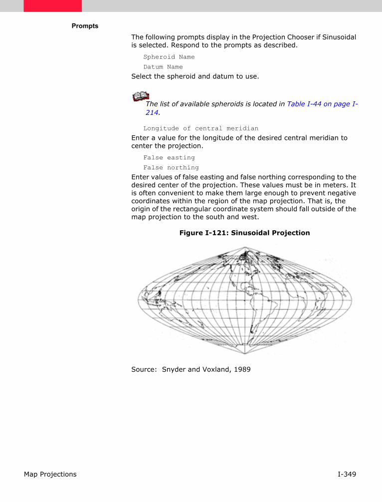
I-349Map Projections

PromptsThe following prompts display in the Projection Chooser if Sinusoidal is selected. Respond to the prompts as described.

Spheroid Name

Datum Name

Select the spheroid and datum to use.

The list of available spheroids is located in Table I-44 on page I-214.

Longitude of central meridian

Enter a value for the longitude of the desired central meridian to center the projection.

False easting

False northing

Enter values of false easting and false northing corresponding to the desired center of the projection. These values must be in meters. It is often convenient to make them large enough to prevent negative coordinates within the region of the map projection. That is, the origin of the rectangular coordinate system should fall outside of the map projection to the south and west.

Figure I-121: Sinusoidal Projection

Source: Snyder and Voxland, 1989

I-350 Map Projections

Space Oblique Mercator

The Space Oblique Mercator (SOM) projection is nearly conformal and has little scale distortion within the sensing range of an orbiting mapping satellite such as Landsat. It is the first projection to incorporate the Earth’s rotation with respect to the orbiting satellite.

The method of projection used is the modified cylindrical, for which the central line is curved and defined by the groundtrack of the orbit of the satellite.The line of tangency is conceptual and there are no graticules.

The SOM projection is defined by USGS. According to USGS, the X axis passes through the descending node for each daytime scene. The Y axis is perpendicular to the X axis, to form a Cartesian coordinate system. The direction of the X axis in a daytime Landsat scene is in the direction of the satellite motion—south. The Y axis is directed east. For SOM projections used by EOSAT, the axes are switched; the X axis is directed east and the Y axis is directed south.

The SOM projection is specifically designed to minimize distortion within sensing range of a mapping satellite as it orbits the Earth. It can be used for the rectification of, and continuous mapping from, satellite imagery. It is the standard format for data from Landsats 4 and 5. Plots for adjacent paths do not match without transformation (Environmental Systems Research Institute, 1991).

Table I-84: Space Oblique Mercator Summary

Construction Cylinder

Property Conformal

MeridiansAll meridians are curved lines except for the meridian crossed by the groundtrack at each polar approach.

Parallels All parallels are curved lines.

Graticule spacing

There are no graticules.

Linear scaleScale is true along the groundtrack, and varies approximately 0.01% within sensing range ( Environmental Systems Research Institute, 1992).

Uses

Used for georectification of, and continuous mapping from, satellite imagery. Standard format for data from Landsats 4 and 5 ( Environmental Systems Research Institute, 1992).

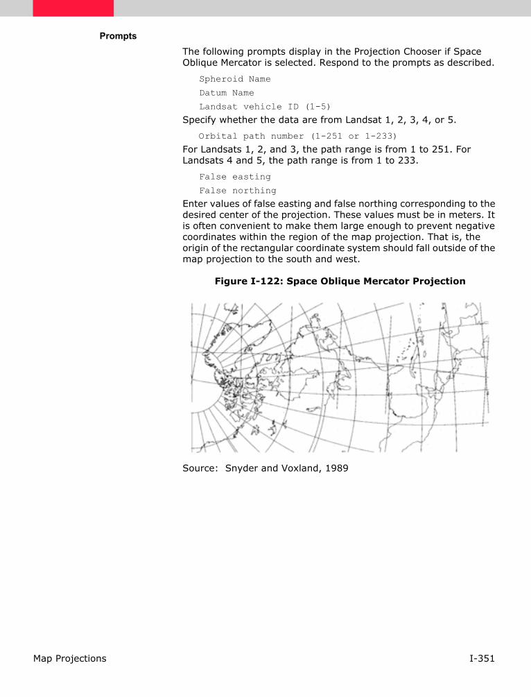
I-351Map Projections

PromptsThe following prompts display in the Projection Chooser if Space Oblique Mercator is selected. Respond to the prompts as described.

Spheroid Name

Datum Name

Landsat vehicle ID (1-5)

Specify whether the data are from Landsat 1, 2, 3, 4, or 5.

Orbital path number (1-251 or 1-233)

For Landsats 1, 2, and 3, the path range is from 1 to 251. For Landsats 4 and 5, the path range is from 1 to 233.

False easting

False northing

Enter values of false easting and false northing corresponding to the desired center of the projection. These values must be in meters. It is often convenient to make them large enough to prevent negative coordinates within the region of the map projection. That is, the origin of the rectangular coordinate system should fall outside of the map projection to the south and west.

Figure I-122: Space Oblique Mercator Projection

Source: Snyder and Voxland, 1989

I-352 Map Projections

Space Oblique Mercator (Formats A & B)

The Space Oblique Mercator (Formats A&B) projection is similar to the Space Oblique Mercator projection.

For more information, see "Space Oblique Mercator" on page I-350.

PromptsThe following prompts display in the Projection Chooser once Space Oblique Mercator (Formats A & B) is selected. Respond to the prompts as described.

Spheroid Name

Datum Name

Select the spheroid and datum to use.

False easting

False northing

Enter values of false easting and false northing corresponding to the desired center of the projection. These values must be in meters. It is often convenient to make them large enough so that no negative coordinates occur within the region of the map projection. That is, the origin of the rectangular coordinate system should fall outside of the map projection to the south and west.

Format A (Generic Satellite)

Inclination of orbit at ascending node

Period of satellite revolution in minutes

Longitude of ascending orbit at equator

Landsat path flag

If you select Format A of the Space Oblique Mercator projection, you need to supply the information listed above.

Format B (Landsat)

Landsat vehicle ID (1-5)

Specify whether the data are from Landsat 1, 2, 3, 4, or 5.

Path number (1-251 or 1-233)

For Landsats 1, 2, and 3, the path range is from 1 to 251. For Landsats 4 and 5, the path range is from 1 to 233.

I-353Map Projections

State Plane The State Plane is an X,Y coordinate system (not a map projection); its zones divide the US into over 130 sections, each with its own projection surface and grid network (Figure I-123 on page I-354). With the exception of very narrow states, such as Delaware, New Jersey, and New Hampshire, most states are divided into between two and ten zones. The Lambert Conformal projection is used for zones extending mostly in an east-west direction. The Transverse Mercator projection is used for zones extending mostly in a north-south direction. Alaska, Florida, and New York use either Transverse Mercator or Lambert Conformal for different areas. The Aleutian panhandle of Alaska is prepared on the Oblique Mercator projection.

Zone boundaries follow state and county lines, and, because each zone is small, distortion is less than one in 10,000. Each zone has a centrally located origin and a central meridian that passes through this origin. Two zone numbering systems are currently in use—the USGS code system and the National Ocean Service (NOS) code system (Table I-85, “NAD27 State Plane Coordinate System for the United States,” on page I-354 and Table I-86, “NAD83 State Plane Coordinate System for the United States,” on page I-358), but other numbering systems exist.

PromptsThe following prompts appear in the Projection Chooser if State Plane is selected. Respond to the prompts as described.

State Plane Zone

Enter either the USGS zone code number as a positive value, or the NOS zone code number as a negative value.

NAD27 or NAD83 or HARN

Either North America Datum 1927 (NAD27), North America Datum 1983 (NAD83), or High Accuracy Reference Network (HARN) may be used to perform the State Plane calculations.

• NAD27 is based on the Clarke 1866 spheroid.

• NAD83 and HARN are based on the GRS 1980 spheroid. Some zone numbers have been changed or deleted from NAD27.

Tables for both NAD27 and NAD83 zone numbers follow (Table I-85, “NAD27 State Plane Coordinate System for the United States,” on page I-354 and Table I-86, “NAD83 State Plane Coordinate System for the United States,” on page I-358). These tables include both USGS and NOS code systems.

I-354 Map Projections

Figure I-123: Zones of the State Plane Coordinate System

The following abbreviations are used in Table I-85, “NAD27 State Plane Coordinate System for the United States,” on page I-354 and Table I-86, “NAD83 State Plane Coordinate System for the United States,” on page I-358:

Tr Merc = Transverse Mercator

Lambert = Lambert Conformal Conic

Oblique = Oblique Mercator (Hotine)

Polycon = Polyconic

Table I-85: NAD27 State Plane Coordinate System for the United States

Code Number

State Zone Name Type USGS NOS

Alabama East Tr Merc 3101 -101

West Tr Merc 3126 -102

Alaska 1 Oblique 6101 -5001

2 Tr Merc 6126 -5002

3 Tr Merc 6151 -5003

4 Tr Merc 6176 -5004

5 Tr Merc 6201 -5005

6 Tr Merc 6226 -5006

7 Tr Merc 6251 -5007

8 Tr Merc 6276 -5008

9 Tr Merc 6301 -5009

10 Lambert 6326 -5010

American Samoa ------- Lambert ------ -5302

Arizona East Tr Merc 3151 -201

Central Tr Merc 3176 -202

West Tr Merc 3201 -203

I-355Map Projections

Arkansas North Lambert 3226 -301

South Lambert 3251 -302

California I Lambert 3276 -401

II Lambert 3301 -402

III Lambert 3326 -403

IV Lambert 3351 -404

V Lambert 3376 -405

VI Lambert 3401 -406

VII Lambert 3426 -407

Colorado North Lambert 3451 -501

Central Lambert 3476 -502

South Lambert 3501 -503

Connecticut -------- Lambert 3526 -600

Delaware -------- Tr Merc 3551 -700

District of Columbia Use Maryland or Virginia North

Florida East Tr Merc 3601 -901

West Tr Merc 3626 -902

North Lambert 3576 -903

Georgia East Tr Merc 3651 -1001

West Tr Merc 3676 -1002

Guam ------- Polycon ------- -5400

Hawaii 1 Tr Merc 5876 -5101

2 Tr Merc 5901 -5102

3 Tr Merc 5926 -5103

4 Tr Merc 5951 -5104

5 Tr Merc 5976 -5105

Idaho East Tr Merc 3701 -1101

Central Tr Merc 3726 -1102

West Tr Merc 3751 -1103

Illinois East Tr Merc 3776 -1201

West Tr Merc 3801 -1202

Indiana East Tr Merc 3826 -1301

West Tr Merc 3851 -1302

Table I-85: NAD27 State Plane Coordinate System for the United States (Continued)

Code Number

State Zone Name Type USGS NOS

I-356 Map Projections

Iowa North Lambert 3876 -1401

South Lambert 3901 -1402

Kansas North Lambert 3926 -1501

South Lambert 3951 -1502

Kentucky North Lambert 3976 -1601

South Lambert 4001 -1602

Louisiana North Lambert 4026 -1701

South Lambert 4051 -1702

Offshore Lambert 6426 -1703

Maine East Tr Merc 4076 -1801

West Tr Merc 4101 -1802

Maryland ------- Lambert 4126 -1900

Massachusetts Mainland Lambert 4151 -2001

Island Lambert 4176 -2002

Michigan (Tr Merc) East Tr Merc 4201 -2101

Central Tr Merc 4226 -2102

West Tr Merc 4251 -2103

Michigan (Lambert) North Lambert 6351 -2111

Central Lambert 6376 -2112

South Lambert 6401 -2113

Minnesota North Lambert 4276 -2201

Central Lambert 4301 -2202

South Lambert 4326 -2203

Mississippi East Tr Merc 4351 -2301

West Tr Merc 4376 -2302

Missouri East Tr Merc 4401 -2401

Central Tr Merc 4426 -2402

West Tr Merc 4451 -2403

Montana North Lambert 4476 -2501

Central Lambert 4501 -2502

South Lambert 4526 -2503

Nebraska North Lambert 4551 -2601

South Lambert 4576 -2602

Table I-85: NAD27 State Plane Coordinate System for the United States (Continued)

Code Number

State Zone Name Type USGS NOS

I-357Map Projections

Nevada East Tr Merc 4601 -2701

Central Tr Merc 4626 -2702

West Tr Merc 4651 -2703

New Hampshire --------- Tr Merc 4676 -2800

New Jersey --------- Tr Merc 4701 -2900

New Mexico East Tr Merc 4726 -3001

Central Tr Merc 4751 -3002

West Tr Merc 4776 -3003

New York East Tr Merc 4801 -3101

Central Tr Merc 4826 -3102

West Tr Merc 4851 -3103

Long Island Lambert 4876 -3104

North Carolina -------- Lambert 4901 -3200

North Dakota North Lambert 4926 -3301

South Lambert 4951 -3302

Ohio North Lambert 4976 -3401

South Lambert 5001 -3402

Oklahoma North Lambert 5026 -3501

South Lambert 5051 -3502

Oregon North Lambert 5076 -3601

South Lambert 5101 -3602

Pennsylvania North Lambert 5126 -3701

South Lambert 5151 -3702

Puerto Rico -------- Lambert 6001 -5201

Rhode Island -------- Tr Merc 5176 -3800

South Carolina North Lambert 5201 -3901

South Lambert 5226 -3902

South Dakota North Lambert 5251 -4001

South Lambert 5276 -4002

St. Croix --------- Lambert 6051 -5202

Tennessee --------- Lambert 5301 -4100

Table I-85: NAD27 State Plane Coordinate System for the United States (Continued)

Code Number

State Zone Name Type USGS NOS

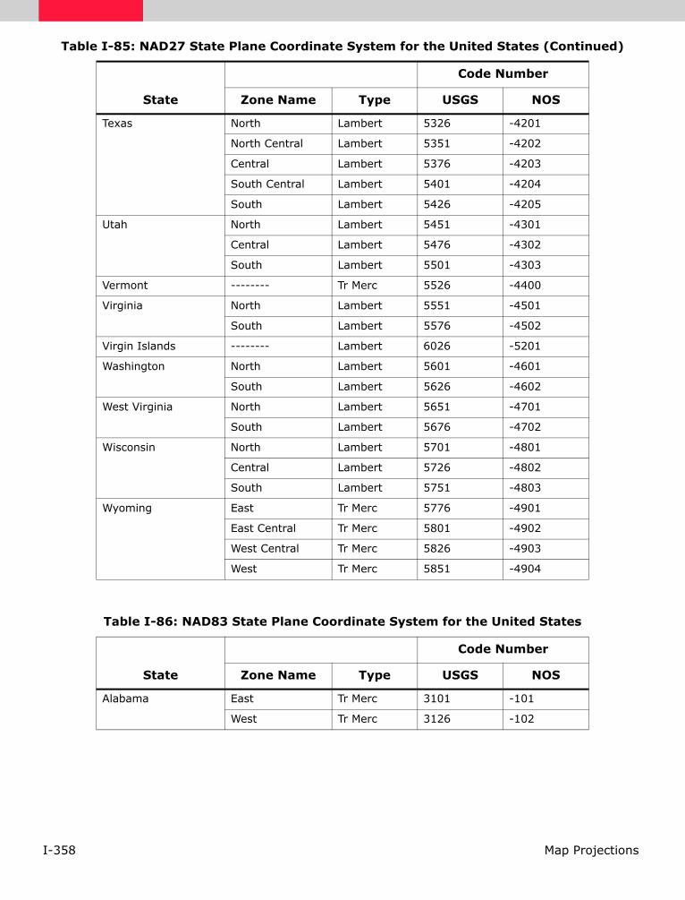
I-358 Map Projections

Texas North Lambert 5326 -4201

North Central Lambert 5351 -4202

Central Lambert 5376 -4203

South Central Lambert 5401 -4204

South Lambert 5426 -4205

Utah North Lambert 5451 -4301

Central Lambert 5476 -4302

South Lambert 5501 -4303

Vermont -------- Tr Merc 5526 -4400

Virginia North Lambert 5551 -4501

South Lambert 5576 -4502

Virgin Islands -------- Lambert 6026 -5201

Washington North Lambert 5601 -4601

South Lambert 5626 -4602

West Virginia North Lambert 5651 -4701

South Lambert 5676 -4702

Wisconsin North Lambert 5701 -4801

Central Lambert 5726 -4802

South Lambert 5751 -4803

Wyoming East Tr Merc 5776 -4901

East Central Tr Merc 5801 -4902

West Central Tr Merc 5826 -4903

West Tr Merc 5851 -4904

Table I-85: NAD27 State Plane Coordinate System for the United States (Continued)

Code Number

State Zone Name Type USGS NOS

Table I-86: NAD83 State Plane Coordinate System for the United States

Code Number

State Zone Name Type USGS NOS

Alabama East Tr Merc 3101 -101

West Tr Merc 3126 -102

I-359Map Projections

Alaska 1 Oblique 6101 -5001

2 Tr Merc 6126 -5002

3 Tr Merc 6151 -5003

4 Tr Merc 6176 -5004

5 Tr Merc 6201 -5005

6 Tr Merc 6226 -5006

7 Tr Merc 6251 -5007

8 Tr Merc 6276 -5008

9 Tr Merc 6301 -5009

10 Lambert 6326 -5010

Arizona East Tr Merc 3151 -201

Central Tr Merc 3176 -202

West Tr Merc 3201 -203

Arkansas North Lambert 3226 -301

South Lambert 3251 -302

California I Lambert 3276 -401

II Lambert 3301 -402

III Lambert 3326 -403

IV Lambert 3351 -404

V Lambert 3376 -405

VI Lambert 3401 -406

Colorado North Lambert 3451 -501

Central Lambert 3476 -502

South Lambert 3501 -503

Connecticut -------- Lambert 3526 -600

Delaware -------- Tr Merc 3551 -700

District of Columbia Use Maryland or Virginia North

Florida East Tr Merc 3601 -901

West Tr Merc 3626 -902

North Lambert 3576 -903

Georgia East Tr Merc 3651 -1001

West Tr Merc 3676 -1002

Table I-86: NAD83 State Plane Coordinate System for the United States (Continued)

Code Number

State Zone Name Type USGS NOS

I-360 Map Projections

Hawaii 1 Tr Merc 5876 -5101

2 Tr Merc 5901 -5102

3 Tr Merc 5926 -5103

4 Tr Merc 5951 -5104

5 Tr Merc 5976 -5105

Idaho East Tr Merc 3701 -1101

Central Tr Merc 3726 -1102

West Tr Merc 3751 -1103

Illinois East Tr Merc 3776 -1201

West Tr Merc 3801 -1202

Indiana East Tr Merc 3826 -1301

West Tr Merc 3851 -1302

Iowa North Lambert 3876 -1401

South Lambert 3901 -1402

Kansas North Lambert 3926 -1501

South Lambert 3951 -1502

Kentucky North Lambert 3976 -1601

South Lambert 4001 -1602

Louisiana North Lambert 4026 -1701

South Lambert 4051 -1702

Offshore Lambert 6426 -1703

Maine East Tr Merc 4076 -1801

West Tr Merc 4101 -1802

Maryland ------- Lambert 4126 -1900

Massachusetts Mainland Lambert 4151 -2001

Island Lambert 4176 -2002

Michigan North Lambert 6351 -2111

Central Lambert 6376 -2112

South Lambert 6401 -2113

Minnesota North Lambert 4276 -2201

Central Lambert 4301 -2202

South Lambert 4326 -2203

Mississippi East Tr Merc 4351 -2301

West Tr Merc 4376 -2302

Table I-86: NAD83 State Plane Coordinate System for the United States (Continued)

Code Number

State Zone Name Type USGS NOS

I-361Map Projections

Missouri East Tr Merc 4401 -2401

Central Tr Merc 4426 -2402

West Tr Merc 4451 -2403

Montana --------- Lambert 4476 -2500

Nebraska --------- Lambert 4551 -2600

Nevada East Tr Merc 4601 -2701

Central Tr Merc 4626 -2702

West Tr Merc 4651 -2703

New Hampshire --------- Tr Merc 4676 -2800

New Jersey --------- Tr Merc 4701 -2900

New Mexico East Tr Merc 4726 -3001

Central Tr Merc 4751 -3002

West Tr Merc 4776 -3003

New York East Tr Merc 4801 -3101

Central Tr Merc 4826 -3102

West Tr Merc 4851 -3103

Long Island Lambert 4876 -3104

North Carolina --------- Lambert 4901 -3200

North Dakota North Lambert 4926 -3301

South Lambert 4951 -3302

Ohio North Lambert 4976 -3401

South Lambert 5001 -3402

Oklahoma North Lambert 5026 -3501

South Lambert 5051 -3502

Oregon North Lambert 5076 -3601

South Lambert 5101 -3602

Pennsylvania North Lambert 5126 -3701

South Lambert 5151 -3702

Puerto Rico --------- Lambert 6001 -5201

Rhode Island --------- Tr Merc 5176 -3800

South Carolina --------- Lambert 5201 -3900

South Dakota --------- Lambert 5251 -4001

South Lambert 5276 -4002

Tennessee --------- Lambert 5301 -4100

Table I-86: NAD83 State Plane Coordinate System for the United States (Continued)

Code Number

State Zone Name Type USGS NOS

I-362 Map Projections

Texas North Lambert 5326 -4201

North Central Lambert 5351 -4202

Central Lambert 5376 -4203

South Central Lambert 5401 -4204

South Lambert 5426 -4205

Utah North Lambert 5451 -4301

Central Lambert 5476 -4302

South Lambert 5501 -4303

Vermont --------- Tr Merc 5526 -4400

Virginia North Lambert 5551 -4501

South Lambert 5576 -4502

Virgin Islands --------- Lambert 6026 -5201

Washington North Lambert 5601 -4601

South Lambert 5626 -4602

West Virginia North Lambert 5651 -4701

South Lambert 5676 -4702

Wisconsin North Lambert 5701 -4801

Central Lambert 5726 -4802

South Lambert 5751 -4803

Wyoming East Tr Merc 5776 -4901

East Central Tr Merc 5801 -4902

West Central Tr Merc 5826 -4903

West Tr Merc 5851 -4904

Table I-86: NAD83 State Plane Coordinate System for the United States (Continued)

Code Number

State Zone Name Type USGS NOS

I-363Map Projections

Stereographic Stereographic is a perspective projection in which points are projected from a position on the opposite side of the globe onto a plane tangent to the Earth (Figure I-124 on page I-365). All of one hemisphere can easily be shown, but it is impossible to show both hemispheres in their entirety from one center. It is the only azimuthal projection that preserves truth of angles and local shape. Scale increases and parallels become more widely spaced farther from the center.

In the equatorial aspect, all parallels except the Equator are circular arcs. In the polar aspect, latitude rings are spaced farther apart, with increasing distance from the pole.

Table I-87: Stereographic Summary

Construction Plane

Property Conformal

Meridians

Polar aspect: the meridians are straight lines radiating from the point of tangency.

Oblique and equatorial aspects: the meridians are arcs of circles concave toward a straight central meridian. In the equatorial aspect, the outer meridian of the hemisphere is a circle centered at the projection center.

Parallels

Polar aspect: the parallels are concentric circles.

Oblique aspect: the parallels are nonconcentric arcs of circles concave toward one of the poles with one parallel being a straight line.

Equatorial aspect: parallels are nonconcentric arcs of circles concave toward the poles; the Equator is straight.

Graticule spacing

The graticule spacing increases away from the center of the projection in all aspects and it retains the property of conformality.

Linear scale Scale increases toward the periphery of the projection.

Uses

The Stereographic projection is the most widely used azimuthal projection, mainly used for portraying large, continent-sized areas of similar extent in all directions. It is used in geophysics for solving problems in spherical geometry. The polar aspect is used for topographic maps and navigational charts. The American Geographical Society uses this projection as the basis for its “Map of the Arctic.” The USGS uses it as the basis for maps of Antarctica.

I-364 Map Projections

PromptsThe following prompts display in the Projection Chooser if Stereographic is selected. Respond to the prompts as described.

Spheroid Name

Datum Name

Select the spheroid and datum to use.

The list of available spheroids is located in Table I-44 on page I-214.

Define the center of the map projection in both spherical and rectangular coordinates.

Longitude of center of projection

Latitude of center of projection

Enter values for the longitude and latitude of the desired center of the projection.

False easting

False northing

Enter values of false easting and false northing corresponding to the center of the projection. These values must be in meters. It is often convenient to make them large enough so that no negative coordinates occur within the region of the map projection. That is, the origin of the rectangular coordinate system should fall outside of the map projection to the south and west.

The Stereographic is the only azimuthal projection which is conformal. Figure I-124 on page I-365 shows two views: A) Equatorial aspect, often used in the 16th and 17th centuries for maps of hemispheres; and B) Oblique aspect, centered on 40°N.

I-365Map Projections

Figure I-124: Stereographic Projection

A

B

I-366 Map Projections

Stereographic (Extended)

The Stereographic (Extended) projection has the same attributes as the Stereographic projection, with the exception of the ability to define scale factors.

For details about the Stereographic projection, see "Stereographic" on page I-363.

PromptsThe following prompts display in the Projection Chooser once Stereographic (Extended) is selected. Respond to the prompts as described.

Spheroid Name

Datum Name

Select the spheroid and datum to use.

The list of available spheroids is located in Table I-44 on page I-214.

Scale factor

Designate the desired scale factor. This parameter is used to modify scale distortion. A value of one indicates true scale only along the central meridian. It may be desirable to have true scale along two lines equidistant from and parallel to the central meridian, or to lessen scale distortion away from the central meridian. A factor of less than, but close to one is often used.

Longitude of origin of projection

Latitude of origin of projection

Enter the values for longitude of origin of projection and latitude of origin of projection.

False easting

False northing

Enter values of false easting and false northing corresponding to the desired center of the projection. These values must be in meters. It is often convenient to make them large enough so that no negative coordinates occur within the region of the map projection. That is, the origin of the rectangular coordinate system should fall outside of the map projection to the south and west.

I-367Map Projections

Transverse Mercator Transverse Mercator is similar to the Mercator projection except that the axis of the projection cylinder is rotated 90° from the vertical (polar) axis. The contact line is then a chosen meridian instead of the Equator, and this central meridian runs from pole to pole. It loses the properties of straight meridians and straight parallels of the standard Mercator projection (except for the central meridian, the two meridians 90° away, and the Equator).

Transverse Mercator also loses the straight rhumb lines of the Mercator map, but it is a conformal projection. Scale is true along the central meridian or along two straight lines equidistant from, and parallel to, the central meridian. It cannot be edge-joined in an east-west direction if each sheet has its own central meridian.

In the United States, Transverse Mercator is the projection used in the State Plane coordinate system for states with predominant north-south extent. The entire Earth from 84°N to 80°S is mapped with a system of projections called the Universal Transverse Mercator.

PromptsThe following prompts display in the Projection Chooser if Transverse Mercator is selected. Respond to the prompts as described.

Spheroid Name

Datum Name

Select the spheroid and datum to use.

Table I-88: Transverse Mercator Summary

Construction Cylinder

Property Conformal

Meridians

Meridians are complex curves concave toward a straight central meridian that is tangent to the globe. The straight central meridian intersects the Equator and one meridian at a 90° angle.

Parallels Parallels are complex curves concave toward the nearest pole; the Equator is straight.

Graticule spacing

Parallels are spaced at their true distances on the straight central meridian. Graticule spacing increases away from the tangent meridian. The graticule retains the property of conformality.

Linear scaleLinear scale is true along the line of tangency, or along two lines equidistant from, and parallel to, the line of tangency.

Uses

Used where the north-south dimension is greater than the east west dimension. Used as the base for the USGS 1:250,000-scale series, and for some of the 7.5-minute and 15-minute quadrangles of the National Topographic Map Series.

I-368 Map Projections

The list of available spheroids is located in Table I-44 on page I-214.

Scale factor at central meridian

Designate the desired scale factor at the central meridian. This parameter is used to modify scale distortion. A value of one indicates true scale only along the central meridian. It may be desirable to have true scale along two lines equidistant from and parallel to the central meridian, or to lessen scale distortion away from the central meridian. A factor of less than, but close to one is often used.

Finally, define the origin of the map projection in both spherical and rectangular coordinates.

Longitude of central meridian

Latitude of origin of projection

Enter values for longitude of the desired central meridian and latitude of the origin of projection.

False easting

False northing

Enter values of false easting and false northing corresponding to the intersection of the central meridian and the latitude of the origin of projection. These values must be in meters. It is often convenient to make them large enough so that there are no negative coordinates within the region of the map projection. That is, origin of the rectangular coordinate system should fall outside of the map projection to the south and west.

I-369Map Projections

Two Point Equidistant

The Two Point Equidistant projection is used to show the distance from “either of two chosen points to any other point on a map” ( Environmental Systems Research Institute, 1997). Note that the first point has to be west of the second point. This projection has been used by the National Geographic Society to map areas of Asia.

Source: Environmental Systems Research Institute, 1997

PromptsThe following prompts display in the Projection Chooser once Two Point Equidistant is selected. Respond to the prompts as described.

Spheroid Name

Datum Name

Select the spheroid and datum to use.

The list of available spheroids is located in Table I-44 on page I-214.

False easting

False northing

Enter values of false easting and false northing corresponding to the desired center of the projection. These values must be in meters. It is often convenient to make them large enough so that no negative coordinates occur within the region of the map projection. That is, the origin of the rectangular coordinate system should fall outside of the map projection to the south and west.

Longitude of 1st point

Latitude of 1st point

Table I-89: Two Point Equidistant Summary

Construction Modified planar

Property Compromise

Meridians N/A

Parallels N/A

Graticule spacing

N/A

Linear scale N/A

Uses

The Two Point Equidistant projection “does not represent great circle paths” ( Environmental Systems Research Institute, 1997). There is little distortion if two chosen points are within 45 degrees of each other.

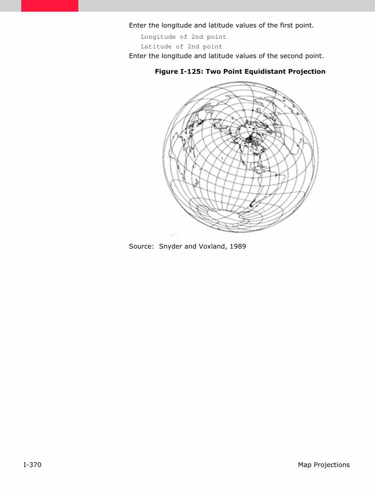
I-370 Map Projections

Enter the longitude and latitude values of the first point.

Longitude of 2nd point

Latitude of 2nd point

Enter the longitude and latitude values of the second point.

Figure I-125: Two Point Equidistant Projection

Source: Snyder and Voxland, 1989

I-371Map Projections

UTM UTM is an international plane (rectangular) coordinate system developed by the US Army that extends around the world from 84°N to 80°S. The world is divided into 60 zones each covering six degrees longitude. Each zone extends three degrees eastward and three degrees westward from its central meridian. Zones are numbered consecutively west to east from the 180° meridian (Figure I-126, Table I-90, “UTM Zones, Central Meridians, and Longitude Ranges,” on page I-372).

The Transverse Mercator projection is then applied to each UTM zone. Transverse Mercator is a transverse form of the Mercator cylindrical projection. The projection cylinder is rotated 90° from the vertical (polar) axis and can then be placed to intersect at a chosen central meridian. The UTM system specifies the central meridian of each zone. With a separate projection for each UTM zone, a high degree of accuracy is possible (one part in 1000 maximum distortion within each zone). If the map to be projected extends beyond the border of the UTM zone, the entire map may be projected for any UTM zone specified by you.

See "Transverse Mercator" on page I-367 for more information.

PromptsThe following prompts display in the Projection Chooser if UTM is chosen.

Spheroid Name

Datum Name

Select the spheroid and datum to use.

The list of available spheroids is located in Table I-44 on page I-214.

UTM Zone

North or South

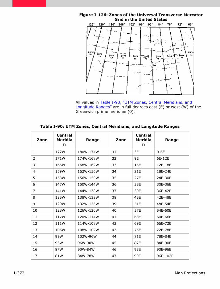
I-372 Map Projections

Figure I-126: Zones of the Universal Transverse Mercator Grid in the United States

All values in Table I-90, “UTM Zones, Central Meridians, and Longitude Ranges” are in full degrees east (E) or west (W) of the Greenwich prime meridian (0).

126° 120° 114° 108° 102° 96° 90° 84° 78° 72° 66°

Table I-90: UTM Zones, Central Meridians, and Longitude Ranges

ZoneCentral Meridia

nRange Zone

Central Meridia

nRange

1 177W 180W-174W 31 3E 0-6E

2 171W 174W-168W 32 9E 6E-12E

3 165W 168W-162W 33 15E 12E-18E

4 159W 162W-156W 34 21E 18E-24E

5 153W 156W-150W 35 27E 24E-30E

6 147W 150W-144W 36 33E 30E-36E

7 141W 144W-138W 37 39E 36E-42E

8 135W 138W-132W 38 45E 42E-48E

9 129W 132W-126W 39 51E 48E-54E

10 123W 126W-120W 40 57E 54E-60E

11 117W 120W-114W 41 63E 60E-66E

12 111W 114W-108W 42 69E 66E-72E

13 105W 108W-102W 43 75E 72E-78E

14 99W 102W-96W 44 81E 78E-84E

15 93W 96W-90W 45 87E 84E-90E

16 87W 90W-84W 46 93E 90E-96E

17 81W 84W-78W 47 99E 96E-102E

I-373Map Projections

18 75W 78W-72W 48 105E 102E-108E

19 69W 72W-66W 49 111E 108E-114E

20 63W 66W-60W 50 117E 114E-120E

21 57W 60W-54W 51 123E 120E-126E

22 51W 54W-48W 52 129E 126E-132E

23 45W 48W-42W 53 135E 132E-138E

24 39W 42W-36W 54 141E 138E-144E

25 33W 36W-30W 55 147E 144E-150E

26 27W 30W-24W 56 153E 150E-156E

27 21W 24W-18W 57 159E 156E-162E

28 15W 18W-12W 58 165E 162E-168E

29 9W 12W-6W 59 171E 168E-174E

30 3W 6W-0 60 177E 174E-180E

Table I-90: UTM Zones, Central Meridians, and Longitude Ranges (Continued)

ZoneCentral Meridia

nRange Zone

Central Meridia

nRange

I-374 Map Projections

Van der Grinten I The Van der Grinten I projection produces a map that is neither conformal nor equal-area (Figure I-127 on page I-375). It compromises all properties, and represents the Earth within a circle.

All lines are curved except the central meridian and the Equator. Parallels are spaced farther apart toward the poles. Meridian spacing is equal at the Equator. Scale is true along the Equator, but increases rapidly toward the poles, which are usually not represented.

Van der Grinten I avoids the excessive stretching of the Mercator and the shape distortion of many of the equal-area projections. It has been used to show distribution of mineral resources on the ocean floor.

PromptsThe following prompts display in the Projection Chooser if Van der Grinten I is selected. Respond to the prompts as described.

Spheroid Name

Datum Name

Select the spheroid and datum to use.

The list of available spheroids is located in Table I-44 on page I-214.

Longitude of central meridian

Table I-91: Van der Grinten I Summary

Construction Miscellaneous

Property Compromise

Meridians Meridians are circular arcs concave toward a straight central meridian.

Parallels Parallels are circular arcs concave toward the poles, except for a straight Equator.

Graticule spacing

Meridian spacing is equal at the Equator. The parallels are spaced farther apart toward the poles. The central meridian and Equator are straight lines. The poles are commonly not represented. The graticule spacing results in a compromise of all properties.

Linear scale Linear scale is true along the Equator. Scale increases rapidly toward the poles.

Uses

The Van der Grinten projection is used by the National Geographic Society for world maps. Used by the USGS to show distribution of mineral resources on the sea floor.

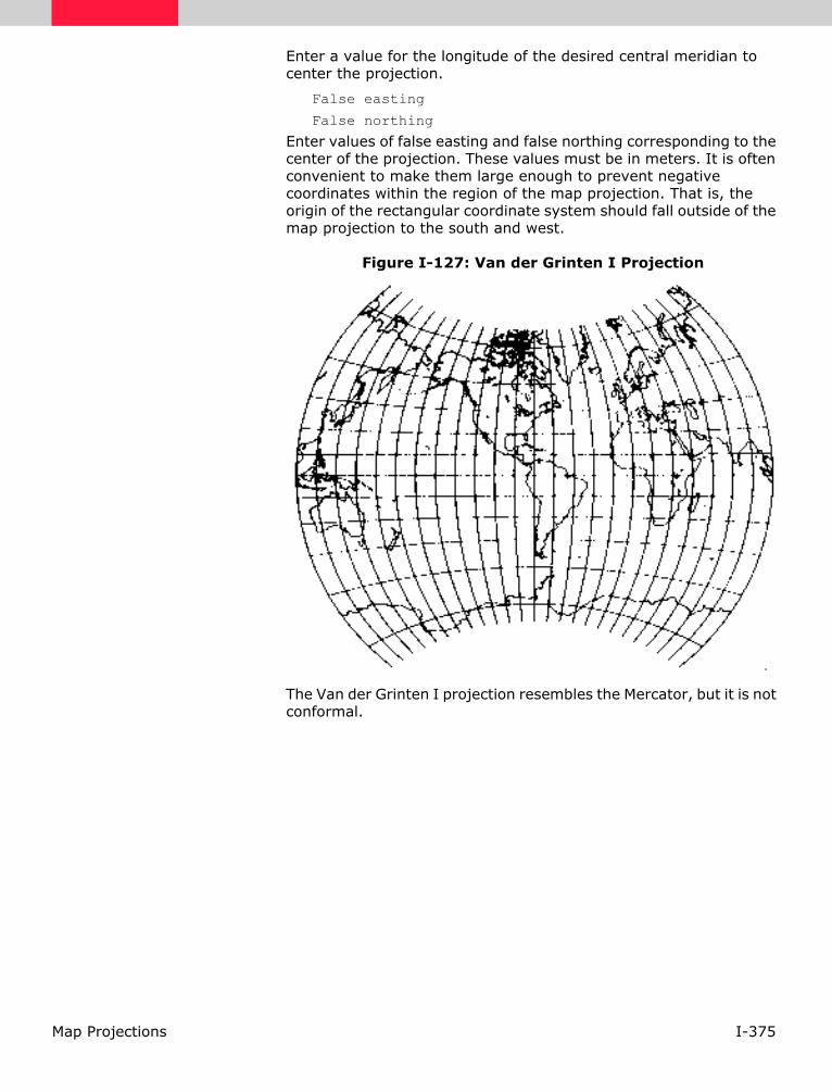
I-375Map Projections

Enter a value for the longitude of the desired central meridian to center the projection.

False easting

False northing

Enter values of false easting and false northing corresponding to the center of the projection. These values must be in meters. It is often convenient to make them large enough to prevent negative coordinates within the region of the map projection. That is, the origin of the rectangular coordinate system should fall outside of the map projection to the south and west.

Figure I-127: Van der Grinten I Projection

The Van der Grinten I projection resembles the Mercator, but it is not conformal.

I-376 Map Projections

Wagner IV

The Wagner IV Projection has distortion primarily in the polar regions.

Source: Snyder and Voxland, 1989

PromptsThe following prompts display in the Projection Chooser if Wagner IV is selected. Respond to the prompts as described.

Spheroid Name

Datum Name

Select the spheroid and datum to use.

The list of available spheroids is located in Table I-44 on page I-214.

Longitude of central meridian

Enter a value for the longitude of the desired central meridian to center the projection.

False easting

False northing

Table I-92: Wagner IV Summary

Construction Pseudocylinder

Property Equal-area

Meridians The central meridian is a straight line one half as long as the Equator. The other meridians are portions of ellipses that are equally spaced. They are concave towards the central meridian. The meridians at 103° 55’ E and W of the central meridian are circular arcs.

Parallels Parallels are unequally spaced. Parallels have the widest space between them at the Equator, and are perpendicular to the central meridian.

Graticule spacing See Meridians and Parallels. Poles are lines one half as long as the Equator. Symmetry exists around the central meridian or the Equator.

Linear scale Scale is accurate along latitudes 42° 59’ N and S. Scale is constant along any specific latitude as well as the latitude of opposite sign.

Uses Useful for world maps.

I-377Map Projections

Enter values of false easting and false northing corresponding to the center of the projection. These values must be in meters. It is often convenient to make them large enough to prevent negative coordinates within the region of the map projection. That is, the origin of the rectangular coordinate system should fall outside of the map projection to the south and west.

Figure I-128: Wagner IV Projection

Source: Snyder and Voxland, 1989

I-378 Map Projections

Wagner VII The Wagner VII projection is modified based on the Hammer projection. “The poles correspond to the 65th parallels on the Hammer [projection], and meridians are repositioned” ( Snyder and Voxland, 1989).

Distortion is prevalent in polar areas.

Source: Snyder and Voxland, 1989

PromptsThe following prompts display in the Projection Chooser if Wagner IV is selected. Respond to the prompts as described.

Spheroid Name

Datum Name

Select the spheroid and datum to use.

The list of available spheroids is located in Table I-44 on page I-214.

Longitude of central meridian

Enter a value for the longitude of the desired central meridian to center the projection.

False easting

False northing

Table I-93: Wagner VII

Construction Modified azimuthal

Property Equal-area

Meridians Central meridian is straight and half the Equator’s length. Other meridians are unequally spaced curves. They are concave toward the central meridian.

Parallels The Equator is straight; the other parallels are curved. Other parallels are unequally spaced curves, which are concave toward the closest pole.

Graticule spacing See Meridians and Parallels. Poles are curved lines. Symmetry exists about the central meridian or the Equator.

Linear scale Scale decreases along the central meridian and the Equator relative to distance from the center of the Wagner VII projection.

Uses Used for world maps.

I-379Map Projections

Enter values of false easting and false northing corresponding to the center of the projection. These values must be in meters. It is often convenient to make them large enough to prevent negative coordinates within the region of the map projection. That is, the origin of the rectangular coordinate system should fall outside of the map projection to the south and west.

Figure I-129: Wagner VII Projection

Source: Snyder and Voxland, 1989

I-380 Map Projections

Winkel I

The Winkel I projection is “not free of distortion at any point” ( Snyder and Voxland, 1989).

Source: Snyder and Voxland, 1989

PromptsThe following prompts display in the Projection Chooser once Winkel I is selected. Respond to the prompts as described.

Spheroid Name

Datum Name

Select the spheroid and datum to use.

The list of available spheroids is located in Table I-44 on page I-214.

Latitude of standard parallel

Longitude of central meridian

Enter values of the latitude of standard parallel and the longitude of central meridian.

False easting

False northing

Enter values of false easting and false northing corresponding to the desired center of the projection. These values must be in meters. It is often convenient to make them large enough so that no negative coordinates occur within the region of the map projection. That is, the origin of the rectangular coordinate system should fall outside of the map projection to the south and west.

Table I-94: Winkel I Summary

Construction Pseudocylinder

Property Neither conformal nor equal-area

Meridians Central meridian is a straight line 0.61 the length of the Equator. The other meridians are sinusoidal curves that are equally spaced and concave toward the central meridian.

Parallels Parallels are equally spaced.

Graticule spacing See Meridians and Parallels. Pole lines are 0.61 the length of the Equator. Symmetry exists about the central meridian or the Equator.

Linear scale Scale is true along latitudes 50° 28’ N and S. Scale is constant along any given latitude as well as the latitude of the opposite sign.

Uses Used for world maps.

I-381Map Projections

Figure I-130: Winkel I Projection

Source: Snyder and Voxland, 1989

I-382 Map Projections

External Projections The following external projections are supported in ERDAS IMAGINE and are described in this section. Some of these projections were discussed in the previous section. Those descriptions are not repeated here. Simply refer to the page number in parentheses for more information.

NOTE: ERDAS IMAGINE does not support datum shifts for these external projections.

• Albers Equal Area (see "Albers Conical Equal Area" on page I-269)

• Azimuthal Equidistant (see "Azimuthal Equidistant" on page I-272)

• Bipolar Oblique Conic Conformal

• Cassini-Soldner

• Conic Equidistant (see "Equidistant Conic" on page I-294)

• Laborde Oblique Mercator

• Lambert Azimuthal Equal Area (see "Lambert Azimuthal Equal Area" on page I-312)

• Lambert Conformal Conic (see "Lambert Conformal Conic" on page I-315)

• Mercator (see "Mercator" on page I-320)

• Minimum Error Conformal

• Modified Polyconic

• Modified Stereographic

• Mollweide Equal Area (see "Mollweide" on page I-327)

• Oblique Mercator (see "Oblique Mercator (Hotine)" on page I-331)

• Orthographic (see "Orthographic" on page I-334)

• Plate Carrée (see "Equirectangular (Plate Carrée)" on page I-297)

• Rectified Skew Orthomorphic (see "RSO" on page I-347)

• Regular Polyconic (see "Polyconic" on page I-341)

• Robinson Pseudocylindrical (see "Robinson" on page I-345)

• Sinusoidal (see "Sinusoidal" on page I-348)

I-383Map Projections

• Southern Orientated Gauss Conformal

• Stereographic (see "Stereographic" on page I-363)

• Swiss Cylindrical

• Stereographic (Oblique) (see "Stereographic" on page I-363)

• Transverse Mercator (see "Transverse Mercator" on page I-367)

• Universal Transverse Mercator (see "UTM" on page I-371)

• Van der Grinten (see "Van der Grinten I" on page I-374)

• Winkel’s Tripel

I-384 Map Projections

Bipolar Oblique Conic Conformal

The Bipolar Oblique Conic Conformal projection was developed by O.M. Miller and William A. Briesemeister in 1941 specifically for mapping North and South America, and maintains conformality for these regions. It is based upon the Lambert Conformal Conic, using two oblique conic projections side-by-side.

The two oblique conics are joined with the poles 104° apart. A great circle arc 104° long begins at 20°S and 110°W, cuts through Central America, and terminates at 45°N and approximately 19°59’36”W. The scale of the map is then increased by approximately 3.5%. The origin of the coordinates is made 17°15’N, 73°02’W.

Refer to "Lambert Conformal Conic" on page I-315 for more information.

PromptsThe following prompts display in the Projection Chooser if Bipolar Oblique Conic Conformal is selected.

Projection Name

Spheroid Type

Datum Name

Table I-95: Bipolar Oblique Conic Conformal Summary

Construction Cone

Property Conformal

Meridians Meridians are complex curves concave toward the center of the projection.

Parallels Parallels are complex curves concave toward the nearest pole.

Graticule spacing

Graticule spacing increases away from the lines of true scale and retains the property of conformality.

Linear scale

Linear scale is true along two lines that do not lie along any meridian or parallel. Scale is compressed between these lines and expanded beyond them. Linear scale is generally good, but there is as much as a 10% error at the edge of the projection as used.

Uses

Used to represent one or both of the American continents. Examples are the Basement map of North America and the Tectonic map of North America.

I-385Map Projections

Cassini-Soldner The Cassini projection was devised by C. F. Cassini de Thury in 1745 for the survey of France. Mathematical analysis by J. G. von Soldner in the early 19th century led to more accurate ellipsoidal formulas. Today, it has largely been replaced by the Transverse Mercator projection, although it is still in limited use outside of the United States. It was one of the major topographic mapping projections until the early 20th century.

The spherical form of the projection bears the same relation to the Equidistant Cylindrical, or Plate Carrée, projection that the spherical Transverse Mercator bears to the regular Mercator. Instead of having the straight meridians and parallels of the Equidistant Cylindrical, the Cassini has complex curves for each, except for the Equator, the central meridian, and each meridian 90° away from the central meridian, all of which are straight.

There is no distortion along the central meridian if it is maintained at true scale, which is the usual case. If it is given a reduced scale factor, the lines of true scale are two straight lines on the map, parallel to and equidistant from, the central meridian. There is no distortion along them instead.

Table I-96: Cassini-Soldner Summary

Construction Cylinder

Property Compromise

MeridiansCentral meridian, each meridian 90° from the central meridian, and the Equator are straight lines. Other meridians are complex curves.

Parallels Parallels are complex curves.

Graticule spacing

Complex curves for all meridians and parallels, except for the Equator, the central meridian, and each meridian 90° away from the central meridian, all of which are straight.

Linear scale

Scale is true along the central meridian, and along lines perpendicular to the central meridian. Scale is constant but not true along lines parallel to the central meridian on the spherical form, and nearly so for the ellipsoid.

UsesUsed for topographic mapping, formerly in England and currently in a few other countries, such as Denmark, Germany, and Malaysia.

I-386 Map Projections

The scale is correct along the central meridian, and also along any straight line perpendicular to the central meridian. It gradually increases in a direction parallel to the central meridian as the distance from that meridian increases, but the scale is constant along any straight line on the map that is parallel to the central meridian. Therefore, Cassini-Soldner is more suitable for regions that are predominantly north-south in extent, such as Great Britain, than regions extending in other directions. The projection is neither equal-area nor conformal, but it has a compromise of both features.

The Cassini-Soldner projection was adopted by the Ordnance Survey for the official survey of Great Britain during the second half of the 19th century. A system equivalent to the oblique Cassini-Soldner projection was used in early coordinate transformations for ERTS (now Landsat) satellite imagery, but it was changed to Oblique Mercator (Hotine) in 1978, and to the Space Oblique Mercator in 1982.

PromptsThe following prompts display in the Projection Chooser if Cassini-Soldner is selected.

Projection Name

Spheroid Type

Datum Name

I-387Map Projections

Laborde Oblique Mercator

In 1928, Laborde combined a conformal sphere with a complex-algebra transformation of the Oblique Mercator projection for the topographic mapping of Madagascar. This variation is now known as the Laborde Oblique Mercator. The central line is a great circle arc.

See "Oblique Mercator (Hotine)" on page I-331 for more information.

PromptsThe following prompts display in the Projection Chooser if Laborde Oblique Mercator is selected.

Projection Name

Spheroid Type

Datum Name

I-388 Map Projections

Minimum Error Conformal

The Minimum Error Conformal projection is the same as the New Zealand Map Grid projection.

For more information, see "New Zealand Map Grid" on page I-329.

I-389Map Projections

Modified Polyconic The Modified Polyconic projection was devised by Lallemand of France, and in 1909 it was adopted by the International Map Committee (IMC) in London as the basis for the 1:1,000,000-scale International Map of the World (IMW) series.

The projection differs from the ordinary Polyconic in two principal features: all meridians are straight, and there are two meridians that are made true to scale. Adjacent sheets fit together exactly not only north to south, but east to west. There is still a gap when mosaicking in all directions, in that there is a gap between each diagonal sheet, and either one or the other adjacent sheet.

In 1962, a U.N. conference on the IMW adopted the Lambert Conformal Conic and the Polar Stereographic projections to replace the Modified Polyconic.

See "Polyconic" on page I-341 for more information.

PromptsThe following prompts display in the Projection Chooser if Modified Polyconic is selected.

Projection Name

Spheroid Type

Datum Name

Table I-97: Modified Polyconic Summary

Construction Cone

Property Compromise

Meridians All meridians are straight.

ParallelsParallels are circular arcs. The top and bottom parallels of each sheet are nonconcentric circular arcs.

Graticule spacing

The top and bottom parallels of each sheet are nonconcentric circular arcs. The two parallels are spaced from each other according to the true scale along the central meridian, which is slightly reduced.

Linear scale Scale is true along each parallel and along two meridians, but no parallel is standard.

Uses Used for the International Map of the World (IMW) series until 1962.

I-390 Map Projections

Modified Stereographic

The meridians and parallels of the Modified Stereographic projection are generally curved, and there is usually no symmetry about any point or line. There are limitations to these transformations. Most of them can only be used within a limited range. As the distance from the projection center increases, the meridians, parallels, and shorelines begin to exhibit loops, overlapping, and other undesirable curves. A world map using the GS50 (50-State) projection is almost illegible with meridians and parallels intertwined like wild vines.

PromptsThe following prompts display in the Projection Chooser if Modified Stereographic is selected.

Projection Name

Spheroid Type

Datum Name

Table I-98: Modified Stereographic Summary

Construction Plane

Property Conformal

Meridians All meridians are normally complex curves, although some may be straight under certain conditions.

Parallels All parallels are complex curves, although some may be straight under certain conditions.

Graticule spacing

The graticule is normally not symmetrical about any axis or point.

Linear scaleScale is true along irregular lines, but the map is usually designed to minimize scale variation throughout a selected region.

UsesUsed for maps of continents in the Eastern Hemisphere, for the Pacific Ocean, and for maps of Alaska and the 50 United States.

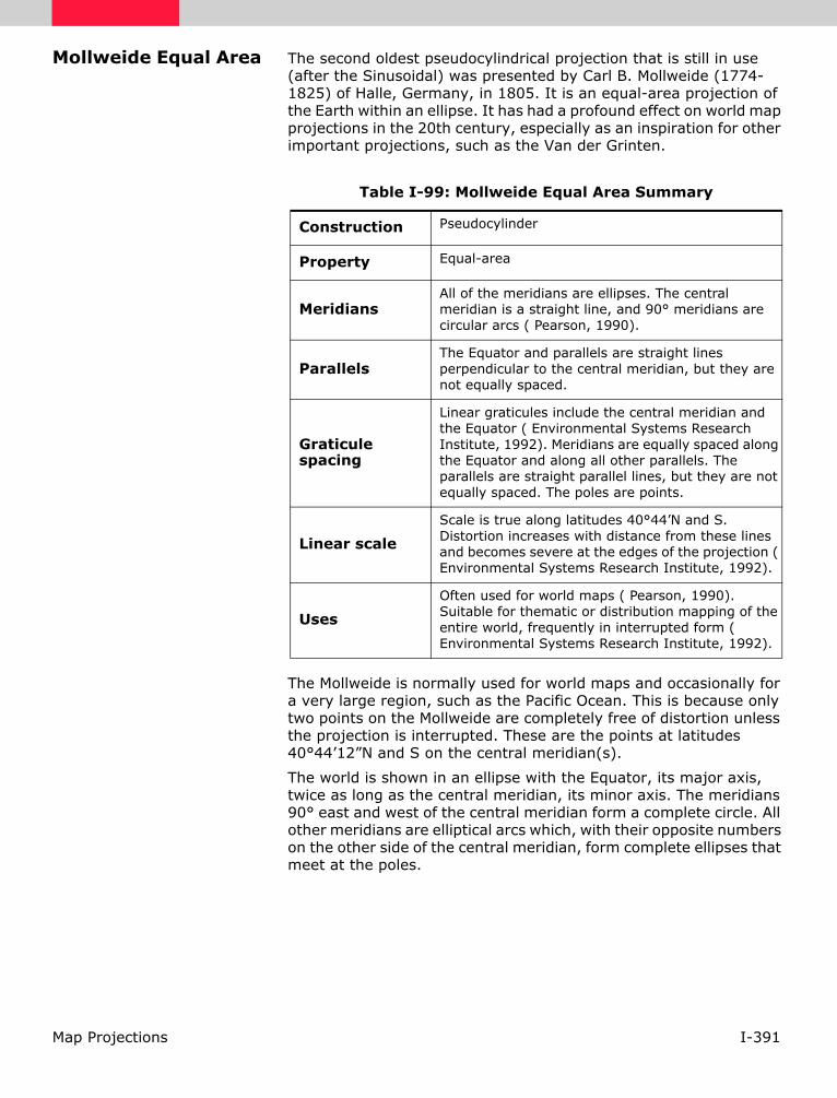
I-391Map Projections

Mollweide Equal Area The second oldest pseudocylindrical projection that is still in use (after the Sinusoidal) was presented by Carl B. Mollweide (1774-1825) of Halle, Germany, in 1805. It is an equal-area projection of the Earth within an ellipse. It has had a profound effect on world map projections in the 20th century, especially as an inspiration for other important projections, such as the Van der Grinten.

The Mollweide is normally used for world maps and occasionally for a very large region, such as the Pacific Ocean. This is because only two points on the Mollweide are completely free of distortion unless the projection is interrupted. These are the points at latitudes 40°44’12”N and S on the central meridian(s).

The world is shown in an ellipse with the Equator, its major axis, twice as long as the central meridian, its minor axis. The meridians 90° east and west of the central meridian form a complete circle. All other meridians are elliptical arcs which, with their opposite numbers on the other side of the central meridian, form complete ellipses that meet at the poles.

Table I-99: Mollweide Equal Area Summary

Construction Pseudocylinder

Property Equal-area

MeridiansAll of the meridians are ellipses. The central meridian is a straight line, and 90° meridians are circular arcs ( Pearson, 1990).

ParallelsThe Equator and parallels are straight lines perpendicular to the central meridian, but they are not equally spaced.

Graticule spacing

Linear graticules include the central meridian and the Equator ( Environmental Systems Research Institute, 1992). Meridians are equally spaced along the Equator and along all other parallels. The parallels are straight parallel lines, but they are not equally spaced. The poles are points.

Linear scale

Scale is true along latitudes 40°44’N and S. Distortion increases with distance from these lines and becomes severe at the edges of the projection ( Environmental Systems Research Institute, 1992).

Uses

Often used for world maps ( Pearson, 1990). Suitable for thematic or distribution mapping of the entire world, frequently in interrupted form ( Environmental Systems Research Institute, 1992).

I-392 Map Projections

PromptsThe following prompts display in the Projection Chooser if Mollweide Equal Area is selected.

Projection Name

Spheroid Type

Datum Name

I-393Map Projections

Rectified Skew Orthomorphic

Martin Hotine (1898 - 1968) called the Oblique Mercator projection the Rectified Skew Orthomorphic projection.

See "Oblique Mercator (Hotine)" on page I-331 for more information.

PromptsThe following prompts display in the Projection Chooser if Rectified Skew Orthomorphic is selected.

Projection Name

Spheroid Type

Datum Name

I-394 Map Projections

Robinson Pseudocylindrical

The Robinson Pseudocylindrical projection provides a means of showing the entire Earth in an uninterrupted form. The continents appear as units and are in relatively correct size and location. Poles are represented as lines.

Meridians are equally spaced and resemble elliptical arcs, concave toward the central meridian. The central meridian is a straight line 0.51 times the length of the Equator. Parallels are equally spaced straight lines between 38°N and S, and then the spacing decreases beyond these limits. The poles are 0.53 times the length of the Equator. The projection is based upon tabular coordinates instead of mathematical formulas ( Environmental Systems Research Institute, 1992).

PromptsThe following prompts display in the Projection Chooser if Robinson Pseudocylindrical is selected.

Projection Name

Spheroid Type

Datum Name

Table I-100: Robinson Pseudocylindrical Summary

Construction Pseudocylinder

Property Compromise

Meridians Meridians are elliptical arcs, equally spaced, and concave toward the central meridian.

Parallels Parallels are straight lines.

Graticule spacing

Parallels are straight lines and are parallel. The individual parallels are evenly divided by the meridians ( Pearson, 1990).

Linear scale

Generally, scale is made true along latitudes 38°N and S. Scale is constant along any given latitude, and for the latitude of opposite sign ( Environmental Systems Research Institute, 1992).

Uses

Developed for use in general and thematic world maps. Used by Rand McNally since the 1960s and by the National Geographic Society since 1988 for general and thematic world maps ( Environmental Systems Research Institute, 1992).

I-395Map Projections

Southern Orientated Gauss Conformal

Southern Orientated Gauss Conformal is another name for the Transverse Mercator projection, after mathematician Friedrich Gauss (1777-1855). It is also called the Gauss-Krüger projection.

See "Transverse Mercator" on page I-367 for more information.

PromptsThe following prompts display in the Projection Chooser if Southern Orientated Gauss Conformal is selected.

Projection Name

Spheroid Type

Datum Name

I-396 Map Projections

Swiss Cylindrical The Swiss Cylindrical projection is a cylindrical projection used by the Swiss Landestopographie, which is a form of the Oblique Mercator projection.

For more information, see "Oblique Mercator (Hotine)" on page I-331.

I-397Map Projections

Winkel’s Tripel Winkel’s Tripel was formulated in 1921 by Oswald Winkel of Germany. It is a combined projection that is the arithmetic mean of the Plate Carrée and Aitoff’s projection ( Maling, 1992).

PromptsThe following prompts display in the Projection Chooser if Winkel’s Tripel is selected.

Projection Name

Spheroid Type

Datum Name

Figure I-131: Winkel’s Tripel Projection

Source: Snyder and Voxland, 1989

Table I-101: Winkel’s Tripel Summary

Construction Modified azimuthal

Property Neither conformal nor equal-area

MeridiansCentral meridian is straight. Other meridians are curved and are equally spaced along the Equator, and concave toward the central meridian.

ParallelsEquidistant spacing of parallels. Equator and the poles are straight. Other parallels are curved and concave toward the nearest pole.

Graticule spacing

Symmetry is maintained along the central meridian or the Equator.

Linear scale Scale is true along the central meridian and constant along the Equator.

Uses Used for world maps.

I-398 Map Projections

I-399Index

IndexSymbols.OV1 (overview image) I-96.OVR (overview image) I-96.stk (GRID Stack file) I-107

Numerics1:24,000 scale I-981:250,000 scale I-992D affine transformation II-1634 mm tape I-21, I-227.5-minute DEM I-988 mm tape I-21, I-239-track tape I-21, I-23

Aa priori I-224, II-104Absorption I-7, I-10

spectra I-6, I-11Absorption spectra II-55Accuracy assessment II-142, II-145Accuracy report II-147Active sensor I-6Adaptive filter II-36Additional Parameter modeling (AP) II-193ADRG I-23, I-50, I-86

file naming convention I-91ordering I-104

ADRI I-50, I-92file naming convention I-94ordering I-104

Aerial photography I-86Aerial photos I-4, I-26, II-150Aerial triangulation (AT) II-153, II-171Airborne GPS II-170Airborne imagery I-49Airborne Imaging Spectrometer I-12Airborne Multispectral Scanner Mk2 I-12AIRSAR I-75, I-83Aitoff I-397Albers Conical Equal Area I-269, I-315Almaz I-75Almaz 1-B I-77Almaz-1 I-77Analog photogrammetry II-149Analytical photogrammetry II-149Annotation I-54, I-133, I-138, I-187

element I-187in script models I-174layer I-187

ANT (Erdas 7.x) (annotation) I-54AP II-193Arc Coverage I-50Arc Interchange (raster) I-50Arc Interchange (vector) I-55ARC system I-87, I-95Arc/second format I-97Arc_Interchange to Coverage I-55Arc_Interchange to Grid I-55ARCGEN I-50, I-55, I-112ArcInfo I-49, I-50, I-107, I-112, I-147, I-152,I-221

coverages I-35data model I-35, I-37UNGENERATE I-112

ArcInfo GENERATE I-44ArcInfo INTERCHANGE I-44ArcView I-44Area based matching II-182Area of interest I-31, I-157, II-27ASCII I-99, I-154ASCII Raster I-50ASCII To Point Annotation (annotation) I-54ASCII To Point Coverage (vector) I-55Aspect I-200, II-197, II-201

calculating II-201equatorial I-201oblique I-201polar I-201transverse I-202

ASTER I-50AT II-171Atmospheric correction II-27Atmospheric effect II-17Atmospheric modeling II-18Attribute

imported I-39in model I-172information I-35, I-37, I-39raster I-153thematic I-152vector I-152, I-154viewing I-154

Auto update I-122, I-123, I-124AutoCAD I-44, I-49, I-112Automatic image correlation II-220Automatic tie point collection II-180Average II-247AVHRR I-15, I-50, I-58, I-67, I-224, II-18, II-57

extract I-68full set I-68ordering I-103

AVHRR (Dundee Format) I-50

I-400 Index

AVHRR (NOAA) I-50AVIRIS I-11, I-83, I-84Azimuth I-199Azimuthal Equidistant I-272

BBand I-2, I-61, I-62, I-67, I-70

displaying I-126Banding I-18, II-16

see also stripingBartlett window II-75Basic Image Interchange Format I-53Bayesian classifier II-125Beam mode selection II-216Behrmann I-275BIL I-19, I-50Bin II-25Binary format I-18BIP I-19, I-21, I-50Bipolar Oblique Conic Conformal I-384Bit I-18

display device I-118in files (depth) I-16, I-18, I-22

Block of images II-179Block triangulation II-153, II-171Blocking factor I-20, I-22Bonne I-277Border I-192Bpi I-23Brightness inversion II-28Brightness value I-16, I-118, I-119, I-126, I-130, II-19Brovey Transform II-36BSQ I-19, I-50Buffer zone I-157Bundle block adjustment II-153, II-170Butterworth window II-76Byte I-18

CCADRG (Compressed ADRG) I-50Canadian Geographic Information System I-145Cartesian coordinate I-36Cartography I-183Cartridge tape I-21, I-23Cassini I-279, I-385Cassini-Soldner I-385Categorical

data I-3CCD II-186CD-ROM I-18, I-21, I-23Cell I-99

Change detection I-17, I-30, I-56, I-221Chi-square

distribution II-143statistics II-145

CIB I-96CIB (Controlled Image Base) I-50Class I-150, II-99

name I-151, I-153value I-130, I-153

numbering systems I-150, I-162Classical aerial triangulation II-153Classification I-31, I-77, I-151, II-83, II-99

and enhanced data II-45, II-103and rectified data I-222and terrain analysis II-197evaluating II-142flow chart II-129iterative II-102, II-107, II-126scheme II-102

Clump I-158Clustering II-111

ISODATA II-111, II-112RGB II-111, II-116

Coefficient II-255in convolution II-29of variation II-84

Collinearity condition II-168Collinearity equations II-172, II-192Color gun I-118, I-119, I-126Color scheme I-40, I-151Color table I-130, I-153

for printing I-260Colorcell I-120

read-only I-120Color-infrared I-125Colormap I-119, I-133Complex image I-55Confidence level II-145Conformality I-199Contiguity analysis I-156Contingency matrix II-120, II-122Continuous

data I-3Continuous data

see dataContrast stretch I-31, II-19

for display I-126, II-22, II-249linear II-20min/max vs. standard deviation I-128, II-

23nonlinear II-21piecewise linear II-21

Contrast table I-126Control point extension II-153

Index I-401

Controlled Image Base I-96Convergence value II-175Convolution I-18

cubic I-247filtering I-159, I-247, I-248, II-29kernel

crisp II-34edge detector II-32edge enhancer II-33gradient II-89high frequency II-31, II-32low frequency I-247, II-33Prewitt II-88zero-sum II-32

Convolution kernel II-29high frequency I-248low frequency I-248Prewitt II-89

CoordinateCartesian I-36, I-203conversion I-252file I-3, I-36, I-142geographic I-203, I-303map I-4, I-36, I-219, I-222, I-223planar I-203reference I-222, I-223retransformed I-244source I-223spherical I-203

Coordinate system I-3, II-157ground space II-157image space II-157

Correlation calculations II-182Correlation coefficient II-224Correlation threshold I-225Correlation windows II-182Correlator library II-224Covariance II-123, II-135, II-250

sample II-250Covariance matrix II-48, II-119, II-124, II-137, II-251Cross correlation II-182

DDAEDALUS I-50, I-84DAEDALUS TMS

bands/frequencies I-84Data I-146

airborne sensor I-49ancillary II-104categorical I-3complex I-55compression II-46, II-116

continuous I-3, I-24, I-125, I-149displaying I-129

creating I-143elevation II-104, II-197enhancement II-12from aircraft I-83geocoded I-20, I-29, I-220gray scale I-139hyperspectral I-11interval I-3nominal I-3ordering I-103ordinal I-3packed I-67pseudo color I-138radar I-49, I-72

applications I-76bands I-75merging II-96

raster I-3, I-133converting to vector I-106editing I-31formats (BIL, etc.) I-22importing and exporting I-50in GIS I-148sources I-49

ratio I-3satellite I-49structure II-50thematic I-3, I-24, I-130, I-151, II-107

displaying I-132tiled I-26, I-55topographic I-97, II-197

using I-99true color I-139vector I-133, I-138, I-152, I-221, I-253

converting to raster I-106, I-151copying I-39displaying I-40editing I-177

densify I-178generalize I-178reshape I-178spline I-177split I-178unsplit I-178

from raster data I-42importing I-42, I-55in GIS I-148renaming I-39sources I-42, I-44, I-49structure I-37

viewing I-138multiple layers I-139

I-402 Index

overlapping layers I-139Data correction I-17, I-31, II-11, II-15

geometric I-219, II-15, II-18radiometric I-220, II-15, II-93

Data file value I-1, I-31display I-126, I-142, II-20in classification II-99

Data storage I-18Database

image I-28Decision rule II-101, II-127

Bayesian II-137feature space II-132Mahalanobis distance II-135maximum likelihood II-136, II-143minimum distance II-133, II-136, II-143,

II-145non-parametric II-127parallelepiped II-129parametric II-128

Decision tree II-141Decorrelation stretch II-50Degrees of freedom II-145DEM I-2, I-26, I-97, I-98, I-220, II-18, II-198

editing I-32interpolation I-32ordering I-103

Density I-23Density of detail II-225Descriptive information

see attribute information I-39Desktop Scanners I-85Desktop scanners II-155Detector I-57, II-15DFAD I-55DGN I-44DGN (Intergraph IGDS) (vector) I-55Differential collection geometry II-233Differential correction I-101DIG Files (Erdas 7.x) (vector) I-55Digital image I-42Digital orthophoto II-194Digital orthophotography II-198Digital photogrammetry II-150Digital picture

see image I-118Digital terrain model (DTM) I-49Digitizing I-42, I-221

GCPs I-224operation modes I-43point mode I-43screen I-42, I-44stream mode I-43tablet I-42

DIME I-114Dimensionality II-46, II-103, II-104, II-254Direction of flight II-154Discrete Cosine Transformation I-107Disk space I-23Diskette I-18, I-21Display

32-bit I-121DirectColor I-121, I-122, I-128, I-131HiColor I-121, I-124PC I-125PseudoColor I-121, I-124, I-129, I-132TrueColor I-121, I-123, I-124, I-128, I-

131Display device I-117, I-126, II-19, II-22, II-52Display memory II-12Display resolution I-117Distance image file II-143, II-144Distribution II-244Distribution Rectangle I-87Dithering I-137

color artifacts I-138color patch I-137

Divergence II-120signature II-123transformed II-124

DLG I-23, I-44, I-49, I-55, I-113Doppler centroid II-212Doppler cone II-212DOQ I-50DOQ (JPEG) I-50DOQs I-86DTED I-50, I-92, I-97, II-198DTM I-49DXF I-44, I-49, I-54, I-112DXF to Annotation I-56DXF to Coverage I-56Dynamic range I-16

EEarth Centered System II-211Earth Fixed Body coordinate system II-210Earth model II-212Eckert I I-281Eckert II I-283Eckert III I-285Eckert IV I-287Eckert V I-289Eckert VI I-291Edge detection II-32, II-87Edge enhancement II-33Eigenvalue II-46

Index I-403

Eigenvector II-46, II-48Eikonix I-85Electric field II-227Electromagnetic radiation I-5, I-57Electromagnetic spectrum I-2, I-5

long wave infrared region I-5short wave infrared region I-5

Electromagnetic wave II-226, II-238Elements of exterior orientation II-165Ellipse II-46, II-120Ellipsoid II-217Enhancement I-30, I-64, II-11, II-99

linear I-127, II-20nonlinear II-20on display I-133, I-142, II-12radar data II-11, II-80radiometric II-11, II-18, II-28spatial II-11, II-18, II-28spectral II-11, II-45

Entity (AutoCAD) I-113EOF (end of file) I-20EOSAT I-17, I-29, I-61, I-103EOSAT SOM I-293EOV (end of volume) I-20Ephemeris adjustment II-213Ephemeris coordinate system II-210Ephemeris data II-189Ephemeris modeling II-210equal area

see equivalenceEquidistance I-199Equidistant Conic I-294, I-325Equidistant Cylindrical I-296, I-385Equirectangular I-297Equivalence I-199ER Mapper I-50ERDAS macro language (EML) I-156ERDAS Version 7.X I-25, I-106EROS Data Center I-104Error matrix II-147ERS (Conae-PAF CEOS) I-51ERS (D-PAF CEOS) I-51ERS (I-PAF CEOS) I-51ERS (Tel Aviv-PAF CEOS) I-51ERS (UK-PAF CEOS) I-51ERS-1 I-75, I-77, I-78

ordering I-105ERS-2 I-77, I-79ESRI I-35, I-145ETAK I-44, I-49, I-56, I-114Euclidean distance II-134, II-143, II-255Expected value II-248Expert classification II-139Exposure station II-154

Extent I-188Exterior orientation II-165

SPOT II-188

F.fsp.img file II-108False color I-64False easting I-203False northing I-203Fast format I-20Fast Fourier Transform II-66Feature based matching II-184Feature extraction II-11Feature point matching II-184Feature space II-253

area of interest II-105, II-109image II-108, II-253

Fiducial marks II-162Field I-152File

.fsp.img II-108

.gcc I-224

.GIS I-25, I-106

.gmd I-168

.img I-2, I-24, I-125

.LAN I-25, I-106

.mdl I-174

.ovr I-187

.sig II-250archiving I-29header I-22output I-24, I-28, I-173, I-241, I-242

.img II-22classification II-101

pixel I-118tic I-36

File coordinate I-3File name I-28Film recorder I-259Filter

adaptive II-36Fourier image II-72Frost II-81, II-86Gamma-MAP II-81, II-86high-pass II-74homomorphic II-78Lee II-81, II-83Lee-Sigma II-80local region II-80, II-82low-pass II-72mean II-80, II-81median I-18, II-80, II-81, II-82periodic noise removal II-77

I-404 Index

Sigma II-83zero-sum II-89

Filtering II-30see also convolution filtering

FIT I-51Flattening II-237Flight path II-154Focal analysis I-18Focal length II-162Focal operation I-31, I-159Focal plane II-162Fourier analysis II-11, II-66Fourier magnitude II-66

calculating II-68Fourier Transform

calculation II-67Editor

window functions II-74filtering II-72high-pass filtering II-74inverse

calculating II-71low-pass filtering II-72neighborhood techniques II-65noise removal II-77point techniques II-65

Frequencystatistical II-244

Frost filter II-81, II-86Function memory II-12Fuyo 1 I-75

ordering I-105Fuzzy convolution II-138Fuzzy methodology II-138

G.gcc file I-224.GIS file I-25, I-106.gmd file I-168GAC (Global Area Coverage) I-67Gamma-MAP filter II-81, II-86Gauss Kruger I-300Gaussian distribution II-85Gauss-Krüger I-395GCP I-223, II-256

corresponding I-223digitizing I-224matching I-224, I-225minimum required I-235prediction I-224, I-225selecting I-223

GCP configuration II-179GCP requirements II-178

GCPs II-177General Vertical Near-side Perspective I-301Generic Binary I-51Geocentric coordinate system II-159Geocoded data I-20Geocoding

GeoTIFF I-111Geographic Information System

see GISGeoid II-217Geology I-77Georeference I-220, I-255Georeferencing

GeoTIFF I-111GeoTIFF I-51, I-111

geocoding I-111georeferencing I-111

Gigabyte I-18GIS I-1

database I-147defined I-146history I-145

GIS (Erdas 7.x) I-51Glaciology I-77Global operation I-31GLONASS I-100Gnomonic I-305GOME I-79GPS data I-100GPS data applications I-101GPS satellite position I-100Gradient kernel II-89Graphical model I-155, II-12

convert to script I-174create I-168

Graphical modeling I-157, I-166GRASS I-51Graticule I-193, I-203Gray scale II-198Gray values II-194GRD I-51Great circle I-199GRID I-51, I-106, I-107GRID (Surfer

ASCII/Binary) I-51Grid cell I-1, I-118Grid line I-192GRID Stack I-51GRID Stack7x I-51GRID Stacks I-107Ground Control Point

see GCPGround coordinate system II-159Ground space II-157

Index I-405

Ground truth II-99, II-105, II-106, II-120Ground truth data I-101Ground-based photographs II-150

HHalftone I-259Hammer I-307Hardcopy I-255Hardware I-117HD II-222Header

file I-20, I-22record I-20

HFA file II-217Hierarchical pyramid technique II-221High density (HD) II-222High Resolution Visible sensors (HRV) II-186Histogram I-151, I-153, II-19, II-116, II-243,II-244, II-253, II-254

breakpoint II-23signature II-120, II-126

Histogram equalizationformula II-26

Histogram match II-27Homomorphic filtering II-78Host workstation I-117Hotine I-331HRPT (High Resolution Picture Transmission)I-67HRV II-186Hue II-52Huffman encoding I-107Hydrology I-77Hyperspectral data I-11Hyperspectral image processing II-11

I.img file I-2, I-24Ideal window II-75IFOV (instantaneous field of view) I-15IGDS I-56IGES I-44, I-49, I-56, I-115IHS to RGB II-54IKONOS I-58

bands/frequencies I-59Image I-1, I-118, II-11

airborne I-49complex I-55digital I-42microscopic I-49pseudo color I-40radar I-49raster I-42

ungeoreferenced I-36Image algebra II-57, II-103Image Catalog I-27, I-29Image coordinate system II-158Image data I-1Image display I-2, I-117Image file I-1, I-125, II-198

statistics II-243Image Information I-127, I-135, I-152, I-220,I-222Image Interpreter I-11, I-18, I-151, I-154, I-155, II-12, II-22, II-35, II-36, II-51, II-93, II-116, II-199, II-201, II-204, II-205

functions II-13Image processing I-1Image pyramid II-185Image registration II-234Image scale (SI) II-154, II-195Image space II-157, II-162Image space coordinate system II-158IMAGINE Developers’ Toolkit I-156, I-213, I-263IMAGINE Expert Classifier II-139IMAGINE OrthoRadar algorithm description II-210IMAGINE Radar Interpreter II-80IMAGINE StereoSAR DEM

Constraintheory II-220

Degradetheory II-219, II-225

Despeckletheory II-218

Heighttheory II-225

Inputtheory II-216

Matchtheory II-220

Registertheory II-219

Rescaletheory II-219

Subsettheory II-218

IMAGINE StereoSAR DEM process flow II-215Import

direct I-50generic I-55

Incidence angles II-189Inclination II-190Inclination angles II-189Index I-157, I-163, II-55

application II-56

I-406 Index

vegetation I-11Inertial navigation system I-102INFO I-39, I-113, I-114, I-115, I-153

path I-40see also ArcInfo

Information (vs. data) I-146INS II-170Intensity II-52Interferometric model II-229Interior orientation II-161

SPOT II-187International Dateline I-203Interpretative photogrammetry II-150Interrupted Goode Homolosine I-309Interrupted Mollweide I-311Interval

classes I-150, I-244data I-3

IRS I-59IRS-1C I-59IRS-1C (EOSAT Fast Format C) I-51IRS-1C (EUROMAP Fast Format C) I-51IRS-1C/1D I-51IRS-1D I-60

JJeffries-Matusita distance II-124JERS-1 I-77, I-79

bands/frequencies I-80ordering I-105

JFIF (JPEG) I-51, I-107JPEG File Interchange Format I-107

KKappa II-166Kappa coefficient II-147Knowledge Classifier II-142Knowledge Engineer II-140Kurtosis II-92

L.LAN file I-25, I-106Laborde Oblique Mercator I-387LAC (Local Area Coverage) I-67Lambert Azimuthal Equal Area I-312Lambert Conformal I-353Lambert Conformal Conic I-315, I-384, I-389Lambertian reflectance model II-205LAN (Erdas 7.x) I-51Landsat I-10, I-17, I-26, I-42, I-51, I-57, I-58, I-350, II-11, II-18, II-36

description I-57, I-61history I-61

MSS I-15, I-61, I-62, II-16, II-18, II-57ordering I-103TM I-9, I-10, I-14, I-20, I-62, I-222, I-

224, II-34, II-54, II-57, II-82, II-98

displaying I-126Landsat 7 I-65

characteristics I-65data types I-65

Laplacian operator II-88, II-90Latitude/Longitude I-97, I-203, I-220, I-303

rectifying I-243Layer I-2, I-149, I-166Least squares adjustment II-173Least squares condition II-174Least squares correlation II-183Least squares regression I-227, I-231Lee filter II-81, II-83Lee-Sigma filter II-80Legend I-192Lens distortion II-164Level 1B data I-227Level slice II-27Light SAR I-83Line I-36, I-41, I-55, I-114Line detection II-87Line dropout I-18, II-16Linear regression II-17Linear transformation I-227, I-231Lines of constant range II-95LISS-III I-59

bands/frequencies I-59Local region filter II-80, II-82Long wave infrared region I-5Lookup table I-119, II-19

display II-23Low parallax (LP) II-222Lowtran I-9, II-18Loximuthal I-318LP II-222

M.mdl file I-174Magnification I-118, I-140, I-141Magnitude of parallax II-224Mahalanobis distance II-143Map I-183

accuracy I-210, I-217aspect I-184base I-184bathymetric I-184book I-255cadastral I-184

Index I-407

choropleth I-184colors in I-186composite I-184composition I-216contour I-184credit I-195derivative I-184hardcopy I-218index I-184inset I-184isarithmic I-184isopleth I-184label I-194land cover II-99lettering I-196morphometric I-184outline I-184output to TIFF I-258paneled I-255planimetric I-72, I-184printing I-255

continuous tone I-260with black ink I-261

qualitative I-185quantitative I-185relief I-184scale I-210, I-256scaled I-255, I-259shaded relief I-184slope I-184thematic I-185title I-195topographic I-72, I-185typography I-195viewshed I-185

Map Composer I-183, I-257Map coordinate I-4, I-222, I-223

conversion I-252Map projection I-198, I-219, I-221, I-263

azimuthal I-198, I-200, I-210compromise I-198conformal I-211conical I-198, I-201, I-210cylindrical I-198, I-201, I-210equal area I-211external I-205, I-382gnomonic I-201modified I-202orthographic I-201planar I-198, I-200pseudo I-202see also specific projectionselecting I-210stereographic I-201

types I-200units I-207USGS I-203, I-264

MapBasesee ETAK

Mapping I-183Mask I-160Matrix II-257

analysis I-157, I-165contingency II-120, II-122covariance II-48, II-119, II-124, II-137,

II-251error II-147transformation I-222, I-224, I-241, II-256

Matrix algebraand transformation matrix II-257multiplication II-257notation II-257transposition II-258

Maximum likelihoodclassification decision rule II-123

Mean I-127, II-23, II-121, II-246, II-248, II-249

of ISODATA clusters II-112vector II-124, II-252

Mean Euclidean distance II-92Mean filter II-80, II-81Measurement I-43Measurement vector II-251, II-253, II-257Median filter II-80, II-81, II-82Megabyte I-18Mercator I-202, I-320, I-323, I-331, I-367, I-374, I-385Meridian I-203Metric photogrammetry II-150Microscopic imagery I-49Microsoft Windows NT I-117, I-124MIF/MID (MapInfo) to Coverage I-56Miller Cylindrical I-323Minimum distance

classification decision rule II-115, II-123Minimum Error Conformal I-388Minnaert constant II-206Model I-166, I-167Model Maker I-155, I-166, II-12

criteria function I-172functions I-169object I-170

data type I-171matrix I-171raster I-170scalar I-171table I-171

working window I-172

I-408 Index

Modeling I-31, I-165and image processing I-166and terrain analysis II-197using conditional statements I-172

Modified Polyconic I-389Modified Stereographic I-390Modified Transverse Mercator I-325MODIS I-51Modtran I-9, II-18Mollweide I-327Mollweide Equal Area I-391Mosaic I-29, I-30, I-221MrSID I-51, I-108MSS Landsat I-51Multiplicative algorithm II-35Multispectral imagery I-57, I-70Multitemporal imagery I-30

NNadir I-57, II-189NASA I-61, I-73, I-83NASA ER-2 I-84NASA/JPL I-83NASDA CEOS I-51Natural-color I-125NAVSTAR I-100Nearest neighbor

see resampleNeatline I-192Negative inclination II-189Neighborhood analysis I-157, I-159

boundary I-160density I-160diversity I-160majority I-160maximum I-160mean I-160median I-161minimum I-161minority I-161rank I-161standard deviation I-161sum I-161

New Zealand Map Grid I-329NITFS I-53NLAPS I-51, I-66NOAA I-67Node I-36

dangling I-181from-node I-36pseudo I-181to-node I-36

Noise reduction II-236

Noise removal II-77Nominal

classes I-150, I-244data I-3

Non-Lambertian reflectance model II-205, II-206Nonlinear transformation I-229, I-232, I-234Normal distribution II-46, II-135, II-136, II-137, II-246, II-247, II-250, II-254Normalized correlation coefficient II-224Normalized Difference Vegetation Index (ND-VI) I-11, II-57, II-58

O.OV1 (overview image) I-96.OVR (overview image) I-96.ovr file I-187Oblated Equal Area I-330Oblique Mercator I-331, I-353, I-387, I-393Oblique photographs II-150Observation equations II-172Oceanography I-77Off-nadir I-70, II-189Offset I-227Oil exploration I-77Omega II-166Opacity I-139, I-153Optical disk I-21Orb View-3

bands/frequencies I-69Orbit correction II-217OrbView3 I-68Order

of polynomial II-255of transformation II-256

Ordinalclasses I-150, I-244data I-3

Orientation II-166Orientation angle II-191Orthocorrection I-99, I-220, II-18, II-95Orthographic I-334Orthorectification I-220, II-193, II-214Output file I-24, I-173, I-241, I-242

.img II-22classification II-101

Output formation II-214Overlay I-157, I-162Overlay file I-187Overview images I-96

PPanchromatic

Index I-409

band/frequency I-60Panchromatic imagery I-57, I-70Panchromatic sensor I-59Parallax II-223Parallel I-203Parallelepiped

alarm II-120Parameter II-249Parametric II-136, II-137, II-250Passive sensor I-6Pattern recognition II-99, II-120PCX I-51Periodic noise removal II-77Phase II-236, II-237, II-238, II-240Phase function II-239Phi II-166Photogrammetric configuration II-171Photogrammetric scanners I-85, II-155Photogrammetry II-149Photograph I-49, I-56, II-36

aerial I-83ordering I-104

Pixel I-1, I-118depth I-117display I-118file vs. display I-118

Pixel coordinate system II-157, II-162Plane table photogrammetry II-149Plate Carrée I-297, I-337, I-385, I-397Point I-35, I-41, I-55, I-114

label I-36Point ID I-223Polar Stereographic I-338, I-389Pollution monitoring I-77Polyconic I-325, I-341, I-389Polygon I-36, I-41, I-55, I-114, I-159, I-177,II-62, II-105Polynomial I-230, II-255Positive inclination II-189Posting II-224PostScript I-257Preference Editor I-134Prewitt kernel II-88, II-89Primary color I-118, I-261

RGB vs. CMY I-261Principal component band II-47Principal components I-31, II-34, II-35, II-46,II-50, II-103, II-251, II-254

computing II-48Principal point II-162Printer

PostScript I-257Tektronix Inkjet I-259Tektronix Phaser I-259

Tektronix Phaser II SD I-260Probability II-126, II-136Processing a strip of images II-178Processing one image II-178Profile I-97Projection

externalBipolar Oblique Conic Conformal I-384Cassini-Soldner I-385Laborde Oblique Mercator I-387Modified Polyconic I-389Modified Stereographic I-390Mollweide Equal Area I-391Rectified Skew Orthomorphic I-393Robinson Pseudocylindrical I-394Southern Orientated Gauss Conformal

I-395Winkel’s Tripel I-397

perspective I-363USGS

Alaska Conformal I-267Albers Conical Equal Area I-269Azimuthal Equidistant I-272Bonne I-277Cassini I-279Conic Equidistant I-294Eckert IV I-287Eckert VI I-291Equirectangular (Plate Carrée) I-297Gall Stereographic

Gall Stereographic I-299General Vertical Nearside Perspective

I-301Geographic (Lat/Lon) I-303Gnomonic I-305Hammer I-307Lambert Azimuthal Equal Area I-312Lambert Conformal Conic I-315Mercator I-320Miller Cylindrical I-323Modified Transverse Mercator I-325Mollweide I-327Oblique Mercator (Hotine) I-331Orthographic I-334Polar Stereographic I-338Polyconic I-341Sinusoidal I-348Space Oblique Mercator I-350State Plane I-353Stereographic I-363Transverse Mercator I-367Two Point Equidistant I-369UTM I-371Van der Grinten I I-374

I-410 Index

Projection Chooser I-203Proximity analysis I-156Pseudo color I-64

display I-150Pseudo color image I-40Pushbroom scanner I-70Pyramid layer I-27, I-134Pyramid technique II-221Pythagorean Theorem II-255

QQuartic Authalic I-343Quick tests II-225

RRadar I-4, I-18, II-36, II-89, II-90, II-91Radar imagery I-49RADARSAT I-51, I-77, I-80

beam mode resolution I-80ordering I-105

RADARSAT (Acres CEOS) I-51RADARSAT (Vancouver CEOS) I-51RADARSAT Beam mode II-224Radial lens distortion II-164Radiative transfer equation I-9RAM I-133Range line II-94Range sphere II-212Raster

data I-3Raster Attribute Editor I-131, I-154Raster editing I-31Raster image I-42Raster Product Format I-52, I-95Raster region I-158Ratio

classes I-150, I-244data I-3

Rayleigh scattering I-8Real time differential GPS I-101Recode I-31, I-157, I-161, I-166Record I-22, I-152

logical I-22physical I-22

Rectification I-29, I-219process I-222

Rectified Skew Orthomorphic I-393Reduction I-141Reference coordinate I-222, I-223Reference pixel II-146Reference plane II-160Refined ephemeris II-218Reflect I-227, I-228

Reflection spectra I-6see absorption spectra

Registration I-219vs. rectification I-222

Relation based matching II-184Remote sensing I-219Report

generate I-154Resample I-219, I-222, I-241

Bicubic Spline I-242Bilinear Interpolation I-133, I-242, I-244Cubic Convolution I-134, I-242, I-247for display I-133Nearest Neighbor I-133, I-242, I-243, I-

247Residuals I-238Resolution I-14, II-156

display I-117merge II-34radiometric I-14, I-16, I-17, I-61spatial I-15, I-17, I-256, II-27spectral I-14, I-17temporal I-14, I-17

Resolution mergeBrovey Transform II-36Multiplicative II-35Principal Components Merge II-35

Retransformed coordinate I-244RGB monitor I-119RGB to IHS II-97Rhumb line I-199Right hand rule II-159RMS error I-224, I-227, I-238, I-240, II-163

tolerance I-240total I-239

RMSE II-155Roam I-141Robinson I-345Robinson Pseudocylindrical I-394Root mean square error II-163Root Mean Square Error (RMSE) II-155Rotate I-227Rotation matrix II-166RPF I-95RPF Cell I-96RPF Frame I-96RPF Overview I-96RPF Product I-96RSO I-347Rubber sheeting I-229

S.sig file II-250

Index I-411

.stk (GRID Stack file) I-107Sanson-Flamsteed I-348SAR I-73SAR image intersection II-216SAR imaging model II-211Satellite I-56

imagery I-4system I-56

Satellite photogrammetry II-185Satellite scene II-187Saturation II-52Scale I-15, I-188, I-227, I-255

display I-256equivalents I-189large I-15map I-256paper I-257

determining I-258pixels per inch I-189representative fraction I-188small I-15verbal statement I-188

Scale bar I-188Scaled map I-259Scan line II-186Scanner I-57Scanners I-85Scanning I-84, I-221Scanning resolutions II-156Scanning window I-159Scattering I-7

Rayleigh I-8Scatterplot II-46, II-116, II-254

feature space II-108SCBA II-193Screendump command I-109Script model I-155, II-12

data type I-177library I-174statement I-176

Script modeling I-157SDE I-52SDTS I-45, I-108SDTS (raster) I-52SDTS (vector) I-56SDTS profiles I-108SDTS Raster Profile and Extensions I-108Search area II-220, II-223Seasat-1 I-73Seat I-117SeaWiFS I-69

bands/frequencies I-69SeaWiFS L1B and L2A I-52Secant I-201

Seed properties II-106Self-calibrating bundle adjustment (SCBA) II-193Sensor I-57

active I-6, I-74passive I-6, I-74radar I-77

Separabilitylisting II-125signature II-123

Shaded relief II-197, II-203calculating II-204

Shadowenhancing II-21

Shapefile I-52Ship monitoring I-77Short wave infrared region I-5SI II-195Sigma filter II-83Sigma notation II-243Signal based matching II-182Signature II-100, II-101, II-104, II-107, II-118

alarm II-120append II-126contingency matrix II-122delete II-126divergence II-120, II-123ellipse II-120, II-121evaluating II-119file II-250histogram II-120, II-126manipulating II-107, II-126merge II-126non-parametric II-100, II-109, II-119parametric II-100, II-119separability II-123, II-125statistics II-120, II-126transformed divergence II-124

Simple Conic I-294Simple Cylindrical I-297Single frame orthorectification II-152Sinusoidal I-202, I-348SIR-A I-75, I-77, I-81

ordering I-105SIR-B I-75, I-77, I-81

ordering I-105SIR-C I-77, I-82

ordering I-105SIR-C/X-SAR I-82

bands/frequencies I-82Skew I-227Skewness II-92Slant range II-212

I-412 Index

Slant-to-ground range correction II-95SLAR I-73, I-75Slope II-197, II-199

calculating II-199Softcopy photogrammetry II-150Source coordinate I-223Southern Orientated Gauss Conformal I-395Space forward intersection II-169Space Oblique Mercator I-202, I-331, I-350Space Oblique Mercator (Formats A & B) I-352Space resection II-152, II-169Sparse mapping grid II-214Spatial frequency II-28Spatial Modeler I-18, I-55, I-151, I-166, II-12, II-206Spatial Modeler Language I-155, I-166, I-173,II-12Speckle noise I-76, II-80

removing II-81Speckle suppression I-18

local region filter II-82mean filter II-81median filter II-81, II-82Sigma filter II-83

Spectral dimensionality II-251Spectral distance II-123, II-133, II-143, II-145, II-255

in ISODATA clustering II-112Spectral space II-46, II-48, II-253Spectroscopy I-6Spheroid I-211, I-212SPOT I-10, I-15, I-17, I-26, I-29, I-42, I-52,I-57, I-58, I-70, I-92, I-115, I-224, II-11, II-18, II-36

ordering I-103panchromatic I-15, II-34, II-54XS I-70, II-57

displaying I-126SPOT (GeoSpot) I-52SPOT 4

bands/frequencies I-72SPOT CCRS I-52SPOT exterior orientation II-188SPOT interior orientation II-187SPOT SICORP MetroView I-52SPOT4 I-72SRPE I-108Standard Beam Mode II-222Standard deviation I-128, II-23, II-121, II-248

sample II-249Standard meridian I-199, I-202Standard parallel I-199, I-201State Plane I-207, I-212, I-316, I-353, I-367

Statistics I-27, II-243signature II-120

Step size II-224Stereographic I-338, I-363Stereographic (Extended) I-366Stereoscopic imagery I-72Striping I-18, II-48, II-82Subset I-29Summation II-243Sun angle II-203SUN Raster I-52Sun Raster I-106, I-109Surface generation

weighting function I-33Swath width I-57Swiss Cylindrical I-396Symbol I-193

abstract I-193function I-194plan I-194profile I-194replicative I-193

Symbolization I-35Symbology I-40Symmetric lens distortion II-164

TTangent I-201Tangential lens distortion II-164Tape I-18Tasseled Cap transformation II-51, II-57Tektronix

Inkjet Printer I-259Phaser II SD I-260Phaser Printer I-259

Template II-220Template size II-222Terramodel I-56Terrestrial photography II-150, II-160Texture analysis II-91Thematic

data I-3Thematic data

see dataTheme I-149Threshold II-143, II-224Thresholding II-143Thresholding (classification) II-135Tick mark I-192Tie point distribution II-180Tie points II-153, II-180TIFF I-52, I-85, I-106, I-109, I-257, I-258TIGER I-45, I-49, I-56, I-115

Index I-413

disk space requirement I-116Time II-212TM Landsat Acres Fast Format I-52TM Landsat Acres Standard Format I-52TM Landsat EOSAT Fast Format I-52TM Landsat EOSAT Standard Format I-52TM Landsat ESA Fast Format I-52TM Landsat ESA Standard Format I-52TM Landsat IRS Fast Format I-52TM Landsat IRS Standard Format I-52TM Landsat Radarsat Fast Format I-52TM Landsat Radarsat Standard Format I-52TM Landsat-7 Fast-L7A EROS I-52Topocentric coordinate system II-160Topographic effect II-204Topological Vector Profile I-108Topology I-37, I-178

constructing I-179Total field of view I-57Total RMS error I-239Training II-99

supervised II-99, II-103supervised vs. unsupervised II-103unsupervised II-100, II-103, II-111

Training field II-105Training sample I-221, II-105, II-108, II-146,II-254

defining II-106evaluating II-107

Training sitesee training field

Transformation1st-order I-227linear I-227, I-231matrix I-226, I-229nonlinear I-229, I-232, I-234order I-226

Transformation matrix I-222, I-224, I-226, I-229, I-241, II-256Transposition II-137, II-258Transposition function II-123, II-136, II-137Transverse Mercator I-325, I-353, I-367, I-371, I-385, I-395True color I-64True direction I-199Two Point Equidistant I-369Type style

on maps I-195

UUngeoreferenced image I-36Universal Polar Stereographic I-338Universal Transverse Mercator I-325, I-367,

I-371Unwrapped phase II-240Unwrapping II-238USGS DEM I-50USRP I-52UTM

see Universal Transverse Mercator

VV residual matrix II-175Van der Grinten I I-374, I-391Variable I-150

in models I-177Variable rate technology I-102Variance II-92, II-135, II-248, II-249, II-250,II-251

sample II-248Vector II-257Vector data

see dataVector layer I-37Vector Quantization I-95Vegetation index I-11, II-57Velocity vector II-191Vertex I-36Viewer I-133, I-134, I-157, II-12

dithering I-137linking I-140

Volume I-23set I-23

VPF I-45, I-56VQ I-95

WWagner IV I-376Wagner VII I-378Wavelet I-108Weight factor I-164

classificationseparability II-125

Weighting function (surfacing) I-33Wide Field Sensor I-60WiFS I-60

bands/frequencies I-60Winkel I I-380Winkel II I-380Winkel’s Tripel I-397Workspace I-38

XX matrix II-174X residual I-238X RMS error I-239

I-414 Index

X Window I-117XSCAN I-85

YY residual I-238Y RMS error I-239

ZZero-sum filter II-32, II-89Zone I-87, I-95Zone distribution rectangle (ZDR) I-87Zoom I-140, I-141