equivariant kk-theory and noncommutative index theory/brodzki... · i=1 b. kasparov stabilization...
TRANSCRIPT

Equivariant KK-theory and noncommutative index theory
Jacek Brodzki
Notes taken by
Pawe l Witkowski
April 2007

Contents
Introduction to KK-theory 4
Motivation and background . . . . . . . . . . . . . . . . . . . . . . . . . . . . . . . 4
Definition . . . . . . . . . . . . . . . . . . . . . . . . . . . . . . . . . . . . . . . . . 5
Properties . . . . . . . . . . . . . . . . . . . . . . . . . . . . . . . . . . . . . . . . . 6
Applications and further development . . . . . . . . . . . . . . . . . . . . . . . . . 7
1 C*-algebras 9
1.1 Definitions . . . . . . . . . . . . . . . . . . . . . . . . . . . . . . . . . . . . . . 9
1.2 Examples . . . . . . . . . . . . . . . . . . . . . . . . . . . . . . . . . . . . . . 9
1.3 Gelfand transform . . . . . . . . . . . . . . . . . . . . . . . . . . . . . . . . . 13
2 K-theory 16
2.1 Definitions . . . . . . . . . . . . . . . . . . . . . . . . . . . . . . . . . . . . . . 16
2.2 Unitizations and multiplier algebras . . . . . . . . . . . . . . . . . . . . . . . 17
2.3 Stabilization . . . . . . . . . . . . . . . . . . . . . . . . . . . . . . . . . . . . . 18
2.4 Higher K-theory . . . . . . . . . . . . . . . . . . . . . . . . . . . . . . . . . . 18
2.5 Excision and relative K-theory . . . . . . . . . . . . . . . . . . . . . . . . . . 19
2.6 Products . . . . . . . . . . . . . . . . . . . . . . . . . . . . . . . . . . . . . . . 21
2.7 Bott periodicity . . . . . . . . . . . . . . . . . . . . . . . . . . . . . . . . . . . 21
2.8 Cuntz’s proof of Bott periodicity . . . . . . . . . . . . . . . . . . . . . . . . . 23
2.9 The Mayer-Vietoris sequence . . . . . . . . . . . . . . . . . . . . . . . . . . . 24
3 Hilbert modules 25
3.1 Definitions . . . . . . . . . . . . . . . . . . . . . . . . . . . . . . . . . . . . . . 25
3.2 Kasparov stabilization theorem . . . . . . . . . . . . . . . . . . . . . . . . . . 29
3.3 Morita equivalence . . . . . . . . . . . . . . . . . . . . . . . . . . . . . . . . . 29
3.4 Tensor products of Hilbert modules . . . . . . . . . . . . . . . . . . . . . . . . 30
4 Fredholm modules and Kasparov’s K-homology 32
4.1 Fredholm modules . . . . . . . . . . . . . . . . . . . . . . . . . . . . . . . . . 32
4.2 Commutator conditions . . . . . . . . . . . . . . . . . . . . . . . . . . . . . . 35
4.3 Quantised calculus of one variable . . . . . . . . . . . . . . . . . . . . . . . . 37
4.4 Quantised differential calculus . . . . . . . . . . . . . . . . . . . . . . . . . . . 37
4.5 Closed graded trace . . . . . . . . . . . . . . . . . . . . . . . . . . . . . . . . 38
4.6 Index pairing formula . . . . . . . . . . . . . . . . . . . . . . . . . . . . . . . 39
4.7 Kasparov’s K-homology . . . . . . . . . . . . . . . . . . . . . . . . . . . . . . 40
2

5 Boundary maps in K-homology 43
5.1 Relative K-homology . . . . . . . . . . . . . . . . . . . . . . . . . . . . . . . . 435.2 Semisplit extensions . . . . . . . . . . . . . . . . . . . . . . . . . . . . . . . . 435.3 Schrodinger pairs . . . . . . . . . . . . . . . . . . . . . . . . . . . . . . . . . . 455.4 The index pairing . . . . . . . . . . . . . . . . . . . . . . . . . . . . . . . . . . 485.5 Product of Fredholm operators . . . . . . . . . . . . . . . . . . . . . . . . . . 53
6 Equivariant K-homology of spaces 54
7 KK-theory 57
7.1 Kasparov’s bifunctor . . . . . . . . . . . . . . . . . . . . . . . . . . . . . . . . 577.2 Equivariant KK-theory . . . . . . . . . . . . . . . . . . . . . . . . . . . . . . . 587.3 Kasparov product . . . . . . . . . . . . . . . . . . . . . . . . . . . . . . . . . 59
3

Introduction to KK-theory
Lecture given by Christian Voigt
Motivation and background
Atiyah and Hirzebruch defined topological K-theory in 1960. For a compact topological spaceX the K-theory group K0(X) is the Grothendieck group of the semigroup of isomorphismclasses of vector bundles over X. The definition can be extended to locally compact spaces.Using n-fold suspension Rn ×X one defines K−n(X) := K0(Rn ×X). Bott periodicity saysthat there is an isomorphism K−n−2(X) ≃ K−n(X).
From the Serre-Swan theorem we know that the category of vector bundles over X isequivalent to the category of finitely generated projective modules over the ring of continuousfunctions C(X). Thus K0(X) can be identified with algebraic K0-group K0(C(X)). Remarkthat K0(C(X)) uses only algebraic structure, with no topology on C(X). Higher algebraicK-theory groups Kn use also topology.
The Atiyah-Singer index theorem gives a means to calculate the index Index(P ) :=dimkerP − dimcokerP , where P is an elliptic operator on a closed manifold M , in terms oftopological information. More precisely, the symbol of P gives a class [σ(P )] ∈ K0(T ∗M).Atiyah and Singer defined two maps
a− Index, t− Index: K0(T ∗M) → Z
such that a−Index([σ(P )]) = Index(P ), and t−Index([σ(P )]) is given in terms of topologicaldata. Atiyah-Singer index theorem states that a− Index = t− Index. Using Chern characterone can pass to cohomology.
K-theory is a generalized cohomology theory. There is a dual homology theory K•(X).Atiyah proposed an operator theoretic approach to K-homology based on ”abstract ellipticoperators”. Let X be compact topological space and H a Hilbert space. The set Ell(X)consists of triples (φ0, φ1, T ), where φi : C(X) → L(H) are *-homomorphisms, T ∈ L(H) is aFredholm operator such that φ1(f)T − Tφ0(f) is compact for all f ∈ C(X). Atiyah defineda map Ell(X) → K0(X) and showed that it is surjective provided X is a finite complex. Theproblem was to describe explicitely the equivalence relation ∼ such that Ell(X)/ ∼≃ K0(X).
Consider an exact sequence
0 → K(H) → L(H)π−→ Q(H) → 0,
where K(H) is the ideal of compact operators on H, and Q(H) = L(H)/K(H) is the Calkinalgebra. An operator T ∈ L(H) is called essentially normal (selfadjoint) if π(T ) is normal(selfadjoint). Essential spectrum of T is the spectrum of π(T ). Weyl-von Neumann theoremstates that if T is essentially selfadjoint, then T = S + K, where S is selfadjoint and Kcompact. One has T = URU∗ = K, where U is unitary, K compact, if and only if T and
4
R have the same essential spectrum. Brown, Douglas and Filmore asked the following twoquestions. If T is essentionally normal, then
• under what conditions can one write T = N +K, where N is normal and K compact,
• under what conditions on R is T = URU∗ +K, where U is unitary and K compact.
To answer these questions Brown, Douglas and Filmore studied extensions of C∗-algebras.We say that an algebra E is extansion of A by B if there exists an exact sequence
0 → B → E → A→ 0.
If T is essentially normal, X ⊂ C its essential spectrum, then one has an extension
0 → K(H) → C∗(T, 1,K(H)) → C∗(π(T ))︸ ︷︷ ︸≃C(X)
→ 0.
If A is separable and nuclear, B is σ-unital, then one obtains an abelian group Ext(A,B) byconsidering extension of A by B⊗K(H). For A = C(X), B = C computation of Ext(C(X),C)yields the solution to the above questions.
Definition
If B is a C*-algebra, then a Hilbert B-module is a right B-module E with a positive definitesesquilinear form 〈−, −〉 : E × E → B such that for ξ, η ∈ E , b ∈ B
〈ξ, η · b〉 = 〈ξ, η〉 · b,〈ξ, η〉∗ = 〈η, ξ〉,
〈ξ, ξ〉 ≥ 0
〈ξ, ξ〉 = 0 iff ξ = 0
and E is complete in the norm ‖ξ‖ =√
‖〈ξ, ξ〉‖.For B = C Hilbert B-modules are just Hilbert spaces. For B = C0(X) Hilbert B-modules
are continuous fields of Hilbert spaces over X. For each C*-algebra B, B itself is a HilbertB-module with 〈b, c〉 := b∗c. If (Ei)i∈I is a family of Hilbert modules, then the completeddirect sum
⊕i∈I Ei is a Hilbert module. For a C*-algebra B we define a Hilbert B-module
HB :=⊕∞
i=1B. Kasparov stabilization theorem states that if EB is countably generates, thenEB ⊕HB = HB.
Let E , F be Hilbert B-modules. Denote by L(E ,F) the space of all maps T : E → F suchthat there exists T ∗ : F → E such that 〈Tξ, η〉 = 〈ξ, T ∗η〉 for all ξ ∈ E , η ∈ F . All such mapsare B-linear and bounded. T ∈ L(E ,F) is called finite rank operator if it is a finite sum ofoperators |η〉〈ξ|, |η〉〈ξ|(λ) = η〈ξ, λ〉 for ξ ∈ E , η ∈ F . The set K(E ,F) of compact operatorsis the closed linear span of the finite rank operators. For E = F , L(E ,F) os a C*-algebra,K(E ,F) = K(E) ⊂ L(E) is an ideal.
If A, B are C*-algebras (separable for simplicity), then a Kasparov A-B-module is a triple(E , φ, F ), where E is countably generated Hilbert B-module with gradation E = E+ ⊕ E−,φ : A→ L(E) is a *-homomorphism of degree 0
φ(a) =
(φ+(a) 0
0 φ−(a)
),
5

F ∈ L(E) is of degree one,
F =
(0 TR 0
)
such that all operators [φ(a), F ], φ(a)(F − F ∗), φ(a)(F 2 − Id) are compact for all a ∈ A.
A homotopy between Kasparow A-B-modules E0, E1 is a Kasparov A-B⊗C([0, 1])-moduleE , such that
ev : (E , φ, F ) ≃ (E ⊗eviB,φ⊗ Id, F ⊗ Id),
where evi : B ⊗C([0, 1]) is the evaluation at i, that is (Ei, φi, Fi) for i = 0, 1. Let E(A,B) bethe set of all Kasparov A-B-modules. There is a binary operation on E(A,B) given by directsum. We define a KK-theory KK(A,B) to be the set of equivalence classes in E(A,B) withrespect to homotopy. The set KK(A,B) is an abelian group with addition induced by directsum. Zero element is a class of 0 = (0, 0, 0).
If φ : A→ B is a *-homomorphism, then (B ⊕ 0, φ, 0) is a Kasparov A-B-module. Let Mbe a closed manifold, P : Γ(E+) → Γ(E−) be an elliptic pseudodifferential operator of orderzero. Let H = L2(E+)⊕ L2(E−) and φi : C(M) → L(H) send function f to a multiplicationoperator by f . Then (
H, φ,(
0 PQ 0
)),
where Q is a parametrix for P , is a Kasparov A-B-module. Let A, B be Morita-Rieffelequivalent with equivalence bimodule AEB. Then (AEB, φ, 0) is a Kasparov A-B-module.
Properties
One of the deepest theorems in KK-theory is that there is an associative natural product
KK(A,B) × KK(B,C) → KK(A,C)
for all A,B,C.
The group KK(A,B) becomes a bifunctor, covariant in B, contravariant in A. It becomesalso a category with C*-algebraa as objects, and MorKK(A,B) = KK(A,B). One definesKKn(A,B) := KK(C0(R
n) ⊗A,B).
We have KK•(C, B) = K•(B), KK•(A,C) = K•(A).
There is a Bott periodicity KK2(A,B) ≃ KK0(A,B), natural for all A and B.
For an extension
0 → K → E → Q→ 0
of C*-algebras and mild assumptions on A, there is a 6-term exact sequence in both variables
KK0(A,K) // KK0(A,E) // KK0(A,Q)
KK1(A,Q)
OO
KK1(A,E)oo KK1(A,K)oo
If Q is nuclear, then every extension 0 → K → E → Q → 0 yields an element ∂([Id]) ∈KK(Q,K). Actually KK1(Q,K) ≃ Ext(Q,K) in this case.
6

Applications and further development
In many cases the groups KK(A,B) are determined by K•(A), K•(B). Rosenberg-Schochettheorem states that if A is KK-equivalent to a commutative C*-algebra, then there is a shortexact sequence of graded abelian groups
0 → Ext•(K•+1(A),K•(B)) → KK•(A,B) → Hom(K•(A),K•(B)) → 0.
Using this for A = C(X), X ⊂ C, B = C one can use the universal coefficients theoremto prove the Brown-Douglas-Filmore theorem. It states that if T ∈ L(H) is essenitallynormal with essenital spectrum X ⊂ C, then T can be written as T = N +K, where N isnormal and K is compact, if and only if Index(T −λId) = 0 for all λ ∈ C(X). More generallyT = URU∗+K, where U is unitary, K compact, if and only if Index(T−λId) = Index(R−λId)for all λ ∈ C \X.
Let M be a closed manifold. The cotangent bundle T ∗M is an almost complex man-ifold. Hence there is the Dolbeault operator D = ∂ + ∂∗ which gives a class [∂M ] inKK(C0(T
∗M),C). If P is an elliptic pseudodifferential operator, P : Γ(E+) → Γ(E−) onM , then [P ] ∈ KK(C(M),C). Its symbol σ(P ) ∈ Hom(π∗E+, π∗E−) for π : T ∗M → M ,and [σ(P )] ∈ KK1(C, C0(T
∗M)). Furthermore [[σ(P )]] ∈ KK(C(M), C0(T∗M)) such that
[σ(P )] = 1 · [[σ(P )]]. Kasparov index theorem states that [P ] = [[σ(P )]] · [∂M ]. This impliesthe index theorem of Atiyah-Singer
a− Index(P ) = 1 · [P ] = 1 · [[σ(P )]] · [∂M ] = [σ(P )] · [∂M ] = t− Index([σ(P )]).
A functor F from the category of C*-algebras to an additive category C is called
• homotopy invariant if F (f0) = F (f1) for f0, f1 homotopic *-homomorphisms,
• stable if F (A⊗K(H)) ≃ F (A) (naturally),
• split exact if for every split extension
0 // K // Eπ // Q //
σ
0,
where σ : Q→ E is a *-homomorphism such that πσ = id, there is a split exact sequence
0 // F (K) // F (E) // F (Q) //
σ
~~0.
Theorem of Higson and Cuntz states that the obvious functor from the category ofC*-algebras to KK-category is the universal split extact stable homotopy functor. Itmeans that whenever F ′ : C∗ −Alg → C is split exact stable homotopy invariant, thenthere exists a unique F : KK → C such that the following diagram commutes
C∗ − Alg //
F ′
%%K
K
K
K
K
K
K
K
K
K
K
KK
F
C
Further topics include
7

– Equivariant version of KK.
– Applications to Novikov conjecture and Baum-Connes conjecture.
– Applications in Kischberd-Philips classification of purely infinite simple C*-algebras.
– Generalizations of KK.
8

Chapter 1
C*-algebras
1.1 Definitions
Definition 1.1. A Banach algebra (complex) is an algebra A which is a Banach space withnorm satisfying the inequality
‖ab‖ ≤ ‖a‖‖b‖, for all a, b ∈ A.
Assume that we have an involution on Banach algebra, ∗ : A→ A that is for all a, b ∈ A,λ, µ ∈ C
a∗∗ = a,
(λa+ µb)∗ = λa∗ + µb∗,
(ab)∗ = b∗a∗.
Definition 1.2. A C*-algebra is a Banach algebra A with involution ∗ : A → A whichsatisfies the C*-identity
‖a∗a‖ = ‖a‖2
for all a ∈ A.
We say that A is unital if there exists 1 ∈ A such that a · 1 = 1 · a = a. The involution ∗is an isometry
‖a‖2 = ‖a∗a‖ ≤ ‖a∗‖‖a‖, ‖a‖ ≤ ‖a∗‖.The C*-identity forces a strong connection between algebra and analysis.
Theorem 1.3. Let A, B be a C*-algebras (unital or not). If φ : A→ B is C*-homomorphismthen
1. for all a ∈ A we have ‖φ(a)‖ ≤ ‖a‖, i.e. φ is continuous with norm ‖φ‖ ≤ 1.
2. φ(A) is closed in B, in particular φ(A) is a subalgebra of B and the induced homomor-phism A/ ker φ→ φ(A) is an isometry. An injective C*-homomorphism is an isometry.
1.2 Examples
Example 1.4. Let X be a locally compact Hausdorff space, and C0(X) the algebra of functionsvanishing at infinity. Then with respect to conjugation and norm ‖f‖ = supx∈X |f(x)|, thealgebra C0(X) is a C*-algebra.
9
Example 1.5. The matrix algebra Mn(C) is a C*-algebra. Furthermore
Theorem 1.6. Every finite dimensional C*-algebra A is of the form Mn1(C) ⊕ · · · ⊕Mnk(C).
More generally direct limits of finite dimensional C*-algebras are called AF algebras.
Example 1.7. Let L(H) be tha algebra of bounded operators on Hilbert space. It is notseparable unless it is finite dimensional. If dimH = n, then L(H) = Mn(C). If dimH = ∞,then there is a closed ideal of compact operators K(H) ⊂ L(H) which takes over the role ofmatrices. There is an extension
0 → K(H) → L(H) → L(H)/K(H) → 0,
where the quotient algebra L(H)/K(H) is denoted Q(H), and is called the Calkin algebra.
Theorem 1.8. Every C*-algebra A admits a faithful representation on H i.e. there is aninjective C*-homomorphism φ : A→ L(H) for some H. Then φ is an isometry, so A can beidentified with a C*-subalgebra of L(H).
Example 1.9. Let G be a discrete group (for simplicity). Its group ring C[G] is the ring offinitely supported functions f : G → C, f =
∑g∈G fgδg, fg ∈ C, δg(s) = 1 if s = g and 0
otherwise. The multiplication is given by convolution
(f ∗ g)(s) :=∑
α,β=s
f(α)g(β) =∑
t∈G
f(st−1)g(t).
We have δs ∗ δt = δst. We will assume that G is countable and then δss∈G will provide abasis for l2(G). For fixed g the action of δg ∗ − on l2(G) produces a permutation of δss∈G
and so an operator Ug : l2(G) → l2(G),
(Ugξ)(t) = (δg ∗ ξ)(t) = ξ(g−1t)
The operator Ug is unitary U−1g = Ug−1 = U∗
g . Indeed
〈Ugξ, η〉 =∑
t∈G
(Ugξ)(t)η(t)
=∑
t∈G
ξ(g−1t)η(t)
=∑
t′∈G
ξ(t′)η(gt′)
= 〈ξ, Ug−1η〉
‖Ugξ‖2 =∑
t∈G
|ξ(g−1t)|2 =∑
t′∈G
|ξ(t′)|2 = ‖ξ‖2.
The left regular representation λ : C[G] → L(l2(G))
λ(f) =∑
g∈G
fgUg
‖λ(f)‖ ≤∑
g∈G
|fg| = ‖f‖1
extends to λ : l1(G) → L(l2(G)).
10

Definition 1.10. The reduced group algebra C∗r (G) of G is the norm closure λ(C[G]) =
λ(l1(G)).
IfG is abelian, then C∗r (G) = C0(G), where G is the Pontryagin dual, G = Hom(G,U(1)).
There is a canonical trace on C[G]
τ :∑
g∈G
fgδg 7→ fe ∈ C.
Proposition 1.11. If φ : G1 → G2 is an injective group homomorphism, then there is aninduced map φ : C∗
r (G1) → C∗r (G2).
Let ΠU be the direct sum of all irreducible representations of G (up to unitary equiv-alence). The algebra C∗(G) is defined as a closure of ΠU (C[G]). Equivalently, if ‖f‖ =sup‖π(f)‖ | f ∈ l1(G), where the supremum is taken over all *-representations of l1(G),then C∗(G) is the completion of l1(G) in this norm. Our λ extends to a C*-algebra homo-morphism λ : C∗(G) → C∗
r (G). The following theorem holds for all locally compact groups.
Theorem 1.12. The homomorphism λ : C∗(G) → C∗r (G) is an isomorphism if and only if G
is amenable.
Proposition 1.13. If φ : G1 → G2 is a group homomorphism, then there is an induced mapφ : C∗(G1) → C∗(G2).
If X is a compact Hausdorff space, then f ∈ C(X) is a projection if and only if f = f ,f2 = f . It follows that f(x) = 0 or 1 for all x ∈ X. Denote Si := x ∈ X | f(x) = i fori = 0, 1. Then S0 ∩ S1 = ∅, S0 ∪ S1 = X. If F is continuous, integer valued, then δ0, δ1 areopen and closed. So if f is a nontrivial projection, then X must be disconnected.
Hypothesis 1 (Idempotent conjecture). If G is discrete, torsion free, then C[G] has no non-trivial idempotents.
Hypothesis 2 (Strong idempotent conjecture, Kadison-Kaplansky conjecture). If G is discrete,torsion free, then C∗
r (G) has no nontrivial idempotents.
Both conjectures follow from the Baum-Connes conjecture.
Example 1.14. If a locally compact group G acts on locally compact Hausdorff space X, thenthere is a crossed product algebra C0(X) ⋊ G. When G acts freely, properly on X, thenC0(X) ⋊G is morita equivalent to C0(X/G). Remark that X/G is not a Hausdorff space ingeneral.
Example 1.15. We will define a Toeplitz algebra as T := C∗(v), where v∗v = 1 (isometry),vv∗ 6= 1 (not unitary). There is an isomorphism C∗(v) ≃ C∗(S), where S : l2(N) → l2(N) isthe shift operator
S(x1, x2, . . .) := (0, x1, x2, . . .), S∗(x1, x2, . . .) := (x2, x3, . . .).
Theorem 1.16 (Coburn). The algebra C∗(S) contains the compact operators K as an idealand there is an extension
0 → K → C∗(S) → C(S1) → 0,
where S1 is the circle.
11

We can give another description using Hardy space H2 ⊂ L2(S1)
H2 = spanzn | n ≥ 0 (closed span).
Let P : L2(S1) → H2 be the orthogonal projection. For each f ∈ C(S1) define an operatorTf : H2 → H2, Tf (g) = P (fg) for g ∈ H2. The operator Tz, where z is the identity funcionin C(S1), acts as a shift operator on H2, so C∗(Tz) ≃ T ≃ C∗(S).
For f ∈ C(S1) let Mf be the operator of pointwise multiplication by f .
Exercise 1.17. ‖Mf‖ = ‖f‖.Consider the action of [P,Mz ] on the basis zn | n ∈ Z of L2(S1).
PMz : zn 7→ zn+1, n ≥ −1
MzP : zn 7→ zn+1, n ≥ 0.
Both operators are zero outside this range. It follows that [P,Mz] is of rank one, and [P,Mzn ]is of rank n on L2(S1). If p is a polynomial in z, then [P,Mp] is of finite rank.
For f ∈ C(S1) there exist a sequence of Laurent polynomials pn → f such that
‖Mpn −Mf‖ = ‖Mpn−f‖ = ‖pn − f‖ → 0, and so Mpn →Mf .
From this we have that [P,Mpn ] → [P,Mf ], so [P,Mf ] is compact.For f, g ∈ C(S1)
TfTg = PMfPMg
= P (PMf − [P,Mf ])Mg
= PMfMg − P [P,Mf ]Mg
= Tfg +K,
where K is compact operator. Denote
B := Tf +K | f ∈ C(S1), K ∈ K.
Theorem 1.18 (Coburn). There is an isomorphism B ≃ C∗(Tz) ≃ T .
The map f 7→ π(Tf ) ∈ Q, where πL(H) → Q is a projection on Calkin algebra, gives anisomorphism C(S1) ≃ C∗(Tz)/K. Furthermore
π(Tf )π(Tg) = π(TfTg) = π(Tfg +K) = π(Tfg).
Consider the Toeplitz extension
0 → K → T → C(S1) → 0.
We may ask whether there are other extensions
0 → K → E → C(S1) → 0
not equivalent to the Toeplitz extension. The example is E = C, where
C := Mf +K | f ∈ C(S1), K ∈ K.
There is no *-isomorphism T → C. Now we can ask about the classification of such extensions.The answer was given by Brown, Douglas and Filmore, who introduced Ext-groups, whichhave relation with K-homology.
12

Example 1.19. More general construction than the Toeplitz algebra are the Cuntz algebras
On. These are generated by S1, . . . , Sn such that S∗i Si = 1 (isometries),
∑ni=1 SiS
∗i = 1. The
algebras On are unique up to isomorphism, simple, purely infinite for n ≥ 2. There exist anextension En
0 → K → En → On → 0.
We recall that:
Definition 1.20. A projection p ∈ A is infinite if p is equivalent to a proper subprojection ofitself. Otherwise it is called finite.
A simple C*-algebra is purely infinite if and only if the closure of xAx contains aninfinite projection for every positive x ∈ A.
Example 1.21. Noncommutative Riemann surfaces. Let Γg be a fundamental group of com-pact oriented Riemann surface Σg of genus g ≥ 1.
Γg = ujvj | j = 1, . . . , g,
g∏
j=1
[uj , vj ] = 1,
BΓg = Σg, H2(Γg; U(1)) = R/Z.
For all θ ∈ [0, 1) there is a cocycle δγ ∗ δµ = σθ(γ, µ)δγµ. By completion in operator norm weget C∗
r (Γg, σθ).We can give an alternative description by unitaries uj, vj such that
∏gj=1[uj , vj ] = e2πiθ.
Noncommutative torus is a special case for g = 1.
1.3 Gelfand transform
Let A be a unital C*-algebra. For an element a ∈ A we define its spectrum as
spA(a) := λ ∈ C | λ1 − a is not invertible,
and the resolvent asρA(a) := C \ spA(a).
The spectral radius of an element is
r(a) := sup|λ| | λ ∈ spA(a), r(a) ≤ ‖a‖.
Proposition 1.22. 1. If A is a Banach algebra, then for every a ∈ A
limn→∞
‖an‖ 1n = r(a).
2. If A is a C*-algebra, and a ∈ A is a normal element (a∗a = aa∗), then r(a) = ‖a‖.
3. If A is a C*-algebra, then for every a ∈ A
‖a‖2 = r(a∗a).
Let B be a C*-algebra, a ∈ B. Consider C*-algebra C∗(a) generated by a (when B isunital we assume 1 ∈ C∗(a)). The algebra C∗(a) is commutative if and only if a is normal.Define
A := φ : A→ C | φ is a homomomorphism, ‖φ‖ ≤ 1.
13

Definition 1.23. Let A be a commutative C*-algebra.The Gelfand transform is the ho-momorphism
A→ C0(A), a 7→ a,
a(φ) := φ(a).
Theorem 1.24 (Gelfand). If A is commutative, then the Gelfand transform is an isometric*-isomorphism form A to C0(A).
Corollary 1.25. If a is normal element of a C*-algebra A, then the Gelfand transform givesan isometric *-isomorphism C∗(a) → C(sp(a)).
Definition 1.26. If a is a normal element in a unital C*-algebra A and f ∈ C(sp(a)), thenthe inverse of Gelfand transform f 7→ f(a) ∈ C∗(a) is called the functional calculus for a.
Example 1.27. Let A be a C*-algebra, u ∈ A unitary element. Then sp(u) ⊂ S1. Assumesp(u) ( S1. Take a branch of logarithm defined on subset of S1 containing sp(u). Usefunctional calculuc to define a family of unitary groups ut := exp(t log u), t ∈ [0, 1]. Thisfamily constitutes a continuous path which connects u to the identity through unitaries.
There is also a holomorphic functional calculus. Let A be a unital Banach algebra,a ∈ A. Assume that f is a holomorphic sunction in on an open set containing sp(a). Choosea piecewise linear closed curve C in that set, but not intersecting sp(a). Then
f(a) :=1
2πi
∫
C
f(z)(z − a)−1dz
defines an element of A. If H(a) is the set of holomorphic functions of this type, then thisgives an algebra homomorphism H(a) → A - holomorphic functional calculus.
If A is a subalgebra of a Banach algebra B, and A, B are unitizations, then we say thatA is stable under holomorphic functional calculus if and only if for any a ∈ A, and f whichis holomorphic in an open set containing sp eB
(a), we have f(a) ∈ a.
Proposition 1.28. Let A be a C*-algebra. Then for any x ∈ A the following are equivalent
1. x = x∗, sp(x) ⊂ R+,
2. there exists y ∈ A such that x = y∗y,
3. there exists y ∈ A such that y = y∗, y2 = x.
If x satisfies any of thers, then we say that it is positive and write x ≥ 0.
If x ≥ 0 and −x ≥ 0 then x = 0. Positivity induces a partial order on elements of A.We say that x ≤ y if and only if y − x ≥ 0. Positive elements form a cone A+ ⊂ A. Forprojections p, q we have p ≤ q if and only if pq = p.
Now we will define tensor products of C*-algebras. Let A, B be C*-algebras and A⊙Bbe the algebraic tensor product (as vector spaces). The vector space A⊙B is a *-algebra
(a⊗ b) · (a′ ⊗ b′) = aa′ ⊗ bb′, (a⊗ b)∗ = a∗ ⊗ b∗.
C*-algebra norm on A⊙B is a cross norm ‖ − ‖α, ‖a⊗ b‖α = ‖a‖‖b‖, and satisfies
‖xy‖α ≤ ‖x‖α‖y‖α, ‖x∗x‖α = ‖x‖2α.
14

A completion of A ⊙ B with respect to such norm is a C*-algebra A ⊗α B. Let π : A →L(H), σ : B → L(H′) be faithful representations. The algebraic tensor product gives arepresentation
π ⊙ σ : A⊙B → L(H⊗H′),
((π ⊙ σ)(a⊗ b))(ξ ⊗ η) = π(a)ξ ⊗ σ(b)η.
Define a minimal norm ‖x‖min := ‖(π ⊙ σ)(x)‖L(H⊗H′). The theorem of Takesaki statesthat this definition does not depend on π, σ.
Definition 1.29. A C*-algebra A is nuclear if and only if for any C*-algebra B there is aunique C*-norm on A⊙B.
A is exact if and only if the functor B 7→ A⊗min B is exact (i.e. sends exact sequencesof C*-algebras to exact sequences).
Theorem 1.30 (Kirchberg-Wassermann). A discrete group G is exact if and only if C∗r (G)
is exact.
Nuclear algebras are exact. For a free group on two generators F2 the reduced groupalgebra C∗
r (F2) is exact but not nuclear. The full C*-subalgebra C∗(F2) of the nonabelianfree group on two generators is not exact.
Proposition 1.31. The reduced group algebra C∗r (G) is nuclear if and only if G is amenable.
Maximal tensor product ⊗max has the following universal property. There is a naturalbijection between non degenerate C*-homomorphisms
A1 ⊗max A2 → L(H),
and pairs of commuting non degenerate C*-homomorphisms
A1 → L(H), A2 → L(H).
One can also replace L(H) be the multiplier algebra M(D) for any C*-algebra D.There is a canonical C*-algebra homomorphism
A1 ⊗max A2 → A1 ⊗min A2
for any C*-algebras A1, A2. We can give a second definition
Definition 1.32. A C*-algebra A1 is nuclear if this map is an isomorphism for any C*-algebra A2.
One can say that A1 is K-nuclear if this map induces an isomorphism on K-theory forany C*-algebra A2.
15

Chapter 2
K-theory
2.1 Definitions
Definition 2.1. If A is a unital C*-algebra, then p ∈ A is a projection if and only if p∗ = p,p2 = p.
Definition 2.2. Let p, q ∈ A be a projections. We say that they are
1. Murray-von Neumann equivalent, p ∼v q, if there exist v ∈ A such that p = v∗v,q = vv∗.
2. unitarily equivalent, p ∼u q, if there exist a unitary u ∈ A such that upu∗ = q.
3. homotopic, p ∼h q, if there exist a continuous map γ : [0, 1] → A such that γ(0) = p,γ(1) = q, and γ(t) is a projection for all t ∈ [0, 1].
In a general C*-algebra there are implications
p ∼h q =⇒ p ∼u q =⇒ p ∼v q.
Let M∞(A) =⋃
n≥1Mn(A). Then these three notions of equivalence coincide in M∞(A).Denote by P (A) the set of projections in M∞(A). We have the following structure:
• Semigroup, for p ∈Mn(A), q ∈Mn(A)
p⊕ q =
(p 00 q
)∈Mn+m(A).
• A projection p ∈Mn(A) is equivalent to q ∈Mm(A), n ≤ m, if and only if p⊕0m−n ∼ qin Mm(A).
• Projections p and q are stably isomorphic if and only if p⊕r ∼ q⊕r for some projectionr ∈ P (A).
• The set of stable equivalence classes of projections in P (A) with the addition inducedfrom P (A) is denoted by [P (A)].
• Two pairs ([p1], [p2]) and ([q1], [q2]) are equivalent if and only if
[p1] ⊕ [q2] = [p2] ⊕ [q1].
16

Definition 2.3. The set of equivalence classes of pairs ([p1], [p2]) with componentwise addi-tion is an abelian group denoted by K0(A).
Example 2.4. If A = C, then two projections in Mn(C) are homotopic if and only if theyhave the same rank. It follows that K0(C) = Z.
Example 2.5. If H is a separable Hilbert space, and A = B(H) is the algebra of boundedoperators on H, then two projections p, q ∈ B(H) are equivalent in the sense of Murray- vonNeumann if and only if there exists a unitary isomorphism from the range of p to the rangeof q. The set of projections in B(H) can be indexed by the dimension of the range (including0 and ∞). Thus any two projections of infinite range are equivalent. If p ∈ B(H) is anyprojection, then p ⊕ 1 ∼ 0 ⊕ 1, [p] + [1] = [0] + [1] in K0(A), so [p] = [0] = 0 in K0(A), andK0(B(H)) = 0.
Proposition 2.6. 1. K0 is a covariant functor. If φ : A → B is a homomorphism ofC*-algebras, then there is an induced map φ∗ : K0(A) → K0(B).
2. If φ0, φ1 : A→ B are homotopic homomorphisms then φ0∗ = φ1∗ : K0(A) → K0(B).
3. If A is a unital C*-algebra and A1 ⊂ A2 ⊂ A3 ⊂ . . . is an increasing sequence of unitalC*-algebras whose union is dense in A then lim
−→K0(An) = K0(A).
For any nonunital C*-algebra J there exists an unique (up to isomorphism) unital C*-algebraJ which contains J as an ideal of codimension 1.
0 → J → J → C → 0.
Define K0(J) := ker(K0(J) → K0(C)). When J is unital, then K0(J) = K0(C) ⊕ K0(J).
2.2 Unitizations and multiplier algebras
There are at least two ways to adjoin a unit to a C*-algebra A.
1. Represent A on a Hilbert space H. The image of A in B(H)) may not contain 1, evenif A is unital, as the following example shows
C →M2(C), µ 7→(µ 00 0
).
Let A be the C*-subalgebra of B(H) generated by A and 1. It contains 1 as an idealof codimension 1.
2. Use the left multiplication to represent A on the Banach space A. Regard A as generatedby A and 1.
Is there a reasonable maximal unitization?
Definition 2.7. A is an essential ideal in a C*-algebra B if and only if for all b ∈ B ifbA = 0 then b = 0.
There is a unique (up to isomorphism) unital C*-algebra which contains A as an essentialideal and is maximal in the sense that it contains any other algebra with this property. Thisis the multiplier algebra M(A).
17

We will give an interpretation of the two, minimal and maximal, unitizations, in thecase of commutative C*-algebras. Let A = C0(X), and B a unital commutative C*-algebra,B = C(Y ) for a compact space Y . Then the inclusion
A = C0(X) → C(Y ) = B
corresponds to inclusion of X as an open subset in Y , and is given by extension by 0. ThenA is essential in B if and only if X is dense in Y , that is Y is a compactification of X. Theminimal choice of compactification is the one-point compactification X+. Then B = A. Themaximal choice is the Stone Cech compactification βX. Then M(C0(X)) = C(βX).
2.3 Stabilization
Stabilization map
a 7→(a 00 0
)
is an example of a nonunital C*-algebra morphism A→Mn(A) even when A is unital.
Proposition 2.8. The stabilization map induces an isomorphism in K-theory for all n.
Proof. For all k there is an isomorphismMk(Mn(A)) ≃Mkn(A), so any matrix inMk(Mn(A))can be regarded as a projection in Mkn(A) which provides the two-sided inverse to thestabilization map.
Example 2.9. Take M2(C) ⊂ M4(C) ⊂ M8(C) ⊂ . . .. The direct limit⋃
n≥1M2n(C) is densein K, so
lim−→
K0(M2n(C)) = K0(K) =⇒ K0(K) = Z.
By applying similar argument to Mn(A) we get the following stability property.
Proposition 2.10. For any C*-algebra A and the algebra of compact operators K there isan isomorphism
K0(A) = K0(A⊗K).
2.4 Higher K-theory
Let A be a unital C*-algebra. Define the cone of A as a C*-algebra
CA := f : [0, 1] → A | f is continuous, f(0) = 0.This is a contractible algebra, and a map φs : CA→ CA given by
φs(f)(t) = f(ts), s ∈ [0, 1]
gives a homotopy between id : A→ A (s = 1) and 0: A→ 0 (s = 0).Define the suspension of A as a C*-algebra
SA := f ∈ CA | f(1) = 0.There is a suspension extension
0 → SA→ CA→ A→ 0.
Definition 2.11. The higher K-theory groups are defined by
K1(A) := K0(SA) = K0(C0(R) ⊗A)
Kp(A) := K0(SpA) = K0(C0(R
p) ⊗A)
18

2.5 Excision and relative K-theory
Let J be an ideal in a C*-algebra A,
0 → J → A→ A/J → 0.
Then the induced sequence of K0-groups
K0(J) → K0(A) → K0(A/J)
is exact in the middle (half-exactness). If the sequence is split-exact, then K0 is additive,K0(A) = K0(J) ⊕ K0(A/J).
Definition 2.12. A relative cycle is a triple (p, q, x), where p, q are projections in Mn(A)for some n, and x ∈ Mn(A) is such that π(x) ∈ Mn(A/J) for π : A → A/J is a partialisometry implementing the Murray-von Neumann equivalence between π(p) and π(q).
Such a triple is nondegenerate if and only if x provides the Murray-von Neumannequivalence between p and q.
Definition 2.13. Relative K-theory group K0(A,A/J) is the abelian group with one gen-erator [p, q, x] for each relative cycle modulo homotopy equivalence and degeneracy.
If J is an ideal in a unita algebra A, then J may be regarded as a subalgebra of A. Theexcision map is a homomorphism
K0(J) = K0(J ,C) → K0(A,A/J).
Theorem 2.14. The excision map K0(J) → K0(A,A/J) is an isomorphism.
Example 2.15. Let D be the open unit disc in R2, A = C(D). Let J = C0(D) - continuousfunctions on D which vanish on ∂D. Then A/J = C(∂D).
The inclusion D → C can be regarded as an element of A. The triple (1, 1, z) definesa relative K-cycle in K0(C(D), C(∂D)). By excision this gives an element of K0(C0(D)).Since D ≃ R2 we have an element b ∈ K0(C0(R
2)). This is the Bott generator. Under theisomorhism K0(C0(R
2)) ≃ Z, the Bott generator b is mapped to 1 ∈ Z.
Definition 2.16. The mapping cone of a surjective morphism π : A ։ B of C*-algebrasis the C*-algebra
C(A,B) := (a, f) | a ∈ A, f : [0, 1] → B is continuous , f(0) = 0, f(1) = π(a).
If π = id: A → A then C(A,A) = CA. This construction is useful in the followingsituation. If J is an ideal in A, π : A→ A/J , we get C(A,A/J). There is a map C(A,A/J) →A, (a, f) 7→ a. An element (a, f) is in the kernel of this map if and only if a = 0 and f(1) = 0.Since f(0) = 0 by definition, this means that f ∈ S(A/J). Thus we have the following exactsequence
0 → S(A/J) → C(A,A/J) → A→ 0,
where the first map is given by f 7→ (0, f).
There is also a homomorphism J → C(A,A/J) given by a 7→ (a, 0).
Proposition 2.17. Excision map K0(J) → K0(C(A,A/J)) is an isomorphism.
19

By applying K0 to the above exact sequence we get
0 → K0(S(A/J)) → K0(C(A,A/J)) → K0(A) → 0.
Using the definition of K1 and the isomorphism in proposition we can write a sequence
K1(A/J) → K0(J) → K0(A) → K0(A/J),
which is exact at K0(J) and K0(A). By iterating this we obtain
Proposition 2.18. Let 0 → J → A → A/J → 0 be a short exact sequence of C*-algebras.Then there is a natural exact sequence of abelian groups.
. . .Kn+1(A/J) → Kn(J) → Kn(A) → Kn(A/J) → Kn−1(J) → . . . → K0(A/J).
Example 2.19. Consider a Hilbert space H and an exact sequence
0 → K(H) → B(H) → Q(H) → 0,
where Q(H) is the Calkin algebra. Take T ∈ B(H) such that T ∗T −1 ∈ K(H) and TT ∗−1 ∈K(H) (T is essenitally unitary). Then (1, 1, T ) is a relative K-cycle for (B(H),Q(H)),
π(T )∗π(T ) = 1, π(T )π(T )∗ = 1.
By excision and computation of K0(K(H)) we have
K0(B(H),Q(H)) = K0(K(H)) = Z, [T ] 7→ m ∈ Z.
Let p be an orthogonal projection onto kerT , and q an orthogonal projection onto ker T ∗.Then
(1, 1, T ) = (p, q, 0) + (1 − p, 1 − q, T (1 − p)).
The second cycle is degenerated because T restricts to an invertible operator from im(1− p)to im(1 − q). The cycle (p, q, 0) ∈ K0(K,C) corresponds to
dim im p− dim im q = Index(T ).
To summarise, the relative K-theory leads to half-exactness of K-theory and the coneconstruction provides the connecting homomorphism ∂ in the and long exact sequence inK-theory. Bott periodicity provides a six term exact sequence
K0(J) // K0(A) // K0(A/J)
K1(A/J)
OO
K1(A)oo K1(J)oo
We will give a more explicit description of K1(A).
Definition 2.20. Let A be a unital C*-algebra. Denote by Ku1(A) the abelian group with one
generator for each unitary matrix in GLn(A), subject to the following relations.
1. If u, v ∈ GLn(A) can be joined by a path of unitaries in GLn(A) then [u] = [v].
2. [1] = [0].
20
3. [u] + [v] = [u⊕ v]
For unitaries u, v ∈ GLn(A) we write u ∼ v if u and v can be joined by a path of unitaries.Then u⊕ 1 ∼ 1 ⊕ u by using
Rt
(u 00 1
)R∗
t , Rt =
(cos πt
2 sin πt2
− sin πt2 cos πt
2
).
Furthermore
u⊕ v ∼ uv ⊕ 1 ∼ vu⊕ 1, u⊕ u∗ ∼ 1 ⊕ 1
[u] + [v] = [u⊕ v] = [uv ⊕ 1] = [uv],
so addition in Ku1(A) corresponds to matrix product.
Proposition 2.21. For a unital C*-algebra A
Ku1(A) ≃ K0(SA) = K1(A).
2.6 Products
For any unital C*-algebras A1, A2 there exists a bilinear associative product
× : Ki(A1) × Kj(A2) → Ki+j(A1 ⊗min A2)
defined as follows.
1. If q1, q2 are projections in Mk(A1), Mp(A2), then q1⊗q2 is a projection in Mkp(A1⊗min
A2) using Mk(C) ⊗Mp(C) ≃Mkp(C).
2. This gives rise to the product
K0(A1) ⊗ K0(A2) → K0(A1 ⊗A2).
3. This extends to nonunital algebras.
4. Now use suspension and the isomorphism SiA1 ⊗ SjA2 ≃ Si+j(A1 ⊗A2) to get
Ki(A1) ⊗ Kj(A2) → Ki+j(A1 ⊗A2).
2.7 Bott periodicity
Let b ∈ K2(C) = K0(C0(R2)) be the Bott generator. Taking the exterior product with b
defines a map
βA : K0(A) → K0(A⊗ C0(R2)) = K2(A).
Theorem 2.22 (Bott periodicity). For every C*-algebra A, the map βA is an isomorphism.
Proof. We shall use the Toeplitz extension
0 → K → T → C(S1) → 0
21

Proposition 2.23. The tensor product of a short exact sequence
0 → T1 → A1 → A1/T1 → 0
with a C*-algebra A2 i.e. a sequence
0 → T1 ⊗A2 → A1 ⊗A2 → A1/T1 ⊗A2 → 0
remains exact if either
1. the surjection A1 → A1/T1 has completely positive section s : A1/T1 → A2, or
2. A2 is nuclear.
A linear map f : A → B of C*-algebras is positive if and only if f(x) ≥ 0 for all x ≥ 0.It is completely positive if and only if fn : Mn(A) → Mn(B), (aij) 7→ (f(aij)) is positivefor all n.
Proposition 2.24. The Toeplitz extension has completely positive section C(S1) → T , f 7→Tf .
Remark that the map f 7→ Tf is not an algebra homomorphism.
Using the two propositions above we get that for every C*-algebra A ther is an exactsequence.
0 → K⊗A→ T ⊗A→ C(S1) ⊗A→ 0.
The boundary map of this sequence is
∂ : K1(C(S1) ⊗A) → K0(K ⊗A) ≃ K0(A).
Regard S1 as a one-point compactification of R. Restrict to C0(R) ⊗A. Then we have
αA : K2(A) = K1(C0(R) ⊗A) → K0(A).
We will prove, after Atiyah, that αA is an inverse to βA with respect to the exterior product.The proof depends on the following formal properties of αA
1. αC(b) = 1. If u is a unitary-valued function on S1, then αC : [u] → Tu is the minuswinding number of u. Furthermore b = (1, 1, z) 7→ 1.
2. for all A,B the following diagram is commutative
K2(A) ⊗ K0(B)
αA⊗id
// K2(A⊗B)
αA⊗B
K0(A) ⊗ K0(B) // K0(A⊗B)
(αA is right linear over K0(B), αA⊗B(x× y) = αA(a) × Y ).
We have from (1) that αAβA = id for A = C. In general if x ∈ K0(A) then from (2)
αAβA(x) = αA(b× x) = αA(b× x) = αC(b) × x = 1 × x = x.
αX⊗A(b× x) = αC(b) × x = 1 × x = x.
22

Thus βA is injective. The idea of Atiyah’s proof is to use αAβA = id to prove that βAαA = id.Consider two flip isomorphisms:
σ : A⊗ C0(R2) → C0(R
2) ⊗A
τ : C0(R2) ⊗A⊗ C0(R
2) → C0(R2) ⊗A⊗ C0(R
2)
which interchange the first and last terms in the tensor products.For any y ∈ K0(A⊗ C0(R
2))
τ∗(b× y) = σ∗(y) × b.
The map induced by τ on K-theory is the identity. Now
y = αA⊗C0(R2)(βA⊗C0(R2)(y)) = αA⊗C0(R2)(b× y) = αA⊗C0(R2)(σ∗(y) × b) = αA(σ∗(y)) × b
Applying σ∗ to both sides we obtain
σ∗(y) = σ∗βAαAσ∗(y).
But σ2∗ = id and y was arbitrary, so βAαA = id.
2.8 Cuntz’s proof of Bott periodicity
We will give another proof of Bott periodicity, due to Cuntz. Let E be a functor on someclass of C*-algebras which is
1. homotopy invariant,
2. half exact,
3. stable.
Then one can define higher E-functors En, n ≥ 0. Moreover E is additive, that is ifφ1, φ2 : A→ B are C*-algebra morphisms such that φ1(A)φ2(A) = 0 then φ1 +φ2 : A→ B isa C*-algebra morphism and E(φ1 + φ2) = E(φ1) + E(φ2).
Theorem 2.25 (Cuntz). Let E be a functor with these properties. Then E satisfies Bottperiodicity E2(A) ≃ E0(A) for every C*-algebra for which E is defined.
Proof. We start with Toeplitz extension
0 → K −→ T σ−→ C(S1) → 0
Define p : T → C as the composition
T σ // C(S1)ε1 // C
Tf // f // f(1)
Then p has a right inverse j : C → T . We want to prove, that E(p) : E(T ) → E(C),E(j) : E(C) → E(T ) are inverses of each other. The easy part is id = E(p j) = E(p) E(j)because p j : C → C is the identity map.
23

Proposition 2.26. The maps E(j) : E(C) → E(T ) and E(p) : E(T ) → E(C) estabilish anisomorphism E(C) ≃ E(T ). Moreover for any C*-algebra the maps
idA ⊗ j : A = A⊗ C → A⊗ TidA ⊗ p : A⊗ T → A
estabilish an isomorphism E(A) ≃ E(A⊗ T ).
Granted the proposition, the proof proceeds as follows. The extension
0 // T0i // T p // C
j
bb// 0
where by definition T0 = ker p, is split and the sequence
0 → A⊗K → A⊗ T0 → A⊗ C(S1) → 0
is exact. By proposition E(T0 ⊗A) = 0, so E0(A⊗K) ≃ E1(A⊗ C0(R)) = E2(A).
2.9 The Mayer-Vietoris sequence
Assume we have the pull-back diagram
Aq2 //
q1
A2
p2
A1 p1
// B
A = (a1, a2) ∈ A1 ⊕A2 | p1(a1) = p2(a2).Then there is an exact sequence
K0(A) // K0(A1) ⊕ K0(A2) // K0(B)
K1(B)
OO
K1(A1) ⊕ K1(A2)oo K1(A)oo
We have only to assume that at least one of p1, p2 is surjective.
Example 2.27. For n ≥ 2 the K-theory of Cuntz algebra On is
K0(On) = Z/(n− 1)Z,
K1(On) = 0.
From these computations it follows that On 6≃ Om.
Example 2.28. Noncommutative torus Aθ has the following K-theory
K0(Aθ) = Z ⊕ Z
K1(Aθ) = Z ⊕ Z
Example 2.29. For the free group on two generators F2 the map
C∗(F2) → C∗r (F2)
induces an isomorphism in K-theory (K-amenability) which gives K0(C∗r (F2)), K1(C
∗r (F2)).
24

Chapter 3
Hilbert modules
3.1 Definitions
Suppose that A is a commutative unital C*-algebra, that is A = C(X) for some compacttopological space X. If X happens to be a manifold then suppose that E is a Hermitianvector bundle over X. For instance we can take a fixed inner product space H and for allt ∈ X let Ht ⊂ H be a subspace. Then we can put
E := ξ : X → H | for all t ∈ X, ξ(t) ∈ Ht.
Then E is a C(X)-module and has a C(X)-valued inner product
〈ξ, η〉(t) ∈ 〈ξ(t), η(t)〉H .
Definition 3.1. If A is a C*-algebra (not necessarily unital or commutative), then an inner
product A-module is a right A-module E with a compatible scalar multiplication
λ(xa) = (λx)a = x(λa), λ ∈ C, x ∈ E, a ∈ A
together with a map (inner product) E × E → A such that
1. 〈x, αy + βz〉 = α〈x, y〉 + β〈x, z〉
2. 〈z, αy〉 = 〈x, y〉α
3. 〈y, x〉 = 〈x, y〉∗
4. 〈x, x〉 ≥ 0 (in A) and if 〈x, x〉 = 0 then x = 0.
There is a Cauchy-Schwartz inequality for x, y ∈ E
〈y, x〉〈x, y〉 ≤ ‖〈x, x〉‖〈y, y〉.
Define a norm of x ∈ E by ‖x‖ := ‖〈x, x〉‖12 . Then there is an inequality
‖〈x, y〉‖ ≤ ‖x‖‖y‖.
Definition 3.2. If an inner product A-module E is complete with respect to ‖ · ‖ then it iscalled a Hilbert A-module.
25

Example 3.3. A is a Hilbert A-module with respect to
〈x, y〉 = x∗y, ‖x‖H = ‖x‖A.
Similarly An is a Hilbert A-module with respect to
〈x, y〉 =
n∑
i=1
x∗i yi.
Example 3.4. If Eini=1 is a finite family of Hilbert A-modules, then
⊕ni=1Ei is a Hilbert
A-module with respect to
〈x, y〉 =n∑
i=1
x∗i yi.
If Eii∈I is an arbitrary family of Hilbert A-modules, then⊕
i∈I Ei is the space of sequences(xi)i∈I such that
∑i∈I〈xi, xi〉 converges in A. Then
〈x, y〉 =∑
i∈I
x∗i yi.
converges by Cauchy-Schwartz inequality.
Example 3.5. If H is a Hilbert space, then the algebraic tensor product H⊗algA has A-valuedinner product
〈ξ ⊗ a, η ⊗ b〉 = 〈ξ, η〉a∗b, ξ, η ∈ H, a, b ∈ A.The completion with respect to a Hilbert A-module norm is a Hilbert A-module denoted byH ⊗ A. If ei is an orthonormal basis for H, then H ⊗ A ≃ ⊕
Ai. When H is infinitedimensional, separable, then H⊗A is denoted by HA.
Suppose E, F are Hilbert A-modules. Denote by L(E,F ) the set of bounded, adjointablemaps t : E → F that is such that there exists t∗ : F → E for which
〈tx, y〉F = 〈x, t∗y〉E , x ∈ E, y ∈ F.
For this to make sense, t needs to be A-linear, t(xa) = t(x)a. Not every bounded A-linearmap has an adjoint (for example the inclusion f ∈ C([0, 1]) | f(1) = 0 → C([0, 1])).
There is a composition
L(E,F ) × L(F,G) → L(E,G),
(t, s) 7→ s t.It follows that L(E,E) is a C*-algebra.
Let E, F be Hilbert A-modules, x ∈ E, y ∈ F . Define for z ∈ F
θx,y : F → E, θx,y(z) = x〈y, z〉.
Then θx,y ∈ L(E,F ), (θx,y)∗ = θy,x and θx,yθu,v = θx〈x, y〉v = θx,v〈u, y〉. For t ∈ L(E,G),
s ∈ L(G,F )
tθx,y = θtx,y, θx,ys = θx,s∗y.
Denote by K(E,F ) the closed linear span of θx,y. We write K(E) for K(E,E), which is ananalogue of compact operators.
26
Example 3.6. If E = A, then K(A) = A and the isomorphism is given by
θa,b 7→ mab∗ (left multiplication)
θ1,1 = id: A→ A.
If A is unital, then K(A) ≃ L(A) and every t ∈ L(A) acts by t(1).
Example 3.7. If H is a Hilbert space, then K(H ⊗A) = K(H) ⊗A, where K(H) is the usualspace of compact operators. Apply
Proposition 3.8. Assume A is unital, E a Hilbert A-module. then the following are equiv-alent
1. E is a finitely generated projective A-module.
2. K(E) ≃ L(E).
3. The identity map on E is compact.
4. id : E → E is of finite rank.
Proposition 3.9. Let A,B,C be C*-algebras such that A is an ideal in B and let E be aHilbert C-module. Suppose that α : A→ L(E) is a nondegenerate *-homomorphism (A ·E isdense in E). Then α extends uniqualy to a *-homomorphism α : B → L(E). If α is injectiveand A is essential in B, then α is injective.
Proof. Let ej be an approximate unit for A. For b ∈ B, a1, . . . , an ∈ A, ξ1, . . . , ξn ∈ E
‖n∑
i=1
α(bai)ξi‖ ≤ limj
‖n∑
i=1
α(bejai)ξi‖
= limj
‖α(bej)
n∑
i=1
α(ai)ξi‖
≤ ‖b‖‖n∑
i=1
α(ai)ξi‖.
The mapn∑
i=1
α(ai)ξi 7→n∑
i=1
α(bai)ξi
is well defined and continuous.Since α is non-degenerate, it extends by continuity to a bounded map α(b) on E. Similar
argument shows that α(b∗) is an adjoint for α(b).
Apply this when C = E = A, and α : A → L(A) is the canonical embedding. Then anyC*-algebra B which contains A as an essential ideal embeds in L(A).
If B is a maximal essential extension of A (A is an essential ideal in B and if A is also anessential ideal in C, then id : A → A extends to an embedding β : C → B), then there is aninjection β : L(A) → B whose restriction to A is the identity map.
By proposition, the canonical embedding α : A→ L(A) has an injective extension α : B →L(A). We can apply the proposition again to A as an ideal in L(A). Then α has a uniqueextension to a *-homomorphism L(A) → L(A). There are two maps
id, αβ : L(A) → L(A)
27

and αβ = id, so α is surjective. L(A) is a unique maximal essential extension of A soL(A) = M(A).
Theorem 3.10. Let A be a C*-algebra. Then
1. L(A) is an essential extension of K(A) which is maximal in the above sense.
2. If a C*-algebra B is maximal essential extension of A, then we have a *-isomorphismB
≃−→ L(A) whose restriction to A is the canonical map A 7→ K(A).
Proposition 3.11. Let A,C be C*-algebras and E a Hilbert c-module. Suppose α : A→ L(E)is a nondegenerate injective *-homomorphism and let B be the idealiser of α in LE,
B := s ∈ L(E) | sL(A) ⊆ L(A), L(A)s ⊆ L(A).Then α extends to a *-isomomorphism
M(A)≃−→ B.
Theorem 3.12 (Kasparov). If E is a Hilbert module then L(E) ≃M(K(E)).
Proof. The inclusion map i : K(E) → L(E) is nondegenerate and the idealiser of K(E) isL(E).
Example 3.13. For A = C we have M(K(H)) = L(H) and an exact sequence
0 → K(A) →M(A) →M(A)/sK(A) → 0.
We call Q(A) := M(A)/A the outer multiplier algebra.
Definition 3.14. The stable multiplier algebra
M s(A) := M(A⊗K),
and the quotientQs(A) := M(A⊗K)/A⊗K
is the stable outer multiplier algebra.
Proposition 3.15. For any C*-algebra A
K0(Ms(A)) = K1(M
s(A)) = 0.
Proof. Let vi be a sequence of projections in 1 ⊗ L(H) with orthogonal ranges. If p is anyprojection in M s(A), then let q :=
∑i vipv
∗i
w :=
(0 0v1
∑i vi+1v
∗i
)(p 00 q
).
The sums∑
i vipv∗i and
∑i vi+1v
∗i converge in A⊗K.
w∗w =
(p 00 q
), ww∗ =
(0 00 q
)
so [p] + [q] = [q] in K0(Ms(A)).
For K1 there is a similar argument and the Cuntz-Higson theorem that U(M s(A)) iscontractible.
For any C*-algebra A there is an isomorphism
Ki(A)≃−→ Ki−1(Q
s(A)).
28

3.2 Kasparov stabilization theorem
A Hilbert B-module E is countably generated if there exists a countable subset X ⊂ E suchthat the smallest closed submodule of E containing X is E.
Theorem 3.16. For every countably generated Hilbert B-module E there is an isomorphism
HB ⊕B ≃ HB.
Proof. A variant of Gram-Schmidt orthogonalization. There exists u ∈ L(HB ⊕B,HB) suchthat u∗u = 1HB⊕B , uu∗ = 1HB
. It implies that for every countably generated B-module Hthere exists a porjection p ∈ L(HB) such that E ≃ pHB.
3.3 Morita equivalence
Recall:
• A C*-algebra A is stable if and only if A ≃ A⊗K.
• Two C*-algebras A,B are stably isomorphic if and only if A⊗K ≃ B ⊗K.
• A Hilbert A-module E is full if and only if 〈E, E〉 is dense in A.
Suppose we have a C*-algebra, E,F are Hilbert A-modules. The space of compact operatorsK(E,F ) from E to F is a right K(E)-module and a left K(F )-module with respect to thenatural composition of maps.
Eβ //
fβ
##E
f //
αf
;;Fα // E
Let B = K(E), G = K(E,F ). Then G is a right B-module and has a B-valued inner product
〈s, t〉B := s∗t, s, t ∈ G.
Proposition 3.17. Let A be a C*-algebra and E,F Hilbert A-modules. If E is full, then
KB(G) ≃ KA(F ),
LB(G) ≃ LA(F ).
Proof. Let t ∈ LA(F ). The map α(t) : u 7→ tu, u ∈ G, is adjointable
〈tu, v〉B = (tu)∗v = u∗t∗v = 〈u, t∗v〉B
so α(t) ∈ LB(G). Thus the left LA(F )-module structure on G provides a map α : LA(F ) →LB(G) which is a *-homomorphism. If α(t) = 0 then tu = 0 for all u ∈ G. In particular
tθz,x(y) = 0, x, y ∈ E, z ∈ F
so tz〈x, y〉 = 0.Now suppose E is full, so
F 〈E, E〉 = FA = F.
29

Since tF 〈E, E〉 = 0 implies t = 0, we have that α is surjective.
Let x, y ∈ E, z,w ∈ F , s = θz,x, t = θw,y. Then s, t ∈ G and α(θz〈x, y〉,w) = θs,t. Since Gis generated as a normed linear space by the elements of the form s, t, and *-homomorphismsbetween C*-algebras have closed range, it follows that α(KA(F )) ⊃ KB(G).
On the other hand if E is full then elements of the form θz〈x, y〉,w generate KA(F ), soα(KA(F )) ⊂ KB(G). We can now restrict α to KA(F ) to get KA(F ) ≃ KB(G).
For the second statement we use the fact that if algebras are isomorphic, then theirmultiplier algebras are also isomorphic.
Definition 3.18. Two C*-algebras are Morita equivalent, A ∼M B if and only if there isa full Hilbert A-module E such that B ≃ KA(E) (strong Morita equivalence due to Rieffel).
Proposition 3.19. Morita equivalence is an equivalence relation.
Proof. 1. Reflexive: A ≃ KA(A).
2. Symmetric: by proposition (F = A) if B ≃ KA(E) and G = KA(E,A) as B-modules,then A ≃ KB(G).
3. Transitive: suppose B ≃ KA(E), C ≃ KB(F ), E-full Hilbert A-module, F -fill HilbertB-module. If ι : B → LA(E) let G := F ⊗i E. Then G is a full Hilbert A-module and
ι∗ : C≃−→ KA(G).
Theorem 3.20. Two σ-unital C*-algebras are Morita equivalent if and only if they are stablyisomorphic.
Proof. For any C*-algebra A
KA(HA) = KA(H ⊗A) ≃ KC(H) ⊗KA(A) = K⊗A
so A ∼M K⊗A. If A and B are stably isomorphic then
A ∼M K ⊗A ≃ K⊗B ∼M B
so A ∼ B (we do not need σ-unitality here).
Suppose that A ∼M B and let B ≃ KA(E). Then if A,B are σ-unital
K⊗B ≃ KA(H⊗ E) ≃ KA(HA) ≃ K ⊗A.
3.4 Tensor products of Hilbert modules
1. Outer tensor products For i = 1, 2 let Bi be a C*-algebras and Ei a Hilbert Bi-module. The Hilbert B1 ⊗minB2-module E1 ⊗E2 is by definition the completion of the
algebraic tensor product E1 ⊗alg E2 in the norm ‖ξ‖ := ‖〈ξ, ξ〉‖12 , where for ξi, ηi ∈ Ei
〈ξ1 ⊗ ξ2, η1 ⊗ η2〉 := 〈ξ1, η1〉 ⊗ 〈ξ2, η2〉.
30

2. Inner tensor products Let A, B be two C*-algebras, E1 a Hilbert A-module, E2
a Hilbert B-module, and π : A → L(E2) a *-homomorphism. The Hilbert B-moduleE1⊗πE2 (also denoted by E1⊗AE2) is the Hausdorff completion of the algebraic tensor
product E1 ⊗alg E2 with respect to the norm ‖ξ‖ := ‖〈ξ, ξ〉‖12 , where for ξi, ηi ∈ Ei
〈ξ1 ⊗ ξ2, η1 ⊗ η2〉 := 〈ξ2, π(〈ξ1, η1〉)η1〉.
The action of B is given by (ξ1⊗ ξ2)b := ξ1⊗ ξ2b. Note that for a ∈ A, ξ1 ∈ E1, ξ2 ∈ E2
we have ξ1 ⊗ π(a)ξ2 = ξ1a⊗ ξ2.
31

Chapter 4
Fredholm modules and Kasparov’s
K-homology
4.1 Fredholm modules
For the two bounded operators P,Q on Hilbert space we write P ∼ Q if and only if theydiffer by a compact operator. We assume that A is a separable C*-algerba, not necessarilyunital.
Definition 4.1. An (ungraded) Fredholm module over A is given by the following data:
1. a separable Hilbert space H,
2. a representation ρ : A→ B(H),
3. an operator F on H such that for all a ∈ A
(F 2 − 1)ρ(a) ∼ 0
(F − F ∗)ρ(a) ∼ 0
Fρ(a) − ρ(a)F ∼ 0.
The representation ρ is not required to be non-degenerate.
Definition 4.2. Aa Z2-graded Fredholm module over A is given by the same data as indefinition (4.1) plus the following additional structure:
1. the Hilbert space is equipped with the decomposition H = H+ ⊕H−,
2. for each a ∈ H, ρ(a) is even, ρ(a) = ρ+(a) ⊕ ρ−(a),
ρ(a) =
(ρ+(a) 0
0 ρ−(a)
)
where ρ± is a representation on H±,
3. F is odd,
F =
(0 vu 0
), u : H+ → H−, v : H− → H+.
32

The operators u, v are not independent: V is essentially the adjoint of u. We can rewritethe conditions of the original definition as follows
(uv − 1)ρ−(a) ∼ 0
(vu− 1)ρ+(a) ∼ 0
(u− v∗)ρ+(a) ∼ 0
uρ+(a) ∼ ρ−(a)u.
Let p ∈ N.
Definition 4.3. A p-graded Fredholm module is a Fredholm module (H, ρ, F ) as above forwhich there exist operators ε1, . . . , εp such that
εj = −ε∗j , ε2j = −1, , εiεj + εjεi = 0, ; i 6= j.
Example 4.4. Fredholm modules over C. Assume that ρ : C → B(H) is the unique unitalrepresentation. Then an ungraded Fredholm module is given by an essentially selfadjointFredholm operator F . This characterisation follows from Atkinson’s theorem. Recall we de-fined a Fredholm operator to be an operator F such that kerF , kerF ∗ are finite dimensional.
Theorem 4.5 (Atkinson). Let F ∈ B(H). Then then the following are equivalent
1. F is Fredholm.
2. The image of F in Q(H) = B(H)/K(H) is invertible.
3. There exist G ∈ B(H) such that 1 − FG, 1 −GF are compact.
A graded Fredholm module is given by an essentially selfadjoint operator F of the form
F =
(0 vu 0
)
where u and v are Fredholm and u ∼ v∗. By definition Index(F ) = Index(u).
Example 4.6. The pseudodifferential operator extension. Let M be a smooth manifold with-out boundary (not necessarily compact). Let S∗M be the cosphere bundle of M : take thecotangent bundle of M , delete the zero section (zero cotangent vectors), identify non-zerocotangent vectors which differ only by multiplication by a positive scalar (if M is equippedqith a Riemannian metric then S∗M can be identified with the space of unit length cotangentvectors).
There is an extension
0 → K(L2(M)) → ΨDO(M) → C0(S∗M) → 0
The outline of the construction is as follows. If M is an opent subset of Rn, then supposethat σ is a complex valued function on T ∗M which has the property (homogenity):
σ(x, tξ) = σ(x, ξ), t ≥ 1, |ξ| ≥ 1.
Assume that σ is compactly supported in the M -direction, i.e. σ(x, ξ) vanishes when x isoutside some compact subset of M . Then the linear map Dσ : C∞
c (M) → C∞c (M) given by
the integral formula
Dσf(x) :=1
(2π)n
∫σ(x, ξ)f(ξ)ei〈x, ξ〉dξ,
where f denotes the Fourier transform of f , is an example of a pseudodifferential operator.Because σ is homogeneous, it defines a function σ0 on the cosphere bundle S∗M , which iscalled the symbol of the operator Dσ.
33
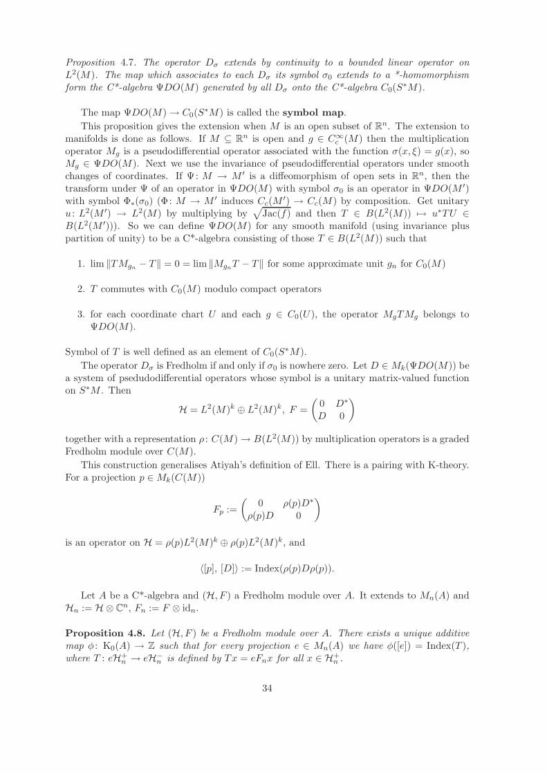
Proposition 4.7. The operator Dσ extends by continuity to a bounded linear operator onL2(M). The map which associates to each Dσ its symbol σ0 extends to a *-homomorphismform the C*-algebra ΨDO(M) generated by all Dσ onto the C*-algebra C0(S
∗M).
The map ΨDO(M) → C0(S∗M) is called the symbol map.
This proposition gives the extension when M is an open subset of Rn. The extension tomanifolds is done as follows. If M ⊆ Rn is open and g ∈ C∞
c (M) then the multiplicationoperator Mg is a pseudodifferential operator associated with the function σ(x, ξ) = g(x), soMg ∈ ΨDO(M). Next we use the invariance of pseudodifferential operators under smoothchanges of coordinates. If Ψ: M → M ′ is a diffeomorphism of open sets in Rn, then thetransform under Ψ of an operator in ΨDO(M) with symbol σ0 is an operator in ΨDO(M ′)with symbol Φ∗(σ0) (Φ: M → M ′ induces Cc(M
′) → Cc(M) by composition. Get unitaryu : L2(M ′) → L2(M) by multiplying by
√Jac(f) and then T ∈ B(L2(M)) 7→ u∗TU ∈
B(L2(M ′))). So we can define ΨDO(M) for any smooth manifold (using invariance pluspartition of unity) to be a C*-algebra consisting of those T ∈ B(L2(M)) such that
1. lim ‖TMgn − T‖ = 0 = lim ‖MgnT − T‖ for some approximate unit gn for C0(M)
2. T commutes with C0(M) modulo compact operators
3. for each coordinate chart U and each g ∈ C0(U), the operator MgTMg belongs toΨDO(M).
Symbol of T is well defined as an element of C0(S∗M).
The operator Dσ is Fredholm if and only if σ0 is nowhere zero. Let D ∈Mk(ΨDO(M)) bea system of psedudodifferential operators whose symbol is a unitary matrix-valued functionon S∗M . Then
H = L2(M)k ⊕ L2(M)k, F =
(0 D∗
D 0
)
together with a representation ρ : C(M) → B(L2(M)) by multiplication operators is a gradedFredholm module over C(M).
This construction generalises Atiyah’s definition of Ell. There is a pairing with K-theory.For a projection p ∈Mk(C(M))
Fp :=
(0 ρ(p)D∗
ρ(p)D 0
)
is an operator on H = ρ(p)L2(M)k ⊕ ρ(p)L2(M)k, and
〈[p], [D]〉 := Index(ρ(p)Dρ(p)).
Let A be a C*-algebra and (H, F ) a Fredholm module over A. It extends to Mn(A) andHn := H⊗ Cn, Fn := F ⊗ idn.
Proposition 4.8. Let (H, F ) be a Fredholm module over A. There exists a unique additivemap φ : K0(A) → Z such that for every projection e ∈ Mn(A) we have φ([e]) = Index(T ),where T : eH+
n → eH−n is defined by Tx = eFnx for all x ∈ H+
n .
34

4.2 Commutator conditions
In the definition of Fredholm module (H, F ) we have a condition [F, ρ(a)] ∈ K for all a ∈ A.In Kasparov K-homology A has to be a separable C*-algebra. For more subtle invariants,Connes allows Fredholm modules over *-algebras A, not necessarily C*-algebras. Most usefulcondition is that [F, a] ∈ Lp(H) for some p ≥ 1. There is a fine balance to be struck here:the class of algebras we allow for Fredholm modules should still have a meaningful K-theory,fairly close to the K-theory for C*-algebras. Ideally we want K-theory with the same formalproperties as K-theory for C*-algebras. Note that the K-theory for such algebras needs tobe developed from scratch. A sensible class of C*-algebras may be determined using thefollowing
Proposition 4.9 (Connes). Let A be an involutive algebra, (H, F ) an (n + 1)-summableFredholm module over A with the parity of n. Let A be the C*-algebra closure of A (in itsaction on H). Let A be the smallest involutive subalgebra of A containing A and stable underholomorphic functional calculus. Then (H, F ) is an (n+ 1)-summable Fredholm module overA.
From this one deduces that it is sufficient to restrict attention to local C*-algebras (preC*-algebras).
Proposition 4.10. Let A be a pre C*-algebra (local C*-algebra). Then
1. Any Fredholm module (H, F ) over A extends by continuity to a Fredholm module overthe associated C*-algebra A.
2. The inclusion A → A is an isomorphism on K-theory.
Proposition 4.11 (Connes). Suppose that (H, F ) is a 1-summable Fredholm module and γis an involution im[plementing the Z/2-grading on H. Then the map
τ : A→ C, a 7→ 12 Tr(γF [F, a])
is a trace on A.
Proof. DefineA := a ∈ A | [F, a] ∈ L1(H), A ⊂ A.
We have
γF [F, a] = γa− γFaF
= γa+ FaγF
= aγF 2 + FaγF − FγF + FaγF
= [F, a]γF,
where we use F 2 = 1 or the equalities are modulo K. Next
τ(ab) = 12 Tr(γF [F, ab])
= 12 Tr(γF [F, a]b + γFa[F, b])
= 12 Tr([F, a]γFb + [F, b]γFa)
= τ(ba).
35

We call τ the character of the Fredholm module (H, F ).
Theorem 4.12 (Connes). Let A be a unital C*-algebra equipped with a faithful positive traceτ , τ(1) = 1. Let (H, F ) be a Fredholm module over A such that
A := a ∈ A | [F, a] ∈ L1(H)is a dense subalgebra of A and the restriction of τ to A is the character of the Fredholmmodule (H, F ). Then A contains no nontrivial idempotents.
Proof. A is a subalgebra of A stable under holomorphic functional calculus. The inclusionA → A induces an isomorphism K0(A) → K0(A). The trace τ takes integer values (this isthe index map). If e is a projection then τ(e) = 0, 1. Because τ is faithful e = 0, 1.
Example 4.13. Let F2 be the nonabelian free group on two generators. It acts on a tree(1-dimensional simplicial complex with no loops). Let ∆0 be the set of vertices and ∆1 bethe set of edges. Denote by [x, y] for x, y ∈ ∆0 the set of vertices on the unique path from xto y, and by x0 the origin. For all x ∈ ∆0 \x0 let β(x) ∈ ∆1 be the unique edge containingx in [x, x0].
Lemma 4.14.
1. The map β : ∆0 → ∆1 is a bijection.
2. For a fixed g ∈ F2, the set of x ∈ ∆0 such that gβ(g−1x) 6= β(x) is finite and equals[x0, gx0].
Proof. 1. The inverse is given by
β−1(edge u) := vertex of u further from x0.
2. gβ(g−1x) is the edge containing x and lying in [gx0, x]. Suppose x /∈ [gx0, x].
Define a map F : l2(∆0) → l2(∆1) by
Fδx :=
δβx
for x 6= x0
0 for x = x0
Proposition 4.15.
1. F is an operator of index 1, FF∗ = 1, F∗F = 1 − px0, where px0 : l2(∆0) → Cδx0.
2. Let π0, π1 be actions of F2 on l2(∆0), l2(∆1). For all g ∈ F2 the operator π1(g)F −
Fπ0(g) is of finite rank and (l2(∆0) ⊕ l2(∆1),F) is a Fredholm module.
LetA := a ∈ C∗
r (F2) | [F , a] ∈ l2(∆0) ⊕ l2(∆1).By the proposition C[F2] ⊂ A, so A is dense in C∗
r (F2). Now from the Connes theorem oneobtains the proof of the Kadison-Kaplansky conjecture
Theorem 4.16. The algebra C∗r (F2) has no nontrivial idempotents.
Fredholm modules of this type can be constructed for any locally compact group actingon a tree (Julg, Vallette).
Theorem 4.17. Let G be any locally compact group acting on a tree such that the stabiliser ofany vertes is amenable. Then G is K-amenable.
Remark 4.18. (Christian Voigt)
36

4.3 Quantised calculus of one variable
Let f be a function on R. Find function algebras for which df := [F, f ] has a given regularity.Take H = L2(R). The Hilbert transform is given by
(Fξ)(s) = limε→0
1
πi
∫
|s−t|>ε
ξ(t)
s− tdt.
We have F 2 = 1 and [F, f ] is the operator on L2(H) associated to the kernel
k(s, t) =f(s) − f(t)
s− t
This can be transported to S1 by some conformal map. Then we obtain a Fredholm modulegiven by the data
H = L2(S1), F = 2P − 1,
where P : L2(S1) → H2(S1) is the orthogonal projection onto the Hardy space.For any f ∈ L∞(S1)
• [F, f ] is a finite rank operator if and only if f is a rational function.
• [F, f ] is compact if and only if f is of vanishing mean oscillation, that is for
Maf := sup|I|≤a
1
|I|
∫
I
|f − I(t)|dt,
where I(t) = 1|I|
∫fdx, we have lima→0Maf = 0.
• [F, f ] is in Lp(H) if and only if f is in Besov space B1pp , that is
∫ ∫|f(x+ t) − 2f(x) + f(x− t)|pt−2dxdt <∞.
4.4 Quantised differential calculus
Let (A,H, F ) be a Fredholm module over an involutive algebra A, n integer ≥ 0. We assumethat the Fredholm module is even for n even and odd for n odd. In either case it is (n+ 1)-summable: [F, a] ∈ Ln+1(H) for all a ∈ H.
For k = 0, put Ω0 = A. For k > 0
Ωk := spana0[F, a1] . . . [F, ak] | aj ∈ A.By Holder inequality, Ωk ⊂ Ln+1
k (H). Put Ω• :=⊕
k≥0 Ωk. The product in Ω• is the
operator product. We use the Leibniz rule for [F,−] to check that if ω ∈ Ωk and ω ∈ Ωk′
then ωω′ ∈ Ωk+k′
a0[F, a1] . . . [F, ak]ak+1 =k−1∑
j=1
(−1)k−ja0[F, a1] . . . [F, ajaj+1] . . . [F, ak+1]+
+(−1)ka0a1[F, a2] . . . [F, ak+1].
It is a differential graded algebra (DGA) with differential d : Ωk → Ωk+1 given by the gradedcommutator
dω = [F,ω] = Fω − (−1)|ω|ωF.
It is a graded derivation, that is
d(ω1ω2) = (dω1)ω2 + (−1)|ω1|dω2, d2 = 0.
37
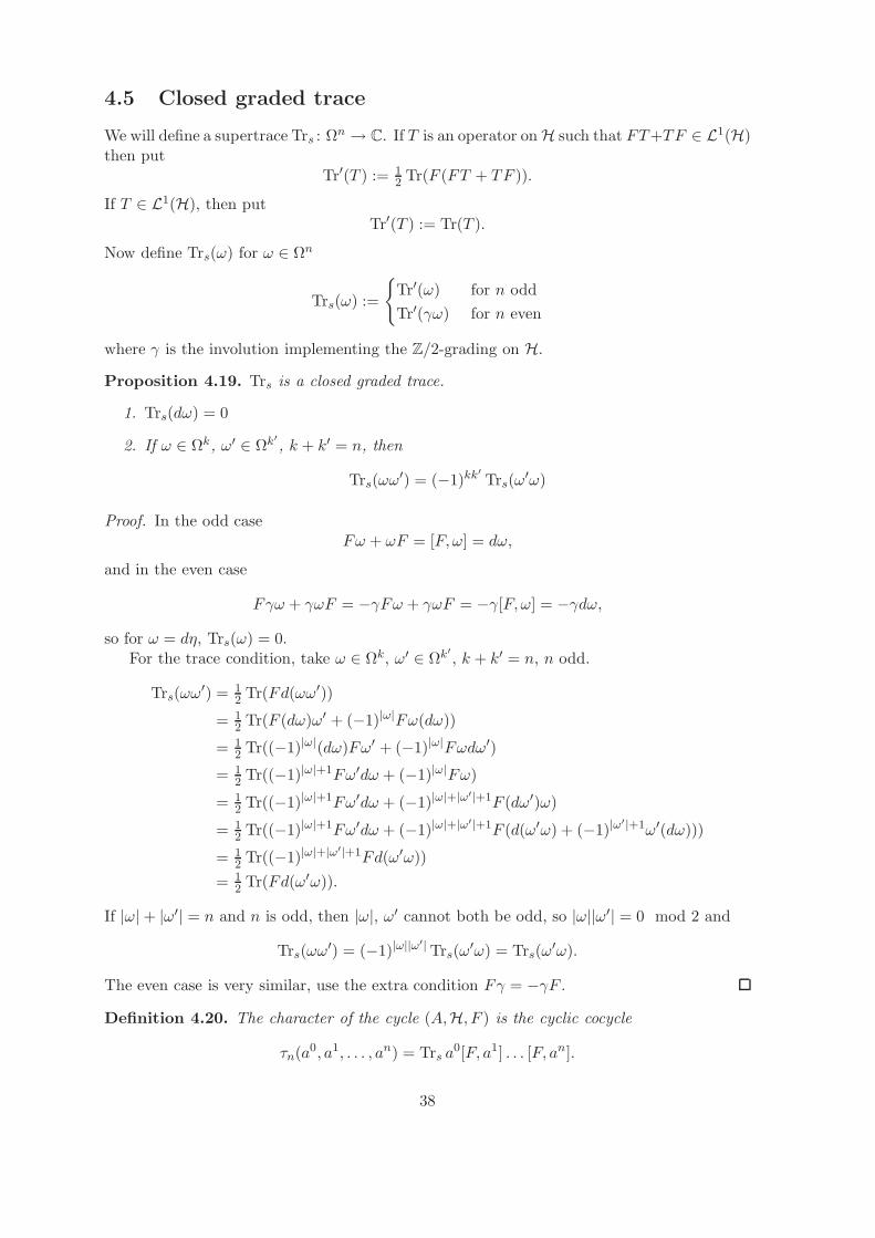
4.5 Closed graded trace
We will define a supertrace Trs : Ωn → C. If T is an operator on H such that FT+TF ∈ L1(H)then put
Tr′(T ) := 12 Tr(F (FT + TF )).
If T ∈ L1(H), then putTr′(T ) := Tr(T ).
Now define Trs(ω) for ω ∈ Ωn
Trs(ω) :=
Tr′(ω) for n odd
Tr′(γω) for n even
where γ is the involution implementing the Z/2-grading on H.
Proposition 4.19. Trs is a closed graded trace.
1. Trs(dω) = 0
2. If ω ∈ Ωk, ω′ ∈ Ωk′
, k + k′ = n, then
Trs(ωω′) = (−1)kk′
Trs(ω′ω)
Proof. In the odd caseFω + ωF = [F,ω] = dω,
and in the even case
Fγω + γωF = −γFω + γωF = −γ[F,ω] = −γdω,
so for ω = dη, Trs(ω) = 0.For the trace condition, take ω ∈ Ωk, ω′ ∈ Ωk′
, k + k′ = n, n odd.
Trs(ωω′) = 1
2 Tr(Fd(ωω′))
= 12 Tr(F (dω)ω′ + (−1)|ω|Fω(dω))
= 12 Tr((−1)|ω|(dω)Fω′ + (−1)|ω|Fωdω′)
= 12 Tr((−1)|ω|+1Fω′dω + (−1)|ω|Fω)
= 12 Tr((−1)|ω|+1Fω′dω + (−1)|ω|+|ω′|+1F (dω′)ω)
= 12 Tr((−1)|ω|+1Fω′dω + (−1)|ω|+|ω′|+1F (d(ω′ω) + (−1)|ω
′|+1ω′(dω)))
= 12 Tr((−1)|ω|+|ω′|+1Fd(ω′ω))
= 12 Tr(Fd(ω′ω)).
If |ω| + |ω′| = n and n is odd, then |ω|, ω′ cannot both be odd, so |ω||ω′| = 0 mod 2 and
Trs(ωω′) = (−1)|ω||ω
′| Trs(ω′ω) = Trs(ω
′ω).
The even case is very similar, use the extra condition Fγ = −γF .
Definition 4.20. The character of the cycle (A,H, F ) is the cyclic cocycle
τn(a0, a1, . . . , an) = Trs a0[F, a1] . . . [F, an].
38

Difficult problem: provide an explicit formula for this cocycle in terms of data defining theFredholm module. The cyclic cocycle seems to depend on n, but in fact there is no problemhere.
Recall Connes’ periodicity operator S : HCn(A) → HCn+2(A),
. . .HHn−1(A,A) → HCn(A) → HCn+2(A) → HHn+2(A,A) → HCn+1(A) → . . .
Proposition 4.21. The characters τn+2q satisfy
τm+2 = − 2
m+ 2Sτm, m = n+ 2q,
so the cocycles together determine a class in periodic cyclic cohomology
HP•(A) = lim−→
(HCn(A), S)
Definition 4.22. Let (A,H, F ) be a finitely summable Fredholm module over an involutivealgebra A. The Chern character ch•(H, F ) ∈ HP•(A) is the periodic cyclic cohomologyclass whose components are the following cyclic cocycles for large enough n:
(−1)n(n−1)
2 Γ(n
2+ 1
)Tr′(γa0[F, a1] . . . [F, an])
for n even (even Fredholm module), and
√2i(−1)
n(n−1)2 Γ
(n2
+ 1)
Tr′(γa0[F, a1] . . . [F, an])
for n odd.
Remark 4.23. Let ΩA be the universal differential graded algebra, N-graded. It is also Z/2-graded algebra with respect to the Fedosov product
ω1 ω2 = ω1ω2 + (−1)|ω1|dω1dω2.
Supertraces Tr : ΩA→ C are linear maps which satisfy the suspension conditions.
Theorem 4.24 (Connes, Cuntz-Quillen). There is one-to-one correspondence between (har-monic) periodic cocycles and supertraces on ΩA.
(ΩA, b,B) → (entire) cyclic type homology theories.
4.6 Index pairing formula
From Atiyah and Kasparov we have the following result:
Proposition 4.25. Let A be an involutive algebra, (H, F ) a Fredholm module over A. Forq ∈ N let (Hq, Fq) be the Fredholm module over Mq(A) = A ⊗ Mq(C), Hq = H ⊗ Cq,
Fq = F ⊗ idq. Extend the action of A on H to a unital action of A.
1. In the even case: let γ be the involution for Z/2-grading and e ∈Mq(A) be a projection.Then the operator
π−q (e)Fqπ+q (e) : π+
q (e)H+q → π−q (e)H−
q
is Fredholm. There is an additive map
ϕ : K0(A) → Z
given byϕ([e]) := Index(π−q (e)Fqπ
+q (e)).
39

2. In the odd case: let u ∈ GLq(A), E = 1+F2 . Then
Eqπq(u)Eq : EqHq → EqHq
is Fredholm. There is an additive map
ϕ([u]) := Index(Eqπq(u)Eq).
When A is a C*-algebra, K1(A) in 2. is the topological K-theory Ktop1 (A) as defined
before.In both cases, the index map depends only on the class
[(H, F )] ∈ KKi(A,C) = Ki(A),
the K-homology of A. This can be regarded as a pairing
Ki(A) × Ki(A) → Z.
Proposition 4.26. For x ∈ Ki(A)
ϕ(x) = 〈x, ch∗(H, F )〉 = 〈ch(x), ch(H, F )〉.
On the right hand side in the proposition we have a pairing between K-theory and cyclicsohomology. A more symmetric formula would use a complementary Chern character on K-homology. Since Connes’ construction, formulae were given for Chern characters in K-theorywith values in HP•(A).
The pairing has simple definition. Let τ ∈ HCn(A). Take τ ⊗ Tr: Mk(A) → C for everyk,
τ ⊗ Tr(a0 ⊗ T 0, a1 ⊗ T 1, . . . , an ⊗ T n) = τ(a0, . . . , an)Tr(T 0, . . . .Tn).
Then
〈[e], [τ ]〉 =1
m!(τ ⊗ Tr)(e, e, . . . , e).
All this is explained in Quillen’s higher traces paper.
4.7 Kasparov’s K-homology
Let (ρ,H, F ) be a Fredholm module, U : H′ → H be a unitary isomorphism (preservingthe grading if there is one). Then (U∗ρU,H′, U∗FU) is also a Fredholm module unitarilyequivalent to (ρ,H, F ).
Definition 4.27. Suppose (ρ,H, Ft) is a family of Fredholm modules parametrized by t ∈[0, 1], H is fixed Hilbert space, and Ft varies with t. If the function t 7→ Ft is norm continuous,then we say that the family defines an operator homotopy between the Fredholm modules(ρ,H, F0) and (ρ,H, F1) an that these two Fredholm modules are Operator homotopic.
Definition 4.28. If (ρ,H, F ) and (ρ,H, F ′) are Fredholm modules on H and (F − F ′)ρ(a)is compact for all a ∈ A, then we call F a compact perturbation of F ′.
Compact perturbation impliest operator homotopy - the linear path from F to F ′ definesan operator homotopy.
One can perform a compact perturbation to make F exactly self adjoint, F 7→ 12(F +F ∗).
40

Definition 4.29. K-homology of a C*-algebra A, Kp(A), is an abelian group with onegenerator [x] for each unitary equivalence class of graded Fredholm modules over A with thefollowing relations:
1. If x0 and x1 are operator homotopic graded Fredholm modules, then [x0] = [x1] ∈ Kp(A).
2. If x0 and x1 are graded Fredholm modules then [x0 ⊕ x1] = [x0] + [x1] in Kp(A), wherex0 ⊕ x1 = (A,H0 ⊕H1, ρ0 ⊕ ρ1, F0 ⊕ F1).
We have p = 0 for graded, and p = 1 for ungraded Fredholm modules.
Remark 4.30. p-graded Fredholm modules give rise to lower K-homology K−p(A) for all p ∈ N.
Kp(A) is a contravariant functor in A. If α : A′ → A is a *-homomorphism, and (ρ,H, F )is a Fredholm A-module, then (ρ α,H, F ) is a Fredholm A′-module. We have an inducedmap
α∗ : Kp(A) → Kp(A′).
Definition 4.31. A Fredholm module (ρ,H, F ) is degenerate if and only if
[ρ(a), F ] = 0
ρ(a)(F 2 − 1) = 0
ρ(a)(F − F ∗) = 0
for all a ∈ A.
Proposition 4.32. The class of a degenerate Fredholm module is zero in Kp(A).
Proof. Let x = (ρ,H, F ) be a degenerate Fredholm module. Then
x′ := (ρ′,H′, F ′), H′ :=
∞⊕
i=1
, F ′ :=
∞⊕
i=0
F, ρ′ :=
∞⊕
i=0
ρ.
This is a Fredholm module, since x is degenerate. But x⊕ x′ is unitarily equivalent to x′, so[x⊕ x′] = [x] + [x′] = [x′] and [x] = 0.
Lemma 4.33. For a graded Fredholm module (ρ,H, F ) denote by (ρop,Hop,−F op) the Fred-holm module with the opposite grading. This is the additive inverse to (ρ,H, F ).
Proof. Let
Ft :=
(cos(π
2 t)F sin(π2 t)Id
sin(π2 t)Id − cos(π
2 t)F
),
F0 =
(F 00 −F
), F1 =
(0 11 0
).
This is the operator homotopy on H ⊕Hop from F0 = F ⊕ (−F op) to the degenerate F1 =(0 11 0
).
Example 4.34. K0(C) = Z. If (ρ,H, F ) is a Fredholm module over C, then ρ(1) =: p is aprojection in B(H) and up to compact perturbation (ρ,H, F ) is the direct sum of (ρ, pH, pFp)and (ρ, (1− p)H, (1− p)F (1− p)). The second module carries the zero action of C. The firstis determined by pFp. Put
(ρ,H, F ) 7→ Index(pFp).
This gives a homomorphism K0(C) → Z. Since an essentially unitary operator with indexzero is a compact perturbation of a unitary, this map is an isomorphism.
41

Lemma 4.35. Let (ρ,H, F ) be a Z/2Z-graded Fredholm module. Assume that there exists aself adjoint odd-graded involution E : H → H which commutes with ρ (the action of A) andanticommutes with F . Then the Fredholm module (ρ,H, F ) represents the zero element inK0(A).
Proof. Let Ft := cos(t)F + sin(t)E. This is an operator homotopy from F to the degenerateoperator E.
In particular putting tho ungraded Fredholm modules together produces a degenerateFredholm module. Conversely, if we ignore Z/2Z-grading on an even Fredholm module thenthe resulting odd Fredholm module represents the zero element. A possible argument is asfollows. A Z/2Z-graded module is given by the data H = H+ ⊕H−,
F =
(0 u∗
u 0
), ρ =
(ρ(a) 0
0 ρ(a)
).
We construct an operator homotopy
Ft =
(cos(π
2 t)Id sin(π2 t)v
sin(π2 t)u cos(π
2 t)Id
)
F0 =
(1 00 1
), F1 =
(0 vu 0
).
For this we need to assume that F1 is an involution.
42

Chapter 5
Boundary maps in K-homology
5.1 Relative K-homology
Definition 5.1. Let J be an ideal in A. A relative Fredholm module for (A,A/J) is atriple (ρ,H, F ), where
1. H is a separable Hilbert space
2. ρ : A→ B(H) is a *-representation
3. for all a ∈ A, j ∈ J
(F 2 − 1)ρ(j) ∼ 0
(F − F ∗)ρ(j) ∼ 0
[F, ρ(a)] ∼ 0
One defines also the graded version.The relative Fredholm modules generate relative K-homology Kp(A,A/J). The natural
mapKp(A,A/J) → Kp(J)
is an isomorphism (excision).To any extension of separable C*-algebras one can associate an exact sequence of lenght
six
K1(A/J) // K1(A) // K1(J)
K0(J)
OO
K0(A)oo K0(A/J)oo
We can give an explicit description of the boundary maps in this six term exact sequence.
5.2 Semisplit extensions
There is ono-to-one correspondence between extensions of A by K(H) and unitary equivalenceclasses of *-homomorphisms φ : A→ Q(H)
0 // K(H) // E //
A //
φ
0
0 // K(H) // B(H)π // Q(H) // 0
43

Definition 5.2. A unital injective extension φ : A → Q(H) is semisplit if there is anotherunital extension φ′ : A→ Q(H) such that φ⊕ φ′ is split extension.
Definition 5.3. Let the extension
0 → J → A→ A/J → 0
be semisplit by a completely positive map A/J → A. Let ρ : A → B(H) be a representationof A on a separable Hilbert space H. A Stinespring dilation associates to the above datais a *-homomorphism
ψ =
(ψ11 ψ12
ψ21 ψ22
): A/J → B(H⊕H′),
where H′ is a separable Hilbert space and ψ11(x) = ρ(s(x)).
The existence of such extension follows from Stinespring’s theorem.
Theorem 5.4 (Stinespring). A unital linear map σ : A→ B(H) is absolutely positive if andonly if there are
1. an isometry v : H → H
2. a nondegenerate representation ρ : A→ B(H) such that σ(a) = v∗ρ(a)v
In Z/2Z-graded case one applies this to each component separately.
Proposition 5.5. Take an extension as above. Let (ρ,H, F ) be a selfadjoint relative Fredholmmodule (graded or ungraded). Let ψ : A/J → B(H⊕H′) be a Stinespring dilaton. Then theboundary maps are given by
1. ∂ : K0(A,A/J) → K1(A/J) : the cycle (ρ,H, F ) is graded Fredholm module. Assumethat F 2 is a projection (this can always be done). Let Q± be the components of theprojection 1 − F 2 on H±. Then the projections
(Q± 00 0
)∈ B(H⊕H′)
commute modulo compacts with ψ(x) for all x ∈ A/J and so define ungraded Fredholmmodules. Their difference represents a class of ∂[ρ,H, F ] (if ρ : A→ B(H), P ∈ B(H)is a projection such that [P, ρ(a)] ∈ K for all a ∈ A, then (ρ,H, F = 2P − 1) is anungraded Fredholm module over A).
2. ∂ : K1(A,A/J) → K0(A/J): the cycle (ρ,H, F ) is ungraded Fredholm module. Then
(eiπF 0
0 −1
)∈ B(H⊕H′)
is unitary on H⊕H′ commuting with ψ. The corresponding Fredholm module representsa class of ∂[ρ,H, F ].
44

5.3 Schrodinger pairs
Recall that we call an operator X ∈ B(H) contractive if and only if ‖X‖ ≤ 1. For aselfadjoint contractive operator X we define Xb to be a commutative C*-subalgebra of B(H)consisting of all ψ(X) for ψ ∈ C0(−1, 1).
Definition 5.6. Let X,Y be contractive operators on H. The pair (X,Y ) is a Schrodinger
pair if and only if
1. Y commutes with Xb modulo K(H).
2. Xb · Y b ⊆ K(H).
We call (X,Y ) a graded Schrodinger pair if the commutator in 1 is graded.
We call (X,Y ) a strong Schrodinger pair if Y commutes with X.
Example 5.7. Let H = L2(R), X multiplies by x 7→ x√1+x2
, and Y multiplies the Fourier
transform by ξ 7→ ξ√1+ξ2
(Xf)(x) :=x√
1 + x2f(x)
(Y f)(ξ) :=ξ√
1 + ξ2f(ξ)
These are the position and momentum operators in quantum mechanics and (X,Y ) is astrong Schrodinger pair.
Example 5.8. Let (ρ,H, F ) be an ungraded Fredholm module over J , where J is an ideal insome C*-algebra A and ρ extends to A. If a is an element of A such that a2 − 1 ∈ J , thenX = ρ(a), Y = F constitute Schrodinger pair.
If the extension of ρ makes (ρ,H, F ) into a relative Fredholm module (i.e. [F, ρ(a)] ∼ 0for all a ∈ A) then (X,Y ) is a strong Schrodinger pair.
Example 5.9. Let H = L2([−1, 1]). Define operators
(Tψ)(x) = ψ(−x),(Sψ)(x) = xψ(x).
If f ∈ C0(−1, 1) then f(T ) = 0 and (T, S) is a Schrodinger pair. If f is an odd function on[−1, 1] such that f(−1) = f(1) = 0, then
[f(S), T ] = −2f(S)T
which is not compact. Thus (S, T ) is not a Schrodinger pair.
Definition 5.10. Let (X,Y ) be a Schrodinger pair. The Schrodinger operator is givenby
V (X,Y ) := εX + (1 −X2)12Y,
where ε = i in the ungraded, and ε = 1 in the graded case.
Proposition 5.11. Let (X,Y ) be a (graded) strong Schrodinger pair. Then
45

1. in the ungraded case the Schrodinger operator
V (X,Y ) = iX + (1 −X2)12Y
is essentially unitary and so Fredholm,
2. in the graded case the Schrodinger operator
V (X,Y ) = X + (1 −X2)12Y
is essentially selfadjoint graded and Fredholm.
Proposition 5.12.
1. In the ungraded case
IndexV (X,Y ) = IndexV (Y,X).
2. In the graded case
IndexV (X,Y ) = − IndexV (Y,X).
Proposition 5.13. If X,Y commute modulo compacts with a representation of C*-algebraB then
1. in the graded case
[V (X,Y )] = [V (Y,X)] ∈ K0(B),
2. in the ungraded case
[V (X,Y )] = −[V (Y,X)] ∈ K1(B).
Proof.
V (X,Y )2 − 1 ∼ X2 + (1 −X2)Y 2 − 1
= −(1 −X2)(1 − Y 2) ∈ K(H),
because XY + Y X ∼ 0. Next
V (X,Y )V (Y,X) + V (Y,X)V (X,Y ) ∼ 2(Y (1 −X2)12Y +X(1 − Y 2)
12X) ≥ 0,
so Fredholm modules associated with V (X,Y ) and V (Y,X) are homotopic, which is a con-sequence of the following
Proposition 5.14. If (ρ,H, F0) and (ρ,H, F1) are (graded) Fredholm modules such thatρ(a)(F0F1 + F1F0)ρ(a
∗) are positive modulo compacts for all a ∈ A, then F0 and F1 areoperator homotopic.
Recall the index map on K-homology
Index: Kp(A) → Z, (ρ,H, F ) 7→ inf F.
If F =
(0 vu 0
), then IndexF = Indexu.
46

Lemma 5.15. Let (X,Y ) be a Schrodinger pair on an ungraded Hilbert space H. Put PY :=12(1 + Y ). Then the operator
W1(X,Y ) := eiπXPY − (1 − PY )
is essentially unitary and Fredholm. Furthermore
IndexW1(X,Y ) = IndexV (X,Y ).
Proof. Denote for convinience S := sin(π2X). From the definition of Schrodinger pair we
know that
• Y commutes with Sb modulo compacts,
• (1 − S2)(1 − Y 2) is compact.
Write
e−i π2XW1(X,Y ) = ei
π2XPY − e−i π
2X(1 − PY )
= (cos(π
2X) + i sin(
π
2X))PY − (cos(
π
2X) − i sin(
π
2X))(1 − PY )
= ((1 − S2)12 + iS)PY − ((1 − S2)
12 − iS)(1 − PY )
= ((1 − S2)12 + iS)(1
2 (1 + Y )) − ((1 − S2)12 − iS)(1
2 (1 − Y ))
= iS + (1 − S2)12Y
= V (S, Y ).
Thus the operator W1(X,Y ) is essentially unitary and homotopic to V (S, Y ) through thepath
t 7→ e−itπ2XW1(X,Y ), t ∈ [0, 1],
so [W1(X,Y )] = [V (S, Y )]. But S is homotopic to X via a path Xt := tX + (1 − t)S, and(Xt, Y ) are a Schrodinger pairs for all t. This gives a homotopy V (Xt, Y ) and [V (X,Y )] =[V (S, Y )] = W1(X,Y ).
Lemma 5.16. Let (X,Y ) be a graded Schrodinger pair on a graded Hilbert space H. Supposealso that
1. QX = 1 −X2 is a projection
2. there exists a self adjoint involution Y0 on H which commutes with QX modulo thecompacts.
Then the operator W2(X,Y ) = Y QX+Y0(1−QX) is essentially self-adjoint, graded, Fredholm,and
IndexW2(X,Y ) = IndexV (X,Y ).
Proof. Let
Xt := cos(π
2t)X + sin
(π2t)Y0(1 −QX).
47

Then for all t ∈ [0, 1] we have
Xt(Y QX) ∼ 0
(Y QX)Xt ∼ 0
X2t ∼ 1 −QX
Indeed:
X2t = cos2
(π2t)X2 + sin2
(π2t)Y0(1 −QX)Y0(1 −QX)
+ cos(π
2t)
sin(π
2t)XY0(1 −QX) + sin
(π2t)
cos(π
2t)Y0(1 −QX)X
= cos2(π
2t)X2 + sin2
(π2t)
(1 −QX)2.
The operator QX is a projection onto kerX. The path t 7→ Y QX + Xt gives an operatorhomotopy from V (X,Y ) to W2(X,Y ). Indeed:
QXXt = cos(π
2t)QXX︸ ︷︷ ︸
0
+ sin(π
2t)QXY0(1 −QX) ∈ K(H).
Recall that V (X,Y ) = X + (1 −X2)12Y . Thus for
t = 0 : Y QX +Xt = Y Qx +X ∼ V (X,Y ),
t = 1 : Y QX + Y0(1 −QX) = W2(X,Y ).
5.4 The index pairing
Proposition 5.17 (odd case). Let A be a unital C*-algebra and suppose given
1. an ungraded unital Fredholm module (ρ,H, F ) over A,
2. a unitary u in a matrix algebra Mk(A) over A.
Let Pk = 1⊗ 12(1+F ) : Hk → Hk and U = (1⊗ρ)(u) : Hk → Hk be a unitary operator. Then:
1. the operator W := PkUPk − (1 − Pk) : Hk → Hk is essentially unitary, so Fredholm.
2. The Fredholm index of W = PkUPk − (1 − Pk) depends only on [U ] ∈ K1(A) and[P ] ∈ K1(A). This index gives a pairing
K1(A) × K1(A) → Z
([u], [F ]) 7→ Index(PkUPk − (1 − Pk)).
Assume that F 2 = 1 so that Pk is a projection. Then Hk = imPk ⊕ im(1 − Pk) andW = PkUPk ⊕ (−Id) with respect to this decomposition. The second summand has indexzero, and this is precisely the pairing that was defined before.
By definition of Fredholm module Pk and U commute modulo compacts K(Hk) and
W ∗W ∼ PkU∗UPk + (1 − Pk) ∼ 1.
Thus W ∗W ∼ 1 and similarly WW ∗ ∼ 1. The map ([u], [F ]) 7→ IndexW is additive andstable under compact perturbations and homotopies.
48
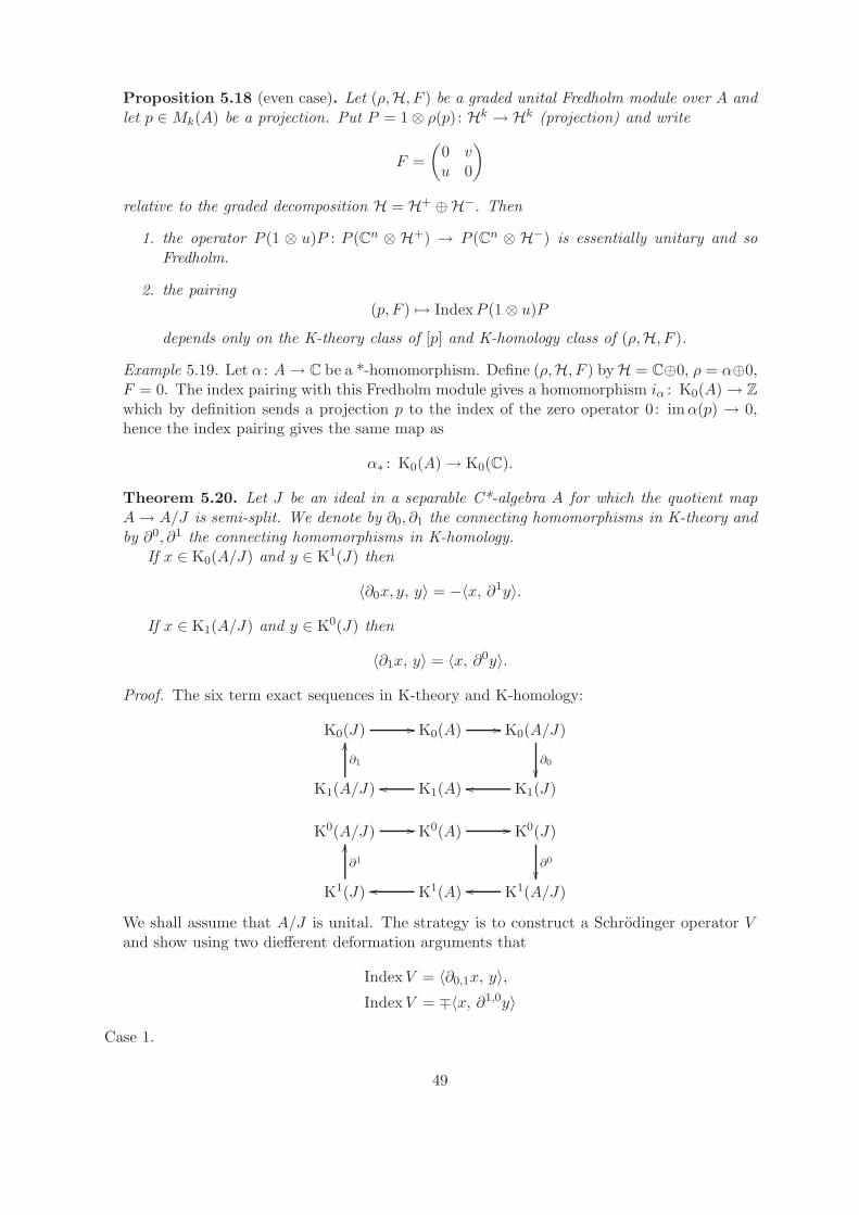
Proposition 5.18 (even case). Let (ρ,H, F ) be a graded unital Fredholm module over A andlet p ∈Mk(A) be a projection. Put P = 1 ⊗ ρ(p) : Hk → Hk (projection) and write
F =
(0 vu 0
)
relative to the graded decomposition H = H+ ⊕H−. Then
1. the operator P (1 ⊗ u)P : P (Cn ⊗ H+) → P (Cn ⊗ H−) is essentially unitary and soFredholm.
2. the pairing(p, F ) 7→ IndexP (1 ⊗ u)P
depends only on the K-theory class of [p] and K-homology class of (ρ,H, F ).
Example 5.19. Let α : A→ C be a *-homomorphism. Define (ρ,H, F ) by H = C⊕0, ρ = α⊕0,F = 0. The index pairing with this Fredholm module gives a homomorphism iα : K0(A) → Z
which by definition sends a projection p to the index of the zero operator 0: imα(p) → 0,hence the index pairing gives the same map as
α∗ : K0(A) → K0(C).
Theorem 5.20. Let J be an ideal in a separable C*-algebra A for which the quotient mapA→ A/J is semi-split. We denote by ∂0, ∂1 the connecting homomorphisms in K-theory andby ∂0, ∂1 the connecting homomorphisms in K-homology.
If x ∈ K0(A/J) and y ∈ K1(J) then
〈∂0x, y, y〉 = −〈x, ∂1y〉.
If x ∈ K1(A/J) and y ∈ K0(J) then
〈∂1x, y〉 = 〈x, ∂0y〉.
Proof. The six term exact sequences in K-theory and K-homology:
K0(J) // K0(A) // K0(A/J)
∂0
K1(A/J)
∂1
OO
K1(A)oo K1(J)oo
K0(A/J) // K0(A) // K0(J)
∂0
K1(J)
∂1
OO
K1(A)oo K1(A/J)oo
We shall assume that A/J is unital. The strategy is to construct a Schrodinger operator Vand show using two diefferent deformation arguments that
IndexV = 〈∂0,1x, y〉,IndexV = ∓〈x, ∂1,0y〉
Case 1.
49

Step 1. Suppose we are given a short exact sequence of separable C*-algebras
0 → J → A→ A/J → 0.
Let (ρ,H, F ) be an ungraded Fredholm module for J . Let p ∈ Mk(A/J) be aprojection and let a ∈Mn(A) be a lift of p. Then
X = (1 ⊗ ρ)(2a− 1), Y = 1 ⊗ F
form a Schrodinger pair. If (ρ,H, F ) is a relative Fredholm module for (A,A/J)then (X,Y ) is a strong Schrodinger pair. The map
(p, F ) 7→ IndexV (X,Y )
defines pairingsK0(A/J) ⊗ K1(J) → Z
K0(A/J) ⊗ K1(A,A/J) → Z
which are compatible with the excision isomorphism K1(A,A/J)≃−→ K1(J). For
x ∈ K0(A/J), y ∈ K1(J) denote this pairing by x · y.Step 2. x · y = −〈x, ∂1y〉.
Assume that x = [p] with p ∈ A/J (similar arguments works for matrices) andy = [(ρ,H, F )].
∂1y =
[(ψ,H⊕H′,
(eiπF 0
0 −1
))],
where ψ : A/J → B(H⊕H′) is a representation obtained from a completely positive
section s : A/J → A by composing with ρ and then applying Stinespring’s dilation.
Put
X = ψ(2p − 1) ∈ B(H⊕H′), X =
(X11 X12
X21 X22
).
Then X11 = ρ(2a − 1), a ∈ A is a lift of p ∈ A/J . This is the operator whichappears in the definition of Schrodinger pairing.
If Y = F then X = X11 and Y form a strong Schrodinger pair and x · y =IndexV (X,Y ). Now
Y =
(Y 00 1
), X =
(X11 X12
X21 X22
)
form a Schrodinger pair (not strong). Now
(X)2 = ψ((2p − 1)2) = 1
X12X21 = 1 −X211 = 1 −X2 ∈ ρ(J).
Furthermore X = ρ(2a − 1), and 2a − 1 lifts 2p − 1, (2p − 1)2 = 1, so (2a −1)2 = 1 + j, where j ∈ J . Now X2 = ρ((2a − 1)2) = 1 + ρ(j) and we get therequired compactness conditions from the definition of Fredholm module. Indeed,1 − Y 2 = 1 − F 2, so
(1 − F 2)ρ(j) = (1 − F 2)(1 −X2) ∈ K(H).
50

Essentially the same calculation will show that
V (Y , X) ∼(V (X,Y ) 0
0 1
).
By the proposition
IndexV (Y , X) = IndexV (Y,X) = − IndexV (X,Y ) = −x · y.
If P bX= 1
2(X + 1) = ψ(p) then using the formula for ∂1y
〈x, ∂1y〉 = Index
((eiπF 0
0 −1
)P bX
− (1 − P bX)
)
= Index(eiπFP bX− (1 − P bX
))
= IndexW1(Y , X).
But we have seen that Index(W1(Y , X)) = Index(V (Y , X)) so
〈x, ∂1y〉 = IndexW1(Y , X) = Index(V (Y , X)) = Index(V (X,Y )) = −x · y.
Step 3. As before, assume that a projection p ∈ A/J has a lift to a self adjoint a ∈ A, andthat y is represented by (ρ,H, F ). Put X := ρ(2a − 1), Y := F . The boundarymap in K-theory gives
∂0x = [e2πia] ∈Mk(J).
The index pairing is
〈∂0x, y〉 = Index((1 ⊗ ρ)e2πiaPY + (1 − PY )),
where PY = 12(1 + Y ). Put T := −e−iπXPY + (1 − PY ) = −W1(X,Y ). Then
〈∂0x, y〉 = Index(T ) = Index(W1(X,Y )) = Index(V (X,Y )) = x · y,
so〈∂0x, y〉 = −〈x, ∂1y〉.
Case 2.
Step 1. In the graded case take a short exact sequence
0 → J → A→ A/J → 0
and a graded Fredholm module (ρ,H, F ) for (A,A/J). Let u ∈ Mn(A/J) be aunitary matrix and a ∈Mn(A) a lift of u to A. Then
X =
(0 (1 ⊗ ρ)(a∗)
(1 ⊗ ρ)(a) 0
), Y =
(1 ⊗ F 0
0 −1 ⊗ F
)
on a graded Hilbert space Cn ⊗ H ⊕ Cn ⊗ Hop form a strong Schrodinger pair.Furthermore
(u, F ) 7→ Index(V (X,Y ))
defines a bilinear pairing K1(A/J) × K0(A,A/J) → Z denoted again by x · y.
51

Step 2. For x ∈ K1(A/J), y ∈ K0(A,A/J) we have x · y = 〈x, ∂0y〉. Assume thaty = [(ρ,H, F )] is a graded relative module for K0(A,A/J). Use the descritptionof boundary map ∂0 : K0(J) → K1(A/J), so assume that (ρ,H, F ) is paritallyisometric i.e. Q := 1 − F 2 is a projection with graded components Q±. Then∂0[y] = [Q+] − [Q−].
Assume that u is a unitary in A/J representing x. Define
X :=
(0 ρ(a∗)
ρ(a) 0
), Y :=
(F 00 −F
)
on H⊕Hop. Then by definition x · y = Index(V (X,Y )) = Index(V (Y,X)). Put
QY := 1 − Y2 =
(Q 00 Q
).
The operator X0 =
(0 11 0
)is odd and commutes modulo compacts with Y 2. By
lemma (??) for W2(Y,X) := XQY +X0(1 −QY )
Index(V (Y,X)) = Index(W2(Y,X)) = 〈x, [Q+]〉 − 〈x, [Q−]〉 = 〈x, ∂0y〉.
Step 3. Assume that A is unital. Let y ∈ K0(A,A/J) be represented by a graded relativeFredholm module (ρ,H, F ), and x ∈ K1(A/J) represented by a unitary u ∈ A/J .Then u lifts to a partial isometry a ∈ A. Put
X :=
(0 ρ(a∗)
ρ(a) 0
), Y :=
(F 00 −F
).
Then x · y = Index(V (X,Y )), and
QX := 1 −X2 =
(ρ(1 − a∗a) 0
0 ρ(1 − aa∗)
)
is a projection onto kerX. We have furthermore
V (X,Y ) = X + (1 −X2)Y = (1 −QX)X(1 −QX) +QXY QX ,
Index(V (X,Y )) = Index(QXY QX).
Using the boundary formula for the boundary map in K-theory
∂1x = [1 − a∗a] − [1 − aa∗] ∈ K0(J)
we get
Index(QXY QX) = 〈∂1x, y〉.
52

5.5 Product of Fredholm operators
The construction of the index pairing by means of Schrodinger operators is a special case ofthe Kasparov product.
Let F1, F2 be graded Fredholm operators, Fi =
(0 U∗
i
Ui 0
), on a graded Hilbert spaces H1,
H2. A graded Fredholm operator F on H1⊗H2 (graded Hilbert space product) is aligned
with Fi if F (Fi⊗1) + (Fi⊗1)F ≥ 0 modulo compacts.
Proposition 5.21. Let Fi be graded Fredholm operator on Hi, i = 1, 2. There exist gradedFredholm operators on H1⊗H2 which are simultaneously aligned with F1 and F2. Any twosuch operators have the same index.
Proof. Define F ∈ B(H1) ⊗B(H2) by F := F1⊗1 + 1⊗F2. Then
F (Fi⊗1) + (Fi⊗1)F = 2(F 2i ⊗ 1) ≥ 0,
so F is aligned with both F1, F2. Moreover
Index(F ) = Index(F1) · Index(F2),
so F is a good model for the product of Fi, but we need F 2 − 1 ∼ 0.
Lemma 5.22. Let Fi are graded Fredholm operators on Hi, and Ni a positive operators onH1⊗H2 such that
1. N21 +N2
2 = 1,
2. [Ni, Fj⊗1] ∼ 0, i, j = 1, 2,
3. Ni(Fi⊗1)2 ∼ Ni.
Then
F := N121 (F1⊗1)N
121 +N
122 (1⊗f2)N
122
is an odd Fredholm operator aligned with F1, F2. Moreover F 2 ∼ 1.
Let (ρi,Hi, Fi) be graded Fredholm modules over C*-algebras Ai, i = 1, 2. Define arepresentation of A1 ⊗A2 on B(H), H = H1⊗H2:
ρ : A1 ⊗A2 → B(H1 ⊗H2), ρ(a1 ⊗ a2) := ρ1(a1)ρ2(a2).
We say that Fredholm module (ρ,H, F ) is aligned with (ρi,Hi, Fi) if
ρ(a)(F (Fi⊗1) + (Fi⊗1)F )ρ(a∗) ≥ 0 mod K(H)
for all a ∈ A1 ⊗A2, and if ρ(a)F derives K(H1) ⊗B(H2) for all a ∈ A1 ⊗A2, that is
[ρ(a)F,K1 ⊗ T2] ∈ K1(H1) ⊗B(H2), ∀K1 ⊗ T2 ∈ K(H1) ⊗B(H2).
Proposition 5.23. Let (ρi,Hi, Fi) be graded Fredholm modules over separable C*-algebrasA1 and A2. There exist Fredholm modules F which are aligned with F1 and F2. Moreoverthe operator homotopy class of such an F is determined uniquely by the operator homotopyclasses of F1 and F2.
The hard part is to prove existence of such Fredholm modules.
Definition 5.24. The module F from the proposition is the product of F1 and F2.
53

Chapter 6
Equivariant K-homology of spaces
Assume X is a Hausdorff space on which a discrete group Γ acts by homeomorphisms.
Definition 6.1. The action of Γ is proper if and only if for every x, y ∈ X there existneighbourhoods Ux, Uy such that the set
γ ∈ Γ | γUx ∩ Uy 6= ∅
is finite.
If Γ is discrete, this definition is equivalent to the following one:
Definition 6.2. The action of Γ is proper if and only if the quotient X/Γ is Hausdorff andfor every x ∈ X there exists (U,H, ρ) such that U is a Γ-invariant neighbourhood of x, H isa finite subgroup of Γ, and ρ : U → Γ/H is a Γ-equivariant map.
Another definition is:
Definition 6.3. The action X × Γ → X is proper if and only if the map
X × Γ → X ×X, (x, γ) 7→ (x, xγ)
is proper (preimage of a compact set is compact).
Examples 6.4.
1. If p : X → Y is a locally trivial covering space with group Γ, then the Γ-action on X isproper.
2. Any action by a finite group is proper.
3. If Γ acts simplicially on a simplicial complex X, then the action is proper if and only ifthe vertex stabilizers are finite.
Let X be a locally compact space equipped with a proper action by a discrete group Γ.
Definition 6.5. A generalized elliptic Γ-equivariant operator on X is a triple (U, π, F )such that
• U is a unitary representation of Γ on some Hilbert space H,
54

• π is a *-representation of C0(X) by bounded operators on H which is covariant, that is
π(f γ−1) = Uγπ(f)Uγ
for all f ∈ C0(X),
• F is bounded self adjoint operator which is Γ-equivariant, that is UγF = FUγ, and
π(f)(F 2 − 1), [π(f), F ]
are compact for all f ∈ C0(X).
Definition 6.6. Two cycles α0 = (U0, π0, F0), α1 = (U1, π1, F1) are operator homotopic,α0 ∼h α1, if and only if U0 = U1, π0 = π1 and there exists a path t 7→ Ft, t ∈ [0, 1] such thatαt = (U0, π0, Ft) is a Γ-elliptic operator.
We say that α0, α1 are equivalent, α0 ∼ α1, if and only if there exist degenerate operatorsβ0, β1 such that α0 ⊕ β0 ∼h α1 ⊕ β1, up to unitary equivalence.
Definition 6.7. The equivariant K-homology groups of X are defined by
• KΓ0 (X) = equivalence classes of Z/2Z-graded Γ-elliptic operators, that is
Uγ =
(U+
γ 0
0 U−γ
), π =
(π+ 00 π−
), F =
(0 p∗
p 0
),
• KΓ1 (X) = equivalence classes of Γ-elliptic operators.
Remark 6.8. Kasparov uses a weaker form of homotopy. He allows the representations tovary as well, but proves that the resulting theory is isomorphic to the one defined here.
This construction is functorial with respect to Γ-equivariant proper maps between Γ-spaces. If h : X → Y is such a map, then it induces h∗ : C0(Y ) → C0(X), h∗(f) = f h.The induced map h∗ : KΓ
0 (X) → KΓ0 (Y ) sends a cycle (U, π, F ) over C0(X) to the cycle
(U, π h∗, F ), so the theory is covariant.
Proposition 6.9 (Kasparov). If f, g : X → Y are proper Γ-homotopic maps, then
f∗ = g∗ : KΓj (X) → KΓ
j (Y ).
Example 6.10. Let X = R, Γ = Z act on X by translations (x,m) 7→ x+m. Let H = L2(R),π a representation of C0(R) on L2(R) by pointwise multiplication. The Fourier transformsends the unbounded operator D = −i d
dtto the multiplication by the dual variable λ on
L1(R). Let G be the operator of multiplication by sign(λ) and let F be the operator obtainedby the inverse Fourier transform (Hilbert transform)
(Hf)(x) =1
π
∫ ∞
−∞
f(t)
x− tdt,
where the integral is considered in the sense of principal value. Then F 2 = 1, FUn = UnFfor all n ∈ Z, and [π(f), F ] is compact. This data gives a generator for KΓ
1 (X).
55

Example 6.11. Let Γ = e, X = S1. Denote en := e2πinθ. Then
F (en) =
en n > 0,
−en n < 0,
0 n = 0,
and 1 − F 2 is a rank one projection onto the subspace of constant functions in L2(S1). Let
A = f ∈ C(S1) | [π(f), F ] is compact.
Then A = C(S1). Indeed, [π(e1), F ] is an operator of rank 2, so A contains the *-subalgebragenerated by e1, which is the algebra of trigonometric polynomials, and these are dense inC(S1).
The operator F is the sign of the unbounded operator D = −i ddθ
, D(en) = 2πnen. Thatis
F = signD =D
|D| on C⊥.
This data gives a generator for K1(S1). There is a descent map
KZj (R) → Kj(S
1).
In degree one it sends the generator of KZ1 (R) to the one just described.
Proposition 6.12. If Γ acts freely and properly then
KΓj (X) ≃ Kj(X/Γ)(= KK(C0(X/Γ)),C)).
Proof. (sketch) Use Green-Julg theorem to identify
KΓj (X) ≃ Kj(C0(X) ⋊ Γ)
which is an example of descent map. Then use freenes to prove the Morita equivalence
C0(X) ⋊ Γ ∼M C0(X/Γ).
Example 6.13. If X = pt, Γ is finite, then KΓ0 (pt) is the additive group of the representation
ring R(Γ), KΓ1 (pt).
[U0] − [U1] ∈ R(Γ) 7→ (U0 ⊕ U1,C, 0),
(U,C, F =
(0 p∗
p 0
)) 7→ IndexΓ(F ) = ker(p) − ker(p∗)
regarded as an element of R(Γ).
If Y is a topological Hausdorff space with proper Γ-action, then we define
KΓj := lim
−→X⊂YKΓ
j (X),
where the limit is taken over an inductive system of Γ-compact subsets of Y (i.e. withcompact quotient X/Γ). This is Γ-equivariant K-homology with compact supports.
56

Chapter 7
KK-theory
7.1 Kasparov’s bifunctor
Definition 7.1. Let A,B be C*-algebras. An A-B-bimodule is a pair (E , π) where E is aZ/2Z-graded Hilbert bimodule acted upon through *-homomorphism π : A → L(E) such thatfor all a ∈ A, π(a) is of degree 0.
Denote by E(A,B) the set of triples (E , π, F ), where (E , π) is an (A,B)-bimodule, F ∈L(E) is homogenous of degree 1, and for all a ∈ A
π(a)(F 2 − 1) ∈ K(E), [π(a), F ] ∈ K(E).
The triple (E , π, F ) is degenerate if for all a ∈ A π(a)(F 2 − 1) = 0, [π(a), F ] = 0. Denoteby D(A,B) the set of degenerate triples.
The addition on E(A,B) is defined by
(E , π, F ) + (E ′, π′, F ′) = (E ⊕ E ′, π ⊕ π′, F ⊕ F ′).
A homotopy in E(A,B) is an element of E(A,B[0, 1]). In some sense it is a map [0, 1] →E(A,B). A homotopy in which the bimodule (E , π) is fixed and the operator F varies in anorm continuous way is called an operator homotopy. It is a stronger notion then.
Let (E , π, F ) ∈ E(A,B). Denote by −E the same Hilbert module, but with oppositegrading (−E)(i) = E1−i. Then (−E , π,−F ) is the opposite element to (E , π, F ).
Definition 7.2. The group KK(A,B) is defined to be the set of homotopy classes in E(A,B)modulo degenerate elements.
The construction is functorial in both variables, that is
• If f : A1 → A2, (E , π, F ) ∈ E(A2, B), then (E , π f, F ) ∈ E(A1, B) and this induces
f∗ : KK(A2, B) → KK(A1, B).
• If g : B1 → B2, (E , π, F ) ∈ E(A,B1), then define π ⊗ 1: A→ L(E ⊗g B2),
(π ⊗ 1)(a)(ξ ⊗ b) = π(a)ξ ⊗ b,
then (E ⊗g B2, π ⊗ 1, F ⊗ 1) ∈ E(A,B2). This induces
g∗ : KK(A,B1) → KK(A,B2).
57

7.2 Equivariant KK-theory
A Γ-C*-algebra is a C*-algebra equipped with an action of Γ by *-automorphisms.
Definition 7.3. Let A, B be Γ-C*-algebras. A cycle over the pair (A,B) is a triple (U, π, F ),where
• U is a representation of Γ on some Hilbert module E over B, which is unitary in thesense that
〈Uγξ, Uγη〉B = γ〈ξ, η〉Bfor all γ ∈ Γ, ξ, η ∈ E,
• π : A→ LB(E) is a covariant *-homomorphism
Uγπ(a)Uγ−1 = π(γ · a),
for all γ ∈ Γ, a ∈ A,
• F is a selfadjoint operator in LB(E).
We also require that the operators
π(a)(F 2 − 1), [π(a), F ], [Uγ , F ]
are compact in the sense of Hilbert modules for all a ∈ A, γ ∈ F . This is the odd cycle. Foran even cycle we assume that E is Z/2Z graded, with U , π even, F odd.
A cycle is degenerate if and only if the operators π(a)(F 2 − 1), [π(a), F ], and [Uγ , F ]are zero for all a ∈ A, γ ∈ Γ.
By Kasparov’s stabilisation theorem (??) E can be taken to be HB = l2(N) ⊗B.
Definition 7.4. Two cycles α0 = (U0, π0, F0), α1 = (U1, π1, F1) are homotopic, α0 ∼h α1, ifand only if U0 = U1, π0 = π1 and there exists a norm continuous path Ft, t ∈ [0, 1] connectingF0 to F1 such that for all t ∈ [0, 1], αt = (U0, π0, Ft) is a cycle.
Two cycles are equivalent, α0 ∼ α1 if and only if there exist degenerate cycles β0, β1 suchthat (up to unitary equivalence) α0 ⊕ β0 ∼h α1 ⊕ β1.
We write KKΓj (A,B) for the set of equivalence classes of cycles over (A,B).
Again Kasparov originally used a weaker form of homotopy, where one was obliged toprovide a path joining π0 and π1.
When Γ is trivial, we get non-equivariant KK-theory.KK(A,B) is covariant in B and contravariant in A. If α = (U, π, F ) ∈ KKΓ
j (A,B) and
• if θ : C → A then θ∗α = (U, π θ, F ) ∈ KKΓj (C,B)
• if θ : B → C then for a Hilbert C-module EBC we have θ∗α = (U ⊗ 1, π ⊗ 1, F ⊗ 1) ∈KKΓ
j (A,C).
Example 7.5. If Γ is a discrete group, X is a locally compact proper Γ-space, then
KΓi (X) = KKΓ
i (C0(X),C).
This follows from the fact that when Γ acts properly one may assume in the definition ofKK-cycles that [Uγ , F ] = 0 for all γ ∈ Γ (Valette).
58

Example 7.6. When Γ is trivial then
Ki(A) = KKi(A,C),
Kj(B) = KKj(C, B).
First equality follows from definition.For the second one assume B is unital. Then for
• j = 0: let x = [e0] − [e1], and e0, e1 be idempotents in Mn(B). Then e0 ⊕ 0, e1 ⊕ 0 arefinite rank operators on HB = l2(N) ⊗B. For λ ∈ C define
π(λ) =
(λ(e1 ⊕ 0) 0
0 λ(e1 ⊕ 1)
): HB ⊕HB → HB ⊕HB.
Take F = 0. Since π is a representation by compact operators, π(λ)(F 2 − 1) = −π(λ)is compact. This defines a map
K0(B) → KK0(C, B)
which is an isomorphism (see Lafforgues’s thesis).
• j = 1: denote by G the group of all invertible operators V on HB such that V − 1 iscompact. Then K1(B) ≃ π0(G), where K1(B) → π0(G) is given by
s 7→(s 00 1
), s ∈ GLn(B).
This uses the definition Kn(A) = πn−1(GL∞(A)).
The mapKK1(C, B) → K1(B)
is defined as follows. Take F = F ∗ on E , such that F 2 − 1 is compact. By thestabilization theorem one may assume that E = HB. Then e−iπF ∈ G which gives amap
KK1(C, B) → π0(G) ≃ K1(B).
7.3 Kasparov product
Theorem 7.7 (Kasparov). Let A,B,C be separable Γ-C*-algebras. Then there is a biadditivepairing for i, j ∈ Z2
KKΓi (A,B) × KKΓ
j (B,C) → KKΓi+j(A,C)
(x, y) 7→ x⊗B y.
If D is a separable Γ-C*-algebra, then there is the extension of scalars homomorphism
τD : KKΓi (A,B) → KKΓ
i (A⊗D,B ⊗D)
(U, π, F ) 7→ (U ⊗ 1, π ⊗ 1, F ⊗ 1).
and the descent homomorphism
jΓ : KKΓi (A,B) → KKi(A⋊r Γ, B ⋊r Γ).
These are functorial in all variables:
59

• If α : A→ B is Γ-equivariant *-homomorphism and y ∈ KKΓj (B,C) then
[α] ⊗B y = α∗(y) ∈ KKΓj (A,C)
• If β : B → C is a Γ-equivariant *-homomorphism and x ∈ KKΓj (A,B), then
x⊗B [β] = β∗(x) ∈ KKΓj (A,C).
• If x = (U, π, F ), y = (V, ρ,G) are cycles over (A,B), (B,C) respectively. Let EB bethe underlying Hilbert B-module for x, and EC the underlying Hilbert C-module for y.Then E = EB ⊗B EC (B acts via ρ on C) is a Hilbert C-module and
x⊗B y = (U ⊗ V, π ⊗ 1, F ⊗ 1 + 1 ⊗G).
• For x ∈ KKΓi (A,B), y ∈ KKΓ
0 (C,C)
τA(y) ⊗A x = x⊗B τB(y),
whereτA : KKΓ
0 (C,C) → KKΓ0 (A,A) τB : KKΓ
0 (C,C) → KKΓ0 (B,B)
are extensions of scalars.
• If (U, π, F ) ∈ KKΓi (A,B) with corresponding Hilbert B-module EB. Take E = EB ⊗
C[Γ] = C(Γ, EB), which is a Hilbert B⋊r Γ-module with B⋊r Γ-scalar product given by
〈ξ, η〉(γ) =∑
s∈Γ
s〈ξ(s), η(s−1γ)〉B .
For a ∈ C(Γ, A), ξ ∈ E, γ ∈ Γ
(π(a)ξ)(γ) :=∑
s∈Γ
π(a(s))Us(ξ(s−1γ))
(F ξ)(γ) := (Fξ)(γ).
We setjΓ(U, π, F ) = (π, F ).
60