equity valuation for new generation cooperatives a thesis · i equity valuation for new generation...
TRANSCRIPT

i
EQUITY VALUATION FOR NEW GENERATION COOPERATIVES
A Thesis Submitted to the Graduate Faculty
of the North Dakota State University
of Agriculture and Applied Science
By
Alisher Akramovich Umarov
In Partial Fulfillment of the Requirements for the Degree of
MASTER OF SCIENCE
Major Department: Agribusiness and Applied Economics
August 2002
Fargo, North Dakota
iii
ABSTRACT
Umarov, Alisher Akramovich, M.S., Department of Agribusiness and Applied Economics, College of Agriculture, North Dakota State University, August 2002. Equity Valuation for New Generation Cooperatives. Major Professor: Dr. Cheryl DeVuyst.
New Generation Cooperatives (NGC) are closed agricultural cooperatives that
engage in value-added activities and issue equity shares that obligate each shareholder to
deliver commodity for processing. NGCs are important because they address asset
specificity problem, increase incomes of the local population, and improve local
communities. Capital raised through issuance of shares is an important source of financing
for the NGC. However, pricing NGC shares has been complicated by infrequent trading on
the secondary market, a limited number of potential investors (only producers of the
processing commodity can join), the presence of delivery requirements, and financial
specifics of the cooperative (i.e., single taxation and equity redemption). The Discounted
Cash Flows (DCF) tool is used to develop a model that values NGC equity. Subsequently,
a Dakota Growers NGC is chosen and simulations utilized to find its equity value. Two
values are reported: stock value under market beta (fully diversified investor) and total beta
(undiversified investor). Also, pricing of a new equity issue is illustrated.
Results indicate that the mean stock value under market beta equals $9.72 with a
standard deviation of $107.92. Mean of stock value under total beta is equal to $0.35 with a
standard deviation of $1.68. Stock price is positively correlated to profit margins and to
sales to capital ratio, and negatively correlated to debt to equity ratio. Mean of stock value
for a new issue of equity under market beta is equal to $15.49 with a standard deviation of
$147.53. Mean of stock value for a new issue of equity under total beta is equal to $2.13
with a standard deviation of $2.59.

iv
ACKNOWLEDGMENTS
I would like to thank my adviser, Cheryl DeVuyst, for her help in writing this thesis. I am
also grateful to the committee members, William Nganje, Steven Smith, and Cole
Gustafson, for their time and effort. I also want to thank Frayne Olson for his ideas; his
help was crucial in writing this thesis. Finally, I would like to thank Aswath Damodaran for
answering questions I had and Bruce Dahl for his technical expertise with @Risk. I devote
this thesis to my parents: Umarov Akram and Umarova Manzura.
v
TABLE OF CONTENTS
ABSTRACT............................................................................................................................ i
ACKNOWLEDGMENTS .................................................................................................... iv
LIST OF TABLES.............................................................................................................. viii
LIST OF FIGURES ............................................................................................................... x
CHAPTER I. INTRODUCTION........................................................................................... 1
Background........................................................................................................................ 1
Problem Statement............................................................................................................. 4
Objectives .......................................................................................................................... 6
Organization ...................................................................................................................... 8
CHAPTER II. LITERATURE REVIEW .............................................................................. 9
Cooperative Theory and NGC ........................................................................................... 9
Delivery Obligation Mechanisms .................................................................................... 11
Equity Valuation, Free Cash Flows, Risk, and Cost of Capital....................................... 12
Liquidity Discount ........................................................................................................... 16
Bankruptcy....................................................................................................................... 17
CHAPTER III. METHODOLOGY ..................................................................................... 19
Rationale for Model......................................................................................................... 19
Model Description ........................................................................................................... 19
Assumptions .................................................................................................................... 20
Equity Valuation Model .................................................................................................. 24
Mature vs. Young Firm and Constant vs. High Growth.............................................. 25
Derivation of Cash Flows ............................................................................................ 26
vi
Calculation of Risk Parameters for Equity Valuation ................................................. 32
Calculation of Equity Costs ......................................................................................... 33
Calculation of the Cost of Debt ................................................................................... 35
Calculation of the Risk-Free Rate................................................................................ 37
Cost of Preferred Equity .............................................................................................. 38
Calculation of Weights for Capital Cost Components................................................. 38
WACC Calculation and Operating Value of Asset ..................................................... 39
Framework for Industry Analysis ................................................................................ 40
Liquidity Discount Estimation......................................................................................... 45
Probability of Bankruptcy................................................................................................ 48
Cost of Delivery Obligation............................................................................................. 51
Base Case......................................................................................................................... 55
Use of @Risk for Sensitivities......................................................................................... 56
Recent Developments ...................................................................................................... 56
Summary.......................................................................................................................... 58
CHAPTER IV. RESULTS................................................................................................... 59
Sensitivity and Stock Values Under Market Beta ........................................................... 59
Stock Value Under Total Beta......................................................................................... 60
Sensitivities Under Various Profit Margins..................................................................... 60
Sensitivity Under Various Sales to Capital Ratios .......................................................... 63
Sensitivity of Stock Values Under Different Debt to Equity Ratios ............................... 64
Sensitivity Under Different Liquidation Values.............................................................. 66
Pricing of New Equity ..................................................................................................... 68
vii
CHAPTER V. SUMMARY AND CONCLUSIONS.......................................................... 72
Introduction...................................................................................................................... 72
Summary of Thesis .......................................................................................................... 72
Results and Conclusions .................................................................................................. 73
Possible Uses of the Model.............................................................................................. 74
Summary.......................................................................................................................... 76
Limitations of the Research ............................................................................................. 76
Future Research Areas..................................................................................................... 77
REFERENCES .................................................................................................................... 79
viii
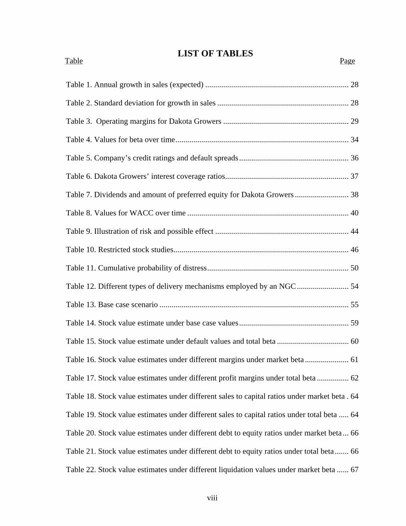
LIST OF TABLES
Table 1. Annual growth in sales (expected) ........................................................................ 28
Table 2. Standard deviation for growth in sales .................................................................. 28
Table 3. Operating margins for Dakota Growers ............................................................... 29
Table 4. Values for beta over time....................................................................................... 34
Table 5. Company’s credit ratings and default spreads ....................................................... 36
Table 6. Dakota Growers’ interest coverage ratios.............................................................. 37
Table 7. Dividends and amount of preferred equity for Dakota Growers ........................... 38
Table 8. Values for WACC over time ................................................................................. 40
Table 9. Illustration of risk and possible effect ................................................................... 44
Table 10. Restricted stock studies........................................................................................ 46
Table 11. Cumulative probability of distress....................................................................... 50
Table 12. Different types of delivery mechanisms employed by an NGC.......................... 54
Table 13. Base case scenario ............................................................................................... 55
Table 14. Stock value estimate under base case values....................................................... 59
Table 15. Stock value estimate under default values and total beta .................................... 60
Table 16. Stock value estimates under different margins under market beta ...................... 61
Table 17. Stock value estimates under different profit margins under total beta ................ 62
Table 18. Stock value estimates under different sales to capital ratios under market beta . 64
Table 19. Stock value estimates under different sales to capital ratios under total beta ..... 64
Table 20. Stock value estimates under different debt to equity ratios under market beta ... 66
Table 21. Stock value estimates under different debt to equity ratios under total beta ....... 66
Table 22. Stock value estimates under different liquidation values under market beta ...... 67
Table Page

ix
Table 23. Stock value estimates under different liquidation values under total beta .......... 68
Table 24. Annual sales growth (expected)........................................................................... 68
Table 25. Profit margins (expected) .................................................................................... 69
Table 26. Stock value estimate for a new issue under market beta ..................................... 70
Table 27. Stock value estimate for a new issue under total beta ......................................... 71

x
LIST OF FIGURES
1. Growth in equity for the cooperatives. ............................................................................1
2. Stock value estimates under different profit margins ....................................................62
Figure Page

1
CHAPTER I. INTRODUCTION
Background
Cooperatives play an important role in the economy. Even though cooperatives can
be found in every sector of the economy, they are most prevalent in agriculture. The
United States Department of Agriculture (USDA) reports that 3,466 farmer cooperatives
generated a net business volume of $115 billion for 1999. As illustrated in Figure 1,
cooperatives’ net worth (equity) amounted to $20 billion in 1999 (Kraenzle et al. 1999).
$10,000
$12,000
$14,000
$16,000
$18,000
$20,000
$22,000
1990 1991 1992 1993 1994 1995 1996 1997 1998 1999Year
Net
Wor
th (M
illio
n D
olla
rs)
Figure 1. Growth in equity for the cooperatives.
Historically cooperatives in the United States evolve in waves as a response to
market failures (Fulton 2001). In early 1900s, cooperatives emerged as a response to
oligopolistic markets that farmers faced. In the 1940s and 1950s, they emerged in public
utilities because urban service providers did not invest in the rural areas. Finally, in the

2
early 1990s, a new wave of the cooperatives materialized called New Generation
Cooperatives (NGCs). NGCs emerged as a result of structural changes in agriculture.
As agricultural food products continue to become more differentiated, traditional
relationships in the agricultural marketing channels undergo significant changes. Parties in
the channel become increasingly dependent on each other, and vertical integration and
contracting between producer and buyer replace traditional third-party transactions among
buyer, producer, and middleman. Also, retailers possess information about consumer
demand and translate that information down the channel telling farmers what to produce,
when, how much, and what quality. Information gives retailers power to dictate conditions
and the ability to shift risks to other parties in the channel, farmers in this case.
Requirements to produce specific products under certain conditions translate into
investments in specialized assets and create asset specificity problems. Asset specificity
problems arise when a producer is required to undertake a significant investment to create a
product tailored to one customer. Because tailored products have little market value and
cannot be sold without significant price concessions to another customer, a producer will
be reluctant to undertake this investment. Producing under these circumstances exposes a
supplier to the opportunistic behavior of the buyer. Because a specialized product cannot be
resold easily, the supplier will not produce unless a buyer demonstrates a significant
commitment to buy, such as a long-term contract. According to Fulton (2001), asset
specificity problems represent a market failure, and this failure helped lead to the creation
of NGCs.
An NGC is a cooperative with distinctive characteristics: ownership of shares tied
with delivery obligations of primary agricultural commodities, membership closed to
3
producers of the commodity, and tradable stock. The presence of the delivery obligation is
intended to address the asset specificity problem. The delivery obligation is similar to a
long-term contract. It assures farmers that the cooperative will buy their product as long as
the product meets specifications.
Also, characteristics of NGCs are designed to address problems of traditional
cooperatives. First, a closed membership cooperative solves the free-rider problem. Free
riders are non-members who benefit from cooperatives without incurring any membership
risk or contributing capital. Now, through NGCs, members accrue cost-reducing and
profit-enhancing benefits of a cooperative without sharing those benefits with non-
members.
Besides addressing problems of traditional cooperatives, NGCs bring additional
benefits. NGCs generally raise the income of farmers and increase employment in rural
areas. It is believed that a rural development strategy, a strategy to revive the state through
establishment of NGCs, is responsible for an 11 percent increase in disposable income
from 1990-1994 and an increase in manufacturing jobs by 3,500 (Stefanson, Fulton, and
Harris, 1995). Numerous studies, such as Bangsund and Leistritz (1998) and Stefanson,
Fulton, and Harris (1995), confirm that NGCs contribute jobs to local employment through
value-adding activities, thereby increasing the incomes of rural population and reducing
migration. For example, as summarized by Stefanson, Fulton, and Harris (1995), 300 jobs
were created in Carrington, where Dakota Growers Cooperative built its plant. Dakota
Growers contributed a $40 million investment to the local economy. In Volga, a plant built
by the South Dakota Soybean Processors Cooperative created 70 new jobs. Besides
contributing jobs, NGCs’ investments create positive externalities, thus boosting
4
construction, rural infrastructure, and the local tax base. It was estimated that the economic
impact of three sugar processing NGCs (American Crystal Sugar, Minn-Dak Farmers
Cooperative, and Southern Minnesota Beet Sugar Cooperative) was $831.1 million in fiscal
1997, $544.6 of which were payments to growers, that is in addition to 2,486 full–time
equivalent jobs created and 30,400 indirectly supported jobs (Bangsund and Leistritz,
1998).
Problem Statement
While there is evidence that NGCs have a positive impact on farmers and rural
communities, creation of and membership in NGCs often requires a substantial up-front
investment. Historically, NGCs have raised 30-50% of their capital needs through the sale
of stock (Stefanson, Fulton, and Harris, 1995). Because equity investment represents a
substantial portion of total financing, equity valuation becomes critical for management
and members of the cooperative.
Because the market for NGC stock is thinly traded, market valuation of NGC stock
is difficult and further complicated by the following factors. The pool of prospective
member-investors is limited to those who have the ability to provide commodities for
processing. First, the cooperative must treat its members fairly as input suppliers and as
investors. If the members do not feel they have been treated fairly as both input suppliers
(i.e., complex or burdensome delivery procedures) and investors (i.e., an unacceptable
return on investment), the cooperative will find it very difficult to raise additional equity
capital. Unlike conventional companies, NGCs’ shares have commodity delivery
obligations. This feature makes NGC stock unique and complicates valuation.
5
Financial characteristics of cooperatives make tracing equity flows complicated.
Cash flows from NGC stock comprise dividends and patronage. While dividends are
distributed fully in cash, the distribution of patronage is more complicated. Patronage has
two parts: cash and retained. Cash patronage is distributed to members in cash (hence the
name). Retained patronage is a non-cash portion of patronage that is retained by the
cooperative. The cooperative is liable to the members for the retained patronage. Therefore
each share of stock has a potential flow of cash with uncertain repayment timing. This
uncertain timing of retained patronage distribution is part of the stock’s value. Paying back
the retained portion may take several years (from 5 to 7), and during this time, the stock
may be sold several times. Tracking the retained patronage and determining its contribution
to the stock’s overall value complicates the valuation procedure.
Also, only face value is returned when retained patronage is distributed. NGC does
not pay interest on the original amount of patronage retained. Assuming stochastic interest
rates, the value of the retained patronage is uncertain. Economic theory says that the value
of the asset is the sum of all cash flows it is expected to generate discounted at the market
rate. In this case, the stream of cash flows has uncertain timing, which is further
complicated by changing interest rates. This uncertainty is the greatest challenge for
NGC’s stock.
After-tax obligations are different for NGC stocks. Returns from conventional
corporations get taxed at two levels: first at the corporate level as earnings and second at
the individual level as dividends, a phenomenon known as double taxation. Cooperatives
do not pay taxes on income as long as they distribute income back to members. The issues
6
of single versus double taxation result in valuation differences. This difference should be
accounted for in a stock valuation model.
Currently, no industry guideline is available for NGC management to reference
when valuing NGC stock. Corporate stock valuation procedures are a good starting point
for estimating NGC stock values. However, those models do not take into account the dual
responsibility of a cooperative member to invest equity capital and supply products while
valuing the uncertainty of retained patronage. The contribution of this study is to provide
analysis and guidelines regarding appropriate NGC stock valuation methods. The stock
valuation method employed will account for the thinly traded market and delivery
obligations imposed upon member/owners while more closely relating stock value to a
NGC’s stochastic returns.
Objectives
The objective of this study is to develop a stock valuation model that will be used to
appraise NGC equity. To accomplish this overall objective, the factors affecting NGC stock
value are identified and characterized. Procedures include reviewing literature and financial
statements of NGCs. Managerial insight about financial management is gained from
personal interviews with cooperative leaders and industry experts.
After determining the factors impacting NGC equity, a stock valuation simulation
model is developed. A Discounted Cash Flow (DCF) valuation tool is employed. The
impact of delivery requirements is incorporated in the model. Also, to account for thinly
traded markets, a liquidity discount is introduced. Furthermore, uncertainty is introduced
through stochastic simulation. Distributions for variables are obtained from the cooperative
and industry historical financial statements and data.
7
The stochastic model incorporates the variable distributions in a traditional present
value framework. Several scenarios are analyzed to determine sensitivities and address
issues such as
- An NGC uses different pricing strategies. For example, fixed pricing for American
Bison and prevailing market prices for Dakota Growers. These strategies have
different costs and benefits to members and their NGCs.
- The amount of reinvestments is subject to NGC management discretion.
Reinvestment is a cash outflow that is not immediately available to investors, thus it
reduces stock value under the DCF valuation method. While it may be tempting to
reduce reinvestment, it is not feasible because, if reinvestment is in a project with
positive NPVs, the reinvestment should enhance stock value. The enhancement in
the stock price is because reinvestment in favorable opportunities should raise
expected future rate of growth in dividends.
- Changes in profit margins are often the result of management decisions. Poor
management decisions may reduce profit margins. Superior thinking and a well-
devised strategy may improve the margins and enhance profitability.
- The capital structure of a cooperative is usually a result of management decision
making. However, choice of the debt and equity structure is vital for the company’s
long-term viability. An excessive amount of debt or a low level of equity will
reduce a cooperative’s flexibility and may lead to bankruptcy.

8
Organization
Chapter II provides an overview of the existing literature on cooperative and traditional
stock valuation models. Chapter III describes the model data and Methodology. Chapter IV
supplies Results, and Chapter V includes a discussion of the results, recommendation, and
outline for future research.
9
CHAPTER II. LITERATURE REVIEW
This project utilizes contributions from many research areas, such as cooperative
theory, bankruptcy, liquidity, cost of capital, risk, and valuation. More precisely, this work
applies modern financial valuation theory to the cooperative structure and NGCs. As such,
the following Literature Review presents research findings as they relate to the study.
Cooperative Theory and NGC
Cobia (1989) gives a comprehensive guide to cooperatives. He lists opportunities and
methods of capital accumulation for cooperatives, major debt providers, and credit policies.
He also mention ways cooperatives redeem equity. Taxation issues faced by cooperatives
are discussed, in particular taxation of refunds to the member and cooperative level and
additional deductions allowed to cooperatives under current tax code.
Stefanson et al. (1995), Stefanson and Fulton (1997), and Fulton (2001) provide a set
of factors in the current agricultural state that led to the development of NGCs. Definition
for NGCs is given together with a description of the challenges NGCs face and the benefits
they provide.
Chaddad and Cook (2002) analyzed the presence of financial constraints in
agricultural cooperatives. A reduced-form investment model was built utilizing data from
1991 to 2000. Investment demand was measured by Marginal q, where q is the present
value sum of future profits from an additional investment. Because Marginal q is not
observable, a proxy known as Fundamental q was used in the study. In addition to the
Marginal q, cash flows from the model were estimated. Parameters of cash flows, adjusted
for investment demand, from the model were analyzed to estimate the presence of the
financial constraints. Presence of financial constraints would be represented by positive and

10
significant cash flow parameter. The underlying assumption tested was that a financially
constrained company makes an investment only if it generates sufficient internal funds.
Alternatively, a company without financial constraints makes investment decisions
regardless of internal funds’ availability. The model was estimated by three different
methods: fixed effects (utilizing OLS), random effects, and generalized method of
moments estimators. It was concluded that cooperatives are, in fact, financially
constrained. This finding reinforces the importance of equity capital valuation for
cooperatives.
Sporleder and Bailey (2001) employed a real option valuation framework to value
investment into NGCs. The hypothetical situation where farmer-members of NGCs invest
into a food processing plant was modeled. To estimate payoff from the investment, a
dynamic simulation model was developed using the Black-Sholes real option pricing
formula. Authors integrate the concept of first mover advantage into the model by setting
values of time parameter and uncertainty parameter as a function of preemption.
Distribution of potential earnings per share served as an indicator of investment feasibility.
Investment was found to be feasible under several scenarios. The research illustrated
application of general financial valuation to the NGC investment. It also demonstrated how
risk considerations can be incorporated in the model.
Pederson (1998) described several possible approaches to estimate the cost of capital
for agricultural cooperatives. Pederson described two possible approaches that can be used
to estimate cost of capital for the agricultural cooperatives: accounting based and market
based. Market based incorporates the capital asset pricing model (CAPM), arbitrage-
pricing model (APT), and discounted cash flows (DCF). It is mentioned that accounting
11
approaches derive the cost of capital from the Constant Growth Model (CGM). He argues
that, in reality, due to the lack of the information and restrictive set of assumptions, only
two models are used, Option Pricing Model (OPM) or DCF. The advantages of OPM
include the use of both accounting (firm capital structure) and market data. One advantage
of DCF is its flexibility. The model allows, using different growth rates, cooperatives to
create wide ranges of values for the cost of capital. It was concluded that no single
approach can be used in finding the cost of capital.
Moller et al. (1996) identify and quantify sources of financial stress that
cooperatives face. They present an analytical method to measure the influence of each
factor that contributes to financial distress. Further stress is analyzed based on the
cooperative’s size and product mix. It is concluded that most stress results from low
earnings, high interest rates, and leverage. Also, small cooperatives are twice as likely to
suffer from distress as big cooperatives.
Delivery Obligation Mechanisms
Moore and Noel (1995) describes several agricultural cooperatives that operate
marketing pools. Unlike traditional marketing cooperatives, to be able to benefit from this
pool, members should have transferable delivery rights (TDR). The main purpose of
creating these rights is to increase liquidity by creating “a member property right based on
the contractual right to deliver commodity to the cooperative and to allow members a
limited right to sell and transfer the asset” (Moore and Noel, 1995).
When the cooperative establishes a pool, each member is required to deliver a certain
portion of the pool. If the cooperative is growing, each member’s share increases pro-rata.
If a member who has the TDR decides to exit farming or to change his crop mix, he can
12
sell his TDR. Over time, a secondary market where TDRs are sold and bought has
emerged. The survey was conducted among cooperative members. Unfortunately, the size
of sample was too small to apply statistical models, but two components of TDR’s value
have been identified: insurance value and premium value. An insurance value arises from
the fact that the member has a secured market for his crop. Because a cooperative signs a
long-term contract, it is obligated to buy the crop from the farmer.
The second component is called premium value because cooperative membership
entitles the farmer to receive patronage which would not be available otherwise. Thus, the
TDR’s value can be maximized if the cooperative attempts to provide both or at least one
of the values. The value of a TDR is a function of several variables, including industry
structure, producers’ behaviors toward production risks, and size of firms. It was concluded
that a TDR has value if membership is closed, if financial positions of the members
improved in the past with a TDR, if market power or barriers to entry possible, and if the
presence of insurance value and/or premium returns.
Equity Valuation, Free Cash Flows, Risk, and Cost of Capital
Much of the literature has been written on corporate stock valuation approaches.
Damodaran (2001) provides extensive description of different stock valuation models. He
reviews four models: Capital Asset Pricing Model (CAPM), Arbitrage Pricing Model
(APM), Multi-Factor Model (MFM), and Regression Model (RM). It is mentioned that all
models have two common assumptions: they define risk in terms of variance of returns and
argue that investment should be viewed from the standpoint of the marginal investor; the
last assumption translates in the underlying premise that investors are well diversified. This
assumption does not hold true for NGCs because farmers tend to not be well diversified.

13
Also, none of the models take into account the fact that investors are suppliers and that
delivery obligations are present. Adjustments for diversification and delivery obligations
are incorporated in the model presented in this study.
Among the existing cost of capital models, CAPM was used for valuation. The
major strength of APM, MFM, and RM is their reliance on several variables in explaining
risk. All models utilize regression analysis to explain risk, and from basic statistics, it is
known that more relevant variables produce a better fit. Unlike CAPM that utilizes only
one variable, APM, MFM, and RM utilize several variables. This feature was intended to
make these models superior to CAPM, but in our case, it was a weakness. First, as it was
mentioned, NGCs have weak secondary market; limited trading produces little, if any,
market information. Second, many NGCs are often young companies, so, in fact, no market
information is often available. Because CAPM utilizes only one variable, market premium,
CAPM output beta can be easily estimated and standardized among companies and
industries. Standardization of beta across industries and wide acceptance of betas as a
relevant valuation tool created benchmark industry betas that can be used to find the costs
of capital for any company as long as the company’s area of business is known, even if
individual cost of capital numbers are not available. This approach is utilized in the model
presented in this study.
Kaufold (1997) discusses two approaches to value a company: Adjusted Present
Value (APV) and Weighted Average Cost of Capital (WACC). Assuming different
scenarios of financial strategy, he shows that the two methods show identical results. He
concludes that APV should be used when the company targets the dollar level of debt and
WACC when the company plans to follow a fixed debt to value ratio.

14
Damodaran (1999) concentrates on risk-free rate estimation. Basic assumptions and
requirements are discussed for the asset to be risk free, and conditions for choosing the
appropriate risk-free rate for valuation are discussed. Also estimation of foreign country
default risk premiums is illustrated.
Booth (1999) discusses stimulation of the equity premium and equity costs. He
notes that the conventional approach to estimate equity cost was to look at it as a premium
over long-term bond yields. He identifies several biases associated with this approach. It is
concluded that excess equity return above long-term bonds cannot be used as a risk
premium and that bond yields have been increasing over the last 20 years and cannot be
assumed to be constant.
Pettit (1999) addresses issues of market premium estimation. He argues that, even
though equity premium over the past 40-50 years has exceed long term-bond yield by 5%,
this result may misleading because it ignores the systematic risk that bond yield
encompasses. He provides a method that allows adjusting beta for the bond yield risk and
also provides methods for better beta estimation.
Damodaran (2001) discusses the estimation of Free Cash Flows (FCF). He defines
FCF as a net income after reinvestments and net debt payments that is a net cash flow
available to equity holders. FCF importance arises from the fact that FCF potentially
represents cash flows that should be paid to investors in terms of dividends. Because net
income is often manipulated by different accounting procedures, Damodaran discusses
ways to adjust operating income, with emphasis given to adjusting for and amortization of
operating leases, managed earnings, and long-term expenses.
15
Jensen (1986) proposed that FCF carries agency costs. Because FCF is given back to
investors, FCF essentially reduces corporative funds at management disposal. These funds
are often misused by management who are biased toward company growth because growth
enhances compensation. Management has incentives to reinvest (rather than distribute to
shareholders) FCF into projects. Jensen shows that reinvestment occurs even if these
projects are not going to increase (and may even reduce) the company’s value. Jensen
argues that companies with significant FCF should replace their equity with debt because
interest payments, unlike dividends, are compulsory and must be repaid.
Mann and Sicherman (1991) discuss agency costs of FCF by expanding Jensen’s
argument. They suggest that shareholders expect management to reinvest FCF in
potentially unprofitable ventures conditional on past history of management. By studying
market response to equity announcements, they show that, if a company has a record of
related business acquisition, overall shareholder reaction is usually positive. If a company
has a record of making unrelated (thus potentially value-destroying) business acquisitions,
shareholder reaction is negative.
Damodaran (2001) addresses estimation of a firm’s terminal value. Two approaches
to calculate terminal value are discussed: liquidation value and stable growth value. When
the liquidation value approach is used, it is assumed that a company will cease its existence
and its assets will be sold at market prices at a given point of time. The weakness of this
approach is the ignorance of a going concern and goodwill. Under the stable growth
approach it is assumed that a company will grow forever at a constant rate, and Gordon’s
stock valuation formula is utilized to find a company’s worth. Because cooperatives are
assumed to have infinite lives, stable growth approach was utilized in the model presented.
16
Also, the stable growth approach is preferred because its use of liquidation value requires
more characterizing assumptions (state of economy, asset values, and inflation) than the
liquidation approach.
Liquidity Discount
An asset is said to be liquid when it can be bought or sold at the market price
quickly and at low cost. Amihud and Mendelson (1991) argued that, because investors are
risk averse, they require liquid assets. If an asset is not liquid, it should offer higher returns
than an otherwise similar liquid asset. Amihud and Mendelson use an equilibrium model
where assets are classified by their transaction costs, investors are classified by their
holding periods, and transaction costs are amortized over the investment period. Using beta
and the logarithm value of average bid-ask spread, a regression analysis was conducted.
Results showed that asset returns increase with illiquidity of an asset. In equilibrium, a
liquid asset will be traded more often, thus its transaction costs are incurred more often,
and its present value is lower while a less liquid asset is traded less frequently and has
higher return. Because returns are expressed as a percentage of the total value, returns are
lower for a more liquid asset.
Publicly traded companies often issue additional equity that is not registered with the
SEC and cannot be traded publicly. This unregistered equity, called restricted stock, is
placed privately at a discount. The discount is often used as a proxy for liquidity discount.
Courts often use results to appraise the value of the taxable assets. Research by Silber
(1991) illustrates the use of restricted stock prices. Silber provides a simple framework to
estimate liquidity discount. He identifies four variables, credit-worthiness of firm,
marketability, cash flow, and whether the investor is a client, as being crucial in estimating
17
liquidity discount. Next, Silber discusses proxies for the four. Silber’s results were
consistent with earlier studies of restricted securities and demonstrate that companies with
larger revenues and greater market capitalization have lower discounts.
Robak and Hall (2001) provide more detailed industry-level information on liquidity
discounts. Comprehensive statistical information is provided on liquidity discount, its
average, standard deviation, median, and discounts by the industry group.
Bankruptcy
Because the model utilizes bankruptcy probabilities, it is important to the discuss
literature on bankruptcy. The main emphasis in the bankruptcy research is placed on lender
use of credit scoring models. The main goal is to develop a system that will identify a
failing company. While the purpose of the present study is cursory to these models, it is
worth noting that several issues impact company/cooperative valuation. The general result
for many of the studies was the failing company can be predicted only at one to two years
prior to bankruptcy (Skadberg, 1985).
Different financial and accounting ratios are traditionally employed for analysis. The
most often used ratios are working capital/total assets, cash flow/total liabilities, current
assets/current liabilities, and working capital/sales. Rose and Gary (1984) show that only
two ratios, working capital/total assets and cash flow/total liabilities, demonstrate
predictive power. They conclude that bankruptcy analysis should include capital structure
and activity ratios to be useful in prediction.
Damodaran (2002a) illustrates how the probability of bankruptcy can be incorporated
in discounted cash flow valuation analysis. A company’s value can be treated as the
probability of weighted expected value of two components: going concern value and
18
liquidation value. A going concern value is defined as the sum of all cash flows discounted
at the respective WACC. He provides tables that allow estimating the probability of
bankruptcy based on a company’s interest coverage ratio.

19
CHAPTER III. METHODOLOGY
Rationale for Model
The goal of this research is to develop a model for NGC equity valuation. This
chapter describes assumptions and discusses the valuation model. The abundance of
financial information (financial statements) about cooperatives and the lack of market
information (market prices) prompted the choice of discounted cash flow valuation method
as the primary valuation tool for this research. The presented model is adapted from
Damodaran (2001) and modified to reflect the unique features of NGCs.
Model Description
The value of NGC stock is modeled as
CDLDNEVESV ±−= )1()( , (1)
where
SV = stock value,
E (EV) = expected equity value,
N = number of shares,
LD = liquidity discount, and
CD = cost of delivery obligation (may be positive or negative).
The model has four inputs, expected equity value, number of shares, liquidity
discount, and cost of delivery obligation. To illustrate model calculations, the Dakota
Growers (DG) NGC was chosen as an example. While no longer an NGC, DG was a
cooperative at the start of the thesis. (For explanations refer to the “Recent Developments”
section.) The number of shares for DG was obtained from annual 10-K statement.

20
Derivation of other inputs is discussed in the respective sections. Several model
assumptions are described below.
Assumptions
The first assumption is that all income is generated from patron business. This
assumption leads to a current tax rate of zero. Cooperatives, unlike conventional
corporations, have two sources of income, one with members and one with non-members.
Under current legislation, cooperatives do not pay taxes for conducting business with
member/owners, assuming all profits are distributed back to the member/owners.
Cooperative non-members’ income is subject to taxation. This clause makes valuation
more complicated because earnings before interest and taxes (EBIT) must be divided
between member and non-member business. Because non-member business is subject to
taxation, it has to be adjusted for taxes before it is added back to EBIT. Because
cooperatives are formed primarily to service members and NGCs (the focus of this study)
are closed membership cooperatives, revenues from business with non-members are
assumed to be a secondary (and relatively insignificant) source of revenue. Effectively by
introducing this assumption, it is assumed that all income is generated from business with
members and that the current tax rate is zero. This assumption not only simplifies the
model, but also reflects the reality of NGCs.
The second assumption is that the cooperative pays market price for inputs (i.e.,
wheat). This assumption is introduced so that the cooperative’s operating margin can be
approximated to the industry’s operating margin. If the cooperative pays higher than
market price, then one expects the cooperative’s operating margin to be lower because
higher prices increase the cost of goods manufactured and decrease profits. Decreased

21
operating margins are assumed to cause the equity value to drop. One has to bear in mind
that cooperatives are organized to benefit members, and management will accept lower
margins if members want the cooperative to pay higher than market prices. Similarly,
prices lower than the market increase operating margins and increase equity value. The
market price assumption is also important because industry financial ratios are used as a
financial benchmark for the cooperative. The benchmark ratios are derived from industry
corporate financial statements. These companies buy inputs at market prices, but NGCs
may not. If the cooperative decides to deviate from market price, its operating profit
margins are different. This assumption is relaxed in further analysis.
A third assumption is that only one type of NGC stock is issued. Corporations issue
different classes of equity. Each type has distinctive features and unique value.
Cooperatives usually issue two types of equity, voting stock and shares with delivery
obligation. Voting stock is limited to one share per member, and there is no delivery
obligation. To simplify valuation, this study assumes one kind of equity that entitles
members to claim cash flows from the cooperative. This type of stock includes delivery
obligations. Because NGCs require membership closed to farmers who can deliver a
primary agricultural input, this assumption follows reality.
The fourth assumption relates to the credit ratings table that is used in the model. The
credit rating table used in the model is from Damodaran (2002a). The credit coverage ratio
is used as a proxy for credit worthiness of the company. The credit coverage ratio in this
study is defined as operating income divided by interest expense. This table relies on credit
ratings used by credit rating agencies in order to define the probability of default. It is
assumed in the model that credit rating agencies provide realistic credit assessment. If
22
credit companies do not have realistic credit assessment, then the probability of bankruptcy
and default rate does not reflect true probability of bankruptcy and default. If credit ratings
change over time, then the probability of bankruptcy vary from year to year for the same
company.
The fifth assumption is that the cooperative does not change its debt to equity mix,
i.e., it remains constant. While constant mix is a simplifying assumption, it is not far from
reality. Usually, a company’s debt to equity mix may vary but usually within a specific
range. Lending agencies require cooperatives to finance at least 50% of their investment
capital as equity investment (Olson, 2002), so debt equity mix may have bounds fixed by
lenders. There is a limited investor pool, where farmers may be reluctant to infuse
additional equity. Identification of the range is an empirical matter, but if the cooperative
has been in business for 7-10 years (i.e., past the initial start-up phase of the cooperative),
its current debt to equity mix is assumed to be fairly steady.
It is also assumed that the current credit rating is assumed to be fairly steady. Lenders
traditionally specify a range of ratios that lending agencies monitor closely. In this study,
ratios, such as interest coverage ratio, have a lower bound. If a cooperative’s ratio drops
lower than specified by the lender, the lender intervenes. The lender may demand an
immediate repayment of the loan, forcing the company into involuntary bankruptcy.
Because this action will limit the cooperative and management’s flexibility in running the
business, managers avoid violating these ratios unless the cooperative is under severe
financial distress, thus automatically requiring bankruptcy. The probability of bankruptcy is
incorporated in the model. Alternatively, an improvement in these ratios indicates a better
financial position and is favored by lenders. If ratios improve, the lender may reduce the
23
interest rate, thus changing the cost of capital and equity value of the cooperative. If the
company is already in good financial standing (BBB or higher) when signing a lending
agreement, like Dakota Growers, a decrease in the lending rate may be insignificant (up to
1% decrease) in relation to the overall weighted cost of capital. The impact will depend on
the proportion of debt in the cooperative’s capital structure, but with imposed borrowing
limitations, the impact is likely to be insignificant. If the company originally had a poor
credit rating, then a change in equity value is likely to be significant.
Liquidity discount is assumed to be 23%. DG belongs to the group of industries with
a standard classification code (SIC) of 2000. According to Robak and Hall (2001), an
average discount for industry with SIC of 2000 is 23%. Operating income is adjusted for
operating leases. All operating leases are treated as capital leases. Both operating and
capital leases represent the same type of commitment (Damodaran, 2001). All debt is
assumed to be nonconvertible. While DG does have convertible debt, the portion of
convertible debt in regard to the total amount of capital is insignificant. This assumption is
introduced to simplify valuation.
Annual sales growth rate and risk-free rate are assumed to be underlying sources of
uncertainty in the model. Both of them are assumed to be normally distributed. Because
nominal interest rates cannot take negative values, normal distribution, which is used to
generate values for interest rates, is truncated at 0.05%. This number is assumed to be the
lowest value that an interest rate can take. Means and standard deviations are estimated
from historical data for respective variables. Also, their correlation is estimated and
incorporated in the model. The remaining variables are assumed to be non-stochastic.
24
The cooperative may only cease to exist due to bankruptcy liquidation. It is assumed
that any feasible business entity, a cooperative in this case, will not be dissolved for other
reasons. This assumption is stated explicitly because the model incorporates only
probabilities of bankruptcy while, in reality, any cooperative may dissolve voluntarily. It is
reasonable to expect that farmers will not dissolve the cooperative as long as they can
benefit from it. Analysis is conducted using nominal interest rates and sales growth in real
terms.
Company beta approaches one during the transition period and is equal to one in the
constant growth period (Damodaran, 2001). In the long run, any company is as risky as the
market itself. Therefore a company’s beta will approach one as it matures.
Equity Valuation Model
Equity value is estimated as the weighted average of discounted total cash flows
(TCF) that are expected from the cooperative as going concern (multiplied by the
probability of the cooperative staying in business) and liquidation value (multiplied by the
probability of the cooperative going bankrupt). TCF calculation is adopted from
Damodaran (2000) and is expressed as
nn
nt
tt
t
WACCTV
WACCFCFFE
TCF)1()1(
)(1 +
++
= ∑=
=
, (2)
where
TCF = total cash flows,
TV n = expected terminal value of the company calculated at year n,
WACC = weighted average cost of capital,
t = number of high growth years (transition period),
n= beginning of constant growth (end of transition period), and

25
E (FCFF) = expected free cash flows to the firm (FCFF) for high growth period.
Mature vs. Young Firm and Constant vs. High Growth
Because the current model utilizes Gordon’s stable growth valuation model, several
key issues have to be discussed. For a complete coverage of Gordon’s stable growth model,
see Ross et al. (1988). A company is said to be mature if it meets all three conditions listed
below.
First, the company is capable of sustaining sales growth at the industry average into
perpetuity. Second, it is capable of delivering returns on capital close to industry average
returns in perpetuity. Third, its reinvestment rate approaches the industry average
reinvestment rate. It is assumed that any young company will become mature or go
bankrupt. Because the probability of bankruptcy is accounted for in the model, the issue of
maturity is of interest. More precisely, the point at which a young company becomes
mature is of importance. It is important because young companies earn excess returns while
mature companies do not. The length between a base year and the beginning of a constant
growth period is a transition period. During the transition period, a young company
transforms into a mature company. It is during this period when a company’s excess
returns disappear. The length of this transition period reflects expectations about a
company’s ability to earn excess returns for a period of time. Therefore, length of transition
period or presence of excess return is the same concept and is interchangeable. Also, it is
during this transition period when a young company enjoys a high (above industry average)
growth, so it is during the high growth period when a company earns excess returns. At the
end of a transition period, a young company becomes mature and grows at a constant
26
(industry average) rate. These concepts are discussed in greater details in the Framework
for Industry Analysis section.
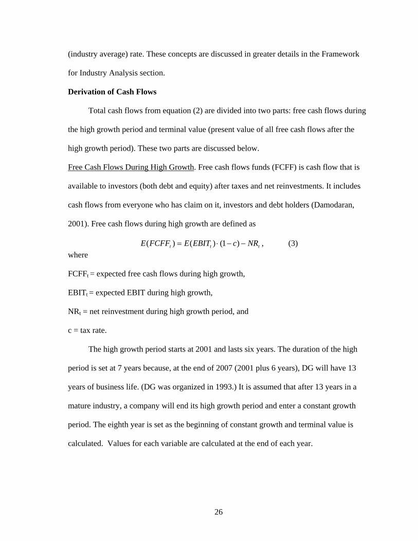
Derivation of Cash Flows
Total cash flows from equation (2) are divided into two parts: free cash flows during
the high growth period and terminal value (present value of all free cash flows after the
high growth period). These two parts are discussed below.
Free Cash Flows During High Growth. Free cash flows funds (FCFF) is cash flow that is
available to investors (both debt and equity) after taxes and net reinvestments. It includes
cash flows from everyone who has claim on it, investors and debt holders (Damodaran,
2001). Free cash flows during high growth are defined as
ttt NRcEBITEFCFFE −−⋅= )1()()( , (3) where
FCFFt = expected free cash flows during high growth,
EBITt = expected EBIT during high growth,
NRt = net reinvestment during high growth period, and
c = tax rate.
The high growth period starts at 2001 and lasts six years. The duration of the high
period is set at 7 years because, at the end of 2007 (2001 plus 6 years), DG will have 13
years of business life. (DG was organized in 1993.) It is assumed that after 13 years in a
mature industry, a company will end its high growth period and enter a constant growth
period. The eighth year is set as the beginning of constant growth and terminal value is
calculated. Values for each variable are calculated at the end of each year.

27
Because calculations in the model for Dakota Growers (DG) start at 2001, the initial
value for EBIT is DG EBIT for 2001. Subsequent values for EBIT (from 2002 to 2008) are
found by applying the following formula:
ttt OPSalesEEBITE ⋅= )()( , (4) where
E (Salest) = expected sales in year t and
OP = operating profit margin (gross profit after marketing, general and administrative
expenses divided by gross sales).
The figure for the sales for the first year (2001) is obtained from the income
statement and equal to $173,467. The initial sales growth figure is obtained as a weighted
average of the previous three years growth (1998, 1999, and 2000) and equal to 11%. Sales
values are derived from the following equation:
)1()( 1 ttt gSalesSalesE += − , (5)
where
gt = expected growth in sales.
Annual sales growth percentage during the transitional period is shown in Table 1.
Gradually, initial sales growth of 11% is lowered to the industry average growth of 6%.
The industry growth is calculated as a 30-year average of annual growth in the value of
shipments. Industry sales growth is obtained from the Annual Survey of Manufacturers
(ASM) using the value of industry shipment as a proxy for industry sales; the time period
used is from 1970 to 2000. It is common for start-ups to grow faster than a mature
company, but this growth is not sustainable in the long run. It is assumed that, in the long
run, the company will not grow faster than the industry.
28
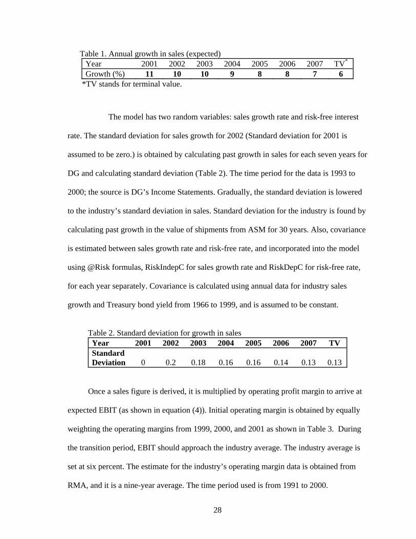
Table 1. Annual growth in sales (expected) Year 2001 2002 2003 2004 2005 2006 2007 TV* Growth (%) 11 10 10 9 8 8 7 6
*TV stands for terminal value.
The model has two random variables: sales growth rate and risk-free interest
rate. The standard deviation for sales growth for 2002 (Standard deviation for 2001 is
assumed to be zero.) is obtained by calculating past growth in sales for each seven years for
DG and calculating standard deviation (Table 2). The time period for the data is 1993 to
2000; the source is DG’s Income Statements. Gradually, the standard deviation is lowered
to the industry’s standard deviation in sales. Standard deviation for the industry is found by
calculating past growth in the value of shipments from ASM for 30 years. Also, covariance
is estimated between sales growth rate and risk-free rate, and incorporated into the model
using @Risk formulas, RiskIndepC for sales growth rate and RiskDepC for risk-free rate,
for each year separately. Covariance is calculated using annual data for industry sales
growth and Treasury bond yield from 1966 to 1999, and is assumed to be constant.
Table 2. Standard deviation for growth in sales
Year 2001 2002 2003 2004 2005 2006 2007 TV Standard Deviation
0
0.2
0.18
0.16
0.16
0.14
0.13
0.13
Once a sales figure is derived, it is multiplied by operating profit margin to arrive at
expected EBIT (as shown in equation (4)). Initial operating margin is obtained by equally
weighting the operating margins from 1999, 2000, and 2001 as shown in Table 3. During
the transition period, EBIT should approach the industry average. The industry average is
set at six percent. The estimate for the industry’s operating margin data is obtained from
RMA, and it is a nine-year average. The time period used is from 1991 to 2000.

29
Table 3. Operating margins for Dakota Growers
Year 2001 2002 2003 2004 2005 2006 2007 TV Operating Margin (%)
6
6
6
6
6
6
6
6
Usually start-ups have a different profit margin than the industry operating margin.
As a company matures, its operating margin approaches the industry average. During the
transition period, this operating margin must approach the industry average, and in the long
run, it must stay equal to it. If it is consistently lower than the industry average, the
company will not be able to exist in the long run. Assuming a higher than average
operating margin is also not feasible because competition will erode high operating
margins in the long run. Higher than average margins are possible if there are barriers to
entry, such as high switching costs and/or patents.
There is a slightly different scenario for DG. DG had excellent timing for entry.
Because of good timing, this company was able to find its niche and earn higher than
average operating profit margins from inception. DG has faced new entrants. Other
companies were able to enter and cause DG’s operating margins to fall.
Net Reinvestment During High Growth. The next input in equation (3) is net reinvestment
(NR). NR is important for valuation because it represents cash outflow and reduces cash
flows available for investors. It is important to set NR realistically because low or
inadequate NR will hinder a company’s long-term growth and decrease future operating
margins. Net reinvestment for the base year is obtained from the 2001 financial statements
for DG as net capital expenditures (capital expenditures minus depreciation) plus the
change in non-cash working capital (working capital minus cash).
30
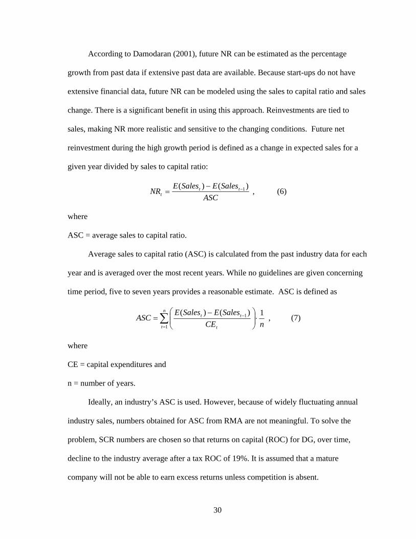
According to Damodaran (2001), future NR can be estimated as the percentage
growth from past data if extensive past data are available. Because start-ups do not have
extensive financial data, future NR can be modeled using the sales to capital ratio and sales
change. There is a significant benefit in using this approach. Reinvestments are tied to
sales, making NR more realistic and sensitive to the changing conditions. Future net
reinvestment during the high growth period is defined as a change in expected sales for a
given year divided by sales to capital ratio:
ASCSalesESalesE
NR ttt
)()( 1−−= , (6)
where
ASC = average sales to capital ratio.
Average sales to capital ratio (ASC) is calculated from the past industry data for each
year and is averaged over the most recent years. While no guidelines are given concerning
time period, five to seven years provides a reasonable estimate. ASC is defined as
∑=
− ⋅⎟⎟⎠
⎞⎜⎜⎝
⎛ −=
n
t t
tt
nCESalesESalesE
ASC1
1 1)()( , (7)
where
CE = capital expenditures and
n = number of years.
Ideally, an industry’s ASC is used. However, because of widely fluctuating annual
industry sales, numbers obtained for ASC from RMA are not meaningful. To solve the
problem, SCR numbers are chosen so that returns on capital (ROC) for DG, over time,
decline to the industry average after a tax ROC of 19%. It is assumed that a mature
company will not be able to earn excess returns unless competition is absent.
31
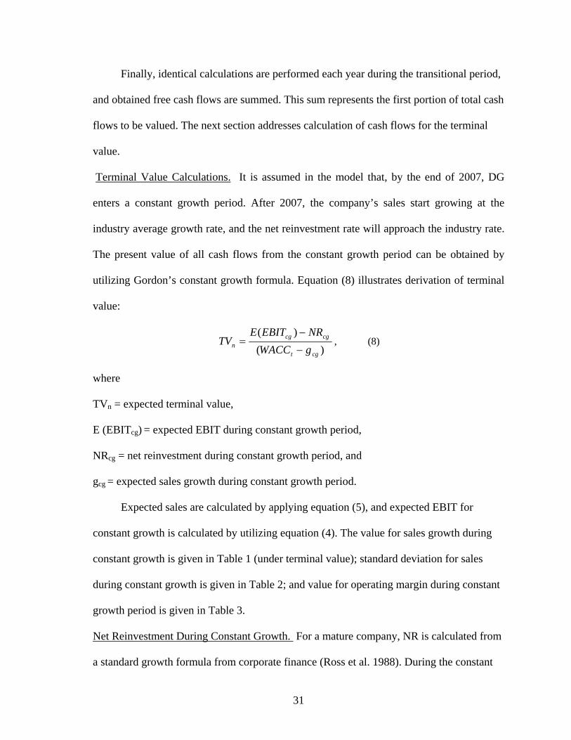
Finally, identical calculations are performed each year during the transitional period,
and obtained free cash flows are summed. This sum represents the first portion of total cash
flows to be valued. The next section addresses calculation of cash flows for the terminal
value.
Terminal Value Calculations. It is assumed in the model that, by the end of 2007, DG
enters a constant growth period. After 2007, the company’s sales start growing at the
industry average growth rate, and the net reinvestment rate will approach the industry rate.
The present value of all cash flows from the constant growth period can be obtained by
utilizing Gordon’s constant growth formula. Equation (8) illustrates derivation of terminal
value:
)()(
cgt
cgcgn gWACC
NREBITETV
−
−= , (8)
where
TVn = expected terminal value,
E (EBITcg) = expected EBIT during constant growth period,
NRcg = net reinvestment during constant growth period, and
gcg = expected sales growth during constant growth period.
Expected sales are calculated by applying equation (5), and expected EBIT for
constant growth is calculated by utilizing equation (4). The value for sales growth during
constant growth is given in Table 1 (under terminal value); standard deviation for sales
during constant growth is given in Table 2; and value for operating margin during constant
growth period is given in Table 3.
Net Reinvestment During Constant Growth. For a mature company, NR is calculated from
a standard growth formula from corporate finance (Ross et al. 1988). During the constant
32
growth period, NR is assumed to be constant for every year and is set as a percentage of
EBIT. This percentage number is derived from the following formula:
)( cgcg
cgcg EBITE
ROCg
NR ⎟⎟⎠
⎞⎜⎜⎝
⎛= , (9)
where
NR cg = net reinvestment during constant growth year,
g cg = expected growth in sales during constant growth period,
ROC cg = return on capital during constant growth period, and
E (EBITcg) = expected EBIT during constant growth period.
Net reinvestment during constant growth finalizes the calculation of terminal value
of the company, the second portion of total cash flows. Next section will discuss derivation
of WACC.
Calculation of Risk Parameters for Equity Valuation
Because FCFF in the model represents future cash flows, it must be discounted. The
rate should reflect the company risk. Weighted Average Cost of Capital (WACC) is used to
reflect inherent risks. WACC is computed as the weighted average of costs from three
sources of capital: cost of equity, cost of debt, and cost of preferred equity.
pepeddee kWkWkWWACC ⋅+⋅+⋅= , (10)
where
WACC = weighted average cost of capital,
We = proportion of equity as percentage of total capital,
ke = equity cost,
Wd = proportion of debt as percentage of total capital,

33
kd = cost of debt,
Wpe = proportion of equity as percentage of total capital, and
kpe = cost of preferred equity.
Calculation of Equity Costs
The first component of capital is equity. Equity is a major source of capital for
agricultural cooperatives. Cooperative members commit a significant up-front investment.
Members’ investments represent a substantial portion of new investment financing for
NGCs. Cost of member equity is computed using the CAPM model (Ross et al., 1988).
RPbkk adjrfe ⋅+= , (11)
where
ke = equity cost,
krf = risk-free rate, 10-year Treasury Bonds rate minus the historic average risk premium of
10-year bond over 1-year Treasury bill rate,
badj = beta adjusted for leverage and diversification, and
RP = market risk premium.
Damodaran (2001) estimated that historic risk premium equals four percent. Because
DG is not a publicly traded company, beta for the company was not available. As a proxy,
beta for American Italian Pasta (AIP) was obtained. It is assumed that companies with
similar product mix and in similar markets, such as AIP, should have similar betas. This
beta is a market beta; it is not adjusted for leverage or for diversification. Beta for AIP is
equal to 0.65 in 2001. The beta value is increased by 0.05 per year until reaching 1. It is
assumed (See Assumptions.) that, in the long run, the company’s beta will approach 1 (i.e.,
company becomes as risky as the market) (Table 4).

34
Table 4. Values for beta over time
Year 2001 2002 2003 2004 2005 2006 2007 TV Beta 0.65 0.65 0.7 0.75 0.8 0.85 0.9 1
Beta is further adjusted for leverage. Beta is modified for leverage as
)1(EDMBbml += , (12)
where
bml = market beta adjusted for leverage,
MB = unlevered market beta, and
D/E = debt to equity ratio.
Debt and equity values in the ratio are market values. The reasons for using market
values are discussed below.
The CAPM model assumes that the investor is well diversified and that beta only
measures market risk, i.e., risk that cannot be diversified. While an institutional investor
may be well diversified, a farmer is not. Beta in such cases should be adjusted. Damodaran
(2001) suggests adjusting as
PiS
MBTB
&σ= , (13)
where
TB = total beta and
PiS &σ = correlation between industry and market index (Standard and Poor in this case).
35
Total beta is further adjusted for leverage
)1(EDTBbtl += , (14)
where
btl = total beta adjusted for leverage and diversification.
The range between leverage adjusted market beta and total beta represents the risk
range that investors in the cooperative face. An institutional investor will have a beta close
to the market beta because an institutional investor is better diversified than an individual
investor. Individual betas for farmers will be close to the total beta. Also, individual betas
will vary among farmers because one farmer may be better diversified than another. Two
scenarios are assumed in the model; the first one is for investors who have a beta equal to
the market beta, and the second is investors whose beta are equal to the total beta. An
equity value will be calculated in each scenario. The value depends on the level of
diversification of individual investors. The base case scenario assumes that investors are
fully diversified and uses market beta adjusted for leverage as in equation (11).
In addition, the present values of operating lease commitments are added to the total
debt. It is assumed that operating leases represent the same commitment as capital leases,
so operating lease commitments are part of the debt in this study.
Calculation of the Cost of Debt
Cost of debt is calculated using the interest coverage ratio. Damodaran (2002b)
suggests that cost of debt can be estimated from several sources. Synthetic rating is one
way to estimate the cost of debt. Recent borrowings can serve as an indicator of a
company’s credit standing as well. If the company to be valued is a large, publicly traded
company, credit-rating agencies most likely have already rated it. The rating simplifies

36
valuation because all that needs to be done in this case is to find a representative risk-free
rate and add a corresponding default spread. New start-ups, small companies, and closely
held companies are not typically rated. In these cases, when estimating a synthetic rating,
one assumes the role of a credit rating agency. To rate a company in this case, the
following steps may be performed. First, an interest coverage ratio is chosen as an indicator
of the company’s cost of debt. The interest coverage ratio is important because it measures
the company’s ability to make interest payments on time, and the ratio is also correlated
with other ratios specified in the master loan agreement (Damodaran, 2002a). The change
in the interest coverage ratio is indicative of interest repayment capacity and of changes in
other debt ratios. Table 5 reports default spread for companies based on their interest
coverage ratio. It uses the S&P credit rating system to rate a company’s creditworthiness.
Table 5. Company’s credit ratings and default spreads Interest Coverage Ratio Rating Spread
(%) Default Rate
(%) > 8.5 AAA 0.20 0.01
6.5 - 8.5 AA 0.50 0.03 5.5 - 6.5 A+ 0.80 0.40 4.25 - 5.5 A 1.00 0.53 3.0 - 4.25 A- 1.25 1.41 2.5 - 3.0 BBB 1.50 2.3 2 - 2.5 BB 2.00 12.2
1.75 – 2 B+ 2.50 19.3 1.5 - 1.75 B 3.25 26.4 1.25 - 1.5 B- 4.25 32.5 .8 - 1.25 CCC 5.00 46.6 .65 - .8 CC 6.00 65.0 0.2 - .65 C 7.50 80.0 < 0.65 D 10.00 100.0
Source: Damodaran (2002a).
37
To calculate the cost of debt, the default spread is added to the corresponding risk-
free rate. For example, a credit rating for DG is assigned based on an interest coverage ratio
estimated from past and current financial statements.
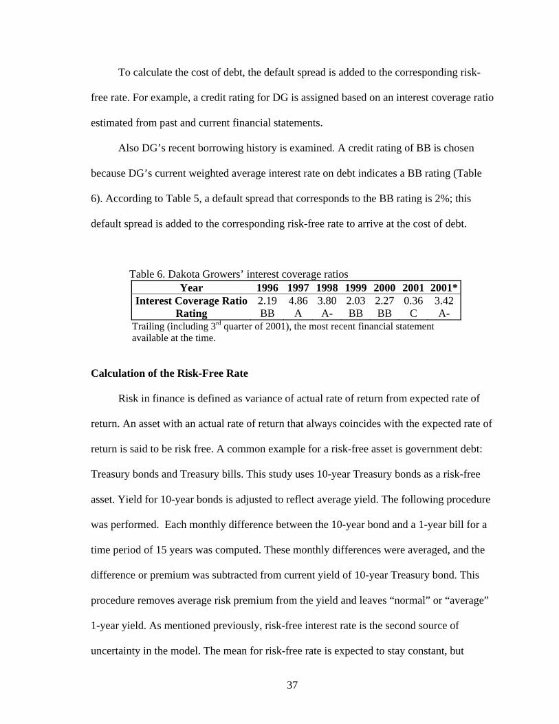
Also DG’s recent borrowing history is examined. A credit rating of BB is chosen
because DG’s current weighted average interest rate on debt indicates a BB rating (Table
6). According to Table 5, a default spread that corresponds to the BB rating is 2%; this
default spread is added to the corresponding risk-free rate to arrive at the cost of debt.
Table 6. Dakota Growers’ interest coverage ratios Year 1996 1997 1998 1999 2000 2001 2001*
Interest Coverage Ratio 2.19 4.86 3.80 2.03 2.27 0.36 3.42 Rating BB A A- BB BB C A-
Trailing (including 3rd quarter of 2001), the most recent financial statement available at the time.
Calculation of the Risk-Free Rate
Risk in finance is defined as variance of actual rate of return from expected rate of
return. An asset with an actual rate of return that always coincides with the expected rate of
return is said to be risk free. A common example for a risk-free asset is government debt:
Treasury bonds and Treasury bills. This study uses 10-year Treasury bonds as a risk-free
asset. Yield for 10-year bonds is adjusted to reflect average yield. The following procedure
was performed. Each monthly difference between the 10-year bond and a 1-year bill for a
time period of 15 years was computed. These monthly differences were averaged, and the
difference or premium was subtracted from current yield of 10-year Treasury bond. This
procedure removes average risk premium from the yield and leaves “normal” or “average”
1-year yield. As mentioned previously, risk-free interest rate is the second source of
uncertainty in the model. The mean for risk-free rate is expected to stay constant, but

38
changes can be easily incorporated. However, covariance with sales growth rate is
incorporated in the value of risk-free rate in each year. Standard deviation for the risk-free
rate is calculated from the monthly yields (time period February 1990 to February 2000)
for the Treasury bonds and is equal to 0.01.
Cost of Preferred Equity
The last component of the WACC is cost of preferred equity. Dakota Growers has
three types of preferred stock: Series A, B, and C. Weighted average interest on preferred
stock is calculated using inputs shown in Table 7, and it is equal to 5%.
Table 7. Dividends and amount of preferred equity for Dakota Growers
Amount
Dividend Yield (%) Par Value
Weights(%)
Series A 600 6 100 29 Series B 525 2 100 26
Series C (Convertible) 925 6 100 45 Total 2050 5 - 100
Calculation of Weights for Capital Cost Components
Finally, all three costs are weighted by market values and summed up together. The
market values are used because they reflect true values of equity and debt: “use of market
values is justified by the fact that the cost of capital measures the cost of issuing securities
stocks and bonds to finance projects, and these securities are issued at market value, not at
book value” (Damodaran, 2001, pp. 43-44). Also, the use of market values concentrates on
the money-generating ability of the asset (i.e., Company is viewed as going concern.); it
makes the model more realistic and approximates the value better.
Market value of equity is obtained by taking the total number of shares and
multiplying by current stock price. Use of current stock price to find a stock price may
39
appear to be confusing. However, one has to bear in mind that it is market value of equity
as a whole, not the market price of an individual share, that is used here. Market value for
equity is important as one of the inputs to the model. If market prices are not available,
there are other ways to compute market value. One can look at the publicly traded
companies with a similar product mix and develop a proxy, a coefficient that will allow for
computing the market values of private companies. However, this approach requires
analytical methods that may deviate from the main focus of this study. Another approach to
find the market value of equity is by taking the market price of stock (if available) and
multiplying it by the number of shares. This research utilizes the second approach due to
time and resource constraints. Approaches to finding market values of equity for WACC
purposes can be refined continuously, and calculation of market value is merely a detail.
Calculation of debt market value is somewhat complicated. Large, publicly traded
companies have publicly traded debt. In this case the market value of debt can be obtained
similarly to the market value of equity. If the company is small and/or start-up, it will not
have publicly traded debt. In this case, treating debt as one large bond can approximate the
market value of debt. Coupon payment of the bond is an interest expense; face value is the
total amount of debt principal; discount rate is the cost of debt that was assigned according
to the rating; and time to maturity is the average of all maturities weighted by principal.
WACC Calculation and Operating Value of Asset
Once all inputs for equation (12) are calculated, WACC is obtained by weighting and
summing. Because beta increases (Table 3) over years and other components of WACC
stay the same (See Assumptions.), the value of WACC increases over time (Table 8).
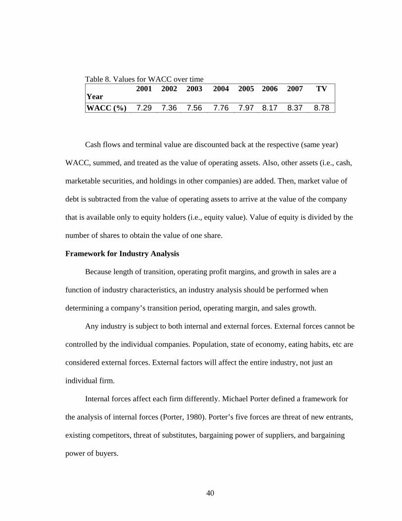
40
Table 8. Values for WACC over time
Year 2001 2002 2003 2004 2005 2006 2007 TV
WACC (%) 7.29 7.36 7.56 7.76 7.97 8.17 8.37 8.78
Cash flows and terminal value are discounted back at the respective (same year)
WACC, summed, and treated as the value of operating assets. Also, other assets (i.e., cash,
marketable securities, and holdings in other companies) are added. Then, market value of
debt is subtracted from the value of operating assets to arrive at the value of the company
that is available only to equity holders (i.e., equity value). Value of equity is divided by the
number of shares to obtain the value of one share.
Framework for Industry Analysis
Because length of transition, operating profit margins, and growth in sales are a
function of industry characteristics, an industry analysis should be performed when
determining a company’s transition period, operating margin, and sales growth.
Any industry is subject to both internal and external forces. External forces cannot be
controlled by the individual companies. Population, state of economy, eating habits, etc are
considered external forces. External factors will affect the entire industry, not just an
individual firm.
Internal forces affect each firm differently. Michael Porter defined a framework for
the analysis of internal forces (Porter, 1980). Porter’s five forces are threat of new entrants,
existing competitors, threat of substitutes, bargaining power of suppliers, and bargaining
power of buyers.
41
Threat of new entrants is an important factor. New entrants will increase supply, and
unless consumer demand for a product increases faster than the increase in supply,
increased supply will drive consumer prices down. Barriers to entry and expected
retaliation are two factors which will prevent new entrants from entering the market (Hitt
et al., 1999).
Existence of barriers to entry depends on the following factors: economies of scale,
product differentiation, switching costs, access to distribution channels, and government
policy. As a company increases output, it gains economies of scale. The presence of
economies of scale indicates large capital requirements, giving advantage to incumbent
firms and preventing new firms from entering. If already an incumbent in the market with
significant barriers to entry and the company in valuation earns excess returns, one can
expect these returns to persist in the future. Also, transition period in this case would be
longer than if barriers were not present or not significant. Operating margins would be
above average operating margins as well.
Skillful product differentiation may create an image of the company’s product as
being unique (Hitt et al., 1999). This perception will give a company the ability to
command higher prices and enjoy higher than average profit margins. The presence of
successful product differentiation will increase the transition period.
Switching costs are defined as costs a customer bears when switching to a different
supplier. If switching costs are high, consumers will be reluctant to change supplier.
Switching costs are not always expressed in dollar terms; they can be in terms of time
commitment or individual preferences. The company that manages to create switching
42
costs has enormous advantage over companies that do not have them. Such a company will
be able to charge higher prices and will have more stable sales in the future.
In some industries, vertical integration is prevalent. In this case, a new entrant will
have to create its own distribution channel. The creation of distribution channels is
expensive and risky. Lack of access to the distribution network, thus, can be an effective
deterrent for new companies. Operating margins and transition period for the incumbent
firm would be larger in markets with limited access.
Another important deterrent for new entry discussed by Hitt et al. (1999) is expected
retaliation. If companies in an industry are known to retaliate, new entrants will be
reluctant to enter the market. In this case, an incumbent company may enjoy a longer
transition period and above average operating margins.
Bargaining power is an important factor in defining the length of transition period
and operating margins. Porter (1980) differentiates bargaining power of both buyers of a
company’s products and input suppliers to the company. Suppliers and buyers have
separate economic goals. Buyers minimize the purchase costs by obtaining the lowest
possible prices, and suppliers maximize profits by obtaining the highest possible prices.
During negotiations, parties try to maximize their objectives at each others’ expense. It is a
win-lose situation, and the party with greater bargaining power wins. If a valued company
has greater bargaining power, it will enjoy higher operating margins and is capable of
earning excess returns longer.
The threat of substitute products is likely to affect an entire industry. The appearance
of new substitutes and the presence of old ones will decrease the sales growth rate during
the transition and stable growth periods, ultimately affecting operating margins.
43
The existing rivals also influence the transition period and operating profit margins
through competition (Hitt et al., 1999). Industries with a large number of competitors tend
to be more competitive than the industries with a smaller number. Industry growth is also
an important determinant of intra-industry rivalry. The slower the growth, the more
aggressive rivals will be. Excess supply will often result in fierce price competition,
bringing prices down.
As suggested by Damodaran (2001), in addition to the industry factors discussed,
company factors should be considered. Size of the firm is important. Small firms are more
likely to earn excess returns because small firms grow faster in the market than large
companies. Small company transition period should be set longer than for a large company.
Company size should be considered relative to the industry’s stage. If an industry is in a
growth stage, then even a large company will be able to grow fast.
Past growth and earnings should be considered. If a company has made excess
earnings for the last five years, it is likely to continue earning excess returns. For a
company with superior profitability and impressive historic growth, the transition period
should be longer than for a company that does not possess similar achievements.
It is also worth noting that top management can be crucial in defining the transition
period. Historically, success stories of CEOs who have made excellent strategic decisions
that impacted not only the company, but the entire industry, are known industry-wide
(Damodaran, 2001). The quality of the management team should be taken into account in
defining the margins and transition period.
Illustrating what has been discussed so far, let us consider Dakota Growers. DG
operates in a mature industry with slow growth. Its dependence on several major industrial

44
accounts indicates a lack of bargaining power, making DG vulnerable to the opportunistic
behavior of its customers. It also manufactures a product which is not differentiated, with
low if any switching costs. Some economies of scale are present, but access to distribution
channels is not restricted. These factors will shorten DG’s transition period and more
quickly eliminate excess returns for DG. Currently, there is government intervention
against importers of pasta as a result of anti-dumping action. This positive factor will
potentially lengthen the transition period and excess returns.
In fact, risks and uncertainties that companies report to investors in SEC filings and
which management faces every day can be analyzed and adjusted in the model. Many, if
not all, management risks ultimately will impact sales, growth in sales, and operating
margins. While DG did not delineate the risks it is facing in the SEC statements, analysis of
an annual statement for American Italian Pasta (company similar in product mix to DG)
helps to describe the risks present for any company in the industry. How each of them may
affect sales growth, returns, or operating margins is illustrated in Table 9.
Table 9. Illustration of risk and possible effect
Risk Possible Effect
Dependence on several major customers Greater buyer power may possibly decrease operating profit margins and transition period.
Cost increases in inputs, i.e., durum wheat in packaging material.
Lower operating profit margins
Possible difficulty in managing growth
Slower growth rates and, as a result shorter transition period
Market for pasta is extremely competitive.
Slower growth rates and smaller operating profit margins

45
Liquidity Discount Estimation
An asset is said to be liquid if it can be sold at the current market price quickly and at
low cost (Amihud and Mendelson 1991). Because membership in an NGC is limited to
farmer-producers of a certain commodity, not everybody can invest in the cooperative.
There is limited demand for the shares; as a result, limited trading and illiquidity
characterize the secondary market for NGC equity. Therefore, adjustment is made to
account for a lack of liquidity. To address this problem, the liquidity discount came from
restricted stock studies.
Restricted stock studies have been used to measure liquidity of corporate equity.
Publicly traded companies issue stock that is not registered with SEC called letter stock or
restricted stock. The only difference between restricted and non-restricted stock is that
restricted stock cannot be publicly traded. Restricted stock is placed privately, and the
investor cannot resell it in the near future. The difference in price between restricted and
publicly traded stock gives an approximation of what the liquidity discount should be.
Because the liquidity discount depends on each company and varies from situation to
situation, it is likely to be different for each company. However, there are important
characteristics that Robak and Hall (2001) and Damodaran (2001) found that influence
liquidity discount. Several characteristics include asset liquidity, financial well being,
dividends, placement, and company size. Each characteristic is discussed briefly.
The extent to which assets in the company are liquid impacts liquidity discount.
Intuitively, the more cash or near-cash assets a company has, the easier it is to liquidate the
company’s assets at market price.

46
Profitable companies capable of generating a stable income will be worth more and
can be sold easier than a similar company in poor financial health.
Dividend-paying companies tend to have lower liquidity discounts. The dividends
provide an investor with funds, thus easing investor need for liquidity. Also, the larger the
dividend, the larger the amount of funds an investor is getting.
There is a negative correlation between size of placement and discount. Demand for
shares is elastic, so as quantity of shares (placement size) goes up, the price of stock goes
down. As the price of stock goes down, liquidity discount widens, or increases.
A company with larger sales will have lower liquidity discounts. A negative
relationship between sales and liquidity discount may be attributed to risk. Bigger
companies (with large sales) are perceived to be less risky. Therefore, their stock is more
liquid, and their liquidity discounts are smaller.
Robak and Hall (2001) list liquidity discounts by SIC codes, and the dry pasta
industry belongs to the industry group with SIC code 2000. Industries with SIC code 2000
have liquidity discount of 23%, with a standard deviation of 15% and median of 18.4%.
Robak and Hall summarize several restricted stock studies. Those studies are given in
Table 10.
Table 10. Restricted stock studies Restricted Stock Study Years Covered Average Discount
Institutional Investor Study 1966-1969 25.8% Gelman 1968-70 33.0% Trout 1968-72 33.5%
Moroney Not Specified 35.6% Maher 1969-73 35.4%
Standard Research Consultants 1978-82 45.0% Willamette Management Associates 1981-84 31.2%
Silber 1981-88 33.8%

47
Damodaran (2001) mentions that a rule of thumb for setting liquidity discounts is 20
to 30% of equity value. The discount chosen in this model is 23%, and stock value after
discount in the spreadsheet reflects the value of the stock after discount.
Finally, several other factors present in cooperatives impact liquidity. Investors are
risk averse, so sellers of an illiquid asset have to compensate buyers for purchase. The
compensation usually comes in terms of higher returns (Amihud and Mendelson, 1991).
Premium for liquidity is translated to higher cost of capital for the issuers of a financial
asset. By making the asset more liquid, the company will be able to reduce its cost of
capital. Therefore, it is in the best interest of the NGC to make its equity shares as liquid as
possible. Several ways of improving liquidity have been suggested in the financial
literature, including going public, reducing informational asymmetry, and paying regular
dividends (Amihud and Mendelson, 1991). Going public will increase the stock’s liquidity
by providing a larger number of potential buyers. Insuring that as much information as
possible is available to the public will reduce information asymmetry and increase
liquidity. Also, it is suggested that the presence of dividends increases liquidity, so regular
dividends are crucial to stock liquidity.
In the case of NGCs, there may be delivery obligations tied to stock ownership. If the
delivery obligation represents a cost to the stockholder, then the delivery obligation is a
source of illiquidity. Costly delivery obligations will reduce the number of potential
investors. Because delivery obligations may reduce potential investors, the cooperative
should reduce these delivery costs. All of these measures can be utilized to increase
liquidity, possibly increase demand, and boost equity value.

48
Probability of Bankruptcy
Throughout this study, the calculations assume an ongoing entity with infinite life. In
real life, there is no guarantee that a company will remain in business forever. In fact, there
is no guarantee that a company will remain in business until next year. Any company may
cease to exist due to bankruptcy. While a cooperative can be dissolved voluntarily, it is
assumed (in this study) that any feasible business venture will not be dissolved.
Bankruptcy is said to exist when total liabilities of the company exceed a fair value
of the company (Skadberg, 1985). Two possible consequences for a bankrupt company
include reorganization and liquidation. While it is possible for company to continue to exist
after reorganization, it ceases to exist after liquidation.
Economic and financial risks define the probability of a company going bankrupt
(Levy and Sarnat, 1982). Economic risk is a function of the external environment and is
taken as given. Financial risk, on the other hand, depends on the financial leverage of the
company. Financial structure is governed by management decision, so management is
responsible for financial risks. Interest and principal repayments are fixed expenses, and
because earnings are variable in nature, any fixed payments increase the chances of
bankruptcy. Thus, the larger the fixed payments, the higher the chances of bankruptcy
(Rose and Gary, 1984). The first 10 years of business existence are critical. It is during
these 10 years that a company is likely to go bankrupt. Altman (1971) reports that about
one-third of all bankruptcies take place in the first 3 years, 53% take place in the first 5
years, and the number increases to 70% for the first 10 years.
49
NGCs have additional factors making them more susceptible to risk. NGCs are
incorporated with the idea of processing a particular type of commodity. Thus, they are
restricted in their ability to diversify business activities.
Also, cooperatives have been known to face capital constraints that conventional
companies do not. There are different reasons for the presence of these constraints. For
example, farmers may view the cooperative as a secondary source of investment, with
primary investment being their farms. Illiquidity of the NGCs’ stock and uncertainty with
retained patronage payments may prompt member reluctance to supply additional financial
capital. The capital constraint problem is further aggravated by the fact that banks require
a minimum equity investment before lending. The inability to obtain funds from members
will limit the cooperative’s ability to obtain funds from lending institutions.
To make the model more realistic and adjust for the problems listed, the probability
of bankruptcy is incorporated. Probabilities are adopted from Damodaran (2001). The
probabilities are cumulative and assigned based on the credit rating of the company. Table
11 shows probabilities of a company going bankrupt for the next five and for the next ten
years.
In this study, liquidation value needs to be calculated to determine expected stock
value. In reality, liquidation value is subject to uncertainty because it is a function of
numerous variables, including location, state of economy, type of business, type of
equipment, industry conditions, etc. (Damodaran, 2002a). Because liquidation value cannot
be known in advance, simulations are run for several values of liquidation value ranging
from 10 to 100% of the total asset book value.
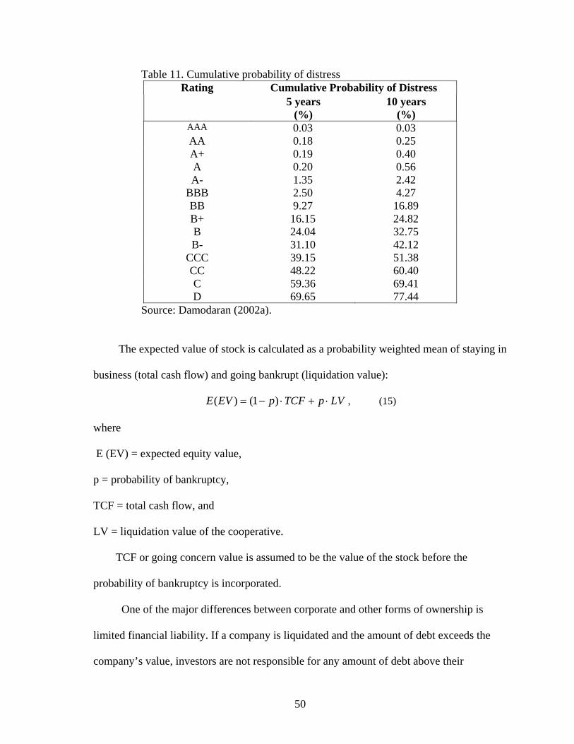
50
Table 11. Cumulative probability of distress Rating Cumulative Probability of Distress
5 years (%)
10 years (%)
AAA 0.03 0.03 AA 0.18 0.25 A+ 0.19 0.40 A 0.20 0.56 A- 1.35 2.42
BBB 2.50 4.27 BB 9.27 16.89 B+ 16.15 24.82 B 24.04 32.75 B- 31.10 42.12
CCC 39.15 51.38 CC 48.22 60.40 C 59.36 69.41 D 69.65 77.44
Source: Damodaran (2002a).
The expected value of stock is calculated as a probability weighted mean of staying in
business (total cash flow) and going bankrupt (liquidation value):
LVpTCFpEVE ⋅+⋅−= )1()( , (15)
where
E (EV) = expected equity value,
p = probability of bankruptcy,
TCF = total cash flow, and
LV = liquidation value of the cooperative.
TCF or going concern value is assumed to be the value of the stock before the
probability of bankruptcy is incorporated.
One of the major differences between corporate and other forms of ownership is
limited financial liability. If a company is liquidated and the amount of debt exceeds the
company’s value, investors are not responsible for any amount of debt above their
51
investment. Limited liability is incorporated in the model for reality. If the value of debt is
larger than the liquidation value, the model sets stock value to zero.
Cost of Delivery Obligation
Cost of delivery obligation (COD) is the last part of the stock valuation model. COD
is a unique component of the stock value present only in an NGC’s shares. COD can be
either negative (decreasing stock value) or positive (increasing stock value). If cooperative
membership results in certain extra costs, COD is negative. For example, wheat-processing
cooperatives often require members to grow more expensive, specific crop varieties. If the
cooperative refuses to buy the commodity (sometimes due to quality concerns), the farmer
may be forced to sell the crop on the open market at a substantial discount. Livestock
cooperatives may require members to produce highly specialized products which can be
sold on the open market only at a significantly reduced price. Members may also be
required to change their production practices as a part of becoming an NGC member.
These changes may add up to a significant cost to the member and affect stock value. In
addition to affecting stock value directly, COD will affect the stock’s value indirectly.
Costly COD will reduce the number of potential investors and will impact stock liquidity.
Cooperatives may need to create measures to reduce COD effects.
Although NGC membership may include some COD risks, being a member may
result in significant benefits for a farmer. Some cooperatives may pay transportation costs,
as Dakota Growers does. Also, if there is no well-established market for a particular
commodity, being a member of a cooperative that processes this commodity is of great
benefit for a farmer. The NGC, in this case, assumes part of the producer’s risk of selling
and marketing the commodity. For example, members of American Crystal Sugar

52
Cooperative (ACSC) benefit from being part of a cooperative because there is no open
market for sugarbeets. By purchasing sugarbeets from members and transforming them
into sugar, ACSC shares the risks of sugar production and marketing. It would be logical to
expect COD to be positive in this and similar cases.
Because COD is a function of producers’ costs, calculation of COD is specific to
each individual cooperative. Each cooperative operates in a different industry and has
specific production methods, often unique to the particular cooperative, particular industry,
and particular farmer. Nevertheless, common denominators can be easily identified, such as
storage costs, transportation costs, existence of a primary market for the commodity, and
existence of specific production requirements. Management and members should be able to
estimate the COD based on cooperative experience and access to data.
COD for DG is small, if any. From analyzing DG’s marketing agreement, it is clear
that transportation costs are paid by the cooperative. The grade of durum required by DG is
easily marketable on the open market at current market price. The only expense identified
is storage cost.
Initially, storage costs were modeled as a triangular probability distribution, with the
left border equal to zero and the right border equal to the largest storage cost possible. The
largest storage cost was identified as the largest holding of stock with the associated
delivery schedule. Because one share has the delivery obligation of one bushel, the member
with the largest amount of shares would have the largest storage costs. DG does not have a
restriction on the number of shares an individual member can hold. The current largest
holding is equal to 3% of the total number of shares. From subsequent phone conversations
with DG’s administration, it becomes clear that the cooperative can buy the number of
53
bushels associated with this number (i.e., 3% of total) in one day, so storage costs are not
significant in this case.
However, there is cost associated with not having commodity on hand. If the
cooperative requires delivery of durum and farmers cannot deliver, DG contacts Northern
Grain Institute (NGI). NGI is a nonprofit organization engaged in buying and delivering
commodity on behalf of members. It charges the member client $0.015 per bushel as a
service fee. In fact, as DG administration indicated, purchase of wheat by NGI on behalf of
members is common practice for some members. Some farmers sell durum at harvest and
then contact NGI to supply durum on member behalf when needed by DG. The service fee
is treated as COD and subtracted from the stock value in the model.
Table 12 illustrates several examples of possible delivery mechanisms (DM) that are
employed by NGCs (Olson, 2002). Costs are in comparison to the farmer who is a producer
of the same commodity but not a member of the cooperative.
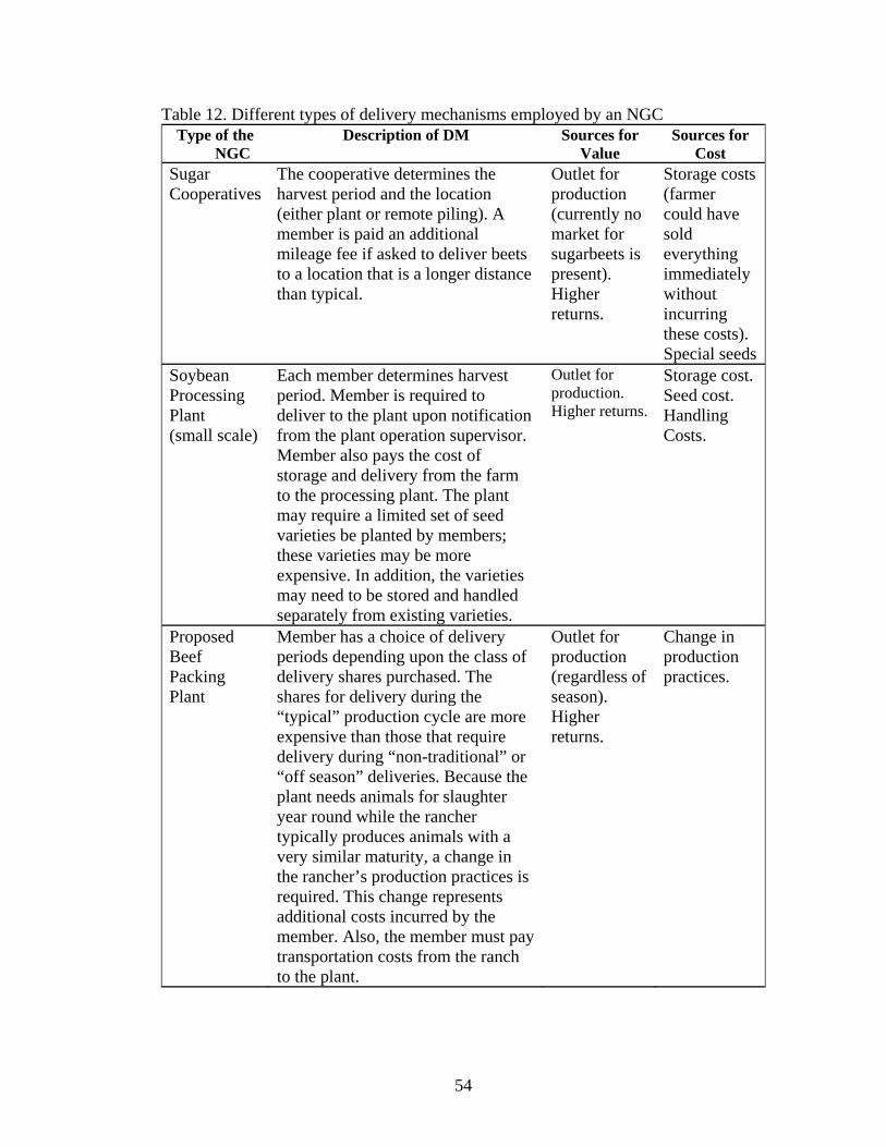
54
Table 12. Different types of delivery mechanisms employed by an NGC Type of the
NGC Description of DM Sources for
Value Sources for
Cost Sugar Cooperatives
The cooperative determines the harvest period and the location (either plant or remote piling). A member is paid an additional mileage fee if asked to deliver beets to a location that is a longer distance than typical.
Outlet for production (currently no market for sugarbeets is present). Higher returns.
Storage costs (farmer could have sold everything immediately without incurring these costs). Special seeds
Soybean Processing Plant (small scale)
Each member determines harvest period. Member is required to deliver to the plant upon notification from the plant operation supervisor. Member also pays the cost of storage and delivery from the farm to the processing plant. The plant may require a limited set of seed varieties be planted by members; these varieties may be more expensive. In addition, the varieties may need to be stored and handled separately from existing varieties.
Outlet for production. Higher returns.
Storage cost. Seed cost. Handling Costs.
Proposed Beef Packing Plant
Member has a choice of delivery periods depending upon the class of delivery shares purchased. The shares for delivery during the “typical” production cycle are more expensive than those that require delivery during “non-traditional” or “off season” deliveries. Because the plant needs animals for slaughter year round while the rancher typically produces animals with a very similar maturity, a change in the rancher’s production practices is required. This change represents additional costs incurred by the member. Also, the member must pay transportation costs from the ranch to the plant.
Outlet for production (regardless of season). Higher returns.
Change in production practices.

55
Base Case
This section summarizes the chapter by providing a table with model variables and
base values for these variables (Table 13). These values are used to compute a base case
scenario from which sensitivities can be analyzed.
Table 13. Base case scenario
2001 2002 2003 2004 2005 2006 2007 TV Revenue
Growth (%) 11 10 10 9 8 8 7 6
Standard Deviation for
Revenue
0
0.2
0.18
0.16
0.16
0.14
0.13
0.13
Operating margin (%) 6 6 6 6 6 6 6 6
Sales to Capital Ratio 2.7 2.7 2.7 2.7 2.7 2.7
Market Beta 0.65 0.65 0.7 0.75 0.8 0.85 0.9 1 Levered
Market Beta 1.2 1.2 1.3 1.4 1.4 1.5 1.6 1.6 Debt/Equity
Ratio (%) 78.4 78.4 78.4 78.4 78.4 78.4 78.4 78.4
Cost of Equity (%) 8.4 8.6 8.9 9.3 9.6 10.0 10.4 10.4
Cost of Debt (%) 5.80 5.85 5.85 5.85 5.85 5.85 5.85 5.85
Cost of Preferred Debt (%) 5.00
5.00
5.00
5.00
5.00
5.00
5.00
5.00
Treasury Bonds Yield
(TBY) (%) 3.85 3.85 3.85 3.85 3.85 3.85 3.85 3.85 Standard
Deviation for TBY 0.01 0.01 0.01 0.01 0.01 0.01 0.01 0.01
WACC (%) 7.29 7.36 7.56 7.76 7.97 8.17 8.37 8.37
Discount 23 % Liquidation
Value 20 % Bankruptcy Probability 17 %
Delivery Cost ($)
0.015
56
Use of @Risk for Sensitivities
The model incorporates risk through the use of @Risk. The final result of the
simulation that @Risk reports is an average value of all results it calculated during a given
number of iterations. In other words, for each iteration, @Risk assigns random values
according to the probability distribution specified and calculates the result. Then, it
averages results over n number of iterations and reports it as a final value. Also, @Risk has
a built-in function, RiskSimTable, that allows running simulations for different variable
values. RiskSimTable is used to derive sensitivities of the stock values.
Recent Developments
DG was originally chosen for this study because of several factors. First, the
company was in the high growth phase, and seven to eight years of financial data are
available. The presence of a high growth phase is important to illustrate the application of
the model. Second, the company explicitly states dividends on its financial statements,
unlike American Crystal Sugar (ACS). Also, the market price for the input (i.e., durum
wheat) is publicly available unlike the market price for sugarbeets. However, during
completion of the thesis, DG members voted on May 23, 2002, to convert from a
cooperative to a publicly traded corporation. Its conversion was completed by July 1, 2002.
In order to maintain its quality control over input and an image for farmers, DG decided to
create series D Delivery Preferred Stock (DPS). Owners of DPS will have privilege to
deliver durum for processing into pasta first.
Two main reasons are citied for the conversion: availability of durum wheat from
members and capital constraints (Rural Cooperatives, 2002). Durum production has fallen
dramatically in North Dakota, primary due to the scab disease. This decline in production

57
made DG input (i.e., wheat) procurement extremely difficult and threatened the DG
cooperative status. To be a cooperative, DG is obligated to buy at least 51% of its input
from members. One can argue that DG had no choice but to change its status because of the
difficulties with wheat procurement from the members.
Another argument for conversion to a public corporation is lack of capital.
Proponents of conversion argued that a change in status will increase the number of
investors and, thus, will bring more capital to the company.
There are several important factors that may affect the company as a result of the
conversion. On the positive side, DG may benefit from a lower cost of capital, either from
a lower cost of debt and/or a lower cost of equity. Lower cost of debt will be primary
because of debt’s tax advantage. Lower cost of equity will be primary because of better
access to the capital markets and to the larger number of investors. An additional important
benefit is stock liquidity which may decrease the cost of capital as well.
On the negative side, there are tax obligations. Because cooperatives do not pay
taxes, DG enjoyed tax-exempt status. After turning into a corporation, DG will be obligated
to pay taxes. Also, initially, the company may experience higher cost on the procurement
side because members are no longer obligated to deliver wheat. There are other minuses;
for example, many farmers perceive DG as being cooperative where members support and
help each other (Pates, 2002). With the conversion, the company will lose its “co-op
image” and become just any other corporation.
58
Summary
The model presented employs the DCF valuation tool to estimate stock price. This
chapter described steps and procedures for valuation. First, equity value is calculated, and
the value of equity per share is obtained. Second, a liquidity discount is applied to the value
of equity. Third, delivery cost/benefit is added/subtracted from the value of equity. Results
of the model are presented and discussed in Chapter IV.
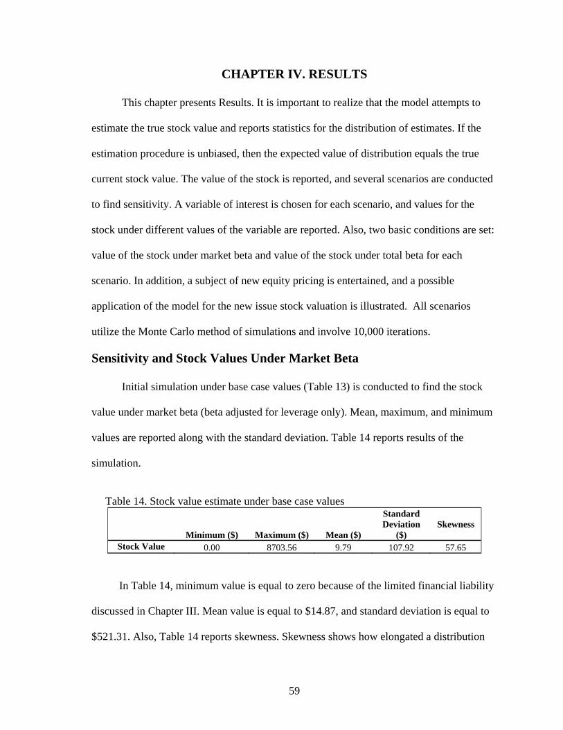
59
CHAPTER IV. RESULTS
This chapter presents Results. It is important to realize that the model attempts to
estimate the true stock value and reports statistics for the distribution of estimates. If the
estimation procedure is unbiased, then the expected value of distribution equals the true
current stock value. The value of the stock is reported, and several scenarios are conducted
to find sensitivity. A variable of interest is chosen for each scenario, and values for the
stock under different values of the variable are reported. Also, two basic conditions are set:
value of the stock under market beta and value of the stock under total beta for each
scenario. In addition, a subject of new equity pricing is entertained, and a possible
application of the model for the new issue stock valuation is illustrated. All scenarios
utilize the Monte Carlo method of simulations and involve 10,000 iterations.
Sensitivity and Stock Values Under Market Beta
Initial simulation under base case values (Table 13) is conducted to find the stock
value under market beta (beta adjusted for leverage only). Mean, maximum, and minimum
values are reported along with the standard deviation. Table 14 reports results of the
simulation.
Table 14. Stock value estimate under base case values
Minimum ($) Maximum ($) Mean ($)
Standard Deviation
($) Skewness
Stock Value 0.00 8703.56 9.79 107.92 57.65
In Table 14, minimum value is equal to zero because of the limited financial liability
discussed in Chapter III. Mean value is equal to $14.87, and standard deviation is equal to
$521.31. Also, Table 14 reports skewness. Skewness shows how elongated a distribution
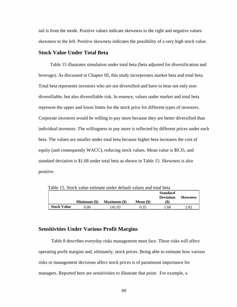
60
tail is from the mode. Positive values indicate skewness to the right and negative values
skewness to the left. Positive skewness indicates the possibility of a very high stock value.
Stock Value Under Total Beta
Table 15 illustrates simulation under total beta (beta adjusted for diversification and
leverage). As discussed in Chapter III, this study incorporates market beta and total beta.
Total beta represents investors who are not diversified and have to bear not only non-
diversifiable, but also diversifiable risk. In essence, values under market and total beta
represent the upper and lower limits for the stock price for different types of investors.
Corporate investors would be willing to pay more because they are better diversified than
individual investors. The willingness to pay more is reflected by different prices under each
beta. The values are smaller under total beta because higher beta increases the cost of
equity (and consequently WACC), reducing stock values. Mean value is $0.35, and
standard deviation is $1.68 under total beta as shown in Table 15. Skewness is also
positive.
Table 15. Stock value estimate under default values and total beta
Minimum ($) Maximum ($) Mean ($)
Standard Deviation
($) Skewness
Stock Value 0.00 141.03 0.35 1.68 2.82
Sensitivities Under Various Profit Margins
Table 8 describes everyday risks management must face. These risks will affect
operating profit margins and, ultimately, stock prices. Being able to estimate how various
risks or management decisions affect stock prices is of paramount importance for
managers. Reported here are sensitivities to illustrate that point. For example, a
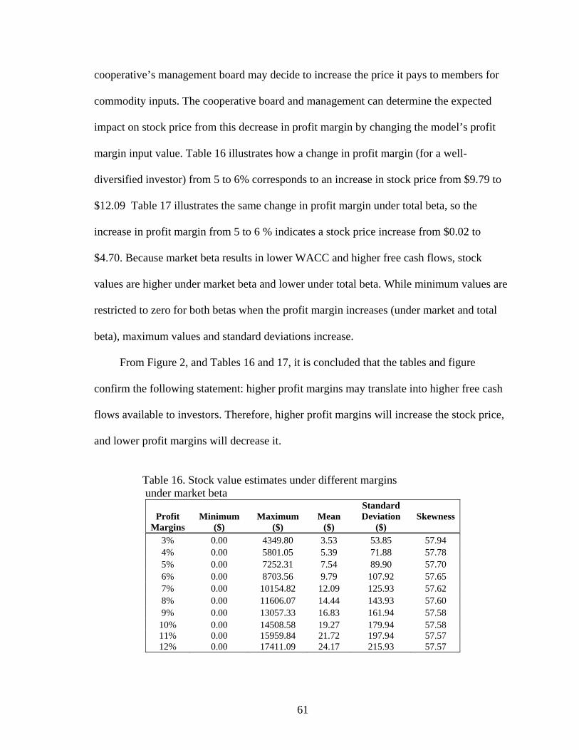
61
cooperative’s management board may decide to increase the price it pays to members for
commodity inputs. The cooperative board and management can determine the expected
impact on stock price from this decrease in profit margin by changing the model’s profit
margin input value. Table 16 illustrates how a change in profit margin (for a well-
diversified investor) from 5 to 6% corresponds to an increase in stock price from $9.79 to
$12.09 Table 17 illustrates the same change in profit margin under total beta, so the
increase in profit margin from 5 to 6 % indicates a stock price increase from $0.02 to
$4.70. Because market beta results in lower WACC and higher free cash flows, stock
values are higher under market beta and lower under total beta. While minimum values are
restricted to zero for both betas when the profit margin increases (under market and total
beta), maximum values and standard deviations increase.
From Figure 2, and Tables 16 and 17, it is concluded that the tables and figure
confirm the following statement: higher profit margins may translate into higher free cash
flows available to investors. Therefore, higher profit margins will increase the stock price,
and lower profit margins will decrease it.
Table 16. Stock value estimates under different margins under market beta
Profit Margins
Minimum ($)
Maximum ($)
Mean ($)
Standard Deviation
($) Skewness
3% 0.00 4349.80 3.53 53.85 57.94 4% 0.00 5801.05 5.39 71.88 57.78 5% 0.00 7252.31 7.54 89.90 57.70 6% 0.00 8703.56 9.79 107.92 57.65 7% 0.00 10154.82 12.09 125.93 57.62 8% 0.00 11606.07 14.44 143.93 57.60 9% 0.00 13057.33 16.83 161.94 57.58 10% 0.00 14508.58 19.27 179.94 57.58 11% 0.00 15959.84 21.72 197.94 57.57 12% 0.00 17411.09 24.17 215.93 57.57
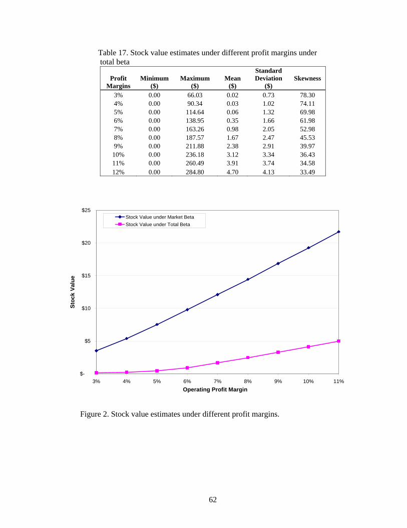
62
Table 17. Stock value estimates under different profit margins under total beta
$-
$5
$10
$15
$20
$25
3% 4% 5% 6% 7% 8% 9% 10% 11%Operating Profit Margin
Stoc
k Va
lue
Stock Value under Market BetaStock Value under Total Beta
Figure 2. Stock value estimates under different profit margins.
Profit Margins
Minimum ($)
Maximum ($)
Mean ($)
Standard Deviation
($) Skewness
3% 0.00 66.03 0.02 0.73 78.30 4% 0.00 90.34 0.03 1.02 74.11 5% 0.00 114.64 0.06 1.32 69.98 6% 0.00 138.95 0.35 1.66 61.98 7% 0.00 163.26 0.98 2.05 52.98 8% 0.00 187.57 1.67 2.47 45.53 9% 0.00 211.88 2.38 2.91 39.97
10% 0.00 236.18 3.12 3.34 36.43 11% 0.00 260.49 3.91 3.74 34.58 12% 0.00 284.80 4.70 4.13 33.49

63
Sensitivity Under Various Sales to Capital Ratios
As previously discussed, the average sales to capital ratio (ASC) is a proxy for future
net reinvestments. Knowing ASC and next year’s sales allows estimating the cooperative’s
reinvestment amount. Because net reinvestment (NR) is an investment, it reduces current
cash flows to (hopefully) increase cash flows in the future. It is tempting for management
to reduce NR, but an inadequate amount of reinvestments will decrease the cooperative’s
profitability and its long-term growth.
In Tables 18 and 19, a relationship between ASC and stock values is reported. It is
assumed that there is a change in ASC for the entire industry. This assumption is needed
for simplicity. If only DG increases ASC, thus increasing its investment in assets, then its
profit margin may increase. Investment in assets may make DG more competitive, thus
improving its profit. Because there is no benchmark to gauge how one firms’s investment
will change its profit margin relative to the industry, a change in ASC is treated as an
industry trend.
There is an inverse relationship between change in ASC (as industry trend) and stock
price. As net reinvestments increase, free cash flows go down, and so do stock values. This
finding is illustrated in Tables 18 and 19 under market and total betas. As ASC increases
from 2.5 to 3.5, stock value under market beta increases from $9.70 to $10.02 and stock
value under total beta increases to $0.53 from $0.29. Changes in values are smaller for
stock values under market beta. Minimum value is restricted to zero while maximum value
and standard deviation are stable. Skenwess is positive, implying that the distribution is
skewed to the right.
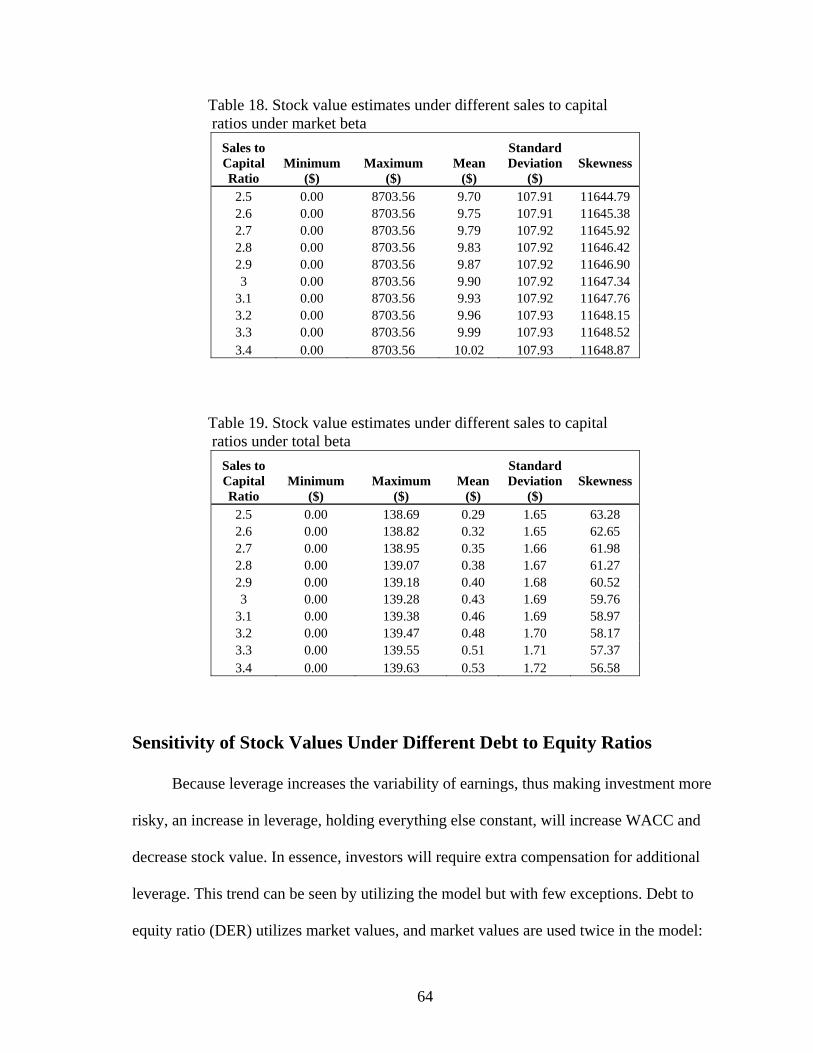
64
Table 18. Stock value estimates under different sales to capital ratios under market beta
Sales to Capital Ratio
Minimum ($)
Maximum ($)
Mean ($)
Standard Deviation
($) Skewness
2.5 0.00 8703.56 9.70 107.91 11644.79 2.6 0.00 8703.56 9.75 107.91 11645.38 2.7 0.00 8703.56 9.79 107.92 11645.92 2.8 0.00 8703.56 9.83 107.92 11646.42 2.9 0.00 8703.56 9.87 107.92 11646.90 3 0.00 8703.56 9.90 107.92 11647.34
3.1 0.00 8703.56 9.93 107.92 11647.76 3.2 0.00 8703.56 9.96 107.93 11648.15 3.3 0.00 8703.56 9.99 107.93 11648.52 3.4 0.00 8703.56 10.02 107.93 11648.87
Table 19. Stock value estimates under different sales to capital ratios under total beta
Sales to Capital Ratio
Minimum ($)
Maximum ($)
Mean ($)
Standard Deviation
($) Skewness
2.5 0.00 138.69 0.29 1.65 63.28 2.6 0.00 138.82 0.32 1.65 62.65 2.7 0.00 138.95 0.35 1.66 61.98 2.8 0.00 139.07 0.38 1.67 61.27 2.9 0.00 139.18 0.40 1.68 60.52 3 0.00 139.28 0.43 1.69 59.76
3.1 0.00 139.38 0.46 1.69 58.97 3.2 0.00 139.47 0.48 1.70 58.17 3.3 0.00 139.55 0.51 1.71 57.37 3.4 0.00 139.63 0.53 1.72 56.58
Sensitivity of Stock Values Under Different Debt to Equity Ratios
Because leverage increases the variability of earnings, thus making investment more
risky, an increase in leverage, holding everything else constant, will increase WACC and
decrease stock value. In essence, investors will require extra compensation for additional
leverage. This trend can be seen by utilizing the model but with few exceptions. Debt to
equity ratio (DER) utilizes market values, and market values are used twice in the model:
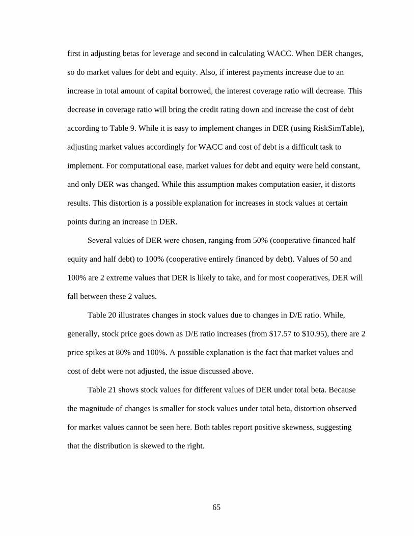
65
first in adjusting betas for leverage and second in calculating WACC. When DER changes,
so do market values for debt and equity. Also, if interest payments increase due to an
increase in total amount of capital borrowed, the interest coverage ratio will decrease. This
decrease in coverage ratio will bring the credit rating down and increase the cost of debt
according to Table 9. While it is easy to implement changes in DER (using RiskSimTable),
adjusting market values accordingly for WACC and cost of debt is a difficult task to
implement. For computational ease, market values for debt and equity were held constant,
and only DER was changed. While this assumption makes computation easier, it distorts
results. This distortion is a possible explanation for increases in stock values at certain
points during an increase in DER.
Several values of DER were chosen, ranging from 50% (cooperative financed half
equity and half debt) to 100% (cooperative entirely financed by debt). Values of 50 and
100% are 2 extreme values that DER is likely to take, and for most cooperatives, DER will
fall between these 2 values.
Table 20 illustrates changes in stock values due to changes in D/E ratio. While,
generally, stock price goes down as D/E ratio increases (from $17.57 to $10.95), there are 2
price spikes at 80% and 100%. A possible explanation is the fact that market values and
cost of debt were not adjusted, the issue discussed above.
Table 21 shows stock values for different values of DER under total beta. Because
the magnitude of changes is smaller for stock values under total beta, distortion observed
for market values cannot be seen here. Both tables report positive skewness, suggesting
that the distribution is skewed to the right.
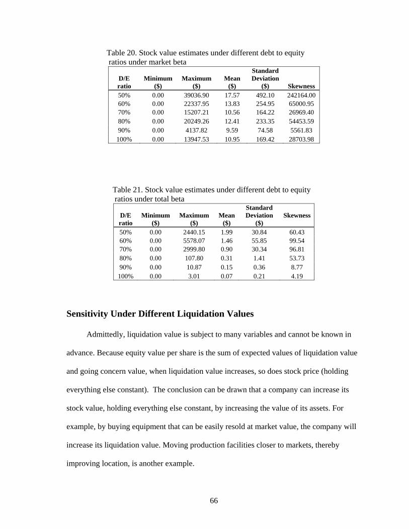
66
Table 20. Stock value estimates under different debt to equity ratios under market beta
D/E ratio
Minimum ($)
Maximum ($)
Mean ($)
Standard Deviation
($) Skewness 50% 0.00 39036.90 17.57 492.10 242164.00 60% 0.00 22337.95 13.83 254.95 65000.95 70% 0.00 15207.21 10.56 164.22 26969.40 80% 0.00 20249.26 12.41 233.35 54453.59 90% 0.00 4137.82 9.59 74.58 5561.83
100% 0.00 13947.53 10.95 169.42 28703.98
Table 21. Stock value estimates under different debt to equity ratios under total beta
D/E ratio
Minimum ($)
Maximum ($)
Mean ($)
Standard Deviation
($) Skewness
50% 0.00 2440.15 1.99 30.84 60.43 60% 0.00 5578.07 1.46 55.85 99.54 70% 0.00 2999.80 0.90 30.34 96.81 80% 0.00 107.80 0.31 1.41 53.73 90% 0.00 10.87 0.15 0.36 8.77
100% 0.00 3.01 0.07 0.21 4.19
Sensitivity Under Different Liquidation Values
Admittedly, liquidation value is subject to many variables and cannot be known in
advance. Because equity value per share is the sum of expected values of liquidation value
and going concern value, when liquidation value increases, so does stock price (holding
everything else constant). The conclusion can be drawn that a company can increase its
stock value, holding everything else constant, by increasing the value of its assets. For
example, by buying equipment that can be easily resold at market value, the company will
increase its liquidation value. Moving production facilities closer to markets, thereby
improving location, is another example.
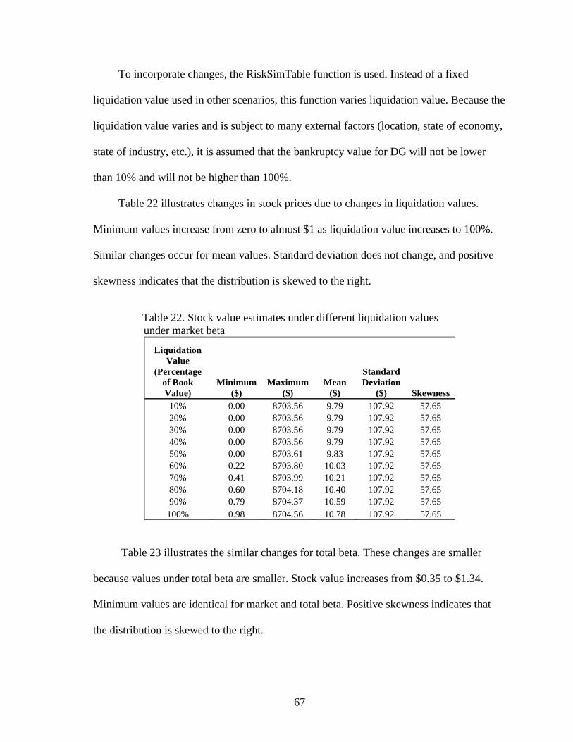
67
To incorporate changes, the RiskSimTable function is used. Instead of a fixed
liquidation value used in other scenarios, this function varies liquidation value. Because the
liquidation value varies and is subject to many external factors (location, state of economy,
state of industry, etc.), it is assumed that the bankruptcy value for DG will not be lower
than 10% and will not be higher than 100%.
Table 22 illustrates changes in stock prices due to changes in liquidation values.
Minimum values increase from zero to almost $1 as liquidation value increases to 100%.
Similar changes occur for mean values. Standard deviation does not change, and positive
skewness indicates that the distribution is skewed to the right.
Table 22. Stock value estimates under different liquidation values under market beta
Liquidation Value
(Percentage of Book Value)
Minimum ($)
Maximum ($)
Mean ($)
Standard Deviation
($) Skewness 10% 0.00 8703.56 9.79 107.92 57.65 20% 0.00 8703.56 9.79 107.92 57.65 30% 0.00 8703.56 9.79 107.92 57.65 40% 0.00 8703.56 9.79 107.92 57.65 50% 0.00 8703.61 9.83 107.92 57.65 60% 0.22 8703.80 10.03 107.92 57.65 70% 0.41 8703.99 10.21 107.92 57.65 80% 0.60 8704.18 10.40 107.92 57.65 90% 0.79 8704.37 10.59 107.92 57.65
100% 0.98 8704.56 10.78 107.92 57.65
Table 23 illustrates the similar changes for total beta. These changes are smaller
because values under total beta are smaller. Stock value increases from $0.35 to $1.34.
Minimum values are identical for market and total beta. Positive skewness indicates that
the distribution is skewed to the right.
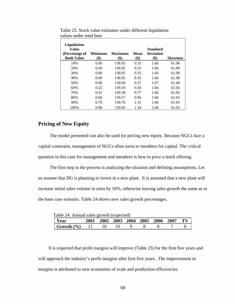
68
Table 23. Stock value estimates under different liquidation values under total beta
Liquidation Value
(Percentage of Book Value
Minimum ($)
Maximum ($)
Mean ($)
Standard Deviation
($) Skewness 10% 0.00 138.95 0.35 1.66 61.98 20% 0.00 138.95 0.35 1.66 61.98 30% 0.00 138.95 0.35 1.66 61.98 40% 0.00 138.95 0.35 1.66 61.98 50% 0.00 139.00 0.37 1.67 61.48 60% 0.22 139.19 0.58 1.66 61.93 70% 0.41 139.38 0.77 1.66 61.93 80% 0.60 139.57 0.96 1.66 61.93 90% 0.79 139.76 1.15 1.66 61.93
100% 0.98 139.95 1.34 1.66 61.93
Pricing of New Equity
The model presented can also be used for pricing new equity. Because NGCs face a
capital constraint, management of NGCs often turns to members for capital. The critical
question in this case for management and members is how to price a stock offering.
The first step in the process is analyzing the situation and defining assumptions. Let
us assume that DG is planning to invest in a new plant. It is assumed that a new plant will
increase initial sales volume in units by 50%, otherwise leaving sales growth the same as in
the base case scenario. Table 24 shows new sales growth percentages.
Table 24. Annual sales growth (expected)
Year 2001 2002 2003 2004 2005 2006 2007 TV Growth (%) 11 10 10 9 8 8 7 6
It is expected that profit margins will improve (Table 25) for the first five years and
will approach the industry’s profit margins after first five years. The improvement in
margins is attributed to new economies of scale and production efficiencies.
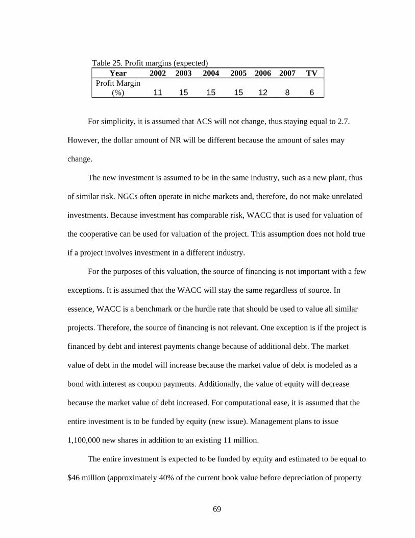
69
Table 25. Profit margins (expected)
Year 2002 2003 2004 2005 2006 2007 TV Profit Margin
(%) 11 15 15 15 12 8 6
For simplicity, it is assumed that ACS will not change, thus staying equal to 2.7.
However, the dollar amount of NR will be different because the amount of sales may
change.
The new investment is assumed to be in the same industry, such as a new plant, thus
of similar risk. NGCs often operate in niche markets and, therefore, do not make unrelated
investments. Because investment has comparable risk, WACC that is used for valuation of
the cooperative can be used for valuation of the project. This assumption does not hold true
if a project involves investment in a different industry.
For the purposes of this valuation, the source of financing is not important with a few
exceptions. It is assumed that the WACC will stay the same regardless of source. In
essence, WACC is a benchmark or the hurdle rate that should be used to value all similar
projects. Therefore, the source of financing is not relevant. One exception is if the project is
financed by debt and interest payments change because of additional debt. The market
value of debt in the model will increase because the market value of debt is modeled as a
bond with interest as coupon payments. Additionally, the value of equity will decrease
because the market value of debt increased. For computational ease, it is assumed that the
entire investment is to be funded by equity (new issue). Management plans to issue
1,100,000 new shares in addition to an existing 11 million.
The entire investment is expected to be funded by equity and estimated to be equal to
$46 million (approximately 40% of the current book value before depreciation of property
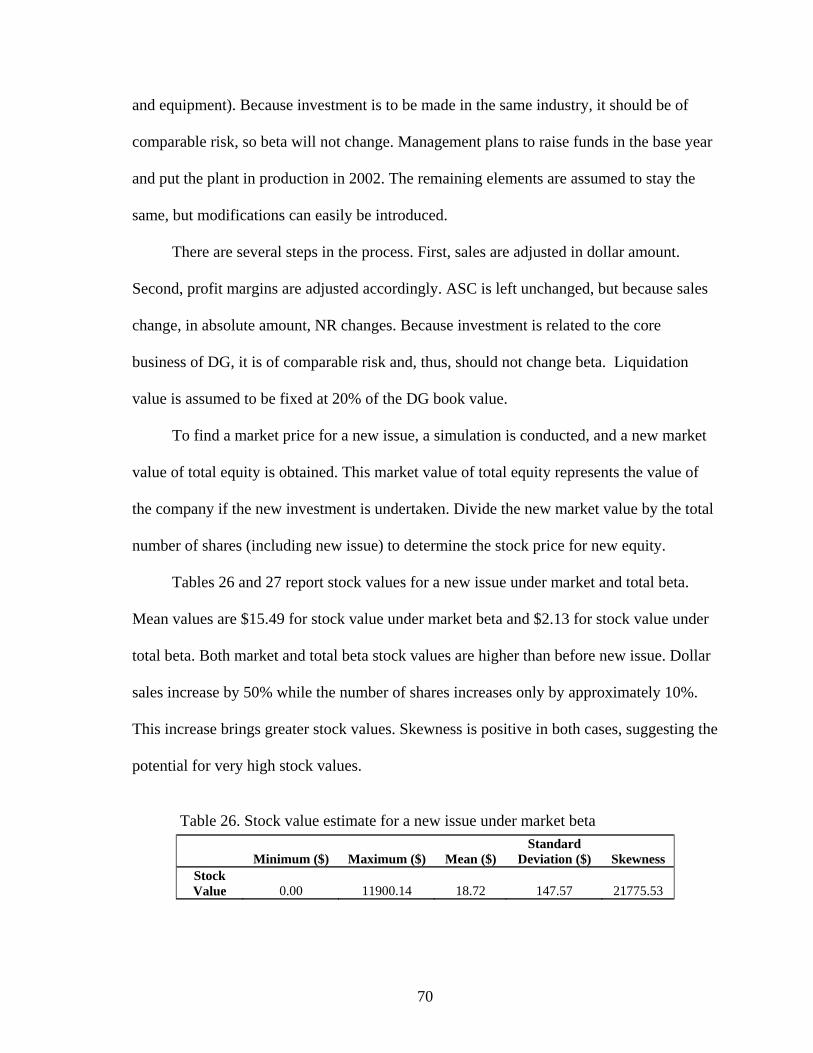
70
and equipment). Because investment is to be made in the same industry, it should be of
comparable risk, so beta will not change. Management plans to raise funds in the base year
and put the plant in production in 2002. The remaining elements are assumed to stay the
same, but modifications can easily be introduced.
There are several steps in the process. First, sales are adjusted in dollar amount.
Second, profit margins are adjusted accordingly. ASC is left unchanged, but because sales
change, in absolute amount, NR changes. Because investment is related to the core
business of DG, it is of comparable risk and, thus, should not change beta. Liquidation
value is assumed to be fixed at 20% of the DG book value.
To find a market price for a new issue, a simulation is conducted, and a new market
value of total equity is obtained. This market value of total equity represents the value of
the company if the new investment is undertaken. Divide the new market value by the total
number of shares (including new issue) to determine the stock price for new equity.
Tables 26 and 27 report stock values for a new issue under market and total beta.
Mean values are $15.49 for stock value under market beta and $2.13 for stock value under
total beta. Both market and total beta stock values are higher than before new issue. Dollar
sales increase by 50% while the number of shares increases only by approximately 10%.
This increase brings greater stock values. Skewness is positive in both cases, suggesting the
potential for very high stock values.
Table 26. Stock value estimate for a new issue under market beta
Minimum ($) Maximum ($) Mean ($)
Standard Deviation ($)
Skewness
Stock Value 0.00 11900.14 18.72 147.57 21775.53

71
Table 27. Stock value estimate for a new issue under total beta
Minimum ($) Maximum ($) Mean ($)
Standard Deviation ($)
Skewness
Stock Value 0.00 196.61 4.68 2.94 8.66

72
CHAPTER V. SUMMARY AND CONCLUSIONS
Introduction
This chapter provides an overview of the thesis, addresses limitations of the study,
indicates areas of possible improvement, and pinpoints areas for future research.
Summary of Thesis
The purpose of this study is to develop a model for valuation of an NGC’s equity.
An NGC is a cooperative engaged in agricultural value-added activities. It issues shares
that can be resold on a secondary market and carry a requirement to deliver processing
commodity.
NGCs were organized (in part) as a response to asset specificity. The asset specificity
problem occurs when a potential seller does not undertake a feasible investment (i.e.,
production of a specialized wheat variety) because of possible opportunistic behavior by a
future buyer. By becoming a member of the cooperative that will process this particular
commodity, a farmer becomes the buyer of the output it produces, effectively solving the
asset specificity problem. Besides addressing the problem, NGCs contribute to the local
economy, provide jobs, and enhance farmers’ incomes. All these benefits come with a price
of membership or equity investment into the cooperative. Membership to NGCs requires a
substantial initial investment, and NGCs rely heavily on members’ investments.
Importance of members’ investment explains why a liquid stock market, where price can
be easily determined, is essential to farmers, bankers, other investors, and NGC
management. However, there is limited trading of NGC stock due to a lack of eligible
commodity-producing members. Also, there are different tax obligations for NGCs and a
presence of delivery requirements for their stocks. Financial characteristics of the
73
cooperative, such as retained patronage, also contribute to the complexity of the problem.
At the present moment, there are no industry guidelines for valuation, and there is a need to
address this problem. A feasible pricing mechanism that provides these guidelines is
needed. This model aims to provide such a mechanism which approximates a fair value and
liquidity for the stock.
Results and Conclusions
This study addresses the problems described by developing a stock valuation model.
To accomplish this objective, a review of relevant literature is conducted. Also, a
spreadsheet simulation model, presented earlier, that utilizes the @Risk analytical tool is
developed. The model utilizes a discounted cash flows (DCF) approach to valuation. The
choice of this valuation tool is explained by the fact that little market data about NGCs
stock are available. Often, due to lack of market data, the best source of information is
financial statements about a company. Several different scenarios are conducted using the
model, and pricing of a new equity is illustrated. Stock values are considered for investors
at two extremes: stock price under market beta illustrates the stock value for the well-
diversified corporate investor, and stock price under total beta illustrates the stock price for
a non-diversified individual investor.
Stock value for the DG base case is $9.79 with a standard deviation of $107.92 and
positive skewness. Stock value under total beta is $0.35 with standard deviation of $1.68
and positive skewness.
The model indicates that stock value is positively correlated with profit margins. A
9% increase in profit margins (from 3% to 12%) boosts stock price under market beta by
almost $21 (from $3.53 to $24.17). Standard deviation increases from $53.85 to $215.93.
74
The increase under the total beta is smaller in dollar amount from $0.02 to $4.70, with
standard deviation increasing from $0.73 to $4.13. Skewness is positive in both cases.
Relationship between net reinvestments (NR) and stock price is examined by
changing the average sales to capital (ASC) ratio. As ASC increases (thus a decrease in
NR) from 2.5 to 3.4, stock price under market beta increases from $9.70 to $10.02. The
increase in standard deviation is only $0.03, and skewness is positive. The stock value total
beta increased from $0.29 to $0.53. The increase in standard deviation is the same as with
market beta, and skewness is positive as well.
Also, changes in debt to equity ratio (DER) are considered. It is shown that, albeit
with noise, stock price decreases as DER increases. As DER increases from 50% to 100%,
stock price falls from $17.57 to $10.95 under market beta and from $1.99 to $0.07 under
total beta.
Finally, the model is used to illustrate the pricing of new equity. A hypothetical plant
investment worth $40 million is introduced; as a result of this investment, stock value
under market beta increases to $15.49. The standard deviation is $147.53 with positive
skewness also indicated. The stock value under total beta is equal to $2.13 with a standard
deviation of $2.59 and positive skewness.
Possible Uses of the Model
The model presented in this thesis may contribute in solving liquidity problems and
easing financial constraints for NGCs. By suggesting a reasonable price, use of the model
aims to satisfy a buyer and a seller, and foster faster transactions. The reasonable price will
provide liquidity. Also, by promoting more trading activity, use of the model may help
bring more liquidity to the market.
75
By providing guidance for pricing equity, use of a model may benefit several groups
of people. Potential investors (potential members farmers) and potential sellers (current
members farmers) of NGC equity may be able to benefit from the model. Often, due to the
lack of consistent trading, sellers and buyers must evaluate such investment with old
information. The last transaction may have occurred months ago. During these months,
major changes in the cooperative or the environment it operates in can take place, changing
the value of the cooperative and equity dramatically. Profit margins may change, or
industry outlook may be different. With the model presented, potential and current
members will be able to incorporate these changes in the model and evaluate stock price.
NGC management may use NGC equity as collateral for obtaining loans. Knowing
the value of the stock is essential in this case. If the bank undervalues the equity, then the
NGC suffers from a higher cost of debt. Also, if a potential investor undervalues the equity,
a lower price will be offered, or a trade will not occur. NGC will suffer from a higher cost
of capital whether debt or equity. However, by employing this model, the bank (or other
investor) may more fully evaluate the stock’s value.
The given model also benefits NGC management by providing an expected stock
value at any given time. The model also illustrates what may happen to the stock value as a
result of a particular management decision or specific event beyond management control
(recession for example). By inputting necessary information, the model may enable
management to develop better strategy and to utilize resources more efficiently.
76
Summary
In conclusion, the importance of this study arises not from the final results but from
the methodology presented. The research presented shows guidelines and attempts to
develop a scientifically consistent way of appraising NGC stock values and should be
treated as such. The model can be useful by providing an expected stock value. By
providing timely information for the model (i.e., profit margins, sales, and sales growth),
an investor and management may get an approximation for the stock with current
information being incorporated in the stock value.
Limitations of the Research
There are several limitations of the research presented. By addressing these
limitations, the model can be improved further. One of the limitations of the current
research arises from its assumptions. The model uses industry accounting ratios that may
be different for the specific cooperative. One of the main differences between an investor
oriented firm (IOF) and a cooperative is that an IOF aims to maximize shareholder value.
While investors invest in an IOF to maximize return on their investment, members join a
cooperative to utilize its services. Because members of the cooperative are its suppliers as
well, a cooperative may accept lower profit margins if members want the cooperative to
pay higher prices for their inputs. Industry ratios are derived from IOF companies while
ratios for the cooperative may differ. The difference in profit margins can potentially create
problems for the valuation model (i.e., unrealistic profit margins).
Because beta for DG is not available, the model utilizes a proxy. While being
reasonably close, the beta may still differ in value. Because beta is an important input for
WACC, different values of beta will change WACC.
77
Liquidity discount in the model is assumed to be constant. In Chapter III, it is
mentioned that liquidity discount varies as the level of sales changes and as the company’s
assets become more/less liquid. The fact that liquidity discount does not change during
simulations may distort stock value.
While it is assumed that sales growth rate and risk-free rate follow normal
probability distribution, the potential problem arises if sales and/or risk-free rate do not
follow a normal probability distribution. Also, covariance between sales growth rate and
risk-free rate may change over time, instead of being constant. These issues may also
distort stock values.
The model utilizes bankruptcy probabilities. While it is assumed that probabilities
are the same across industries, it may not be necessarily true. Some industries are growing;
others are in decline. Some industries may be going through restructuring, consolidation
phases. The probability of an agricultural company going bankrupt may be different from
the bankruptcy probability for a communication company.
Future Research Areas
This section proposes possible solutions to the limitations of the research. These
solutions may improve the model and make results more precise for the cooperatives.
To address the ratio limitation, a systematic way of adjusting ratios should be
developed. Alternatively, if available, ratios for the cooperatives (estimated based on
specific industry cooperatives) should be used.
Beta for DG should be estimated. Traditionally, beta is estimated by running
regression between a market index (i.e., S&P) and stock price. Because stock price is not
available, Damodaran (2001) suggests the use of earnings instead of stock price.
78
To make the liquidity discount more responsive to the change in sales, correlation
between liquidity discounts and sales should be present in the model. Thus, correlation
should be estimated and incorporated in the model.
Distributions for risk-free rate and sales should be estimated. These results should be
incorporated in the model. Also, covariance between sales and risk-free rate should be
estimated on a regular basis. If covariance changes, the new covariance value should be
incorporated in the model.
Probability of the company going bankrupt in various industries should be estimated.
As it is mentioned, bankruptcy probabilities may differ widely among various industries.
Use of respective probabilities for the respective industries will improve the model and
enhance results.
Also, because the model utilizes @Risk, the model is subject to the limitation of the
software. Replication of the model in other simulation programs may improve the results
and illustrate new applications of the model.
Finally, while the model relies on modern financial valuation theory, more research
is needed to understand a farmer’s stock valuation process. A farmer’s approach to
valuation may be different from what financial theory suggests. As part of the research,
farmers’ perceptions should be surveyed and analyzed, and incorporated into the model if
possible.
79
REFERENCES
Altman, E. 1971. Corporate Bankruptcy in America. Heath Lexington Books, Lexington, Kentucky.
Amihud, Y., and H. Mendelson 1991. “Liquidity, Asset Prices, and Financial Policy.”
Financial Analyst Journal, Volume 47, Number 3, pp 56-66. Bangsund, D., and F. Leistritz, 1998. “Economic Contribution of the Sugarbeet Industry to
the Economy of North Dakota and Minnesota.” Department of Agricultural Economics, North Dakota State University. Fargo, Agricultural Economics Report 395.
Booth, L. 1999. “Estimating the Equity Risk Premium and Equity Costs, New Ways of
Looking at Old Data.” The Bank of America Journal of Applied Corporate Finance, Volume 12, Number 1, pp 100-112.
Chaddad, F., and M. Cook, 2002. “Testing for the Presence of Financial Constraints in U.S.
Agricultural Cooperatives.” Department of Agricultural Economics, University of Missouri. Columbia.
Cobia, D. W. 1989. Cooperatives in Agriculture. Prentice Hall, Englewood Cliffs, New
Jersey. Damodaran, A. 1999, “Estimating Risk-free Rates.” Working Paper. Stern School of
Business, New York. Damodaran, A. 2000. “The Dark Side of Valuation: Firms with No Earnings, No History
and No Comparables. Can Amazon.com Be Valued?” Working Paper. Stern School of Business, New York.
Damodaran, A. 2001, The Dark Side of Valuation: Valuing Old Tech, New Tech and New
Economy Companies, Prentice Hall, New York. Damodaran, A. 2002a, “Dealing with Distress in Valuation.” Working Paper. Stern School
of Business, New York. Damodaran, A. 2002b. Investment Valuation, 2nd Edition, John Wiley & Sons, New York. Fulton, M. 2001. “New Generation Co-operative Development in Canada.” Centre for the
Study of Co-operatives. University of Saskatchewan, Saskatoon, Saskatchewan, Canada.
Hitt, M., P. Clifford, R. Nixon, and K. Coyne, 1999. Dynamic Strategic Resources:
Development, Diffusion and Integration. John Wiley & Sons, New York.
80
Jensen, M. 1986. “Agency Cost of Free Cash Flow, Corporate Finance, and Takeovers.” The American Economic Review. Volume 76, Issue 2, pp 323-329.
Kaufold, I. 1997. “Two DCF Approaches and Valuing Companies Under Alternative
Financing Strategies (and How to Choose between Them).” The Bank of America Journal of Applied Corporate Finance,Volume 10, Number 1, pp 45-67.
Kraenzle, C., and R. Richardson, C. Adams, K. DeVille, and J. Penn. 1999. “Farmer
Cooperative Statistics”. United States Department of Agriculture Rural Business–Cooperative Service RBS Service Report 59, Washington, DC.
Leistritz, F., D. Bangsund, and J. Leitch, 1994. “Economic Impact of the Northern Corn
Processors’ Cooperative Proposed Corn Wet Milling Facility” Department of Agricultural Economics, North Dakota State University, Fargo. Agricultural Economics Report 94007.
Levy, H., and M. Sarnat, 1982. "Bankruptcy Risk and the Choice of Financial Structure."
Capital Investment and Financial Decisions, 2nd Edition. Prentice Hall International, Englewood Cliffs, New Jersey.
Mann, S., and N. Sicherman, 1991. “The Agency Cost of Free Cash Flow: Acquisition
Activity and Equity Issues.” The Journal of Business, Volume 64, Issue 2, pp 165-187. Moller, L., A. Featherstone, and D. Barton, 1996. “Sources of Financial Stress in
Agricultural Cooperatives” Journal of Cooperatives, Volume 11, pp 39-50. Moore, C., and J. Noel, 1995. “Valuation of Transferable Delivery Rights for Marketing
Cooperatives.” Journal of Cooperatives, Volume 10, pp 1-17. Olson, F. 2002. Personal Communication. Pates, M. 2002. “North Dakota Farmers to Vote on Status of Food Processing
Cooperative.” Tribune Business News. January, Washington. Pederson, G. 1998. “Cost of Capital for Agricultural Cooperatives.” University of
Minnesota-Twin Cities. Rural Business Services Report 163. Pettit, J. 1999. “Corporate Capital Costs: A practitioner’s guide.” The Bank of America
Journal of Applied Corporate Finance, Volume 12, Number 1, pp 113-120. Porter, M. 1980. Competitive Strategy. The Free Press, New York. Robak, E., and L. Hall, 2001. “Bringing Sanity to Marketability Discounts; A New Data
Source” Valuation Strategies.
81
Rose, P., and G. Gary, 1984. “Predicting Corporate Bankruptcy: An Analytical and Empirical Evaluation.” Review of Business and Economic Research. Volume 19, Number 2, pp 46-74.
Ross, S., R. Westerfield, and J., Jaffe, 1996. Corporate Finance. 4th Edition. Irwin,
Chicago. Rural Cooperatives, 2002. “Dakota Growers Pasta Eyes Conversion to C-corp.” Rural
Cooperatives, Volume 69, Issue 3, pp 32-34. Silber, W. 1991. “Discounts on Restricted Stock: The Impact of Illiquidity on Stock.” The
Financial Analysts Journal, Volume 47, pp 60-64. Skadberg, K. 1985. “Credit Scoring: Determining Bankruptcy in the Oilfield Service and
Equipment Industry” Paper, Department of Business Administration and Economics, North Dakota State University, Fargo.
Sporleder, T., and M. Bailey, 2001. “Using Real Options to Evaluate Producer Investment
in New Generation Cooperatives” Department of Agricultural, Environmental and Development Economics, The Ohio State University, Columbus.
Stefanson B., and M. Fulton, 1997 “New Generation Co-operatives: Responding to
Changes in Agriculture.” Centre for the Study of Cooperatives. University of Saskatchewan, Saskatoon, Saskatchewan, Canada.
Stefanson, B., M. Fulton, and A. Harris, 1995. “New Generation Cooperatives: Rebuilding
rural Economies.” Center for Study of Co-operatives. University of Saskatchewan, Saskatoon, Saskatchewan, Canada.