Equity Fund Ownership and

the Cross-Regional Diversification of Household Risk

Sascha O. Becker

Mathias Hoffmann

Stirling Economics Discussion Paper 2008-25

November 2008

Online at http://www.economics.stir.ac.uk

Equity Fund Ownership and the Cross-Regional

Diversification of Household Risk∗

Sascha O. Becker†

U Stirling, ifo, CESifo, and IZA

Mathias Hoffmann‡

University of Zurich and CESifo

November 21, 2008

Abstract

We explore the link between portfolio home bias and consumption risk sharing amongItalian regions using aggregated household level information on consumption, incomeand portfolio holdings. We propose to use data on equity fund ownership to proxy for re-gional home bias: equity funds are typically diversified at the national or internationallevel and will therefore provide interregional diversification. In assessing the impactof equity fund ownership on interregional risk sharing we distinguish between two di-mensions: variation in the share of equity funds in fund-holder’s wealth (the intensivemargin) and variation in the fraction of households that hold funds (the extensive mar-gin). We find that equity fund ownership is an important determinant of interregionalrisk sharing. First, diversification incentives qualitatively line up with actually observedportfolio choices: fund holders in regions where households are particularly exposed toregion-specific labor income risk hold a larger fraction of their wealth in (out-of-region)funds. Secondly, for a region as a whole, risk sharing increases in both the intensive andthe extensive margins of diversification and the two margins reinforce each other. Themarginal effect of wider equity fund participation seems particularly strong, suggestingthat policies aimed at increasing equity market participation could help foster betterinterregional risk sharing.

Keywords: consumption risk sharing, regional home bias, Survey of

Household Income and Wealth, labor income risk, portfolio choice, stock

market participation.

JEL codes: F36, F37, G1

∗We have received substantive comments during presentations at the CESifo Area Conference on Macro,Money and International Finance and at the University of Zurich. Discussions with Michel Beine and BentSørensen were very fruitful.

†Department of Economics, University of Stirling, Stirling, FK9 4LA, United Kingdom. E-Mail:sascha.becker@stir.ac.uk

‡University of Zurich, Institute for Empirical Research in Economics, Chair of International Trade andFinance, Zuerichbergstasse 14, CH-8032 Zurich. E-Mail: mathias.hoffmann@iew.uzh.ch

1

1 Introduction

Risk sharing between households, regions and nations has been the focus of an important

and continually growing literature over the last decade.1 Still, little is known to date about

the link between portfolio structure and consumption risk sharing at the regional level. In

this paper, we ask two questions. First, how do region-specific risks affect regional home

bias in household portfolios? And, secondly, how does household portfolio diversification

affect interregional risk sharing? By attempting to get at these issues, we hope to help close

an important gap, as we see it, between the macroeconomic literature on interregional risk

sharing and the literature on risk sharing and portfolio choice at the household level.

Our contribution is twofold: First, our regional evidence on the link between portfolio

structure and risk sharing complements existing international evidence in an important way.

In any attempt to gauge the impact of financial globalization on international risk sharing,

regional evidence serves as a natural empirical benchmark. Such a comparison was, however,

so far not possible with respect to international portfolio choice because regional evidence

on the link between portfolio structure and risk sharing virtually did not exist. We provide

such evidence here. Our results therefore provide a new perspective on the portfolio home

bias puzzle.

Our second contribution is to draw attention to the distinction between what we call

the two margins of diversification: increased participation in interregional asset markets

improves diversification along the extensive margin, whereas we refer to an increase in the

share of wealth held in out-of-region assets as improved diversification along the intensive

margin. The potential importance of this distinction has, to our reading, not been acknowl-

edged in the extant literature. In order to make the distinction between the two margins

empirically, we aggregate household level information about consumption, income and port-

folios to the regional level. Specifically, we make use of the Survey of Household Income

1Household level analyses start with Mace (1991) and Cochrane (1991) and Townsend (1994). Asdrubali,Sørensen and Yosha (1996), Hess and Shin (2000), and von Hagen (2000) are prominent examples of papersthat have studied the extent of risk sharing between regions. Sørensen and Yosha (1998), van Wincoop(1999) and Becker and Hoffmann (2006) have looked at risk sharing between countries.

2

and Wealth by the Banca d’Italia (SHIW). The SHIW combines detailed information on

household income and consumption patterns with data on the household’s portfolio of real

and financial assets for the years 1987 to 2004, making it particularly suited for our pur-

poses here. Household level data sets do, however, not generally contain direct information

about the cross-regional allocation of household assets and the SHIW is no exception to this

rule. The key innovation we propose to overcome this obstacle is to proxy for out-of-region

equity ownership through household level information about ownership of equity mutual

fund shares. The rationale for doing so is that equity funds are generally managed at a

national or even international level, so that through ownership of mutual fund shares the

household effectively achieves interregional diversification.

Our setup allows us to tackle the two questions we asked in the first paragraph. In

our answer to the first question, our point of departure is an observation from standard

portfolio theory: ceteris paribus, a household’s incentive to invest into out-of-region assets

rises in the its exposure to local (i.e. region-specific) economic conditions.2 We find this

prediction broadly fulfilled: regions with more strongly idiosyncratic GDP fluctuations hold

a larger share of their wealth in equity funds. While there is evidence that both margins

contribute to this finding, the effect of higher participation is insignificant. But households

that already do own equity funds seem to hold more of them in regions where they are more

exposed.

So, do more diversified regions share more risk overall? Our answer to this second

question is a qualified yes. We find that consumption risk sharing with the rest of the country

is better in regions in which more households participate in funds and where households hold

a relatively large fraction of their wealth in such instruments. The interaction between the

extensive and intensive margins of diversification plays a key role: the effects of higher fund

holdings on aggregate risk sharing are much stronger when fund ownership is widespread

in the population. Over our sample period, 1987-2004, increasing the participation rate by

one percentage point would have led to an about 2 percentage point increase in aggregate

2See e.g. Lucas and Heaton (2000, Econ J.) on the role of labor income risk for portfolio choice.

3

risk sharing. Conversely, the effect of inducing households to allocate a larger fraction of

their wealth to funds is much smaller. We find the intensive margin to be of significance

mainly during the bull market of the late 1990s, when unprecedentedly high participation

rates and high stock market valuations allowed many households to decouple consumption

from region-specific income shocks.

These findings suggest that stock market and in particular, equity fund participation, is

strongly associated with interregional diversification and that policies aimed at increasing

participation rates could possibly be highly effective in improving the nationwide pooling

of household level risks.

Our results also add important regional evidence to a recent literature in macroeco-

nomics and international finance that documents that portfolio diversification and con-

sumption risk sharing go hand in hand at the international level. Sørensen, Yosha, Wu and

Zu (2007) show that countries with larger international asset positions have larger cross-

border capital income flows and share more risk. Sørensen et al. therefore argue that the

equity home bias puzzle and the lack of international consumption risk sharing are twin

puzzles separated at birth. Our analysis here shows not only shows that this logic carries

over to the regional and even to the household level. It also points at the importance

of distinguishing between the two margins of diversification for understanding the impact

of financial globalization on risk sharing. To our knowledge, the role of participation in

financial markets for risk sharing has not been systematically explored.

The remainder of this paper is structured as follows. We describe our data and empir-

ical implementation in detail in the next section. Section three provides first descriptive

statistics on the characteristics of fund-owning and non-fund-owning households. Section

four presents our main results. We first explore a simple proposition: basic portfolio the-

ory would suggest that, ceteris paribus, a household’s incentive to invest into out-of-region

assets rises in the correlation of its labor income with region-specific economic conditions.

We show that this is indeed the case: regions where households are more strongly exposed

to region-specific risk have more fund owners and these fund owners invest a larger fraction

4

of their wealth into mutual funds. We then go on to investigate whether, in turn, regions

with lower ’home’ bias achieve better risk sharing. Section five summarizes and concludes.

2 Data and Empirical Implementation

2.1 The Survey of Household Income and Wealth (SHIW)

Our empirical analysis draws on a large-scale, public-use micro data set. The Italian Survey

of Household Income and Wealth (SHIW) gathers information on household income, con-

sumption and wealth, which makes it particularly well suited for our purposes. The SHIW

is collected by the Bank of Italy, is available from 1977 onwards and has been run on a

yearly basis until 1987 (with the exception of 1985) and every other year since then (with

the exception of 1995-1998 with a 3-year gap between surveys). From 1987 onwards, the

set of questions asked to respondents stabilized, allowing for consistent analyses over longer

time horizons. We concentrate our analysis on the period 1987-2004, thus covering nearly

two decades. The sample size is about 8,000 households per survey. Apart from a small

fraction of panel households,3 the SHIW consists of repeated cross-sections. This, however,

is not a problem for our analysis here, since we are interested in regional aggregates to

understand risk sharing patterns.

We restrict our sample to households where the household head is between 26 and 62

years of age. This excludes young household and pensioners without regular labor income.4

Since we analyze risk sharing, our aim is to define an income measure that properly

reflects households’ actual exposure to idiosyncratic risk as closely as possible. The literature

discusses various risk sharing channels including fiscal transfers and asset income. We

deliberately exclude these forms of income since they may already provide some form of

insurance. We therefore use the sum of net labor income from dependent employment,

net income from self-employment (entrepreneurial income), and rental income. This ’raw’

3The number of households that can be followed for 3 or more waves is too small to allow for an analysisof idiosyncratic household income and consumption risks over time.

4We experimented with different age ranges and results are robust when varying the minimum andmaximum age by some years.

5

income concept should be a reasonable reflection of the genuine sources of income risk that

households are exposed to. We summarize the exact construction of the data we use and

some key statistics in Table 1.

From a theoretical point of view, consumption is the flow of consumption “services”

resulting from both durable and non-durable goods. Whereas the former is not available,5

non-durable goods are thought of as delivering an immediate flow of services. Non-durable

consumption is thus our preferred consumption measure.

The SHIW also contains information on ownership of various asset classes, including

government bonds, individual stocks and equity funds. This constitutes a rich data source

for studying the impact of asset ownership on consumption smoothing. Section 3 discusses

in detail how we make use of these asset wealth data for our analysis. Again, we refer the

reader to Table 1 for a synopsis.

2.2 Constructing the regional data set

We form synthetic panel groups based on region of residence and fund-owner status to ob-

tain a panel of region-year observations. Not only does this allow us to obtain a regional

aggregate of all households, but it also allows us to distinguish between fund-holding and

non-fund-holding households at the regional level. Under the sampling plan of the SHIW,

each household is assigned a weight inversely proportional to its probability of inclusion in

the sample; the weights are supposed to align the structure of the sample with that of the

Italian population with respect to several known characteristics. We use these sampling

weights in the computation of region-level per capita variables. Our construction of syn-

thetic panel groups follows Attanasio and Davis (1996), who analyze repeated cross-sectional

data from the American Consumer Expenditure Survey (CEX) to study the effect of rela-

tive wage movements on the distribution of consumption. Whereas they form panel groups

by birth cohorts and education level of household head, our focus on regional risk-sharing

leads us to build region-level synthetic panel groups. The use of synthetic panel groups

5One would need access to item-by-item ownership of durable goods to derive consumption “services”under non-trivial assumptions.

6

constructed from household-level data has several advantages. First, whereas individual-

level studies potentially suffer from endogeneity of income (e.g. endogenous labor supply),

grouped data averages out individual-level idiosyncracies. Secondly, and differently from

regional accounts data, our household-level data contain information on fund-owning char-

acteristics that allow us to look at different household types instead of at (only) a single

representative household, as has virtually all of the earlier literature on regional risk sharing.

Our regional entities are the twenty administrative Italian regions: 1. Piemonte 2.

Valle d’Aosta 3. Lombardia 4. Trentino/Alto Adige 5, Veneto 6. Friuli/Venezia-Giulia

7. Liguria 8. Emilia-Romagna 9. Tuscany (Toscana) 10. Umbria 11. Marche 12. Lazio

13. Abruzzo 14. Molise 15. Campania 16. Puglia 17. Basilicata 18. Calabria 19. Sicily

(Sicilia) 20. Sardegna. However, in some regions and years, the SHIW has only very few

households owning stocks or mutual funds. In addition, due to the repeated cross-section

nature of the data set these households change over time, so that it becomes virtually

impossible to form a meaningful synthetic panel group of fund-owning households for some

of the smaller regions. In our empirical analysis, we take account of this by forming some

synthetic panel groups based on aggregates over several neighboring regions. Specifically,

we merge Val d’Aosta with Piemonte, Umbria with Tuscany, Molise with Puglia, Basilicata

and Sicily with Calabria and Sardegna with Lazio. While we experimented with alternative

groupings, we note that none of our results proved sensitive to this.

3 Measuring interregional diversification through mutual fund

ownership

Our main interest in this paper is to relate cross-regional risk sharing to household level

portfolio choice. Regional portfolios are the result of decisions at the household level. In

our analysis we therefore distinguish between households that own out-of-region productive

assets (i.e. equity) and households that do not. However, unlike at the international level,

data on regional portfolios do not exist. We therefore proxy ownership of out-of-region

productive assets with mutual fund ownership. The motivation for this choice is that most

7

mutual funds will hold a portfolio that is to the least nationally, if not internationally

diversified.

In this section, we first provide some descriptives on the characteristics of fund-owning

and non-fund owning households. We then suggest and discuss several measures of inter-

regional diversification that make use of fund-ownership information and that provide the

basis of our further analysis.

3.1 Mutual fund ownership: some descriptives

Table 1 gives some descriptive statistics about household owning mutual funds relative to

the average of the population.6 To compare the development of these characteristics over

time, we report numbers from the first (1987) and last (2004) year of our sample period

. The numbers suggest that owners of mutual fund shares have above average wealth

and high income. They are also more likely than the national average to be self-employed,

either in the free professions or as the owner-manager of their own or their family’s business.

However, our comparison over time clearly shows that fund holders were a more distinct

group back in 1987 than they are in 2004. Whereas in 1987, the fraction of fund-owners with

an upper-secondary schooling degree or more exceeded that of the population average by

far (75.2% vs. 39.2%), in 2004, that fraction actually falls in group of fund-owners whereas

in the population as a whole, there is a marked increase (74.8% vs. 50.1%). Similarly the

fraction of fund-owning households with self-employment income decreases from 47.3% to

30.8%. This reflects the trend for widening stock market participation and more widespread

fund holdings. Over our sample period, many relatively less affluent households seem to

have gained access to equity markets as is suggested in the marked decline in net disposable

income experienced by the average fund-owning household.

Table 2 provides a summary of asset portfolio characteristics for fund-holders and non-

fund-holders. Both groups have similar ratios of real assets to total net wealth. But the

6We consider as fund holders all households that report positive mutual fund holdings. We also exper-imented with various threshold levels, without any significant effect on any of the results reported in thepaper.

8

composition of the financial asset portfolio is quite different. Fund holders hold a much

larger fraction – roundabout a third in 1987 and almost two thirds in 2004 – of their

financial wealth in ’Other securities’. This asset category includes assets that are traded in

national capital markets such as the mutual fund shares that provide the basis for our cut

at the data here, but also foreign government securities, equity held outside of funds etc.

Clearly, ownership of mutual fund shares can only be an imperfect measure of the

interregional diversification of households. While our focus here is on household ownership

of out-of-region equity, households could also own other out-of-region assets. Bonds or

deposits may help countries to smooth consumption out of current income; households

could also own productive capital in other regions directly or through ownership of a private

business. Our data set does however not allow us to identify such out-of-region ownership

of equity or – for that matter – of bonds and deposits. Nor are we aware of any outside

data that would allow us to do so. Against the backdrop of these considerations, household

information on mutual fund ownership is, therefore, almost certainly a conservative proxy

of actual interregional equity cross-holdings.

Table 3 compares the standard deviations of growth rates in (’raw’) income, consump-

tion and net wealth across the two subgroups. Our measure of consumption is household

expenditure on non-durables. This measure excludes purchases of precious objects, cars,

furniture etc. Net wealth is measured as value of real assets plus financial assets minus

financial liabilities.

As is apparent, fund-holders have considerably more volatile income and consumption

flows and much more volatile wealth than their non-fund owning counterparts – a result

that suggests that fund owners face more idiosyncratic risk than the population average.

This finding is in line with the findings reported in Mankiw and Zeldes (1991) for stock

holders.

Table 4 shows cross-regional income and consumption correlations. For each Italian

region, column 1 provides the correlation of the consumption of fund owners residing in the

respective region with that of other fund owners in the rest of Italy. Column 2 gives the

9

analogous correlation for non-fund holders. In columns 3 and 4 we repeat the same exercise

for income. The cross-regional consumption correlation of fund owners is lower than that of

non-fund owners in 12 of 14 (aggregated) regions. For income this is true in 11 cases. The

average consumption correlation for fund owners is 0.096, that for other households 0.47.

For income, the respective correlations are 0.12 and 0.40.

The purely descriptive evidence in Tables 3 and 4 suggests that – as a group – fund

holders seem to face lots more idiosyncratic risk and that they achieve much less cross-

regional risk sharing than do non-fund holders. This ties in with the evidence in Tables 1

and 2 where we find that fund owners are more likely to be self-employed and hold a much

larger share of their wealth in business property. Heaton and Lucas (2000 J.Finance) have

prominently argued that proprietors constitute an important group of shareholders that is

also subject to non-insurable background risk. To the extent that fund-owners tend to be

proprietors, a higher share of fund owners may simply imply a lot more uninsurable region-

specific risk for them. In fact, Agronin (2003) provides evidence based on U.S. state level

data that regions with more small, proprietary businesses achieve less income insurance.

These findings may help rationalize the unconditional correlations we observe here.7

In this paper, we abstain from an attempt to explain why households own stocks or

mutual funds. Our approach is more modest: given that we observe that certain households

participate in stock markets – and in particular: mutual funds – we ask to what extent

cross-regional variation in the incentives to invest into out-of-region assets can explain

cross-regional variation in mutual fund ownership – both along the intensive as well as the

extensive margins. We then ask, to what extent the interaction between these two margins

can explain the relative success of a region as a whole in obtaining interregional consumption

risk sharing. We start by describing our diversification measures.

7Note that there is a version of the Backus, Kehoe and Kydland (1992) quantity puzzle in these householdgroup data: the average cross-regional consumption correlations of fund-owners is even lower than the averagecorrelation in their respective incomes.

10

3.2 Measures of interregional diversification: intensive and extensive mar-

gins

We now use the mutual fund holding characteristics discussed in the previous subsection to

obtain measures of interregional diversification (or, for that matter: home bias). Our data

set allows us to distinguish between two dimensions of interregional diversification: variation

across regions in the the fraction of the wealth held in mutual funds by households that

already own fund measures the intensive margin. Variation in mutual fund participation,

i.e. the fraction of all households in the region that own mutual funds at all measures the

extensive margin.8

We examine two measures of diversification along the intensive margin: our first mea-

sure puts the ratio of households’ mutual fund holdings to the value of their real assets.

This measure emphasizes the weight of fund owners out-of-region (i.e. mutual fund) assets

relative to what one might consider their local assets, notably owner occupied housing. We

call this measure MFW . As a second measure of diversification along the intensive margin,

we consider mutual fund holdings relative to fund owners’ labor income. We call this ratio

MFY . As a measure of diversification along the extensive margin we use the fraction of

households in a given region that own mutual funds, i.e. the mutual fund participation rate.

Table 5 gives an overview of the regional variation in our diversification measures. As is

apparent, there is a lot of dispersion in mutual fund ownership rates across regions. Fund

ownership is much more widespread in the northern regions such as Lombardia and Emilia-

Romagna, with 13 and 15 percent respectively, whereas in the southern regions such as

Calabria, Basilicata and Sicilia less than 2 percent of households hold mutual funds.

The share of wealth held in mutual funds, be it relative to local (i.e. housing) assets or

relative to income, still varies widely across regions., but somewhat less than does the fund

participation. Furthermore, the north-south divide, while present, is not quite as clear-cut

as it appears for the participation rates. Note that the two intensity measures MFW and

8We experimented with thresholds other than zero (strictly positive fund-holdings), e.g. more than2,000 EUR as minimum fund holdings to be classified as a fund-owning households, but results were largelyunaffected.

11

MFY are also very highly correlated across regions.

4 Results

4.1 Incentives for interregional diversification and household portfolios

In examining the link between interregional risk sharing and household portfolio character-

istics we take guidance from some simple principles of portfolio theory: the more exposed

households are to region-specific risks, the lower should ceteris paribus be the share of local

assets that the household would optimally want to hold in its portfolio. Hence, the share of

out-of-region assets should increase for households that are very exposed to region-specific

risk. Clearly, this is true only to the extent that expected return differentials between assets

in the home region and in the rest of the country are zero. Given that data limitations make

an empirical approximation of such expected return differentials between regions virtually

impossible and given that we want to focus on the role of portfolio choice for hedging con-

sumption risk, we make this assumption here. We measure incentives for the inter-regional

hedging of consumption risk using two different approaches:

In the first, we gauge how exposed households’ raw income is to region-specific GDP

shocks. This provides a measure of diversification incentives at the level of household types.

In the second, we gauge how strong diversification incentives are for the region as a whole

by asking to what extent its GDP fluctuations correlate with the national aggregate. We

then use a simple theoretical model to back out implied regional portfolio weights.

We implement the first approach by a regression of household income on regional GDP

growth

∆ykit = γki(∆gdpkt − ∆gdpt) + µki + vkit (1)

where ∆ykit is the growth rate of raw income for household-type i in region k and µki is a

region-specific fixed effect. As discussed in the previous section, we distinguish between two

household types – the average household in region k (i = all) and those households that

hold mutual funds (i = MF ).

12

We measure region specific economic conditions through the difference in GDP growth

rates between regions k and the national average, (∆gdpkt −∆gdpt). The coefficient γki can

then be interpreted as a measure of the sensitivity to local economic conditions.

The left panel of Figure 1 plots the estimates of γki for mutual fund holders (i = MF )

against the first of our intensive regional diversification measures, the ratio of mutual fund

holdings to local (real) assets (MFW ). As is apparent, there is a clear positive link between

the two variables and the regression coefficient seems highly significant. The figure highlights

the role of region-specific risk for diversification along the intensive margin:9 in regions,

where fund holders are particularly exposed to local economic conditions, they invest a

larger share of their wealth in mutual funds.

Interestingly, there is even a positive link between fund-holders degree of diversification

(the intensive margin) and average household exposure in the regions (see right panel of

Figure 1). This suggests that there is a strong correlation between the local exposures

of fund-owners and other households. The cross-sectional correlation between the γk for

fund-holders and non-fund-holders is bigger than 0.5. and highly significant. This does,

however, not imply that diversification along the extensive margin (participation rates) is

systematically higher in regions where people are strongly exposed to local economic shocks.

In the data, the link between mutual fund participation rates and exposure to local economic

conditions is insignificant. While explaining stock market participation is beyond the scope

of our analysis here, these result seem to deepen the puzzle of non-participation in equity

markets: given that diversification incentives are broadly the same for the two household

groups, it is surprising that they react so differently.

The coefficients γki are estimated from relatively short time series samples and are

therefore likely to be imprecise. The above cross-plots can therefore at best be suggestive

of a link between these variables. We attempt to solve this problem by parametrizing the

exposure coefficients γki as functions of mutual fund holdings directly. To this end, we

invert the conjectured linear relation between exposure and fund holdings underlying the

9To save space, we do not report the results for MFY graphically. The figure looks similar and the linkis is equally significant.

13

cross-plots above and write

γki = γi0 + γi′1 zik

where zik is a vector of region k household group i portfolio characteristics, γi0 is a group-

specific constant and γi′1 is a vector of coefficients. Specifically,we choose zikt to comprise

sample period averages of our intensive and extensive margin measures respectively as well

as their interactions. This parametrization for γik allows to write (1) as

∆ykit = γi0(∆gdpkt − ∆gdpt) + γi′1 zik(∆gdpkt − ∆gdpt) + µki + vkit (2)

which in turn puts us in a position to estimate γi0 and γi′1 from a panel regression. Again, µki

is the fixed effect. We note that, even though in this specification, γik varies as a function

of portfolio parameters, we do not want to to interpret this relation as a causal one. We

just want to ascertain statistically that actual diversification decisions are positively related

to diversification incentives as we measure them by household exposure to region-specific

economic conditions.

We provide results for regressions of the form (2) in the first two panels of Table 6. In

the first column of the table, zik consists of the intensive margin diversification measure, in

the second column we have the extensive margin. In the third column, zik includes both

measures and in the fourth column zik is the interaction between the two measures. We

find the intuition provided by the cross-plots largely confirmed. Panel I reports the results

for mutual-fund owning households. Higher fund holdings are clearly and significantly

associated with higher exposure. The extensive margin or the interaction between the two

margins are not significant. The same picture also emerges in panel II, where we consider

all households. It is variation along the intensive margin – i.e. higher fund-holdings by

households that already hold stocks – rather than variation in the incidence of fund-holding

households that is associated with higher exposure.

We further illustrate the link between diversification incentives and actual portfolio

choices using a second approach that imposes somewhat stronger theoretical restrictions.

14

Heathcote and Perri (2004) have suggested a model in which countries or regions can trade

claims that carry a dividend equal to a region’s per capita output. There is a friction in the

form of an iceberg cost on interregional dividend flows. Consumption in a region is then

a portfolio weighted average of home and rest of the country outputs (see also Artis and

Hoffmann (2008) and Crucini (1999) for similar models):

Ck = λGDP k + P k(1 − λ)(1 − τ)GDP (3)

where τ is the iceberg cost and P k is the price of a claim to region k output. Assuming that

utility is exponential and output log-normal with E(GDP kt ) = E(GDPt) = θ and variance

var(GDP kt ) = var(GDPt) = σ2 leads to the following optimal share in home asset holdings:

λ = min

{(1 − τ)2 − (1 − τ)ρ+ τθ

Aσ2

1 − 2(1 − τ)ρ+ (1 − τ)2, 1

}(4)

where A is the absolute risk aversion parameter. The min-operator ensures that countries

can not go short on foreign equity. We use this equation to calibrate optimal portfolio

shares for each region based on the correlation of its GDP growth rate with GDP in the

rest of the country 10, using a range of values for τ and the risk aversion parameter A.11

We then regress actual portfolio holdings on these calibrated portfolio weights. Panel III

of Table (6) provides the results of this exercise for τ = 0.05 and A = 1000.12 As is apparent,

there is significantly negative relation between the share of a region’s wealth held in mutual

funds and the optimal share of home assets held by the model. While the slope coefficient of

these regressions is not directly meaningful because the theoretical model is very stylized,

these results clearly line up with our earlier findings – actual patterns of interregional

10These data are taken from the CRENoS data base and are described in more detail in section 4.2 below

11The model assumes that the mean and variance of home and ’foreign’ output are identical. This as-sumption is a good approximation for Italian regional data.

12We experimented with a range of values for τ and A.The results were not sensitive to this choice,provided one chooses sufficiently high values of A. Values of A below 10 are are however implausible in thissetup because they lead to negative shares of home equity given the GDP correlations in the data. Anotherreason to choose rather high levels of risk aversion is that our analysis focuses on the hedging demand forout-of-region assets.

15

household diversification are consistent with theoretical diversification incentives: regions

that are more exposed to idiosyncratic risk seem to hold more out-of-region assets.

From the perspective of the region as whole, it is not clear a priori, along which margin

we should expect to see diversification to work when households are highly exposed to local

economic conditions. Higher diversification incentives could find their reflection both in

higher fund ownership rates and/or in more substantial holdings of out-of-region assets.

This impression is also confirmed by our second approach to measuring diversification in-

centives: if we regress participation rates or our intensive margin measures individually on

the calibrated values of λ (last three columns of panel III in Table 6), we always find a neg-

ative sign for the coefficient, but the link is not generally significant (though the evidence

in this case would point somewhat more strongly in the direction of the extensive margin).

Our findings here broadly suggest that diversification incentives, measured through cor-

relations of labor income with region-specific GDP fluctuations, seem to line up with actual

diversification behavior at the regional level. There is evidence that stronger diversifica-

tion incentives seem to lead to higher fund holdings of those households that already own

mutual funds. There is also a slightly higher propensity to participate in funds in regions

that are subject to more idiosyncratic shocks but the effect is not significant. This may

reflect liquidity constraints, costs of participation and other obstacles to equity ownership:

while diversification incentives may well be present for many households in the region, it

is plausible that mainly those households that hold equity anyway may be able to react to

them. It is beyond the scope of the paper to explain why households participate in equity

markets. While we would argue that non-participation clearly remains a puzzle also from

an interregional risk sharing perspective, the evidence from Table 6, panel III suggests that

regional participation patterns at least qualitatively line up the direction of diversification

incentives.

16

4.2 Does mutual fund ownership increase interregional risk sharing?

Our analysis so far has focused on how the structure of shocks faced by households in

different regions affects portfolio decisions. We now turn to asking what the effects of

portfolio diversification on interregional risk sharing may be. We first ask whether fund

owners as a group systematically share more consumption risk than do non-fund owners.

We then turn to the question whether regions as a whole share more risk if they have more

fund-owning households or if fund-owners hold a larger fraction of their wealth in mutual

funds.

4.2.1 Fund holders vs. non-fund holders

As our metric for risk sharing, we employ panel regressions of the form

∆cit(k) − ∆cit = βi(k)[∆ykit (k) − ∆yit

]+ µki + εiut (5)

Regressions of this kind have been proposed by Mace (1991) and Cochrane (1991) as tests

of the null of complete financial markets. We propose to interpret βi(k) as a measure of how

much of the idiosyncratic labor income risk of household group i in region k systematically

spills over into idiosyncratic consumption fluctuations. In particular, if βi(k) is unity, no

risk is shared, whereas if βi(k) = 0, all risk is shared. This interpretation of βi as a metric

for risk sharing was first popularized by Asdrubali, Sørensen and Yosha (1996).

We present the results obtained from regressions of this form for fund-holders and non-

fund-holders in Table 7. As is apparent, there is no major difference in the actual risk

sharing outcomes between owners of mutual funds and other households in the population.

Both groups insure between 40 and 50 percent of their idiosyncratic income shocks (the

respective βi for fund-holders is 0.57, and 0.60 for non-fund-holders). Interestingly, the

fraction of uninsured risk, βi, is virtually the same for both household groups, suggesting

that fund ownership per se – the ownership of out-of-region assets – does not necessarily

imply more or less interregional risk sharing. However, given the particular characteristics of

fund-owners as we documented them earlier, it is conceivable that an above average fraction

17

of fund owners’ idiosyncratic risk is non-diversifiable. The fact that, in spite of this, the same

fraction of all idiosyncratic risk is shared may suggest that fund owners could ultimately be

able diversify a larger portion of their diversifiable risk than the population as a whole. In

this respect our results here appear consistent with the view that fund ownership provides

interregional risk sharing ceteris paribus.

4.2.2 Impact on aggregate risk sharing

To explore the link between portfolio characteristics and interregional risk sharing on risk

sharing in the region aggregate, we again consider simple risk sharing regressions of the

form:

∆ct(k) − ∆ct = β(k)[∆ykt (k) − ∆yt

]+ µk + εut (6)

Note that this equation now applies to the regional aggregate and we therefore drop the

group index i in what follows. We then posit a linear relation between our (region-specific)

measure of risk sharing βu(k) and regional portfolio characteristics, so that

β(k) = β0 + β′zkt

where zkt is, again, a vector of region-specific characteristics. Plugging this relation into

(6), we obtain an equation with a set of interaction terms. Since we allow the vector of

characteristics to vary over time and across regions, the effect of the non-interacted zkt will

not be adequately captured by the region-specific fixed effect and we therefore also include

the non-interacted regional characteristics zkt into the regression which then becomes

∆ct(k) − ∆ct = β0 [∆yt(k) − ∆yt] + β′zkt [∆yt(k) − ∆yt] + δ′zkt + µk + εut (7)

The vector zikt contains our diversification measures, MFW and MFY , and the mutual

fund participation rate.

Table 8, column 1 reports the results for all households when no interaction terms are

considered. Around 55% of the region-specific income risk of the typical household remains

18

uninsured. Columns 2-8 report the results for the interaction term regressions (7). The

coefficients on the interaction terms are correctly signed throughout: more diversification,

be it along the intensive or extensive margin seems to lead to more risk sharing. This is true

for both of our intensive proxies, MPW and MPY . While MPY is highly significant, the

individual coefficients on MPW and on the participation measure appear only marginally

so. However, an F-test that they are jointly zero strongly rejects the null: when consid-

ered jointly, participation and higher household level portfolio diversification do tend to be

associated with more interregional risk sharing.

We expect the impact of diversification and participation on risk sharing to reinforce

each other: if all households own mutual funds the marginal effect of an increase in MPY

or MPW on aggregate risk sharing will be higher than if only very few households hold

funds. Conversely, we would expect that wider participation induces a larger increase in

aggregate risk sharing if average fund holdings are high than if they are low. To control for

such a potential non-linearity, we also include an interaction term between our intensive and

extensive (participation) measures. Columns 7 and 8 report on this exercise . The coefficient

on the interaction term is negative for both MFY and MFW : increasing diversification

along either margin increases the impact of the other margin on aggregate risk sharing.

To check the results in Tables 7 and 8 for robustness, we rerun our regressions including

a set of control variables into zikt that theory and earlier empirical work would suggest

could have an important bearing on interregional risk sharing: an indicator of a region’s

economic backwardness and remoteness (a Mezzogiorno dummy), the fraction of households

that report positive income from entrepreneurial activity. (Heaton and Lucas (2000a,b), and

Guiso et al. (1996)) and an index of regional specialization (Kalemli-Ozcan, Sørensen and

Yosha (2003)). The inclusion of these variables does not generally affect our results and none

of them was found to be individually significant. To capture the potential influence of other

omitted, slow moving variables such as financial development, we also experimented with

the inclusion of a linear trend. This somewhat affects the significance of the participation

measure, apparently due to some collinearity with the general increase in mutual fund

19

participation but leaves our other conclusions unaffected.

As an additional check, we obtain results similar to those in table 8 based on aggregate

regional data. So far, our findings were mainly based on household consumption and in-

come data that are aggregated up to the regional level. To make sure that our results from

these data are broadly representative, we we run our risk sharing regressions 7) , using the

micro-level information on fund holdings and participation rates, but now based on annual

growth rates of regional per capita consumption and GDP for the years 1987-2004 from

the CRENoS Regional Accounts data base Regio-IT 1970-2004 (Center for North South

Economic Research, http://www.crenos.it, see Paci and Saba, 1998). The setup of our

regression is otherwise analogous to the specification in the last column of table 8.13 The

results from this exercise are as follows: the coefficients on our diversification measures,

though numerically somewhat different, all have the same signs as in the regressions based

on household data. They are also all significant. This clearly strengthens our earlier con-

clusions: i) equity fund ownership seems to improve interregional risk sharing. ii) The

interaction between the intensive and extensive margins seems to matter for this result. We

explore next, how the contribution of these margins has varied over time.

4.2.3 Time variation in the margins of diversification

Our results on the interaction between extensive and intensive margins suggest that the

link between equity ownership and risk sharing has varied over our sample period: the

interaction between the two margins seems to matter in regression (7) which puts us in a

position to assess time variation in the marginal effect of diversification along the extensive

and intensive margins respectively. For the intensive margin measures, we have

∂βku∂ωkt

= β1 + β3PARTkt

13Since our diversification measures are observed only every second or sometimes even every third year(1995 and 1998), the interaction terms in the aggregate regressions are based on region-specific sampleaverages, so that we set zi

tk = zik for our regressions based on aggregate data.

20

as measure of the marginal effect of better diversification along the intensive margin and

∂βku∂PART kt

= β2 + β3ωkt

as marginal effect of higher participation, i.e. the extensive margin. Here, ωkt stands for

the time t share of mutual funds in fund-owners portfolio in region k, and PART kt is the

mutual fund participation rate in region k. In the remainder of this section, we report our

findings based on our first proxy, i.e. ωkt = MFW kt but note that all our results remain

virtually unchanged if we use MFY .

To compute the value of the marginal effects for the average region over our entire sample

period we use the time averages of the cross-sectional means of the respective variables:

PART =1T

∑t

PARTt =1TK

∑t

∑k

PART kt

ω =1T

∑t

ωt =1TK

∑t

∑k

ωkt

The first row of Table 9 provides the values of β1 + β3PART and β2 + β3ω along with

the p-value of an F-test that either of these effects was zero. We find that the marginal

effect along the intensive margin is −0.8 – a one percentage point increase in fund holdings

increases risk sharing by 0.8 percentage point, but this effect seems insignificant for the

sample period as a whole. Conversely, an increase in participation – the extensive margin –

increases aggregate risk sharing by more than 2 percentage points and this effect is highly

significant.

Both the mutual fund ownership rate as well as the valuation of shares and therefore the

share of wealth held in mutual funds have varied substantially over our sample period, so

that the numbers we just reported may mask considerable time-variation in the magnitude

and significance of the marginal effects. Figure 2 illustrates this point. The left panel

plots the cross-sectional mean participation rate PARTt and the one to the right the cross-

21

sectional mean holdings of mutual funds in real wealth, MFWt. Both reach a peak during

the stock market boom of the late 1990s. Therefore in the following rows of Table 9, we let

the intensive and extensive marginal effects for the average region vary over time by using

the cross-regional means PARTt and ωt = MFWt to compute them. For each year, this

part of the table reports the value of the variable driving the margin (i.e. PARTt for the

intensive and MFWt for the extensive margin), the value of the marginal effect and the

associated p− value.

The effect on aggregate risk sharing along the extensive margin is between 2 and 3

percentage points for most of the sample period and, with the exception for the year 1991,

also highly significant. Conversely, the effect of higher stock holdings, the intensive margin,

is subject to considerable time variation and insignificant in all but three years – 1998, 2000

and 2002 — when it also reaches 2-3 percentage points. These are the years of the technology

bull market and the immediate aftermath, when stock market participation reached a peak,

only to drop to pre-boom levels in the years till the end of our sample.

The results here support the view that fund ownership, on the margin, does provide

interregional risk sharing, even though our results above would suggest that fund holders

do not systematically share more risk across regional boundaries. But they also show

that at least in the early part of our sample, fund holders are a special group. Widening

mutual fund ownership to households with less specific characteristics, such as high levels

of non-diversifiable background risk is therefore likely to make a big impact on aggregate

risk sharing. This suggests that widening equity fund participation may be an important

avenue through which broader aggregate risk sharing can be brought about.

5 Summary and Conclusion

Our contribution in this paper has been twofold: first, we have explored the role of in-

terregional portfolio diversification for the patterns and extent of interregional risk sharing

between households. A number of current papers are exploring the link between risk sharing

and national portfolio structure in international data. It would seem that regional evidence

22

on the link between aggregate risk sharing and household portfolio choice should provide

an important benchmark for a better understanding of financial globalization. However,

virtually no evidence along these lines existed to date. Our results here help close this gap.

An important obstacle to region-level analyses of the link between risk sharing and

portfolio structure is that regional portfolio data do not exist. We suggest a solution to this

problem that is based on aggregating household level data from the Banca d’Italia Survey

of Household Income and Wealth (SHIW) from 1987-2004. One of our main innovations is

to use mutual equity fund ownership as a measure of out-of-region asset ownership : equity

funds tend to be managed at the national or even international level so that purchase of

mutual fund shares implicitly leads to interregional portfolio diversification.

Our second contribution is to draw attention to the interaction between what we call

the two margins of diversification for our understanding of aggregate risk sharing: varia-

tion in the share of mutual funds in fund-holders’ wealth captures the intensive margin of

diversification. Variation in the fraction of households that hold funds (i.e. in equity fund

participation rates) is the extensive margin. Based on this distinction, we uncover a number

of interesting links between household portfolio structure and interregional risk sharing.

First, fund owners living in regions where households are particularly exposed to region-

specific labor income risk hold a larger fraction of their wealth in equity funds. Equally,

in regions that are less correlated with the national average in terms of their GDP fluctu-

ations, a larger share of aggregate household wealth is held in equity funds and it seems

that both margins of diversification contribute to this regularity. These results suggest

that interregional diversification incentives qualitatively line up with actual diversification

patterns.

Secondly, we find no major difference in how much risk is shared by fund-owning and

non-fund-owning households, even though a larger fraction of the idiosyncratic income risk

faced by fund-holders is non-diversifiable (in line with the findings in e.g. Heaton and Lucas

(2000)). Our results therefore also appear consistent with the view that mutual fund owners

diversify away a larger fraction of their insurable risk than do non-owners.

23

Third, we document that regions with higher average mutual fund holdings and larger

mutual fund participation rates tend to achieve more risk sharing with the rest of the

country. Interestingly, the level and incidence of fund holdings have a mutually reinforcing

effect on risk sharing: the more widespread mutual fund holdings are, the larger is the

marginal effect on risk sharing of an increase of the fraction of fund-holders’ wealth invested

into mutual funds. These findings suggest that the link between regional portfolio structure

and risk sharing may vary in strength over time. Over our sample period, we estimate that

the marginal effects along both the intensive and extensive margins were highest during the

stock market boom of the late 1990s, when both asset valuations and participation rates

reached a peak.

Our results imply that policies aimed at increasing mutual fund ownership could have a

potentially important effect on interregional risk sharing. They also add a novel perspective

to an emerging literature in international finance that has recently started to investigate

the link between country portfolios and international consumption risk sharing. So far, this

literature has mostly focused on the impact of the recent decline in international portfolio

home bias on international consumption risk sharing. While our results here are not the

first to show that home bias is clearly not only an international phenomenon (for an early

contribution see Coval and Moskowitz (1999)), they may help shift the debate towards

the role of financial market participation – the extensive margin of diversification – for

understanding risk sharing at the aggregate level – be it between regions or countries.

24

References

Agronin, Eugene, “Risk-Sharing Across the United States, Proprietary Income, and the BusinessCycle,” mimeo, 2003.

Artis, Michael J. and Mathias Hoffmann, “Financial Globalization, International BusinessCycles, and Consumption Risk Sharing,” Scandinavian Journal of Economics, 2008, 110 (3),447–471.

Asdrubali, Pierfederico, Bent E. Sørensen, and Oved Yosha, “Channels of interstate risksharing: United States 1963-90,” Quarterly Journal of Economics, 1996, 111, 1081–1110.

Attanasio, Orazio and Steven J. Davis, “Relative Wage Movements and the Distribution ofConsumption,” Journal of Political Economy, December 1996, 104 (6), 1227–1262.

Backus, David K., Patrick J. Kehoe, and Finn E. Kydland, “International Real BusinessCycles,” Journal of Political Economy, 1992, 100 (4), 745–775.

Becker, Sascha O. and Mathias Hoffmann, “Intra-and International Risk-Sharing in the ShortRun and the Long Run,” European Economic Review, 2006, 50 (3), 777–806.

Cochrane, John H., “A Simple Test of Consumption Insurance,” Journal of Political Economy,1991, 99 (5), 957–976.

Coval, Joshua D. and Tobias J. Moskowitz, “Home Bias at Home: Local Equity Preference inDomestic Portfolios,” Journal of Finance, December 1999, 54 (6), 2045–2074.

Crucini, Mario J., “On International and National Dimensions of Risk Sharing,” The Review ofEconomics and Statistics, February 1999, 81 (1), 73–84.

Demyanik, Yuliya, Charlotte Ostergaard, and Bent E. Sørensen, “U.S. Banking Dereg-ulation, Small Businesses, and Interstate Insurance of Personal Income,” Journal of Finance,December 2007, 62 (6), 2763–2801.

Guiso, Luigi, Tullio Jappelli, and Daniele Terlizzese, “Income Risk, Borrowing Constraints,and Portfolio Choice,” The American Economic Review, March 1996, 86 (1), 158–172.

Heathcote, Jonathan and Fabrizio Perri, “Financial Globalization and Real Regionalization,”Journal of Economic Theory, 2004, 119, 207–243.

Heaton, John and Deborah Lucas, “Portfolio Choice and Asset Prices: The Importance ofEntrepreneurial Risk,” The Journal of Finance, June 2000, 55 (3), 1163–1198.

and , “Portfolio Choice in The Presence of Background Risk,” The Economic Journal, January2000, 110 (1), 1–26.

Hess, Gregory D. and Kwanho Shin, “Risk Sharing by Households Within and Across Regionsand Industries,” Journal of Monetary Economics, 2000, 45, 533–560.

25

Kalemli-Ozcan, Sebnem, Bent E. Sørensen, and Oved Yosha, “Risk Sharing and IndustrialSpecialization: Regional and International Evidence,” American Economic Review, June 2003, 93(3), 903–918.

Kraay, Aart, Norman Loayza, Luis Serven, and Jaume Ventura, “Country Portfolios,”Journal of the European Economic Association, June 2005, 3 (4), 914–945.

Lane, Philip D. and Gian Maria Milesi-Ferretti, “International Financial Integration,” IMFStaff Papers, 2003, 50 (Special Issue), 82–113.

Mace, Barbara J, “Full Insurance in the Presence of Aggregate Uncertainty,” Journal of PoliticalEconomy, October 1991, 99 (5), 928–956.

Mankiw, N. Gregory and Stephen P. Zeldes, “The consumption of stockholders and nonstock-holders,” Journal of Financial Economics, March 1991, 29 (1), 97–112.

Paci, Raffaele and Andrea Saba, “The empirics of regional economic growth in Italy 1951-93,”Rivista Internazionale di Scienze Economiche e Commerciali, 1998, 45, 515–542.

Sørensen, Bent E. and Oved Yosha, “International risk sharing and European Monetary Uni-fication,” Journal of International Economics, 1998, 45, 211–38.

and , “Producer Prices versus Consumer Prices in the Measurement of Risk Sharing,” AppliedEconomics Quarterly, 2007, 53 (1), 3–17.

, Yi-Tsung Wu, Oved Yosha, and Yu Zhu, “Home Bias and International Risk Sharing:Twin Puzzles Separated at Birth,” Journal of International Money and Finance, June 2007, 26(4), 587–605.

Townsend, Robert M., “Risk and Insurance in Village India,” Econometrica, May 1994, 62 (3),539–591.

van Wincoop, Eric, “How big are potential welfare gains from international risk sharing?,” Journalof International Economics, 1999, 47, 109–135.

von Hagen, Jurgen, “Fiscal Policy and Intranational Risk Sharing,” in Gregory D. Hess andEric van Wincoop, eds., Intranational Macroeconomics, Cambridge: Cambridge University Press,2000.

26

Table 1: Descriptive statistics: Full sample and fund-holder subsample

1987 2004Full Fund Full Fund

sample holders sample holders

Fund-holder (% of sample) 0.055 1 0.104 1(0.227) (0.305)

Age 45.205 46.508 46.96 48.224(9.729) (9.354) (9.41) (8.547)

Upper-secondary schooling (% of sample) 0.392 0.752 0.5 0.748(0.488) (0.432) (0.5) (0.435)

Proprietor (% of sample) 0.29 0.473 0.247 0.31(0.454) (0.5) (0.431) (0.463)

Transfer recipient (% of sample) 0.037 0.025 0.075 0.07(0.19) (0.157) (0.263) (0.255)

Net labor income (yl) 16.803 22.46 16.039 21.251(14.745) (22.244) (14.195) (17.765)

Pensions and other transfers (yt) 2.236 2.488 4.005 5.113(4.825) (5.393) (7.381) (9.156)

Pensions and pension arrears 2.073 2.361 3.683 4.763(4.7) (5.325) (7.229) (8.889)

Other transfers .163 .127 .322 .35(1.184) (1.006) (1.758) (1.815)

Net entrepreneurial income (ym) 7.901 19.752 6.257 9.458(17.945) (29.473) (24.876) (22.584)

Property income (yc) 4.455 13.787 5.92 11.051(8.13) (14.413) (8.003) (14.033)

Income from buildings (yca) 3.955 9.681 5.943 9.967(6.548) (11.482) (7.7) (13.593)

Income from financial assets (ycf) .5 4.106 -.023 1.084(3.73) (6.36) (2.154) (4.139)

Raw income (=yl+ym+yca) 28.659 51.892 28.238 40.676(22.374) (32.242) (29.276) (29.651)

Net disposable income excl. asset inc. (yraw+yt) 30.895 54.38 32.243 45.789(21.938) (31.715) (28.975) (28.631)

Net disposable income (yraw+yt+ycf) 31.396 58.486 32.22 46.873(23.07) (34.626) (29.21) (29.036)

Consumption (cn+cd) 24.602 41.534 23.993 32.39(15.618) (22.359) (13.713) (16.515)

Non-durable consumption (cn) 21.511 35.128 21.79 29.181(12.18) (18.361) (11.654) (14.48)

Durable consumption (cd) 3.091 6.406 2.203 3.209(6.492) (8.515) (5.414) (6.22)

Source: Italian Survey of Household Income and Wealth shiw, 1987-2004.Number of observations: 5,853 households in 1987, 4,776 households in 2004.All monetary variables are in 1,000s of current EUR.

27

Table 2: Descriptive statistics: Portfolio characteristics of fund-holders and non-fund-holders

1987 2004Fund non-Fund Fund non-Fund

holders holders holders holders

Real assets 322.844 112.651 350.501 184.699(464.666) (240.32) (540.451) (310.358)

Real estate (housing and land) 219.133 83.981 284.379 154.237(273.602) (141.266) (315.659) (223.869)

Businesses 87.756 24.039 57.685 25.776(326.615) (160.922) (343.269) (164.97)

Valuables 15.955 4.63 8.437 4.686(25.432) (13.162) (30.461) (12.818)

Financial assets 67.176 19.038 64.075 15.894(73.523) (36.643) (126.561) (50.421)

Deposits, CDs, repos, postal savings certificates 23.242 13.02 15.19 10.421(27.766) (21.722) (27.999) (29.495)

Government securities 21.145 4.777 5.248 1.757(32.936) (20.315) (21.342) (10.427)

Other securities (bonds, mutual funds, equity etc.) 22.789 1.241 43.637 3.715(33.904) (11.82) (108.457) (36.256)

Financial liabilities 4.451 3.031 11.192 8.246(14.993) (16.521) (35.571) (22.763)

Fin. liab. for purchase of real estate and other real assets 3.622 2.423 9.738 7.136(14.396) (16.278) (35.07) (22.407)

Other Financial Liabilities 0.829 0.608 1.454 1.11(2.799) (2.522) (4.72) (3.482)

Net wealth = Real assets + Financ. assets - Financ. liab. 385.569 128.658 403.383 192.347(497.159) (252.247) (569.263) (323.434)

Real net wealth = Real assets - Financ. liab on real estate 319.222 110.227 340.763 177.563(465.145) (238.695) (536.416) (305.045)

Source: Italian Survey of Household Income and Wealth shiw, 1987-2004.Number of observations: 5,853 households in 1987, 4,776 households in 2004.Net wealth = Real assets + Financ. assets - Financ. liab.Real net wealth = Real assets - Financ. liab on real estateAll monetary variables are in 1,000s of current EUR.

28

Table 3: Standard deviation of growth rates in consumption, income,and wealth

Fund-holders Non-fund-holdersNon-durable consumption 0.115 0.053

Durable consumption 0.249 0.204’Raw’ income 0.081 0.053Wealth 0.192 0.070

Source: Italian Survey of Household Income and Wealth shiw, 1987-2004.Standard-deviation computed over average growth rates of given variables in consecutive surveyyears, separately for fund-holders and non-fund-holders.For definition of variables, see main text and Table 1.

29

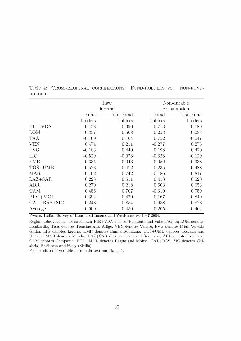
Table 4: Cross-regional correlations: Fund-holders vs. non-fund-holders

Raw Non-durableincome consumption

Fund non-Fund Fund non-Fundholders holders holders holders

PIE+VDA 0.158 0.396 0.713 0.780LOM -0.357 0.508 0.253 -0.033TAA -0.169 0.164 0.752 -0.047VEN 0.474 0.211 -0.277 0.273FVG -0.183 0.440 0.198 0.420LIG -0.529 -0.073 -0.323 -0.129EMR -0.335 0.043 -0.052 0.338TOS+UMB 0.523 0.472 0.235 0.488MAR 0.102 0.742 -0.186 0.817LAZ+SAR 0.228 0.511 0.418 0.520ABR 0.270 0.218 0.603 0.653CAM 0.455 0.707 -0.319 0.759PUG+MOL -0.394 0.470 0.167 0.840CAL+BAS+SIC -0.243 0.854 0.688 0.823Average 0.000 0.450 0.205 0.464

Source: Italian Survey of Household Income and Wealth shiw, 1987-2004.Region abbreviations are as follows: PIE+VDA denotes Piemonte and Valle d’Aosta; LOM denotesLombardia; TAA denotes Trentino-Alto Adige; VEN denotes Veneto; FVG denotes Friuli-VeneziaGiulia; LIG denotes Liguria; EMR denotes Emilia Romagna; TOS+UMB denotes Toscana andUmbria; MAR denotes Marche; LAZ+SAR denotes Lazio and Sardegna; ABR denotes Abruzzo;CAM denotes Campania; PUG+MOL denotes Puglia and Molise; CAL+BAS+SIC denotes Cal-abria, Basilicata and Sicily (Sicilia).For definition of variables, see main text and Table 1.

30

Table 5: Extensive and intensive margins of fund ownership

Region % Fund-holders MFW MFYPIE+VDA 0.096 0.099 0.642LOM 0.129 0.111 0.671TAA 0.079 0.059 0.433VEN 0.101 0.080 0.560FVG 0.104 0.075 0.591LIG 0.112 0.096 0.669EMR 0.155 0.076 0.624TOS+UMB 0.085 0.063 0.523MAR 0.086 0.064 0.593LAZ+SAR 0.035 0.062 0.449ABR 0.042 0.178 1.582CAM 0.016 0.050 0.285PUG+MOL 0.031 0.103 0.834CAL+BAS+SIC 0.016 0.062 0.443

Source: Italian Survey of Household Income and Wealth shiw, 1987-2004.Region abbreviations are as follows: PIE+VDA denotes Piemonte and Valle d’Aosta; LOM denotesLombardia; TAA denotes Trentino-Alto Adige; VEN denotes Veneto; FVG denotes Friuli-VeneziaGiulia; LIG denotes Liguria; EMR denotes Emilia Romagna; TOS+UMB denotes Toscana andUmbria; MAR denotes Marche; LAZ+SAR denotes Lazio and Sardegna; ABR denotes Abruzzo;CAM denotes Campania; PUG+MOL denotes Puglia and Molise; CAL+BAS+SIC denotes Cal-abria, Basilicata and Sicily (Sicilia).MFW is the ratio of funds over fund holder’s real assets (including housing).MFY is the ratio of funds over fund holder’s raw income.

31

Table 6: Interregional diversification patterns and diversification in-centives

Panel I: Fund-owners: diversification incentives(1) (2) (3) (4)

MFW 162.784 186.411(56.927)∗∗∗ (58.382)∗∗∗

Participation rate -30.119 -59.867(37.422) (37.125)

MFW * Participation rate 139.748(399.769)

Number of obs. 112 112 112 112R2 0.070 0.006 0.092 0.001

Panel II: Full sample: diversification incentives(1) (2) (3) (4)

MFW 45.906 50.965(19.951)∗∗ (20.615)∗∗

Participation rate -4.685 -12.818(12.983) (13.109)

MFW * Participation rate 91.991(138.168)

Number of obs. 112 112 112 112R2 0.053 0.008 0.062 0.011

Panel III: Diversification patterns a la Heathcote and Perri (2004)Total diversification Intensive and extensive marginsEquity fund-holdings Participation Equity fund-holdings

Dependent variable: over region-total rate over share-holderreal wealth income real wealth income

(1) (2) (3) (4) (5)

Optimal PF share λ -0.047 -0.229 -0.202 -0.095 -0.550(0.013)∗∗∗ (0.089)∗∗∗ (0.114)∗ (0.093) (0.485)

Number of obs. 14 14 14 14 14R2 0.502 0.359 0.208 0.079 0.097

Source: Italian Survey of Household Income and Wealth shiw, 1987-2004.Panels I and II show coefficients γi

1 from equation (2): ∆ykit = γi

0(∆gdpkt −∆gdpt) +γi′

1 zik(∆gdpkt −

∆gdpt) + µki + vkit

Panel III shows coefficients bx from the cross-sectional regression xk = const+ bxλk where λk is theoptimal share of home assets in region k’s portfolio and xk are the dependent variables given in thetable header.MFW is the ratio of funds over fund holder’s real assets (including housing).

32

Table 7: Unsmoothed component: Fund-holders vs non-fund-holders

Fund-holders Non-fund-holders(1) (2)

∆yut (k) .569 .596(.061)∗∗∗ (.060)∗∗∗

Obs. 112 112

Source: Italian Survey of Household Income and Wealth shiw, 1987-2004.Table shows βi(k) from equation (3) in the main text: ∆cit(k) − ∆cit = βi(k)

[∆yki

t (k)−∆yit

]+

µki + εiut.

βi(k) measures the fraction of income risk that is uninsured.

33

Tab

le8:

Unsm

oothed

component:

Full

sample

(1)

(2)

(3)

(4)

(5)

(6)

(7)

(8)

∆y

u t(k

)β0

0.5

42

0.6

84

0.7

71

0.7

15

0.8

18

0.8

75

0.5

95

0.5

44

(0.0

60)∗∗∗

(0.0

96)∗∗∗

(0.1

06)∗∗∗

(0.1

02)∗∗∗

(0.1

19)∗∗∗

(0.1

24)∗∗∗

(0.1

81)∗∗∗

(0.2

26)∗∗

Inte

nsi

ve

margin

:F

un

dh

old

ings

over

real

net

wea

lth

β1

-1.4

98

-1.2

24

1.9

81

(MFW

)(0

.870)∗

(0.8

71)

(2.0

82)

Fu

nd

hold

ings

over

raw

inco

me

β1

-0.3

93

-0.3

39

0.3

32

(MFY

)(0

.151)∗∗∗

(0.1

53)∗∗

(0.4

15)

Exte

nsi

ve

margin

:F

ract

ion

of

fun

d-h

old

ers

β2

-2.1

76

-1.9

63

-1.6

90

0.4

75

2.1

47

(1.0

29)∗∗

(1.0

36)∗

(1.0

38)

(1.8

01)

(2.3

46)

Inte

racti

ons:

Exte

nsi

ve

*in

ten

sive

marg

in1

β3

-34.7

37

(19.9

59)∗

Exte

nsi

ve

*in

ten

sive

marg

in2

β3

-7.4

26

(4.0

72)∗

p-v

alu

eof

F-s

tati

stic

of

join

tsi

gn

ifica

nce

0.0

408

0.0

109

of

main

effec

tsof

inte

nsi

ve

an

dex

ten

sive

marg

in

Ob

s.112

112

112

112

112

112

112

112

Sourc

e:

Italian

Su

rvey

of

Hou

seh

old

Inco

me

an

dW

ealt

hsh

iw,

1987-2

004.

Tab

lesh

ow

sβ

i(k

)fr

om

equ

ati

on

(3)

inth

em

ain

text:

∆ci t

(k)−

∆ci t

=β

i(k

)[ ∆y

ki

t(k

)−

∆y

i t

] +µ

ki

+εi u

t.

βi(k

)m

easu

res

the

un

smooth

edth

efr

act

ion

of

inco

me

risk

that

isu

nin

sure

d.

Colu

mns

(2)

thro

ugh

(4)

posi

tβ

i(k

)=β0

+β

i′z

ik tan

dm

easu

reh

ow

the

un

smooth

edco

mp

on

ent

isaff

ecte

dby

the

inte

nsi

ve

an

dex

ten

sive

marg

ins

of

fun

dh

old

ings.

34

Tab

le9:

Margin

al

effects:

Full

sample

inte

nsi

ve

marg

inex

ten

sive

marg

in%

fun

d-o

wner

sp

-valu

em

arg

.eff

ect

MF

Wp

-valu

em

arg

.eff

ect

(1)

(2)

(3)

(4)

(5)

(6)

1989-2

004

0.0

80

0.3

89

-0.8

00

0.0

87

0.0

21

-2.5

44

1989

0.0

27

0.5

18

1.0

46

0.0

99

0.0

13

-2.9

52

1991

0.0

29

0.5

38

0.9

73

0.0

64

0.1

06

-1.7

41

1993

0.0

52

0.8

78

0.1

90

0.0

92

0.0

16

-2.7

27

1995

0.0

51

0.8

75

0.1

94

0.0

77

0.0

38

-2.2

15

1998

0.1

14

0.0

42

-1.9

83

0.0

99

0.0

13

-2.9

47

2000

0.1

38

0.0

25

-2.8

27

0.1

13

0.0

10

-3.4

54

2002

0.1

33

0.0

26

-2.6

33

0.0

78

0.0

35

-2.2

49

2004

0.0

96

0.1

25

-1.3

59

0.0

73

0.0

51

-2.0

69

Sourc

e:

Italian

Su

rvey

of

Hou

seh

old

Inco

me

an

dW

ealt

hsh

iw,

1987-2

004.

Tab

lep

rovid

eses

tim

ate

sof

the

marg

inal

effec

tsof

div

ersi

fica

tion

alo

ng

the

inte

nsi

ve

an

dex

ten

sive

marg

inover

tim

e.T

he

inte

nsi

ve

marg

ineff

ect

isca

lcu

late

dasβ1

+β3∗

per

centa

ge

of

fun

d-h

old

ers

inyea

rt.

Th

eex

ten

sive

marg

inis

calc

ula

ted

asβ1

+β2∗MFW

inyea

rt.t=

1989,...2004.

Th

ees

tim

ate

sofβ1,β2

an

dβ3

are

from

Tab

le8.

Th

eco

lum

np

-valu

ep

rovid

esth

ep

rob

ab

ilit

yth

at

eith

erm

arg

inal

effec

tis

zero

.

35

Figure 1: Diversification incentives

Source: SHIW, 1987-2004, authors’ own calculations.On the y-axis: fund-holdings over real wealth for fund-holders in region i. On the x-axis: γki from the followingregression of household income (yraw from Table 1) on regional GDP growth: ∆yki

t = γki(∆gdpkt −∆gdpt) +

µki + vkit where k=fund-owning households (left panel) or k=all households (right panel).

Figure 2: Trends in share of fund-owners and in ratio of fund volumes overraw income

Source: SHIW, 1987-2004, authors’ own calculations.Both panels show Italy-wide averages.

36