Equilibrium Tuition, Applications, Admissions and

Enrollment in the College Market�

Chao Fuy

December 7, 2013

Abstract

I develop and estimate a structural equilibrium model of the college market. Students,

having heterogeneous abilities and preferences, make college application decisions, subject to

uncertainty and application costs. Colleges, observing only noisy measures of student ability,

choose tuition and admissions policies to compete for more able students. Tuition, applica-

tions, admissions and enrollment are joint outcomes from a subgame perfect Nash equilibrium.

I estimate the structural parameters of the model using data from the National Longitudinal

Survey of Youth 1997, via a three-step procedure to deal with potential multiple equilibria. In

counterfactual experiments, I use the model �rst to examine the extent to which college enroll-

ment can be increased by expanding the supply of colleges, and then to assess the importance

of various measures of student ability.

Keywords: College market, tuition, applications, admissions, enrollment, discrete choice, mar-

ket equilibrium, multiple equilibria, estimation

�I am immensely grateful to Antonio Merlo, Philipp Kircher, and especially to my main advisor Kenneth Wolpinfor invaluable guidance and support. I thank the editor and three anonymous referees for their suggestions, whichhave signi�cantly improved the paper. I thank Kenneth Burdett, Steven Durlauf, Aureo De Paula, Hanming Fang,Ken Hendricks, John Kennan, George Mailath, Guido Menzio, Andrew Postlewaite, Frank Schorfheide, Xiaoxia Shi,Alan Sorensen, Chris Taber, Petra Todd and Xi Weng for insightful comments and discussions. Comments fromparticipants of the NBER 2010 Summer Labor Studies, Search and Matching Workshop were also helpful. All errorsare mine.

yDepartment of Economics, University of Wisconsin, Madison, WI 53706, USA. Email: cfu@ssc.wisc.edu.

1

1 Introduction

Both the level of college enrollment and the composition of college students continue to be issues

of widespread scholarly interest as well as the source of much public policy debate. In this paper, I

develop and structurally estimate an equilibrium model of the college market. It provides insights

into the determination of the population of college enrollees and permits quantitative evaluation

of the e¤ects of counterfactual changes in the features of the college market. The model inter-

prets the allocation of students in the college market as an equilibrium outcome of a decentralized

matching problem involving the entire population of colleges and potential applicants. As a result,

counterfactuals that directly involve only a subset of the college or student population can produce

equilibrium e¤ects for all market participants. My paper thus provides a mechanism for assessing

the market equilibrium consequences of changes in government policies on higher education.

While the idea of modeling college matching as a market equilibrium problem is not new, this

paper makes advances relative to the current literature by simultaneously modeling three aspects

of the college market that are plausibly regarded as empirically important and incorporating them

into the empirical analysis. The three aspects are: 1) Application is costly to the student. Besides

application fees, a student has to spend time and e¤ort gathering and processing information and

preparing application materials. Moreover, she also incurs nontrivial psychic costs such as the

anxiety felt while waiting for admissions results. 2) Students di¤er in their abilities and preferences

for colleges.1 3) While trying to attract and select more able students, colleges can only observe

noisy measures of student ability, such as student test scores and essays. As a result, both sides of

the market face uncertainties: for the student, admissions are uncertain, which, together with the

cost of application, leads to a non-trivial portfolio problem: how many and which, if any, colleges

to apply to? For the college, the yield of each admission and the quality of a potential enrollee are

both uncertain. Colleges have to account for students�strategies in order to make inference about

student quality. Colleges�policies are also interdependent because students�application portfolios

and their enrollment depend on the policies of all colleges.

I model three stages of the market. First, colleges simultaneously announce their tuition. Second,

students make application decisions and colleges simultaneously choose their admissions policies.

Third, students make their enrollment decisions. My model incorporates tuition, applications, ad-

missions and enrollment as joint outcomes from a subgame perfect Nash equilibrium (SPNE). SPNE

in this model need not be unique. Multiplicity may arise from two sources: 1) multiple common self-

ful�lling expectations held by the student about admissions policies, and 2) the strategic interplay

among colleges.2

Building on Moro (2003), I estimate the model in three steps. The �rst two steps recover all the

1Throughout the paper, a student�s ability refers to her readiness for college, not her innate ability.2Models with multiple equilibria do not have a unique reduced form and this indeterminacy poses practical

estimation problems. In direct maximum likelihood estimation of such models, one should maximize the likelihoodnot only with respect to the structural parameters but also with respect to the types of equilibria that may havegenerated the data. The latter is a very complicated task and can make the estimation infeasible.

1

structural parameters involved in the application-admission subgame without having to impose any

equilibrium selection rule. In particular, each application-admission equilibrium can be uniquely

summarized by the set of probabilities of admission to each college for di¤erent types of students.

The �rst step, using simulated maximum likelihood, treats these probabilities as parameters and

estimates them along with fundamental student-side parameters in the student decision model,

thereby identifying the equilibrium that generated the data. The second step, based on a simulated

minimum distance estimation procedure, recovers the college-side parameters by imposing each

college�s optimal admissions policy. Step three recovers the remaining parameters by matching

colleges�optimal tuition with observed tuition levels.

To implement the empirical analysis, I use data from the National Longitudinal Survey of

Youth 1997 (NLSY97), which provides detailed information on student applications, admissions,

�nancial aid and enrollment. Some of my major �ndings are as follows: �rst, students not only

attach di¤erent values to the same college, but also rank various colleges and the non-college option

di¤erently. That is, there is not a single best college for all, nor is attending college better than the

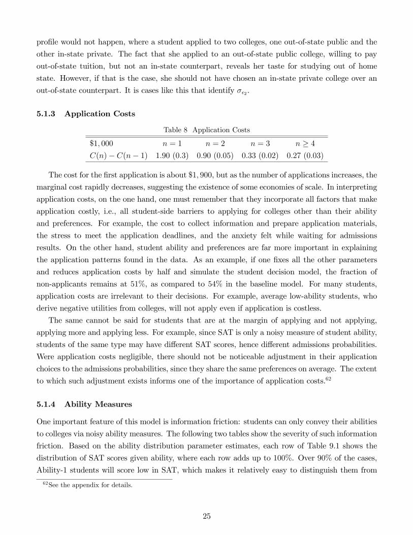
non-college option for all. My �rst counterfactual experiment �nds that increasing the supply of

colleges has very limited e¤ect on college attendance. In particular, when non-elite public colleges

are expanded, at most 3:6%more students can be drawn into colleges, although the enlarged colleges

adopt an open admissions policy and lower their tuition to almost zero. Therefore, neither tuition

cost nor the number of available slots is a major obstacle to college access. A large group of students,

mainly low-ability students, prefer the outside option over any of the college options.

Second, there are signi�cant amounts of noise in various types of ability measures, including

test scores and subjective measures such as student essays. My second counterfactual experiment

assesses the importance of subjective measures by eliminating them from the admissions process.

In response, elite colleges draw on higher tuition to help screen students. Non-elite colleges lower

their tuition to compete for high-ability students, who apply to non-elite colleges as insurance in

case they were mistakenly rejected by elite colleges. In equilibrium, enrollee ability drops in elite

colleges and increases in non-elite colleges. Overall student welfare decreases; and the only winners

are low-ability students, who become harder to distinguish from higher-ability students.

Although this paper is the �rst to estimate a market equilibrium model that incorporates tuition

setting, applications, admissions and enrollment, it builds on various studies on similar topics.

For example, Manski and Wise (1983) use a non-structural approach to study each stage of the

college admissions problem in isolation. Most relevant to this paper, they �nd that applicants

do not necessarily prefer the highest quality school.3 Arcidiacono (2005) estimates a structural

model to address the e¤ects of college admissions and �nancial aid rules on future earnings. In a

dynamic framework, he models student�s application, enrollment and choice of college major and

links education decisions to future earnings.

3Some examples of papers that focus on the role of race in college admissions include Bowen and Bok (1998),Kane (1998) and Light and Strayer (2002).

2

While an extensive empirical literature focuses on student decisions, little research has examined

the college market in an equilibrium framework. One exception is Epple, Romano and Sieg (2006),

ERS hereafter. In their paper, students di¤er in family income and ability (perfectly measured

by SAT) and make a single enrollment decision.4 Given its endowment and gross tuition level,

each private college group chooses its �nancial aid and admissions policies to maximize the quality

of education provided to its students.5 Their model provides an equilibrium characterization of

private colleges��nancial aid and admissions strategies, where colleges with higher endowments

enjoy greater market power and provide higher-quality education. With complete information, no

uncertainty and no unobserved heterogeneity, their model predicts that students with the same SAT

and family income would have the same admission, �nancial aid and enrollment outcomes. The

authors assume measurement errors in SAT and family income, which are found to be large in order

to accommodate data variations.6

This paper departs from ERS in several respects: 1) The college market is subject to information

frictions and uncertainty: colleges can only observe noisy measures of student ability, and they do

not observe student preferences. As a result, colleges are faced with complex inference problems in

making their admissions decisions. Meanwhile, application becomes a non-trivial problem for the

student, as is manifested by the popularity of various application guide programs. Both colleges

and students will adjust their behavior according to how much information is available on the

market. Consequently, evaluating the severity of information frictions is important for predicting

the equilibrium e¤ects of various counterfactual education policies. 2) Student application decisions

di¤er substantially. For example, over 50% of high school graduates do not apply to any college.

However, the college market includes not only college enrollees and/or those who do apply, but all

potential college applicants. Alternative education policies will a¤ect not only where applicants

are enrolled, but also who will apply in the �rst place. Therefore, to evaluate the e¤ects of these

policies, it is necessary to understand the application decisions (including non application) made

by all students and how these decisions interact with colleges�decisions. 3) Given the important

role of public colleges, which accommodate the majority of college students, this paper models the

strategic behavior of both public colleges and private colleges. 4) Students have di¤erent abilities

and preferences for colleges, which are unobservable to researchers. Arguably, such heterogeneity

may be the key force underlying data variations unexplained by observables. Hence it is important

to incorporate them in the model. As the �rst two structural papers that study college market

equilibrium, ERS and this paper complement one another. ERS provides a more comprehensive

view on private colleges� �nancial aid strategy, which is especially important in explaining the

4In their paper, the application decision is not modeled. It is implicitly assumed that either application is notnecessary for admission, or all students apply to all colleges or at least their best two equilibrium alternatives.Accordingly, their empirical analysis is based on a sample of college enrollees.

5Focusing on private colleges, they treat public colleges as an exogenous outside option for students.6The authors note that "the model may not capture some important aspects of admission and pricing." (page

911)

3

allocation of elite students. This paper aims at understanding the allocation of typical students

by endogenizing student application as part of the equilibrium in a frictional market, where both

public colleges and private colleges act strategically.

Theoretically, I build on the work by Chade, Lewis and Smith (2011), CLS hereafter, who model

the decentralized matching of students and two colleges. Students, with heterogeneous abilities,

make application decisions subject to application costs and noisy evaluations. Colleges compete for

better students by setting admissions standards for student signals.7 As part of its contribution,

my paper quanti�es the signi�cance of the two key elements of CLS: information frictions and

application costs. Moreover, I extend CLS to account for some elements that are important, as

acknowledged by the authors, to understand the real-world problem. On the student side, �rst,

students are heterogeneous in their preferences for colleges as well as in their abilities, both of

which are unknown to the colleges. Second, I allow for two noisy measures of student ability. One

measure, as the signal in CLS, is subjective and its assessment is known only to the college. A

typical example of this type of measure is the student essay. The other measure is the objective

test score, which is known both to the student and to the colleges she applies to, and may be used

strategically by the student in her applications.8 On the college side, I model multiple colleges,

which compete against each other via tuition as well as admissions policies.9

This paper is also related to studies on the estimation of models with multiple equilibria.10 In

discrete games studied in the IO literature, it is usually assumed that the researcher can observe data

from di¤erent markets. In games with complete information, it is usually assumed that di¤erent

markets are potentially in di¤erent equilibria. In Bresnahan and Reiss (1990), for a given value of the

exogenous variables, the model predicts a unique number of entrants, which enables one to estimate

and identify the parameters using maximum likelihood or method of moments. Tamer (2003) shows

that if there are some values of a covariate for which the actions of all but one player are dictated

by dominant strategies, then the problem boils down to discrete choice by this special single agent.

In a more general setting (e.g., Ciliberto and Tamer (2009)), multiple equilibria exist with respect

to the number of entrants and the support of the covariates is not rich enough, inference relies on

partial identi�cation and estimation is done via exploring the bounds on choice probabilities.

In discrete games with incomplete information, several studies (e.g., Aguirregabiria and Mira

(2007) and Bajari, Benkard and Levin (2007) in dynamic games and Bajari, Hong, Krainer and

Nekipelov (2010) in static games) use a two-step estimation procedure, assuming that the researcher

observes multiple games/markets and that the same equilibrium is played across games. The �rst

step estimates the conditional choice probabilities. The second step estimates the parameters that

7Nagypál (2004) analyzes a model in which colleges know student types, but students themselves can only learntheir type through normally distributed signals.

8For example, a low-ability student with a high SAT score may apply to top colleges to which she would nototherwise apply; a high-ability student with a low SAT score may apply less aggressively than she would otherwise.

9As a price of these extensions, it is infeasible to obtain an analytical or graphical characterization of the equilib-rium as in CLS.10See de Paula (2013) for a comprehensive survey.

4

enter the payo¤ function by solving each player�s decision problem given their equilibrium beliefs

estimated from the �rst step. The assumption of a single equilibrium in the data is crucial for

identi�cation as it guarantees (joint with other restrictions) that the probability of one player

choosing a speci�c action and his expected payo¤ from this choice using equilibrium beliefs are in

a one-to-one relationship.

Moro (2003) develops an estimation strategy that applies to a di¤erent yet also very common

framework: the data are from only one market, one side of the market consists of many small players

and all observations derive from the same equilibrium. More importantly, each equilibrium can be

uniquely summarized by an unobserved equilibrium object that can be treated as a parameter. He

shows that under certain conditions one can consistently estimate both the fundamental parameters

and the equilibrium that generated the data in two steps. As will be shown, my model setup falls

into this framework.

The rest of the paper is organized as follows: Section 2 lays out the model. Section 3 explains

the estimation strategy, followed by discussions about identi�cation. Section 4 describes the data.

Section 5 presents empirical results, including parameter estimates and model �t. Section 6 describes

the counterfactual experiments. The last section concludes. The appendix contains some details

and additional tables.

2 Model

2.1 Primitives

2.1.1 Players

There is a continuum of students, making college application and enrollment decisions. Students

come from di¤erent family backgrounds (B), of which the student�s home state (denoted l for

location) is one element. They also di¤er in their abilities (one measure of which is SAT) and

preferences for colleges.11 There are J four-year colleges, indexed by j = 1; 2; :::J . Each college

consists of a tuition o¢ ce and an admissions o¢ ce, and is endowed with a �xed capacity �j, where

�j > 0 andJXj=1

�j < 1, the total measure of students. There is also a two-year community college

indexed by j = J + 1, which any student can attend without application. This paper focuses on

the strategic behavior of four-year colleges; the community college will be treated as an exogenous

option.

Assumptions Theoretically speaking, one can treat each college in real life as one player without

much complication, however, it is infeasible to do so empirically for sample size and computation

11SAT can be low(1), medium(2) or high(3).

5

reasons.12 I have made the following assumptions:

A1. There are 4 groups (g) of 4-yr colleges: (private, elite), (public, elite), (private, non-elite) and

(public, non-elite). Colleges within a group are, for an average student, identical except for their

locations. Denote gj as the group College j belongs to.

A2. From a student�s point of view, the location of a college matters only up to whether or not it

is within her home state.

A3. All colleges face the same distribution of students. Given such symmetry, I focus on symmetric

equilibrium, in which each college makes its own decision yet no college would bene�t from deviating

to a strategy that is di¤erent from the one used by others in its group.

With these assumptions, the model focuses on the main features of the college market. On

the college side, it captures the fact that colleges with similar characteristics (within a group) are

closer substitutes for one another than for those in other groups. As a result, the within-group

competition is more �erce than that across groups. Moreover, it also captures the fact that the

admissions policies and the tuition policies are similar among similar colleges. On the student side,

it captures factors that are presumably the major ones considered by students: tuition cost, whether

the college is private or public, elite or non-elite, in or out of one�s home state.

Some other aspects, however, are abstracted. For example, although this paper can capture the

most important aspect of students�geographical preferences, i.e., attachment to their home states,

A2 treats all non-home states equally: there is no systematic reason that a student will prefer one

over another. Similarly, although the model captures colleges�di¤erential treatments of in-state

versus out-of-state students, A3 abstracts from college strategies that depend on which speci�c

states they are located in.13

2.1.2 Application Cost

Application is costly to the student. The cost of application is a non-decreasing function C(�) ofthe number of applications sent.

2.1.3 Financial Aid

A student may obtain �nancial aid that helps to fund her college education in general, and she

may also obtain college-speci�c �nancial aid. The amounts of various �nancial aid depend on the

student�s family background and SAT, via �nancial aid functions fj(B; SAT ), for j = 0; :::; J + 1,

with 0 denoting the general aid and j = 1; :::; J + 1 college-speci�c aid.14 In reality, although12Epple, Romano and Sieg (2006) aggregate private colleges into 6 groups and treat each group as one college.13Without A3, college strategies will vary with the distribution of students within their own states, even if colleges

are identical. Theoretically, it is feasible to incorporate this aspect. Empirically, it is not because �rst, the numberof students (applicants) observed per state is small (even smaller); deriving the distribution of students for eachstate from the sample may be problematic. Second, allowing college strategies to di¤er across states will signi�cantlyincrease the dimension of the problem, making the computation and estimation infeasible.14Ideally, a more complete model would endogenize tuition, applications, admissions, enrollment and �nancial aid.

Unfortunately, this involves great complications that will make the empirical analysis intractable. As a compromise,

6

guidelines are available for students to calculate the expected �nancial aid they might obtain, the

exact amounts remain uncertain. To capture this uncertainty, I allow the �nal realizations to be

subject to post-application shocks � 2 RJ+2, distributed i.i.d. N(0;�). The realized �nancial aidfor student i is given by

fji = maxffj(Bi; SATi) + �ji; 0g for j = 0; 1; ::; J + 1:

2.1.4 Student Endowment

By college age, each student is endowed with certain ability and preferences for colleges that are

unobservable to the researcher. Abilities and preferences are potentially correlated. They are

modeled as follows: students are of di¤erent types (K); and those within a type may share similar

preferences more than they do with students of other types. These unobservable types are correlated

with SAT and family background, and are distributed according to P (KjSAT;B).A student type K has two dimensions with K � (A; z). The �rst dimension (A) represents the

quality of a student that colleges care about, i.e., student ability, which can be low (1), medium

(2) or high (3). The second dimension z 2 f1; 2g allows for systematic heterogeneity in preferencesamong students of the same ability. For example, some students may prefer big (public) universities

that o¤er greater diversity and a wider range of student activities; while some may prefer small

(private) colleges where they can get more personal attention from professors.

In addition, each student may have her own idiosyncratic tastes for colleges that are not repre-

sentative of her type. For example, a student may prefer a particular college because her parents

attended that college. To capture such heterogeneity, a type-K student i�s preferences for colleges

are modeled as a random vector ui � fujigJ+1j=1 , with

uji = ugjK + �1gji + �2ji;

where gj represents the group College j belongs to. ugjK is the preference for college group gjfor an average type-K student.15 �1gji s N(0; �2�1gj ) is student i�s idiosyncratic taste for group gj.�2ji s N(0; �2�2) captures her personal taste for college j regardless of its group.

16 Hence, a student�s

tastes for colleges are correlated within a college group.

Finally, students also di¤er in their (dis)tastes for studying out of their home states, modeled

as �i s N��K ; �

2�

�: Given tuition pro�le t � fftjlglgj, the ex-post value of attending college j for

Epple, Romano and Sieg (2006) abstract from application decisions and hence the e¤ects of college policies on thepool of applicants, so that they can better focus on college�s �nancial aid strategies. I carry out my analysis in away that complements their work: I endogenize application decisions and allow colleges to choose gross tuition whileleaving �nancial aid exogenous.15Treating each ugjK as one parameter, the model allows student type-speci�c preferences to be correlated across

various college groups in a non-parametric fashion. Students� observable characteristics (SAT;B) are correlatedindirectly with their preferences via their correlation with student type K.16All community colleges are treated as one single option and �2ji = 0 for j = J + 1.

7

student i is

Uji(t) = (�tjli + f0i + fji) + uji � I(lj 6= li)�i; (1)

where tjli is college j�s tuition for a student from state li, hence the �rst parenthesis of (1) summarizes

student i�s net monetary cost to attend college j. The last term speci�es that if the student�s home

location di¤ers from college j�s location lj, (dis)utility �i applies.17

In addition, an outside non-college option is always available to the student and its value is nor-

malized to zero. Thus, students�preferences for colleges are relative to their individual preferences

for the non-college option, all of which are endowed on them by college age.18

2.1.5 College Payo¤

Colleges care about the ability of their enrollees and their net tuition revenues. For a private college

j, its payo¤ (Wj) is

Wj =

Z(!ai +m1j�ji) dF

�j (i) +m2j

�2jNj

if j is private: (2)

!a is the value of ability A = a, with !a+1 > !a > 0, �ji � tj � fji is the net tuition revenue fromstudent i, and m1j measures college j�s valuation of net tuition relative to student ability.19 Each

student�s contribution is aggregated over F �j (i), the endogenous distribution of college j�s enrollees.

The second term in (2) captures college j�s potentially nonlinear preference for revenue, where �j is

j�s total net tuition revenue and Nj is its total enrollment. �2j is adjusted by Nj to keep the second

term at the same magnitude as the �rst term.

A public college may treat in-state students di¤erently from out-of-state students, with an

objective function

Wj =1X�=0

�Z(!ai +m1j��ji) dF

�j�(i) +m2j�

�2j�Nj�

�if j is public; (3)

� � I(li = lj):

F �j0(i) (F�j1(i)) is the endogenous distribution of out (in) state enrollees in college j; �j0 (�j1) is j�s

total net tuition revenue from out (in) state enrollees, and Nj0 (Nj1) is the total number of out (in)

state enrollees. For example, since public colleges are partly state-funded, they may be much more

constrained from collecting high tuition from in-state students than from out-of-state students; it

is possible that m will di¤er across ��s.

17Community colleges are always in state.18In this paper, students�ability and preferences are taken as initial conditions. For research on early childhood

human capital formation, see, for example, Cunha, Heckman and Schennach (2010).19Given symmetry, the tuition weights m�s are restricted to be the same within a college group.

8

Discussions It is common in the literature to assume that two factors are key to colleges�objec-

tives: �rst, the quality of enrollees; and second, monetary inputs that fund faculty and facilities. I

assume that a college�s payo¤ depends on these two factors, which is in line with previous studies

on college behavior. For example, although speci�c forms di¤er across studies, both Rothschild and

White (1995) and Epple, Romano and Sieg (2006) assume that education production depends on

student ability and monetary inputs, the value of the latter being equal to net tuition in equilib-

rium.20 Another accepted fact in the literature is that the vast majority of colleges do not aim at

pro�t maximization.21 In other words, their preferences for revenue may be bounded.22 Without a

deeper study on why such preferences may exist, which is beyond the scope of this paper, I allow for,

without imposing, such preferences. I assume a quadratic speci�cation because it is parsimonious

while �exible enough to entertain preferences that are concave, convex or linear, to be determined

by the data.

The model captures critical aspects of the college market that distinguish it from oligopoly mar-

kets studied in the IO literature, e.g., Berry, Levinsohn and Pakes (1995, 2004). Most importantly,

unlike a typical �rm, which does not care about the identity of its customers, a college values

but does not observe the ability of its applicant. Faced with information frictions and a capacity

constraint, a college has to solve a non-trivial inference problem as it tries to �ll its capacity with

higher-ability students. Given these complications, I have assumed away college-side unobservables

that a¤ect college payo¤s in order to keep the exercise feasible. Yet, the model allows students

to di¤er in their preferences for any given college, and colleges to di¤er in their tradeo¤s between

student ability and revenue.23 Adding college-level unobservables will bring the model closer to

reality. However, it involves nontrivial technical problems and is left for future research.24

2.1.6 Timing

Stage 1: Colleges simultaneously announce tuition levels, to which they commit.

Stage 2: Students make application decisions; colleges simultaneously choose admissions policies.

Stage 3: Students learn about admission and �nancial aid results, and make enrollment decisions.25

20In Epple, Romano and Sieg (2006), there is a third factor: the average family income among enrollees, whichnegatively a¤ects a college�s objective.21For example, Winston (1999) emphasizes that higher education is a nonpro�t enterprise. Chade, Lewis and

Smith (2011) assume colleges maximize total enrollee ability. Howell (2010) assumes that colleges maximize theirreputations that depend on enrollee characteristics. There are also studies that treat colleges as pro�t maximizers,for example, Rothschild and White (1995), who show that equilibrium prices in a competitive market with perfectinformation achieve e¢ cient allocation of students.22Epple, Romano and Sieg (2006) assume that the maximum prices colleges can charge, i.e., their tuition levels,

are exogenously given.23On the student side, besides individual idiosyncratic tastes, preference parameters are (student type, college

group)-speci�c. On the college side, college objectives and constrains di¤er across college groups.24Besides the increase in computational burden, with college-side unobservables, one will have to solve the

applications-admissions game and deal with the multiple equilibria problem during the estimation. Details areavailable upon request.25This paper excludes early admissions, which is a very interesting and important game among top colleges. See, for

example, Avery, Fairbanks and Zeckhauser (2003), and Avery and Levin (2010). For college applications in general,

9

2.1.7 Information Structure

Upon student i�s application, each college she applies to receives a signal s 2 f1; 2; 3g (low, medium,high) drawn from the distribution P (sjAi), the realization of which is known only to the college.For A < A0, P (sjA0) �rst order stochastically dominates P (sjA):26 Unconditionally, a student�ssignals to various colleges are correlated because they all measure the student�s ability. Conditional

on the student�s ability, the residuals embedded in these signals are assumed to be i.i.d. random.

Such randomness is meant to capture the idiosyncratic interpretations of the student�s application

materials by di¤erent admission o¢ cers across colleges.

P (sjA), the distributions of characteristics, preferences, payo¤ functions and �nancial aid func-tions are public information. An individual student�s SATi score is known both to her and to the

colleges she applies to. A student has private information about her type Ki, taste �i and family

background Bi (li 2 Bi). To ease notation, let Xi � (Ki; Bi; �i). After application, the student

observes her �nancial aid shocks. The following table summarizes, in addition to the public infor-

mation, information available to the student and admissions o¢ ce j when they make decisions. The

last column also shows student characteristics that are observable to the researcher.

Information Sets

Student Admissions O¢ ce j Researcher

Application-Admission SAT i; X i SAT i; sji; (li) SAT i; Bi

Enrollment SAT i; X i; �i � SAT i; Bi

For any individual applicant, admissions o¢ ce j observes her SATi and the signal (sji) she sends

to j. If the admissions o¢ ce can discriminate based on students�origins, it also observes li. For

the student, the admission probability depends on her SAT and ability (instead of signal because

she cannot observe her signal but her ability governs her signal distribution), and in the case of

origin-based discrimination, it also depends on her home location. I do not make assumptions about

whether colleges practice origin-based discrimination in their admissions; instead, the estimation

procedure outlined later allows me to infer it from the data. To ease notation, I will present the

model without such discrimination in admissions.27

2.2 Applications, Admissions and Enrollment

In this subsection, I solve the student�s problem backwards and the college�s admissions problem,

taking as given the tuition levels announced in Stage 1 of the game.

however, early admissions account for only a small fraction of the total applications. For example, in 2003, 17:7% ofall four-year colleges o¤ered early decision. In these colleges, the mean percentage of all applications received throughearly decision was 7:6%: Admission Trends Survey (2004), National Association for College Admission Counseling.For similar reasons, this paper abstracts from post-admission negotiations that may be important in top privatecolleges.26That is, if A < A0; then for any s 2 f1; 2; 3g; Pr(s0 � sjA) � Pr(s0 � sjA0):27All derivation goes through for the model with such discrimination: one only needs to add li into the arguments

of admissions probability faced by students and admissions policies set by colleges.

10

2.2.1 Enrollment Decision

Given her admission and �nancial aid results, student i chooses the best among her outside option

and admissions on hand, i.e., maxfU0i; fUji(t)gj2Oig, where Oi denotes the set of colleges that haveadmitted student i, which always includes the community college. Let

v(Oi; Xi; �ijt) � maxfU0i; fUji(t)gj2Oig (4)

be the optimal ex-post value for student i, given admission set Oi; and denote the associated optimal

enrollment strategy as d(Oi; Xi; �ijt).

2.2.2 Application Decision

Given her admissions probability pj(Ai; SATijt) to each college j, the value of application portfolioY for student i is

V (Y;Xi; SATijt) �X

O�fY;J+1g

Pr(OjAi;SATi; t)E [v(O;Xi; �ijt)]� C(jY j); (5)

where the expectation is over �nancial aid shocks, jY j is the size of portfolio Y , and

Pr(OjAi;SATi; t) =Yj2O

pj(Ai; SATijt)Y

j02Y nO

(1� pj0(Ai; SATijt))

is the probability that the set O of colleges admit student i. The student�s application problem is

maxY�f1;:::;Jg

fV (Y;Xi; SATijt)g: (6)

Let the optimal application strategy be Y (Xi; SATijt):

2.2.3 Admissions Policy

Given tuition announced by all colleges, admissions o¢ ce j chooses its policy subject to its capacity

constraint. Observing only (s; SAT ) of its applicants, the o¢ ce treats everyone with the same

(s; SAT ) equally with policy ej (s; SAT jt). Its optimal admissions policy must be a best responseto other colleges�admissions policies while accounting for students�strategic behavior. In particular,

from (s; SAT ), the college has to infer, �rst, the probability that a certain applicant will accept its

admission, and second, the expected ability of this applicant conditional on her acceptance of the

admission, both of which depend on the strategies of all other players.28 For example, whether or

not a student will accept college j�s admission depends on whether she also applies to other colleges

28Conditioning on acceptance is necessary to make a correct inference about the student�s ability because of thepotential "winner�s curse": the student might accept college j�s admission because she is of low ability and is rejectedby other colleges.

11

(which is unknown to college j), and if so, whether or not she will be accepted by each of those

colleges. In addition, college j needs to integrate out all �nancial aid shocks that may occur to the

student. In the appendix, I provide the formal theoretical derivation and the implementation of

fej (s; SAT jt)g :

2.2.4 Probability of Admissions

The probability of admissions for di¤erent (A; SAT ) groups of students, fpj(A; SAT jt)g, summarizesthe link among various players. Knowledge of p makes the information about admissions policies

fej(s; SAT jt)g redundant. Students�application decisions are based on p. Likewise, based on p�j,college j can make inferences about its applicants and therefore choose its admissions policy. The

relationship between p and e is given by:29

pj(A; SAT jt) =Xs

P (sjA)ej(s; SAT jt): (7)

2.2.5 Application-Admission Equilibrium

De�nition 1 Given tuition pro�le t, a symmetric application-admission equilibrium, denoted asAE(t), is (d(�jt); Y (�jt); e(�jt); p(�jt)), such that(a) d(O;X; �jt) is an optimal enrollment decision for every (O;X; �);(b) Given p(�jt), Y (X;SAT jt) is an optimal college application portfolio for every (X;SAT ), i.e.,solves problem (6) ;

(c) For every j, given (d(�jt); Y (�jt); p�j(�jt)), ej(�jt) is an optimal admissions policy, and ej (�jt) =ej0 (�jt) if gj = gj0 ;(d) pj and ej satisfy (7) (consistency).

2.3 Tuition Policy

Before the application season begins, college tuition o¢ ces simultaneously announce their tu-

ition policies, understanding that their announcements are binding and will a¤ect the application-

admission subgame.30 Let E (WjjAE(t)) be college j�s expected payo¤ under AE(t): Given t�j andthe equilibrium pro�les AE(�) in the following subgame, college j�s problem is

maxetjl�0fE�WjjAE(etj; t�j)�g (8)

s:t: etjl = etjl0 for all l and l0 if j is private,etjl = etjl0 for all l; l0 6= lj if j is public.29The role of p as the link among players and the mapping (7) are of great importance in the estimation strategy

to be speci�ed later.30Although from the researcher�s point of view the subsequent game could admit multiple equilibria, I assume that

the players agree on the equilibrium selection rule.

12

The constraints specify that tuition must be the same for all attendees in a private college.31 Public

colleges may charge di¤erent tuition for in-state than for out-of-state students, but all out-of-state

students face the same tuition.32

Independent of its preference for revenue, each college considers the strategic role of its tuition

in the subsequent AE(etj; t�j). On the one hand, low tuition makes the college more attractive tostudents and more competitive in the market. On the other hand, high tuition serves as a screening

tool and leads to a better pool of applicants if high-ability students are less sensitive to tuition

than low-ability students.33 Together with its preference for revenue, such trade-o¤s determine the

college�s optimal tuition level.

2.4 Subgame Perfect Nash Equilibrium

De�nition 2 A symmetric subgame perfect Nash equilibrium for the college market is

(t�; d(�j�); Y (�j�); e(�j�); p(�j�)) such that:(a) For every t, (d(�jt); Y (�jt); e(�jt); p(�jt)) constitutes an AE(t), according to De�nition 1;(b) For every j, given t��j, t

�j is optimal for college j, i.e., solves problem (8), and t

�j = t

�j0 if gj = gj0 :

In the appendix, I prove the existence of equilibrium for a simpli�ed version of the model.

Numerically, I have found equilibrium in the full model throughout my empirical analyses.

3 Estimation Strategy and Identi�cation

3.1 Estimating the Application-Admission Subgame

The estimation is complicated by potential multiple equilibria in the subgame and the fact that

researchers do not observe the equilibrium selection rule.34 One way to deal with this complication

is to impose some equilibrium selection rule assumed to have been used by the players and to

consider only the selected equilibrium. However, for models like the one in this paper, there is not

a single compelling selection rule (from the researcher�s point of view).35 Building on Moro (2003),

I use a two-step strategy to estimate the application-admission subgame without having to impose

any equilibrium selection rule.

31Given students�home bias, private colleges may want to charge higher tuition for in-state students. Without adeeper investigation into why this is not the case, I impose this restriction to reconcile with the data.32For sample size and computational concerns, I abstract from interstate tuition reciprocity practiced in some

states.33This is a possible scenario. However, in the estimation, I do not impose any restriction on the relationship

between student ability and their sensitivity to prices.34The problem of possible multiple equilibria is a di¢ cult, yet frequent problem in structual equilibrium models.

For example, the model by Epple, Romano and Sieg (2006) also admits multiple equilibria, and the authors assumeunique equilibrium in their estimation and other empirical analyses.35See, for example, Mailath, Okuno-Fujiwara and Postlewaite (1993), who question the logical foundations and

performances of many popular equilibrium selection rules.

13

Each application-admission equilibrium is uniquely summarized in the admissions probabilities

fpj (A; SAT; l)g or fpj (A; SAT )g, depending on whether origin-based discrimination is allowed.The vector p provides su¢ cient information for players to make their unique optimal decisions.

In the student decision model, the unobservable tastes of an individual student do not a¤ect the

equilibrium; and p is taken as given just like all the other parameters are. Step One treats p as

parameters and estimates them along with structural student-side parameters. As shown in the

identi�cation section, the student-side model is identi�ed, so is the equilibrium that generated the

data.36 In the second step, one only needs to solve each college�s decision problem instead of the

game between colleges. The reason is the following: the p of other colleges is exactly what a college

was reacting to; and p is a known �xed parameter from the �rst stage estimation. Given model

parameters and the p from the �rst step, the researcher can solve for a college�s unique admissions

policies ej (s; SAT j�), which yield a new set of admissions probabilities.37 Step two uses this logicto search for the college-side parameters that bring these probabilities to match the equilibrium

admissions probabilities estimated in Step One.

3.1.1 Step One: Student-Side Parameters and Equilibrium Admissions Probabilities

I implement the �rst step via simulated maximum likelihood estimation (SMLE): together with

estimates of the fundamental student-side parameters�b�0�, the estimated equilibrium admis-

sions probabilities bp should maximize the probability of the observed outcomes of applications,admissions, �nancial aid and enrollment, conditional on observable student characteristics, i.e.,

f(Yi;Oi; fi; dijSATi; Bi)gi. �0 is composed of 1) preference parameters �0u, 2) application cost pa-rameters �0C , 3) �nancial aid parameters �0f , and 4) the parameters involved in the distribution

of types �0K .

Suppose student i is of type K. Her contribution to the likelihood, LiK(�0u;�0C ;�0f ; p), is

composed of the following parts:

LYiK(�0u;�0C ;�0f ; p)� the contribution of applications Yi,LOiK(p)� the contribution of admissions OijYi,LfiK(�0f )� the contribution of �nancial aid fijOi, and36Given admissions probabilities, students�application strategies are independent, which yields a unique equilib-

rium in the student-side problem. This may not hold if students directly value the quality of their peers. With peere¤ects, multiple equilibria may coexist in both the student-side and the college-side problem, inducing substantialcomplications into the model. The existence of peer e¤ects has been controversial in the higher-education literature.(See, for example, Sacerdote (2001), Zimmerman (2003), Arcidiacono and Nicholson (2005) and Dale and Krueger(1998)). In this paper, I focus on the interactions between colleges and students and the competition among colleges,leaving the inclusion of interactions among students for future research.37Notice that a college also observes individual students� signals, while the researcher does not. Therefore, the

researcher cannot predict the admissions result for each individual student. However, given parameter values, theresearcher can predict the distribution of applicants and their signals, which is su¢ cient to solve for the admissionspolicies ej (s; SAT ).

14

LdiK(�0u;�0f )� the contribution of enrollment dij(Oi; fi), such that

LiK(�) = LYiK(�)LOiK(�)LfiK(�)LdiK(�):

Now, I will specify each part in detail. Conditional on (K;SATi; Bi), there are no unobservables

involved in the probabilities of OijYi and fijOi. The probability of OijYi depends only on ability,SAT (and l), and is given by

LOiK(p) � Pr(OijYi; A; SATi; li) =Yj2Oi

pj(A; SATi; li)Y

j02YinOi

[1� pj0(A; SATi; li)]:

The probability of the observed �nancial aid LfiK(�0f ) depends only on SAT and family background

via the �nancial aid functions.38

The choices of Yi and dij(Oi; fi) both depend on the unobserved idiosyncratic tastes �. LetJfi � f0; Oig be the sources of observed �nancial aid for student i, where 0 denotes general aid.Let G(�; f�jgj2f0;OignJfi ) be the joint distribution of idiosyncratic taste and shocks to unobserved�nancial aid,

LYiK(�0u;�0C ;�0f ; p)LdiK(�0u;�0f ) �

RI(YijK;SATi; Bi; �)I(dijOi; K;Bi; �; f�jgj2f0;OignJfi ; ffjigj2Jfi )dG(�; f�jgj2f0;OignJfi ):

The multi-dimensional integration has no closed-form solution and is approximated by a kernel

smoothed frequency simulator (McFadden (1989)).39

To obtain the likelihood contribution of student i, I integrate over the unobserved type:

Li(�0; p) =XK

P (KjSATi; Bi; �0K)LiK(�0u;�0C ;�0f ; p): (9)

Finally, the log likelihood for the entire random sample is

$(�0; p) =Xi

ln(Li(�0; p)): (10)

3.1.2 Test the Existence of Origin-Based Admissions

In Step One, two versions of the student decision model are estimated. In the �rst version,

pj (A; SAT; l) is allowed to depend on whether or not the student is in-state I (li = lj).40 In the

second version, it is restricted that pj (A; SAT; l) = pj (A; SAT; l0) for all l; l0: Since the �rst version

38I also allow for measurement errors in �nancial aid.39See the appendix for details.40Version 1 includes sub-versions where pj (�) is allowed to depend on I(li = lj) for di¤erent subsets (including all)

of the college groups.

15

nests the second, one can test whether or not admissions depend on a student�s origin via a likelihood

ratio test. In my estimation, the likelihood ratio test fails to reject the hypothesis that admissions

are origin-independent, which has major implications for the speci�cation and estimation of the

college side of the model as follows.41

Admissions O¢ ce�s Information Set The test result is consistent with a speci�cation where a

student�s origin (l) is not in the admissions o¢ ce�s information set.42 An observationally equivalent

alternative is that l is observed, but the admissions o¢ ce is constrained to admit comparable

students from di¤erent states equally. In this paper, I assume the former.

Admissions O¢ ce�s Objective Consistent with the test result, only ability measures matter

for admissions. This can be rationalized by an admissions process that is purely merit based and

aimed at maximizing total enrollee ability subject to capacity constraints. Alternatively, net tuition

revenue may also be taken into account by the admissions o¢ ce, although admissions policies do not

depend on students�origins. Between these two observationally equivalent speci�cations, I choose

the former because �rst of all, it is consistent with the need-blind admissions practiced by a lot of

colleges, especially the elite ones. Second, it signi�cantly facilitates the estimation. Given that the

goal of admissions is the maximization of total enrollee ability, to solve the admissions problem,

knowledge about a college�s preference for revenue is unnecessary. Thus, to estimate parameters

that govern the admissions process, there is no need to jointly estimate colleges�revenue preference

parameters: one can estimate the former via solving individual college�s admissions decision problem

in Step Two, and recover the latter in Step Three.43

3.1.3 Step Two: Estimate Admission-Related College-Side Parameters

In Step Two, I use simulated minimum distance estimation (SMDE) to recover college-side para-

meters �2, including signal distribution P (sjA), capacity constraints � and values of abilities !.Based on b�0, I simulate a population of students and obtain their optimal application and enroll-ment strategies under bp. The resulting equilibrium enrollment in each college group should equal itsexpected capacity. These equilibrium enrollments, together with bp, serve as targets to be matchedin the second-step estimation.

The estimation explores each college�s optimal admissions policy given the proper information set

as tested in Step one. Taking student strategies and bp�j as given, college j chooses its admissionspolicy ej, which is generically unique and leads to the admissions probability to college j from

41There are some di¤erences between the observed admissions rates for in-state and out-of-state students with thesame SAT, which can be explained by origin-based discrimination in admissions and/or student self selection. Thelikelihood ratio test fails to reject the hypothesis that student self selection is su¢ cient to explain such di¤erences.42This includes the case where l is observed but ignored.43Otherwise, one has to solve the college�s tuition problem hence the application-admissions equilibrium in order

to estimate admission-related parameters.

16

students�perspectives, according to equation (7). Ideally, the admissions probabilities derived from

Step Two should match bp from Step One, and the capacity parameters in Step Two should match

equilibrium enrollments. The estimates of the college-side parameters minimize the weighted sum of

the discrepancies, which arise from the �rst-step estimation errors. Let b�1 = [b�00; bp0]0; the objectivefunction in Step Two is

min�2fq(b�1;�2)0cWq(b�1;�2)g; (11)

where q(�) is the vector of the discrepancies mentioned above, and cW is an estimate of the optimal

weighting matrix.44 The choice of W takes into account that q(�) is a function of b�1, which arepoint estimates with variances and covariances.45

3.2 Step Three: Tuition Preference

Given other colleges�equilibrium (data) tuition t��j, I solve college j�s tuition problem (8).46 Under

the true tuition preference parameters m, the optimal solution should match the tuition data.47

The objective in Step Three is

minmf(t� � t(b�;m))0(t� � t(b�;m))g;

where t� is the data tuition pro�le, t(�) consists of each college�s optimal tuition, and b� � [b�0; b�2] isthe vector of fundamental parameter estimates from the previous two steps. I obtain the variance-

covariance of bm using the Delta method, which exploits the variance-covariance structure of b�:3.3 Identi�cation

This subsection gives an overview of the identi�cation. Discussion about the identi�cation of speci�c

parameters will be provided along with the estimation results. The identi�cation relies on the

following assumptions.

IA1: the number of student types is �nite; idiosyncratic tastes are separable and independent from

type-speci�c mean preferences; tastes are drawn from an i.i.d. single-mode distribution, with mean

normalized to zero, and tastes are independent of (SAT;B;K).

IA2: at least one variable in the �nancial aid functions is excluded from the type distribution

44See the appendix for details.45The standard errors of the parameter estimates in the second step and the third step account for the estimation

errors in the previous step(s).46Details are in the appendix.47Given that there is only a single college market, there are at most 2 tuition levels observed per college group, the

basis for the estimation of the colleges�objective functions. Therefore, pursing a conventional estimation approach isnot sensible. Instead, I treat the nonlinear tuition best response functions as exact, which implies that the researcherobserves all factors involved in a college�s tuition decision, and saturate the model. This approach also enables meto recover the tuition preference parameters without solving the full tuition game. As is shown below, the �t to thetuition data is quite good, although there is no statistical criterion that can be applied.

17

function; conditional on (SAT; y) ; this variable is independent of K.

The intuition of identi�cation is as follows. In the data, di¤erent application portfolios are chosen

at di¤erent frequencies; the model predicts that students within the same type tend to choose similar

application portfolios. Given IA1, the modes of these choices informs one of the number of types

and the fraction of each type. The distributions of student type-related characteristics (assumed to

be SAT and family income y) will di¤er around various modes, which informs one of the correlation

between type K and (SAT; y) :

Given IA2, students with the same (SAT; y) may di¤er in other family background variables

that a¤ect their expected �nancial aid. Such di¤erences will lead to di¤erent application behaviors,

for example, application versus non-application, within the same type. The sensitivity of students

application choices to their expected �nancial aid conditional on (SAT; y) identi�es type-speci�c

expected utility from applying, which is a composite of application cost, type-speci�c admissions

probabilities and preferences for colleges. For example, for a type whose expected utility from ap-

plying is marginal, their application behavior will di¤er a lot with the amount of �nancial aid they

expect to obtain. Given the identi�cation of type distribution, type-speci�c admissions probabilities

are identi�ed from the correlation between family income and admissions probabilities within an

SAT group, because family income is assumed to a¤ect admissions probabilities only via student

type. Finally, type-speci�c preferences for colleges can be separated from application cost because

application costs are common across all students, however, students of the same type but di¤er-

ent SAT scores will face di¤erent admissions probabilities, hence di¤erent expected bene�ts from

applying.

The arguments above do not depend on speci�c parametric assumptions. For example, Lewbel

(2000) shows the identi�cation of similar semiparametric models when an IA2-like excluded vari-

able with a large support exists. However, to make the exercise feasible, I have assumed speci�c

functional forms. Assuming student tastes are multinomial normal, the appendix shows a formal

proof of identi�cation.

Observing the same student multiple times via her applications, admissions and enrollment

strengthens identi�cation. For example, someone with a strong preference to attend college but

low ability will diversify her risks by sending out more applications, but may be rejected by most

of the college groups she applies to. Besides their sizes, the contents of application portfolios are

also informative. In the model, a student�s preferences for di¤erent colleges are correlated via her

type-speci�c preference parameters. Consider students with the same SAT and family background,

hence the same expected net tuition and ability. Without heterogeneity along the z dimension of

student type, i.e., the dimension that captures students�preferences for public relative to private

colleges, these students di¤er only in their i.i.d. idiosyncratic tastes. As a result, there should not

be any systematic di¤erence between their application portfolios. However, in the data when these

students send out multiple applications, some concentrate on public colleges and some on private

18

colleges.48 The patterns of such concentration, therefore, inform one about the distribution of z

and its e¤ects on students�preferences.

4 Data

4.1 NLSY Data and Sample Selection

In NLSY97, a college choice series was administered in years 2003-2005 to respondents from the

1983 and 1984 birth cohorts who had completed either the 12th grade or a GED at the time of

interview. Respondents provided information about each college to which they applied, including

name and location; any general �nancial aid they may have received; whether each college to which

they applied had accepted them for admission, along with �nancial aid o¤ered. Information was

asked about each application cycle.49 In every survey year, the respondents also reported on the

college(s), if any, they attended during the previous year. Other available information relevant

to this paper includes SAT/ACT score and �nancial-aid-relevant family information (home state,

family income, family assets, race and number of siblings in college at the time of application).

The sample I use is from the 2; 303 students within the representative random sample who were

eligible for the college choice survey in at least one of the years 2003-2005. To focus on �rst-time

college application behavior, I de�ne applicants as students whose �rst-time college application

occurred no later than 12 months after they became eligible. Under this de�nition, 1; 756 students

are either applicants or non-applicants.50 I exclude applications for early admission. I also drop

observations where some critical information, such as the identity of the college applied to, is

missing. The �nal sample size is 1; 646.

4.2 College Groups and Choice Set

The elite/non-elite division of colleges is based on U.S. News and World Report 2001-2005.51 The

top 30 private universities and top 20 liberal arts colleges are considered as (private, elite). The

(public, elite) group includes the top 30 public universities; and if no college in a state appears

on that list, the best public (�agship) university within that state is included. Consistent with

the cases of almost all states, I assume there is one elite public college per state and at most one

application can be sent to the (public, elite) group in one�s home state. Arguably, from a student�s

point of view, the �agship university in one�s own state can be considered as (public, elite) even if it

48For example, among applicants with SAT above 1200 and family income above the 75th percentile, 46% appliedonly to public colleges and 21% applied only to private colleges.49An application cycle includes applications submitted for the same start date, such as fall 2002.50I exclude students who were already in college before their �rst reported applications. If a student is observed

in more than one cycle, I use only her/his �rst-time application/non-application information.51The report years I use correspond to the years when most of the students in my sample applied to colleges, and

the rankings had been very stable during that period.

19

is not ranked at the top nation wide. However, it is far less realistic to assume that every state has

a private elite college. Meanwhile, the data suggest that whether or not a college is in one�s home

state may not be a signi�cant factor di¤erentiating colleges within the (private, elite) group.52 For

these reasons and concerns about the sample size, I assume private elite colleges as national and

abstract location from their characteristics.53

Table 1 Four-Year College Groups

(pri,elite) (pub,elite) (pri,non) (pub,non)

Num. of colleges (Potentiala) 51 56 1921 595

Num. of colleges (Appliedb) 37 56 312 268

Capacityc (%) 1:0 7:7 11:5 21:9

a. Total number of colleges in each group (IPEDS).

b. Number of colleges applied to by some students in the sample.

c. Capacity = Num. of students in the sample enrolled in each group/sample size.

To keep the estimation tractable, I assume that within each of the four groups of 4-yr colleges,

a student can send out at most two applications.54 This assumption is not as restrictive as it

seems. First of all, as long as the student can apply for more than one college within a group,

the model will be able to capture the competition between colleges within a group. This is true

because the "threat" to a college is the one best competing alternative a student has. Moreover, the

assumption is in line with the majority of students�behavior: 83% of applicants applied to no more

than 2 colleges within each of the four college groups. It does, however, abstracts from some very

interesting but non-typical aspects of the data, such as the behavior of some "elite" students who

apply to many elite colleges. The empirical de�nitions of application, admission and enrollment, as

well as the interpretation of the number of colleges are adjusted to accommodate the aggregation

of colleges, as speci�ed in Appendix B4-B5.

4.3 Summary Statistics

Table 2 summarizes characteristics among students who did (not) apply to 4-yr colleges, and those

who attended a 2-yr (4-yr) college. Clear di¤erences emerge between non-applicants and applicants:

the latter are much more likely to be female, white, with higher SAT scores and with higher family

52Among students who applied to private elite colleges, about 80% applied to such colleges out of home state.53With the small number of students who applied to any private elite college, dividing this group by location will

generate a lot of "empty cells," i.e., choices not chosen by any student in the sample. This will cause problems tothe estimation and make the parameter estimates highly imprecise.54That is, the maximum number of applications is set at 8: Allowing for more applications will considerably increase

the computation burden since the number of possible application portfolios grows exponentially with the numberof applications. Because almost all states have only one public elite college, it is further resticted that at most oneapplication can be sent to this group in state.

20

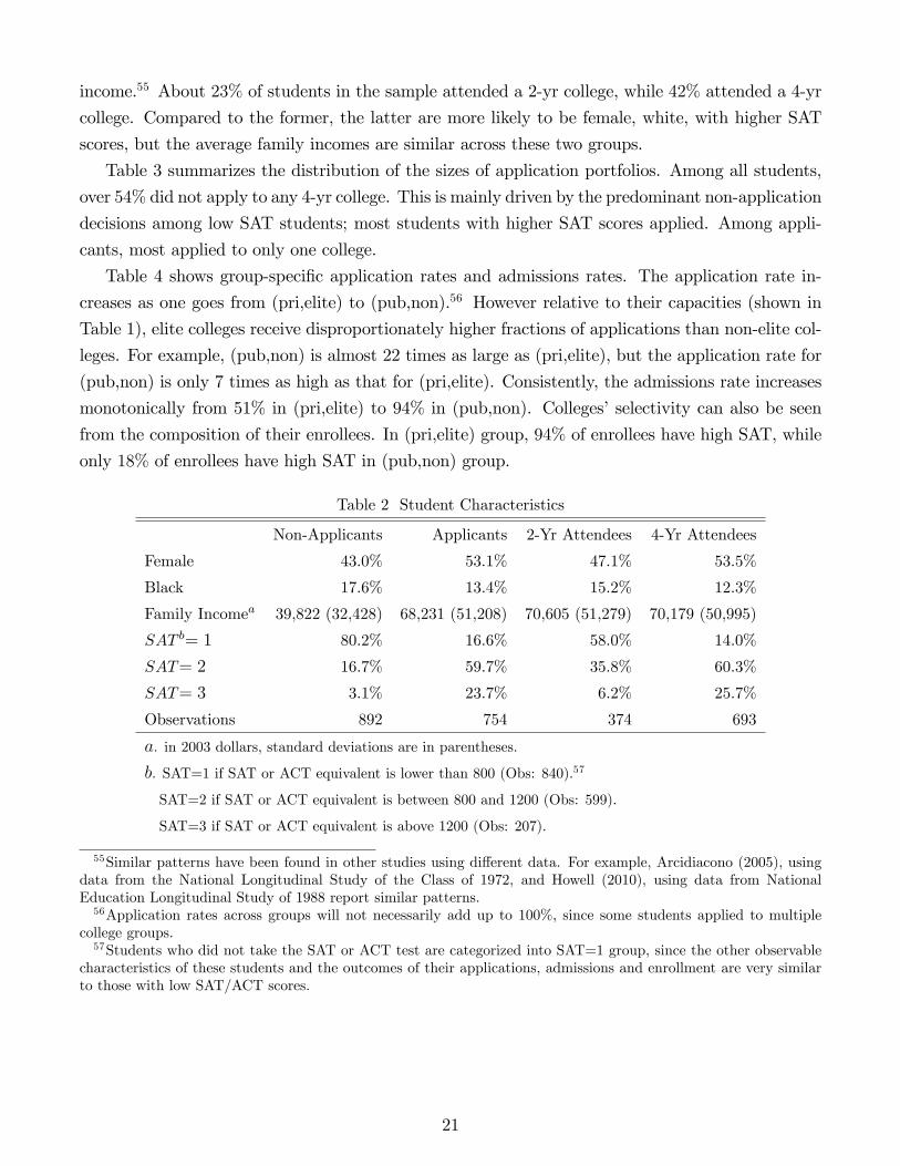
income.55 About 23% of students in the sample attended a 2-yr college, while 42% attended a 4-yr

college. Compared to the former, the latter are more likely to be female, white, with higher SAT

scores, but the average family incomes are similar across these two groups.

Table 3 summarizes the distribution of the sizes of application portfolios. Among all students,

over 54% did not apply to any 4-yr college. This is mainly driven by the predominant non-application

decisions among low SAT students; most students with higher SAT scores applied. Among appli-

cants, most applied to only one college.

Table 4 shows group-speci�c application rates and admissions rates. The application rate in-

creases as one goes from (pri,elite) to (pub,non).56 However relative to their capacities (shown in

Table 1), elite colleges receive disproportionately higher fractions of applications than non-elite col-

leges. For example, (pub,non) is almost 22 times as large as (pri,elite), but the application rate for

(pub,non) is only 7 times as high as that for (pri,elite). Consistently, the admissions rate increases

monotonically from 51% in (pri,elite) to 94% in (pub,non). Colleges�selectivity can also be seen

from the composition of their enrollees. In (pri,elite) group, 94% of enrollees have high SAT, while

only 18% of enrollees have high SAT in (pub,non) group.

Table 2 Student Characteristics

Non-Applicants Applicants 2-Yr Attendees 4-Yr Attendees

Female 43.0% 53.1% 47.1% 53.5%

Black 17.6% 13.4% 15.2% 12.3%

Family Incomea 39,822 (32,428) 68,231 (51,208) 70,605 (51,279) 70,179 (50,995)

SAT b= 1 80.2% 16.6% 58.0% 14.0%

SAT= 2 16.7% 59.7% 35.8% 60.3%

SAT= 3 3.1% 23.7% 6.2% 25.7%

Observations 892 754 374 693

a. in 2003 dollars, standard deviations are in parentheses.

b. SAT=1 if SAT or ACT equivalent is lower than 800 (Obs: 840).57

SAT=2 if SAT or ACT equivalent is between 800 and 1200 (Obs: 599).

SAT=3 if SAT or ACT equivalent is above 1200 (Obs: 207).

55Similar patterns have been found in other studies using di¤erent data. For example, Arcidiacono (2005), usingdata from the National Longitudinal Study of the Class of 1972, and Howell (2010), using data from NationalEducation Longitudinal Study of 1988 report similar patterns.56Application rates across groups will not necessarily add up to 100%; since some students applied to multiple

college groups.57Students who did not take the SAT or ACT test are categorized into SAT=1 group, since the other observable

characteristics of these students and the outcomes of their applications, admissions and enrollment are very similarto those with low SAT/ACT scores.

21

Table 3 Number of Applications (%)

n = 0 n = 1 n � 2All Students 54:2 28:0 17:8

SAT = 1 85:1 12:1 2:8

SAT = 2 24:9 45:2 29:9

SAT = 3 13:0 43:0 44:0

Table 4 Application & Admission: All Applicants

(%) (pri,elite) (pub,elite) (pri,non) (pub,non)

Application Rate 9:7 31:8 44:6 71:5

Admission Rate 53:4 83:0 91:4 94:0

SAT=3 Enrollees 93:8 36:2 27:9 17:8

Num of all applicants: 754

Application rate=num. of group-speci�c applications/num. of all applications

Admission rate=num. of group-speci�c admissions/num. of group-speci�c applications

One pattern not shown in the tables is students�home bias: 66% of all 4-yr applicants applied

to in-state colleges only, and 76% of all 4-yr attendees went to in-state colleges. This can be partly

explained by the tuition di¤erences shown in Table 5, where the within-group average tuition is

based on information from the Integrated Postsecondary Education Data System (IPEDS). Public

colleges price-discriminate against out-of-state students by charging them 3 times as much as they

do in-state students, although still lower than tuition charged by private colleges. The last two rows

summarize �nancial aid data. Relative to students admitted to elite colleges, a higher fraction of

students admitted to non-elite colleges receive college �nancial aid. In addition, 40% of admitted

students receive some outside �nancial aid that helps to fund college attendance in general.

Table 5 Tuition and Financial Aid

(pri,elite) (pub,elite) (pri,non) (pub,non) 2-yr College General

Tuitiona(In-State)

(out-of-state)27; 033

5; 000

14; 43517; 296

3; 969

10; 215

2; 744

��

Aid Recipientsb 25% 24:1% 49:5% 27:2% � 39:9%

Average Aid O¤ered 12; 440 6; 962 11; 389 5; 208 3; 095 4; 326

a. Tuition and aid are measured in 2003 dollars.

b. Num. of aid o¤ers/num. of admissions in the sample. N/A for 2-yr colleges due to open admissions.

5 Empirical Results

Based on the likelihood ratio test, I report the results for the model where in-state and out-of-state

students with the same (SAT;A) face the same admissions probabilities.

22

5.1 Parameter Estimates

5.1.1 Student Preferences for Colleges

Table 6 Preferences for Colleges

($1; 000) (pri,elite) (pub,elite) (pri,non) (pub,non) 2-yr

ug(A=1,z=1)a �187:7 (188:0) �183:2 (5:1) �123:5 (3:8) �188:6 (4:4) �38:1 (1:7)ug(A=2,z=1) �42:2 (66:5) �37:2 (4:6) 31:0 (1:4) 56:8 (2:1) 36:1 (1:4)

ug(A=3,z=1) �52:8 (21:4) 127:3 (0:4) 8:2 (7:6) 73:2 (3:9) 9:8 (4:5)

ug(A=2,z=2) �74:4 (29:4) �115:7 (34:9) 96:6 (4:6) 19:4 (3:19) �13:3 (5:6)ug(A=3,z=2) 139:9 (14:3) 30:4 (14:5) 35:6 (19:5) �66:2 (16:4) �12:7 (33:2)�2�1g (college group) 49:9 (8:4) 24:9 (3:0) 42:3 (1:0) 57:4 (1:8) 61:4 (1:2)

�2�2 (speci�c college) 61:5 (1:2)a The restriction ug(A=1,z=2) = ug(A=1,z=1) holds at 10% signi�cance level.

There is signi�cant heterogeneity in students preferences for colleges, both across student types

and within each type. Rows 1 to 5 of Table 6 show the values of college groups for an average student

of a given type, relative to the non-college option. For an average low-ability (A=1) student, the

non-college option is better than any college option. This explains why the majority of (low family

income, low SAT) students, who are most likely to be of low ability, do not apply to or attend any

college in the data. Due to their low family income, these students would obtain very generous

�nancial aid if they were admitted to any college. Moreover, from an individual student�s point

of view, there is a nontrivial probability that she would be admitted to some college. Given the

apparent "unclaimed" bene�ts for these students, their predominant choices of the non-college

option indicate that the values of colleges must be low for most of them, a �nding consistent with

previous literature such as Cunha, Heckman and Navarro (2005).58 ;59

In most cases, middle-A students rank non-elite colleges over elite colleges, while the opposite is

true for high-A students. Such patterns are not completely surprising. For example, it is reasonable

to believe that the e¤ort costs required in elite colleges are higher than those required in non-elite

colleges, and that these costs decrease with student ability. Considering the e¤ort costs and the

probabilities of success in di¤erent colleges, a mediocre student might be better o¤ attending a

58Cunha, Heckman and Navarro (2005) �nd very high psychic costs of attending college (median around $500; 000),which stand in for expectational errors and attitudes towards risk that explain why agents who face high gross returnsdo not go to college.59Another potential but perhaps minor explanation is borrowing constraint. For example, Cameron and Heckman

(1998) and Keane and Wolpin (2001), �nd that borrowing constraints have a negligible impact on college attendance,based on which I assume no borrowing constraint. Lochner and Monge-Naranjo (2011) �nd that conditional onAFQT, the correlation between family income and college attendance is weaker for the NLSY79 cohort than for theNLSY97 cohort, suggesting the later cohort may be more constained. Alternatively, their �nding can be explainedby the stronger correlation between family income and students�college ability, even after controlling for AFQT.That is, there are more students from the later cohorts that are constrained in their childhood when their pre-collegehuman capital is formed.

23

non-elite college.

Holding ability constant, z-1 type in general value public and 2-yr colleges over private colleges,

while the opposite holds for z-2 type. Private colleges and public colleges have di¤erent features

that may �t some students better than others. For example, private colleges are usually smaller

than public colleges, which may be an advantage for some students but a disadvantage for others.

By introducing types, the model explains the systematic di¤erences in students�choices. The

residual non-systematic di¤erences in student choices are accounted for by their idiosyncratic pref-

erences, which feature signi�cant dispersions both for college groups (��1g) and for speci�c colleges

(��2). In sum, not only do students attach di¤erent values to the same college, but they also rank

colleges di¤erently. For example, attending an elite college is not optimal for all students.60 Instead,

each option (including the outside option) o¤ered in the college market best caters to some groups

of students.

5.1.2 Home Bias

Table 7 shows the disutility of attending colleges out of one�s home state, which includes both

extra monetary costs such as costs for transportation and residence, as well as psychic cost.61 Such

costs are found to be lower for high-A students, who are presumably better at adapting to new

environment. Students who prefer public colleges over private colleges (z = 1) exhibit greater

unwillingness to study far away from home. The identi�cation of type-speci�c home biases comes

from the correlation of student choices and their characteristics. For example, the fraction of

applicants who applied only within home states is 50% among high-SAT applicants, as compared

to 70% among other applicants. Similarly, controlling for the number of applications, for example

at 2, the fraction of applicants who applied only within home states is 50% among students who

applied to at least one private college, as compared to 64% among those who only applied for public

colleges. Finally, the dispersion of student decisions to apply out of state among similar students

identi�es ��.

Table 7 Out-of-State Utility Cost

$1; 000 (A=3,z=2) (A<3,z=2) (A=3,z=1) (A<3,z=1)

Mean (�K) 22:5 (1:1) 26:1 (0:6) 37:1 40:7

�(A,z=1)��(A,z=2) 14:6 (0:5)

Dispersion (��) 35:1 (0:5)a The restriction �(A=1,z)=�(A=2,z) holds at 10% signi�cance level.

Remark All three taste dispersions, across college groups (��1g), speci�c colleges (��2) and home

bias (��), are necessary to explain the data. For example, suppose ��2 = 0, the following application

60This is consistent with �ndings from some other studies, for example, Dale and Krueger (2002).61Studies on migration decisions often �nd that both the mean and the dispersion of moving costs are substantial.

For example, Kennan and Walker (2011).

24

pro�le would not happen, where a student applied to two colleges, one out-of-state public and the

other in-state private. The fact that she applied to an out-of-state public college, willing to pay

out-of-state tuition, but not an in-state counterpart, reveals her taste for studying out of home

state. However, if that is the case, she should not have chosen an in-state private college over an

out-of-state counterpart. It is cases like this that identify ��2.

5.1.3 Application Costs

Table 8 Application Costs

$1; 000 n = 1 n = 2 n = 3 n � 4C(n)� C(n� 1) 1:90 (0:3) 0:90 (0:05) 0:33 (0:02) 0:27 (0:03)

The cost for the �rst application is about $1; 900, but as the number of applications increases, the

marginal cost rapidly decreases, suggesting the existence of some economies of scale. In interpreting

application costs, on the one hand, one must remember that they incorporate all factors that make

application costly, i.e., all student-side barriers to applying for colleges other than their ability

and preferences. For example, the cost to collect information and prepare application materials,

the stress to meet the application deadlines, and the anxiety felt while waiting for admissions

results. On the other hand, student ability and preferences are far more important in explaining

the application patterns found in the data. As an example, if one �xes all the other parameters

and reduces application costs by half and simulate the student decision model, the fraction of

non-applicants remains at 51%, as compared to 54% in the baseline model. For many students,

application costs are irrelevant to their decisions. For example, average low-ability students, who

derive negative utilities from colleges, will not apply even if application is costless.

The same cannot be said for students that are at the margin of applying and not applying,

applying more and applying less. For example, since SAT is only a noisy measure of student ability,

students of the same type may have di¤erent SAT scores, hence di¤erent admissions probabilities.

Were application costs negligible, there should not be noticeable adjustment in their application

choices to the admissions probabilities, since they share the same preferences on average. The extent

to which such adjustment exists informs one of the importance of application costs.62

5.1.4 Ability Measures

One important feature of this model is information friction: students can only convey their abilities

to colleges via noisy ability measures. The following two tables show the severity of such information

friction. Based on the ability distribution parameter estimates, each row of Table 9.1 shows the

distribution of SAT scores given ability, where each row adds up to 100%. Over 90% of the cases,

Ability-1 students will score low in SAT, which makes it relatively easy to distinguish them from

62See the appendix for details.

25

the others based on SAT. However, SAT is less useful in distinguishing between medium-ability and

high-ability types.

Table 9.1 SAT and Ability: Simulation

% P (SAT= 1jA) P (SAT= 2jA) P (SAT= 3jA)A = 1 91:0 8:3 0:7

A = 2 18:3 65:8 15:9

A = 3 1:5 52:4 46:1

Table 9.2 reports the distribution of signals conditional on ability. Ability-2 students distinguish

themselves from Ability-1 students primarily by their low probability of sending out low signals.

Ability-3 students are much more likely than others to send high signals, and almost never send out

low signals.63

Table 9.2 Signal Distribution

% P (s = 1jA) P (s = 2jA) P (s = 3jA)A = 1 94:1 (0:4) 1:4 4:5 (5:1)

A = 2 7:7 (0:5) 87:8 4:6 (2:4)

A = 3 0:04 (0:7) 46:7 53:3 (8:8)

Previous studies, for example, Cameron and Heckman (2001), have noted that family income

has substantial in�uence on forming students�ability. Table 9.3 reinforces this �nding by showing

ability distribution among di¤erent family income groups, where each column adds up to 100%.

Students from low income families are most likely to be of low ability, and hence very low preferences

for colleges. The e¤ect of such preferences on college attendance will be illustrated in the �rst

counterfactual experiment.

Table 9.3 Family Income and Ability

% P (AjLow Inc) P (AjMiddle Inc) P (AjHigh Inc)A = 1 71:8 49:8 20:8

A = 2 25:1 40:2 49:6

A = 3 3:1 10:0 26:7

Low Inc: if family income is below 25th percentile (group mean $10,017)

Middle Inc: if family income is in 25-75th percentile (group mean $45,611)

High Inc: if family income is above 75th percentile (group mean $110,068)

5.2 Model Fit

Given the parameter estimates, I simulate the subgame perfect Nash equilibrium model (SPNE)

and compare model predictions with the data.64 Tables 10 shows the number of applications.63Table G1.4 in the appendix shows the distribution of ability, SAT and signals among applicants.64Model �ts by SAT and by family income are in the appendix.

26

Table 11 shows the allocation of these applications and the admissions rates by college groups.

Table 12 displays the �ts of student �nal allocation in terms of college groups: the model slightly

under-predict the fraction of students attending non-elite colleges. As Table 13 shows, the model

replicates the pattern that most applications and attendance occur within home states. Finally,

Table 14 contrasts model predicted tuition levels with the data.

Table 10 Model v.s. Data

Num of Applications (%)

Size Data Model

0 54:2 54:5

1 28:0 27:8

2 or more 17:8 17:7

�2 Stat 0:06

�22;0:05= 5:99

Table 11 Model v.s. Data

Application & Admission: Applicants (%)

Application Rate Data Model

(pri,elite) 9:7 9:4

(pub,elite) 31:8 29:0

(pri,non) 44:6 44:4

(pub,non) 71:5 67:6

Admission Rate

(pri,elite) 53:4 58:5

(pub,elite) 83:0 90:1

(pri,non) 91:4 91:5

(pub,non) 94:0 95:9� All Pass �21;0:05 test.

27

Table 12 Model v.s. Data

Final Allocation of Students (%)

Data Model

(pri,elite) 1:0 1:5

(pub,elite) 7:7 8:0

(pri,non) 11:5 10:9

(pub,non) 21:9 20:2

2-yr college 22:7 22:9

Non-college 35:2 36:5

�2 Stat. 6:98

�25;0:05=11:07

Table 13 Model v.s. Data: Home Bias

% Data Model

Home-Only Applicantsa 65:6 67:5

Home-State Attendeesb 76:2 78:0� Both pass �21;0:05 test.a % students who apply only within home states among all 4-yr applicants.b % students who attend home-state 4-yr colleges among all 4-yr attendees.

Table 14 Model v.s. Data: Tuition

$ (pri,elite) (pub,elite) (pri,non) (pub,non)

In-State Out-of-State In-State Out-of-State

Data 27; 033 5; 000 14; 435 17; 296 3; 969 10; 215

Model 27; 530 5; 090 13; 892 16; 891 3; 451 10; 540

6 Counterfactual Experiments

With the estimated model, I conduct two counterfactual experiments. Comparisons are made

between the baseline SPNE and the new SPNE.65

6.1 Creating More Opportunities

To what extent can the government expand college access by increasing college capacities? To

answer this question, I consider two counterfactual scenarios. In the �rst, community college tuition

is maintained at its current level ($2; 744), which also serves as the lower bound for 4-yr college

65In simulating the baseline model and the counterfactual experiments, I tried a wide range of initial guesses inmy search for equilibrium. For each model, I �nd only one equilibrium.

28

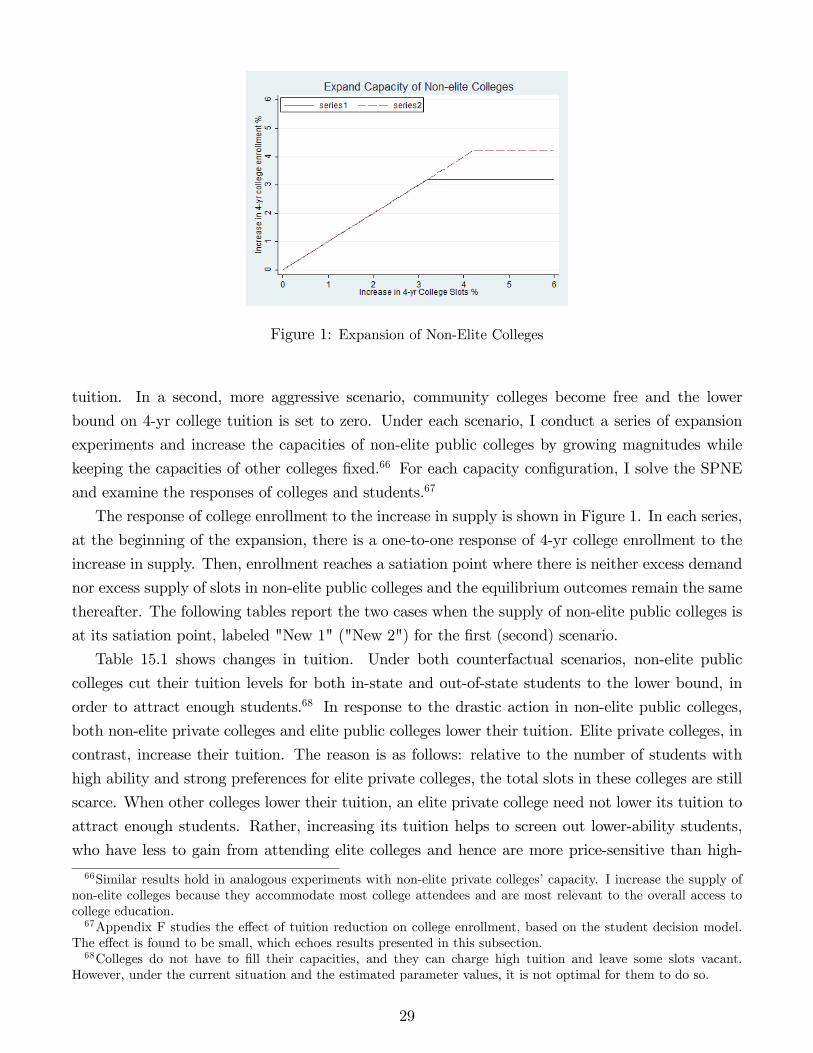
Figure 1: Expansion of Non-Elite Colleges

tuition. In a second, more aggressive scenario, community colleges become free and the lower

bound on 4-yr college tuition is set to zero. Under each scenario, I conduct a series of expansion

experiments and increase the capacities of non-elite public colleges by growing magnitudes while

keeping the capacities of other colleges �xed.66 For each capacity con�guration, I solve the SPNE

and examine the responses of colleges and students.67

The response of college enrollment to the increase in supply is shown in Figure 1. In each series,

at the beginning of the expansion, there is a one-to-one response of 4-yr college enrollment to the

increase in supply. Then, enrollment reaches a satiation point where there is neither excess demand

nor excess supply of slots in non-elite public colleges and the equilibrium outcomes remain the same

thereafter. The following tables report the two cases when the supply of non-elite public colleges is

at its satiation point, labeled "New 1" ("New 2") for the �rst (second) scenario.

Table 15.1 shows changes in tuition. Under both counterfactual scenarios, non-elite public

colleges cut their tuition levels for both in-state and out-of-state students to the lower bound, in

order to attract enough students.68 In response to the drastic action in non-elite public colleges,

both non-elite private colleges and elite public colleges lower their tuition. Elite private colleges, in

contrast, increase their tuition. The reason is as follows: relative to the number of students with

high ability and strong preferences for elite private colleges, the total slots in these colleges are still

scarce. When other colleges lower their tuition, an elite private college need not lower its tuition to

attract enough students. Rather, increasing its tuition helps to screen out lower-ability students,

who have less to gain from attending elite colleges and hence are more price-sensitive than high-

66Similar results hold in analogous experiments with non-elite private colleges�capacity. I increase the supply ofnon-elite colleges because they accommodate most college attendees and are most relevant to the overall access tocollege education.67Appendix F studies the e¤ect of tuition reduction on college enrollment, based on the student decision model.

The e¤ect is found to be small, which echoes results presented in this subsection.68Colleges do not have to �ll their capacities, and they can charge high tuition and leave some slots vacant.

However, under the current situation and the estimated parameter values, it is not optimal for them to do so.

29

ability students. Therefore, even though an elite private college compete with colleges both in other

groups and within its own group, increasing tuition is a good strategy. None of the other colleges,

including the elite public, enjoy such market power: competition forces them to lower tuition.

Table 15.1 Increasing Supply: Tuition

$ (pri,elite) (pub,elite) (pri,non) (pub,non)

In-State Out-of-State In-State Out-of-State

Baseline 27; 530 5; 090 13; 892 16; 891 3; 451 10; 540

New 1 29; 152 4; 177 11; 568 15; 291 2; 744 2; 744

New 2 29; 952 2; 917 7; 308 13; 631 0 18

In both counterfactual cases, the expanded non-elite public colleges admit all of their applicants.

Under Scenario 1, admissions rates also increase in all the other colleges. The major driving forces

for the increased admissions rates are likely to di¤er across college groups. For colleges other than

the elite private, higher admissions rates and lower tuition re�ect their e¤orts to enroll enough

students. The elite private colleges increase their admissions rates mainly because they are faced

with a better self-selected applicant pool, as a result of the enlarged tuition gap. Under Scenario 2,

elite private colleges continue to increase both their tuition and admissions rates. The admissions

rates in elite public colleges and non-elite private colleges are slightly lower than their baseline levels

due to their dramatic tuition reduction.

Table 15.2 Increasing Supply: Admissions

% (pri,elite) (pub,elite) (pri,non) (pub,non)

Baseline 58:5 90:1 91:5 95:9

New 1 63:6 90:8 92:1 100:0

New 2 71:8 89:8 91:3 100:0

Table 15.3 displays the attendance rates among all students. In Scenario 1, 4-yr college atten-

dance rate increases by 2:6%, while 2-yr colleges lose 1% of their enrollees. In Scenario 2, 3:6% more

students are drawn into colleges. Since the supply of non-elite public colleges exceeds demand if

they are enlarged further, these increases represent the upper limits to which the government can

increase college attendance by such expansions.

Table 15.3 Increasing Supply: Attendance

% Baseline New 1 New 2 All Open&Free

4-Yr 40:6 43:2 44:2 55:6

2-Yr 22:9 21:9 22:9 18:0

I also conduct a partial equilibrium experiment where all colleges are open and free. This is an

extreme situation with unlimited supply of all colleges. The result is reported in the last column of

Table 15.3. Four-year college attendance rate increases by 15%. Two-year colleges lose 5% of their

30

enrollees, however, most of their enrollees choose to stay instead of attending 4-yr colleges for free,

highlighting the importance of 2-yr colleges. Considering total college enrollment, some students

(10%) are indeed constrained by tuition and/or available slots. However, the vast majority of

students who do not attend college under the base SPNE prefer the outside option over any college

option.

To explain why expansion has such limited e¤ects on enrollment, Table 15.4 shows the attendance

rates by student ability. Under the baseline, only 28% of low-ability students attend any college

and almost none attend 4-yr colleges. When all colleges become free and open, 18% more of them

will be attracted to colleges, while the majority still choose the non-college option. In contrast,

almost all students of higher ability attend colleges, mostly 4-yr ones. Therefore, the major barrier

to college access is student ability and associated preferences, not college capacity or tuition.69

Table 15.4 Increasing Supply: Attendance by Ability

% Baseline New 1 New 2 All Open&Free

A = 1

4-Yr 1:0 3:5 4:3 18:9

2-Yr 27:0 26:5 29:2 26:5

A = 2

4-Yr 72:3 75:1 76:7 86:9

2-Yr 24:0 21:9 21:1 12:7

A = 3

4-Yr 93:3 94:1 94:4 97:8

2-Yr 5:8 5:3 5:1 2:2

6.2 Ignoring Signals

In some countries, such as China, college admissions are based almost entirely on scores in a nation-

wide test. Although such a system may save resources invested in the admissions process, such

as the human resource employed in reading thousands of student essays, it ignores a valuable

source of information about student ability. In the second counterfactual experiment, I assess the

consequences of ignoring signals in the admissions process.70

Table 16.1 shows the changes in tuition under the new SPNE. Elite colleges draw on higher

tuition to screen students when the information on ability provided by signals becomes unavailable,

because their target enrollees, i.e., high-ability students, are less price-sensitive. However, the

screening e¤ect of tuition is not strong enough to make up for the loss of information embedded

69This �nding is in line with earlier research. See, for example, Cameron and Heckman (1998, 2001) and Keaneand Wolpin (2001).70In a di¤erent counterfactual experiment, I examine the opposite case, where admission o¢ ces can only use student

signals to distinguish between applicants. The results are similar. For example, elite (non-elite) colleges increase(decrease) their tuition. Details are available upon request.

31

in signals, and more high-ability applicants will be mistakenly rejected by elite colleges. Knowing

this fact, non-elite colleges lower their tuition to compete for these students, who apply to them as

insurance.

Table 16.1 Ignore Signals: Tuition

$ (pri,elite) (pub,elite) (pri,non) (pub,non)

In-State Out-of-State In-State Out-of-State

Baseline 27; 530 5; 090 13; 892 16; 891 3; 451 10; 540

New 30; 028 5; 131 14; 079 14; 800 3; 083 9; 426

In response to these tuition reductions, more students apply to colleges (Table 16.2). However,

applicants apply less. As admissions only depend on SAT and students know their SAT scores,

there is less uncertainty hence less need for portfolio diversi�cation. The reduction in uncertainty

is especially true for high-SAT applicants, who are now admitted in all colleges (Table 16.3). The

overall admissions rates, however, decrease in all colleges, due to the low admissions rates among

low-SAT applicants.

Table 16.2 Ignore Signals: Num of Applications

% Num = 0 Num = 1 Num � 2Baseline 54:5 27:8 17:7

New 52:7 34:2 13:1

Table 16.3 Ignore Signals: Admission Rates

% All SAT= 1 SAT= 2 SAT= 3

Base New Base New Base New Base New

(pri,elite) 58:5 66:7 22:1 N=A 41:3 32:9 76:2 100:0

(pub,elite) 90:1 88:9 16:0 6:5 91:0 100:0 98:0 100:0

(pri,non) 91:5 80:0 77:1 11:2 93:7 100:0 100:0 100:0

(pub,non) 95:9 90:6 83:1 62:3 98:5 100:0 100:0 100:0

*N/A: not applicable because of zero applicant.

With less information available, elite colleges experience a drop in their enrollee ability, while the

non-elite ones get more high-ability students (Table 16.4). As shown in Table 16.5, average student

welfare decreases by $600. Both middle-ability and high-ability students lose. The only winners

are low-ability students, who gain because colleges �nd it harder to distinguish these students from

others.

Table 16.4 Ignore Signals: % of High-Ability Students

% (pri,top) (pub,top) (pri,non) (pub,non)

Baseline 94:7 80:2 11:0 15:9

New 86:4 79:0 12:7 16:1

32

Table 16.5 Ignore Signals: Student Welfare

$1; 000 Baseline New

All 67:8 67:2

A = 1 10:4 11:3

A = 2 111:0 109:0

A = 3 150:4 148:8

7 Conclusion

In this paper, I have developed and structurally estimated an equilibrium model of the college

market. It provides a �rst step toward a better understanding of the college market by jointly

considering tuition setting, applications, admissions and enrollment. In the model, students are

heterogeneous in their abilities and preferences. They face uncertainty and application costs when

making their application decisions. Colleges, observing only noisy measures of student ability,

compete for more able students via tuition and admissions policies. I have estimated the structural

model via a three-step estimation procedure to cope with the complications caused by potential

multiple equilibria. The empirical results suggest that the model closely replicates most of the

patterns in the data.

My empirical analyses suggest that, �rst, there is substantial heterogeneity in students�pref-

erence for colleges. Expanding college capacities has very limited e¤ects on college attendance:

neither tuition cost nor college capacity is a major obstacle to college access; a large fraction of

students, mainly low-ability students, prefer the outside option over any college option. Second,

there are signi�cant amounts of noise in various types of ability measures. When colleges lose access

to one measure of student ability, elite colleges draw on higher tuition to help screen students, while

non-elite colleges lower their tuition to compete for high-ability students who apply for them as

insurance.

The methods developed in this paper and the main empirical �ndings are promising for future

research. Building on Epple, Romano and Sieg (2006) and this paper, a model that endogenizes

applications, admissions and �nancial aid would provide a more comprehensive view of the college

market. Building on Arcidiacono (2005) and this paper, a model that studies the strategic interac-

tions between colleges and students and links them to students�labor market outcomes would also

be an important extension. The latter will become feasible as more information of students�labor

market outcomes becomes available from future surveys of the NLSY97.

Another important direction for future research is to study the long-run equilibrium in order

to obtain a better understanding of the trend of college tuition and attendance. In a long run

equilibrium model, one can be more explicit about why colleges value student ability. For example,

higher-ability students are more likely to do better in the job market, which enhances the college�s

prestige and attractiveness to future applicants. Moreover, building on this paper and the studies

33

on childhood human capital formation, such as Cunha, Heckman and Schennach (2010), one can

also be more speci�c about how student preferences for colleges are formed and how childhood

investment decisions might a¤ect and be a¤ected by the college market. That is, although students�

evaluations of colleges are taken as given in the short run, in the long run, these evaluations will

evolve as an equilibrium outcome.

Finally, one can also endogenize college capacities in the long run. One approach to implement

this extension is to introduce a cost function for college education, assuming free entry to the

market. Equilibrium of the model would then depend on the form of the cost function. Estimation

of such a model would require additional data on college expenses and non-tuition revenues, as well

as application and admissions data over multiple years.

References

Arcidiacono, Peter. 2005. "A¢ rmative Action in Higher Education: How Do Admission and Finan-

cial Aid Rules A¤ect Future Earnings?" Econometrica, 73(5): 1477-1524.

Arcidiacono, Peter and Sean Nicholson. 2005. "Peer e¤ects in medical school." Journal of Public

Economics, 89(2-3): 327-350

Avery, Christopher, Andrew Fairbanks and Richard Zeckhauser. 2003. The Early Admissions Game:

Joining the Elite. Cambridge, MA: Harvard University Press.

Avery, Christopher, Jonathan Levin. 2010. "Early Admissions at Selective Colleges." American

Economic Review, 100(6): 1-34.

Bajari, Patrick, C. Lanier Benkard and Jonathan Levin. 2007. "Estimating Dynamic Models of

Imperfect Competition." Econometrica, 75(5): 1331�1370.

Bajari, Patrick, Han Hong, John Krainer and Denis Nekipelov. 2010. "Estimating Static Models of

Strategic Interactions." Journal of Business and Economic Statistics, 28(4): 469-482.

Berry, Steven, James Levinsohn and Ariel Pakes. 1995. "Automobile Prices in Market Equilibrium."

Econometrica, 63(4): 841-890.

Berry, Steven, James Levinsohn and Ariel Pakes. 2004. "Di¤erentiated Products Demand Systems

from a Combination of Micro andMacro Data: The New CarMarket." Journal of Political Economy,

112 (1): 68-104.

Bowen, William and Derek Bok. 1998. The Shape of the River: Long-Term Consequences of Con-

sidering Race in College and University Admissions. Princeton, NJ: Princeton University Press.

Bresnahan, Timothy and Peter Reiss. 1990. "Entry in Monopoly Markets." The Review of Economic

Studies, 57: 531-553.

34

Chade, Hector, Gregory Lewis and Lones Smith. 2011. "Student Portfolios and the College Admis-

sions Problem." Social Science Research Network Working Paper 135834.

Cameron, Stephen and James Heckman. 1998. �Life Cycle Schooling and Dynamic Selection Bias:

Models and Evidence for Five Cohorts of American Males.�Journal of Political Economy, 106(2):

262-333.

Cameron, Stephen and James Heckman. 2001. �The Dynamics of Educational Attainment for Black,

Hispanic, and White Males.�Journal of Political Economy, 109(3): 455-499.

Ciliberto, Federico and Elie Tamer. 2009. "Market Structure and Multiple Equilibria in Airline

Markets." Econometrica, 77(6): 1791-1828.

Cunha, Flavio, James Heckman and Salvador Navarro. 2005. "Separating Heterogeneity from Un-

certainty in Life Cycle Earnings." Oxford Economic Papers, Vol. 57(2): 191-261.

Cunha, Flavio, James Heckman, and Susanne Schennach. 2010. "Estimating the Technology of

Cognitive and Noncognitive Skill Formation." Econometrica, 78(3): 883�931.

Dale, Stacy and Alan Krueger. 2002. "Estimating The Payo¤ To Attending A More Selective Col-

lege: An Application Of Selection On Observables And Unobservables." The Quarterly Journal of

Economics, 117(4): 1491-1527.

de Paula, Aureo. 2013 "Econometric Analysis of Games with Multiple Equilibria." Annual Review

of Economics, 5: 107-131.

Epple, Dennis, Richard Romano and Holger Sieg. 2006. "Admission, Tuition, And Financial Aid

Policies in The Market For Higher Education." Econometrica, 74(4): 885-928.

Howell, Jessica. 2010. "Assessing the Impact of Eliminating A¢ rmative Action in Higher Educa-

tion." Journal of Labor Economics, 28(1): 113-166.

Kane, Thomas. 1998. �Racial and Ethnic Preferences in College Admissions.�in The Black-White

Test Score Gap, ed. Christopher Jencks and Meredith Phillips, 971-996. Washington D.C.: Brook-

ings Institution Press.

Keane, Michael and Kenneth Wolpin. 2001. "The E¤ect of Parental Transfers and Borrowing Con-

straints on Educational Attainment." International Economic Review, 42(4): 1051-1103.

Kennan, John and James Walker. 2011. "The E¤ect of Expected Income on Individual Migration

Decisions." Econometrica, 79(1): 211�251.

Leslie, Larry, and Paul Brinkman. 1998. The Economic Value of Higher Education. New York:

Macmillan.

35

Lewbel, Arthur. 2000. "Semiparametric qualitative response model estimation with unknown het-

eroscedasticity or instrumental variables." Journal of Econometrics, 97: 145-177.

Light, Audrey and Wayne Strayer. 2002. �From Bakke to Hopwood: Does Race A¤ect College

Attendance and Completion?�The Review of Economics and Statistics, 85: 34-44.

Lochner, Lance and Alexander Monge-Naranjo. 2011. "The Nature of Credit Constraints and Hu-

man Capital" American Economic Review, 101(6): 2487-2529.

Mailath, George, Masahiro Okuno-Fujiwara and Andrew Postlewaite. 1993. "Belief-Based Re�ne-

ments in Signalling Games." Journal of Economic Theory, 60: 241-276.

Manski, Charles and David Wise. 1983. College Choice in America. Cambridge, MA: Harvard

University Press

McFadden, Daniel. 1989. �A Method of Simulated Moments for Estimation of Discrete Response

Models without Numerical Integration.�Econometrica, 57(5): 995-1026.

Meijer, Erik and Jelmer Ypma. 2008. "A Simple Identi�cation Proof for a Mixture of Two Univariate

Normal Distributions." Journal of Classi�cation, 25: 113-123.

Moro, Andrea. 2003. �The E¤ect of Statistical Discrimination on Black-White Wage Di¤erentials:

Estimating a Model with Multiple Equilibria.�International Economic Review, 44(2): 467-500.

Nagypál, Eva. 2004. "Optimal Application Behavior with Incomplete Information." mimeo, North-

western University.

Rothschild, Michael and Lawrence White. 1995. "The Analytics of the Pricing of Higher Education

and Other Services in Which the Customers Are Inputs." Journal of Political Economy, 103(3):

573-586.

Sacerdote, Bruce. 2001. �Peer E¤ects with Random Assignment: Results from Dartmouth Room-

mates.�Quarterly Journal of Economics, 116: 681�704.

Tamer, Elie. 2003. "Incomplete Simultaneous Discrete Response Model with Multiple Equilibria."

The Review of Economic Studies, 70(1): 147-165.

Winston, Gordon. 1999. "Subsidies, Hierarchy and Peers: The Awkward Economics of Higher

Education." Journal of Economic Perspectives, 13(1): 13-36.

Zimmerman, David. 2003. �Peer E¤ects in Higher Education: Evidence from a Natural Experi-

ment.�The Review of Economics and Statistics, 85: 9�23.

APPENDIX:

36

A. Model Details:A1. College Admissions ProblemThe following formally derives a college�s optimal admissions policy without discrimination based

on student origin.71 Given tuition pro�le t, students�strategies Y (�); d(�)and other colleges�admis-sions policies e�j, college j solves the following problem:

maxej(s;SAT jt)

(Xs;SAT

ej(s; SAT jt)�j(s; SAT jt; e�j; Y; d)�j(s; SAT j�) j(s; SAT j�))

(12)

s:t:Xs;SAT

ej(s; SAT jt)�j(s; SAT jt; e�j; Y; d)�j(s; SAT j�) � �j

ej(s; SAT jt) 2 [0; 1];

where ej(s; SAT jt) is college j�s admissions policy for its applicants with (s; SAT ), �j(s; SAT jt; e�j; Y; d)is the probability that such an applicant will accept college j�s admission. j(s; SAT jt; e�j; Y; d) isthe expected ability of such an applicant conditional on her accepting j�s admission. �j(s; SAT jt; e�j; Y; d) isthe measure of j�s applicants with (s; SAT ). The �rst order condition for problem (12) is

j(s; SAT j�)� �j + �a � �b = 0;

where �j is the multiplier associated with the capacity constraint, i.e., the shadow price of a slot

in college j. �a and �b are adjusted multipliers associated with the constraint that ej(s; SAT jt) 2[0; 1]:72

If it admits an applicant with (s; SAT )and the applicant accepts the admission, college j must

surrender a slot from its limited capacity, thus inducing the marginal cost �j. The marginal bene�t

is the expected ability of such an applicant conditional on her accepting j�s admission. Balancing

between the marginal bene�t and the marginal cost, the solution to college j�s admissions problem

is characterized by:

ej(s; SAT jt)

8><>:= 1 if j(s; SAT j�)� �j > 0= 0 if j(s; SAT j�)� �j < 02 [0; 1] if j(s; SAT j�)� �j = 0

; (13)

Xs;SAT

ej(s; SAT jt)�j(s; SAT j�)�j(s; SAT j�) � �j; (14)

and

�j

(� 0 if (14) is binding= 0 if (14) is not binding

:

71The derivation of policy with origin-based discrimination is similar: a student�s origin will be observed and theargument in ej (�) ; �j (�) ; �j (�) and j (�) will extend from (s; SAT ) to (s; SAT; I (li = lj)).72�a; �b are the multipliers associated with �j(s; SAT j�)�j(s; SAT j�)ej(s; SAT jt) 2 [0; 1]:

37

To implement its admissions policy, college j will �rst rank its applicants with di¤erent (s; SAT )

by their expected ability conditional on their acceptance of j�s admissions. All applicants with

the same (s; SAT ) are identical to the college and hence are treated equally. Everyone in an

(s; SAT ) group will be admitted if 1) this (s; SAT ) group is ranked highest among the groups

whose admissions are still to be decided, 2) their marginal contribution to the college is positive,

and 3) the expected enrollment of this group is no larger than college j�s remaining capacity, where

j�s remaining capacity equals �j minus the sum of expected enrollment of groups ranked above.

A random fraction of an (s; SAT ) group is admitted if 1) and 2) hold but 3) fails, where the

fraction equals the remaining capacity divided by the expected enrollment of this group. As a

result, a typical set of admissions policies for the ranked (s; SAT ) groups, fej(s; SAT jt)g ; would bef1; :::; 1; "; 0; :::; 0g, with " 2 (0; 1) if the capacity constraint is binding, and f1; :::; 1g if the capacityconstraint is not binding or just binding.

A1.1 Calculating �j(s; SAT jt; e�j; Y; d) and j(s; SAT jt; e�j; Y; d)All objects depend on ft; e�j; Y; dg. To save notation, the dependence is suppressed. Let

Pr(acceptjX;SAT; �; j) be the probability that a student with characteristics (X;SAT; �) whoapplies to College j accepts j�s admission. Let F (X; �js; SAT; j) be the distribution of (X; �)conditional on (s; SAT ) and application to j. The probability that an applicant with (s; SAT )

accepts j�s admission is:

�j(s; SAT j�) =ZPr(acceptjX;SAT; �; j)dF (X; �js; SAT; j).

Let Pr(O�jjA; SAT ) �Yl2Onj

pl(A; SAT )Y

j02Y nO

(1� pj0(A; SAT )) be the probability of admission set

O for a student with (A; SAT ), with college j admitting her for sure,

Pr(acceptjX;SAT; �; j) =X

O�j�Y (X;SAT )nfjg

Pr(O�jjA; SAT )I(j = d(X;SAT; �;O)):

That is, the student will accept j�s admission if j is the best post-application choice for her. The

distribution F (X; �js; SAT; j) is given by

dF (X; �js; SAT; j) =P (sjA)I(j 2 Y (X;SAT ))dH(X; �jSAT )

�j(s; SAT j�);

�j(s; SAT j�) =

ZP (sjA)I(j 2 Y (X;SAT ))dH(X; �jSAT );

where H(X; �jSAT ) is exogenous and equal to the product of type distribution, the distribution ofex-post shocks and the distribution of family backgrounds conditional on SAT .

The expected ability of applicant (s; SAT ) conditional on acceptance is

38

j(s; SAT j�) =RAPr(acceptjX;SAT; �; j)dF (X; �js; SAT; j)

�j(s; SAT j�):

A2. Proof of existence in a simpli�ed model.Assume there are two colleges j 2 f1; 2g and a continuum of students divided into two ability

levels. The utility of the outside option is normalized to 0. The utility of attending college 1 is

u1(A) for all with ability A, and that of attending college 2 is u2(A)+�, where � is i.i.d. idiosyncratic

taste. There are two SAT levels and two signal levels. There is no ex-post shock. Some notations

to be used: for an (A; SAT ) group, let the fraction of students that do not apply to any college

be �0A;SAT , the fraction of those applying to college j only be �jA;SAT and the fraction applying to

both be �12A;SAT . For each (A; SAT ) group, �A;SAT 2 �, a 3-simplex. For all four (A; SAT ) groups,� 2 � � �4. On the college side, each college chooses admissions policy ej 2 [0; 1]4, where 4 is thenumber of (s; SAT ) groups faced by the college.

Proposition 1 For any given tuition pro�le t, an application-admission equilibrium exists.

Proof. Step 1: The application-admission model can be decomposed into the following sub-

mappings:

Taking the distribution of applicants, and the admissions policy of the other college as given, college

j�s problem (12) can be viewed as the sub-mapping

Mj : �� [0; 1]4 � [0; 1]4;

for j = 1; 2. Taking college admissions policies as given, the distribution of students is obtained via

the sub-mapping

M3 : [0; 1]4 � [0; 1]4 ! �:

An equilibrium is a �xed point of the mapping:

M : �� [0; 1]4 � [0; 1]4 � �� [0; 1]4 � [0; 1]4

s:t: � 2 M3(e1;e2)

ej 2 Mj(�; ej0) j; j0 2 f1; 2g; j 6= j0:

Step 2: Show that Kakutani�s Fixed Point Theorem applies in mappingM and hence an equilibrium

exists.

1) The domain of the mapping, being the product of simplexes, is compact and non empty.

2) It can be shown that the correspondence Mj(�; �) is compact-valued, convex-valued and upper-hemi-continuous, for j = 1; 2. In particular, the (s; SAT )�th component ofMj(�; ej0) is characterized

by (13) and (14), where j(s; SAT ) +M(tj;mj)� �j is continuous in (�; ej0):3) Aggregate individual optimization into distribution of students �.

39

Generically, each student has a unique optimal application portfolio as the solution to (6). For

given (A; SAT ), there exist ��(e) � ���(e), both continuous in e, such that:

For � � ��(e), Y (A; SAT; �) =(f2g if C(2)� C(1) > k1(e)f1; 2g otherwise

;

for � 2 [���(e); ��(e)); Y (A; SAT; �) = f1; 2g; and

for � < ���(e), Y (A; SAT; �) =

(f1g if C(1) � k2(e); otherwise

,

where k1(e) and k2 (e) are continuous in e: Therefore, the (A; SAT ) population can be mapped

into a distribution �A;SAT 2 �, and this mapping is continuous in e. Because the mapping from[0; 1]4� [0; 1]4 into the individual optimal portfolio is a continuous function, and the mapping fromthe individual optimization to � is continuous, the composite of these two mappings, M3, is single-

valued and continuous.73

Given 1)-3), Kakutani�s Fixed Point Theorem applies.74

Since for every t, AE(t) exists in the subsequent game, an SPNE exists if a Nash equilibrium

exists in the tuition setting game. Let tj denote some large positive number, such that for any t�j,

the optimal tj < tj. tj exists because the expected enrollment, hence college j�s payo¤ goes to 0;

as tj goes to 1. De�ne the strategy space for college j as [0; tj], which is nonempty, compact andconvex. The objective function of college j is continuous in t, since the distribution of applicants,

and hence the total expected ability, is continuous in t. Given certain regularity conditions, the

objective function is also quasi-concave in tj: The general existence proof for Nash equilibrium

applies.

B. Data DetailsB1. The NLSY97 consists of a sample of 8984 youths who were 12 to 16 years old as of

December 31, 1996. There is a core nationally representative random sample and a supplemental

sample of blacks and Hispanics. Annual surveys have been completed with most of these respondents

since 1997.

B2. Empirical De�nition of Early Admission:1) Applications were sent earlier than Nov. 30th, for attendance in the next fall semester and

2) The intended college has early admissions/ early decision/ rolling admissions/ priority ad-

missions policy,75 and

3) Either a: one application was sent early and led to an admission or

b: some application(s) was (were) sent early but rejected, and other application(s) was (were)

sent later.73In the case of four schools, � becomes a 3-dimension vector, as are the cuto¤ tastes. To show continuity, we

change one dimension of � at a time while keeping the other dimensions �xed.74When there are J > 2 schools, Step 1 of the proof can be easily extended. In Step 2, �, and hence the cuto¤s,

will be of J � 1 dimensions. Obtaining an analytical solution to these cuto¤s is much more challenging.75The data source for college early admission programs is 1) Christopher et al. (2003), and 2) web information

posted by individual colleges.

40

B3. Since 1983, U.S. News and World Report has been publishing annual rankings of U.S.colleges and is the most widely quoted of its kind in the U.S.76 Each year, seven indicators are used

to evaluate the academic quality of colleges for the previous academic year.77

B4. Empirical De�nition of Applications, Admissions and EnrollmentA student is said to have applied/been admitted once (twice) to Group (pri,elite) if she applied

to/was admitted to one (more than one) college within this group; and is said to have enrolled in

this group if he enrolled in any college in this group. For other three college groups, the de�nitions

are similar, but with in-state and out-of-state distinctions.

B5. Interpretation of the Number of CollegesThe number of colleges per group can be interpreted as follows: There is one elite public college

per state. There are n � 2 elite private colleges nationwide, each with 1nof the total capacity of the

(private, elite) group. For the non-elite colleges, there are nl private and n0l public colleges in state l,

and each shares 1nl

�1n0l

�of the total capacity of its group in state l. nl, n0l � 2 are both proportional

to the population of students in state l:78 To reduce computation, I assume that after seeing all

colleges, a student will include, as �nal alternatives to consider, two out-of-state elite public colleges,

two elite private colleges, two in-state and two out-of-state non-elite private colleges, two in-state

and two out-of-state non-elite public colleges, together with the one in-state elite public college.

Given the i.i.d. tastes for colleges across students, each college within a group-state combination

will be faced with the same distribution of students.

C. Details on EstimationC1. Details on SMLE:(1) Approximate the following integration via a kernel smoothed frequency simulator 79Z

I(YijK;SATi; Bi; �)I(dijOi; K;Bi; �; �; �)dG(�; �; �): (15)

76The exception is 1984, when the report was interrupted.77These indicators include: assessment by administrators at peer institutions, retention of students, faculty re-

sources, student selectivity, �nancial resources, alumni giving, and (for national universities and liberal arts colleges)"graduation rate performance", the di¤erence between the proportion of students expected to graduate and theproportion who actually do. The indicators include input measures that re�ect a school�s student body, its faculty,and its �nancial resources, along with outcome measures that signal how well the institution does its job of educatingstudents.78The total number of seats in all colleges within a group-state is assumed to be proportional to the number of

students in that state. As such, the fraction of in-state students that can be accommodated by in-state colleges isthe same across states. Since nl and n0l are proportional to the state population, in equilibrium, there will be fewerout-of-state applications sent to a less-populated state (with fewer colleges) than to a more-populated state (withmore colleges). Moreover, in equilibrium, both the in-state and out-of-state applications to a group-state will beevenly distributed across the nl colleges within a state-college-group. As such, in equilibrium, each college within acollege group will be able to accommodate the same fraction of its applicants, regardless of its state population.79I describe the situation where I do not observe any information about the student�s �nancial aid. For students

with some �nancial aid information, the observed �nancial aid replaces the random draw of the corresponding�nancial aid shock.

41

For each student (SATi; Bi), I draw shocks f(�ir; �ir)gRr=1 from their joint distribution G(�):These shocks are the same across K for the same student i, but are i.i.d. across students. All

shocks are �xed throughout the estimation. Let ujir be the ex-post value of college j for studentirwith (K;SATi; Bi; �ir; �ir), let vir = maxf0; fujirgj2Oig, let Vir(Y ) be the ex-ante value of portfolioY for this student, and V �ir = maxY�JfVir(Y )g. (15) is then approximated by:

1

R

RXr=1

exp[(Vir(Yi)� V �ir)=� 1]PY�J exp[(Vir(Y )� V �ir)=� 1]

exp[(udiir � vir)=� 2]Pj2Oi exp[(ujir � vir)=� 2]

;

where � 1; � 2 are smoothing parameters. When � ! 0, the approximation converges to the frequency

simulator.

(2) Solving the optimal application problem for student (K;SATi; Bi; �ir) :

Vi(Y ) =XO�Y

Pri(O)E(�;�)maxfu0ir;fujirgj2Og � C(jY j):

The Emax function has no closed-form expression and is approximated via simulation. For each

(K;SATi; Bi; �ir), draw M sets of shocks f�mgMm=1. For each of the M sets of (K;SATi; Bi; �ir; �m),

calculate maxfu0irm;fujirmgj2Og, where ujirm denotes ujir evaluated at the shock �m: The Emax isthe average of these M maximum values.

C2. Details on the Second-Step SMDE:(1) Targets to be matched: for each of the Groups 2; 3 and 4, there are 9 admissions probabilities

to be matched fpj (A; SAT )g(A;SAT )2f1;2;3g�f1;2;3g. For (pri,elite), there are 6 admissions probabilitiesto be matched. Since no one in SAT = 1 group applied to (pri,elite), fp1 (A; SAT = 1)gA2f1;2;3g are�xed at 0. The other four targets are the equilibrium enrollments simulated from the �rst step. In

all, there are 37 targets to be matched using college-side parameters: fP (sjA)g; f�jgj, ten of whichare free.

(2) Optimal Weighting Matrix:

Let �� be the true parameter values. The �rst-step estimates b�1, being MLE, are asymptoticallydistributed as N(0;1). It can be shown that the optimal weighting matrix for the second-step

objective function (11) is W = [Q11Q01]�1, where Q1 is the derivative of q(�) with respect to b�1,

evaluated at�b�1;��2�. The estimation of W involves the following steps:

1) Estimate the variance-covariance matrix b1 : in the case of MLE, this is minus the outerproduct of the score functions evaluated at b�1. The score functions are obtained via numericallytaking partial derivatives of the likelihood function with respect to each of the �rst step parameters

evaluated at b�1:2) Obtain preliminary estimates e�2 � argmin�2fq(b�1;�2)0fWq(b�1;�2)g, wherefW is any positive-

de�nite matrix. The resulting e�2 is a consistent estimator of ��2:3) EstimateQ1 by numerically taking derivative of q(�) with respect to b�1, evaluated at �b�1; e�2�.

42

In particular, let �m denote a vector with zeros everywhere but the m�th entry, which equals a

small number "m. At each�b�1 +�m; e�2�, I simulate the student decision model and calculate the

targets for the second-step estimation. Then holding student applications �xed, I solve for college

optimal admissions and calculate the distance vector q�b�1 +�m; e�2�. The m�th component of Q1

is approximated by [q�b�1 +�m; e�2�� q �b�1; e�2�]="m:

C3. Details on the Third-Step: Solving College j�s Tuition ProblemGiven b�, t��j and some m, I examine college j�s expected payo¤ at each trial tuition level t0j and

obtain the optimal tuition associated with this m. This procedure requires computing the series of

application-admission equilibria AE��; t��j

�, which can only be achieved through simulation. To do

so, I use an algorithm motivated by the rule of "continuity of equilibria," which requires, intuitively,

thatAE(t0j; t��j) be close toAE(tj; t

��j) when t

0j is close to tj. Speci�cally, I start from the equilibrium

at the data tuition level�t�j ; t

��j�, which is numerically unique for nontrivial initial beliefs (p >> 0).

AE(t�) is found to be unique numerically in my search for equilibrium starting from 500 di¤erent

combinations of nontrivial initial beliefs. Then, I gradually deviate from t�j , for�t"j ; t

��j�, I start

the search for new equilibrium, i.e., the �xed point of admissions policies e�:j�t"j ; t

��j��, using, as

the initial guess, the equilibrium e�:j�t0j; t

��j��associated with the most adjacent

�t0j; t

��j�. The

resulting series of AE�:; t��j

�is used to solve college j�s tuition problem.

D. Detailed Functional Forms:D1. Type Distribution:P (KjSAT;B) = Pr(A = ajSAT;B)P (zjA) = Pr(A = ajSAT; y)P (zjA), where y is family

income, Pr(A = ajSAT; y) is an ordered logistic distribution and P (zjA) is non-parametric. Fora = 1; 2; 3

Pr(A = ajSAT; y) = 1

1 + e�cuta+�1yi+�2I(SATi=2)+�3I(SATi=3)+�4y2i

� 1

1 + e�cuta�1+�1yi+�2I(SATi=2)+�3I(SATi=3)+�4y2i

where cut0 = �1 and cut3 = +1:

D2. Financial Aid Functions:

f0(SATi; Bi) = �00 + �01I(racei = black) + �

02I(SATi = 2) + �

03I(SATi = 3)

+�04yi + �05asseti + �

06I(nsib > 0) + �

07I(4yr college)

f0i = maxff0(SATi; Bi) + �0i; 0g;

where nsib denotes the number of siblings in college at the time of i�s application and �0i si:i:d:N(0; �2f0): For j � 1

43

fj(SATi; Bi) =

�10 +�11I(racei = black) + �12I(SATi = 2) + �13I(SATi = 3) + �

14yi + �

15asseti

+�16I(nsib > 0) + �17I(SATi = 2)I(j 2 pri) + �18I(SATi = 3)I(j 2 pri)+�19I(j 2 (pri; elite)) + �110I(j 2 2yr)

fji = maxffj(SATi; Bi) + �ji; 0g

where �ji s i:i:d:N(0; �2f1):

E. Identi�cationE1. Identi�cation of type distribution, application cost, type-speci�c admissions

probabilities and utilitiesIn the following, I will prove the identi�cation of a model with two types.80 The logic can be

extended to a more general model with multiple types. I omit the more general proof as it requires

much more complicated algebraic analyses that are very cumbersome to show.

To give the intuition, assume there is only one college and a student decides whether or not

to apply. The intuition applies to the case with more colleges.81 Let (SAT; y; h) be observable

characteristics of a student, who is one of the two unobserved types A 2 f1; 2g. De�ne � (SAT; y) �Pr(A = 1jSAT; y): Each student has an idiosyncratic taste for the college � s i:i:d:N(0; 1):82 Let

the type-speci�c (gross) utility from attending college be u�A and the value of the outside option be

normalized to zero. The admission probabilities are (A; SAT )-speci�c; denoted as pA;SAT : Let c be

the application cost, and f (SAT; y; h) the �nancial aid function net of tuition, which is di¤erentiable

in h 2 H = R. Following (IA1) and (IA2) in the text, assume that h is independent of A conditional

on (SAT; y) and � is independent of (A; SAT; y; h) :

E1.1 Identi�cation of � (SAT; y) ; u�1 � cp1;SAT

and u�2 � cp2;SAT

Let d 2 f0; 1g be the decision of whether or not to apply, which relates to the latent variable d�

in the following way:

d(SAT; y; h; �; A) = 1 if only if

d�(SAT; y; h; �; A) �"p1;SAT (f(SAT; y; h) + u

�1 � �) I(A = 1)

+p2;SAT (f(SAT; y; h) + u�2 � �) I(A = 2)

� c#> 0:

Let uA;SAT = u�A � cpA;SAT

: The model implies that the probability of observing the decision to

80The proof builds on Meijer and Ypma (2008), who show the identi�cation for a mixture of two continuousunivariate distributions that are normal.81In my model, there are multiple colleges, but I also observe the whole application portfolio made by a student,

which gives me more information to identify their preferences for multiple colleges.82Given that net �nancial aid enters the utility function with coe¢ cient one, the standard deviation of � is identi�ed

from the variation in �nancial aid within (SAT; y) group. To simplify the notation, I will present the case where ��is normalized to 1.

44

apply by someone with (SAT; y; h) is

G(SAT; y; h)

= � (SAT; y) �(f(SAT; y; h) + u1;SAT ) + (1� � (SAT; y))�(f(SAT; y; h) + u2;SAT ): (16)

Fix (SAT; y) ; (16) varies only with h; so we can suppress the dependence on (SAT; y) ; i.e., within

a �xed (SAT; y)

G (h) = ��(f(h) + u1) + (1� �)�(f(h) + u2): (17)

The following theorem shows that for any given (SAT; y) ; � (SAT; y) ; u�1 � cp1;SAT

and u�2 � cp2;SAT

are identi�ed.

Theorem 1 Assume that 1) � 2 (0; 1), 2) there exists an open set H� � H such that for h 2 H�,

f 0(h) 6= 0. Then the parameters � = (�; u1; u2)0 in (17) are locally identi�ed from the observed

application decisions.

Proof. The proof draws on the well-known equivalence of local identi�cation with positive def-initeness of the information matrix. In the following, I will show the positive de�niteness of the

information matrix for model (17) :

Step 1. Claim: The information matrix I(�) is positive de�nite if and only if there exist no w 6= 0,such that w0 @G(h)

@�= 0 for all h.

The log likelihood of an observation (y; h) is

L (�) = d ln(G(h)) + (1� d) ln(1�G (h)):

The score function is given by

@L

@�=

d�G (h)G (h) (1�G (h))

@G(h)

@�:

Hence, the information matrix is

I(�jh) = E�@L

@�

@L

@�0jh�=

1

G (h) (1�G (h))@G(h)

@�

@G(h)

@�0:

Given G (h) 2 (0; 1), it is easy to show that the claim holds.

Step 2. Show w0 @G(h)@�

= 0 for all h =) w = 0:

45

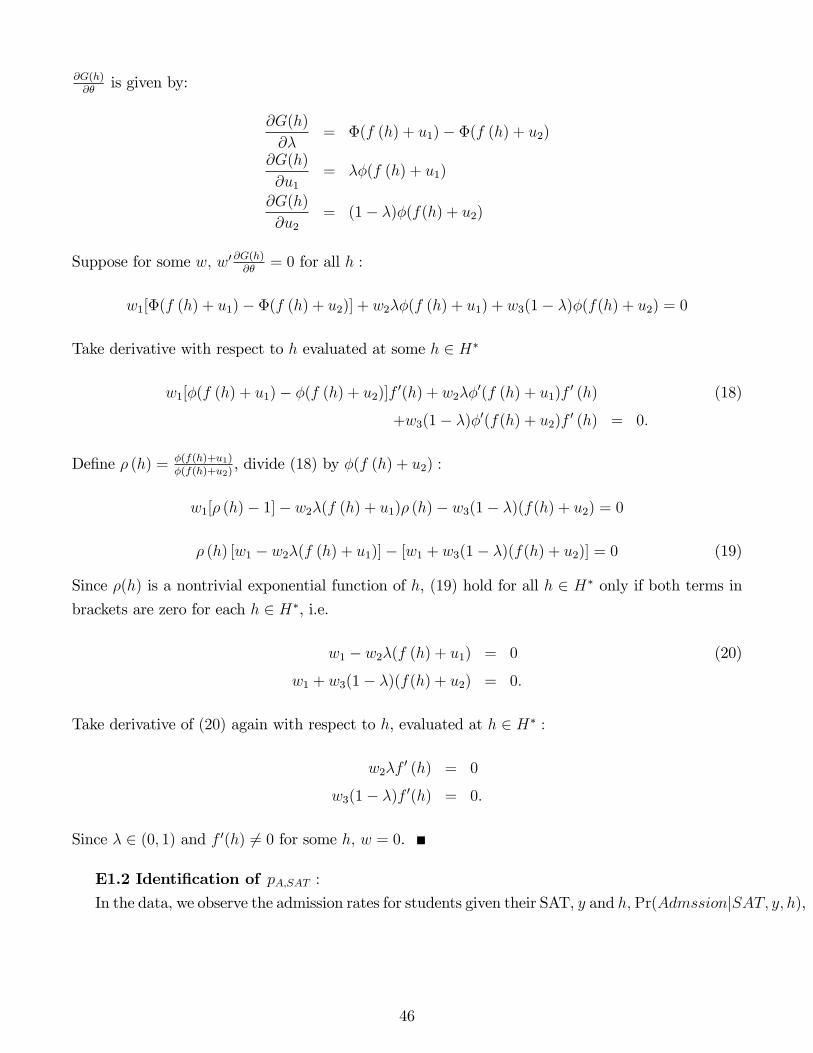
@G(h)@�

is given by:

@G(h)

@�= �(f (h) + u1)� �(f (h) + u2)

@G(h)

@u1= ��(f (h) + u1)

@G(h)

@u2= (1� �)�(f(h) + u2)

Suppose for some w; w0 @G(h)@�

= 0 for all h :

w1[�(f (h) + u1)� �(f (h) + u2)] + w2��(f (h) + u1) + w3(1� �)�(f(h) + u2) = 0

Take derivative with respect to h evaluated at some h 2 H�

w1[�(f (h) + u1)� �(f (h) + u2)]f 0(h) + w2��0(f (h) + u1)f 0 (h) (18)

+w3(1� �)�0(f(h) + u2)f 0 (h) = 0:

De�ne � (h) = �(f(h)+u1)�(f(h)+u2)

, divide (18) by �(f (h) + u2) :

w1[� (h)� 1]� w2�(f (h) + u1)� (h)� w3(1� �)(f(h) + u2) = 0

� (h) [w1 � w2�(f (h) + u1)]� [w1 + w3(1� �)(f(h) + u2)] = 0 (19)

Since �(h) is a nontrivial exponential function of h, (19) hold for all h 2 H� only if both terms in

brackets are zero for each h 2 H�, i.e.

w1 � w2�(f (h) + u1) = 0 (20)

w1 + w3(1� �)(f(h) + u2) = 0:

Take derivative of (20) again with respect to h, evaluated at h 2 H� :

w2�f0 (h) = 0

w3(1� �)f 0(h) = 0:

Since � 2 (0; 1) and f 0(h) 6= 0 for some h; w = 0.

E1.2 Identi�cation of pA;SAT :In the data, we observe the admission rates for students given their SAT, y and h; Pr(AdmssionjSAT; y; h),

46

which is generated via the following equation:

Pr(AdmssionjSAT; y; h) =

"� (SAT; y) p1;SAT Pr(applyjSAT; y; h; A = 1)

+ (1� � (SAT; y)) p2;SAT Pr(applyjSAT; y; h; A = 2)

#Pr(applyjSAT; y; h) : (21)

Given the identi�cation of � (SAT; y) and uA = u�A � cpA;SAT

as in E1.1, Pr(applyjSAT; y; h; A) =� (f(h; SAT; y) + uA) is also identi�ed. The denominator is directly from the data. De�ne the

following known objects

�(SAT; y; h; A = 1) =� (SAT; y) � (f(h; SAT; y) + u1)

Pr(applyjSAT; y; h) ;

�(SAT; y; h; A = 2) =(1� � (SAT; y)) � (f(h; SAT; y) + u2)

Pr(applyjSAT; y; h) :

Equation (21) can be written as

Pr(AdmssionjSAT; y; h) =XA

�(SAT; y; h; A) pA;SAT

The variations in y and/or h move both Pr(AdmssionjSAT; y; h) and �(SAT; y; h; A), which iden-ti�es pA;SAT for A = 1; 2:

E1.3 Identi�cation of u�A and cRecall that

uA;SAT = u�A �

c

pA;SAT:

Given that uA;SAT is identi�ed from E1.1 and pA;SAT from E1.2, �x A; both uA;SAT and pA;SAT vary

with SAT; which identi�es u�A and c:

E1.4 Relating the Identi�cation to the ModelIn practice, the variable y corresponds to family income (a 5-year average) and h other family

background variables. The identi�cation argument above assumes that 1) only SAT and family

income enter the type distribution, i.e., SAT and family (permanent) income summarize all in-

formation that correlates with ability; and 2) the expected �nancial aid depends on SAT and all

family-background variables. For example, conditional on family permanent income, family assets

(which serves the role of the h variable in the previous proof) vary with factors, such as housing

prices and stock prices, that are not correlated with ability.83

E2. Ability values ! :83This exclusion restriction is su¢ cient but not necessary for identi�cation. For example, I could allow family

assets to enter type distribution as a categorical variable, and to enter the �nancial aid function as a continuousvariable. The within-category variation in assets would be enough for identi�cation.

47

! is not point identi�ed, even after normalizing !1. The reasoning is as follows: each college

j faces discrete (s; SAT ) groups of applicants and its admissions policy depends on the rankings

of these groups in terms of their conditional expected abilities. These relative rankings remain

unchanged for a range of !�s, as do colleges�decisions and the model implications. Knowing that !

is not point identi�ed, I �x b! = [e; e2; e3]0. At other values of ! around [e; e2; e3]0, the estimates forthe other parameters in steps two and three will change accordingly. However, the counterfactual

experiment results are robust.84

F. Tuition ElasticityThis exercise examines students�responsiveness to tuition changes. A counterfactual experiment

based on the SPNE model is not directly comparable to previous studies because SPNE model en-

dogenizes tuition and admissions policies. Instead, I simulated the student decision model, holding

admissions probabilities at the baseline levels. In response to a $1; 000 (2003 dollars) tuition reduc-

tion, college enrollment will increase by 1%, which is lower than �ndings from previous studies.85

The discrepancy may be explained by the di¤erent cohorts of students studied in various papers.

This paper studies a cohort of students who enter college around 2002, much younger than those

studied in previous literature. As shown in Figures 2 and 3, which are based on data from National

Center for Education Statistics, state and local government spending on higher education has been

rising over time, suggesting some expansion on the supply side. Such a pattern was accompanied by

steady growth in college enrollment rate in earlier years. However, college attendance has been stag-

nant since 1998. These �gures are consistent with the hypothesis that a lower fraction of students

in the later cohorts are at the margin.86

G. Additional TablesG1. Parameter Estimates

Table G1.1 Ordered Logit Ability Distribution

cut1 cut2 y=1000 (y=1000)2 SAT= 2 SAT= 3

2:56 6:38 0:02 �0:00003 3:72 5:02

(0:21) (0:37) (0:005) (0:00002) (0:24) (0:36)

cut1; cut2 are the cuto¤ parameters for the ordered logit.

84Results available upon request.85For example, Leslie and Brinkman (1998) and Cameron and Heckman (2001).86Although di¤erent, this hypothesis is not in con�ict with Lochner and Monge-Naranjo (2011). In this hypothesis,

there are more students from the later cohorts that are constrained, but instead of at college age, in their childhoodwhen their pre-college human capital is formed. By college age, these "long-term-constrained" students are not atthe margin and therefore are not easily attracted to colleges by moderate tuition reductions.

48

Table G1.2 Z Type Distribution By Ability

A = 1 A = 2 A = 3

Pr (z = 1jA) 1:0 0:75 0:70

- (0:04) (0:05)a Pr(z= 1jA = 1) = 1 cannot be rejected at 10% signi�cance level.b 86% of all students are of z-1 type.

Table G1.3 Ability Distribution

% A = 1 A = 2 A = 3

All 48:6 38:8 13:2

z= 1 55:6 33:7 10:7

z= 2 0:0 71:0 29:0

Simulation based on the estimates in Tables G1.1 and G1.2.

Ability distribution among all students and by z type.

Table G1.4 Ability, SAT and Signals Among Applicants

A = 1 A = 2 A = 3

% Applicants 3:5 68:5 28:0

SAT = 1 SAT = 2 SAT = 3

% Applicants 15:4 60:4 24:2

s = 1 s = 2 s = 3

% Applicants 8:6 73:2 18:2

Simulation based on the estimates in Tables G1.1 and G1.2.

Distribution among all applicants: each row adds up to 100%.

49

Table G1.5 Financial Aid

General aid College-Speci�c Aid

Coe¢ cient Std. Error Coe¢ cient Std. Error

Constant �6087:6 (848:2) �12641:8 (2297:5)

Black 921:6 (927:5) 6774:1 (1819:9)

Family Income/1000 �34:7 (10:7) �71:6 (16:5)

Family Assets/1000 �4:4 (2:5) �5:9 (4:8)

SAT= 2 2334:4 (987:8) 3747:9 (2250:9)

SAT= 3 4366:2 (1240:8) 7342:0 (2498:1)

Sibling in Collegea 944:6 (832:1) 2958:2 (1751:9)

(SAT= 2)� private 12169:7 (1802:3)

(SAT= 3)� private 15130:8 (2391:4)

4-Yr Colleges 4123:0 (960:6)

(pri,elite) �11764:6 (4845:9)

2-Yr Colleges �4281:5 (2077:3)

�� (aid shock) 498:0 (210:4) 6796:6 (193:6)

�err (measurement) 7047:3 (1284:0) 10466:0 (612:3)

a: Whether the student has some siblings in college at the time of application.

Table G1.6 Capacities (%)

�1 �2 �3 �4

1:1 (0:1) 8:2 (0:2) 10:8 (0:03) 20:0 (0:07)

Table G1.7 Tuition Weights

(pri,elite) (pub,elite) (pri,non) (pub,non)

In-State Out-of-State In-State Out-of-State

m2j �0:0012 �0:0069 �0:0004 �0:0012 �0:0085 �0:0015(0:0002) (0:002) (0:0001) (0:003) (0:0009)

m1j 0:0701 (0:002)

Tuition is measured in thousands of dollars. m1j are restricted to be the same across j�s.

Allowing m2j to di¤er between the two private college groups does not improve the �t.

G2. Model Fit

50

Table G2.1.1 Num. of Applications: by SAT

% SAT=1� SAT=2 SAT=3�

n Data Model Data Model Data Model

0 85:1 86:3 24:9 24:4 13:0 12:4

1 12:1 8:3 45:2 44:1 43:0 57:6

2 or more 2:8 5:4 29:9 31:5 44:0 30:0��2 > �22;0:05

Table G2.1.2 Num. of Applications: by Family Inc

% Income < Median� Income � Median

n Data Model Data Model

0 68:2 68:4 40:2 40:5

1 22:1 19:0 33:9 36:5

2 or more 9:7 12:6 25:9 22:9��2 > �22;0:05

Table G2.2.2 Application Rates: by Family Inc

% Income < Median Income � Median

Data Model Data Model

(pri,elite) 7:6 5:8 10:8 11:4

(pub,elite) 21:8 20:8 37:2 32:6

(pri,non) 39:7 40:6 47:2 51:5

(pub,non) 76:0 72:3 69:1 65:1

Table G2.3.1 Admission Rates: by SAT

% SAT=1 SAT=2 SAT=3

Data Model Data Model Data Model

(pri,elite) n=a 22:1 38:5 41:3 61:7 76:2

(pub,elite) 53:8 16:0� 80:0 91:0 92:8 98:0

(pri,non) 83:9 77:1 93:0 93:7 94:0 100:0

(pub,non) 83:9 83:1 95:0 98:5 99:0 100:0� �2 > �21;0:05

51

Table G2.3.2 Admission Rates: by Family Inc

% Income < Median Income � Median

Data Model Data Model

(pri,elite) 55:0 51:1 52:8 60:6

(pub,elite) 91:2 86:9 80:3 92:6�

(pri,non) 86:5 87:8 93:5 92:9

(pub,non) 91:0 93:7 95:6 97:2� �2 > �21;0:05

Table G2.4.1 Final Allocation: by SAT

% SAT=1 SAT=2� SAT=3

Data Model Data Model Data Model

(pri,elite) 0:0 0:1 0:2 1:8 7:3 6:7

(pub,elite) 0:4 0:2 13:0 13:0 22:2 25:8

(pri,non) 4:3 3:4 16:9 18:7 25:6 18:2

(pub,non) 6:9 6:3 39:7 35:2 31:0 32:2

2-yr college 25:8 27:0 22:4 20:7 11:1 13:8

Outside 62:6 63:1 7:9 10:5 2:9 3:3� �2 > �25;0:05

Table G2.4.2 Final Allocation: by Family Inc

% Income < Median Income � Median�

Data Model Data Model

(pri,elite) 0:6 0:6 1:3 2:5

(pub,elite) 3:9 3:5 11:5 12:5

(pri,non) 7:2 8:5 15:9 13:2

(pub,non) 15:8 14:4 28:0 25:8

2-yr college 22:7 25:0 22:7 21:1

Outside 49:8 48:0 20:5 24:9� �2 > �25;0:05

Table G2.5.1 Home Bias: by SAT

SAT=1 SAT=2 SAT=3

(%) Data Model Data Model Data Model

Home-Only Applicantsa 79:2 63:8� 68:0 68:6 50:3 62:6�

Home-State Attendeesb 85:6 78:8 78:7 79:1 65:2 74:8� �2 > �21;0:05a % students who apply only within home states among all 4-yr applicants.b % students who attend home-state 4-yr colleges among all 4-yr attendees.

52

Table G2.5.2 Home Bias: by Family Inc

Income < Median Income � Median

(%) Data Model Data Model

Home-Only Applicants 72:1 67:5 62:2 67:5

Home-State Attendees 80:5 79:1 74:1 77:4

53

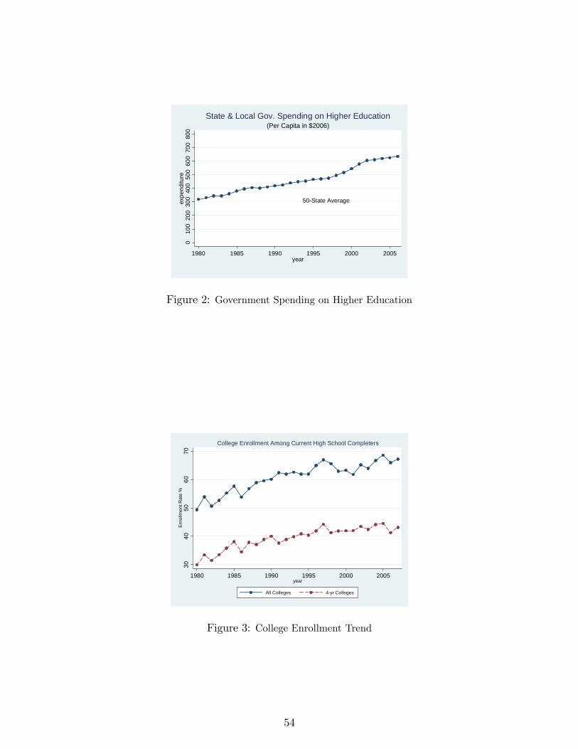
010

020

030

040

050

060

070

080

0ex

pend

iture

1980 1985 1990 1995 2000 2005year

50­State Average

(Per Capita in $2006)State & Local Gov. Spending on Higher Education

Figure 2: Government Spending on Higher Education

3040

5060

70En

rollm

ent R

ate 

%

1980 1985 1990 1995 2000 2005year

All Colleges 4­yr Colleges

College Enrollment Among Current High School Completers

Figure 3: College Enrollment Trend

54