European Journal of Operational Research 237 (2014) 957–965

Contents lists available at ScienceDirect

European Journal of Operational Research

journal homepage: www.elsevier .com/locate /e jor

Decision Support

Equilibrium in an ambiguity-averse mean–variance investors market q

http://dx.doi.org/10.1016/j.ejor.2014.02.0160377-2217/� 2014 Elsevier B.V. All rights reserved.

q Revision: December 2013.⇑ Tel.: +90 3122902603.

E-mail address: mustafap@bilkent.edu.tr

Mustafa Ç. Pınar ⇑Department of Industrial Engineering, Bilkent University, 06800 Bilkent, Ankara, Turkey

a r t i c l e i n f o a b s t r a c t

Article history:Received 2 July 2013Accepted 5 February 2014Available online 12 February 2014

Keywords:Robust optimizationMean–variance portfolio theoryEllipsoidal uncertaintyEquilibrium price system

In a financial market composed of n risky assets and a riskless asset, where short sales are allowed andmean–variance investors can be ambiguity averse, i.e., diffident about mean return estimates where con-fidence is represented using ellipsoidal uncertainty sets, we derive a closed form portfolio rule based on aworst case max–min criterion. Then, in a market where all investors are ambiguity-averse mean–vari-ance investors with access to given mean return and variance–covariance estimates, we investigate con-ditions regarding the existence of an equilibrium price system and give an explicit formula for theequilibrium prices. In addition to the usual equilibrium properties that continue to hold in our case,we show that the diffidence of investors in a homogeneously diffident (with bounded diffidence)mean–variance investors’ market has a deflationary effect on equilibrium prices with respect to a puremean–variance investors’ market in equilibrium. Deflationary pressure on prices may also occur if oneof the investors (in an ambiguity-neutral market) with no initial short position decides to adopt an ambi-guity-averse attitude. We also establish a CAPM-like property that reduces to the classical CAPM in caseall investors are ambiguity-neutral.

� 2014 Elsevier B.V. All rights reserved.

1. Introduction and background

A major theme in mathematical finance is the study of inves-tors’ portfolio decisions using the well-established theory ofmean–variance that began with the seminal work of Markowitz(1987). The mean–variance portfolio theory then formed the basisof the celebrated Capital Asset Pricing Model (CAPM) (Sharpe,1964), the most commonly used equilibrium and pricing modelin the financial literature. However, it is a well-known fact thatthe investors’ portfolio holdings in the mean–variance portfoliotheory are very sensitive to the estimated mean returns of the riskyassets; see e.g., Best and Grauer (1991a), Best and Grauer (1991b),Black and Litterman (1992). The purpose of the present paper is toinvestigate equilibrium relations in a financial market composed ofn risky assets and a riskless asset using an approach that takes intoaccount the imprecision in the mean return estimates. In our mod-el, investors act as mean–variance investors with a degree of diffi-dence (or confidence) towards the mean return estimates of riskyassets. We refer to this attitude of diffidence as ambiguity aversionto distinguish it from risk aversion quantified by a mean–varianceobjective function. Decision making under ambiguity aversion is anactive research area in decision theory and economics; see e.g.,

Klibanoff, Marinacci, and Mukerji (2005, 2009). Our study followsthe earlier work of Konno and Shirakawa (1994, 1995), and is inparticular inspired by the previous work of Deng, Li, and Wang(2005) where the authors study a similar problem allowing themean returns of risky assets to vary over a hyper-rectangle, i.e.,an interval is specified for each mean return estimate and amax–min approach is used in the portfolio choice as in the presentpaper. We adopt an ellipsoidal uncertainty set for the mean-returnvector instead of a hyper-rectangle, and obtain a closed-form port-folio rule using a worst-case max–min approach as in the robustoptimization framework of Ben-Tal and Nemirovski (1999, 1998).In contrast, in Deng et al. (2005) a closed-form portfolio rule isnot possible due to the polyhedral nature of their ambiguity repre-sentation. The ellipsoidal model controls the diffidence of investorsusing a single positive parameter � while the interval model ofDeng et al. (2005) requires the specification of an interval for eachrisky asset, and has to resort to numerical solution of a linear pro-gramming problem to find a worst-case rate of return vector in thehyper-rectangle. The linear programming nature of the proceduremay cause several components of the rate of return vector in ques-tion to assume the lower or upper end values of the interval as aby-product of the simplex method (i.e., an extreme point of the hy-per-rectangle will be found). Since the worst case return occurs atan extreme point of the hyper-rectangle, it corresponds to an ex-treme scenario where most (or all) risky assets assume their worstpossible return values, which may translate into an unnecessarily

958 M.Ç. Pınar / European Journal of Operational Research 237 (2014) 957–965

conservative portfolio. Such extreme behavior does not occur withan ellipsoidal representation of the uncertainty set due to the non-linear geometry of the ellipsoid. Besides, the ellipsoidal representa-tion is also motivated by statistical considerations alluded to inSection 2. As in Deng et al. (2005), in the contributions of Konnoand Shirakawa (1994, 1995) where short sales are not allowed,the formula for the equilibrium price vector requires the solutionof an optimization problem as input to the formula whereas wehave an explicit formula for the equilibrium price.

To the best of our knowledge, the present paper is one the fewstudies next to Deng et al. (2005), Wu, Song, Xu, and Liu (2009) toincorporate ambiguity aversion in asset returns in an equilibriumframework. However, unlike the present paper, in neither Denget al. (2005) nor Wu et al. (2009) there is a truly closed-form result,and furthermore they do not study the impact of ambiguity aver-sion on equilibrium prices.

The seminal results on equilibrium in capital markets wereestablished in the early works of Lintner (1965), Mossin (1966)and Sharpe (1964), which resulted in the celebrated CAPM; see El-ton and Gruber (1991), Markowitz (1987) for textbook treatmentsof the subject. The theory of equilibrium in capital asset marketswere later extended in several directions in e.g., Black (1972), Niel-sen (1987, 1989, 1990, 1989). In a recent study, Rockafellar, Urya-sev, and Zabarankin (2007) use the so-called diversion measures (anexample is Conditional Value at Risk, CVaR) to investigate equilib-rium in capital markets. Balbás, Balbás, and Balbás (2010) usecoherent risk measures, expectation bounded risk measures andgeneral deviations in optimal portfolio problems, and studyCAPM-like relations. Grechuk and Zabarankin (2012) consider anoptimal risk sharing problem among agents with utility functionalsdepending only on the expected value and a deviation measure ofan uncertain payoff. They characterize Pareto optimal solutionsand study the existence of an equilibrium. Kalinchenko, Uryasev,and Rockafellar (2012) use the generalized CAPM based on mixedConditional Value at Risk deviation for calibrating the risk prefer-ences of investors. Hasuike (2010) use fuzzy numbers to representinvestors’ preferences in an extension of the CAPM. Zabarankin,Pavlikov, and Uryasev (2014) uses the Conditional Drawdown-at-Risk (CDaR) measure to study optimal portfolio selection andCAPM-like equilibrium models. Won and Yannelis (2011) examineequilibrium with an application to financial markets without ariskless asset where uncertainty makes preferences incomplete.They assume a normal distribution for the mean return with anuncertain mean, and adopt a min–max approach using an ellipsoi-dal representation as in the present paper.

In the present paper, we investigate the equilibrium implica-tions of ambiguity aversion defined as diffidence vis à vis esti-mated mean returns. In particular, in a capital market inequilibrium where all investors fully trust estimated mean ratesof return (they are ambiguity-neutral), if one investor decides toadopt an ambiguity-averse position, this shift may create a down-ward pressure on equilibrium prices. In uniform markets where allinvestors are ambiguity averse, the effect of ambiguity aversion isalso deflationary with respect to a fully confident (ambiguity-neu-tral) investors market.

In summary, the contributions of the present are as follows:

� we use an ellipsoidal representation of the ambiguity in meanreturns which avoids extreme scenarios, and thus alleviatesthe overly conservative nature of the resulting portfolios,� our ellipsoidal ambiguity model allows for a truly closed-form

portfolio rule,� we establish a sufficient condition for a unique equilibrium

price vector in financial markets with ambiguity averse inves-tors, as well as a necessary and sufficient condition for existenceof non-negative equilibrium prices,

� we have an explicit formula for the equilibrium price system ina market of mean–variance and ambiguity-averse investors,which reduces to a formula for the equilibrium prices of a mar-ket of mean–variance investors,� we show the deflationary effect of the ambiguity aversion on

risky asset prices,� we establish a generalization of the CAPM which reverts to the

original CAPM when all investors are ambiguity-neutral.

The paper is organized as follows. In Section 2 we examine theproblem of portfolio choice of an ambiguity-averse investor usingan ellipsoidal ambiguity set and worst case max–min criterion.We derive an explicit optimal portfolio rule. In Section 3, we studyconditions under which an equilibrium system of prices exist indifferent capital markets characterized by the presence of ambigu-ity-averse or neutral investors, and give an explicit formula forequilibrium prices. We illustrate the results with a numericalexample. Section 4 gives some properties of equilibrium. In partic-ular, separation and proportion properties are shown, as well as aCAPM-like result which reduces to the classical CAPM when inves-tors have full confidence in the estimates of mean rate of return.We conclude in Section 5 with a summary and future researchdirections.

2. Ambiguity-averse mean–variance investor’s portfolio rule

Let the price per share of asset j be denoted pj, j ¼ 1;2; . . . ;n forthe first n risky assets in the market, we assume the price of thenþ 1th riskless asset to be equal to one. We denote by x0

j the num-ber of shares of asset j held initially by the investor while we use xj

to denote the number of shares of asset j held by the investor afterthe transaction, for all j ¼ 1; . . . ;nþ 1. Unlimited short positionsare allowed, i.e., there is no sign restriction on xj.

The n risky assets have random rate of return vectorr ¼ ðr1; r2; . . . ; rnÞ and estimate of mean rate of return vectorr̂ ¼ ðr̂1; r̂2; . . . ; r̂nÞ (that we shall also refer to as the nominal rateof return) with variance–covariance matrix estimate C which is as-sumed positive definite. The ðnþ 1Þth position is reserved for theriskless asset with deterministic rate of return equal to R. Theinvestor has a risk aversion coefficient x 2 ð0;1Þ and an initialendowment W0 assumed positive such that

W0 ¼Xn

j¼1

pjx0j þ x0

nþ1:

Since there are no withdrawals from and injections to the port-folio, we still have, after the transaction,

W0 ¼Xn

j¼1

pjxj þ xnþ1:

Dividing the last equation by W0 and defining the proportionsyj �

pjxj

W0for j ¼ 1; . . . ;nþ 1 we have that

Xnþ1

j¼1

yj ¼ 1:

If we denote the true (unknown) mean rates of return by rj forj ¼ 1; . . . ;n the mean rate of return of portfolio x (with proportionsyj) is equal to

Xn

j¼1

rjyj þ Rynþ1

with variance equal toPn

j¼1

Pnk¼1Cjkyjyk ¼ yTCy where y denotes the

vector with components ðy1; . . . ; ynÞ. Note that the random end-of-period wealth W1 is given as

M.Ç. Pınar / European Journal of Operational Research 237 (2014) 957–965 959

W1 ¼W0

Xn

i¼1

riyi þ Rynþ1

" #:

The investor is also ambiguity averse with ambiguity aversioncoefficient � such that his/her confidence in the mean rate of returnvector estimate is expressed as a belief that the true mean rate ofreturn lies in the ellipsoidal set

Ur ¼ frjkC�1=2ðr� r̂Þk2 6 �g;

that is, an n-dimensional ellipsoid centered at r̂ (the estimatedmean return vector) with radius �. The idea is that the decisionsof an ambiguity averse investor are made by considering the worstcase occurrences of the true mean rate of return r within the setUr . Therefore, more conservative portfolio choices are made whenthe volume of the ellipsoid is larger, i.e. for greater values of �,while an ambiguity-neutral investor with no doubt about errorsin the estimated values sets � equal to zero. The differences be-tween the true mean rate of return r and its forecast r̂ dependon the variance of the returns, hence they are scaled by the inverseof the covariance matrix. To quote Fabozzi, Kolm, Pachamanova,and Focardi (2007): ‘‘The parameter � corresponds to the overallamount of scaled deviations of the realized returns from theforecasts against which the investor would like to be protected’’.Garlappi, Uppal, and Wang (2007) show that the ellipsoidal repre-sentation of the ambiguity of estimates may also lead to morestable portfolio strategies, delivering a higher out-of-sampleSharpe ratio compared to the classical Markowitz portfolios. It isalso well-known (see Johnson & Wichern (1997, p. 212)), thatthe random variable

ðr� r̂ÞTC�1ðr� r̂Þ;

has a known distribution (F-distribution under standard assump-tions on the time series of returns), and this fact can be exploitedusing a quantile framework to set meaningful values for � in prac-tical computation with return data, c.f. Garlappi et al. (2007).

The ambiguity-averse mean–variance investor is interested inchoosing his/her optimal portfolio according to the solution ofthe following problem

maxy

minr2Urð1�xÞðrT y þ ð1� eT yÞRÞ �xyTCy

where e represents an n-vector of ones and the scalar x 2 ð0;1Þ rep-resents the degree of risk aversion of the investor. The larger the va-lue of x, the more risk averse (in the sense of aversion to variance ofportfolio return) the investor. Processing the inner min we obtain asusual the problem:

maxyð1�xÞðr̂T y þ ð1� eT yÞR� �kC1=2yk2Þ �xyTCy

that is referred to as AAMVP (abbreviation of Ambiguity AverseMean–Variance Portfolio). Let l̂ ¼ r̂ � Re. Hence we can re-writeAAMVP as

maxyð1�xÞðl̂T y þ R� �kC1=2yk2Þ �xyTCy:

Let us define the market optimal Sharpe ratio as H2 ¼ l̂TC�1l̂.

Proposition 1. If � < H then AAMVP admits the unique optimalsolution

y� ¼ 1�x2x

� �H � �

H

� �C�1l̂; y�nþ1

¼ 1�Xn

j¼1

1�x2x

� �H � �

H

� �ðC�1l̂Þj

i.e., an ambiguity-averse mean–variance investor with limited diffi-dence (� < H) makes the optimal portfolio choice in the risky assets

x�j ¼W0

pj

!1�x

2x

� �H � �

H

� �ðC�1l̂Þj; j ¼ 1; . . . ;n:

If �P H, then it is optimal for an AAMVP investor to keep all initialwealth in the riskless asset.

Proof. The function is strictly concave. The first-order necessaryand sufficient conditions (assuming a solution y–0) yields the can-didate solution:

y� ¼ ð1�xÞrð1�xÞ�þ 2rx

� �C�1l̂;

where we defined r �ffiffiffiffiffiffiffiffiffiffiffiffiyTCy

p. Using the definition of r we obtain

ð1�xÞ2H2 ¼ ðð1�xÞ�þ 2rxÞ2. Developing the parentheses onthe right side we obtain a quadratic equation in r

4x2r2 þ 4xð1�xÞ�rþ ð1�xÞ2ð�2 � H2Þ ¼ 0

with the positive root rþ ¼ ð1�xÞðH��Þ2x provided that � < H. Then the

result follows by simple algebra. If �P H then our supposition thata non-zero solution exists has been falsified, in which case we re-vert to the origin as the optimal solution. h

Notice that when the investor is not ambiguity averse, i.e.,� ¼ 0, one recovers the optimal portfolio rule of a mean–varianceinvestor, namely,

y� ¼ 1�x2x

� �C�1l̂:

The factor H��H < 1 in the optimal portfolio of a diffident investor

whose diffidence is bounded above by the slope of the Capital Mar-ket Line (we shall refer to such investors as mildly diffident, we shallalso be using the terms bounded diffidence or limited diffidence inthe same context), tends to curtail both long and short positionswith respect to the portfolio of a fully confident (i.e., ambiguity-neutral) investor.

An alternative proof would proceed by exchanging the max andthe min as in Deng et al. (2005). Solving the max problem first forfixed r, one finds the point

y ¼ 1�x2x

C�1ðr� ReÞ: ð1Þ

Then minimizing the resulting maximum

ð1�xÞRþ ð1�xÞ2

4xðr� ReÞTC�1ðr� ReÞ

over the set Ur one finds the worst case rate of return r� as the uniqueminimizer of the above function (this is missing in the analysis ofDeng et al. (2005)):

r� ¼ H � �H

r̂ þ �RH

e; ð2Þ

which when plugged into (1) for r results in the solution we haveobtained in Proposition 1.

3. Existence of an equilibrium price system

In this section we shall analyze the existence of an equilibriumprice system in capital markets where investors adopt or relin-quish an ambiguity-averse attitude. First, we shall look at marketswhere all investors are either ambiguity-averse or ambiguity-neu-tral. We refer to such markets as uniform markets. Then, we inves-tigate the effect on equilibrium prices of introducing an ambiguity-averse investor in a market of ambiguity-neutral investors. Weshall refer to such markets as mixed.

960 M.Ç. Pınar / European Journal of Operational Research 237 (2014) 957–965

We denote the price system by the vector ðp1; p2; . . . ; pnÞ for then risky assets. The price of the riskless asset is assumed to be equalto one. We make the following assumptions:

1. The total number of shares of asset j is x0j , j ¼ 1;2; . . . ;nþ 1.

2. Investors i ¼ 1; . . . ;m make their static portfolio choicesaccording to the ambiguity-averse mean–variance portfoliomodel AAMVP of the previous section; they all agree onthe nominal excess return vector l̂ (i.e., they all agree onthe same nominal rate of return vector r̂ and the sameriskless rate R) and positive-definite variance–covariancematrix C.

3. Investor i invests an initial wealth W0i in an initial portfolio

x0i1; x

0i2; . . . ; x0

inþ1

� �.

4. Investor i has risk aversion coefficient xi and ambiguity aver-sion coefficient (diffidence level) �i.

We have

Xm

i¼1

x0ij ¼ x0

j ; j ¼ 1;2; . . . ;nþ 1; ð3Þ

Xn

j¼1

pjx0ij þ x0

inþ1 ¼W0i : ð4Þ

�1 �1 �1 T �1

3.1. Uniform markets

Using the result from the previous section we have that eachinvestor i holds the percentage portfolio

y�ij ¼1�xi

2xi

H � �i

HðC�1l̂Þj; j ¼ 1;2; . . . ;n; ð5Þ

y�inþ1 ¼ 1�Xn

j¼1

y�ij ¼ 1� 1�xi

2xi

H � �i

H

Xn

j¼1

ðC�1l̂Þj ð6Þ

under the assumption that each investor i operates under limiteddiffidence, i.e., �i < H; i ¼ 1; . . . ;m. Passing to the corresponding as-set portfolio holdings (shares) x�ij we have

x�ij ¼W0

i y�ijpj¼W0

i

pj

1�xi

2xi

H � �i

HðC�1l̂Þj; j ¼ 1;2; . . . ;n; ð7Þ

x�inþ1 ¼W0i y�inþ1 ¼W0

i 1�Xn

j¼1

y�ij

!¼W0

i 1� 1�xi

2xi

H � �i

H

Xn

j¼1

ðC�1l̂Þj

!: ð8Þ

The market clearing condition requires the following equationto hold:

Xm

i¼1

x�ij ¼ x0j ; j ¼ 1;2; . . . ;nþ 1; ð9Þ

i.e., we have

Xm

i¼1

W0i

pj

1�xi

2xi

H � �i

HðC�1l̂Þj ¼ x0

j ; j ¼ 1;2; . . . ;nþ 1; ð10Þ

Re-arranging this equation and recalling (4) we have the equationsystem with n equations and n unknowns:

pjx0j ¼ ðC

�1l̂ÞjXm

i¼1

1�xi

2xi

� �H � �i

H

� � Xn

k¼1

pkx0ik þ x0

inþ1

!;

j ¼ 1;2; . . . ;n: ð11Þ

Now, define for convenience fj ¼ ðC�1l̂Þj for j ¼ 1;2; . . . ;nand

a ¼Xm

i¼1

Xn

j¼1

1�xi

2xi

� �H � �i

H

� � x0ij

x0j

fj:

Proposition 2. In an ambiguity-averse mean–variance investors’market where every investor has limited diffidence (i.e., �i < H forall i ¼ 1; . . . ;m) if a–1, then there exists a unique solution p� to theequilibrium system (11) given by

p�j ¼1

1� afj

x0j

Xm

i¼1

1�xi

2xi

� �H � �i

H

� �x0

inþ1; j ¼ 1; . . . ;n: ð12Þ

IfPm

i¼11�xi2xi

� �H��i

H

� �x0

ij P 0; j ¼ 1;2; . . . ;nþ 1, and no investor is

short on risky assets, i.e., fj P 0 for all j ¼ 1; . . . ;n, then the marketadmits a unique non-negative equilibrium price vector p� if and only

if a < 1.

Proof. The proof is almost identical to the proof of Theorem 4.1 inDeng et al. (2005) with minor modifications. Let

cj ¼Xm

i¼1

1�xi

2xi

� �H � �i

H

� �x0

ij; j ¼ 1;2; . . . ;nþ 1;

and

dj ¼ fj=x0j ; ;j ¼ 1;2; . . . ;n:

Let c be the vector with components ðc1; . . . ; cnÞ and d the vectorwith components ðd1; . . . ; dnÞ. Then we can express a as a ¼ cT d.The system (11) can now be re-written as

pj ¼fj

x0j

Xm

i¼1

1�xi

2xi

� �H � �i

H

� �Xn

k¼1

pkx0ik þ

fj

x0j

Xm

i¼1

1�xi

2xi

� �H � �i

H

� �x0

inþ1

¼ dj

Xn

k¼1

pk

Xm

i¼1

1�xi

2xi

� �H � �i

H

� �x0

ik þ djcnþ1

¼Xn

k¼1

ckpk þ djcnþ1; j ¼ 1;2; . . . ;n:

In vector form we have the equation

p ¼ dðcT pÞ þ cnþ1d;

or, equivalently

ðI � dcTÞp ¼ cnþ1d:

Then, when a–1 the system has the unique solution

p ¼ cnþ1ðI � dcTÞ�1

d ¼ cnþ1 I þ dcT

1� a

!d ¼ cnþ1

1� ad; ð13Þ

where the second equality follows from the Sherman–Morrison–Woodbury formula.1 The rest of the proof consists of applying FarkasLemma (c.f. chapter 2 of Mangasarian (1994)) to the system

ðI � dcTÞp ¼ cnþ1d; p P 0;

and its alternative

ðI � cdTÞy 6 0; dT y > 0;

under the conditions c P 0; fj P 0 for all j ¼ 1; . . . ;n and a < 1. Ifa < 1, then the unique solution in (13) is non-negative. If a P 1,then y ¼ c satisfies the alternative system, hence no non-negativeequilibrium prices exist. h

The scalar a plays an important role in the existence of equilib-rium results (see also Deng et al. (2005), Konno & Shirakawa (1995)and the scalar c in Corollary 1 below). However, a financial inter-pretation of the condition involving a is missing from the litera-ture. Note that the double summation in a, considered without

1 ðAþ uvT Þ ¼ A � A uv A1þvT A�1u

.

M.Ç. Pınar / European Journal of Operational Research 237 (2014) 957–965 961

the ratio termx0

ij

x0j

(which represents the investor i’s initial fraction of

shares of asset j) would give the total of fraction portfolio holdings(y�ij) in the market, summed over all investors and all risky assets.Thus, the scalar a gives a measure of the weighted total of fractionportfolio holdings where each y�ij is weighted by the corresponding

ratiox0

ij

x0j. If this weighted total is strictly less than 1, an equilibrium

price exists as is shown in the proposition above. The condition isalso necessary. The condition

Xm

i¼1

1�xi

2xi

� �H � �i

H

� �x0

ij P 0; j ¼ 1;2; . . . ;nþ 1

also represents a weighted total of initial portfolio holdings over all

investors in the market. The weight 1�xi2xi

� �H��i

H

� �encodes the risk

aversion and ambiguity aversion attitudes of the investor.The existence of strictly positive prices is a harder question that

is rarely addressed (with the exception of Rockafellar et al. (2007))although zero prices would hardly make economic sense in prac-tice. Interestingly, we can also prove the following negative resulton the existence of a strictly positive system of equilibrium prices.

If the condition of Proposition 2Pm

i¼11�xi2xi

� �H��i

H

� �x0

ij P 0; j ¼ 1;

2; . . . ;n partially holds (only for the risky assets), i.e., a weightedtotal of initial portfolio holdings of risky assets over all investorsin the market is non-negative, while this total is negative for theriskless asset then it is not possible to have positive equilibriumprices in the market.

Proposition 3. IfPm

i¼11�xi2xi

� �H��i

H

� �x0

ij P 0; j ¼ 1;2; . . . ;n; cnþ1 < 0,

no investor is short on risky assets, i.e., fj P 0 for all j ¼ 1; . . . ;n, anda 2 ð0;1Þ then a strictly positive equilibrium price system does notexist in an ambiguity-averse mean–variance investors’ market whereevery investor has limited diffidence (i.e., �i < H for all i ¼ 1; . . . ;m).

Proof. We shall invoke the non-homogeneous Stiemke theorem(Stiemke, 1915) for the system:

ðI � dcTÞp ¼ cnþ1d; p > 0;

The alternative of the above system according to Stiemke’s theo-rem2 is the system

I � cdT

�cnþ1d

!x P 0;

I � cdT

�cnþ1d

!x – 0;

If x ¼ c then

I � cdT

�cnþ1d

� �x ¼ cð1� aÞ

�cnþ1a

� �:

Since by assumption we havePm

i¼11�xi2xi

� �H��i

H

� �x0

ij P

0; j ¼ 1;2; . . . ;n, we have c P 0. Due to the hypotheses thata 2 ð0;1Þ and cnþ1 < 0 we have x ¼ c that satisfies the alternativesystem. h

If the market consists of fully confident (in the mean rate ofreturn estimates) investors (i.e., ambiguity-neutral), we have thefollowing equilibrium result in a mean–variance capital market.Let us define for convenience

c ¼Xm

i¼1

Xn

j¼1

1�xi

2xi

� � x0ij

x0j

fj:

2 Stiemke’s Theorem: Either AT y ¼ b; y > 0 has a solution or Ax P 0;�bT x P 0;Ax�bT x

� �– 0 has a solution, but never both, c.f. Chapter 6 of Panik (1993).

Corollary 1. In a mean–variance investors’ market (with no ambi-guity aversion) if c–1, then there exists a unique solution p� to theequilibrium system (11) given by

pmvj ¼ 1

1� cfj

x0j

Xm

i¼1

1�xi

2xi

� �x0

inþ1; j ¼ 1; . . . ;n: ð14Þ

IfPm

i¼11�xi2xi

� �x0

ij P 0; j ¼ 1;2; . . . ;nþ 1, and fj P 0 for all

j ¼ 1; . . . ;n, then the market admits a unique non-negative equilib-

rium price vector p� if and only if c < 1.As in Proposition 2 the scalar c gives a measure of the weighted

total of fraction portfolio holdings where each y�ij is weighted by

the corresponding ratiox0

ij

x0j.

An interesting case is when all ambiguity-averse investors agreeon the same level of limited diffidence, i.e., �i ¼ � < H for alli ¼ 1; . . . ;m. In that case, the equilibrium price vector p� has a sim-plified expression:

pHj ¼

H � �Hð1� aÞ

fj

x0j

Xm

i¼1

1�xi

2xi

� �x0

inþ1; j ¼ 1; . . . ;n: ð15Þ

Obviously, the above expression implies pHj ¼

ðH��Þð1�cÞH�ðH��Þc pmv

j . Now,since we have

0 <ðH � �Þð1� cÞH � ðH � �Þc ¼

H � Hcþ �c� �H � Hcþ �c < 1

as c < 1 in equilibrium, and H > � > 0. Therefore, in a homoge-neously and mildly diffident ambiguity-averse mean–varianceinvestors’ market (where diffidence is bounded above by the slopeof the Capital Market Line), equilibrium prices are under downwardpressure with respect to a purely confident mean–variance inves-tors’ market. We summarize these observations below.

Proposition 4. In a homogeneously and mildly diffident (where allinvestors have the same � < H) ambiguity-averse mean–varianceinvestors’ market in equilibrium prices are smaller than the equilib-rium prices in a pure mean–variance investors’ market.

Another interesting observation is the following. Assume noinvestor has an initial liability, i.e., x0

ij > 0 for all i ¼ 1; . . . ;m andfj > 0 for all j ¼ 1; . . . ;n. Then we have the immediate conse-quence that a < c. This implies straightforwardly that p�j < pmv

j ,for all j ¼ 1; . . . ;n. In other words, in an ambiguity-averse mean–var-iance investors market with bounded diffidence, if all investors havelong initial positions, then equilibrium leads to smaller prices comparedto the equilibrium prices of purely mean–variance investors’ market,everything else being equal. Hence, the introduction of ambiguity aver-sion or diffidence in rate of return estimates into a market with all po-sitive initial positions creates a deflationary pressure on equilibriumprices.

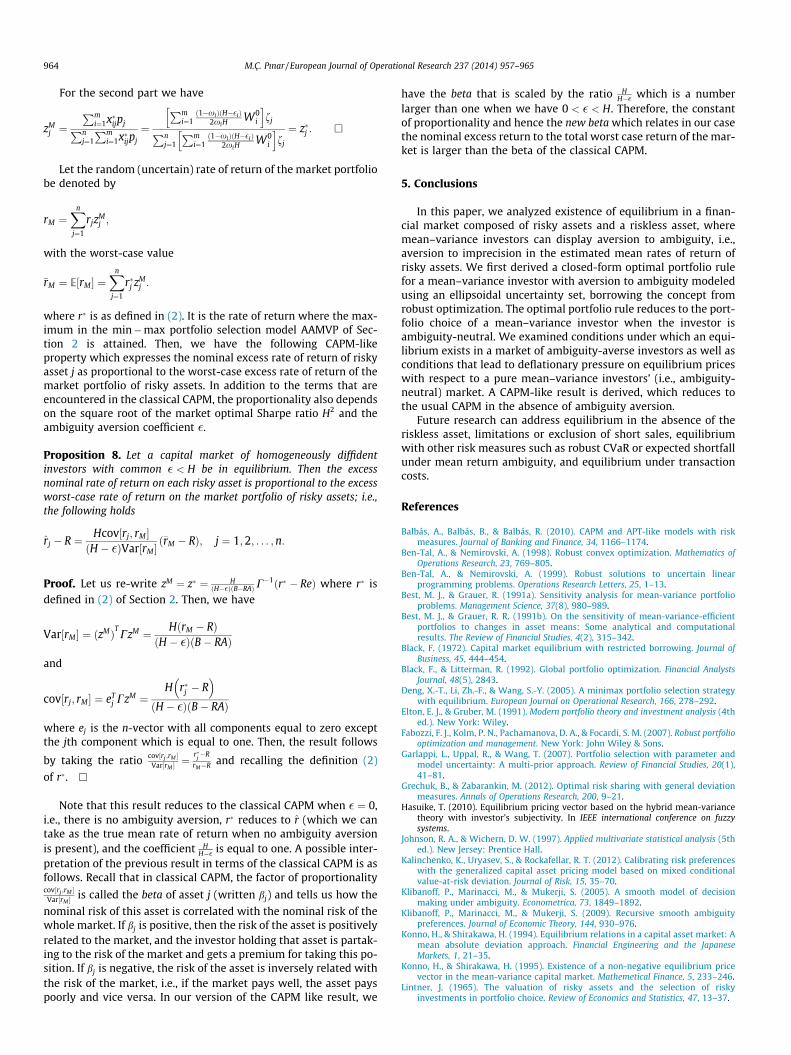
A Numerical Example. For illustration we consider an examplewith three investors and three assets (two risky assets and oneriskless asset). The relevant data for the risky assets are specifiedas follows

l̂ ¼ ð0:1287 0:1096ÞT

C ¼0:4218 0:05300:0530 0:2230

:

We assume x0j ¼ 10 for all three assets j ¼ 1;2;3, and the initial

portfolio holdings

½4 3 3�T ; ½6 2 2�T ; ½3 3 4�T

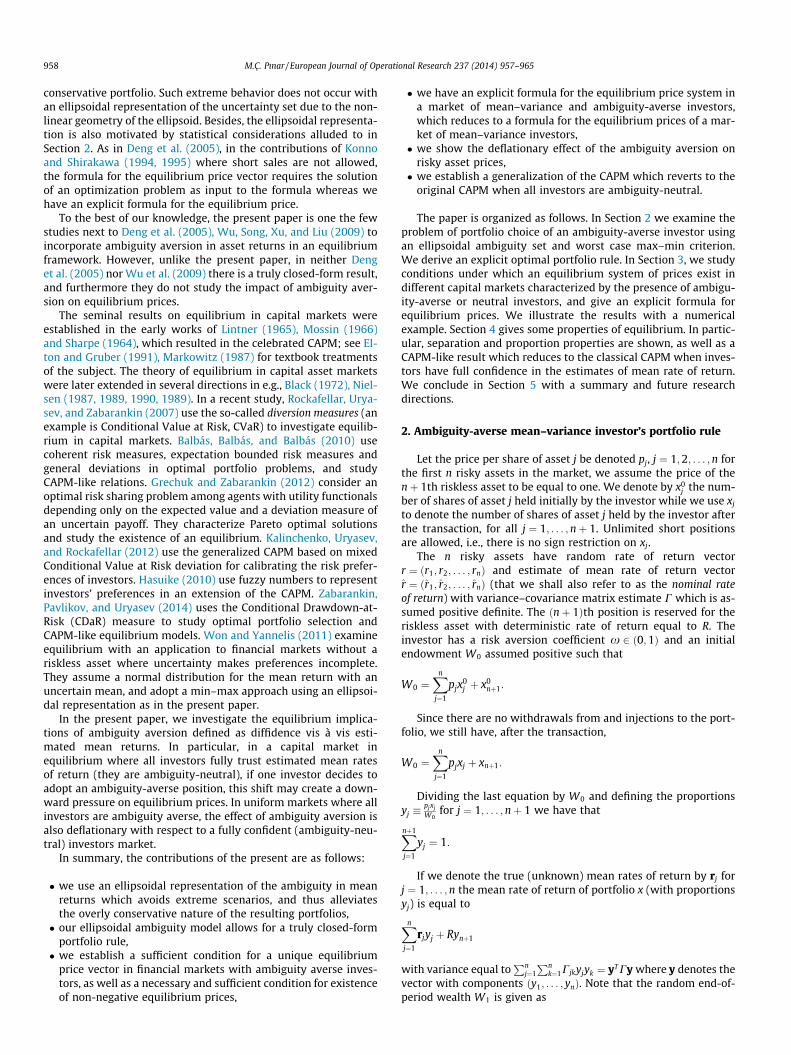
for each asset respectively, e.g., investor 1 holds initially 4 shares ofasset 1, 6 shares of asset 2 and 3 units of the riskless asset. We haveH ¼ 0:2822 and f ¼ C�1l̂ ¼ ½0:2509 0:4319�T . In Fig. 1 we plot the

0.2 0.3 0.4 0.5 0.6 0.7 0.8 0.9 10

5

10

15

20

25

30

35

40

45

50uniformly ambiguity−averse investors turn more risk−averse at epsilon=0.01

omega

pric

e

Fig. 1. Effect of increasing risk aversion coefficient x when all investors are equallyambiguity averse with �i ¼ 0:01 for i ¼ 1;2;3.

0 0.05 0.1 0.15 0.2 0.25 0.3 0.350

0.05

0.1

0.15

0.2

0.25

0.3

0.35al investors turn increasingly more ambiguity−averse at omega=0.5

epsilon

pric

e

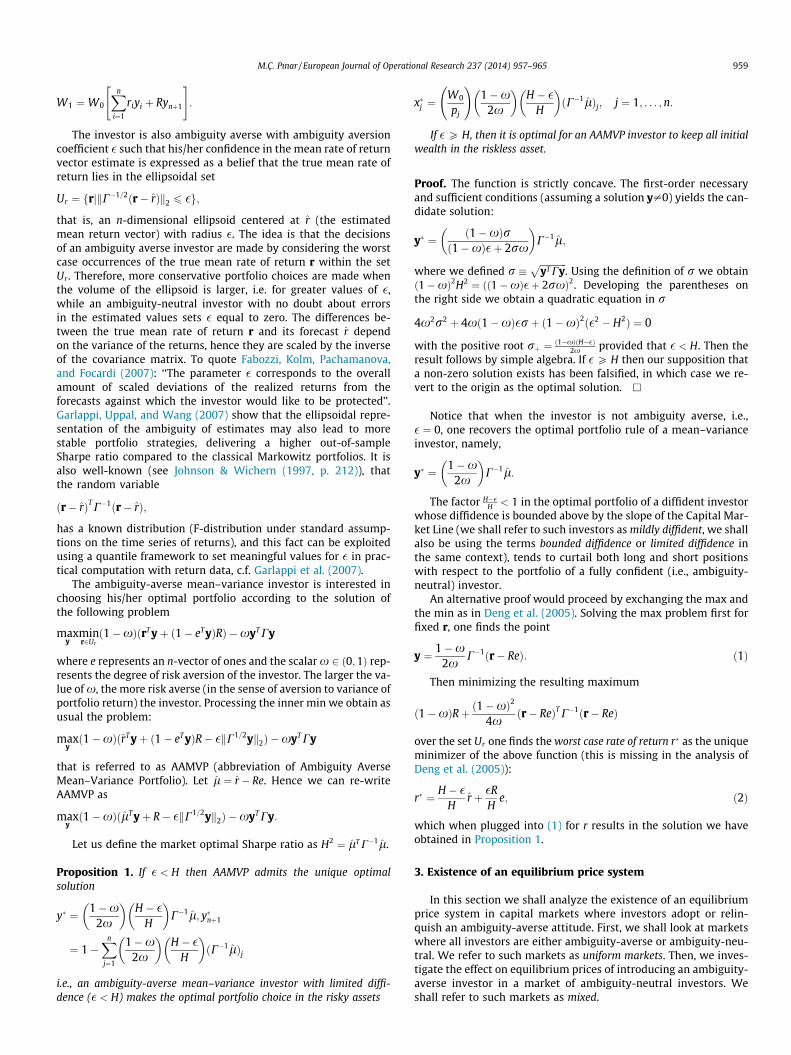
Fig. 3. Effect of increasing ambiguity aversion equally across the board withxi ¼ 0:5 for i ¼ 1;2;3.

962 M.Ç. Pınar / European Journal of Operational Research 237 (2014) 957–965

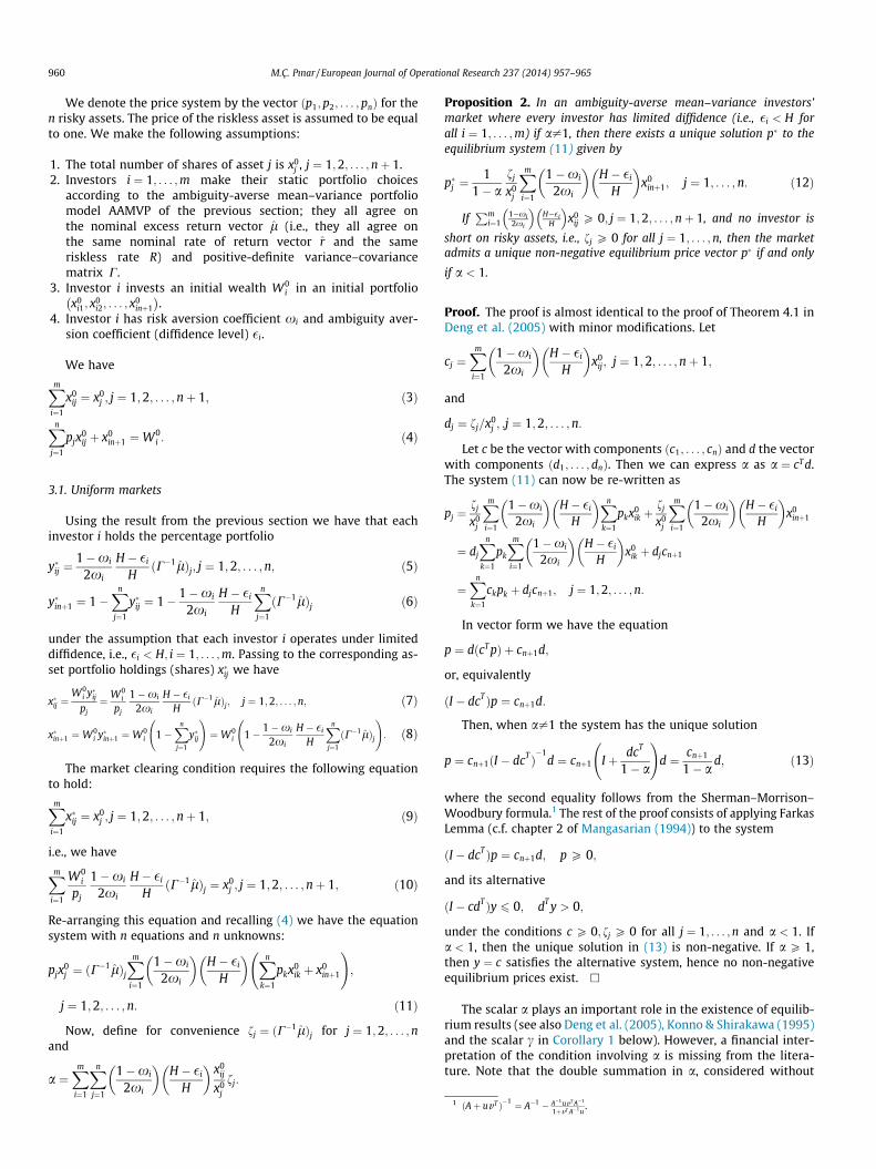
evolution of the prices of the two risky assets in a uniformly ambi-guity-averse investors’ market with �i ¼ 0:01 for i ¼ 1;2;3. Increas-ing x, i.e., increasing the risk aversion of investors (expressed as anincreasing emphasis on a smaller variance of portfolio return)equally for all investors while ambiguity aversion remains fixedacross the board has a sharp deflationary effect on asset prices. InFigs. 2 and 3 we show the impact of increasing ambiguity aversionequally for all investors at two different levels of risk aversion,x ¼ 0:25 and x ¼ 0:5, respectively. Both figures show clearly thedeflationary effect on asset prices of increasing ambiguity aversionat both levels of risk aversion. The decrease in prices in response toan increase in ambiguity aversion is much more pronounced whenthe investors are less risk-averse at x ¼ 0:25.

3.2. Mixed markets

Consider now a uniform market with ambiguity-neutral inves-tors where an investor decides to adopt an ambiguity-averse posi-tion. For simplicity we shall examine the case where we have twoinvestors. Investor indexed 1 is ambiguity-neutral with risk aver-sion coefficient x1, investor indexed 2 is ambiguity-averse with

0 0.05 0.1 0.15 0.2 0.25 0.3 0.350

5

10

15

20

25

30

35

40

45

50all investors turn increasingly more ambiguity=averse at omega=0.25

epsilon

pric

e

Fig. 2. Effect of increasing ambiguity aversion equally across the board withxi ¼ 0:25 for i ¼ 1;2;3.

coefficient � < H and risk aversion coefficient x2. All otherassumptions about the assets traded in the market are still valid.

The ambiguity-neutral investor makes the portfolio choice

x1j ¼W0

1

pj

1�x1

2x1fj; j ¼ 1; . . . ;n; x1nþ1 ¼W0

1 1� 1�x1

2x1

Xn

j¼1

fj

!;

while the ambiguity-averse investor makes the choice

x2j ¼W0

2

pj

ð1�x2ÞðH � �Þ2Hx2

fj; j ¼ 1; . . . ;n;

x2nþ1 ¼W02 1� ð1�x2ÞðH � �Þ

2Hx2

Xn

j¼1

fj

!:

As in the proof of Proposition 2 we define

c1j ¼

1�x1

2x1x0

1j j ¼ 1; . . . ;nþ 1;

for investor 1, and

~c2j ¼

1�x2

2x2

H � �H

x02j j ¼ 1; . . . ;nþ 1;

for investor 2, and dj ¼ fj=x0j for j ¼ 1; . . . ;n. Then we can express the

equilibrium price system for the mixed market as

pm ¼c1

nþ1 þ ~c2nþ1

1� am d;

where am ¼ dTðc1 þ ~c2Þ, and we assume that the conditions guaran-teeing the non-negativity of pm as expressed in Proposition 2 hold.

Now, we compare the equilibrium price system pm to the equi-librium price system of a uniform ambiguity-neutral investorsmarket. I.e., if investor 2 were to be ambiguity-neutral as well,we would have the following price system pp:

pp ¼c1

nþ1 þ c2nþ1

1� ap d;

where ap ¼ dTðc1 þ c2Þ with

c2j ¼

1�x2

2x2x0

2j j ¼ 1; . . . ;nþ 1:

We assume again the conditions guaranteeing the non-negativ-ity of pp expressed in Corollary 1 hold. Now, it is a simple exerciseto see that

M.Ç. Pınar / European Journal of Operational Research 237 (2014) 957–965 963

~c2j ¼

H � �H

c2j ; j ¼ 1; . . . ;nþ 1

and

am ¼ ap þ H � �H� 1

� �dT c2:

These observations imply that

pm ¼c1

nþ1 þ H��H c2

nþ1

1� ap þ 1� H��H

� �dT c2

d:

Therefore, if c2nþ1 > 0 and dT c2 > 0, we have pm < pp, i.e., if an

investor with positive initial holdings moves from ambiguity-neu-tral position to (bounded) ambiguity-averse position, this changehas a deflationary effect on equilibrium prices. We summarize thisresult below. We define

cij ¼

1�xi

2xix0

ij j ¼ 1; . . . ;nþ 1; i ¼ 1; . . . ;m

for every investor i, and refer to the n-vector with componentsci

1; . . . ; cin

� �as ci.

Proposition 5. In a uniform market of m ambiguity-neutral mean–variance investors in equilibrium, assume investor m adopts anambiguity-averse attitude with coefficient � < H. Then the followingstatements hold:

1. A non-negative equilibrium price system

pm ¼Pm�1

i¼1 cinþ1 þ ~cm

nþ1

1� amd

exists, if and only if am < 1 where am is defined as

am ¼ dTXm�1

i¼1

ci þ ~cm

!:

2. If the initial holdings x0mj for all j ¼ 1; . . . ;nþ 1 of investor m are

positive, the equilibrium prices of the mixed market are smallerthan the equilibrium prices of the uniform market.

The above result is not surprising if one bears in mind that anambiguity-averse investor holds smaller long positions in risky as-sets compared to an ambiguity-neutral investor, which leads to adecreased demand for risky assets, and hence exerts a downwardpressure on equilibrium prices.

A similar analysis can be made when the ambiguity aversion ofone investor is not classified as mildly diffident, but rather, signif-icantly diffident, i.e., with �P H, in which case this investor wouldput all his/her initial wealth into the riskless asset. It can be shownagain that such behavior leads to a drop in equilibrium prices. Thisis left as an exercise.

4. Properties of the equilibrium price system

We devote this section to the study of some interesting proper-ties of portfolios in equilibrium. More precisely, we follow the ref-erences Deng et al. (2005), Konno and Shirakawa (1994), Konnoand Shirakawa (1995) to examine the properties of the portfoliosin equilibrium in a market of mildly diffident mean–varianceinvestors. Define the master fund z�j ¼ fj=eTf for all j ¼ 1; . . . ;n.We begin with the following two-fund separation property. Let usdefine A ¼ eTC�1e and B ¼ eTC�1r̂.

Proposition 6. Let the price system in the mildly diffident mean–variance investors’ market be as defined in (12). Then, after thetransaction, each investor i holds

(i) a portfolio composed of the riskless asset and a non-negativemultiple ki of the initial total holdings x0 ¼ x0

1; x02; . . . ; x0

n

� �of

risky assets, wherePm

i¼1ki ¼ 1 and

ki ¼ð1� aÞW0

i ð1�xiÞðH � �iÞxiPm

k¼11�xkxkðH � �kÞx0

knþ1

for i ¼ 1; . . . ;m;(ii) a percentage portfolio which is a linear (ni;1� ni) combination

of the percentage riskless portfolio ð0;0; . . . ;0;1Þ and the (aug-mented) master fund z�1; z

�2; . . . ; z�n;0

� �consisting only of risky

assets where ni ¼ 1�xixi

H��H ðB� RAÞ.

Proof. Recall that in equilibrium each investor i holds the optimalportfolio

x�ij ¼W0

i ð1�xiÞðH � �iÞfj

2xiHp�j¼ W0

i ð1�xiÞðH � �iÞfj

2xi1

1�afj

x0j

Pmk¼1

1�xk2xkðH��kÞ

x0knþ1

¼W0i ð1�xiÞðH � �iÞð1� aÞ

xiPm

k¼11�xkxkðH � �kÞx0

knþ1

x0j :

Since we havePm

i¼1x�ij ¼ xj0, we infer immediately thatPm

i¼1ki ¼ 1. This proves part (i).For part (ii), recall that y�ij ¼

ð1�xiÞðH��iÞ2xiH

fj and

y�inþ1 ¼ 1� ð1�xiÞðH��iÞ2xiH

eTf. Since eTf ¼ B� RA, we can re-write

y�ij ¼ð1�xiÞðH��iÞ

2xiHðB� RAÞz�j and y�inþ1 ¼ 1� ð1�xiÞðH��iÞ

2xiHðB� RAÞ.

Hence, the result follows. h

We note that the weight ni in part (ii) of the previous result is smallerthanthecorrespondingweightthatwouldresult if�i weretakenequaltozero, i.e., the investor were ambiguity-neutral. This observation impliesthat ambiguity aversion leads to giving less weight to master fund z�.

Let the vector yM and zM be defined with components

yMj ¼

x0j pjPnþ1

j¼1 x0j pj

; j ¼ 1;2; . . . ;nþ 1;

and

zMj ¼

x0j pjPnþ1

j¼1 x0j pj

; j ¼ 1;2; . . . ;n;

called, respectively, the market portfolio of all assets and the mar-ket portfolio of risky assets in Deng et al. (2005). We also havethe following proportion property.

Proposition 7. Let the capital market be in equilibrium. Then thefollowing hold:

(i) the market portfolio yM is proportional to the market portfoliozM of risky assets;

(ii) the market portfolio zM of risky assets is identical to z�.

Proof. Using the definition of yM we have

yMj ¼

Pmi¼1x�ijpjPn

j¼1

Pmi¼1x�ijpj þ

Pmi¼1x�inþ1

¼Pm

i¼1ð1�xiÞðH��iÞ

2xiHW0

i

h ifjPn

j¼1

Pmi¼1ð1�xiÞðH��iÞ

2xiHW0

i

h ifj þ

Pmi¼1W0

i 1� ð1�xiÞðH��iÞ2xiH

etf� �

¼Pm

i¼1ð1�xiÞðH��iÞ

2xiHW0

i

h ifjPm

i¼1W0i

¼ðB� RAÞ

Pmi¼1ð1�xiÞðH��iÞ

2xiHW0

i

h iPm

i¼1W0i

z�j :

964 M.Ç. Pınar / European Journal of Operational Research 237 (2014) 957–965

For the second part we have

zMj ¼

Pmi¼1x�ijpjPn

j¼1

Pmi¼1x�ijpj

¼Pm

i¼1ð1�xiÞðH��iÞ

2xiHW0

i

h ifjPn

j¼1

Pmi¼1ð1�xiÞðH��iÞ

2xiHW0

i

h ifj

¼ z�j : �

Let the random (uncertain) rate of return of the market portfoliobe denoted by

rM ¼Xn

j¼1

rjzMj ;

with the worst-case value

�rM ¼ E½rM� ¼Xn

j¼1

r�j zMj :

where r� is as defined in (2). It is the rate of return where the max-imum in the min�max portfolio selection model AAMVP of Sec-tion 2 is attained. Then, we have the following CAPM-likeproperty which expresses the nominal excess rate of return of riskyasset j as proportional to the worst-case excess rate of return of themarket portfolio of risky assets. In addition to the terms that areencountered in the classical CAPM, the proportionality also dependson the square root of the market optimal Sharpe ratio H2 and theambiguity aversion coefficient �.

Proposition 8. Let a capital market of homogeneously diffidentinvestors with common � < H be in equilibrium. Then the excessnominal rate of return on each risky asset is proportional to the excessworst-case rate of return on the market portfolio of risky assets; i.e.,the following holds

r̂j � R ¼ Hcov½rj; rM �ðH � �ÞVar½rM�

ð�rM � RÞ; j ¼ 1;2; . . . ;n:

Proof. Let us re-write zM ¼ z� ¼ HðH��ÞðB�RAÞC

�1ðr� � ReÞ where r� isdefined in (2) of Section 2. Then, we have

Var½rM� ¼ ðzMÞTCzM ¼ HðrM � RÞðH � �ÞðB� RAÞ

and

cov½rj; rM� ¼ eTj CzM ¼

H r�j � R� �

ðH � �ÞðB� RAÞ

where ej is the n-vector with all components equal to zero exceptthe jth component which is equal to one. Then, the result follows

by taking the ratio cov½rj ;rM �Var½rM �

¼r�

j�R

�rM�R and recalling the definition (2)

of r�. h

Note that this result reduces to the classical CAPM when � ¼ 0,i.e., there is no ambiguity aversion, r� reduces to r̂ (which we cantake as the true mean rate of return when no ambiguity aversionis present), and the coefficient H

H�� is equal to one. A possible inter-pretation of the previous result in terms of the classical CAPM is asfollows. Recall that in classical CAPM, the factor of proportionalitycov½rj ;rM �

Var½rM �is called the beta of asset j (written bj) and tells us how the

nominal risk of this asset is correlated with the nominal risk of thewhole market. If bj is positive, then the risk of the asset is positivelyrelated to the market, and the investor holding that asset is partak-ing to the risk of the market and gets a premium for taking this po-sition. If bj is negative, the risk of the asset is inversely related withthe risk of the market, i.e., if the market pays well, the asset payspoorly and vice versa. In our version of the CAPM like result, we

have the beta that is scaled by the ratio HH�� which is a number

larger than one when we have 0 < � < H. Therefore, the constantof proportionality and hence the new beta which relates in our casethe nominal excess return to the total worst case return of the mar-ket is larger than the beta of the classical CAPM.

5. Conclusions

In this paper, we analyzed existence of equilibrium in a finan-cial market composed of risky assets and a riskless asset, wheremean–variance investors can display aversion to ambiguity, i.e.,aversion to imprecision in the estimated mean rates of return ofrisky assets. We first derived a closed-form optimal portfolio rulefor a mean–variance investor with aversion to ambiguity modeledusing an ellipsoidal uncertainty set, borrowing the concept fromrobust optimization. The optimal portfolio rule reduces to the port-folio choice of a mean–variance investor when the investor isambiguity-neutral. We examined conditions under which an equi-librium exists in a market of ambiguity-averse investors as well asconditions that lead to deflationary pressure on equilibrium priceswith respect to a pure mean–variance investors’ (i.e., ambiguity-neutral) market. A CAPM-like result is derived, which reduces tothe usual CAPM in the absence of ambiguity aversion.

Future research can address equilibrium in the absence of theriskless asset, limitations or exclusion of short sales, equilibriumwith other risk measures such as robust CVaR or expected shortfallunder mean return ambiguity, and equilibrium under transactioncosts.

References

Balbás, A., Balbás, B., & Balbás, R. (2010). CAPM and APT-like models with riskmeasures. Journal of Banking and Finance, 34, 1166–1174.

Ben-Tal, A., & Nemirovski, A. (1998). Robust convex optimization. Mathematics ofOperations Research, 23, 769–805.

Ben-Tal, A., & Nemirovski, A. (1999). Robust solutions to uncertain linearprogramming problems. Operations Research Letters, 25, 1–13.

Best, M. J., & Grauer, R. (1991a). Sensitivity analysis for mean-variance portfolioproblems. Management Science, 37(8), 980–989.

Best, M. J., & Grauer, R. R. (1991b). On the sensitivity of mean-variance-efficientportfolios to changes in asset means: Some analytical and computationalresults. The Review of Financial Studies, 4(2), 315–342.

Black, F. (1972). Capital market equilibrium with restricted borrowing. Journal ofBusiness, 45, 444–454.

Black, F., & Litterman, R. (1992). Global portfolio optimization. Financial AnalystsJournal, 48(5), 2843.

Deng, X.-T., Li, Zh.-F., & Wang, S.-Y. (2005). A minimax portfolio selection strategywith equilibrium. European Journal on Operational Research, 166, 278–292.

Elton, E. J., & Gruber, M. (1991). Modern portfolio theory and investment analysis (4thed.). New York: Wiley.

Fabozzi, F. J., Kolm, P. N., Pachamanova, D. A., & Focardi, S. M. (2007). Robust portfoliooptimization and management. New York: John Wiley & Sons.

Garlappi, L., Uppal, R., & Wang, T. (2007). Portfolio selection with parameter andmodel uncertainty: A multi-prior approach. Review of Financial Studies, 20(1),41–81.

Grechuk, B., & Zabarankin, M. (2012). Optimal risk sharing with general deviationmeasures. Annals of Operations Research, 200, 9–21.

Hasuike, T. (2010). Equilibrium pricing vector based on the hybrid mean-variancetheory with investor’s subjectivity. In IEEE international conference on fuzzysystems.

Johnson, R. A., & Wichern, D. W. (1997). Applied multivariate statistical analysis (5thed.). New Jersey: Prentice Hall.

Kalinchenko, K., Uryasev, S., & Rockafellar, R. T. (2012). Calibrating risk preferenceswith the generalized capital asset pricing model based on mixed conditionalvalue-at-risk deviation. Journal of Risk, 15, 35–70.

Klibanoff, P., Marinacci, M., & Mukerji, S. (2005). A smooth model of decisionmaking under ambiguity. Econometrica, 73, 1849–1892.

Klibanoff, P., Marinacci, M., & Mukerji, S. (2009). Recursive smooth ambiguitypreferences. Journal of Economic Theory, 144, 930–976.

Konno, H., & Shirakawa, H. (1994). Equilibrium relations in a capital asset market: Amean absolute deviation approach. Financial Engineering and the JapaneseMarkets, 1, 21–35.

Konno, H., & Shirakawa, H. (1995). Existence of a non-negative equilibrium pricevector in the mean-variance capital market. Mathemetical Finance, 5, 233–246.

Lintner, J. (1965). The valuation of risky assets and the selection of riskyinvestments in portfolio choice. Review of Economics and Statistics, 47, 13–37.

M.Ç. Pınar / European Journal of Operational Research 237 (2014) 957–965 965

Mangasarian, O. L. (1994). Nonlinear programming. In Classics in appliedmathematics. Philadelphia: SIAM.

Markowitz, H. M. (1987). Mean-variance analysis in portfolio choice and capitalmarkets. Cambridge: Basil Blackwell.

Mossin, J. (1966). Equilibrium in capital asset markets. Econometrica, 34, 768–783.Nielsen, L. T. (1987). Portfolio selection in the mean-variance model: A note. Journal

of Finance, 42, 1371–1376.Nielsen, L. T. (1989). Asset market equilibrium with short selling. Review of

Economic Studies, 56, 467–474.Nielsen, L. T. (1989). Existence of equilibrium in a CAPM. Journal of Economic Theory,

57, 315–324.Nielsen, L. T. (1990). Equilibrium in a CAPM without a riskless asset. Review of

Economic Studies, 57, 315–324.Panik, M. J. (1993). Fundamentals of convex analysis: Duality, separation,

representation and resolution. Berlin: Springer-Verlag.

Rockafellar, R. T., Uryasev, S., & Zabarankin, M. (2007). Equilibrium with investorsusing a diversity of deviation measures. Journal of Banking and Finance, 31,3251–3268.

Sharpe, W. F. (1964). Capital asset prices: A theory of market equilibrium undercondition of risk. Journal of Finance, 19, 425–442.

Stiemke, E. (1915). Über positive Lösungen homogener linearer Gleichungen.Mathematische Annalen, 76, 340–342.

Won, D. C., & Yannelis, N. C. (2011). Equilibrium theory with satiable and non-ordered preferences. Journal of Mathematical Economics, 47(Issue 2), 245–250.

Wu, Z.-W., Song, X.-F., Xu, Y.-Y., & Liu, K. (2009). A note on a minimax rule forportfolio selection and equilibrium price system. Applied Mathematics andComputation, 208, 49–57.

Zabarankin, M., Pavlikov, K., & Uryasev, S. (2014). Capital Asset Pricing Model(CAPM) with drawdown measure. European Journal of Operational Research,234(2), 508–517.