equations of motion ii: basics - pennsylvania … · john h. challis - modeling in biomechanics...
TRANSCRIPT

John H. Challis - Modeling in Biomechanics
4A-1
EQUATIONS OF MOTION II: BASICS
Overview• Equations of Motion• Mechanical Approaches
Newton-EulerLagrangianOthers
• Example I – A Single Rigid Body• Mechanical Basics• Example II – Two Rigid Bodies• General Format of Equations of Motion• Matrix Inversion
Analytical SolutionsNumerical SolutionsSingular Systems
• Mechanical Approaches - Summary
“There is no more common error than to assume that,because prolonged and accurate mathematicalcalculations have been made the application of theresults to some fact of nature is absolutely certain.”Alfred North Whitehead (1861-1947)

John H. Challis - Modeling in Biomechanics
4A-2
EQUATIONS OF MOTION
Equations of Motion – set of mathematicalequations which describe the forces and movements ofa body.
Inverse Dynamics – starting from the motion of thebody determines the forces and moments causing themotion.Process: measure joint displacements, differentiate toobtain velocities and accelerations, use Newton’s Lawsto compute forces and moments acting on body.
Direct Dynamics – starting from the forces andmoments acting on a body determines the motionarising from these forces and moments. (Also calledforward dynamics.)Process: “obtain” moments and forces acting at joints,integrate to obtain joint displacements.

John H. Challis - Modeling in Biomechanics
4A-3
MECHANICAL APPROACHESAlthough conservation laws can be invoked mostcommon approach is to consider forces and momentsacting on a body, and use these to determine equationsof motion.
Two main approaches are
Newton-EulerNewton amF∑ = .Euler ∑ == θα ��.. IIT (2D case only)
LagrangianLagrangian Equation PKL −=
Equation of Motion TqL
qL
dtd =−
∂∂
∂∂�
(Non-conservative)
Others Methods• Kane’s Method• Gibbs-Appell• Jourdain

John H. Challis - Modeling in Biomechanics
4A-4
EXAMPLE I – A SINGLE RIGID BODYThe net effect of all forces acting on a rigid body isequal to the product of the mass of the segment and theacceleration of the center of mass.
a.mFi ====∑∑∑∑
a.mFFF 321 ====++++++++
Whereg.mF3 ====
m.g
F1
F2
m.a
John H. Challis - Modeling in Biomechanics
4A-5
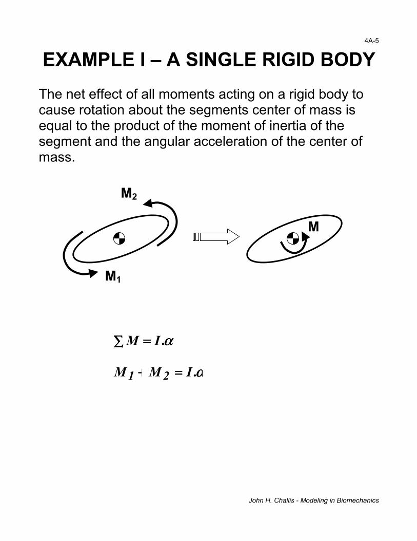
EXAMPLE I – A SINGLE RIGID BODYThe net effect of all moments acting on a rigid body tocause rotation about the segments center of mass isequal to the product of the moment of inertia of thesegment and the angular acceleration of the center ofmass.
αααα.IM ====∑∑∑∑
αααα.IMM 21 ====++++
M2
M1
M

4A-6
EXAMPLE I – A SINGLE RIGID BODY
M∑
θθθθ ====��
WhereJM - a
m - mag - accL - dist
of mθθθθ - angI - momθθθθ�� - ang
θθθθ
L
y
MJ
John H. Challis - Modeling in Biomechanics
( ) θαθ ��..cos... IILgmMJ ==+=
(((( ))))[[[[ ]]]] I/cos.L.g.mMJ θθθθ++++
pplied moment at jointss of the segmenteleration due to gravityance from joint center to segment center
assle of segment to horizontalent of inertia of segment
ular acceleration
mgx

John H. Challis - Modeling in Biomechanics
4A-7
MECHANICAL BASICS
Mechanical Degrees of Freedom - refers to thenumber of independent coordinates required to specifythe location of a body or system of bodies.
Mechanical degrees of freedom for thearm?
Shoulder three degrees of freedomElbow two degrees of freedomWrist two degrees of freedom
Total Degrees of Freedom - 7
So in theory for the whole upper limb sevengeneralized coordinates should specify thelocation of the arm. Standard mechanical analysesstart with specifying the x, y, z coordinates of eachsegments center of mass, and the three angles (6 x 3 =18).

John H. Challis - Modeling in Biomechanics
4A-8
MECHANICAL BASICSGeneralized Coordinates - refers to the minimumnumber of number of independent coordinates neededto specify the motion of a body. There are often manysets of generalized coordinates for a given system, buta prudent choice can simplify the analysis significantly.
q - generalized coordinateq� - generalized velocityq�� - generalized acceleration
Example
(((( ))))θθθθcos.Lx ====
(((( ))))θθθθsin.Ly ====
(((( ))))θθθθθθθθ cos.. �� Lx −−−−====
(((( ))))θθθθθθθθ sin.. �� Ly ====
So we can reduce the number of variables required inthe equations of motion by such substitutions.
θθθθ
x x
y
y

John H. Challis - Modeling in Biomechanics
4A-9
MECHANICAL BASICS
Kinetic Energy – the energy possessed by a bodydue to its motion.
221 vmKL .==== linear kinetic energy
221 ωωωω.IKA ==== rotational kinetic energy
Potential Energy – the energy posed by a body dueto its position.
hgmP ..====
[For a conservative system ====++++++++ PKK AL constant, soif potential energy increases then kinetic energy mustdecrease, and vice versa.]

John H. Challis - Modeling in Biomechanics
4A-10
MECHANICAL BASICS
Centripetal Force – a force causing a body todeviate from its motion in a straight line to motion alonga curved path. For motion about a radius (r ) thecentripetal force acts towards the center of the circle
rmrmrvmFCent ..... 22
2θω �===
[Centrifugal force – an inertial force acting in oppositedirection to centripetal force.]
Coriolis Force – (after G.G de Coriolis, 1792-1843)is a force acting on a body perpendicular to the axis ofrotation and the direction of motion of the body.
θω �...2...2 vmvmFCor ==

4A-11
EXAMPLE II - TWO RIGID BODIES
Whereiθθθθ - angliL - lengim - mascmiL - dis
iI - mom
Lcm1
2222
θθθθ
Jo
e of ith segmentth of ith segments of ith segmenttance from joint cenmass for ith segmenent of inertia of ith s
1111
θθθθ
Lcmhn H. Challis - Modeling in Biomechanics
ter to center oftegment

John H. Challis - Modeling in Biomechanics
4A-12
EXAMPLE II - TWO RIGID BODIES
( ) ( ) ( )θθθθθ G,v.MT ++= ���
(((( )))) (((( ))))[[[[ ]]]] 22212
22121
21111 2 ILLLLmILmM cmcmcm ++++++++++++++++++++==== θθθθθθθθ cos....,
(((( )))) (((( )))) 22
22221221 ILmLLmM cmcm ++++++++==== .cos..., θθθθθθθθ
(((( )))) (((( )))) 22
22221212 ILmLLmM cmcm ++++++++==== .cos..., θθθθθθθθ
(((( )))) 22222,2 . ILmM cm ++++====θθθθ
(((( )))) (((( )))) (((( ))))2221221211 2 θθθθθθθθθθθθθθθθθθθθ ���� ++++−−−−==== ...sin..., cmLLmv
(((( )))) (((( )))) 21221221 θθθθθθθθθθθθ �� .sin..., cmLLmv ====
(((( )))) (((( )))) (((( )))) (((( ))))[[[[ ]]]]11212211111 θθθθθθθθθθθθθθθθθθθθ cos.cos...cos..., LLgmgLmG cmcm ++++++++++++====(((( )))) (((( ))))212221 θθθθθθθθθθθθ ++++==== cos..., cmLgmG

John H. Challis - Modeling in Biomechanics
4A-13
EXAMPLE II - TWO RIGID BODIES• For each link there is a second order non-linear
differential equation describing the relationshipbetween the moments and angular motion of the twolink system.
• Terms from adjacent links occur in the equations for alink – the equations are coupled. For example(((( )))) (((( )))) (((( )))) (((( ))))[[[[ ]]]]11212211111 θθθθθθθθθθθθθθθθθθθθ cos.cos...cos..., LLgmgLmG cmcm ++++++++++++====
• Group all the terms including moment of inertia –gives the inertia matrix.
• The inertia matrix is symmetric and positive definite.Matrices having these properties are normallyinvertible.
• Group all terms involving angular velocity, gives termsdealing with centripetal and Coriolis forces
• Group all terms relating to gravity – gives vector ofgravity terms.

John H. Challis - Modeling in Biomechanics
4A-14
GENERAL FORMAT OF EQUATIONSOF MOTION
Equation for Inverse Dynamics
( ) ( ) ( )θθθθθ G,v.MT ++= ���
WhereT - vector of joint moments (n x 1)
( )θM - inertia matrix (n x n)( )θθ �,v - vector of centrifugal/Coriolis terms (n x 1)( )θG - vector of gravity terms
and n is the number of joints in the system
Re-arrange equation for Direct Dynamics
(((( )))) (((( )))) (((( ))))(((( ))))θθθθθθθθθθθθθθθθθθθθ G,vT.M 1 −−−−−−−−==== −−−− ���
n = 1 no matrix inversion required, simple to perform
n > 1 then you require an inversion of the mass matrix

John H. Challis - Modeling in Biomechanics
4A-15
MATRIX INVERSIONA matrix is just a rectangular array of numbers orsymbols organized into rows and columns, for example
( ) ( )( ) ( )
−
=θθθθ
cossinsincos
]A[
=
666.0125.033.025.0
]A[
Given the equation,a.mF =
if we know the force and the acceleration we can workout the mass from
aFm =
For matrices division does not exist so we use theinverse
F.am 1−=
Properties of an Inverse MatrixIf ]A[ is a matrix with an equal number of rows andcolumns then
]I[]A].[A[]A.[]A[ 11 == −−
Where ]I[ is the identity matrix (matrix equivalent of 1)

John H. Challis - Modeling in Biomechanics
4A-16
MATRIX INVERSIONANALYTICAL SOLUTIONS
For certain matrices the inverse can be computedanalytically, for example
( ) ( )( ) ( )
−
=θθθθ
cossinsincos
]A[
( ) ( )( ) ( )
−
=−θθθθ
cossinsincos
]A[ 1
=−
1001
]A.[]A[ 1
Such calculations can be done by hand (tricky) or via asymbolic algebraic manipulation package (e.g. MAPLE).

John H. Challis - Modeling in Biomechanics
4A-17
MATRIX INVERSIONNUMERICAL SOLUTIONS
If an analytical solution does not exist then there arevarious numerical techniques. For example
=
666.0125.033.025.0
]A[
−
−=−
9960.19980.06347.23174.5
]A[ 1
[ ]I1001
]A.[]A[ 1 =
=−
Question: What are the numerical techniques fornumerically inverting a matrix?

John H. Challis - Modeling in Biomechanics
4A-18
MATRIX INVERSIONNUMERICAL SOLUTIONS
There are a variety of techniques for the numericalinversion of a matrix, including
• Gaussian Elimination (Gauss-Seidel, LU factorization)
• Cholesky Factorization (symmetric definite matrices)
• Singular Value Decomposition
Numerically more robust routines are more timeconsuming, numerically less robust may consider amatrix singular when this is not the case.

John H. Challis - Modeling in Biomechanics
4A-19
MATRIX INVERSIONNUMERICAL SOLUTIONS
Algorithms to invert a matrix are readily available thetrade-off must be made between numerical robustnessand time for computation.
In MATLAB for example to solve,[ ]B]x].[A[ =
where ]x[ is unknown, you can write
>x=A\B
This perform the following matrix operation[ ]B.]A[]x[ 1−=
Sparse Matrices – these arise in certainapplications where a large number of the matrixelements are zero. Special algorithms are available tosolve these problems.
John H. Challis - Modeling in Biomechanics
4A-20
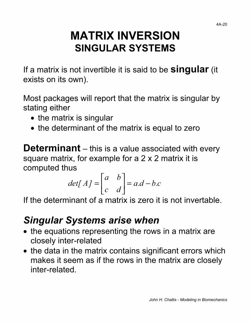
MATRIX INVERSIONSINGULAR SYSTEMS
If a matrix is not invertible it is said to be singular (itexists on its own).
Most packages will report that the matrix is singular bystating either
• the matrix is singular• the determinant of the matrix is equal to zero
Determinant – this is a value associated with everysquare matrix, for example for a 2 x 2 matrix it iscomputed thus
c.bd.adcba
]Adet[ −=
=
If the determinant of a matrix is zero it is not invertable.
Singular Systems arise when• the equations representing the rows in a matrix are
closely inter-related• the data in the matrix contains significant errors which
makes it seem as if the rows in the matrix are closelyinter-related.

John H. Challis - Modeling in Biomechanics
4A-21
MECHANICAL APPROACHES -SUMMARY
• Silver (1982) has shown that equations of the sameform can be derived using Lagrange or Newton-Eulermethods if constraints are imposed when using theNewton-Euler approach.
• Theoretically the same equivalence can be shownbetween equations derived from other formulations(e.g. Kane's method).
• Given the equivalence of formulations what becomesimportant is how easily the equations of motion canbe formed if the researcher wants to examine avariety of different mechanical systems, and ease ofcomputer implementation.
• Ease of formulation often depends on selection ofappropriate generalized coordinates.

John H. Challis - Modeling in Biomechanics
4A-22
REVIEW QUESTIONS1. Write the equations which describe the Newton-Euler
approach to formulation of the equations of motion ofa mechanical system?
2. Write the equations which describe the Lagrangianapproach to formulation of the equations of motion ofa mechanical system?
3. What is meant by the term mechanical degrees offreedom?
4. What is meant by the term generalized coordinates?
5. Describe the relationship between kinetic andpotential energy for a conservative system.
6. Write the equation for direct dynamics in matrix andvector form.
7. List techniques which could be used to invert anumerical matrix.
8. What does it mean if a matrix is singular?