eps allowable stress calculations (rev. 2) - civil...

Steven F. Bartlett, 2013

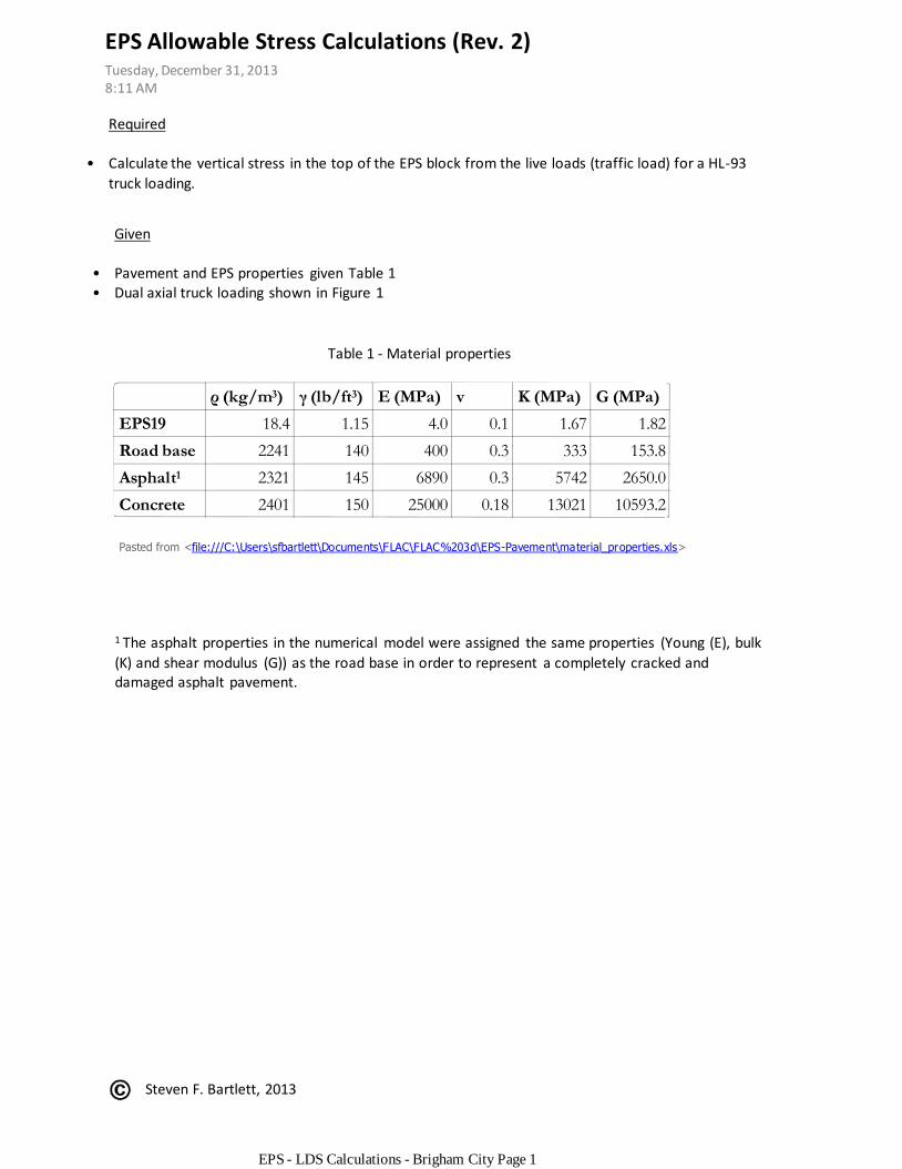
Required

Calculate the vertical stress in the top of the EPS block from the live loads (traffic load) for a HL-93

truck loading.

•

Given

Pavement and EPS properties given Table 1•Dual axial truck loading shown in Figure 1•

Table 1 - Material properties

1 The asphalt properties in the numerical model were assigned the same properties (Young (E), bulk

(K) and shear modulus (G)) as the road base in order to represent a completely cracked and damaged asphalt pavement.

ρ (kg/m3) γ (lb/ft3) E (MPa) v K (MPa) G (MPa)

EPS19 18.4 1.15 4.0 0.1 1.67 1.82

Road base 2241 140 400 0.3 333 153.8

Asphalt1 2321 145 6890 0.3 5742 2650.0

Concrete 2401 150 25000 0.18 13021 10593.2

Pasted from <file:///C:\Users\sfbartlett\Documents\FLAC\FLAC%203d\EPS-Pavement\material_properties.xls>

EPS Allowable Stress Calculations (Rev. 2)Tuesday, December 31, 20138:11 AM

EPS - LDS Calculations - Brigham City


Fig. 1 - HL-93 Dual Axial Loading - 25 kip per axial with spacing of 4 ft between axels

Assumptions / Approach

Materials behave within the elastic range and the properties in Table 1 are appropriate for this range•Tire loading converted to equivalent square loading in an area 0.3 m x 0.3 m = 0.09 m2•3D model•Width of roadway is 13 m with 3 lanes (x-direction)•Length of roadway = continuous roadway = approximated by 39 m length (y-direction)•

Base = fixed (fixed z)○

Sides = free (free x, y, z)○

Ends = fixed (fixed y)○

Boundary conditions•

For a single 25-kip axial with dual tires, the contact area can be estimated by converting the set of

duals into a singular area by assuming that the singular area has an area equal to the contact area of the duals.

•

q = QD / ACD Eq. (1) ○

Dual Tire Loading(single axial/one side)

QD = 12.5 kips 55.6 KN

q = 90 psi 618 Kpa

ACD = 139 in^2 0.09 m2

Table 2 - HL-93 tire loading

End ViewDual Axel Side View

The 618 kPa vertical stress from the 12.5 kip loading will be put into the numerical modeling to

determine the stress redistribution in the pavement section and into the EPS. This stress will be applied over a circular area representing the dual tire at the top of the pavement is 0.17 m.

EPS Calculations (cont.)Tuesday, December 31, 201311:43 AM



Numerical model and boundary conditions

Nodal spacing

x-direction (width) = 13 m / 52 nodes = 0.25 m per node•y-direction (length) = 39 m / 130 nodes = 0.3 m per node•x-direction (height) = 3 m / 20 nodes = 0.15 m per node•

Material Property assignment (see Table 1)

top 3 layer = road base (red)•4th layer = load distribution slab (reinforced concrete) (green)•5th to 20th layer = EPS19•

all bottom nodes fixed (z)

z

x

y

end nodes fixed (y)

end nodes fixed (y)

free (x and y)free (x and y)




Model Properties




Load Application (12,5 kip tire loads)

12.5 k12.5 k

12.5 k 12.5 k

12.5 k vertical loadings applied to the model

truck 1




Load Application (sleeper slab)

length of approach slab = 25.5 feet = 7.77 m•width of approach slab = 42 feet 10 inches = 13.05 m•width of sleeper slab = 5 feet = 1.5 m•stress from sleeper slab at base of footing = 150 k / 5 feet / 42.83 ft = 700.4 psf = 33.6 kPa (from

150 k tire loads only)

•

FLAC3D 3.10

Itasca Consulting Group, Inc.Minneapolis, MN USA

©2006 Itasca Consulting Group, Inc.

Step 21515 Model Perspective07:51:39 Tue Dec 31 2013

Center: X: 6.500e+000 Y: 1.950e+001 Z: 0.000e+000

Rotation: X: 15.000 Y: 0.000 Z: 20.000

Dist: 9.089e+001 Mag.: 1.25Ang.: 22.500

Plane Origin: X: 6.500e+000 Y: 1.950e+001 Z: 2.990e+000

Plane Normal: X: 0.000e+000 Y: 0.000e+000 Z: 1.000e+000

Contour of SZZ Plane: on Magfac = 0.000e+000 Live mech zones shown Gradient Calculation

-3.3590e+004 to -3.0000e+004-3.0000e+004 to -2.5000e+004-2.5000e+004 to -2.0000e+004-2.0000e+004 to -1.5000e+004-1.5000e+004 to -1.0000e+004-1.0000e+004 to -5.0000e+003-5.0000e+003 to 0.0000e+000 0.0000e+000 to 7.6496e+002

Interval = 5.0e+003

33.6 kPa stress applied over 1.5 m strip sleeper slab




Results - 12 kip tire load - top of EPS

Plan view of plane cut horizontally through model at top of EPS layer (z = 2.4 m). The maximum stress

from the tire loading is -1.7e4 Pa (negative means acting downward). This converts to:

1.74e4 Pa / 1000 Pa / Kpa / 96 kPa / 1 tsf * 2000 psf / tsf / 144 psf / psi = 2.5 psi




Results - 12 kip tire load - X-section view

X-sectional view of plane cut vertical through model at rear axial load (i.e., y - 18.75 m). EPS layer is

the 5th layer (top to bottom). The maximum stress from the tire loading is between 10 and 20 kPa.

Top of EPS layer vertical stress between -1.0e4 and -2.0e4 Pa



© Steven F. Bartlett, 2013

Results - 150 k tire load on sleeper slab - results on top of EPS

Plan view of plane cut horizontally through model at top of EPS layer (z = 2.4 m). The maximum stress

from the tire loading is -1.5e4 Pa (negative means acting downward). This converts to:

1.5e4 Pa / 1000 Pa / Kpa / 96 kPa / 1 tsf * 2000 psf / tsf / 144 psf / psi = 2.17 psi ( from 150 k tire load

only)

FLAC3D 3.10



Step 21515 Model Perspective08:16:51 Tue Dec 31 2013

Center: X: 6.500e+000 Y: 1.950e+001 Z: 1.500e+000

Rotation: X: 15.000 Y: 0.000 Z: 20.000

Dist: 9.089e+001 Mag.: 1.95Ang.: 22.500




-2.4071e+004 to -2.2500e+004-2.2500e+004 to -2.0000e+004-2.0000e+004 to -1.7500e+004-1.7500e+004 to -1.5000e+004-1.5000e+004 to -1.2500e+004-1.2500e+004 to -1.0000e+004-1.0000e+004 to -7.5000e+003-7.5000e+003 to -5.0000e+003-5.0000e+003 to -2.5000e+003-2.5000e+003 to 0.0000e+000

EPS Calculations (cont.)Tuesday, December 31, 20132:32 PM



Results - 150 k load applied to sleeper slab - X-section view

X-sectional view of plane cut vertical through middle of sleeper slab footing (i.e., y = 7.75 m). EPS

layer is the 5th layer (top to bottom). The maximum stress from the tire loading is between 10 and 20 kPa.

Top of EPS layer vertical stress between

Top of EPS layer vertical stress between -1.0e4 and -1.5e4 Pa




Live load calculations - Controlling case

LL tire = 2.5 psi (from FLAC for minimal pavement thickness section) LL Lane load = 3 lanes x 10 ft per line / 39 * 0.65 klf /10 ft wide lane = 0.05 ksf or 50 psf or 0.35 psi

Dead load calculations

ρ γ E v K G thickness v. stress

(kg/m3) (lb/ft3) (MPa) (MPa) (MPa) (ft)

Clayey Soil 1900 118.7 20 0.25 13.33 8.00 0 0

Backfill 2100 131.25 40 0.25 26.67 16.00 2.5 328.125

EPS19 18.4 1.15 4.0 0.1 1.67 1.82 0 0

EPS22 21.6 1.35 5.0 0.1 2.08 2.27 0 0

EPS29 28.8 1.80 7.5 0.1 3.13 3.41 0 0

Roadbase 2241 140 400 0.3 333 153.8 0.33 46.666667

Asphalt 2321 145 6890 0.3 5742 2650.0 0.83 120.83333

Concrete 2401 150 25000 0.18 13021 10593.2 0.5 75

sum = 570.625 3.96

psf psi

Pasted from <file:///C:\Users\sfbartlett\Documents\FLAC\FLAC%203d\EPS-Pavement\material_properties.xls>




12-k tire loads placed off the approach slab - combination of live and dead loads

12-k tire loadings placed off the approach slab are the controlling case•Allowable stress in EPS typically is typically taken at 1 percent strain•Compressive resistance of EPS22 at 1 percent strain = 7.3 psi (ASTM D6817)•

Applied Stress = LL tire + LL lane + DL = 2.5 + 0.35 + 4.0 = 6.85 psi (controls)

Thus, EPS with a compressive resistance of 6.85 psi, or higher, is required.

Allowable Stress Calculation (controlling case)




The project team wants to explore the case where embankment support for the approach slab is

removed by settlement and the approach slab is supported on one end by the bridge abutment and on the other end by the sleeper slab footing. This scenario is unlikely for EPS embankment because

the sleeper slab footing is a shallow foundation supported by the embankment, thus as the foundation soils and embankment settle, the sleeper slab must settle correspondingly. The contact remains between the EPS and approach at least in the area near the footing.

In addition, the elastic compression of the EPS in the area immediately under the sleeper footing

creates downward differential movement of the footing, which also aids in preventing a gap to form between the base of the approach slab and the EPS supported embankment.

Nonetheless, the "hypothetical complete lost of contact between the slab and EPS supported

embankment will be analyzed as requested. The assumption made is that the approach slab is simply supported by the sleeper slab footing and the bridge abutment with 50 percent of the

approach slab weight transferred to the sleeper slab footing.

Footing loads for simply supported approach slab

weight of sleeper slab[[(60" x 9") + (12" x 13")]/144 in^2/ft^2 x 42.83 ft] x 150lb/ft^3 = 31051 lb = 31.05 kips

weight of 1/2 of approach slab (simply supported on both ends)42.83 ft x 25.42/2 ft x 1.083 ft x 150 lb/ft^3 = 88433 lbs = 88.433 kips

truck axial loadings = 150 kips (previous)

total force at base of footing

31.05+88.433+150=269.483 kips

total stress at base of footing269.483/(42.83*5)=1.2584 ksf

(1.2584/2)*96=60.4032 kPa (apply this to the numerical model)

EPS Calculations (cont.)Friday, January 10, 20142:32 PM


FLAC3D 3.10



Step 13534 Model Perspective18:15:11 Fri Jan 10 2014

Center: X: 6.500e+000 Y: 1.950e+001 Z: 1.500e+000

Rotation: X: 10.000 Y: 0.000 Z: 20.000

Dist: 5.605e+001 Mag.: 0.8Ang.: 22.500




-6.0964e+004 to -6.0000e+004-6.0000e+004 to -5.0000e+004-5.0000e+004 to -4.0000e+004-4.0000e+004 to -3.0000e+004-3.0000e+004 to -2.0000e+004-2.0000e+004 to -1.0000e+004-1.0000e+004 to 0.0000e+000 0.0000e+000 to 1.4345e+003

Interval = 1.0e+004


Load Application (sleeper slab with loss of support and with cracked concrete

length of approach slab = 25.5 feet = 7.77 m•width of approach slab = 42 feet 10 inches = 13.05 m•width of sleeper slab = 5 feet = 1.5 m•stress from weight of sleeper slab, 50 percent weight of approach slab and 150 k tire loadings =

60.4 kPa (previous page)

•

60.4 kPa stress applied over 1.5 m strip sleeper slab

EPS Calculations (cont.)Friday, January 10, 201411:43 AM



Calculation of adjusted elastic modulus for load distributions slab for use in continuum model

Eadj. model = Econcrete x Icracked/ Iuncracked

Eadj. model = adjusted elastic modulus for numerical modelEconcrete = Young's modulus of concrete for 4000 psi strenthIcracked = cracked moment of inertiaIuncracked = uncracked moment of inertia

Assume simple 1-way beam action of load distribution slab

Iuncracked = 1/12 b h3 (for beam)

(12*6*6*6)/12=216 in4

Icracked =

b = width = 12 inches (unit width)As = area of steel (2#5bars) = (2)(0.31) = 0.62in2

n = Esteel/Econcrete = 29000000psi/(57000*(4000)0.5) psi = 8.04d = depth to steel in tension = 5 inchesy = depth to neutral axis

8.04*0.62*(((1+2*12*5)/(8.04*0.62))^0.5-1)/12=1.6312y = 1.63 inches

Icracked

(12*1.63^3)/3+8.04*0.62*(5-1.63)^2=73.9349 in4

Eadj. model

57000*(4000)^0.5*(73.9349/216)=1.2339E6 psi1.2339E6*(144/2000)*96=8.5287E6 kPa or 8.529E3 MPa (use this)




Results - 150 k tire load + sleeper slab ftg. + 1/2 approach slab - results on top of EPS

Plan view of plane cut horizontally through model at top of EPS layer (z = 2.7 m). The maximum

stress from the loading combination is -3.0e4 Pa (negative means acting downward). This converts to:

3.0e4 Pa / 1000 Pa / Kpa / 96 kPa / 1 tsf * 2000 psf / tsf / 144 psf / psi = 4.34psi

This stress does not include the weight of the road base under the sleeper slab and the weight of the

load distribution slab. Treat these as 1D dead loads

road base weight = 8 inches /12 * 140 lb/ft^3 = 93.3 psf or 0.648 psiload distribution slab = 6 inches / 12 * 150 lb/ft^3 = 75 psf or 0.521 psi

Total stress from all components on sleeper slab = 4.34 + 0.648 + 0.521 = 5.51 psiLL Lane load = 3 lanes x 10 ft per line / 39 * 0.65 klf /10 ft wide lane = 0.05 ksf or 50 psf or 0.35 psiTotal stress with lane load on sleeper slab = 5.86 psi

FLAC3D 3.10



Step 13955 Model Perspective21:54:27 Fri Jan 10 2014

Center: X: 6.500e+000 Y: 1.950e+001 Z: 1.500e+000

Rotation: X: 15.000 Y: 0.000 Z: 20.000

Dist: 9.089e+001 Mag.: 1.5Ang.: 22.500




-3.7345e+004 to -3.5000e+004-3.5000e+004 to -3.0000e+004-3.0000e+004 to -2.5000e+004-2.5000e+004 to -2.0000e+004-2.0000e+004 to -1.5000e+004-1.5000e+004 to -1.0000e+004-1.0000e+004 to -5.0000e+003-5.0000e+003 to 0.0000e+000 0.0000e+000 to 9.6349e+002

Interval = 5.0e+003




FLAC Code (For 12.5 kip Tire loadings)set mechanical ratio 1e-5gen zone brick size 52 130 20 p0 0,0,0 p1 13,0,0 p2 0,39,0 p3 0,0,3; hor = 0.3 ver = 0.15model elasprop bulk 1.67e6 shear 1.82e6 range z -.1,2.40 x -.1,13.1 y -.1,39.1 ; EPS19prop bulk 13021e6 shear 10953e6 range z 2.41,2.55 x -.1,13.1 y -.1,39.1 ; LDSprop bulk 333e6 shear 154e6 range z 2.56,3.01 x -.1,13.1 y -.1,39.1 ; base;fix z range z -.1 .1 ; fixes base;fix x range x -.1 .1 ; fixes left side;fix x range x 3.9 4.1 ;fixes right sidefix y range y -.1 .1 ; fixes front facefix y range y 38.9 39.1 ; fixes back face;;set gravity 9.81;solveapply szz -618e3 range z 2.9,3.1 x 1.79,2.11 y 18.59,18.91 ; dual tire 1apply szz -618e3 range z 2.9,3.1 x 3.61,3.86 y 18.59,18.91 ; dual tire 2apply szz -618e3 range z 2.9,3.1 x 1.79,2.11 y 19.79,20.11 ; dual tire 3apply szz -618e3 range z 2.9,3.1 x 3.61,3.86 y 19.79,20.11 ; dual tire 4apply szz -618e3 range z 2.9,3.1 x 5.39,5.71 y 18.59,18.91 ; dual tire 5apply szz -618e3 range z 2.9,3.1 x 7.19,7.51 y 18.59,18.91 ; dual tire 6apply szz -618e3 range z 2.9,3.1 x 5.39,5.71 y 19.79,20.11 ; dual tire 7apply szz -618e3 range z 2.9,3.1 x 7.19,7.51 y 19.79,20.11 ; dual tire 8apply szz -618e3 range z 2.9,3.1 x 8.99,9.31 y 18.59,18.91 ; dual tire 9apply szz -618e3 range z 2.9,3.1 x 10.49,10.81 y 18.59,18.91 ; dual tire 10apply szz -618e3 range z 2.9,3.1 x 8.99,9.31 y 19.79,20.11 ; dual tire 11apply szz -618e3 range z 2.9,3.1 x 10.49,10.81 y 19.79,20.11 ; dual tire 12;hist unbal;step 100solve




plot create GravVplot set color Onplot set caption Onplot set caption leftplot set caption size 26plot set title Onplot set title topplot set foreground blackplot set background whiteplot set window position (0.00,0.00) size(1.00,0.89)plot set plane normal (0.000,1.000,0.000)plot set plane origin (6.5000e+000,1.9500e+001,0.0000e+000)plot set mode modelplot set center (6.5000e+000,1.9500e+001,1.5000e+000)plot set rotation (0.00, 0.00, 0.00)plot set distance 9.0895e+001plot set angle 22.50plot set magnification 1.95e+000plot add cont szz plane;plot create EPSVplot set color Onplot set caption Onplot set caption leftplot set caption size 26plot set title Onplot set title topplot set foreground blackplot set background whiteplot set window position (0.00,0.00) size(1.00,0.89)plot set plane normal (0.000,0.000,1.000)plot set plane origin (6.5000e+000,1.9500e+001,0.0000e+000)plot set mode modelplot set center (6.5000e+000,1.9500e+001,1.5000e+000)plot set rotation (15.00, 0.00,20.00)plot set distance 9.0895e+001plot set angle 22.50plot set magnification 1.95e+000plot add cont szz plane;save EPS-pavement.sav




FLAC Code (For 150 kip sleeper slab + approach slab loading)

set mechanical ratio 1e-5gen zone brick size 52 130 20 p0 0,0,0 p1 13,0,0 p2 0,39,0 p3 0,0,3; hor = 0.3 ver = 0.15model elasprop bulk 1.67e6 shear 1.82e6 range z -.1,2.67 x -.1,13.1 y -.1,39.1 ; EPS19prop bulk 4442e6 shear 3614e6 range z 2.68,2.83 x -.1,13.1 y -.1,39.1 ; LDS crackedprop bulk 333e6 shear 154e6 range z 2.84,3.01 x -.1,13.1 y -.1,39.1 ; base;fix z range z -.1 .1 ; fixes base;fix x range x -.1 .1 ; fixes left side;fix x range x 3.9 4.1 ;fixes right sidefix y range y -.1 .1 ; fixes front facefix y range y 38.9 39.1 ; fixes back face;;set gravity 9.81;solveapply szz -60.4e3 range z 2.9,3.1 x -0.1,13.1 y 5.9,7.6 ; sleeper slab;hist unbal;step 1000solve




plot create GravVplot set color Onplot set caption Onplot set caption leftplot set caption size 26plot set title Onplot set title topplot set foreground blackplot set background whiteplot set window position (0.00,0.00) size(1.00,0.89)plot set plane normal (0.000,1.000,0.000)plot set plane origin (6.5000e+000,1.9500e+001,0.0000e+000)plot set mode modelplot set center (6.5000e+000,1.9500e+001,1.5000e+000)plot set rotation (0.00, 0.00, 0.00)plot set distance 9.0895e+001plot set angle 22.50plot set magnification 1.95e+000plot add cont szz plane;plot create EPSVplot set color Onplot set caption Onplot set caption leftplot set caption size 26plot set title Onplot set title topplot set foreground blackplot set background whiteplot set window position (0.00,0.00) size(1.00,0.89)plot set plane normal (0.000,0.000,1.000)plot set plane origin (6.5000e+000,1.9500e+001,0.0000e+000)plot set mode modelplot set center (6.5000e+000,1.9500e+001,1.5000e+000)plot set rotation (15.00, 0.00,20.00)plot set distance 9.0895e+001plot set angle 22.50plot set magnification 1.95e+000plot add cont szz plane;save EPS-sleeper.sav




Design Inputs and Drawings Information

Sleeper Slab Detail

Geofoam Typical Section




Design Input Information

Approach Slab




BlankTuesday, December 31, 20132:32 PM
