epjplus - users.ugent.be

EPJ Plusyour physics journal

EPJ .org

Eur. Phys. J. Plus (2012) 127: 144 DOI 10.1140/epjp/i2012-12144-5

Mapping the epileptic brain with EEG dynami-cal connectivity: Established methods and novelapproaches

Margarita Papadopoulou, Kristl Vonck, Paul Boon and Daniele Marinazzo

DOI 10.1140/epjp/i2012-12144-5

Regular Article

Eur. Phys. J. Plus (2012) 127: 144 THE EUROPEAN

PHYSICAL JOURNAL PLUS

Mapping the epileptic brain with EEG dynamical connectivity:Established methods and novel approaches

Margarita Papadopoulou1, Kristl Vonck2, Paul Boon2, and Daniele Marinazzo1,a

1 Department of Data Analysis, Faculty of Psychology and Pedagogical Sciences, Ghent University, Henri Dunantlaan 1, B-9000Ghent, Belgium

2 Laboratory for Clinical and Experimental Neurophysiology, Ghent University Hospital, B-9000 Ghent, Belgium

Received: 29 June 2012 / Revised: 23 October 2012Published online: 29 November 2012 – c© Societa Italiana di Fisica / Springer-Verlag 2012

Abstract. Several algorithms rooted in statistical physics, mathematics and machine learning are usedto analyze neuroimaging data from patients suffering from epilepsy, with the main goals of localizing thebrain region where the seizure originates from and of detecting upcoming seizure activity in order to triggertherapeutic neurostimulation devices. Some of these methods explore the dynamical connections betweenbrain regions, exploiting the high temporal resolution of the electroencephalographic signals recorded atthe scalp or directly from the cortical surface or in deeper brain areas. In this paper we describe thisspecific class of algorithms and their clinical application, by reviewing the state of the art and reportingtheir application on EEG data from an epileptic patient.

1 Introduction

Epilepsy is a common brain disorder with various etiologies, affecting roughly 50 million people worldwide. In manycases epileptic seizures can be controlled by antiepileptic drugs, which are nonetheless ineffective in about one third ofthe patients [1]. For these patients more invasive treatments are available: surgical removal of the epileptogenic region orimplantation with a neurostimulation device [2]. Advanced techniques for data analysis can be of great help to optimizethe success rate of both therapies, by improving the epileptologists’ interpretation of complex electroencephalogram(EEG) signals and by maximizing the correct and timely detection of an upcoming seizure.

Epilepsy involves recurrent seizures which are characterized by an increase in accumulated energy in specificfrequency bands and brain regions. The rapid seizure propagation and its unpredictable nature render the localizationof the epileptic focus and the study of its propagation a challenging task. In order to gather information about aphysiological system, one can measure the temporal evolution of one or more signals which are reflecting its activity.Concerning epilepsy, this has historically been accomplished by the analysis of the EEG recorded from the scalp or fromimplanted intracranial electrodes (iEEG). The need to quantify the interactions between different brain regions at thesame time, when, for example, large areas of the cortex are in synchronous activity, has led to an extensive developmentand use of multivariate time series techniques. These techniques can be used to detect patterns of interactions betweendifferent brain areas and to improve the understanding of the neural information transfer.

Epileptic seizures evolve dynamically thereby modulating local and distributed neuronal networks. Thus, theoriesand algorithms developed, validated and optimized in the framework of the analysis of dynamic connectivity mayprovide valuable tools to elucidate the mechanisms underlying epileptic seizures. A crucial question to answer then, ishow the epileptiform activity is related to the connectivity of a network of brain regions and how this network topologychanges with respect to different states (interictal, preictal, ictal) that occur in the epileptic brain.

In this manuscript we describe how the existent connectivity measures are being applied to EEG recordings forepileptic focus localization and seizure detection.

After a review of the state of the art, we will analyze a benchmark dataset with functional and effective connectivitytechniques, introducing some novelties that can be useful to shed light on the spatiotemporal dynamic pattern of seizureorigination, spreading and fade-out.

It is worthy to note that recently connectivity in epilepsy is being studied with both functional magnetic resonanceimaging (fMRI) alone [3–6] or coupled to EEG [7].

a e-mail: [email protected]

of 13 Eur. Phys. J. Plus (2012) 127: 144

2 State of the art

It has always been clear to the eyes of physicists and mathematicians that the key to understanding epilepsy could befound in the analysis of complex systems and their interactions, and that the various states in which we can observeand record the epileptic brain can leave signatures in the chaotic nature of the data [8–11] or in their phase space [12].

Given the fact that brain functioning results from the interaction of many complex systems at different scales, italso became clear that insights in the spatiotemporal dynamics of a brain disorder could result from the investigationof how brain regions, near or even distant, are dynamically connected, and that the paths of information transferthroughout the brain can shed light on its functionality and on its breakdown in disease. Indeed to gain betterunderstanding of which neurophysiological processes are linked to which brain mechanisms, structural connectivityin the brain can be complemented by the investigation of statistical dependencies between brain regions (functionalconnectivity), or of models aimed to elucidate drive-response relationships (effective connectivity) [13]. As opposed tostructural connectivity, where the links between brain regions are established by the presence of anatomical fibers, fordynamical (functional and effective) connectivity we consider every site where the brain activity is recorded as a nodein a graph, connecting the nodes when information is transferred between them.

Even before these definitions and distinctions became so clear (and fashionable), novel methodologies to evaluatedirected and symmetric connections were applied to the epileptic brain with two main purposes: localization of theepileptogenic region in order to maximize the probability of success of a surgical intervention, and early and automatedseizure detection both for diagnostic purposes and in order to optimize the efficiency of neural stimulation techniques.Approaches for directed connectivity are mostly employed for focus localization, whereas symmetrical measures aremore used for seizure detection and prediction.

2.1 Focus localization

From the point of view of information theory, the epileptogenic region is considered to act as a synchronizing source,namely that part of the brain that initiates a transfer of information to other parts of the brain. Considering therecording sites as nodes of a graph, its localization is thus associated to the individuation of those nodes that, inparticular around the onset of the seizure, start to behave abnormally as hubs capable to influence the other nodes.The information content is generally confined to specific frequency bands, that is why methods operating in thefrequency domain methods are most commonly used.

In order to detect this behavior, directed connectivity is more informative than its undirected counterpart. Aswe will discuss more in detail later, directed (effective) connectivity is inferred by looking at how the performanceof a predictive model changes when information about the different components of a dynamical system is added orremoved from it. Concerning model-based approaches, the Directed Transfer Function (DTF), introduced in [14] asan extension to the frequency domain of Granger causality [15], was used to infer the source and the direction ofpropagation of mesial and lateral temporal lobe seizures [16].

This method has been flanked by other algorithms in view of improving its performance: in [17] the interpretationof DTF results in order to localize the epileptic focus was improved by a single class support vector machine, whereasin [18] the optimal frequency to be investigated by DTF was obtained using wavelets. In order to track the evolutionof connectivity over time, adaptive methods have been developed. An extension of DTF, ADTF, and an investigationof different variations of it, are applied in [19]. Another time-varying adaptive method, short-time direct DTF [20],is used in [21]. This last study proposes a very promising approach, that consists of evaluating connectivity betweenpartially dependent component subspaces of an infomax independent component analysis (ICA, [22]) model trainedon data from different brain states. The cortical regions are selected using a Bayesian algorithm, and then projectedback to the cortical surface for visualization. The reason to do this is to eliminate volume-conduction effects and toreduce dimensionality. It would be especially interesting to apply this approach also to scalp data.

Another measure to detect directed connections in the frequency domain, Partial Directed Coherence (PDC), wasintroduced in [23]. It has been used to identify epileptogenic regions in [24] and [25]. In sect. 3.1 we will present thetwo methods and the differences between them.

Apart from the studies that focus on frequency domain, some studies have explored connectivity in the timedomain. A method based on the analysis of the residual covariance matrix of a multichannel autoregressive model wasproposed in [26]. In [27] Granger causality has been used in an animal model to study information transfer betweendistant regions of interest, in order to assess abnormal brain activity during a spontaneous seizure onset.

A modification of the Granger causality, involving the canonical correlation analysis, was applied to both scalp andintracranial recordings, filtered in a specific band of interest, in [28]. In this case an asymmetry in the connectivitystructure was reported, which could reveal the existence of an epileptic focus even in the absence of ongoing seizureactivity.

In all the previous studies based on an autoregressive model, the model order has to be chosen according to somecriteria. The most popular are the Akaike Information Criterion [29] and the Bayesian Information Criterion [30].

Eur. Phys. J. Plus (2012) 127: 144 Page 3 of 13

Other possible choices are the Hannan-Quinn Criterion [31], or a strategy based on machine learning, namely cross-validation [32].

Together with focus localization, the connectivity approach has been used to validate specific hypotheses on theexistence of networks that underlie seizures, following the original idea proposed in [33]. In [34] specific graph signatureswere associated with different brain states, including epilepsy. In [35] the connectivity matrices obtained by coherenceunderwent graph theoretical analysis to detect the network architecture associated with seizures.

In [36] the authors hypothesized that the region assumed to generate seizures was a network with variable ex-citability. Then they considered a simple computational model on two populations in order to quantify functional andeffective connectivity measures on them. They first stated that rapid discharges and hyper-excitability between thetwo populations could be obtained by different model structures such as unidirectional or bidirectional coupling. Theyalso agreed that only nodes with high levels of excitability were worthwhile to be considered as elements of the fastonset activity. So, when one of the two populations presented hyper-excitability then it was believed to be able togenerate a fast activity itself. With an example the authors drew the attention to how connectivity (effective in thiscase) can be interpreted and how the notion of rapid discharges and propagation should be clarified. So an epilepticnetwork can include nodes that are able to generate a rapid discharge and other ones that are driven from the formerone to an altered excitability and to the capability of generating discharges themselves.

In [37] the generation of an epileptic seizure out of a network structure was investigated. It was hypothesized thatwhenever an EEG discharge was present, it was driven by a pattern of brain networks. To support this, a brain networkof four regions of interest with some established connections of the same strength were generated. The authors theninvestigated the differences of varying these connections between the regions of the network versus an introduction ofa new brain region in the network, which is characterized by an abnormal activity. In the case of introduction of aregion with an abnormal activity, and depending on the connections that they set between each of the regions, therewas a rise of focal, primary or secondary generalized seizures. When the connectivity was weakened, an increase in thefrequency typical of seizure activity was observed.

2.2 Seizure prediction and detection

A connectivity-based approach has also proven useful in improving the early detection or prediction of seizures, withrespect to considering the complexity of a signal at a certain time. The general motivation behind the first studies inthis sense was that the information gathered studying the complexity of an electroencephalographic time series couldbe augmented by considering how this complexity is modulated by the interactions with other time series.

In [38] the nonlinear time series analysis was used for early prediction of an impending seizure. The basic ideawas the timely identification of transitions of the system from lower to higher complexity and from asynchronous tosynchronous activity on longer time scales. The EEG recordings from the epileptogenic region of the brain indicatedsignificant changes in nonlinear dynamics up to several minutes prior to the clinical seizure onset as compared to otherrecording sites.

Sometimes the volume conduction effects could lead to misleading results in several connectivity measures, inparticular those relying mostly on the amplitude of the signal; for this reason, phase coherence, a method quantifyingthe symmetrical dependencies between oscillating signals, was successfully applied in [39]. In this case this bivariatemeasure was reported to be more efficient compared to univariate measures in predicting an upcoming seizure. Thisresult is also described and expanded in [40], and thoroughly validated in [41]. In this last study a validation of 30univariate and bivariate prediction algorithms found in the literature was conducted, starting from the idea that manyprediction algorithms lacked in statistical validation as they did not test the specificity of seizure precursors. Bivariatemeasures showed high statistical performance with a constant baseline, highlighting pre-ictal states even 240 s beforethe seizure onset. Univariate methods were statistically significant on a seizure wise basis, with an adaptive baseline,identifying pre-ictal changes from 5 to 30 s before the seizure. The authors concluded that a combination of univariateand bivariate methods comprising both linear and nonlinear approaches provides a promising solution for seizureprediction.

Phase coherence, joint with another synchronization measure, lag synchronization, was also discussed in [42],where the issue of the variability between patients was raised. Phase synchronization methods remain among the mostsuccessfully applied [43].

A wavelet-based and frequency specific nonlinear similarity index (WNSI) has been applied in [44] on intracranialrecordings to predict epileptic seizures. The fact that the EEG data pattern is not modified by the application ofa wavelet transform is considered to be an advantage of this measure. This characteristic allows to investigate thenonlinear dynamics of EEG patterns.

In the same direction as [41], in [45] the predictive power of prediction algorithms was tested against well-establishednull hypotheses. They concluded that the time surrogates approach outperforms analytic performance estimates undercontrolled conditions. This is due to the initial construction of seizure prediction surrogates which is not restricted by

of 13 Eur. Phys. J. Plus (2012) 127: 144

specificity, sensitivity or performance definitions while analytic performance estimates are constructed as functions offalse positive rates.

In [46] we find another example of exploiting the network structure to improve research on early seizure detection.This method combines spectral techniques with matrix theory. From multi-site stereo-EEG (SEEG) recordings inepileptic patients, time windows of the same length were considered and connectivity matrices were built for everysecond window, in order to describe the time-dependent correlation between channels. For each one of those matrices,the Singular Value Decomposition is computed in order to track the dominant structure of each matrix over time.The main target was to detect changes of those matrices in pre-ictal and ictal cases. The first singular vector, whichrepresents the dominant effect of each matrix, was sought in both pre-ictal and ictal cases. Then the inner productof the calculated mean ictal singular vector and the first singular vector were calculated for each time window. Theresults showed significant differences with higher inner products of the singular vectors throughout the seizure timeand the average ictal vector compared to one calculated throughout the pre-ictal period.

This idea was exploited and optimized in [47], in which the time course of the maximum singular value of theconnectivity matrix obtained by spectral coherence underwent a fast detection procedure which minimized the falsepositives. This approach introduced one of the key ideas applied in the present study.

It is worthy to note that the measure described in [39], and applied with more detail in [41] described a decreaseof the connection strength during the seizure, while, for example, in [25,48] epilepsy is described as a more organizedstate with increased coupling strength. This could indeed be related to the difference between coupling measures basedon phase and amplitude. A critical discussion of amplitude versus phase coupling in epilepsy is contained in [49].

2.3 Information theory

An issue that we find particularly relevant is that all these measures could be interpreted in terms of informationtransfer, allowing an improved mathematical tractability and a generalized framework. This choice is further justifiedby the fact that Granger causality and its equivalents in the frequency domain do not measure coupling strength butpredictive information transfer.

Palus et al. [50] interpreted synchronization as an adjustment in information rate, associating different amounts ofexchanged information to the ictal and interictal phase.

The discussion about formulation of DTF in terms of information transfer has been started by Eichler [51], andextended and generalized to PDC in [52]. Barnett et al. [53] have shown that under the assumption of Gaussiandistribution of the variables Granger causality is equivalent to Transfer Entropy (TE), a model-free measure of directedconnectivity [54]. This result has been used to optimize Granger causality analysis to infer connectivity in high-dimensional datasets, as those encountered in epilepsy analysis, in [55]. Connectivity patterns in the epileptic brainobtained by TE are reported in [56–58]. It is important at this point to note that there is ample evidence that neuraldata are not Gaussian distributed (see, for example, the discussion of this topic in [59]). Even if for neural data theequivalence does not exactly hold (preventing, for example, to measure GC or PDC in bits), we believe that thisunified framework can be beneficial both for the computational/methodological part, and for the interpretation of theresults, keeping in mind that model free methods such as the entropy based ones ensure indeed more general validity.

3 An illustrative example

In this section we apply coherence, DTF and PDC to a benchmark dataset, starting from the approach employedin [47] for seizure detection, but also trying to incorporate information on the focus localization, tracking the maximumsingular value also on individual rows and columns of the directed connectivity matrices.

We recapitulate the main methods and then present some results.

3.1 Methods

3.1.1 Coherence

Coherence is a measure indicating the degree of linear association between two time series in the frequency domain.Given two time series X and Y , coherence is given by

Cf =(cross power spectrum (X,Y ))

2

power spectrum (X) power spectrum (Y )=

|Sxy(f)|2

Sxx(f)Syy(f). (1)

Coherence has been extensively used to detect and quantify the interaction of two time series in the frequencyband. However, coherence does not allow inferring directionality of the information transfer and is largely influencedby amplitude effects.


3.1.2 Granger causality

The introduction of directed connectivity measures such as the Granger Causality (GC) [15] in the time domain and itsanalogues in the frequency domain, Directed Transfer Function (DTF) [14] and Partial Directed Coherence (PDC) [23]represented a great improvement in defining the direction of the influences among time series, and are increasinglybeing applied to neuroscience.

GC was initially introduced in the field of econometrics. Its key idea lies in the improvement of the performanceof a predictive model of a time series given some of its past values when information from the past of another timeseries is incorporated in it. The original model was a bivariate autoregressive model given by

X =

p∑

j=1

A11(j)X(t − j) +

p∑

j=1

A12(j)Y (t − j) + e1(t), (2)

Y =

p∑

j=1

A21(j)X(t − j) +

p∑

j=1

A22(j)Y (t − j) + e2(t), (3)

with Aik being the model parameters and ei the white noise where i, k = 1, 2.The Granger causality quickly became a standard tool for inferring directed relationships between time series.

However, in its original formulation as a bivariate measure it can lead to erroneous results and false positives especiallywhen the channels are fed from common signal sources. The first approach in the literature for applying the Grangercausality in a multivariate case was, proposed by Geweke [60].

Moreover, the increasing need in analysis of biomedical series, which display evident signatures in rhythms at agiven frequency, together with the fact that the use of GC on filtered signals is questionable [61,62] renders the use ofequivalent measures in the frequency domain indispensable.

3.1.3 Directed transfer function

The directed transfer function was formulated in the framework of an autoregressive model (AR) in the frequencydomain. It is developed as a measure able to study the interrelation between two signals in relation to all other signals.The AR model is characterized by

p∑

j=0

Ajxt−j = et, (4)

where xt = (x1,t, x2,t, . . . , xk,t) is a vector of a k-channel process, et = (e1,t, e2,t, . . . , ek,t) is a vector of multivariate

uncorrelated white noise process, and A1, A2, . . . , Ap are the k × k matrices of model coefficients. Multiplying both

sides of (4) by xTt−s and taking expectation values, gives the coefficients Ai. This leads to the following equation:

R(−s) + A1R(1 − s) + . . . + ApR(p − s) = 0, (5)

where R(s) = E[

xt, xTt+s

]

is the covariance matrix for a lag s.In order to investigate the spectral properties between the signals, the Fourier transformation is applied to eq. (4)

where the transform functions are of the form

X(z) = H(z)E(z), (6)

with

H(z) =

⎛

⎝

p∑

j=0

Aje−i2πf∆t

⎞

⎠

−1

. (7)

DTF is usually normalized with respect to the incoming influence so after normalization it takes the form

γ2ij =

|Hij(f)|2

∑k

m=1|Him(f)|

2. (8)

Consequently, the element Hij(f) of the matrix H(f) describes the connection between the j-th input and the i-thoutput of the system (transmission from channel j → i). When normalization is applied DTF takes values in the interval[0, 1] where a high value indicates a consistent information transfer in the direction j → i and a low value indicates

of 13 Eur. Phys. J. Plus (2012) 127: 144

little or no transfer. In the literature different strategies for the normalization of DTF (or no normalization at all) areproposed depending on whether the main interest is in the direction rather than in the ratio of influences [51,63,64].

Even though DTF was initially introduced in [14] as a bivariate measure, there are studies applying it to multivariatesystems. In the latter cases the use of DTF can reveal cascade transfers, e.g., for channels a, b, c if a → b → c andin this case DTF also detects propagation from a → c. References [63, 65] propose a modified version of DTF, thedirected DTF (dDTF) which was able to detect whether a connection between two nodes is mediated by a third one.The dDTF is a combination of the partial coherence function and of the original definition of DTF, emphasizing onlydirect connections.

3.1.4 Partial directed coherence

When we have K simultaneously recorded signals, the information transfer can also be computed directly by theFourier transform of model coefficients of (4). This leads to the partial directed coherence (PDC) which is definedwithin the framework of the Granger causality in the frequency domain and is a measure of the interaction of twotime series when the effect of the remaining K − 2 time series is removed. It is designed to describe the relationshipof multivariate time series based on the decomposition of multivariate coherences computed from multivariate ARmodels.

The PDC from channel j to channel i is given by

πij(f)∆

=

Aij(f)√

aHj (f)aj(f)

, (9)

where the superscript H stands for Hermitian transpose and Aij is calculated as

Aij(f) =

{

1−∑p

r=1aij(r)e

−i2πfr, i = j

−∑p

r=1aij(r)e

−i2πfr, i �= j. (10)

The PDC is normalized with respect to the outgoing influences resulting in

0 ≤ |πij(f)|2≤ 1,

∑N

i=1|πij(f)|

2= 1.

(11)

The PDC is able to rank the strength of the direct interactions of a channel j to the other channels which arereceiving information from j, a fact that renders it a useful tool for the detection of putative information sinks [66].

Reporting what is clearly explained in [65], an important difference between DTF and PDC lies in the normalization:DTF is normalized with respect to the structure that receives the signal, while the PDC is normalized with respectto the structure that sends out the signal. Summarizing, we can state that DTF measures influence as the amount ofinformation being transferred between two time series through all (direct and indirect) transfer pathways, relative tothe total influence on the target; the PDC measures directed predictive information transfer from the source to thetarget through the direct transfer pathway only, relative to the total information leaving the source. We note thatthis dual interpretation highlights advantages and disadvantages of both measures. DTF has a meaningful physicalinterpretation as it measures predictive information transfer as the amount of signal power transferred from oneprocess to another, but cannot distinguish between direct and indirect influences measured in the frequency domain.Conversely, the PDC clearly reflects the underlying interaction structure as it provides a one-to-one representation ofdirect causality, but is hardly useful as a quantitative measure because its magnitude quantifies the information flowthrough the inverse spectral matrix elements (which are not easily interpreted in terms of power spectral density).

3.1.5 Connectivity matrix and Singular value decomposition

A connectivity matrix was built from each data segment and for all different measures. From these connectivitymatrices the incoming, outgoing and total information from each node was then extracted. Of course the distinctionbetween incoming and outgoing information is applicable only to directed measures, thus not to coherence.

The computation of inflow and outflow of information from each channel can provide information on which channelscan be potential sinks (receiving information from other channels) or sources (sending out information to the otherchannels) of information.

The rank of the connectivity matrix indicates the number of the linearly independent rows or columns. So, in thecases where the connections between the channels are strengthened, the rank of the matrix drops. In contrast, when


RD01

RD02

RD03

RD04

RD05

RD06

RD07

RD08

RD09

RD10

RD11

RD12

TG01 TG02 TG03 TG04 TG05 TG06 TG07 TG08




SG01 SG02 SG03 SG04 SG05 SG06 SG07 SG08

SG09 SG10 SG11 SG12 SG13 SG14 SG15 SG16

Fig. 1. Scheme with the location of the intracranial electrodes. On the left, the depth electrode (RD 1–12) in the right insularregion. On the upper right, a 32-contact right temporal grid (TG 1–32), below a 16-contact right frontoparietal grid (SG 1–16).

the connections are weak the rank increases. Thus, tracking the rank of the connectivity matrices helps to detect thetransition to a more organized state in brain activity and thus, gathering relevant information on the dynamics of theseizure onset.

Singular Value Decomposition (SVD) is used to define an m × n matrix A as follows: A = USV ∗, where U is am × m unitary matrix whose columns are the eigenvectors of the matrix AA∗, S is a m × n matrix with nonzeror diagonal entries, with r representing the rank of A and V a n × n unitary matrix whose columns represent theeigenvectors of the matrix A∗A. (∗) in all cases stands for the conjugate transpose.

We can characterize the connectivity structure by looking at the maximum of the singular values contained in thematrix S (MSV) as described in [47]. Here, as in [47] we apply this analysis to the coherence, but we extend it also todirected measures (DTF and PDC) with the aim of efficiently mapping functional and effective connectivity both inspace and time.

3.2 Data

We consider a dataset consisting of scalp and intracranial EEG recordings from a patient with refractory epilepsycontaining 5 seizures from the Ghent University Hospital. The intracranial electroencephalographic seizures onsetswere marked by the epileptologists (KV and PB). The dataset contained 27 scalp electrodes, 48 cortical subduralelectrodes, divided into a 4× 8 array (TG 1–32) and a 2× 8 array (SG 1–16), and a depth electrode with 12 contacts(RD 1–12). Based on the invasive video EEG monitoring the epileptogenic zone was localized within a dyplastic insularlesion on the right side. Following resective surgery the patient is now seizure free for more than 6 months. A schemewith the position of the intracranial electrode is shown in fig. 1. The sampling frequency of the recorded EEG signalsis 256Hz. We extracted from the EEG series a segment that starts 120 s before the electroencephalographic seizureonset (pre-ictal) and ends 120 s after the end of the seizure (post-ictal).

Since epileptiform focus activity is concentrated in frequency bands which are patient-specific, we first identifiedthis band in order to concentrate our analysis on it. We did this by applying a general linear model to ictal andinterictal data filtered in the different bands to find out where the maximal differences were. For the analyzed datasetthe chosen band was the Beta-Gamma band ([12 45] Hz). In order to track the modulation of the connectivity in timewe computed the connectivity matrix in time windows of 5 s sliding with a step of 1.5 s. The connectivity matriceswere computed using spectral coherence as well as two directed measures (DTF and PDC, optimized for evaluatingoutgoing and incoming information, respectively). For each matrix we evaluated the maximum singular value. As an

of 13 Eur. Phys. J. Plus (2012) 127: 144

A

B

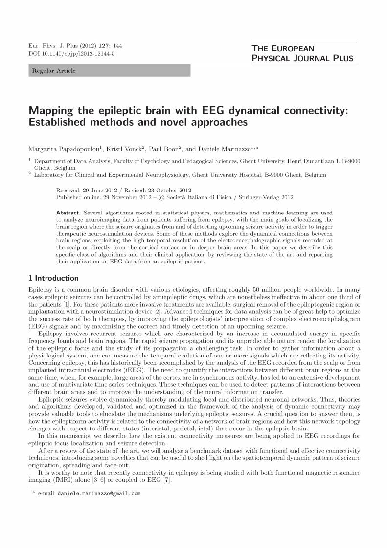
Fig. 2. Evolution of the maximum singular value σ over time (s). A: Coherence measured over the 27 scalp electrodes.An increase of σ is captured around the intracranial electroencephalographic onset indicating less diversity and more dominantcomponents. B: Coherence measured over the 60 cortical electrodes. A similar pattern with an earlier increase is observed inthe scalp electrodes.

innovation with respect to [47], we obtained this measure not only for the global matrix, but also for the single rowsand columns, representing for each channel the outgoing and incoming information, respectively. This allows to gatheradditional information on the spatiotemporal pattern of the seizure.

3.3 Results

We tracked the maximum singular value described above by observing its evolution over time. In order to evaluatethe performance of each one of the measures previously introduced, we computed both the total flow for all the nodesand the inflow and outflow for each one of them.

For the 27 scalp electrodes, coherence captured a drop in the maximum singular value before the time marked asintracranial electroencephalographic onset, followed by a sharp increase. The MSV remained high also after the endof the seizure (fig. 2, top). High values of the maximum singular value indicate less diversity but stronger componentswhich is in agreement with the concept that during the seizure the brain enters a more organized state. The inter-pretation of the momentary increase in independence of the nodes resulting in the initial drop in MSV, which couldbe possibly used for early seizure detection, will require further validation and discussion. For the 60 cortical contactsthere is a similar trend compared to the one in the scalp electrodes, with an increased maximum singular value duringthe electroencephalographic onset. However coherence in case of cortical electrodes proved a bit slower to detect theseizure onset compared to the scalp electrodes, and the MSV returned earlier to baseline values (see fig. 2, bottom,for an example).


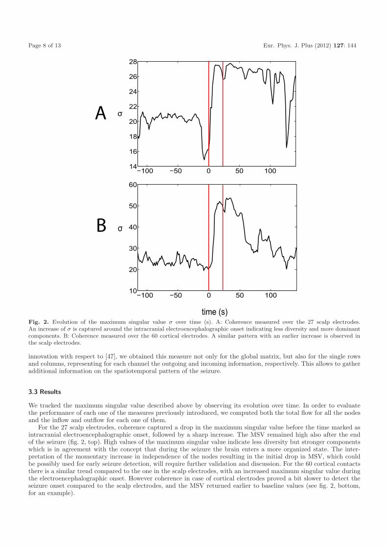
Fig. 3. Examples of the outgoing information captured by DTF in some cortical contacts for a single seizure (red lines indicateelectroencephalographic onset and termination). Some contacts present a clear drop of σ at the electroencephalographic onset,indicating that the components become more random during the seizure (top right), where others present this drop straightafter the electroencephalographic onset (top left). In other cases, the DTF captures a significant rise of σ straight after the endof the electroencephalographic onset (bottom).

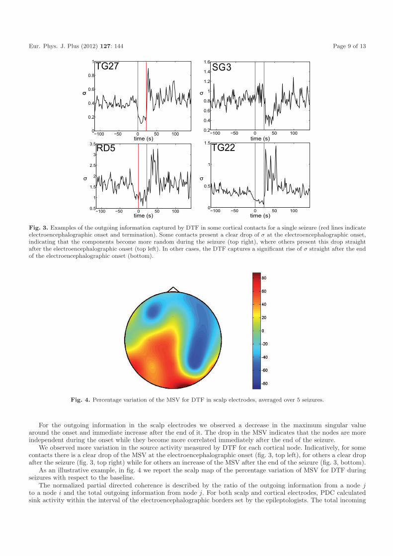
Fig. 4. Percentage variation of the MSV for DTF in scalp electrodes, averaged over 5 seizures.

For the outgoing information in the scalp electrodes we observed a decrease in the maximum singular valuearound the onset and immediate increase after the end of it. The drop in the MSV indicates that the nodes are moreindependent during the onset while they become more correlated immediately after the end of the seizure.

We observed more variation in the source activity measured by DTF for each cortical node. Indicatively, for somecontacts there is a clear drop of the MSV at the electroencephalographic onset (fig. 3, top left), for others a clear dropafter the seizure (fig. 3, top right) while for others an increase of the MSV after the end of the seizure (fig. 3, bottom).

As an illustrative example, in fig. 4 we report the scalp map of the percentage variation of MSV for DTF duringseizures with respect to the baseline.

The normalized partial directed coherence is described by the ratio of the outgoing information from a node jto a node i and the total outgoing information from node j. For both scalp and cortical electrodes, PDC calculatedsink activity within the interval of the electroencephalographic borders set by the epileptologists. The total incoming

of 13 Eur. Phys. J. Plus (2012) 127: 144

Fig. 5. Examples of outgoing information captured by PDC in some cortical contacts for a single seizure (red lines indicateelectroencephalographic onset and termination). Some contacts display an increase of σ at the electroencephalographic onsetindicating more dominant components (top left), where others present lower values during the seizure and a raise immediatelyafter it (top right). For some, high incoming activity is captured at the electroencephalographic onset (bottom).

Fig. 6. Percentage variation of the MSV for PDC in intracranial electrodes, at the onset of the seizure and 10 seconds afterthe onset, averaged over 5 seizures. The position of the electrodes reflects the scheme reported in fig. 1.

information quantified by PDC, shows variability among the 60 cortical contacts. The general trend in the 12 depthcontacts is in agreement with results of the total flow, as an increase in the MSV is observed for each one of them (fig. 5,top left). A decrease during the seizure and a raise after it is detected for some of the subdural contacts (fig. 5, top right)while a clear peak and then a drop after the end of the electrographic seizure is indicated in others (fig. 5, bottom).

In fig. 6 we report the map of the percentage variation of MSV for PDC at the onset of the seizure and 10 s afterwith respect to the baseline across the intracranial contacts. The maximum percentage variation is reported at oneextremity of the depth electrode (RD), confirming the presence of the seizure onset in the deep structures. After 10 s weobserved an increase also in the cortical electrodes, indicating spreading seizure activity. A similar pattern is observed


Fig. 7. Percentage variation of the MSV for PDC in intracranial electrodes, at the onset of the seizure and 10 seconds afterthe onset, averaged over 5 seizures. The position of the electrodes reflects the scheme reported in fig. 1.

for the outgoing connections as measured by the PDC (fig. 7), but in this case the pattern is more stable during theseizure. We can interpret this difference in view of a recent result [67] showing that in a hierarchical network theinformation going out from each node increases with the number of neighbors while the incoming information staysmore or less constant.

Moreover, and surprisingly, scalp electrodes are those for which the variation in the connectivity occurs the earliest.Previous studies [68] have reported that the predominance of global synchronization and overall volume conductioninduce a great variability of these scalp patterns, but this early modification of the dynamical connectivity could openinteresting perspectives for the development of therapeutic measures that may not require invasive recordings and givehints also on the location in space and time of the seizure termination.

4 Conclusions

We have provided an overview of the methods that explore dynamical connectivity in human EEG recordings tounderstand the physiological mechanisms underlying epilepsy, and also their application in the detection of the epilep-togenic region and prediction of seizure activity. We have shown that, for the analyzed case, some measures that havebeen previously employed for seizure detection can be also useful for focus localization. Furthermore the employedalgorithms are fast enough to allow for real-time application, thus making them amenable to clinical use. This paperpresents preliminary results and its purposes do not reach as far as evaluating their diagnostic value. The point wewish to make is that an integrated spatiotemporal approach, as well as a unified framework such as information theory,may represent an optimal strategy for the future of the analysis of epilepsy from a dynamical network perspective.

References

1. F. Mormann, R.G. Andrzejak, C.E. Elger, K. Lehnertz, Brain 130, 314 (2007).2. B.C. Jobst, T.M. Darcey, V.M. Thadani, D.W. Roberts, Epilepsia 51, 88 (2010).3. X. Zhang, F. Tokoglu, M. Negishi, J. Arora, S. Winstanley, D.D. Spencer, R.T. Constable, J. Neurosci. Methods 199, 129

(2011).4. M. Negishi, R. Martuzzi, E.J. Novotny, D.D. Spencer, R.T. Constable, Epilepsia 52, 1733 (2011).5. F. Pittau, C. Grova, F. Moeller, F. Dubeau, J. Gotman, Epilepsia 53, 1013 (2012).6. J. Zhang, W. Cheng, Z. Wang, Z. Zhang, W. Lu, G. Lu, J. Feng, PLoS ONE 7, e36733 (2012).7. T. Murta, A. Leal, M.I. Garrido, P. Figueiredo, NeuroImage 62, 1642 (2012).8. L.D. Iasemidis, J.C. Sackellares, H.P. Zaveri, W.J. Williams, Brain Topogr. 2, 187 (1990).

of 13 Eur. Phys. J. Plus (2012) 127: 144

9. J.P. Pijn, J. Van Neerven, A.Noest, F.H. Lopes da Silva, Electroencephalogr. Clin. Neurophysiol. 79, 371 (1991).10. F.H. Lopes da Silva, J.P. Pijn, W.J. Wadman, Prog. Brain Res. 102, 359 (1994).11. K. Lehnertz, C.E. Elger, Electroencephalogr. Clin. Neurophysiol. 95, 108 (1995).12. J. Martinerie, C. Adam, M. Le Van Quyen, M. Baulac, S. Clemenceau, B. Renault, F.J. Varela, Nature Med. 4, 1173 (1998).13. K.J. Friston, Brain Connectivity 1, 13 (2011).14. M.J. Kaminski, K.J. Blinowska, Biol. Cybern. 65, 203 (1991).15. C.W.J. Granger, Econometrica 37, 424 (1969).16. P.J. Franaszczuk, G.K. Bergey, Brain Topogr. 11, 13 (1998).17. B. Swiderski, S. Osowski, A. Cichocki, A. Rysz, Neurocomputing 72, 1575 (2009).18. C. Wilke, W. van Drongelen, M. Kohrman, B. He, Epilepsia 51, 564 (2010).19. P. van Mierlo, E. Carrette, H. Hallez, K. Vonck, D. Van Roost, P. Boon, S. Staelens, NeuroImage 56, 1122 (2011).20. A. Korzeniewska, C.M. Crainiceanu, R. Kus, P.J. Franaszczuk, N.E. Crone, Hum. Brain Mapp. 29, 1170 (2008).21. T. Mullen, Z.A. Acar, G. Worrell, S. Makeig, Modeling cortical source dynamics and interactions during seizure, in Proceed-

ings of the Annual International Conference of the IEEE Engineering in Medicine and Biology Society, Vol. 2011 (2011)pp. 1411–4.

22. A.J. Bell, T.J. Sejnowski, Neural Comput. 7, 1129 (1995).23. L.A. Baccala, K. Sameshima, Biol. Cybern. 84, 463 (2001).24. D.Y. Takahashi, L.A. Baccala, K.Sameshima, J. Appl. Stat. 34, 1259 (2007).25. G. Varotto, E. Visani, L. Canafoglia, S. Franceschetti, G. Avanzini, F. Panzica, Epilepsia 53, 359 (2012).26. P.J. Franaszczuk, G.K. Bergey, Biol. Cybern. 81, 3 (1999).27. A.J. Cadotte, T.B. DeMarse, T.H. Mareci, M.B. Parekh, S.S. Talathi, D.-U. Hwang, W.L. Ditto, M. Ding, P.R. Carney, J.

Neurosci. Methods 189, 121 (2010).28. G.R. Wu, F. Chen, D. Kang, X. Zhang, D. Marinazzo, H. Chen, IEEE Trans. Biomed. Eng. 58, 3088 (2011).29. H. Akaike, IEEE Trans. Autom. Control 19, 716 (1974).30. G. Schwarz, Ann. Stat.s 6, 461 (1978).31. B.G. Quinn, J. R. Stat. Soc. Ser. B 42, 182 (1980).32. R. Kohavi, A Study of Cross-Validation and Bootstrap for Accuracy Estimation and Model Selection, in IJCAI-95: Proceed-

ings of the 14th International Joint Conference on Artificial Intelligence, Vol. 2 (Morgan Kaufmann Publishers Inc., SanFrancisco, 1995) pp. 1137–1143.

33. S. Spencer, Epilepsia 43, 219 (2002).34. S.C. Ponten, F. Bartolomei, C.J. Stam, Clin. Neurophysiol. 118, 918 (2007).35. M.A. Kramer, E.D. Kolaczyk, H.E. Kirsch, Epilepsy Res. 79, 173 (2008).36. F. Wendling, P. Chauvel, A. Biraben, F. Bartolomei, Front. Syst. Neurosci. 4, 154 (2010).37. J.R. Terry, O. Benjamin, M.P. Richardson, Epilepsia 53, e166 (2012) doi: 10.1111/j.1528-1167.2012.03560.x.38. K. Lehnertz, C. Elger, Phys. Rev. Lett. 80, 5019 (1998).39. F. Mormann, K. Lehnertz, P. David, C.E. Elger, Physica D 144, 358 (2000).40. B. Litt, J. Echauz, Lancet Neurology 1, 22 (2002).41. F. Mormann, R.G. Andrzejak, T. Kreuz, C. Rieke, P. David, C.E. Elger, K. Lehnertz, Phys. Rev. E 67, 021912 (2003).42. M. Winterhalder, B. Schelter, T. Maiwald, A. Brandt, A. Schad, A. Schulze-Bonhage, J. Timmer, Clin. Neurophysiol. 117,

2399 (2006).43. I. Osorio, Y.-C. Lai, Chaos (N.Y.) 21, 033108 (2011).44. G. Ouyang, X. Li, Y. Li, X. Guan, Comput. Biol. Med. 37, 430 (2007).45. R.G. Andrzejak, D. Chicharro, C.E. Elger, F. Mormann, Clin. Neurophysiol. 120, 1465 (2009).46. M.S.D. Kerr, S.P. Burns, J. Gale, J. Gonzalez-Martinez, J. Bulacio, S.V. Sarma, Multivariate analysis of SEEG signals

during seizure, in Proceedings of the Annual International Conference of the IEEE Engineering in Medicine and Biology

Society, Vol. 2011 (2011) pp. 8279–8282.47. S. Santaniello, S.P. Burns, A.J. Golby, J.M. Singer, W.S. Anderson, S.V. Sarma, Epilepsy Behav. 22, S49 (2011).48. L.D. Iasemidis, D.-S. Shiau, J.C. Sackellares, P.M. Pardalos, A. Prasad, IEEE Trans. Biomed. Eng. 51, 493 (2004).49. M. Chavez, M. Le Van Quyen, V. Navarro, M. Baulac, J. Martinerie, IEEE Trans. Biomed. Eng. 50, 571 (2003).50. M. Palus, V. Komarek, Z. Hrncır, K. Sterbova, Phys. Rev. E 63, 046211 (2001).51. M. Eichler, Biol. Cybern. 94, 469 (2006).52. D.Y. Takahashi, L.A. Baccala, K. Sameshima, Biol. Cybern. 103, 463 (2010).53. L. Barnett, A.B. Barrett, A.K. Seth, Phys. Rev. Lett. 103, 238701 (2009).54. T. Schreiber, Phys. Rev. Lett. 85, 461 (2000).55. D. Marinazzo, M. Pellicoro, S. Stramaglia, Computational and Mathematical Methods in Medicine 2012, 303601 (2012).56. S. Sabesan, L.B. Good, K.S. Tsakalis, A. Spanias, D.M. Treiman, L.D. Iasemidis, IEEE transactions on neural systems and

rehabilitation engineering 17, 244 (2009).57. C. Stamoulis, B.S. Chang, Multiscale information for network characterization in epilepsy, in Proceedings of the Annual

International Conference of the IEEE Engineering in Medicine and Biology Society, Vol. 2011 (2011) pp. 5908–11.58. C. Stamoulis, L.J. Gruber, D.L. Schomer, B.S. Chang, Epilepsy Behav. 23, 471 (2012).59. M. Lindner, R. Vicente, V. Priesemann, M. Wibral, BMC Neurosci. 12, 119 (2011).60. J. Geweke, J. Am. Stat. Assoc. 77, 304 (1982).61. E. Florin, J. Gross, J. Pfeifer, G.R. Fink, L. Timmermann, NeuroImage 50, 577 (2010).


62. L. Barnett, A.K. Seth, J. Neurosci. Methods 201, 404 (2011).63. A. Korzeniewska, M. Manczak, M. Kaminski, K.J. Blinowska, S. Kasicki, J. Neurosci. Methods 125, 195 (2003).64. M. Kaminski, Phil. Trans. R. Soc. London. Ser. B Biol. Sci. 360, 947 (2005).65. L. Faes, G. Nollo, Assessing directional interactions among multiple physiological time series: the role of instantaneous

causality, in Proceedings of the Annual International Conference of the IEEE Engineering in Medicine and Biology Society,Vol. 2011 (2011) pp. 5919–5922.

66. K.J. Blinowska, Med. Biol. Eng. Comput. 49, 521 (2011).67. D. Marinazzo, G. Wu, M. Pellicoro, L. Angelini, S. Stramaglia, PLoS ONE 7, e45026 (2012).68. J.X. Tao, M. Baldwin, A. Ray, S. Hawes-Ebersole, J.S. Ebersole, Epilepsia 48, 2167 (2007).

epjplus - users.ugent.be

Documents